
Snowball Earth – Initiation and Hadley Cell Dynamics Aiko ... · Snowball Earth initiation would...
135
Aiko Voigt Berichte zur Erdsystemforschung Reports on Earth System Science 83 2010 Snowball Earth – Initiation and Hadley Cell Dynamics
Transcript of Snowball Earth – Initiation and Hadley Cell Dynamics Aiko ... · Snowball Earth initiation would...
Aiko Voigt
Berichte zur Erdsystemforschung
Reports on Earth System Science
832010
Snowball Earth – Initiation and Hadley Cell Dynamics

Aiko Voigt
Reports on Earth System Science
Berichte zur Erdsystemforschung 832010
832010
ISSN 1614-1199
Snowball Earth – Initiation and Hadley Cell Dynamics
Hamburg 2010
aus Berlin
ISSN 1614-1199
Als Dissertation angenommen vom Department Geowissenschaften der Universität Hamburg
auf Grund der Gutachten von Prof. Dr. Jochem MarotzkeundDr. Erich Roeckner
Hamburg, den 9. Juli 2010Prof. Dr. Jürgen OßenbrüggeLeiter des Departments für Geowissenschaften
Aiko VoigtMax-Planck-Institut für MeteorologieBundesstrasse 5320146 Hamburg Germany
Hamburg 2010
Snowball Earth – Initiation and Hadley Cell Dynamics
Aiko Voigt
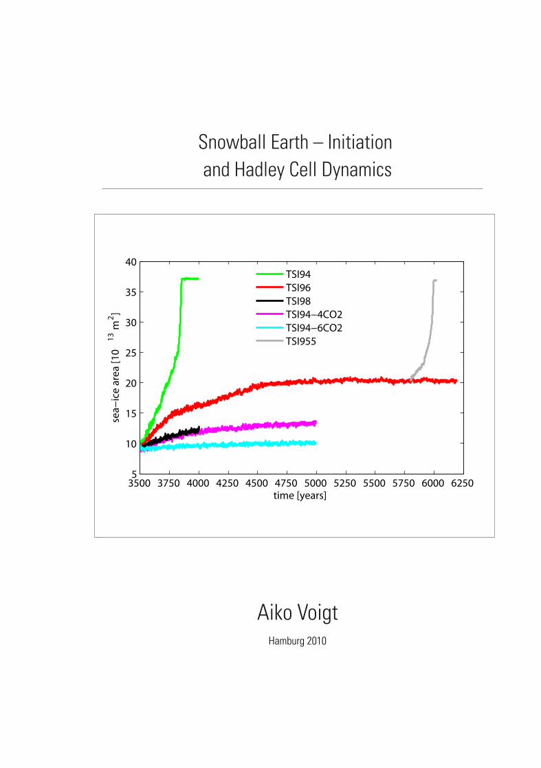
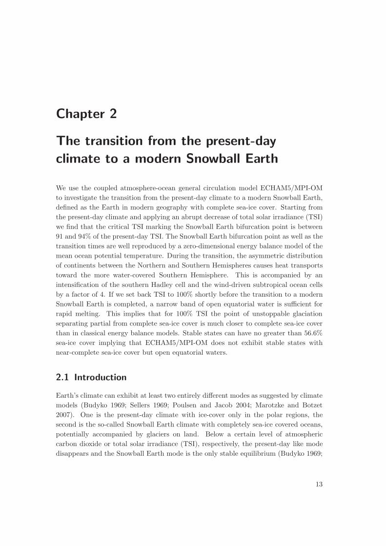
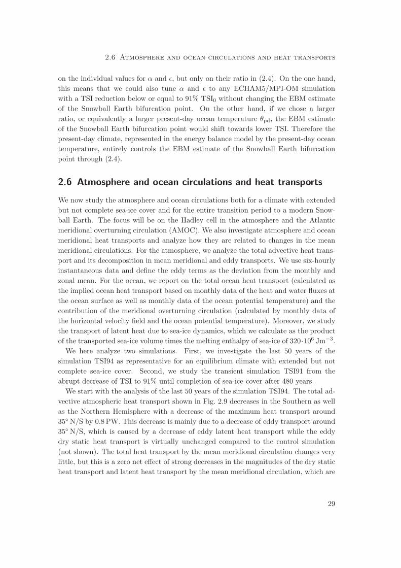
3500 3750 4000 4250 4500 4750 5000 5250 5500 5750 6000 62505
10
15
20
25
30
35
40
time [years]
sea−
ice
area
[10
13 m
2 ]
TSI94TSI96TSI98TSI94−4CO2TSI94−6CO2TSI955

Abstract
I use climate model simulations to investigate the initiation of a Snowball Earth for
present-day as well as Marinoan (∼ 635 million years before present) surface bound-
ary conditions, and to study the dynamics of the Hadley cell in a Snowball Earth
atmosphere.
Using the coupled atmosphere-ocean general circulation model ECHAM5/MPI-OM
in a present-day setup, I find that the modern Snowball Earth bifurcation point is
between 91 and 94% of the present-day total solar irradiance (TSI) when atmospheric
carbon dioxide is set to its pre-industrial level. The Snowball Earth bifurcation point as
well as the transition times are well reproduced by a zero-dimensional energy balance
model of the global-mean ocean potential temperature. During the transition, the
asymmetric distribution of continents between the Northern and Southern Hemispheres
causes heat transports toward the more water-covered Southern Hemisphere. Moreover,
stable states can have no greater than 56.6% sea-ice cover.
Using the same model in a Marinoan setup, I show that changing the surface bound-
ary conditions from present-day to Marinoan, which includes a shift of continents to low
latitudes, induces a global mean cooling of 4.6 K. The Marinoan Snowball Earth bifurca-
tion point for pre-industrial carbon dioxide is between 95.5 and 96% of the present-day
total TSI, illustrating that low-latitude continents facilitate Snowball Earth initiation.
A Snowball Earth for TSI reduced to 94% of its present-day value is prevented by
quadrupling atmospheric carbon dioxide with respect to its pre-industrial level. The
zero-dimensional energy balance model of global-mean ocean potential temperature
again successfully predicts the Snowball Earth bifurcation point. States with sea-ice
cover above 55% are unstable, akin to what I find for the present-day setup. This shows
that ECHAM5/MPI-OM does not exhibit stable states with near-complete sea-ice cover
but open equatorial waters. In summary, my results rebut previous conclusions that
Snowball Earth initiation would require ”extreme” forcings.
Using the atmosphere general circulation model ECHAM5, I investigate the tropical
meridional circulation of a Snowball Earth atmosphere. I find that the dynamics of the
Snowball Earth Hadley cell differ substantially from the dynamics of the present-day
Hadley cell. In the upper branch of the Snowball Earth Hadley cell, mean meridional
advection of mean absolute vorticity is not only balanced by eddy momentum flux diver-
gence but also by vertical diffusion. Vertical diffusion also contributes to the meridional
momentum balance as it decelerates the Hadley cell by downgradient momentum mix-
ing between its upper and lower branches. I conclude that neither axisymmetric Hadley
cell models based on angular momentum conservation nor eddy-permitting Hadley cell
models that neglect vertical diffusion of momentum are applicable to a Snowball Earth

atmosphere since both assume an inviscid upper Hadley cell branch. Because vertical
diffusion is important for the Hadley cell of a virtually dry Snowball Earth atmosphere,
dry atmospheres in general should not be considered as a-priori simpler testcases for
Hadley cell theories than moist atmospheres.
4
Contents
1 Introduction 7
1.1 Setting the scene . . . . . . . . . . . . . . . . . . . . . . . . . . . . . . . 7
1.2 Thesis objective . . . . . . . . . . . . . . . . . . . . . . . . . . . . . . . . 9
1.3 Thesis outline . . . . . . . . . . . . . . . . . . . . . . . . . . . . . . . . . 10
2 The transition from the present-day climate to a modern Snowball Earth 13
2.1 Introduction . . . . . . . . . . . . . . . . . . . . . . . . . . . . . . . . . . 13
2.2 Model . . . . . . . . . . . . . . . . . . . . . . . . . . . . . . . . . . . . . 15
2.3 Setup of ECHAM5/MPI-OM simulations . . . . . . . . . . . . . . . . . 17
2.4 Snowball Earth bifurcation point and transition time . . . . . . . . . . . 18
2.5 Comparison to a zero-dimensional energy balance model of mean ocean
potential temperature . . . . . . . . . . . . . . . . . . . . . . . . . . . . 26
2.6 Atmosphere and ocean circulations and heat transports . . . . . . . . . 29
2.7 Point of unstoppable glaciation . . . . . . . . . . . . . . . . . . . . . . . 35
2.8 Discussion . . . . . . . . . . . . . . . . . . . . . . . . . . . . . . . . . . . 40
2.9 Conclusions . . . . . . . . . . . . . . . . . . . . . . . . . . . . . . . . . . 46
3 Initiation of a Marinoan Snowball Earth in a state-of-the-art atmosphere-
ocean general circulation model 47
3.1 Introduction . . . . . . . . . . . . . . . . . . . . . . . . . . . . . . . . . . 47
3.2 Model and simulation setup . . . . . . . . . . . . . . . . . . . . . . . . . 49
3.2.1 Model setup . . . . . . . . . . . . . . . . . . . . . . . . . . . . . . 49
3.2.2 Simulation setup . . . . . . . . . . . . . . . . . . . . . . . . . . . 55
3.3 Marinoan control climate and comparison to the pre-industrial control
climate . . . . . . . . . . . . . . . . . . . . . . . . . . . . . . . . . . . . . 57
3.3.1 Surface climate . . . . . . . . . . . . . . . . . . . . . . . . . . . . 57
3.3.2 Meridional circulations and heat transports of atmosphere and
ocean . . . . . . . . . . . . . . . . . . . . . . . . . . . . . . . . . 58
3.3.3 One-dimensional energy balance model . . . . . . . . . . . . . . . 65
3.4 Snowball Earth bifurcation point and maximum stable sea-ice cover . . 74
3.5 Prediction of the Snowball Earth bifurcation point and transition times
by a zero-dimensional energy balance model . . . . . . . . . . . . . . . . 77
3.6 Energy fluxes at the top of atmosphere and at the surface . . . . . . . . 81
5
Contents
3.7 Discussion . . . . . . . . . . . . . . . . . . . . . . . . . . . . . . . . . . . 83
3.8 Conclusion . . . . . . . . . . . . . . . . . . . . . . . . . . . . . . . . . . 85
3.A Sensitivity to vertical mixing parameters of the ocean model . . . . . . . 86
4 Equinox Hadley cell dynamics in a Snowball Earth atmosphere 89
4.1 Introduction . . . . . . . . . . . . . . . . . . . . . . . . . . . . . . . . . . 90
4.2 Model and simulation setup . . . . . . . . . . . . . . . . . . . . . . . . . 91
4.3 Meridional structure of the Snowball Earth atmosphere . . . . . . . . . 93
4.4 Dynamics of the Snowball Earth Hadley cell . . . . . . . . . . . . . . . . 97
4.4.1 Zonal momentum balance . . . . . . . . . . . . . . . . . . . . . . 97
4.4.2 Meridional momentum budget . . . . . . . . . . . . . . . . . . . 98
4.5 Influence of vertical momentum diffusion on Hadley cell strength . . . . 100
4.5.1 Hypothetical Hadley cell strength in an inviscid atmosphere . . . 100
4.5.2 Simulations with suppressed vertical diffusion of horizontal mo-
mentum . . . . . . . . . . . . . . . . . . . . . . . . . . . . . . . . 103
4.6 Influence of the diurnal cycle and the parameterization of eddy viscosity 106
4.7 Discussion . . . . . . . . . . . . . . . . . . . . . . . . . . . . . . . . . . . 109
4.8 Conclusions . . . . . . . . . . . . . . . . . . . . . . . . . . . . . . . . . . 112
5 Conclusions and Outlook 113
5.1 Conclusions . . . . . . . . . . . . . . . . . . . . . . . . . . . . . . . . . . 113
5.2 Outlook . . . . . . . . . . . . . . . . . . . . . . . . . . . . . . . . . . . . 115
Bibliography 117
Acknowledgements 127
6
Chapter 1
Introduction
1.1 Setting the scene
Today’s Earth comes as a comfortable place in the universe with moderate temperatures
and liquid water at the surface, the latter being vital to the existence of life on Earth
as we know it. Despite repeated excursions to warmer and colder climates, these
conditions have prevailed for longer than the last 500 million years. Nevertheless, if
we look only a bit further back in Earth’s history, to the Neoproterozoic (1000 - 542
million years before present, Ma), we encounter evidence that Earth might have spent
millions of years in a fundamentally different climate state (Kirschvink 1992; Hoffman
et al. 1998; Hoffman and Schrag 2002). In this state, surface temperatures would be far
below freezing even at the equator, implying that hardly any liquid surface water would
be present, and oceans would be completely covered by sea ice. Earth would appear
as a white planet from space, which is why this state is commonly dubbed ”Snowball
Earth.”
To arrive at the Snowball Earth hypothesis requires one to combine geology and
climate physics. On the one hand, glacial deposits strongly support the existence of
wide-spread sea-level land glaciers in the tropics during two Neoproterozoic periods,
the Sturtian (∼ 710 Ma) and the Marinoan (∼ 635 Ma) (Evans 2000; Trindade and
Macouin 2007; Macdonald et al. 2010). On the other hand, simple enery balance models
(Budyko 1969; Sellers 1969) suggest that once ice passes 30 degrees latitude, a runaway
ice-albedo feedback leads to global ice cover. Kirschvink (1992) combined both pieces
and came up with the idea that low-latitude glaciers by virtue of the runaway ice-albedo
feedback require the entire Earth to be in deep freeze, the Snowball Earth.
In its complete form, the Snowball Earth hypothesis encompasses Snowball Earth
initiation triggered by a drawdown of atmospheric greenhouse gases, residence in deep
freeze for millions of years with slow but continous build-up of atmospheric carbon
dioxide, and rapid deglaciation by massive carbon dioxide levels followed by a super-
greenhouse. While the geological community continues a passionate debate whether the
sedimentary record is compatible with the Snowball Earth hypothesis, the latter has
also stimulated climate modellers to investigate its compatibility with climate physics.
7
Chapter 1 Introduction
This task clearly calls for models that are far more complex and comprehensive than
the energy balance models that Kirshvink relied on. It is commonly accepted that Earth
exhibits both the present-day like climate with only little sea-ice cover and the Snowball
Earth climate with global sea-ice cover for present-day total solar irradiance (Marotzke
and Botzet 2007). The role of climate modelling is hence to investigate if Snowball Earth
initiation as well as Snowball Earth deglaciation are possible for values of total solar
irradiance and/or atmospheric carbon dioxide that one thinks have prevailed during
the Sturtian and Marinoan Snowball periods. Deglaciation long seemed to be the more
difficult problem of the two (Pierrehumbert 2005), but recent studies have shown that
dust makes deglaciation possible at carbon dioxide levels compatible with proxy data
(Abbot and Pierrehumbert 2010; Abbot and Halevy 2010; Le Hir et al. 2010). In the
case of initiation, recent years have seen an increasing number of climate modelling
studies concluding that completely frozen oceans require ”extreme” forcings (Chandler
and Sohl 2000; Poulsen et al. 2001; Poulsen 2003; Poulsen and Jacob 2004) that might
be considered unrealistic for the Neoproterozoic. At the same time, Hyde et al. (2000)
and Peltier et al. (2004) found so-called ”Slushball Earth” solutions that permit tropical
land glaciers and open equatorial water simultaneously. Despite severe limitations of
this model, including the disregard of atmosphere and ocean dynamics, these solutions
have been supported in an atmospheric general circulation model coupled to a slab
ocean and prescribed full continental glaciation (Hyde et al. 2000; Baum and Crowley
2001). Moreover, Chandler and Sohl (2000) and Micheels and Montenari (2008) found,
also using atmosphere general circulation models coupled to slab oceans, solutions with
equatorial land masses below freezing in conjunction with almost but not completely
frozen oceans. As a result, the apparent difficulties in freezing the entire ocean combined
with the possibility that equatorial land glaciers might not require completely frozen
oceans evoked the impression that the Snowball Earth hypothesis seems implausible
from the perspective of climate modelling. As a consequence, attention shifted to the
Slushball Earth hypothesis (Lubick 2002; Kaufman 2007; Kerr 2010). In this thesis, I
revisit Snowball Earth initiation with the hitherto best climate model applied to this
problem. This model includes all physics found to be essential for Snowball Earth
initiation, namely ocean dynamics, sea-ice dynamics, and interactive clouds.
Apart from using climate models to test the plausibility of the Snowball Earth hy-
pothesis, the Snowball Earth offers a potentially fruitful testbed for atmospheric dy-
namicists. Its atmosphere is characterized by cold temperatures, and as a consequence
water is largely eliminated from the atmosphere. The influence of moisture on the
large-scale circulation, an issue that without doubt ranks among the most challenging
topics in atmospheric science today, is hence virtually removed. This turns the Snowball
Earth into an example of a dry atmosphere As the challenge of atmospheric dynamics
is not in ascertaining the underlying dynamical equations, which are essentially known,
but in distilling the primal processes and in neglecting the others, a dry atmosphere is
8
1.2 Thesis objective
commonly thought of as a convenient starting point if one seeks to develop theories for
atmospheric dynamics.
One of the most prominent examples for this approach is the Hadley circulation, a
synonym for the tropical overturning circulation in the troposphere (see Lorenz (1967)
for a historic review, and Schneider (2006) for a summary of recent progress). Pio-
neered by Schneider (1977) and Held and Hou (1980), important understanding has
been gained by considering axisymmetric atmospheres. Thanks to increasing access to
computing resources and progress in atmospheric modelling, however, one now seems in
good position to study Hadley cell dynamics including the effect of non-axisymmetric
motions, i.e. eddies, over a wide range of external parameters that one believes ulti-
mately should control Hadley cell strength and extent. Recent years have seen consid-
erable progress in this direction (Walker and Schneider 2005, 2006), largely by using the
idealized general circulation model introduced in Schneider and Walker (2006). This
model does resolve the large-scale circulation but only crudely accounts for subgrid
physical processes. It is therefore essential to verify these results in a general circula-
tion model with comprehensive physics but, surprisingly, this has not been done yet.
By studying the Hadley cell in a Snowball Earth atmosphere with a state-of-the-art
general circulation model, we hope to take a first step towards closing this gap.
1.2 Thesis objective
My thesis aims at answering the following research questions brought up in the previous
section.
1. Initiation of a Snowball Earth
I apply the atmosphere-ocean general circulation model ECHAM5/MPI-OM to tackle
the following issues:� How much reduction of radiative forcing, in particular how much reduction of
total solar irradiance, is needed to trigger Snowball Earth initiation? How much
increase of atmospheric carbon dioxide is needed to prevent a Snowball Earth?� How does the climate system behave during the transition to a Snowball Earth?
In particular, how do atmosphere and ocean heat transports change?� How close can sea ice invade the tropics before global sea-ice cover is triggered?� Is the location of continents important for Snowball Earth initiation?� Can we use simpler models to understand certain aspects of Snowball Earth
initiation?
9
Chapter 1 Introduction
2. Atmospheric dynamics of a Snowball Earth
Using the atmosphere general circulation model ECHAM5, I focus on:� What characterizes the Hadley cell of a Snowball Earth atmosphere?� How does this compare to dry Hadley cell theories?
1.3 Thesis outline
My thesis contains three chapters written in the style of journal publications. One
chapter has already been published while the other two are currently being prepared for
submission. As a consequence, they contain their own introduction, model description,
and conclusions, and can be read largely on their own. Two chapters are devoted to
Snowball Earth initiation for present-day (Chapter 2) and Marinoan surface boundary
conditions (Chapter 3), one chapter to the Snowball Earth Hadley cell (Chapter 4).� Chapter 2 investigates the sensitivity of the present-day climate to abrupt re-
ductions of total solar irradiance. I estimate the transition time to a modern
Snowball Earth and the Snowball Earth bifurcation point. Both are compared to
a zero-dimensional energy balance of global-mean ocean potential temperature. I
moreover analyze atmosphere and ocean heat transports during the entire transi-
tion from the present-day climate to a Snowball Earth and study how close sea ice
can invade the tropics before the climate system becomes unstable. This chapter
has been published in Climate Dynamics1, and is reproduced here with editorial
adjustments.� In Chapter 3, I study if the location of continents influences what I found
in Chapter 2. To this end, I change the surface boundary conditions to be
representative of the Marinoan period, which includes a shift of continents to
low latitudes, and generate a Marinoan control climate for present-day total solar
irradiance and pre-industrial greenhouse gas concentrations using the same model
as in Chapter 2. The climatic consequences of the change in surface boundary
conditions are quantified by means of a one-dimensional energy balance model of
zonal mean surface temperature. I reinvestigate the Snowball Earth bifurcation
point and maximum stable sea-ice cover for the Marinoan setup. This allows
me to contribute to the debate if a Snowball Earth hypothesis is compliant with
the current knowledge of climate modelling. This chapter is in preparation for
submission to Journal of Geophysical Research2.
1Voigt, A. and J. Marotzke, 2009: The transition from the present-day climate to a modern Snowball
Earth. Clim. Dyn., doi:0.1007/s00382-009-0633-5.2Voigt, A., D. S. Abbot, R. T. Pierrehumbert, and J. Marotzke, 2010: Initiation of a Marinoan
10
1.3 Thesis outline� Chapter 4 deals with the dynamics of a Snowball Earth Hadley cell. I analyze
the zonal and meridional momentum balances and investigate the role of vertical
momentum diffusion for the Hadley cell using thought experiments and simula-
tions. I compare my results to Hadley cell theories and discuss the implications
of my simulations on the latter. This chapter is in preparation for submission to
Journal of Atmospheric Sciences3.
The thesis closes with a summary of my main findings in Chapter 5, in which I also
propose directions of future research.
Snowball Earth in a state-of-the-art atmosphere-ocean general circulation model, J. Geophys. Res.,
in preparation.3Voigt, A., I. M. Held, and J. Marotzke, 2010: Equinox Hadley cell dynamics in a Snowball Earth
atmosphere, J. Atmos. Sci., in preparation.
11

Chapter 2
The transition from the present-day
climate to a modern Snowball Earth
We use the coupled atmosphere-ocean general circulation model ECHAM5/MPI-OM
to investigate the transition from the present-day climate to a modern Snowball Earth,
defined as the Earth in modern geography with complete sea-ice cover. Starting from
the present-day climate and applying an abrupt decrease of total solar irradiance (TSI)
we find that the critical TSI marking the Snowball Earth bifurcation point is between
91 and 94% of the present-day TSI. The Snowball Earth bifurcation point as well as the
transition times are well reproduced by a zero-dimensional energy balance model of the
mean ocean potential temperature. During the transition, the asymmetric distribution
of continents between the Northern and Southern Hemispheres causes heat transports
toward the more water-covered Southern Hemisphere. This is accompanied by an
intensification of the southern Hadley cell and the wind-driven subtropical ocean cells
by a factor of 4. If we set back TSI to 100% shortly before the transition to a modern
Snowball Earth is completed, a narrow band of open equatorial water is sufficient for
rapid melting. This implies that for 100% TSI the point of unstoppable glaciation
separating partial from complete sea-ice cover is much closer to complete sea-ice cover
than in classical energy balance models. Stable states can have no greater than 56.6%
sea-ice cover implying that ECHAM5/MPI-OM does not exhibit stable states with
near-complete sea-ice cover but open equatorial waters.
2.1 Introduction
Earth’s climate can exhibit at least two entirely different modes as suggested by climate
models (Budyko 1969; Sellers 1969; Poulsen and Jacob 2004; Marotzke and Botzet
2007). One is the present-day climate with ice-cover only in the polar regions, the
second is the so-called Snowball Earth climate with completely sea-ice covered oceans,
potentially accompanied by glaciers on land. Below a certain level of atmospheric
carbon dioxide or total solar irradiance (TSI), respectively, the present-day like mode
disappears and the Snowball Earth mode is the only stable equilibrium (Budyko 1969;
13
Chapter 2 The transition to a modern Snowball Earth
Sellers 1969). We will refer to this critical threshold as the Snowball Earth bifurcation
point. Here, we use the state-of-the-art climate model ECHAM5/MPI-OM to study
the transition from the present-day climate to a hypothetical modern Snowball Earth,
which we define as the Earth in modern geography with complete sea-ice cover.
The Snowball Earth is of interest both from a geological as well as a climate modelling
perspective. On the one hand, based on glacial deposits in Neoproterozoic (∼ 750-550
Ma) rock sequences it has been argued that several Snowball Earth events might have
occurred during Earth’s history (Kirschvink 1992; Hoffman et al. 1998). On the other
hand, the Snowball Earth challenges climate modellers to confront their models and
understanding of the climate system with the extreme climate of a Snowball Earth. In-
deed, the work of Budyko (1969) and Sellers (1969), who used one-dimensional energy
balance models and a temperature-dependent albedo parametrization to show that the
entire Earth might become ice-covered if TSI was decreased by a few percent, stimu-
lated a whole series of Snowball Earth modelling studies using the whole hierarchy of
climate models, ranging from energy balance models (e.g., Held and Suarez 1974; North
1975), over Earth system models of intermediate complexity (e.g., Stone and Yao 2004;
Donnadieu et al. 2004b; Romanova et al. 2006; Lewis et al. 2007), and atmosphere
general circulation models with simplified ocean models (e.g., Jenkins and Frakes 1998;
Chandler and Sohl 2000), to fully coupled atmosphere-ocean general circulation models
(e.g., Poulsen et al. 2001; Poulsen and Jacob 2004). Some studies even incorporated
dynamic ice sheet models (Hyde et al. 2000; Crowley et al. 2001; Peltier et al. 2004).
Most studies attempted to estimate the Snowball Earth bifurcation point of the ap-
plied climate model by simulating the equilibrium climates for reduced values of TSI
(justified by the “faint young sun” phenomenon) and/or reduced levels of atmospheric
carbon dioxide. Several studies addressed the importance of various elements of the
climate system such as ocean dynamics (Poulsen et al. 2001), surface winds (Poulsen
and Jacob 2004), sea-ice dynamics (Lewis et al. 2007), sea-ice glaciers (Goodman and
Pierrehumbert 2003; Pollard and Kasting 2005), and clouds (Le Hir et al. 2007; Poulsen
and Jacob 2004), including their representation in the models.
However, except for the work of Donnadieu et al. (2004b), who used an Earth sys-
tem model of intermediate complexity, previous studies focussed on whether a distinct
combination of reduction in TSI and atmospheric carbon dioxide triggered a Snowball
Earth, and they did not attempt to model the entire transition between the present-
day like mode and the Snowball Earth mode. Instead of initializing the models from
the present-day like mode, initial ocean temperatures were chosen to reduce the time
required to reach equilibrium (e.g., Poulsen and Jacob 2004). In contrast, we here start
our simulations from the pre-industrial control climate of our climate model and apply
an abrupt decrease of total solar irradiance or atmospheric CO2 to trigger the transi-
tion to a modern Snowball Earth. We thereby follow the same experimental strategy
as Marotzke and Botzet (2007), but we apply a wide range of TSI reductions instead
14
2.2 Model
of a single reduction of TSI to 0.01% of its today’s value. In this study, we assess the
following three issues.
First, we estimate both the Snowball Earth bifurcation point of the climate model
ECHAM5/MPI-OM and the time needed to complete the transition from the present-
day climate to a Snowball Earth. To our knowledge, there is only one study, with a
simple energy balance model climate model, that estimates the transition time after a
time-dependent reduction of TSI by 30% (Walsh and Sellers 1993).
Second, we analyze the response of the atmosphere and ocean heat transports and
mean meridional circulations during the transition, with a focus on the Hadley cell and
the Atlantic meridional overturning circulation. We compare our findings to the study
of Donnadieu et al. (2004b) and find important differences.
Third, we study the degree of sea-ice cover that guarantees an unstoppable glaciation.
This allows us to assess which extent of open equatorial water is possible, that is,
whether our climate model exhibits solutions with near-complete sea-ice cover but open
equatorial waters.
The paper is organized as follows. Section 2 describes the climate model, and Sect. 3
the setup of the ECHAM5/MPI-OM simulations. Section 4 investigates the Snowball
Earth bifurcation point. Section 5 presents a zero-dimensional energy balance model of
the mean ocean potential temperature and compares the results of the climate model
ECHAM5/MPI-OM with this zero-dimensional model. Section 6 analyzes the atmo-
sphere and ocean meridional circulations and heat transports, followed in Sect. 7 by
an investigation of the degree of sea-ice cover needed for an unstoppable glaciation.
Section 8 gives a general discussion of the results, Sect. 9 follows with conclusions.
2.2 Model
We use the the Max Planck Institute for Meteorology coupled atmosphere-ocean general
circulation model ECHAM5.3.02p2/MPI-OM-1.2.3p2 (labelled by ECHAM5/MPI-OM
in the following). The atmosphere component ECHAM5 is the fifth generation of the
ECHAM model series that originally evolved from the weather prediction model of the
European Centre for Medium Range Weather Forecasts. The details of ECHAM5 are
comprehensively described in Roeckner et al. (2003). ECHAM5 employs a dynamical
spectral core with vorticity, divergence, temperature, and the logarithm of surface
pressure being represented in the horizontal by a truncated series of spherical harmonics.
In the vertical a hybrid sigma-pressure coordinate system is applied. The shortwave
radiation scheme (Fouquart and Bonnel 1980) uses 4 spectral bands. For longwave
radiation ECHAM5 employs the Rapid Radiative Transfer Model (RRTM) developed
by Mlawer et al. (1997) with 16 spectral bands. ECHAM5 uses a stratiform cloud
scheme including a cloud microphysical scheme and prognostic equations for the vapour,
liquid, and ice phase, respectively. Snow at the surface and the inception of snow at
15
Chapter 2 The transition to a modern Snowball Earth
the canopy are modeled explicitly. Most important for our study is the treatment of
surface albedo. The grid-mean surface albedo depends on a prescribed background
albedo. Snow on land changes this background albedo according to the fractional
snow cover of the grid cell. The fractional snow cover itself is a function of the snow
depth measured in metres of water equivalent, but also of the orographic standard
deviation so that sloping terrains require a larger snow depth than flat terrains to
reach the same fractional snow cover. The albedo of snow on land depends on the land
surface temperature and ranges from 0.3 at 0◦ C to 0.8 at or below −5◦ C. Moreover,
the shielding effect of forests is accounted for in the surface albedo. In forest areas
the surface albedo is further modified by snow cover on the canopy and the resulting
canopy albedo.
The ocean component MPI-OM employs the primitive equations on an orthogonal
curvilinear C-grid (Arakawa and Lamb 1977), with the North Pole shifted to Greenland
to avoid a singularity at the geographical North Pole. The grid South Pole is located
over Antarctica. In the vertical, the model employs unevenly spaced z-levels with
the bottom topography being resolved by way of partial grid cells (Wolff et al. 1997).
Technical details of MPI-OM can be found in Marsland et al. (2003). We here only
give a short description of the embedded sea-ice model, which follows the dynamics
of Hibler (Hibler 1979) while the thermodynamics are incorporated by a zero-layer
Semtner model relating changes in sea-ice thickness to a balance of radiant, turbulent,
and oceanic heat fluxes (Semtner 1976). The freezing point of sea water is fixed to
−1.9◦ C independent of salinity. Snow on ice is explicitly modeled, including snow/ice
transformation when the snow/ice interface sinks below the sea level because of snow
loading. The effect of ice formation and melting is accounted for by assuming a sea-ice
salinity of 5. The albedo of bare sea ice depends on the ice surface temperature and
ranges from 0.55 at 0◦ C to 0.75 at or below −1◦ C. Snow on sea ice leads to a significant
albedo increase: if the water equivalent of snow depth is larger than 0.01 m, the sea ice
is treated as being snow-covered. The albedo of snow-covered sea ice depends on the
snow surface temperature and ranges from 0.65 at 0◦ C to 0.8 at or below −1◦ C. Sea
ice thickness is limited to about 8 m, 75% of the thickness of the top layer of MPI-OM,
to avoid the problem of dry model levels.
The atmosphere model ECHAM5 is coupled to the ocean model MPI-OM via the
OASIS3 coupler (Valcke et al. 2003) with a coupling time step of one day. The ocean
passes the sea surface temperature, sea-ice concentration and thickness, snow depth
on ice, and ocean surface velocities to the atmosphere. The atmosphere provides the
wind stress, heat flux, freshwater flux including river runoff and glacier calving, and
10 m wind speed to the ocean model. In the presence of sea ice the fluxes are calculated
separately for sea-ice covered and open water parts of the grid cells. No flux adjustments
are applied.
ECHAM5/MPI-OM has been extensively and successfully evaluated against obser-
16
2.3 Setup of ECHAM5/MPI-OM simulations
vations (Hagemann et al. 2004; Jungclaus et al. 2006; Roeckner et al. 2006; Wild
and Roeckner 2006) and was used for the integrations for the fourth assessment re-
port of the Intergovernmental Panel on Climate Change (Brasseur and Roeckner 2005;
Bengtsson et al. 2006; Landerer et al. 2007). Here, we use the low-resolution version
of ECHAM5/MPI-OM to perform long simulations of up to 1000 years length. The
atmosphere component uses 19 vertical levels and has a horizontal resolution of T31
(∼ 3.75 degrees). The ocean model uses 40 vertical levels and has a horizontal resolution
varying between 30 km near Greenland and 390 km in the tropical Pacific.
In contrast to most Snowball Earth model simulations, the location of continents,
the mountain topography and the ocean bathymetry are all kept at their present-
day values. Orbital parameters have modern values. Ozone follows the 1980-1991
climatology of Fortuin and Kelder (1998). Vegetation is prescribed according to a
present-day climatology with monthly varying vegetation cover and leaf area indices
for each surface grid cell. Land glaciers are fixed to their present-day extent. While
the choice of modern boundary conditions inhibits the simulation of a Neoproterozoic
Snowball Earth, it enables us to start our simulations from the present-day control
climate and hence to simulate the entire transition from the present-day climate to a
modern Snowball Earth. Atmospheric greenhouse gases are kept at pre-industrial levels
(CO2 = 286.2 ppm, CH4=805.6 ppb, N2O=276.7 ppb, no cfc), except for one simulation
where we set the atmospheric CO2 concentration to 0.1% of its pre-industrial value,
i.e., 0.2862 ppm. This will then be stated explicitly.
2.3 Setup of ECHAM5/MPI-OM simulations
We conduct two different sets of ECHAM5/MPI-OM simulations. In the first set,
we estimate the Snowball Earth bifurcation point by starting from the present-day
control climate of ECHAM5/MPI-OM (simulation CTRL with today’s TSI, TSI0 =
1367 Wm−2, and pre-industrial greenhouse gas levels) but decreasing TSI with respect
to TSI0. The model is run until it reaches a new equilibrium, which is either a modern
Snowball Earth characterized by complete sea-ice cover or a climate with extended but
not complete sea-ice cover. As a byproduct we also obtain the transition times to a
modern Snowball Earth as a function of the reductions in TSI as well as the atmospheric
and oceanic dynamics and heat transports during the entire transition. We also conduct
one experiment where we keep TSI at its present-day value but reduce atmospheric CO2
to 0.1% of its pre-industrial value (simulation noCO2). All simulations of this first set
are summarised in Table 2.1.
In the second set of simulations, we investigate which degree of sea-ice cover guar-
antees an unstoppable glaciation. When the climate model is on the way to a modern
Snowball Earth due to a decrease of TSI below the Snowball Earth bifurcation point,
we increase TSI abruptly at different stages of sea-ice cover before the transition to a
17
Chapter 2 The transition to a modern Snowball Earth
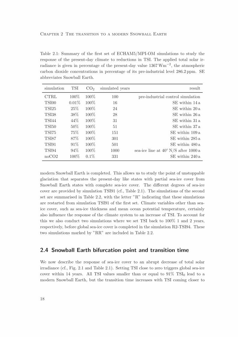
Table 2.1: Summary of the first set of ECHAM5/MPI-OM simulations to study the
response of the present-day climate to reductions in TSI. The applied total solar ir-
radiance is given in percentage of the present-day value 1367 Wm−2, the atmospheric
carbon dioxide concentrations in percentage of its pre-industrial level 286.2 ppm. SE
abbreviates Snowball Earth.
simulation TSI CO2 simulated years result
CTRL 100% 100% 100 pre-industrial control simulation
TSI00 0.01% 100% 16 SE within 14 a
TSI25 25% 100% 24 SE within 20 a
TSI38 38% 100% 28 SE within 26 a
TSI44 44% 100% 31 SE within 31 a
TSI50 50% 100% 51 SE within 37 a
TSI75 75% 100% 151 SE within 109 a
TSI87 87% 100% 301 SE within 285 a
TSI91 91% 100% 501 SE within 480 a
TSI94 94% 100% 1000 sea-ice line at 40◦ N/S after 1000 a
noCO2 100% 0.1% 331 SE within 240 a
modern Snowball Earth is completed. This allows us to study the point of unstoppable
glaciation that separates the present-day like states with partial sea-ice cover from
Snowball Earth states with complete sea-ice cover. The different degrees of sea-ice
cover are provided by simulation TSI91 (cf., Table 2.1). The simulations of the second
set are summarised in Table 2.2, with the letter ”R” indicating that these simulations
are restarted from simulation TSI91 of the first set. Climate variables other than sea-
ice cover, such as sea-ice thickness and mean ocean potential temperature, certainly
also influence the response of the climate system to an increase of TSI. To account for
this we also conduct two simulations where we set TSI back to 100% 1 and 2 years,
respectively, before global sea-ice cover is completed in the simulation R2-TSI94. These
two simulations marked by ”RR” are included in Table 2.2.
2.4 Snowball Earth bifurcation point and transition time
We now describe the response of sea-ice cover to an abrupt decrease of total solar
irradiance (cf., Fig. 2.1 and Table 2.1). Setting TSI close to zero triggers global sea-ice
cover within 14 years. All TSI values smaller than or equal to 91% TSI0 lead to a
modern Snowball Earth, but the transition time increases with TSI coming closer to
18
2.4 Snowball Earth bifurcation point and transition time
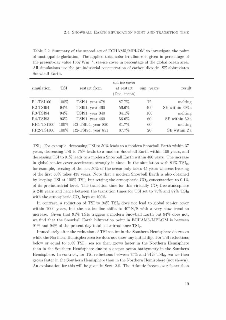
Table 2.2: Summary of the second set of ECHAM5/MPI-OM to investigate the point
of unstoppable glaciation. The applied total solar irradiance is given in percentage of
the present-day value 1367 Wm−2, sea-ice cover in percentage of the global ocean area.
All simulations use the pre-industrial concentration of carbon dioxide. SE abbreviates
Snowball Earth.
sea-ice cover
simulation TSI restart from at restart sim. years result
(Dec. mean)
R1-TSI100 100% TSI91, year 478 87.7% 72 melting
R2-TSI94 94% TSI91, year 460 56.6% 400 SE within 393 a
R3-TSI94 94% TSI91, year 340 34.1% 100 melting
R4-TSI93 93% TSI91, year 460 56.6% 60 SE within 52 a
RR1-TSI100 100% R2-TSI94, year 850 81.7% 60 melting
RR2-TSI100 100% R2-TSI94, year 851 87.7% 20 SE within 2 a
TSI0. For example, decreasing TSI to 50% leads to a modern Snowball Earth within 37
years, decreasing TSI to 75% leads to a modern Snowball Earth within 109 years, and
decreasing TSI to 91% leads to a modern Snowball Earth within 480 years. The increase
in global sea-ice cover accelerates strongly in time. In the simulation with 91% TSI0,
for example, freezing of the last 50% of the ocean only takes 45 years whereas freezing
of the first 50% takes 435 years. Note that a modern Snowball Earth is also obtained
by keeping TSI at 100% TSI0 but setting the atmospheric CO2 concentration to 0.1%
of its pre-industrial level. The transition time for this virtually CO2-free atmosphere
is 240 years and hence between the transition times for TSI set to 75% and 87% TSI0with the atmospheric CO2 kept at 100%.
In contrast, a reduction of TSI to 94% TSI0 does not lead to global sea-ice cover
within 1000 years, but the sea-ice line shifts to 40◦ N/S with a very slow trend to
increase. Given that 91% TSI0 triggers a modern Snowball Earth but 94% does not,
we find that the Snowball Earth bifurcation point in ECHAM5/MPI-OM is between
91% and 94% of the present-day total solar irradiance TSI0.
Immediately after the reduction of TSI sea ice in the Southern Hemisphere decreases
while the Northern Hemisphere sea ice does not show any initial dip. For TSI reductions
below or equal to 50% TSI0, sea ice then grows faster in the Northern Hemisphere
than in the Southern Hemisphere due to a deeper ocean bathymetry in the Southern
Hemisphere. In contrast, for TSI reductions between 75% and 91% TSI0, sea ice then
grows faster in the Southern Hemisphere than in the Northern Hemisphere (not shown).
An explanation for this will be given in Sect. 2.8. The Atlantic freezes over faster than
19
Chapter 2 The transition to a modern Snowball Earth
0 5 10 15 20 25 30 35 40 45 50 550
10
20
30
40
50
60
70
80
90
100
time [years]
sea−
ice
cove
r [%
]
TSI00TSI25TSI38TSI44TSI50
0 100 200 300 400 500 600 700 800 900 10000
10
20
30
40
50
60
70
80
90
100
time [years]
sea−
ice
cove
r [%
]
TSI75TSI87TSI91TSI94noCO2
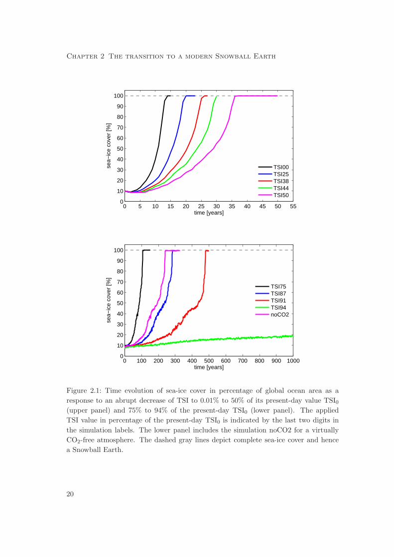
Figure 2.1: Time evolution of sea-ice cover in percentage of global ocean area as a
response to an abrupt decrease of TSI to 0.01% to 50% of its present-day value TSI0(upper panel) and 75% to 94% of the present-day TSI0 (lower panel). The applied
TSI value in percentage of the present-day TSI0 is indicated by the last two digits in
the simulation labels. The lower panel includes the simulation noCO2 for a virtually
CO2-free atmosphere. The dashed gray lines depict complete sea-ice cover and hence
a Snowball Earth.
20
2.4 Snowball Earth bifurcation point and transition time
the Pacific, with the time lag increasing from 3 months for the simulation TSI00 to 10
years for the simulation TSI91. Sea ice quickly becomes covered with snow, causing an
albedo increase compared to bare sea ice by up to 0.1 in all simulations. In contrast,
the formation of snow on land depends strongly on the TSI reduction. For simulations
with drastic TSI reductions and hence shorter transition times, land snow cover is
more spatially homogeneous but reaches lower maximum values. For example, land
snow cover at the end of simulation TSI00 exceeds 0.2 m water equivalent everywhere
except in the the tropical regions of Africa, South America and China, whereas at the
end of simulation TSI91, most land areas show no or only little snow cover (below
0.05 m water equivalent), and heavy snow cover of water equivalents of 1 m or more is
restricted to the Himalaya, the Rocky Mountains, the Andes, and tropical Africa.
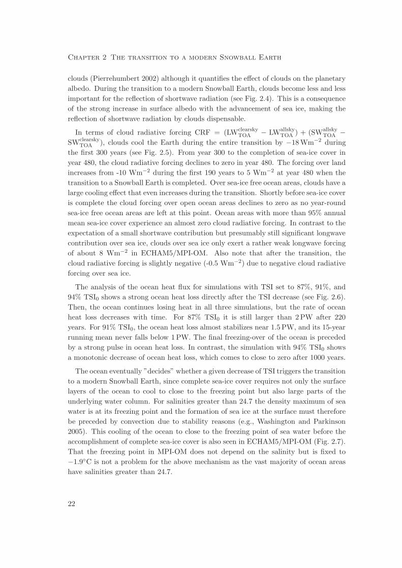
We now analyze the role of clouds and water vapor during the transition to a modern
Snowball Earth as modelled in simulation TSI91. In the case of longwave radiation we
can disentangle the radiative effect of clouds from the effect of water vapor by means
of the all-sky and clear-sky radiation fluxes at the top of the atmosphere. These are
simultaneously calculated in ECHAM5. During the transition the effective surface
emissivity ǫ, defined as the ratio of outgoing all-sky longwave radiation at the top
of atmosphere and the upward longwave radiation emitted by the Earth’s surface,
increases from 0.6 to 0.86, meaning a strong decline of the greenhouse effect, g = 1− ǫ,
with the cooling of the Earth. The longwave effect of water vapour (ǫclearsky) can be
disentangled from the effect of clouds (ǫclouds) by
ǫ = ǫclearsky + ǫclouds = LWallskyTOA /LW↑,surface (2.1)
with
ǫclearsky = LWclearskyTOA /LW↑,surface. (2.2)
Here, LWTOA denotes the globally averaged annual longwave radiation at the top of
the atmosphere with the superscripts marking the all-sky and the clear-sky fluxes.
LW↑,surface labels the globally averaged annual upward longwave radiation at the Earth’s
surface. Fig. 2.2 shows that the effect of clouds on the effective surface emissivity stays
constant during the entire transition to a modern Snowball Earth. The increase in
the effective surface emissivity is indeed entirely caused by the increase in the clear-sky
surface emissivity itself resulting from the decrease in atmospheric water vapour content
(see Fig. 2.3). We also find the logarithmic dependence of the clear-sky greenhouse effect
gclearsky = 1−ǫclearsky on the atmospheric water vapour content (Raval and Ramanathan
1989) over the whole range of water vapour content from 0.3 to 18 kgm−2 (not shown).
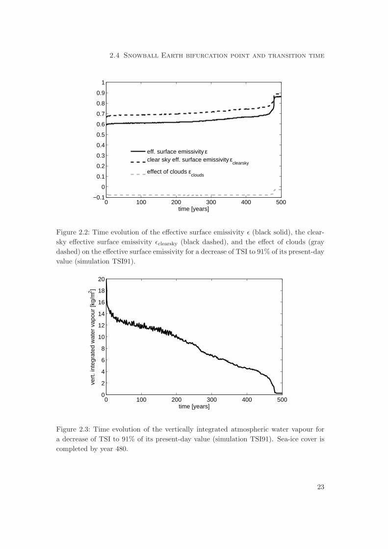
In the case of shortwave radiation the effect of clouds can be characterized by the
difference of the all-sky planetary albedo αallsky = SWallsky↑,TOA/SW↓,TOA and the clear-
sky planetary albedo αclearsky = SWclearsky↑,TOA /SW↓,TOA, with the indices having the same
meaning as in (2.1) and (2.2). Note that this difference is not equal to the albedo of
21
Chapter 2 The transition to a modern Snowball Earth
clouds (Pierrehumbert 2002) although it quantifies the effect of clouds on the planetary
albedo. During the transition to a modern Snowball Earth, clouds become less and less
important for the reflection of shortwave radiation (see Fig. 2.4). This is a consequence
of the strong increase in surface albedo with the advancement of sea ice, making the
reflection of shortwave radiation by clouds dispensable.
In terms of cloud radiative forcing CRF = (LWclearskyTOA − LWallsky
TOA ) + (SWallskyTOA −
SWclearskyTOA ), clouds cool the Earth during the entire transition by −18 Wm−2 during
the first 300 years (see Fig. 2.5). From year 300 to the completion of sea-ice cover in
year 480, the cloud radiative forcing declines to zero in year 480. The forcing over land
increases from -10 Wm−2 during the first 190 years to 5 Wm−2 at year 480 when the
transition to a Snowball Earth is completed. Over sea-ice free ocean areas, clouds have a
large cooling effect that even increases during the transition. Shortly before sea-ice cover
is complete the cloud forcing over open ocean areas declines to zero as no year-round
sea-ice free ocean areas are left at this point. Ocean areas with more than 95% annual
mean sea-ice cover experience an almost zero cloud radiative forcing. In contrast to the
expectation of a small shortwave contribution but presumably still significant longwave
contribution over sea ice, clouds over sea ice only exert a rather weak longwave forcing
of about 8 Wm−2 in ECHAM5/MPI-OM. Also note that after the transition, the
cloud radiative forcing is slightly negative (-0.5 Wm−2) due to negative cloud radiative
forcing over sea ice.
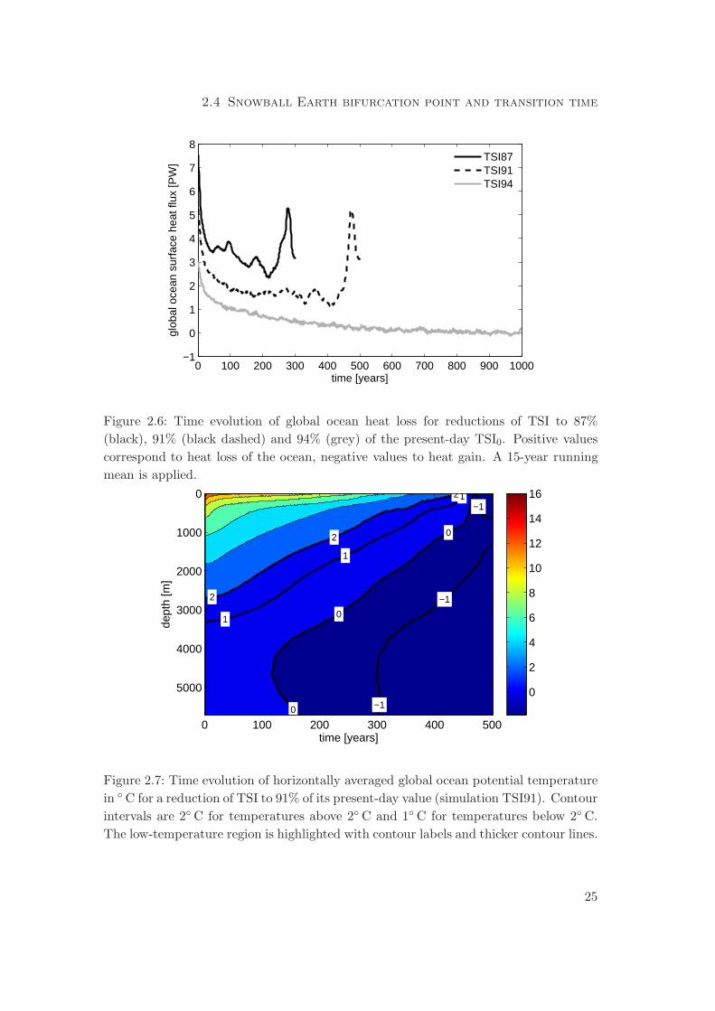
The analysis of the ocean heat flux for simulations with TSI set to 87%, 91%, and
94% TSI0 shows a strong ocean heat loss directly after the TSI decrease (see Fig. 2.6).
Then, the ocean continues losing heat in all three simulations, but the rate of ocean
heat loss decreases with time. For 87% TSI0 it is still larger than 2 PW after 220
years. For 91% TSI0, the ocean heat loss almost stabilizes near 1.5 PW, and its 15-year
running mean never falls below 1 PW. The final freezing-over of the ocean is preceded
by a strong pulse in ocean heat loss. In contrast, the simulation with 94% TSI0 shows
a monotonic decrease of ocean heat loss, which comes to close to zero after 1000 years.
The ocean eventually ”decides” whether a given decrease of TSI triggers the transition
to a modern Snowball Earth, since complete sea-ice cover requires not only the surface
layers of the ocean to cool to close to the freezing point but also large parts of the
underlying water column. For salinities greater than 24.7 the density maximum of sea
water is at its freezing point and the formation of sea ice at the surface must therefore
be preceded by convection due to stability reasons (e.g., Washington and Parkinson
2005). This cooling of the ocean to close to the freezing point of sea water before the
accomplishment of complete sea-ice cover is also seen in ECHAM5/MPI-OM (Fig. 2.7).
That the freezing point in MPI-OM does not depend on the salinity but is fixed to
−1.9◦C is not a problem for the above mechanism as the vast majority of ocean areas
have salinities greater than 24.7.
22
2.4 Snowball Earth bifurcation point and transition time
0 100 200 300 400 500−0.1
0
0.1
0.2
0.3
0.4
0.5
0.6
0.7
0.8
0.9
1
time [years]
eff. surface emissivity εclear sky eff. surface emissivity ε
clearsky
effect of clouds εclouds
Figure 2.2: Time evolution of the effective surface emissivity ǫ (black solid), the clear-
sky effective surface emissivity ǫclearsky (black dashed), and the effect of clouds (gray
dashed) on the effective surface emissivity for a decrease of TSI to 91% of its present-day
value (simulation TSI91).
0 100 200 300 400 5000
2
4
6
8
10
12
14
16
18
20
time [years]
vert
. int
egra
ted
wat
er v
apou
r [k
g/m
2 ]
Figure 2.3: Time evolution of the vertically integrated atmospheric water vapour for
a decrease of TSI to 91% of its present-day value (simulation TSI91). Sea-ice cover is
completed by year 480.
23
Chapter 2 The transition to a modern Snowball Earth
0 100 200 300 400 5000
0.1
0.2
0.3
0.4
0.5
0.6
0.7
0.8
time [years]
planetary albedo αclear sky planetary albedo α
clearsky
contribution of clouds to plan. albedo
Figure 2.4: Time evolution of planetary albedo (black solid), clear-sky planetary albedo
(black dashed), and the effect of clouds on the planetary albedo as characterized by the
difference of the planetary albedo and the clear-sky planetary albedo (gray dashed),
for a decrease of TSI to 91% of its present-day value (simulation TSI91).
0 100 200 300 400 500−50
−40
−30
−20
−10
0
10
time [ years]
clou
d ra
diat
ive
forc
ing
[Wm
−2 ]
totallandoceansea ice
Figure 2.5: Time evolution of the cloud radiative forcing for a decrease of TSI to 91% of
its present-day value (simulation TSI91). Sea-ice cover is completed by year 480. When
calculating the individual contribution of land, ocean and sea-ice areas, we dismissed
”mixed” land-ocean cells. For the cloud radiative forcing over ocean areas, we only
considered ocean cells with zero annual mean sea-ice cover. For the cloud radiative
forcing over sea-ice areas, we only considered ocean cells with annual mean sea-ice
cover greater than 95%.
24
2.4 Snowball Earth bifurcation point and transition time
0 100 200 300 400 500 600 700 800 900 1000−1
0
1
2
3
4
5
6
7
8
time [years]
glob
al o
cean
sur
face
hea
t flu
x [P
W]
TSI87TSI91TSI94
Figure 2.6: Time evolution of global ocean heat loss for reductions of TSI to 87%
(black), 91% (black dashed) and 94% (grey) of the present-day TSI0. Positive values
correspond to heat loss of the ocean, negative values to heat gain. A 15-year running
mean is applied.
time [years]
dept
h [m
]
−1
−1
−1
0
0
0
1
1
1
2
2
2
0 100 200 300 400 500
0
1000
2000
3000
4000
5000 0
2
4
6
8
10
12
14
16
Figure 2.7: Time evolution of horizontally averaged global ocean potential temperature
in ◦ C for a reduction of TSI to 91% of its present-day value (simulation TSI91). Contour
intervals are 2◦ C for temperatures above 2◦ C and 1◦ C for temperatures below 2◦ C.
The low-temperature region is highlighted with contour labels and thicker contour lines.
25
Chapter 2 The transition to a modern Snowball Earth
2.5 Comparison to a zero-dimensional energy balance model
of mean ocean potential temperature
The ocean is by far the largest heat reservoir of the climate system and has to cool
down to close to the freezing point before a modern Snowball Earth is possible. In the
light of this outstanding role of the ocean, we devise a zero-dimensional energy balance
model of the mean ocean potential temperature (shortly called energy balance model in
the following). By modelling the response of the mean ocean potential temperature to
a decrease in total solar irradiance, this energy balance model will allow us to estimate
the transition time from the present-day climate to a modern Snowball Earth as well
as the Snowball Earth bifurcation point.
We assume that the ocean is perfectly mixed in both the horizontal and the vertical
directions. While this assumption is clearly daring for the present-day ocean, it becomes
more and more reasonable as the Earth’s climate approaches the Snowball Earth as
described at the end of the preceding section. The energy balance model neglects the
heat stored in the atmosphere and land components of the climate system.
In the energy balance model the heat flux at the ocean’s surface is described by
the (im)balance of shortwave and longwave radiation, and the mean ocean potential
temperature (referred to as ocean temperature in the following), θ, consequently obeys
the budget equation
cdθ
dt=
(1 − α)
4TSI − ǫσθ4, (2.3)
with c denoting the specific heat capacity of the ocean per unit area. Based on the
MPI-OM parameters for the specific heat capacity of sea water, the density of sea water,
and the global ocean volume and surface area, we obtain c = 1.53 · 1010 JK−1m−2. The
exact value of c is not at all crucial for the results of the energy balance model though it
ensures that the two tuning parameters α and ǫ take reasonable values. The parameter
α models the reflection of solar radiation by clouds and by the ocean’s surface and
hence can be thought of as the planetary albedo. The parameter ǫ can be thought of as
the effective surface emissivity and hence the efficiency of ocean heat loss by longwave
radiation.
We use this energy balance model to predict the time evolution of the ocean temper-
ature θ after an abrupt decrease of TSI. The model is only valid for ocean temperatures
above the freezing temperature of sea water θf = −1.9◦ C. This is enough for our pur-
poses here since we are only interested in the transition to a modern Snowball Earth,
which in the energy balance model is defined by θ = θf . The temperature of the
present-day ocean is diagnosed from the control simulation CTRL to be θpd = 4.35◦C
and is used as the initial condition to (2.3). Requiring that the present-day ocean is an
equilibrium solution of (2.3) for the present-day TSI0 = 1367 Wm−2, the ratio of the
26
2.5 Comparison to a 0-d EBM
two tuning parameters α and ǫ is fixed to
(1 − α)
ǫ= 4σ
θ4pd
TSI0≃ 0.9838. (2.4)
The value of ǫ is determined by demanding that the energy balance model matches
the transition time of 14 years found in the ECHAM5/MPI-OM simulation TSI00. In
this case, the solar radiation term in (2.3) can be neglected, and in conjunction with
the initial condition θ = θpd and the constraint θ = θf for t = 14 years, we arrive at
ǫ = 0.6736. This fitted value of ǫ is taken to be constant for all TSI values. With (2.4) it
follows that α = 0.3373. In contrast to the energy balance models of Budyko and Sellers
the albedo is held constant for all ocean temperatures between the freezing temperature
of sea water and the present-day ocean temperature. Although we thus do not allow
for an ice-albedo feedback in our energy balance model, this has the advantage that
the estimate of the Snowball Earth bifurcation point gained with our energy balance
model does not dependent on a chosen albedo parametrization as in the Budyko-Sellers
models.
The fitted albedo of the energy balance model is close to the present-day plane-
tary albedo, αpd, which is estimated in the ECHAM5/MPI-OM control simulation
CTRL to αpd = 0.326. When comparing the effective surface emissivity of the energy
balance model to the present-day effective surface emissivity ǫpd as modeled in the
ECHAM5/MPI-OM control simulation CTRL, we need to include a form factor in ǫpd
to incorporate that the sea surface temperature is larger than the vertically averaged
mean ocean potential temperature used in the energy balance model to describe the
energy loss by longwave radiation. With a present-day mean sea surface temperature
of SSTpd = 11.31◦C, a present-day mean ocean potential temperature θpd = 4.35◦C,
and a present-day mean effective surface emissivity ǫpd = 0.583 as estimated in the
ECHAM5/MPI-OM control simulation CTRL, we arrive at a ”corrected” value for the
present-day effective surface emissivity of ǫcorrpd = ǫpd(SSTpd/θpd)4 = 0.644 (with both
SSTpd and θpd given in Kelvin). As for the albedo the effective surface emissivity of
the energy balance model is thus close to its present-day value though slightly larger.
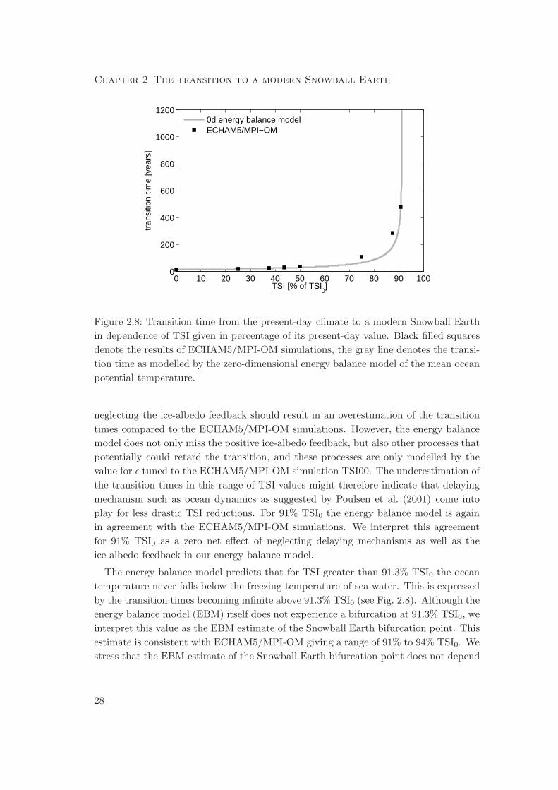
With these choices for α and ǫ, we use the energy balance model to estimate the
transition time to a Snowball Earth as a function of decrease in TSI. This is done by
solving (2.3) with the initial condition θ = θpd and the final condition θ = θf . The
resulting transition times are shown in Fig. 2.8 (gray line), which also includes the
transition times found by the ECHAM5/MPI-OM simulations (black filled squares).
The energy balance model is in good agreement with the ECHAM5/MPI-OM results
for TSI values in the range of 0% to 50% TSI0. This shows that TSI reductions to less
than 50% are well described by radiative cooling of the ocean. In contrast, the energy
balance model underestimates the transition times for the two TSI values 75% TSI0 and
87% TSI0. This underestimation is somewhat surprising since one would expect that
27
Chapter 2 The transition to a modern Snowball Earth
0 10 20 30 40 50 60 70 80 90 1000
200
400
600
800
1000
1200
TSI [% of TSI0]
tran
sitio
n tim
e [y
ears
]
0d energy balance modelECHAM5/MPI−OM
Figure 2.8: Transition time from the present-day climate to a modern Snowball Earth
in dependence of TSI given in percentage of its present-day value. Black filled squares
denote the results of ECHAM5/MPI-OM simulations, the gray line denotes the transi-
tion time as modelled by the zero-dimensional energy balance model of the mean ocean
potential temperature.
neglecting the ice-albedo feedback should result in an overestimation of the transition
times compared to the ECHAM5/MPI-OM simulations. However, the energy balance
model does not only miss the positive ice-albedo feedback, but also other processes that
potentially could retard the transition, and these processes are only modelled by the
value for ǫ tuned to the ECHAM5/MPI-OM simulation TSI00. The underestimation of
the transition times in this range of TSI values might therefore indicate that delaying
mechanism such as ocean dynamics as suggested by Poulsen et al. (2001) come into
play for less drastic TSI reductions. For 91% TSI0 the energy balance model is again
in agreement with the ECHAM5/MPI-OM simulations. We interpret this agreement
for 91% TSI0 as a zero net effect of neglecting delaying mechanisms as well as the
ice-albedo feedback in our energy balance model.
The energy balance model predicts that for TSI greater than 91.3% TSI0 the ocean
temperature never falls below the freezing temperature of sea water. This is expressed
by the transition times becoming infinite above 91.3% TSI0 (see Fig. 2.8). Although the
energy balance model (EBM) itself does not experience a bifurcation at 91.3% TSI0, we
interpret this value as the EBM estimate of the Snowball Earth bifurcation point. This
estimate is consistent with ECHAM5/MPI-OM giving a range of 91% to 94% TSI0. We
stress that the EBM estimate of the Snowball Earth bifurcation point does not depend
28
2.6 Atmosphere and ocean circulations and heat transports
on the individual values for α and ǫ, but only on their ratio in (2.4). On the one hand,
this means that we could also tune α and ǫ to any ECHAM5/MPI-OM simulation
with a TSI reduction below or equal to 91% TSI0 without changing the EBM estimate
of the Snowball Earth bifurcation point. On the other hand, if we chose a larger
ratio, or equivalently a larger present-day ocean temperature θpd, the EBM estimate
of the Snowball Earth bifurcation point would shift towards lower TSI. Therefore the
present-day climate, represented in the energy balance model by the present-day ocean
temperature, entirely controls the EBM estimate of the Snowball Earth bifurcation
point through (2.4).
2.6 Atmosphere and ocean circulations and heat transports
We now study the atmosphere and ocean circulations both for a climate with extended
but not complete sea-ice cover and for the entire transition period to a modern Snow-
ball Earth. The focus will be on the Hadley cell in the atmosphere and the Atlantic
meridional overturning circulation (AMOC). We also investigate atmosphere and ocean
meridional heat transports and analyze how they are related to changes in the mean
meridional circulations. For the atmosphere, we analyze the total advective heat trans-
port and its decomposition in mean meridional and eddy transports. We use six-hourly
instantaneous data and define the eddy terms as the deviation from the monthly and
zonal mean. For the ocean, we report on the total ocean heat transport (calculated as
the implied ocean heat transport based on monthly data of the heat and water fluxes at
the ocean surface as well as monthly data of the ocean potential temperature) and the
contribution of the meridional overturning circulation (calculated by monthly data of
the horizontal velocity field and the ocean potential temperature). Moreover, we study
the transport of latent heat due to sea-ice dynamics, which we calculate as the product
of the transported sea-ice volume times the melting enthalpy of sea-ice of 320·106 Jm−3.
We here analyze two simulations. First, we investigate the last 50 years of the
simulation TSI94 as representative for an equilibrium climate with extended but not
complete sea-ice cover. Second, we study the transient simulation TSI91 from the
abrupt decrease of TSI to 91% until completion of sea-ice cover after 480 years.
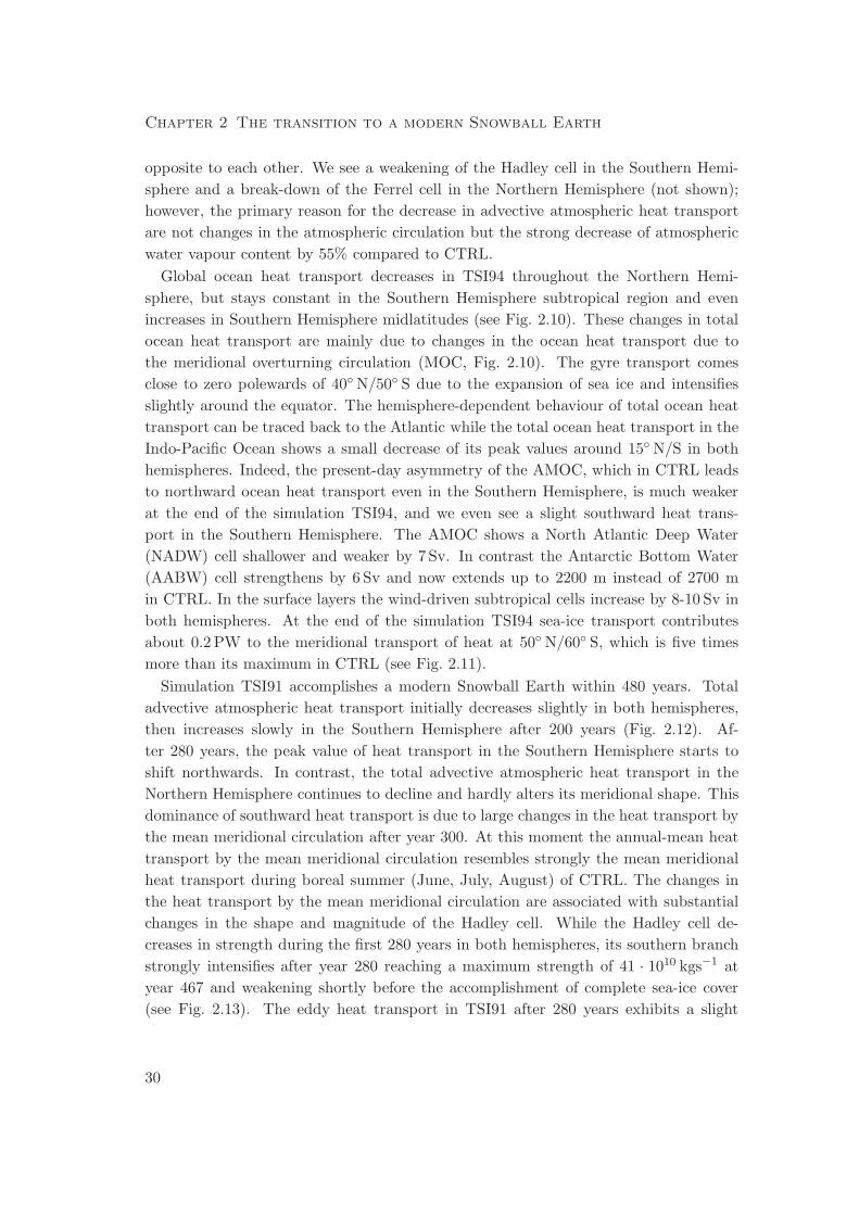
We start with the analysis of the last 50 years of the simulation TSI94. The total ad-
vective atmospheric heat transport shown in Fig. 2.9 decreases in the Southern as well
as the Northern Hemisphere with a decrease of the maximum heat transport around
35◦ N/S by 0.8 PW. This decrease is mainly due to a decrease of eddy transport around
35◦ N/S, which is caused by a decrease of eddy latent heat transport while the eddy
dry static heat transport is virtually unchanged compared to the control simulation
(not shown). The total heat transport by the mean meridional circulation changes very
little, but this is a zero net effect of strong decreases in the magnitudes of the dry static
heat transport and latent heat transport by the mean meridional circulation, which are
29
Chapter 2 The transition to a modern Snowball Earth
opposite to each other. We see a weakening of the Hadley cell in the Southern Hemi-
sphere and a break-down of the Ferrel cell in the Northern Hemisphere (not shown);
however, the primary reason for the decrease in advective atmospheric heat transport
are not changes in the atmospheric circulation but the strong decrease of atmospheric
water vapour content by 55% compared to CTRL.
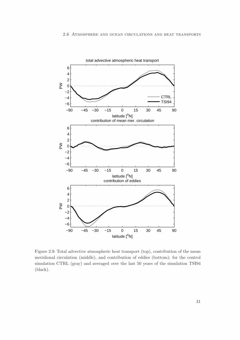
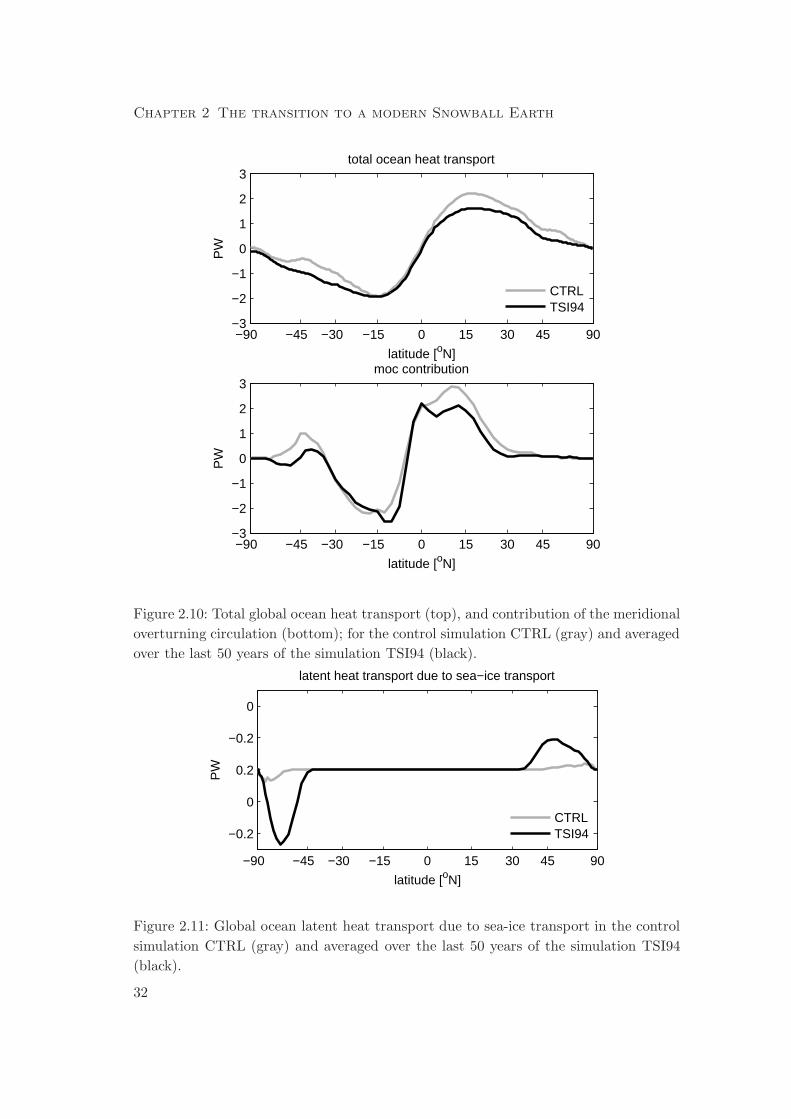
Global ocean heat transport decreases in TSI94 throughout the Northern Hemi-
sphere, but stays constant in the Southern Hemisphere subtropical region and even
increases in Southern Hemisphere midlatitudes (see Fig. 2.10). These changes in total
ocean heat transport are mainly due to changes in the ocean heat transport due to
the meridional overturning circulation (MOC, Fig. 2.10). The gyre transport comes
close to zero polewards of 40◦ N/50◦ S due to the expansion of sea ice and intensifies
slightly around the equator. The hemisphere-dependent behaviour of total ocean heat
transport can be traced back to the Atlantic while the total ocean heat transport in the
Indo-Pacific Ocean shows a small decrease of its peak values around 15◦ N/S in both
hemispheres. Indeed, the present-day asymmetry of the AMOC, which in CTRL leads
to northward ocean heat transport even in the Southern Hemisphere, is much weaker
at the end of the simulation TSI94, and we even see a slight southward heat trans-
port in the Southern Hemisphere. The AMOC shows a North Atlantic Deep Water
(NADW) cell shallower and weaker by 7 Sv. In contrast the Antarctic Bottom Water
(AABW) cell strengthens by 6 Sv and now extends up to 2200 m instead of 2700 m
in CTRL. In the surface layers the wind-driven subtropical cells increase by 8-10 Sv in
both hemispheres. At the end of the simulation TSI94 sea-ice transport contributes
about 0.2 PW to the meridional transport of heat at 50◦ N/60◦ S, which is five times
more than its maximum in CTRL (see Fig. 2.11).
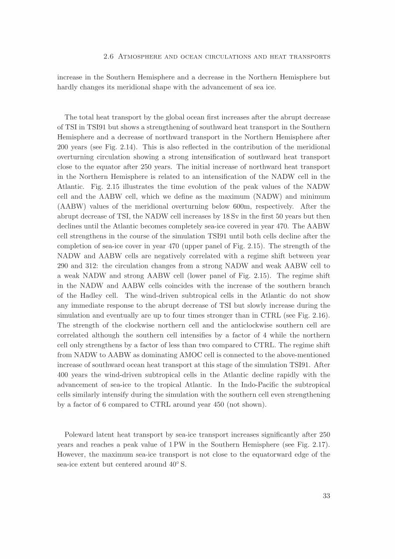
Simulation TSI91 accomplishes a modern Snowball Earth within 480 years. Total
advective atmospheric heat transport initially decreases slightly in both hemispheres,
then increases slowly in the Southern Hemisphere after 200 years (Fig. 2.12). Af-
ter 280 years, the peak value of heat transport in the Southern Hemisphere starts to
shift northwards. In contrast, the total advective atmospheric heat transport in the
Northern Hemisphere continues to decline and hardly alters its meridional shape. This
dominance of southward heat transport is due to large changes in the heat transport by
the mean meridional circulation after year 300. At this moment the annual-mean heat
transport by the mean meridional circulation resembles strongly the mean meridional
heat transport during boreal summer (June, July, August) of CTRL. The changes in
the heat transport by the mean meridional circulation are associated with substantial
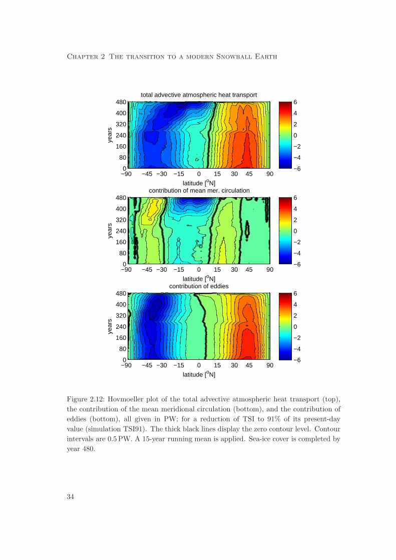
changes in the shape and magnitude of the Hadley cell. While the Hadley cell de-
creases in strength during the first 280 years in both hemispheres, its southern branch
strongly intensifies after year 280 reaching a maximum strength of 41 · 1010 kgs−1 at
year 467 and weakening shortly before the accomplishment of complete sea-ice cover
(see Fig. 2.13). The eddy heat transport in TSI91 after 280 years exhibits a slight
30
2.6 Atmosphere and ocean circulations and heat transports
−90 −45 −30 −15 0 15 30 45 90
−6
−4
−2
0
2
4
6
latitude [oN]
PW
total advective atmospheric heat transport
CTRLTSI94
−90 −45 −30 −15 0 15 30 45 90
−6
−4
−2
0
2
4
6
latitude [oN]
PW
contribution of mean mer. circulation
−90 −45 −30 −15 0 15 30 45 90
−6
−4
−2
0
2
4
6
latitude [oN]
PW
contribution of eddies
Figure 2.9: Total advective atmospheric heat transport (top), contribution of the mean
meridional circulation (middle), and contribution of eddies (bottom); for the control
simulation CTRL (gray) and averaged over the last 50 years of the simulation TSI94
(black).
31
Chapter 2 The transition to a modern Snowball Earth
−90 −45 −30 −15 0 15 30 45 90−3
−2
−1
0
1
2
3
latitude [oN]
PW
total ocean heat transport
CTRLTSI94
−90 −45 −30 −15 0 15 30 45 90−3
−2
−1
0
1
2
3
latitude [oN]
PW
moc contribution
Figure 2.10: Total global ocean heat transport (top), and contribution of the meridional
overturning circulation (bottom); for the control simulation CTRL (gray) and averaged
over the last 50 years of the simulation TSI94 (black).
−90 −45 −30 −15 0 15 30 45 90
−0.2
0
0.2
−0.2
0
latitude [oN]
PW
latent heat transport due to sea−ice transport
CTRLTSI94
Figure 2.11: Global ocean latent heat transport due to sea-ice transport in the control
simulation CTRL (gray) and averaged over the last 50 years of the simulation TSI94
(black).
32
2.6 Atmosphere and ocean circulations and heat transports
increase in the Southern Hemisphere and a decrease in the Northern Hemisphere but
hardly changes its meridional shape with the advancement of sea ice.
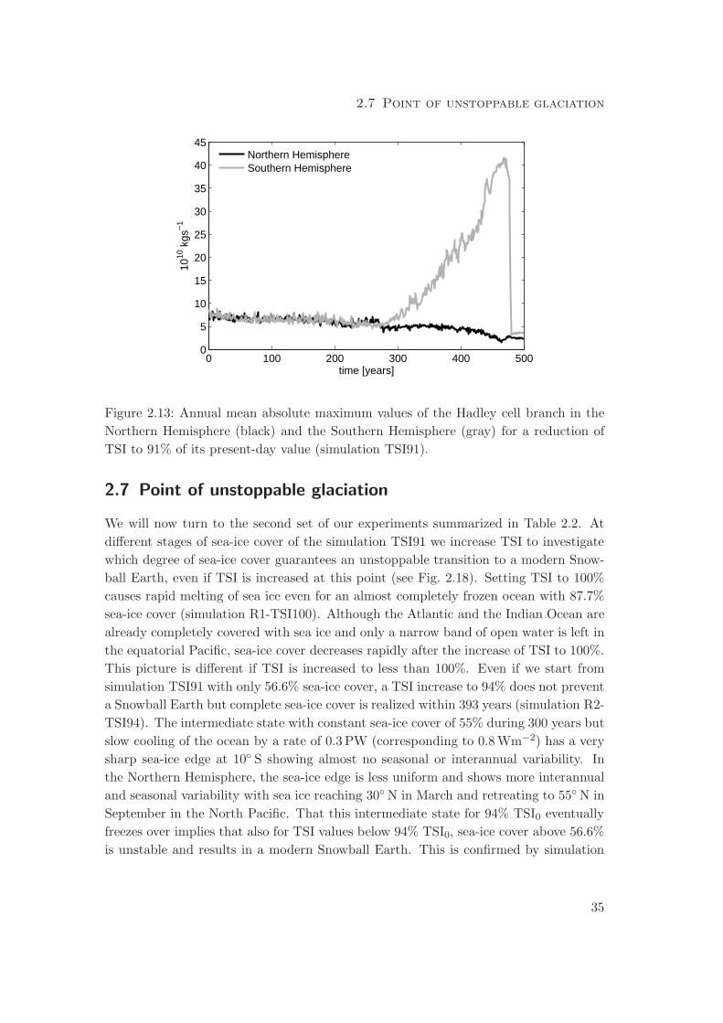
The total heat transport by the global ocean first increases after the abrupt decrease
of TSI in TSI91 but shows a strengthening of southward heat transport in the Southern
Hemisphere and a decrease of northward transport in the Northern Hemisphere after
200 years (see Fig. 2.14). This is also reflected in the contribution of the meridional
overturning circulation showing a strong intensification of southward heat transport
close to the equator after 250 years. The initial increase of northward heat transport
in the Northern Hemisphere is related to an intensification of the NADW cell in the
Atlantic. Fig. 2.15 illustrates the time evolution of the peak values of the NADW
cell and the AABW cell, which we define as the maximum (NADW) and minimum
(AABW) values of the meridional overturning below 600m, respectively. After the
abrupt decrease of TSI, the NADW cell increases by 18 Sv in the first 50 years but then
declines until the Atlantic becomes completely sea-ice covered in year 470. The AABW
cell strengthens in the course of the simulation TSI91 until both cells decline after the
completion of sea-ice cover in year 470 (upper panel of Fig. 2.15). The strength of the
NADW and AABW cells are negatively correlated with a regime shift between year
290 and 312: the circulation changes from a strong NADW and weak AABW cell to
a weak NADW and strong AABW cell (lower panel of Fig. 2.15). The regime shift
in the NADW and AABW cells coincides with the increase of the southern branch
of the Hadley cell. The wind-driven subtropical cells in the Atlantic do not show
any immediate response to the abrupt decrease of TSI but slowly increase during the
simulation and eventually are up to four times stronger than in CTRL (see Fig. 2.16).
The strength of the clockwise northern cell and the anticlockwise southern cell are
correlated although the southern cell intensifies by a factor of 4 while the northern
cell only strengthens by a factor of less than two compared to CTRL. The regime shift
from NADW to AABW as dominating AMOC cell is connected to the above-mentioned
increase of southward ocean heat transport at this stage of the simulation TSI91. After
400 years the wind-driven subtropical cells in the Atlantic decline rapidly with the
advancement of sea-ice to the tropical Atlantic. In the Indo-Pacific the subtropical
cells similarly intensify during the simulation with the southern cell even strengthening
by a factor of 6 compared to CTRL around year 450 (not shown).
Poleward latent heat transport by sea-ice transport increases significantly after 250
years and reaches a peak value of 1PW in the Southern Hemisphere (see Fig. 2.17).
However, the maximum sea-ice transport is not close to the equatorward edge of the
sea-ice extent but centered around 40◦ S.
33
Chapter 2 The transition to a modern Snowball Earth
latitude [oN]
year
s
total advective atmospheric heat transport
−90 −45 −30 −15 0 15 30 45 900
80
160
240
320
400
480
−6
−4
−2
0
2
4
6
latitude [oN]
year
s
contribution of mean mer. circulation
−90 −45 −30 −15 0 15 30 45 900
80
160
240
320
400
480
−6
−4
−2
0
2
4
6
latitude [oN]
year
s
contribution of eddies
−90 −45 −30 −15 0 15 30 45 900
80
160
240
320
400
480
−6
−4
−2
0
2
4
6
Figure 2.12: Hovmoeller plot of the total advective atmospheric heat transport (top),
the contribution of the mean meridional circulation (bottom), and the contribution of
eddies (bottom), all given in PW; for a reduction of TSI to 91% of its present-day
value (simulation TSI91). The thick black lines display the zero contour level. Contour
intervals are 0.5 PW. A 15-year running mean is applied. Sea-ice cover is completed by
year 480.
34
2.7 Point of unstoppable glaciation
0 100 200 300 400 5000
5
10
15
20
25
30
35
40
45
time [years]
1010
kgs
−1
Northern HemisphereSouthern Hemisphere
Figure 2.13: Annual mean absolute maximum values of the Hadley cell branch in the
Northern Hemisphere (black) and the Southern Hemisphere (gray) for a reduction of
TSI to 91% of its present-day value (simulation TSI91).
2.7 Point of unstoppable glaciation
We will now turn to the second set of our experiments summarized in Table 2.2. At
different stages of sea-ice cover of the simulation TSI91 we increase TSI to investigate
which degree of sea-ice cover guarantees an unstoppable transition to a modern Snow-
ball Earth, even if TSI is increased at this point (see Fig. 2.18). Setting TSI to 100%
causes rapid melting of sea ice even for an almost completely frozen ocean with 87.7%
sea-ice cover (simulation R1-TSI100). Although the Atlantic and the Indian Ocean are
already completely covered with sea ice and only a narrow band of open water is left in
the equatorial Pacific, sea-ice cover decreases rapidly after the increase of TSI to 100%.
This picture is different if TSI is increased to less than 100%. Even if we start from
simulation TSI91 with only 56.6% sea-ice cover, a TSI increase to 94% does not prevent
a Snowball Earth but complete sea-ice cover is realized within 393 years (simulation R2-
TSI94). The intermediate state with constant sea-ice cover of 55% during 300 years but
slow cooling of the ocean by a rate of 0.3 PW (corresponding to 0.8 Wm−2) has a very
sharp sea-ice edge at 10◦ S showing almost no seasonal or interannual variability. In
the Northern Hemisphere, the sea-ice edge is less uniform and shows more interannual
and seasonal variability with sea ice reaching 30◦ N in March and retreating to 55◦ N in
September in the North Pacific. That this intermediate state for 94% TSI0 eventually
freezes over implies that also for TSI values below 94% TSI0, sea-ice cover above 56.6%
is unstable and results in a modern Snowball Earth. This is confirmed by simulation
35
Chapter 2 The transition to a modern Snowball Earth
latitude [oN]
year
s
total global ocean heat transport
−90 −45 −30 −15 0 15 30 45 900
80
160
240
320
400
480
−4
−2
0
2
4
latitude [oN]
year
s
moc contribution
−90 −45 −30 −15 0 15 30 45 900
80
160
240
320
400
480
−4
−2
0
2
4
Figure 2.14: Hovmoeller plot of the total global ocean heat transport (top), and the
contribution by the MOC (bottom), both given in PW; for a reduction of TSI to 91% of
its present-day value (simulation TSI91). The thick black lines display the zero contour
level. Contour intervals are 0.5 PW. A 15-year running mean is applied. Sea-ice cover
is completed by year 480.
36
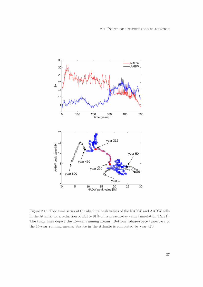
2.7 Point of unstoppable glaciation
0 100 200 300 400 5000
5
10
15
20
25
30
35
time [years]
Sv
NADWAABW
0 5 10 15 20 25 300
4
8
12
16
20
year 500
year 312
year 470
year 1
year 50
year 290
NADW peak value [Sv]
AA
BW
pea
k va
lue
[Sv]
Figure 2.15: Top: time series of the absolute peak values of the NADW and AABW cells
in the Atlantic for a reduction of TSI to 91% of its present-day value (simulation TSI91).
The thick lines depict the 15-year running means. Bottom: phase-space trajectory of
the 15-year running means. Sea ice in the Atlantic is completed by year 470.
37
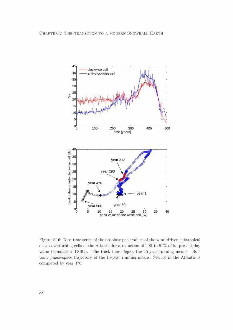
Chapter 2 The transition to a modern Snowball Earth
0 100 200 300 400 5000
5
10
15
20
25
30
35
40
45
time [years]
Sv
clockwise cellanti−clockwise cell
0 5 10 15 20 25 30 35 400
5
10
15
20
25
30
35
40
year 470
year 290
year 312
year 500
year 1
year 50
peak value of clockwise cell [Sv]
peak
val
ue o
f ant
i−cl
ockw
ise
cell
[Sv]
Figure 2.16: Top: time series of the absolute peak values of the wind-driven subtropical
ocean overturning cells of the Atlantic for a reduction of TSI to 91% of its present-day
value (simulation TSI91). The thick lines depict the 15-year running means. Bot-
tom: phase-space trajectory of the 15-year running means. Sea ice in the Atlantic is
completed by year 470.
38
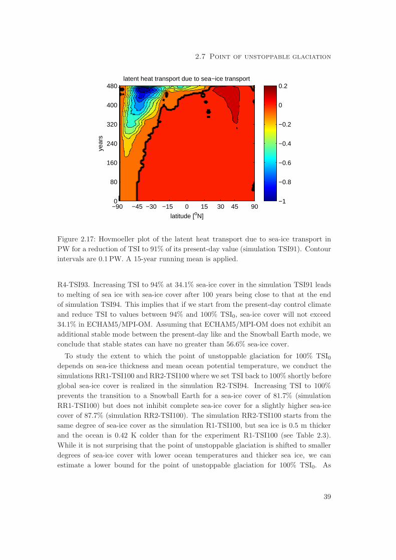
2.7 Point of unstoppable glaciation
latitude [oN]
year
s
latent heat transport due to sea−ice transport
−90 −45 −30 −15 0 15 30 45 900
80
160
240
320
400
480
−1
−0.8
−0.6
−0.4
−0.2
0
0.2
Figure 2.17: Hovmoeller plot of the latent heat transport due to sea-ice transport in
PW for a reduction of TSI to 91% of its present-day value (simulation TSI91). Contour
intervals are 0.1 PW. A 15-year running mean is applied.
R4-TSI93. Increasing TSI to 94% at 34.1% sea-ice cover in the simulation TSI91 leads
to melting of sea ice with sea-ice cover after 100 years being close to that at the end
of simulation TSI94. This implies that if we start from the present-day control climate
and reduce TSI to values between 94% and 100% TSI0, sea-ice cover will not exceed
34.1% in ECHAM5/MPI-OM. Assuming that ECHAM5/MPI-OM does not exhibit an
additional stable mode between the present-day like and the Snowball Earth mode, we
conclude that stable states can have no greater than 56.6% sea-ice cover.
To study the extent to which the point of unstoppable glaciation for 100% TSI0depends on sea-ice thickness and mean ocean potential temperature, we conduct the
simulations RR1-TSI100 and RR2-TSI100 where we set TSI back to 100% shortly before
global sea-ice cover is realized in the simulation R2-TSI94. Increasing TSI to 100%
prevents the transition to a Snowball Earth for a sea-ice cover of 81.7% (simulation
RR1-TSI100) but does not inhibit complete sea-ice cover for a slightly higher sea-ice
cover of 87.7% (simulation RR2-TSI100). The simulation RR2-TSI100 starts from the
same degree of sea-ice cover as the simulation R1-TSI100, but sea ice is 0.5 m thicker
and the ocean is 0.42 K colder than for the experiment R1-TSI100 (see Table 2.3).
While it is not surprising that the point of unstoppable glaciation is shifted to smaller
degrees of sea-ice cover with lower ocean temperatures and thicker sea ice, we can
estimate a lower bound for the point of unstoppable glaciation for 100% TSI0. As
39
Chapter 2 The transition to a modern Snowball Earth
ECHAM5/MPI-OM at the beginning of the simulation RR1-TSI100 is already close
to the maximum value of sea-ice thickness of 8 m and minimum value of mean ocean
potential temperature of −1.9◦ C, the point of unstoppable glaciation for 100% TSI0should be above 80% sea-ice cover, independent of the explicit state chosen to set TSI
back to 100%. Together with the simulations R2-TSI94 and R3-TSI94 showing that
the point of unstoppable glaciation for 94% TSI0 is below 56.6% sea-ice cover, this
demonstrates a strong dependence of the point of unstoppable glaciation on TSI.
The classical energy balance models of Budyko (1969) and Sellers (1969) describe
the climate only in terms of sea-ice cover and neglect other variables of the climate
system. This is certainly an oversimplification of the ECHAM5/MPI-OM model as
well as the ”true” climate system. We now analyze how strong this simplification
is in the case of ECHAM5/MPI-OM, by investigating the correlation of mean ocean
potential temperature and sea-ice cover for various ECHAM5/MPI-OM simulations (see
Fig. 2.19). If the energy balance models, and hence the Budyko-Sellers diagram, were
a complete description of the ECHAM5/MPI-OM model, all simulations would give
exactly the same mean ocean potential temperature for the same sea-ice cover indicating
that sea-ice cover completely describes the state of the climate system. Indeed, all
simulations of the transition from the present-day climate to a modern Snowball Earth
triggered by an abrupt decrease of TSI (cf. Tab. 2.1) roughly show the same dependence
of mean ocean potential temperature on sea-ice cover. Note that simulations of the first
set not included in Fig. 2.19 fall in the region covered by the selected simulations shown
in Fig. 2.19. This shows that sea-ice cover is a sufficient description of the climate state
of ECHAM5/MPI-OM when the climate model evolves from the present-day climate
into a modern Snowball Earth. The physical reason here is that the formation of sea
ice requires that most parts of the underlying water column are cooled to close to the
freezing point (see Sect. 2.4). In contrast, the simulation R1-TSI100 (cf. Tab. 2.2) is
not in accordance with the above correlation of mean ocean potential temperature and
sea-ice cover, because melting of sea ice only requires to warm the ocean surface layers
and hence leaves the mean ocean potential temperature largely unaffected.
2.8 Discussion
In the coupled atmosphere-ocean general circulation model ECHAM5/MPI-OM, the
Snowball Earth bifurcation point for the transition to a Snowball Earth is in the range
of 91% to 94% of today’s total solar irradiance (TSI). This is in agreement with the
FOAM atmosphere-ocean general circulation model despite differences in the applied
geography (Poulsen and Jacob 2004).
The transition times to a Snowball Earth have only been studied with a simple climate
model (Walsh and Sellers 1993); a time-dependent decrease of total solar irradiance by
30% over 90 years resulted in a Snowball Earth within 81 years. This is broadly
40
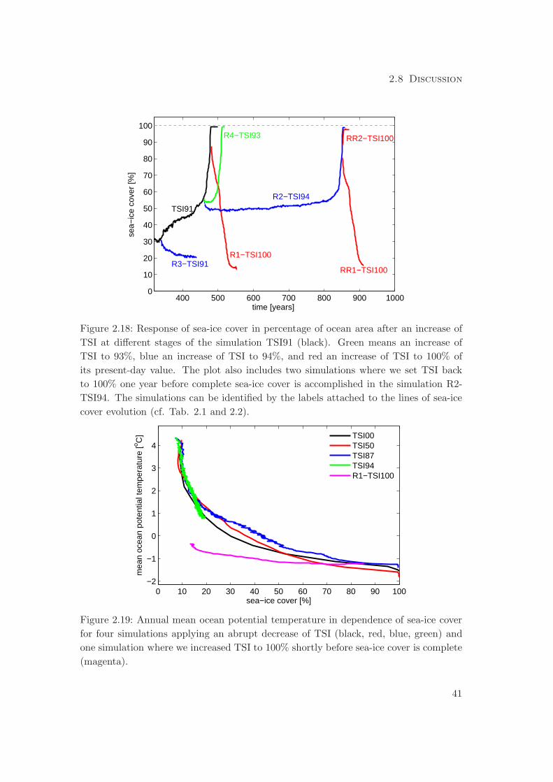
2.8 Discussion
sea−
ice
cove
r [%
]
R1−TSI100
TSI91
R4−TSI93 RR2−TSI100
RR1−TSI100
R2−TSI94
100
90
80
70
60
50
40
30
20
10
0400 500 600 700 800 900 1000
time [years]
R3−TSI91
Figure 2.18: Response of sea-ice cover in percentage of ocean area after an increase of
TSI at different stages of the simulation TSI91 (black). Green means an increase of
TSI to 93%, blue an increase of TSI to 94%, and red an increase of TSI to 100% of
its present-day value. The plot also includes two simulations where we set TSI back
to 100% one year before complete sea-ice cover is accomplished in the simulation R2-
TSI94. The simulations can be identified by the labels attached to the lines of sea-ice
cover evolution (cf. Tab. 2.1 and 2.2).
0 10 20 30 40 50 60 70 80 90 100−2
−1
0
1
2
3
4
sea−ice cover [%]
mea
n oc
ean
pote
ntia
l tem
pera
ture
[o C]
TSI00TSI50TSI87TSI94R1−TSI100
Figure 2.19: Annual mean ocean potential temperature in dependence of sea-ice cover
for four simulations applying an abrupt decrease of TSI (black, red, blue, green) and
one simulation where we increased TSI to 100% shortly before sea-ice cover is complete
(magenta).
41
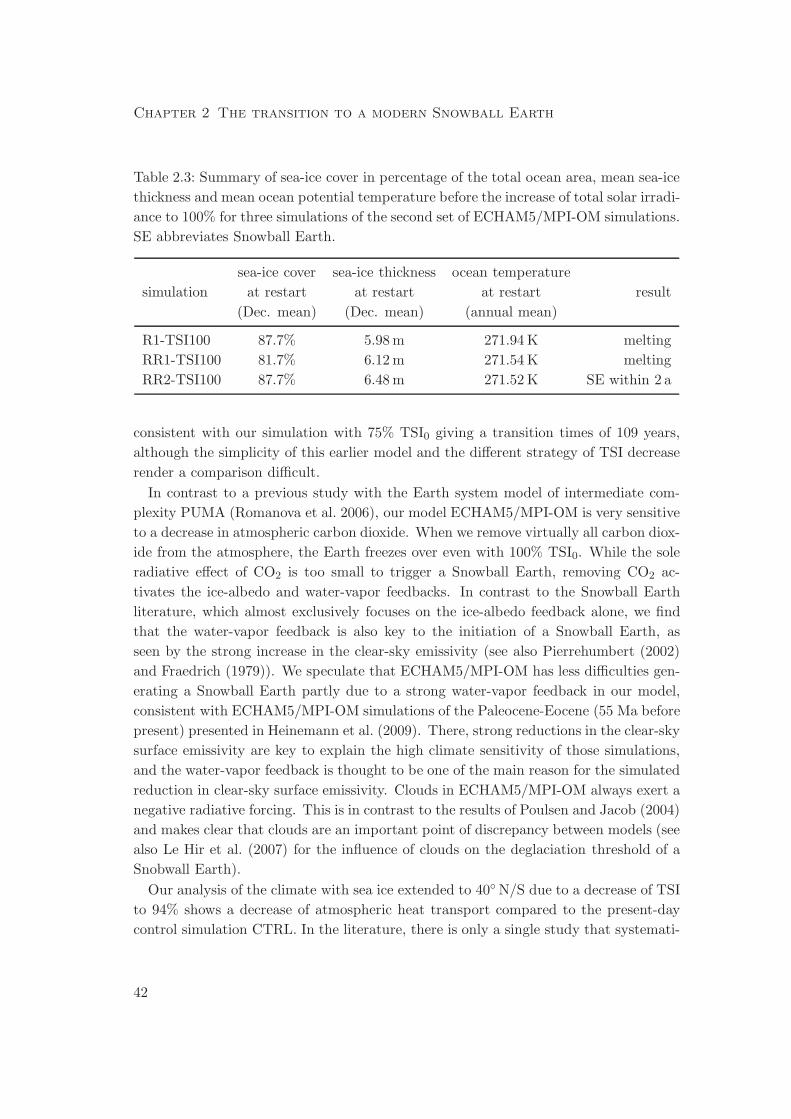
Chapter 2 The transition to a modern Snowball Earth
Table 2.3: Summary of sea-ice cover in percentage of the total ocean area, mean sea-ice
thickness and mean ocean potential temperature before the increase of total solar irradi-
ance to 100% for three simulations of the second set of ECHAM5/MPI-OM simulations.
SE abbreviates Snowball Earth.
sea-ice cover sea-ice thickness ocean temperature
simulation at restart at restart at restart result
(Dec. mean) (Dec. mean) (annual mean)
R1-TSI100 87.7% 5.98 m 271.94 K melting
RR1-TSI100 81.7% 6.12 m 271.54 K melting
RR2-TSI100 87.7% 6.48 m 271.52 K SE within 2 a
consistent with our simulation with 75% TSI0 giving a transition times of 109 years,
although the simplicity of this earlier model and the different strategy of TSI decrease
render a comparison difficult.
In contrast to a previous study with the Earth system model of intermediate com-
plexity PUMA (Romanova et al. 2006), our model ECHAM5/MPI-OM is very sensitive
to a decrease in atmospheric carbon dioxide. When we remove virtually all carbon diox-
ide from the atmosphere, the Earth freezes over even with 100% TSI0. While the sole
radiative effect of CO2 is too small to trigger a Snowball Earth, removing CO2 ac-
tivates the ice-albedo and water-vapor feedbacks. In contrast to the Snowball Earth
literature, which almost exclusively focuses on the ice-albedo feedback alone, we find
that the water-vapor feedback is also key to the initiation of a Snowball Earth, as
seen by the strong increase in the clear-sky emissivity (see also Pierrehumbert (2002)
and Fraedrich (1979)). We speculate that ECHAM5/MPI-OM has less difficulties gen-
erating a Snowball Earth partly due to a strong water-vapor feedback in our model,
consistent with ECHAM5/MPI-OM simulations of the Paleocene-Eocene (55 Ma before
present) presented in Heinemann et al. (2009). There, strong reductions in the clear-sky
surface emissivity are key to explain the high climate sensitivity of those simulations,
and the water-vapor feedback is thought to be one of the main reason for the simulated
reduction in clear-sky surface emissivity. Clouds in ECHAM5/MPI-OM always exert a
negative radiative forcing. This is in contrast to the results of Poulsen and Jacob (2004)
and makes clear that clouds are an important point of discrepancy between models (see
also Le Hir et al. (2007) for the influence of clouds on the deglaciation threshold of a
Snobwall Earth).
Our analysis of the climate with sea ice extended to 40◦ N/S due to a decrease of TSI
to 94% shows a decrease of atmospheric heat transport compared to the present-day
control simulation CTRL. In the literature, there is only a single study that systemati-
42
2.8 Discussion
cally investigates the response of atmospheric heat transport to sea-ice expansion. Using
the CLIMBER-2 model with a Neoproterozoic continental reconstruction, Donnadieu
et al. (2004b) found that a decrease of atmospheric carbon dioxide from 3500 ppm
to 500 ppm caused an expansion of sea ice from 60◦ N/S to 40◦ N/S. These simula-
tions should therefore be comparable to our present-day control simulation CTRL and
our simulation TSI94 with 94% TSI0. While in CLIMBER-2 sea-ice expansion lead
to an increase of atmospheric heat transport in both its mean meridional and eddy
components, our simulations suggest the completely opposite. We find a decrease in
atmospheric heat transport, which is entirely due to a decrease of atmospheric eddy
heat transport. This questions the conclusion in Donnadieu et al. (2004b) that atmo-
spheric heat transport represents a negative feedback working against sea-ice advance,
and illustrates that the role of atmospheric heat transport during the transition to a
Snowball Earth is still unclear. Concerning the ocean heat transport, we find similar
hemisphere-dependent changes as in Donnadieu et al. (2004b).
Why do we see an intensification of southward and a decline of northward atmospheric
and oceanic heat transports as sea ice comes close towards the equator? The answer lies
in the present-day asymmetric distribution of the continents. In ECHAM5/MPI-OM,
sea-ice covered ocean areas have a substantially higher albedo than frozen land areas
because of two reasons. First, the albedo of snow-free land largely depends on the as-
sumed background albedo, which is in the range of 0.1 to 0.3 for most land areas. This
is much lower than the albedo of sea ice. Second, snow causes less albedo increase on
land than on sea ice, since snow on land has a lower minimum albedo than snow on sea
ice, and the albedo effect of snow on land is further diminished by the shielding effect
of forests as well as the effect of decrease in fractional snow cover as a consequence
of sloping terrain. This difference in the albedo of sea-ice areas and frozen land areas
results in a larger surface albedo in the Southern than the Northern Hemisphere after
year 240 for a reduction of TSI to 91% of its present-day value (see Fig. 2.20). Conse-
quently, the Southern Hemisphere receives less shortwave radiation than the Northern
Hemisphere, and this deficit must be balanced by anomalous southward heat transport,
compared to the present-day climate. This also explains the faster expansion of sea
ice in the Southern Hemisphere seen for the simulations with 75% to 91% TSI0 (cf.,
Sect. 2.4).
How do our simulations then help us understand the role of atmosphere and ocean
heat transports and dynamics? First, we can say with confidence that the wind-driven
meridional overturning circulation intensifies strongly during the transition and hence
becomes more and more important for meridional ocean heat transport as sea ice
spreads towards the equator. This is in agreement with a previous sensitivity study with
an atmosphere-ocean general circulation model that showed that the wind-driven ocean
circulation is an important factor to make global glaciation more difficult (Poulsen and
Jacob 2004). Second, we also see the importance of sea-ice dynamics in our simulations,
43
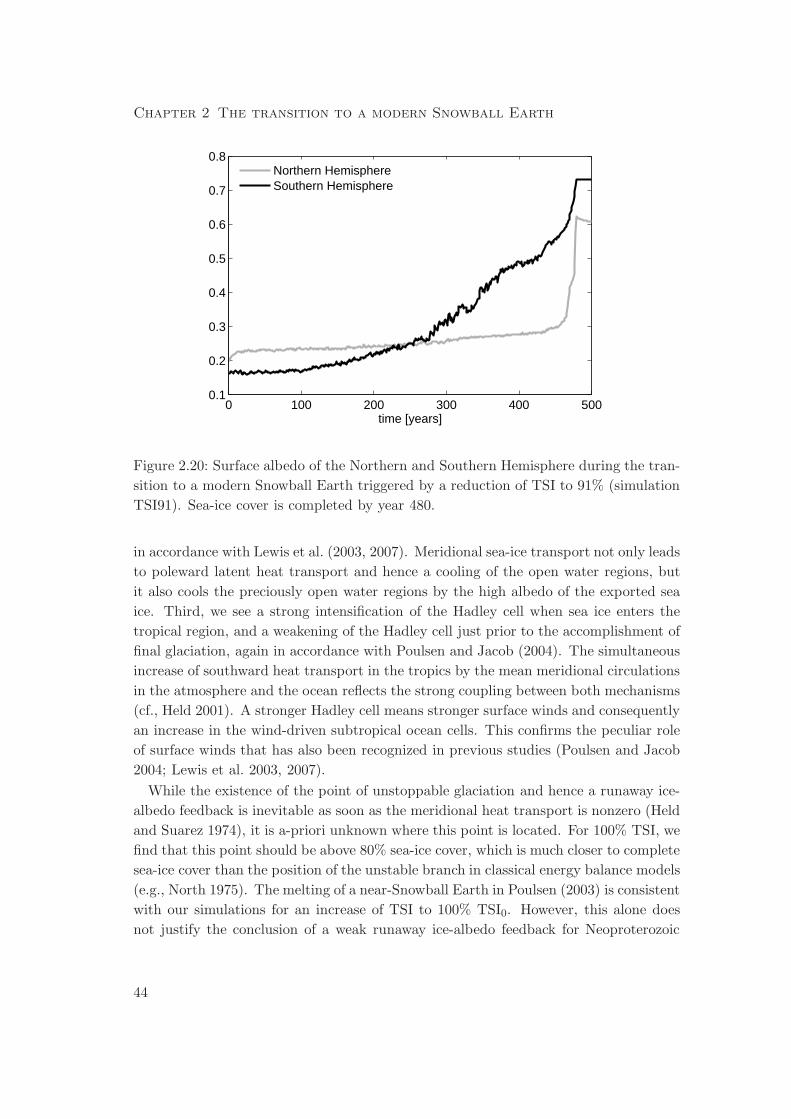
Chapter 2 The transition to a modern Snowball Earth
0 100 200 300 400 5000.1
0.2
0.3
0.4
0.5
0.6
0.7
0.8
time [years]
Northern HemisphereSouthern Hemisphere
Figure 2.20: Surface albedo of the Northern and Southern Hemisphere during the tran-
sition to a modern Snowball Earth triggered by a reduction of TSI to 91% (simulation
TSI91). Sea-ice cover is completed by year 480.
in accordance with Lewis et al. (2003, 2007). Meridional sea-ice transport not only leads
to poleward latent heat transport and hence a cooling of the open water regions, but
it also cools the preciously open water regions by the high albedo of the exported sea
ice. Third, we see a strong intensification of the Hadley cell when sea ice enters the
tropical region, and a weakening of the Hadley cell just prior to the accomplishment of
final glaciation, again in accordance with Poulsen and Jacob (2004). The simultaneous
increase of southward heat transport in the tropics by the mean meridional circulations
in the atmosphere and the ocean reflects the strong coupling between both mechanisms
(cf., Held 2001). A stronger Hadley cell means stronger surface winds and consequently
an increase in the wind-driven subtropical ocean cells. This confirms the peculiar role
of surface winds that has also been recognized in previous studies (Poulsen and Jacob
2004; Lewis et al. 2003, 2007).
While the existence of the point of unstoppable glaciation and hence a runaway ice-
albedo feedback is inevitable as soon as the meridional heat transport is nonzero (Held
and Suarez 1974), it is a-priori unknown where this point is located. For 100% TSI, we
find that this point should be above 80% sea-ice cover, which is much closer to complete
sea-ice cover than the position of the unstable branch in classical energy balance models
(e.g., North 1975). The melting of a near-Snowball Earth in Poulsen (2003) is consistent
with our simulations for an increase of TSI to 100% TSI0. However, this alone does
not justify the conclusion of a weak runaway ice-albedo feedback for Neoproterozoic
44
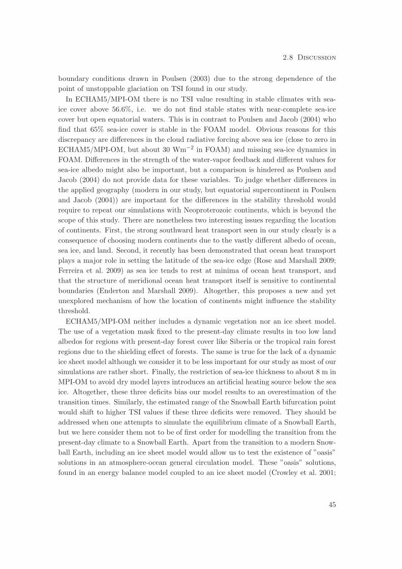
2.8 Discussion
boundary conditions drawn in Poulsen (2003) due to the strong dependence of the
point of unstoppable glaciation on TSI found in our study.
In ECHAM5/MPI-OM there is no TSI value resulting in stable climates with sea-
ice cover above 56.6%, i.e. we do not find stable states with near-complete sea-ice
cover but open equatorial waters. This is in contrast to Poulsen and Jacob (2004) who
find that 65% sea-ice cover is stable in the FOAM model. Obvious reasons for this
discrepancy are differences in the cloud radiative forcing above sea ice (close to zero in
ECHAM5/MPI-OM, but about 30 Wm−2 in FOAM) and missing sea-ice dynamics in
FOAM. Differences in the strength of the water-vapor feedback and different values for
sea-ice albedo might also be important, but a comparison is hindered as Poulsen and
Jacob (2004) do not provide data for these variables. To judge whether differences in
the applied geography (modern in our study, but equatorial supercontinent in Poulsen
and Jacob (2004)) are important for the differences in the stability threshold would
require to repeat our simulations with Neoproterozoic continents, which is beyond the
scope of this study. There are nonetheless two interesting issues regarding the location
of continents. First, the strong southward heat transport seen in our study clearly is a
consequence of choosing modern continents due to the vastly different albedo of ocean,
sea ice, and land. Second, it recently has been demonstrated that ocean heat transport
plays a major role in setting the latitude of the sea-ice edge (Rose and Marshall 2009;
Ferreira et al. 2009) as sea ice tends to rest at minima of ocean heat transport, and
that the structure of meridional ocean heat transport itself is sensitive to continental
boundaries (Enderton and Marshall 2009). Altogether, this proposes a new and yet
unexplored mechanism of how the location of continents might influence the stability
threshold.
ECHAM5/MPI-OM neither includes a dynamic vegetation nor an ice sheet model.
The use of a vegetation mask fixed to the present-day climate results in too low land
albedos for regions with present-day forest cover like Siberia or the tropical rain forest
regions due to the shielding effect of forests. The same is true for the lack of a dynamic
ice sheet model although we consider it to be less important for our study as most of our
simulations are rather short. Finally, the restriction of sea-ice thickness to about 8 m in
MPI-OM to avoid dry model layers introduces an artificial heating source below the sea
ice. Altogether, these three deficits bias our model results to an overestimation of the
transition times. Similarly, the estimated range of the Snowball Earth bifurcation point
would shift to higher TSI values if these three deficits were removed. They should be
addressed when one attempts to simulate the equilibrium climate of a Snowball Earth,
but we here consider them not to be of first order for modelling the transition from the
present-day climate to a Snowball Earth. Apart from the transition to a modern Snow-
ball Earth, including an ice sheet model would allow us to test the existence of ”oasis”
solutions in an atmosphere-ocean general circulation model. These ”oasis” solutions,
found in an energy balance model coupled to an ice sheet model (Crowley et al. 2001;
45
Chapter 2 The transition to a modern Snowball Earth
Peltier et al. 2004, 2007), exhibit tropical land glaciers while tropical oceans remain sea-
ice free and are located in between the present-day like mode and the Snowball Earth
mode in plots of global surface temperature vs. total solar irradiance or longwave CO2
forcing.
We have only modelled the physical climate system comprising atmosphere, ocean,
and sea ice. Atmospheric carbon dioxide levels are fixed in our study. It is certainly
interesting to include the interactions of climate and carbon dioxide in Snowball Earth
simulations. For example, the continental break-up of Rodinia was shown to trigger a
Snowball Earth due to an increase in runoff and due to basaltic traps in the GEOCLIM
model (Donnadieu et al. 2004a; Godderis et al. 2007). Moreover, it has been suggested
that including the Neoproterozoic carbon cycle proposed by Rothman et al. (2003) may
inhibit global glaciations (Peltier et al. 2007) though this is still a matter of debate
(Godderis and Donnadieu 2008; Hoffman et al. 2008; Peltier and Liu 2008). We leave
these issues for future research.
2.9 Conclusions
Based on our simulations with the coupled atmosphere-ocean general circulation model
ECHAM5/MPI-OM to study the transition from the present-day climate to a modern
Snowball Earth, we conclude the following:
1. The Snowball Earth bifurcation point of ECHAM5/MPI-OM is between 91% and
94% of the present-day total solar irradiance (TSI), in agreement with the FOAM
atmosphere ocean general circulation model (Poulsen and Jacob 2004). The tran-
sition time from the present-day climate to a modern Snowball Earth increases
from 14 years for virtually switching off the sun to 480 years for decreasing TSI
to 91% of its present-day value.
2. The Snowball Earth bifurcation point and the transition time found with
ECHAM5/MPI-OM are well reproduced with a zero-dimensional energy balance
model of the mean ocean potential temperature.
3. The asymmetric distribution of continents between the Northern and Southern
Hemispheres causes strong heat transports toward the more water-covered South-
ern Hemisphere as sea ice spreads towards the equator. The southern Hadley cell
and the wind-driven subtropical ocean cells strengthen by a factor of 4 as sea ice
approaches the equator.
4. For 100% TSI the point of unstoppable glaciation is much closer to complete sea-
ice cover than in classical energy balance models. Stable states have no greater
than 56.6% sea-ice cover implying that ECHAM5/MPI-OM does not exhibit sta-
ble states with near-complete sea-ice cover but open equatorial waters.
46
Chapter 3
Initiation of a Marinoan Snowball Earth in
a state-of-the-art atmosphere-ocean
general circulation model
We use the state-of-the-art atmosphere-ocean general circulation model ECHAM5/MPI-
OM to revisit the initiation of a Snowball Earth for Marinoan surface boundary condi-
tions (635 million years before present). The comparison with a pre-industrial control
climate shows that the change of surface boundary conditions from present-day to Mari-
noan, including a shift of continents to low latitudes, induces a global-mean cooling of
4.6 K. Two thirds of this cooling can be attributed to increased planetary albedo, the
remaining one third to increased effective emissivity, i.e. a weaker greenhouse effect.
The Marinoan Snowball Earth bifurcation point for pre-industrial atmospheric carbon
dioxide is between 95.5 and 96% of the present-day total solar irradiance (TSI), im-
plying that Snowball Earth initiation is much easier for Marinoan than present-day
surface boundary conditions. A Snowball Earth for TSI set to its Marinoan value
(94% of the present-day TSI), is prevented by quadrupling carbon dioxide with re-
spect to its pre-industrial level. A zero-dimensional energy balance model successfully
predicts the Snowball Earth bifurcation point by only knowing the equilibrium global-
mean ocean potential temperature for the present-day value of TSI. Sea-ice cover above
55% is unstable, akin to what was found for present-day surface boundary conditions.
ECHAM5/MPI-OM hence does not exhibit states with near-complete sea-ice cover but
open equatorial waters. In summary, Snowball Earth initiation in a state-of-the-art cou-
pled climate model is possible for Marinoan surface boundary conditions and Marinoan
TSI by reducing atmospheric carbon dioxide to its pre-industrial level. This contradicts
previous conclusions that Snowball Earth initiation would require ”extreme” forcings.
3.1 Introduction
The apparent existence of low-latitude land glaciers at sea level during at least two
episodes of the Neoproterozoic era, the Sturtian (∼ 710 million years before present,
47
Chapter 3 Initiation of a Marinoan Snowball Earth
Ma) and the Marinoan(∼ 635 Ma) (Evans 2000; Trindade and Macouin 2007; Mac-
donald et al. 2010), has led to the proposal that these glaciations must have been
accompanied by completely frozen oceans. This so-called ”Snowball Earth” hypoth-
esis (Kirschvink 1992; Hoffman et al. 1998) has not only attracted the attention of
geologists, but also of climate modellers, who have tested if the Snowball Earth hy-
pothesis is compatible with climate physics. In this study, we use the state-of-the-art
atmosphere-ocean general circulation model ECHAM5/MPI-OM to revisit the initia-
tion of a Snowball Earth for Marinoan surface boundary conditions, a main feature
of the latter being the preponderance of continents in low latitudes. In particular, we
investigate the Snowball Earth bifurcation point and the maximum stable sea-ice cover.
We are by far not the first to confront the Snowball Earth hypothesis with climate
models. Indeed, the Snowball Earth hypothesis itself relies on a runaway ice-albedo
feedback first reported in energy balance models (e.g., Budyko 1969; Sellers 1969). Af-
ter the initial perception that the Snowball Earth hypothesis is, in principle, compatible
with climate physics, the last decade has seen the full hierarchy of climate models being
applied to Snowball Earth initiation. While we do not know of any climate model that
excludes Snowball Earth solutions categorically, various climate modelling studies con-
cluded that completely frozen oceans require ”extreme” forcings (Chandler and Sohl
2000; Poulsen et al. 2001; Poulsen 2003; Poulsen and Jacob 2004) that might be consid-
ered unrealistic for the Neoproterozoic. At the same time, Hyde et al. (2000) and Peltier
et al. (2004), using an energy balance model with interactive ice sheets, found so-called
”Slushball Earth” or ”oasis” solutions that are characterized by tropical land glacia-
tion but open equatorial water. Despite severe limitations of their model, including the
disregard of atmosphere and ocean dynamics, these solutions have been supported by
an atmospheric general circulation model coupled to a slab ocean and prescribed full
continental glaciation (Hyde et al. 2000; Baum and Crowley 2001). Moreover, Chandler
and Sohl (2000) and Micheels and Montenari (2008) found, also using atmospheric gen-
eral circulation models coupled to slab oceans, solutions with equatorial land masses
below freezing in conjunction with almost but not completely frozen oceans. As a re-
sult, the apparent difficulties in freezing the entire ocean combined with the possibility
that equatorial land glaciers might not require completely frozen oceans evoked the
impression that the Snowball Earth hypothesis was implausible from the perspective
of climate modelling, and attention shifted to the Slushball Earth hypothesis (Lubick
2002; Kaufman 2007; Kerr 2010).
We here study the initiation of a Marinoan Snowball Earth in the state-of-the art
atmosphere-ocean general circulation model ECHAM5/MPI-OM. This model incorpo-
rates physics found to be essential for Snowball Earth initiation but neglected in models
supporting the Slushball Earth hypothesis, including ocean dynamics (Poulsen et al.
2001; Poulsen and Jacob 2004), sea-ice dynamics (Lewis et al. 2003, 2007) and clouds
(Poulsen and Jacob 2004). By comparing the simulations to a previous study of two of
48
3.2 Model and simulation setup
us with this model for present-day surface boundary conditions (Voigt and Marotzke
2009), we also can reevaluate if low-latitude continents favor Snowball Earth initia-
tion as suggested by Kirschvink (1992), something that was rebutted by Poulsen et al.
(2002).
This study addresses two issues. First, we investigate the climatic effect of changing
surface boundary conditions from present-day to Marinoan. To this end, we generate a
Marinoan control climate for present-day total solar irradiance (TSI) and pre-industrial
greenhouse gas concentrations by integrating the model to equilibrium (∼ 3500 years)
for Marinoan surface boundary conditions. We compare the Marinoan control climate
to the pre-industrial control climate by means of a one-dimensional energy balance
model. This allows us to identify and quantify the mechanisms responsible for the
surface temperature change induced by the change of surface boundary conditions.
Second, we estimate the Snowball Earth bifurcation point and the maximum stable
sea-ice cover of the model for Marinoan surface boundary conditions. For this, we
start the model from the Marinoan control climate and abruptly decrease TSI, in some
cases combined with an simultaneous increase of carbon dioxide. This is the same
experimental strategy as in Voigt and Marotzke (2009).
The paper is organised as follows. Section 2 describes the climate model, the Mari-
noan surface boundary conditions, and the setup of the ECHAM5/MPI-OM simula-
tions, including the spinup of the Marinoan control climate. Section 3 analyzes the
Marinoan control climate and compares it to a pre-industrial control simulation by
means of a one-dimensional energy balance model of zonal mean surface temperature.
Section 4 investigates the Snowball Earth bifurcation point and maximum stable sea-ice
cover. A zero-dimensional energy balance model of the diagnosed global-mean ocean
potential temperature is used to predict the Snowball Earth bifurcation point in Sec-
tion 5. Section 6 points at an imbalance of the global-mean top of atmosphere and
surface energy fluxes. Section 7 gives a general discussion of the results, Sect. 8 follows
with conclusions.
3.2 Model and simulation setup
3.2.1 Model setup
We apply the state-of-the-art atmosphere-ocean general circulation model
ECHAM5/MPI-OM. This is the same model that was used to study the transition to
a modern Snowball Earth (Voigt and Marotzke 2009), apart from technical changes to
adapt the model to the new supercomputer of the German Climate Computing Center
(DKRZ). ECHAM5/MPI-OM ranks among the world’s top climate models and has
been used for a variety of applications, ranging from climate projections for the Inter-
governmental Panel on Climate Change (Solomon et al. 2007), including sea-level rise
49
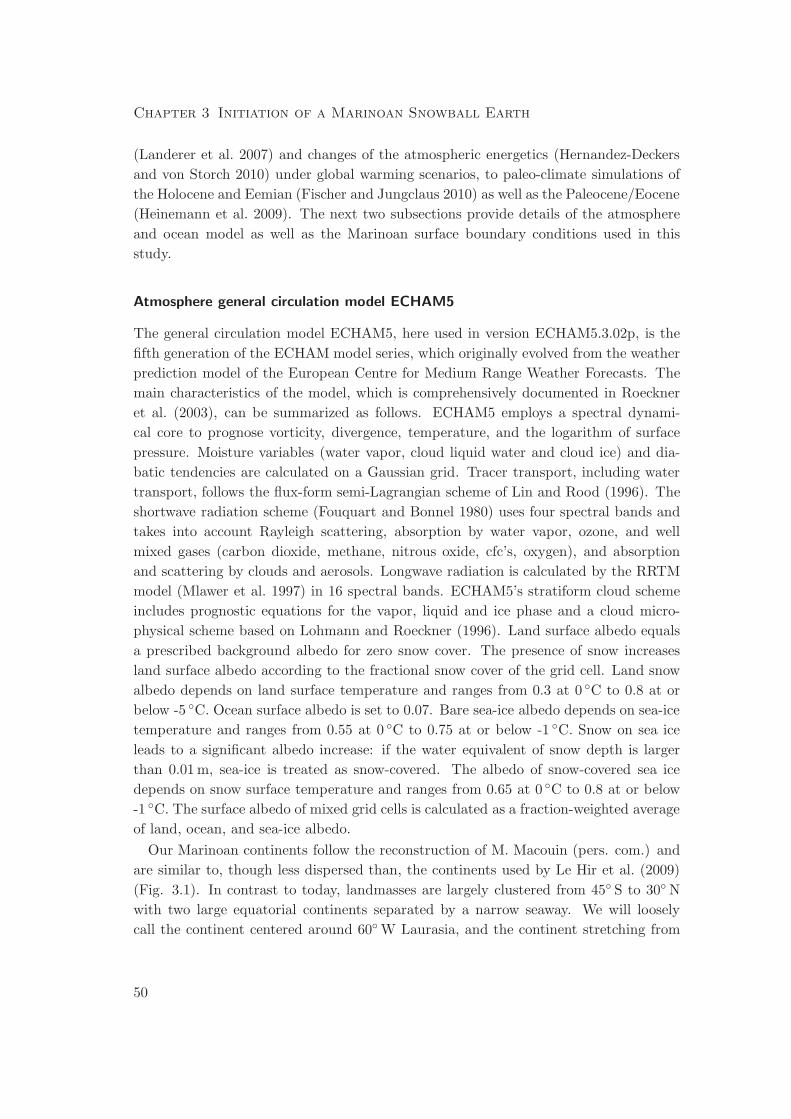
Chapter 3 Initiation of a Marinoan Snowball Earth
(Landerer et al. 2007) and changes of the atmospheric energetics (Hernandez-Deckers
and von Storch 2010) under global warming scenarios, to paleo-climate simulations of
the Holocene and Eemian (Fischer and Jungclaus 2010) as well as the Paleocene/Eocene
(Heinemann et al. 2009). The next two subsections provide details of the atmosphere
and ocean model as well as the Marinoan surface boundary conditions used in this
study.
Atmosphere general circulation model ECHAM5
The general circulation model ECHAM5, here used in version ECHAM5.3.02p, is the
fifth generation of the ECHAM model series, which originally evolved from the weather
prediction model of the European Centre for Medium Range Weather Forecasts. The
main characteristics of the model, which is comprehensively documented in Roeckner
et al. (2003), can be summarized as follows. ECHAM5 employs a spectral dynami-
cal core to prognose vorticity, divergence, temperature, and the logarithm of surface
pressure. Moisture variables (water vapor, cloud liquid water and cloud ice) and dia-
batic tendencies are calculated on a Gaussian grid. Tracer transport, including water
transport, follows the flux-form semi-Lagrangian scheme of Lin and Rood (1996). The
shortwave radiation scheme (Fouquart and Bonnel 1980) uses four spectral bands and
takes into account Rayleigh scattering, absorption by water vapor, ozone, and well
mixed gases (carbon dioxide, methane, nitrous oxide, cfc’s, oxygen), and absorption
and scattering by clouds and aerosols. Longwave radiation is calculated by the RRTM
model (Mlawer et al. 1997) in 16 spectral bands. ECHAM5’s stratiform cloud scheme
includes prognostic equations for the vapor, liquid and ice phase and a cloud micro-
physical scheme based on Lohmann and Roeckner (1996). Land surface albedo equals
a prescribed background albedo for zero snow cover. The presence of snow increases
land surface albedo according to the fractional snow cover of the grid cell. Land snow
albedo depends on land surface temperature and ranges from 0.3 at 0 ◦C to 0.8 at or
below -5 ◦C. Ocean surface albedo is set to 0.07. Bare sea-ice albedo depends on sea-ice
temperature and ranges from 0.55 at 0 ◦C to 0.75 at or below -1 ◦C. Snow on sea ice
leads to a significant albedo increase: if the water equivalent of snow depth is larger
than 0.01 m, sea-ice is treated as snow-covered. The albedo of snow-covered sea ice
depends on snow surface temperature and ranges from 0.65 at 0 ◦C to 0.8 at or below
-1 ◦C. The surface albedo of mixed grid cells is calculated as a fraction-weighted average
of land, ocean, and sea-ice albedo.
Our Marinoan continents follow the reconstruction of M. Macouin (pers. com.) and
are similar to, though less dispersed than, the continents used by Le Hir et al. (2009)
(Fig. 3.1). In contrast to today, landmasses are largely clustered from 45◦ S to 30◦ N
with two large equatorial continents separated by a narrow seaway. We will loosely
call the continent centered around 60◦ W Laurasia, and the continent stretching from
50
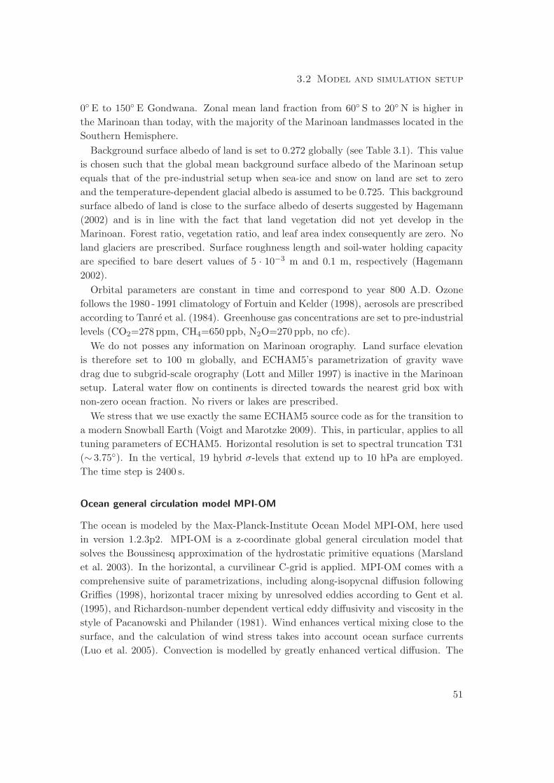
3.2 Model and simulation setup
0◦ E to 150◦ E Gondwana. Zonal mean land fraction from 60◦ S to 20◦ N is higher in
the Marinoan than today, with the majority of the Marinoan landmasses located in the
Southern Hemisphere.
Background surface albedo of land is set to 0.272 globally (see Table 3.1). This value
is chosen such that the global mean background surface albedo of the Marinoan setup
equals that of the pre-industrial setup when sea-ice and snow on land are set to zero
and the temperature-dependent glacial albedo is assumed to be 0.725. This background
surface albedo of land is close to the surface albedo of deserts suggested by Hagemann
(2002) and is in line with the fact that land vegetation did not yet develop in the
Marinoan. Forest ratio, vegetation ratio, and leaf area index consequently are zero. No
land glaciers are prescribed. Surface roughness length and soil-water holding capacity
are specified to bare desert values of 5 · 10−3 m and 0.1 m, respectively (Hagemann
2002).
Orbital parameters are constant in time and correspond to year 800 A.D. Ozone
follows the 1980 - 1991 climatology of Fortuin and Kelder (1998), aerosols are prescribed
according to Tanre et al. (1984). Greenhouse gas concentrations are set to pre-industrial
levels (CO2=278 ppm, CH4=650 ppb, N2O=270 ppb, no cfc).
We do not posses any information on Marinoan orography. Land surface elevation
is therefore set to 100 m globally, and ECHAM5’s parametrization of gravity wave
drag due to subgrid-scale orography (Lott and Miller 1997) is inactive in the Marinoan
setup. Lateral water flow on continents is directed towards the nearest grid box with
non-zero ocean fraction. No rivers or lakes are prescribed.
We stress that we use exactly the same ECHAM5 source code as for the transition to
a modern Snowball Earth (Voigt and Marotzke 2009). This, in particular, applies to all
tuning parameters of ECHAM5. Horizontal resolution is set to spectral truncation T31
(∼ 3.75◦). In the vertical, 19 hybrid σ-levels that extend up to 10 hPa are employed.
The time step is 2400 s.
Ocean general circulation model MPI-OM
The ocean is modeled by the Max-Planck-Institute Ocean Model MPI-OM, here used
in version 1.2.3p2. MPI-OM is a z-coordinate global general circulation model that
solves the Boussinesq approximation of the hydrostatic primitive equations (Marsland
et al. 2003). In the horizontal, a curvilinear C-grid is applied. MPI-OM comes with a
comprehensive suite of parametrizations, including along-isopycnal diffusion following
Griffies (1998), horizontal tracer mixing by unresolved eddies according to Gent et al.
(1995), and Richardson-number dependent vertical eddy diffusivity and viscosity in the
style of Pacanowski and Philander (1981). Wind enhances vertical mixing close to the
surface, and the calculation of wind stress takes into account ocean surface currents
(Luo et al. 2005). Convection is modelled by greatly enhanced vertical diffusion. The
51
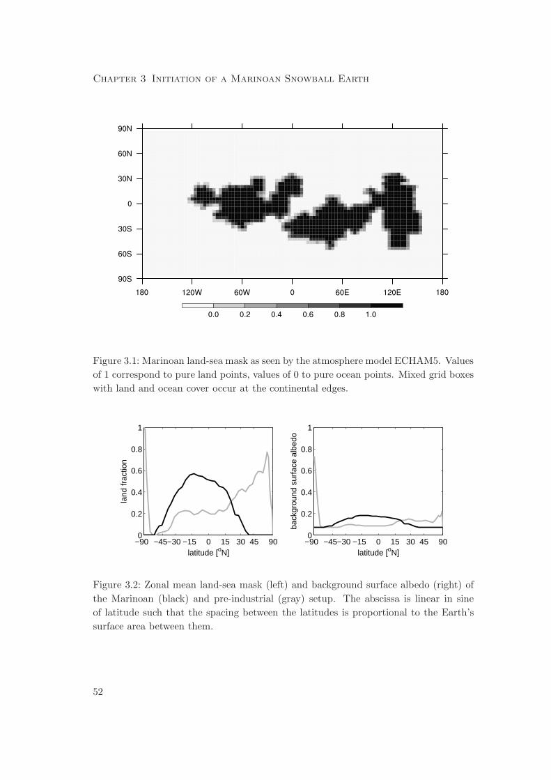
Chapter 3 Initiation of a Marinoan Snowball Earth
Figure 3.1: Marinoan land-sea mask as seen by the atmosphere model ECHAM5. Values
of 1 correspond to pure land points, values of 0 to pure ocean points. Mixed grid boxes
with land and ocean cover occur at the continental edges.
−90 −45−30 −15 0 15 30 45 900
0.2
0.4
0.6
0.8
1
land
frac
tion
latitude [oN]−90 −45−30 −15 0 15 30 45 900
0.2
0.4
0.6
0.8
1
back
grou
nd s
urfa
ce a
lbed
o
latitude [oN]
Figure 3.2: Zonal mean land-sea mask (left) and background surface albedo (right) of
the Marinoan (black) and pre-industrial (gray) setup. The abscissa is linear in sine
of latitude such that the spacing between the latitudes is proportional to the Earth’s
surface area between them.
52
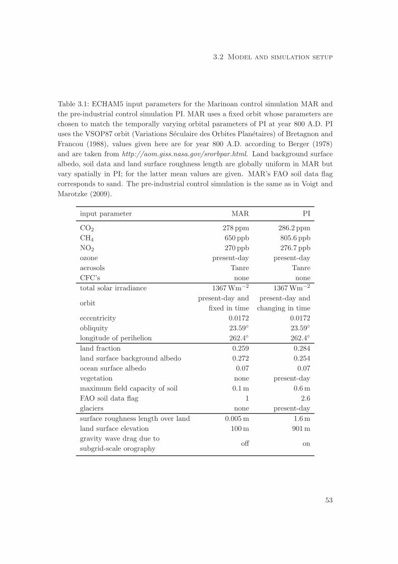
3.2 Model and simulation setup
Table 3.1: ECHAM5 input parameters for the Marinoan control simulation MAR and
the pre-industrial control simulation PI. MAR uses a fixed orbit whose parameters are
chosen to match the temporally varying orbital parameters of PI at year 800 A.D. PI
uses the VSOP87 orbit (Variations Seculaire des Orbites Planetaires) of Bretagnon and
Francou (1988), values given here are for year 800 A.D. according to Berger (1978)
and are taken from http://aom.giss.nasa.gov/srorbpar.html. Land background surface
albedo, soil data and land surface roughness length are globally uniform in MAR but
vary spatially in PI; for the latter mean values are given. MAR’s FAO soil data flag
corresponds to sand. The pre-industrial control simulation is the same as in Voigt and
Marotzke (2009).
input parameter MAR PI
CO2 278 ppm 286.2 ppm
CH4 650 ppb 805.6 ppb
NO2 270 ppb 276.7 ppb
ozone present-day present-day
aerosols Tanre Tanre
CFC’s none none
total solar irradiance 1367 Wm−2 1367 Wm−2
orbitpresent-day and present-day and
fixed in time changing in time
eccentricity 0.0172 0.0172
obliquity 23.59◦ 23.59◦
longitude of perihelion 262.4◦ 262.4◦
land fraction 0.259 0.284
land surface background albedo 0.272 0.254
ocean surface albedo 0.07 0.07
vegetation none present-day
maximum field capacity of soil 0.1 m 0.6 m
FAO soil data flag 1 2.6
glaciers none present-day
surface roughness length over land 0.005 m 1.6 m
land surface elevation 100 m 901 m
gravity wave drag due tooff on
subgrid-scale orography
53
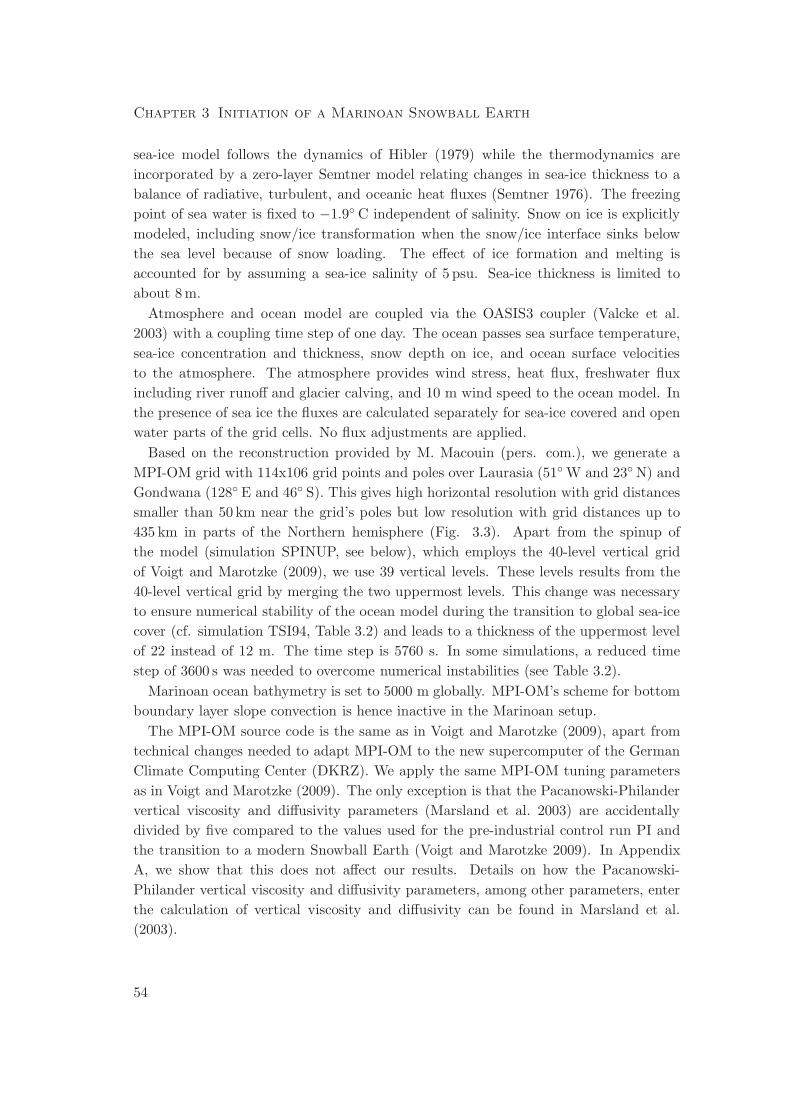
Chapter 3 Initiation of a Marinoan Snowball Earth
sea-ice model follows the dynamics of Hibler (1979) while the thermodynamics are
incorporated by a zero-layer Semtner model relating changes in sea-ice thickness to a
balance of radiative, turbulent, and oceanic heat fluxes (Semtner 1976). The freezing
point of sea water is fixed to −1.9◦ C independent of salinity. Snow on ice is explicitly
modeled, including snow/ice transformation when the snow/ice interface sinks below
the sea level because of snow loading. The effect of ice formation and melting is
accounted for by assuming a sea-ice salinity of 5 psu. Sea-ice thickness is limited to
about 8 m.
Atmosphere and ocean model are coupled via the OASIS3 coupler (Valcke et al.
2003) with a coupling time step of one day. The ocean passes sea surface temperature,
sea-ice concentration and thickness, snow depth on ice, and ocean surface velocities
to the atmosphere. The atmosphere provides wind stress, heat flux, freshwater flux
including river runoff and glacier calving, and 10 m wind speed to the ocean model. In
the presence of sea ice the fluxes are calculated separately for sea-ice covered and open
water parts of the grid cells. No flux adjustments are applied.
Based on the reconstruction provided by M. Macouin (pers. com.), we generate a
MPI-OM grid with 114x106 grid points and poles over Laurasia (51◦ W and 23◦ N) and
Gondwana (128◦ E and 46◦ S). This gives high horizontal resolution with grid distances
smaller than 50 km near the grid’s poles but low resolution with grid distances up to
435 km in parts of the Northern hemisphere (Fig. 3.3). Apart from the spinup of
the model (simulation SPINUP, see below), which employs the 40-level vertical grid
of Voigt and Marotzke (2009), we use 39 vertical levels. These levels results from the
40-level vertical grid by merging the two uppermost levels. This change was necessary
to ensure numerical stability of the ocean model during the transition to global sea-ice
cover (cf. simulation TSI94, Table 3.2) and leads to a thickness of the uppermost level
of 22 instead of 12 m. The time step is 5760 s. In some simulations, a reduced time
step of 3600 s was needed to overcome numerical instabilities (see Table 3.2).
Marinoan ocean bathymetry is set to 5000 m globally. MPI-OM’s scheme for bottom
boundary layer slope convection is hence inactive in the Marinoan setup.
The MPI-OM source code is the same as in Voigt and Marotzke (2009), apart from
technical changes needed to adapt MPI-OM to the new supercomputer of the German
Climate Computing Center (DKRZ). We apply the same MPI-OM tuning parameters
as in Voigt and Marotzke (2009). The only exception is that the Pacanowski-Philander
vertical viscosity and diffusivity parameters (Marsland et al. 2003) are accidentally
divided by five compared to the values used for the pre-industrial control run PI and
the transition to a modern Snowball Earth (Voigt and Marotzke 2009). In Appendix
A, we show that this does not affect our results. Details on how the Pacanowski-
Philander vertical viscosity and diffusivity parameters, among other parameters, enter
the calculation of vertical viscosity and diffusivity can be found in Marsland et al.
(2003).
54
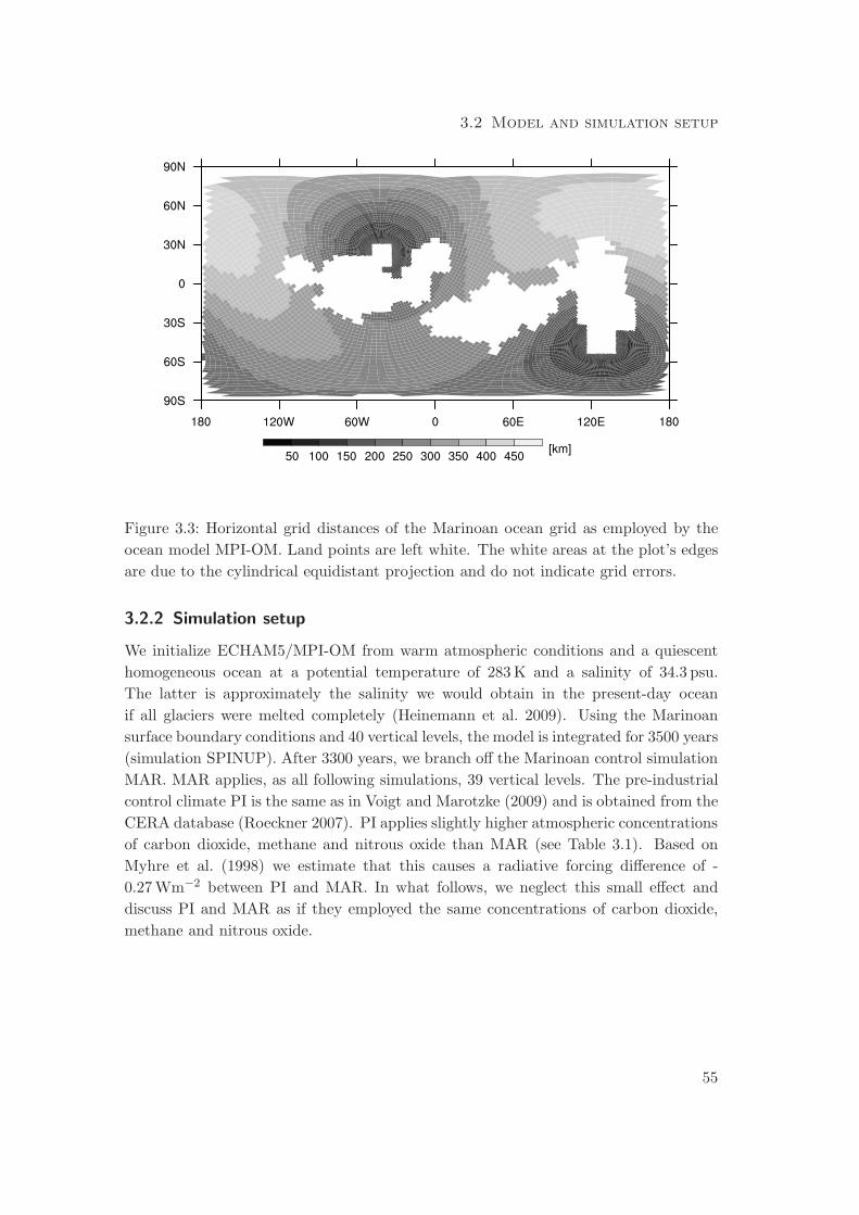
3.2 Model and simulation setup
Figure 3.3: Horizontal grid distances of the Marinoan ocean grid as employed by the
ocean model MPI-OM. Land points are left white. The white areas at the plot’s edges
are due to the cylindrical equidistant projection and do not indicate grid errors.
3.2.2 Simulation setup
We initialize ECHAM5/MPI-OM from warm atmospheric conditions and a quiescent
homogeneous ocean at a potential temperature of 283 K and a salinity of 34.3 psu.
The latter is approximately the salinity we would obtain in the present-day ocean
if all glaciers were melted completely (Heinemann et al. 2009). Using the Marinoan
surface boundary conditions and 40 vertical levels, the model is integrated for 3500 years
(simulation SPINUP). After 3300 years, we branch off the Marinoan control simulation
MAR. MAR applies, as all following simulations, 39 vertical levels. The pre-industrial
control climate PI is the same as in Voigt and Marotzke (2009) and is obtained from the
CERA database (Roeckner 2007). PI applies slightly higher atmospheric concentrations
of carbon dioxide, methane and nitrous oxide than MAR (see Table 3.1). Based on
Myhre et al. (1998) we estimate that this causes a radiative forcing difference of -
0.27 Wm−2 between PI and MAR. In what follows, we neglect this small effect and
discuss PI and MAR as if they employed the same concentrations of carbon dioxide,
methane and nitrous oxide.
55
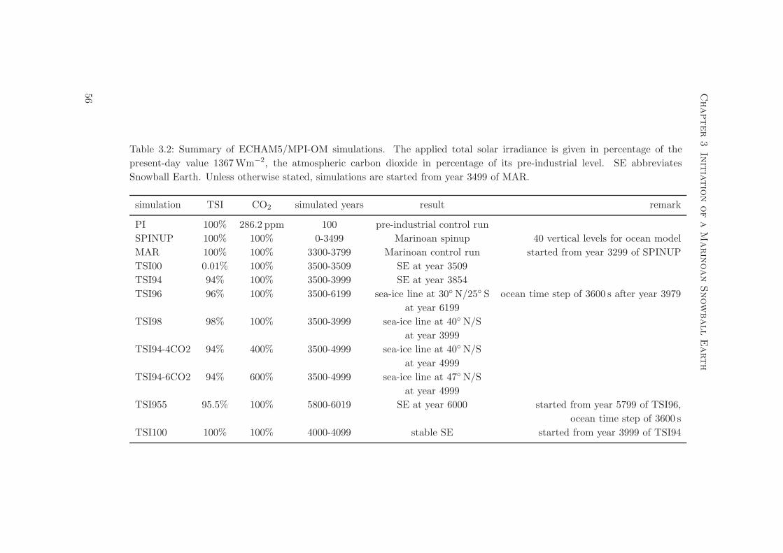
Chapter
3In
itia
tio
nof
aM
arin
oan
Snow
ball
Earth
Table 3.2: Summary of ECHAM5/MPI-OM simulations. The applied total solar irradiance is given in percentage of the
present-day value 1367 Wm−2, the atmospheric carbon dioxide in percentage of its pre-industrial level. SE abbreviates
Snowball Earth. Unless otherwise stated, simulations are started from year 3499 of MAR.
simulation TSI CO2 simulated years result remark
PI 100% 286.2 ppm 100 pre-industrial control run
SPINUP 100% 100% 0-3499 Marinoan spinup 40 vertical levels for ocean model
MAR 100% 100% 3300-3799 Marinoan control run started from year 3299 of SPINUP
TSI00 0.01% 100% 3500-3509 SE at year 3509
TSI94 94% 100% 3500-3999 SE at year 3854
TSI96 96% 100% 3500-6199 sea-ice line at 30◦ N/25◦ S ocean time step of 3600 s after year 3979
at year 6199
TSI98 98% 100% 3500-3999 sea-ice line at 40◦ N/S
at year 3999
TSI94-4CO2 94% 400% 3500-4999 sea-ice line at 40◦ N/S
at year 4999
TSI94-6CO2 94% 600% 3500-4999 sea-ice line at 47◦ N/S
at year 4999
TSI955 95.5% 100% 5800-6019 SE at year 6000 started from year 5799 of TSI96,
ocean time step of 3600 s
TSI100 100% 100% 4000-4099 stable SE started from year 3999 of TSI94
56
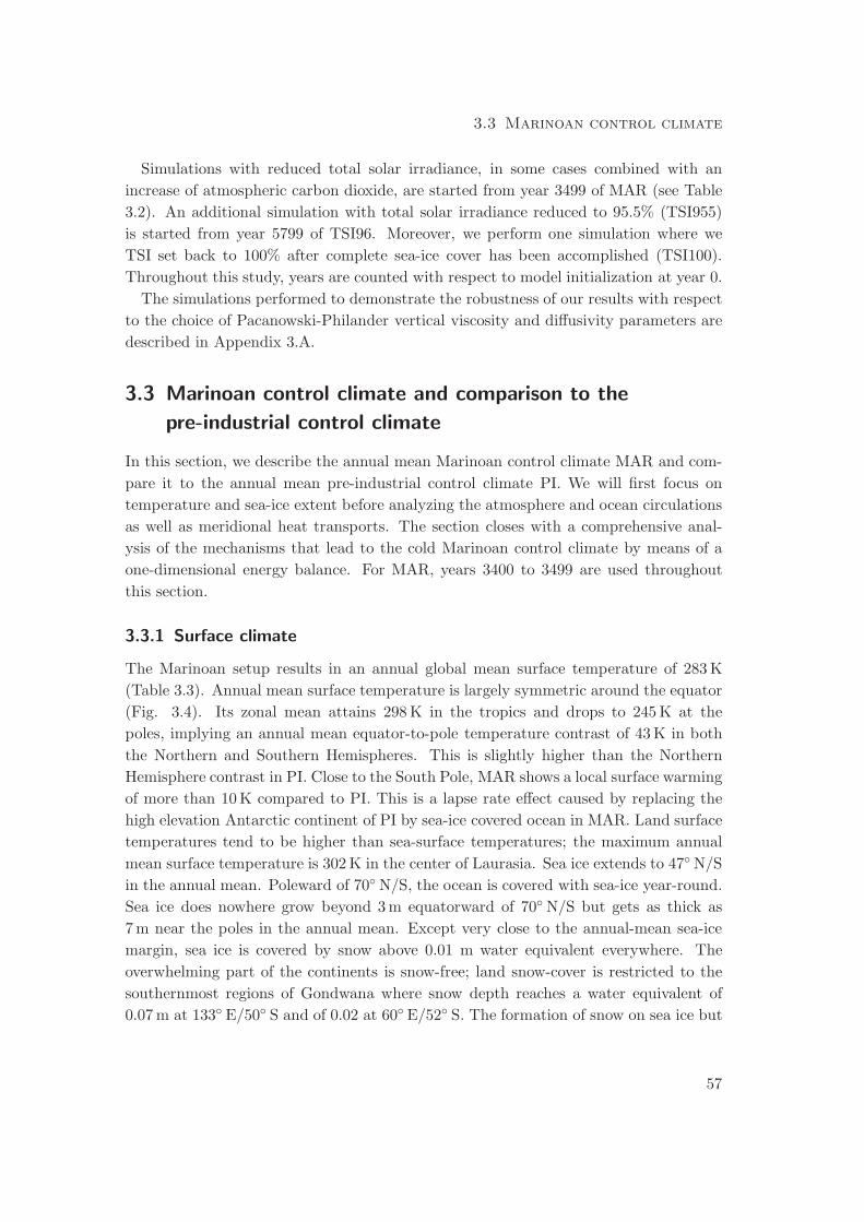
3.3 Marinoan control climate
Simulations with reduced total solar irradiance, in some cases combined with an
increase of atmospheric carbon dioxide, are started from year 3499 of MAR (see Table
3.2). An additional simulation with total solar irradiance reduced to 95.5% (TSI955)
is started from year 5799 of TSI96. Moreover, we perform one simulation where we
TSI set back to 100% after complete sea-ice cover has been accomplished (TSI100).
Throughout this study, years are counted with respect to model initialization at year 0.
The simulations performed to demonstrate the robustness of our results with respect
to the choice of Pacanowski-Philander vertical viscosity and diffusivity parameters are
described in Appendix 3.A.
3.3 Marinoan control climate and comparison to the
pre-industrial control climate
In this section, we describe the annual mean Marinoan control climate MAR and com-
pare it to the annual mean pre-industrial control climate PI. We will first focus on
temperature and sea-ice extent before analyzing the atmosphere and ocean circulations
as well as meridional heat transports. The section closes with a comprehensive anal-
ysis of the mechanisms that lead to the cold Marinoan control climate by means of a
one-dimensional energy balance. For MAR, years 3400 to 3499 are used throughout
this section.
3.3.1 Surface climate
The Marinoan setup results in an annual global mean surface temperature of 283 K
(Table 3.3). Annual mean surface temperature is largely symmetric around the equator
(Fig. 3.4). Its zonal mean attains 298 K in the tropics and drops to 245 K at the
poles, implying an annual mean equator-to-pole temperature contrast of 43 K in both
the Northern and Southern Hemispheres. This is slightly higher than the Northern
Hemisphere contrast in PI. Close to the South Pole, MAR shows a local surface warming
of more than 10 K compared to PI. This is a lapse rate effect caused by replacing the
high elevation Antarctic continent of PI by sea-ice covered ocean in MAR. Land surface
temperatures tend to be higher than sea-surface temperatures; the maximum annual
mean surface temperature is 302 K in the center of Laurasia. Sea ice extends to 47◦ N/S
in the annual mean. Poleward of 70◦ N/S, the ocean is covered with sea-ice year-round.
Sea ice does nowhere grow beyond 3 m equatorward of 70◦ N/S but gets as thick as
7 m near the poles in the annual mean. Except very close to the annual-mean sea-ice
margin, sea ice is covered by snow above 0.01 m water equivalent everywhere. The
overwhelming part of the continents is snow-free; land snow-cover is restricted to the
southernmost regions of Gondwana where snow depth reaches a water equivalent of
0.07 m at 133◦ E/50◦ S and of 0.02 at 60◦ E/52◦ S. The formation of snow on sea ice but
57
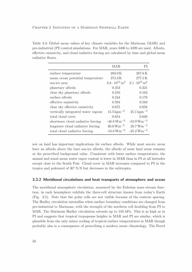
Chapter 3 Initiation of a Marinoan Snowball Earth
Table 3.3: Global mean values of key climate variables for the Marinoan (MAR) and
pre-industrial (PI) control simulations. For MAR, years 3400 to 3499 are used. Albedo,
effective emissivity, and cloud radiative forcing are calculated by time and global mean
radiative fluxes.
MAR PI
surface temperature 283.0 K 287.6 K
mean ocean potential temperature 274.3 K 277.5 K
sea-ice area 8.6 · 1013 m2 2.1 ·1013 m2
planetary albedo 0.353 0.321
clear sky planetary albedo 0.210 0.163
surface albedo 0.244 0.170
effective emissivity 0.594 0.583
clear sky effective emissivity 0.675 0.656
vertically integrated water vapour 15.5 kgm−2 25.1 kgm−2
total cloud cover 0.654 0.620
shortwave cloud radiative forcing -48.8 Wm−2 -53.9 Wm−2
longwave cloud radiative forcing 30.0 Wm−2 28.7 Wm−2
total cloud radiative forcing -18.8 Wm−2 -25.2 Wm−2
not on land has important implications for surface albedo. While most sea-ice areas
have an albedo above the bare sea-ice albedo, the albedo of most land areas remains
at the prescribed background value. Consistent with lower surface temperatures, the
annual and zonal mean water vapor content is lower in MAR than in PI at all latitudes
except close to the South Pole. Cloud cover in MAR increases compared to PI in the
tropics and poleward of 30◦ N/S but decreases in the subtropics.
3.3.2 Meridional circulations and heat transports of atmosphere and ocean
The meridional atmospheric circulation, measured by the Eulerian mass stream func-
tion, in each hemisphere exhibits the three-cell structure known from today’s Earth
(Fig. 3.5). Note that the polar cells are not visible because of the contour spacing.
The Hadley circulation intensifies when surface boundary conditions are changed from
pre-industrial to Marinoan, with the strength of the northern cell doubling from PI to
MAR. The Marinoan Hadley circulation extends up to 150 hPa. This is as high as in
PI and suggests that tropical tropopause heights in MAR and PI are similar, which is
plausible from the only minor cooling of tropical surface temperatures in MAR though
probably also is a consequence of prescribing a modern ozone climatology. The Ferrel
58
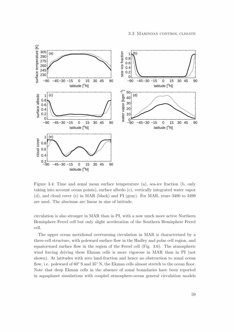
3.3 Marinoan control climate
−90 −45−30 −15 0 15 30 45 90
230245260275290305
latitude [oN]
surf
ace
tem
pera
ture
[K]
(a)
−90 −45−30 −15 0 15 30 45 900
0.20.40.60.8
1
latitude [oN]
sea−
ice
frac
tion (b)
−90 −45−30 −15 0 15 30 45 900
0.20.40.60.8
1
latitude [oN]
surf
ace
albe
do (c)
−90 −45−30 −15 0 15 30 45 900
10
20
30
40
50
latitude [oN]w
ater
vap
or [k
gm−
2 ]
(d)
−90 −45−30 −15 0 15 30 45 900.2
0.4
0.6
0.8
1
latitude [oN]
clou
d co
ver (e)
Figure 3.4: Time and zonal mean surface temperature (a), sea-ice fraction (b, only
taking into account ocean points), surface albedo (c), vertically integrated water vapor
(d), and cloud cover (e) in MAR (black) and PI (gray). For MAR, years 3400 to 3499
are used. The abscissae are linear in sine of latitude.
circulation is also stronger in MAR than in PI, with a now much more active Northern
Hemisphere Ferrel cell but only slight acceleration of the Southern Hemisphere Ferrel
cell.
The upper ocean meridional overturning circulation in MAR is characterized by a
three-cell structure, with poleward surface flow in the Hadley and polar cell region, and
equatorward surface flow in the region of the Ferrel cell (Fig. 3.6). The atmospheric
wind forcing driving these Ekman cells is more vigorous in MAR than in PI (not
shown). At latitudes with zero land-fraction and hence no obstruction to zonal ocean
flow, i.e. poleward of 60◦ S and 35◦ N, the Ekman cells almost stretch to the ocean floor.
Note that deep Ekman cells in the absence of zonal boundaries have been reported
in aquaplanet simulations with coupled atmosphere-ocean general circulation models
59
Chapter 3 Initiation of a Marinoan Snowball Earth
(Smith et al. 2006; Marshall et al. 2007). They are a consequence of vanishing zonal
pressure gradient and largely zonally-symmetric flow such that the return flow to the
wind-generated meridional surface flow must be balanced by zonal momentum diffusion
in the ocean interior and bottom friction at the ocean floor (Smith et al. 2006). The
mid and deep ocean in MAR does not show the present-day structure of clockwise
interhemispheric flow between 1 and 3 km and counterclockwise interhemispheric flow
below. Instead, MAR exhibits a counterclockwise interhemispheric circulation below
500 m with downward motion between 30 and 50◦ S and upward motion within the
deep Northern Hemisphere Ekman cell centered around 45◦ N. There is no significant
clockwise flow in the deep ocean, i.e. no Marinoan correspondent to today’s Antarctic
Bottom Water cell. In MAR, vigorous circumpolar currents that reach 750 Sv in the
Northern and 250 Sv in the Southern hemisphere develop (Fig. 3.7). They are in
geostrophic balance with large meridional sea-level gradients around the sea-ice margin
at 47◦ N/S. These gradients are consistent with strong meridional gradients of ocean
potential temperature at these latitudes, a consequence of cooling the water column
to close to the freezing point below sea ice. Subtropical ocean gyres with magnitudes
larger than 50 Sv and western boundary intensification develop in MAR, similar to PI.
Moreover, MAR exhibits weak tropical gyres, again akin to PI.
Compared to PI, total advective atmospheric heat transport in MAR is larger in
the tropics but tends to be smaller in the extratropics (Fig. 3.8). The intensification
of the mean meridional circulation is associated with an increase of its contribution
to the atmospheric heat transport at almost all latitudes, which explains the stronger
heat transport in the tropics. Heat transport by eddies increases in the Northern
Hemisphere but decreases in the Southern Hemisphere, where it, together with the
increased equatorward transport by the Ferrel cell, leads to reduced southward heat
transport in MAR. Total implied ocean heat transport is weaker in MAR than in PI,
except in Southern Hemisphere extratropics (Fig. 3.9). There, the loss of the northward
ocean heat transport of PI around 45◦ S effects a stronger total ocean heat transport
in MAR. The contribution of the meridional overturning circulation (MOC) is smaller
in MAR. The MOC contribution around 30◦ N is northward in MAR, consistent with
the strong and deep counterclockwise cell at this latitude. With this, the shape of the
MOC contribution in MAR is reversed with respect to the equator compared to PI. The
magnitude of the gyre contribution to ocean heat transport is similar in MAR and PI.
Due to the changed geography, its latitudinal shape in MAR is however very different
from that in PI.
60
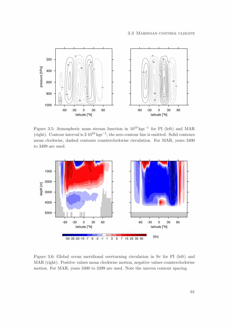
3.3 Marinoan control climate
Figure 3.5: Atmospheric mass stream function in 1010 kgs−1 for PI (left) and MAR
(right). Contour interval is 2·1010 kgs−1, the zero contour line is omitted. Solid contours
mean clockwise, dashed contours counterclockwise circulation. For MAR, years 3400
to 3499 are used.
Figure 3.6: Global ocean meridional overturning circulation in Sv for PI (left) and
MAR (right). Positive values mean clockwise motion, negative values counterclockwise
motion. For MAR, years 3400 to 3499 are used. Note the uneven contour spacing.
61
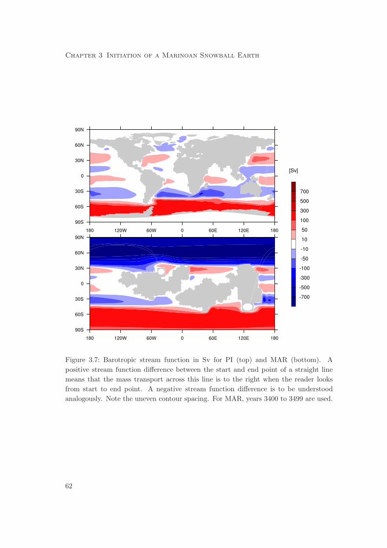
Chapter 3 Initiation of a Marinoan Snowball Earth
Figure 3.7: Barotropic stream function in Sv for PI (top) and MAR (bottom). A
positive stream function difference between the start and end point of a straight line
means that the mass transport across this line is to the right when the reader looks
from start to end point. A negative stream function difference is to be understood
analogously. Note the uneven contour spacing. For MAR, years 3400 to 3499 are used.
62
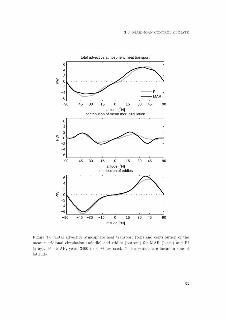
3.3 Marinoan control climate
−90 −45 −30 −15 0 15 30 45 90
−6
−4
−2
0
2
4
6
latitude [oN]
PW
total advective atmospheric heat transport
PIMAR
−90 −45 −30 −15 0 15 30 45 90
−6
−4
−2
0
2
4
6
latitude [oN]
PW
contribution of mean mer. circulation
−90 −45 −30 −15 0 15 30 45 90
−6
−4
−2
0
2
4
6
latitude [oN]
PW
contribution of eddies
Figure 3.8: Total advective atmosphere heat transport (top) and contribution of the
mean meridional circulation (middle) and eddies (bottom) for MAR (black) and PI
(gray). For MAR, years 3400 to 3499 are used. The abscissae are linear in sine of
latitude.
63
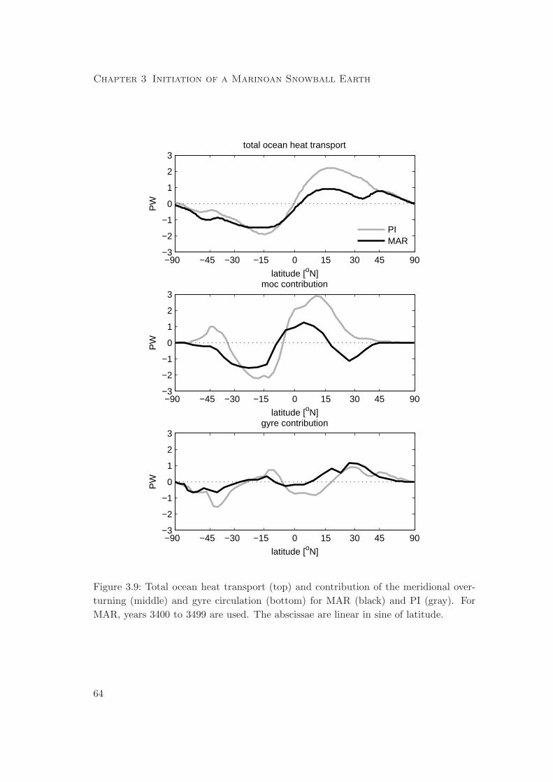
Chapter 3 Initiation of a Marinoan Snowball Earth
−90 −45 −30 −15 0 15 30 45 90−3
−2
−1
0
1
2
3
latitude [oN]
PW
total ocean heat transport
PIMAR
−90 −45 −30 −15 0 15 30 45 90−3
−2
−1
0
1
2
3
latitude [oN]
PW
moc contribution
−90 −45 −30 −15 0 15 30 45 90−3
−2
−1
0
1
2
3
latitude [oN]
PW
gyre contribution
Figure 3.9: Total ocean heat transport (top) and contribution of the meridional over-
turning (middle) and gyre circulation (bottom) for MAR (black) and PI (gray). For
MAR, years 3400 to 3499 are used. The abscissae are linear in sine of latitude.
64
3.3 Marinoan control climate
3.3.3 One-dimensional energy balance model
To gain quantitative insight into how changes in radiation and heat transport contribute
to the cold Marinoan control climate, we apply a one-dimensional energy balance model
of zonal mean surface temperature. We adapt this technique from Heinemann et al.
(2009), who used it to diagnose the causes of their simulated warm Paleocene-Eocene
climate.
Assuming equilibrium and taking the zonal mean, net incoming shortwave radia-
tion at the top of atmosphere must be balanced by outgoing longwave radiation and
divergence of meridional heat transport at each latitude (Stone 1978), i.e.
(1 − α(φ))Q(φ)) = I(φ) +H(φ) (3.1)
with
H(φ) =1
2πa2 cosφ
∂F (φ)
∂φ.
Here, α denotes the planetary albedo, Q incoming shortwave radiation at the top of
atmosphere, I outgoing longwave radiation, H divergence of time mean meridional heat
transport F ; a is Earth’s radius, φ is latitude. All quantities are understood as time
and zonal mean values as indicated by the overbar. In what follows, we will drop the
explicit notation of φ to improve readability.
If we parameterize I in terms of time and zonal mean effective emissivity ǫ and time
and zonal mean surface temperature τ ,
I = σǫτ
with Stefan-Boltzmann constant σ = 5.67 · 10−8 Wm−2K−4, we can rewrite (3.1) as
an equation for τ , and define this as the time and zonal mean surface temperature
calculated by the one-dimensional energy balance model,
τ ebm ≡ τ = 4
√
1
σǫ
{
(1 − α)Q−H
}
. (3.2)
To use this equation as a diagnostic tool for surface temperature, we need to evaluate
effective emissivity, planetary albedo, incoming shortwave radiation, and divergence of
meridional heat transport from the general circulation model. This is done by calcu-
lating these terms as
ǫ =I
I↑
s
,
α =Q
↑
Q, (3.3)
H = Q−Q↑ − I,
65
Chapter 3 Initiation of a Marinoan Snowball Earth
where I↑s is time and zonal mean longwave radiation emitted by the surface and Q
↑
the time and zonal mean shortwave radiation reflected by the planet. Both quantities
are taken from the general circulation model output. Inserting (3.3) in (3.2) yields the
one-dimensional energy balance model estimate for surface temperature, τ ebm.
The resulting surface temperature is very similar to that simulated by the general
circulation model (see Fig. 3.10). This comes as no surprise. Inserting (3.3) on the
r.h.s. of (3.2) yields
τ ebm = 4
√
1
σǫ
{
(1 − α)Q−H
}
=4
√
I↑s
σI
{
(1 − Q↑
Q)Q− (Q−Q
↑ − I)
}
=4
√
I↑
s
σ.
In the general circulation model, surface temperature and longwave radiation emitted
by the surface at each time step t and grid point (λ, φ) are related by
I↑s (t, λ, φ) = ǫστ4gcm(t, λ, φ), (3.4)
with the close to unity constant ǫ taking into account the deviation of Earth’s surface
from a perfect black body. Note that in (3.4), Is↑(t, λ, φ) and τ4
gcm(t, λ, φ) are not
time and zonal mean values. The surface temperature calculated by the energy balance
model, τ ebm, therefore is related to the actual time and zonal mean surface temperature
of the general circulation model via
τ ebm =4√ǫ 4
√
τ4gcm(t, λ, φ).
The difference between the surface temperature diagnosed by the energy balance model
and the time and zonal mean surface temperature of the general circulation model,
τ ebm − τgcm, consequently is, apart from the small and globally constant offset by4√ǫ ≃ 1, only due to the non-permutability of taking the fourth root and taking the
time and zonal mean,
τ ebm − τgcm =4√ǫ 4
√
τ4gcm(t, λ, φ) − τgcm(t, λ, φ).
In other words, the difference between the one-dimensional energy balance model and
the general circulation model is only caused by time and zonal variations of surface
temperature.
The one-dimensional energy balance barely helps to understand why a particular
simulated climate is as warm or cold as it is. Its power lies in analyzing the reasons for
66
3.3 Marinoan control climate
the surface temperature difference between two climate simulations by separating how
much change of surface temperature is caused by changes in planetary albedo, effective
emissivity, and meridional heat transport (for simplicity we here assume that incoming
shortwave radiation at the top of atmosphere is the same in the two climate simulations;
for MAR and PI this condition is fulfilled). This is done in the following way. Given PI
and MAR, we calculate (3.3) for each simulation separately. Each simulation satisfies
(3.2) with its respective set of diagnosed radiation and heat transport parameters,
τPIebm = 4
√
1
σǫPI
{
(1 − αPI)Q−HPI
}
,
τMARebm = 4
√
1
σǫMAR
{
(1 − αMAR)Q−HMAR
}
.
Following Heinemann et al. (2009), we estimate the surface temperature change from
PI to MAR caused by changes in planetary albedo by
△τ∣
∣
∣
∣
α
= 4
√
1
σǫPI
{
(1 − αMAR)Q−HPI
}
− τPIebm.
The effect of changes in effective emissivity and divergence of meridional heat transport
are given analogously by
△τ∣
∣
∣
∣
ǫ
= 4
√
1
σǫMAR
{
(1 − αPI)Q−HPI
}
− τPIebm
and
△τ∣
∣
∣
∣
H
= 4
√
1
σǫPI
{
(1 − αPI)Q−HMAR
}
− τPIebm.
This approach is justified by the fact that the sum of the individual estimates (see
below) does nowhere deviate from the total temperature change by more than 0.2 K.
According to Fig. 3.10, the increased planetary albedo in MAR leads to a cooling
compared to PI at all latitudes. The only exception is the South Pole region where the
replacement of the Antarctic glacier by sea ice results in a slight decrease of surface
albedo, which translates to a small planetary albedo warming effect. The sign of MAR -
PI surface temperature changes induced by effective emissivity and meridional heat
transport depend on latitude. In the tropics, reduced divergence of meridional heat
transport and reduced effective emissivity have a warming effect in MAR compared to
PI and offset a significant bit of the albedo induced cooling. In midlatitudes, planetary
albedo, effective emissivity and meridional heat transport all contribute to the simulated
cooling in MAR, with nearly equal partitioning between the three in the Southern
Hemisphere. In Northern Hemisphere polar latitudes, the cooling in MAR is equally
67
Chapter 3 Initiation of a Marinoan Snowball Earth
generated by higher planetary albedo and higher effective emissivity with heat transport
changes only becoming important close to the North Pole. This picture is similar for
Southern Hemisphere polar latitudes north of today’s Antarctic continent. Close to the
South Pole, increased effective emissivity and convergence of meridional heat transport
result in a warming, similar to planetary albedo.
The global cooling effect of planetary albedo changes is consistent with what one
expects from clustering continents with comparably high surface albedo in the tropics
and increasing sea-ice cover in the extratropics. The tropical warming effect of effective
emissivity changes is counter to the expected effect of the strong reduction of water
vapor in MAR and hence must be related to clouds. Moreover, it is unclear from this
analysis whether, for example, the tropical warming effect of heat transport changes
is due to changes in atmosphere or ocean (including sea-ice) heat transport. To an-
swer these issues, the above diagnostics are expanded to separate cloud and clear-sky
radiative effects as well as the effects of atmosphere and ocean heat transports.
The temperature effect of cloud changes is isolated from that of surface albedo
changes, in the case of planetary albedo, and water vapor changes, in the case of
effective emissivity, by virtue of full-sky and clear-sky radiative fluxes. The time and
zonal mean planetary albedo can be decomposed into the clear-sky planetary albedo
αcs, which to good approximation equals surface albedo, and the contribution of clouds
to planetary albedo, αcl,
α = αcs + αcl.
Note that αcl does not equal the cloud albedo but measures the importance of clouds
for planetary albedo. In an analogous manner, effective emissivity is split into clear-sky
emissivity, ǫcs, mainly depending on water vapor content, and again cloud contribution,
ǫcl,
ǫ = ǫcs + ǫcl.
Clear-sky albedo and effective emissivity are diagnosed from the general circulation
model as
ǫcs =Ics
I↑
s
,
αcs =Q
↑cs
Q,
with subscript cs meaning that now clear-sky radiative fluxes are used. The cloud con-
tributions are calculated as residuals between full-sky and clear-sky values. Atmosphere
and ocean meridional heat transport divergences are separated by means of the the time
and zonal mean surface heat flux V s, which is computed from the general circulation
model as the time and zonal mean sum of surface shortwave and longwave radiation
68
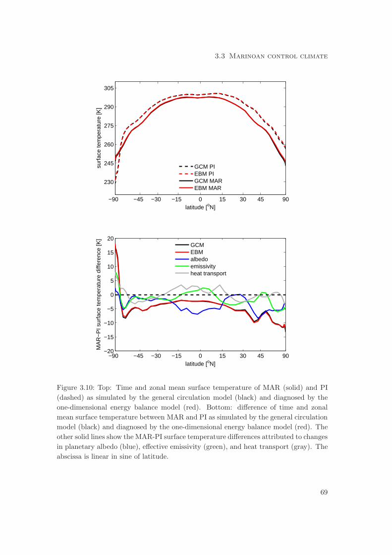
3.3 Marinoan control climate
−90 −45 −30 −15 0 15 30 45 90
230
245
260
275
290
305
latitude [oN]
surf
ace
tem
pera
ture
[K]
GCM PIEBM PIGCM MAREBM MAR
−90 −45 −30 −15 0 15 30 45 90−20
−15
−10
−5
0
5
10
15
20
latitude [oN]
MA
R−
PI s
urfa
ce te
mpe
ratu
re d
iffer
ence
[K]
GCMEBMalbedoemissivityheat transport
Figure 3.10: Top: Time and zonal mean surface temperature of MAR (solid) and PI
(dashed) as simulated by the general circulation model (black) and diagnosed by the
one-dimensional energy balance model (red). Bottom: difference of time and zonal
mean surface temperature between MAR and PI as simulated by the general circulation
model (black) and diagnosed by the one-dimensional energy balance model (red). The
other solid lines show the MAR-PI surface temperature differences attributed to changes
in planetary albedo (blue), effective emissivity (green), and heat transport (gray). The
abscissa is linear in sine of latitude.
69
Chapter 3 Initiation of a Marinoan Snowball Earth
fluxes, the sensible heat flux, and the latent heat flux. With this, the meridional heat
transport divergence due to the atmosphere is given by
Ha = H − V s,
and that due to the ocean (including sea-ice) by
Ho = H −Ha = V s.
The effect of clear-sky albedo changes between MAR and PI on surface temperatures
is calculated as for planetary albedo but with cloud contribution kept at its PI value,
i.e.
△τ∣
∣
∣
∣
αcs
= 4
√
1
σǫPI
{
(1 − αcs,MAR − αcl,PI)Q−HPI
}
− τPIebm.
For the effect of planetary albedo changes due to cloud changes, we have
△τ∣
∣
∣
∣
αcl
= 4
√
1
σǫPI
{
(1 − αcs,PI − αcl,MAR)Q−HPI
}
− τPIebm.
The effect of changes in clear-sky effective emissivity, cloud contribution to effective
emissivity, and meridional heat transport divergence due to atmosphere and ocean are
computed analogously.
Changes in clear-sky planetary albedo lead to cooling in MAR everywhere except
in Northern midlatitudes, where the reduced land fraction in MAR compared to PI
effects a decreased surface albedo and hence decreased clear-sky planetary albedo (Fig.
3.11). The temperature effect of changes in the cloud contribution is opposite to the
temperature effect of changes in clear-sky planetary albedo. At most latitudes, clouds
contribute less to planetary albedo in MAR than in PI because of the increased surface
albedo in MAR (see Fig. 3.4). This translates to a warming effect of the cloud contribu-
tion. In Northern midlatitudes, however, the decreased surface albedo in MAR effects
that clouds can contribute more to planetary albedo in MAR than in PI. Supported
by the increased cloud cover at these latitudes in MAR (see Fig. 3.4), this means that
changes in the cloud contribution to planetary albedo have a cooling effect in Northern
midlatitudes. This cooling is even larger than the warming due to increased clear-sky
surface albedo such that also in Northern midlatitudes, planetary albedo in MAR is
higher than in PI, implying a cooling effect by increased planetary albedo. For effective
emissivity, clear-sky emissivity is higher in MAR than PI, consistent with the reduction
in water vapor content (cf. Fig. 3.12). Clear-sky effective emissivity changes therefore
have a cooling effect in MAR, except close to the South Pole. Cloud changes mainly
have a warming effect, such that the overall surface temperature decrease from PI to
MAR due to changing effective emissivity is smaller than that from reduced water va-
por content alone. In the tropics, cloud warming even offsets the cooling by increased
70
3.3 Marinoan control climate
clear-sky effective emissivity, showing that the tropical warming effect of changes in ef-
fective emissivity is caused by cloud changes. Surface temperature changes attributed
to changes of total meridional heat transport result from strong and largely opposite
changes in atmosphere and ocean heat transports. In the tropics, the warming effect
is caused by less divergence of ocean heat transport, visible in a flatter shape of trop-
ical total implied ocean heat transport in MAR compared to PI (Fig. 3.13). This
seems plausible from a smaller tropical ocean fraction in MAR. The most pronounced
change of surface temperature due to changes in ocean heat transport is a 17 K cooling
around 35◦ N. This strong local cooling effect is related to a drastic change in the ocean
meridional overturning circulation around 35◦ N in MAR compared to PI (see above).
Changes of atmospheric heat transport, however, offset this cooling almost completely.
That large temperature changes attributed to changes in atmosphere and ocean heat
transport mainly compensate can be understood from the fact that the divergence of
total meridional heat transport, or equivalently the sum of shortwave and longwave
radiation at the top of atmosphere, has an as gentle shape in MAR as in PI.
Finally, we quantify the changes of planetary albedo, effective emissivity and heat
transport contribute to the total change of global mean surface temperature. This is
done by meridionally averaging the latitudinal contributions (Tab. 3.4). We find that
two thirds of the global mean cooling of 4.6 K from PI to MAR are caused by increased
planetary albedo and the remaining one third by increased effective emissivity, that
is a weaker greenhouse effect. Clouds reduce the cooling that would result from the
expansion of sea ice and the reduction of water vapor alone. This does not imply
a positive total cloud radiative forcing in MAR, but means that total cloud radiative
forcing is less negative in MAR than in PI (see Tab. 3.3). The global mean temperature
change due to changes in the divergence of heat transport is negligible.
71
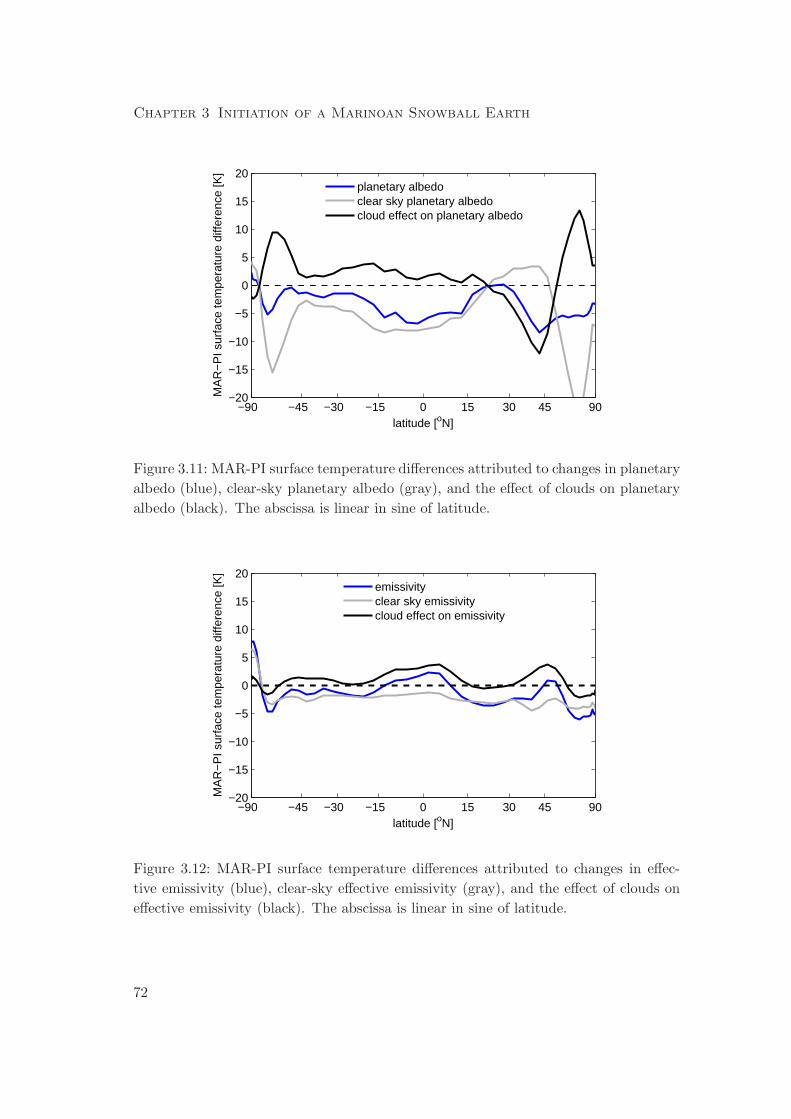
Chapter 3 Initiation of a Marinoan Snowball Earth
−90 −45 −30 −15 0 15 30 45 90−20
−15
−10
−5
0
5
10
15
20
latitude [oN]
MA
R−
PI s
urfa
ce te
mpe
ratu
re d
iffer
ence
[K]
planetary albedoclear sky planetary albedocloud effect on planetary albedo
Figure 3.11: MAR-PI surface temperature differences attributed to changes in planetary
albedo (blue), clear-sky planetary albedo (gray), and the effect of clouds on planetary
albedo (black). The abscissa is linear in sine of latitude.
−90 −45 −30 −15 0 15 30 45 90−20
−15
−10
−5
0
5
10
15
20
latitude [oN]
MA
R−
PI s
urfa
ce te
mpe
ratu
re d
iffer
ence
[K]
emissivityclear sky emissivitycloud effect on emissivity
Figure 3.12: MAR-PI surface temperature differences attributed to changes in effec-
tive emissivity (blue), clear-sky effective emissivity (gray), and the effect of clouds on
effective emissivity (black). The abscissa is linear in sine of latitude.
72
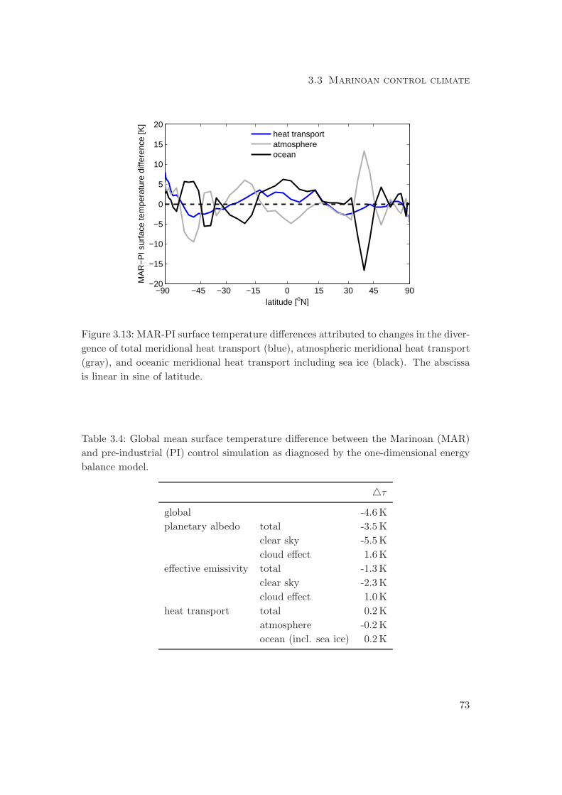
3.3 Marinoan control climate
−90 −45 −30 −15 0 15 30 45 90−20
−15
−10
−5
0
5
10
15
20
latitude [oN]
MA
R−
PI s
urfa
ce te
mpe
ratu
re d
iffer
ence
[K]
heat transportatmosphereocean
Figure 3.13: MAR-PI surface temperature differences attributed to changes in the diver-
gence of total meridional heat transport (blue), atmospheric meridional heat transport
(gray), and oceanic meridional heat transport including sea ice (black). The abscissa
is linear in sine of latitude.
Table 3.4: Global mean surface temperature difference between the Marinoan (MAR)
and pre-industrial (PI) control simulation as diagnosed by the one-dimensional energy
balance model.
△τ
global -4.6 K
planetary albedo total -3.5 K
clear sky -5.5 K
cloud effect 1.6 K
effective emissivity total -1.3 K
clear sky -2.3 K
cloud effect 1.0 K
heat transport total 0.2 K
atmosphere -0.2 K
ocean (incl. sea ice) 0.2 K
73
Chapter 3 Initiation of a Marinoan Snowball Earth
3.4 Snowball Earth bifurcation point and maximum stable
sea-ice cover
This sections reports on the effect of an abrupt decrease of total solar irradiance and,
for some simulations, simultaneous increase of atmospheric carbon dioxide. These sim-
ulations enable us to find the Snowball Earth bifurcation point as well as the maximum
stable sea-ice cover.
Virtually switching off the sun results in global sea-ice cover within 9 years (simu-
lation TSI00, not shown). A reduction of TSI to 94% of its present-day value leads
to a Snowball Earth within 354 years (simulation TSI94, see Fig. 3.14). In TSI94, the
sea-ice line is nearly symmetric about the equator during the entire transition, and
snow accumulates in the Southern but not in the Northern Hemisphere. While surface
albedo increases in the Northern Hemisphere are hence solely due to the conversion of
open ocean areas to sea ice, snow accumulation on land contributes to surface albedo
increases in the Southern Hemisphere. The surface albedo of the Southern Hemisphere
consequently increases at the same rate as the Northern Hemisphere surface albedo,
and meridional heat transports stay symmetric about the equator during the entire
transition (not shown). This is in contrast to the initiation of a modern Snowball
Earth (Voigt and Marotzke 2009), where the asymmetric distribution of continents
between the Northern and Southern Hemisphere, combined with virtually zero snow-
accumulation on land, caused a much faster increase of surface albedo in the Southern
Hemisphere than in the Northern Hemisphere, and by this strong heat transport toward
the more water-covered Southern hemisphere as sea ice spread towards the equator.
In contrast to a reduction of TSI to 94%, decreasing TSI to 96% does not effect global
sea-ice cover (simulation TSI96). Sea-ice expansion in this simulation is initially almost
as fast as for a TSI reduction to 94%, but decelerates 250 years after the TSI decrease.
A further 1000 years later, sea-ice area stabilizes at 20·1013 m2, equivalent to 55% of
the Marinoan ocean surface area. To further pin down the Marinoan Snowball Earth
bifurcation point, we branch off simulation TSI-955 from year 5799 of TSI96. In this
simulation, total solar irradiance is additionally decreased by 6.8 Wm−2 to 95.5% of its
present-day value. This small additional TSI reduction is sufficient to induce global
sea-ice cover within 200 years. The Snowball Earth bifurcation point, for pre-industrial
levels of carbon dioxide, therefore is between 95.5 and 96% of the present-day total
solar irradiance.
That we are able to fix the Snowball Earth bifurcation within an uncertainty of 0.5%
of the present-day TSI also enables us to infer the maximum stable sea-ice area. As
shown by TSI96, sea ice can cover 55% of the ocean surface area without triggering a
climate instability. At the end of TSI96, the sea-ice line has stabilized at 30◦ N and
around 25◦ S, respectively (Fig. 3.15), with sea-ice being snow-covered except very
close to the sea-ice edge, and snow on land restricted to largely thin snow cover in the
74
3.4 Snowball Earth bifurcation point
southernmost parts of Gondwana. The strong sensitivity of this sea-ice line to the small
reduction in TSI demonstrates that equilibrium solutions with sea-ice cover above 55%
are highly unlikely, or if they occur, highly unstable.
Falling into a Snowball Earth when TSI is reduced to 94% is prevented by an appro-
priate increase in atmospheric carbon dioxide. Combining a reduction of TSI to 94%
with a quadrupling of atmospheric carbon dioxide with respect to its pre-industrial
level results in an increase of the sea-ice area to 14·1013 m2, corresponding to 37% of
the Marinoan ocean surface area (simulation TSI94-4CO2). Therefore, for total so-
lar irradiance at 94% of its present-day value, i.e. the value commonly assumed for
the Marinoan, the Snowball Earth bifurcation is between one and four times the pre-
industrial concentration of carbon dioxide. Increasing carbon dioxide even further to 6
times its pre-industrial level almost compensates for the decrease of TSI to 94% (sim-
ulation TSI94-6CO2). After 1000 years, sea-ice area in this case is only slightly higher
than in the control simulation MAR though ocean potential temperatures still decline.
Reducing TSI to 94% and quadrupling carbon dioxide has almost the same effect on
sea-ice area as reducing TSI to 98%. This is consistent with the fact that the radiative
forcing of increasing TSI by 4% and assuming a planetary albedo of 0.353 as simulated
for MAR,
RF(4%TSI0) = (1 − 0.353) · 0.041367
4Wm−2 = 8.8 Wm−2,
is close to the radiative forcing of quadrupling carbon dioxide (Myhre et al. 1998),
RF(4 × CO2) = 5.35 ln 4 Wm−2 = 7.4 Wm−2.
Note that if we took into account that the planetary albedo increases in the course of
TSI98 and TSI94-4CO2, we would obtain a slightly lower radiative forcing estimate for
the 4% reduction in TSI, bringing the two estimates closer together. Moreover, the
factor of 5.35 used in the radiative forcing estimate of quadrupling carbon dioxide is
valid for present-day conditions but might be different for the Marinoan.
Simulation TSI100 is started from year 3999 of TSI94 with TSI set back to 100%. As
one expects, this 6% increase does not lead to Snowball Earth deglaciation and sea-ice
cover remains global in TSI100 (not shown). This establishes that, akin to present-
day conditions (Marotzke and Botzet 2007), ECHAM5/MPI-OM exhibits bistability
for TSI at its present-day value also in the Marinoan setup.
75
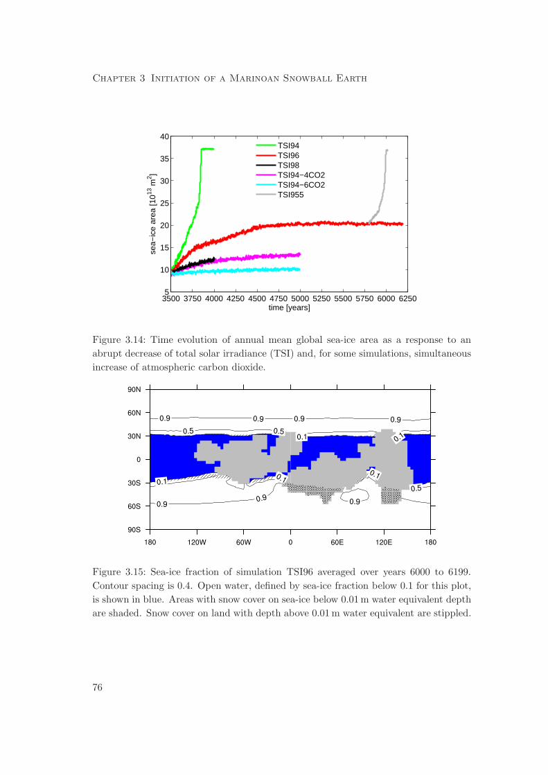
Chapter 3 Initiation of a Marinoan Snowball Earth
3500 3750 4000 4250 4500 4750 5000 5250 5500 5750 6000 62505
10
15
20
25
30
35
40
time [years]
sea−
ice
area
[1013
m2 ]
TSI94TSI96TSI98TSI94−4CO2TSI94−6CO2TSI955
Figure 3.14: Time evolution of annual mean global sea-ice area as a response to an
abrupt decrease of total solar irradiance (TSI) and, for some simulations, simultaneous
increase of atmospheric carbon dioxide.
Figure 3.15: Sea-ice fraction of simulation TSI96 averaged over years 6000 to 6199.
Contour spacing is 0.4. Open water, defined by sea-ice fraction below 0.1 for this plot,
is shown in blue. Areas with snow cover on sea-ice below 0.01 m water equivalent depth
are shaded. Snow cover on land with depth above 0.01 m water equivalent are stippled.
76
3.5 Prediction of the Snowball Earth bifurcation point by a 0-d EBM
3.5 Prediction of the Snowball Earth bifurcation point and
transition times by a zero-dimensional energy balance
model
For the initiation of a modern Snowball Earth, Voigt and Marotzke (2009) showed that
the Snowball Earth bifurcation point estimated with the atmosphere-ocean general
circulation model and the transition times are well reproduced by a zero-dimensional
energy balance model (EBM) of global mean ocean potential temperature. In Voigt and
Marotzke (2009), however, the Snowball Earth bifurcation point was only established
within an accuracy of 3% of the present-day total solar irradiance. This raises the
question if this EBM still agrees with the here much more precise estimate of the
bifurcation point for Marinoan surface boundary conditions.
We start with a review of the EBM described in Voigt and Marotzke (2009), including
the details of solving the model and determining its parameters. The latter were not
given in Voigt and Marotzke (2009). By neglecting atmosphere and land and consid-
ering the ocean to be perfectly mixed, the EBM predicts the evolution of mean ocean
potential temperature θ in response to a decrease in total solar irradiance according to
cdθ
dt=
(1 − α)
4TSI − ǫσθ4. (3.5)
Here, c = 1.52 · 1010 JK−1m−2 denotes the ocean heat capcity per unit surface area,
and σ = 5.67 · 10−8 the Stefan-Boltzmann constant. The parameter α can be thought
of as the global mean planetary albedo while ǫ takes into account the greenhouse effect.
Eq. (3.5) can be integrated by separation of variables and the help of an integral table
(Bronstein 1996) to yield an implicit equation for θ at time t after the abrupt reduction
of solar irradiance from TSI0=1367 Wm−2 to TSI<TSI0 at t = 0,
1
4(β TSI)3/4ln
∣
∣
∣
∣
(β TSI)1/4 + θ(t,TSI)
(β TSI)1/4 − θ(t,TSI)
∣
∣
∣
∣
+1
2(β TSI)3/4arctan
{
θ(t,TSI)
(β TSI)1/4
}
= γ(t+ δ)
The transition to a Snowball Earth in the EBM is accomplished as soon as θ drops to
the freezing temperature of sea water, θf = 271.25 K. The transition time to a Snowball
Earth is therefore given by the time tf (TSI) at which θ = θf ,
tf (TSI) =1
4γ(β TSI)3/4ln
∣
∣
∣
∣
(β TSI)1/4 + θf
(β TSI)1/4 − θf
∣
∣
∣
∣
+1
2γ(β TSI)3/4arctan
{
θf
(β TSI)1/4
}
− δ.
(3.6)
To apply (3.6) in practice, we need to determine the parameters β, γ, and δ. The
latter, δ, is defined by the initial condition that at the instant of TSI reduction, t = 0,
the ocean potential temperature equals the equilibrium ocean potential temperature
77
Chapter 3 Initiation of a Marinoan Snowball Earth
for today’s total solar irradiance, i.e. θ(0,TSI) = θMAR = 274.3 K. This yields
δ(TSI) =1
γ
{
1
4(β TSI)3/4ln
∣
∣
∣
∣
(β TSI)1/4 + θMAR
(β TSI)1/4 − θMAR
∣
∣
∣
∣
+1
2(β TSI)3/4arctan
{
θMAR
(βTSI)1/4
}
}
.
The parameter β abbreviates
β =1 − α
4σǫ
and is determined by the tuneable ratio of 1−α and ǫ. This ratio is fixed by requiring
that the Marinoan control climate is an equilibrium solution of (3.5),
1 − α
ǫ= 4σ
θ4MAR
TSI0≃ 0.9392. (3.7)
For the parameter γ, which is an abbreviation for
γ =σǫ
c,
we need to evaluate ǫ. This is done by demanding that the EBM reproduces the 9
year transition time of the atmosphere-ocean general circulation model for virtually
switching off the sun (simulation TSI00). In this case, the TSI term drops out of (3.5)
and, after some algebra, we obtain
ǫ =c
3σtf (TSI00)
{
1
θ3f
− 1
θ3MAR
}
= 0.5200,
where tf (TSI00) = 9 a.
By construction, the transition time of the EBM agrees with that of the general
circulation model for TSI set to virtually zero (Fig. 3.16). For TSI set to 94% of its
present-day value the EBM slightly underestimates the transition time; the EBM gives
264 years instead of the 354 years found with the atmosphere-ocean general circulation
model (simulation TSI94). For TSI ≥ 1307 Wm−2 = 95.63% TSI0 global mean ocean
potential temperature in the EBM never falls below the freezing point of sea water. The
EBM therefore estimates the Snowball Earth bifurcation point to 95.63% TSI0. This is
in intriguing agreement with the 95.5 to 96% range found with the atmosphere-ocean
general circulation model.
Since the estimate of the Snowball Earth bifurcation point is defined as the total solar
irradiance TSIc needed to cool θ to θf in the limit t → ∞, examining the individual
terms of the r.h.s. of (3.6) gives a formula for the EBM’s estimate of the Snowball Earth
bifurcation point. Obeying that β, γ, δ,TSI, θf , and the arctan-term are all finite, we
see that the only way to generate an infinity on the r.h.s. of (3.6) is through
(β TSIc)1/4 − θf = 0. (3.8)
78
3.5 Prediction of the Snowball Earth bifurcation point by a 0-d EBM
The EBM’s estimate of the Snowball Earth bifurcation point is therefore determined
by
TSIc =θ4f
β=
(
θf
θMAR
)4
TSI0. (3.9)
TSIc is completely fixed by the equilibrium global mean ocean potential temperature
for today’s total solar irradiance. The warmer the control climate for TSI0, the larger
the TSI reduction needed for Snowball Earth initiation. This was already mentioned
by Voigt and Marotzke (2009), but we here demonstrate this fact explicitly.
Estimating the Snowball Earth bifurcation point actually does not require to calcu-
late the time-evolution of θ(t,TSI). Since in the limit t → ∞ the EBM approaches
equilibrium, TSIc is constrained by
(1 − α)
4TSIc = ǫσθ4
f (3.10)
This again yields
TSIc =4ǫσ
(1 − α)θ4f =
(
θf
θMAR
)4
TSI0.
What ultimately only is important for the EBM’s estimate of the Snowball Earth
bifurcation point is the assumption that the ratio (1 − α)/ǫ is the same for TSI0 and
TSIc, and all TSI values in between. Since a TSI reduction triggers sea-ice expansion
and by this an increased planetary albedo, this assumption implies a decrease of ǫ with
reduced TSI. At first glance, the latter seems incompatible with decreased atmospheric
water-vapor in a colder climate. However, this conflict is dissolved by acknowledging
that in order to compare the EBM parameter ǫ with the effective emissivity ǫgcm that is
diagnosed from the atmosphere-ocean general circulation model, we need to incorporate
the formfactor (SST/θ)4 (Voigt and Marotzke 2009). This factor takes into account
that the EBM parameterizes longwave radiation energy loss through the global mean
ocean potential temperature instead of global mean sea surface temperature SST. This
yields
ǫ = ǫgcm
(
SST
θ
)4
.
While the effective emissivity ǫgcm increases with decreased TSI, the EBM parameter
ǫ can still decrease because decreased TSI also reduces ocean stratification (Voigt and
Marotzke 2009). This justifies the assumption that the ratio (1 − α)/ǫ stays constant
when TSI is reduced to or above the Snowball Earth bifurcation point TSIc.
Finally, the fact that the considered values of θ are close to θf suggests to linearize
(3.5) at θf . Doing so allows us to derive a much simpler but essentially as good estimate
for the transition times as obtained by solving the non-linear equation (3.5). If we write
θ(t,TSI) = θf + T (t,TSI),
79
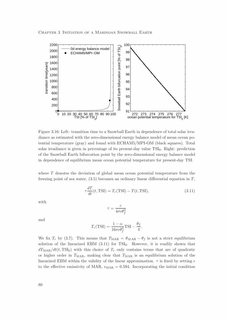
Chapter 3 Initiation of a Marinoan Snowball Earth
0 10 20 30 40 50 60 70 80 90 1000
200
400
600
800
1000
1200
1400
1600
1800
2000
2200
TSI [% of TSI0]
tran
sitio
n tim
e[ye
ars]
0d energy balance modelECHAM5/MPI−OM
272 273 274 275 276 27791
92
93
94
95
96
97
98
99
100
ocean potential temperature for TSI0 [K]
Sno
wba
ll E
arth
bifu
rcat
ion
poin
t [%
of T
SI 0]
Figure 3.16: Left: transition time to a Snowball Earth in dependence of total solar irra-
diance as estimated with the zero-dimensional energy balance model of mean ocean po-
tential temperature (gray) and found with ECHAM5/MPI-OM (black squares). Total
solar irradiance is given in percentage of its present-day value TSI0. Right: prediction
of the Snowball Earth bifurcation point by the zero-dimensional energy balance model
in dependence of equilibrium mean ocean potential temperature for present-day TSI.
where T denotes the deviation of global mean ocean potential temperature from the
freezing point of sea water, (3.5) becomes an ordinary linear differential equation in T ,
τdT
dt(t,TSI) = Tr(TSI) − T (t,TSI), (3.11)
with
τ =c
4σǫθ3f
and
Tr(TSI) =1 − α
16σǫθ3f
TSI − θf
4.
We fix Tr by (3.7). This means that TMAR = θMAR − θf is not a strict equilibrium
solution of the linearized EBM (3.11) for TSI0. However, it is readily shown that
dTMAR/dt(t,TSI0) with this choice of Tr only contains terms that are of quadratic
or higher order in TMAR, making clear that TMAR is an equilibrium solution of the
linearized EBM within the validity of the linear approximation. τ is fixed by setting ǫ
to the effective emissivity of MAR, ǫMAR = 0.594. Incorporating the initial condition
80
3.6 Energy fluxes at the top of atmosphere and at the surface
T (t = 0,TSI) = TMAR, (3.11) is solved by
T (t,TSI) = Tr(TSI) + {TMAR − Tr(TSI)} exp(−t/τ).
The transition time to a Snowball Earth estimated with the linearized EBM, tlinf (TSI),
is defined by T (tf ,TSI) = 0. We obtain
tlinf (TSI) = τ lnTr(TSI) − TMAR
Tr(TSI).
For switched-off sun, the linearised EBM gives a transition time of 8 years. This is in
very good agreement with the GCM, in particular since no explicit tuning of ǫ is applied
for the linear EBM. The transition time for TSI=94% TSI0 is 232 years, slightly less
than the estimate of 264 years of the non-linear EBM. When plotted in Fig. 3.16, the
transition time of the linear EBM would be indistinguishable from that of the non-linear
EBM.
3.6 Energy fluxes at the top of atmosphere and at the surface
For an atmosphere in equilibrium, energy conservation requires that the global mean
energy flux at the top of atmosphere, Ftoa, given by the sum of net incoming shortwave
radiation and outgoing longwave radiation, equals the global mean energy flux at the
surface Fsfc, the latter given by the sum of surface shortwave and longwave radiation
and latent and sensible heat fluxes.
We have checked to which degree this is fullfilled in our simulations. For the Marinoan
control simulation MAR, the top of atmosphere energy flux is 0.7 Wm−2 larger than
the surface energy flux (Fig. 3.17). This imbalance is close to the 0.5 Wm−2 imbalance
that we find for the pre-industrial control simulation PI.
In contrast, the top of atmosphere and the surface energy fluxes differ much more
in an equilibrium Snowball Earth state. For example, when total solar irradiance
is set to 94% of its today’s value, the imbalance amounts to -5 Wm−2 (Fig. 3.17).
Now, the atmosphere loses more energy at the top of atmosphere than it gains at the
surface, suggesting that an artificial energy source exists in the atmosphere model.
If we use the global integral of atmospheric energy content of today’s atmosphere,
Hatm = 256 · 107 Jm−2 (Peixoto and Oort 1992), as an estimate for atmospheric energy
content of the equilibrium Snowball Earth atmosphere, we find that this imbalance
accumulates to the total atmospheric energy content within
Hatm
Ftoa − Fsfc
≃ 16 a.
The reason for the much larger imbalance in an equilibrium Snowball Earth is obscure
to us, as well as the reason why the imbalance changes sign from the control simulations
MAR and PI to the equilibrium simulation of a Snowball Earth.
81
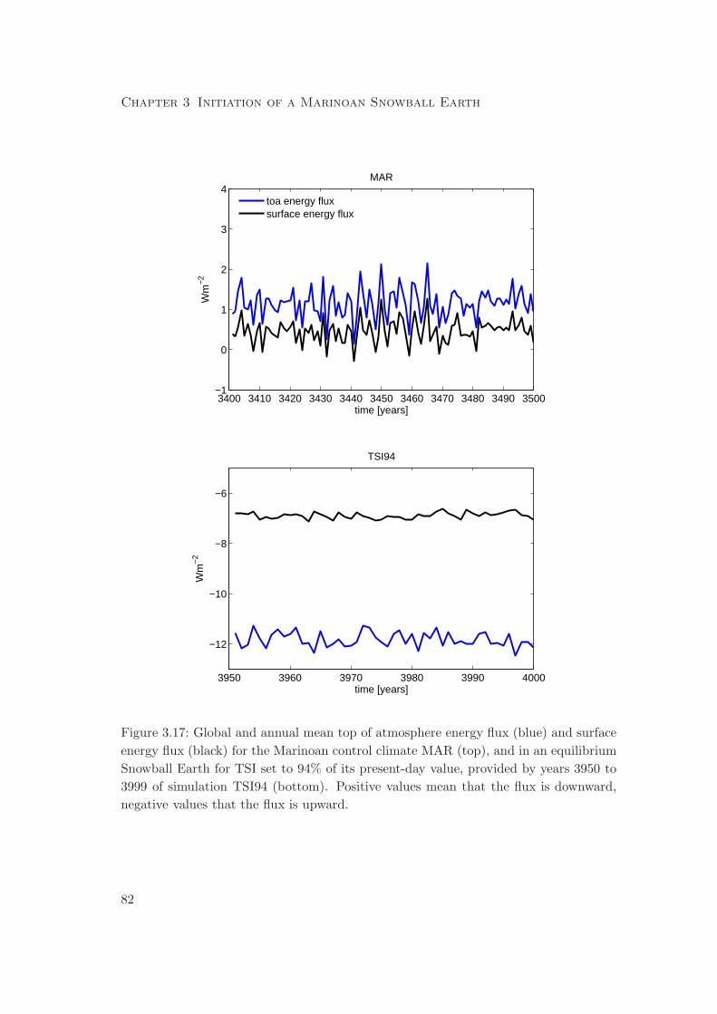
Chapter 3 Initiation of a Marinoan Snowball Earth
3400 3410 3420 3430 3440 3450 3460 3470 3480 3490 3500−1
0
1
2
3
4
time [years]
Wm
−2
MAR
toa energy fluxsurface energy flux
3950 3960 3970 3980 3990 4000
−12
−10
−8
−6
TSI94
time [years]
Wm
−2
Figure 3.17: Global and annual mean top of atmosphere energy flux (blue) and surface
energy flux (black) for the Marinoan control climate MAR (top), and in an equilibrium
Snowball Earth for TSI set to 94% of its present-day value, provided by years 3950 to
3999 of simulation TSI94 (bottom). Positive values mean that the flux is downward,
negative values that the flux is upward.
82
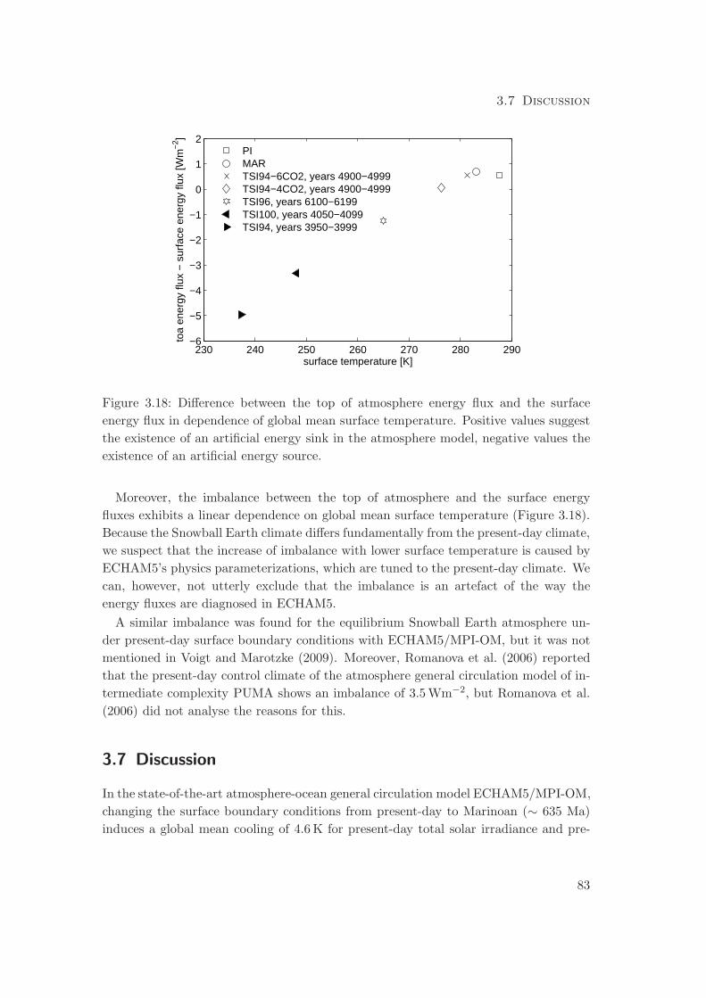
3.7 Discussion
230 240 250 260 270 280 290−6
−5
−4
−3
−2
−1
0
1
2
surface temperature [K]
toa
ener
gy fl
ux −
sur
face
ene
rgy
flux
[Wm
−2 ]
PIMARTSI94−6CO2, years 4900−4999TSI94−4CO2, years 4900−4999TSI96, years 6100−6199TSI100, years 4050−4099TSI94, years 3950−3999
Figure 3.18: Difference between the top of atmosphere energy flux and the surface
energy flux in dependence of global mean surface temperature. Positive values suggest
the existence of an artificial energy sink in the atmosphere model, negative values the
existence of an artificial energy source.
Moreover, the imbalance between the top of atmosphere and the surface energy
fluxes exhibits a linear dependence on global mean surface temperature (Figure 3.18).
Because the Snowball Earth climate differs fundamentally from the present-day climate,
we suspect that the increase of imbalance with lower surface temperature is caused by
ECHAM5’s physics parameterizations, which are tuned to the present-day climate. We
can, however, not utterly exclude that the imbalance is an artefact of the way the
energy fluxes are diagnosed in ECHAM5.
A similar imbalance was found for the equilibrium Snowball Earth atmosphere un-
der present-day surface boundary conditions with ECHAM5/MPI-OM, but it was not
mentioned in Voigt and Marotzke (2009). Moreover, Romanova et al. (2006) reported
that the present-day control climate of the atmosphere general circulation model of in-
termediate complexity PUMA shows an imbalance of 3.5 Wm−2, but Romanova et al.
(2006) did not analyse the reasons for this.
3.7 Discussion
In the state-of-the-art atmosphere-ocean general circulation model ECHAM5/MPI-OM,
changing the surface boundary conditions from present-day to Marinoan (∼ 635 Ma)
induces a global mean cooling of 4.6 K for present-day total solar irradiance and pre-
83
Chapter 3 Initiation of a Marinoan Snowball Earth
industrial greenhouse gas concentrations. Although the Marinoan surface boundary
conditions are distinct from the present-day surface boundary conditions in more as-
pects than the location of continents, we consider the latter as the primary difference
between the two setups. The movement of continents from high to low latitudes ac-
cording to the Marinoan reconstruction results in a redistribution of background surface
albedo across the globe, with higher low latitude surface albedo in the Marinoan than
today. By virtue of the larger incoming shortwave radiation in low latitudes, this implies
a cooling of the climate.
This cooling entails that a Snowball Earth is much easier generated for Marinoan
than for present-day surface boundary conditions. For the latter a reduction of TSI to
94% did not result in a Snowball Earth (Voigt and Marotzke 2009), whereas we find it
to be sufficient for the Marinoan setup. Our simulations hence support the notion that
low-latitude continents facilitate global glaciation (Kirschvink 1992). This confirms
the result of Lewis et al. (2003), but is in disagreement with the opposite conclusion
of Poulsen et al. (2002). In the latter study with the Fast Ocean Atmosphere Model
(FOAM), changing continents from a Southern Hemisphere preponderance to equatorial
supercontinent(s) effected a global warming of about 5K.
A zero-dimensional energy balance model successfully predicts the Snowball Earth
bifurcation point in terms of total solar irradiance by only knowing the equilibrium
global mean ocean potential temperature for present-day total solar irradiance and
pre-industrial greenhouse gases. The model has shown this ability before for present-
day conditions and here confirms it in an intriguing manner. It would be interesting
to see if the model in simulations with different continental setups or climate models
performs equally well. However, the energy balance model in its current form does not
predict the Snowball Earth bifurcation point in terms of carbon dioxide.
Sea-ice advance during the transition to a Marinoan Snowball Earth is symmetric
about the equator, in contrast to the transition to a modern Snowball Earth with
present-day geography (Voigt and Marotzke 2009). This confirms that continents via
their albedo effect play an important role for heat transports and sea-ice advance dur-
ing the transition, and underscores that the asymmetric distribution of present-day
continents betwen the two hemispheres is the main reason for asymmetric heat trans-
ports and sea-ice advance during the transition to a modern Snowball Earth (Voigt and
Marotzke 2009).
ECHAM5/MPI-OM does not exhibit states with near complete sea-ice cover but open
equatorial water as the climate system becomes unstable for sea-ice cover above 55%
of the ocean area. Note that this is consistent with FOAM (Poulsen and Jacob 2004).
A possible explanation why Chandler and Sohl (2000) and Micheels and Montenari
(2008) found such solutions is that their models neglected ocean dynamics. For the
maximum stable sea-ice extent most parts of the continents are still too warm do allow
perennial snow cover (Fig. 3.15). Even if snow cover is possible, it mainly stays at
84
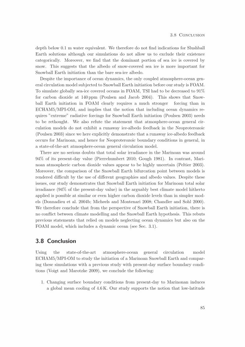
3.8 Conclusion
depth below 0.1 m water equivalent. We therefore do not find indications for Slushball
Earth solutions although our simulations do not allow us to exclude their existence
categorically. Moreover, we find that the dominant portion of sea ice is covered by
snow. This suggests that the albedo of snow-covered sea ice is more important for
Snowball Earth initiation than the bare sea-ice albedo.
Despite the importance of ocean dynamics, the only coupled atmosphere-ocean gen-
eral circulation model subjected to Snowball Earth initiation before our study is FOAM.
To simulate globally sea-ice covered oceans in FOAM, TSI had to be decreased to 91%
for carbon dioxide at 140 ppm (Poulsen and Jacob 2004). This shows that Snow-
ball Earth initiation in FOAM clearly requires a much stronger forcing than in
ECHAM5/MPI-OM, and implies that the notion that including ocean dynamics re-
quires ”extreme” radiative forcings for Snowball Earth initiation (Poulsen 2003) needs
to be rethought. We also refute the statement that atmosphere-ocean general cir-
culation models do not exhibit a runaway ice-albedo feedback in the Neoproterozoic
(Poulsen 2003) since we here explicitly demonstrate that a runaway ice-albedo feedback
occurs for Marinoan, and hence for Neoproterozoic boundary conditions in general, in
a state-of-the-art atmosphere-ocean general circulation model.
There are no serious doubts that total solar irradiance in the Marinoan was around
94% of its present-day value (Pierrehumbert 2010; Gough 1981). In contrast, Mari-
noan atmospheric carbon dioxide values appear to be highly uncertain (Peltier 2003).
Moreover, the comparison of the Snowball Earth bifurcation point between models is
rendered difficult by the use of different geographies and albedo values. Despite these
issues, our study demonstrates that Snowball Earth initiation for Marinoan total solar
irradiance (94% of the present-day value) in the arguably best climate model hitherto
applied is possible at similar or even higher carbon dioxide levels than in simpler mod-
els (Donnadieu et al. 2004b; Micheels and Montenari 2008; Chandler and Sohl 2000).
We therefore conclude that from the perspective of Snowball Earth initiation, there is
no conflict between climate modelling and the Snowball Earth hypothesis. This rebuts
previous statements that relied on models neglecting ocean dynamics but also on the
FOAM model, which includes a dynamic ocean (see Sec. 3.1).
3.8 Conclusion
Using the state-of-the-art atmosphere-ocean general circulation model
ECHAM5/MPI-OM to study the initiation of a Marinoan Snowball Earth and compar-
ing these simulations with a previous study with present-day surface boundary condi-
tions (Voigt and Marotzke 2009), we conclude the following:
1. Changing surface boundary conditions from present-day to Marinonan induces
a global mean cooling of 4.6 K. Our study supports the notion that low-latitude
85
Chapter 3 Initiation of a Marinoan Snowball Earth
continents facilitate Snowball Earth initiation, in contrast to a previous study
with the atmosphere-ocean general circulation model FOAM.
2. For pre-industrial atmospheric carbon dioxide, the Snowball Earth bifurcation
points is between 95.5 and 96% of the present-day value of total solar irradiance.
For total solar irradiance set to its Marinoan value, i.e., 94% of the present-day
total solar irradiance, a Snowball Earth is prevented by quadrupling atmospheric
carbon with respect to its pre-industrial concentration. We rebut previous con-
clusions that Snowball Earth initiation would require ”extreme” forcings.
3. The Marinoan Snowball Earth bifurcation point in terms of total solar irradiance
can be predicted by a zero-dimensional energy balance given the equilibrium mean
ocean potential temperature for the present-day total solar irradiance.
4. Sea-ice cover of more than 55% of the ocean surface area is unstable, akin to
what was found for present-day surface boundary conditions. ECHAM5/MPI-OM
therefore does not exhibit states with near-complete sea-ice cover but open equa-
torial waters. This is in contrast to modelling studies that neglected ocean dy-
namics.
3.A Sensitivity to vertical mixing parameters of the ocean
model
In this study, we inadvertently apply smaller Pacanowski-Philander (PP) vertical vis-
cosity and diffusivity parameters than for the transition to a modern Snowball Earth
(Voigt and Marotzke 2009) and the pre-industrial control run PI (cf. Sect. 3.2). This
study uses 0.2·10−2 m2s−1 instead of the five times larger value 1.0·10−2 m2s−1 of Voigt
and Marotzke (2009) and PI. We stress that both choices are in the range of ”accepted”
values and that here is no physical reason to prefer one over the other. Also, the PP
vertical viscosity and diffusivity parameters must be distinguished from the vertical
viscosity and diffusivity that is actually applied in the model; for details on how the
PP vertical viscosity and diffusivity parameters enter, among others, the calculation of
vertical viscosity and diffusivity we refer to Marsland et al. (2003).
One might nevertheless suspect that this parameter change might vitiate our com-
parison of the Marinoan and pre-industrial control climates, MAR and PI, or our result
for the Snowball Earth bifurcation point and maximum stable sea-ice cover. That none
of this is the case is demonstrated by the following simulations (see Table 3.5).
For the Marinoan control climate, quintupling PP vertical viscosity and diffusivity
parameters (simulation MAR-PP5) does not affect sea-ice area and surface tempera-
ture; both quantities agree in MAR and MAR-PP5 within their interannual variabili-
ties. Mean ocean potential temperature is increased by less than 0.04 K in MAR-PP5.
86
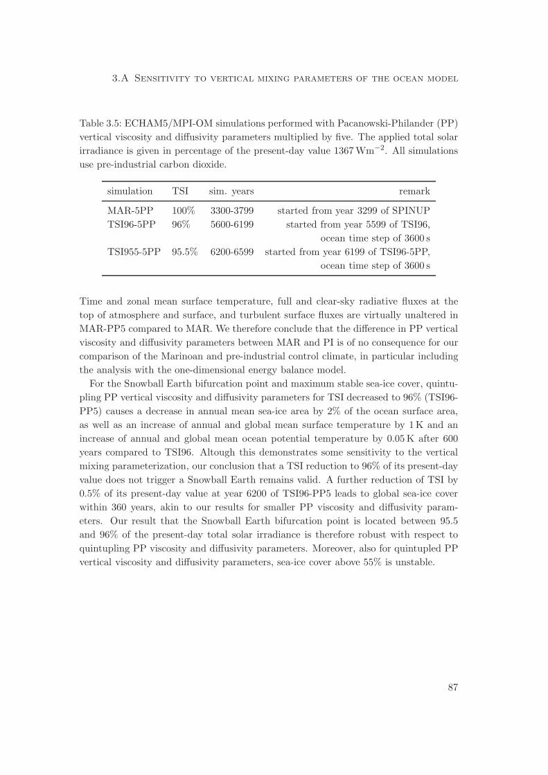
3.A Sensitivity to vertical mixing parameters of the ocean model
Table 3.5: ECHAM5/MPI-OM simulations performed with Pacanowski-Philander (PP)
vertical viscosity and diffusivity parameters multiplied by five. The applied total solar
irradiance is given in percentage of the present-day value 1367 Wm−2. All simulations
use pre-industrial carbon dioxide.
simulation TSI sim. years remark
MAR-5PP 100% 3300-3799 started from year 3299 of SPINUP
TSI96-5PP 96% 5600-6199 started from year 5599 of TSI96,
ocean time step of 3600 s
TSI955-5PP 95.5% 6200-6599 started from year 6199 of TSI96-5PP,
ocean time step of 3600 s
Time and zonal mean surface temperature, full and clear-sky radiative fluxes at the
top of atmosphere and surface, and turbulent surface fluxes are virtually unaltered in
MAR-PP5 compared to MAR. We therefore conclude that the difference in PP vertical
viscosity and diffusivity parameters between MAR and PI is of no consequence for our
comparison of the Marinoan and pre-industrial control climate, in particular including
the analysis with the one-dimensional energy balance model.
For the Snowball Earth bifurcation point and maximum stable sea-ice cover, quintu-
pling PP vertical viscosity and diffusivity parameters for TSI decreased to 96% (TSI96-
PP5) causes a decrease in annual mean sea-ice area by 2% of the ocean surface area,
as well as an increase of annual and global mean surface temperature by 1K and an
increase of annual and global mean ocean potential temperature by 0.05 K after 600
years compared to TSI96. Altough this demonstrates some sensitivity to the vertical
mixing parameterization, our conclusion that a TSI reduction to 96% of its present-day
value does not trigger a Snowball Earth remains valid. A further reduction of TSI by
0.5% of its present-day value at year 6200 of TSI96-PP5 leads to global sea-ice cover
within 360 years, akin to our results for smaller PP viscosity and diffusivity param-
eters. Our result that the Snowball Earth bifurcation point is located between 95.5
and 96% of the present-day total solar irradiance is therefore robust with respect to
quintupling PP viscosity and diffusivity parameters. Moreover, also for quintupled PP
vertical viscosity and diffusivity parameters, sea-ice cover above 55% is unstable.
87

Chapter 4
Equinox Hadley cell dynamics in a Snowball
Earth atmosphere
We use the state-of-the-art atmospheric general circulation model ECHAM5 to investi-
gate a cold and virtually dry Snowball Earth atmosphere that results from specifying sea
ice as the surface boundary condition everywhere, corresponding to a frozen aquaplanet,
while keeping total solar irradiance at its present-day value. The aim of this study is
the investigation of the meridional circulation of a Snowball Earth atmosphere, which,
due to missing moisture, might constitute an ideal though yet unexplored testbed for
theories of atmospheric dynamics. The meridional circulation consists of a thermally
direct cell extending from the equator to 45◦ N/S with ascent close to the equator, and
a weak thermally indirect cell with descent between 45 and 65◦ N/S and ascent near
the poles. The thermally direct cell is subdivided into a weak deep cell reaching well
into the stratosphere and a strong Hadley cell that is confined to the troposphere. The
dynamics of the Snowball Earth Hadley cell differ substantially from the dynamics of
the present-day Hadley cell. In the upper branch of the Snowball Earth Hadley cell,
mean meridional advection of mean absolute vorticity is not only balanced by eddy
momentum fluxes but also by vertical diffusion. Vertical diffusion also contributes to
the meridional momentum balance as it decelerates the Hadley cell by downgradient
momentum mixing between its upper and lower branches. Suppressing vertical mo-
mentum diffusion above 870 hPa results in an increase of the Hadley cell strength by a
factor of about 2, depending on the treatment of turbulent kinetic energy. Simulations
where we only suppress either vertical diffusion of zonal or meridional momentum show
that this increase can be understood from the decelerating effect of vertical diffusion
in the meridional momentum balance. Comparing our simulations with theories, we
conclude that neither axisymmetric Hadley cell models based on angular momentum
conservation nor eddy-permitting Hadley cell models that neglect vertical diffusion of
momentum are applicable to a Snowball Earth atmosphere under equinox insolation
since both assume an inviscid upper Hadley cell branch. Moreover, our results suggest
that dry atmospheres should not be considered as a-priori simpler testcases for Hadley
cell theories than moist atmospheres.
89
Chapter 4 Snowball Earth Hadley cell dynamics
4.1 Introduction
Developing a closed theory for the meridional circulation of the atmosphere remains
one of the main challenges in atmospheric dynamics. From the very beginning, a
particular focus has been laid on the Hadley cell, a synonym for the tropical overturning
circulation. In this study, we confront existing Hadley cell theories with a Snowball
Earth atmosphere simulated by a state-of-the-art atmosphere general circulation model,
and investigate if the assumptions made to derive these theories and hence the theories
themselves hold in this cold and virtually dry climate. To ease comparison with theories,
insolation follows equinox conditions with disabled diurnal cycle.
The challenge of atmospheric dynamics, in contrast to most natural science disci-
plines, is not in ascertaining the underlying dynamical equations. These are essentially
known. The art is in fact to distill, for a given problem, the primal terms of this cou-
pled set of non-linear and multi-scale partial differential equations, and to neglect the
others. One of the most prominent examples for this approach of theory building is the
Hadley circulation (see Lorenz (1967) for a historic review, and Schneider (2006) for a
summary of recent progress).
One important branch of Hadley cell theories, pioneered by Schneider (1977) and
Held and Hou (1980) and recently extended by Caballero et al. (2008), has emerged
from the postulate that the upper Hadley cell branch conserves angular momentum.
This assumption, combined with thermal wind balance and the requirement that no
energy is exported from the Hadley cell region, allows one to derive a closed Hadley
cell theory that predicts Hadley cell strength and width in dependence of only external
parameters like rotation rate and radiative-equilibrium pole-to-equator temperature
contrast (e.g., Held 2000).
One criticism of these models is that they produce too strong subtropical jets. The
latter is, at least partly, a consequence of neglecting non-axisymmetric motions, i.e. ed-
dies, and their momentum transport. As eddy effects were found to be non-negligible
in the upper Hadley cell branch of today’s atmosphere on Earth (Walker and Schneider
2006), one needs to account for them. Including their influence by dropping the ax-
isymmetric assumption leads to the second important branch of Hadley cell theories as
described in Schneider (2006). These theories do not posses the neat feature of being
analytically solvable since eddy momentum fluxes are a-priori unknown and depend on
the mean circulation, but simulations with idealized general circulation models allow
to derive scaling laws for the Hadley cell strength and width (Walker and Schneider
2006; Korty and Schneider 2008).
Despite large progress made in understanding Hadley cell dynamics (see Schneider
(2006) for a review), an investigation of the Hadley cell of a Snowball Earth atmosphere
is missing. The latter might constitute an ideal testbed for atmospheric dynamics be-
cause the near absence of water eliminates the hitherto unsolved problems of incorpo-
90
4.2 Model and simulation setup
rating the effect of latent heat and moist convection into a moist Hadley cell theory.
By offering a distinct realization of a dry atmosphere, the Snowball Earth therefore
should allow us to test the much further developed dry Hadley cell theories.
Taking a first step towards closing this gap, we apply the state-of-the-art atmosphere
general circulation model ECHAM5 (Roeckner et al. 2003). ECHAM5’s comprehen-
sive suite of physical parameterizations, including a full radiation code and dry con-
vection scheme, represents a major difference between our work and previous studies
(Walker and Schneider 2006; Korty and Schneider 2008) with an idealized general cir-
culation model. The latter model resolves the three-dimensional large-scale flow but
only crudely accounts for subgrid-scale processes. In particular, turbulent momentum
mixing, modelled by vertical diffusion, is restricted to the lowest part of the atmosphere
(see Schneider and Walker (2006) for details of this model).
This study investigates the dynamics of a Snowball Earth Hadley cell by analyzing the
zonal and meridional momentum balances. We do not focus on how the atmospheric
circulation might ease or hinder the deglaciation of a Snowball Earth. However, we
will be able to assess the importance of Hadley cell strength on equatorial surface
temperature.
The paper is organized as follows. Section 2 describes the atmosphere general circula-
tion model ECHAM5 and setup of the simulations. Section 3 summarizes main features
of the meridional circulation of a Snowball Earth atmosphere before a detailed analysis
of the zonal and meridional momentum balance is given in Sect. 4. Section 5 discusses
the effect of vertical diffusion on the Hadley cell strength and presents corresponding
simulations. In Section 6, we investigate the sensitivity of our results to the diurnal
cycle in insolation and to the model’s formulation of vertical diffusion. Section 7 gives
a general discussion of the results, section 8 follows with conclusions.
4.2 Model and simulation setup
We use the Max Planck Institute for Meteorology atmosphere general circulation model
ECHAM5.4.01 (labelled ECHAM5 in the following). ECHAM5 (Roeckner et al. 2003)
is the fifth generation of the ECHAM model series that originally evolved from the
weather prediction model of the European Centre for Medium Range Weather Fore-
casts. The dynamical core of ECHAM5 employs the spectral transform method with
triangular truncation to numerically solve the hydrostatic primitive equations of the
atmosphere. The prognostic variables are vorticity, divergence, temperature, and log-
arithm of surface pressure. A semi-implicit leapfrog scheme is used for time integra-
tion, with the growth of spurious computational modes inhibited by an Asselin filter.
ECHAM5 contains state-of-the-art physics parameterizations that are solved in grid-
point space on a Gaussian grid. The radiation scheme comprises 6 spectral bands for
shortwave radiation and 16 bands for longwave radiation, the latter is calculated by the
91
Chapter 4 Snowball Earth Hadley cell dynamics
Rapid Radiative Transfer Model (Mlawer et al. 1997). ECHAM5 contains a full turbu-
lence, or dry convection, scheme. Turbulent surface fluxes of momentum and heat are
calculated from a bulk aerodynamic formula. Transfer coefficients are obtained from
Monin-Obukhov similarity theory and depend on stability through the bulk Richard-
son number. Above the surface layer, vertical turbulent fluxes follow the eddy diffusion
method. Eddy viscosity and diffusivity depend on mixing length, Richardson num-
ber and turbulent kinetic energy (TKE). The dependence on Richardson number is
implemented via stability functions similar to Louis (1979). TKE is calculated by a
simplified prognostic TKE equation that neglects advection of TKE by the resolved
flow and uses eddy viscosity for all turbulent fluxes (Roeckner et al. 2003; Brinkop and
Roeckner 1995). The top of the boundary layer is diagnosed as the maximum of two
heights; one based on the friction velocity, the other defined as the highest level with
smaller dry static energy than the surface level.
ECHAM5 also contains parameterizations for stratiform clouds and cumulus convec-
tion (Tiedtke 1989; Nordeng 1994). These are only of little importance for the cold
and virtually dry Snowball Earth atmosphere investigated in this study. Similarly, the
scheme for gravity wave drag due to subgrid scale orography does not act here because
of the flat sea-ice surface (see below).
ECHAM5 has been successfully evaluated against observations (Roeckner et al. 2006;
Wild and Roeckner 2006) and, coupled to the Max Planck Institute for Meteorology
ocean general circulation model MPI-OM (Marsland et al. 2003), was used for the
integrations for the fourth assessment report of the Intergovernmental Panel on Climate
Change (e.g., Brasseur and Roeckner 2005; Bengtsson et al. 2006; Landerer et al. 2007).
In this study, we use ECHAM5 with idealized Snowball Earth boundary conditions.
The surface is specified as sea ice everywhere, corresponding to a frozen aqua planet
(Neale and Hoskins 2000a,b). Sea-ice thickness is nominally set to 1010 m to effectively
eliminate the conductive heat flux through sea ice from the surface energy balance. Sea-
ice surface temperature is calculated by the balance of surface radiative and turbulent
fluxes and assuming a specific heat capacity that corresponds to a sea-ice thickness of
0.1 m. This implies a small thermal inertia of the surface. According to the sea-ice
surface, roughness length is set to 10−3 m. Total solar irradiance is set to its present-
day value of 1365 Wm−2. The only atmospheric greenhouse gas apart from prognostic
water vapor is CO2 at a concentration of 300 ppm. The atmospheric concentration of
all other radiatively active trace gases (CH4,N2O,CFCs) is set to zero, and ozone as
well as aerosols are not accounted for in the radiation code. Solar insolation follows
permanent equinox conditions resulting from a circular orbit with zero obliquity and
disabled diurnal cycle (see Fig. 4.1).
We employ the medium-resolution version of ECHAM5 with spectral truncation T63
in the horizontal and 31 unevenly spaced hybrid σ-levels. In a comparison to ERA-40
data, this resolution was found to be only slightly inferior to higher resolution versions
92
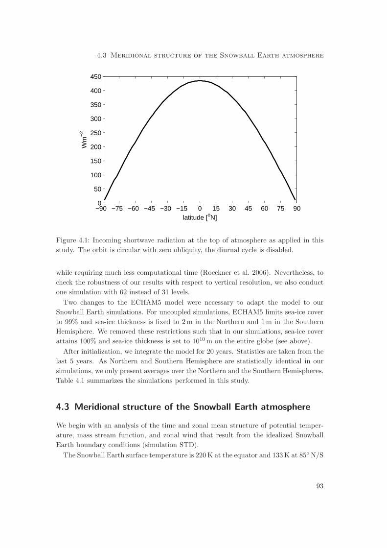
4.3 Meridional structure of the Snowball Earth atmosphere
−90 −75 −60 −45 −30 −15 0 15 30 45 60 75 900
50
100
150
200
250
300
350
400
450
latitude [oN]
Wm
−2
Figure 4.1: Incoming shortwave radiation at the top of atmosphere as applied in this
study. The orbit is circular with zero obliquity, the diurnal cycle is disabled.
while requiring much less computational time (Roeckner et al. 2006). Nevertheless, to
check the robustness of our results with respect to vertical resolution, we also conduct
one simulation with 62 instead of 31 levels.
Two changes to the ECHAM5 model were necessary to adapt the model to our
Snowball Earth simulations. For uncoupled simulations, ECHAM5 limits sea-ice cover
to 99% and sea-ice thickness is fixed to 2 m in the Northern and 1 m in the Southern
Hemisphere. We removed these restrictions such that in our simulations, sea-ice cover
attains 100% and sea-ice thickness is set to 1010 m on the entire globe (see above).
After initialization, we integrate the model for 20 years. Statistics are taken from the
last 5 years. As Northern and Southern Hemisphere are statistically identical in our
simulations, we only present averages over the Northern and the Southern Hemispheres.
Table 4.1 summarizes the simulations performed in this study.
4.3 Meridional structure of the Snowball Earth atmosphere
We begin with an analysis of the time and zonal mean structure of potential temper-
ature, mass stream function, and zonal wind that result from the idealized Snowball
Earth boundary conditions (simulation STD).
The Snowball Earth surface temperature is 220 K at the equator and 133 K at 85◦ N/S
93
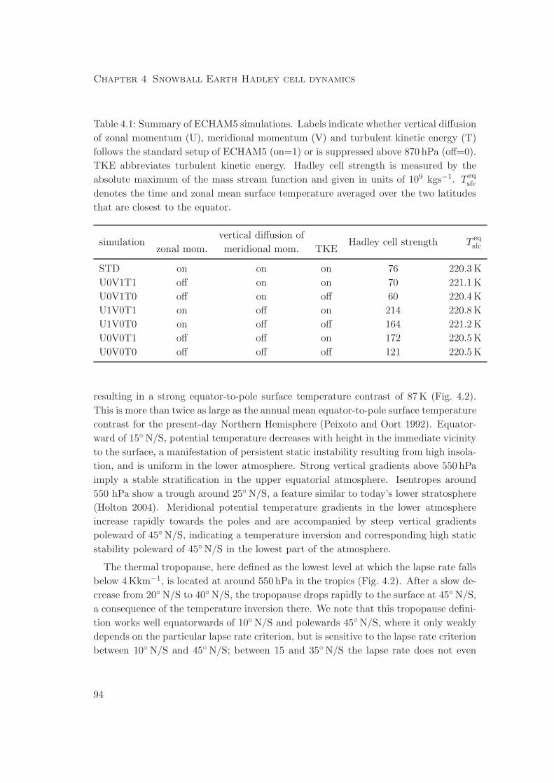
Chapter 4 Snowball Earth Hadley cell dynamics
Table 4.1: Summary of ECHAM5 simulations. Labels indicate whether vertical diffusion
of zonal momentum (U), meridional momentum (V) and turbulent kinetic energy (T)
follows the standard setup of ECHAM5 (on=1) or is suppressed above 870 hPa (off=0).
TKE abbreviates turbulent kinetic energy. Hadley cell strength is measured by the
absolute maximum of the mass stream function and given in units of 109 kgs−1. T eqsfc
denotes the time and zonal mean surface temperature averaged over the two latitudes
that are closest to the equator.
simulationvertical diffusion of
Hadley cell strength T eqsfczonal mom. meridional mom. TKE
STD on on on 76 220.3 K
U0V1T1 off on on 70 221.1 K
U0V1T0 off on off 60 220.4 K
U1V0T1 on off on 214 220.8 K
U1V0T0 on off off 164 221.2 K
U0V0T1 off off on 172 220.5 K
U0V0T0 off off off 121 220.5 K
resulting in a strong equator-to-pole surface temperature contrast of 87 K (Fig. 4.2).
This is more than twice as large as the annual mean equator-to-pole surface temperature
contrast for the present-day Northern Hemisphere (Peixoto and Oort 1992). Equator-
ward of 15◦ N/S, potential temperature decreases with height in the immediate vicinity
to the surface, a manifestation of persistent static instability resulting from high insola-
tion, and is uniform in the lower atmosphere. Strong vertical gradients above 550 hPa
imply a stable stratification in the upper equatorial atmosphere. Isentropes around
550 hPa show a trough around 25◦ N/S, a feature similar to today’s lower stratosphere
(Holton 2004). Meridional potential temperature gradients in the lower atmosphere
increase rapidly towards the poles and are accompanied by steep vertical gradients
poleward of 45◦ N/S, indicating a temperature inversion and corresponding high static
stability poleward of 45◦ N/S in the lowest part of the atmosphere.
The thermal tropopause, here defined as the lowest level at which the lapse rate falls
below 4 Kkm−1, is located at around 550 hPa in the tropics (Fig. 4.2). After a slow de-
crease from 20◦ N/S to 40◦ N/S, the tropopause drops rapidly to the surface at 45◦ N/S,
a consequence of the temperature inversion there. We note that this tropopause defini-
tion works well equatorwards of 10◦ N/S and polewards 45◦ N/S, where it only weakly
depends on the particular lapse rate criterion, but is sensitive to the lapse rate criterion
between 10◦ N/S and 45◦ N/S; between 15 and 35◦ N/S the lapse rate does not even
94
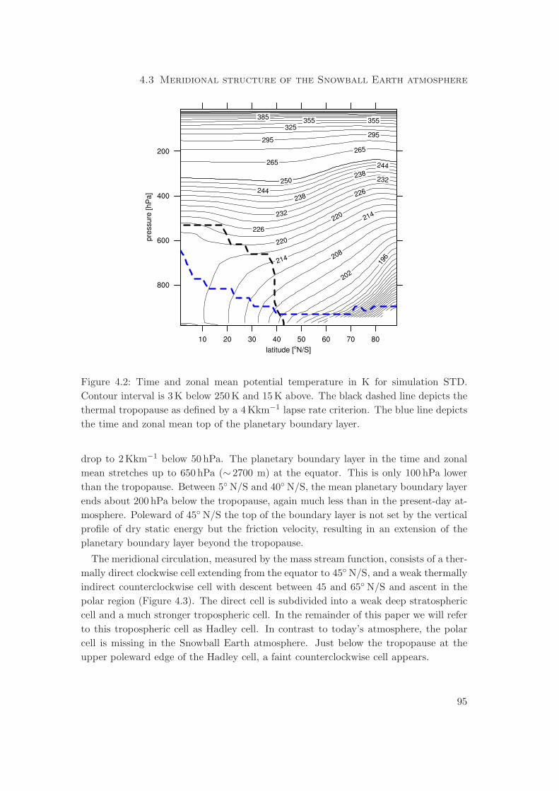
4.3 Meridional structure of the Snowball Earth atmosphere
Figure 4.2: Time and zonal mean potential temperature in K for simulation STD.
Contour interval is 3K below 250 K and 15 K above. The black dashed line depicts the
thermal tropopause as defined by a 4 Kkm−1 lapse rate criterion. The blue line depicts
the time and zonal mean top of the planetary boundary layer.
drop to 2Kkm−1 below 50 hPa. The planetary boundary layer in the time and zonal
mean stretches up to 650 hPa (∼ 2700 m) at the equator. This is only 100 hPa lower
than the tropopause. Between 5◦ N/S and 40◦ N/S, the mean planetary boundary layer
ends about 200 hPa below the tropopause, again much less than in the present-day at-
mosphere. Poleward of 45◦ N/S the top of the boundary layer is not set by the vertical
profile of dry static energy but the friction velocity, resulting in an extension of the
planetary boundary layer beyond the tropopause.
The meridional circulation, measured by the mass stream function, consists of a ther-
mally direct clockwise cell extending from the equator to 45◦ N/S, and a weak thermally
indirect counterclockwise cell with descent between 45 and 65◦ N/S and ascent in the
polar region (Figure 4.3). The direct cell is subdivided into a weak deep stratospheric
cell and a much stronger tropospheric cell. In the remainder of this paper we will refer
to this tropospheric cell as Hadley cell. In contrast to today’s atmosphere, the polar
cell is missing in the Snowball Earth atmosphere. Just below the tropopause at the
upper poleward edge of the Hadley cell, a faint counterclockwise cell appears.
95
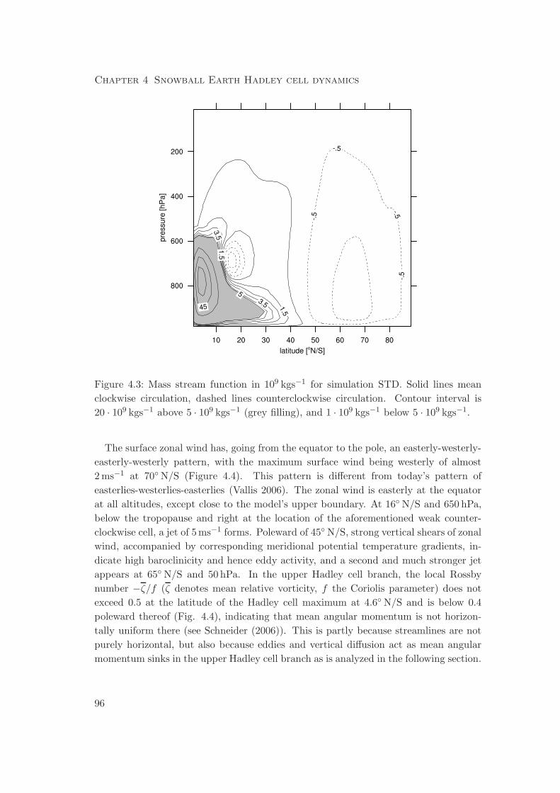
Chapter 4 Snowball Earth Hadley cell dynamics
Figure 4.3: Mass stream function in 109 kgs−1 for simulation STD. Solid lines mean
clockwise circulation, dashed lines counterclockwise circulation. Contour interval is
20 · 109 kgs−1 above 5 · 109 kgs−1 (grey filling), and 1 · 109 kgs−1 below 5 · 109 kgs−1.
The surface zonal wind has, going from the equator to the pole, an easterly-westerly-
easterly-westerly pattern, with the maximum surface wind being westerly of almost
2 ms−1 at 70◦ N/S (Figure 4.4). This pattern is different from today’s pattern of
easterlies-westerlies-easterlies (Vallis 2006). The zonal wind is easterly at the equator
at all altitudes, except close to the model’s upper boundary. At 16◦ N/S and 650 hPa,
below the tropopause and right at the location of the aforementioned weak counter-
clockwise cell, a jet of 5ms−1 forms. Poleward of 45◦ N/S, strong vertical shears of zonal
wind, accompanied by corresponding meridional potential temperature gradients, in-
dicate high baroclinicity and hence eddy activity, and a second and much stronger jet
appears at 65◦ N/S and 50 hPa. In the upper Hadley cell branch, the local Rossby
number −ζ/f (ζ denotes mean relative vorticity, f the Coriolis parameter) does not
exceed 0.5 at the latitude of the Hadley cell maximum at 4.6◦ N/S and is below 0.4
poleward thereof (Fig. 4.4), indicating that mean angular momentum is not horizon-
tally uniform there (see Schneider (2006)). This is partly because streamlines are not
purely horizontal, but also because eddies and vertical diffusion act as mean angular
momentum sinks in the upper Hadley cell branch as is analyzed in the following section.
96
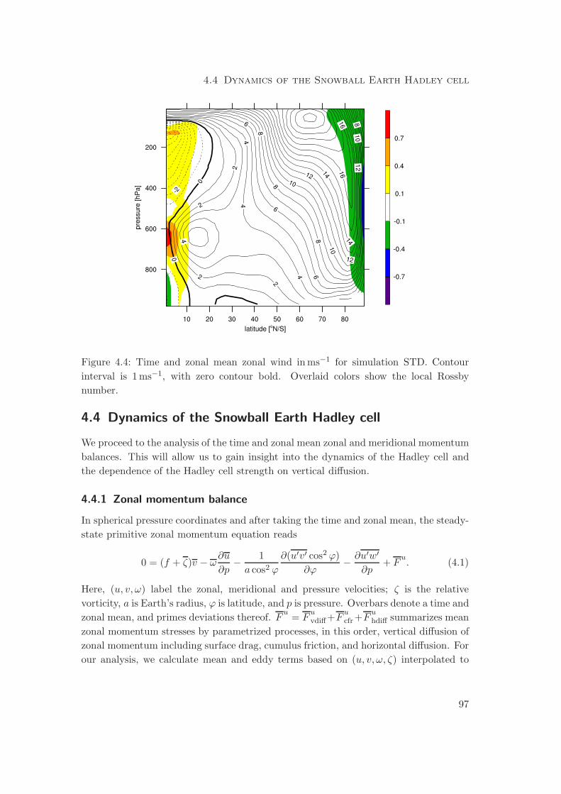
4.4 Dynamics of the Snowball Earth Hadley cell
Figure 4.4: Time and zonal mean zonal wind in ms−1 for simulation STD. Contour
interval is 1 ms−1, with zero contour bold. Overlaid colors show the local Rossby
number.
4.4 Dynamics of the Snowball Earth Hadley cell
We proceed to the analysis of the time and zonal mean zonal and meridional momentum
balances. This will allow us to gain insight into the dynamics of the Hadley cell and
the dependence of the Hadley cell strength on vertical diffusion.
4.4.1 Zonal momentum balance
In spherical pressure coordinates and after taking the time and zonal mean, the steady-
state primitive zonal momentum equation reads
0 = (f + ζ)v − ω∂u
∂p− 1
a cos2 ϕ
∂(u′v′ cos2 ϕ)
∂ϕ− ∂u′w′
∂p+ F
u. (4.1)
Here, (u, v, ω) label the zonal, meridional and pressure velocities; ζ is the relative
vorticity, a is Earth’s radius, ϕ is latitude, and p is pressure. Overbars denote a time and
zonal mean, and primes deviations thereof. Fu
= Fuvdiff+F
ucfr+F
uhdiff summarizes mean
zonal momentum stresses by parametrized processes, in this order, vertical diffusion of
zonal momentum including surface drag, cumulus friction, and horizontal diffusion. For
our analysis, we calculate mean and eddy terms based on (u, v, ω, ζ) interpolated to
97
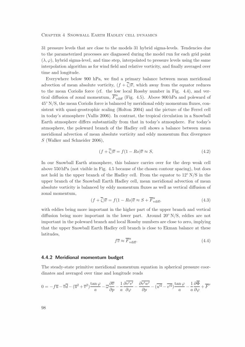
Chapter 4 Snowball Earth Hadley cell dynamics
31 pressure levels that are close to the models 31 hybrid sigma-levels. Tendencies due
to the parameterized processes are diagnosed during the model run for each grid point
(λ,ϕ), hybrid sigma-level, and time step, interpolated to pressure levels using the same
interpolation algorithm as for wind field and relative vorticity, and finally averaged over
time and longitude.
Everywhere below 900 hPa, we find a primary balance between mean meridional
advection of mean absolute vorticity, (f + ζ)v, which away from the equator reduces
to the mean Coriolis force (cf. the low local Rossby number in Fig. 4.4), and ver-
tical diffusion of zonal momentum, Fuvdiff (Fig. 4.5). Above 900 hPa and poleward of
45◦ N/S, the mean Coriolis force is balanced by meridional eddy momentum fluxes, con-
sistent with quasi-geostrophic scaling (Holton 2004) and the picture of the Ferrel cell
in today’s atmosphere (Vallis 2006). In contrast, the tropical circulation in a Snowball
Earth atmosphere differs substantially from that in today’s atmosphere. For today’s
atmosphere, the poleward branch of the Hadley cell shows a balance between mean
meridional advection of mean absolute vorticity and eddy momentum flux divergence
S (Walker and Schneider 2006),
(f + ζ)v = f(1 −Ro)v ≈ S, (4.2)
In our Snowball Earth atmosphere, this balance carries over for the deep weak cell
above 550 hPa (not visible in Fig. 4.5 because of the chosen contour spacing), but does
not hold in the upper branch of the Hadley cell. From the equator to 12◦ N/S in the
upper branch of the Snowball Earth Hadley cell, mean meridional advection of mean
absolute vorticity is balanced by eddy momentum fluxes as well as vertical diffusion of
zonal momentum,
(f + ζ)v = f(1 −Ro)v ≈ S + Fuvdiff, (4.3)
with eddies being more important in the higher part of the upper branch and vertical
diffusion being more important in the lower part. Around 20◦ N/S, eddies are not
important in the poleward branch and local Rossby numbers are close to zero, implying
that the upper Snowball Earth Hadley cell branch is close to Ekman balance at these
latitudes,
fv ≈ Fuvdiff. (4.4)
4.4.2 Meridional momentum budget
The steady-state primitive meridional momentum equation in spherical pressure coor-
dinates and averaged over time and longitude reads
0 = −fu− vd− (u2 + v2)tanϕ
a−ω∂v
∂p− 1
a
∂v′v′
∂ϕ− ∂v′w′
∂p− (u′2 − v′2)tanϕ
a− 1
a
∂Φ
∂ϕ+F
v
98
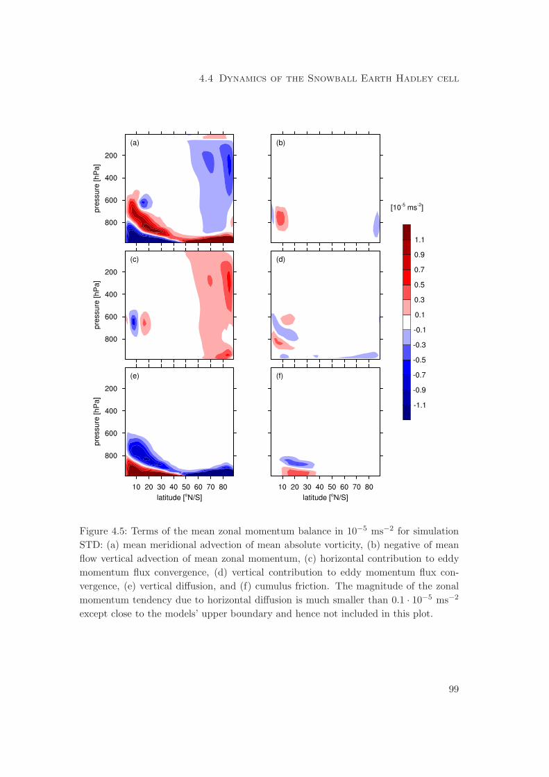
4.4 Dynamics of the Snowball Earth Hadley cell
Figure 4.5: Terms of the mean zonal momentum balance in 10−5 ms−2 for simulation
STD: (a) mean meridional advection of mean absolute vorticity, (b) negative of mean
flow vertical advection of mean zonal momentum, (c) horizontal contribution to eddy
momentum flux convergence, (d) vertical contribution to eddy momentum flux con-
vergence, (e) vertical diffusion, and (f) cumulus friction. The magnitude of the zonal
momentum tendency due to horizontal diffusion is much smaller than 0.1 · 10−5 ms−2
except close to the models’ upper boundary and hence not included in this plot.
99
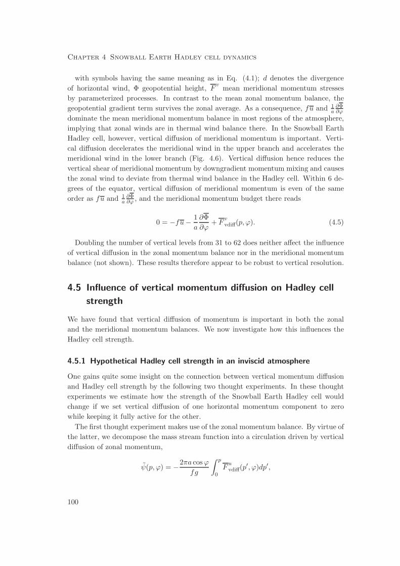
Chapter 4 Snowball Earth Hadley cell dynamics
with symbols having the same meaning as in Eq. (4.1); d denotes the divergence
of horizontal wind, Φ geopotential height, Fv
mean meridional momentum stresses
by parameterized processes. In contrast to the mean zonal momentum balance, the
geopotential gradient term survives the zonal average. As a consequence, fu and 1a
∂Φ∂ϕ
dominate the mean meridional momentum balance in most regions of the atmosphere,
implying that zonal winds are in thermal wind balance there. In the Snowball Earth
Hadley cell, however, vertical diffusion of meridional momentum is important. Verti-
cal diffusion decelerates the meridional wind in the upper branch and accelerates the
meridional wind in the lower branch (Fig. 4.6). Vertical diffusion hence reduces the
vertical shear of meridional momentum by downgradient momentum mixing and causes
the zonal wind to deviate from thermal wind balance in the Hadley cell. Within 6 de-
grees of the equator, vertical diffusion of meridional momentum is even of the same
order as fu and 1a
∂Φ∂ϕ , and the meridional momentum budget there reads
0 = −fu− 1
a
∂Φ
∂ϕ+ F
vvdiff(p, ϕ). (4.5)
Doubling the number of vertical levels from 31 to 62 does neither affect the influence
of vertical diffusion in the zonal momentum balance nor in the meridional momentum
balance (not shown). These results therefore appear to be robust to vertical resolution.
4.5 Influence of vertical momentum diffusion on Hadley cell
strength
We have found that vertical diffusion of momentum is important in both the zonal
and the meridional momentum balances. We now investigate how this influences the
Hadley cell strength.
4.5.1 Hypothetical Hadley cell strength in an inviscid atmosphere
One gains quite some insight on the connection between vertical momentum diffusion
and Hadley cell strength by the following two thought experiments. In these thought
experiments we estimate how the strength of the Snowball Earth Hadley cell would
change if we set vertical diffusion of one horizontal momentum component to zero
while keeping it fully active for the other.
The first thought experiment makes use of the zonal momentum balance. By virtue of
the latter, we decompose the mass stream function into a circulation driven by vertical
diffusion of zonal momentum,
ψ(p, ϕ) = −2πa cosϕ
fg
∫ p
0
Fuvdiff(p′, ϕ)dp′,
100
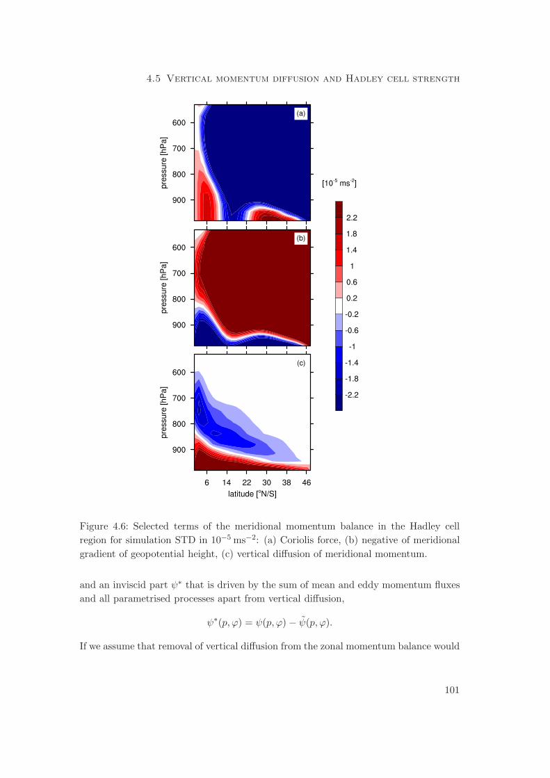
4.5 Vertical momentum diffusion and Hadley cell strength
Figure 4.6: Selected terms of the meridional momentum balance in the Hadley cell
region for simulation STD in 10−5 ms−2: (a) Coriolis force, (b) negative of meridional
gradient of geopotential height, (c) vertical diffusion of meridional momentum.
and an inviscid part ψ∗ that is driven by the sum of mean and eddy momentum fluxes
and all parametrised processes apart from vertical diffusion,
ψ∗(p, ϕ) = ψ(p, ϕ) − ψ(p, ϕ).
If we assume that removal of vertical diffusion from the zonal momentum balance would
101
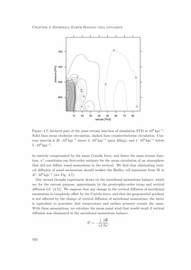
Chapter 4 Snowball Earth Hadley cell dynamics
Figure 4.7: Inviscid part of the mass stream function of simulation STD in 109 kgs−1.
Solid lines mean clockwise circulation, dashed lines counterclockwise circulation. Con-
tour interval is 20 · 109 kgs−1 above 5 · 109 kgs−1 (grey filling), and 1 · 109 kgs−1 below
5 · 109 kgs−1.
be entirely compensated by the mean Coriolis force, and hence the mass stream func-
tion, ψ∗ constitutes our first-order estimate for the mean circulation of an atmosphere
that did not diffuse zonal momentum in the vertical. We find that eliminating verti-
cal diffusion of zonal momentum should weaken the Hadley cell maximum from 76 to
47 · 109 kgs−1 (see Fig. 4.7).
Our second thought experiment draws on the meridional momentum balance, which
we, for the current purpose, approximate by the geostrophic-order terms and vertical
diffusion (cf. (4.5)). We suppose that any change in the vertical diffusion of meridional
momentum is completely offset by the Coriolis force, and that the geopotential gradient
is not affected by the change of vertical diffusion of meridional momentum; the latter
is equivalent to postulate that temperature and surface pressure remain the same.
With these assumptions, we calculate the mean zonal wind that would result if vertical
diffusion was eliminated in the meridional momentum balance,
u† = − 1
af
∂Φ
∂ϕ,
102
4.5 Vertical momentum diffusion and Hadley cell strength
and from this the corresponding mean relative vorticity (Vallis 2006),
ζ†
= − 1
a cosϕ
∂
∂ϕ
(
u† cosϕ)
=1
a2 cosϕ
∂
∂ϕ
(
cosϕ
f
∂Φ
∂ϕ
)
.
Replacing mean relative vorticity by ζ†
and demanding that the mean meridional ve-
locity will adapt such that the mean meridional advection of mean absolute vorticity
remains the same,
(f + ζ)v = (f + ζ†)v†, (4.6)
we arrive at our first-oder estimate for the mass stream function in an atmosphere free
of vertical diffusion of meridional momentum,
ψ†(p, ϕ) =2πa cosϕ
fg
∫ p
0
f + ζ
f + ζ†vdp′. (4.7)
At the Hadley cell maximum, the mass stream function is predicted to increase from
76 to 114 · 109 kgs−1. An increase in the Hadley cell strength when vertical diffusion of
meridional momentum is suppressed is consistent with the decelerating effect of vertical
diffusion on the Hadley cell.
Our thought experiments suggest that removing vertical diffusion of zonal momentum
should weaken the Hadley cell by the same amount as suppressing vertical diffusion of
meridional momentum should strengthen it. We now test both ideas in our state-of-
the-art atmospheric general circulation model.
4.5.2 Simulations with suppressed vertical diffusion of horizontal
momentum
We now report on simulations where we suppress vertical diffusion of horizontal mo-
mentum above 870 hPa. This is achieved by changing eddy viscosity in the following
way. Additional to the eddy viscosity Km computed by ECHAM5’s turbulence scheme,
we introduce a restricted eddy viscosity K′
m that equals Km for the lowest 4 model lev-
els (surface to ≃ 945 hPa) and is set to 10−8m2s−1 above model level 26 (≃ 870 hPa).
At model level 27 (≃ 910 hPa), we set K′
m = 0.5 ·Km for a somewhat smoother shape
of the restricted eddy viscosity. If we apply K′
m instead of Km, we effectively suppress
vertical momentum diffusion above 870 hPa and hence restrict it to the lowest part of
the atmosphere.
This approach allows us to test the effect of individually suppressing vertical diffusion
of either zonal or meridional momentum by applying the restricted eddy viscosity K′
m to
one of the horizontal momentum components while applying the full eddy viscosity Km
to the other component. Implementing this approach is straightforward but introduces
a potentially important ambiguity in the treatment of turbulent kinetic energy (TKE).
103
Chapter 4 Snowball Earth Hadley cell dynamics
Recall that eddy viscosity depends on the square root of TKE, and that TKE itself
is calculated by a simplified prognostic TKE equation that neglects horizontal TKE
advection (Roeckner et al. 2003). The numerical technique to solve the TKE equation
involves vertical TKE diffusion with eddy viscosity used as diffusion coefficient (Brinkop
and Roeckner 1995). Altering vertical diffusion of horizontal momentum therefore also
requires to decide whether we apply the full or restricted eddy viscosity for vertical TKE
diffusion. We stress that the eddy diffusivity used for the vertical diffusion of dry static
energy is not changed by this procedure in any part of the atmosphere. Changes in
the flow and temperature field resulting from suppressing vertical momentum diffusion
may lead to changes in eddy diffusivity and viscosity compared to STD, however.
In total, we perform six simulations spanning the six combinations of choosing full or
restricted eddy viscosity for zonal momentum, meridional momentum, and turbulent
kinetic energy (Table 4.1).
In line with the results of our thought experiments, suppressing vertical diffusion of
zonal momentum weakens the Hadley cell while suppressing vertical diffusion of merid-
ional momentum strengthens it (Figure 4.8 and Table 4.1). The exact magnitudes differ
from our first-order estimates, however. Suppressing vertical diffusion of zonal momen-
tum only moderately reduces the Hadley cell strength to 60 to 70 ·109 kgs−1, depending
on vertical TKE diffusion (simulations U0V1T0 and U0V1T1). In contrast, suppressing
vertical diffusion of meridional momentum strongly increases the Hadley cell to 164 to
214 ·109 kgs−1 (simulations U1V0T0 and U1V0T1). This is much higher than our esti-
mate. The increase of Hadley cell strength resulting from suppressing vertical diffusion
of both horizontal momentum components is similar to the average of the individual
responses (U0V0T0 and U0V0T1). Simulations with full TKE diffusion have stronger
Hadley cells than their counterparts with suppressed TKE diffusion, showing that the
treatment of vertical TKE diffusion systemattically influences the Hadley cell strength.
The same holds for the shape of the Hadley cell. For example, the Hadley cell extends
higher up for full TKE diffusion. Moreover, the weak counterclockwise cell at 15◦ N/S
extends closer to the surface when suppressed vertical diffusion of zonal momentum
meets suppressed (U0V1T0,U0V0T0) instead of full (U0V1T1,U0V0T1) vertical TKE
diffusion.
Despite the influence of the treatment of TKE on the exact Hadley cell strength, we
find a robust response of the Hadley cell strength. Suppressing vertical diffusion of zonal
momentum moderately weakens the Hadley cell while suppressing vertical diffusion of
meridional momentum strongly strengthens the Hadley cell. The zonal momentum
balance that results from suppressing vertical diffusion of zonal and meridional mo-
mentum exhibits two features that are worth noting (Fig. 4.9). First, horizontal eddies
now converge zonal momentum to the equator, which is associated with weak equatorial
superrotation between 530 and 750 hPa. Second, vertical eddies become much stronger
and compensate, at least partly, for the loss of vertical diffusion of zonal momentum.
104
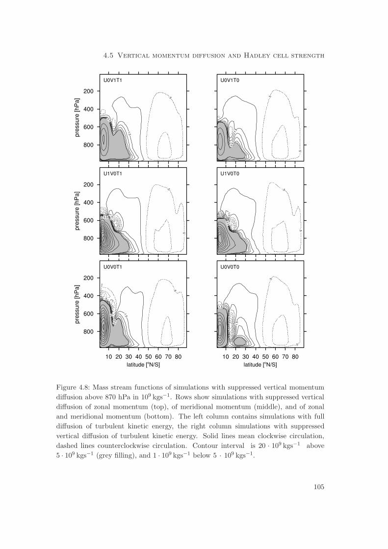
4.5 Vertical momentum diffusion and Hadley cell strength
Figure 4.8: Mass stream functions of simulations with suppressed vertical momentum
diffusion above 870 hPa in 109 kgs−1. Rows show simulations with suppressed vertical
diffusion of zonal momentum (top), of meridional momentum (middle), and of zonal
and meridional momentum (bottom). The left column contains simulations with full
diffusion of turbulent kinetic energy, the right column simulations with suppressed
vertical diffusion of turbulent kinetic energy. Solid lines mean clockwise circulation,
dashed lines counterclockwise circulation. Contour interval is 20 · 109 kgs−1 above
5 · 109 kgs−1 (grey filling), and 1 · 109 kgs−1 below 5 · 109 kgs−1.
105
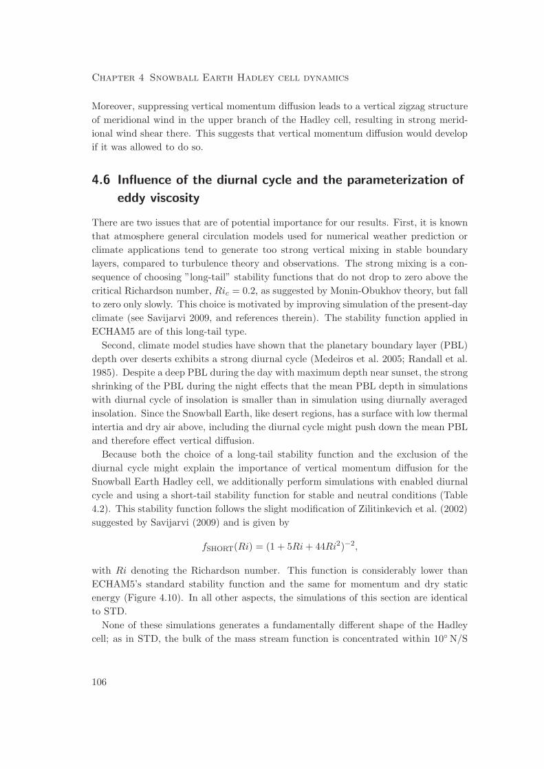
Chapter 4 Snowball Earth Hadley cell dynamics
Moreover, suppressing vertical momentum diffusion leads to a vertical zigzag structure
of meridional wind in the upper branch of the Hadley cell, resulting in strong merid-
ional wind shear there. This suggests that vertical momentum diffusion would develop
if it was allowed to do so.
4.6 Influence of the diurnal cycle and the parameterization of
eddy viscosity
There are two issues that are of potential importance for our results. First, it is known
that atmosphere general circulation models used for numerical weather prediction or
climate applications tend to generate too strong vertical mixing in stable boundary
layers, compared to turbulence theory and observations. The strong mixing is a con-
sequence of choosing ”long-tail” stability functions that do not drop to zero above the
critical Richardson number, Ric = 0.2, as suggested by Monin-Obukhov theory, but fall
to zero only slowly. This choice is motivated by improving simulation of the present-day
climate (see Savijarvi 2009, and references therein). The stability function applied in
ECHAM5 are of this long-tail type.
Second, climate model studies have shown that the planetary boundary layer (PBL)
depth over deserts exhibits a strong diurnal cycle (Medeiros et al. 2005; Randall et al.
1985). Despite a deep PBL during the day with maximum depth near sunset, the strong
shrinking of the PBL during the night effects that the mean PBL depth in simulations
with diurnal cycle of insolation is smaller than in simulation using diurnally averaged
insolation. Since the Snowball Earth, like desert regions, has a surface with low thermal
intertia and dry air above, including the diurnal cycle might push down the mean PBL
and therefore effect vertical diffusion.
Because both the choice of a long-tail stability function and the exclusion of the
diurnal cycle might explain the importance of vertical momentum diffusion for the
Snowball Earth Hadley cell, we additionally perform simulations with enabled diurnal
cycle and using a short-tail stability function for stable and neutral conditions (Table
4.2). This stability function follows the slight modification of Zilitinkevich et al. (2002)
suggested by Savijarvi (2009) and is given by
fSHORT(Ri) = (1 + 5Ri+ 44Ri2)−2,
with Ri denoting the Richardson number. This function is considerably lower than
ECHAM5’s standard stability function and the same for momentum and dry static
energy (Figure 4.10). In all other aspects, the simulations of this section are identical
to STD.
None of these simulations generates a fundamentally different shape of the Hadley
cell; as in STD, the bulk of the mass stream function is concentrated within 10◦ N/S
106
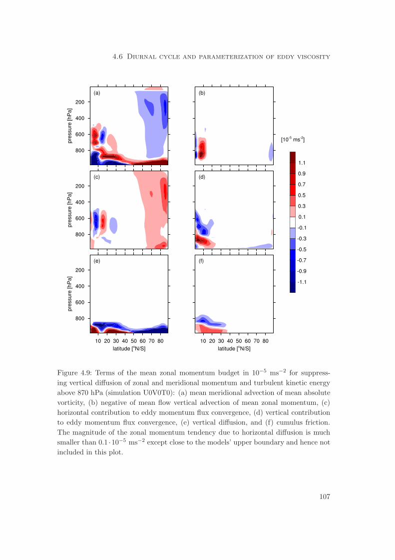
4.6 Diurnal cycle and parameterization of eddy viscosity
Figure 4.9: Terms of the mean zonal momentum budget in 10−5 ms−2 for suppress-
ing vertical diffusion of zonal and meridional momentum and turbulent kinetic energy
above 870 hPa (simulation U0V0T0): (a) mean meridional advection of mean absolute
vorticity, (b) negative of mean flow vertical advection of mean zonal momentum, (c)
horizontal contribution to eddy momentum flux convergence, (d) vertical contribution
to eddy momentum flux convergence, (e) vertical diffusion, and (f) cumulus friction.
The magnitude of the zonal momentum tendency due to horizontal diffusion is much
smaller than 0.1 ·10−5 ms−2 except close to the models’ upper boundary and hence not
included in this plot.
107
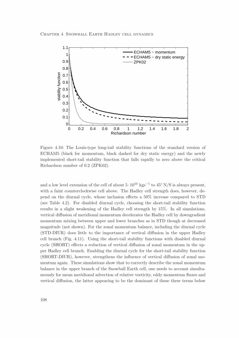
Chapter 4 Snowball Earth Hadley cell dynamics
0 0.2 0.4 0.6 0.8 1 1.2 1.4 1.6 1.8 20
0.1
0.2
0.3
0.4
0.5
0.6
0.7
0.8
0.9
1
1.1
Richardson number
stab
ility
func
tion
ECHAM5 − momentumECHAM5 − dry static energyZPK02
Figure 4.10: The Louis-type long-tail stability functions of the standard version of
ECHAM5 (black for momentum, black dashed for dry static energy) and the newly
implemented short-tail stability function that falls rapidly to zero above the critical
Richardson number of 0.2 (ZPK02).
and a low level extension of the cell of about 5 ·1010 kgs−1 to 45◦ N/S is always present,
with a faint counterclockwise cell above. The Hadley cell strength does, however, de-
pend on the diurnal cycle, whose inclusion effects a 50% increase compared to STD
(see Table 4.2). For disabled diurnal cycle, choosing the short-tail stability function
results in a slight weakening of the Hadley cell strength by 15%. In all simulations,
vertical diffusion of meridional momentum decelerates the Hadley cell by downgradient
momentum mixing between upper and lower branches as in STD though at decreased
magnitude (not shown). For the zonal momentum balance, including the diurnal cycle
(STD-DIUR) does little to the importance of vertical diffusion in the upper Hadley
cell branch (Fig. 4.11). Using the short-tail stability functions with disabled diurnal
cycle (SHORT) effects a reduction of vertical diffusion of zonal momentum in the up-
per Hadley cell branch. Enabling the diurnal cycle for the short-tail stability function
(SHORT-DIUR), however, strengthens the influence of vertical diffusion of zonal mo-
mentum again. These simulations show that to correctly describe the zonal momentum
balance in the upper branch of the Snowball Earth cell, one needs to account simulta-
neously for mean meridional advection of relative vorticity, eddy momentum fluxes and
vertical diffusion, the latter appearing to be the dominant of these three terms below
108
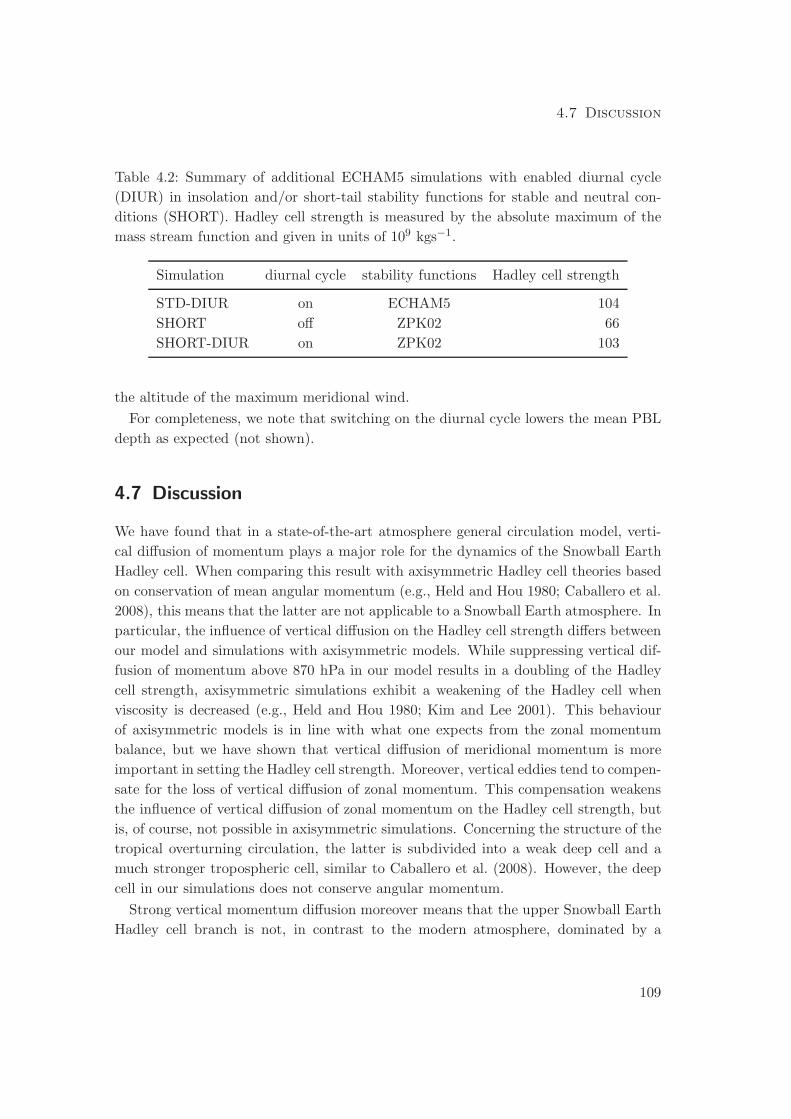
4.7 Discussion
Table 4.2: Summary of additional ECHAM5 simulations with enabled diurnal cycle
(DIUR) in insolation and/or short-tail stability functions for stable and neutral con-
ditions (SHORT). Hadley cell strength is measured by the absolute maximum of the
mass stream function and given in units of 109 kgs−1.
Simulation diurnal cycle stability functions Hadley cell strength
STD-DIUR on ECHAM5 104
SHORT off ZPK02 66
SHORT-DIUR on ZPK02 103
the altitude of the maximum meridional wind.
For completeness, we note that switching on the diurnal cycle lowers the mean PBL
depth as expected (not shown).
4.7 Discussion
We have found that in a state-of-the-art atmosphere general circulation model, verti-
cal diffusion of momentum plays a major role for the dynamics of the Snowball Earth
Hadley cell. When comparing this result with axisymmetric Hadley cell theories based
on conservation of mean angular momentum (e.g., Held and Hou 1980; Caballero et al.
2008), this means that the latter are not applicable to a Snowball Earth atmosphere. In
particular, the influence of vertical diffusion on the Hadley cell strength differs between
our model and simulations with axisymmetric models. While suppressing vertical dif-
fusion of momentum above 870 hPa in our model results in a doubling of the Hadley
cell strength, axisymmetric simulations exhibit a weakening of the Hadley cell when
viscosity is decreased (e.g., Held and Hou 1980; Kim and Lee 2001). This behaviour
of axisymmetric models is in line with what one expects from the zonal momentum
balance, but we have shown that vertical diffusion of meridional momentum is more
important in setting the Hadley cell strength. Moreover, vertical eddies tend to compen-
sate for the loss of vertical diffusion of zonal momentum. This compensation weakens
the influence of vertical diffusion of zonal momentum on the Hadley cell strength, but
is, of course, not possible in axisymmetric simulations. Concerning the structure of the
tropical overturning circulation, the latter is subdivided into a weak deep cell and a
much stronger tropospheric cell, similar to Caballero et al. (2008). However, the deep
cell in our simulations does not conserve angular momentum.
Strong vertical momentum diffusion moreover means that the upper Snowball Earth
Hadley cell branch is not, in contrast to the modern atmosphere, dominated by a
109
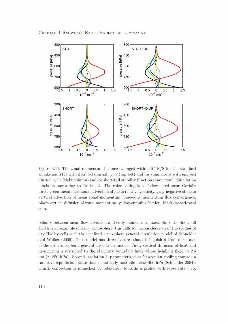
Chapter 4 Snowball Earth Hadley cell dynamics
−1.5 −1 −0.5 0 0.5 1 1.5
300
450
600
750
900
STD
10−5 ms−2
pres
sure
[hP
a]
−1.5 −1 −0.5 0 0.5 1 1.5
300
450
600
750
900
STD−DIUR
10−5 ms−2
pres
sure
[hP
a]
−1.5 −1 −0.5 0 0.5 1 1.5
300
450
600
750
900
SHORT
10−5 ms−2
pres
sure
[hP
a]
−1.5 −1 −0.5 0 0.5 1 1.5
300
450
600
750
900
SHORT−DIUR
10−5 ms−2
pres
sure
[hP
a]
Figure 4.11: The zonal momentum balance averaged within 10◦ N/S for the standard
simulation STD with disabled diurnal cycle (top left) and for simulations with enabled
diurnal cycle (right column) and/or short-tail stability function (lower row). Simulation
labels are according to Table 4.2. The color coding is as follows: red-mean Coriolis
force, green-mean meridional advection of mean relative vorticity, gray-negative of mean
vertical advection of mean zonal momentum, blue-eddy momentum flux convergence,
black-vertical diffusion of zonal momentum, yellow-cumulus friction, black dashed-total
sum.
balance between mean flow advection and eddy momentum fluxes. Since the Snowball
Earth is an example of a dry atmosphere, this calls for reconsideration of the studies of
dry Hadley cells with the idealized atmosphere general circulation model of Schneider
and Walker (2006). This model has three features that distinguish it from our state-
of-the-art atmospheric general circulation model. First, vertical diffusion of heat and
momentum is restricted to the planetary boundary layer whose height is fixed to 2.5
km (≃ 850 hPa). Second, radiation is parameterized as Newtonian cooling towards a
radiative equilibrium state that is statically unstable below 400 hPa (Schneider 2004).
Third, convection is mimicked by relaxation towards a profile with lapse rate γ Γd,
110
4.7 Discussion
where Γd denotes the dry adiabatic lapse rate (Walker and Schneider 2006). In the dry
case γ = 1 relevant for Snowball Earth, the statically unstable radiative temperature
profile suggests that dry convection in this model is active up to 400 hPa, but that it
has no influence on momentum above 850 hPa. This is in fundamental contrast to our
model, in which dry convection, modelled by vertical diffusion, acts on temperature
and momentum. In the light of the importance of vertical diffusion on the Snowball
Earth Hadley cell, the exclusion of convective momentum mixing in the idealized model
appears too strong a simplification. This simplification does have a large effect on
the Hadley cell strength and shape as shown by our simulations. The Hadley cell
strength increases by about a factor of 2 when we suppress vertical diffusion of zonal
and meridional momentum above 870 hPa but allow for vertical diffusion of dry static
energy, similar to how dry convection works in the idealized model. In total, this casts
doubts on the scaling laws for dry Hadley cells predicted by such an idealized model
(Walker and Schneider 2006). We also note that observations of today’s atmosphere
have shown that the planetary boundary layer can reach several kilometers over deserts,
leading to strong dry convection there (Gamo 1996).
The Snowball Earth atmosphere is very different from today’s atmosphere because
of its low temperatures and near-zero moisture content. This has two consequences.
First, tropopause and boundary layer are maximally separated by 250 hPa in a Snow-
ball Earth atmosphere and are hence much closer than today. The low tropopause
is consistent with the low surface temperatures, while the comparably high boundary
layer appears as a consequence of missing latent heat release. Second, the upper and
lower branches of the Snowball Earth Hadley cell are not separated by a region of
nearly vanishing meridional flow. This leads to strong meridional wind shear, making
meridional momentum transfer between upper and lower branches possible. Our re-
sults therefore do not imply that vertical momentum diffusion is also of importance in
today’s atmosphere.
In optically thin atmospheres that are nearly transparent to solar radiation, longwave
cooling destabilizes the troposphere (Pierrehumbert 2010). Because the effect of latent
heat release is missing in dry atmospheres, the necessary stabilization can be achieved
either by vertical diffusion or temperature advection. This implies that the intensity of
vertical diffusion is intimately connected to the influence of the circulation on temper-
ature. We have bypassed this issue here, but our results show that understanding the
dynamics of dry Hadley cells requires not only to consider the horizontal momentum
equation, but also the thermodynamic equation.
Our results have two important implications for building a Hadley cell theory. First,
the strengthening of the Hadley cell with enabled diurnal cycle makes clear that the
latter has to be included in the theory, at least in cases with low thermal inertia of
the surface. We do not know of any Hadley cell model that accounts for the diurnal
cycle. Second, the vital role of vertical diffusion for dry Hadley cells, requiring that dry
111
Chapter 4 Snowball Earth Hadley cell dynamics
convection and boundary layer dynamics must be taken into account, points out that
dry atmospheres in general should not be considered as a-priori simpler testcases for
Hadley cell theories than moist atmospheres. Idealized atmospheric general circulation
models that do not include momentum transfer by dry convection should not be viewed
as models for dry atmospheres but as models that highlight the interaction of mean
flow and eddies in the absence of subgrid-scale processes.
We have not analyzed the Snowball Earth Hadley cell extent in detail, partly because
defining the latter seems ambiguous given the shape of the Hadley cell. Moreover,
we have only studied equinox insolation. Repeating this study for solstice insolation
might reveal that vertical momentum diffusion is of less importance when the heating
is displaced from the equator, similar to what was found for the influence of eddies
(Walker and Schneider 2005, 2006).
Despite the large differences in Hadley cell strength and shape among our set of
simulations, equatorial surface temperature is close to 220 K in all simulations (Table
4.1). This suggests that the equatorial surface temperature is largely set by radiation
in our idealized Snowball Earth atmosphere, with virtually no influence of the Hadley
cell.
4.8 Conclusions
Using the state-of-the-art atmosphere general circulation model ECHAM5 to study
the tropical circulation of an idealized Snowball Earth atmosphere subject to equinox
insolation, we conclude the following� The upper branch of the equinox Snowball Earth Hadley cell is strongly influenced
by vertical momentum diffusion. This is in contrast to todays’s atmosphere.� Vertical diffusion of meridional momentum exhibits a stronger control on the
Snowball Earth Hadley cell than vertical diffusion of zonal momentum.� Neither axisymmetric Hadley cell models based on angular momentum conser-
vation nor eddy-permitting Hadley cell models that neglect vertical diffusion of
momentum are applicable to a Snowball Earth atmosphere since both assume an
inviscid upper Hadley cell branch.� Because vertical diffusion is important for a virtually dry Snowball Earth Hadley
cell, dry atmospheres in general should not be considered as a-priori simpler
testcases for Hadley cell theories than moist atmospheres.
112
Chapter 5
Conclusions and Outlook
5.1 Conclusions
I conclude my thesis by revisiting the research question brought up in the introduction.
1. Initiation of a Snowball Earth� Is the location of continents important for Snowball Earth initiation?
Yes. I answer this question by comparing Snowball Earth initiation under present-day
and Marinoan surface boundary conditions. The main difference between the two setups
is the location of continents. I find that shifting continents from present-day location to
low-latitudes while keeping the global mean background surface albedo fixed induces
a global mean cooling of 4.6 K. Thus, the location of continents strongly influences
the Snowball Earth bifurcation point (see next point). Low-latitude continents make
Snowball Earth initiation easier, confirming the suggestion of Kirschvink (1992) and
contradicting the findings of Poulsen et al. (2002).� How much reduction of radiative forcing, in particular how much reduction of
total solar irradiance (TSI), is needed to trigger Snowball Earth initiation? How
much increase of atmospheric carbon dioxide is needed to prevent a Snowball
Earth?
For present-day surface boundary conditions, I focus on the effect of decreasing TSI.
I find that the critical TSI marking the Snowball Earth bifurcation point is between
91% and 94% of the present-day TSI for pre-industrial carbon dioxide. For Marinoan
surface boundary conditions, I investigate the Snowball Earth bifurcation point with
respect to TSI and atmospheric carbon dioxide. I demonstrate that the Snowball
Earth bifurcation point for Marinoan surface boundary conditions is between 95.5% and
96% of the present-day TSI when carbon dioxide is at its pre-industrial concentration.
Initiating a Marinoan Snowball Earth is therefore much easier than a modern Snowball
113
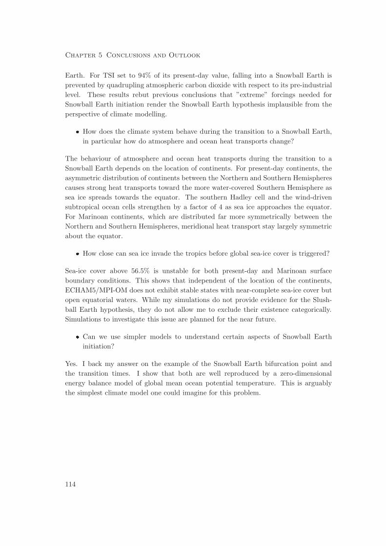
Chapter 5 Conclusions and Outlook
Earth. For TSI set to 94% of its present-day value, falling into a Snowball Earth is
prevented by quadrupling atmospheric carbon dioxide with respect to its pre-industrial
level. These results rebut previous conclusions that ”extreme” forcings needed for
Snowball Earth initiation render the Snowball Earth hypothesis implausible from the
perspective of climate modelling.� How does the climate system behave during the transition to a Snowball Earth,
in particular how do atmosphere and ocean heat transports change?
The behaviour of atmosphere and ocean heat transports during the transition to a
Snowball Earth depends on the location of continents. For present-day continents, the
asymmetric distribution of continents between the Northern and Southern Hemispheres
causes strong heat transports toward the more water-covered Southern Hemisphere as
sea ice spreads towards the equator. The southern Hadley cell and the wind-driven
subtropical ocean cells strengthen by a factor of 4 as sea ice approaches the equator.
For Marinoan continents, which are distributed far more symmetrically between the
Northern and Southern Hemispheres, meridional heat transport stay largely symmetric
about the equator.� How close can sea ice invade the tropics before global sea-ice cover is triggered?
Sea-ice cover above 56.5% is unstable for both present-day and Marinoan surface
boundary conditions. This shows that independent of the location of the continents,
ECHAM5/MPI-OM does not exhibit stable states with near-complete sea-ice cover but
open equatorial waters. While my simulations do not provide evidence for the Slush-
ball Earth hypothesis, they do not allow me to exclude their existence categorically.
Simulations to investigate this issue are planned for the near future.� Can we use simpler models to understand certain aspects of Snowball Earth
initiation?
Yes. I back my answer on the example of the Snowball Earth bifurcation point and
the transition times. I show that both are well reproduced by a zero-dimensional
energy balance model of global mean ocean potential temperature. This is arguably
the simplest climate model one could imagine for this problem.
114
5.2 Outlook
2. Atmospheric dynamics of a Snowball Earth� What characterizes the Hadley cell of a Snowball Earth atmosphere?
To ease comparison with theories, I focus on equinox insolation. I find that, in con-
trast to today’s atmosphere, vertical momentum diffusion is an important process in
the upper branch of a Snowball Earth Hadley cell. Consistent with thought exper-
iments, suppressing vertical diffusion of zonal momentum effects a weakening of the
Hadley cell whereas suppressing vertical diffusion of meridional momentum results in
a strengthening of the Hadley cell. Combining both effect shows that vertical diffusion
of meridional momentum exerts a stronger influence on the Snowball Earth Hadley cell
strength than vertical diffusion of zonal momentum.� How does this compare to dry Hadley cell theories?
I conclude that neither axisymmetric Hadley cell models based on angular momentum
conservation nor eddy-permitting Hadley cell models that neglect vertical diffusion
of momentum are applicable to a Snowball Earth atmosphere since both assume an
inviscid upper Hadley cell branch. Because vertical diffusion is important for the Hadley
cell of a Snowball Earth atmosphere, and because a Snowball Earth atmosphere is an
example for a dry atmosphere, dry atmospheres in general should not be considered as
a-priori simpler testcases for Hadley cell theories than moist atmospheres.
5.2 Outlook
In the end, I would like to propose two near-future modelling studies. The first targets
the Snowball versus Slushball debate. While my simulations provide support for the
Snowball Earth hypothesis, additional ECHAM5/MPI-OM simulations are needed to
judge the compatibility of the Slushball Earth hypothesis with climate physics. The
ultimate test of the Slushball Earth hypothesis would require to include interactive
ice-sheets in our simulations. This would allow us to verify if tropical glaciers at sea-
level form for some range of radiative forcing without triggering global sea-ice cover.
However, this clearly represents a major modelling effort. A simpler modelling strategy
that does not invoke interactive ice-sheets would be to prescribe all land as being
glaciated, and to use ECHAM5/MPI-OM to test if tropical land temperatures below
freezing are compatible with open equatorial oceans. If we find that this is not the
case, this will provide strong evidence against the Slushball Earth hypothesis, and even
more support for a Snowball Earth.
The second direction aims at the Hadley cell dynamics of dry atmospheres. I show
that vertical diffusion of momentum is important for the Snowball Earth Hadley cell
115
Chapter 5 Conclusions and Outlook
under equinox insolation. Motivated by the work of Walker and Schneider (2005, 2006),
who found that the influence of eddies on the Hadley cell depends on the latitude of the
insolation maximum, I propose to repeat our study for solstice insolation. Moreover,
the Snowball Earth atmosphere offers a straightforward testcase for dry atmospheres
because its boundary conditions largely eliminate moisture from the atmosphere and
therefore allowed me to apply a state-of-the art moist atmospheric general circulation
model to study a dry atmosphere. In future studies, it might however turn out beneficial
to transform the model into a dry model by manually switching off moist physics. This
would allow us to investigate dry atmospheres beyond the range of the Snowball Earth
framework.
116
Bibliography
Abbot, D. and I. Halevy, 2010: Dust Aerosol Important for Snowball Earth Deglacia-
tion. Journal of Climate, accepted.
Abbot, D. S. and R. T. Pierrehumbert, 2010: Mudball: Surface dust and Snowball
Earth deglaciation. Journal of Geophysical Research, 115.
Arakawa, A. and V. R. Lamb, 1977: Computational design of the basic dynamical
processes of the UCLA general circulation model. Methods Comput. Phys., 17, 173–
265.
Baum, S. K. and T. J. Crowley, 2001: GCM response to late precambrian (similar to
590 Ma) ice-covered continents. Geophysical Research Letters, 28 (4), 583–586.
Bengtsson, L., K. I. Hodges, and E. Roeckner, 2006: Storm tracks and climate change.
Journal of Climate, 19 (15), 3518–3543.
Berger, A. L., 1978: Long Term Variations of Daily Insolation and Quaternary Climatic
Changes. Journal of the Atmospheric Sciences, 35 (12), 2362–2367.
Brasseur, G. P. and E. Roeckner, 2005: Impact of improved air quality on the future
evolution of climate. Geophysical Research Letters, 32 (23), L23 704.
Bretagnon, P. and G. Francou, 1988: Planetary theories in rectangular and spherical
variables - Vsop-87 solutions. Astronomy and Astrophysics, 202 (1-2), 309–315.
Brinkop, S. and E. Roeckner, 1995: Sensitivity of a general-circulation model to pa-
rameterizations of cloud-turbulence interactions in the atmospheric boundary layer.
Tellus Series A-Dynamic Meteorology and Oceanography, 47 (2), 197–220.
Bronstein, I. N., 1996: Teubner-Taschenbuch der Mathematik. B. G. Teubner.
Budyko, M. I., 1969: Effect of solar radiation variations on climate of Earth. Tellus,
21 (5), 611–619.
Caballero, R., R. T. Pierrehumbert, and J. L. Mitchell, 2008: Axisymmetric, nearly
inviscid circulations in non-condensing radiative-convective atmospheres. Quarterly
Journal of the Royal Meteorological Society, 134 (634), 1269–1285.
117
Bibliography
Chandler, M. A. and L. E. Sohl, 2000: Climate forcings and the initiation of low-
latitude ice sheets during the Neoproterozoic Varanger glacial interval. Journal of
Geophysical Research-Atmospheres, 105 (D16), 20 737–20 756.
Crowley, T. J., W. T. Hyde, and W. R. Peltier, 2001: CO2 levels required for deglacia-
tion of a ”Near-Snowball” Earth. Geophysical Research Letters, 28 (2), 283–286.
Donnadieu, Y., Y. Godderis, G. Ramstein, A. Nedelec, and J. Meert, 2004a: A ’snow-
ball Earth’ climate triggered by continental break-up through changes in runoff.
Nature, 428 (6980), 303–306.
Donnadieu, Y., G. Ramstein, F. Fluteau, D. Roche, and A. Ganopolski, 2004b: The
impact of atmospheric and oceanic heat transports on the sea-ice-albedo instability
during the Neoproterozoic. Climate Dynamics, 22 (2-3), 293–306.
Enderton, D. and J. Marshall, 2009: Controls on the total dynamical heat transport of
the atmosphere and oceans. to appear in Journal of Atmospheric Sciences.
Evans, D. A. D., 2000: Stratigraphic, geochronological, and paleomagnetic constraints
upon the Neoproterozoic climatic paradox. American Journal of Science, 300 (5),
347–433.
Ferreira, D., B. Rose, and J. Marshall, 2009: In preparation.
Fischer, N. and J. H. Jungclaus, 2010: Effects of orbital forcing on atmosphere and
ocean heat transports in Holocene and Eemian climate simulations with a compre-
hensive Earth system model. Climate of the Past, 6 (2), 155–168.
Fortuin, J. P. F. and H. Kelder, 1998: An ozone climatology based on ozonesonde and
satellite measurements. Journal of Geophysical Research-Atmospheres, 103 (D24),
31 709–31 734.
Fouquart, Y. and B. Bonnel, 1980: Computations of solar heating of the earth’s atmo-
sphere: A new parametrization. Beitr. Phys. Atmos., 53, 35–62.
Fraedrich, K., 1979: Catastrophes and Resilience of a zero-dimensional climate system
with ice-albedo and greenhouse feedback. Quarterly Journal of the Royal Meteoro-
logical Society, 105 (443), 147–167.
Gamo, M., 1996: Thickness of the dry convection and large-scale subsidence above
deserts. Boundary-Layer Meteorology, 79 (3), 265–278.
Gent, P. R., J. Willebrand, T. J. McDougall, and J. C. McWilliams, 1995: Parameter-
izing eddy-induced tracer transports in ocean circulation models. Journal of Physical
Oceanography, 25 (4), 463–474.
118
Bibliography
Godderis, Y. and Y. Donnadieu, 2008: Carbon cycling and snowball Earth. Nature,
456 (7224).
Godderis, Y., et al., 2007: Coupled modeling of global carbon cycle and climate in
the Neoproterozoic: links between Rodinia breakup and major glaciations. Comptes
Rendus Geoscience, 339 (3-4), 212–222.
Goodman, J. C. and R. T. Pierrehumbert, 2003: Glacial flow of floating marine ice in
”Snowball Earth”. Journal of Geophysical Research-Oceans, 108 (C10), 3308.
Gough, D. O., 1981: Solar interior structure and luminosity variations. Solar Physics,
74 (1), 21–34, doi:10.1007/BF00151270.
Griffies, S. M., 1998: The Gent-McWilliams skew flux. Journal of Physical Oceanogra-
phy, 28 (5), 831–841.
Hagemann, S., 2002: MPI-Report 336: An improved land surface parameter dataset for
global and regional climate models. Tech. rep., Max Planck Institute for Meteorology,
Hamburg, Germany.
Hagemann, S., B. Machenhauer, R. Jones, O. B. Christensen, M. Deque, D. Jacob,
and P. L. Vidale, 2004: Evaluation of water and energy budgets in regional climate
models applied over Europe. Climate Dynamics, 23 (5), 547–567.
Heinemann, M., J. H. Jungclaus, and J. Marotzke, 2009: Warm Paleocene/Eocene
climate as simulated in ECHAM5/MPI-OM. Climate of the Past, 5 (3), 785–802.
Held, I. M., 2000: The general circulation of the atmosphere. Proc. Prog. Geophys.
Fluid. Dyn., Woods Hole, MA, USA, Woods Hole Oceanographic Institution, avail-
able under http://www.whoi.edu.
Held, I. M., 2001: The partitioning of the poleward energy transport between the
tropical ocean and atmosphere. Journal of the Atmospheric Sciences, 58 (8), 943–
948.
Held, I. M. and A. Y. Hou, 1980: Non-linear axially-symmetric circulations in a nearly
inviscid atmosphere. Journal of the Atmospheric Sciences, 37 (3), 515–533.
Held, I. M. and M. J. Suarez, 1974: Simple albedo feedback models of ice-caps. Tellus,
26 (6), 613–629.
Hernandez-Deckers, D. and J. S. von Storch, 2010: Energetics responses to in-
creases in greenhouse gas concentration. Journal of Climate, (2010), doi:
10.1175%2F2010JCLI3176.1, in press.
119
Bibliography
Hibler, W. D., 1979: Dynamic thermodynamic sea ice model. Journal of Physical
Oceanography, 9 (4), 815–846.
Hoffman, P. F., J. W. Crowley, D. T. Johnston, D. S. Jones, and D. P. Schrag, 2008:
Snowball prevention questioned. Nature, 456 (7224).
Hoffman, P. F., A. J. Kaufman, G. P. Halverson, and D. P. Schrag, 1998: A Neopro-
terozoic snowball earth. Science, 281 (5381), 1342–1346.
Hoffman, P. F. and D. P. Schrag, 2002: The snowball Earth hypothesis: testing the
limits of global change. Terra Nova, 14 (3), 129–155.
Holton, J. R., 2004: An Introduction to Dynamical Meteorology. Elsevier Academic
Press.
Hyde, W. T., T. J. Crowley, S. K. Baum, and W. R. Peltier, 2000: Neoprotero-
zoic ’snowball Earth’ simulations with a coupled climate/ice-sheet model. Nature,
405 (6785), 425–429.
Jenkins, G. S. and L. A. Frakes, 1998: GCM sensitivity test using increased rotation
rate, reduced solar forcing and orography to examine low latitude glaciation in the
Neoproterozoic. Geophysical Research Letters, 25 (18), 3525–3528.
Jungclaus, J. H., et al., 2006: Ocean circulation and tropical variability in the coupled
model ECHAM5/MPI-OM. Journal of Climate, 19 (16), 3952–3972.
Kaufman, A. J., 2007: Palaeoclimate: Slush find. Nature, 450 (7171), 807–808, doi:
10.1038/450807a.
Kerr, R. A., 2010: Snowball Earth has melted back to a profound wintry mix. Science,
327 (5970), 1186–, doi:10.1126/science.327.5970.1186.
Kim, H. K. and S. Lee, 2001: Hadley cell dynamics in a primitive equation model. Part
I: Axisymmetric flow. Journal of the Atmospheric Sciences, 58 (19), 2845–2858.
Kirschvink, J. L., 1992: The Proterozoic Biosphere, chap. Late Proterozoic low-latitude
global glaciation: The snowball Earth, 51–52. Cambridge University Press, New
York.
Korty, R. L. and T. Schneider, 2008: Extent of Hadley circulations in dry atmospheres.
Geophysical Research Letters, 35 (23), L23 803.
Landerer, F. W., J. H. Jungclaus, and J. Marotzke, 2007: Regional dynamic and
steric sea level change in response to the IPCC-A1B scenario. Journal of Physical
Oceanography, 37 (2), 296–312.
120
Bibliography
Le Hir, G., Y. Donnadieu, Y. Godderis, R. T. Pierrehumbert, G. R. Halverson, M. Ma-
couin, A. Nedelec, and G. Ramstein, 2009: The snowball Earth aftermath: Exploring
the limits of continental weathering processes. Earth and Planetary Science Letters,
277 (3-4), 453–463.
Le Hir, G., Y. Donnadieu, G. Krinner, and G. Ramstein, 2010: Toward the snowball
earth deglaciation. Climate Dynamics, doi:10.1007/s00382-010-0748-8.
Le Hir, G., G. Ramstein, Y. Donnadieu, and R. T. Pierrehumbert, 2007: Investigating
plausible mechanisms to trigger a deglaciation from a hard snowball Earth. Comptes
Rendus Geoscience, 339 (3-4), 274–287.
Lewis, J. P., A. J. Weaver, and M. Eby, 2007: Snowball versus slushball Earth: Dynamic
versus nondynamic sea ice? Journal of Geophysical Research-Oceans, 112 (C11),
C11 014, doi:10.1029/2006JC004037.
Lewis, J. P., A. J. Weaver, S. T. Johnston, and M. Eby, 2003: Neoproterozoic ”snowball
Earth”: Dynamic sea ice over a quiescent ocean. Paleoceanography, 18 (4), 1092.
Lin, S. J. and R. B. Rood, 1996: Multidimensional flux-form semi-Lagrangian transport
schemes. Monthly Weather Review, 124 (9), 2046–2070.
Lohmann, U. and E. Roeckner, 1996: Design and performance of a new cloud mi-
crophysics scheme developed for the ECHAM general circulation model. Climate
Dynamics, 12 (8), 557–572.
Lorenz, E. N., 1967: The Nature and Theory of the General Circulation of the Atmo-
sphere. World Meteorological Organization.
Lott, F. and M. J. Miller, 1997: A new subgrid-scale orographic drag parametrization:
Its formulation and testing. Quarterly Journal of the Royal Meteorological Society,
123 (537), 101–127.
Louis, J. F., 1979: Parametric model of vertical eddy fluxes in the atmosphere.
Boundary-Layer Meteorology, 17 (2), 187–202.
Lubick, N., 2002: Palaeoclimatology: Snowball fights. Nature, 417 (6884), 12–13,
doi:10.1038/417012a.
Luo, J. J., S. Masson, E. Roeckner, G. Madec, and T. Yamagata, 2005: Reducing
climatology bias in an ocean-atmosphere CGCM with improved coupling physics.
Journal of Climate, 18 (13), 2344–2360.
Macdonald, F. A., et al., 2010: Calibrating the Cryogenian. Science, 327 (5970),
1241–1243, doi:10.1126/science.1183325.
121
Bibliography
Marotzke, J. and M. Botzet, 2007: Present-day and ice-covered equilibrium states
in a comprehensive climate model. Geophysical Research Letters, 34 (16), doi:
10.1029/2006GL028880.
Marshall, J., D. Ferreira, J. M. Campin, and D. Enderton, 2007: Mean climate and
variability of the atmosphere and ocean on an aquaplanet. Journal of the Atmospheric
Sciences, 64 (12), 4270–4286.
Marsland, S. J., H. Haak, J. H. Jungclaus, M. Latif, and F. Roske, 2003: The Max-
Planck-Institute global ocean/sea ice model with orthogonal curvilinear coordinates.
Ocean Modelling, 5 (2), 91–127.
Medeiros, B., A. Hall, and B. Stevens, 2005: What controls the mean depth of the
PBL? Journal of Climate, 18 (16), 3157–3172.
Micheels, A. and M. Montenari, 2008: A snowball Earth versus a slushball Earth:
Results from Neoproterozoic climate modeling sensitivity experiments. Geosphere,
4 (2), 401–410.
Mlawer, E. J., S. J. Taubman, P. D. Brown, M. J. Iacono, and S. A. Clough, 1997:
Radiative transfer for inhomogeneous atmospheres: RRTM, a validated correlated-k
model for the longwave. Journal of Geophysical Research-Atmospheres, 102 (D14),
16 663–16 682.
Myhre, G., E. J. Highwood, K. P. Shine, and F. Stordal, 1998: New estimates of
radiative forcing due to well mixed greenhouse gases. Geophysical Research Letters,
25 (14), 2715–2718, doi:10.1029/98GL01908.
Neale, R. B. and B. J. Hoskins, 2000a: A standard test for AGCMs and their physical
parameterizations. I: The proposal. Atmos. Sci. Letters, 1, 101–107.
Neale, R. B. and B. J. Hoskins, 2000b: A standard test for AGCMs and their physical
parameterizations. II: Results for The Met. Office Model. Atmos. Sci. Letters, 1,
108–114.
Nordeng, T. E., 1994: Extended versions of the convective parametrization scheme at
ECMWF and their impact on the mean and transient activity of the model in the
tropics. Technical memorandum 206, ECMWF, Reading, UK.
North, G. R., 1975: Analytical Solution to a simple climate model with diffusive heat
transport. Journal of the Atmospheric Sciences, 32 (7), 1301–1307.
Pacanowski, R. C. and S. G. H. Philander, 1981: Parameterization of vertical mixing
in numerical models of tropical oceans. Journal of Physical Oceanography, 11 (11),
1443–1451.
122
Bibliography
Peixoto, J. P. and A. H. Oort, 1992: Physics of Climate. American Institute of Physics.
Peltier, W. R., 2003: Earth System History. Encyclopedia of Global Environmental
Change, Volume 1, The Earth System: Physical and Chemical Dimensions of Global
Environmental Change, M. C. MacCracken and J. S. Perry, Eds., John Wiley & Sons,
31–60.
Peltier, W. R. and Y. G. Liu, 2008: Carbon cycling and snowball Earth Reply. Nature,
456 (7224).
Peltier, W. R., Y. G. Liu, and J. W. Crowley, 2007: Snowball Earth prevention by
dissolved organic carbon remineralization. Nature, 450 (7171), 813–U1.
Peltier, W. R., L. Tarasov, G. Vettoretti, and L. P. Solheim, 2004: Climate dynamics in
deep time: Modeling the ”Snowball bifurcation” and assessing the plausibility of its
occurrence. Extreme Proterozoic Geology, Geochemistry and Climate, 146, 107–124.
Pierrehumbert, R. T., 2002: The hydrologic cycle in deep-time climate problems. Na-
ture, 419 (6903), 191–198.
Pierrehumbert, R. T., 2005: Climate dynamics of a hard snowball Earth. Journal of
Geophysical Research-Atmospheres, 110 (D1), D01 111.
Pierrehumbert, R. T., 2010: Planetary climates. Cambridge University Press.
Pollard, D. and J. F. Kasting, 2005: Snowball Earth: A thin-ice solution with flowing
sea glaciers. Journal of Geophysical Research-Oceans, 110 (C7), C07 010.
Poulsen, C. J., 2003: Absence of a runaway ice-albedo feedback in the Neoproterozoic.
Geology, 31 (6), 473–476.
Poulsen, C. J. and R. L. Jacob, 2004: Factors that inhibit snowball Earth simulation.
Paleoceanography, 19 (4), PA4021.
Poulsen, C. J., R. L. Jacob, R. T. Pierrehumbert, and T. T. Huynh, 2002: Testing
paleogeographic controls on a Neoproterozoic snowball Earth. Geophysical Research
Letters, 29 (11), 1515, doi:10.1029/2001GL014352.
Poulsen, C. J., R. T. Pierrehumbert, and R. L. Jacob, 2001: Impact of ocean dynamics
on the simulation of the Neoproterozoic ”snowball Earth”. Geophysical Research
Letters, 28 (8), 1575–1578.
Randall, D. A., J. A. Abeles, and T. G. Corsetti, 1985: Seasonal simulations of the
planetary boundary layer and boundary layer stratocumulus clouds with a general
circulation model. Journal of the Atmospheric Sciences, 42 (7), 641–676.
123
Bibliography
Raval, A. and V. Ramanathan, 1989: Observational determination of the greenhouse
effect. Nature, 342 (6251), 758–761.
Roeckner, 2007: EH5-T31L19 MPIOM-GR3.0L40 PIcntrl. World Data
Center for Climate. CERA-DB ”EH5-T31L19 OM-GR3.0L40 CTL”.
http://cera-www.dkrz.de/WDCC/ui/Compact.jsp?acronym=EH5-T31L19 OM-
GR3.0L40 CTL.
Roeckner, E., et al., 2003: The atmospheric general circulation model ECHAM5, part
I: Model description. Tech. rep., Max Planck Institute for Meteorology, Hamburg,
Germany.
Roeckner, E., et al., 2006: Sensitivity of simulated climate to horizontal and vertical
resolution in the ECHAM5 atmosphere model. Journal of Climate, 19 (16), 3771–
3791.
Romanova, V., G. Lohmann, and K. Grosfeld, 2006: Effect of land albedo, CO2, orog-
raphy, and oceanic heat transport on extreme climates. Climate of the Past, 2 (1),
31–42.
Rose, B. E. J. and J. Marshall, 2009: Ocean heat transport, sea ice, and multiple climate
states: insights from energy balance models. accepted for publication in Journal of
the Atmospheric Sciences.
Rothman, D. H., J. M. Hayes, and R. E. Summons, 2003: Dynamics of the Neopro-
terozoic carbon cycle. Proceedings of the National Academy of Sciences of the United
States of America, 100 (14), 8124–8129.
Savijarvi, H., 2009: Stable boundary layer: Parametrizations for local and larger scales.
Quarterly Journal of the Royal Meteorological Society, 135 (641), 914–921.
Schneider, E. K., 1977: Axially-symmetric steady-state models of basic state for insta-
bility and climate studies. Part II. Nonlinear calculations. Journal of the Atmospheric
Sciences, 34 (2), 280–296.
Schneider, T., 2004: The tropopause and the thermal stratification in the extratropics
of a dry atmosphere. Journal of the Atmospheric Sciences, 61 (12), 1317–1340.
Schneider, T., 2006: The general circulation of the atmosphere. Annual Review of Earth
and Planetary Sciences, 34, 655–688.
Schneider, T. and C. C. Walker, 2006: Self-organization of atmospheric macroturbu-
lence into critical states of weak nonlinear eddy-eddy interactions. Journal of the
Atmospheric Sciences, 63 (6), 1569–1586.
124
Bibliography
Sellers, W. D., 1969: A global climate model based on the energy balance of the Earth-
atmosphere system. Journal of Applied Meteorology, 8, 392–400.
Semtner, A. J., 1976: Model for thermodynamic growth of sea ice in numerical inves-
tigations of climate. Journal of Physical Oceanography, 6 (3), 379–389.
Smith, R. S., C. Dubois, and J. Marotzke, 2006: Global climate and ocean circulation
on an aquaplanet ocean-atmosphere general circulation model. Journal of Climate,
19 (18), 4719–4737.
Solomon, S., D. Qin, M. Manning, Z. Chen, M. Marquis, K. B. Averyt, T. M., and H. L.
Miller, (Eds.) , 2007: Contribution of Working Group I to the Fourth Assessment
Report of the Intergovernmental Panel on Climate Change, 2007. Cambridge Univ.
Press, Cambridge, U. K.
Stone, P. H., 1978: Constraints on dynamical transports of energy on a spherical planet.
Dynamics of Atmospheres and Oceans, 2 (2), 123–139.
Stone, P. H. and M. S. Yao, 2004: The ice-covered Earth instability in a model of
intermediate complexity. Climate Dynamics, 22 (8), 815–822.
Tanre, D., J. F. Geleyn, and J. Slingo, 1984: First results of the introduction of an
advanced aerosol-radiation interaction in ECMWF low resolution global model, 133–
177. Deepak Publishing, Hampton, VA.
Tiedtke, M., 1989: A comprehensive mass flux scheme for cumulus parameterization in
large-scale models. Monthly Weather Review, 117 (8), 1779–1800.
Trindade, R. I. F. and M. Macouin, 2007: Palaeolatitude of glacial deposits and palaeo-
geography of Neoproterozoic ice ages. Comptes Rendus Geoscience, 339 (3-4), 200–
211.
Valcke, S., A. Caubel, D. Declat, and L. Terray, 2003: OASIS Ocean Atmosphere Sea
Ice Soil users’s guide. Tech. rep., CERFACS Tech. Rep. TR/CMGC/03/69, Toulouse,
France, 85 pp.
Vallis, G. K., 2006: Atmosphericv and Oceanic Fluid Dynamics. Cambridge University
Press.
Voigt, A. and J. Marotzke, 2009: The transition from the present-day climate to a
modern Snowball Earth. Climate Dynamics, doi:10.1007/s00382-009-0633-5.
Walker, C. C. and T. Schneider, 2005: Response of idealized Hadley circulations to
seasonally varying heating. Geophysical Research Letters, 32 (6), L06 813.
125
Bibliography
Walker, C. C. and T. Schneider, 2006: Eddy influences on Hadley circulations: Sim-
ulations with an idealized GCM. Journal of The Atmospheric Sciences, 63 (12),
3333–3350.
Walsh, K. J. and W. D. Sellers, 1993: Response of a global climate model to a 30 percent
reduction of the solar constant. Global and Planetary Change, 8 (4), 219–230.
Washington, W. M. and C. L. Parkinson, 2005: An Introduction to Three-Dimensional
Climate Modeling. 2d ed., University Science Books.
Wild, M. and E. Roeckner, 2006: Radiative fluxes in the ECHAM5 general circulation
model. Journal of Climate, 19 (16), 3792–3809.
Wolff, J. O., E. Maier-Reimer, and S. Legutke, 1997: The Hamburg Ocean Primitive
Equation Model HOPE. Tech. Rep. 13. Tech. rep., German Climate Computer Center
(DKRZ), Hamburg, Germany.
Zilitinkevich, S. S., V. L. Perov, and J. C. King, 2002: Near-surface turbulent fluxes
in stable stratification: Calculation techniques for use in general-circulation models.
Quarterly Journal of the Royal Meteorological Society, 128 (583), 1571–1587.
126
Acknowledgements
First and foremost, I wish to thank Prof. Dr. Jochem Marotzke for being an excellent
supervisor. He granted scientific freedom as much as possible but pulled me back on
track whenever I needed it. I especially thank him for teaching me how to think simple
to understand the complex, and for opening doors that would otherwise have remained
closed. I would like to thank my co-advisor Dr. Erich Roeckner for numerous discus-
sions and help with ECHAM5. Thanks to Prof. Dr. Hans von Storch for chairing my
panel and for driving me to focus my floating thoughts.
I would like to thank the IMPRS-ESM for providing an outstanding PhD environment.
Special thanks to Dr. Antje Weitz and Cornelia Kampmann for their organisational
and mental support. I also thank the ZEIT Foundation Ebelin and Gerd Bucerius
for funding the IMPRS-ESM Guest and Exchange Program, which made the visit of
Dr. Dorian Abbot to Hamburg possible, as well as several trips of my own. Thanks to
the German Climate Computing Centre (DKRZ), and to the Central IT Services for
their technical support. I thank the library staff for getting hold of whatever books I
needed, and for keeping track of the drum room key.
I would like to express my gratitude to Prof. Dr. Issac M. Held for first-hand insight
into the world of Hadley cells and his kind hospitality during my stay at GFDL. This
paved my way into atmospheric dynamics. I wish to thank Dr. Dorian S. Abbot and
Prof. Dr. Raymond T. Pierrehumbert for providing the Marinoan reconstruction and
innumerous advice on the Marinoan Snowball Earth simulations. I would also like
to thank Dr. Thorsten Mauritsen for suggesting the short-tail stability function, and
Prof. Dr. Bjorn Stevens for help with setting up the 62-level ECHAM5 grid. Many
thanks go to Michael Botzet and Dr. Helmuth Haak for help with running and analyz-
ing the coupled model and their interest in my work. I thank the ocean group and the
MPI-M in general for creating a supporting and productive atmosphere.
Thanks especially to Ilka Wantia, Dr. Malte Heinemann, Nils Fischer, Florian Rauser,
Fanny Adloff, Steffen Tietsche, Mario Krapp, Ronny Petrik, Maria Paz Chidichimo,
127

Acknowledgements
Daniel Hernandez-Deckers, Freja Vamborg, Juliane Otto, Werner Bauer, Rosina Grimm,
Jaison Ambadan, and Peter Duben for cheering me up, making me feel comfortable in
Hamburg, and for braving tired jokes.
There is little more to say, but this little is so all-embracing, Gabriela, that I lacked
the words until I remembered these.
I never planned in my imagination a situation so heavenly
A fairy land where no one else could enter
And in the center just you and me
My heart beat like a hammer
My arms wound around you tight
And stars fell on Taiga last night.
128


Die gesamten Veröffentlichungen in der Publikationsreihe des MPI-M„Berichte zur Erdsystemforschung“,„Reports on Earth System Science“, ISSN 1614-1199
sind über die Internetseiten des Max-Planck-Instituts für Meteorologie erhältlich:
http://www.mpimet.mpg.de/wissenschaft/publikationen.html

ISSN 1614-1199


