
Smoothing and Equating Methods Applied to Different … and Equating Methods Applied to Different...
32
Smoothing and Equating Methods Applied to Different Types of Test Score Distributions and Evaluated With Respect to Multiple Equating Criteria Tim Moses Jinghua Liu April 2011 Research Report ETS RR–11-20
-
Upload
truongtram -
Category
Documents
-
view
219 -
download
1
Transcript of Smoothing and Equating Methods Applied to Different … and Equating Methods Applied to Different...
Smoothing and Equating Methods Applied to Different Types of Test Score Distributions and Evaluated With Respect to Multiple Equating Criteria
Tim Moses
Jinghua Liu
April 2011
Research Report ETS RR–11-20

Smoothing and Equating Methods Applied to Different Types of Test Score
Distributions and Evaluated With Respect to Multiple Equating Criteria
Tim Moses and Jinghua Liu
ETS, Princeton, New Jersey
April 2011

Technical Review Editor: Daniel Eignor
Technical Reviewers: Samuel A. Livingston and Rick Morgan
Copyright © 2011 by Educational Testing Service. All rights reserved.
ETS, the ETS logo, and LISTENING. LEARNING. LEADING. are registered trademarks of Educational Testing
Service (ETS).
As part of its nonprofit mission, ETS conducts and disseminates the results of research to advance
quality and equity in education and assessment for the benefit of ETS’s constituents and the field.
To obtain a PDF or a print copy of a report, please visit:
http://www.ets.org/research/contact.html

i
Abstract
In equating research and practice, equating functions that are smooth are typically
assumed to be more accurate than equating functions with irregularities. This assumption
presumes that population test score distributions are relatively smooth. In this study, two
examples were used to reconsider common beliefs about smoothing and equating. The
first example involves a relatively smooth population test score distribution and the
second example involves a population test score distribution with systematic
irregularities. Various smoothing and equating methods (presmoothing, equipercentile,
kernel, and postsmoothing) were compared across the two examples with respect to how
well the test score distributions were reflected in the equating functions, the smoothness
of the equating functions, and the standard errors of equating. The smoothing and
equating methods performed more similarly in the first example than in the second
example. The results of the second example illustrate that when dealing with
systematically irregular test score distributions, smoothing and equating methods can be
used in different ways to satisfy different equating criteria.
Key words: equipercentile equating, presmoothing, postsmoothing, equating criteria

ii
Table of Contents
Smoothing Methods ........................................................................................................ 1
Types of Test Score Distributions ................................................................................... 2
Equating Criteria ............................................................................................................. 2
This Study ....................................................................................................................... 3
First Example: Equating With Smooth Test Data ........................................................... 4
Considered Smoothing and Equating Methods............................................................... 5
Comparing Equated Scores Produced by Different Methods ......................................... 6
Distribution-Matching and Lack of Smoothness ............................................................ 7
Standard Errors ............................................................................................................... 8
Summary of the Results of the First Equating Example ................................................. 9
Second Example: Equating With Systematically Irregular Test Data ............................ 9
Considered Smoothing and Equating Methods............................................................. 11
Comparing Methods’ Equated Scores .......................................................................... 13
Distribution-Matching and Lack of Smoothness .......................................................... 14
Standard Errors ............................................................................................................. 16
Summary of the Results of the Second Equating Example .......................................... 17
Discussion ......................................................................................................................... 17
References ......................................................................................................................... 20
Note ................................................................................................................................... 22
Appendix ............................................................................................................................23
iii
List of Figures
Figure 1. Y distribution: First equating example ..............................................................................4
Figure 2. Equating function differences from the linear function. ..................................................7
Figure 3. Equating function standard errors: First equating example. .............................................9
Figure 4. Transformed Y distribution: Second equating example. .................................................11
Figure 5. Equating function differences from the linear function: Second equating
example. ..........................................................................................................................14
Figure 6. Equating function standard errors. Second equating example. ......................................16
iv
List of Tables
Table 1 First Equating Example. .......................................................................................... 5
Table 2 First Equating Example: Rounded Equated Scores. ................................................ 6
Table 3 First Equating Example: Equating Results on Matching Y’s Distribution and
Lack of Smoothness. ................................................................................................ 8
Table 4 Second Equating Example: Transformed Y Data. ................................................. 10
Table 5 Second Equating Example: Rounded Equated Scores. .......................................... 13
Table 6 Second Equating Example: Equating Results on Matching the Transformed Y’s
Distribution and Lack of Smoothness. ................................................................... 15
1
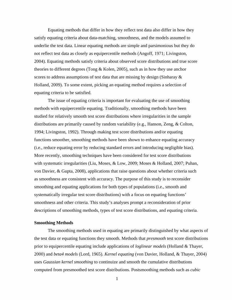
Equating methods that differ in how they reflect test data also differ in how they
satisfy equating criteria about data-matching, smoothness, and the models assumed to
underlie the test data. Linear equating methods are simple and parsimonious but they do
not reflect test data as closely as equipercentile methods (Angoff, 1971; Livingston,
2004). Equating methods satisfy criteria about observed score distributions and true score
theories to different degrees (Tong & Kolen, 2005), such as in how they use anchor
scores to address assumptions of test data that are missing by design (Sinharay &
Holland, 2009). To some extent, picking an equating method requires a selection of
equating criteria to be satisfied.
The issue of equating criteria is important for evaluating the use of smoothing
methods with equipercentile equating. Traditionally, smoothing methods have been
studied for relatively smooth test score distributions where irregularities in the sample
distributions are primarily caused by random variability (e.g., Hanson, Zeng, & Colton,
1994; Livingston, 1992). Through making test score distributions and/or equating
functions smoother, smoothing methods have been shown to enhance equating accuracy
(i.e., reduce equating error by reducing standard errors and introducing negligible bias).
More recently, smoothing techniques have been considered for test score distributions
with systematic irregularities (Liu, Moses, & Low, 2009; Moses & Holland, 2007; Puhan,
von Davier, & Gupta, 2008), applications that raise questions about whether criteria such
as smoothness are consistent with accuracy. The purpose of this study is to reconsider
smoothing and equating applications for both types of populations (i.e., smooth and
systematically irregular test score distributions) with a focus on equating functions’
smoothness and other criteria. This study’s analyses prompt a reconsideration of prior
descriptions of smoothing methods, types of test score distributions, and equating criteria.
Smoothing Methods
The smoothing methods used in equating are primarily distinguished by what aspects of
the test data or equating functions they smooth. Methods that presmooth test score distributions
prior to equipercentile equating include applications of loglinear models (Holland & Thayer,
2000) and beta4 models (Lord, 1965). Kernel equating (von Davier, Holland, & Thayer, 2004)
uses Gaussian kernel smoothing to continuize and smooth the cumulative distributions
computed from presmoothed test score distributions. Postsmoothing methods such as cubic

2
splines can be applied to produce a smoothed equating function from a raw equipercentile
function (Kolen & Brennan, 2004). Linear equating functions have also been described as
strong smoothing methods (Yang, Dorans, & Tateneni, 2003, p. 65) that are based on the means
and standard deviations of unsmoothed test score distributions. This study considers
presmoothing, kernel, and postsmoothing methods.
Types of Test Score Distributions
Different types of test score distributions can be assumed to come from populations that
are smooth or systematically irregular. Test score distributions from a test that is scored by
summing examinees’ correct responses to each item are usually assumed to reflect relatively
smooth populations, so that any irregularity in the sample data is attributed to sampling
variability. Some types of test score distributions have irregularities that are systematic due to
issues such as nonlinear scale transformations (Kolen & Brennan, 2004), formula scoring
based on subtracting a portion of examinees’ total incorrect responses from their total correct
responses (von Davier et al., 2004), and other scaling, weighting, rounding, and truncation
practices. For these distributions, irregularities could be attributed to sampling variability,
and/or to systematic structures that occur due to how the scores are produced.
Equating Criteria
Equipercentile equating and the use of smoothing in equating can be understood to
reflect competing goals and criteria. An equipercentile equating function that maps the
scores of test X to test Y’s scale is intended to produce an equated score distribution that
matches Y’s distribution for some target group of test takers (Angoff, 1971; von Davier et
al., 2004; Kolen & Brennan, 2004). To some extent, the application of smoothing
undermines the distribution-matching goal of equipercentile equating, in that the smooth
equating function can reflect smoothness criteria more directly than the matching of Y’s
distribution. Nonetheless, the pursuit of smoothness in equating is typically associated
with enhanced equating accuracy, as equating texts have suggested that irregularities in an
equating function are indicative of “considerable error” (Kolen & Brennan, 2004, p. 67).
The tradeoff of distribution-matching and smoothness for a given equating situation
has a statistical analogue that pertains to the bias and variability of a sample equating
function. The tradeoff of bias and variability in smoothing and equating applications
3
corresponds to choices in smoothing and equating to match more or less of Y’s distribution
and to produce a sample equating function which is more or less biased and less or more
variable (Holland, 2007; Kolen & Brennan, 2004). In simulation studies, the application of
smoothing is typically shown to reduce total equating error, or the sum of equating function
variability and squared bias (Hanson et al., 1994; Livingston, 1992). The implications of
simulation research are that smoothing applications only minimally interfere with the
distribution-matching goals of equipercentile equating, thereby reducing total equating error
by reducing equating variability and introducing minimal equating bias.
This Study
This study reconsiders the notion that making equating functions smoother will
also make them more accurate. Smoothing and equating methods such as presmoothing,
equipercentile, kernel, and postsmoothing methods are applied in two equating examples,
one involving a population test score distribution that is smooth and the other involving a
population test score distribution with systematic irregularities. The methods’ equating
functions are compared with respect to multiple criteria, including their degrees of
smoothness, their distribution-matching success, and their standard errors. This study’s
evaluations of multiple smoothing and equating methods for different types of test data
and with respect to multiple equating criteria provide useful replications and extensions of
prior studies’ results.
This study’s first example involving a smooth population distribution is expected to
produce results that are similar to those of prior smoothing and equating studies that have
considered smooth population distributions and have suggested that different smoothing
methods have similar accuracy benefits (Cui & Kolen, 2009; Hanson et al., 1994;
Livingston, 1992). The prior studies’ results are also extended in two ways. First, kernel
equating is included as one of the smoothing and equating methods being compared.
Second, comparisons of the smoothing and equating methods with respect to their
smoothness and distribution-matching properties are connected to comparisons of their
accuracies (standard errors).
This study’s second example involving a population distribution with systematic
irregularities extends the results of other smoothing studies that have considered
systematically irregular population distributions and the choices involved when using
4
different smoothing and equating methods (Liu et al., 2009; Moses & Holland, 2007;
Puhan et al., 2008). Whereas prior studies have focused on different loglinear
presmoothing models and the differences between traditional equipercentile and kernel
equating results, this study expands the focus to include postsmoothing methods. In
addition, the prior studies’ evaluative comparisons that have included distribution-
matching and smoothness comparisons (Liu et al., 2009), standard error comparisons
(Moses & Holland, 2007), and direct comparisons of equating functions (Puhan et al.,
2008) are all considered in a single set of results.
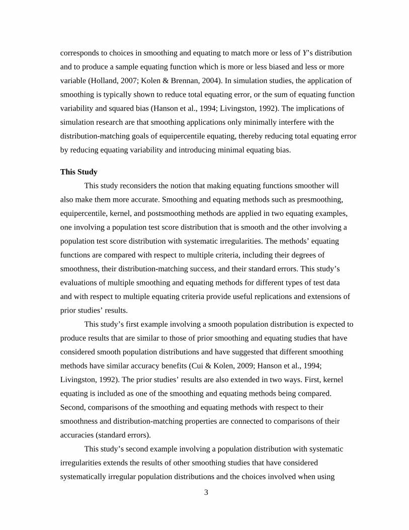
First Example: Equating With Smooth Test Data
For the situation of equating test data assumed to come from smooth populations,
the smoothing and equating methods of interest are applied to equate the two tests featured
in von Davier et al.’s (2004) single group data. These two tests, X and Y, were 20-item
rights-scored tests taken by one group of 1,453 examinees.
Figure 1. Y distribution: First equating example.
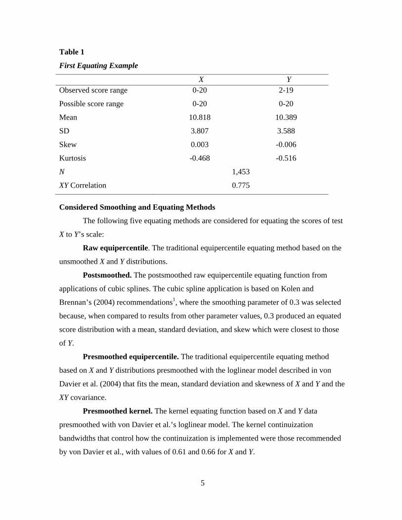
The descriptive characteristics of the data are summarized in Table 1. The unsmoothed
frequency distribution of test Y is plotted in Figure 1, showing irregularities that von
Davier et al. attribute to sampling instability that can be reduced using loglinear
presmoothing (p. 119).
0
0.02
0.04
0.06
0.08
0.1
0.12
0 5 10 15 20 25
Pro
ba
bil
ity
Y
5
Table 1
First Equating Example
X Y Observed score range 0-20 2-19
Possible score range 0-20 0-20
Mean 10.818 10.389
SD 3.807 3.588
Skew 0.003 -0.006
Kurtosis -0.468 -0.516
N 1,453
XY Correlation 0.775
Considered Smoothing and Equating Methods
The following five equating methods are considered for equating the scores of test
X to Y’s scale:
Raw equipercentile. The traditional equipercentile equating method based on the
unsmoothed X and Y distributions.
Postsmoothed. The postsmoothed raw equipercentile equating function from
applications of cubic splines. The cubic spline application is based on Kolen and
Brennan’s (2004) recommendations1, where the smoothing parameter of 0.3 was selected
because, when compared to results from other parameter values, 0.3 produced an equated
score distribution with a mean, standard deviation, and skew which were closest to those
of Y.
Presmoothed equipercentile. The traditional equipercentile equating method
based on X and Y distributions presmoothed with the loglinear model described in von
Davier et al. (2004) that fits the mean, standard deviation and skewness of X and Y and the
XY covariance.
Presmoothed kernel. The kernel equating function based on X and Y data
presmoothed with von Davier et al.’s loglinear model. The kernel continuization
bandwidths that control how the continuization is implemented were those recommended
by von Davier et al., with values of 0.61 and 0.66 for X and Y.

6
Linear. The linear equating based on the means and standard deviations of X and Y
(Table 1).
Comparing Equated Scores Produced by Different Methods
One way to evaluate the smoothing and equating methods of interest is to directly
compare their rounded scores. Table 2 shows that the equated and rounded scores based
on all of the considered smoothing and equating methods are almost completely identical.
Table 2
First Equating Example: Rounded Equated Scores
X
X-to-Y, raw
equipercentile X-to-Y,
postsmoothed
X-to-Y, presmoothed equipercentile
X-to-Y, presmoothed
kernel X-to-Y, linear
0 0 0 0 0 0 1 0 1 1 1 1 2 2 2 2 2 2 3 3 3 3 3 3 4 4 4 4 4 4 5 5 5 5 5 5 6 6 6 6 6 6 7 7 7 7 7 7 8 8 8 8 8 8 9 9 9 9 9 9 10 10 10 10 10 10 11 11 11 11 11 11 12 12 12 12 12 12 13 12 12 12 12 12 14 13 13 13 13 13 15 14 14 14 14 14 16 15 15 15 15 15 17 16 16 16 16 16 18 17 17 17 17 17 19 18 18 18 18 18 20 19 20 19 19 19
One exception is the relatively low equated score based on the raw equipercentile method at
the X score of 1. The other exception is the relatively high equated score based on the
postsmoothing method at the X score of 20, a result of Kolen and Brennan’s (2004, p. 86-87)
suggested linear function that binds the maximum X and Y scores at the ends of the score range
where data are sparse.
7
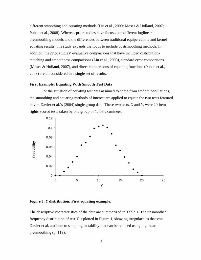
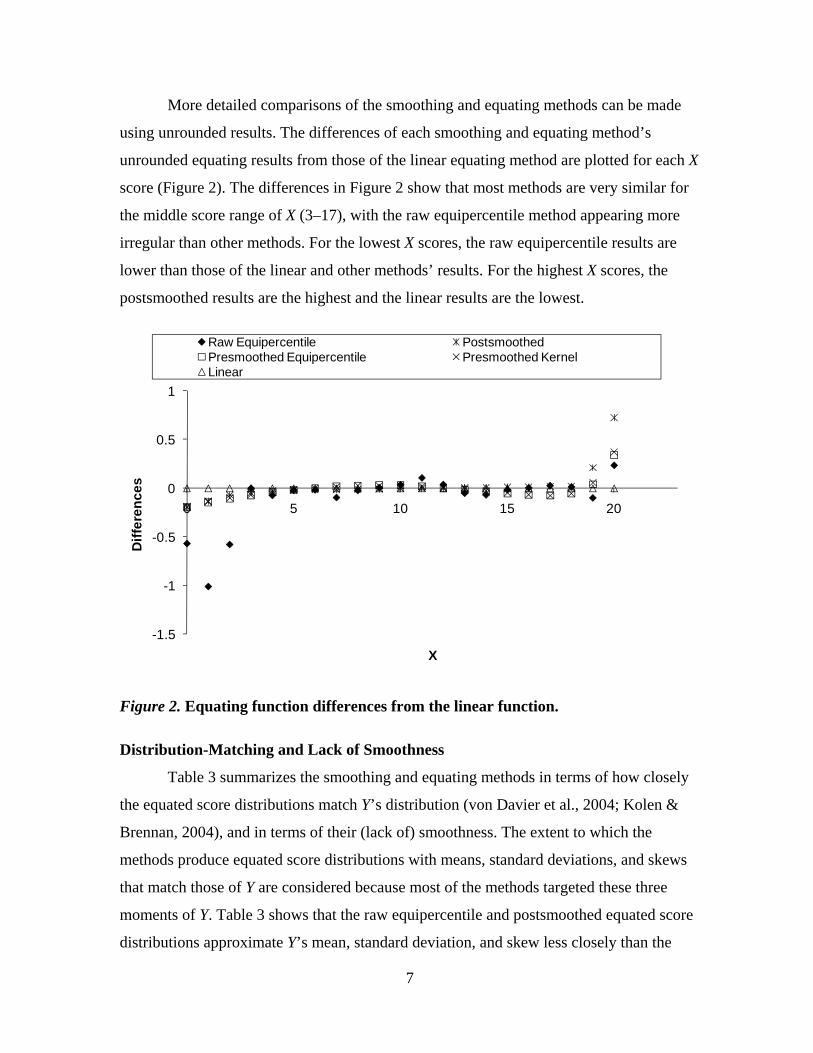
More detailed comparisons of the smoothing and equating methods can be made
using unrounded results. The differences of each smoothing and equating method’s
unrounded equating results from those of the linear equating method are plotted for each X
score (Figure 2). The differences in Figure 2 show that most methods are very similar for
the middle score range of X (3–17), with the raw equipercentile method appearing more
irregular than other methods. For the lowest X scores, the raw equipercentile results are
lower than those of the linear and other methods’ results. For the highest X scores, the
postsmoothed results are the highest and the linear results are the lowest.
Figure 2. Equating function differences from the linear function.
Distribution-Matching and Lack of Smoothness
Table 3 summarizes the smoothing and equating methods in terms of how closely
the equated score distributions match Y’s distribution (von Davier et al., 2004; Kolen &
Brennan, 2004), and in terms of their (lack of) smoothness. The extent to which the
methods produce equated score distributions with means, standard deviations, and skews
that match those of Y are considered because most of the methods targeted these three
moments of Y. Table 3 shows that the raw equipercentile and postsmoothed equated score
distributions approximate Y’s mean, standard deviation, and skew less closely than the
-1.5
-1
-0.5
0
0.5
1
0 5 10 15 20
Dif
fere
nc
es
X
Raw Equipercentile PostsmoothedPresmoothed Equipercentile Presmoothed KernelLinear

8
other methods. The linear and presmoothed kernel methods’ means and standard
deviations deviate relatively little from the mean and standard deviation of Y, whereas the
presmoothed kernel and presmoothed equipercentile methods’ skews deviate relatively
little from the skew of Y. Table 3 reports methods’ lack of smoothness using Liu et al.’s
(2009) measure to summarize the irregularities in each methods’ score-level equated
scores (see the Appendix). Table 3’s lack of smoothness results show that the linear
method produces the smoothest equated scores (i.e., has a lack of smoothness value of
zero), the raw equipercentile method produces the least smooth equated scores (i.e., has
the largest lack of smoothness value), and the presmoothed equipercentile and
presmoothed kernel methods produce relatively smooth equated scores.
Table 3
First Equating Example: Equating Results on Matching Y’s Distribution and Lack of
Smoothness
Deviation from Y’s meana
Deviation from Y’s
SDb
Deviation from Y’s
skewc Lack of
smoothness X-to-Y, raw equipercentile -0.007 0.024 -0.026 0.089 X-to-Y, postsmoothed 0.004 0.032 0.034 0.008 X-to-Y, presmoothed
equipercentile -0.004 -0.007 -0.004 0.003 X-to-Y, presmoothed kernel -0.001 -0.004 -0.002 0.003 X-to-Y, linear 0.000 0.000 0.008 0.000 a The equated score mean minus Y’s actual mean. b The equated score standard deviation minus Y’s actual standard deviation. c The equated score skew minus Y’s actual skew
Standard Errors
The smoothing and equating methods can be compared with respect to their
sampling variability. Because analytic standard error estimates are not available for the
postsmoothed approach, all approaches’ standard errors were obtained using a parametric
bootstrap simulation (Kolen & Brennan, 2004). von Davier et al.’s (2004) bivariate
loglinear model of the X and Y test data was treated as a population distribution, 1,000
samples of XY data with 1,453 observations were drawn from the population, the X-to-Y
equating was computed using the five methods for all 1,000 samples, and the standard
deviations of the 1,000 X-to-Y equated scores were computed at each X score. Figure 3
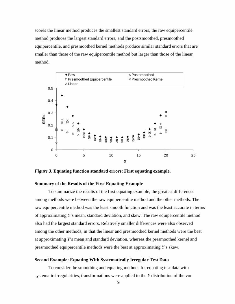
plots the five methods’ standard deviations (i.e., standard errors), showing that for most X
9
scores the linear method produces the smallest standard errors, the raw equipercentile
method produces the largest standard errors, and the postsmoothed, presmoothed
equipercentile, and presmoothed kernel methods produce similar standard errors that are
smaller than those of the raw equipercentile method but larger than those of the linear
method.
Figure 3. Equating function standard errors: First equating example.
Summary of the Results of the First Equating Example
To summarize the results of the first equating example, the greatest differences
among methods were between the raw equipercentile method and the other methods. The
raw equipercentile method was the least smooth function and was the least accurate in terms
of approximating Y’s mean, standard deviation, and skew. The raw equipercentile method
also had the largest standard errors. Relatively smaller differences were also observed
among the other methods, in that the linear and presmoothed kernel methods were the best
at approximating Y’s mean and standard deviation, whereas the presmoothed kernel and
presmoothed equipercentile methods were the best at approximating Y’s skew.
Second Example: Equating With Systematically Irregular Test Data
To consider the smoothing and equating methods for equating test data with
systematic irregularities, transformations were applied to the Y distribution of the von
0
0.1
0.2
0.3
0.4
0.5
0 5 10 15 20 25
SE
Es
X
Raw PostsmoothedPresmoothed Equipercentile Presmoothed KernelLinear
10
Davier et al. (2004) data used in the first example. These transformations include a
nonlinear arcsine transformation, rounding, and truncation of Y, transformations, which
have been described and recommended in measurement texts (Kolen, 2006; Kolen &
Brennan, 2004; Petersen, Kolen, & Hoover, 1989), and which have been considered by
several testing programs in the process of revising their scales. The arcsine transformation
is used to achieve a constant standard error of measurement across Y’s scale. The rounding
is done to make reported Y scores appealing to test users. Truncation of the transformed
Y’s largest scores is done to eliminate some of the gaps in the Y scale that would be
difficult to interpret (Kolen & Brennan, p. 354), such as would be the case when the
arcsine transformation results in increases of one score point in the untransformed Y that
correspond to increases of more than one score point in the transformed Y scale. All of
these modifications produce a transformed Y scale with integers between 30 and 55, with
some scores being impossible to achieve due to the arcsine transformation. Several
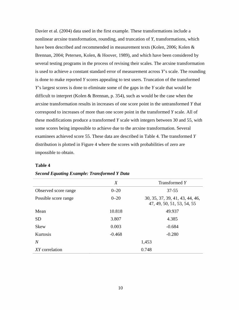
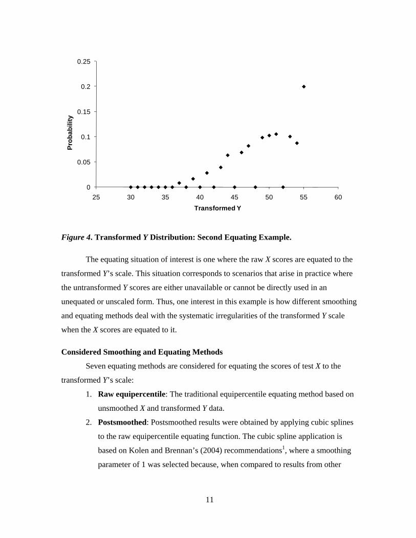
examinees achieved score 55. These data are described in Table 4. The transformed Y
distribution is plotted in Figure 4 where the scores with probabilities of zero are
impossible to obtain.
Table 4
Second Equating Example: Transformed Y Data
X Transformed Y
Observed score range 0–20 37-55
Possible score range 0–20 30, 35, 37, 39, 41, 43, 44, 46, 47, 49, 50, 51, 53, 54, 55
Mean 10.818 49.937
SD 3.807 4.385
Skew 0.003 -0.684
Kurtosis -0.468 -0.280
N 1,453
XY correlation 0.748
11
Figure 4. Transformed Y Distribution: Second Equating Example.
The equating situation of interest is one where the raw X scores are equated to the
transformed Y’s scale. This situation corresponds to scenarios that arise in practice where
the untransformed Y scores are either unavailable or cannot be directly used in an
unequated or unscaled form. Thus, one interest in this example is how different smoothing
and equating methods deal with the systematic irregularities of the transformed Y scale
when the X scores are equated to it.
Considered Smoothing and Equating Methods
Seven equating methods are considered for equating the scores of test X to the
transformed Y’s scale:
1. Raw equipercentile: The traditional equipercentile equating method based on
unsmoothed X and transformed Y data.
2. Postsmoothed: Postsmoothed results were obtained by applying cubic splines
to the raw equipercentile equating function. The cubic spline application is
based on Kolen and Brennan’s (2004) recommendations1, where a smoothing
parameter of 1 was selected because, when compared to results from other
0
0.05
0.1
0.15
0.2
0.25
25 30 35 40 45 50 55 60
Pro
ba
bil
ity
Transformed Y
12
smoothing parameter values, 1 produced equated scores with a mean, standard
deviation, and skew that were closest to those of Y.
3. – 4. Presmoothed equipercentile 1 & 2: The traditional equipercentile equating
method was applied to the X and the transformed Y data that were presmoothed
with two loglinear models. Both models fit the mean, standard deviation, and
skewness of X and transformed Y as well as the XY covariance.
The first loglinear model used to produce the presmoothed
equipercentile 1 results retained the systematic irregularities in the
transformed Y, including the impossible Y scores shown in Table 5 and
also the abnormally large frequency at the Y score of 55.
The second loglinear model used to produce the presmoothed
equipercentile 2 results ignores (and smoothes) the transformed Y’s
structural irregularities, treating all Y scores in the 30-55 score range as
if they were possible, and ignoring the abnormally large frequency at
the Y score of 55.
5. - 6. Presmoothed kernel 1 & 2: The kernel equating method was applied to the X
and the transformed Y data presmoothed with first (presmoothed kernel 1) and
second (presmoothed kernel 2) loglinear models used for the presmoothed
equipercentile 1 and 2 methods. For both applications of kernel equating, the
kernel bandwidth parameters were selected based on the recommendations of
von Davier et al. (2004), to produce continuized X and Y distributions that
matched the presmoothed and discrete X and Y distributions, but which limited
the number of modes in these distributions. The kernel bandwidths for X and
transformed Y were 0.61 and 1.35 for presmoothed kernel 1 and 0.61 and 0.44
for presmoothed kernel 2.
7. Linear: The linear equating based on the means and standard deviations of X
and Y (Table 4).
13
Table 5
Second Equating Example: Rounded Equated Scores
X X-to-Y, raw
equipercentile X-to-Y,
postsmoothed
X-to-Y, presmoothed
equipercentile 1
X-to-Y, presmoothed
equipercentile 2
X-to-Y, presmoothed
kernel 1
X-to-Y, presmoothed
kernel 2 X-to-Y, linear
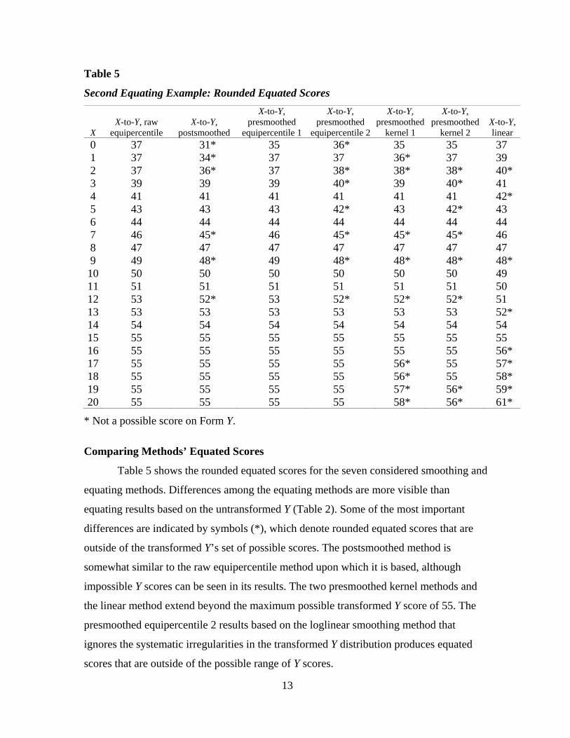
0 37 31* 35 36* 35 35 37 1 37 34* 37 37 36* 37 39 2 37 36* 37 38* 38* 38* 40* 3 39 39 39 40* 39 40* 41 4 41 41 41 41 41 41 42* 5 43 43 43 42* 43 42* 43 6 44 44 44 44 44 44 44 7 46 45* 46 45* 45* 45* 46 8 47 47 47 47 47 47 47 9 49 48* 49 48* 48* 48* 48* 10 50 50 50 50 50 50 49 11 51 51 51 51 51 51 50 12 53 52* 53 52* 52* 52* 51 13 53 53 53 53 53 53 52* 14 54 54 54 54 54 54 54 15 55 55 55 55 55 55 55 16 55 55 55 55 55 55 56* 17 55 55 55 55 56* 55 57* 18 55 55 55 55 56* 55 58* 19 55 55 55 55 57* 56* 59* 20 55 55 55 55 58* 56* 61*
* Not a possible score on Form Y.
Comparing Methods’ Equated Scores
Table 5 shows the rounded equated scores for the seven considered smoothing and
equating methods. Differences among the equating methods are more visible than
equating results based on the untransformed Y (Table 2). Some of the most important
differences are indicated by symbols (*), which denote rounded equated scores that are
outside of the transformed Y’s set of possible scores. The postsmoothed method is
somewhat similar to the raw equipercentile method upon which it is based, although
impossible Y scores can be seen in its results. The two presmoothed kernel methods and
the linear method extend beyond the maximum possible transformed Y score of 55. The
presmoothed equipercentile 2 results based on the loglinear smoothing method that
ignores the systematic irregularities in the transformed Y distribution produces equated
scores that are outside of the possible range of Y scores.
14
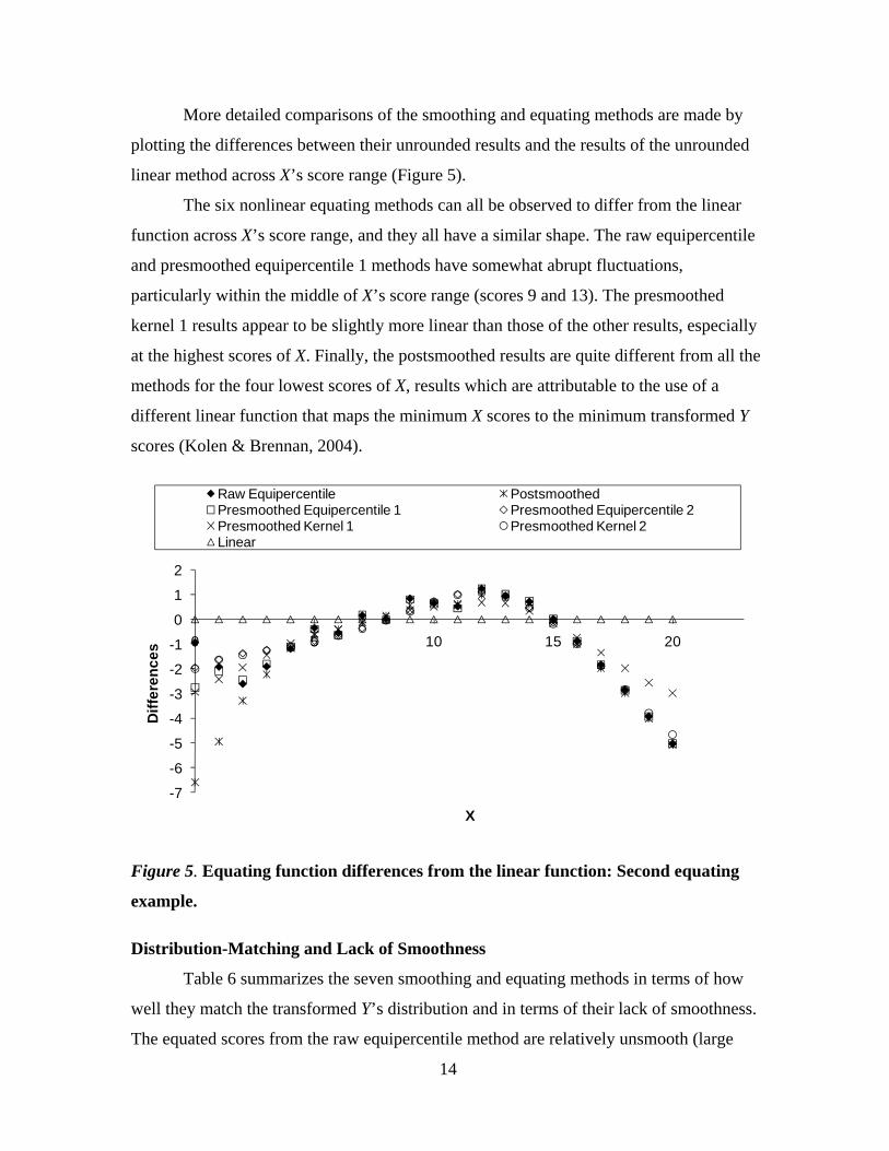
More detailed comparisons of the smoothing and equating methods are made by
plotting the differences between their unrounded results and the results of the unrounded
linear method across X’s score range (Figure 5).
The six nonlinear equating methods can all be observed to differ from the linear
function across X’s score range, and they all have a similar shape. The raw equipercentile
and presmoothed equipercentile 1 methods have somewhat abrupt fluctuations,
particularly within the middle of X’s score range (scores 9 and 13). The presmoothed
kernel 1 results appear to be slightly more linear than those of the other results, especially
at the highest scores of X. Finally, the postsmoothed results are quite different from all the
methods for the four lowest scores of X, results which are attributable to the use of a
different linear function that maps the minimum X scores to the minimum transformed Y
scores (Kolen & Brennan, 2004).
Figure 5. Equating function differences from the linear function: Second equating
example.
Distribution-Matching and Lack of Smoothness
Table 6 summarizes the seven smoothing and equating methods in terms of how
well they match the transformed Y’s distribution and in terms of their lack of smoothness.
The equated scores from the raw equipercentile method are relatively unsmooth (large
-7
-6
-5
-4
-3
-2
-1
0
1
2
0 5 10 15 20
Dif
fere
nc
es
X
Raw Equipercentile PostsmoothedPresmoothed Equipercentile 1 Presmoothed Equipercentile 2Presmoothed Kernel 1 Presmoothed Kernel 2Linear
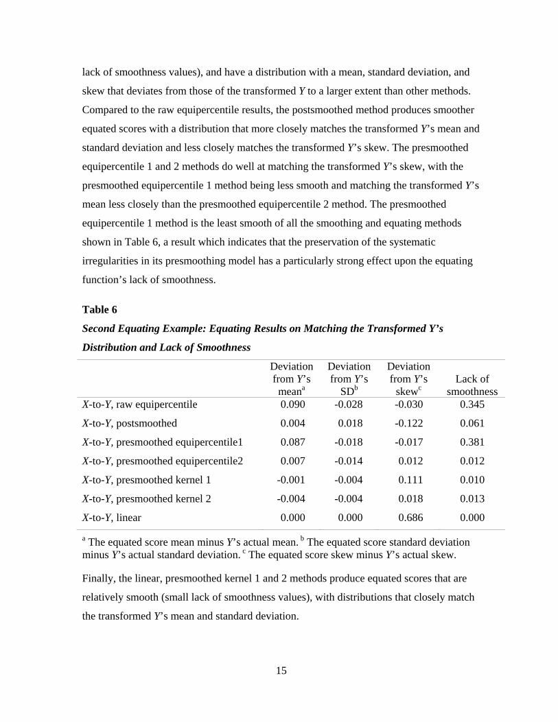
15
lack of smoothness values), and have a distribution with a mean, standard deviation, and
skew that deviates from those of the transformed Y to a larger extent than other methods.
Compared to the raw equipercentile results, the postsmoothed method produces smoother
equated scores with a distribution that more closely matches the transformed Y’s mean and
standard deviation and less closely matches the transformed Y’s skew. The presmoothed
equipercentile 1 and 2 methods do well at matching the transformed Y’s skew, with the
presmoothed equipercentile 1 method being less smooth and matching the transformed Y’s
mean less closely than the presmoothed equipercentile 2 method. The presmoothed
equipercentile 1 method is the least smooth of all the smoothing and equating methods
shown in Table 6, a result which indicates that the preservation of the systematic
irregularities in its presmoothing model has a particularly strong effect upon the equating
function’s lack of smoothness.
Table 6
Second Equating Example: Equating Results on Matching the Transformed Y’s
Distribution and Lack of Smoothness
Deviation from Y’s
meana
Deviation from Y’s
SDb
Deviation from Y’s
skewc Lack of
smoothness X-to-Y, raw equipercentile 0.090 -0.028 -0.030 0.345
X-to-Y, postsmoothed 0.004 0.018 -0.122 0.061
X-to-Y, presmoothed equipercentile1 0.087 -0.018 -0.017 0.381
X-to-Y, presmoothed equipercentile2 0.007 -0.014 0.012 0.012
X-to-Y, presmoothed kernel 1 -0.001 -0.004 0.111 0.010
X-to-Y, presmoothed kernel 2 -0.004 -0.004 0.018 0.013
X-to-Y, linear 0.000 0.000 0.686 0.000
a The equated score mean minus Y’s actual mean. b The equated score standard deviation minus Y’s actual standard deviation. c The equated score skew minus Y’s actual skew.
Finally, the linear, presmoothed kernel 1 and 2 methods produce equated scores that are
relatively smooth (small lack of smoothness values), with distributions that closely match
the transformed Y’s mean and standard deviation.

16
Standard Errors
To evaluate the seven smoothing and equating methods’ sampling variability, their
standard errors were computed using parametric bootstrap simulations (Kolen & Brennan,
2004). For the simulations, the first loglinear presmoothing model that fit the means,
standard deviations, skewness and covariance of X and Y as well as the impossible and
popular scores of the transformed Y was used as a population distribution. From this
population distribution, 1,000 samples of XY data with 1,453 observations were drawn, the X-
to-Y equating was computed using the seven methods for all 1,000 samples, and the standard
deviations of the 1,000 X-to-Y equated scores were computed at each X score. Figure 6 plots
the seven smoothing and equating methods’ standard deviations (i.e., standard errors). The
raw equipercentile and presmoothed equipercentile 1 methods’ standard errors are often
larger than those of the other methods, especially for the lowest X scores and for the X scores
of 9 and 13.
Figure 6. Equating function standard errors. Second equating example.
Other smoothing and equating methods have standard errors that are smoother and
smaller. The standard errors of the postsmoothed method appear to reflect the
irregularities of the raw equipercentile method’s standard errors (X score of 13), but in a
smoother way. Finally, the linear and presmoothed kernel 1 methods’ standard errors
appear to be most similar for the highest scores of X.
0
0.5
1
1.5
2
2.5
0 5 10 15 20
SE
Es
X
Raw Equipercentile PostsmoothedPresmoothed Equipercentile 1 Presmoothed Equipercentile 2Presmoothed Kernel 1 Presmoothed Kernel 2Linear
17
Summary of the Results of the Second Equating Example
The considered smoothing and equating methods differed in this second example
where Y was transformed to introduce systematic irregularities. The smoothing and
equating methods designed to reflect the systematic irregularities of the transformed Y
(i.e., raw equipercentile, presmoothed equipercentile 1) produced equating results and
standard errors that reflected the systematic irregularities of the transformed Y more
closely than other methods. In contrast, the linear, presmoothed kernel 1 and
postsmoothed methods introduced different forms of smoothness into the equating
function, approximating the transformed Y’s mean and standard deviation relatively
closely, approximating the transformed Y’s skew less closely, and producing some
rounded equated scores outside of the possible range of the transformed Y’s scale. The
presmoothed equipercentile 2 and presmoothed kernel 2 methods based on the smoother
loglinear model produced relatively smooth equating functions that matched the
transformed Y’s mean, standard deviation, and skew fairly closely, but reflected the
systematic irregularities and score range of the transformed Y less closely.
Discussion
Equipercentile equating functions are commonly understood to be improved when
smoothing methods are used to smooth out sampling irregularities. These beliefs about
smoothness and equating functions correspond to beliefs about population test score
distributions and equating functions, “…presumably, if very large sample sizes or the
entire population were available, score distributions and equipercentile relationships
would be reasonably smooth” (Kolen & Brennan, 2004, p. 67). The beliefs that smoothing
is usually better than not smoothing have been supported by simulation studies that have
considered population test score distributions that are smooth (Cui & Kolen, 2009; Hanson
et al., 1994), even when the smooth populations are unrealistically obtained using overly
simplistic scoring practices (Livingston, 1992, p. 3). The current study evaluated prior
suggestions from a broader perspective by considering smoothing and equating methods
for one example involving a relatively smooth population test score distribution and a
second example involving a population test score distribution with systematic
irregularities. Several smoothing and equating methods were evaluated with respect to

18
multiple equating criteria, including the extent to which the methods reflected the test
data, their smoothness, and their variability.
For the first example, the results were consistent with the overall findings of
equating texts and simulation studies. Methods such as loglinear presmoothing, kernel
equating, and cubic spline postsmoothing performed similarly in terms of producing
smooth equating functions with distributions that closely matched Y’s distribution. In
addition, the various smoothing and equating methods had smaller standard errors than
those of raw equipercentile equating. In short, when test data can be assumed to come
from relatively smooth populations, different smoothing methods can be assumed to make
similar improvements to raw equipercentile equating results.
This study’s second example involved an equating situation with a test score
distribution with systematic irregularities, a situation where the implementation of the
smoothing and equating methods was more complex and where criteria about distribution-
matching and smoothness were not consistent. The results differentiated the smoothing
and equating methods, with some methods doing especially well at matching the mean and
standard deviation of Y and at producing smooth equating functions with small and
smooth standard errors (i.e., linear, postsmoothing and kernel methods), and other
methods doing well at matching the systematic irregularities and the skew of Y (i.e.,
equipercentile methods). These results replicate prior studies (Liu et al., 2009) and expand
them by considering several smoothing and equating methods. The implication of these
results is that for systematically irregular test data, choices are required for satisfying
criteria about data-matching and smoothness when implementing smoothing and equating
methods.
Choices for using smoothing and equating methods with systematically irregular
test score distributions have only recently and partially been studied (Liu et al., 2009;
Moses & Holland, 2007; Puhan et al., 2008). Other works have approached these issues in
different ways, sometimes promoting postsmoothing with cubic splines to avoid the
complexities of systematic irregularities (Kolen, 2007, p. 53) and other times
recommending that systematic irregularities be fit and then smoothed out based on
statistical criteria (von Davier et al., 2004, p. 64). Beyond statistical criteria, pragmatic
concerns about the visibility and interpretation of equating results and the interaction of
19
equating results with scale score conversions also inform equating practice (Dorans,
Moses, & Eignor, 2010). The use of smoothing and equating methods to address
pragmatic concerns can mean that very smooth equating results may be preferred because
these results produce the most interpretable reported scores and/or because they are more
conservative ways of dealing with test data collected under less-than-perfect conditions.
The current study addresses only a few aspects of the statistical and pragmatic concerns
that inform equating practice, and uses only one set of test data. The findings for equating
tests with systematic irregularities in their distributions expand the knowledge of
smoothing and equating methods and encourage additional studies on more datasets to
clarify the use of smoothing and equating methods in equating practice.

20
References
Angoff, W. H. (1971). Scales, norms, and equivalent scores. In R. L. Thorndike (Ed.),
Educational measurement (2nd ed., pp. 508–600). Washington, DC: American
Council on Education.
de Boor, C. (2001). A practical guide to splines (Applied Mathematical Sciences,
Volume 27, 2nd ed.). New York, NY: Springer-Verlag.
Cui, Z., & Kolen, M. J. (2009). Evaluation of two new smoothing methods in equating:
The cubic B-spline presmoothing method and the direct presmoothing method.
Journal of Educational Measurement, 46(2), 135–158.
von Davier, A. A., Holland, P. W., & Thayer, D. T. (2004). The kernel method of test
equating. New York, NY: Springer-Verlag.
Dorans, N. J., Moses, T., & Eignor, D. (2010). Principles and practices of test score
equating (ETS Research Report No. RR-10-29). Princeton, NJ: ETS.
Hanson, B. A., Zeng, L., & Colton, D. (1994). A comparison of presmoothing and
postsmoothing methods in equipercentile equating (ACT Research Report 94-4).
Iowa City, IA: ACT.
Holland, P. W. (2007). A framework and history for score linking. In N. J. Dorans, M.
Pommerich, & P. W. Holland (Eds.), Linking and aligning scores and scales (pp.
5–30), New York, NY: Springer Science+Business Media, LLC.
Holland, P. W., & Thayer, D. T. (2000). Univariate and bivariate loglinear models for
discrete test score distributions. Journal of Educational and Behavioral Statistics,
25, 133–183.
Kolen, M. J. (2006). Scaling and norming. In R. L. Brennan (Ed.), Educational
measurement (4th ed., pp. 155–186). Westport, CT: Praeger Publishers.
Kolen, M. J. (2007). Data collection designs and linking procedures. In N. J. Dorans, M.
Pommerich, & P. W. Holland (Eds.), Linking and aligning scores and scales (pp.
31–55), New York, NY: Springer Science+Business Media, LLC.
Kolen, M. J., & Brennan, R. L. (2004). Test equating, scaling, and linking: Methods and
practices (2nd ed.). New York, NY: Springer-Verlag.
21
Liu, J., Moses, T., & Low, A. (2009). Evaluation of the effects of loglinear smoothing
models on equating functions in the presence of structured data irregularities
(ETS Research Report No. RR-09-22). Princeton, NJ: ETS.
Livingston, S. (1992). Small-sample equating with log-linear smoothing (ETS Research
Report No. RR-92-4). Princeton, NJ: ETS.
Livingston, S. A. (2004). Equating test scores (without IRT). Princeton, NJ: ETS.
Lord, F. M. (1965). A strong true-score theory with applications. Psychometrika, 30,
239–270.
Moses, T., & Holland, P. W. (2009). Selection strategies for univariate loglinear
smoothing models and their effect on equating function accuracy. Journal of
Educational Measurement, 46(2), 159–176.
Moses, T., & Holland, P. (2007). Kernel and traditional equipercentile equating with
degrees of presmoothing (ETS Research Report No. RR-07-15). Princeton, NJ:
ETS
Petersen, N. S., Kolen, M. J., & Hoover, H. D. (1989). Scaling, norming and equating. In
R. L. Linn (Ed.), Educational measurement (3rd ed., pp. 221–262). New York,
NY: Macmillan.
Puhan, G., von Davier, A. A., & Gupta, S. (2008). Impossible scores resulting in zero
frequencies in the anchor test: Impact on smoothing and equating (ETS Research
Report No. RR-08-10). Princeton, NJ: ETS.
Reinsch, C. H. (1967). Smoothing by spline functions, Numerische Mathematik, 10, 177–
183.
Sinharay, S., & Holland, P. W. (2009). The missing data assumptions of the
nonequivalent groups with anchor test (NEAT) design and their implications for
test equating. (ETS Research Report No. RR-09-16). Princeton, NJ: ETS.
Tong, Y., & Kolen, M. J. (2005). Assessing equating results on different equating
criteria. Applied Psychological Measurement, 29(6), 418–432.
Whittaker, E. T. (1923). On a new method of graduation. Proceedings of the Edinburgh
Mathematical Society, 41, 63–75.
Yang, W., Dorans, N. J., & Tateneni, K. (2003). Effects of sample selection on Advanced
Placement multiple-choice score to composite score linking. In N. J. Dorans (Ed.),

22
Population invariance of score linking: Theory and applications to Advanced
Placement Program examinations (ETS Research Report No. RR-03-27).
Princeton, NJ: ETS.
Zeng, L. (1995). The optimal degree of smoothing in equipercentile equating with
postsmoothing. Applied Psychological Measurement, 19(2), 177–190.
23
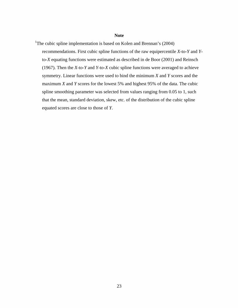
Note 1The cubic spline implementation is based on Kolen and Brennan’s (2004)
recommendations. First cubic spline functions of the raw equipercentile X-to-Y and Y-
to-X equating functions were estimated as described in de Boor (2001) and Reinsch
(1967). Then the X-to-Y and Y-to-X cubic spline functions were averaged to achieve
symmetry. Linear functions were used to bind the minimum X and Y scores and the
maximum X and Y scores for the lowest 5% and highest 95% of the data. The cubic
spline smoothing parameter was selected from values ranging from 0.05 to 1, such
that the mean, standard deviation, skew, etc. of the distribution of the cubic spline
equated scores are close to those of Y.

24
Appendix
A Measure of Smoothness for Equating Functions
Liu et al. (2009) developed a quantifiable measure of the smoothness of an
equating function from prior measures of the smoothness of cubic spline and kernel
functions (von Davier et al., 2004; Reinsch, 1967; Zeng, 1995). The common theme in
these smoothness measures is that a function’s smoothness (actually, its lack of
smoothness) can be measured in terms of the sum of its squared second derivatives. In the
context of equating functions, the lack of smoothness of an X-to-Y equating function,
( )Ye x , would be measured by computing its squared second derivatives with respect to X
and summing these across the X scores,
2( )
( )
Y
x
e xSmoothness
x. (A1)
(A1) will be zero for linear equating functions, small for smooth equating
functions, and relatively large for irregular equating functions. One problem of (A1) is
that for equipercentile ( )Ye x functions, the analytical second derivatives are zero for all X
scores, making (A1) useless for evaluating these functions’ smoothness. To make (A1)
practical for evaluating the smoothness of equipercentile equating functions, an idea from
Whittaker (1923) is borrowed, where the first derivatives of ( )Ye x with respect to X are
obtained numerically rather than analytically as the differences in the ( )Ye x scores at
one-unit intervals near the X scores of interest,
( ) ( 0.5) ( 0.5)
( ) ( 0.5) ( 0.5)
Y Y Ye x e x e x
x x x. (A2)
The idea of using numerical rather than analytical derivatives in (A2) can also be
used to obtain the second derivatives needed for (A1),
( ) ( 0.5) ( 0.5)
( ) ( 0.5) ( 0.5)
( 1) ( ) ( ) ( 0.5) .
( 1) ( ) ( ) ( 0.5)
Y Y Y
Y Y Y Y
e x e x e x
x x x
e x e x e x e x
x x x x
(A3)
Applying (A3) as a measure of an equating function’s lack of smoothness to (A1),
25
2( 1) ( ) ( ) ( 1)
( 1) ( ) ( ) ( 1)
Y Y Y Y
x
e x e x e x e xSmoothness
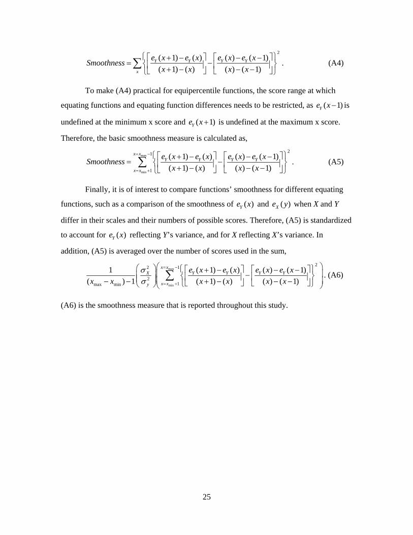
x x x x. (A4)
To make (A4) practical for equipercentile functions, the score range at which
equating functions and equating function differences needs to be restricted, as ( 1)Ye x is
undefined at the minimum x score and ( 1)Ye x is undefined at the maximum x score.
Therefore, the basic smoothness measure is calculated as,
max
min
21
1
( 1) ( ) ( ) ( 1)
( 1) ( ) ( ) ( 1)
x xY Y Y Y
x x
e x e x e x e xSmoothness
x x x x. (A5)
Finally, it is of interest to compare functions’ smoothness for different equating
functions, such as a comparison of the smoothness of ( )Ye x and ( )Xe y when X and Y
differ in their scales and their numbers of possible scores. Therefore, (A5) is standardized
to account for ( )Ye x reflecting Y’s variance, and for X reflecting X’s variance. In
addition, (A5) is averaged over the number of scores used in the sum,
max
min
212
21max min
( 1) ( ) ( ) ( 1)1
( ) 1 ( 1) ( ) ( ) ( 1)
x xX Y Y Y Y
x xy
e x e x e x e x
x x x x x x
. (A6)
(A6) is the smoothness measure that is reported throughout this study.


