Smooth Interpolation of Orientations Gregory M. Nielson This is a slightly modified version of an earlier paper: Models and Techniques in Computer Animation, (Magnenat Thalmann N and Thalmann D, eds), Springer-Verlag, Tokyo, 1993, pp.75-93. ABSTRACT The problem of smoothly interpolating between a given sequence of orientations is discussed. Methods of representing orientations are described and some of the more interesting and useful properties of orientation matrices, SO(3), are covered. It is shown how quaternions relate to this problem and several methods of smoothly interpolating quaternions are presented. KEYWORDS Animation, Interpolation, Orientations, Rotations, Quaternions 1. INTRODUCTION It is a fundamental problem of computer animation and other computer simulations involving the dynamics of rigid bodies to be able to smoothly interpolate between a sequence of positions and orientations. In the past, traditional animation required animators to produce a large number of frame sequences to simulate a moving scene. In key frame animation, only a relatively small number of key frames have to be specified and a computer algorithm can compute the frames in between. A fly-through consisting of the path and orientation of a camera through a scene can be specified as a relatively sparse sequence of positions and orientations and then an interpolation technique can be used to compute intermediate position and orientations which are used to render the scene. The path of rigid bodies animated through space can be handled in much the same manner. Often, techniques for solving these problems separate the position and orientation. Whether or not this is a wise move, we do not discuss here. Interpolating smoothly to positions in space is relatively easy to accomplish with any number of the rich variety of curve techniques that are available today. Interpolating smoothly to a sequence of orientations is currently a much more interesting problem. What makes it interesting is the mathematics behind the problem and the fact that many commercial systems don't work very well. This is most likely due to the fact that these systems use simple techniques which are basically flawed for this application. In this paper we discuss a variety of methods for solving the problem of smoothly interpolating a sequence of orientations. In the remaining portion of this section, we discuss two methods for representing orientations: Eulerian angles and orientation matrices. We elaborate on orientation matrices and establish some useful and interesting properties about them. In the next section, we move to the actual problem of developing a method for smoothly interpolating orientation matrices. This requires some means of parameterizing orientation matrices. Quaternions are introduced and several methods based upon quaternions are described and compared. At the end of this section we discuss "knot spacing" which is an often overlooked and important aspect of this problem.

1.1 The Representation of Orientations In order to obtain a solution to the problem we have described, we need some mathematical means of representing orientations. One method which has a long history with flight control and aerospace is the use of Eulerian angles. For this method, three angles of rotation, α, β and γ are specified. These angles are often called pitch, roll and yaw. A point, P, is mapped to a point, P', by the successive application of these rotations about the coordinate axes; P' = P Rx(α)Ry(β)Rz(γ)

= P

1 0 0

0 cos(α) sin(α) 0 -sin(α) cos(α)

cos(β) 0 -sin(β)

0 1 0 sin(β) 0 cos(β)

cos(γ) sin(γ) 0

-sin(γ) cos(γ) 0 0 0 1

. (1)

In any system, there are two places where this representation may be used. First it may be used as a means of specifying the orientation and secondly, it may be used to represent the orientation and serve as a basis for the interpolation scheme. In the first use, it serves to establish a certain model of interaction whereby the user places an object into a certain orientation by "rotating" it into position. The rotation being about the successive coordinate axes and applied in a predetermined order. Without modifications, this method of specifying orientations can have some problems. We will discuss one such potential problem. Usually when Eulerian angles are used in the interactive specification of orientation, they are applied in a "relative" manner. First a rotation about one of the coordinate axes is applied. This establishes a new coordinate system and subsequent rotation are performed relative to this new coordinate system. In terms of rotations about the original coordinate axes, we have the three relative rotations Rx(α) Ry'(β) = Rx(-α)Ry(β)Rx(α) Rz"(γ) = Rx(-α)Ry(-β)Rz(γ)Ry(β)Rx(α) The composite operation of these three relative operators is just the same as the operators about the original coordinate axis, but in reverse order; i.e. Rx(α)Ry'(β)Rz"(γ) = Rz(γ)Ry(β)Rx(α) This is no surprise since we are simply rotating the axes rather than the object. Even though the final composite form is rich enough to represent any orientation, because of the manner in which they are applied, there is a problem. An example will serve to point this out. Let α = π/2 = β then Rz"(γ) = = which is the same as Rx(γ) and so we called "gimbal lock".

0 1 0

0 0 0 1

1

0

0 0 1 0

)

1 0 0

cos(γ)

have "l

1 0 0 ) 0 0

cos(γ) sin(γ)

- sin(γ

0 1 0 1 0

cos(γ) sin(γ)

cos(γ)

0

- sin(γ

0

ost one degree of rotation". This is sometimes

x"

y"z"

γx

y

z

α

x'

y'

z'

β

Fig. 1 Successive application of Eulerian angles Problems can also arise in the second use of Eulerian angles. For example some orientations do not lead to uniquely determined representations. A specific example is given by an orientation where the x-axis is oriented in the direction (0, 0, -1), the y-axis is oriented in the direction (s, c, 0) and z-axis is oriented in the direction (c, -s, 0). For this example, the values c and s are arbitrary except that c2 + s2 = 1. Factoring this orientation into Eulerian angles leads to the conditions

0 0 -1s c 0c -s 0

= Rx(α)Ry(β)Rz(γ).

Multiplying both sides of this equation by Rx(-α) from the left and Rz(-γ) from the right and comparing elements we are lead to the requirement that β must be π/2. The remaining constraints are

0 0 -1

sin(α−γ) cos(α−γ) 0 cos(α−γ) -sin(α−γ) 0

=

0 0 -1s c 0c -s 0

which are not sufficient to uniquely determine α and γ and this is the problem.

x

y

z

(0,0,-1)

(s,c,0)

(c,-s,0)

+1

-1

Fig. 2 Problem example Fig. 3 Characteristic polynomial

A great many systems (in fact, most of the commercial animation systems we are aware of) use the Eulerian angle type of representation of orientations. Of course, there are a number of variations in the way they are implemented, but they all suffer from problems which can often be traced back to the flaws we have just identified. Also, there is the problem of how to interpolate in between. A large positive angle is close to (or the same as) a small negative angle and also close to a small positive angle and so it is mandatory to have some type of "periodic" interpolation scheme which computes the intermediate values independently of how they are represented. Conventional interpolation methods applied in a straightforward manner to α, β and γ simply do not work.

Another method of representation is to simply write the new coordinate of the oriented object in terms of a global coordinate system. We let O1 = ( o11, o12, o13 ) be the new orientation of the x-axis, O2 = ( o21, o22, o23 ) be the new orientation of the y-axis and O3 = ( o31, o32, o33 ) the new orientation of the z-axis. If P is a point on the object in the original coordinate system, and P' is a point on the new oriented object then

P' = PO and

O =

o11 o12 o13

o21 o22 o23 o31 o32 o33

. (2)

The image of the original axes provides a frame which is also an orthonormal basis and so (Oi, Oj) = δij which is the same as writing

OOt = I

where I is the 3 by 3 identity matrix. In general a matrix with this property is called orthogonal. Let |A| denote the determinant of A and recall that |AB| = |A| |B| and |At| = |A|. From this, we can deduce that if Q is orthogonal then |QQt| = |Q|2 = 1 and so the determinant of an orthogonal matrix is either +1 or -1. Since the coordinate system remains right handed after orientation, we have that O3 = O1 x O2. Using this along with the fact that |O| = (O1 x O2, O3) allows the conclusion that |O| = 1. Both of the properties of being orthogonal and having a unit determinant are preserved under matrix multiplication. This group of orientation matrices (orthogonal matrices with determinate 1) has received a great deal of attention in the past. One of the main reasons, of course, is due to its ability to represent orientations of rigid bodies as we have established here. In the mathematical literature, this collection of matrices is often denoted by SO(3) which is a Lie group and as such has the structure of both a differential manifold and an algebraic group. 1.2 Properties of Orientation Matrices (SO(3)) There are some very interesting properties about SO(3) which are worthy of note. The first is the connection to rotations. Embedded in the terminology of the Eulerian angle approach to representing orientations, is the idea of rotations, but the SO(3) method of representation is simply direct and has no mind as to how the object got where it is, only that it is there. Nevertheless there is a strong connection between elements of SO(3) and rotation matrices which was first noted in the late eighteenth century by Euler.

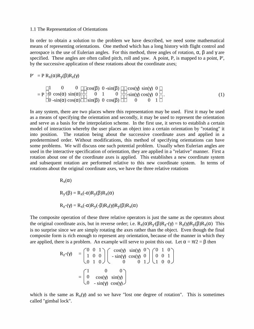
Theorem: If OOt = I and |O| = 1, then O represents a rotation. The axis of rotation is the eigenvector of O associated with the eigenvalue 1. The angle of rotation, θ, satisfies 1 + 2cos(θ) = tr(O) (3) where tr(O) denotes the trace (sum of diagonal elements). In less formal terms, this theorem states that no matter how we arrive at a particular orientation, whether it be by a sequence of rotations (however long) or even by a sequence (even number) of reflections across arbitrary planes, we can arrive at this very same orientation by one single rotation. It is interesting and instructive to go through some of the steps of the proof of this theorem. We want to first show that O has 1 as an eigenvalue. The first thing to note in this regard is that

(λu,λu) = |λ|2(u,u) = (uO,uO) = uO(uO)t = uOOtut = (u,u) and so any eigenvalue must satisfy |λ| = 1. A direct computation will show that the characteristic polynomial can be written as p(λ) = |λI-O| = λ3 - (tr(O)λ2 + k(O)λ - 1 (4) where

k(O) = o22o33 + o11o33 + o11o22 - o31o13 - o21o12 - o32o23. Since P(0) = -1 and the coefficient of the leading term λ3 is positive, we know that P must have at least one positive root and since this root must satisfy |λ| = 1, we know that λ= 1 must be an eigenvalue. See Fig. 3 above. The remaining two roots must be complex conjugates which have magnitude 1. Let u denote an eigenvalue associated with the eigenvalue 1 so that u = uO. Let P be an arbitrary point and P' = PO. We want to show that P' remains in the plane which contains P and has u as a normal. P can be factored into the sum of a component along u and one perpendicular to u; namely P = (u,P)u + [ P - (u,P)u]. See Fig. 4 below. Now P' = PO = (u,P)u + [P - (u,P)u]O and so P' is in this same plane since the second term in this sum is a vector that is perpendicular to u. This is because ([P - (u,P)u]O,u) = POut - PutuOut = 0. Also, it is not difficult to show that the angle, θ, between [P - (u,P)u]O and [P-(u,P)u] is independent of P and must satisfy tr(O) = 1 + 2 cos(θ). As we noted earlier, all orthogonal matrices have a determinate that is either +1 or -1. If it is +1, then it is an orientation matrix and can be viewed as a single rotation about its eigenvector which associates with the eigenvalue 1. If the determinant of the orthogonal matrix Q is -1 then an argument similar to the one above involving the characteristic polynomial can be used to show that Q has -1 as an eigenvalue. If v, of length one, is an associate eigenvector then we can factor Q as

Q = R[I - 2vtv] or Q = [I - 2vtv]S where R = Q[I-2vtv] is now orthogonal with determinant +1 and with associate eigenvector v. S has the same properties and so both R and S represent rotations about v. In general, the matrix

I - 2wtw,

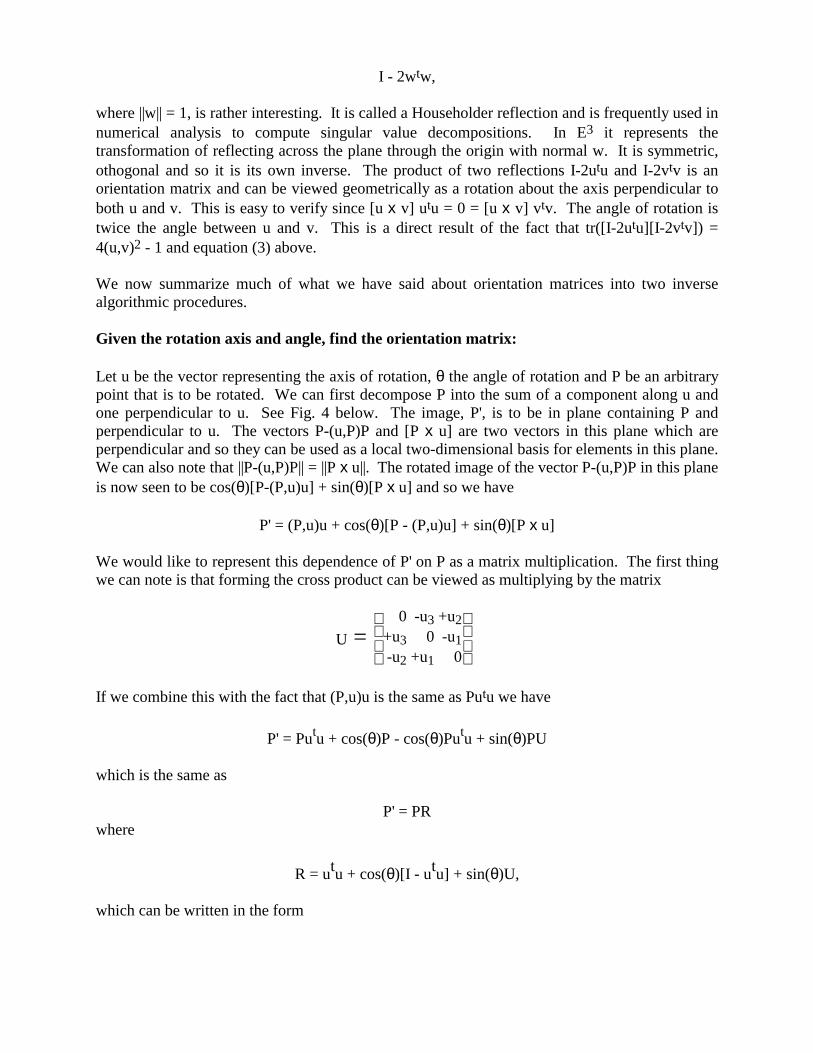
where ||w|| = 1, is rather interesting. It is called a Householder reflection and is frequently used in numerical analysis to compute singular value decompositions. In E3 it represents the transformation of reflecting across the plane through the origin with normal w. It is symmetric, othogonal and so it is its own inverse. The product of two reflections I-2utu and I-2vtv is an orientation matrix and can be viewed geometrically as a rotation about the axis perpendicular to both u and v. This is easy to verify since [u x v] utu = 0 = [u x v] vtv. The angle of rotation is twice the angle between u and v. This is a direct result of the fact that tr([I-2utu][I-2vtv]) = 4(u,v)2 - 1 and equation (3) above. We now summarize much of what we have said about orientation matrices into two inverse algorithmic procedures. Given the rotation axis and angle, find the orientation matrix: Let u be the vector representing the axis of rotation, θ the angle of rotation and P be an arbitrary point that is to be rotated. We can first decompose P into the sum of a component along u and one perpendicular to u. See Fig. 4 below. The image, P', is to be in plane containing P and perpendicular to u. The vectors P-(u,P)P and [P x u] are two vectors in this plane which are perpendicular and so they can be used as a local two-dimensional basis for elements in this plane. We can also note that ||P-(u,P)P|| = ||P x u||. The rotated image of the vector P-(u,P)P in this plane is now seen to be cos(θ)[P-(P,u)u] + sin(θ)[P x u] and so we have

P' = (P,u)u + cos(θ)[P - (P,u)u] + sin(θ)[P x u] We would like to represent this dependence of P' on P as a matrix multiplication. The first thing we can note is that forming the cross product can be viewed as multiplying by the matrix

U =

0 -u3 +u2

+u3 0 -u1 -u2 +u1 0

If we combine this with the fact that (P,u)u is the same as Putu we have

P' = Putu + cos(θ)P - cos(θ)Putu + sin(θ)PU which is the same as

P' = PR where

R = utu + cos(θ)[I - utu] + sin(θ)U, which can be written in the form

R=

u2

1+cos(θ)(1-u21) (1-cos(θ))u1u2-sin(θ)u3 (1-cos(θ))u3u1+sin(θ)u2

(1-cos(θ))u1u2+sin(θ)u3 u22+cos(θ)(1-u2

2) (1-cos(θ))u2u3-sin(θ)u1

(1-cos(θ))u3u1-sin(θ)u2(1-cos(θ))u2u3+sin(θ)u1 u23+cos(θ)(1-u2

3)

(5)

P

(u,P)u

P - (u,P)u

P'

θ

Fig. 4 Rotation of orientation matrix A quite different approach (see Fillmore 1984) to this same result is a consequence of the following facts which hold for an arbitrary antisymmetric matrix

S =

0 -s3 +s2

+s3 0 -s1 -s2 +s1 0

.

1) eS = I + S + S2

2 + S3

3! + is orthogonal, since St = -S.

2) |eS| = 1, since |eA| = etr(A) for any matrix and tr(S) = 0 3) s = (s1, s2, s3) is an eigenvector of eS since sS = 0. 4) tr(eS) = 1 + 2cos||s||, since tr(S2) = -||s||2. Using the identities S2n = (-1)n-1||s||2n-1S2, S2n+1 = (-1)n||s||2nS, the infinite exponential expansion reduces to

eS = I + sin||s||

||s|| S+ 1-cos||s||

||s||2 S2 .

Combining this, we have the alternate representation of a rotation about u an angle θ, R = I + sin(θ)U + (1-cos(θ))U2 (6) Given an orientation matrix, find rotation axis and angle:

There are several ways to obtain the eigenvector which is the axis of rotation. For example, it can be taken as a multiple of any row of

R + Rt - (tr(R) -1)I.

The angle of rotation, θ, can be computed from the identity tr(R) = 1 + 2cos(θ). (7) We should mention that this process of computing the axis and angle of rotation from the orientation matrix is very closely related to the conversion algorithm for quaternions covered below. 2. SMOOTH INTERPOLATION OF ORIENTATION MATRICES We now discuss the problem of interpolating a sequence of orientation matrices. We assume we have a sequence of orientation matrices, Ri, i = 1, . . . , n and an associated sequence of parameter (time) values ti, i = 1, . . . , n. We wish to construct a smooth matrix valued function R(t) such that R(t) is an orientation matrix for all t and R(ti) = Ri, i = 1, . . . , n. An orientation matrix has 9 entries and we could easily compute a scalar valued interpolant for each of these nine entries, but this will clearly not work for there is nothing to guarantee that the intermediate matrices would continue to be an orientation matrix. The columns and rows must remain of unit length and they must be mutually orthogonal. So, what can we use for the data of the interpolation so that we are guaranteed to always get an orientation matrix? What we need is to know how many degrees of freedom or free parameters there are involved in an arbitrary orientation matrix. In other words, we need some type of parameterization of orientation matrices. The results from above (see equation (5)) on the relationship to rotation matrices gives us some indications. Roughly speaking, it appears that they are three independent free parameters: two for the axis of rotation (it is normalized) and one for the angle of rotation. But the situation is more complicated and subtle than that. It is true that SO(3) is locally equivalent to E3; that is, it is a three dimensional manifold. Euler established this in the late 18th century. But SO(3) is not the same as E3, it is a different 3D manifold. Just as the sphere or the torus are two dimensional manifolds which are not equivalent to E2, SO(3) is a 3D manifold different from E3. While it is easy for us to comprehend what a torus or a sphere "looks like" when they are in E3, it is very difficult to imagine what SO(3) "looks like" in E4. In fact, it turns out that SO(3) can not be embedded in E4. Hopf (1940) has shown the if we wish to embed SO(3) in Ek, then k must be greater than or equal to 5. (Whitney's embedding theorem gives an upper bound on k to be 2(3)+1 = 7.) Even though SO(3) can not be embedded in E4, there is a mapping between SO(3) and the sphere in E4 which is 1 to 2. That is, two points on the unit sphere in E4 correspond to one point in SO(3). This association is the quaternion mapping and has proven to be very useful in this context. The fact that it is not an embedding (1 to 1) presents some special problems that must be dealt with carefully. 2.1 Quaternions Based upon the same notation as in equation (5), we make the associations

qx = u1 sin(θ2 ), qy = u2 sin(

θ2 ), qz = u3 sin(

θ2 ), and qw = cos(

θ2 ) (8)

then R takes the form

R =

1-2qy

2-2qz

2 2qxqy+2qwqz 2qxqz-2qwqy

2qxqy-2qwqz 1-2qx2-2qz

2 2qyqz+2qwqx

2qxqz+2qwqy 2qyqz-2qwqx 1-2qx2-2qy

2 = R(q) . (9)

The four-tuple, q = (qx, qy, qz, qw) is a quaternion which has the property that

qx 2 + qy

2 + qz

2 + qw

2 = 1.

The rule for multiplying two quaternions is qr = (qwrx - qzry + qyrz + qxrw, qzrx + qwry - qxrz + qyrw, -qyrx + qxry + qwrz + qzrw, -qxrx - qyry + qzrz + qwrw ) so that R(qr) = R(q)R(r). The multiplicative inverse of q is denoted by q-1 and is given by

q-1 = (-qx, -qy, -qz, qw) The use of quaternions in the representation of rigid body motion has been discussed by many authors. Hamilton (1843) introduced quaternions and soon after Cayley (1845) noted the connection to rotation matrices. More recent discussion on this topic as it relates to practical issues for the computer generation and control of rigid bodies has been given by Brady (1982), Brekke (1978), Goldstein (1980), Schut (1960), Thompson (1958, 1959), Wittenburg (1977), Horn (1987), Ickes (1970), Kane, Likins and Levinson (1983), Robinsion (1958), Sunkel (1976), Stuelpnagle (1964), Taylor (1982) and Wertz (1978). The use of quaternions gives rise to a general approach to animating orientations which has three steps:

1) The quaternions

qi = q(Ri) , i = 1, . . . , n

associated with each orientation are computed. 2) A curve q(t), which lies on the four dimensional unit sphere, is constructed so that q(ti) = qi , i = 1, . . . , n. 3) The inverse mapping, R = R(q) which takes a quaternion back to an associated rotation

matrix is then used to define the animation function,

R(t) = R(q)(t),

which has the required interpolation properties R(ti) = R(q)(ti) = q(ti) = qi, i = 1, . . . , n.

Previously (see Nielson and Heiland (1992)) we used a certain conversion algorithm which has been proposed in the literature, but we now prefer the following: Algorithm(q ← q(R))

Solve for the largest in magnitude of qx, qy, qz, and qw from one of the equations

4q2w = 1 + r11 + r22 + r33

4q2x = 1 + r11 - r22 - r33

4q2y = 1 - r11 + r22 - r33

4q2z = 1 - r11 - r22 + r33

then solve for the remaining three values from three of the following equations:

4qwqx = r23 - r32, 4qwqy = r31 - r13 4qwqz = r12 - r21, 4qxqy = r12 + r21

4qyqz = r23 + r32, 4qzqx = r31 + r13 . As was mentioned earlier, the mapping from SO(3) to the quaternions is 1 to 2 which shows up here in the choice of positive or negative square root. In general, choosing the proper branch of this mapping could present a problem, but for our application we have the context of a sequence of values to aid us in our choice. For the first matrix, we take the quaternion produced by the above algorithm using the positive square root, then for subsequent orientations, we take either q or -q depending upon which one is closer (in geodesic distance on the unit 4D sphere) to the previously chosen quaternion. We would like to point out an interesting property of quaternions. In some since the quaternions are richer than the elements of SO(3) as far as representing rotations. For example, elements of SO(3) can not distinguish between an orientation which results from zero rotation about an axis and one which results from a 360 degree rotation about the same axis, but the quaternions can make this distinction. The element of SO(3) which represents zero rotation is the identity matrix and the rotation of 360 degrees is the same matrix. For quaternions, (0, 0, 0, 1) represents rotation of zero degrees and (0, 0, 0, -1) represent rotation of 360 degrees. Now if we want to interpolate in between these two values we can do it with quaternions. (Interpolating between two identical orientation matrices does nothing.) Say the axis of rotation is (a,b,c) then

q(t) = (a 2t-4t2 , b 2t-4t2 , c 2t-4t2 , 2t-1), 0 ≤ t ≤ 1 will spin entirely around this axis. Repeating this will give any number of spins around a specified axis. 2.2 Methods for Smoothly Interpolating Quaternions In this section, we discuss several methods for determining a curve, c(t), which interpolates to a given sequence of quarternions, qi , i = 1, . . . , n. We assume that knot values ti , i = 1, . . . , n have been specified so we have the interpolation requirements

c(ti) = qi , i = 1, . . . , n

From the discussion above, we know that it is important that c(t) have the property that ||c(t)||= 1 for all values of t. It is this constraint that makes this whole problem interesting. Geometrically, this constraint is equivalent to restricting c(t) to be on a unit sphere and the figures of this section might give the impression that the curve methods we are describing are only for a two dimensional sphere in E3, but the figures are only a guide and it should be kept in mind that the curve schemes are being defined for the space of quaternions. Normalized Cubic Spline and Related Methods: A very simple approach is to choose c(t) to be a cubic interpolating spline in E4. The basic problem is that there is nothing to guarantee that the spline will remain on the unit sphere inbetween interpolation points. If we assume that ||c(t)|| ≠ 0, we can force this condition by simply using the normalized spline,

C(t) = c(t)

||c(t)|| .

This is really a rather inelegant way to solve the problem, but it does have the potential to give a C2 curve which interpolates the data and remains on the unit sphere. The basic drawback to this approach is the potential occurrence of cusps or tight kinks which result form the normalization. This possibility is illustrate in the case of E3 in Fig. 5.

q i

M1

M2

Mi+1

Mi

qi+1

q2

Fig. 5 Kinks and loops Fig. 6 Nielson/Shieh Circle Spline One way to pull out the kinks is to use the 4D version of the ν-spline (see Nielson 1986). Similar to the normal cubic spline, the ν-spline is a composite curve made up of cubic segments. In addition there is associated with each interpolation point a tension parameter, νi, which can be used to tighten the curve in order to remove any unwanted inflection points, loops or kinks. If all tension values are zero, then the ν-spline simply reduces to the standard cubic spline. It is very easy to compute a ν-spline; only a tridiagonal system of equations must be solved. While it is

true for non zero tension values that the ν-spline is not C2 at the joining points, it is G2. The definition of a G2 curve means that it can be reparameterized so as to be C2 without changing the shape of the curve. In some respects this means that the curve is as smooth as a C2 to begin with. Not only do the tension values add the ability to pull the kinks out of the interpolating curve, they also add some interesting and useful parameters to affect the "shape" and "speed" of the animation. The main drawback is the lack of any algorithm for automatically selecting the tension values. Of course this is not a drawback if one has the ability and inclination to interactively edit and "design" the interpolating curve. As usual, there are trade-offs. The Nielson/Shieh Circle Method: The interpolation curve used for this method consists of a collection of rational quadratic curves constrained to lie on the unit sphere in E4 and joined so as to have C1 continuity. See Fig. 6 above. It is easy to verify that if (Mi-qi, qi) = 0, (Mi-qi+1, qi+1) = 0, (10) and

wi = 1-(qi,qi+1)2(||Mi||2-1) ,

then

ci(t) = qi(1-t)2 + wiMi2(1-t)t + qi+1t2

(1-t)2 + wi2(1-t)t + t2

has the properties ci(0) = qi, ci(1)= qi+1, c'i(0) = 2wi(Mi-qi), c'i(1) = 2wi(qi+1-Mi) (11) and

||ci(t)|| = 1 . In order to have a composite curve with C1 continuity, it must be the case the qi lies on the line segment joining Mi and Mi+1, i = 1, . . . , n. This condition along with (10) uniquely determines all the Mi's once M1 has been selected.

for i = 2, . . . , n-1

Mi = qi[1-(qi+1,Mi-1)] + Mi-1[(qi, qi+1)-1]

(qi+1, qi-Mi-1) (12)

The only conditions on M1 are that (q1, M1) = 1 = (q2, M1). The value of M1 can have considerable effect on the overall shape of the composite curve and it is not easy to select an overall "good" value for M1. We have found that a rather reasonable criterion is to select M1 so as to minimize the overall length of the NURB polygon which defines the curve or some other similar quantity. That is, M1 is selected so that

P(M1) = ||M1-q1|| + ∑i=1

n-2 ||Mi+1-Mi|| + ||Mn-1 - qn|| (13)

or, for example,

P(M1) = ∑i=1

n-1 ||ci(1/2) - Mi||2 (14)

is a minimum. We should point out that the composite curve is not really C1 at this point. It is G1. The tangents from the left and right at qi are in the same direction, but they do not match in magnitude. It is possible to reparameterize each segment with a rational linear function of the form

t = s

ai +(1-ai)s (15)

so that each curve segment remains a rational quadratic and the overall curve is C1. This reparameterization does not change the shape (graph) of the composite curve, but it does change the "speed" with which it is spanned out by the parameter and so if we use this method for animating orientations, the reparameterization does not affect the orientations that are visited between key frames, but it does affect the speed at which these orientations are visited. In our view this reparameterization improves the "smoothness" of the animation. Another method based upon circles is the method of Kim and Nam (1992) which uses a "hypercircle" (the intersection of a hyperplane and a sphere in E4) to interpolate three quaternions qi-1, qi and qi+1. These circles are then blended together in a manner similar to Overhauser curves to yield an overall C1 method. Spherical Bernstein/Bezier Methods: There are a number of methods that are based upon a spherical analog of the the de Casteljau algorithm for defining a Bernstein/Bezier curve. Usually low order curves analogous to quadratics or cubics are joined together so as to obtain an composite interpolating curve that is C1. The de Casteljau algorithm for computing points on a Bernstein/Bezier curve is based upon successive use of the simple and basic operation of linear interpolation. In the cubic case, the B/B curve with control points b0, b1, b2 and b3 is evaluated at the argument t by performing the following sequence of linear interpolations. The last value b3

3(t) is the value on the curve for the parameter value t. b1

1(t) = (1-t)b0 + tb1, b12(t) = (1-t)b1 + tb2, b1

3(t) = (1-t)b2 + tb3

b22(t) = (1-t)b1

1(t) + tb12(t) , b2

3(t) = (1-t)b12(t) + tb1

3(t)

b33(t) = (1-t)b2

2(t) + tb23(t)

There is a direct analog of this algorithm to case where the control points are on a unit sphere. Rather than linear interpolation, geodesic interpolation on the sphere is used. Given two points P0, P1, the parametric representation of the geodesic joining them is given by

G[P0,P1](t) = P0sin(1-t)θ + P1sin(tθ)

sin(θ) (16)

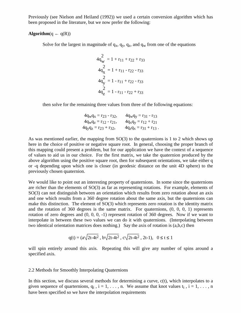
where cos(θ) = (P0, P1). We should point out that this formula also holds for the geodesic on the 3D sphere in E4. The geometric version of the de Casteljau algorirhtm in the case of four points on a sphere is illustrated in Fig. 7.

b1

b2

b21

b3

3

b22

b0

b11

b3

q i

M2

Mi+1

Mi

qi+1

q2

Fig. 7 Spherical de Casteljau Fig. 8 Spherical Quad. B-Spline In a more general situation, a formal definition of a spherical B/B curve with control point si , i = 1, . . . , n is taken to be sn

n = B[so, s1, . . . , sn](t) (17) where

ski (t) = G[sk-1

i-1 , sk-1i ](t)

and s0

i = si, i = 1, . . . , n. It is not difficult to verify that sn

n(0) = so, snn(1) = sn,

dsn

ndt (0) = ncos-1(s0,s1)

s0 x s1 x s0||s0 x s1 x s0||

and

dsnn

dt (1) = ncos-1(sn,sn-1)sn x sn-1 x sn

||sn x sn-1 x sn||

The Spherical Quadratic B-spline Method: This method is similar in many respects to the Nielson/Shieh circle method. See Fig. 8 above. Between qi and qi+1 the curve is defined by a second order spherical B/B curve B[qi, Mi, qi+1](t) = Bi(t) . (18) In this case, the shoulder points, Mi, are on the sphere and given M1 we can compute the remaining ones by Mi+1 = G[Mi, qi+1](2), i = 1, . . . , n (19) Similar to the Nielson/Shieh circle method, the overall shape of the curve is affected considerably by the choice of the first shoulder point M1. Again, a reasonable choice is to select M1 so that

P(M1) = (M1,q1) + ∑i=1

n-1 (Mi+1,Mi) + (Mn-1,qn) (20)

or

P(M1) = ∑i=1

n-1 |(Bi(1/2),Mi)|2 (21)

is a minimum. Regardless of how M1 is chosen, this method is global in the sense that changing any of the orientations will effect the animation everywhere. From some points of view, this could be a desirable property depending upon the extent of the influence. One way to avoid having a global interpolating curve and to still have C1 continuity is to use a "higher order" curve segments based upon four control points. These are the analogs of cubic curves given by B[qi ,Ri ,Li+1 ,qi+1](t), 0 ≤ t ≤ 1, i = 1, . . . , n-1 (22) where we denote the inner Bezier points between qi-1 and qi as Ri-1 and Li. See Fig. 9 below. As long as we choose the L's and R's so that

G[Li, Ri](1/2) = qi then we will be guaranteed to have a C1 curve. One approach is to take

Ri = G[G[qi-1, qi](2),qi+1](1/2)

Li = G[Ri, qi](2)

Shoemake (1985) states "For the numerically knowledgeable, this construction approximates the derivative at points of a sampled function by averaging the central difference of the sample sequence". The Catmull/Rom spline is also based upon estimates of derivatives based upon central differences. These ideas can be mapped to the present context by the following choice of inner Bezier points

Ri = G(qi, qi+1q-1

i-1 qi](1/6)

Li = G[qi+1,qiq-1i+2 qi+1](1/6) .

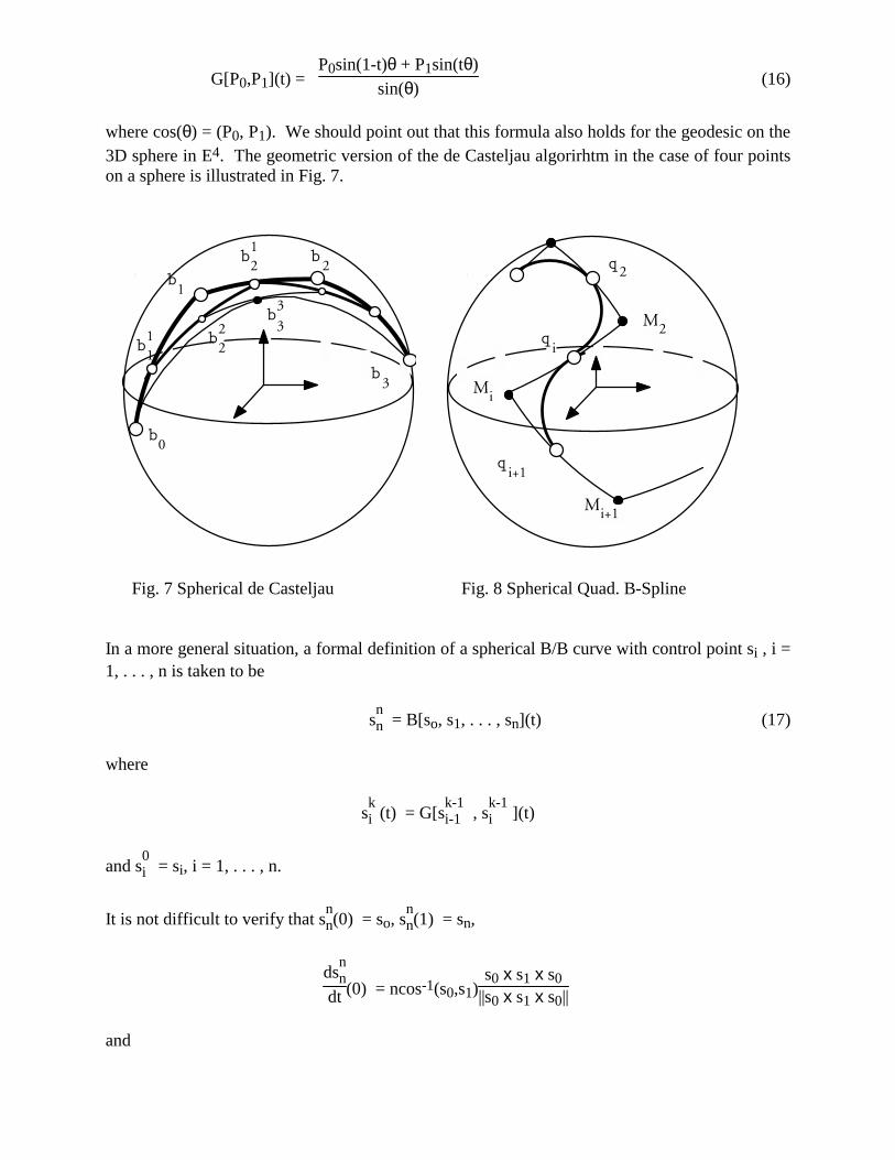
Hanson (private communication) has shown that this choice is the same as that of Schlag (1992). The Nielson/Heiland Spherical B-spline Method: One the smoothest methods of this type that we have observed is a method proposed by Nielson and Heiland (1992) which is based upon "spherical B-splines". There is a well known geometric construction of cubic B-splines that is based solely upon linear interpolation. This construction is illustrated in Fig. 9, where the Di's are the given control points. The inner Bezier points of the cubic segment are computed at 1/3 and 2/3 of the distance between the B-spline control points. Nielson and Heiland adapt this construction to a sphere by replacing linear interpolation with geodesic interpolation. B-splines do not interpolate to their data, they only approximate it. For the application of animating orientations, it is important to be able to construct a curve that interpolates the data. In much the same way that B-splines can be used as a basis for constructing a cubic interpolating spline, Nielson and Heiland use the spherical B-spline to find an interpolating curve which is composed of joining together segments of third order spherical B/B curves. In the conventional case, a tridiagonal, linear system of equations must be solved. In the spherical case, a system with the same sparsity (each equation has only three unknowns) must be solved, but it is no longer linear. They use an iterative method to solve it: Choose an initial approximation to the spherical B-spline control points, D(0)

i , i = 1, . . . , n. Then iterate until convergence with: D1 = q1

Di = βiqi - αi-1(1

3)Di-1 - αi(13)Di+1

αi-1(23) + αi(

23)

, i = 2, . . . , n-1 (22)

Dn = qn where

βi = sin(ϕi)

sin(ϕi2 )

, cos(ϕi) = (Li, Ri),

αi(t) = sin(tθi)

sin(θi2 )

, cos(θi) = (Di-1,Di) .

Li = G[Di-1,Di](2/3) Ri = G[Di,Di+1](1/3)

������������

������������

qi

L i R i

D i

qi -1

Ri -1

qi +1

Li +1

Di +1

Di -1

����������������������

Fig. 9 Geometric construction of cubic B-spline The Minimum Tangential Acceleration Method: Many of the methods of interpolating quaternions are based upon the ideas embedded in spline theory. The basic cubic spline is

characterized as minimizing, subject to interpolation requirements, the quantity ⌡⌠

|c"(t)|2dt

which is a linear approximation to curvature. (It is equal to curvature if the curve is parameterized by arc length.) For the quaternion problem we would have to add the additional condition that ||c(t)|| = 1. Barr et al (1992) argue that the curvature due to the this constraint can not be avoided and so the minimization process ought to concentrate on the "in sphere" curvature. They formulate the problem

Minimize ⌡⌠

||c x c" x c||2

subject to ||c(t)||= 1 and the interpolation requirements. They discretize the problem and use canned software to produce the results for some examples. They use geodesic interpolation between computed values. One of the drawbacks to this method is the difficulty with implementing it and trusting the canned software to actually compute a true minimum. 2.3 Knot Spacing One important aspect we have yet to discuss is knot spacing. By this we mean the choice of the parameter (time) values ti, i = 1, . . . , n. It is well known in the area of curve design that the selection of these values can have a dramatic affect on the overall shape of the curve. Often, either for convenience, ease of implementation or efficiency, the knots are chosen to be uniformly spaced. That is ti = ti-1 + h, i = 2, 3, . . . , n. For most methods, the choice of h and t1 have no affect on the overall shape of the final curve. But chosing the knots to be uniformly spaced can have a very adverse affect on the interpolating curve; particularly if the points to which the curve is to interpolate are distributed in certain ways. Consider the case where the "distance" from qi-2 to qi-1 is about the same as the distance from qi to qi+1, but say the distance from qi-1 to qi is very small compared to this other distance. If we use uniform knot spacing, then most curve interpolation schemes will produce a curve that has a loop or kink between qi-1 and qi. Foley and Nielson (1989) and Nielson and Foley (1989) survey the general topic of knot

spacing for conventional curve design. We have experimented with a number of knot spacing schemes in the case of quaternion interpolation and compared the results. We hope to report on these results and the results of this same study (see Chen 1990) which compare different end conditions in the near future. While it is not the case that a single one of these methods is clearly superior to all others, probably the overall best single choice is what we call chord length knot spacing. Here, a "chord" is taken to be a geodesic arc and we have that ti = ti-1 + cos-1(qi,qi-1), i = 2, . . . , n and t1 = 0. (23) In Fig. 10 and Fig. 11 we compare uniform knot spacing with chord length knot spacing. The method is the spherical B-spline method of Nielson and Heiland. Some explanation of these graphs is required. Each graph shows the path of the end points of the coordinate axes spanned out through time. The dotted curve is the path of an "ideal" orientation function and the solid curve traces the path of the smooth interpolation to sampled values which results from the spherical B-spline method The numbered black dots show where the ideal orientation was sampled. There are eight sample orientations and, as designed, both approximations interpolated all eight sample locations, but the two methods are quite different in between these sample points. The uniform knot spacing method has loops and kinks, particularly between sample points 5 and 6. We should point out for those that take a very careful examination of these graphs that, the axis that is lined up in a direction facing to the right begins and ends at the same place; that is sample point 8 and 1 are the same for this axis.

Fig. 10. Uniform knot spacing

Fig. 11. Chord-length knot spacing

3. REMARKS When one is trying to assess the quality of some animation technique, it is very helpful to observe or experience the animation. Conventional publication media do not presently allow this. Possibly some of the new multimedia publications will remove this problem in the future. Also, future standards may allow us to ftp demonstration programs to each other. Still, it is a challenging problem to come up with some static means of showing the results of a method of smoothly interpolating orientations which you can publish in a standard paper. Sequential snapshots of a tumbling object leave much to be desired. We have found the "triad tracing graphs" of Fig. 10 and Fig. 11 to work quite well for making some types of qualitative assessments, but we are waiting for something better. In general there needs to be some standard methods of assessing the quality of a proposed technique for animation. Some standard set of test cases and some standard methods of comparing techniques would be very welcome to this area of research. ACKNOWLEDGMENTS This work was supported by the North Atlantic Treaty Organization under grant NATO RG. 0097/88. Many people have contributed to this work. Thanks to Randy Heiland and Charles

Chen for writing some very nice demonstration programs. As always, many colleagues and students at ASU were very generous with their time and help. We appreciate this. REFERENCES Barr AH, Currin B, Gabriel S, Hughes JF (1992) Smooth interpolation of orientations with

angular velocity constraints using quaternions, Computer Graphics 26(2): 313-320 Brady M (1982) Trajectory planning, in: Brady M, Hollerbach JM, Johnson JM, Lozano-Perez T

(eds), Robot Motion: Planning and Control, The MIT Press, Cambridge Brekke M (1978) Quaternions supplemental workbook, NASA Lyndon B Johnson Space Center

Report QUAT-S2102 Cayley A (1845) On certain results relating to quaternions, Philosophical Magazine xxvi: 141-

145. Chen D (1990) Interpolation of orientation matrices using sphere splines in computer animation,

MS Thesis, ASU, Tempe, AZ Fillmore JP (1984) A note on rotation matrices, IEEE Computer Graphics and Applications 4:

30-33 Foley T, Nielson GM (1989) Knot selection for parametric spline interpolation, in Mathematical

Methods in: Lyche T, Schumaker L (eds), Computer Aided Geometric Design, Academic Press, pp. 261-271

Goldstein H (1980) Classical Mechanics, second edition, Addison-Wesley, New York Hamilton WR (1844) On quaternions; or on a new system of imaginaries in algebra,

Philosophical Magazine xxv: 10-13 Hamilton WR (1853) Lectures on quaternions, Hodges and Smith, Dublin Hopf H (1940) Systeme symmetrischer bilinearformen und euklidische modelle der projektiven

raume, Vierteljschr. Naturforsch. Ges., Zurich Horn, BPK (1987) Closed-form solution of absolute orientation using unit quaternions, Journal

of the Optical Society of America 4: 629-642 Ickes BP (1970) A new method for performing digital control system attitude computations using

quaternions, AIAA Journal 8: 12-42 Kane TR, Likins PW, Levinson DA (1983) Space Craft Dynamics , McGraw-Hill, New York Kim MS, Nam KW (1992) Interpolating Solid Orientations with circular blending quaternion

curves, POSTECH Report CS-CG-92-004 Nielson GM (1986) A rectangular ν-spline for interactive surface design, IEEE Computer

Graphics and Applications 6(2): 35-41 Nielson GM, Foley TA (1989) A survey of applications of an affine invariant norm, in: Lyche T,

Schumaker L (eds), Mathematical Methods in Computer Aided Geometric Design, Academic Press, pp. 445-467

Nielson GM, Heiland RW (1988) Splines on a sphere for animated rotations, Video (VHS, 7 minutes), Arizona State University, Tempe, Arizona

Nielson GM, Heiland RW (1992) Animated Rotations using Quaternions and Splines on a 4D Sphere (Russian), "Programmirovanie", July-August 1992, No. 4, pp. 17-27. English edition, Programming and Computer Software, available from Plenum Publishing Corporation, 233 Spring Str., New York, N.Y. 10013

Parker RL, Denham CR (1979) Interpolation of unit vectors, Geophys. J. R. astr. Soc. 58: 685-687

Pletinckx D (1989) Quaternion calculus as a basic tool in computer graphics, The Visual Computer 5: 2-13

Robinson AC (1958) On the use of quaternions in simulation of rigid body motion, WADC Technical Report 58-17, December 1958, U. S. Air Force Systems Command, Wright Air Development Center, Dayton, Ohio.

Schlag J (1992) in: Graphics Gems II, Harcourt Brace Javanovich, pp 377-378

Schut GH (1960) On exact linear equations for the computation of rotational elements of absolute orientation, Photogrammetria 16: 34-37

Shoemake, K (1985) Animating rotation with quaternion curves, ACM Computer Graphics 19: 245-254

Stuelpnagle, JH (1964) On the parameterization of the three-dimensional rotation group, SIAM Rev. 6: 422-430

Sunkel JW(1976) Quaternions for control of the space shuttle, Johnson Space Center Internal Note

Taylor, RH (1982) Planning and execution of straight line manipulator trajectories, in: M. Brady M, Hollerbach JM, Hohnson TL, and Lozano-Perez T (eds.) Robot Motion: Planning and Control. The MIT Press, Cambridge, pp 69-73

Thompson EH (1958) A method for the construction of orthogonal matrices, Photogramm. Record 14: 55-59

Thompson EH (1959) On exact linear solution of the problem of absolute orientation, Photogrammetria 15: 163-179

Wertz JR 1978) Spacecraft attitude determination and control, Reidel, Dordrecht Wittenburg J (1977) Dynamics of systems of rigid bodies, Teubner, Stuttgart

BIOGRAPHY Gregory M. Nielson is a professor of computer science and adjunct professor of mathematics at Arizona State University where he teaches and does research in the areas of Computer Graphics, Computer Aided Geometric Design and Scientific Visualization. He has lectured and published widely on the topics of curve and surface representation and design; interactive computer graphics; scattered data interpolation; and the analysis and visualization of multivariate data He has collaborated with several institutions including NASA, Xerox, and General Motors. He is a participatory guest scientist at Lawrence Livermore National Laboratory. Professor Nielson is on the editorial board of ACM's Transactions on Graphics, the Rocky Mountain Journal of Mathematics, Computer Aided Geometric Design, Visualization and Computer Animation Journal, Computer Graphics (Russian) and IEEE Computer Graphics and Applications. He is one of the founders and members of the steering committee of the IEEE sponsored conference series on Visualization and he is currently a director of the IEEE Computer Society Technical Committee on Computer Graphics. Professor Nielson received his Ph.D. from the University of Utah in 1970. Address: Computer Science, Arizona State University, Tempe, Arizona, USA 85287-5406