HAL Id: hal-01370252https://hal.inria.fr/hal-01370252

Submitted on 10 Oct 2016

HAL is a multi-disciplinary open accessarchive for the deposit and dissemination of sci-entific research documents, whether they are pub-lished or not. The documents may come fromteaching and research institutions in France orabroad, or from public or private research centers.

L’archive ouverte pluridisciplinaire HAL, estdestinée au dépôt et à la diffusion de documentsscientifiques de niveau recherche, publiés ou non,émanant des établissements d’enseignement et derecherche français ou étrangers, des laboratoirespublics ou privés.

Smartphone-based User Location Tracking in IndoorEnvironment

Viet Cuong Ta, Dominique Vaufreydaz, Trung-Kien Dao, Eric Castelli

To cite this version:Viet Cuong Ta, Dominique Vaufreydaz, Trung-Kien Dao, Eric Castelli. Smartphone-based User Lo-cation Tracking in Indoor Environment. International Conference on Indoor Positioning and IndoorNavigation (IPIN), Oct 2016, Madrid, Spain. �hal-01370252�

Smartphone-based User Location Tracking in Indoor Environment

Viet-Cuong Ta1,2, Dominique Vaufreydaz1, Trung-Kien Dao2, Eric Castelli2

1 Pervasive Interaction/LIG, CNRS, University of Grenoble-Alpes, Inria, France2 MICA Institute (HUST-CNRS/UMI2954-Grenoble INP), Hanoi University of Science and

Technology, Vietnam

Author Version

Abstract

This paper introduces our work in the framework of Track 3 of the IPIN 2016 Indoor LocalizationCompetition, which addresses the smartphone-based tracking problem in an offline manner. Our approachsplits the path-reconstruction into several smaller tasks, including building identification, floor identification,user direction and speed inference. For each task, a specific set of data from the provided log data is used.Evaluation is carried out using a cross validation scheme. To produce the robustness again noisy data,we combine several approaches into one on the basis of their testing results. By testing on the providedtraining data, we have a good accuracy on building and floor identification. For the task of tracking theuser’s position within the floor, the result is 10m at 3rd-quarter distance error after 3 minutes of walking.

1 Introduction

With the widespread of the smartphone and related technologies, tracking users through their phones becomesone of the main research topics of user positioning. Track 3 of the 2016 IPIN Competition addresses theproblem in an offline scenario. The data are collected by the organizers in a setup that is similar to the realworld situations of daily phone usage. The data thus comes with some noisy and unexpected patterns. Moreover,the required tracking length is at a large scale in term of space and time.

The objective of the competition is to construct as close as possible the path of the users, providing we havefull access to data in the smartphone. The number of the users is not specified. Meanwhile, there are fourdifferent phone models, which are Samsung Galaxy S3, Samsung Galaxy S3 mini-model, Samsung Galaxy S4and Google Nexus 5. The collected data contains 12 different types of sensor. Each sensor can be viewed as anindependent data stream which have specific update rate (samples per second) and sensor’s value output. Dueto the hardware dependent properties, each data stream are likely to have some differences for a specific phonemodel. The collected area involves four different building with multiple floors. The competition then requiresto identify the user’s position which includes the building, the floor of the building and the latitude/longitude.The evaluation score is a function of building, floor and the distance errors. While the building and floor errorspenetrate a wrong prediction with a building cost and floor cost, the distance error is calculated by the 3rd-quarter of the distance errors of all the valid points. A valid point is a point which is predicted with the rightbuilding and floor. The position of the user is needed to update every 0.5 second. The training data includesseveral routes for each building and also has ground truth positions. It is up to contestants to use which typesof sensor to track the phone. One important note is that the phone is not required to be handled in a sameposition throughout the collecting process. There are also supplementary data which include all the buildingmaps and videos of the data collection process.

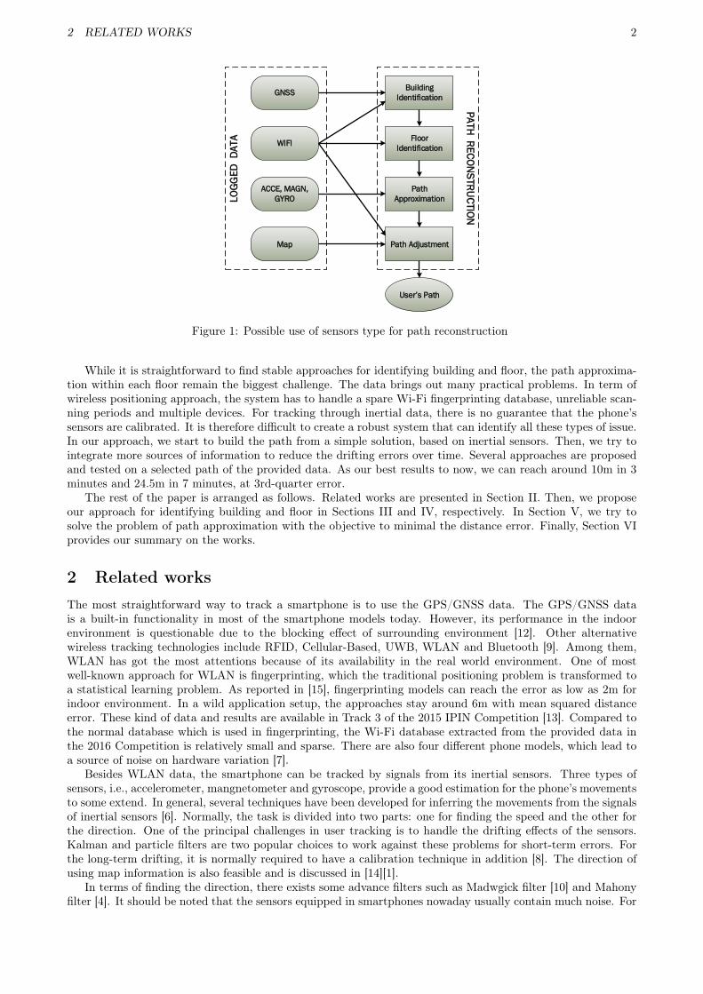
Intuitively, the process of user tracking starts from identifying building to the floor of the building and thenthe 2D positions within the floor. We select some specific subset of sensors to carry out these tasks (see Fig. 1):

• Identifying building: using GPS value (GNSS tag) and appeared Wi-Fi MAC address data (WIFI tag).

• Identifying floor: using Wi-Fi data to build fingerprinting database, then learning floor ID from thedatabase by several models.

• Approximating the 2D path: we assume that for each floor, the user needs to enter and leave at somespecific points. The remaining task is to reconstruct the path from these two locations. For solving this,we apply a particle filter. The moving model bases on the inertial data, which are accelerometer, magneticand gyroscope sensors. Additional adjustment steps are carried out, which could based on Wi-Fi data ormap information.

1

2 RELATED WORKS 2

Building

Identification

Floor

Identification

Path

Approximation

Path Adjustment

GNSS

WIFI

ACCE, MAGN,

GYRO

Map

User s Path

LO

GG

ED

D

ATA

PA

TH

RE

CO

NS

TRU

CTIO

N

Figure 1: Possible use of sensors type for path reconstruction

While it is straightforward to find stable approaches for identifying building and floor, the path approxima-tion within each floor remain the biggest challenge. The data brings out many practical problems. In term ofwireless positioning approach, the system has to handle a spare Wi-Fi fingerprinting database, unreliable scan-ning periods and multiple devices. For tracking through inertial data, there is no guarantee that the phone’ssensors are calibrated. It is therefore difficult to create a robust system that can identify all these types of issue.In our approach, we start to build the path from a simple solution, based on inertial sensors. Then, we try tointegrate more sources of information to reduce the drifting errors over time. Several approaches are proposedand tested on a selected path of the provided data. As our best results to now, we can reach around 10m in 3minutes and 24.5m in 7 minutes, at 3rd-quarter error.

The rest of the paper is arranged as follows. Related works are presented in Section II. Then, we proposeour approach for identifying building and floor in Sections III and IV, respectively. In Section V, we try tosolve the problem of path approximation with the objective to minimal the distance error. Finally, Section VIprovides our summary on the works.

2 Related works

The most straightforward way to track a smartphone is to use the GPS/GNSS data. The GPS/GNSS datais a built-in functionality in most of the smartphone models today. However, its performance in the indoorenvironment is questionable due to the blocking effect of surrounding environment [12]. Other alternativewireless tracking technologies include RFID, Cellular-Based, UWB, WLAN and Bluetooth [9]. Among them,WLAN has got the most attentions because of its availability in the real world environment. One of mostwell-known approach for WLAN is fingerprinting, which the traditional positioning problem is transformed toa statistical learning problem. As reported in [15], fingerprinting models can reach the error as low as 2m forindoor environment. In a wild application setup, the approaches stay around 6m with mean squared distanceerror. These kind of data and results are available in Track 3 of the 2015 IPIN Competition [13]. Compared tothe normal database which is used in fingerprinting, the Wi-Fi database extracted from the provided data inthe 2016 Competition is relatively small and sparse. There are also four different phone models, which lead toa source of noise on hardware variation [7].

Besides WLAN data, the smartphone can be tracked by signals from its inertial sensors. Three types ofsensors, i.e., accelerometer, mangnetometer and gyroscope, provide a good estimation for the phone’s movementsto some extend. In general, several techniques have been developed for inferring the movements from the signalsof inertial sensors [6]. Normally, the task is divided into two parts: one for finding the speed and the other forthe direction. One of the principal challenges in user tracking is to handle the drifting effects of the sensors.Kalman and particle filters are two popular choices to work against these problems for short-term errors. Forthe long-term drifting, it is normally required to have a calibration technique in addition [8]. The direction ofusing map information is also feasible and is discussed in [14][1].

In terms of finding the direction, there exists some advance filters such as Madwgick filter [10] and Mahonyfilter [4]. It should be noted that the sensors equipped in smartphones nowaday usually contain much noise. For

3 BUILDING IDENTIFICATION 3

Table 1: Number of Wi-Fi scans on UAH Building data

Route All Floor0 Floor1 Floor2 Floor3 AvgDistanceR1-S3 80 20 32 19 0 5.77R1-S4 139 23 54 45 0 4.30R2-S3 97 64 0 0 19 6.08R2-S4 149 92 0 0 36 4.82R4-S3 40 0 18 16 0 4.72R4-S4 64 0 19 38 0 4.02Total 569 199 123 118 55 4.96

Android devices, the errors can be as large as 60◦ for 3 minutes of tracking [16]. On the other hand, trackingthe user speed could be more straightforward if we can have the constraint that there are only two movementpatterns, namely standing and walking. The number of steps can be counted and then multiplied with steplength to find the moving distance [8].

3 Building Identification

In the supplementary data, each building is included with the WGS coordinates of the building. By usingthese coordinates, the distance between pair of buildings is calculated. There is only the case of UJITI andUJIUB, which have a distance of around 450m. The other pairs are quite far from each other. Beside that, eachbuilding comes with a specific set of observed MAC_BSSID. There is no MAC_BSSID belong to two buildings. Wethen assume that GNSS data and appeared MAC_BSSID could be used to identify the building efficiently.

4 Floor Identification

In this task, we select the UAH building data for validating our model because it has a high number of observedWi-Fi stations. There are 353 MAC_BSSID records appeared in the given data.

4.1 Fixing the POSI data and create the groundtruth data

The training data include POSI tag, which is the checkpoints along the user’s trajectory. The time periodbetween consecutive POSI records varies and is longer than the required sampling time, which is 0.5s. In mostcases, the user takes a linear trajectory between two subsequent POSI records. However, there are severalsegments which do not follow the observation. It is thus mandatory to correct those segments. We add somevirtual checkpoints along the ambiguous segments. The timestamp together with these virtual checkpoints arecalculated from the ratio between the virtual moving distance and the time to complete the real segment. Thosevirtual checkpoints are put manually on the basis of the provided maps and videos. The small parts where thetrajectory crosses the stairs are not corrected.

After fixing the trajectory, the position at a fixed time t will be computed by a linear interpolation betweentwo consecutive checkpoints Pi and Pj , respectively, before and after t. The Wi-Fi fingerprinting database isthen created by joining the groundtruth position with the Wi-Fi signals recorded in the log file. Each WIFI

record is provided with: application timestamp (AppTimeStamp), sensor level timestamp (SensorTimeStamp),name (Name_SSID), MAC address (MAC_BSSID) and signal strength (RSS). The SensorTimeStamp field of theWIFI record is used as the time indicator for Wi-Fi.

To produce a completed scan from WIFI records, the appeared sensor times are grouped into separated timeperiods. Each period has the length of 4.5s. Specifically, two WIFI records are considered in a same scan if thedifference in their SensorTimeStamp is less than 4.5s. From the completed scan, we create a feature vector of353 dimensions, and set the reported RSS value of seen Wi-Fi stations as the feature value. If there is an unseenWi-Fi station in the completed scan, its value is set to a constant value (WIFI_ZERO).

4.2 Wi-Fi fingerprinting results on floor identification

The UAH building comes with four floors (ID from 0 to 3). There are 3 routes in total, with two differentdevices, namely Samsung Galaxy S3 and Samsung Galaxy S4. Table 1 shows the extracted number of theWi-Fi fingerprinting data. The All column is the number of the POSI records appeared in the log file. TheAvgDistance is the average distance between consecutive completed Wi-Fi scans. The stats indicate that thetwo phone models Samsung S3 and S4 have some variation within the Wi-Fi scanning data.

5 PATH APPROXIMATING WITHIN A FLOOR 4

Table 2: Floor accuracy on 5 folds cross validation

Id Model Raw 2-filter HLF1 RF classifer 95.52% 94.28% 92.70%2 RF regressor 89.80% 91.82% 93.76%3 KNN classifier 91.47% 91.30% 91.47%4 KNN regressor 90.60% 90.33% 90.69%5 XGB classifier 98.24% 97.80% 97.36%6 XGB regressor 99.38% 98.41% 98.77%

In the task of learning the floor ID, we apply three family models: K-Nearest Neighbour (KNN), RandomForest (RF) [2] and Extreme Gradient Boost (XGB) [3]. While KNN is a popular choice to work with the Wi-Fifingerprinting data, the others propose learning abilities on a small amount of training data. We also vary theset of features:

• Raw features: The RSS value is used as default value. In case of KNN model, the Euclidean distance isused. We set WIFI_ZERO to −150.

This value is sensitive for the KNN models. The other models, based on decision tree, are unlikely affected.

• Filtering [11]: The set of features is derived from the winner of Track 3 of the 2015 IPIN Competition. Inour experiments, instead of splitting into groups like their proposal, we add an addition of D features torepresent that. The level of filters is set to two, namely 2-filters. Assume that among D access points, ifthe ith and jth ones have the highest reported RSS, we set the value of ith and jth in D additional featuresto an INFINITE value. This was can ensure the robustness of Euclide distance. The total number offeatures after this operator is 2D.

• Hyperbolic Location Fingerprinting features [7]: The feature comes from the fact that the data come fromtwo different devices. We simply take the subtraction of the RSS values as the feature between Wi-Fiaccess points i, j. Normally, using HLF features would results into D × (D − 1)/2. Because of the littleamount of data we have got, it would be unpractical for training model if we use such an large numberof dimension (around 500 samples against over 60000 dimensions). An additional dimensional reducestep thus is necessary. In our experiments, we use the Random Tree Embedding approach [5] to get a700-dimensional vector approximately.

Each type of model is tested with both options, i.e., classifier and regressor. In the floor learning task, it isstraightforward to use a classifier to learn the feature space. In case of using a regressor, the target is a realnumber indicating the floor, and the output is also a real value x in the range of [0, 3]. In order to convertingfrom x to a floor ID, we use a cut vector C = {c1, c2, c3}. A value x is classified to the Floor i if x ≤ ci+1,otherwise, x is classified as the Floor 3. The value of C could be computed directly on training data as ansub optimization step. After the regression model is trained, we get the model’s prediction values on all thetraining data. Then, C is selected in a way that maximize the prediction accuracy of the prediction values andthe training targets. On the other hand, this method yields a potential overfitting issue.

Table 2 shows the results on 5 folds random cross validation. XGB regression model with Raw feature get thehighest results. There is no significant separation between three types of features. The using of regressor withan additional layer of optimization could provide a good solution to the floor identification. It can be explainedthat the label, which is the number of floor actually, contains some continuous relationship. For example, inthe vector space, the samples of Floors 0 and 1 could be overlapped easily than those of Floors 0 and 2.

5 Path Approximating within a Floor

At this point, based on the floor cross validation results, we assume that the floor is able to be predictedcorrectly. Therefore, the remaining task is to approximate the trajectory within the floor. Moreover, as theusers can only use stairs or elevators for moving out or into the floor, the task could be reduced to find anapproximate path from a starting point. In other cases, GNSS data and Wi-Fi data could be used to find outthe point. As it is simple to produce correct groundtruth path for it, we select Floor 1 from UAH building fortesting the idea on path approximation within the floor.

5.1 Using GNSS data

The GNSS data comes with the latitude/longitude of the smartphones. Table 3 provides the details of theGNSS data within Floor 1.

5 PATH APPROXIMATING WITHIN A FLOOR 5

Table 3: GNSS data on the Floor 1 of UAH Building, the errors is reported by 3rd-quarter errors

Route N Update rate Longest missing ErrorR1-S3 44 9.5s 25.0s 466.2mR1-S4 186 2.3s 127.0s 29.4mR4-S3 14 7.7s 20.0s 15.6mR4-S4 0 - - -

Figure 2: The green dots are the training Wi-Fi points, and the blue dots denote the center of the clusters. Theradius of the clusters circle is set to 10m to visualize the quality of the clustering.

There exists a significant difference in the update rate between two phone models, Samsung Galaxy S3 andSamsung Galaxy S4. The S4 phone is updated more frequently than the S3 one. On the other hand, the S4phone suffers a large missing period. This would make using the GNSS data from the S4 less reliable. Theexpected errors for using GNSS data is around 30.0m. However, the results is likely unstable.

5.2 Inferring position using Wi-Fi data

The same feature set and models from previous experiments are used. It is straightforward that regressortype models can be applied for learning the position from the Wi-Fi data. For the classifiers, it is possible totransform the 2D coordinates target, including latitude and longitude, to a label. The most popular way is todivide the area into several smaller grids of fixed size. Another approach could involve manually picking thepoints by using the provided map. In our experiment, we perform a K-means clustering on latitude, longitudeof all the groundtruth points. Figure 2 is a result of K-mean clustering with the number of centers fixed to 15.

Table 4 reports the distance errors on 5 folds cross validation. With the total of 123 available points, theeffective training samples are around 100 points and 23 points for testing. The best result are around 6.0m byusing XGB model with 2-filters feature. In fact, there is a similar performance between three set of features.With three set of features, we prefer to use the HLF feature set because the device noise could be high, especially

Table 4: Errors on Floor 1, UAH building for 5 folds cross validation, report by 3rd-quarter errors

Id Model Raw 2-filters HLF1 RF classifer 10.6m 11.5m 12.9m2 RF regressor 13.6m 16.1m 16.4m3 KNN classifier 10.3m 10.3m 10.3m4 KNN regressor 9.7m 9.4m 9.1m5 XGB classifier 6.6m 6.0m 6.2m6 XGB regressor 9.1m 8.6m 8.7m

5 PATH APPROXIMATING WITHIN A FLOOR 6

we only have a small size of training data. With the tree-based model, classifier approaches outperform theregressor ones. At this step, we can build the user path by interpolating the outputs of the Wi-Fi model.However, like in GNSS data, there is also a long period of time that the phone does not receive any new Wi-Fidata. The errors also are unpredictable if the user moves too far from the appeared area in the training data.

5.3 Inferring direction using magnetic, accelerometer and gyroscope sensors

In order to identify the phone’s direction, we look into the data of four types of sensors: magnetic sensor (MAGNtag), accelerometers (ACCE tag), gyroscope (GYRO tag) and ahrs sensors (AHRS tag).

The sampling rate is not the same between those types of sensors and between different phone models. Inaddition to that, the rate can vary in a great range for a walk of the user For example, in the GYRO data ofS3 model, it is updated with every 5ms in average. However, at some point, it takes 25ms to get the new data.

Several ways of extracting the phone’s direction are tested, including:

• Based on magnetic and accelerometer (AccMag): at time t, the data from nearest MAGN and ACCE readare used for constructing the rotation matrix. Then, the AccMag orientation is devised from the matrix.This is the most standard way for finding the phone orientation. The value of AccMag orientation issupposed to be the low update rate part of the direction. It is then fused with the high update rate partby two other methods, which evolves the integration of the gyroscope data.

• Based on the integration of gyroscope (GYRO): the values are used to feed to the system with the SensorT imestampvalue. The integration is then calculated on 3-axis, Azimuth, Pitch and Roll. An further step of fusion isadded by using a constant α:

Gyro = (1− α)× IntegratedGyro+ α×AccMag (1)

where α is a threshold weighting contribution of these two factors.

• Use Madgwick filter [10]: the filter is designed to fix the magnetic disortion and gyroscope drifting errorsin commercial IMU. It uses a quaternion representation for accelerometer and mangnetometer data. Anoptimized gradient-descent algorithm is employed to track the gyroscope errors. In our implemenationof Madgwick filter, we downsample both gyroscope and magnetic data to be equal to the update rate ofaccelerometer data. The starting quaternion is calculated directly from the AccMag above.

• Using AHRS data directly: AHRS data is received every 0.02 second for both S3 phone and S4 phone,roughly.

From all of the approaches above, we use the value of Azimuth axis (or Yaw) as the user’s direction. Thedirection can have the update rate as high as 0.02 second, which is equal the update rate of accelerometersensor. Therefore, before intergrating with the speed, it should be downsampled.

5.4 Inferring the moving distance using accelerometer sensor

Figure 3 plots the Z-axis of accelerometer when the user’s movement contains both standing and walkingmovement. There are specific patterns in the signal. For simplicity, we calculate the standard deviation for afixed window length dt and use a threshold M for splitting between standing and moving. In order to find thesuitable value of M , the standard deviation of Z-axis is computed on all the data (Fig. 4). From the figure,there is a point which the standard deviation pattern changes significantly. In this case, the point is around0.1. Therefore, it is straightforward for choosing M = 0.1 in this case.

Whenever the standard deviation of a window length dt is above M , we infer the moving distance as:

MovingDistance = AvgSpeed× dt (2)

where AvgSpeed is the average speed over the floor, which could be calculated based on the training data. Thelocal variance of the user’s speed is discarded here. We choose to calculate the moving distance based on theAvgSpeed instead of the number of steps because the user’s step length is not available.

5.5 Combining the direction and moving distance for the full path approximating

From the calculate direction and moving distance, we downsample by a window of time length dt = 0.5 second,which meets the requirements of the competition.

The approximating path will be built by using particle filter, which is a popular choice in this task. As ourobservations on the data, it is difficult to create an effective observation model from the Wi-Fi scanning results.

5 PATH APPROXIMATING WITHIN A FLOOR 7

Figure 3: Z-axis plot of walking and standing movements

Figure 4: Cumulative density function of standard deviation for each window length of 0.2s, i.e 10 ACCE datapackages.

There are two main reasons: firstly, there exists long periods of time in the data that Wi-Fi scanning result doesnot present; secondly, after 4 seconds in general, there could be a huge drifting in the particle’s position whichcan not be adjusted by the Wi-Fi fingerprinting results. Therefore, our particle filter have only the movingmodel.

To evaluate our approaches, we choose the Route 1 at UAH building. The data is extract from the user’swalk with the Samsung Galaxy S3 phone model. The period when the phone entered and left the Floor 1 isfrom 132.25s to 565.00s, approximately. To prevent the drifting errors, we use only 3 minutes from that periodlength.

Table 5 shows the results in term of mean squared distance error (MSE), mean error and 3rd quarter error.During a period of 3 minutes, Gyro and Madgwick Filter reach a similar error of 20.0m. The Gyro approachstill is more stable than the Madgwick filter as it has both a low MSE and the median error. Meanwhile, theothers, AccMag and AHRS, cannot provide a good approximation of the phone’s direction.

We plot the output paths in Fig. 5. The turning angles from the Gyro and Madgwick filter are highlycorrelated with the user’s movements. The under-performance of Madqwick filter could come from our specificimplementation on the identifying the first quaternion. The technique suggests that a motion stop is needed,instead of calculating it directly as in ours. In addition to that, there is a downsampling step for GYRO and MAGN

data, which could introduce more noise.Compare to the performance of Gyro and Madwick filter, the correlation of AHRS and AccMag is quite low.

It is reported that the magnetic sensor has a poor performance in the indoor environment. Moreover, thereis not guarantee that a calibration process of the magnetic sensor is carried before the data is collected. Asthe magnetic data are presented in computing the direction of Gyro and Madgwick filter approaches, it couldpossibly reduce the accuracy of those output directions.

5.6 Path adjusting

In the above setup, the drifting error could be as high as 20m after only 3 minutes approximation. For a longerperiod, i.e. 7 minutes in this specific case, the error is likely unpredictable. Therefore, additional calibrationsteps should be employed for controlling the drifting affects. There are several sources of data could be usedfor this purpose, which includes GNSS, Wi-Fi and map information. Comparing between GNSS and Wi-Fi, theWi-Fi data has a more stable update rate and also a better accuracy. Therefore, using the Wi-Fi data to adjust

5 PATH APPROXIMATING WITHIN A FLOOR 8

Table 5: MSE distant errors, median and 3rd-quarter errors for in 3 minutes

Technique MSE Median 3rd-quarterAccMag 43.7m 11.7m 65.0mGyro 13.12m 6.5m 19.4m

Madgwick Filter 17.2m 12.4m 20.4mAHRS 39.0m 17.1m 55.5m

(a) AccMag direction (b) Gyro direction (c) Use Madgwick filter(d) Use AHRS data pack-age

Figure 5: The generate paths from the 4 techniques. The blue line is the real trajectory, the green path is thegenerated ones.

the position is quite a popular approach, including [8] or the on-site Track 1 of the 2015 IPIN Competition [13].On the other hand, integrating the map information for calibrating the errors could possibly make the systemless stable. Moreover, the performance highly depends on the environment and on how map is modeled. Forexample, [1] uses the assumption that the building has a rectangle shape for reducing the direction drifting. In[14], the map information is used at different levels, including using polygons to model the floor. In this section,we are going to explore several directions of using Wi-Fi and map information to get stable results.

5.6.1 Combine Wi-Fi data and the path approximation

It is unlikely that the observation model built on the Wi-Fi fingerprinting results can calibrate the driftingerrors generated by the sensors of the smartphone. However, whenever the phone complete a Wi-Fi scan, wecan have a small adjustment of the particles at that specific time t. Let the Wi-Fi feature vector at time t is X,and Y is the position estimated by the Wi-Fi fingerprinting model. A particle P then can be pulled to positionPnew near M with a constant λ:

Pnew = P + λ× (Y − P ) (3)

In the next section, we extend the above idea by identifying a local value of Y base on the results of classifiermodel. From the results of Wi-Fi fingerprinting in a cross validation scheme, it can be concluded that theclassifier outperforms the regression. In order to employ the classifier output efficiently, we use the predictionprobability of each class. Given there are N classes, the output of each model (KNN, RF or XGB) for a sampleX can be in the form of:

probX = {p1, p2, ..., pN} (4)

where pi is the probability of X belonging to centers Ci. At the time of adjusting position for a particle P ,we already know the its position. It is thus possible to find the three most nearest centers around P . Forexamples, let them be C1, C2 and C3. The corresponding probability are p1, p2 and p3. Those probability thenis normalized to have the sum being equal to 1. The estimated position Y is the weighted sum of the threecenters C1, C2 and C3 with the p1, p2 and p3 are the coefficients:

Y = p1 × C1 + p2 × C2 + p3 × C3 (5)

5.6.2 Adjust the wall-crossing step

This is the most straightforward usage of map information. The movement of each particle is constraint bywalls. Those wall is drawn manually from the provided map data. If a particle goes cross a wall, its directionis adjust to go parallel with the wall.

5 PATH APPROXIMATING WITHIN A FLOOR 9

Figure 6: Apply local adjustments for fixing wall crossing. The wall is colored with the cyan

Figure 6 illustrates this idea. For simplicity, some of the door along the walls are ignored. By applying theadjustment on the Gyro approach from above, we can have the 3-quarter error distance stays around 11.2m,which is a significant reduction from 19.4m. This approach could be efficient for stabilizing the errors in a shortterm. On the other hand, its performance depends on the properties of the area where the user is standing.When the user goes to the large hall, where there is no wall, the accuracy is heavily affected by the drifting indirection.

In the capability to fix long-term drifting, this approach is still not sufficient. The adjustment operatorsonly have local effects. As we can see from Fig. 6, the source of the errors is not at the time when the particlecrosses the walls. It come from a changing direction at some place in the previous path. Thus, it leads us to amore complicated approach.

5.6.3 Minimize the number of wall crossing

In this part, we try to define an optimization problem for path adjusting. Firstly, we create two necessaryoperators for changing the path. Assuming that the errors mainly come from the noisy magnetic data in indoorenvironment, a rotation operator could be apply to fix. Moreover, the using of AvgSpeed is not flexible enoughto describe the velocity of the user. In general, the user can move faster or slower than the AvgSpeed. Therefore,an additional normalization operator is needed for deriving the local speed from the global AvgSpeed.

At this step, it is sufficient to find an optimal set from these two operators with the objective is to minimizethe number of wall-crossing. However, to reduce the search space and also make the results more illustrative,we divide the map of each floor into smaller regions. Each region will have several pivot points and its walls.The pivot points are used to signal the entering or leaving the regions. We then define the cost of a path withina region as the number of wall-crossing by following the path.

Beside that, the user’s movement pattern can be split into two types, i.e., move straight and turn, on thebasis of the output direction. For example, Fig. 7 plots the standard deviation on the direction for each timewindow of 2.5s.

A simple threshold of 0.25 is enough for classifying each small window length. Once each small part isassigned with a label, we use those parts as the seeds and extend their two endpoints. The extension process isterminated when a part with a different label is reached. The sequence is divided into a list of sub-parts. Twoconsecutive sub-parts are two different kinds of movement. We then put more constraints on the operators.The rotation operator can be used only on the turn sub-part, and the normalize operator can be used only onthe move straight sub-part. Moreover, we only allow the starting of a new region after a turn sub-part.

To find a proper solution for the optimization problem, we employ a greedy strategy. From the startingconfiguration, the first collision with walls will be detected. Then the nearest previous turn and move straightsub-parts are selected to apply the two operators. The searching range of each operator is chosen from apredefined range. The range should reflect the standard deviation errors in the process of inferring movementspeed and direction.

5 PATH APPROXIMATING WITHIN A FLOOR 10

Figure 7: Standard deviation of the inferred angle for each window time 2.5s

Figure 8: The new path after optimizing the numbers of wall crossing.

Figure 8 presents the results of the optimization process. The map are derived from the wall-crossing stepby adding several points for the pivot locations. The regions are split on the basis of its wall characteristicswith the purpose is to reduce the complexity of the searching step. Additional pivot points are added at thestairs and elevators.

In our setup, the range of rotate is set within 10◦and the range of normalization operator is set to have amaximum absolute value of 0.1m/s. The output approximation path has a 3rd-quarter error distance of 11.2m.Like the wall-crossing adjustment, this approach depends heavily on the map configuration. For example, therole of long horizontal corridor is sensitive to the error reduction process. By applying a fix operator here, theremaining path is rotated toward the real path. On the other hand, in the large hall, where there are only afew walls, it becomes difficult to find the suitable adjustment because there is no error.

A global minimum could be reached by using a dynamic programming approach. However, it is difficult toensure that the global solution is better than the local one, in term of distance error. Moreover, it would requirea more complicated model to represent all the constraints in the problem. For example, the objective functionshould include a cost between choosing a normalization operators instead of a rotate operators. On the otherhand, a more complex map model could lead to overfitting.

5.7 Combining several adjustment strategies

The adjustment steps above are combined in several ways to produce the outputs, which is listed in Table 6.More specifically, the Wi-Fi output only adjust the particles by the output position of Wi-Fi fingerprinting

6 CONCLUSION 11

Table 6: Distance errors at 3rd-quarter for 3 minutes and 7 minutes walking

Technique 3 minutes 7 minutesWi-Fi 16.4m 29.8mWall + Wi-Fi 14.2m 28.1mOptimizing + Wall + Wi-Fi 10.1m 24.5m

model. In case of Wall + Wi-Fi, the particles are adjust to avoid hitting the wall first, then use the positions ofWi-Fi as above. The third approach runs the optimize algorithm on the generated directions, then is continuedto process as in the second system. In all three approaces, the Gyro direction is preferred to used

The results in Table 6 are reported by running approximation for 3 minutes and 7 minutes, which are a halfand full path of the floor, respectively. The best performance is the third system with around 25.0m errors at3rd-quarter. The high errors of it could be explained by the three walking on long corridors in the Route 1, atFloor 1 of UAH building. If the system miss any of these paths, its distance error will increase greatly.

In term of avoiding overfitting, the Gyro + Wall system seems to be the most robust one. The two otherones’ performance could depend on the characteristics of the path and the user’s walking route to some extent.It is needed a more complete evaluation to choose the best approach. However, we are unable to make itavailable at this point because of the time constraint.

6 Conclusion

The data provided at IPIN 2016 Competition is very closed to the real world data. It thus comes with manypractical problems. In this paper, we introduce the works for solving the tracking problems. There are someparts of the problems, e.g., building identification and floor identification, can be solved in a straightforwardmanner. On the other hand, when it comes to the path approximation, the system error becomes unpredictable.Through our understanding of the problems to point, a distance error of 30.0m at 75th percentile can be reachedeasily. However, it is quite difficult to match the performance which is described in the literature. For stabilizingour results, we try to find some alternative ways to reduce the long-term drifting. These proposed methods aretested and have good results on the selected data, though, they are at the very beginning of the work. Thereare many rooms left to make our approaches improve on a larger scale.

References

[1] Khairi Abdulrahim, Chris Hide, Terry Moore, and Chris Hill. Using constraints for shoe mounted indoorpedestrian navigation. Journal of Navigation, 65(01):15–28, 2012.

[2] Leo Breiman. Random forests. Machine learning, 45(1):5–32, 2001.

[3] Tianqi Chen and Carlos Guestrin. Xgboost: A scalable tree boosting system. CoRR, abs/1603.02754, 2016.

[4] Mark Euston, Paul Coote, Robert Mahony, Jonghyuk Kim, and Tarek Hamel. A complementary filter forattitude estimation of a fixed-wing uav. In 2008 IEEE/RSJ International Conference on Intelligent Robotsand Systems, pages 340–345. IEEE, 2008.

[5] Pierre Geurts, Damien Ernst, and Louis Wehenkel. Extremely randomized trees. Machine learning, 63(1):3–42, 2006.

[6] Robert Harle. A survey of indoor inertial positioning systems for pedestrians. IEEE CommunicationsSurveys & Tutorials, 15(3):1281–1293, 2013.

[7] M.B. Kjaergaard and C.V. Munk. Hyperbolic location fingerprinting: A calibration-free solution for han-dling differences in signal strength (concise contribution). In Pervasive Computing and Communications,2008. PerCom 2008. Sixth Annual IEEE International Conference on, pages 110–116, March 2008.

[8] Nisarg Kothari, Balajee Kannan, Evan D Glasgwow, and M Bernardine Dias. Robust indoor localizationon a commercial smart phone. Procedia Computer Science, 10:1114–1120, 2012.

[9] Hui Liu, Houshang Darabi, Pat Banerjee, and Jing Liu. Survey of wireless indoor positioning techniquesand systems. IEEE Transactions on Systems, Man, and Cybernetics, Part C (Applications and Reviews),37(6):1067–1080, 2007.

REFERENCES 12

[10] Sebastian Madgwick. An efficient orientation filter for inertial and inertial/magnetic sensor arrays. Reportx-io and University of Bristol (UK), 2010.

[11] A. Moreira, M. J. Nicolau, F. Meneses, and A. Costa. Wi-fi fingerprinting in the real world - rtls@um atthe evaal competition. In Indoor Positioning and Indoor Navigation (IPIN), 2015 International Conferenceon, pages 1–10, Oct 2015.

[12] Veljo Otsason, Alex Varshavsky, Anthony LaMarca, and Eyal De Lara. Accurate gsm indoor localization.In International conference on ubiquitous computing, pages 141–158. Springer, 2005.

[13] Francesco Potortì, Paolo Barsocchi, Michele Girolami, Joaquín Torres-Sospedra, and Raúl Montoliu. Evalu-ating indoor localization solutions in large environments through competitive benchmarking: The evaal-etricompetition. In Indoor Positioning and Indoor Navigation (IPIN), 2015 International Conference on, pages1–10. IEEE, 2015.

[14] O. Woodman. Pedestrian Localisation for Indoor Environments. PhD dissertation, University of Cambridge,2010.

[15] Moustafa A Youssef, Ashok Agrawala, and A Udaya Shankar. Wlan location determination via cluster-ing and probability distributions. In Pervasive Computing and Communications, 2003.(PerCom 2003).Proceedings of the First IEEE International Conference on, pages 143–150. IEEE, 2003.

[16] Pengfei Zhou, Mo Li, and Guobin Shen. Use it free: instantly knowing your phone attitude. In Proceedingsof the 20th annual international conference on Mobile computing and networking, pages 605–616. ACM,2014.