SMART MODELING OF OPTIMAL INTEGRATION OF HIGH ......CCGT Combined Cycle Gas Turbine CCS Carbon...

FINAL REPORT

Thomas Ackermann

Stanislav Cherevatskiy

Tom Brown

Robert Eriksson

Afshin Samadi

Mehrdad Ghandhari

Lennart Söder

Dietmar Lindenberger

Cosima Jägemann

Simeon Hagspiel

Vladimir Ćuk

Paulo F. Ribeiro

Sjef Cobben

Henrik Bindner

Fridrik Rafn Isleifsson

Lucian Mihet-Popa

Supported by: Project Partners:

Energynautics GmbH, Germany

University of Cologne, Germany

KTH Royal Institute of Technology, Sweden

DTU Technical University of Denmark

TUE Eindhoven University of Technology, Netherlands

SMART MODELING OF OPTIMAL INTEGRATION OF HIGH PENETRATION OF PV – SMOOTH PV

13. May 2013 (Version 1.0)

Copyright Information

All content of this report is Copyright © Energynautics, UoC, KTH, DTU and TUE 2013.

Unless otherwise stated, the content (including text, graphics, logos, images and

attached documents), design and layout of this report is the property of Energynautics,

UoC, KTH, DTU and TUE. Any unauthorized publication, copying, hiring, lending or

reproduction is strictly prohibited and constitutes a breach of copyright.

EXECUTIVE SUMMARY

http://www.smooth-pv.info 3

EXECUTIVE SUMMARY

In the Smooth PV project several partners with diversified backgrounds united to

analyze the implications associated with high penetration of photovoltaics in the

electrical power system and to develop models (mostly in DIgSILENT PowerFactory) for

conducting simulation studies. The focus is laid upon both the European transmission

network and the distribution grid, since a high PV share affects the system both at the

global and the local levels.

On the European transmission system level Energynautics and UoC studied scenarios

for the future possible development of the generation and grid infrastructures assuming

large increases in renewable energy generation, PV in particular. This was done using

UoC’s Electricity Market Model and Energynautics’ Transmission System Model.

The Electricity Market Model is a long-term investment and dispatch model for

renewable and conventional energy, as well as storage and transmission technologies

covering 29 countries (EU27 plus Norway and Switzerland). With the help of this model

it was simulated how installed capacities and their operation will develop in the future

given a set of assumptions regarding techno-economic conditions as well as the

regulatory framework. Among other inputs, special attention was given to the

determination of the capacity credit of PV, measuring the contribution of PV to the

system’s security of supply. It was found that from a conservative point of view, the

capacity credit of PV should be assumed to be 0% for all EU member states, due to an

electricity demand structure that is characterized by high levels during evening hours

when no PV generation is available.

Energynautics’ European Transmission System Model was updated and made suitable

for AC load flow calculations, so that reactive power flow, losses and AC-related stability

issues could be accounted for. The model was furthermore validated by comparing the

calculated cross-border flows between European countries with the publicly available

data and optimizing so that good agreement was achieved. As the future power system

is expected to contain a number of High Voltage Direct Current (HVDC) lines for long-

distance transmission of renewable energy, a methodology for the optimal placement,

sizing and operation of these lines was developed. These lines are integrated into the AC

meshed network in such a way that the loading of the AC system is reduced to the

maximum possible degree and loop flows are avoided.

In order to be able to include transmission grid extensions in the long-term market

simulation, a methodology was developed that allows optimizing power generation and

transmission infrastructures jointly through an iterative approach based on power

transfer distribution factors (PTDFs). The algorithm proved to be applicable and

convergent for both small scale and large scale models. The methodology was applied in

a detailed study of the European power sector aiming at ambitious CO2 emission

reductions in order to analyze the system value of optimized grid extensions within this

http://www.smooth-pv.info/

EXECUTIVE SUMMARY


context. While accumulated discounted total system costs until 2050 amount to 2833

bn. € in the case of a joint optimization of generation, storage and grid capacities

(optimal grid extension), they amount to over 3424 bn. € if the grid is only marginally

extended until 2050 (minimal grid extension). The significant cost difference of 591 bn. €

(20.9%) clearly demonstrates that significant grid extensions help to cost-efficiently

deploy renewable power sources in Europe. The share of PV in the yearly load coverage

in 2050 reaches 32 % when the grid is extended in an optimal manner, and 23 % when

the grid is only marginally extended. It was also demonstrated that these future

scenarios for the power system are able to withstand extreme weather events, such as a

prolonged period of 10 days with low wind and little sun, with no hazard to the security

of supply.

In order to estimate the maximum feasible penetration of photovoltaics in the

European power system in terms of the energy used from PV systems, Energynautics

calculated several scenarios with various assumptions concerning available storage

capacities distributed throughout Europe. It was shown that a share for PV of around 30-

40 % of total yearly consumption can be feasibly accommodated in the system without

any major transmission line upgrades, while making sure that the amount of required

storage is realistic and the amount of curtailed PV energy is kept to a minimum. This

maximum feasible penetration chimes well with the cost-optimal results calculated in

the iterations with the Electricity Market Model, where calculations in the scenario with

optimal grid extensions yielded PV’s share of 32 %.

UoC applied the long-term market simulation model to analyze the effect of PV grid

parity in Germany. Under the current regulatory framework, investments in residential

PV systems (in combination with small-scale storage units) are triggered as the gap

between the levelized costs of electricity (LCOE) of PV and the retail electricity tariff

grows, mainly due to the fact that self-consumed electricity is exempted from paying

network tariffs, taxes, levies and other surcharges. However, while the consumption of

self-produced PV electricity on the household level induced by the exemption from

these extra charges might be beneficial from the perspective of single households, it is

inefficient from the total system perspective. In this part of the study, the consequences

of PV grid parity in Germany until 2030 have been analyzed from both the single

household and the total system perspective. In the former case, the optimal PV and

storage system capacities are found to increase with the number of residents in the

household, enabling them to cover on average 72 % of their annual electricity demand

by self-produced PV electricity. Furthermore, the inefficiency caused by the partial

optimization of single households (induced by PV grid parity) leads to significant excess

costs of 7.1 bn. €2011 in 2030 compared to the cost-optimal solution achieved under a

total system optimization.

For analyzing the interactions with the distribution grid, KTH and DTU developed PV

models that include maximum power point tracking and different voltage control

schemes, in addition to wind speed and ambient temperature dependencies. These


EXECUTIVE SUMMARY


models were validated and used for analysis of the effectiveness for voltage regulation

on the distribution feeders by means of reactive power (KTH) and active power (DTU).

Voltage regulation using reactive power was considered using two droop-based

methods. The first method, active power dependent voltage control, uses the local

active power production to give the reactive power set-point. This method has the

advantage of simplicity, but it does not target the voltage directly. The second method,

droop-based voltage control, gives the reactive power set-point based on the local

voltage measurement. This has the advantage that it addresses the voltage directly, but

care must be taken to coordinate nearby systems to avoid negative interactions. Both

methods show better performance, such as lower reactive power consumption and a

better voltage profile, than the standard German LV Grid Code. The voltage control

interactions are evaluated in addition to the controllability of reactive or active power

change in a node. The R/X ratio has a large impact and a higher ratio reduces the impact

of reactive power control of the voltage.

With the developed models of an electrical storage system and an office building,

voltage control based on active power was studied using two methods. The first method

is voltage control by load shifting, where the model of an office building is used to

develop a controller that regulates the electric power consumption of space heaters in

the building to shift the consumption in accordance with the system voltage. This

enables reduction of voltage spikes when PV production is high and consumption might

otherwise be low. The second method for voltage control uses energy storage to store

the energy produced by the PV plants when the production exceeds the consumption to

such a degree that overvoltage problems occur. The chosen method of voltage control

depends on the availability of manageable consumption in the local area of the PV plant.

For areas with higher consumption during the PV plant production time, the first choice

would be to utilize this available resource to provide grid support. If the local area has

low consumption the alternative would be to have some storage units installed to

support the grid during the peak production hours.

TUE concentrated on the power quality of the distribution networks with a high share of

PV inverters. To this end, a harmonic model was developed for harmonic analysis based

on laboratory measurements. The model includes both the emission of inverters and the

influence of their output impedance on the resonances in the system. A case study of a

LV network with a large number of inverters was analyzed for this purpose. It was

shown how the capacitance of inverters can influence the network resonances, and the

effect of different modeling assumptions on the calculated system impedance. The

aggregation of harmonic currents of multiple inverters was analyzed based on a field

measurement, and a modification of the existing summation coefficients was proposed

for the case of PV inverters. The existing recommendation leads to underestimation of

the aggregated harmonic current in the case of PV inverters, and it should be updated

based on measured data.


EXECUTIVE SUMMARY


Fault-Ride-Through capability and voltage support provided by inverters during short-

circuits in the distribution network were analyzed based on dynamic computer

simulations. It was found that inverters offer very limited voltage support if their current

is limited to a value close to the nominal. This question should be investigated further in

terms of the fault ride through requirements for inverters, which could prevent a

significant increase in the number and depth of voltage dips in a scenario where a large

number of synchronous generators are substituted by inverter-interfaced generators.


THE CONSORTIUM


THE CONSORTIUM

Energynautics GmbH, Germany

Project Manager: Thomas Ackermann

[email protected]

University of Cologne, Chair of Energy

Economics, Cologne, Germany

Contact: Dietmar Lindenberger

[email protected]

Royal Institute of Technology (KTH)

Electric Power Systems, Stockholm, Sweden

Contact: Prof. Lennart Söder

[email protected]

Robert Eriksson

[email protected]

Risø National Laboratory for Sustainable Energy

(DTU), Technical University of Denmark,

Copenhagen, Denmark

Contact: Henrik Binder

[email protected]

Eindhoven University of Technology (TUE),

Electrical Power Systems, Eindhoven, The

Netherlands

Contact: Prof. Will Kling

[email protected]


ABBREVIATED TERMS


ABBREVIATED TERMS

AA-CAES Advanced Adiabatic Compressed Air Energy Storage

AC Alternating Current

APD Active Power Dependent

CAES Compressed Air Energy Storage

CCGT Combined Cycle Gas Turbine

CCS Carbon Capture and Storage

CHP Combined Heat and Power

CIS Commonwealth of Independent States

CN Conditional Number

CSP Concentrating Solar Power

DAQ Data Acquisition

DBV Droop Based Voltage

DER Distributed Energy Resources

DC Direct Current

DFT Discrete Fourier Transformation

DSL DIgSILENT Simulation Language

DSM Demand Side Management

DSO Distribution System Operator

ENTSO-E European Network of Transmission System Operators for Electricity

EU European Union

FOM Fixed Operation and Maintenance

FRT Fault-Ride-Through

GUI Graphical User Interface

HV High Voltage

HVAC High Voltage Alternate Current

HVDC High Voltage Direct Current

LCOE Levelized Costs of Electricity

LV Low Voltage

MENA Middle East and North Africa

MIMO Multiple-Input Multiple-Output

MPPT Maximum Power Point Tracking

MV Medium Voltage

NREAP National Renewable Energy Action Plans

OCGT Open Cycle Gas Turbine

OLTC On-load Tap Changer

OPF Optimal Power Flow

PCC Point of Common Coupling

PFC Power Factor Correction

PoC Point of Connection

POD Power Oscillations Damping

PTDF Power Transfer Distribution Factor

PV Photovoltaic


ABBREVIATED TERMS


PWM Pulse Width Modulation

RES Renewable Energy Sources

RES-E Renewable Energy Sources for Electricity

RGA Relative Gain Array

ROCOF Rate of Change of Frequency

SOC State of Charge

SVD Singular Value Decomposition

TDD Total Demand Distortion

THD Total Harmonic Distortion

TYNDP Ten-Year Network Development Plan

VRB Vanadium Redox Battery

VSC Voltage Source Converter


CONTENTS


CONTENTS

EXECUTIVE SUMMARY ................................................................................................. 3

THE CONSORTIUM ....................................................................................................... 7

ABBREVIATED TERMS ................................................................................................... 8

1. INTRODUCTION AND ACKNOWLEDGEMENT .......................................................... 14

2. MOTIVATION FOR THIS PROJECT / BRIEF OVERVIEW OF CURRENT STATUS OF PV IN

EUROPE ................................................................................................................. 21

2.1 Motivation for this project .................................................................................. 21

2.2 Brief Overview of Current Status of PV in Europe .............................................. 22

2.3 Key Technical Features of Photovoltaic Systems ................................................ 24

3. KEY ISSUES OF PV INTEGRATION INTO POWER SYSTEMS ....................................... 26

3.1 Power Variations from PV ................................................................................... 26

3.1.1 Smoothing Effects ................................................................................... 26

3.1.2 Ramp Rates ............................................................................................. 27

3.1.3 Forecasting Issues ................................................................................... 27

3.2 Role of the Electricity Grid, Storage and DSM .................................................... 29

3.3 Issues in the Distribution Network ...................................................................... 32

3.3.1 Voltage Variations in Distribution Networks due to PV ......................... 32

3.3.2 Voltage Control Issues / Coordination of PV .......................................... 32

3.3.3 Power Quality Issues ............................................................................... 34

3.4 Issues in the Transmission Network .................................................................... 36

3.4.1 Power System Ancillary Services ............................................................ 36

3.4.2 Reactive Power Support ......................................................................... 36

3.4.3 Voltage Control Issues ............................................................................ 36

3.4.4 Inertia Issues Related to High Share of PV .............................................. 37

3.4.5 Grid Code Issues / 50.2 Hz Issue ............................................................. 37

3.4.6 Operation Rules / Setpoints .................................................................... 39

3.5 System Planning .................................................................................................. 40

3.5.1 Electricity Market Modeling ................................................................... 41


CONTENTS


3.6 Market Issues ...................................................................................................... 42

3.6.1 Capacity Credit ........................................................................................ 42

3.6.2 PV Grid Parity .......................................................................................... 42

4. APPLIED METHODS ................................................................................................ 44

4.1 Role of Modeling ................................................................................................. 44

4.2 European Transmission Network Model ............................................................ 45

4.2.1 Updating of European Model and Transition from a DC to an AC Load

Flow ......................................................................................................... 45

4.2.2 Placing and Sizing of HVDC Lines inside AC Networks ............................ 47

4.2.3 Operation of HVDC Lines in AC Networks .............................................. 49

4.2.4 Validation of the Transmission Network Model ..................................... 49

4.3 Electricity Market Model ..................................................................................... 50

4.3.1 Model Core ............................................................................................. 51

4.3.2 Scenario Assumptions ............................................................................. 54

4.3.3 Typical Days ............................................................................................ 56

4.4 Coupling of Market and Network Models........................................................... 59

4.4.1 Market Model Specifications for the Model Coupling ........................... 60

4.4.2 Network Model Specifications for the Model Coupling ......................... 61

4.4.3 Robustness Test 1: Extreme Events ........................................................ 62

4.4.4 Robustness Test 2: AC Checks................................................................. 63

4.5 Models of PV, Storage and an Office Building for Distribution System .............. 64

4.5.1 PV Models for the Distribution System .................................................. 64

4.5.2 Model of a Storage Unit for the Distribution System ............................. 68

4.5.3 Model of an Office Building .................................................................... 70

4.5.4 Model of the Distribution Grid ............................................................... 70

4.6 Method Used for Harmonic Distortion Modeling ............................................... 70

4.7 Method Used for Voltage Dip Studies................................................................. 72

5. KEY RESULTS ......................................................................................................... 74

5.1 Power Variations from PV ................................................................................... 74

5.1.1 Smoothing Effects ................................................................................... 74

5.1.2 Ramp Rates ............................................................................................. 77


CONTENTS


5.2 Role of the Electricity Grid, Storage and DSM .................................................... 78

5.2.1 CAES Potentials ....................................................................................... 78

5.2.2 Impact of the Electricity Grid and Storage on PV Utilization .................. 80

5.3 Issues in the Distribution Networks .................................................................... 84

5.3.1 Voltage Variations in Distribution Networks due to PV ......................... 84

5.3.2 Voltage Control Issues / Coordination of PV .......................................... 84

5.3.3 Power Quality Issues ............................................................................... 92

5.3.4 Voltage Dip Studies ............................................................................... 101

5.4 System Planning ................................................................................................ 105

5.4.1 Cost-optimal Power System Extension Under Flow-based Market

Coupling and High Shares of Photovoltaics .......................................... 105

5.4.2 Results of Extreme Event Tests ............................................................. 118

5.4.3 Results of AC checks ............................................................................. 121

5.5 Market Issues .................................................................................................... 122

5.5.1 Capacity Credit ...................................................................................... 122

5.5.2 The Economic Inefficiency of Grid Parity: The Case of German

Photovoltaics in Scenarios until 2030 ................................................... 128

6. CONCLUSIONS AND FUTURE WORK ..................................................................... 133

6.1 Conclusions ....................................................................................................... 133

6.1.1 Issues in the Transmission Network ..................................................... 133

6.1.2 Issues in the Distribution Network ....................................................... 134

6.2 Future Work ...................................................................................................... 136

6.2.1 Coupling of the Transmission Grid Model and the Economic Market

Model for System Planning Studies ...................................................... 136

6.2.2 Voltage Control in the Distribution Grids ............................................. 137

6.2.3 Power Quality in Distribution Networks ............................................... 137

6.2.4 Inertia Issues Related to High Share of PV ............................................ 137

6.2.5 Grid Code Issues / 50.2 Hz Issue ........................................................... 138

6.2.6 Operational Issues ................................................................................ 138

7. BIBLIOGRAPHY .................................................................................................... 140

8. APPENDIX ........................................................................................................... 146


1 INTRODUCTION &

ACKNOWLEDGEMENT

INTRODUCTION


1. INTRODUCTION AND ACKNOWLEDGEMENT

Energynautics

Milestone 2 – Update EU Model

The update to the Energynautics’ European Transmission Network Model is described in

chapter 4.2, particularly in section 4.2.1 concerning the transition from DC to AC, and in

sections 4.2.2 and 4.2.3 concerning placing, sizing and operating HVDC lines in AC

networks. This is also described in the following publication from the appendix:

T. Brown, S. Cherevatskiy, E. Tröster “Transporting the Renewables: Systematic

Planning for Long-Distance HVDC Lines”, EWEA Conference Proceedings, Vienna,

Austria 2013

Milestone 3 – Validate EU Model

Section 4.2.4 describes the validation method and the achieved results.

Milestone 4 – Simulate Impact on EU Model

Section 4.4 provides a detailed description of how the Transmission Network Model and

UoC’s Electricity Market Model were coupled for the simulation of the impact of high

penetration of PV. The simulation results are described in detail in section 5.4.

A further analysis of a large amount of PV on PV utilization is studied in section 5.2.2.

The following two publications covering these topics can be found in the appendix:

S. Hagspiel, C. Jägemann, D. Lindenberger, S. Cherevatskiy, E. Tröster, T. Brown

„Cost-optimal Power System Extension Under Flow-based Market Coupling and

High Shares of Photovoltaics“, published in Proceedings to the 2nd International

Workshop on Integration of Solar Power into Power Systems, November 2012,

Lisbon, Portugal

S. Cherevatskiy, E. Tröster “Determining the Maximum Feasible Amount of

Photovoltaics in the European Transmission Grid with Optimal PV Utilization”,

published in Proceedings to the 2nd International Workshop on Integration of Solar

Power into Power Systems, November 2012, Lisbon, Portugal

Acknowledgement

This research was funded with grant number 0325272 by the German Federal Ministry

for the Environment, Nature Conservation and Nuclear Safety. Responsibility for the

contents of this publication lies with the authors.


INTRODUCTION


University of Cologne (UoC)

Milestone 6 – Develop Economic Model

Section 4.3 provides a detailed model description.

Sections 5.4 and 5.5.2 present two applications of the model, based on two publications

(attached in the appendix):

C. Jägemann, S. Hagspiel, D. Lindenberger “The economic inefficiency of grid parity:

The case of German photovoltaics in scnearios until 2030”, published in

Proceedings to the 2nd International Workshop on Integration of Solar Power into

Power Systems, November 2012, Lisbon, Portugal





Lisbon, Portugal

Milestone 7 – Capacity Credit of PV and Storage Options

In Section 5.5.1 the capacity credit of PV is analyzed.

Section 5.2.1 summarizes the results of a systematic review of relevant literature on the

potential of CEAS in Europe.

Milestone 8 – Support Energynautics

Section 4.4 describes the cooperation between UoC and Energynautics, which is based

on an iteration of the Market Model (UoC) and the European Transmission Network

Model (Energynautics).

Section 5.4 presents the results of the cooperation, based on the publication





Lisbon, Portugal

Milestone 9 – Final Report

Acknowledgement

This research was funded through the Smart Modeling of Optimal Integration of High

Penetration of PV (Smooth PV) project with grant number 0325272 by the federal state

of North-Rhine Westphalia. Responsibility for the contents of this publication lies with

the authors.


INTRODUCTION


Royal Institute of Technology (KTH)

Milestone 14 – PV Models for Voltage Control

Can be found in Section 4.5.1.

Publications:

D. Jose, "Comparison of a three phase single stage PV system in PSCAD and

PowerFactory", 2012. EES Examensarbete / Master Thesis, XR-EE-ES 2012:013

http://www.diva-portal.org/smash/record.jsf?searchId=3&pid=diva2:558839

F. Mahmood, "Improving the Photovoltaic Modelin PowerFactory", 2012. EES

Examensarbete / Master Thesis, XR-EE-ES 2012:017


Milestone 15 – Validation of PV Simulation Models

Can be found in Section 4.5.1.

Publications:

D. Jose, "Comparison of a three phase single stage PV system in PSCAD and

PowerFactory", 2012. EES Examensarbete / Master Thesis, XR-EE-ES 2012:013


Samadi, R. Eriksson, D. Jose, F. Mahmood, M. Ghandhari, L. Söder "Comparison of a

Three-Phase Single-Stage PV System in PSCAD and PowerFactory”, published in

Proceedings to the 2nd International Workshop on Integration of Solar Power into

Power Systems, November 2012, Lisbon, Portugal

Milestone 16 – Simulate Control and Dimensioning Issues

Can be found in Section 3.3.1, 3.3.2, 3.4.3, 5.3.1 and 5.3.2.

Publications:

A. Samadi, R. Eriksson, L. Söder “Evaluation of Reactive Power Support Interactions

Among PV Systems Using Sensitivity Analysis", published in Proceedings to the 2nd

International Workshop on Integration of Solar Power into Power Systems,

November 2012, Lisbon, Portugal

A. Samadi and R. Eriksson, “Equivalent modeling of several PV power plants”,

Internal report, 2013, KTH, Stockholm

A. Samadi, R. Eriksson and L. Söder "Coordinated droop based reactive power

control for distribution grid voltage regulation with PV systems", Internal report,

2013, KTH, Stockholm





INTRODUCTION


Acknowledgement

We would like to acknowledge Swedish Energy Agency for financial support of the KTH-

part of the project.

Technical University of Denmark (DTU)

Milestone 10 – Model Development

Models of components in the distribution grid are described in chapter 4.5. Section 4.5.1

describes a model of a PV plant, section 4.5.2 describes a model for a vanadium redox

flow battery, section 4.5.3 describes a model for a small office building and section 4.5.4

describes a model for a distribution grid connecting the modeled components. The

following publications have a description of the modeling work:

L. Mihet-Popa, C. Koch-Ciobotaru, F. Isleifsson and H. Bindner, „Development of

tools for DER Components in a distribution network”, the 20th IEEE International

Conference on Electrical Machines, ICEM 2012, September 2-5, Marseille-France,

pp. 1022-1031, ISSN 1842-0133.

C. Koch-Ciobotaru, L. Mihet-Popa, F. Isleifsson and H. Bindner, „Simulation Model

developed for a Small-Scale PV-System in a Distribution Network”, Proceedings of

the 8th IEEE International Symposium on Applied Computational Intelligence and

Informatics-SACI 2012, Timisoara-Romania, May 24-26, pp. 257-261, ISBN: 1-4244-

1234-X.

Milestone 11 – Model Validation

Description of the model validation is found with the descriptions of the modeling

development listed under milestone 10. The following publications detail the model

validation process:

L. Mihet-Popa, C. Koch-Ciobotaru, F. Isleifsson and H. Bindner, „Development of

tools for simulation systems in a distribution network and validated by

measurements”, the 13th IEEE International Conference on Optimisation of

Electrical and Electronic Equipment, OPTIM 2012, May 24-26, Brasov-Romania, pp.

1022-1031.

L. Mihet-Popa, C. Koch-Ciobotaru, F. Isleifsson and H. Bindner, „Improvements and

Validation of a PV System Simulation Model in a Micro-Grid”, Scientific buletin of

POLITEHNICA University of Timişoara, Romania-Transactions on automatic control

and computer science), Romania, Vol. 53 (67), No. 1, March 2013, ISSN 1224-600X,

in press;


INTRODUCTION


Milestone 12 – Simulation of the Impact of PV on Low Voltage Network

In section 5.1.1.2 the impact of PV plants in the distribution grid are described as well as

the effects of multiple PV plants connected to the same network. The following

publication describes the work:

Per Nørgård and Oscar Camacho, “Characterisation of the rapid fluctuation of the

aggregated power output from distributed PV panels”, 5th International Conference

on Integration of Renewable and Distributed Energy Resources, December 4-6,

2012, Berlin-Germany.

Section 5.3.2.2 describes simulations of the impact of PV plants on the grid voltage and

how controllable components in the grid can be used to reduce the impact. The

following publications give detailed descriptions of the work:

Y. Zong, L. Mihet-Popa, D. Kullman, A. Thavlov, O. Gehrke and H. Bindner, „Model

Predictive Controller for Active Demand Side Management with PV Self-

Consumption in an Intelligent Building”, IEEE PES Innovative Smart Grid

Technologies Europe, Berlin-Germany, October 14-17.

Acknowledgement

The research has been supported by Energinet.dk through ForskEl research programme

under grant number 2010-1-10580. Responsibility for the contents of this publication

lies with the authors.

Eindhoven University of Technology (TUE)

Milestone 18 – Inverter Models for Power Quality Investigations

Models of PV inverters which could be used for harmonic analysis and voltage dip

studies are the objective of this milestone. Model for harmonic analysis is determined

based on laboratory measurements as the Norton equivalent. For voltage dip studies, a

dynamical study was performed to investigate the voltage support provided by PV

inverters. Results of this milestone are discussed in sections 4.6 and 4.7.

Publications:

E. C. Aprilia, V. Ćuk, J. F. G. Cobben, P. F. Ribeiro, W.L. Kling “Modeling the

Frequency Response of Photovoltaic Inverters”, IEEE PES ISGT EUROPE 2012,

October 2012

J. Feng, Dynamic behavior of grid-connected inverters during voltage dips,

traineeship report, TU Eindhoven, November 2011


INTRODUCTION


Milestone 19 – Validation of PV Simulation Models

Validation of harmonic models was performed based on laboratory measurements.

Using model of a single inverter, a scenario with multiple inverters was created and

compared with laboratory measurements. The results of calculations were in agreement

with the laboratory measurements, and discussed in section 5.3.3 of this report.

Publication:

C. Aprilia, Modeling of photovoltaic inverters for power quality studies, master

thesis, TU Eindhoven, August 2012

Milestone 20 – Simulate Power Quality Issues in LV and MV Networks

The influence of PV inverters output impedance on network resonances was simulated

based on a real network in which a parallel resonance was detected after the connection

of a large number of inverters. The analysis showed which modeling assumptions are

most important for such a study. Results of this milestone can be found in section 5.3.3.

Publication:

V. Ćuk, J. F. G. Cobben, W.L. Kling, P. F. Ribeiro “Considerations on Harmonic

Impedance Estimation in Low Voltage Networks”, IEEE ICHQP 2012, June 2012

Acknowledgment

The authors wish to thank the master students of TU/e which contributed to this report:

Ernauli Christine Aprilia and Jiaqi Feng.


2 MOTIVATION &

CURRENT STATUS OF PV

MOTIVATION


2. MOTIVATION FOR THIS PROJECT / BRIEF OVERVIEW OF CURRENT STATUS OF PV IN EUROPE

2.1 MOTIVATION FOR THIS PROJECT

The European Union is aiming at a significant CO2 reduction in the electricity sector in

the near future, with a target to reduce total emissions by 20% by 2020 compared to

1990 levels. This will result in a significant growth of photovoltaic (PV) installation all

over Europe, reaching a total of a few hundred gigawatts of capacity within Europe in

the near future. This increased PV capacity will influence power system operation and

design. The aim of this project was to investigate the effect of increasing PV penetration

on the low-voltage, medium-voltage and Europe-wide high-voltage networks and to

develop solutions for achieving reliable power system operation with a high penetration

of PV.

The impact of high penetration levels of PV has different dimensions. Relevant for this

project are:

In the distribution network, a high share of PV may require new approaches for

voltage control. At times of high production, the power feed-in can cause over-

voltage problems. In addition, the power output of PV systems can change rapidly

if clouds pass very fast over the PV systems. New control approaches may include

active P/Q control from the PV systems, changed design of the embedded

distribution system control as well as active demand-side control and/or storage

solutions;

On the overall power system level, a high share of PV may cause balancing issues,

due to the variable nature of PV generation. Hence, the power systems may need

to become more flexible to be able to better react to variable PV systems and/or a

redesign of the transmission system may be required to achieve an economic

balancing of the system.

Hence, one of the key aims and objectives of this project was the development of

advanced modelling and simulation tools using the software tool DIgSILENT

PowerFactory to evaluate the impact of a large-scale penetration of PV on the optimum

economical design/operation of the distribution and transmission networks.


MOTIVATION


The key challenges for this project included:

Modelling of PV systems and validation of the models;

Modelling the variability of PV systems on feeder level and its impact on voltage

control;

Modelling the interaction between feeders including PV and active units such as

deferrable loads;

Operational impact of a large share of PV on the existing high-voltage network and

requirements regarding a possible network upgrade;

Economic impact of a large share of PV on the operation of the overall power

system.

2.2 BRIEF OVERVIEW OF CURRENT STATUS OF PV IN EUROPE

The legal framework for the overall increase of renewable energy sources in the EU was

set with Directive 2009/28/EC and in the associated National Renewable Energy Action

Plans (NREAPs) of the 27 Member States, which have specific photovoltaic solar energy

targets adding up to 84.5 GW in 2020. At the end of 2012, cumulative PV capacity in the

EU reached 68.6 GW while total output during the year reached 68.1 TWh (see also

Figure 2.1). This development indicates that the targets set in the NREAPs will be

reached much earlier, most likely already in 2013.

The average annual growth rate between 2000 and 2011 was 75 %, which is three times

the 25 % needed between 2011 and 2020 in order to reach 12 % of European electricity

supply from solar photovoltaic systems (Figure 2.1). Hence, the European Commission’s

Joint Research Centre states that

“The main issue to realise such ambitious targets is not whether or not the PV industry

can supply the needed systems, but whether or not the electricity grid infrastructure will

be able to absorb and distribute the solar-generated electricity.”1

The development of PV installations is rather unbalanced between European countries.

Germany is the frontrunner with 32.6 GW or 47.5% of the total installed capacity of PV

in Europe, leading to 399.5 Wp per inhabitant in Germany, followed by 269

Wp/inhabitant in Italy and 240 Wp/inhabitant in Belgium. As a result, integrating PV into

the power system is already today a major task for grid companies in Germany and Italy

as well as network companies in other European countries.

..............................

1 PV Status Report 2012, EU JRC Scientific and Policy Report, October 2012, page 57.


MOTIVATION


Figure 2.1: PV growth in the European Union and estimate for 2012 (Source: PV Status Report 2012, EU JRC Scientific and Policy Report, October 2012)

Figure 2.2: Projected PV and wind contribution to final electricity demand in 6 key countries until 2030 (TWh) (Source: Connecting the Sun, Solar Photovoltaics on the Road to Large/Scale Grid Integration, EPIA September 2012, Brussels, Belgium)


MOTIVATION


2.3 KEY TECHNICAL FEATURES OF PHOTOVOLTAIC SYSTEMS

Conventional generation technologies, such as gas, coal or hydro power stations

interface with synchronous generators to the power system. Wind turbines can either

use induction generators that are connected to the grid directly or via a partial power

electronics converter (in the doubly-fed induction generator concept), or variable-speed

synchronous generators with full power electronic converters. PV systems, however, use

power electronics exclusively, either in a modular topology or with a centralized inverter.

The modular interface structure has been developed in order to increase the efficiency

and reliability of solar power cells as different solar cells in an array or a cluster are

exposed to different irradiation. Hence, by operating each converter at a different

maximum power point (MPP), a better reliability compared to using a central conversion

system is achieved.

Typically the grid operator sets certain requirements (via Grid Codes) for how the

interface with the grid should perform during normal operation as well as during

disturbances in the grid. Historically the grid was developed around large synchronous

generators typically connected to the transmission system. Now with increasing shares

of wind and solar power, new interfacing technologies are connected more and more to

the system, not only at the transmission level (large offshore wind farms) but also at the

distribution system. The new interfacing technologies have different technical

properties compared to synchronous generators, but power electronic converters have

the advantage that they can be designed and programmed to provide almost all

technical features required for power system operation.

For instance, PV converter can be designed to provide reactive power based on the

following control functions:

Cos Phi = f(P)

Cos Phi = Constant

Q = f(U)

Q = f(P)

Q = Constant

Hence, the programmable technical features of PV inverters can provide interesting

solutions for power system integration into power systems, but they must be studied

carefully before they can be implemented in power system operation.


3 KEY ISSUES OF PV

INTEGRATION

KEY ISSUES OF PV


3. KEY ISSUES OF PV INTEGRATION INTO POWER SYSTEMS

3.1 POWER VARIATIONS FROM PV

The power output of solar plants varies in a deterministic way, caused by the change of

the sun incidence angle on a diurnal and seasonal basis, and in a stochastic way, as a

result of changes induced by cloud movements and temperature variations. Stochastic

changes are not easily predictable, and forecasts play a significant role in helping grid

operators manage the variability and allow for expected power ramps caused by

changing PV production. These stochastic fluctuations are, relatively seen, much larger

in smaller areas compared to larger areas since the PV production does not vary in the

same way at all sites at the same time.

3.1.1 Smoothing Effects

One of the principal concerns about generation from PV is its variability. Deterministic

variability such as day-night fluctuation must be distinguished from stochastic variability,

brought about by cloud movement and errors in short-term forecasting, which is of

greatest concern to system operators. These short-time variability issues are to be

further distinguished from long-time variability caused by the seasonal variation in

output as the Earth moves around the Sun throughout the year. Different concepts are

needed to overcome these fluctuations in a most economical manner, bearing in mind

that the variability is becoming an increasingly important daily occurrence in power

systems with high penetration of fluctuating renewables. Variability increases the

amount of necessary balancing resources and the associated balancing cost. Hence, it is

important to understand how variability can be managed when larger areas are

considered.

In principle, variability is not a new concept in the operation of power systems, as there

have always been variable loads to cope with. The power demand of each load may vary

quite significantly in a matter of seconds due to consumer behavior. However, when

many loads are regarded in an aggregated manner, such as many low-voltage loads

connected to a single feeder being supplied from a substation, their individual variability

complement each other in such a manner that their summed demand exhibits less

fluctuation. Extended to even larger areas such as complete villages or cities, the

demand profile is further smoothed by all participating customers. Increasing the scale

further, the largest aggregated areas are constituted by the so-called balancing areas, in

which the transmission system operators are responsible for keeping the balance

between the generation and demand. Operators keep sufficient reserve capacities to

provide for discrepancies between the forecast generation and demand, but also for

unforeseen events such as outages of power system equipment that may lead to loss of

load or generation or a need for a re-dispatch.


KEY ISSUES OF PV


The principle of aggregation applies to PV as well. For a power plant that is large enough

that a cloud moving across it won’t cover all the modules simultaneously, the power

output of the plant will not drop instantaneously by the plant’s nominal capacity, but

will do so gradually as the cloud covers more and more modules. It should not be

forgotten that even if the modules are completely covered by a cloud that prevents the

direct sunlight from reaching them, the diffuse irradiance will still be present so that at

least some power output is still expected. There are reports of PV plants producing even

more electricity after the cloud moves away than they were producing before the cloud

moved in, due to increased efficiency of the solar cells caused by them cooling down

during the absence of direct sunlight.

3.1.2 Ramp Rates

Ramp rates characterize how fast the production from PV can change within a given

time frame. They are closely related to the smoothing described in the previous section.

For single power plants the ramp rates of solar production can be rather large with the

passing of dark clouds, while the sunrise and sunset are comparatively slower processes.

Concerning larger areas, for example a whole country or a whole region, the production

mainly depends on the weather situation (cloudiness and temperature) which sets the

general production level, while ramp rates are dominated by sunrise and sunsets since

cloud and temperature are smoothed out over the whole area. It can be noted that in

the morning, although the sun becomes stronger, this is often accompanied by a

temperature rise which may decrease the PV production ramp rate since higher

temperature can decrease the production for some technologies. This means that when

one evaluates certain possible future installations it is essential to have enough

measuring points for solar radiation and temperature. Another issue is the time intervals

over which mean values are measured, e.g. minute mean values or hourly mean values.

The selected mean time is mainly essential for small systems where there can be rather

large changes from, e.g., minute to minute. For a large system, of country size level, the

difference between, for example minute mean values or 30 minutes mean values is not

so large. However, shorter mean values are also of interest for larger areas if there are

bottlenecks in the system between different sub areas.

3.1.3 Forecasting Issues

As the penetration level of PV in the power system increases, forecasts of available PV

generation become of primary importance. Although current power system operation

strategies are designed to cope with a certain amount of uncertainty concerning the

predicted levels of demand and available generation, higher penetration of variable

resources is likely to make dispatch planning more difficult. Hence, the quality and

reliability of forecasting is currently a subject of intensive research work.


KEY ISSUES OF PV


The principal cause of concern that arises from an erroneous forecast is the inadequacy

of reserve generation in the system. The risk is that there are not sufficient reserves in

the given time frame to accommodate for the discrepancy between the scheduled and

actual generation. This problem tends to become aggravated for markets with longer

dispatch blocks, as shorter time frames allow to include short-term changes in forecast

output of PV and readjust the plants’ scheduling. The time scales on which forecasts are

made are typically for the day-ahead (for unit commitment planning process), and

hours-ahead (for accounting for the ramping requirements and taking measures for

additional ramping capabilities). Today deviations from forecast generation levels are

primarily handled by the balancing reserves constituted by conventional generation

units. Newer, more sophisticated measures such as demand side management and

virtual power plants, in which a number of geographically-dispersed producers using

different technologies, storage and controllable demand can be united to provide a

significantly higher capacity factor than individual PV installations, will gain in

importance with increasing PV penetration levels.

Overestimates in forecasting for solar or wind resources may lead to missing balancing

reserves, whereas under-forecasting is less of a problem from the power system operation

perspective as long as excess resources can be stored or curtailed. However, if applied

frequently, curtailment jeopardizes the economics of the renewable energy plants.

The main source of uncertainty in solar forecasts is clouds. On longer time scales of

several days, numerical weather models can be used to predict solar insolation. Short-

term PV forecasts can be based on satellite images, which show relevant information

about the direction and speed of the moving clouds. Further, impending clouds can be

observed directly by sensors from the ground for short-term forecasting [48]. As has

been mentioned in section 3.1.1, increasing the balancing area of the power system

decreases forecasting errors and variability of PV generation.

Forecasts are important not only on the system-wide level. Inverter manufacturers

recently started integrating weather forecasts into household PV systems. Using the

forecasts, the management algorithm tries to increase the household’s self-

consumption of PV-generated electricity by allocating controllable loads. This strategy is

especially interesting for those countries in which PV has already achieved grid parity

and contributes to reducing the amount of electricity obtained from the grid.

A factor that contributes to the importance of accurate forecasting is the emergence of

smaller players on the market, such as smaller utilities, electricity companies, start-ups

providing electricity trading services and individual plant owners, which are responsible

for forecasting the generation from renewables in their balancing areas. For example in

Germany, owners of renewable power plants can opt to sell their generated energy on

the market instead of receiving a fixed feed-in tariff, with the aim of gaining higher

profits from their plants. In such a case imprecise forecasts from many small participants

may jeopardize system security, whereas precise forecasts, on the other hand, can

increase profits from the sold electricity.


KEY ISSUES OF PV


3.2 ROLE OF THE ELECTRICITY GRID, STORAGE AND DSM

Due to the variable nature of power generation from PV, flexibility options such as

storage systems and demand-side management (DSM) and response gain particular

importance for the secure and cost-efficient operation of power systems and the best

utilization of available PV resources. Both storage and DSM provide the shift in time

which would help accommodate high penetration levels of PV in the system.

Besides the shift in time, the electricity grid represents a means for power balancing

between different geographical locations, since it can provide a displacement in space

and thus help balance out the unequally distributed generation resources and demand

across regions of different dimensions. These dimensions range from small regions,

which are covered by distribution grids, to continents in which countries are inter-

connected using the high-voltage transmission system. The transmission system can also

be used to transport power from renewable resources in remote locations, where these

are available in abundance, to demand centers. For example, in Europe some of the best

wind resources are in the sea off the coasts of the northern countries, while the best

solar resources are in southern European countries such as Spain, Italy and Greece.

Besides smoothing out the weather-induced variability coming from renewable

resources, the transmission system can also provide for balancing brought about by

seasonal variability of wind and sun in particular regions of Europe. For long distances

high-voltage direct current (HVDC) interconnections become interesting due to their

economic and technical benefits compared to traditional high-voltage alternate current

(HVAC) systems.

Nowadays the transmission grid also plays an important role in providing ancillary

services and delivering reserve power from large power stations for frequency

regulation. With increasing penetration of distributed generation these services will

need to be provided by the small units on a more local scale.

Storage systems can support the distributed generation sources in these services. With

their ability to absorb electrical power and release it at a different time with virtually no

ramping limitations they could, for example, participate in frequency-regulating

activities. Storage has the ability to reduce ramp rates caused by variable generation

sources (both deterministic and stochastic) and thus complement the ramping abilities

and short-term operation reserve of thermal power plants, which are responsible for

these services today together with pumped hydro storage. In fact, recently a battery

storage facility started participating in the primary reserve in Germany [49]. Variable

renewable generation can also be complemented quite well by the usage of run-of-

water and biomass plants, which are both renewable resources. Furthermore, storage

could provide reactive power, thus contributing to voltage regulation, and increase short

circuit power in the network.

Besides these power system security-relevant features, storage can also be used to

relieve the distribution grid by performing so-called peak-shaving. At midday on sunny


KEY ISSUES OF PV


weekends when there is only a light load in the system, the PV generation can reach

levels that are locally above the admissible thermal limits of the lines and transformers,

particularly on distribution feeders that might have not been dimensioned in accordance

with the amount of PV generation connected to them. In this case, storage systems

installed in the distribution grid could absorb the power at times of excess, thus relieving

the grid, and inject the stored energy at a later time. From the large-scale system

perspective, storing electricity during peak PV production times also allows inflexible

thermal power plants such as nuclear and coal to stay online and keep producing

electricity.

Storage technologies can be divided into several categories depending on the duration

they are able to absorb or inject power, their response speed and the length of time for

which they can store the energy. Fast-acting short-term energy storage systems are

represented by hydro storage, compressed air energy storage (which needs special

geological conditions to be deployed and is thus limited by available potentials),

batteries, flywheels and supercapacitors. These systems are able to store and deliver

energy over hours down to minutes. Time periods of days or even months would need

to be covered by hydrogen or synthetic methane, or the so-called power-to-gas

technology. The current problem of hydrogen storage is the lack of necessary

infrastructure. Methane, on the other hand, is broadly used and there is ample

infrastructure for storing and transporting it over large distances. In Germany alone, the

gas network can store 200 TWh of energy [50]. Synthetic methane can then be used for

electricity and heat production in gas-fired power plants. The power-to-gas technology

is currently a focus of R&D activities aimed at increasing efficiency and cutting cost and

is being tested in several individual pilot installations.

As the kilowatt-hour production cost from PV systems falls below the retail electricity

price, it becomes financially more attractive for small-scale PV system owners to

consume the electricity their PV systems produce rather than buying electricity from

their supplier. The larger the difference between these two cost components, the more

financially attractive storage becomes, which in this case is likely to be battery storage.

Batteries are currently quite expensive and numerous research activities are running in

order to achieve a technological breakthrough and reduce their cost. Moreover,

regulatory hurdles concerning operation of larger storage units still need to be

eliminated.

On the household level, PV inverters with integrated battery storage and control are

already available on the market. Their current operating strategy, however, is typically

aimed at maximizing self-consumption and not at relieving the grid at peak PV

production times (see also section 3.6.2).

Instead of using storage, PV system owners can adapt their consumption behavior by,

for example, integrating room heating / cooling and water heating by introducing

heating elements or heat pumps, and time-shifting the charging of their electric vehicles.

These consumption changes would respond to the current PV production or electricity


KEY ISSUES OF PV


prices communicated by the utility. Such demand-side management schemes are

already being applied for large consumers and industry, where non-time-critical

processes or processes that incorporate thermal constants can be postponed for some

time without affecting productivity.

In the end, efficient integration of large amount of renewables into the power system

will require a collaboration of the three discussed measures: electricity network, storage

and manageable demand, in order to overcome the uncertainty related to short-term

variations in the output of PV and other non-controllable renewable plants, due to

forecast errors, weather effects and the predictable variations in available capacity of

these sources due to seasonal and diurnal variations.

The transmission network is able to provide interregional compensation leveling out

unequal generation and demand in different geographic regions. HVDC technology can

be used for point-to-point links carrying power from locations rich in renewable

resources to demand centers. The grid, however, cannot compensate for diurnal

variations of PV power. In addition, a hurdle for a large extension of the grid in certain

regions could be constituted by the resistance of the local population against the pylons

and lines passing through inhabited areas.

Demand-side management introduces not only the flexibility to shift a certain amount of

system load in time, but also to reduce the requirement for spinning reserve. This ability

needs to be incentivized: either through bonuses or through lower electricity prices paid

by the customers. On a cautionary note, a study for Germany reports that the expected

effect of the DSM could be quite limited. Its potential is estimated not to exceed a

demand reduction of about 2 percent of peak load on a summer weekday, growing to 8

percent on a typical winter weekend day in 2010. However these numbers are

anticipated to grow in the future due to a growing number of loads equipped with

storage (such as electric vehicles) and heat pumps and air conditioning systems, such

that by 2030 a 20 percent reduction of peak load might be achieved on a summer

weekend [51].

Storage can be placed close to consumers and locations with ample renewable

resources. It has quick response and can participate in frequency regulation, defer grid

extensions and balance out diurnal (hydro storage, CAES, batteries) and seasonal

(hydrogen, power-to-gas) variations brought about by PV and wind power. It is

considered a vital component of microgrids – small areas of the power system which

have the ability to disconnect themselves from the bulk system in case of a blackout and

operate in island mode. Current drawbacks are the rather high cost of storage and the

immaturity of certain technologies. Also, storage needs to be dimensioned properly,

avoiding overdimensioning, which results in inefficient usage and thus wasted financial

and material resources, and underdimensioning, which would decrease storage’s

positive impact. Dimensioning of storage and comparison of the effect of storage and

transmission system on the utilization of PV power is discussed in section 5.2.2.


KEY ISSUES OF PV


Today the measure used to compensate for the variability of renewables is the standard

reserve generation capacity, mostly from conventional sources, leveraged together with

the transmission system. Gas-fired power plants are most adequate for this purpose, as

gas burns cleaner than coal and oil and has good ramping capability. However, currently

there is a high financial risk involved in building new plants due to decreasing utilization

of these plants as the penetration of renewables increases.

3.3 ISSUES IN THE DISTRIBUTION NETWORK

3.3.1 Voltage Variations in Distribution Networks due to PV

One of the problems for integration of large amounts of PV in LV and MV networks is the

possibility of local overvoltage due to high generation. The maximal PV capacity that can

be added to the distribution system depends on the short-circuit power of the

connection point (network impedance) and the present load. If the loads and generation

profiles do not coincide, an overvoltage is possible even when there is enough load

installed to consume the excess power production.

Rapid changes in PV output can also lead to fast voltage variations, also known as flicker,

which can be visible to the human eye from an electric bulb.

3.3.2 Voltage Control Issues / Coordination of PV

High penetration of PV systems in distribution grids comes with technical challenges.

The high generation level in combination with low local load situations may lead to

reverse power flow and voltage rise that in turn can decrease the hosting capacity.

Violation of the voltage profile can be tackled through the following approaches:

Reducing voltage at the substation,

Adjusting taps in the LV transformer,

Reinforcing the distribution line,

Energy storage,

Load shaping / shifting, e.g. electrical vehicle charging,

Active power curtailment,

Reactive power contribution.

The main problem associated with the first method is that distribution system operators

(DSO) must ensure that lowering the voltage at the substation does not negatively affect

the other consumers in the case that there is more than one feeder connected to the

primary station. The main challenge of the second method is that current LV trans-


KEY ISSUES OF PV


formers are usually not equipped with on load tap changers (OLTC). Moreover, assuming

that the tap cannot be changed frequently, it is hard to find a good setting that satisfy

both the rated and no PV production cases without violating upper and lower voltage

limits. Reinforcing distribution lines is costly, especially in the case of underground

cables. Due to the relatively large R/X ratio of LV grids, voltage regulation through

reactive power consumption by PV systems is less effective than active power

curtailment. Active power curtailment and reactive power control of PV systems are two

widely proposed approaches. However, active power curtailment results in considerable

total revenue loss, since active power curtailment prevents the PV system from being

fully utilized in terms of the available solar energy. Instead of active power curtailment

energy storage can be used, however, it comes at a cost which needs to be considered

for the PV investment. The possibility of reactive power control of the PV systems makes

it possible to control the voltage to some extent at the buses while the available solar

energy is fully exploited. However, reactive power consumption by PV systems in LV

grids may lead to slightly higher losses and higher line current. Recent German Grid

Codes also require LV grid-connected distributed generations to consume reactive

power in certain situations.

The grid configuration, e.g. R/X ratio, considerably affects the performance of the

voltage control. In high voltage (HV) grids, where R/X ratio is relatively small, the voltage

magnitude is dominantly affected by reactive power while the active power dominantly

affects the voltage angle. In LV grids, however, the voltage magnitude is affected both

by active power and reactive power. Higher R/X ratio makes the reactive power less

effective in regulating the voltage magnitude. The reactive power is also limited in order

not to violate line current limits or PV inverter ratings. However, from an economic

point of view, a reactive power strategy lowers the costs of PV integration, as the

alternatives through grid reinforcement, storage or active power curtailment come at a

higher cost.

Voltage changes due to active and reactive power variations in a grid can be investigated

through the voltage sensitivity matrix. The voltage sensitivity matrix is a measure to

quantify the sensitivity of voltage magnitudes and voltage angles with respect to

changes in injected active and reactive power for each bus. The sensitivity matrix is

obtained through the partial derivatives of the load flow equations and has been used in

several PV systems studies. This matrix indicates how the voltage profile is affected by

active power change and how it may be regulated by reactive power support.

Voltage control by reactive power may take place through local or remote feedback

signals. Common methods, such as in the German Grid Code, are to let the reactive

power be a function of the local active power production Q(P) or local voltage Q(V). In

the LV grid these methods basically aim to regulate the voltage profile within the

existing limits rather than controlling it to a specific reference as the PI-controller would.

This is partly due to strong interactions between the voltage magnitudes of adjacent

buses. The interactions can be analysed by the voltage sensitivity, for which the relative


KEY ISSUES OF PV


gain array (RGA) is a useful quantitative measure. These interactions need to be taken

into account in the control design.

Proper coordination makes the droop-based control methods, Q(V) and Q(P), more

effective. Thus, coordination plays an important role in the voltage regulation to the

extent that its absence can cause poor voltage regulation as well as more losses.

Coordination can be done either locally or centralized, by for example having a

centralized controller, receiving necessary measurements and sending out the reactive

power set-points to each PV inverter. The coordination can also take place in the control

design, tuning the slope and dead-band in the error signal among the PV inverters.

Autonomous voltage regulation at each PV system without considering the neighboring

PV systems may fail in keeping the voltage under the designated limit. A combination of

autonomous voltage regulation and a unified control system, which exchanges reactive

power and/or voltage information of neighboring PV systems, makes the voltage

regulation effective. However, the unified control system or the central control system

require communication links between the PV systems, which can boost the total price of

PV installation, while the centralized control can also affect voltage regulation

performance in an adverse manner. Hence, locally coordinated approaches seem to be

more interesting. Characteristics of the voltage sensitivity matrix can be employed to

locally coordinate setting parameters in the Q(P) and Q(V) methods.

3.3.3 Power Quality Issues

3.3.3.1 Harmonic Distortion

As is the case with other power electronic devices, PV inverters are non-linear loads, and

contribute to harmonic distortion in the network. Analyses of their impact on harmonic

distortion in the grid were presented in [23]-[30]. The primary concern of these studies

is that additional injection of harmonic currents by PV inverters will lead to an increase

in the voltage distortion in the network.

At present, most of the electrical power is generated by synchronous generators, and

the main contributors to the voltage distortion are non-linear loads. In a scenario where

considerable power is generated by PV inverters two changes need to be considered:

Harmonic emission of PV inverters, which at the moment act as current sources of

distortion;

Equivalent impedance of inverters, because inverters behave as mainly capacitive

elements in contrast with directly-coupled electrical machines which are inductive.

The early types of PV inverters had current total harmonic distortion (THD) between

10 % up to above 20 %. Standard considerations [31] limit the total demand distortion

(TDD) of all distributed generators to 5 %. The new types of PV inverters commonly


KEY ISSUES OF PV


specify harmonic distortion as 5 % THD (or less) in nominal operating condition. Such

distortion level is relatively low for loads in the present network. However, it is

questionable what the effect would be if most of the generation were inverter

interfaced. This includes the effect of the equivalent impedance of inverters “seen” by

the network, as analyzed in [26]. The influence of the output capacitance of inverters on

the resonant frequencies is another aspect which needs to be considered for a scenario

of very high penetration levels of PV inverters.

3.3.3.2 Voltage Support During Short Circuits (Voltage Dips)

With the increasing number of distributed generators in the network, they are required

to support the bulk generation. This means that they need to contribute to the

frequency and voltage stability and provide voltage support during short-circuits.

Voltage support during dips is an inherent characteristic of all synchronous and

asynchronous generators (large-scale thermal power plants, CHP, directly-coupled wind

generators), but the short-circuit contribution of converter-interfaced generators highly

depends on their control algorithms. For this reason, it is important to investigate the

potential for voltage support of PV inverters, which could help in the definition of fault

ride through requirements for PV inverters.

During short-circuits in the power system, synchronous generators provide very high

currents limited only by their short circuit impedances and the network impedance until

the location of the fault. Their short circuit current may be harmful for the generator

itself and the series network elements, but it has two positive effects:

For protection it is easy to distinguish short circuits from load variations, inrush

currents, etc.

It provides voltage support until the fault clearance; due to this, the voltage level

does not fall down to zero for all network close to the fault location [32].

Inverter-interfaced generators do not exhibit such short-circuit behavior. When voltage

support is expected from an inverter, it has to be built in as a special control function. In

the past, it was a standard practice to allow all inverter-based devices to disconnect

immediately when they detect a grid fault.

As the number of inverter interfaced generators is increasing in the network, this brings

the concern that the voltage support in the network will decrease due to the

synchronous and asynchronous generators being displaced by the inverter based

generators. This will cause more severe voltage dips on locations close to the fault, and

decrease the remaining voltage level on average. This would lead to additional financial

losses caused by voltage dips.

At present, the connection requirements for renewable generators require fault ride-

through capability in Germany and other countries [33] in high and medium voltage


KEY ISSUES OF PV


systems (in the future it is expected to be extended to low voltage units as well). It is

expected that such requirements will be imposed in all countries anticipating high

penetration levels of renewables.

3.4 ISSUES IN THE TRANSMISSION NETWORK

3.4.1 Power System Ancillary Services

Ancillary services are support services in the power system that are required to support

the power system in its regulating actions and also needed to maintain power quality

and security of supply. The ancillary services that may be provided by PV systems

include reactive power support, voltage control, black start capability (if power is

available, i.e. during sunny hours), load following (to some extent) and frequency

regulating (active power can be reduced fast). Countries have different definitions of

what is included in the ancillary services. Ancillary services are typically regulated

through the Grid Codes (section 3.4.5).

3.4.2 Reactive Power Support

In essence, most of the inverter coupled PV systems are capable to support reactive

power to the grid. The amount depends on active power output and inverter rating,

usually limited as a maximum current. As long as the apparent value of current does not

exceed this limit, the phase angle of the current vector of the inverter may be arbitrarily

controlled providing reactive power control. The limit is often displayed in an Iq-Id

diagram and is inverter specific. In many PV systems, the inverter has higher rating than

the active power output of the PV panels, implying that reactive power support is

possible at all times. In addition, the PV panel does not operate at maximum active

power at all times leaving room for reactive power support. Also by adding

supplementary control, damping of electromechanical power oscillations (POD) may be

improved.

3.4.3 Voltage Control Issues

Voltage control problems are reported as one of the main obstacles against installation

of large amounts of DG, such as PV. It is possible to provide voltage control with inverter

based DG. However, most of the DG units operate at zero reactive power or at fixed

power factor. The risk of negative interactions among the DG units, for example reactive

power hunting where units are fighting with each other to control the voltage, is one of

the reasons. Another reason is the risk that the unit might interfere with the controls by

the system operator. The use of droop based control and dead-band in the error signal

could reduce the risk of negative interactions significantly.


KEY ISSUES OF PV


In power system studies, distribution grids have mainly been modeled as a lumped load.

However with high penetration of distributed generation like PV systems in distribution

grids, addressing distribution grids as a passive load is not precise. The aforementioned

changes that gradually happen in distribution grids require considering new models of

distribution grids for static and dynamic studies of power systems. Therefore, it is crucial

to find a proper aggregate model of distribution grids consisting of PV systems in order

to properly study the behavior of distribution grids on power system stability, dynamics

and control issues.

The aggregation depends on different factors such as grid configuration, loads and PV

characteristics, etc. The voltage regulation scheme also plays an important role and

must be considered in aggregation studies. For instance, the aggregation of PV systems

that are equipped with the Q(P) method can be more straightforward than those

utilizing the Q(V) method. It comes down to the fact that Q(P) method depends only on

active power while Q(V) depends on the voltage which is affected by other units.

3.4.4 Inertia Issues Related to High Share of PV

A very high share of converter-coupled renewable energy sources such as PV and wind

power will result in lower system inertia which can affect dynamic performance of a

power system represented by, for example, the Rate Of Change Of Frequency (ROCOF),

the maximum frequency deviation, transient stability and power oscillations. There are

many ROCOF relays whose settings may need to be modified due to lower system

inertia. Due to their technical construction, PV systems cannot inherently contribute to

inertial frequency response. However, PV systems may contribute to frequency control

by adding energy storage systems in the PV-units and/or by running the PV systems in

“curtailing mode”. In both cases the total socio-economic benefits must be considered.

3.4.5 Grid Code Issues / 50.2 Hz Issue

Grid Codes stipulate numerous requirements that PV systems have to fulfill to facilitate

their integration into existing power systems. The requirements may vary depending on

the voltage level (high, medium or low) the PV systems are to be connected to and on

the issuing country. Typically Grid Codes are obligatory only for new systems coming

online. However, there may be cases where a retrofit of existing systems is necessary,

such as the case with the 50.2 Hz issue discussed in detail further in this section. Work is

underway to harmonize European Grid Codes under the unified ENTSO-E Grid Code [52].

One of the major issues associated with PV infeed in distribution networks is the voltage

rise on feeders possibly violating the allowed limits (see also sections 3.3.1 and 3.3.2).

National Grid Codes may require the capability to provide reactive power on all voltage

levels. This measure also increases the hosting capacities of distributed generation in the

distribution grids without the immediate necessity to implement cost-intensive grid

augmentation.


KEY ISSUES OF PV


Grid Codes may contain a requirement for PV systems to have Fault-Ride-Through or

Low-Voltage-Ride-Through capability so that PV systems must stay connected to the grid

during a fault, such as a short circuit, and provide grid support through injection of

reactive current.

Further requirements imposed by Grid Codes may include active power reduction when

demanded by the system operator for maintaining network security and keeping

tolerance limits concerning rapid changes in voltage, flicker, and harmonics etc.

An issue that has been gaining importance in the last years is associated with the so-

called 50.2 Hz problem. The electrical frequency in the grid is dictated by the balance

between the generation and the load and corresponds to the rotational speed of the

large masses of the generators rotating in synchronism. Whenever an imbalance occurs

induced by a loss of a portion of demand or generation, the immediate change of

frequency is opposed by the inertia of the rotating mass. Afterwards, a self-stabilizing

effect induced by frequency-dependent power system elements, especially certain types

of consumers, kicks in together with primary reserve that acts to stabilize the frequency

and maintain it within a certain band. The elimination of the frequency deviation back to

its nominal value is then carried out by plants participating in secondary and tertiary

reserves.

At the moment one of the major concerns is related to the fact that most PV systems

installed in the German low-voltage networks separate from the grid as soon as the

electrical frequency rises to 50.2 Hz. This requirement was adopted back in the time

when there were negligible amounts of distributed generation in the system and

originates from safety concerns surrounding unintentional islanding. Today, as Germany

finished off the year 2012 with accumulated installed PV capacity of 32 GW and 80 % of

it connected to the low-voltage grid [53], this source obviously cannot be regarded as

negligible any more and needs to find its place among all other generation sources in the

Grid Code, especially as this obsolete requirement jeopardizes system stability.

Systems coupled to the grid through inverters possess no inherent rotational mass

directly seen by the power system. Hence, in times when the instantaneous penetration

of inverter-coupled renewables is high, the system carries less inertia that would oppose

frequency change and also possesses reduced frequency regulation capabilities.

Frequency excursions take place on a regular basis due to variability in demand and

generation, due to unforeseen events, outages and forecast errors, and due to market

transactions [54]. These excursions can easily reach 50.1 Hz in magnitude, as shown in

Figure 3.1 on the left. The figure on the right shows less pronounced frequency

excursions taking place on successive hours. Therefore, on a sunny summer weekend

day, when the load in the system is light and PV generation ample, Germany with its

32 GW of installed PV runs a risk of losing a significant amount of generation, which

cannot be intercepted by primary reserves, that currently stand at around 3 GW in the

whole synchronous area [55]. In such a case frequency instability is likely to occur that


KEY ISSUES OF PV


may lead to a wide-area blackout. These considerations apply equally to other countries

with high penetration of PV.

Following the realization of the problem, the German low-voltage Grid Code has been

revised to oblige newly installed PV inverters to have the capability to reduce power

gradually starting from 50.2 Hz onwards, instead of disconnecting abruptly. A system

stability act [56] followed that regulates the retrofitting of hundreds of thousands of PV

inverters connected on low and medium voltage levels and equipping them with the

capability to reduce power or to disconnect stochastically at certain frequency

thresholds above 50.2 Hz, depending on the inverter type.

Figure 3.1: Frequency excursions at the beginning of whole hours measured at a location in Germany (Source: Energynautics)

3.4.6 Operation Rules / Setpoints

Grid Codes stipulate multiple requirements concerning the technical capabilities of the

generation assets, as discussed in section 3.4.5. One of the requirements is associated

with the provision of reactive power. In the German Medium Voltage Grid Code, for

example, the DSO can choose between four possibilities for the plant to provide reactive

power. These are:

a fix power factor cos phi setpoint or

an active power-dependent power factor cos phi (P) or

a fix reactive power setpoint Q or

a voltage-dependent reactive power setpoint Q(U).

Besides the reactive power, system operators may need to alter the active power output

of the distributed plants. In Germany, for instance, PV systems above 30 kW must be

remotely controllable in their active power output. Those below 30 kW can opt to be

remotely controllable, or limit their maximum power output to 70 % of the peak power

of the PV modules.

PV systems connected to the MV grid also have to be able to withstand faults in the grid,

as discussed in section 3.3.3.2. Following large grid disturbances, changes in PV power


KEY ISSUES OF PV


output can occur due to the simultaneous inverter trips within the plant. The application

of Low-Voltage Ride-Trough (LVRT) techniques will be needed for the PV inverter design.

3.5 SYSTEM PLANNING

The European power system is a continuously developing infrastructure. It consists of

power generation, transmission and consumption capacities that enter and exit the

system during the course of time. Its development is mainly driven by the economic,

technological and political framework the power system is facing. In this context, system

planners typically look decades ahead into the future in order to determine the most

cost-efficient refurbishment and expansion of the grid and generation capacities of

power systems. In the face of massive deployment of installed PV capacities (and other

renewables, especially wind power) in recent years in Europe, and expected further

significant development, planners are confronted with the challenge of making future

projections in an environment which is much more uncertain than even several years

ago, when such a tremendous expansion of PV and wind power was not anticipated and

planners mostly had to deal only with the uncertainty related to demand projections.

Along with the build-up of renewable capacities, such long-term studies also need to

take account of such factors as the (de-)commissioning of fossil fuel-plants or the

phasing out of nuclear power plants. Market coupling can also play an important role in

determining the transmission infrastructure, with market liberalization expected to

increase international electricity transactions and thus put pressure on the grid.

The focus of system planning is to ensure security of supply to customers in a cost-

efficient manner. Security of supply is a vital condition for industrialized European

countries, as blackouts can cause vast financial damage. Security of supply requires the

system participants (especially generators) to provide all services needed to maintain

voltage and frequency within a determined range at all times. These services include

ensuring generation and network adequacy, availability of sufficient frequency

regulating and reactive power compensation resources, steady-state and dynamic

stability of the system, and adequate short circuit power levels and settings of

protective devices.

To ensure coordinated action in Europe on the grid side, ENTSO-E publishes its Ten-Year

Network Development Plan (TYNDP) for Europe, which identifies the network

bottlenecks and required expansions, mostly driven by the deployment of renewables,

security of supply and internal market integration [57]. Countries may also have their

own national network development plans and national renewable energy action plans,

which are also considered in the TYNDP.

Numerous studies have been and are being conducted that investigate how renewables

can be best integrated into the power system and what the cost and the role of network

expansions associated with it are. A prominent example of a project with very large

dimensions is Desertec, which proposes interconnecting Europe with the Middle East


KEY ISSUES OF PV


and North Africa (MENA) in order to benefit from ample solar resources in the MENA

region [58]. A major focus of some other studies is offshore wind power, as this resource

typically has large potential capacities and is likely to be connected to the transmission

system rather than the distribution network, as is mostly the case for onshore wind

power plants (with the exception of the Iberian Peninsula and the USA) [59].

In the Smooth PV project we investigate the impact of PV both on the distribution and

the transmission networks as well as on the market environment. The augmentation of

the transmission networks plays a major role in enabling the transfer of PV electricity

from southern regions with strong insolation to the demand centers in Central Europe,

which in turn helps to deploy PV power cost-efficiently. We also examine the role

storage can play in time-shifting solar resources and thereby reducing strain on the grid,

both by reducing over-voltage in the distribution network and avoiding bottlenecks in

the transmission network.

3.5.1 Electricity Market Modeling

The aim of a fundamental power system investment and dispatch model is to simulate

how installed capacities and their operation will develop in the future, depending on

exogenously defined framework conditions. Such models can be used to determine the

impact of changes in the framework conditions on the outcome. Typically, one or more

determinates are altered in scenarios and then the simulation is rerun in order to

quantify the impact by comparing the differences between the scenario results.

Many fundamental electricity market models have been developed for conventional and

storage power generation (e.g. [19], [2]). With the help of these models the

development of conventional and storage capacities over time (i.e. investment) and

their operation (i.e. dispatch) can be simulated. Such models were applied e.g. to

analyze the development of the German and European power system until 2050 (e.g.

[21], [20]) or the economic effects of political decisions, e.g. CO2 reduction policies.

In the past, renewable energy technologies were mostly treated separately (if at all)

from conventional and storage power generation capacities. This was due to several

reasons: firstly, renewable power plants used to account for only very low shares in the

overall power generation mix. Secondly, renewable energy technologies were often

warranted feed-in priority, i.e. they were excluded from competitive market rules.

Lastly, they are mostly non-dispatchable (wind- and solar-based power) and thus

fundamentally different in operation compared to conventional and storage capacities.

As renewable energy technologies are of increasing importance in today’s power

systems, conventional as well as renewable technologies need to be represented within

one integrated model in order to accurately capture their impact on the power system.

Among other purposes, such a model can be used to investigate the cost-efficient

deployment and allocation of renewable energy technologies as a response to different

climate change policies such as targets for renewables or CO2 emission reduction. As


KEY ISSUES OF PV


such, the model needs to be able to evaluate the actual value of the various generation

technologies for the power system as well as the effects of renewable energy

penetration on the conventional power plant fleet and the electricity price.

3.6 MARKET ISSUES

3.6.1 Capacity Credit

Resulting from their non-dispatchable nature, fluctuating RES are not always available

when needed, e.g. in times of high demand. A measure to quantify the contribution of

renewable energy technologies to the system’s security of supply is the capacity credit.

The concept is used in electricity market models to ensure security of supply at all times,

especially when typical days are used (instead of 8760 hour profiles).

3.6.2 PV Grid Parity

PV grid parity for households marks the point in time at which the residential electricity

tariff reaches parity with the levelized costs of PV electricity generation. Opposite to the

consumption of electricity purchased from the grid, the consumption of self-produced

PV electricity generation is exempted from paying network tariffs, taxes, levies and

other surcharges. Hence, households can lower their annual electricity costs by

consuming self-produced instead of grid-purchased electricity under current regulation.

However, while the consumption of self-produced PV electricity on the household level

induced by the indirect financial subsidy of PV electricity (exemption from network

tariffs, taxes, levies and other surcharges) might be beneficial from the single household

perspective, it is inefficient from the total system perspective.


4 APPLIED METHODS

APPLIED METHODS


4. APPLIED METHODS

4.1 ROLE OF MODELING

Several European countries, especially Germany and Italy, have experienced a significant

amount of new PV installations, predominantly in the distribution system. Numerous

challenges arise due to these increasing penetration levels, as discussed in Chapter 3.

The common practice for investigating the impact that different types of producers and

consumers have on the network has been to use modeling tools of different levels of

detail depending on the study of interest.

At distribution system level such investigations typically include load flow calculations

for voltage control and equipment loading and protection coordination [60]. Besides,

dynamic models that are able to reproduce transient behavior for evaluating, for

example, fault-ride-through (FRT) cases have been gaining importance. These models

may also include controllers for quantifying reactive power and active power control

functionality. Such models should reflect the real system behavior as closely as possible

and hence should be validated and well-documented. In fact, the German Medium-

Voltage Grid Code already requires inverter manufacturers to provide simulation models

for the investigation of FRT behavior as a part of the certification process. (An

investigation of such a model with respect to the German Grid Code can be found in

[App21].)

Depending on the level of detail of the PV model, the inverter interface to the grid can

be represented by a static generator when it is sufficient to conduct load-flow or simple

stability simulations, or in more detail containing semiconductor switches and actual

inverter control algorithms for interaction studies and studies of electromagnetic

transients. Such detailed models tend to be manufacturer-specific, and hence

proprietary and black-boxed. In studies looking at time scales in which the impact of the

maximum power point (MPP) tracker of the PV systems could become important, it

should be implemented in the model.

At transmission system level, sufficiently large centralized PV plants can be represented

individually. Smaller more numerous systems operating in the distribution systems can

be aggregated in their effect onto the transmission system. For simple load flow studies,

PV systems are typically integrated either into the aggregated load or generation, which

was the case for studying the future network and generation development scenarios on

the European system level in this project.

For power systems modeling the main calculational tool used is the software package

DIgSILENT PowerFactory, which is flexible enough to model everything from the

characteristics of the PV cells themselves right up to the continent-spanning European

electrical grid.


APPLIED METHODS


4.2 EUROPEAN TRANSMISSION NETWORK MODEL

Since 2008 Energynautics has been developing its own model of the European

transmission network. This network is responsible for bringing electricity from where it

is generated to the loads where it is consumed, and connects all countries on the

continent. Energynautics’ model of this grid consists of over 200 nodes, representing

generation and load centers within Europe, along with some 450 high voltage

alternating current (HVAC) transmission lines (from 220kV up to 380kV) and all the high

voltage direct current (HVDC) lines within the ENTSO-E area. The model, built in

DIgSILENT PowerFactory, is an aggregated version of the actual transmission network,

which means that it has enough detail to model the main power corridors within each

country and between them, but is not so large that it makes modeling cumbersome (the

actual number of high voltage substations in Europe is in the many thousands, for which

it would be impractical to assign load and generation technologies or to run

optimization routines).

In this section we explain the improvements we made to this European transmission

model for the Smooth PV project, in order to make it suitable for modeling a large

expansion of PV in Europe up to the year 2050.

4.2.1 Updating of European Model and Transition from a DC to an AC Load Flow

As a first step the model was updated to accurately represent all transmission lines in

service in the European transmission system for the year 2011. In addition the Baltic

countries of Estonia, Latvia and Lithuania were added to the network model, since their

power transactions with Finland and Sweden over HVDC lines and via a planned line

with Poland have a significant influence on the European power system. Both these

steps required detailed research of the current status of the high-voltage network and

the capacities and lengths (and therefore impedances) of the transmission lines.

After investigation of their locations and power ratings, all HVDC transmission lines were

built into the model to represent the status in 2011. After a series of tests and

simulations, it was determined that the Static Generator in DIgSILENT PowerFactory best

modeled the behavior of an HVDC converter station.

The most accurate way to compute the flow of electricity through the network is to

perform an AC load flow calculation. This algorithm takes the active and reactive power

excesses or deficits at each node and the impedances of the transmission lines

connecting them, and then computes all power flows, voltages and thermal losses

throughout the network using the nonlinear network equations. Since the equations are

nonlinear, they can be slow to solve and have numerical instabilities. For this reason, the

active power flows are often approximated using a ‘DC’ load flow, which linearizes the

network equations by neglecting all reactive power flows, losses and voltage deviations,

and by assuming that all voltage angles are small.


APPLIED METHODS


For previous projects [65], [66] the European transmission network model had been

used only for such ‘DC’ load flows, with the associated simplification and inaccuracies.

For the Smooth PV project the model was improved to be able to handle AC load flows

as well, so that we could analyse the more detailed behavior of the power system,

including reactive power flows, the stability issues that arise in AC networks and power

losses in the system. Several changes were made to the model, mostly to accommodate

reactive power flows and the angle stability problems that occur when large amounts of

power are transmitted over long distances.

We assumed that at each node enough reactive power would be available to keep that

node at nominal voltage. In concrete modeling terms, this meant that the load and

generation at each node could be given a power factor of 1, while shunt inductors or

capacitors compensated for the reactive power needs of the AC lines (AC power lines

can both consume and generate reactive power, depending on how heavily they are

loaded).

Power flows in an AC electrical network because of differences in the voltage angle

between nodes. However for very long lines with high impedances, the voltage angle

between the endpoints can become so large that the system becomes unstable

(because of the sinusoidal dependence of active power flow on the angle). To fix this,

network operators can insert series capacitors in the lines to compensate for their series

inductance. This has the effect of decreasing the overall series impedance of the line and

hence the voltage angle, thus enabling a larger power flow through the line. The placing

and dimensioning of these compensation assets are not universally published, so these

values were determined by the necessity of stable convergence of the iterations when

solving the network equations. We found the need to compensate up to 60 % of the

series inductance for certain lines over 200 km long, and that this need increased over

the time period up to 2050, with larger power flows on the network due to the transport

of renewable energy over large distances.

Figure 4.1: Shunt and series compensation in the transmission network model (Source: Energynautics)


APPLIED METHODS


AC load flow calculations are not always unproblematic, and often suffer from

convergence problems, particularly when large changes are made to the network and

large amounts of power are flowing through the system. The sources of these

convergence problems can be either physical, indicating that there is a genuine voltage

angle stability problem in the network and that reactive power compensation is needed,

or they can be numerical, due to a poor starting point in the iterative process of solving

the nonlinear equations. To distinguish these two cases, a variety of algorithms were

developed, including comparison with a DC load flow (which always solves because the

linear equations are simpler) and reducing the nodal power balances in steps until AC

convergence is achieved.

Once the necessary shunt and series compensation measures were taken, our model

was able to perform AC load flow calculations for all dispatch situations, which allowed

us to calculate reactive and active power flows and the associated losses in the power

lines.

4.2.2 Placing and Sizing of HVDC Lines inside AC Networks

For a future scenario with large amounts of generation from renewable sources, it will

likely be necessary to transport power over long distances. In this way, when the sun

shines in Spain, excess power can be transported to consumers in northern Europe,

while when the wind blows in the North Sea, the energy generated can also be shared

with the entire continent. The current AC transmission network was not built for such

eventualities. The power losses in AC lines make big transfers of power over long

distances uneconomical, and the way power spreads out in AC networks can hinder

directed transfers of energy (as witnessed recently by the effects of high wind

production in northern Germany destabilizing networks in neighboring countries).

A solution is to build a long-distance HVDC network to operate in parallel to the HVAC

network across the continent. HVDC has several advantages over HVAC:

Lower losses over long distances and hence better economics;

Higher power transmission for the same overhead mast height and ground

clearance;

No need for reactive power compensation along the line (or at the ends for Voltage

Source Converters (VSC));

It can therefore be used for long stretches underground or underwater;

It can be controlled for point-to-point transfers.

Thus far HVDC lines have only been built in Europe to connect networks across bodies of

water, but there is already an over-land HVDC link under construction between Spain

and France. The associated technology for multi-terminal HVDC networks (rather than


APPLIED METHODS


just point-to-point connections), such as circuit breakers, is still under development, but

we assume by 2030 that a meshed HVDC network will be feasible.

To model this HVDC network and incorporate it with UoC’s region-based market model

we split this HVDC network into two parts:

An overlay grid connecting the main load centers in each of the market regions.

Control of the size and operation of this overlay grid was given to the optimization

algorithm.

Internal HVDC lines within each market region, responsible for transferring power

from centres of renewable energy generation (such as coastlines for offshore wind)

to the main load center in the region. Energynautics developed algorithms to size

the capacities of these internal HVDC lines and they were then operated coupled to

the AC network via the Power Transfer Distribution Factors (PTDFs).

Figure 4.2: The European grid in 2050: HVAC lines are black, the overlay HVDC grid is purple and the internal HVDC lines in each country are orange (Source: Energynautics)

To determine the suitable size of the internal HVDC lines within each market region,

Energynautics ran an optimization routine in each region to determine the optimal

configuration in order to reduce congestion and losses within the AC network across

several dispatch snapshots in future scenarios with significant renewables [App01]. For

example, HVDC lines can replace parallel loop flows within the AC network, thus


APPLIED METHODS


unburdening a large number of AC lines, but the power flow in the line should not be so

great that it causes power to flow backwards in the AC network in the opposite direction

to the DC flow.

4.2.3 Operation of HVDC Lines in AC Networks

While the operation of the overlay grid between market regions was optimally

determined by the cost optimization algorithm (see Section 4.4 for more details), the

flows in the HVDC lines inside each region were coupled to the flows in the AC network.

In this way the overlay grid enables DC transactions between market regions for the cost

optimization algorithm, while the flows in the internal HVDC lines can be calculated in

the same way as those in the AC network, via the Power Transfer Distribution Factor

(PTDF).

For each internal HVDC, an AC line was chosen running parallel to this HVDC line on

which the power flow in the HVDC had the most relieving influence (determined by the

PTDF for the HVDC line). The HVDC power was then chosen to substitute for the AC flow

in such a way that the power flow through both was the same fraction of each line’s

thermal limit. Thus the HVDC is able to relieve the flow in the AC network, while still

behaving like an AC line so that its flow can be calculated with the PTDF. Because both

the HVDC line and its associated AC line reach their thermal limits at the same time, this

prevents the capacity of one being a bottleneck for the other.

4.2.4 Validation of the Transmission Network Model

The transmission network model consists not only of the transmission lines, but also of

information about how the electrical load and generation technologies are distributed

across the nodes within each country. Energynautics has drawn on a large number of

sources to work out these distribution ‘keys’. For example the load key is based on the

distribution of population and industry within each country; the gas generation key is

based on the distribution of gas plants; the PV availability key is based on the suitable

geographical areas and insolation associated to each node.

In order to gain confidence in the model it is important to validate it. For this purpose

we took publically-available data from the ENTSO-E website [64] for a variety of time

points for the load and generation in each country and then compared the resulting

cross-border flows between the countries in our model with those from ENTSO-E. By

computing the sum of squares of the differences in the flows between our model and

the real network, a metric was found for the disagreement. Then a script was developed

in PowerFactory to vary the line lengths (with direct influence on the impedances of the

lines) and the distribution keys within the scope of their known accuracy (assumed to be

15 %) to improve the agreement of the flows across four snapshots representing the

four seasons. The disagreement metric as a function of these parameters is nonlinear, so

an iterative algorithm was used to improve the model, based on the derivatives of the


APPLIED METHODS


metric with respect to the parameters. In a series of 10 to 15 steps for each region in the

model, these parameters were iteratively optimized to reduce the disagreement until

the discrepancy converged. By this optimization process, we were able to improve the

agreement threefold: before the validation the sum of the absolute deviations of the

cross-border flows as a fraction of the total cross-border flows was 71 %; afterwards it

was only 26 %. Most of the error comes from the highly meshed area in Central Europe.

Much better agreement is achievable by tuning individual generators separately (rather

than the key) to reproduce the flows from particular snapshots, but this accuracy does

not carry over to generic load flow situations. Further improvement to the model would

probably be unrealistic, given that the model is an aggregated representation of the real

transmission network. In this way we were able to guarantee that the model is reliable

to represent the state of the network in 2011.

For the 2020 representation of the network, we took the 2011 model and extended it

based upon ENTSO-E’s Ten Year Network Development Plan [57] from 2012. Given the

difficulty most countries are currently having building out transmission capacity, we took

a conservative approach and only included in our model projects that were judged mid-

term and thus have a good chance of being built within this timeframe.

4.3 ELECTRICITY MARKET MODEL

The economic electricity market model developed in this project is a long-term

investment and dispatch model for renewable, conventional, storage and transmission

technologies covering 29 countries (EU27 plus Norway and Switzerland). The countries

are modeled as market regions. As the computational effort increases non-linearly with

the increasing number of market regions, they can be aggregated according to the

specific research questions that are to be analyzed. As an objective, the model

determines the cost-efficient investment and dispatch strategy for meeting the single

countries’ electricity demand in time steps of user-defined length (e.g. 5 year time steps)

from 2011 until 2050.

On the supply side, previous versions of the model incorporated investment and

generation decisions for conventional power plants (potentially equipped with carbon-

capture-and-storage (CCS)), combined-heat-and-power plants (CHP), nuclear and

storage technologies [2]. Within this project the possibility of endogenous investments

in and operation of renewable energy technologies has been added to the model. The

model now encompasses the following renewable energy technologies:

photovoltaic systems (roof- and ground-mounted),

onshore and offshore wind turbines,

biomass power plants (solid and gas),

biomass CHP-power plants (solid and gas),


APPLIED METHODS


geothermal power plants,

hydro power plants (storage and run-of-river) and

solar thermal power plants (CSP) equipped with thermal storage units.

To account for technological progress, several future plant developments of renewable

energy sources are modeled. For example, existing onshore wind turbines are assumed

to have a turbine capacity of 3 MW on average. For example, wind turbine efficiencies

are expected to increase due to higher hub heights, improved blade designs and better

gear units. Along with technical progress, economic parameters are also subject to

change. Specifically, investment costs are assumed to further decrease.

In contrast to conventional and nuclear (dispatchable) power plants, the electricity

generation of wind and solar power plants is weather-dependent and hence fluctuating

in its nature. To account for regional wind speed and solar radiation conditions, the

model considers several subregions within the single countries. The subregions differ

with regard to both the hourly wind speed and solar radiation profiles and thus

achievable full load hours of (onshore and offshore) wind turbines and solar power

plants (PV and CSP). Overall, the model distinguishes between 47 onshore wind, 42

offshore wind and 38 solar subregions across Europe based on historical wind speed and

solar radiation data by [1].

4.3.1 Model Core

In the following table all model sets, parameters and variables are defined as they are

later used in the model.

Table 4.1: Model sets (Source: UoC)

Abbreviation Sub-category Description

Technologies

Subset of a Storage technologies

Subset of a RES-E technologies

( ) Countries

Subset of c Subregions

Days

Hours

Years


APPLIED METHODS


Table 4.2: Model parameters (Source: UoC)

Abbreviation Unit Description

Attrition costs for ramp-up operation

Annuity for technology specific investment cost

Availability

Demand

Discount rate (5%)

Cap for emissions

emissions per fuel consumption

Fixed operation and maintenance costs

Fuel price

Fuel potential

Heating price for end-consumers

Ratio for heat extraction

Minimum part load level

National technology-specific RES-E targets

Peak demand (increased by a security factor of 10%)

Space potential

Space requirement

Start-up time from cold start

Net efficiency (generation)

Net efficiency (load)

Capacity credit

Quota on RES-E generation

Table 4.3: Model variables (Source: UoC)

Abbreviation Unit Description

Commissioning of new power plants

Capacity that is ramped up within one hour

Electricity generation

Net imports

Installed capacity

Consumption in strong operation

Total system costs


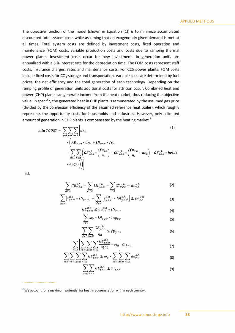
APPLIED METHODS


s.t.

The objective function of the model (shown in Equation (1)) is to minimize accumulated

discounted total system costs while assuming that an exogenously given demand is met at

all times. Total system costs are defined by investment costs, fixed operation and

maintenance (FOM) costs, variable production costs and costs due to ramping thermal

power plants. Investment costs occur for new investments in generation units are

annualized with a 5 % interest rate for the depreciation time. The FOM costs represent staff

costs, insurance charges, rates and maintenance costs. For CCS power plants, FOM costs

include fixed costs for CO2-storage and transportation. Variable costs are determined by fuel

prices, the net efficiency and the total generation of each technology. Depending on the

ramping profile of generation units additional costs for attrition occur. Combined heat and

power (CHP) plants can generate income from the heat market, thus reducing the objective

value. In specific, the generated heat in CHP plants is remunerated by the assumed gas price

(divided by the conversion efficiency of the assumed reference heat boiler), which roughly

represents the opportunity costs for households and industries. However, only a limited

amount of generation in CHP plants is compensated by the heating market.2

∑∑ ∑ [

(

∑ ∑ ( (

)

(

)

( )

( )))]

∑

∑

∑

(2)

∑[ ]

∑ [

]

(3)

(4)

∑

(5)

∑ ∑

(6)

∑ [∑ ∑ ∑

( )

]

(7)

∑∑ ∑ ∑

∑ ∑ ∑

(8)

∑ ∑

(9)

..............................

2 We account for a maximum potential for heat in co-generation within each country.

(1)


APPLIED METHODS


Total system costs are minimized, subject to several techno-economic restrictions: The

hourly demand within each country has to be met (Eq. (2)) and the peak demand

(increased by a security margin of 10 %) has to be ensured by securely available installed

capacities and net imports in the peak demand hour (Eq. (3)). Further important model

equations bind the electricity infeed and/or the construction of technologies. The

generation of a power plant is restricted by its availability (Eq. (4)) and the scarcity of the

used fuels (Eq. (6)), whereas the scarcity of construction sites limits the construction of

new power plant capacities (Eq. (5)). The hourly availability of dispatchable power plants

(thermal, nuclear, storage and dispatchable RES-E technologies such as biomass and

geothermal power plants) is limited due to unplanned or planned shut-downs e.g.

because of repairs, which are reflected in the parameter avd,hc,a in Equation (4). The

infeed of storage technologies is additionally restricted by the storage level of a

particular hour. Unlike dispatchable power plants, the hourly availability of fluctuating

RES-E technologies depends on meteorological conditions and varies on a very narrow

spatial scale. Hence, in the case of wind and solar power technologies, the parameter

avd,hc,a represents the (maximum possible) feed-in within each hour that is derived in

Section 4.3.3. Equation (5) depicts the space potential restriction for wind and solar

power technologies within a subregion. For other technologies, not the scarcity of space

but rather the scarcity of the used fuels is crucial. Equation (6) restricts the fuel use to a

yearly potential in MWhth per country, with different potentials applying for lignite, solid

biomass and gaseous biomass sources.

In addition to techno-economic restrictions, the electricity infeed and/or investment in

technologies can also be bound by political restrictions. Equation (7) states that the EU-

wide CO2 emissions in Europe's power sector may not exceed a certain CO2 cap per year.

Equation (8) formalizes an EU-wide (technology-neutral) RES-E quota as a percentage of

Europe's electricity demand. Besides EU-wide (technology-neutral) RES-E quotas,

national technology-specific RES-E targets can also be defined. Equation (9) formalizes

the politically implemented restriction that each country must achieve technology-

specific RES-E targets, as for example prescribed by the EU member states' National

Renewable Energy Action Plans (NREAP's) for 2020.

As such, the model is a profound tool to derive technically feasible and economically

efficient development pathways for Europe's power sector up until 2050. Specifically,

the effect of renewable energy technologies can be analyzed in an integrated manner.

4.3.2 Scenario Assumptions

In order to run the market model that was described in the previous section, calibration

is needed by defining all exogenous input parameters. To this end, a large number of

sources were deployed to create an appropriate set of assumptions, e.g. with respect to

the electricity demand level or the investment costs of the various technologies that

may be deployed. The following tables report the most important scenario assumptions

as they were used in the market model.


APPLIED METHODS


Table 4.4: Gross electricity demand [TWh] (Source: UoC)

Country 2011 2020 2030 2050

Belgium 102.60 116.13 116.13 130.24

Bulgaria 36.91 41.83 41.83 52.32

Czech Republic 73.71 87.96 99.00 123.83

Denmark 37.20 41.45 41.45 46.49

Germany 605.49 612.05 630.66 630.66

Estonia 9.79 11.06 11.06 13.83

Ireland 29.37 34.16 34.16 38.31

Greece 62.20 71.86 71.86 94.43

Spain 297.91 416.54 416.54 547.36

France 555.80 598.95 642.85 720.96

Italy 347.83 407.45 469.37 616.79

Latvia 7.01 10.00 10.00 12.51

Lithuania 10.93 14.00 14.00 17.51

Luxembourg 6.47 7.00 7.00 7.85

Hungary 44.21 52.40 52.40 65.55

Netherlands 124.94 135.85 135.85 152.36

Austria 66.40 77.53 77.53 86.95

Poland 155.84 202.36 202.36 253.10

Portugal 55.22 66.54 66.54 87.43

Romania 66.41 86.52 86.52 108.21

Slovenia 14.14 15.61 15.61 19.52

Slovakia 30.27 35.55 35.55 44.47

Finland 90.37 101.65 101.65 114.00

Sweden 160.30 174.18 174.18 195.35

United Kingdom 372.16 397.75 397.75 446.07

Switzerland 57.49 65.42 65.42 73.37

Norway 104.34 118.73 118.73 133.15

Sum 3525.31 4000.51 4136.00 4832.61

Table 4.5: Technology investment costs [€/kW] (Source: UoC)

Technology 2011 2020 2030 2050

CCGT 1250 1250 1250 1250

CCGT CHP 1500 1500 1500 1500

CCGT CHP CCS x x 1700 1600

Hard Coal 1500 1500 1500 1500

Hard Coal CHP 2650 2650 2275 2050

Hard Coal CHP CCS x x 2875 2600

Lignite 1850 1850 1850 1850

Lignite CCS x x 2550 2450

Nuclear 3157 3157 3157 3157

OCGT 700 700 700 700

Oil 800 800 800 800

Biomass gas chp 2600 2597 2595 2590


APPLIED METHODS


Biomass gas lc 2400 2398 2395 2390

Biomass solid 3300 3297 3293 3287

Biomass solid chp 3500 3497 3493 3486

CAES 850 850 850 850

CSP x 3989 3429 2805

Enhanced geothermal system

15000 10504 9500 9026

Geothermal high enthalpy 1500 1050 950 903

Hydro storage x x x x

Pump storage x x x x

PV ground 1532 1167 842 661

PV roof 1702 1297 935 734

Run of river x x x x

Wind Offshore 3100 2200 1900 1700

Wind Onshore 1250 1200 1150 1050

Table 4.6: Grid extension costs (Source: Energynautics)

Technology Costs

AC overhead line incl. compensation 445 €/(MVA*km)

DC overhead line 400 €/(MW*km)

DC underground 1250 €/(MW*km)

DC submarine 1100 €/(MW*km)

DC converter pair 150000 €/MW

Table 4.7: Fuel prices – based on the IEA World Energy Outlook [€/MWhth] (Source: UoC)

Fuel 2011 2020 2030 2050

Nuclear 3.6 3.7 3.7 3.9

Lignite 1.4 1.45 1.45 1.45

Oil 60.4 99 110 116

Coal 11.8 12.5 12.8 13.1

Gas 18.2 25.2 28.3 31.3

4.3.3 Typical Days

The challenge of integrating renewable energy technologies in a fundamental electricity

market model mostly stems from the non-dispatchable nature of wind and solar-based

power production that distinguishes them from conventional power plants. Weather

conditions vary on a narrow spatial and temporal scale that needs to be represented by

a sufficiently high spatial and temporal resolution in the model. In the modeling

approach developed in this study, these quantities are represented in typical days.


APPLIED METHODS


The use of typical days reduces the run-time of the model by reducing the temporal

resolution while maintaining the characteristic statistical features of the load and gene-

ration profiles. In this project, a tool was developed that derives up to 32 typical days

which capture the characteristic statistical features of an 8760 hour dispatch calculation,

such as mean values, seasonalities, gradients and interregional interdependencies.

During a model run, these typical days are scaled up to 8760 hours in order to represent

a full year of planning and operation. The typical days comprise the following parameters:

the hourly electricity demand profile per country depending on the day of the week

(weekday vs. weekend) and the time of the year (summer vs. winter) based on

historical hourly load data by [22] and

the hourly wind speed and solar radiation profile per subregion depending on the

level of wind speeds (strong wind vs. weak wind) and the time of the year (summer

vs. winter) based on historical hourly wind speed and solar radiation data by [1].

For a detailed description of the methodology that was developed in order to derive

typical days the reader is referred to [3].

In order to be used in the electricity market model, hourly wind speed profiles derived

for the typical days are transformed to hourly electricity feed-in profiles via so called

power curves. These curves report the average technical characteristics of the wind

turbines that are used in the model either today or in the future. To account for

technical improvement of the turbine design, power curves are assumed to widen over

the course of time thus making better use of a wider range of wind speeds. Note that

the electrical power output is expressed as percentage of the rated power (W/W installed)

which is important for the model as installed capacities are determined endogenously

during a model run. Power curves are based on [5]. For the specific case of onshore wind

turbines, power curves for 2011 and 2030 are depicted in the following figure.

Figure 4.3: Power curves for onshore wind turbines in 2011 and 2030 (Source: UoC)

0

0.1

0.2

0.3

0.4

0.5

0.6

0.7

0.8

0.9

1

0 5 10 15 20 25 30 35 40

Rel

ativ

e o

utp

ut

[W/W

inst

alle

d]

Wind speed [m/s]

Onshore 2011

Onshore 2030


APPLIED METHODS


In the case of photovoltaic systems, hourly solar radiation profiles derived for the typical

days are transformed to hourly electricity feed-in profiles via two steps. Due to the fact

that PV modules are tilted, in the first step solar radiation on the tilted surface is

determined based on geometric and optic considerations as presented in [6] and [7] and

solar radiation data for the horizontal surface. Hourly electricity feed-in profiles can then

be derived by the following equation that covers the technical characteristics of PV

modules:

(10)

where:

⁄

Similar to PV, a two-step calculation applies for concentrated solar power plants (CSP).

First, the direct radiation is derived [6], [7]. Then, the hourly electricity feed-in of the CSP

system is determined by its technical characteristics of transforming direct solar

radiation to electricity, as shown in the following formula:

(11)

where:

⁄

As in the case of wind power, hourly electricity feed-in profiles of PV and CSP systems

are expressed as percentage of the installed power (W/Winstalled) in order to later be able

to include endogenous PV capacities in a model run.

After having developed and calibrated the electricity market model, this part of the

project continues with two case studies in which the previously developed market

model is applied, both related to the impact of increased PV penetration in the

European power system. First, by iterating the electricity market model with an

household optimization model it is analyzed how the power system and PV deployment


APPLIED METHODS


develops when the levelized costs of PV electricity reach parity with retail prices (see

Section 5.5.2), thus incentivizing the inhouse-consumption of self-produced PV

electricity on the household level in Germany. Second, the market model is further

extended to include the transmission grid in a sophisticated manner, thus enabling to

optimize power generation and transmission infrastructures jointly through an iterative

approach based on power transfer distribution factors (PTDFs). The latter application

directly links the electricity market model to a physical model of the European power

transmission grid based on a well-defined interface (see next section).

4.4 COUPLING OF MARKET AND NETWORK MODELS

Electricity market models, implemented as dynamic programming problems, have been

applied widely to identify possible pathways towards a cost-optimal and low carbon

electricity system. However, the joint optimization of generation and transmission

remains challenging, mainly due to the fact that different characteristics and rules apply

to commercial and physical exchanges of electricity in meshed networks.

In this part of the project a methodology was developed that allows optimizing power

generation and transmission infrastructures jointly through an iterative approach based

on power transfer distribution factors (PTDFs). As PTDFs are linear representations of

the physical load flow equations, they can be implemented in a linear programming

environment suitable for large scale problems such as the one that was developed

within this project (Section 4.3). The algorithm iteratively updates PTDFs when grid

infrastructures are modified due to cost-optimal extensions and thus yields an optimal

solution with a consistent representation of physical load flows. The method is

introduced and demonstrated on a simplified three-node model in [App04]. As

described in the last section of this paper, the same algorithm is applied to a model of

the European power system in order to find the cost-optimal development of both

generation and grid infrastructures in the timeframe 2011 to 2050.

To this end, the market model that is introduced in Section 4.3 is first extended to

include the option of calculating power flows based on the PTDF representation. The

physical model of the transmission grid that was developed by Energynautics as

described in Section 4.2 is used to determine the PTDF matrices for the considered

years. Hence, the linkage between the models is established by the PTDF matrices, as

described in Figure 4.4.


APPLIED METHODS


Figure 4.4: Iteration scheme to jointly optimize generation and grid infrastructures (Source: UoC)

4.4.1 Market Model Specifications for the Model Coupling

In the market model, the spatial resolution is set to include 16 market regions, i.e. some

of the European countries (including Norway and Switzerland) are aggregated to larger

market regions. With respect to the temporal resolution, the model covers eight typical

days with four time slices each. A higher temporal resolution would have been desirable

in order to cover short term variations, e.g., in the load level or solar power generation.

However, the requirement of this study was to cover the entire European power system

with a sufficient level of detail for the spatial resolution. Furthermore, the inclusion of

the flow-based market coupling (based on PTDF factors) makes the optimization

problem very complex and hard to solve, as it establishes a tight interrelation between

many of the decision variables. Due to the tradeoff between a high spatial and temporal

resolution on the one side and manageable calculation times for solving the

optimization problem on the other, a compromise had to be found with respect to the

temporal resolution.3

The relatively low temporal resolution may result in an underestimation of flexibility and

balancing needs in the system. Therefore, the usage of flexible generation technologies

(particularly storage) as well as grid infrastructures may be underestimated. To address

this issue, the optimization algorithm includes a peak capacity condition, stating that the

peak demand needs to be met by securely available generation capacities including a

10 % safety margin (see Model description in section 4.3). As for the security of the

transmission grid, it can be argued that peaks in generation from renewable energies,

e.g. occurring during times of very high winds speeds, can be curtailed to avoid line

..............................

3 The optimization is solved on a PC with an Intel Xeon CPU 2.67 GHz processor and 96 GB RAM. Due to the

complexity of the optimization problem, the model needs approximately one week to solve.


APPLIED METHODS


overloading. Nevertheless, to further clarify this effect, the optimization based on an

improved temporal resolution but limited regional coverage is currently being prepared

and will be analyzed in an upcoming project.

As described in [App04], another challenge arises by the fact that each market region

spans several nodes within the grid model. To accurately capture the flows between the

nodes inside each region, which change depending on the dispatch of generation

technologies at any given time, node allocation keys (K) were introduced that represent

the distribution of the demand, the various generation technologies and the points of

connection for the DC lines within each market region. These allocation keys were

directly incorporated into the PTDF. In this way, the nodal power balances within the

load flow model can be determined for any dispatch situation, with the power flows

then following directly from the usual PTDF. Thus, the power flows on each line can be

calculated from the levels of demand (D), generation (G) and DC-Trades (TDC) as follows:

( ) (12)

Even though this approach allows calculating all line flows in a realistic manner, the

allocation keys represent a strong assumption as they exogenously define the

distribution of loads and generation within the market region. This means that the

model is not able to redistribute the capacities within a region in a way that might be

beneficial for the overall system. This becomes particularly important in Scenario 2

where a minimal level of grid extensions shall be determined. Note that this could be

overcome by simulating a nodal pricing regime where each node of the transmission

grid is its own market region. However, this would call for a market model that is even

more complex than the one that is currently used and could thus not be solved in a

reasonable time.

4.4.2 Network Model Specifications for the Model Coupling

The Power Transfer Distribution Factors (PTDFs) provide the linearized relationship

between the power balances at each node in the network model and the flows that

result on each of the transmission lines. They make up a matrix with as many rows as

there are lines in the model and as many columns as there are nodes. When this matrix

is multiplied with the vector of power balances at each of the nodes, the result is the

vector of active power flows on each of the lines which arise from a linearized (DC) load

flow. The PTDFs (also known as injection or generation shift factors) can either be

calculated directly from the impedances in the network (see Paper in [App04]) or they

can be calculated by measuring the change in line flow when a fixed amount of power

(say 100 MW) is shifted from some slack node to each of the other nodes in the network

model. For example, to calculate the PTDFs in the column corresponding to node X,

reduce the generation in the slack node by 100 MW, increase it by 100 MW at node X,


APPLIED METHODS


and measure the change in flow on each line in the model compared to the original

flows (using a DC load flow). As a fraction of the change in power (100 MW in this case),

this gives the per unit sensitivities for each line that make up this column of the PTDF

matrix.

Since the PTDF depends strongly on the impedances of the transmission lines, the PTDF

was recalculated for each iteration, based on the new line capacities calculated during

the optimization. These capacities were rounded up in 1500 MVA discrete steps,

representing a single 380 kV circuit, and then added to the network using standard

component models for the lines.

4.4.3 Robustness Test 1: Extreme Events

In the typical days used for the long-term European transmission and generation

planning optimization a variety of unusual weather events are represented, including

low wind and low sun. In addition to these day-long extreme events, the network and

generation capacities were also tested against a prolonged 10-day period with both low

wind and low insolation. The purpose was to demonstrate the robustness of the system

even under difficult conditions.

Figure 4.5: Availability of wind and solar power plants as a fraction of total installed capacity during the extreme event in Germany (Source: Energynautics)

The network and generation capacity results were taken from the optimization

described above (see Section 4.4) and then combined with wind and solar availability

data from a known extreme event from 5th through 14th January 1997, during which

wind speeds were poor and extensive cloud cover reduced insolation (see Figure 4.5).

The insolation data were taken from S@tel-Light [61] and the wind speed data from

NREL [62]. The wind speed was then converted to a power plant per unit of installed

capacity using a curve from [5] (see Figure 4.3).

Dispatch and demand data were taken at a resolution of two hours, so that in total 120

snapshots for the ten day period were considered. The whole system was then run

through a linear optimization routine, using DC load flow, to see whether all the load

could be covered under these extreme circumstances. Generation, storage and the


APPLIED METHODS


dispatch of HVDC lines were optimized at a nodal level, under the conditions that the

load was all met, that no lines were loaded over their thermal limits (66.5 % of their

total MVA capacity, assuming a 95 % power factor and 70 % factor for n-1 security), that

the storage was 70 % efficient (for the roundtrip of storing and then feeding energy

back) and that at the start of the event all storage devices were half-full.

If all the load could be covered without overloading, the dispatch of generation and

storage assets were optimized to reduce the maximum loading of the lines in the

network during the event. If all the load could be covered but some lines became

overloaded, the necessary expansion of the network was minimized so that all lines

were within their thermal limits.

4.4.4 Robustness Test 2: AC Checks

Energynautics' network model was further refined during this project to work for AC

load flow calculations (see Section 4.2.1), which in addition to real power flows in the

network, also take account of reactive power flows and thermal losses. All dispatch

situations from the long-term European planning optimization and half of those from

the 120 extreme event optimization dispatches were tested with AC load flows to make

sure no lines were overloaded, respecting n-1 security criteria, and that all voltage

angles were within stability limits.

The optimization of capacities described above in Section 4.4 was done using PTDFs

(also known as generation shift factors), which are essentially the same as a DC load

flows. It is necessary to use DC load flow for such large problems, in order to linearize

the load flow equations and thus make the problem amenable to linear programming

routines. While DC is a good approximation to the real AC load flow when the network is

well compensated for reactive power flows, some simplifications in particular situations

lose their validity:

For a line with only series reactance and voltage the same at both ends, the

active power flow is given by

where is the voltage angle. DC load

flow makes the additional simplification for small angles, which is not

always valid for large power flows on long lines with high impedance and can lead

to stability problems.

Reactive power flows cannot always be ignored. (In fact the power factor improved

between 2011 and 2050 as power flows increased and lines approached their

natural loading from below.)

Losses, quadratic with the current are neglected.

As a consequence of all these effects, the overall power flows, including active

power flows, can be slightly distorted, particularly in meshed networks.


APPLIED METHODS


In order to check the network model against these effects, each typical day and extreme

event snapshot was tested first for convergence of the non-linear AC load flow

calculations and then for overloading and angle stability.

To deal with convergence and stability problems when they arose, the load and

generation were uniformly reduced until convergence was reached, to see which parts

of the network were problematic. Overloading was fixed by expanding the capacity of

the lines. To deal with angle stability problems, lines were compensated with capacitors

in series. This has the effect of reducing the line's total series reactance and thus

enabling larger power flows without large voltage angles between buses and the

associated stability problems.

4.5 MODELS OF PV, STORAGE AND AN OFFICE BUILDING FOR DISTRIBUTION SYSTEM

To simulate the effects of high PV production in LV grids, models of the following

components have been developed: a PV plant model, a model of an electrical storage

unit and a model of a small office building. The models are developed to be able to

simulate the increased PV production effects on voltage variations in a distribution grid.

The models should also be useful in simulating distribution system power constraints

and methods for relieving high load cases.

The mentioned issues also determine the selected time scales used in the development

of the models. The step size of the simulations should be fast enough to give a good

representation of fluctuations, such as those induced by clouds passing over the PV

plant, but they do not go into higher detail, such as simulation of power electronics and

switching harmonics (Power Quality models are discussed in sections 4.6 and 4.7). The

steps should also be large enough to allow a simulation of large systems over longer

periods. Due to these restraints and preferences, the models are developed as power

sources in the simulation models.

Some of the models developed are driven by time series such as meteorological data

(solar irradiation and wind speed) and power consumption. These data can be either

measured or simulated. The meteorological data excite the dynamics of the models, for

example the wind and temperature are inputs to both the PV model and the model of

the office building. This dynamic input will then influence the models’ output and

designate their dynamic power output that affects the voltages in the distribution grid.

4.5.1 PV Models for the Distribution System

To study the impact of PV in the distribution grid two PV simulation models have been

developed in this project, the DTU and KTH models. The models of PV systems, including

PV panels and inverters, have been developed and implemented in MATLAB/Simulink

and DIgSILENT PowerFactory.

DTU modeled PV panels using a single-diode four parameters model based on the data

sheet values and the PV inverter is characterized by a power dependent efficiency. The


APPLIED METHODS


model uses meteorological measurements from a weather station as an input for the

solar irradiance, ambient temperature and wind speed. Furthermore the geographical

location and the current day and time of the simulation are needed as inputs to account

for the solar irradiance angle on the PV panels. The model then adjusts the input for

panel tilt angle, orientation and placement, the result is then run through the panel

model, where wind cooling is considered, and the inverter model to derive and AC

output. A detailed description of the model can be found in [App06] (see also [App05],

[App07] and [App08]).

The KTH simulation model only includes the PV system modeling but is also based on the

static generator component in PowerFactory and single-diode model. The purpose of

the KTH model is to create a model that can easily be implemented in distribution

systems and scaled to different ratings. The input to this model is the irradiation and

module temperature, simplified compared to the DTU model which also includes the

wind cooling effects and ambient temperature. The power output also depends on the

DC voltage and under these circumstances it is very important for the converter to have

DC voltage control to ensure operating at maximum power point. The maximum power

point (MPP) is the point at which system has the highest possible efficiency. The

maximum power point tracking (MPPT) function regulates the DC output voltage and

current in such a way that the maximum possible power can be obtained, with respect

to any changes such as changes in irradiation or temperature. For any condition there

can only be one operating point in the system with maximum efficiency, i.e. maximum

power output. An MPPT algorithm based on the method of Incremental Conductance

has been implemented in the PowerFactory simulation model. Four different

voltage/reactive power control algorithms have been implemented in addition to active

power curtailment based on over frequency or a trigger signal, for example if the system

frequency exceeds 50.2 Hz. The voltage/reactive power control is done through power

factor control, dynamic power factor control, droop based control and AC voltage set-

point control. A detailed description of the model can be found in [App11] (see also

[App12] and [App13]).

4.5.1.1 Aggregated PV Models

Aggregating PV systems in a PV plant is an important aspect for simulation and control

issues. PV plants are often composed of several individual PV systems that are

connected through transformers to the point of common coupling (PCC) to the MV or

HV grids. Instead of local voltage control, PV plants can be equipped with a voltage

regulator to control the voltage at the PCC. The aggregation needs to depend on

different aspects such as grid configurations, loads and PV characteristics etc. The

voltage regulation scheme also plays an important role and must be carefully considered

in aggregation studies.


APPLIED METHODS


4.5.1.2 Voltage Control in the Distribution Network

For voltage control one needs to investigate the controllability and interactions among

the PV systems. Analytical control methods can be used to evaluate the risk of negative

interactions between controllable devices that are electrically closely connected in the

system. This can be done through methods like relative gain array (RGA) and condition

number (CN). These methods can be used for the steady-state gain which is the

sensitivity matrix. Moreover, the characteristic of the sensitivity matrix is employed to

show the level of dependency of reactive power to active power for voltage control.

The RGA based method of the voltage sensitivity matrix is utilized as a quantitative

measure to address controllability and the level of voltage control interaction among PV

systems. The CN method is based on the Singular Value Decomposition (SVD) of the

voltage sensitivity matrix and is used as a mathematical measure to indicate the voltage

control directionality among PV systems. The term directionality refers to the direction

of the input vector, i.e. the active and reactive power change. This refers to different

amount and direction of power injections at the nodes. This means one can look at the

voltage change depending on where and how the active or reactive power injections are

changed.

Droop based voltage control methods, using reactive power, are more attractive in

voltage regulation through PV systems in LV grids as the risk of negative interactions is

low. Two coordinating methods applied for voltage control using reactive power are

developed. The droop control can depend on the voltage – Q(V) droop based voltage

(DBV), or depend on the injected active power – Q(P) active power dependent (APD). In

APD, the local required reactive power is determined based on the local feed-in of active

power of each PV system. In DBV, in contrast, local voltage is directly used as a measure

to attain the local required reactive power of each PV system. Though APD addresses

voltage indirectly, both methods aim to regulate the voltage to keep it under the steady-

state voltage limit using cost efficient feedback signals. A challenge is to design the

droop controls to achieve a good voltage profile in all operation conditions, share the

control burden between the PV systems and keep the losses to a minimum. New droop

based controls need to be compared with existing methods such as those imposed by

the German Grid Codes.

Furthermore, the voltage can be regulated by varying the active power. The use of

energy storage or load shifting may support voltage regulation. Methods are needed to

utilize the energy storage or make the load shifting in an efficient way, both from the

perspective of method efficacy and the economic point of view.


APPLIED METHODS


4.5.1.3 Validation of the PV Models

The model developed by DTU is validated against real measurements and the model

developed by KTH is validated against simulations with a detailed model in PSCAD.

In order to validate the developed DTU simulation model for a PV system, and to point

out the importance of considering the atmospheric conditions, such as temperature and

wind speed, and also the orientation and tilt angle of the panels, the simulations have

been compared with experiments carried out using SYSLAB – DTU´s experimental facility

for distribution grid research.4 A time series of measured solar irradiation, ambient

temperature and wind speed are run through the model to produce a time series of the

AC power output of the PV plant. The output is then compared to the output of the

actual PV plant in SYSLAB for that particular day to verify the model and to assess its

quality.

Figure 4.6 a) shows the ambient and PV panel temperatures and the influence of solar

irradiation (Ga) and wind cooling (Ws) on the PV panel temperature.

Figure 4.6 b) shows measured values compared to simulated values where there is no

adjustment for wind and ambient cooling, or panel tilt and orientation.

Figure 4.6 c) shows measured values compared to simulated values where adjustment

for wind and ambient cooling are added as well as the panel tilt angle.

Figure 4.6 d) shows measured values compared to simulated values where the final

adjustment for the 13° deviation from south has been added. As seen from the figure

the conformity between the simulated and measured values is quite good. The biggest

deviations are caused by shades of objects such as trees in the vicinity of the PV panels

which are not considered in the model. Further details of the model validation are

available in [App07].

..............................

4 SYSLAB includes three PV systems (one of 7.2 kW and two of 10kW) as well as a Vanadium Redox Battery

of 15 kW/120 kWh and an office building with controllable loads of a total of 10 kW.


APPLIED METHODS


a) b)

c) d)

The dynamic behaviour of the KTH model is validated using PSCAD. The PSCAD PV model

is a very detailed model which takes considerable time for simulation even for a very

small power system network. Even though the PowerFactory model is very fast, it

captures all the dynamics during disturbances in both the DC and AC side of the PV

system, just like the PSCAD model. Since the PSCAD is already a validated model, similar

response of the new PowerFactory model for the same disturbances validates the new

models credibility. Details can be found in [App11].

4.5.2 Model of a Storage Unit for the Distribution System

Increased distributed generation is becoming more important in the current power

system and in the future the system will rely more on DER components with energy

storage and on smart grids. The electrical power system is facing an evolution from the

traditional concept of energy generation by a few localized power plants interconnected

together through a meshed transmission system to distributed medium and small scale

generators. Some types of these generators embedded into the distribution network are

fed by renewable sources like sunlight and wind. Their main drawback is their partially

predictable behaviour and limited controllable output.

The battery package is an interesting option for storing excess energy from renewables

(related to the limited grid capacity) for later use. It may also act as a peak shaving unit

and thereby contribute to decreasing loading on the grid. The presence of energy

storage systems may allow a better management of the electric system, thus allowing

Figure 4.6: Influence of ambient temperature, wind and orientation on the PV model (Source: DTU)


APPLIED METHODS


for the full exploitation of renewable energy sources. Distribution companies have

started to recognize that storage has the unique ability to act as a buffer between the

grid and generation that is either intermittent or not controlled by the utility.

Vanadium Redox Batteries (VRB) have many advantages compared with other storage

technologies. These include a high storage efficiency, low maintenance cost and long life

cycle. The vanadium battery system (with a nominal storage capacity of 120 kWh)

installed in SYSLAB is connected to the grid via a four quadrant power converter and can

deliver 15 kW on the AC side. Figure 4.7 shows a picture of the system during installation

and a list with the main system components. The battery can operate in two modes:

P-Q mode (where the active and reactive power of the battery are set by the user) and

U-f-mode where the power is varied in order to control grid voltage and frequency using

pre-defined droop-curves.

Figure 4.7: The Vanadium Redox battery in SYSLAB during installation and its system components (Source: DTU)

In order to study various aspects of battery storage systems, accurate dynamic battery

models are required.

The Vanadium Redox Battery (VRB) system model developed at DTU is based on the

equivalent electrical circuit and on power balance between the input and the stored

power considering the efficiency of different components, such as: cell stacks,

electrolytes, pumps, power converter and the power losses. These characteristics of the

battery have been calculated by measuring different electric values at different loads

and state of charge levels.

The model for the vanadium redox battery is verified by running time series of power

output and input to the battery through the model. The modelled state of charge is then

compared to the state of charge of the battery in SYSLAB to assess the quality of the

model.

System components:

Cell stacks (3x40 cells in total)

Electrolyte tanks (2x6500 liter)

Balance of plant (pipes,

pumps, etc.)

Control and communication

unit

AC/DC power converter


APPLIED METHODS


4.5.3 Model of an Office Building

The office building model is based on a small office building, FlexHouse at SYSLAB that is

heated by 10 electrical heaters of 1 kW each which can be used as a controllable load in

the system. The model for the building is formulated as a one room lumped-RC-model in

accordance with the commonly used thermal-electrical analogy. The model parameters

are then derived from physical knowledge and experimental data is then used

statistically to estimate the parameters in the model.

The FlexHouse voltage controller is based on a thermostatic control for the building, so

that when the temperature inside is below a certain set-point the heaters are turned on

and when the temperature is above another set-point the heaters are turned off. Using

flexibility provided by the building’s thermal capacity the heaters are also controlled so

that the voltage of the bus-bar is under a certain level when the PV production

increases.

To validate the model of the office building, the model uses the outdoor temperature as

an input to model the indoor temperature. A simple thermostatic controller is used to

control the heaters in the building to maintain a desired indoor temperature. The

simulated power consumption and indoor temperature are then compared to the

measured values for SYSLAB´s office building to validate the model.

4.5.4 Model of the Distribution Grid

For modelling of the grid, standard models for steady-state and EMT simulations

implemented in PowerFactory are used.

The distribution grid model is validated by simulating different grid configurations and

load cases and comparing the simulated voltages with measured voltages from SYSLAB´s

distribution grid. To verify the cable models with parameters defined from the data

sheets, two different types of tests using different configurations have been carried out:

a short-length test and a long-length one with a dump load or a battery connected to

the grid. The results have shown a good alignment between simulations, using power

flow calculation, and measurements.

4.6 METHOD USED FOR HARMONIC DISTORTION MODELING

Harmonic interaction studies can be done in the time domain, frequency domain, or as

hybrid calculations [23], [24].

Time domain calculations use differential equations, and therefore require detailed models

of power electronic devices, including the control algorithm of the PV inverter. With a

detailed model of a device, they are known to be very accurate when predicting behavior in

different conditions. Examples of studies done in the time domain are given in [25]-[28]. A

restriction of time domain calculations is that they are difficult to do for systems with a large


APPLIED METHODS


number of different units. Including the control algorithm of several different devices can be

a problem or even impossible, since their control algorithms are not always available.

Calculations in the frequency domain are widely used for harmonic studies. Sources of

harmonic currents are represented as ideal or non-ideal current sources, or the current

is determined from a look-up table based on the voltage of the busbar. As [24] suggests,

a harmonic source can also be represented as voltage source with a series impedance,

or as a current source dependent on the system impedance (current re-injection), which

emphasizes the effect of the system impedance on the current of the source.

Several types of calculations are proposed in the frequency domain [23], [24]: current

source method, power flow method, and iterative harmonic analysis. Examples of

studies in the frequency domain are given in [29]-[33]. More details about all methods

can be found in [34] (given also in [App23]).

Harmonic power flow method uses a Newton-type algorithm to solve current and

voltage equations at the same time for a single frequency. This allows the harmonic

current sources and other elements to be voltage dependent, and gives more accuracy.

On the other hand, the calculation becomes more complicated than the current source

method. A number of software tools use this method for harmonic analysis of the system.

Iterative harmonic analysis is an advanced version of direct and power-flow calculations.

The original methods are supplemented with voltage dependent current sources, and

sometimes even the frequency coupling. The direct matrix or power-flow simulation is

initially executed with assumed voltages on busbars of non-linear elements, resulting in

initial harmonic current values. These voltages are then compared with calculated

voltages for those busbars, and if needed, the calculation is repeated with new values

for current sources. This iterative procedure is repeated until the voltage changes on

busbars are within the desired error margins. The accuracy of these methods is

dependent on the complexity of models used. When detailed models of all elements are

used very accurate results can be achieved, but on the other hand the models require a

lot of parameters, which sometimes make them difficult to implement for complex systems.

To reduce the model complexity, a behavioral Norton equivalent model was adopted in

this report, which can represent the harmonic source in only one or few different

conditions (voltages). Another property considered is the equivalent linear impedance of

inverters, seen on the output terminals, which can interact with other impedances in the

network and possibly lead to local increases of harmonic voltages. The model

parameters were calculated from laboratory experiments conducted on several

commercially available PV inverters.

Frequency dependent impedance of the system is important for harmonic interaction

studies. Harmonic voltages are often increased due to a resonant or near-resonant

condition, and therefore attention should be given to the effect of impedance of PV

inverters. Other nearby equipment, such as power factor correction capacitors, should

be taken into account.


APPLIED METHODS


In this report, an analytical study on the distribution system harmonic impedances was

done, to investigate the uncertainties made by adopting different assumptions in the

modeling process.

In the case of multiple inverters connected to the system, an aggregated model can be used

to substitute the effect of all units. Summated current can have a maximal value equal to the

arithmetical sum of individual currents, but due to the phase angle diversity of individual

currents the sum is usually lower than that. Technical reference [35] suggests using a

generalized summation law for determining the total harmonic current of random loads:

√∑

(13)

where β is the summation coefficient with a value of 1 or greater, depending on the

harmonic order. General considerations about the summation of random currents are

given in [35]-[38]. Examples of aggregated models of PV inverters are given in [39], [40].

Reference [39] presents measurement results in which β had a value of approximately 1

(arithmetic summation) for harmonic orders up to 17, and a value of approximately 2 for

higher orders.

For the purpose of this report, a field measurement was conducted to determine the

empirical coefficient β which could be used for aggregating a group of PV inverters into a

single harmonic current source.

More details on the methodology of harmonic modeling can be found in [41] (given in

[App19]; see also [App17]).

4.7 METHOD USED FOR VOLTAGE DIP STUDIES

For voltage dip studies, a dynamic Matlab/Simulink model of an inverter was developed.

Since different manufacturers have different algorithms for fault ride-through, an “idealistic”

control of power was used in the model, which allows the inverter to react already in the

first period of the voltage dip. In reality, the inverter would need to ramp its reactive current

during several cycles of the voltage, which would result in a slightly slower response.

For this type of studies there is also a problem of generalizing parameters for different types of

inverters, in this case in a dynamic time-domain model. To avoid this problem, a simplification

was made to use a constant PQ source as the inverter model during a voltage dip, limited to

the nominal current of the inverter. Such a model could be used in a short-circuit calculation,

which approximates all network elements with their short-circuit equivalents.

The resulting model doesn’t describe the reaction time of the inverter, which is different

for different types, but it can generalize inverters to estimate the remaining voltage

during a dip and estimate their voltage support.

In the future, this approach should be validated by laboratory experiments.

More details about the short-circuit model can be found in [42] (also given in [App18]).


5 KEY RESULTS

KEY RESULTS


5. KEY RESULTS

5.1 POWER VARIATIONS FROM PV

5.1.1 Smoothing Effects

5.1.1.1 Large-scale

Section 3.1.1 elaborated on how geographical distance smoothes the output of PV. It

also discussed that variability is a function of time and space, i.e. given a certain spatial

dimension of the plant the cloud does not cover the complete area at the same time.

Factors influencing variability besides plant characteristics include cloud size, speed and

direction of movement, opacity and height relative to the PV plant, among others [63].

In a work conducted in the USA it has been established that the larger the plant, the

longer the time scale for the plant output to become identical to that of the output of an

irradiance meter measuring at a single spot [48]. PV plants with capacities in the tens of

megawatts, for example, show similar output as the irradiance meter if the comparison

time scale is chosen to be longer than 10 minutes. This means that below 10 minutes

the output of the plants is smoother than that of the meter due to the size of the plant,

as compared to the meter which experiences a very rapid change. For smaller plants this

time scale is lower. In a 30 kW plant, ramps longer than one minute are the same for the

plant and the meter. However, the smoothing on the plant level is visible on a higher

resolution of 1- and 10-seconds. As can be seen, these smoothing effects increase with

the plants’ size and are dependent on time scale. This analysis shows that it would not

be proper to take an output of a single plant and simply scale it in order to quantify the

output of several hypothetical plants separated by a certain distance from each other.

These considerations apply for the system level perspective. There are also issues of

localized concern, especially voltage and power quality issues in the distribution

networks which are discussed in chapter 3.3.

These considerations of one single plant can be easily transferred to an urban or a rural

area where a number of PV systems are dispersed across a large territory. The larger the

territory, the smaller the variations seen by the system operator and the less balancing

requirements are needed, which would significantly decrease the balancing cost. Also,

forecasting for a larger area can be done with higher precision as variations of individual

systems are eliminated. This is also where the electricity grid plays an important role as

it enables balancing between several regions.

Besides the variations in PV output it is important to consider possible correlation with

the demand in certain weather-induced situations. In a southern state of the USA an

observation was made that following a squall-line-induced drop in PV production the

demand in that particular area decreased as well due to the reduction in cooling load


KEY RESULTS


[63]. Besides being fairly predictable, this correlation can be expected in summer

months and decreases the amount of additional resources needed to compensate for

the reduced PV generation. This does not apply to cumulus-type clouds though, as load

is practically unaffected by these.

We compared insolation in hourly resolution at several distinct locations in Italy based on

measurement data from a geostationary satellite and estimated cloud cover [61] to see

the effect of smoothing across these locations. The 14 locations are spread across Italy and

hence quite distant from each other. Figure 5.1 on the left shows the insolation over the

day at 14 individual locations. As can be seen, there is some correlation at certain

locations, which must be affected by the same weather pattern. On the other hand, there

are anticorrelated values between some other nodes. If averaged across all locations, the

result is a very smooth curve, as can be seen on the right graph. This emphasizes that

pooling on a very large scale leads to a smooth insolation curve that would translate into a

smooth PV production curve. This means, for example, that the transmission system

operator responsible for the balancing reserves in the complete area would not be taken

by surprise by frequently and randomly changing ramps. This also shows that increasing

the size of the balancing area would help decrease the total required reserves.

Figure 5.1: Insolation at 14 distinct locations in Italy (left) and the average over the 14 locations (right) on a specific day in winter (Source: Energynautics)

5.1.1.2 Small-scale

At the DTU Risø Campus, three PV plants are connected to the experimental power

system facility, SYSLAB. The three plants are distributed approximately 250 to 450

meters apart and range from 7 to 10 kW in production capacity. The three plants also

differ in panel tilt and orientation with site 715 having an orientation of 190°, a tilt of 60°

and nominal power of 7 kW. Site 319 has an orientation of 180°, tilt of 40° and 10 kW

nominal power. The third site, site 117, has an orientation of 100° a tilt of 20° and 10 kW

nominal power.


KEY RESULTS


The variation over the day of the maximum power from the three PV plants is presented

in Figure 5.2. For comparison, the power outputs from each PV plant and for the

aggregated value are presented as normalized power relative to the maximum power

during the day. The three plants have different profiles during the day due to their

different orientations and tilt-angles.

Detailed examples of the power fluctuations are presented in Figure 5.3 around 10

o’clock with passing clouds causing dips in power generation, and in Figure 5.4 around

12 o’clock with passing holes in the clouds causing spikes in power generation.

Figure 5.2: The hourly maximum power for the three PV installations over the day (Source: DTU)

Even with the relative short distances between the PV plants, it is very clear that the

power fluctuations to some degree are uncorrelated, reducing the relative fluctuations

of the aggregated power.

Figure 5.3: Details of power dips. (Approx. 1 minute between the time marks) (Source: DTU)


KEY RESULTS


In Figure 5.3 around 09:56 a cloud passed over PV plant 117 without affecting PV plant

319 and PV plant 715. Around 09:59 other clouds passed over PV plant 715 and to some

degree PV plant 319, but with almost no impact on PV plant 117.

Figure 5.4: Details of power spikes. (Approx. 1 minute between the time marks) (Source: DTU)

In Figure 5.4 around 12:05 holes in the clouds are passing the PV plants, resulting in

large, but to some degree uncorrelated fluctuations. The relative fluctuations of the

aggregated power (the power to the grid) are a lot less.

A distribution of PV plants over only 1 km will have a significant impact on the rapid

power fluctuations of the aggregated power generation from the plants caused by

passing clouds. See the paper in [App10] for some further details.

5.1.2 Ramp Rates

The ramp rates have been studied based on several literature sources described in detail

in [App24]. Here the key statements are reproduced.

Concerning changes on the time scale of a single minute, the literature suggests the

following. With cumulus clouds a 10 km2 service area must be prepared to lose 15.9 % of

PV over an interval of 1 minute. This number decreases to 5.5 % as the size of the

service area is increased to 1,000 km2, whereas a 100,000 km2 area would lose 2.7 %

(results obtained through simulations).

Most 1-min-power changes lie within 10 % of capacity (67 systems in three service areas

were studied). 95 % of 1-min step changes are below 10 % of capacity (31 systems in

one service area were analyzed). 1-min step changes are within 40 % of capacity for an

area totalling 1.6 MWp, and within 20 % for an area totalling 25 MWp (consisting of 17

subsystems within a larger system). 99.7th percentile drops to 0.09 for 23 sites at 1-min


KEY RESULTS


resolution (with monitored radiation data for one year for 23 sites and distances

between sites from 20 to 440 km).

A squared-shape service area of 10 km2 with uniformly dispersed PV generation would

take 1.8 minutes to lose all of its PV generation as a consequence of an incoming squall

line. A larger service area of 100 km2 would take 5.5 minutes.

Concerning 10-minute changes, the following can be stated based on the literature

research. For most distributed fleets 95 % of 10-min step changes are below 10 % of

capacity (judged by electricity production from 31 systems in one service area). 10-min

step changes similar for the areas totalling 1.6 MWp and 25 MWp are within 40 %. The

maximum 10-min step change is between 90 and 100 % for all systems (judged by

electricity production from 8 individual systems).

Concerning 1-hour changes some results are as follows. 1-hour step changes are similar

for areas totalling 1.6 MWp and 25 MWp (within 40 %). The variability ratio is nearly

100 % for time scales longer than 1h (analysed based on six sites, with distances

between sites up to 3 km).

Some additional results concerning the impact of the PV modules’ orientation on the

ramp rates can be found in [App22].

5.2 ROLE OF THE ELECTRICITY GRID, STORAGE AND DSM

5.2.1 CAES Potentials

Due to the fluctuating nature of weather-dependent renewable energy technologies,

the integration of high shares of fluctuating renewable energy sources into the

electricity system necessitates additional flexibilities. On the supply side, one promising

future technological option related to flexibility is compressed air energy storage (CAES).

The basic concept of CAES involves using off-peak electrical energy (from renewable

sources such as wind and solar power or excess output of power plants) to compress air,

which is then stored at pressure underground. During periods of peak demand the

compressed air is released through a turbine to generate electricity.

In this study a systematic review of relevant literature on the potential of CAES in

Europe was performed. The main results can be summarized as follows:

The storage of compressed air can take place in porous rock formations (aquifers or

depleted oil/gas fields) or in large voids such as salt caverns or former mine works [8].

Several regions in Europe with underground storage formations (such as salt caverns)

are suitable for the construction of CAES facilities. [10] provides some information on

the location of geological salt deposits and salt cavern fields in Europe. As shown in

Figure 5.5, favorable ground formations for the construction of CAES facilities are

primarily located in Poland, Germany, Denmark, the Netherlands, the United Kingdom,


KEY RESULTS


France, Spain and Portugal. However, due to the fact that salt caverns are also suitable

for the storage of natural gas, the problem of competing uses arises.

In contrast to the storage of natural gas the problem of competing uses is less

pronounced with regard to the storage of carbon dioxide (CO2). CO2 storage demands

other geological characteristics and the storage occurs at greater depths (800 meter and

more) which usually lie under the level of the salt caverns. However, CO2 storage

requires a large area and salt caverns that lie right on top of such CO2 storage depots

could potentially not be used for CAES facilities [9].

Figure 5.5: Underground salt deposits and salt cavern fields in Europe (Source: [10])

Due to the problem of competing uses, the exact potential of CAES in Europe is hard to

quantify. As a consequence, quantitative estimations are rare. For Germany, quantitative

estimations of the CAES potential (useful energy) in suitable geological formations in the

North German lowlands amount to between 2.5 and 3.7 TWh [12], [11]. In addition, [3]

provides quantitative estimations of the generation potential (TWhel) of advanced

adiabatic compressed air energy storage (AA-CAES) in salt caverns in selected European

countries (however, not considering competing usages in terms of e.g. gas storage).


KEY RESULTS


Figure 5.6: AA-CAES generation potential (Source: [3])

Besides underground CAES facilities, there are also projects for small-scale CAES facilities

that store air in fabricated high-pressure tanks which are independent from geological

formations. However, the capital and production costs of such small-scale CAES facilities

are much higher than the costs of large-scale CAES facilities (which use geological

formations such as salt caverns) [13].

5.2.2 Impact of the Electricity Grid and Storage on PV Utilization

Section 3.2 described how the transmission system, storage and DSM all complement

each other in facilitating the integration of large amounts of PV into the electric system

and increasing its share in supplying the system demand.

Energynautics conducted a simulation study that aims to quantify how much PV is

actually feasible in the system on a European level from the perspective of enabling high

utilization of this resource, that is, making sure that there is only minimal curtailment of

PV. Limitations due to limited transmission network and storage5 capacities are a focus

of this study. For the study, Energynautics’ European Transmission System model built in

DIgSILENT PowerFactory was used (see section 4.2).

..............................

5 Only short-term storage such as household battery systems, electric vehicles, pumped hydro power and

compressed air energy storage were considered as opposed to long-term storage options such as power-

to-gas and hydrogen.


KEY RESULTS


In this section, a brief summary of the methodology and results of the study are framed.

An interested reader is invited to view the complete study including a detailed

description of the methodology in the annex of this report [App02].

The principal question aimed to be answered in this study is how efficiently power

available from PV installations can be utilized on the European level. This depends on

how much power generated by PV is consumed locally on the individual nodes of the

transmission network, how much of the excess power can be transported to other

locations and how much power can be stored provided storage capabilities are in place.

Several projections concerning the installed capacity, starting with the base case, are

considered with the goal to increase PV’s share in supply of the demand.

Simultaneously, more PV capacity may lead to large amounts of local excess PV power at

certain locations in the system in certain hours in relation to demand on the same

nodes. The limitations for power exchange between distant regions by means of the

transmission system, given by the limited thermal capacity of transmission lines, lead to

curtailment of PV power.

5.2.2.1 Methodology

In the first step, suitable locations and appropriate capacities for PV installations are

identified for the base case under the assumption that demand is supplied completely

by PV for a specific hour. In order to have PV benefit from locations with best irradiation

conditions, placement of generation capacities was carried out in accordance with

region-specific average annual solar insolation data using a DC optimal power flow

calculation. The resulting installed PV capacity in Europe totals 770 GWp. This number

represents the base case to be used for simulations of the complete year. PV plants

consist of both small and large PV systems situated at all voltage levels underlying the

corresponding node in the transmission network.

After the base case installed PV capacity is determined, in the second step a complete

year is calculated for the determination of utilized and curtailed PV energy while

considering different scenarios in terms of available storage capacity. The base case PV

capacity of 770 GWp was scaled up in several steps and each time calculations of a

complete year using demand and irradiation data for Europe in hourly resolution were

performed, which enabled a quantification of the lost PV energy due to missing demand,

transmission capacity and storage.

In terms of available storage capacity three scenarios were defined. In scenario 1 no

storage was considered, thus removing the possibility to capture PV power that is

curtailed owing to restrictions imposed by the thermal capability of the lines or lack of

demand. This is the most pessimistic scenario and leads to the highest amount of

curtailed PV. In scenario 2 storing PV energy was allowed in today’s pumped hydro

power plants, whose locations are known and are placed on the corresponding nodes in

the model. In addition, some extra storage was added at nodes that exhibited PV


KEY RESULTS


curtailment after whole-year calculations according to scenario 1, with installed PV

capacity determined from the base case (770 GWp). In this scenario the total storage

capacity adds up to around 290 GWh. Last, scenario 3 incorporated storage that was

dimensioned and placed in accordance with PV curtailment as seen in the year

calculated in scenario 1 having around 1155 GWp PV in the system. Clearly, the resulting

amount of storage capacity of about 1540 GWh is substantially higher than the one

derived from calculations with 770 GWp PV installed in Europe. Table 5.1 gives an

overview of the considered scenario settings. As can be seen from the table the number

of conducted whole-year calculations adds up to 12.

Table 5.1: Calculation scenarios (Source: Energynautics)

Installed PV, GWp Total storage capacity in Europe in GWh

Scenario 1 Scenario 2 Scenario 3

770; 1155; 1540; 1925 none 290 1540

5.2.2.2 Results

In scenario 1 the unavailability of storage means that the only way to avoid curtailment of

PV that is present in abundance at one node is to transport it away by means of the

transmission grid. The maximum transportable power is limited by the thermal capacity of

the network. Figure 5.7 shows the relevant results in dependence on the total installed PV

capacity in Europe. Starting with 770 GWp of installed PV, less than 1% of annual PV

energy available in abundance at certain nodes cannot reach other locations to be utilized.

In this case PV is able to supply around 17% of the yearly load. As the installed PV capacity

increases by 50% to 1155 GWp, curtailment can be seen to have increased to over 6% in

total, and the largest part of it is caused by the grid restrictions. However, there are some

hours in a year now where the total energy available from PV exceeds the total amount of

load in the system such that the surplus amount could not be consumed even if the grid

were not the limiting factor, and is therefore ascribed to missing load. This quantity grows

further with increasing PV capacity and at some point shortly after 1700 GWp, PV curtailed

due to missing load exceeds the amount of curtailed energy caused by grid restrictions.

The latter share exhibits a saturation behavior staying relatively constant at 10% of total

available PV energy from about 1550 GWp on. This means that up to this amount of

curtailed PV could be saved by enforcing the grid appropriately. If the installed capacity of

grid-connected PV systems should reach 1925 GWp without appropriate grid enforcement

or storage options, 25% of available PV energy would be wasted. The PV’s share in load

coverage does not follow the proportionality of increasing installed capacity and thus only

supplies about 32% of demand with 1925 GWp installed as compared to 17% being

supplied by a 2.5 times smaller capacity of 770 GWp.

In scenario 2 with 290 GWh available storage capacity the two factors that influence the

amount of curtailed PV energy, namely the grid restrictions and excess of PV energy in


KEY RESULTS


relation to demand in the system in certain hours, are simultaneously fixed. Figure 5.7

illustrates the quantities related to PV usage in this scenario. As can be seen, storage

introduced into the system is now able to reduce the amount of curtailed PV energy to

around 23% compared to 25% seen in scenario 1 for 1925 GWp of installed PV. This seems

to be a modest number, however the absolute amount of avoided curtailed energy still

adds up to nearly 51000 GWh per year, which corresponds to the electricity consumed by

Portugal in 2011 [64].

Larger storage in scenario 3 (1540 GWh) is able to capture almost the complete excess

PV energy up until 1155 GWp of installed PV. It also significantly contributes to

reduction of curtailed PV energy caused by grid restrictions. With 1540 GWp PV in the

system the curtailment totals to 5%. In the end, with 1925 GWp present in the system

the PV’s share in load supply adds up to about 38% under a curtailment of about 12%,

which is mostly attributed to grid restrictions. In the present case appropriate grid re-

enforcement would contribute significantly to reduction of the total curtailed PV energy.

Summarizing, the results show that even about 2000 GWp of PV in the system could be

feasible provided that the grid is expanded in appropriate locations so as to enable the

transport of abundant PV energy at some nodes to others where this resource is scarce.

A large damping effect is provided by strategically placed short-term storage with a total

capacity across Europe of 1540 GWh. It can thus be concluded that around 30 to 40% of

Scenario 1: no storage

Scenario 2: 290 GWh of storage

Scenario 3: 1540 GWh of storage

Figure 5.7: Whole-year calculation results for scenario 1, 2 and 3 (Source: Energynautics)


KEY RESULTS


annual demand in Europe can be feasibly covered by PV. With this number, the amount

of curtailed PV energy is acceptable in relation to the amount of short-term storage that

needs to be built. Any further expansion of PV capacity is likely to represent a high

economic burden owing to the disproportionately high amount of required storage capacity.

5.3 ISSUES IN THE DISTRIBUTION NETWORKS

5.3.1 Voltage Variations in Distribution Networks due to PV

For voltage control at the distribution network level one needs to investigate the

controllability and interactions among the PV systems. Two analytical control methods

are investigated, namely Relative Gain Array (RGA) and Condition Number (CN), using

the voltage sensitivity matrix in order to find the degree of controllability. Although RGA

was introduced for pairing input and output variables in a decentralized control system,

it has also been exploited as a general measure of controllability. RGA is basically

defined as the ratio of the open loop gain between two variables in a Multiple-

Input/Multiple-Output (MIMO) system to the closed loop gain of the same variables

while other outputs are perfectly controlled. RGA has been addressed in many literature

sources and frequently employed as a quantitative measure of controllability and

control loop interaction in decentralized control design.

The results show strong interactions between the voltage control of buses in a radial

system, especially at high R/X ratio. Decentralized voltage control to specific set-points

through reactive power regulation or active power curtailing is not feasible in the LV grid

due to strong interactions indicated by large RGA elements and large CN of the voltage

sensitivity matrix. Strong interactions can be attributed to the system topology, often

radial in LV grids. Another important factor is the R/X ratio where a higher ratio

decreases the reactive power influence on the voltage. Instead, active power has a large

influence on the voltage. It is furthermore shown that using decoupling controllers to

make the system decentralized must also be avoided, as the RGA elements of the

voltage sensitivity tend to be larger than 5. Such control could result in poor control

performance. Instead, droop based control and coordination can efficiently keep the

voltage under a specified limit in the LV grid.

5.3.2 Voltage Control Issues / Coordination of PV

Voltage control is becoming more important in distribution grids, as PV feed-in changes

the voltage profile along the feeder. When the PV production increases, overvoltage

problem may occur and can be dealt with by reactive or active power control. The

previous section described the influence on the voltage from a change of reactive or

active power in a node using the voltage sensitivity. For proper voltage control,

coordination is needed in the control design. Methods have been developed to deal

with over voltages by reactive or active power control. The reactive power coordinated


KEY RESULTS


control methods are droop based on either active power or local voltage measurements.

The voltage control methods using active power are based on load shifting or energy

storage.

5.3.2.1 Voltage control by reactive power

Two general methods for local voltage regulation are developed which utilize the

voltage sensitivity matrix and are based on coordination. These two methods are the

Active Power Dependent (APD) and

Droop Based Voltage (DBV).

In APD, the reactive power required locally is determined based on the local feed-in of

active power of each PV system. The voltage sensitivity matrix is used to propose an APD

method that can locally coordinate setting parameters in the control method Q(P). The

voltage regulation in the proposed Q(P) method can generally be done in two ways,

regulating either last-bus voltage in a radial feeder or regulating the voltage profile of a

radial feeder through connected PV systems. When the PV system production reaches a

predetermined operating set-point, voltage regulation starts. There is, therefore, no

reactive power consumption by the PV systems prior to the operating set-point. The

information of the voltage sensitivity matrix is employed to locally determine the gain

relation between reactive power and active power of a PV system with respect to the

operating set-point. In other words, the reactive power of each PV system is locally

regulated in accordance with its active power output and with respect to the

predetermined operating set-point in order to regulate the voltage. The steady-state

voltage profile limit is used to determine the operating set-point. The Q(P) methods or

in general APD methods do not directly consider the voltage. The voltage is indirectly

addressed. It comes down to the fact that the required reactive power at each PV is

based on the PV production, regardless of the voltage. This issue can be considered as a

shortcoming in APD methods because when the demand and the PV production are

simultaneous, the voltage rise does not happen so that reactive power production is not

necessary. Alternatively, instead of measuring the power production of the PV system,

the total net production/consumption in each node may be used to improve the control

performance. The node consumption, thus the net power production, varies depending

on several parameters such as time and day of the week etc. mostly independently of

the PV production. The simplicity and performance speak in favor of the APD method.

In DBV, in contrast, local voltage is directly used as a measure to attain the local

required reactive power of each PV system. Coordination of droop parameters among

several PV systems is a challenge on the grounds that PV systems at the beginning of a

radial feeder participate less in the voltage regulation compared to those at the end

which experience the voltage rise. A coordinated control method Q(V) is proposed that

locally determines the Q(V) setting parameters based on the voltage sensitivity matrix.


KEY RESULTS


Though APD addresses voltage indirectly, both proposed methods regulate voltage in

such a way to keep it under the steady-state voltage limit using cost efficient feedback

signals. Different possible aspects of the developed methods are discussed in this study.

Aggregated or equivalent models are simulated in several scenarios to validate the

possibility of replacing several PV systems by an aggregated model. The conclusion of

this study is that, although the reactive power operation modes of individual PV systems

in a non-aggregated model might be different (capacitive or inductive), the performance

of the voltage regulator in both aggregated and non-aggregated models would be

similar. In the dynamic sense there are some differences, depending on the scenario. For

the dynamic response it would be possible to tune the parameters in the aggregated

model to achieve similar response to the non-aggregated models. The voltage regulation

scheme also plays an important role.

An aggregated model for PV systems using APD control is straightforward whereas DBV

needs more care.

For the detailed results of the studies please refer to [App14], [App15] and [App16].

5.3.2.2 Voltage control by active power

An efficient way of controlling the voltage in a distribution network is to control the local

power consumption at the bus-bar. The consumption can be influenced by:

Shifting load or

Using energy storage.

The ability to control active units can reduce the stress on the low-voltage grid by

consuming the PV energy production locally. Home energy management systems, such

as the SMA Sunny Home Manager, can increase the share of PV energy being consumed

at the distribution customer’s site. Thus decentralized consumption is increased and the

stress and losses in the grid are reduced.

To test different voltage controllers, the simulation models developed and implemented

in PowerFactory (presented before in sections 4.5.1 (PV) and 4.5.2 (VRB)) were used.

Additionally a model of a small office building is used [App09]. The model allows for

simulation of the indoor temperature of the building using ambient environment

measurements and heat input from ten 1 kW electrical heaters. The building is modelled

as one large room where the heat flow is modelled with a grey-box approach, using

physical knowledge about the heat transfer together with statistical methods to

estimate the model parameters. Finally a model of a small distribution system has been

developed for the simulations. The model is based on SYSLAB´s cable network and uses

datasheet values for the actual cables used in the laboratory (see section 4.5).


KEY RESULTS


Voltage control by load shifting

Using the model of the office building in SYSLAB a controller for load shifting has been

developed. The controller uses the electrical heaters in the office building to either

reduce or increase the local grid voltage turning the heaters on or off respectively. The

thermal capacity of the building is used to buffer the energy and the indoor temperature

is the restraint limiting the durations of the voltage control actions.

Figure 5.8 and Figure 5.9 point out the difference between normal operation, without

any voltage control to the local bus-bar at which the PV generator is connected together

with the Flex House, and the situation when the voltage is controlled using load shifting

by consuming the PV energy production.

Figure 5.8: Normal operation of the office building without any voltage control (Source: DTU)

Figure 5.9: Normal operation of the office building with local voltage control by load shifting (Source: DTU)


KEY RESULTS


The idea was to keep the voltage under a certain level (set-up at 1.04 per unit in our

case) when the PV production increases, increasing the power of the heaters and

implicitly the inside temperature of the house. As can be seen on the right graph when

the power production increased more heaters were switched on by the controller and

the inside temperature was increased from 21 0C to 27 0C keeping the voltage under the

set point value. The high increase in the indoor temperature is allowed to show the

functionality of the controller, in actual use the indoor temperature would also limit the

control action.

Voltage Controller validated by Measurements

To validate the local voltage controller using load shifting an experimental test is

performed using SYSLAB. The parameters monitored are the heaters’ output power, the

inside temperature of the house and the voltage measured at the bus-bar where the

Flex House was connected. The measurements for these values are shown in Figure

5.10. The third plot points out all four voltage limits: the maximum and the minimum set

voltage for the current bus-bar as well as the two limits defining the dead-bands

responsible for stabilizing the system.

The events that trigger state transitions are marked with coloured circles. The marks in

the first plot correspond to the controller reactions and are the effect of the voltage

limit intersection with the voltage at the bus-bar, which is presented in the third plot.

The red circles represent events when the bus-bar voltage is reaching the upper limit,

the blue circles represent events when safe voltage limits are reached and the controller

turns back to the control state, and the green circles represent events when the lower

voltage boundary is reached.

As can also be seen in Figure 5.10 when the voltage exceeded the maximum value set to

398 V, the controller reacts by changing the power of the heaters. By doing that the

inside temperature of the house increased, as in simulations presented before.


KEY RESULTS


Figure 5.10: Voltage controller using load shifting validated by measurements using SYSLAB (Source: DTU)

Voltage Control through Energy Storage

Voltage control is a major objective in a distribution network due to a large number of

factors, such as different load profiles and load types or different number of phases.

In Figure 5.11 on the left a sample consumer configuration along a feeder in a low-voltage

distribution grid is presented along with a voltage profile increasing or decreasing as a

function of the number of loads and PV systems connected to the grid along the feeders.

The length of the cables is also an important factor. Due to the PV penetration the voltage

along the feeders could increase over the admissible limits defined by standards. In this

case a local voltage controller using energy storage could be an option.

Figure 5.11 on the right shows a single line diagram of the SYSLAB architecture

implemented in Power Factory with a load flow calculation when all three DER

components described before (PV, VRB and Flex-House) are connected to the low-

voltage distribution grid at different bus-bars.

Figure 5.11 Voltage profile in a low-voltage distribution grid (left) with DER components used in this study and the voltage Controllers implementation (right) (Source: DTU)


KEY RESULTS


Voltage Controller Implementation

Two types of controllers for voltage regulation have been developed and implemented

in Simulink based on a finite state machine for controlling the bus-bar voltage at the

connecting point.

One controller is able to control the voltage at the bus-bar by charging the battery when

an overvoltage is detected. The idea was to control the voltage at the bus bar when it

exceeds the maximum value, due to the PV production, by changing the battery mode of

operation.

Another method of controlling the voltage with the help of energy storage systems is to

set the Vanadium Redox Battery (VRB) to run in scheduled mode. That means the

battery is scheduled to operate during the day in dependency on the weather conditions

(and hence PV generation) and the voltage measurements.

For details on implementation of the voltage controller in Matlab/Simulink please

refer to [67].

Simulation Results

This section presents three study cases with PV production for 6 days. The PV system is

connected together with the office building at the same bus-bar while the VRB is

connected to a different bus-bar in the same distribution grid with a cable connecting

the two busbars.

In Figure 5.8 a comparison is shown between voltage at the bus-bar and the maximum

voltage, set-up at 1.04 p.u., power production with PV power, Flex-House (Heater)

power and the total power injected to the grid, and the temperature inside the house,

during normal operation when no voltage controller is implemented. Due to the PV

penetration, voltage at the bus-bar exceeds the maximum value.

Figure 5.12 shows the case when the voltage controller is used. In this case the VRB’s

operation is defined as using the voltage control mode during the day, when the PV

system is able to produce power, while the battery was discharged during the night. The

VRB is connected when an over voltage occurs and it consumes the excess power until

the power injected into the grid is not affecting the bus voltage to exceed the voltage

limit.

In Figure 5.13 simulation results are presented for another method to control the

voltage using the battery storage system setting the VRB to work in scheduled mode.

The battery was scheduled to operate (charging) between 10-18 o’clock during the day,

when the PV systems inject power into the grid, and was discharged during the night. In

order to operate in an efficient way in this case the VRB has to be appropriately

scheduled to charge itself with the right amount of energy in the middle of the day.


KEY RESULTS


Figure 5.12 Simulation results with SOC, comparison between bus-bar and maximum voltage and power production for 6 days with voltage control (Source: DTU)

Figure 5.13: VRB control in schedule mode (Source: DTU)


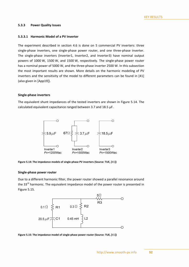
KEY RESULTS


5.3.3 Power Quality Issues

5.3.3.1 Harmonic Model of a PV Inverter

The experiment described in section 4.6 is done on 5 commercial PV inverters: three

single-phase inverters, one single-phase power router, and one three-phase inverter.

The single-phase inverters (Inverter1, Inverter2, and Inverter3) have nominal output

powers of 1000 W, 1500 W, and 1500 W, respectively. The single-phase power router

has a nominal power of 5000 W, and the three-phase inverter 2500 W. In this subsection

the most important results are shown. More details on the harmonic modeling of PV

inverters and the sensitivity of the model to different parameters can be found in [41]

(also given in [App19]).

Single-phase inverters

The equivalent shunt impedances of the tested inverters are shown in Figure 5.14. The

calculated equivalent capacitance ranged between 3.7 and 18.5 μF.

Figure 5.14: The impedance models of single-phase PV inverters (Source: TUE, [41])

Single-phase power router

Due to a different harmonic filter, the power router showed a parallel resonance around

the 33rd harmonic. The equivalent impedance model of the power router is presented in

Figure 5.15.

Figure 5.15: The impedance model of single-phase power router (Source: TUE, [41])


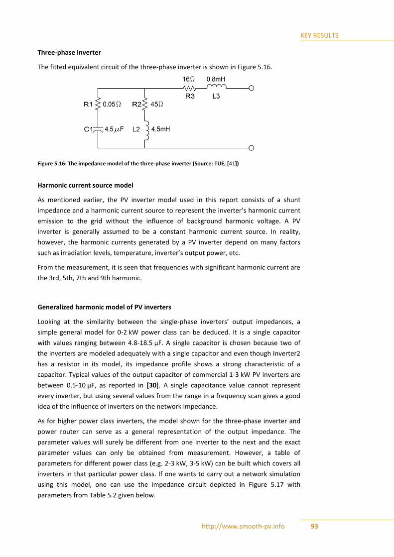
KEY RESULTS


Three-phase inverter

The fitted equivalent circuit of the three-phase inverter is shown in Figure 5.16.

Figure 5.16: The impedance model of the three-phase inverter (Source: TUE, [41])

Harmonic current source model

As mentioned earlier, the PV inverter model used in this report consists of a shunt

impedance and a harmonic current source to represent the inverter’s harmonic current

emission to the grid without the influence of background harmonic voltage. A PV

inverter is generally assumed to be a constant harmonic current source. In reality,

however, the harmonic currents generated by a PV inverter depend on many factors

such as irradiation levels, temperature, inverter’s output power, etc.

From the measurement, it is seen that frequencies with significant harmonic current are

the 3rd, 5th, 7th and 9th harmonic.

Generalized harmonic model of PV inverters

Looking at the similarity between the single-phase inverters’ output impedances, a

simple general model for 0-2 kW power class can be deduced. It is a single capacitor

with values ranging between 4.8-18.5 μF. A single capacitor is chosen because two of

the inverters are modeled adequately with a single capacitor and even though Inverter2

has a resistor in its model, its impedance profile shows a strong characteristic of a

capacitor. Typical values of the output capacitor of commercial 1-3 kW PV inverters are

between 0.5-10 μF, as reported in [30]. A single capacitance value cannot represent

every inverter, but using several values from the range in a frequency scan gives a good

idea of the influence of inverters on the network impedance.

As for higher power class inverters, the model shown for the three-phase inverter and

power router can serve as a general representation of the output impedance. The

parameter values will surely be different from one inverter to the next and the exact

parameter values can only be obtained from measurement. However, a table of

parameters for different power class (e.g. 2-3 kW, 3-5 kW) can be built which covers all

inverters in that particular power class. If one wants to carry out a network simulation

using this model, one can use the impedance circuit depicted in Figure 5.17 with

parameters from Table 5.2 given below.


KEY RESULTS


Figure 5.17: Simple model for single-phase inverters in the class 0-2 kW (left) and a more complex model for the class 2-5 kW (right) (Source: TUE, [41])

Table 5.2: Parameter values for general model of inverters in the class 2-5kW (Source: TUE, [41])

Nominal power

Parameter values

R1 C1 R2 L2 R3 L3

2-3kW 0.05 Ω 4.5 μF 45 Ω 4.5 mH 16 Ω 0.8 mH

4-5kW 0.1 Ω 20.5 μF 0.3 Ω 0.45 mH 5 Ω 0 mH

Values of harmonic current sources derived from the measurements are given in Table 5.3.

Table 5.3: Generalized values of harmonic current sources from the measured inverters (Source: TUE, [41])

Harmonic order

General 0-2kW model 2kW model from a literature [43]

General 2-5kW model

Absolute current at 0.9kW

Relative current to fundamental

Absolute current at 2kW


Absolute current at 2.5kW


3 0.04A 1.20% 0.25A 2.82% 0.16A 1.51%

5 0.03A 0.88% 0.25A 2.82% 0.08A 0.74%

7 0.02A 0.51% 0.12A 1.39% 0.03A 0.26%

9 0.02A 0.51% 0.11A 1.22% 0.02A 0.18%

Aggregation of PV inverters

The model from the previous subsection can be used for modeling a single PV inverter.

When multiple inverters are operating together, the sum of their harmonic currents is

lower than the arithmetic sum of their currents due to the phase angle diversity of

individual units. The value of the summed current is dependent on several factors: the

output powers of individual units (irradiance level, clouds, etc.), the connection


KEY RESULTS


impedance(s) of the units, and the background harmonic voltages originating from the

upstream network.

Due to these uncertainties and the time-varying nature of all of the elements, the

problem of harmonic aggregation is commonly addressed statistically. Instead of

determining the values of currents at a particular moment in time, the disturbance level

are evaluated as a probability level, e.g. the 95 % probability level which is the value not

exceeded for 95 % of the time. The approach suggested by [35], [44] aims at the 95 %

probability level, which is evaluated as:

√∑

(14)

where β is the summation coefficient of a particular order, ISUM is the aggregated

harmonic current, and Ii are individual harmonic currents. Values of the summation

coefficients of different orders are given in Table 5.4.

Table 5.4: Proposed values of the summation coefficient (Source: [35], [44])

Harmonic order β

h < 5 1

5 ≤ h ≤ 10 1.4

h > 10 2

Values of Table 5.4 can lead to both underestimation and overestimation of the

aggregated harmonic current at the connection point. In [45], it was shown by

laboratory and field measurement that these values mostly lead to underestimation of

harmonic currents.

To analyze the problem, we look at a field measurement conducted on a system of five

15 kVA inverters operating in parallel. The measurement was done using a multi-channel

measurement system with a time resolution of 1 s, and measurement duration of

approximately one week.


KEY RESULTS


1 2 3 4 5

x 105

0

1

2

3

4

Time [s]

Cu

rren

t [A

]

1 2 3 4 5

x 105

0

0.5

1

1.5

2

2.5

Time [s]C

urr

en

t [A

]

Figure 5.18: Variation of the summated 5th (left) and 7th (right) harmonic current during the measurement (Source: TUE)

The variation of the total 5th and 7th harmonic current (sum of five inverters) during the

measurement is shown in Fehler! Verweisquelle konnte nicht gefunden werden..

The PV panels of all five inverters are located close to each other. Due to this, they are

exposed to approximately the same irradiation levels during the day, and their loading

levels are very similar. Due to this, the effect of phase angle diversity is not pronounced.

A polar plot of the 5th harmonic current of individual inverters and the total current is

shown in Figure 5.19. Currents of individual inverters cover almost the same phase

angles, and due to this the total current is almost the arithmetical sum of the compo-

nents. In Figure 5.20 the calculated summation coefficients of this measurement are

shown. The values presented are mostly lower than suggested by technical standards.

This means that application of technical standards would lead to underestimation of

harmonic currents in this case. Values of the summation coefficient showed an increase

with the increase of the harmonic order, but much less than suggested in Table 5.4.

Values crossed 1.1 for all harmonic orders only after the 21st order.

Figure 5.19: Polar plot of the 5th harmonic current: individual inverters and the total current (Source: TUE)


KEY RESULTS


Figure 5.20: Summation coefficients calculated from the field measurement (Source: TUE)

Case study – influence of PV inverter impedances on LV network resonances

The system impedance is influenced by many elements. Knowing the exact composition

of loads, both in the low voltage network and upstream networks, is usually difficult and

also changing in time. Network reconfigurations also add to the time varying nature of

the impedance, so each calculation can serve only for a particular moment in time. For

this reason it is usual to calculate the polar diagram of the impedance for all predicted

topology and load changes.

The adopted test network is a household low voltage network with a large amount of PV

inverters connected. This network was chosen because the capacitance of PV inverters

shifts the first parallel resonance in the low frequency range [46].

Cables were modeled with their PI equivalents. Skin effect was not taken into account.

Both the LV and the medium voltage (MV) networks are cable networks.

Transformers were modeled as series RL circuits. Their capacitances were not taken into

account as the maximal frequency of interest was 3 kHz.

Power factor correction (PFC) units were modeled only as a capacitance without losses.

Household loads were modeled as parallel RC circuits and parallel RLC circuits (several

scenarios). The capacitance should represent the input capacitance of all power

electronic devices, mainly their input filters. A value of 0.6 µF per house is adopted here.

Induction motors were modeled as their locked rotor inductance. The total adopted

power of linear loads in the houses was 500 W, and induction motors were accounted

for as (0 – 30) % of this load, in several steps. Resistance should represent the linear

3 5 7 9 11 13 15 17 19 21 23 25 27 29 311

1.05

1.1

1.15

1.2

1.25

1.3

Harmonic order

Su

mm

atio

n c

oe

ffic

ien

t


KEY RESULTS


loads without motors. Depending on the number of induction motors, resistance was

changed to get the same total power of linear loads.

Photovoltaic inverters were modeled as their input capacitance. Since the value of

inverter capacitance is not known, it was varied in the range (0.5 – 10) µF. The total

installed power of PV inverters in the low voltage network is 300 kW, mostly composed

of 2 kW units, while the peak load of all loads together is approximately 150 kVA. By

analyzing the network’s harmonic impedance for several values of the inverters’ output

capacitance we can determine the range in which the first parallel resonance should be

located. Finding the exact value is a difficult task because some of the parameters are

approximate, but a range of values will usually indicate if a problem is to be expected.

The effect of lumping loads was examined in three steps. In the first step, all loads were

connected directly at the low voltage busbar. In the second step, feeders were

separated in the low voltage network, with lumped loads on feeders and feeder

branches. In the last step, all houses and inverters were modeled separately.

The medium voltage network was modeled in two ways. The simple version of the

model is a series RL circuit, representing the short-circuit power of the network and the

R to X ratio. A more detailed model was also used, representing all MV feeders until the

HV/MV substation, and one 1.4 MW CHP (combined heat and power) generator in the

MV network and several configurations of PFC in the MV network. The HV network was

represented with its short-circuit level.

A schematic diagram of the low voltage part of the example network is shown in Figure

5.21. The medium voltage part of the network is presented in Figure 5.22. The low

voltage network is connected to busbar 13 of the MV network.

All four feeders are numbered in the LV network, while in the MV network only four

busbars are numbered (2, 9, 12, and 13), since changes of elements were applied only

on these busbars.

Figure 5.21: Low voltage part of the analyzed network (Source: [47])


KEY RESULTS


Figure 5.22: Medium voltage part of the analyzed network (Source: [47])

5.3.3.2 Effect of lumping loads

The number of loads in a LV network is usually too large to allow for modeling each load

separately. For this reason, loads are commonly lumped into equivalent loads with some

feeders and load parameters neglected. This leads to uncertainty of the outcome.

To illustrate the effect of lumping loads, we compare the harmonic impedance versus

frequency at the low voltage busbar of the example network for three cases. In the first

case we look at the whole low voltage network as a single parallel RLC load connected

directly at the transformer (case: all lumped). In the second step, we lump the separate

feeders as shown in Figure 5.23, with feeders and feeder branches lumped as parallel

RLC loads after cables (case: lumped feeders). In the third step, we uncouple the loads

to more branches, with short feeders divided in five sections, and longer feeders in 10

sections (case: no lumping).

The solution of the “most realistic” case (no lumping) falls between the two other cases.

In comparison with the case with everything lumped at the busbar, lumping complete

feeders will add extra inductance in the circuit, resulting in a lower resonant frequency

(in this case by almost 30 Hz). In the case where nothing is lumped, most capacitances

are connected via a lower inductance, resulting in a smaller frequency change from the

first case (less than 20 Hz).


KEY RESULTS


Figure 5.23: Effect of lumping loads on the example LV network (Source: [47])

In conclusion, lumping all loads leads to an increase of the resonant frequency, but with

acceptable errors if feeder lengths are short. It does not reveal all resonances in the

system. Lumping separate feeders leads to a decrease in the resonant frequency, with

smaller errors. It also reveals additional resonances but the uncertainty is larger at

higher frequencies.

To avoid high model complexity, in the following subsections the model with lumped

feeders is used for analyzing other effects.

5.3.3.3 Effect of inverters’ output capacitance

To analyze the effect of capacitive loads on the frequency of the first parallel resonance,

we look at the simplified expression:

( ) ⁄ (15)

where Z is the equivalent network impedance, L is the inductance of the upstream

network, and C is the capacitance of loads connected to the busbar. Capacitances

change the resonant frequency directly: a ∆C change of capacitance changes the

resonant frequency by 1/√∆C.

In the example network there are no power factor correction units in the low voltage

network; the capacitances are mostly located in input filters of PV inverters. If the values

of these capacitances are not known, this leads to a large range of possible solutions.

Figure 5.24 shows the impedance characteristic for four capacitance assumptions.

Initially, 8 µF is assumed for each 2 kW inverter; then a ± 20 % capacitance uncertainty is

taken into account; in the end, it was assumed that 2 µF is the input capacitance of each

2 kW inverter.

0 500 1000 1500 2000 2500 30000

0.2

0.4

0.6

0.8

1

1.2

1.4

1.6

f [Hz]

Z [O

hm

]

all lumped

lumped feeders

nothing lumped


KEY RESULTS


Figure 5.24: The effect of inverter capacitance on the impedance of the example network (Source: [47]])

If the capacitance is not known initially, the difference between assuming 2 and 8 µF per

inverter in this case leads to a 500 Hz difference in the resonant frequency. If the

capacitance is known, and the uncertainty is taken into account as ±20 %, differences of

60 Hz can be noticed.

More results of the investigation about network impedances can be found in [47] (also

given in [App20]).

5.3.4 Voltage Dip Studies

This subsection presents a summary of the main results of voltage-dip simulations with a

high share of PV inverters present in the network, based on the methodology presented

in chapter 4.7. The detailed results of these simulations can be found in [42] (also found

in [App18]).

5.3.4.1 Single-phase voltage dips

The voltage and current waveforms during a single-phase dip with a remaining voltage

of 0.7 p.u. are shown in Figure 5.25.

0 500 1000 1500 2000 2500 30000

0.2

0.4

0.6

0.8

1

1.2

1.4

f [Hz]

Z [O

hm

]

8 uF/inv.

8 uF -20%

8 uF +20%

2 uF/inv.


KEY RESULTS


Figure 5.25: Voltage at the PCC and current of the first inverter during a single-phase voltage dip down to 0.7 p.u. (Source: [42])

The available voltage support provided by the inverters for different remaining voltages

with single-phase voltage dips are given in Table 5.5.

Table 5.5 Available voltage support during single-phase voltage dips (Source: [42])

Remaining voltage [p.u.]

rms value of voltage at PCC with (without) Inverters Connected [V]

Voltage increase due to inverters [V]

Phase A Phase B Phase C Phase A Phase B Phase C

0.3 161.3(146.0) 228.9(214.4) 161.3(146.0) 15.3 14.5 15.3

0.4 170.2(154.6) 228.9(214.4) 170.2(154.6) 15.6 14.5 15.6

0.5 179.5(163.7) 228.9(214.4) 179.5(163.7) 15.8 14.5 15.8

0.6 188.9(173.3) 228.9(214.4) 188.9(173.3) 15.6 14.5 15.6

0.7 198.6(183.2) 228.9(214.4) 198.6(183.2) 15.4 14.5 15.4

0.8 208.5(193.3) 228.9(214.4) 208.5(193.3) 15.2 14.5 15.2

0.9 218.6(203.8) 228.9(214.4) 218.6(203.8) 14.8 14.5 14.8


KEY RESULTS


5.3.4.2 Two-phase voltage dips


under two-phase voltage dips are given in Table 5.6.

Table 5.6 Available voltage support during two-phase voltage dips (Source: [42])

Dip depth in one phase (pu)

rms value of voltage at PCC with (without) Inverters Connected / V

Increase Value / V

Phase A Phase B Phase C Phase A Phase B Phase C

0.5 118.5(107.2) 179.5(163.7) 179.5(163.7) 11.3

0.6 144.0(128.6) 188.9(173.3) 188.9(173.3) 15.4

0.7 166.0(150.1) 198.6(183.2) 198.6(183.2) 15.9 15.8 15.8

0.8 187.3(171.5) 208.5(193.3) 208.5(193.3) 15.8 15.6 15.6

0.9 208.1(192.3) 218.6(203.8) 218.6(203.8) 15.8 15.4 15.4

5.3.4.3 Three-phase dips


under three-phase voltage dips are given in Table 5.7.

Table 5.7 Available voltage support during three-phase voltage dips (Source: [42])

Dip depth in two phases (pu)

rms value of PCC with inverters connected / V

Voltage at PCC without inverters / V

Increase / V

0.5 118.4 107.2 11.2

0.6 144 128.6 15.4

0.7 166.1 150.1 16

0.8 187.2 171.5 15.7

0.9 208.1 192.3 15.8

1.0 228.9 214.4 14.5


KEY RESULTS


5.3.4.4 Summary of Short-Circuit (Voltage Dip) Simulations

Dynamic simulations on the example LV network showed very limited voltage support

provided by the PV inverters, between 10 and 15 V in all situations simulated. These

numbers cannot be taken as general because different network impedance and powers

of inverters would lead to a different range of values.

The main reason for the low influence is the current limitation of inverters. If the

inverters had a current limit higher than 120 % of the nominal current, they would be

capable of providing more voltage support. An optimal value for the current limit needs

to take into account the hardware restrictions of inverters and the global impact on

voltage levels during network faults. This question should be explored further in the

future.

Measured voltage-dip sensitivity of inverters

One of the safety requirements of PV inverters concerns the anti-islanding protection

which ensures that the inverters stop feeding power when the grid properties are not

within the given range. For example, in IEEE Std 929-2000, PV inverters are

recommended to stop energizing the network whenever the voltage at PoC is not within

88 % and 110 % of its nominal voltage. This requirement varies from one country or

standard to the other. German standard DIN/VDE 0126 requires inverters to disconnect

from the grid within 0.2 s when the voltage is not within 80 % and 115 % of its nominal

voltage. In the future it can be expected that inverters will have to include ride-through

capability if they gain a significant share in production.

The inverters used for harmonic modeling were tested for their sensitivity to voltage

dips. Results of these measurements are summarized in Figure 5.26. The differences in

disconnection time between one inverter and another are determined by many factors.

The first factor is the resolution of the inverter’s measurement of the voltage level at

PoC, i.e. how often and for how long the inverter measures the voltage level. The second

factor is the amount of information needed by each inverter to decide whether a

situation is a disturbance and it needs to disconnect. One inverter might decide to

disconnect after a first reading, while others need more readings to be “sure” that a

situation is indeed a disturbance. Lastly, each inverter needs a different amount of time

from deciding to disconnect to actually disconnecting from the grid. This factor is

determined by the speed of the microcontrollers inside the inverter.


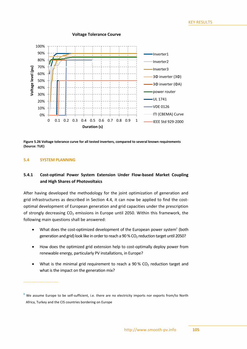
KEY RESULTS


Figure 5.26 Voltage tolerance curve for all tested inverters, compared to several known requirements (Source: TUE)

5.4 SYSTEM PLANNING

5.4.1 Cost-optimal Power System Extension Under Flow-based Market Coupling

and High Shares of Photovoltaics

After having developed the methodology for the joint optimization of generation and

grid infrastructures as described in Section 4.4, it can now be applied to find the cost-

optimal development of European generation and grid capacities under the prescription

of strongly decreasing CO2 emissions in Europe until 2050. Within this framework, the

following main questions shall be answered:

What does the cost-optimized development of the European power system6 (both

generation and grid) look like in order to reach a 90 % CO2 reduction target until 2050?

How does the optimized grid extension help to cost-optimally deploy power from

renewable energy, particularly PV installations, in Europe?

What is the minimal grid requirement to reach a 90 % CO2 reduction target and

what is the impact on the generation mix?

..............................

6 We assume Europe to be self-sufficient, i.e. there are no electricity imports nor exports from/to North

Africa, Turkey and the CIS countries bordering on Europe

0%

10%

20%

30%

40%

50%

60%

70%

80%

90%

100%

0 0.1 0.2 0.3 0.4 0.5 0.6 0.7 0.8 0.9 1

Vo

ltag

e le

vel (

pu

)

Duration (s)

Voltage tolerance curve

Inverter1

Inverter2

Inverter3

3Φ inverter (3Φ)

3Φ inverter (ΦA)

power router

UL 1741

VDE 0126

ITI (CBEMA) Curve

IEEE Std 929-2000

Voltage Tolerance Courve


KEY RESULTS


5.4.1.1 Scenario definition

The modeling framework is used to simulate two scenarios that both achieve a 90 %

CO2-target in 2050 (compared to 1990 levels) but differ with respect to the actual

extension of the transmission grid in the system. Scenario 1 is characterized by cost-

optimized grid extensions, whereas Scenario 2 determines the cost-optimal develop-

ment of the European power system if grid extensions are avoided as much as possible

while still reaching ambitious CO2 targets (i.e. a 90 % reduction by 2050). Scenario 2 thus

examines what might happen if hardly any extension to the power grid is possible, for

example, due to long permission procedures or low social acceptance.

The main assumptions of the two scenarios are listed in Table 5.8. As can be seen, the

only difference is made with respect to the way the grid is expanded between 2020 and

2050. Hence, by comparing the two scenarios, the specific effect of grid extensions can

be isolated and analyzed.

Table 5.8: Main scenario assumptions (Source: UoC, Energynautics)

Scenario 1 Scenario 2

Nuclear power Limited to planned projects

European CO2 reduction quota 90% in 2050 (compared to 1990 levels)

Grid expansion until 2020 Limited to planned projects (TYNDP)

Grid expansion until 2050 Optimal Minimal

5.4.1.2 Iteration Results

According to the procedure illustrated in Figure 4.4, the two models are run sequentially

in an iterative process in order to jointly optimize generation and grid infrastructures as

well as their operation. In the market model, PTDF matrices are updated before starting

a new run in order to include PTDF matrices that are consistent with the previously

determined optimized line capacities and their corresponding impedances. These PTDF

matrices are determined by Energynautics based on the AC load flow calculations in the

European transmission grid model.

On running the optimization, it was found that the grid extensions in Scenario 2 were so

small that no iteration of the PTDFs was necessary. For Scenario 1 there were significant

changes and therefore iterations were run until convergence was reached. The

convergence is analyzed with respect to the difference in the accumulated (2011-2050)

discounted total system costs (see chapter 4.3.1 for a definition) between iteration i and

i+1. The development of the total system costs during the iteration in Scenario 1 is


KEY RESULTS


depicted in Figure 5.27. As can be observed, the difference in total system costs

between iteration reduces to less than 0.02 % (or 0.5 Bn. €) after iteration 4.

Consequently, the iteration is stopped after step 5.

Figure 5.27: Development of total system costs during the iteration (Source: UoC)

Figure 5.28 shows the corresponding development of the optimal line capacity for four

example lines during the iterative process. As can be seen, optimal line capacities

converge after iteration 4.

Figure 5.28: Development of optimal line capacities for four example lines during the iteration (Source: UoC)

2816

2820

2824

2828

2832

2836

1 2 3 4 5

Syst

em

co

sts

[Bn

. €]

Iteration step

0

1000

2000

3000

4000

5000

6000

7000

1 2 3 4 5

Op

tim

al li

ne

cap

acit

y [M

W]

Iteration step

RS1

EE-LV1

NL3

AT-DE1


KEY RESULTS


Results Scenario 1: Optimal grid extension

The results of Scenario 1 (cost-optimized power generation and transmission grid

extension) are taken from the last iteration step. The results for the installed generation

capacities and their gross electricity generation volumes are presented in Figure 5.29.

Figure 5.29: Installed generation capacities and gross electricity generation in Europe in Scenario 1 (Source: UoC)

It can be seen that an increasing level of demand is covered by a substantially changing

mix of generation technologies.7 The shift from conventional generation, mainly nuclear,

lignite, coal and gas to an increasingly renewable based electricity generation is mainly

driven by ambitious CO2 reduction targets (the CO2 quota reduction quota reaches 90 %

in 2050). Moreover, the expansion of nuclear power is restricted to currently planned

projects and therefore plays a minor role in Europe’s future generation mix.

..............................

7 Electricity demand is an exogenous model input, based on assumptions regarding the specific economic

development of the various nations covered in the analysis.

0

500

1000

1500

2000

2500

3000

2011 2020 2030 2050

inst

alle

d c

apac

itiy

[G

W]

0

1000

2000

3000

4000

5000

6000

2011 2020 2030 2050

elec

tric

ity

gen

erat

ion

[TW

h]

Nuclear Lignite Coal Gas Oil

Others Water Wind Sun Biosolid

Biogas Storage Geothermal


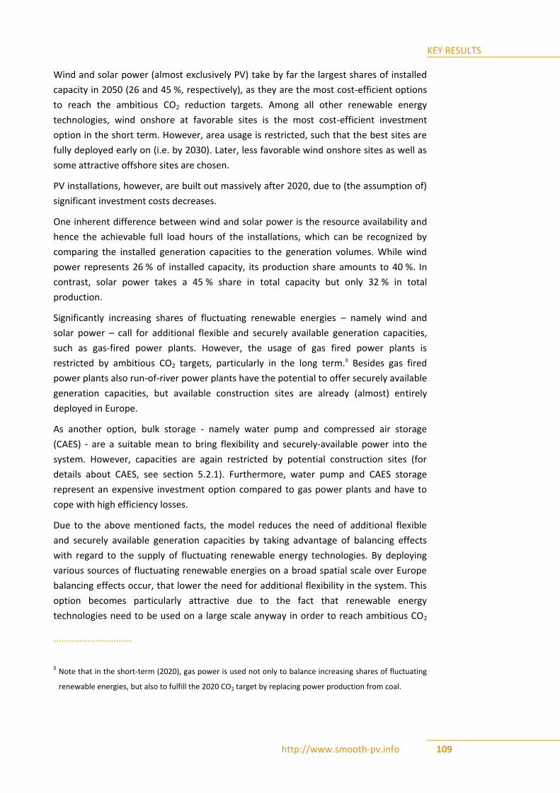
KEY RESULTS


Wind and solar power (almost exclusively PV) take by far the largest shares of installed

capacity in 2050 (26 and 45 %, respectively), as they are the most cost-efficient options

to reach the ambitious CO2 reduction targets. Among all other renewable energy

technologies, wind onshore at favorable sites is the most cost-efficient investment

option in the short term. However, area usage is restricted, such that the best sites are

fully deployed early on (i.e. by 2030). Later, less favorable wind onshore sites as well as

some attractive offshore sites are chosen.

PV installations, however, are built out massively after 2020, due to (the assumption of)

significant investment costs decreases.

One inherent difference between wind and solar power is the resource availability and

hence the achievable full load hours of the installations, which can be recognized by

comparing the installed generation capacities to the generation volumes. While wind

power represents 26 % of installed capacity, its production share amounts to 40 %. In

contrast, solar power takes a 45 % share in total capacity but only 32 % in total

production.

Significantly increasing shares of fluctuating renewable energies – namely wind and

solar power – call for additional flexible and securely available generation capacities,

such as gas-fired power plants. However, the usage of gas fired power plants is

restricted by ambitious CO2 targets, particularly in the long term.8 Besides gas fired

power plants also run-of-river power plants have the potential to offer securely available

generation capacities, but available construction sites are already (almost) entirely

deployed in Europe.

As another option, bulk storage - namely water pump and compressed air storage

(CAES) - are a suitable mean to bring flexibility and securely-available power into the

system. However, capacities are again restricted by potential construction sites (for

details about CAES, see section 5.2.1). Furthermore, water pump and CAES storage

represent an expensive investment option compared to gas power plants and have to

cope with high efficiency losses.

Due to the above mentioned facts, the model reduces the need of additional flexible

and securely available generation capacities by taking advantage of balancing effects

with regard to the supply of fluctuating renewable energy technologies. By deploying

various sources of fluctuating renewable energies on a broad spatial scale over Europe

balancing effects occur, that lower the need for additional flexibility in the system. This

option becomes particularly attractive due to the fact that renewable energy

technologies need to be used on a large scale anyway in order to reach ambitious CO2

..............................

8 Note that in the short-term (2020), gas power is used not only to balance increasing shares of fluctuating

renewable energies, but also to fulfill the 2020 CO2 target by replacing power production from coal.


KEY RESULTS


targets. However, balancing effects of fluctuating renewable energy supply across

Europe can only be realized by building additional transmission grid capacities.

The results of the cost-optimal power system development with respect to the power

transmission grid are shown in Table 5.9.

Table 5.9: AC and DC grid extensions in Scenario 1 (Source: UoC, Energynautics)

Scenario 1

AC Grid [GVA] DC Grid [GW]

Installed capacity 2011 967.9 9.3

Capacity added 2011-2020 82.8 14.9

Capacity added 2020-2030 331.0 30.2

Capacity added 2030-2050 611.8 181.1


Starting from an initial capacity of 967.9 GVA AC and 9.3 GW DC grid in 2011, both

technologies are massively extended until 2050 and reach levels of 1993.5 GVA (AC) and

235.5 GW (DC), respectively. As such, the AC grid capacity is more than doubled. The

most substantial extensions occur during the last two decades considered in the

simulation, between 2030 and 2050. This is due to two reasons: first, a steadily

increasing demand has to be covered. Second, the CO2 quota becomes more restrictive

over time and thus calls for additional renewable generation capacities that have to be

connected to load centers. As reported in Table 5.9, DC capacity extensions amount to

226.2 GW between 2011 and 2050, thus reaching a capacity of 235.5 GW in 2050.

The distribution of AC and DC capacities in Europe is shown in Figure 5.30. As can be

seen, the overlay DC grid is mainly used to transport power from (remote) renewable

production sites to load centers, e.g.:

Wind power from the northern coasts of Great Britain to London, and further

towards the continent (i.e. France, Belgium and the Netherlands).

Wind power from Northern Germany, Northern Poland and the Baltic towards load

centers in Central Europe.

Solar power from Southern Spain to Madrid and further towards France.

Solar power from Southern Italy to Milano and further towards Central Europe.


KEY RESULTS


Figure 5.30: Grid upgrades between 2020 and 2050 (left hand side) and grid capacities in 2050 (right hand side) (Source: Energynautics)

As can be observed in the results, DC becomes an attractive option to the optimization

algorithm, especially for long distance power transmission. This is thanks to several

reasons:

Since it can provide point-to-point transfers, DC lines avoid the need to build out

the AC network to accommodate the parallel loop flows caused by big power

transfers over long distances. In many cases, this advantage makes DC a cheaper

option than AC.

For long distances, the DC lines are both cheaper per MW of active power

transferred per km and also take more direct routes than the existing AC power

corridors (resulting in fewer kilometers that need to be upgraded). This must be

weighed against the additional converter costs that DC lines bring.

A limit of 15 GVA was set for each of the aggregated AC transmission lines in the

model, to represent the maximum amount that can be feasibly built and

transported in a single AC power corridor.

Results Scenario 2: Minimal grid extension

In contrast to Scenario 1 in which the transmission grid is heavily extended, Scenario 2

sheds light on the cost-optimal development of the European power system if grid

extensions are avoided as much as possible while still reaching ambitious CO2 targets

(i.e. a 90 % reduction in 2050). Scenario 2 thus deals with the issue of hardly being able


KEY RESULTS


to extend the power grid, e.g. due to long permission procedures or low social

acceptance.

Technically, in Scenario 2 the model is modified so that the grid extension costs are

assumed to be prohibitively high. The optimization algorithm is thus forced to search for

the cost-optimal solution comprising as few grid extensions as possible.

The results of Scenario 2 have to been seen in the context of the modeling approach

that was previously described. Specifically, the model is forced to allocate generation

capacities to the single nodes within a market region according to an exogenous

allocation key. The model is thus not able to optimally choose the location of the

generation capacities within the market regions. As a consequence, (prohibitively

expensive) line capacities might be needed because generation capacities cannot be

sited alternatively within the market region in the model.9

Modeling a nodal pricing regime where each node of the transmission grid is its own

market region would help to overcome the drawback of using exogenous allocation keys

to allocate generation capacities to the single nodes within the market regions.

However, this would further enlarge the optimization problem and could not be solved

in a reasonable time.

As can be seen in Figure 5.31, the capacity and generation mixes are highly affected by

this alteration. The same increasing level of electricity demand as in Scenario 1 has to be

covered by increasing shares of renewable energy technologies (due to the CO2 quota).

However, two effects arise due to the avoidance of grid extensions:

Renewable energy technologies cannot be deployed at sites where resource

availability is best. As a consequence, wind and solar power generation

technologies have significantly lower utilization rates (i.e. full load hours). More

capacity is thus needed to cover the demand, resulting in additional investment

costs.

Alternative renewable energy sources are deployed as wind and solar power area

potentials close to load centers are exhausted. Only limited areas are available for

wind and solar power production close to load centers. In order to avoid grid

expansions, alternative (renewable energy) technologies are deployed that can be

built close to load centers, particularly biomass and geothermal power. As biomass

and geothermal power are comparatively flexible and securely available, lower

storage capacities are needed in Scenario 2.

..............................

9 In contrast, the distribution of capacities between market regions across Europe is optimally chosen as

these represent separate decision variables in the model.


KEY RESULTS


Figure 5.31: Installed generation capacities and gross electricity generation in Europe in Scenario 2 (Source: UoC)

The development of grid capacities in Scenario 2 is reported in Table 5.10. As expected,

very little additional transmission grid capacity is built, amounting to an additional

capacity of 89.0 GVA AC (increase of 9 %) and 14.9 GW DC (increase of 160 %).10

Table 5.10: AC and DC grid extensions in Scenario 2 (Source: UoC, Energynautics)

Scenario 2

AC Grid [GVA] DC Grid [GW]


Capacity added 2011-2020 82.8 14.9

Capacity added 2020-2030 0 0.0

Capacity added 2030-2050 6.2 0.0


Comparison of Scenario 1 and 2

..............................

10 Note that the line capacities for 2020 are not optimized as we argue that for the year 2020 optimized grid

extensions would not be realistic within this timeframe, due to long planning and permission procedures of

such projects. Capacities for 2020 are based on mid-term projects in the TYNDP.

0

500

1000

1500

2000

2500

3000

2011 2020 2030 2050

inst

alle

d c

apac

itiy

[G

W]

0

1000

2000

3000

4000

5000

6000

2011 2020 2030 2050elec

tric

ity

gen

erat

ion

[TW

h]

Nuclear Lignite Coal Gas OilOthers Water Wind Sun BiosolidBiogas Storage Geothermal


KEY RESULTS


The difference in total grid extensions until 2050 in Scenario 1 and Scenario 2 is

substantial. Whereas capacity additions amount to 1025 GVA (AC) in Scenario 1 (optimal

grid extension), capacity additions sum up to 89 GW (AC) in Scenario 2 (minimal grid

extension).

The system value of grid extensions for the power system is reflected in the difference

between total system costs in the two scenarios that are reported in Table 5.11. Total

system costs are accumulated (2011-2050) and discounted (at a rate of 5 %) and include

investment costs, fixed operation and maintenance costs, variable production costs and

costs due to ramping thermal power plants. While accumulated discounted total system

costs until 2050 amount to 2833 bn. € in Scenario 1, they amount to over 3424 bn. € in

Scenario 2. The significant difference of 591 bn. € (20.9%) clearly demonstrates that

significant extensions help to cost-efficiently deploy renewable power sources in

Europe.11

Table 5.11: Comparison of total system costs in Scenario 1 and 2 (Source: UoC, Energynautics)


Total system costs [bn. €] 2833 3424

Cost difference [bn. €] 591 (20.9%)

Concerning PV’s share in the load coverage in 2050, it adds up to 1680 TWh (32%) with

the optimal grid extension, while with the minimum grid extension it is reduced to

1176 TWh (23 %)12. In contrast to Scenario 1, in which regions with higher annual solar

irradiation (such as Southern Spain or Southern Italy) could be exploited well due to the

necessary grid in place, many solar installations in Scenario 2 without the ample grid

extension moved further to the North, thus reducing the amount of annual full load

hours of PV in Europe.

Regarding the transmission network loading, a useful measure is to add up for each line

the power flowing through it at a given time multiplied by the line’s length (measured in

units of MWkm). This gives an indication of how much power is being transported over

long distances in the model. As can been seen from Figure 5.32 there is a substantial

..............................

11 For the simulation of Scenario 2, grid extension costs were assumed to be prohibitively high. However, for

the calculation of the total system costs in Scenario 2 as they are reported in Table 4.6, the same

(standard) grid extensions costs were assumed as in Scenario 1.

12 In scenario 1 CSP has a negligible share compared to PV in terms of produced energy. In scenario 2 the

ratio PV:CSP is higher at 70:1.


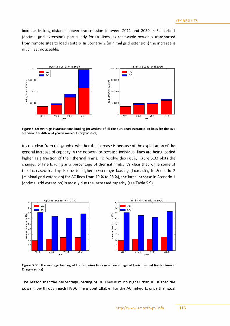
KEY RESULTS


increase in long-distance power transmission between 2011 and 2050 in Scenario 1

(optimal grid extension), particularly for DC lines, as renewable power is transported

from remote sites to load centers. In Scenario 2 (minimal grid extension) the increase is

much less noticeable.

Figure 5.32: Average instantaneous loading (in GWkm) of all the European transmission lines for the two scenarios for different years (Source: Energynautics)

It’s not clear from this graphic whether the increase is because of the exploitation of the

general increase of capacity in the network or because individual lines are being loaded

higher as a fraction of their thermal limits. To resolve this issue, Figure 5.33 plots the

changes of line loading as a percentage of thermal limits. It’s clear that while some of

the increased loading is due to higher percentage loading (increasing in Scenario 2

(minimal grid extension) for AC lines from 19 % to 25 %), the large increase in Scenario 1

(optimal grid extension) is mostly due the increased capacity (see Table 5.9).

Figure 5.33: The average loading of transmission lines as a percentage of their thermal limits (Source: Energynautics)

The reason that the percentage loading of DC lines is much higher than AC is that the

power flow through each HVDC line is controllable. For the AC network, once the nodal


KEY RESULTS


power balances are fixed, the pattern of power flow is determined by the impedances of

the network. This can lead to parallel loop flows in the AC network, whereby power does

not necessarily take the shortest route through the network, but spreads out among

multiple parallel routes, burdening wide areas of the network. Loop flows already cause

problems in Europe today, e.g. with internal power transactions in Germany burdening

the networks of Poland, the Czech Republic and the Benelux countries. The HVDC lines

in the model were placed and dimensioned to avoid these parallel loop flows in the AC

network, making them a tool of Flexible AC Transmission Systems (FACTS). In reality,

other FACTS tools would also be available to network operators to steer AC power flows,

such as phase-shifting transformers. However, these were not considered in the study.

Focusing on Scenario 1 in the year 2050, it is also interesting to understand which

generation technology is causing the long-distance power flows in the model. The

correlation of solar generation to loading (measured in MWkm again) is very weak, with

a Pearson correlation coefficient of r = 0.02, whereas for wind (both on- and offshore) it

is a much more significant r = 0.84 (r = 0 is no correlation and r = 1 would be perfect

correlation). This correlation is shown in Figure 5.34 for the typical days (refer to section

4.3.3) of the simulation. This agrees with the general expectation that wind benefits

more from grid extensions than solar does.

Figure 5.34: Correlation of wind generation and line loading (measured in MWkm) in the European system over the snapshots used for the optimization for 2050 in Scenario 1 (Source: Energynautics)

PV Penetration per country in Scenario 1

The PV installed capacities for the year 2050 in Scenario 1 (optimal grid extension) are

plotted for the individual countries in Figure 5.35. Significant capacity is seen in many

countries, including northerly ones, exhausting the surface area potentials in many

cases. This large expansion of PV is facilitated by big assumed reductions in installation

costs by 2050.


KEY RESULTS


Figure 5.35: Total installed capacity of photovoltaics per country for year 2050 in Scenario 1 (Source: Energynautics)

In some countries, strikingly in Hungary, Lithuania, Latvia and Romania, the capacities

are quite high relative to the demand in the country, due to large available surface areas

compared to population. This is seen in Figure 5.36, which plots the fraction of total

demand over the year for 2050 covered by photovoltaic generation.

Figure 5.36: Share of photovoltaics in covering each country's yearly demand in year 2050 for Scenario 1 (Source: Energynautics)

In many countries the instantaneous penetration of PV (as a fraction of the instan-

taneous demand) reaches well over 100 %, as shown in Figure 5.37. Along with full-

scale-converter-coupled wind power plants, this high fraction of non-synchronous

generation will present challenges for frequency control.


KEY RESULTS


Figure 5.37: Maximum instantaneous penetration of PV as a fraction of each county's demand for the year 2050 in Scenario 1 (Source: Energynautics)

5.4.2 Results of Extreme Event Tests

After the long-term optimization of the generation and transmission systems presented

in the previous section, the resulting grid infrastructure was also tested against a 10-

day-long extreme event of low wind and low sun (see Section 4.4.3 for the full

description). This was done separately for the two scenarios in 2030 and 2050, under

the assumption that storage devices at the start of the event were half full and that no

line became overloaded beyond its thermal limit, taking account of an n-1 security factor

of 70 % and assuming a power factor of 95 % when doing DC load flow.

5.4.2.1 Results for Scenario 1: Optimal Grid Extension

The generation and grid assets were able to supply all load during the extreme event

with the optimal grid extension, in both 2030 and 2050. The storage and controllable

generation assets (fossils, biofuels and remaining nuclear plants) were able to

coordinate to prevent outages.

In fact in 2050 it was possible to optimize the dispatch with respect to line loading

during the extreme event to ensure that no transmission line in the system was loaded

over more than 47 %. The dispatch in Germany is presented in Figure 5.38 as an

example.


KEY RESULTS


Figure 5.38: Power dispatched to meet demand in Germany during the extreme event for Scenario 1; where generation goes above demand, power is being stored and/or exported (source: Energynautics)

It can be seen here that the controllable generation is run at full capacity for most of the

first week, before growing wind availability begins to displace it. For Germany, AC

imports from the rest of the network are extremely important during this timeframe,

covering up to a quarter of the load. Storage also plays an important part, mainly in

order to cover evening peak loads when there is no PV generation.

To see how critical storage is during the extreme event, the “state of charge” as a

fraction of maximum storage capacity in each synchronous zone is plotted in Figure

5.39.

Figure 5.39: Fraction of available storage capacity used during the extreme event in Scenario 1 (Source: Energynautics)

It can be seen how the storage is initially charged at the start of the week, in anticipation

of the coming bottleneck, and then run down towards the end of the week, until almost

all storage is empty. During the final four days, during which wind availability is greater,

the storage can be recharged.

Ireland here presents an interesting case, because storage was critically important to

ensuring its load was covered during the event. It has a peak load in 2050 of 5.5 GW, a

high dependence on renewables (mainly onshore wind power) and only a 3 GW DC link

with Great Britain to import electricity from elsewhere. This explains why the storage in

Ireland is charged so high at the start of the event, to ensure load is covered in the

following days.


KEY RESULTS


5.4.2.2 Results for Scenario 2: Minimal Grid Extension

For the minimal grid extension case 2030 was unproblematic, but in 2050 there were

minor issues with line loading. In 2050 there was enough power in the system to cover

all loads, but it was not possible to achieve the necessary loading of each line of 66.5 %

(assuming an n-1 security factor). The model was optimized to determine the minimum

additional grid extension needed to reach this loading limit during the extreme event,

and it was found that only three lines needed to be extended: two in NORDEL and one in

Greece. The total necessary extension, assuming it could be done in small continuous

steps instead of a single 1500 MVA pieces, was 950 MVA in total for the three lines,

which does not represent a significant extension. As such, it can be concluded that the

simplifications made for the algorithm developed to jointly optimize generation and grid

infrastructures in a cost-efficient way represent a feasible approach, even when long-

lasting extreme events are not explicitly covered in the market model.

Compared to Scenario 1, the network and generation fleet are different in Scenario 2,

and these differences are reflected in the sample dispatch for Germany in Figure 5.40.

Figure 5.40: Power dispatched to meet demand in Germany during the extreme event in Scenario 2 (Source: Energynautics)

Here there is a much bigger contribution from controllable resources, given the large

geothermal capacity built out by the optimization due to strict avoidance of grid

extensions. We see also bigger displacement of controllable generation by wind, solar

and storage during the event, which is also necessitating steep ramp rates from the

controllable fleet. Since the network is much weaker, AC imports play a much smaller

role in covering Germany’s load.

The state of charge for the event in the various synchronous zones is shown below.


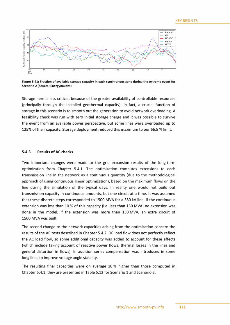
KEY RESULTS


Figure 5.41: Fraction of available storage capacity in each synchronous zone during the extreme event for Scenario 2 (Source: Energynautics)

Storage here is less critical, because of the greater availability of controllable resources

(principally through the installed geothermal capacity). In fact, a crucial function of

storage in this scenario is to smooth out the generation to avoid network overloading. A

feasibility check was run with zero initial storage charge and it was possible to survive

the event from an available power perspective, but some lines were overloaded up to

125% of their capacity. Storage deployment reduced this maximum to our 66.5 % limit.

5.4.3 Results of AC checks

Two important changes were made to the grid expansion results of the long-term

optimization from Chapter 5.4.1. The optimization computes extensions to each

transmission line in the network as a continuous quantity (due to the methodological

approach of using continuous linear optimization), based on the maximum flows on the

line during the simulation of the typical days. In reality one would not build out

transmission capacity in continuous amounts, but one circuit at a time. It was assumed

that these discrete steps corresponded to 1500 MVA for a 380 kV line. If the continuous

extension was less than 10 % of this capacity (i.e. less than 150 MVA) no extension was

done in the model; if the extension was more than 150 MVA, an extra circuit of

1500 MVA was built.

The second change to the network capacities arising from the optimization concern the

results of the AC tests described in Chapter 5.4.2. DC load flow does not perfectly reflect

the AC load flow, so some additional capacity was added to account for these effects

(which include taking account of reactive power flows, thermal losses in the lines and

general distortion in flows). In addition series compensation was introduced in some

long lines to improve voltage angle stability.

The resulting final capacities were on average 10 % higher than those computed in

Chapter 5.4.1; they are presented in Table 5.12 for Scenario 1 and Scenario 2.


KEY RESULTS


Table 5.12: AC and DC grid extensions for Scenario 1 and Scenario 2 after Extreme Event Tests and AC checks (Source: UoC, Energynautics)


AC Grid (GVA) DC Grid (GW) AC Grid

(GVA)

DC Grid

(GW)

Installed capacity 2011 967.9 9.3 967.9 9.3

Capacity added 2011-2020 82.7 14.9 82.7 14.9

Capacity added 2020-2030 433.5 40.3 75.6 1.0

Capacity added 2030-2050 702.7 197.0 50.5 1.0

Installed capacity 2050 2186.8 261.5 1176.7 26.2

The additional accumulated discounted costs arising from these additional network

capacities are provided in Table 5.13. Compared to the total system costs, their

contribution is around 0.1 %, which is rather negligible.

Table 5.13: Costs of additional capacity from robustness checks in Scenario 1 and 2 (Source: UoC, Energy-nautics)


Additional costs [bn. €] 3.33 1.94

5.5 MARKET ISSUES

5.5.1 Capacity Credit

The capacity credit of renewable generating units represents the contribution of the unit

to the generation adequacy of a power system [14]. Specifically, the capacity credit

assigns a numerical value to the feasibility of renewable technologies to replace

conventional generation without jeopardizing the reliability of supply. As such, the

capacity credit creates a measure allowing different types of renewable energy

technologies to be comparatively examined. By definition, technologies with a higher

capacity credit will be more attractive and more competitive in the power system at the

same energy costs. Therefore, it is important to take into account the capacity credit of

renewable technologies when modeling future electricity markets.

Given the fluctuating nature of wind and solar power generation, the capacity credit of

wind turbines and photovoltaic systems is difficult to determine. While the capacity

credit of wind energy has been widely discussed, the capacity credit of PV has received


KEY RESULTS


very little attention in recent studies. Therefore, the focus of the research presented in

this study is to analyze PV generation and load data in order to derive a capacity credit

for PV in Europe. The analytical approach closely follows parts of the work presented in

[15], [17], [18].

The data that was deployed for this part of the study is primarily taken from two sources

that both cover a four year timeframe (2007-2010). Solar radiation data are taken from

[1]. The dataset contains hourly solar radiation levels on the horizontal surface for 38

solar regions across Europe. According to the model described in Section 4.3, solar

radiation is in a first step transformed to the tilted and oriented surface of a PV module

(it is assumed that PV modules are oriented towards the South and tilted such that an

optimal energy yield is ensured). In a second step, the electrical output of such a PV

module is calculated based on equation (10), resulting in a time series of the hourly PV

electricity supply expressed as a ratio of nominal PV power installed at a specific site (i.e.

in W/Winstalled). Note that the aggregated national PV electricity supply can be obtained

by upscaling the relative PV electricity supply (W/Winstalled) with the actual PV capacities

installed in a country. Electrical load data is provided on a country level by [22].

A major challenge of integrating large-shares of PV electricity generation in power

systems in Europe is the possible unavailability of solar irradiation at times of peak

demand, which in many areas occurs in the evening hours in the winter. Figure 5.42

illustrates the mismatch of PV electricity generation and peak electricity demand for the

case of Germany. The upper part of figure shows the relative output of a PV module in

central Germany in W/Winstalled over the year. The lower part presents German electricity

demand in GW. Whereas diurnal as well as seasonal variations can clearly be

distinguished in both figures, the electricity demand additionally shows a weekly pattern

due to the fact that demand levels are generally lower on weekends. Furthermore, it can

be seen that highest demand occurs during evening hours in winter when power

generation based on solar energy is not available.

Figure 5.42: Relative PV output and load level in Germany (Source: UoC)

1357911131517192123

Ho

ur

Relative Output of PV base technology [W/Winst]

0.6-0.75

0.45-0.6

0.3-0.45

0.15-0.3

0-0.15

1357911131517192123

1

10 19 28 37 46 55 64 73 82 91

100

109

118

127

136

145

154

163

172

181

190

199

208

217

226

235

244

253

262

271

280

289

298

307

316

325

334

343

352

January February March April May June July August September October November December

Ho

ur

Day

Demand [GW]

74-80

64-74

54-64

44-54

34-44


KEY RESULTS


However, in southern European countries, electricity demand may not only peak during

the evening hours in the winter but also during midday in the summer, for example due

to the increased use of air conditioners, as can be seen in Figure 5.43, which shows the

relative output of a PV module in Greece and Greek electricity demand. While the

general pattern is very similar to the case of Germany, some differences can be

identified. Particularly, solar power availability is much higher and more constant, and

peak demand hours occur instead in summer (midday and evening).

Figure 5.43: Relative PV output and load level in Greece (Source: UoC)

Based on the time series of electricity demand, the load duration curve can be derived,

as depicted in Figure 5.44. The second curve in Figure 5.44 is the residual load duration

curve, defined as total electricity demand minus total PV electricity generation. It can be

seen that the peak demand is only reduced by a very low amount. This is due to the fact

that the highest demand occurs when the sun is not shining (as was already shown in

Figure 5.42).

Figure 5.44: Load duration curve and residual load duration curve for the 1% highest demand hours in Germany (Source: UoC)

1357911131517192123

Ho

ur

Relative Output of PV base technology [W/Winst]

0.6-0.75

0.45-0.6

0.3-0.45

0.15-0.3

0-0.15

1357911131517192123

1

10 19 28 37 46 55 64 73 82 91

100

109

118

127

136

145

154

163

172

181

190

199

208

217

226

235

244

253

262

271

280

289

298

307

316

325

334

343

352

January February March April May June July August September October November December

Ho

ur

Day

Demand [GW]

8.5-9.8

7.2-8.5

5.9-7.2

4.6-5.9

3.3-4.6


KEY RESULTS


Note that the load duration curve and the residual load duration curve are derived

separately. Therefore, the two curves do not show simultaneous instances in time. If the

residual load curve is sorted according to the demand curve order, it becomes a non-

monotonic curve indicating how much PV power is produced during peak demand

hours, as shown in Figure 5.45.

Figure 5.45: Load duration curve and simultaneous residual load for the 1% highest demand hours in Germany (Source: UoC)

The same curves for Greece are presented in Figure 5.46 and Figure 5.47. As expected,

the contribution of PV systems to reducing the electricity demand to be covered by the

rest of the power system is more pronounced. However, when analyzing the load

duration curve and the simultaneous residual load for 1 % of the highest electricity

demand levels, there are still hours without any PV generation in this specific period.

Figure 5.46: Load duration curve and residual load duration curve for Greece (Source: UoC)

Figure 5.47: Load duration curve and simultaneous residual load for Greece (Source: UoC)


KEY RESULTS


What can be learnt from Figure 5.44 to Figure 5.47 is that there is a wide variability of

PV electricity generation in hours of peak demand. Therefore, the contribution of PV to

reduce the peak demand levels (to be covered by the rest of the power system)

corresponds to a statistical distribution also including zero PV production in hours of

peak demand. The statistical distribution of PV power production for the 1% highest

demand hours in Germany and Greece is shown in Figure 5.48 and Figure 5.49.

Figure 5.48: PV generation as a percentage of installed PV capacity for the 1% highest demand hours in Germany (Source: UoC)

Figure 5.49: PV generation as a percentage of installed PV capacity for the 1% highest demand hours in Greece (Source: UoC)

Table 5.14 shows the descriptive statistics of the PV generation distributions for the 1 %

highest demand hours for all countries analyzed. As can be seen, the mean PV

generation (as a percentage of installed PV capacity) varies between 0 % (Ireland) and

49 % (Greece) at times of peak demand.

Similarly, the maximum PV generation in the 1 % highest demand hours significantly

varies across the single countries considered in this study, with the highest maximum


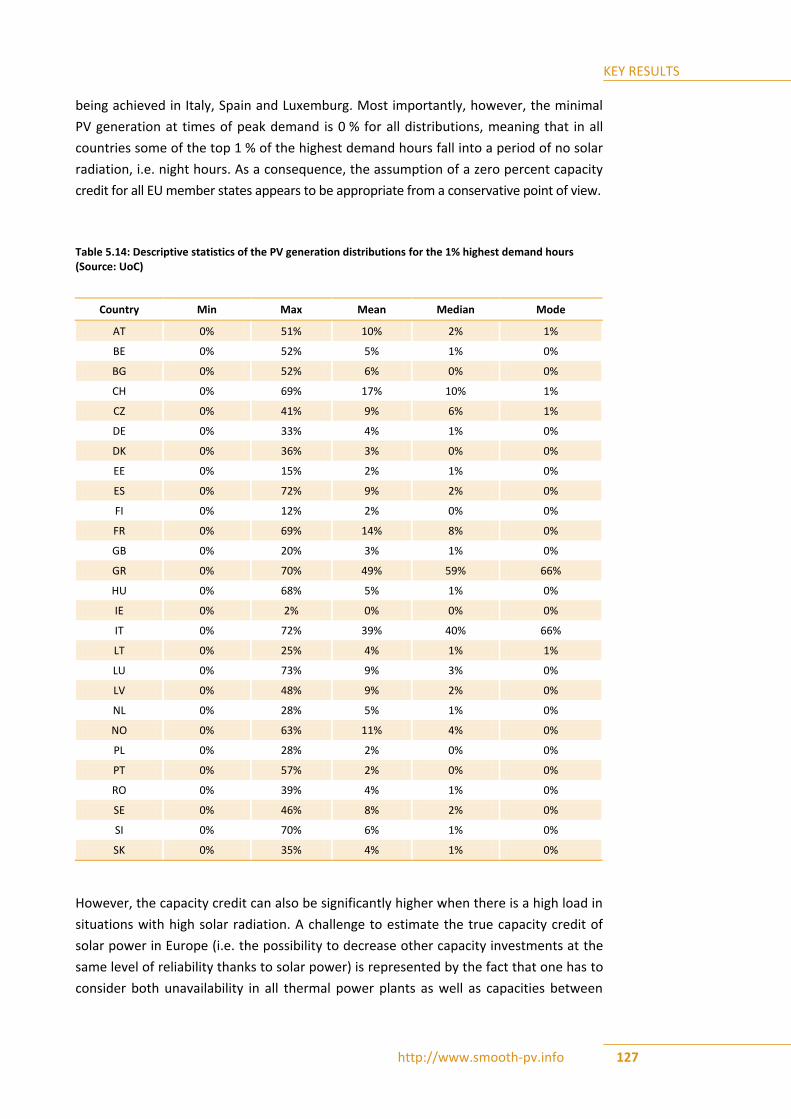
KEY RESULTS


being achieved in Italy, Spain and Luxemburg. Most importantly, however, the minimal

PV generation at times of peak demand is 0 % for all distributions, meaning that in all

countries some of the top 1 % of the highest demand hours fall into a period of no solar

radiation, i.e. night hours. As a consequence, the assumption of a zero percent capacity

credit for all EU member states appears to be appropriate from a conservative point of view.

Table 5.14: Descriptive statistics of the PV generation distributions for the 1% highest demand hours (Source: UoC)

Country Min Max Mean Median Mode

AT 0% 51% 10% 2% 1%

BE 0% 52% 5% 1% 0%

BG 0% 52% 6% 0% 0%

CH 0% 69% 17% 10% 1%

CZ 0% 41% 9% 6% 1%

DE 0% 33% 4% 1% 0%

DK 0% 36% 3% 0% 0%

EE 0% 15% 2% 1% 0%

ES 0% 72% 9% 2% 0%

FI 0% 12% 2% 0% 0%

FR 0% 69% 14% 8% 0%

GB 0% 20% 3% 1% 0%

GR 0% 70% 49% 59% 66%

HU 0% 68% 5% 1% 0%

IE 0% 2% 0% 0% 0%

IT 0% 72% 39% 40% 66%

LT 0% 25% 4% 1% 1%

LU 0% 73% 9% 3% 0%

LV 0% 48% 9% 2% 0%

NL 0% 28% 5% 1% 0%

NO 0% 63% 11% 4% 0%

PL 0% 28% 2% 0% 0%

PT 0% 57% 2% 0% 0%

RO 0% 39% 4% 1% 0%

SE 0% 46% 8% 2% 0%

SI 0% 70% 6% 1% 0%

SK 0% 35% 4% 1% 0%

However, the capacity credit can also be significantly higher when there is a high load in

situations with high solar radiation. A challenge to estimate the true capacity credit of

solar power in Europe (i.e. the possibility to decrease other capacity investments at the

same level of reliability thanks to solar power) is represented by the fact that one has to

consider both unavailability in all thermal power plants as well as capacities between


KEY RESULTS


the different areas, since power can be traded also during peak load situations. It is also

important to note that just because a power plant sometimes does not provide power

during peak load, this does not necessarily mean that its capacity credit is zero, as this

would imply that all power plants have capacity credit equal to zero since they

sometimes fail.

5.5.2 The Economic Inefficiency of Grid Parity: The Case of German Photovoltaics in

Scenarios until 2030

Due to massive reductions in the price for photovoltaic (PV) systems, PV grid parity has

recently been reached in Germany. PV grid parity on the household level is defined as the

point in time at which the levelized costs of PV reach parity with the residential electricity

tariff. As PV system prices continue to decrease (and the residential electricity tariff

continues to increase), the gap between the levelized costs of electricity (LCOE) of PV and

the retail electricity tariff will grow and trigger investments in residential PV systems -

even in the absence of any direct financial incentives such as solar power feed-in tariffs.

However, while the single household can lower its annual electricity costs through

investments in rooftop PV systems, the partial optimization of the single household is

inefficient from an economic perspective. Households optimize their PV investments by

comparing the LCOE of PV to the residential electricity tariff that includes network

tariffs, taxes, levies and other surcharges that can be avoided when consuming self-

produced PV electricity instead of purchasing electricity from the grid. Therefore, private

investments in rooftop PV systems receive an indirect financial incentive in the current

regulatory environment.

In this study, we have analyzed the consequences of PV grid parity in Germany until

2030 from both the single household and the wholesale market perspective. This was

done by iterating the dynamic linear electricity system optimization model (explained in

Section 4.3) with a household optimization model. The approach is described in detail in

the paper in [App03].

5.5.2.1 Methodology

The household optimization model minimizes the annual electricity costs of households,

given yearly solar irradiance and electricity consumption profiles, PV and storage system

investment costs, residential electricity tariffs and hourly market values of PV electricity

generation. The model in turn determines the optimal PV and storage system capacities

from the single household perspective – depending on the number of residents living in

the house (1-5 residents) and the location of the house (North-, Central- and South-

Germany) – as well as hourly system performance statistics, including hourly PV

electricity self-consumption and grid feed-in profiles.


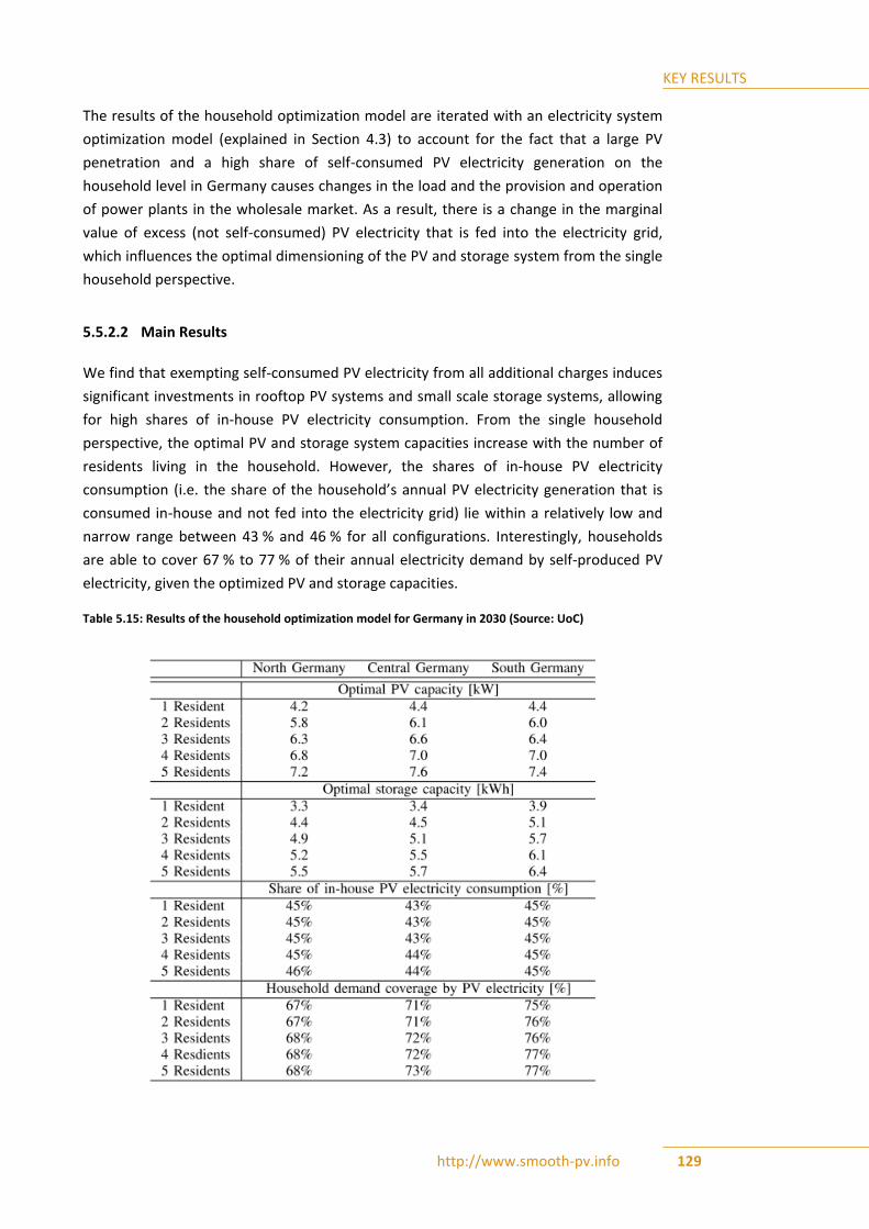
KEY RESULTS


The results of the household optimization model are iterated with an electricity system

optimization model (explained in Section 4.3) to account for the fact that a large PV

penetration and a high share of self-consumed PV electricity generation on the

household level in Germany causes changes in the load and the provision and operation

of power plants in the wholesale market. As a result, there is a change in the marginal

value of excess (not self-consumed) PV electricity that is fed into the electricity grid,

which influences the optimal dimensioning of the PV and storage system from the single

household perspective.

5.5.2.2 Main Results

We find that exempting self-consumed PV electricity from all additional charges induces

significant investments in rooftop PV systems and small scale storage systems, allowing

for high shares of in-house PV electricity consumption. From the single household

perspective, the optimal PV and storage system capacities increase with the number of

residents living in the household. However, the shares of in-house PV electricity

consumption (i.e. the share of the household’s annual PV electricity generation that is

consumed in-house and not fed into the electricity grid) lie within a relatively low and

narrow range between 43 % and 46 % for all configurations. Interestingly, households

are able to cover 67 % to 77 % of their annual electricity demand by self-produced PV

electricity, given the optimized PV and storage capacities.

Table 5.15: Results of the household optimization model for Germany in 2030 (Source: UoC)


KEY RESULTS


Figure 5.50 shows the average share of the (daily) household electricity demand that can

be covered by self-produced PV electricity during summer and winter in scenario A. On

average, households are able to cover up to 96 % of their daily electricity demand by

self-produced PV electricity in the summer, and up to 80 % in the winter.

Figure 5.50: Average daily residential electricity demand coverage by self-produced PV electricity in Germany in 2030 (Source: UoC)

The single household's optimization behavior entails direct consequences for the

wholesale market. As shown in Figure 5.51 and Figure 5.52, high shares of in-house PV

electricity consumption on the single household level cause significant changes in the

load supplied by the wholesale electricity market (residual load).13

Figure 5.51: Average (residual) load on weekdays in the summer and the winter in Germany in 2030 (Source: UoC)

..............................

13 In this analysis, the term ‘residual load’ corresponds to Germany’s total electricity demand (load) without

the accumulated in-house PV electricity consumption on the household level.


KEY RESULTS


On average, the load supplied by the wholesale electricity market on weekdays

decreases by up to 12 % in the summer, and by up to 8 % in the winter due to in-house

PV electricity consumption. Interestingly, the highest load reduction on weekdays occurs

in the evening hours, due to the in-house consumption of PV electricity that was stored

in battery systems during the day. 14

Figure 5.52: Average load reduction on weekdays through in-house PV electricity consumption in the summer and the winter in Germany in 2030 (Source: UoC)

From an economic perspective, the partial optimization of the single households

(induced by PV grid parity) leads to significant excess costs. In comparison to the cost-

optimal solution achieved under a total system optimization (which ensures the cost-

efficient development of Germany's electricity generation mix up to 2030), accumulated

and discounted total system costs increase by 7.1 bn €2011 up until 2030. This massive

increase in total system costs is caused by the fact that investments in rooftop PV

systems and small scale storage technologies (such as lithium-ion batteries) on the single

household level do not depict a cost-efficient investment option in Germany before

2030.

The paper is included in [App03].

..............................

14 However, since Figure 5.51 and Figure 5.52 show the average load reduction on weekdays during summer

and wintertime, it cannot be concluded that peak load is reduced. For such a conclusion, specific instances

in time would need to be analyzed in detail. This is subject to further research.


6 CONCLUSIONS &

FUTURE WORK

CONCLUSIONS


6. CONCLUSIONS AND FUTURE WORK

6.1 CONCLUSIONS

6.1.1 Issues in the Transmission Network

In the transmission system high penetration of PV raises concerns regarding the

adequacy of the available generation resources. PV output varies both in a deterministic

manner (day/night, summer/winter) and in a stochastic manner (due to clouds, for

example). While the former is completely predictable and can be accounted for in the

planning process of the generation and transmission infrastructures, which need to be

able to accommodate high amounts of PV and the associated ramp rates in the

mornings and evenings, the latter is influenced by the balancing area size. It has been

shown that the aggregation of several PV plants dispersed geographically leads to a

smoothing of the aggregated output, as cloud formations are typically non-homogenous

and have a limited velocity above ground. Hence the larger the balancing area

containing a number of plants, the less flexibility reserves in the form of flexible power

plants, grid, storage and flexible demand are required.

On the pan-European level a simulation study showed that about 30-40 % of yearly

consumption can be feasibly covered by PV while keeping the curtailed amount low and

the necessary storage amount feasible, without even making any major extensions to

the transmission system.

In a parallel study, detailed scenarios for the future development of both generation and

transmission system infrastructures in Europe were worked out using a long-term

investment and dispatch model for renewable, conventional, storage and transmission

technologies (the Electricity Market Model) and a Transmission System Model. The

models cover 29 countries and are capable of simulating how installed capacities and

their operation will develop in the future given a set of assumptions regarding techno-

economic conditions as well as the regulatory framework. They consider detailed load

flow simulations in those countries, including the operation of HVDC lines in meshed AC

networks and a HVDC SuperGrid across Europe. An algorithm was developed that allows

optimizing power generation and transmission infrastructures jointly through an

iterative approach based on power transfer distribution factors (PTDFs). It proved to be

applicable and convergent for both small scale and large scale models. In a large scale

application dealing with the European power system it was found that there is a

significant cost-difference of 591 bn. € (20.9 %) between a scenario with optimal

transmission grid extensions and a scenario strictly avoiding transmission grid

extensions. This result clearly demonstrates that significant grid extensions help to cost-

efficiently deploy renewable power sources across Europe.


CONCLUSIONS


The capacity credit of PV, measuring the contribution of PV to the system’s security of

supply, was found to be 0 % for all EU member states from a conservative point of view,

due to an electricity demand structure that is characterized by high levels during

evening hours when no PV generation is available.

PV grid parity on the household level has recently been reached in Germany, thus

triggering investments in residential PV systems. Whereas from a household point of

view, the optimal PV and storage system capacities increase with the number of

residents in the household - enabling them to cover on average 72 % of their annual

electricity demand by self-produced PV electricity in 2030 - the economic inefficiency

caused by the partial optimization of single households (induced by PV grid parity) leads

to significant excess costs of 7.1 bn. €2011 in 2030 compared to the cost-optimal solution

achieved under a total system optimization.

PV needs to provide ancillary services on all voltage levels. These capabilities are

typically regulated through Grid Codes, which apply throughout distribution and

transmission networks. One important requirement is related to the 50.2 Hz issue, the

frequency value that, if reached, would cause several gigawatts of PV to disconnect from

the grid and thus jeopardize the security of supply. The problem has been recognized

and there are currently retrofitting activities in place.

6.1.2 Issues in the Distribution Network

The principal issues encountered in the distribution systems are related to voltage

control, equipment loading and power quality. In the course of the Smooth PV project,

models of PV, electrical storage (for a Vanadium Redox Flow battery) and a small office

building with responsive demand were developed and validated and then used for

studies of the impact of PV in the distribution grid.

Using these models a number of voltage control strategies were implemented in

Matlab/Simulink and DIgSILENT PowerFactory. The strategies include methods based on

reactive power (voltage droop and active power droop) and on active power through

shifting load and utilizing battery storage.

The reactive power methods are droop based and use local measurements for the

reactive power set-point. The first method, active power-dependent, uses the local

active power production to issue the reactive power set-point. This method does not

address the voltage directly, but has the advantage of simplicity. The second method,

droop-based voltage control, gives the reactive power set-point based on the local

voltage measurement. For this method, care must be taken to coordinate the actions of

nearby systems, so that there are no negative interactions between them. Both

methods show better performance, such as lower reactive power consumption and a

better voltage profile, than the standard German Grid Code. It has also been established

that the R/X ratio has a large impact and a higher ratio reduces the impact of reactive

power control on the voltage.


CONCLUSIONS


With the help of active power control, load shifting is an effective measure to avoid

overvoltages, especially in LV networks with high R/X ratios. The same applies to

electrical storage that can be charged/discharged depending on the voltage or

scheduled to charge at specific times when PV is expected to produce electricity. The

method of load shifting is preferable in cases where manageable loads are available,

which can then be utilized to provide a cheap and effective solution to voltage control

problems. The second method of using storage to assist with voltage control is relevant

where the production of the PV plants exceeds the local consumption to such a degree

that an investment in a storage unit is necessary.

Power quality issues were studied using a developed model for harmonic analysis based

on laboratory measurements. The model includes both the emission of inverters and the

influence of their output impedance on the resonances in the system. A case study of a

LV network with a large number of inverters was analyzed for this purpose. The

aggregation of harmonic currents of multiple inverters was analyzed based on a field

measurement, and a modification of the existing summation coefficients was proposed

for the case of PV inverters.

Fault-Ride-Through capability and voltage support provided by inverters during short-

circuits in the distribution network was analyzed based on dynamic computer

simulations. It was found that inverters offer very limited voltage support if their current

is limited to a value close to the nominal.


FUTURE WORK


6.2 FUTURE WORK

6.2.1 Coupling of the Transmission Grid Model and the Economic Market Model for

System Planning Studies

The coupling of the physical model of the transmission grid with the economic market

model could be further developed in various directions. With respect to the

optimization, several interesting possibilities are outlined below:

The optimization could be reformulated as a mixed integer problem, so that only

multiples of available line configurations and power station capacities can be

added, rather than using continuous variables for all quantities.

Modeling also non-linear quantities would allow the optimization to also take

account of thermal losses and to avoid the iteration by recalculating the PTDFs

directly from the line impedances.

Higher time resolution would enable the optimization to consider longer extreme

weather events that really stress the power system.

Further spatial disaggregation towards a nodal-pricing regime would overcome the

difficulty of having an unequal number of nodes in the power flow and market

model.

On the modeling side, to avoid voltage angle instability problems, the voltage angle

could be tracked even in a linear optimization problem so that differences between

busses could be limited to, for example, 30-40°.

Including a certain amount of demand-side management would help avoid some of the

high costs incurred by storage.

It would also be interesting to consider a scenario intermediate between the optimal

and minimal grid extension scenarios considered above. For example, a more expensive

transmission line price could be justified by including the costs of a lack of social

acceptance for pylons. In a similar vein, another scenario could allow only HVDC line

extensions, which can also be built as underground cables.

Furthermore, it could be analyzed numerically how gains in social welfare can be created

when switching the congestion management from NTC to flow-based market coupling.

Whereas the principal effects have been analyzed theoretically in a number of studies,

the issue has never been analyzed for the Pan-European context based on a model with

high spatial, temporal and technological resolution.

In the same vein, the methodology could be applied to smaller subsystems, which would

allow for a higher regional and temporal resolution while still being able to handle the

complexity of the calculation.


FUTURE WORK


With regard to the capacity credit of PV, the calculation could alternatively be built on

reliability-based methods, such as the Effective Load-Carrying Capability (ELCC) or the

Equivalent Firm Power (EFP) method.]

6.2.2 Voltage Control in the Distribution Grids

Control algorithms could be further tested and validated using SYSLAB facilities. Also,

new voltage and power control strategies and controllers for distribution networks with

high shares of PV systems could be developed and validated.

6.2.3 Power Quality in Distribution Networks

As discussed in section 5.3.2, the trend of new models of PV inverters is towards very

low emission of harmonic currents (5 % current THD). This limits their impact on the

harmonic voltages in terms of generated current. However, the equivalent impedance of

inverters needs to be taken into account because it has an influence on the network

resonances. Most inverters show capacitive behavior, which leads to a decrease of the

frequency of the first parallel resonance. Filter topologies of inverters should be

considered in the future as a solution of this problem in a scenario with very high PV

penetration levels.

Regarding voltage support during voltage dips (network faults), it was shown that PV

inverters offer very little voltage support if their current is limited to close to a nominal

value. The fault ride through capability of inverters should be explored more in the

future, considering possible implications on the connection requirements, which would

provide more voltage support to networks with a high PV generation share.

This question should be investigated further in terms of fault ride through requirements

for inverters, which would prevent a significant increase in the number and depth of

voltage dips in a scenario where a large number of synchronous generators are

substituted by inverter-interfaced generators.

6.2.4 Inertia Issues Related to High Share of PV

An important consideration that needs careful study is related to power systems which

have very high instantaneous PV (or any other non-synchronous generation) penetration

levels. Limits are imposed by the necessary amount of spinning reserves, the minimum

allowed operating limits of the thermal plants and their ramping capabilities. Non-

synchronous generation may need to provide synthetic inertia and short-circuit

currents, and thereby contribute to frequency and voltage stability and help operate

protection devices.


FUTURE WORK


Going even further, systems with 100 % penetration, i.e. 100 % non-synchronous

generation, and especially their control, are likely to come under consideration in

coming years.

6.2.5 Grid Code Issues / 50.2 Hz Issue

As discussed in section 3.4.5 a large number of inverters connected at low voltage are

currently configured to disconnect from the grid if the mains frequency exceeds 50.2 Hz.

This particularly applies to countries with high instantaneous penetration levels, such as

Germany. In Germany, the system stability act introduced in 2012 dictates that PV

systems bigger than 10 kW must be reconfigured to withstand frequency rise events

above 50.2 Hz by the end of 2014. Systems above 100 kW must be retrofitted by

31.08.2013. Until then system stability could be jeopardized, especially on sunny

weekends in the upcoming summer when the system load is low and simultaneously PV

production in the system is high.

6.2.6 Operational Issues

There are concerns that PV systems could sustain an undesired island network in a

distribution grid if their production is closely matched to the load in the subsystem. This

is so-called ‘unintentional islanding’. Due to this issue, a limit exists, for example in the

USA, which stipulates a certain (low) percentage of maximum allowed installed PV

capacity on a feeder in relation to the load on this feeder. The unintentional islanding

problem may need further careful consideration.

Operation of protection equipment and its settings might need to be readjusted as the

system structure undergoes changes related to large amounts of PV and other inverter-

coupled generation.


7 BIBLIOGRAPHY

BIBLIOGRAPHY


7. BIBLIOGRAPHY

[1] EuroWind, 2011. Database for hourly wind speeds and solar radiation from 2006-

2010 (not public). EuroWind GmbH.

[2] Richter, J., 2011. Electricity market model description (Working Paper) University of

Cologne.

[3] Golling, C., 2011: A Cost-Efficient Expansion of Renewable Energy Sources in the

European Electricity System – An Integrated Modelling Approach with a Particular

Emphasis on Diurnal and Seasonal Patterns. Dissertations

[4] German Energy Agency, 2005: Planning of the Grid Integration of Wind Energy in

Germany Onshore and Offshore up to the Year 2020 (dena Grid study)

[5] TradeWind, 2008: Integrating Wind Developing Europe’s power market for the large-

scale integration of wind power, WP2.6 – Equivalent Wind Power Curves

[6] Eicker, U., 2001: Solare Technologien für Gebäude, B.G. Teubner Verlag

[7] Quaschning, V., 2000: Systemtechnik einer klimaverträglichen Elektrizitätsversorgung

in Deutschland für das 21. Jahrhundert, Forschritt-Berichte VDI, Reihe 6, Nr. 437, VDI-

Verlag Düsseldorf 2000

[8] British Geological Survey, 2008: Mineral Planning Factsheet – Underground Storage

[9] Oertel, D., 2008: Energiespeicher – Stand und Perspektiven. Büro für Technikfolgen-

Abschätzung beim Deutschen Bundestag

[10] Gillhaus, A., 2008: Natural gas storage in salt caverns – present status, develop-

ments and future trends in Europe

[11] IFEU Heidelberg, 2009: Wasserstoff- und Stromspeicher in einem Energiesystem mit

hohen Anteilen erneuerbarer Energien: Analyse der kurz- und mittelfristigen Perspektive

[12] Ehlers, U., 2005: Windenergie und Druckluftspeicher. Netzentlastung und Reserve-

stellung mit Druckluftspeicher im Rahmen einer deutschen Elektrizitätsversorgung mit

hohem Windenergieanteil.

[13] European Commission - Joint Research Centre- Institute for Energy and Transport

(2011): Technology Map of the European Strategic Energy Technology Plan

[14] Amelin, M., 2009: Comparison of Capacity Credit Calculation Methods for Conven-

tional Power Plants and Wind Power, IEEE Transactions on Power Systems, Vol. 24, No. 2

[15] Hansen, T.,2007: Utility Solar Generation Valuation Methods, USDOE Solar America

Initiative

[16] Progress Report, Tucson Electric Power, Tucson, AZ.


BIBLIOGRAPHY


[17] Hoff, T., R. Perez, J.P. Ross and M. Taylor, 2008: Photovoltaic Capacity Valuation

Methods, SEPA REPORT # 02-08, Washington, DC, Solar Electric Power Association.

[18] International Energy Agency, 2011: World Energy Outlook 2011, OECD Publishing.

[19] Bartels, M., 2009. Cost Efficient Expansion of District Heat Networks in Germany.

Oldenbourg Industrieverlag.

[20] Nagl, S., Fürsch, M., Paulus, M., Richter, J., Trüby, J., Lindenberger, D., 2011. Energy

Policy Scenarios to Reach Challenging Climate Protection Targets in the German

Electricity Sector until 2050. Utilities Policy, 19(3), pp. 185-192.Richter, J., 2011.

Electricity market model description (Working Paper) University of Cologne.

[21] Schlesinger, M., Hofer, P., Kemmler, A., Kirchner, A., Strassburg, S., Lindenberger,

D., Fürsch, M., Nagl, S., Paulus, M., Richter, J., Trüby, J., 2010. Energieszenarien f¨ur ein

Energiekonzept der Bundesregierung (in German).Tech. rep., Prognos AG,

Energiewirtschaftliches Institut an der Universität zu Köln and GWS mBh.

[22] ENTSO-E, 2012: Hourly load values of a specific country for a specific month.

European Network of Transmission System Operators for Electricity.

[23] A. Medina, “Harmonic simulation techniques (methods & algorithms),” in IEEE

Power Engineering Society General Meeting, 2004., vol. 2, pp. 762–765.

[24] A. Medina, N. R. Watson, P. F. Ribeiro, and C. J. Hatziadoniu, “Harmonic analysis in

frequency and time domains, Harmonic Modeling Tutorial, Chapter 5.”

[25] I. T. Papaioannou, M. C. Alexiadis, C. S. Demoulias, D. P. Labridis, and P. S.

Dokopoulos, “Modeling and Field Measurements of Photovoltaic Units Connected to LV

Grid. Study of Penetration Scenarios,” IEEE Transactions on Power Delivery, vol. 26, no.

2, pp. 979–987, Apr. 2011.

[26] J. L. Agorreta, M. Borrega, J. López, and L. Marroyo, “Modeling and Control of N-

Paralleled Grid-Connected Inverters With LCL Filter Coupled due to Grid Impedance in

PV Plants,” IEEE Transactions on Power Electronics, vol. 26, no. 3, pp. 770–785, Mar.

2011.

[27] C. Ong, “Operational Behavior of Line-Commutated Photovoltaic Systems on a

Distribution Feeder,” IEEE Transactions on Power Apparatus and Systems, vol. PAS-103,

no. 8, pp. 2262–2268, Aug. 1984.

[28] M. C. Benhabib, J. M. A. Myrzik, and J. L. Duarte, “Harmonic effects caused by large

scale PV installations in LV network,” in 2007 9th International Conference on Electrical

Power Quality and Utilisation, 2007, pp. 1–6.

[29] G. Campen, “An Analysis of the Harmonics and Power Factor Effects at a Utility

Intertied Photovoltaic System,” IEEE Transactions on Power Apparatus and Systems, vol.

PAS-101, no. 12, pp. 4632–4639, Dec. 1982.


BIBLIOGRAPHY


[30] J. H. R. Enslin and P. J. M. Heskes, “Harmonic Interaction Between a Large Number

of Distributed Power Inverters and the Distribution Network,” IEEE Transactions on

Power Electronics, vol. 19, no. 6, pp. 1586–1593, Nov. 2004.

[31] N. Jayasekara and P. Wolfs, “Analysis of power quality impact of high penetration

PV in residential feeders.”

[32] H. Oldenkamp, I. de Jon, P. J. M. Heskes, P. M. Rooij, and H. H. C. de Moor,

“Additional requirements for PV inverters necessary to mantain utility grid quality in

case of high penetration of PV generators,” in 19th European PV Solar Energy Confe-

rence and Exibition, 2004.

[33] A. J. A. Bosman, J. F. G. Cobben, J. M. A. Myrzik, and W. L. Kling, “Harmonic

Modelling of Solar Inverters and Their Interaction with the Distribution Grid,” in

Proceedings of the 41st International Universities Power Engineering Conference, 2006,

vol. 3, pp. 991–995.

[34] V. Ćuk, P. F. Ribeiro, J. F. G. Cobben, W. L. Kling, F. R. Isleifsson, H. W. Bindner, N.

Martensen, A. Samadi, and L. Söder, “Considerations on the modeling of photovoltaic

systems for grid impact studies,” in 1st International Workshop on the Integration of

Solar Power into Power Systems, 2011.

[35] IEC/TR61000-3-14, “Electromagnetic compatibility (EMC) - Part 3-14: Assessment of

emission limits for the connection of disturbing installations to LV power systems,”

2011.

[36] W. G. Sherman, “Summation of harmonics with random phase angles,” Proceedings

of the Institution of Electrical Engineers, vol. 119, no. 11, p. 1643, 1972.

[37] S. R. Kaprielian, A. E. Emanuel, R. V. Dwyer, and H. Mehta, “Predicting voltage

distortion in a system with multiple random harmonic sources,” IEEE Transactions on

Power Delivery, vol. 9, no. 3, pp. 1632–1638, Jul. 1994.

[38] Y. Baghzouz, R. F. Burch, A. Capasso, A. Cavallini, A. E. Emanuel, M. Halpin, R.

Langella, G. Montanari, K. J. Olejniczak, P. Ribeiro, S. Rios-Marcuello, F. Ruggiero, R.

Thallam, A. Testa, and P. Verde, “Time-varying harmonics. II. Harmonic summation and

propagation,” IEEE Transactions on Power Delivery, vol. 17, no. 1, pp. 279–285, 2002.

[39] J. Schlabbach, G. Chicco, and F. Spertino, “Operation of multiple inverters in grid-

connected large-size photovoltaic installations.”

[40] E. Vasanasong and E. D. Spooner, “The effect of net harmonic currents produced by

numbers of the Sydney Olympic Village’s PV systems on the power quality of local

electrical network,” in PowerCon 2000. 2000 International Conference on Power System

Technology. Proceedings (Cat. No.00EX409), 2000, vol. 2, pp. 1001–1006.

[41] A. C. Ernauli, “Modeling of photovoltaic inverters for power quality studies,”

Eindhoven University of Technology, 2012.

[42] J. Feng, “Dynamic behavior of grid-connected inverters during voltage dips,” 2011.


BIBLIOGRAPHY


[43] B. Renders, K. De Gusseme, W. R. Ryckaert, K. Stockman, L. Vandevelde, and M. H. J.

Bollen, “Distributed Generation for Mitigating Voltage Dips in Low-Voltage Distribution

Grids,” IEEE Transactions on Power Delivery, vol. 23, no. 3, pp. 1581–1588, Jul. 2008.

[44] IEC61000-3-6, “Electromagnetic compatibility (EMC) - Part 3-6: Limits - Assesment

of emission limits for the connection of distorting installations to MV, HV, and EHV

power systems,” 2008.

[45] A. Constantin, R. D. Lazar, J. Dannehl, S. . Kjaer, and M. Ibsch, “Calculation of

harmonic current content in PV power plants based on single inverter data,” in 1st

International Workshop on the Integration of Solar Power into Power Systems, 2011.

[46] J. Lava, J. F. G. Cobben, W. L. Kling, and F. Overbeeke, “Addressing LV network

power quality issues through the implementation of a microgrid,” in International

Conference on Renewables and Power Quality 2010, 2010.

[47] V. Cuk, J. F. G. Cobben, W. L. Kling, and P. F. Ribeiro, “Considerations on harmonic

impedance estimation in low voltage networks,” in 2012 IEEE 15th International

Conference on Harmonics and Quality of Power, 2012, pp. 358–363.

[48] Mills, A. et al “Understanding Variability and Uncertainty of Photovoltaics for

Integration with the Electric Power System”, Ernest Orlando Lawrence Berkeley National

Laboratory, December 2009

[49] An online press release:

http://www.younicos.com/en/media_library/press_releases/011_1MWPCM-Vattenfall.html

[50] Wirth, H. “Aktuelle Fakten zur Photovoltaik in Deutschland”, Fraunhofer ISE,

Version of January 8, 2013

[51] VDE ETG-Task Force Demand Side Management “Demand Side Integration.

Lastverschiebungspotenziale in Deutschland”, June 2012

[52] ENTSOE-E, Network Code on Requirements for Grid Connection applicable to all

Generators, available online at: https://www.entsoe.eu/major-projects/network-code-

development/requirements-for-generators/

[53] M. Fürst, „Das 50,2 Hz-Problem“, EnBW Transportnetze AG, 2011

http://www.vde.com/de/fnn/arbeitsgebiete/tab/documents/fuerst_50-2-hz-problem.pdf

[54] Weißbach, T.; Welfonder, E. (2011): Große Frequenzabweichungen im europäischen

Verbundnetz. Teil 1: Leistungsungleichgewicht im Strommarkt. In: Ew 110 (5), S. 36–40.

[55] Weißbach, T. „Verbesserung des Kraftwerks- und Netzregelverhaltens bezüglich

handelsseitiger Fahrplanänderungen“, Dissertation, Stuttgart 2009

[56] Bundesrat „Verordnung zur Gewährleistung der technischen Sicherheit und

Systemstabilität des Elektrizitätsversorgungsnetzes (Systemstabilitätsverordnung –

SysStabV), May 2012


http://www.younicos.com/en/media_library/press_releases/011_1MWPCM-Vattenfall.html

https://www.entsoe.eu/major-projects/network-code-development/requirements-for-generators/

https://www.entsoe.eu/major-projects/network-code-development/requirements-for-generators/

http://www.vde.com/de/fnn/arbeitsgebiete/tab/documents/fuerst_50-2-hz-problem.pdf

BIBLIOGRAPHY


[57] ENTSO-E “Ten-Year Network Development Plan 2012”, available online at:

https://www.entsoe.eu/major-projects/ten-year-network-development-plan/tyndp-2012/

[58] Zickfeld, F. et al. “2050 Desert Power”, Dii GmbH, First Edition, June 2012

[59] Ackermann, T., Kuwahata, R. “Lessons Learned from International Wind Integration

Studies”, Energynautics GmbH, Germany, November 2011

[60] Ellis, A. et al. „Model Makers“, IEEE power & energy magazine, May/June 2011

[61] S@tel-Light, an online database, available at: http://www.satel-light.com/

[62] Renewable Resource Data Center, an online database, available at:

http://www.nrel.gov/rredc/

[63] Jewell, W., Ramakumar, R. “The Effects of Moving Clouds in Electric Utilities with

Dispersed Photovoltaic Generation”, IEEE Transactions on Energy Conversion, Vol. EC-2,

No. 4, December 1987

[64] ENTSO-E, an online data portal, available at https://www.entsoe.eu/data/data-

portal/

[65] Grid study „Roadmap 2050 – a closer look“, available online at:

http://www.energynautics.com/aktuelles/Roadmap_2050_komplett_Endbericht_Web.pdf

[66] European grid study 2030/2050 for Greenpeace International, available online at:

http://www.energynautics.com/downloads/europeangridstudy2030-

2050/energynautics_EUROPEAN-GRID-STUDY-2030-2050.pdf

[67] L. Mihet-Popa, C. Koch-Ciobotaru, F. Isleifsson and H. Bindner, “Simulation models

developed for storage systems with over voltage control for PV penetration in a

distribution network”, IEEE Transactions on Smart Grid-Special Issue: Energy storage

applications for smart grid, under review


https://www.entsoe.eu/major-projects/ten-year-network-development-plan/tyndp-2012/

http://www.satel-light.com/

http://www.nrel.gov/rredc/

https://www.entsoe.eu/data/data-portal/

https://www.entsoe.eu/data/data-portal/

http://www.energynautics.com/aktuelles/Roadmap_2050_komplett_Endbericht_Web.pdf

http://www.energynautics.com/downloads/europeangridstudy2030-2050/energynautics_EUROPEAN-GRID-STUDY-2030-2050.pdf

http://www.energynautics.com/downloads/europeangridstudy2030-2050/energynautics_EUROPEAN-GRID-STUDY-2030-2050.pdf

8 APPENDIX

APPENDIX


8. APPENDIX

The appendix at hand contains the scientific papers and reports that include detailed

description of the methodologies applied and results achieved by the participating parties

within the Smooth PV project. Click here for the papers/reports published on our website.

Paper / Report Participant Milestone Reference in the report

Transporting Renewables: Systematic Planning for Long-Distance HVDC Lines

Energynautics 2 App01

Determining the Maximum Feasible Amount of Photovoltaics in the European Transmission Grid Under Optimal PV Utilization

Energynautics 4 App02

The economic inefficiency of grid parity: The case of German photovoltaics in scenarios until 2030

UoC 6 App03

Cost-optimal Power System Extension Under Flow-based Market Coupling and High Shares of Photovoltaics

UoC, Energynautics

4, 8 App04

Development of Tools for DER Components in a Distribution Network

DTU 10 App05

Simulation Model developed for a Small-Scale PV System in Distribution Networks

DTU 10 App06

Development of Tools for Simulation Systems in a Distribution Network and Validated by Measurements

DTU 11 App07

Development, Improvements and Validation of a PV System Simulation Model in a Micro-Grid

DTU 11 App08

Model Predictive Controller for Active Demand Side Management with PV Self-consumption in an Intelligent Building

DTU 12 App09

Characterisation of the rapid fluctuation of the aggregated power output from distributed PV panels

DTU 12 App10

Comparison of a Three-Phase Single-Stage PV System in PSCAD and PowerFactory

KTH 14, 15 App11

Comparison of a Three-Phase Single-Stage PV System in PSCAD and PowerFactory (Master Thesis, provided as a separate file on the website)

KTH 14, 15 App12

Improving the Photovoltaic Model in PowerFactory (Master Thesis, provided as a separate file on the website)

KTH 14, 15 App13

Coordinated Droop Based Voltage Control among PV Systems in Distribution Grids

KTH 16 App14

Equivalent modelling of several PV power plants

KTH 16 App15


http://www.smooth-pv.info/publications.html

APPENDIX


Paper / Report Participant Milestone Reference in the report

Evaluation of Reactive Power Support Interactions Among PV Systems Using Sensitivity Analysis

KTH 16 App16

Modeling the Frequency Response of Photovoltaic Inverters

TUE 18 App17

Dynamic behavior of grid-connected inverters during voltage dips (Traineeship report, provided as a separate file on the website)

TUE 18 App18

Modeling of photovoltaic inverters for power quality studies (Master Thesis, provided as a separate file on the website)

TUE 19 App19

Considerations on Harmonic Impedance Estimation in Low Voltage Networks

TUE 20 App20

Aspects of a generic photovoltaic model examined under the German Grid Code for Medium Voltage

Energynautics Additional App21

Evaluating the Impact of PV Module Orientation on Grid Operation

Energynautics Additional App22

Considerations on the Modeling of Photovoltaic Systems for Grid Impact Studies

TUE, DTU, KTH, Energynautics

Additional App23

Variability and smoothing effects of PV power production

KTH Additional App24


SMART MODELING OF OPTIMAL INTEGRATION OF HIGH ......CCGT Combined Cycle Gas Turbine CCS Carbon...

Documents

Transcript of SMART MODELING OF OPTIMAL INTEGRATION OF HIGH ......CCGT Combined Cycle Gas Turbine CCS Carbon...