Smart Control Strategies for Heat Pump Systems
89
Smart Control Strategies for Heat Pump Systems Davide Rolando Hatef Madani June 2018
Transcript of Smart Control Strategies for Heat Pump Systems

Smart Control Strategies for Heat
Pump Systems
Davide Rolando
Hatef Madani June 2018

1
Summary
Heat pump industry development has reached a mature state over the last 20 years and
improvement of units’ component such as compressors or heat exchangers is more and
more demanding. On the other hand, the computational power of electronic device has
been increasing together with storage capability. For these reasons, a growing interest
has been dedicated to the introduction of advanced features in the heat pump system
controllers in order to improve the overall system performance by enhancing the control
logic algorithms.
The EffSys Expand Project P18 “Smart Control Strategies for Heat Pump systems”
(hereafter P18) is a research project proposed to evaluate new control strategies that can
be potentially implemented in the controller of heat pump systems for single-family house
applications. The control strategies investigated aim at adapting the control parameters
to dynamic parameters such as people’s behavior and weather forecast data.
The final goal of the Project was the improvement of the annual system efficiency and the
minimization of the annual operating cost of the system exploiting predictive control
strategies.
Improved control solutions have been designed and developed for both new installations
and currently operating heat pump systems.
The obtained results show that significant improvements can be achieved while
maintaining the simplicity of the traditional control approach and avoiding the complexity
involved in the implementation of sophisticated control algorithms. The annual energy
saving that can be achieved with the proposed control methods is up to 9%.
The control approach proposed in the Project represents a pragmatic and innovative
solution that can be implemented in any heat pump installation and allows a considerable
annual reduction of energy consumption and CO2 emissions.

2
Sammanfattning
Värmepumparnas utveckling de senaste 20 åren har lett till att dessa nu nått en mogen
status och ytterligare förbättring av enheternas komponenter som kompressorer eller
värmeväxlare blir alltmer krävande.
Samtidigt har beräkningskraften och lagringskapaciteten för styr-och reglerenheter ökat.
Detta har lett till ett växande intresse för införandet av avancerade funktioner i
värmepumpens styrsystem för att förbättra systemets totala prestanda genom att
förbättra kontrollsystemet.
EffSys Expand Projekt P18 "Smarta kontrollstrategier för värmepumpsystem" är ett
forskningsprojekt som föreslogs för att utvärdera nya kontrollstrategier som potentiellt kan
implementeras i kontrollsystemet för värmepumpsystem för enfamiljshus. De undersökta
kontrollstrategierna syftar till att anpassa kontrollparametrarna till dynamiska parametrar
som människors beteende och väderprognosdata.
Projektets slutmål var att förbättra den årliga systemeffektiviteten och minimera de årliga
driftskostnaderna för systemet genom att utnyttja prediktiva kontrollstrategier.
Förbättrade kontroll lösningar har utformats och utvecklats för både nya installationer och
befintliga värmepumpsystem. De erhållna resultaten visar att betydande förbättringar kan
uppnås samtidigt som enkelheten hos den traditionella kontrollmetoden bibehålls och
man undviker komplexiteten som krävs i genomförandet av mer sofistikerade
kontrollalgoritmer.
Den årliga energibesparingen som kan uppnås med de föreslagna kontrollmetoderna är
upp till 9%. Kontrollmetoden som föreslås i projektet utgör en pragmatisk och innovativ
lösning som kan genomföras i vilken värmepumpinstallation som helst och medger en
betydande årlig minskning av energiförbrukningen och koldioxidutsläppen.

3
Acknowledgements
This Research Project has been carried out thank to the fundamental contributions of several Project Partners that are here acknowledged. Each contribution, in terms of interest, ideas, suggestions, devices, material and time, made the development of the Project possible.
In the following, each Project Partner is listed together with a brief description of the respective contribution.
Thermia Värmepumpar contributed to the Project providing measurement data from
heat pump installations, in addition to valuable suggestions, insights and feedbacks on
the development of heat pump control algorithms and strategies.
NIBE contributed providing measurement data from heat pump installations, valuable
suggestions and feedbacks.
IVT-Bosch contributed to the project with man-hours in terms of feedbacks and
suggestions.
ETM Kylteknik AB provided measurement devices, suggestions and valuable insights.
It also provided the access to a heat pump installation for direct field measurements.
Hesch GmbH provided control devices to be employed for testing purposes at KTH
Energy Technology Lab.
Electrotest AB provided valuable feedbacks, suggestions and ideas to contribute to the
development of innovative control strategies.
Nowab AB and Bengt Dahlgren contributed as consultants with valuable knowledge and
feedbacks on heat pump systems and heat pump control.
UPV Universitat Politècnica de València has been the academic partner of the Project
and supported the research activity with valuable discussions and ideas, in the frame of
a fruitful collaboration between KTH and UPV.

4
Contents Summary ......................................................................................................................... 1
Sammanfattning .............................................................................................................. 2
Acknowledgements ......................................................................................................... 3
1 Project background and motivation .......................................................................... 7
1.1 Overall objectives ............................................................................................... 8
2 Report structure ....................................................................................................... 9
2.1 Note on the report structure ............................................................................... 9
3 Heat pump system control: literature review (WP2) ............................................... 10
3.1 Traditional control ............................................................................................. 10
3.2 Advanced control ............................................................................................. 11
3.3 Downside of advanced predictive methods ...................................................... 12
3.4 The heat pump control vision in this Project ..................................................... 13
3.5 Publications (WP5) ........................................................................................... 14
4 Heating system modelling (WP3) ........................................................................... 15
4.1 Heat pump unit modelling ................................................................................ 16
4.2 Building modelling ............................................................................................ 16
4.2.1 Internal gains ............................................................................................. 17
4.2.2 Infiltration ................................................................................................... 17
4.2.3 External convective coefficient .................................................................. 19
4.3 Other sub-models ............................................................................................. 20
4.4 Heat Pump system layouts ............................................................................... 20
4.5 Model validation ............................................................................................... 22
5 The shortcomings of the conventional control methods (WP2, WP3) .................... 24
5.1 Heating curve: influence of daily solar radiation ............................................... 28
5.2 Heating curve: influence of ambient temperature evolution ............................. 29
5.3 Heating curve: influence of solar radiation, wind and internal gains ................. 31
5.4 Modelling of building packages ........................................................................ 36
5.5 Final remarks ................................................................................................... 37
5.6 Publication (WP5) ............................................................................................ 38
6 Improvement potential study (WP3) ....................................................................... 39

5
6.1 Research questions ......................................................................................... 39
6.2 Improvement potential: implementation ........................................................... 39
6.3 Results ............................................................................................................. 41
6.3.1 Domestic hot water consumption perfect prediction .................................. 42
6.3.2 Internal gain perfect prediction .................................................................. 43
6.3.3 Solar radiation perfect prediction ............................................................... 44
6.4 Final remarks ................................................................................................... 45
6.5 Publications (WP5) ........................................................................................... 46
7 Weather data for system control (WP3) ................................................................. 47
7.1 Research questions ......................................................................................... 47
7.2 City selection .................................................................................................... 47
7.3 Weather data sources ...................................................................................... 47
7.4 Application Program Interface (API) development ........................................... 50
7.5 Results and remarks ........................................................................................ 51
7.6 Publication (WP5) ............................................................................................ 52
8 Heating curve adjustment with daily solar radiation prediction model (WP3) ......... 53
8.1 Introduction ...................................................................................................... 53
8.2 Weather data overview: Stockholm annual profiles .......................................... 53
8.2.1 Overview of weather variables over one-month ......................................... 55
8.3 Daily solar radiation prediction: model development ........................................ 56
8.3.1 Estimation of the daily solar radiation ........................................................ 58
8.3.2 Heating curve adjustment with daily solar radiation prediction .................. 58
8.4 Results ............................................................................................................. 59
8.5 Publication (WP5) ............................................................................................ 63
9 Numerical method for heating curve automatic adjustment (WP3, WP4) ............... 64
9.1 Introduction ...................................................................................................... 64
9.2 Implementation ................................................................................................. 65
9.3 Remarks ........................................................................................................... 68
9.4 Publication ........................................................................................................ 68
10 Heat Pump heating systems: field monitoring and measurements (WP4) ........... 69
10.1 Field measurements: overview ..................................................................... 69

6
10.2 Additional field measurements ...................................................................... 70
10.3 Publications .................................................................................................. 71
11 Hardware-in-the-loop control: basic implementation (WP4) ................................ 72
12 Conclusions ......................................................................................................... 76
13 Future work ......................................................................................................... 78
References .................................................................................................................... 79
Scientific publications (WP5) ......................................................................................... 85
Msc Theses and other publications (WP5) .................................................................... 85
Public workshop (WP5) ................................................................................................. 87

7
1 Project background and motivation
In Europe, an average of 800k heat pump units per year have been installed in the last
10 years adding up to about 10 million units operating in 2017 [1]. Only in Sweden, the
heat pump represents the most popular heating system solution for residential buildings
and in 2017 over 1.7 million heat pump units have been estimated to be in operation [1],
[2]. Building heating systems are now accounting for about 40% of the total energy
consumption and according to recent European Directives, all new buildings constructed
after 2020 should be “near zero energy” [3]. The heating sector can contribute to the
largest portion of carbon savings by 2030 by retrofitting existing buildings with more
efficient heating systems [1]. At the current estimated refurbishment rate, the replacement
of oil and gas burners with heat pumps could potentially allow to save 15 to 90 million
tons of CO2 per year in Europe [1]. The highest potential for energy saving and reduction
of greenhouse emissions goals can be achieved by means of a concurrent improvement
of the heat pump system performance.
Heat pump industry reached a mature stage with progressive improvements in unit
manufacturing over the last decades. Further performance improvement of units’
component such as compressors or heat exchangers is becoming economically less and
less sustainable for manufacturers. On the other hand, the computational power of
electronic device has been increasing together with storage and connection capability.
For these reasons there has been a growing interest in the possibility to introduce
advanced features in the heat pump system controllers in order to improve the overall
system performance by enhancing the control logic algorithm.
For improving the annual efficiency of heat pump systems and reaching the full
thermodynamic potential of the systems, an appropriate capacity control technique must
be developed and adjusted for each unique installation [4]. Furthermore, it has been
proved that the development and the implementation of improved control techniques is
much more cost effective than developing the heating system equipment. In particular,
with the decreased costs of data processing, storage and communication over recent
years, the design and implementation of improved control techniques have become
feasible and accessible [5].

8
1.1 Overall objectives This project aims at investigating the potential for improvement of the annual efficiency of
heat pump system and reduction of the annual operating cost of the system by enhancing
the control approach commonly adopted in residential applications. Traditional control
insights and new control algorithms are discussed considering the information from
people behavior, weather measurements and forecast in order to reduce the annual
electricity consumption and maximize thermal comfort in single family house installations.

9
2 Report structure
Chapter 1 presents a short literature review on the heat pump control approaches
adopted in common practice and the control solutions available in literature. The content
of this Chapter is related to the Work Package 2 of Project application.
The approach adopted in the Project to study system control solution is based on the
system modelling. In Chapter 2 the details of the developed simulation models are
provided. The content of this Chapter is related to Work Package 2.
In Chapter 3 the insights of the conventional control approach adopted in heat pump
systems are discussed. This Chapter is related to the Work Packages 2 and 3 of the
Project application.
In Chapter 4 the implementation and results of the improvement potential study carried
on to investigate the possible implementation of new control strategies are presented.
This Chapter is related to Work Package 3.
Chapter 5 present the analysis carried out on the weather data sources that have been
considered for possible improvement of the system control. This Chapter is as well related
to Work Package 3.
In Chapter 6 the development of a new method for the control of heat pump heating
system is presented. The Chapter covers the objectives of Work Package 3.
In Chapter 7 a numerical method for the automatic adjustment of the heating curve is
shortly presented. The content of this Chapter is as well connected to Work Package 3.
In Chapter 8 a short overview on monitoring and field measurements is provided. This
Chapter is related to Work Package 4.
Chapter 9 contains a short description of the basic development of an experimental
platform for testing and improving heat pump controllers. This Chapter is as well related
to Work Package 4.
2.1 Note on the report structure
In the document, some of the headings includes the reference to the Work Packages
(indicated as “WP”) described in the Project application submitted to the Swedish Energy
Agency.

10
3 Heat pump system control: literature review (WP2)
3.1 Traditional control Many studies have been proposed to discuss the enhancement of the system
performance by improving the system control but only a little literature is available about
conventional control for heat pump systems [4], [6]. The traditional control implemented
in commercially available heat pump units is based on the so called heating curve that
provides a static estimation of the required supply temperature to the heating distribution
system depending on the ambient temperature [4], [6], [7].
The heating curve control approach can be classified as a non-predictive Rule-Based
Control (RBC). An RBC control method determines all control inputs based on a series of
rules such as “if-condition-then-action”, typically involving numerical control parameters
and threshold values. A strong point in favour of non-predictive rule-based controls is that
the design of rules can be relatively simple and the controls still show good performances
[8]. Also, the implementation of RBC typically does not require a mathematical model. For
these reasons, according to some Authors this approach is expected to remain the
dominant control strategy in the building sector for the next two-three decades [9] .
The heating curve control approach is widely adopted by heat pump manufacturers
because simple to implement and maintain in common practice. Despite this, solar
radiation, wind and internal gains can influence the building heat load besides the ambient
temperature. For these reasons an extension of the heating curve control concept would
be valuable for a better estimation of the supply temperature that can potentially allow
improved indoor conditions and possible energy saving [10]. Adaptive supply temperature
control approaches have been proposed in [10], [11] and demonstrated to potentially
increase the system performance.
Capacity controlled heat pump units, compared to on/off types, represent a technique
solution that allows efficiency improvements [12], [13] even if it has been demonstrated
that the real benefits in annual efficiency depend on the adopted design criteria [14].
In on/off heat pump systems the compressor is driven by a constant speed motor and
hence its power changes only according to the operating condition of the system, mainly
evaporating and condensing temperatures or primary fluid and secondary fluid
temperatures. Thus, when the heat pump capacity exceeds the heating needs, it is
necessary to run the compressor intermittently in order to track the building heat demand

11
In [4] three different methods available for controlling on/off controlled ground source heat
pumps are compared: constant hysteresis, floating hysteresis and degree-minute.
In the variable speed control, the speed of the inverter-driven compressor is modulated
by aid of a control algorithm so that the heat pump heating capacity offsets the load of
the building; consequently, the discrepancy between the heat supply and the heat
demand can be decreased. In this case, the heat capacity of the heat pump is mainly
related to the frequency imposed by the inverter, with the amount of delivered heat that
grows proportionally with the compressor speed [14].
3.2 Advanced control
Figure 3.1 Examples of advanced algorithm denominations.
The computational power of electronic device has been increasing in the last decades
together with storage and connection capability [8] and there has been a growing interest
in the possibility to introduce advanced features in the heat pump system controllers. With
the decreased costs of data processing, storage and communication over recent years,
the design and implementation of more complex control techniques have become
accessible [5] and several studies have been dedicated to the development of advanced
system control.
A number of different advanced control solutions based on advanced and sophisticated
control approaches have been proposed as alternatives to static heating curve control
[15]–[24]. A comprehensive review on advanced control measures and techniques
applied in buildings can be found in [25], [26].
Model based methods, commonly named Model Predictive Controls (MPC), represent a
constrained control approach that has been proposed in many areas over the last
decades. In principle, MPC approach is based on the formulation of the buildings control
as an optimization problem. The aim of the optimization is to minimize the energy
consumption while ensuring that all comfort requirements are met. When applied to
buildings, Model Predictive Controls employ a model of the building dynamics to predict

12
the future evaluation of the system and solve an optimization problem subjected to a
number of constraints, in order to determine the optimal control signals, depending on
these predictions [27].
The optimization problem is obtained by combining together the dynamics of the building,
the predicted disturbances inputs, a suitable costs function and the current state of the
system. During each sampling interval, an optimal control problem is formulated and
solved over a finite prediction horizon.
Figure 3.2. Basic principle of model predictive control for buildings. Source: [27].
3.3 Downside of advanced predictive methods The downside of model predictive controls is clearly that the problem formulation can be
challenging and that the mathematical optimal control is expected to be strongly
dependent on the accuracy of the mathematical model.
Also, the computational effort for solving the resulting optimization problem is higher than
in conventional approaches. The need of optimization tools in the controller unit increases
the complexity and leads to increased technical requirements for field devices.
Complex controls often require major modifications of the system that include the
installation of additional sensors with the consequent increase of implementation and
maintenance costs [8]. Also, building a model representation of the controlled system
might be complex, time consuming, and costly. Despite a large amount of valuable
research works showed good results related to energy saving potential when
implementing different types of MPC approaches, the difficulties of obtaining a detailed
model of a building system that can be used in the MPC controller are among the reasons
that prevented the heat pump industry to follow this approach for standard
implementations [8], [21], [26].
As a summary for this Section, Table 3.1 provides a schematic list of pros and cons about
heat pump control approaches.

13
Table 3.1. Overview of pros and cons of control approaches for heat pump systems [8]
TYPE PROS CONS
RULE-BASED Mostly simple to implement and
design
Computationally inexpensive
No external information needed
Mostly inflexible rules adjusted to
the use-case
A-priori expert knowledge needed
MODEL-FREE
PREDICTIVE
CONTROL
Uses information from predictions
Compromise between complexity and
performance
Computationally cheap
Better performance compared to
simple rule-based controls
Mostly static adjusted to the use
case
A-priori expert knowledge needed
MODEL-BASED
PREDICTIVE
CONTROL
Uses information from predictions
Optimal or close to optimal solutions
possible
Constraints handling possible
Mostly superior performance
compared to rule-based controls
Complex in design
Modelling effort
Computational requirements
Prediction errors
Modelling errors
Robustness
STOCHASTIC
PREDICTIVE
CONTROL
Treats errors in predictions
Mostly better results than non-
stochastic MPC
Robustness
Complex in design
Can be computationally
expensive
3.4 The heat pump control vision in this Project Despite a large amount of research works has been dedicated to the development of
more and more sophisticated approaches and algorithms for heating system control, the
vast majority of heat pump installations for residential applications relies on the
conventional control logic based on the heating curve concept.
The collaboration with the industrial Partners of the Project has encouraged to focus on
investigating practical solutions able to improve the existing control techniques more than
proposing control implementations that would involve non-sustainable additional costs
and complexity. As mentioned in previous sections, the adoption of advanced control
often implicates dedicated design and hardware modifications for the system. Typically,
a set of additional sensors is required involving the increase of investment and
maintenance costs.
For these reason, in this Project the developed work started from investigating the
shortcomings of the conventional control concepts for residential heat pump systems and
a particular attention has been dedicated to the formulation of improvements that require
minimum investment costs and modifications for the traditional system. Also, with this
approach, both existing and new installations can benefit from the obtained results.

14
3.5 Publications (WP5) Within the Project, a journal paper has been published in Renewable and Sustainable
Energy Reviews by David Fisher and Hatef Madani with the title: “On Heat Pumps in
Smart Grids” [8]

15
4 Heating system modelling (WP3)
Software simulation can be used to investigate the detailed dynamic behavior of a heating
system. In the last years, dynamic simulations became a common method for heat pump
system evaluation, especially for the study of control strategies [4, 14, 28, 29]. System
simulation with modelling environment such as TRNSYS [30] and EnergyPlus [31]
become popular and examples on heat pump system applications can be found in [4],
[11], [32]–[38].
Reliable simulations models allow, among others, the evaluation of the system energy
consumption and the building indoor conditions. Improved and innovative control
strategies and algorithms can be developed and tested to provide heat pump and control
manufacturers new tools that can potentially allow the improvement of the system
performance.
Figure 4.1 Conceptual layout of the type of systems studied in this Project.
For these reasons, in this Project, simulation models of heat pump heating systems for
single-family house applications have been developed starting from the experience
maturated at KTH Energy Technology Department in previous research activities.
Figure 4.1 shows the conceptual layout of the Project implementation. A single family
house heating system has been modelled considering all the components typically
involved in real case applications. The main components are the building, the heat pump

16
unit, the auxiliary heater, the storage tank, the heat source and the controller unit. Of
course, the energy demands have to be considered as part of the system. The climate
data, the domestic hot water consumption and the user behavior are therefore accounted
in the study.
Being the control implementation the main focus of the Project, the development of
innovative control strategies has been considered starting from conventional control
algorithms. The employment of possible additional inputs for the heat pump control unit
such as weather forecast, Domestic Hot Water consumption forecast and internal gain
forecast have been investigated in order to develop new control strategies that can allow
improved system performance.
The simulation environment used is TRNSYS and the details of the implemented sub-
models is provided in the following.
4.1 Heat pump unit modelling For design calculations or prediction of energy demand, static calculations are commonly
used to model heat pump units [4]. An overview of the available static calculation methods
has been given in [32]. The development of black box models of heat pump units has
proposed in [4], [29], [39]. In this study, a black box model of a variable speed ground-
source heat pump unit has been implemented. It consists in a tabular data (performance
map) where the compressor frequency, mass flow rate of water and brine, the inlet
temperature to the condenser (load temperature) and the inlet temperature to the
evaporator (source temperature) are listed together with the corresponding compressor
power and the heating capacity. Intermediate values can be obtained by means of three-
dimensional interpolation. In the model, the three-dimensional interpolation of the
performance map is calculated using Type581b in order to evaluate, at each time step,
the compressor power, the heating capacity and the heat extraction power.
4.2 Building modelling The building has been modeled by means of TRNBUILD, the building model interface of
TRNSYS [20], as a single zone with no shadings and oriented according to the cardinal
points. The building envelope includes four walls and the roof. The surface of the walls is
33.6 m2 and includes 5.5 m2 of window surface. At each time step of the simulation, the
building thermal load is calculated considering: the thermal mass, the heat losses through
the exterior walls, windows floor and roof, the infiltration losses, the internal gains and the
solar gain.
The details of the implementation of internal gains, infiltration and external convective
heat transfer coefficient are provided in the following.

17
4.2.1 Internal gains
Many studies have been proposed to analyze and model the impact of the user behavior
on the building energy consumption. Internal energy gain profiles can be derived
considering occupancy rate, user activity, lighting and appliances for different building
categories. A review of the available studies on this topic can be found in [22] where
simplified hourly occupancy profiles have been proposed based on the analysis of
collected datasets [23]. User occupancy patterns data from existing literature have been
combined with lighting and appliance schedules following a deterministic approach in
order to provide reference input data to be used in energy simulation tools. In this paper,
the internal gain profile implemented in the simulations is shown in Figure 4.2 and has
been calculated following the reference values and hourly schedules proposed in [22].
Figure 4.2 Internal gain profile implemented for the simulations, out of the procedure proposed in [40].
4.2.2 Infiltration
The building infiltration indicates the volumetric rate of ambient temperature that flows
into the building through non perfect sealing of the building envelope. Infiltration is
sometimes referred as the building air leakage and the performance of the envelope
sealing is sometimes referred as airtightness.

18
An extensive analysis and comparison of different available models that can be employed
for the estimation of the building airtightness and infiltration rate can be found in [41]. A
model developed for the airtightness prediction based on Swedish house market is
proposed in [42]. The model considers several parameters like building construction year,
number of floors, ventilation type, foundation type, predominant wall material and
construction method. All parameters are weighted depending on the impact that each
parameter is expected to have on the airtightness. As a result, the building permeability
at 50 Pa reference pressure can be calculated as:
𝑞50 = ∑[𝑎𝑣𝑒𝑟𝑎𝑔𝑒(𝑞50𝑖
± 𝑠𝑖] ∙ 𝑤𝑒𝑖𝑔ℎ𝑡𝑖
∑ 𝑤𝑒𝑖𝑔ℎ𝑡𝑖 (1)
Where
q50 is the permeability at the 50 Pa pressure reference [l/(s∙m2)]
s is the standard deviation for the corresponding parameter
The average values for q50 and the weight values are given in the Table 5.6 of [41].
This model can be coupled with the Persily-Kronvall model [43], [44] for the calculation of
the average infiltration rate, as shown in Equation 2:
𝑞𝑑𝑒𝑠𝑖𝑔𝑛 = 𝑞50
𝑁 (2)
Where
qdesign is the average infiltration rate over the year [l/(s∙m2)]
q50 is the permeability at the 50 Pa pressure reference [l/(s∙m2)]
N is a coefficient that, as recommended by [45] in his calculation for the Swedish
building regulation, should be equal to 40 in case of exhaust ventilation and equal
to 20 in case of normal ventilation.
Though easy to use and do not require complicated computing operations, this method
applies mostly to existing buildings rather than buildings under design [44]. The effect of
local weather conditions, wind above all, is accounted in several regression models. The
general formula can be expressed according to the following equation [46]:
𝑞inf = 𝑞design ∙ [𝐴 + 𝐵 ∙ |𝑇room − 𝑇ambient| + 𝐶 ∙ 𝑊𝑠 + 𝐷 ∙ 𝑊𝑠2 (3)

19
Where
A, B, C, D are regression coefficients
Ws is the wind speed
Troom and Tambient are respectively the indoor and outdoor temperatures.
This infiltration model is implemented in the well-known simulation software EnergyPlus.
A, B, C and D that can be defined by users to take into account the effect of micro climate
conditions of temperature and wind speed at each simulation time step. EnergyPlus
reference manual [31] provides the regression coefficients for several infiltration models.
The implementation adopted in the Project is a combination of the formulation proposed
in [42], [44], [45] and [46], in order to define the infiltration rate at each simulation time
step considering the building characteristics and taking into account the wind speed.
Combining Eq. 1, 2 and 3, the empirical equation implemented in the TRNSYS model is:
𝑞inf = 𝑞0 ∙ 𝐶 ∙ 𝑊𝑠 (4)
Where q0 is the average base infiltration rate specified by the building characteristics and
C is a coefficient that has been considered equal to 0.224, as suggested in the
EnergyPlus reference manual [31].
4.2.3 External convective coefficient
In the TRNSYS building model, the external convective coefficient is set by default to a
constant value of 64 kJ/(h∙m2∙K), equivalent to 17.8 W/m2K.
Several research works have been focusing on estimating the convective heat transfer
coefficient (CHTC) for different building types and a relatively large number of correlations
can be found in literature.
Sartori [47] presented a review of correlations proposed. The vast majority of the available
empirical correlations propose the simple formulation shown in Eq. 5.
CHTC = 𝑎 ∙ 𝑊𝑥 + 𝑏 (5)
Where Wx is the wind speed in m/s while a and b are regression coefficients that are
usually specified depending on the wall surface, the wall aspect ratio and considering
whether the surface direction is windward or leeward. Also, the wind speed could be
simulated or measured at different distance from the wall. Typically [48]:
Ws is the wind speed measured close to the wall surface

20
Wr is the wind speed measured above the roof
W10 is the wind speed measured 10m above the ground in the local weather station
An extensive comparison of the CHTC correlations against full-scale measured data for
different type of buildings can be found in [22] and [23]. Montazeri and Blocken [50] show
the results of a CFD simulation campaign and propose generalized equations that
account for the building dimensions. The expression for forced surface-averaged CHTC
as a function of wind speed W10 is shown in Eq. 6.
𝐶𝐻𝑇𝐶 = 𝑊100.88 · [𝑎0 + 𝑎1𝑊 + 𝑎2𝑊2 + 𝑎3𝑊3 + 𝑎4𝑊4 + 𝑎5𝐻 + 𝑎6𝐻2 + 𝑎7𝐻3
+ 𝑎8𝐻4 + 𝑎9𝑊𝐻 + 𝑎10𝑊𝐻2 + 𝑎11𝑊𝐻3 + 𝑎12𝑊2𝐻 + 𝑎13𝑊2𝐻2
+ 𝑎14𝑊2𝐻3 + 𝑎15𝑊3𝐻 + 𝑎16𝑊3𝐻2 + 𝑎17𝑊3𝐻3]
(6)
Where W and H are width and height of the building and ai are regression coefficients.
Eq. 6 has been implemented in the TRNSYS model for the calculation of the external
CHTC as a function of the wind speed and the building geometry.
4.3 Other sub-models The ground heat exchanger has been implemented using Type557a. The main parameters adopted for this study are: borehole diameter equal to 0.15m, ground thermal conductivity equal to 2.8 W/mK, volumetric heat capacity equal to 2000 kJ/m3K, undisturbed ground temperature equal to 9°C, heat carrier fluid density equal to 1000 kg/m3 and specific heat equal to 4.18 kJ/kg K.
The heating distribution system is based on radiators and it has been modelled by means of Type362.
The storage tanks have been modelled using the TRNSYS Type534 for modelling a stratified storage volume with multiple coiled heat exchangers (see following section). The TRNSYS Type4 has been adopted to model Domestic Hot Water tanks.
4.4 Heat Pump system layouts The specific modelling and interaction between system components depend on specific system layout. For this reason, in this section the two main system layouts adopted in the simulation modelling is shortly described.
Figure 4.3 shows a ground source heat pump system referred to a “Central Europe” where
a single buffer tank is employed for both Domestic Hot Water and Space Heating
demands. The buffer tank includes two coiled heat exchangers that are used to provide
the backup heat by means of an auxiliary heater device. This layout has been adopted
only in the first stage of the Project to perform the improvement potential study that is
described in Chapter 6. The heat pump type employed in this layout was a single speed
compressor unit.

21
Figure 4.4 shows the system layout that has been employed for the second part of the
Project where particular focus has been given to variable speed compressor units in order
to cope with the specific interest and recommendations of the industry partners of the
Project. In this layout a storage tank is used only for the Domestic Hot Water demands
while the heat distribution system for Space Heating is directly connected to the
condenser side of the heat pump.
Figure 4.3 System layout with one buffer tank used for both space heating and domestic hot water demands.
Figure 4.4 System layout with one buffer tank used only for domestic hot water demands.

22
4.5 Model validation A validation of the simulation models has been performed toward the complete set of
measurements of a ground source heat pump installation that has been provided by one
of the industrial Partners of the Project. Among other measurements, the monthly energy
consumption of the heat pump has been provided.
The TRNSYS model has been tuned to match the installation characteristics and the
simulation results have been compared to the available measurements.
Table 4.1 shows the comparison of the heat pump monthly energy consumption between
the actual data and the simulation results. The same values are also shown in Figure 4.5.
The overall percentage difference is 2.3%.
Finally, Figure 4.6 shows the comparison of the supply temperature profiles between the
actual system and the simulation results.
Table 4.1 Numerical comparison of the energy demand results obtained by means of the TRNSYS® model
Real installation
[kWh]
Simulation model
[kWh]
Difference
[%]
January 1497 1495 0.1
February 1206 1369 -11.9
March 954 904 5.5
April 741 857 -13.6
May 336 339 -0.8
June 107 149 -27.9
July 74 95 -21.8
August 138 142 -2.5
September 411 291 41.1
October 698 620 12.5
November 1063 1152 -7.7
December 1362 1379 -1.2
Total 8588 8792 -2.3

23
Figure 4.5 Comparison between the monthly energy consumption profile between the actual system and the simulation results.
Figure 4.6 Comparison of the supply temperature profiles between the actual system and the simulation results. The test period shown is one month.

24
5 The shortcomings of the conventional control methods (WP2, WP3)
As mentioned in a few research studies as [4], [6], only a little scientific literature is available on conventional heat pump controllers. Controller units installed in commercially available heat pumps usually implements a static control function that defines the required supply temperature to the heating distribution system as a function of the ambient temperature.
The actual function definition depends on the control or heat pump manufacturer and it can involve, for example, a linear, quadratic or polynomial function. Figure 5.1 shows an example of heating curve functions from a technical datasheet of a Swedish heat pump manufacturer while Figure 5.2 shows an example of a heating curve setting defined as a polygonal chain function. Intuitively, the required supply temperature decreases as the ambient temperature increases, since the idea of the heating curve approach is to cope with the fact that the building heat load as well decreases with the increase of the ambient temperature.
A few aspects of this simple approach have been considered in this Project. First, a practical issue for manufactures and installers is the selection of the heating curve settings during the system installation phase. This issue is addressed in more details in Chapter 9. Another aspect investigated in the Project is related to the influence that variables other that the ambient temperature can have on the system operation in terms of energy consumption and building indoor conditions.
Figure 5.1 Example of heating curve function from a technical datasheet of a Swedish heat pump manufacturer [Nibe].

25
Figure 5.2 Example of heating curve function implemented in a commercially available heat pump unit.
The analysis here described investigates the influence of several variables on the
required supply temperature that a heat pump controller needs to provide in order to allow
the heating system to correctly cope with the building thermal loads. In particular, the
variable considered are the solar radiation, the wind velocity and the internal gains.
Using TRNSYS it is possible to calculate the thermal loads of a building under given
climate conditions. Figure 5.3 shows the scheme of the procedure adopted. Implementing
a dedicated simulation model that includes a building envelope and the weather
conditions, it is possible to perform an hourly annual simulation where the building thermal
loads are automatically calculated by TRNSYS in order to maintain a given indoor
temperature set point, for example 20 °C. The building model considered in this Chapter
is a single-family house sited in Stockholm.
The resulting values of the calculated building thermal loads can be represented as a
function of the ambient temperature, as shown in Figure 5.4. As expected, the building
thermal loads decreases with the ambient temperature increase. On the other hand, the
Figure clearly shows a spread of the building thermal loads at a given ambient
temperature. In particular, the value profile appears as a cloud of point and a variation
can be observed with an increase tendency for higher ambient temperature values. For
example, at ambient temperature equal to 0°C, the building thermal load maximum and
minimum values are about 2.2 and 6 kW, respectively. The corresponding variation is
greater than 35%. As mentioned in [14], this variation is due to several contributions
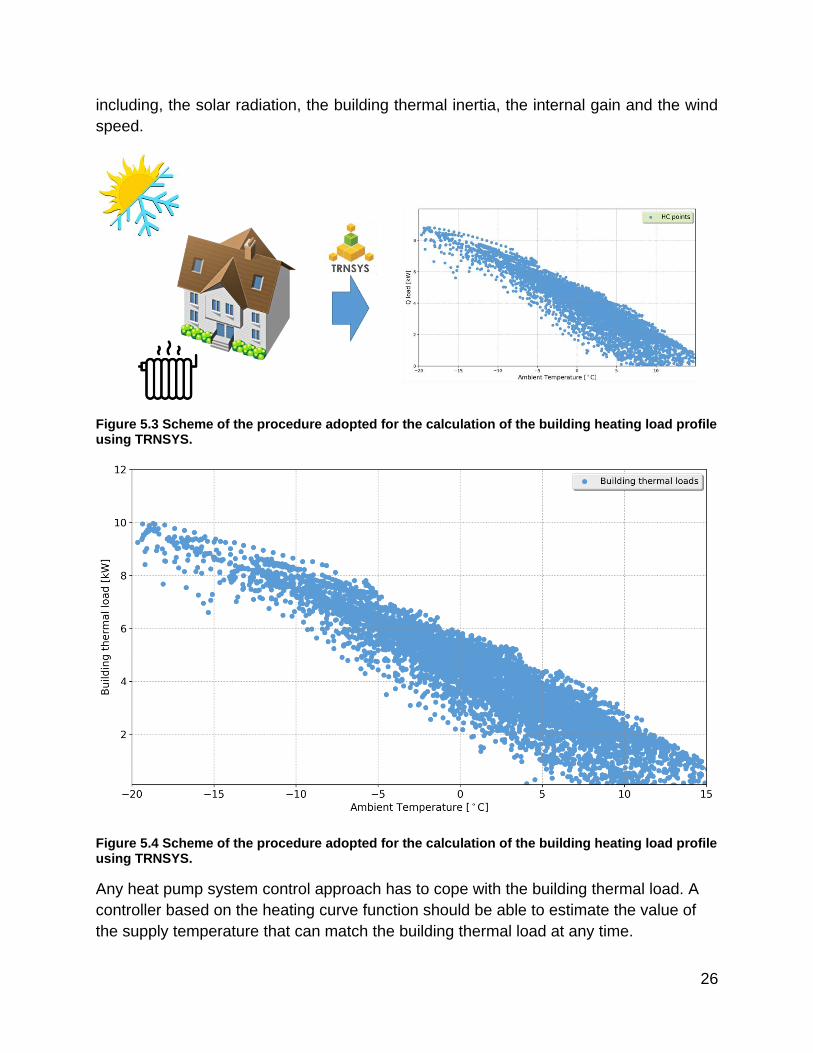
26
including, the solar radiation, the building thermal inertia, the internal gain and the wind
speed.
Figure 5.3 Scheme of the procedure adopted for the calculation of the building heating load profile using TRNSYS.
Figure 5.4 Scheme of the procedure adopted for the calculation of the building heating load profile using TRNSYS.
Any heat pump system control approach has to cope with the building thermal load. A
controller based on the heating curve function should be able to estimate the value of
the supply temperature that can match the building thermal load at any time.

27
The ideal profile of the supply temperature can be derived starting from the thermal load
profile shown in Figure 5.4 once the characteristics of the heating distribution systems
are known. Considering a radiator-based heating distribution system, the heat flow rate
of the radiator needs to match the building thermal load.
For this study, the thermal response profile of the radiator system has been calculated in
terms of total power emitted as a function of the inlet supply temperature. This calculation
has been performed again using TRNSYS and imposing a room temperature equal to
20°C. By matching the building thermal loads with the profile of the power emitted by the
radiators it is possible to calculate the supply temperature profile as a function of the
ambient temperature. The results of this procedure are shown in Figure 5.5. The Figure
that represents, in fact, the profile of the ideal supply temperature for the modelled
system.
Figure 5.5 Profile of the ideal supply temperature to the heating distribution system obtained with model simulation and example of heating curve settings.
As it can be noticed, the shape of the profile of Figure 5.5 is similar to the profile shown
in Figure 5.4. The resulting supply temperature profile appears as a cloud points with an
increasing spread at increasing ambient temperature values. The Figure also show a
typical heating curve control setting (from Figure 5.2). As it can be noticed, despite the
overall trend of the ideal supply temperatures is respected, a controller based on the
shown heating curve setting would overestimate the required supply temperature for
some values of the ambient temperature and would underestimate it for others. Intuitively,
when the supply temperature is overestimated, the energy consumption is greater than

28
required and the building tends to be overheated. On the contrary, an underestimation of
the supply temperature would lead to an indoor temperature lower than the set point.
The supply temperature values obtained from the simulation have been filtered and
analyzed in order to better investigate the influence of other input variables on the supply
temperature variation at a given ambient temperature. In particular, the study focused on
three inputs: the solar radiation, the wind speed and the internal gains.
Figure 5.6 shows the visual representation of the two subsets of data that have been
considered to define two case studies that are briefly described in the following. In both
case studies, the wind and the internal gains have been excluded from the simulations in
order to focus on the effect of the solar radiation on the supply temperature profile. The
influence of the wind and the internal gains is described in Section 5.3.
Figure 5.6 Profile of the ideal supply temperature to the heating distribution system obtained with model simulation. Case study 1: supply temperature variation for ambient temperature equal to 0.7°C. Case study 2: supply temperature variation for ambient temperature between -0.5 and 0.5°C for 24h periods with low solar radiation.
5.1 Heating curve: influence of daily solar radiation The objective of the first case study is to investigate if the required supply temperature at
a given time is influenced by the solar radiation that occurred in the previous 24 hours.
The analysis has been focused on the variation of the supply temperature for an ambient
temperature arbitrary selected equal to 0.7°C. The values considered are marked with
red crosses in Figure 5.6. The maximum, average and minimum values of the supply
temperature (S1, S2 and S3) are 42.1°C, 39.1°C and 31.9°C, respectively. The
corresponding thermal loads varies between 5.9 and 2.7 kW, with an average of 4.9 kW.

29
For each of these three values, the corresponding simulation times have been selected.
The evolution of the ambient temperature in the previous 24 hours is shown in Figure 5.7.
In Figure 5.7, T1 is the ambient temperature profile corresponding to the supply
temperature S1, T2 is the ambient temperature corresponding to S2 and T3 is the ambient
temperature corresponding to S3. The final point for all the ambient temperature profiles,
T1, T2 and T3 is the ambient temperature equal to 0.7°C. In the same Figure, the
respective daily solar radiation value profiles (DailyRad1, DailyRad2 and DailyRad3) are
reported accordingly in form of bar charts.
From the analysis of this case study it can be observed that the daily solar radiation has
a large impact on the supply temperature. In particular, the minimum supply temperature
(S3=31.9°C) is required when in the previous 24h the daily solar radiation is relatively
high (DailyRad3). On the contrary, the maximum supply temperature (S1=42.1°C) is
required when the daily solar radiation over the previous 24h is almost zero.
Figure 5.7 Case study 1: Daily solar radiation and ambient temperature profiles
5.2 Heating curve: influence of ambient temperature evolution
The second case study has been conceived as a counterpart of the first case study. The
objective is to investigate if the required supply temperature at a given time is influenced
by the ambient temperature evolution over the previous 24 hours, considering days where
the solar radiation is relatively low. For this purpose, the data from the simulation results
has been filtered in order to select the supply temperature required when the daily solar

30
radiation has been lower than an arbitrary threshold of 1500 kWh/m2 and the ambient
temperature was between -0.5 and +0.5 °C over the previous 24h. The idea is here to
explain the variation of the required supply temperature for a given ambient temperature
during days with almost no solar radiation.
Figure 5.8 Case study 2: Daily solar radiation and ambient temperature profiles
The resulting thermal loads varies between 5.9 and 5.0 kW, with an average of 5.5 kW.
The maximum, average and minimum values of the supply temperature (S1, S2 and S3)
are 42.2°C, 40.8°C and 39.4°C, respectively. For each of these three values, the
corresponding simulation times have been selected and the respective evolution of the
previous 24 hours is shown in Figure 5.8. In the Figure, T1 is the ambient temperature
profile corresponding to the supply temperature S1, T2 is the ambient temperature
corresponding to S2 and T3 is the ambient temperature corresponding to S3. In the same
Figure, the respective daily solar radiation value profiles (DailyRad1, DailyRad2 and
DailyRad3) are reported accordingly in form of bar charts.
From the analysis of the second case study it can be observed that in days with low daily
solar radiation, the persistence of the ambient temperature has an influence on the supply
temperature. In particular, the minimum supply temperature (S3=39.4°C) is required
when in the previous 24h the ambient temperature (T3) is higher than the final value. On
the contrary, the maximum supply temperature (S1=42.2°C) is required when the ambient
temperature (T1) over the previous 24h occurred to be always lower than the final value.

31
It is worth to observe that the influence of the temperature persistence on the required
supply temperature is much lower than the effect of the daily solar radiation.
5.3 Heating curve: influence of solar radiation, wind and internal gains
An approach similar to the one adopted in Sections 5.1 and 5.2 has been used to compare
the influence of solar radiation, the wind speed and the internal gains on the required
supply temperature.
The model used to obtain the results shown in Figure 5.5 has been used to perform
simulations where one input among solar radiation, wind speed and the internal gains has
been selectively excluded from the model. In particular, the simulation has been
performed once excluding only the solar radiation from the model and maintain all the
other inputs (wind and internal gains). Another run has been performed selectively
excluding the wind input and, finally, a further simulation has been run excluding the
internal gains. The simulation results obtained with this approach have been used to
evaluate qualitatively and quantitatively the supply temperature variation at given ambient
temperatures.
For the sake of explanation, a subset of the obtained results are given in Figure 5.9 where
35 values have been randomly chosen from the supply temperature profile (Figure 5.5)
in order to cover the range of ambient temperature between -20 and +15 °C. From the
qualitative point of view, the results show the variation of the calculated building thermal
loads obtained by the selective exclusion of solar radiation, wind and internal gains from
the model.
To make the qualitative comparison more clear, in Figure 5.10, 5.11 and 5.12 show the
comparison of the supply temperature variations resulting from each selective simulation.
In particular, Figure 5.10 shows the qualitative comparison of the supply temperature
profile when the solar radiation input has been excluded from the model input. In order to
give a comparison reference, the same Figure shows also the heating curve setting from
Figure 5.2. Similarly, Figure 5.11 and Figure 5.12 propose the same comparison
approach when the wind velocity and the internal gains, respectively, have been
excluded. The inspection of the Figures reveals that the exclusion of the solar radiation
from the simulation inputs has a relatively high impact on the required supply temperature.
Also, this effect appears to be greater for higher ambient temperature values. Secondly,
the required supply temperature variations obtained excluding the internal gain input
show a relatively smaller and more uniform displacement over the entire ambient
temperature range. Finally, the effect of the wind on the required supply temperature
appears to be less significant.

32
Figure 5.9 Example of variation of the required supply temperature values obtained by simulations where solar radiation, wind, and internal gains inputs have been selectively excluded from the model.
Figure 5.10 Comparison between the ideal required supply temperature and the values obtained by simulations where the solar radiation input has been excluded from the model.

33
Figure 5.11 Comparison between the ideal required supply temperature and the values obtained by simulations where the wind input has been excluded from the model.
Figure 5.12 Comparison between the ideal required supply temperature and the values obtained by simulations where the internal gain input has been excluded from the model.

34
From the quantitative point of view, Figure 5.13, 5.14 and 5.15 show a box plot
representation for the differences of the required supply temperature over the ambient
temperature range divided in 5°C ranges. Figure 5.13 shows that the excluding the solar
radiation input from the model inputs has a relatively low impact for low ambient
temperature values. On the other hand, the influence is much more relevant for ambient
temperatures between 0 and 15°C. When the ambient temperature is between 10 and
15°C the median value of the difference (red line in the box plots) is about 5 degrees.
Similarly, Figure 5.14 shows the difference calculated considering the supply temperature
obtained when the wind velocity has been excluded from the model input. The difference
distribution does not show relevant differences over the ambient temperature range, even
if a slight increase can be observed for ambient temperatures greater than 5°C. The
median value of the calculated difference is always lower than 1°C.
The evaluation of the influence given by the internal gain input is shown in Figure Figure
5.15. In this case the median value of the calculated difference is always lower than 2°C.
The percentage variations resulting from the annual simulations have been calculated considering the entire ambient temperature range between -20 and 15°C and the summary of the results is shown in Figure 5.16.
Figure 5.16 summarizes the quantitative analysis showing the required supply
temperature difference depending on each considered input. As already clear from the
qualitative analysis, the solar radiation is the input the contribute the most to the variation
of the building thermal loads at given ambient temperature. On the other hand, the thermal
load variations due to the internal gains is secondary and, finally, the wind speed results
to play the least significant role.
Figure 5.13 Variation of the required supply temperature when the solar radiation input is excluded.

35
Figure 5.14 Variation of the required supply temperature when the wind velocity input is excluded.
Figure 5.15 Variation of the required supply temperature when the internal gain input is excluded.
Figure 5.16 Percentage variation of the required supply temperature when internal gains, solar radiation and wind speed are selectively excluded.

36
5.4 Modelling of building packages The final stage of the modelling work presented in this Chapter consisted in the
development of simulation models with reference to different building envelopes and
different heating distribution systems.
The reference parameters for the building envelopes have been derived from Tabula [51].
Also, the building models have been modified in order to be consistent with the building
energy classification provided by the Boverket [52] (Swedish National Board of Housing,
Building and Planning). As a results, the building packages have been modelled as shown
in Table 5.1.
Table 5.1. Building package models developed.
Boverket class Heating distribution system
A Floor heating
B Floor heating
B Radiators
D Radiators
Figure 5.17 Building thermal load profiles of the model packages developed with reference to the Tabula [51] database and the Swedish building classification criteria provided by Boverket [52].

37
Figure 5.17 shows the building thermal load profiles related to the modelled building
packages. The profiles have been obtained following the approach described in this
Chapter. Worth noticing, the axis ranges are the same in every sub-Figure. The Class D
package can be considered as a model of a relatively old building constructed in Sweden
in the 1960s and equipped with radiators, according to the references provided by the
Tabula database [51]. Two Class B packages have been modelled; One package
considers a standard envelope where a common radiator system is installed. The second
Class B package considers the characteristics of an envelope refurbished for a floor
heating system. In general, it can be observed that, compared to the Class D package,
the Class B buildings have lower thermal load values, especially for low ambient
temperatures. Finally, the Class A package considers a low-energy building with the
characteristics of a modern construction.
From all the profiles shown in Figure 5.17 it can be clearly observed a variation of the
thermal loads for given values of the ambient temperature. As already mentioned in this
Chapter, the variation tends to be larger for higher values of the ambient temperature,
suggesting that, for all these buildings, the thermal loads are influenced by other variables
that are not considered in the conventional control approach.
5.5 Final remarks This Chapter addressed the evaluating of the influence of several variables on the
required supply temperature that a heat pump controller needs to provide in order to allow
the heating system to correctly cope with the building thermal loads.
The study investigated in particular the influence of the solar radiation, wind velocity and
internal gains on the required supply temperature.
The results show that the solar radiation has a large impact on the building thermal loads
and the required supply temperature especially for ambient temperatures between 0 and
15°C. This influence is not accounted in the conventional control implementation.
In general, potential improvements of the heating curve approach are possible. A control
algorithm for the adaptive modulation of the heating curve (supply temperature)
depending on additional inputs can potentially lead to operate the system more efficiently,
prevent the overheating or underheating of the building and decrease the system energy
consumption.
An improvement potential study has been performed to show the potential improvement
of the performance in a heat pump system where the heating curve control is
implemented. The implementation and results are described in Chapter 6.

38
5.6 Publication (WP5) On this topic, a scientific paper will be submitted to Energy and Buildings by summer 2018
with the title “On the improvement of conventional methods to control residential heat
pump systems. Part I: the influential parameters on the demand side” (Rolando D. and H.
Madani)

39
6 Improvement potential study (WP3)
6.1 Research questions Given the results obtained from the study described in Chapter 5, a study has been
dedicated to investigate the energy saving potential that can be obtained with the
improvement of the heating curve control approach considering the perfect prediction of
the solar radiation, the ambient temperature and the internal gains. In this study, the
perfect prediction of the Domestic Hot Water consumption has also been considered.
The purpose of the study is the evaluation of the improvement potential of a heat pump
heating system with the control logic based on the heating curve approach.
6.2 Improvement potential: implementation A TRNSYS dynamic model has been developed considering a single family house
heating system sited in Stockholm. The system layout adopted in this study has been
already described in Section 4.4 and includes the simulation sub-models of Borehole Heat
Exchanger (BHE), Ground Source Heat Pump (GSHP), storage tank building, circulation
pumps and auxiliary heater.
The Heat Pump considered is a ground-source single speed unit modeled by means of a
performance map as explained in Section 4.1. The compressor electrical power and
condenser heat transfer rate have been derived as a function of the approaching heat
source temperature to the evaporator (brine side) and approaching heat sink temperature
to the condenser (water side), respectively named source temperature (Tsource) and load
temperature (Tload). The heat pump model has been sized in order to obtain a heat
capacity equal to the building heat demand (balance point) when the ambient temperature
is about -4°C.
The ground heat exchanger is implemented by means of a short-term ground response
model based on a borehole thermal resistance and capacitance approach.
The storage tank is connected on the heating generation side to the heat pump condenser
and on the heating distribution side to the hydronic loops for both Domestic Hot Water
(DHW) and Space Heating (SH). It is modeled as a 300 l stratified cylindrical tank with 10
virtual isothermal volume nodes. Both hydronic loop connections are modeled through
three ports. On the heating distribution side, the virtual top node is connected to the
domestic hot water, the middle node is connected to the space heating and the bottom
node is connected to the return water flow. On both heat pump and heating distribution

40
sides, the inlet node is dynamically chosen according to the inlet water temperature in
order to preserve the temperature stratification.
Two coiled heat exchangers are modeled inside the storage tank, one in the virtual top
node for DHW and one in the middle node for SH. Both heat exchangers are connected
to an auxiliary heater operating when the heat pump is not sufficient to fulfill the DHW or
space heating demand. For DHW operation mode, the auxiliary heater has a heating
capacity of 5 kW while for the SH mode the auxiliary heater can operate at three different
stages delivering a power of 3, 6 or 9 kW.
The building dynamic sub-model considers a single zone with reference to the
characteristics and information provided by the Tabula web tool [51] for a standard
Swedish residential building. A single family house located in Stockholm (Sweden) and
built between year 1996 and 2000. The glazing surfaces represent the 33% of the wall
surface and the 18% of the total envelope including the roof surface.
For the given building model characteristic, a building heating curve is defined in order to
calculate the required supply temperature of the space heating distribution system.
The space heating distribution system consists of radiators and pipings and it is
modeled through the TRNSYS Type 362. The middle port of the thermal storage tank
supplies the radiator and the return flow enters the thermal storage tank at the node with
the closest temperature. A tempering valve coupled with a mixing valve is included in the
system at the radiator loop return in order to keep the radiator supply temperature close
to the required temperature (𝑇𝑠𝑢𝑝𝑝𝑙𝑦𝑟 ). A Proportional Integrative controller (PI) has also
been implemented and tuned to control the mass flow rate of the radiator and maintain
the supply temperature as close as possible to the set point given by the heating curve
(𝑇𝑠𝑢𝑝𝑝𝑙𝑦𝑟 ).
Two different operating modes are defined for the heat pump system controller. In the
DHW mode the on-off controller operates according to a constant hysteresis logic and it
is set to maintain the storage tank top node temperature not lower than 42.5°C. The heat
pump is turned on when the storage tank temperature is lower than 42.5°C and it is turned
off when the tank temperature reaches the value of 47.5°C. The auxiliary heater is turned
on providing a heating power of 5 kW when the storage tank temperature of the top node
is lower than 42.5℃ for more than 20 minutes and it is turned off when the temperature
reaches the value of 45°C.
In the SH mode the controller logic is based on a degree-minute parameter (DM)
defined in Eq. 7 [4].
𝐷𝑀 = (𝑇𝑠𝑢𝑝𝑝𝑙𝑦 − 𝑇𝑠𝑢𝑝𝑝𝑙𝑦𝑟 ) ∙ 𝑡 + 𝐷𝑀𝑜𝑙𝑑 (7)

41
Where 𝑇𝑠𝑢𝑝𝑝𝑙𝑦 is the actual space heating supply temperature, 𝑇𝑠𝑢𝑝𝑝𝑙𝑦𝑟 is the supply
temperature given by the building heating curve, t is the time expressed in minutes and
𝐷𝑀𝑜𝑙𝑑 is the previous degree-minute value.
According to the algorithm implemented in the system controller the heat pump is
turned on when DM is lower than -60 degree-minute and it is turned off when DM reaches
0 degree-minute.
The degree-minute value is reset to zero when the difference between the actual and
the required supply temperature values are greater the 10°C or the degree-minute value
is higher than 300. The first, second and third stages of the auxiliary heater (3kW, 6kW,
9kW) are turned on when DM is lower than -600, -680 and -760 degree-minute
respectively. The logic for turning off the space heating auxiliary heater is based on the
temperature difference. The third, second, and first stages are turned off when the
difference between the actual and the required supply temperatures is higher than 1K, 2K
and 3K respectively.
Among the simple on-off control techniques the degree-minute control logic has been
demonstrated to guarantee the lowest annual energy usage of both compressor and
electric auxiliary heater and the highest seasonal performance factor compared to
constant or floating hysteresis methods [4].
The improved potential study has been carried out in order to evaluate the possible
enhancements of the heating system described above considering new control strategies
based on additional input information. Auxiliary variables have been added to the system
controller including the forecast of DHW consumption, internal gain, ambient temperature
and solar radiation. For this study, the developed control logics described below are
based on the assumption of perfect prediction for the forecasted data.
6.3 Results The results are here summarized and discussed with reference to the basic on-off
control logic based on the degree-minute approach described in Section 6.2.
For all the simulations, in order to discuss the results in term of indoor temperature
stability, a dedicated parameter has been defined with respect to a temperature dead-
band of ±0.5°C for the room temperature. The parameter takes into account the duration
and the magnitude of the deviation from the dead-band limits and can be specified for
both space heating and domestic hot water modes.
The discretized expressions of the temperature dead-band deviation (DBD) parameter
is shown in Eq. 8 and 9.

42
DBDSH = ∑ {〖(𝑇〗low, i
SH − 𝑇actual, iSH ) ∙ (𝑡𝑖 − 𝑡𝑖−1), if 𝑇actual, i
SH < 𝑇low, iSH
〖(𝑇〗actual, iSH − 𝑇high, i
SH ) ∙ (𝑡𝑖 − 𝑡𝑖−1), if 𝑇actual, iSH > 𝑇high, i
SH
𝑛
𝑖=0
(8)
DBDDHW = ∑(𝑇low, iDHW − 𝑇actual, i
DHW ) ∙ (𝑡𝑖 − 𝑡𝑖−1), if 𝑇actual, iDHW
𝑛
𝑖=0
< 𝑇low, iDHW (9)
Where 𝑛 is the amount of minutes included in the analyzed period, t is the time
expressed in minutes, 𝑇lowSH and 𝑇high
SH are respectively the lower and higher dead-band
limits. 𝑇lowDHW is the DHW comfort limit arbitrarily fixed to 42.5℃ while 𝑇actual
SH and 𝑇actualDHW are
respectively the space heating and the DHW actual values.
6.3.1 Domestic hot water consumption perfect prediction
A DHW consumption profile based on a stochastic bottom-up model [53] has been
adopted and specified for a residential building with 2 adults and 2 children.
The improved logic has been developed calculating a dynamic draw-off schedule
considering the forecasted DHW profile. The purpose of this approach is to develop an
improved control logic based on the idea of running the system reducing the electrical
energy consumption. The dynamic schedule approach considers the amount of energy
required by the draw-offs and it is therefore based on dynamic anticipation of the energy
request. In particular, the required running time of the heat pump is anticipated by
computing the ratio between the future energy demand and the expected condenser heat
rate based on an average of the condenser power. For each draw-off, the anticipation
time is evaluated as the running time required by the Heat Pump to provide the related
amount of energy.
In the controller, the dynamic schedule signal is combined with the on-off hysteresis
signal. The heating system operation mode is selected depending on the thermal storage
tank temperature at the virtual top node. Worth mentioning, the implemented control logic
always prioritizes the DHW demand over the space heating.
In Figure 6.1 an example of the results obtained from the simulations considering the
month of August. The Figure shows the profiles of the DHW tank top node obtained by
the base control and by the control that exploit the perfect prediction of the DHW
consumption. For the proposed control, a higher stability of the temperature can be
observed within the indicated set point dead-band. Considering the summer season, the
developed control logic for the DHW consumption described in Section 6.3.1 allows an
improvement in the water temperature profile stability together with an overall potential
energy saving of about 6%. The dead-band deviation obtained with the improved logic is

43
0.5% less than the DBD value obtained by the original control. The usage of the auxiliary
heater is also drastically decreased over the summer season by more than 93%.
Figure 6.1 Profiles of the top node temperature of the DHW tank obtained with the basic and improved controls. The example shown is related to the simulation results over the month of August.
6.3.2 Internal gain perfect prediction
A stochastic occupancy profile model [54] combined with metabolic rate and domestic
lighting power gains have been adopted in order to calculate an internal gain profile
consistent with the single family house application considered in this study.
Similarly, to the approach adopted for the DHW consumption control logic, an
anticipation schedule has been calculated based on the perfect prediction of the internal
gain profile forecast. The anticipation period adopted is fixed to one hour. In order to
investigate the impact of the internal gain on the room temperature and the energy saving
potential, the monthly solar radiation has been considered constant to the average value
of each month.
The approach adopted is based on the modulation of the building heating curve by
introducing a linear offset correction to the required supply temperature (𝑇𝑠𝑢𝑝𝑝𝑙𝑦𝑟 ) based
on the internal gain profile. A distinction has been made in order to define different
operation modes, one focusing on the thermal comfort condition stability (“comfort mode”)
and one focusing on the maximization of the energy saving (“economy mode”).

44
Figure 6.2 Internal gain perfect prediction: comparison between the basic and the improved control logic with reference to (a) the indoor temperature and (b) the supply heating temperature
For the internal gain improvement potential study, the months of January and March
have been considered as test periods. Figure 6.2 shows the results of the comparison
between the basic and the improved logic over a 24h period selected in the simulation
month of March. As can be observed in Figure 6.2a, the indoor temperature obtained by
the basic controller is affected by the given internal gain profile and the potential for indoor
overheating due to the internal gains can be identified and avoided. On the other hand,
the improved control logic allows to better maintain the indoor temperature within the
reference dead band of 21±0.5°C. Figure 6.2b shows the corresponding results in terms
of supply heating water temperature over the same 24h period where the improved logic
is able to reduce the overheating effect and consequently reduce the the electricity use
of the system by adjusting the building heating curve.
6.3.3 Solar radiation perfect prediction
A procedure for the heating curve modulation based on the perfect prediction of the
solar radiation profile has been also implemented to investigate the energy saving
potential that can be obtained.
The aim of the developed control logic is to avoid the possible building overheating
maintaining a more stable room temperature close to the set point value.
The solar radiation profile has been provided by the Meteonorm database [55]. A set
of 4 corrective coefficients have been employed to adjust the heating curve accounting
for the energy gain by considering both the instantaneous and predicted total radiation.
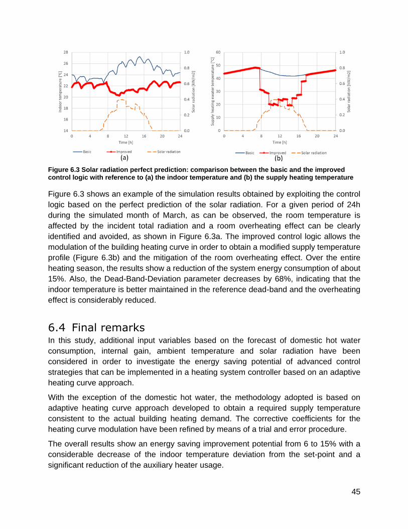
45
Figure 6.3 Solar radiation perfect prediction: comparison between the basic and the improved control logic with reference to (a) the indoor temperature and (b) the supply heating temperature
Figure 6.3 shows an example of the simulation results obtained by exploiting the control
logic based on the perfect prediction of the solar radiation. For a given period of 24h
during the simulated month of March, as can be observed, the room temperature is
affected by the incident total radiation and a room overheating effect can be clearly
identified and avoided, as shown in Figure 6.3a. The improved control logic allows the
modulation of the building heating curve in order to obtain a modified supply temperature
profile (Figure 6.3b) and the mitigation of the room overheating effect. Over the entire
heating season, the results show a reduction of the system energy consumption of about
15%. Also, the Dead-Band-Deviation parameter decreases by 68%, indicating that the
indoor temperature is better maintained in the reference dead-band and the overheating
effect is considerably reduced.
6.4 Final remarks In this study, additional input variables based on the forecast of domestic hot water
consumption, internal gain, ambient temperature and solar radiation have been
considered in order to investigate the energy saving potential of advanced control
strategies that can be implemented in a heating system controller based on an adaptive
heating curve approach.
With the exception of the domestic hot water, the methodology adopted is based on
adaptive heating curve approach developed to obtain a required supply temperature
consistent to the actual building heating demand. The corrective coefficients for the
heating curve modulation have been refined by means of a trial and error procedure.
The overall results show an energy saving improvement potential from 6 to 15% with a
considerable decrease of the indoor temperature deviation from the set-point and a
significant reduction of the auxiliary heater usage.

46
In particular, in the studied system, the perfect prediction of the Domestic Hot Water
consumption could lead to a potentially energy saving of about 6%. The perfect prediction
of the internal gain profile can allow an annual energy saving up to 7%. The most
promising result has been obtained considering the perfect prediction of the solar
radiation at 1-hour horizon, with an energy saving potential of about 15%.
6.5 Publications (WP5) The results of the improvement potential study described in this Chapter have been
published at the 12th IEA Heat Pump Conference that has been held in Rotterdam in
2017. The title of the paper is “Heat pump system control: the potential improvement
based on perfect prediction of weather forecast and user occupancy” [56] and it has been
presented as an oral presentation during the Conference.
A Master Thesis has been also developed on this topic by Roberto Tomasetig and
Giacomo Braida with the title “Preliminary analysis of the potential energy saving
achievable with a predictive control strategy for a single family house heat pump system”
[65]

47
7 Weather data for system control (WP3)
7.1 Research questions In the study carried out in Chapter 6 the perfect prediction of a number of variables
regarding weather condition has been considered. In order to move beyond the perfect
prediction assumption, a further investigation has been carried out in order to evaluate
the possibility to integrate the information from weather services into an adaptive heating
curve control.
The data from a number of different weather sources has been collected and analyzed
focusing on selected services available for Swedish cities. The reliability of the weather
forecast has been evaluated with reference to 8 Swedish cities. Application Program
Interfaces (APIs) have been developed to allow the weather data measurements and
forecast to be easily implemented in heating system controllers including heat pumps
units.
7.2 City selection A selection of the main locations to be considered when collecting the required data has
been performed. Eight different cities have been selected and they are shown in Figure
7.1.
The selection of these cities has two main reasons. First, the cities have been selected in
order to cover the four climate zones defined in Sweden [52]. Secondly, the selection
criteria aimed to include both big cities (like Stockholm and Gothenburg) and small cities
(like Törsby).
7.3 Weather data sources A selection of the different weather sources that are used to collect all the instantaneous
and forecast data is necessary. Figure 7.2 shows the logos of the selected weather
sources.

48
Figure 7.1. Cities map with indication of Swedish Climate Zone. Source: Boverket’s building
regulations, 2016.
With the idea of carrying an analysis on weather services available in Sweden, the first
source to be selected is the one related to the Swedish Meteorological and Hydrological
Institute (SMHI) [57], being one of the most famous weather forecasts service in Sweden.
SMHI is an agency under the Swedish Ministry of the Environment and Energy. The
service utilises collected observational data which is processed by models and
meteorologists. In order to predict weather, numerical forecast models are used.
Figure 7.2 Weather services used in this project.
The second source selected is the Norwegian weather service YR.no (YR) [58] that offers
an online weather service that is the 5th most visited weather service on the internet.
YR web application offers forecasts for more than 9 million places in the world. The
forecasts are based on data from the Norwegian Meteorological Institute and several
international meteorological organisations (like ECMWF and EUMETSAT).

49
The American weather service Weather Underground (WUND) [59] is a commercial
weather service providing real-time weather information via Internet. WUND provides
weather reports for most major cities across the world on its website, as well as local
weather reports for newspapers and websites. Its information comes from the National
Weather Service (NWS), and from members with automated personal weather stations
(PWS); currently, Weather Underground uses observations from over 250,000 personal
weather stations worldwide.
OpenWeatherMap (OWM) [60] is an online service that provides weather data, including
current weather data, forecasts, and historical data. For data sources, it utilizes
meteorological broadcast services, raw data from airport weather stations, raw data from
radar stations, and raw data from other official weather stations. All data is processed by
OpenWeatherMap in a way that it attempts to provide accurate online weather forecast
data and weather maps.
Finally, SLB-analys (Stockholm Air and Noise Analysis) [61] has been considered in this
study. This service is a department at the Environment in Stockholm, which is
responsible for monitoring air environment of the city. Also, it provides a regional system
for air surveillance on behalf of the East Sweden Air Pollution Control Association. Along
with all these activities, the official website also provides real-time weather data gathered
from 4 different stations located in Stockholm: Södermalm, Högdalen, Marsta and
Malma. SLB does not provide weather forecast data.
Table 7.1 shows the updating time intervals of the real time measurements for each
weather services while Table 7.2 shows the updating interval for weather forecast
information.
Table 7.1. Updating time interval for real time measurements provided by the four different weather sources selected.
OWM SLB SMHI WUND
Instantaneous
Measurements 30 min 1 h 1 h < 20 min
Table 7.2. . Updating time interval for forecasts provided by the four different weather sources selected.
OWM YR SMHI WUND
Forecasts 3 h 1 h 1 h 1 h

50
7.4 Application Program Interface (API) development The study has been developed along different stages where the weather data from the
mentioned cities and sources have been collected and analysed. The access to the
weather sources required the implementation of dedicated computer code and the design
and development of a suitable database structure. Some of the considered weather
sources provides APIs for accessing weather measurements and forecast (OWM,
WUND, SMHI) while other sources don’t provide native interfaces (SLB, YR). A dedicated
SQL database has been designed to collect the data and server side auxiliary APIs have
been developed in PHP in order to manage the data collection in the database. When
used in the context of web development, an API is typically defined as a set of Hypertext
Transfer Protocol (HTTP) request messages, along with a definition of the structure of
response messages, which is usually in an Extensible Markup Language (XML) or
JavaScript Object Notation (JSON) format.
Particularly, in the presented work it has been decided to work with structure of response
message in JavaScript Object Notation, that is a language-independent open-standard
data format, using human-readable text to transmit data objects consisting of attribute–
value pairs and array data types (or any other serializable value).
Due to its simplicity and a design philosophy that emphasizes readability, nowadays many
programming languages include code to generate and parse JSON-format data. Having
a universal JSON-format for output data, the developed APIs could become a possible
product easily exploitable by the project partners. In Figure 7.3 it is reported a typical
example of JSON-format output data for weather forecasts.
For the client side access to the collected data, both Python and web interfaces have
been developed.
Figure 7.3 Example of JSON-format for weather forecast information from API.
Worth noticing, not all the selected weather sources had an already developed API for
both instantaneous and forecast weather data collection. For SLB and YR, an additional

51
work has been dedicated to the implementation of scripts able to collect the available data
from the respective web applications.
7.5 Results and remarks In this Chapter examples of sources for weather forecast and the uncertainties associated
to the data have been presented. Different forecast horizons have been compared
considering different cities and different weather variables. In particular, the weather
variables accounted in the accuracy analysis are the ambient temperature, the wind
speed, the solar radiation and the cloudiness index. Not all these variables are available
from all the considered weather sources and Table 7.3 shows the availability summary.
Table 7.3. Availability of weather variable subset considered in the study.
OWM SLB [1] SMHI WUND
Temperature [°C]
Wind speed [m/s]
Solar Radiation [W/m2]
Cloudiness [%]
For sake of brevity only a short summary of the results and comparison is here included.
The complete analysis can be found in the Publication indicated in Section 7.6.
The weather data has been collected over the period from October 2017 to March 2018.
Figure 7.4 shows an example of the obtained results. In the Figure, the distribution of the
percentage errors of the forecast for the ambient temperature is reported considering a
3-hour horizon. The median value of the forecast errors (the white dot of the violin plots
[62]) is similar for all the weather sources and the cities considered. Worth noticing, the
temperature forecast for small cities (Törsby and Umeå) contains more outlier values
compare to big cities like Stockholm or Gothenburg. However, this observation cannot
lead to generalized conclusions.
The implementation of APIs for weather data management have been briefly described.
The API developed in the Project can be easily integrated to heat pump control in order
to implement adaptive heating curve solutions.
[1 ] values available only for Stockholm

52
It is worth noticing that no weather service able to provide forecast of the solar radiation
could be found. Also, only few weather services include the solar radiation measurements
in their APIs and less than 15% of the available weather stations are instrumented to
measure the solar radiation. On the other hand, as already discussed in Chapter 5 and
6, the energy gain due to the daily solar radiation can play an important role in the control
of a heating system. For these reasons, an approach for the prediction of the daily solar
radiation that can be employed for the system control purposes is proposed in Chapter 8.
Figure 7.4 Temperature forecasts errors based on the analysis performed on forecasts at 3h horizont over the period from October 2017 to March 2018.
7.6 Publication (WP5) More details about the analysis carried out on the weather data can be found in the Master
Thesis that has been developed and published on this topic by Mattia Monteggia, from
Politecnico di Milano, a guest Master Thesis Student at KTH Energy Technology
Department. The title of the thesis is “Weather data for heat pump system control
improvement: analysis of instantaneous and forecasted measurements and evaluation of
potential energy savings” [66].

53
8 Heating curve adjustment with daily solar radiation prediction model (WP3)
8.1 Introduction The analysis of the weather data carried out in Chapter 7 has been used as a starting point for the design and development of an innovative control for heat pump systems based on the prediction of the solar radiation energy gain.
In this Chapter the description of the proposed control approach is provided and examples of the results that can be obtained in terms of annual reduction of energy consumption are presented.
8.2 Weather data overview: Stockholm annual profiles Figure 8.1 shows the monthly distribution of the ambient temperature in Stockholm
considering the measurements provided by the weather service SLB [61] over the period
2014-2017. A few things can be observed from the inspection of the Figure. As expected,
the winter months December, January, February and March present the lowest peaks.
On the other hand, the violin plot representation [62] here proposed reveals for example
that the median value (white dot) of the ambient temperature measured in December is
similar to the median obtained in October. Also, the median value calculated in November
is similar to the value calculated in April.
Figure 8.2 shows the distribution of the daily solar radiation over the same period (2014-
2017). In this case, a remarkable difference can be observed between November or
December and March or April, respectively. Intuitively, this is of course due to the fact
that (in Stockholm) during March and April the daylight time is much longer than in
November and December and, in general, a higher number of sunny days are present.
A heat pump control based on the heating curve approach rely on the calculation of the
required supply temperature based on the ambient temperature value. On the other hand,
the observations derived from both Figure 8.1 and Figure 8.2 imply that, without
accounting for the solar radiation gains, the same value of supply temperature can be
calculated, for example, in November and April.
The study proposed in Chapter 5 and the improvement potential analysis described in
Chapter 6 show that the prediction of the solar radiation can be effectively used to improve
the heating curve controller typically implemented in heat pump units. As a result, an
improvement of the system can be expected in terms of energy saving and indoor
conditions.

54
Figure 8.1 Monthly ambient temperature distribution in Stockholm over the period 2014-2017,
according to the SLB-analys database [61].
Figure 8.2 Monthly values of the daily solar radiation distribution in Stockholm over the period
2014-2017, according to the SLB-analys database [61].

55
8.2.1 Overview of weather variables over one-month
In the Project, a study has been dedicated to the possibility of indirectly predict the daily
solar radiation.
Figure 8.3 shows the profiles of a number of weather variables that have been taking into
account to design the prediction model described in the following Section. The data
shown in the Figure is referred to the measurements May 2014 in Stockholm and retrieved
from the SLB database [61]. In particular, the Figure 8.3a shows the daily values of solar
radiation, Figure 8.3b the ambient temperature, Figure 8.3b the cloudiness index and
Figure 8.3d the relative humidity. In Figure 8.3b the ambient temperature daily profile
includes the average values (dots) and the variation range.
The Figure is proposed to qualitatively show that a correlation between the cloudiness
index and the solar radiation can be observed. Considering for example the five days
around day 130 (indicated in Figure 8.3a, 8.3b and 8.3c with an arrow) it can be observed
that days with a relatively low daily solar radiation value (lower than 2000 kWh/m2)
typically corresponds to days where the cloudiness index is relatively high (above 60%).
A similar observation can be made comparing the relative humidity profile (Figure 8.3d)
and the solar radiation profile (Figure 8.3a).
Figure 8.3 Overview of the weather measurements over one month period (Stockholm, May 2014, SLB database [61]).

56
From these observations, a model for the solar radiation prediction has been developed
with the purpose of providing a tool for the estimation of the daily solar radiation that can
be employed to adjust the heating curve and improve the heat pump system control.
8.3 Daily solar radiation prediction: model development The basic idea of the prediction model here presented rely on the possibility to evaluate
the expected “maximum” value of the horizontal solar radiation for any given point on the
earth surface at a given time. In fact, as discussed in [63], [64], the so called clear-sky
radiation can be evaluated by calculating, at a given time, the relative position of the sun
to a given geographical location.
This calculation can be implemented in a computer code in order to evaluate the clear-
sky radiation having as input the latitude, the longitude and the time. An illustrative
scheme of the procedure is shown in Figure 8.4. The Python PySolar library [65]
implements the models and algorithms developed in [63], [64] and easily allow to perform
the evaluation of the clear-sky radiation.
An example of the results that can be achieved is proposed in Figure 8.5. The Figure
shows the profile of the clear-sky radiation for an arbitrary selected day. Also, the same
Figure includes the corresponding profile of the measured total horizontal radiation from
the weather service SLB [61].
Figure 8.4 Scheme of clear-sky radiation evaluation principle. At any given time the clear-sky radiation value depends only on geographical data and geometrical calculations.

57
Figure 8.5 Example of one day profile of clear sky radiation, calculated by means of the PySolar library [64], and the corresponding measured radiation obtained from the SLB-analys database [61]
Figure 8.6 Profile of the monthly irradiance ratio calculated considering the clear sky radiation and the measurement of the solar radiation for Stockholm over the period 2014-2017.

58
As it can be clearly observed in Figure 8.5, the measured values of the solar radiation are
lower than the corresponding values of the clear-sky radiation. This reduction is due to a
number of factors including, among others, the cloudiness index, the relative humidity.
The irradiance ratio can be defined as the ratio between the actual solar radiation
measurement and the corresponding clear-sky radiation. Considering the reduction
observed in Figure 8.5, the monthly distribution of the irradiance ratio for Stockholm
between 2014 and 2017 is shown in Figure 8.6. As it can be noticed, the maximum value
of the irradiance ratio is about 0.8. This implies that the solar radiation in the considered
measurements is never greater than 80% of the clear-sky radiation values. For the
purpose of this study it is worth to mention that the months of March, April, May, and
September present an irradiance ratio between 0.3 and 0.7. This observation is relevant
for the definition of the estimation method that is described in the following Section.
8.3.1 Estimation of the daily solar radiation
The proposed method for the prediction of the daily solar radiation is based on the estimation of the irradiance ratio following on the forecast of the cloudiness index.
First, the clear-sky radiation has to be calculated for the location and the period of interest. Worth noticing, the clear-sky radiation annual profile for a given location can be considered the same for any year, since the difference in the relative position of the sun from one year to another is negligible. The daily solar radiation can then be easily calculated by simple integration of the solar radiation values over 24h.
Next, the estimated daily radiation can be calculated by means of Table 8.1. In the Table,
three reduction classes are defined depending on three ranges of the forecasted value
for the cloudiness index. Considering the forecasted cloudiness index over the daylight
period, the values of the estimated solar radiation can be calculated multiplying the clear-
sky radiation by the irradiance ratio provided in the Table. Finally, the estimated value of
the daily solar radiation can be calculated by integration over 24h.
Table 8.1. Defined ranges for the estimation of the irradiance ratio based on the cloudiness index.
Cloudiness index range [%] Irradiance ratio Reduction class
0 - 20 0.1 1
20 - 70 0.35 2
70 - 100 0.8 3
8.3.2 Heating curve adjustment with daily solar radiation prediction
Once the predicted daily solar radiation values are available, a modulation of the heating
curve function can be implemented in order to allow the controller to estimate the required

59
supply temperature to the heating distribution system by accounting not only the ambient
temperature.
The heating curve modulation proposed is based on the following empirical expression:
T_supplyrequired = T_supplyheating curve − 𝑐1 ∙Predicted daily Solar radiation
𝑐2 (10)
Where c1 and c2 are two coefficients that are defined depending on the threshold of the
predicted daily solar radiation that is adopted.
This simple algorithm has been implemented and tested using model simulations and an
example of the results is provided in the following Section.
8.4 Results A simulation model of a heat pump heating system has been implemented in TRNSYS
as already described in Chapter 4. The main sub-models included in the system
employed in this study are: a building model, a model of a variable speed ground source
heat pump unit, the ground heat exchanger model, a heating distribution system based
on radiators and the climate model. The system has been modelled as sited in Stockholm.
The climate model has been implemented using the actual measurements provided by
the weather service SLB [61] considering the period from 2014 to 2017. Annual
simulations have been performed implementing first a basic heating curve controller
(described in Chapter 5) and then a modified controller that includes the heating curve
modulation proposed in Section 8.3.2.
The results from the annual simulations are shown in Figure 8.7, 8.8, 8.9 and 8.1. Each
Figure shows the profile of the monthly energy consumption of the heat pump with a basic
controller and with the developed improvement. Also, each Figure show the monthly
values of the energy that can be saved with the implementation of the proposed control.
As it can be noticed by the Figures, the proposed improvement allows the energy
consumption to be reduced especially during specific months. As expected, this control
improvement has an impact that is more significant when the daily solar radiation is
relatively high. For this reason, the highest energy saving for the modeled system can be
typically obtained in April, where the calculated saving is greater than 25% in some cases.
Other significant savings are obtained in March, May, September and October. On the
other hand, as expected, no reduction of the compressor energy consumption is obtained
in January, November or December. The annual overall energy saving obtained is about
9%. Figure 8.12 summarizes the results obtained over the simulated four years and, for
each month, the variation bars based on the standard deviation are presented.

60
Figure 8.7 Energy consumtpion and energy saving profile obtained from the simulations for year 2014. The results compare a basic controller to the improved algorithm proposed in this study.
Figure 8.8 Energy consumtpion and energy saving profile obtained from the simulations for year 2015. The results compare a basic controller to the improved algorithm proposed in this study.

61
Figure 8.9 Energy consumtpion and energy saving profile obtained from the simulations for year 2016. The results compare a basic controller to the improved algorithm proposed in this study.
Figure 8.10 Energy consumtpion and energy saving profile obtained from the simulations for year 2017. The results compare a basic controller to the improved algorithm proposed in this study.

62
Figure 8.11 Summary of energy consumption and energy saving profiles resulting from the simulations with weather data considering the period 2014-2017
Figure 8.12 Example of comparison of the indoor temperature profiles obtained with the basic controller and the improved controller over a test period of 90 days between March and May.

63
It is worth noticing that, together with the obtained energy consumption savings, the
proposed improvement of the heating curve controller improves the indoor conditions by
decreasing the building overheating. Figure 8.12 shows the indoor temperature profile
over a test period between March and May. As it can be noticed, the proposed control
prevents the building overheating that occurs with the basic control. In the last part of the
test, for simulation time greater than hour 3500, both controllers cannot prevent the indoor
temperature to increase since, being the second half of May, the ambient temperature
becomes greater than 15°C.
Also, it is important to remark that the implementation of this modified algorithm does not
imply high investment or major modification to the system. No additional sensors are
expected to be installed and maintained. The only additional input required is the
cloudiness index which can be downloaded from an available weather service. The APIs
developed in this Project and described in Section 7.4 are ready to use and can be used
for this purpose.
8.5 Publication (WP5) A first version of the daily solar radiation prediction model has been included within the
already mentioned Master Thesis from Mattia Monteggia (2018) [66]
An article for Kyla och Värme has been submitted in May 2018 and is expected to be
published by June 2018. The title of the article is “Smart styrning av värmepumpsystem”
and includes a short summary of the results presented in this Chapter.
On this topic, a scientific paper will be submitted to Energy and Buildings by summer 2018
with the title “On the improvement of conventional methods to control residential heat
pump systems. Part II: adaptive control with daily solar radiation prediction” (Rolando D.
and H. Madani)

64
9 Numerical method for heating curve automatic adjustment (WP3, WP4)
9.1 Introduction This Chapter present a brief summary of a numerical algorithm that has been developed
in the Project to address a practical issue related to the control of a conventional heat
pump heating system. In fact, during the installation phase, a heating curve setting is
required to be selected in order to allow the system to operate correctly. The most suitable
heating curve setting depends on a number of factors including: the building type, the
heat pump type and the heating distribution system.
Figure 9.1 show an example of heating curve settings extracted from the field
measurements of a monitored heat pump installation. The Figure shows 6 different
heating curve settings that have been adopted in 4 years of system operation. The
example shows that the selection of the heating curve may be performed without clear
references and might lead to an inefficient system control. A dedicated algorithm may
help to choose and evaluate the system setting parameters. For this reason, a numerical
algorithm has been developed to provide a tool for the automatic adjustment and
verification of the heating curve settings.
Figure 9.1 Heating curve setting adopted in a heat pump system installation. The setting has been modified 6 times in four years of operation. Data extracted from a field measurement dataset.

65
9.2 Implementation The main idea of the algorithm is to adjust the heating curve using the feedback
information based on the building indoor temperature. In principle, for a given ambient
temperature, if the building is overheated a feedback is generated to indicate that the
heating curve needs to be lowered. Similarly, if the building is underheated, the heating
curve has to be raised.
The feedbacks can be generated and communicated to the system controller in two ways.
An automatic feedback can be generated using the measurements from an indoor
temperature sensor or, alternatively, the user can manually communicate the feedback
to the system controller.
As already mentioned in Chapter 5, the definition of the actual heating curve function
depends on the control manufacturers. Typically, the heating curve is defined as a
polynomial or polygonal chain function.
In this Chapter, for the sake of explanation, the heating curve is assumed to be defined
as a polygonal chain function, as shown in Figure 9.2, where the heating curve setting is
defined by means of 6 points, related to the ambient temperature values -20, -5, 0, 5, 10
and 15 °C. Therefore, the system is controlled for ambient temperatures between -20 and
15 °C.
Figure 9.2 Example of the discretization approach adopted to apply the adjustment of the heating curve. The ambient temperature range is divided into groups of values that are assumed to influence the modification of the heating curve function.

66
For each ambient temperature value between -20 and 15 °C a feedback can be generated
in case the building is overheated or underheated. For the practical implementation of the
algorithm, it is necessary to group the values of ambient temperature that pertain to each
of the 6 points that define the heating curve. This operation is arbitrary and Figure 9.2
shows an example of possible implementation. In particular, the feedbacks generated for
ambient temperatures between -2 and +2 °C are assumed to modify the heating curve
point defined at 0°C.
Next, the feedbacks generated are processed to evaluate what point of the heating curve
requires adjustments. The procedure depends on tuning parameters such as the
thresholds and time window of the feedback collection. A schematic illustration of the
algorithm process is proposed in the flowchart shown in Figure 9.4.
The algorithm has been developed and tested by means of system simulations using
TRNSYS. Figure 9.3 shows an example of the results that can be obtained. In the Figure,
the correct heating curve setting for a given heat pump system is shown. Also, for test
purposes, a wrong heating curve has been implemented in the simulation model. The
Figure shows the adjustment obtained after one week of system operation. As can be
observed, applying the developed algorithm, the heating curve points defined at 0 and
- 5°C have been adjusted and are close to the correct values.
Figure 9.3 Example of middle stage results obtained with the developed adjustment algorithm during a simulation test. After one week of system operation the heating curve points defined at 0 and -5°C have been adjusted.

67
Figure 9.4 Flowchart of the proposed method for heating curve adjustment based on indoor temperature feedbacks.

68
9.3 Remarks The proposed algorithm is a real-time method than can be implemented in common
practice. The only requirement for the algorithm application is related to the
communication of the building indoor conditions (essentially the indoor temperature) to
the system controller. An indoor temperature sensor can be used for this purpose.
As an alternative, the communication of the feedbacks to the controller could be
performed manually by the user. For example, a very simple smartphone app could be
developed to allow the user to communicate the building overheating or underheating.
The practical implementation of this second solution has not been investigated.
Finally, it is worth to mention that the algorithm can be easily implemented in existing
controllers and may be a good solution in case for system retrofitting.
9.4 Publication The complete description of the algorithm, only briefly described in this Chapter, can be
found in the Master Thesis developed at KTH by Antonio Andricciola (Politecnico di
Milano) with the title “Development of a numerical algorithm for the adjustment of the
building heating curve” [67].

69
10 Heat Pump heating systems: field monitoring and measurements (WP4)
10.1 Field measurements: overview A database containing the measurements from 4172 heat pump installations has been
provided by one of the industrial Partners of the Project. The database contains the
monitored data of heating systems installed mainly in Sweden and it represents an
interesting overview on the Swedish heat pump sector for single - family house
applications. The analysis of the database allowed and inspired the improvements of
many small and big details for the Project.
It is of primary importance to remark that the access to the database has been permitted
under a non-disclosure agreement. For this reason, no sensitive information related to
the contained data can be published in this report.
However, an example of the information that has been obtained from the database
analysis is shown in Figure 10.1. The Figure presents the distribution of the supply
temperature from 500 heat pump installations randomly selected from the database. In
the Figure, the curve tracked by the red marks (median values) could be considered in
fact the “typical heating curve” adopted in Sweden for single-family house applications. It
is worth to mention that the high temperature peaks are related to the system operations
for DHW production.

70
Figure 10.1 Supply temperature distribution calculated from the raw measurements of 500 heat pump installations. High temperature peaks are related to the system operation for DHW production.
10.2 Additional field measurements In the Project, an installation of a single-family house heating system sited in Åkersberga,
Stockholm, has been monitored for about one year. The layout of the system is shown in
Figure 10.2
The system is based on a variable speed Propane (R290) heat pump unit. The heat
source is a vertical borehole with an active depth of 160 meters. Also, the system is
equipped with two tanks. A large buffer tank with a capacity of 2000 liters and a Domestic
Hot Water tank with capacity of 300 liters. The function of the buffer tank is to store and
supply the hot water needed for the space heating of the building and, in addition, it is
used to pre-heat the Domestic Hot Water tank.
From the control point of view, the peculiar characteristic of the installation relies on the
fact that the heat pump unit is controlled uniquely by a fixed set point on the return
temperature to the heat pump condenser. The implemented control strategy has been
studied a Master Thesis not yet published at the time of writing.

71
Figure 10.2 Layout of the heat pump system monitored during the Project
10.3 Publications On this topic, a Master Thesis has been developed at KTH by Mattia Rampinelli (student
at Politecnico di Milano, Italy) with the provisional title “Analysis of heat pump system
installations: validation of simulation model and test of improved control algorithm”. The
Thesis will be published in July 2018.
A Master Thesis has also been developed at KTH by Fernando Bautista Mengod (student
at Universitat Politecnica de Valencia, Spain) with the provisional title “Modelling and
monitoring of a brine-to-water propane heat pump: performance analysis and system
control improvements”. The Thesis will be published by September 2018.

72
11 Hardware-in-the-loop control: basic implementation (WP4)
The test of a control device may involve both hardware and software. The control logic
implemented and compiled for the control unit requires, as for any developed code, tests
to ensure the code consistency and solidity in a variety of possible scenarios. Different
applications involve a variable number of system components and a dedicated lab test of
the control logic implemented is economically not sustainable.
A tool able to test the control device in a simulated environment could allow the system
engineers and designers to test the hardware and software in different control scenarios
and configurations including: different system layout, different system component design
and different installation climate. This principle is the base of the technique called
Hardware-In-the-Loop (HIL).
As shown in Figure 11.1, the main idea consisted in the design and development of a
hardware interface for allowing the system controller to be connected to a simulation
environment like TRNSYS. In general, with this approach, the control logic implemented
in the hardware controller can be tested in a dynamic simulation environment where
different system components can be employed. Also, the HIL technique can allow to
discover flaws and bugs in the software implemented in the controller.
In this Project, two basic implementations of HIL test rigs have been developed.
Figure 11.1 Illustration of the Hardware-in-the-loop scheme. Possibilities given by the combination of hardware devices and simulation enviroments.

73
The prototype of a hardware controller has been provided from one of the industrial
Partners. One of the main challenges in the HIL interface development is the emulation
of the sensors. Figure 11.2 shows an examples of a test performed on an electronic circuit
developed to emulate a temperature sensor. The electronic circuit developed with an
Arduino board allows to emulate the temperature sensors with a precision of 0.1K.
Figure 11.2 Test stage of a Hardware-in-the-loop interface: emulation of temperature sensors.
A prototype of a custom HIL interface has also been developed in the Project and it is
shown in Figure 11.3. The prototype is based on a Raspberry Pi board that has been
configured and programmed to communicate with the simulation environment TRNSYS.
The prototype is able to control a real-time TRNSYS simulation and has been also
connected to additional external temperature sensors that are actively used in the
simulation. The programming stage of this prototype involved the development of web
interfaces in HTML, the implementation of a database in MySQL, the server-side scripting
in PHP and the client side scripting in Python for the management of the simulation inputs
and outputs. Figure 11.4, 11.5 and 11.6 show examples of the web application interface
developed to remotely monitor and control the hardware-in-the-loop simulations.
Potentially, the proposed product can provide to engineers and system designers a
valuable tool for improving the reliability and efficiency of the developed control logics in
different scenarios and configurations. The complete development of a HIL interface will
be addressed in future projects.

74
Figure 11.3 Hardware-in-the-loop device developed at KTH Energy Technology Department in this Project
Figure 11.4 Home page of the web application developed for the remote access to the hardware-in-the-loop simulations

75
Figure 11.5 Data overview example from the web application for the monitoring and control of a hardware-in-the-loop simulation.
Figure 11.6 Data overview example from the web application for the monitoring and control of a hardware-in-the-loop simulation. Data related to the heat pump model running in TRNSYS.

76
12 Conclusions
In this Project, several studies have been carried out with the aim to provide useful
insights for the control improvement of the heat pump systems dedicated to single-family
house applications.
Starting from the common control approach adopted in the vast majority of the Swedish
heat pump systems, the heating curve, additional input variables based on human
behavior and weather information have been considered in order to investigate the energy
saving potential of modified control algorithms.
The methodology adopted consisted mainly in the development of system simulation
models used to implement and test new solutions for heat pump control. A study has been
carried out to evaluate the improvement potential of the traditional control logic
considering the perfect prediction of human behavior and weather data. The results
showed a good energy saving potential considering the solar radiation.
In order to move beyond the perfect prediction assumption and suggest a pragmatic
solution for existing heat pump systems, a number of weather sources have been
analyzed and compared to evaluate possible applications for control purposes. The study
led to the design and development of a new control method that allows the prediction of
daily solar radiation without requiring additional sensors to be installed in the system. The
simulations have been performed to compare the developed control method versus the
traditional heating curve method.
The results obtained show that the annual energy saving that can be achieved is about
9% and monthly energy saving greater than 25% is possible. The highest energy saving
for the modeled system can be typically obtained over the spring period when solar
radiation is abundant and average ambient temperature is over 0 °C.
Together with the obtained energy consumption savings, the proposed improvement of
the heating curve controller improves the indoor conditions by decreasing the building
overheating. Also, it is important to remark that the implementation of this modified
algorithm does not imply high investment or major modification of the system. No
additional sensors are expected to be installed and maintained. For this reason, the
proposed solution can be suitable for both new and existing installations. The only
additional input required consists in the download of the cloudiness index forecast from
an available weather service. The Application Program Interfaces developed in this
Project are ready to use and can be used for this purpose.
In general, the studies developed in this Project demonstrates that, at least for residential
applications, significant improvements can be obtained maintaining the simplicity of the

77
traditional control approach. In other words, the complexity involved in the implementation
of sophisticated control algorithms can be avoided. The proposed adaptive heating curve
approach can be a pragmatic and innovative solution to be applied in any heat pump
installation. This improvement can lead to annually saving of a considerable amount of
energy and CO2 emissions.

78
13 Future work
The proposed methods for the heating curve adjustment have been developed and
verified considering common system configurations and layouts for Swedish
single - family house market. However, parallel research projects have been investigating
heat pump system layouts where multiple heat sources are considered as part of
integrated system solutions. For these reasons, the methods proposed in this Project
would need to be tested and refined considering a wider range of system layouts.
Every heat pump system in operation generates a large amount of data every day which
is stored in manufacturer databases. The collected data potentially contains valuable
information about the buildings, user behavior, climate and building energy systems.
Currently, this data is merely collected by heat pump manufacturers and is rarely
processed or used for any innovative service. In this Project a large dataset of field
measurement has been analyzed and used but further investigations could focus on the
improvement of the current monitoring approach.
Further investigations could focus on the possibility to improve the procedures for the
development and test of control strategies. The implementation of the hardware-in-the-
loop technique, for example, would allow the control and heat pump manufactures to
exploit much more the benefits that derive from model simulations. This approach could
potentially decrease the cost and time-to-market of enhanced control algorithms.

79
References
[1] ‘European Heat Pump Market and Statistics Report 2017.’, European Heat Pump
Association, 2017.
[2] ‘The heating market in Sweden: an overall view’, Värmemarknad Sverige, 2015.
[3] ‘Directive 2010/31/EU of the European Parliament and of the Council of 19 May
2010 on the energy performance of buildings’, European Parliament Directive, 2010.
[4] H. Madani, J. Claesson, and P. Lundqvist, ‘A descriptive and comparative analysis
of three common control techniques for an on/off controlled Ground Source Heat Pump
(GSHP) system’, Energy Build., vol. 65, pp. 1–9, Oct. 2013.
[5] A. Afram and F. Janabi-Sharifi, ‘Theory and applications of HVAC control systems
– A review of model predictive control (MPC)’, Build. Environ., vol. 72, pp. 343–355, Feb.
2014.
[6] K. Huchtemann, ‘Supply temperature control concepts in heat pump heating
systems’, 2015.
[7] K. Huchtemann and D. Müller, ‘Simulation study on supply temperature
optimization in domestic heat pump systems’, Build. Environ., vol. 59, pp. 327–335, 2013.
[8] D. Fischer and H. Madani, ‘On heat pumps in smart grids: A review’, Renew.
Sustain. Energy Rev., vol. 70, pp. 342–357, Apr. 2017.
[9] E. Atam and L. Helsen, ‘Ground-coupled heat pumps: Part 1 – Literature review
and research challenges in modeling and optimal control’, Renew. Sustain. Energy Rev.,
vol. 54, pp. 1653–1667, Feb. 2016.
[10] K. Huchtemann, R. Streblow, and D. Müller, ‘Adaptive Supply Temperature Control
for Domestic Heat Pump Systems’.
[11] J. Seifert, W. Kozak, and W. Richter, ‘Modelling of hydraulic circuits for different
heat pump systems in low energy building’, in Proc. of Eleventh International IBPSA
Conference, Building Simulation, 2009, vol. 1, pp. 354–360.
[12] F. Karlsson and P. Fahlén, ‘Capacity-controlled ground source heat pumps in
hydronic heating systems’, Int. J. Refrig., vol. 30, no. 2, pp. 221–229, Mar. 2007.

80
[13] R. S. Adhikari, N. Aste, M. Manfren, and D. Marini, ‘Energy Savings through
Variable Speed Compressor Heat Pump Systems’, Energy Procedia, vol. 14, pp. 1337–
1342, Jan. 2012.
[14] H. Madani, J. Claesson, and P. Lundqvist, ‘Capacity control in ground source heat
pump systems part II: Comparative analysis between on/off controlled and variable
capacity systems’, Int. J. Refrig., vol. 34, no. 8, pp. 1934–1942, Dec. 2011.
[15] F. Ascione, N. Bianco, C. De Stasio, G. M. Mauro, and G. P. Vanoli, ‘Simulation-
based model predictive control by the multi-objective optimization of building energy
performance and thermal comfort’, Energy Build., vol. 111, pp. 131–144, Jan. 2016.
[16] C.-J. Boo, J.-H. Kim, H.-C. Kim, and K. Y. Lee, ‘Building Indoor Temperature
Control Using Model Predictive Control in Cooling Systems’, IFAC-Pap., vol. 48, no. 30,
pp. 316–320, 2015.
[17] G. Bianchini, M. Casini, A. Vicino, and D. Zarrilli, ‘Demand-response in building
heating systems: A Model Predictive Control approach’, Appl. Energy, vol. 168, pp. 159–
170, Apr. 2016.
[18] J. W. Choi, G. Lee, and M. S. Kim, ‘Capacity control of a heat pump system
applying a fuzzy control method’, Appl. Therm. Eng., vol. 31, no. 14–15, pp. 2332–2339,
Oct. 2011.
[19] C. P. Underwood, ‘Fuzzy multivariable control of domestic heat pumps’, Appl.
Therm. Eng., vol. 90, pp. 957–969, Nov. 2015.
[20] F. Oldewurtel et al., ‘Use of model predictive control and weather forecasts for
energy efficient building climate control’, Energy Build., vol. 45, pp. 15–27, Feb. 2012.
[21] S. Prívara, J. Široký, L. Ferkl, and J. Cigler, ‘Model predictive control of a building
heating system: The first experience’, Energy Build., vol. 43, no. 2, pp. 564–572, Feb.
2011.
[22] H. Viot, A. Sempey, L. Mora, J. C. Batsale, and J. Malvestio, ‘Model predictive
control of a thermally activated building system to improve energy management of an
experimental building: Part II - Potential of predictive strategy’, Energy Build., vol. 172,
pp. 385–396, Aug. 2018.
[23] G. I. Giannakis, G. D. Kontes, E. B. Kosmatopoulos, and D. V. Rovas, ‘A model-
assisted adaptive controller fine-tuning methodology for efficient energy use in buildings’,
in 2011 19th Mediterranean Conference on Control Automation (MED), 2011, pp. 49–54.

81
[24] A. Constantin, J. Fuetterer, R. Streblow, D. Muller, G. D. Kontes, and D. V. Rovas,
‘Simulation assisted adaption of a model based control parameter fine-tuning
methodology for a nonresidential building with a complex energy system’, 2012, pp. 1–2.
[25] M. Taleghani, M. Tenpierik, S. Kurvers, and A. van den Dobbelsteen, ‘A review
into thermal comfort in buildings’, Renew. Sustain. Energy Rev., vol. 26, pp. 201–215,
Oct. 2013.
[26] A. I. Dounis and C. Caraiscos, ‘Advanced control systems engineering for energy
and comfort management in a building environment—A review’, Renew. Sustain. Energy
Rev., vol. 13, no. 6, pp. 1246–1261, Aug. 2009.
[27] J. Široký, F. Oldewurtel, J. Cigler, and S. Prívara, ‘Experimental analysis of model
predictive control for an energy efficient building heating system’, Appl. Energy, vol. 88,
no. 9, pp. 3079–3087, Sep. 2011.
[28] D. Sakellari, M. Forsén, and P. Lundqvist, ‘Investigating control strategies for a
domestic low-temperature heat pump heating system’, Int. J. Refrig., vol. 29, no. 4, pp.
547–555, Jun. 2006.
[29] H. Madani, J. Claesson, and P. Lundqvist, ‘Capacity control in ground source heat
pump systems: Part I: modeling and simulation’, Int. J. Refrig., vol. 34, no. 6, pp. 1338–
1347, Sep. 2011.
[30] S. A. Klein, TRNSYS 17: A Transient System Simulation Program, Solar Energy
Laboratory. University of Wisconsin, Madison, USA, 2017.
[31] ‘EnergyPlus Engineering Reference’, in EnergyPlus Documentation, US
Department of Energy, 2018, pp. 1–1716.
[32] O. Zogou and A. Stamatelos, ‘Optimization of thermal performance of a building
with ground source heat pump system’, Energy Convers. Manag., vol. 48, no. 11, pp.
2853–2863, Nov. 2007.
[33] F. M. Rad, A. S. Fung, and W. H. Leong, ‘Combined solar thermal and ground
source heat pump system’, in 11th International Building Performance Simulation
Association Conference (IBPSA), Glasgow, Scotland, July, 2009, pp. 27–30.
[34] V. Helpin, M. Kummert, and O. Cauret, ‘Experimental and simulation study of
hybrid ground-source heat pump systems with unglazed solar collectors for french office
buildings’, in 12th Conference of International Building Performance Simulation
Association, Sydney, 2011, pp. 14–16.

82
[35] J. Hoogmartens and L. Helsen, ‘Influence of control parameters on the system
performance of ground coupled heat pump systems: a simulation study’, Proc. IBPSA, p.
265, 2011.
[36] C. Verhelst, ‘Model Predictive Control of Ground Coupled Heat Pump Systems in
Office Buildings (Modelgebaseerde regeling van grondgekoppelde
warmtepompsystemen in kantoorgebouwen)’, 2012.
[37] M. He, S. Rees, and L. Shao, ‘Simulation of a domestic ground source heat pump
system using a transient numerical borehole heat exchanger model’, in Proceedings of
the 11th International IBPSA Conference, 2009, pp. 607–614.
[38] D. E. Fisher and S. J. Rees, ‘Modeling ground source heat pump systems in a
building energy simulation program (EnergyPlus)’, in 9th International IBPSA Conference,
Montreal, Canada, 2005, pp. 311–318.
[39] H. Madani, ‘Capacity-controlled Ground Source Heat Pump Systems for Swedish
single-family dwellings’, KTH Royal Institute of Technology, PhD Thesis, 2012.
[40] K. Ahmed, A. Akhondzada, J. Kurnitski, and B. Olesen, ‘Occupancy schedules for
energy simulation in new prEN16798-1 and ISO/FDIS 17772-1 standards’, Sustain. Cities
Soc., vol. 35, pp. 134–144, Nov. 2017.
[41] A. Berge, ‘Analysis of methods to calculate air infiltration for use in energy
calculations’, 2011.
[42] Y. Zou, ‘Classification of buildings with regard to airtightness’, Chalmers University
of Technology, Master Thesis, 2010.
[43] M. H. Sherman, ‘Estimation of infiltration from leakage and climate indicators’,
Energy Build., vol. 10, no. 1, pp. 81–86, 1987.
[44] C. Younes, C. A. Shdid, and G. Bitsuamlak, ‘Air infiltration through building
envelopes: A review’, J. Build. Phys., vol. 35, no. 3, pp. 267–302, Jan. 2012.
[45] A. Elmroth, Byggvägledning. en handbok i anslutning till Boverkets byggregler 8,
8, Svensk byggtjänst. Stockholm: Svensk byggtjänst, 2015.
[46] K. Gowri, D. Winiarski, and R. Jarnagin, Infiltration Modeling Guidelines for
Commercial Building Energy Analysis. 2009.
[47] E. Sartori, ‘Convection coefficient equations for forced air flow over flat surfaces’,
Sol. Energy, vol. 80, no. 9, pp. 1063–1071, Sep. 2006.

83
[48] Y. Liu and D. J. Harris, ‘Measurements of wind speed and convective coefficient
on the external surface of a low-rise building’, Int. J. Ambient Energy, vol. 36, no. 5, pp.
225–234, Sep. 2015.
[49] Y. Liu and D. J. Harris, ‘Full-scale measurements of convective coefficient on
external surface of a low-rise building in sheltered conditions’, Build. Environ., vol. 7, no.
42, pp. 2718–2736, 2007.
[50] H. Montazeri and B. Blocken, ‘New generalized expressions for forced convective
heat transfer coefficients at building facades and roofs’, Build. Environ., vol. 119, pp. 153–
168, Jul. 2017.
[51] ‘TABULA - Typology Approach for Building Stock Energy Assessment’, TABULA,
2009. http://episcope.eu/iee-project/tabula/.
[52] ‘Boverket’, Boverket, 2018. http://www.boverket.se
[53] D. Fischer, T. Wolf, J. Scherer, and B. Wille-Haussmann, ‘A stochastic bottom-up
model for space heating and domestic hot water load profiles for German households’,
Energy Build., vol. 124, pp. 120–128, Jul. 2016.
[54] J. Widén, A. M. Nilsson, and E. Wäckelgård, ‘A combined Markov-chain and
bottom-up approach to modelling of domestic lighting demand’, Energy Build., vol. 41, no.
10, pp. 1001–1012, Oct. 2009.
[55] ‘Meteonorm’, Meteonorm, 2018. https://meteotest.ch/en/product/meteonorm
[56] ‘SMHI - Sveriges meteorologiska och hydrologiska institut’. Swedish
meteorological service. https://www.smhi.se/q/Stockholm/2673730
[57] ‘Yr – Weather forecasts for Norway and the world from the Norwegian
Meteorological Institute and the NRK’, yr.no. https://www.yr.no/
[58] ‘Weather Underground - Weather Forecast and Reports’, Weather Underground.
https://www.wunderground.com/
[59] ‘OpenWeatherMap - Сurrent weather and forecast’. https://openweathermap.org/
[60] ‘SLB-analys - Stockholms Luft- och Bulleranalys’.
http://slb.nu/slbanalys/historiska-data-met/
[61] J. L. Hintze and R. D. Nelson, ‘Violin Plots: A Box Plot-Density Trace Synergism’,
Am. Stat., vol. 52, no. 2, pp. 181–184, May 1998.
[62] G. M. Masters, Renewable and efficient electric power systems. Hoboken, NJ:
John Wiley & Sons, 2004.

84
[63] I. Reda and A. Andreas, ‘Solar Position Algorithm for Solar Radiation Applications
(Revised)’, National Renewable Energy Lab. (NREL), Golden, CO (United States),
NREL/TP-560-34302, Jan. 2008.
[64] Pysolar Python Library. http://pysolar.org/, 2007
[65] R. Tomasetig and G. Braida. “Preliminary analysis of the potential energy saving
achievable with a predictive control strategy for a single family house heat pump system”,
KTH Royal Institute of Technology, Master Thesis, 2016.
[66] M. Monteggia “Weather data for heat pump system control improvement: analysis
of instantaneous and forecasted measurements and evaluation of potential energy
savings”, KTH Royal Institute of Technology, Master Thesis, 2018.
[67] A. Andricciola “Development of a numerical algorithm for the adjustment of the
building heating curve”, KTH Royal Institute of Technology, Master Thesis, 2018.

85
Scientific publications (WP5)
Rolando D., H. Madani, G. Braida, R. Tomasetig, Z. Mohammadi. “Heat pump system
control: the potential improvement based on perfect prediction of weather forecast and
user occupancy”. 12th IEA International Energy Agency Heat Pump Conference,
Rotterdam, 2017.
Rolando D. and H. Madani, “On the improvement of conventional methods to control
residential heat pump systems. Part I: the influential parameters on the demand side”. To
be submitted to Energy and Buildings by summer 2018.
Rolando D. and H. Madani, “On the improvement of conventional methods to control
residential heat pump systems. Part II: adaptive control with daily solar radiation
prediction”. To be submitted to Energy and Buildings by summer 2018.
Fischer D. and H. Madani, “On heat pumps in smart grids: A review”, Renewable and
Sustainable Energy Reviews, vol. 70, pp. 342–357, Apr. 2017
Fisher D., T. Wolf, J. Wapler, R. Hollinger, and H. Madani, “Model-based flexibility
assessment of a residential heat pump pool”, Energy, vol. 118, pp. 853–864, Jan. 2017.
Fisher D., “Integrating Heat Pumps into Smart Grids”, KTH Royal Institute of Technology,
PhD Thesis, 2017.
Msc Theses and other publications (WP5)
Published
Andricciola A. MSc Thesis 2018 “Development of a numerical algorithm for the
adjustment of the building heating curve” Supervisors: Davide Rolando (KTH), Luca
Molinaroli (Polytechnic University of Milan); Co-supervisor: Hatef Madani (KTH).
Braida, G. and Tomasetig, R. MSc Thesis 2017. “Preliminary analysis of the potential
energy saving achievable with a predictive control strategy in a Heat Pump System for a
single-family house”. Supervisors: Hatef Madani (KTH, Energy Technology), Luca
Molinaroli (Polytechnic University of Milan); Co-supervisor: Davide Rolando (KTH)

86
Monteggia M. MSc Thesis 2018. “Weather data for heat pump system control
improvement: analysis of instantaneous and forecasted measurements and evaluation of
potential energy savings” Supervisors: Davide Rolando (KTH), Luca Molinaroli
(Polytechnic University of Milan); Co-supervisor: Hatef Madani (KTH).
Rolando D., H. Madani, G. Braida, R. Tomasetig, Z. Mohammadi. “Heat pump system
control: the potential improvement based on perfect prediction of weather forecast and
user occupancy”. 12th IEA International Energy Agency Heat Pump Conference,
Rotterdam, 2017.
Rolando D. and H. Madani “Smarta kontrollstrategier för värmepumpssystem” Kyla och Värmepumpar, 2016 (7).
Not yet published
Rolando D. and H. Madani “Smart styrning av värmepumpsystem” Kyla och Värmepumpar (submitted in May 2018).
Rampinelli M. MSc Thesis. “Analysis of heat pump system installations: validation of
simulation model and test of improved control algorithm” Supervisors: Davide Rolando
(KTH), Luca Molinaroli (Polytechnic University of Milan); Co-supervisor: Hatef Madani
(KTH).
Bautista F. M. MSc Thesis. “Modelling and monitoring of a brine-to-water propane heat
pump: performance analysis and system control improvements” Supervisors: Davide
Rolando (KTH); Co-supervisors: Hatef Madani (KTH), José Miguel Corberán (UPV,
Universitat Politècnica de València).

87
Public workshop (WP5)
Poster of the public workshop that has been held at KTH on the 1st of June.
A public workshop has been held at KTH campus on the 1st of June 2018 with the purpose
of presenting the implementation and an example of results from the Project. The number
of registered participants was 60 people from Swedish industry and academia. The title
of the presentation given at the Workshop was “Innovative Control strategies for Heat
Pump Systems”. The presentation included a summary of one of the control strategies
developed in this project and described in Chapter 6.
In the following, two pictures taken during the workshop are shown.

88
Heat Pump Workshop 1st of June 2018
Heat Pump Workshop 1st of June 2018: picture taken during the presentation “Innovative Control strategies for Heat Pump Systems”