Jenks 1

Smart Control of a Geothermally Heated Bridge Deck

Stephen C. Jenks (o) 580-767-4374 Conoco Inc. (f) 580-767-6316 P.O. Box 1267 Stephen.C.Jenks@conoco.com Ponca City, OK 74602-1267 James R. Whiteley (corresponding author) (o) 405-744-9117 School of Chemical Engineering (f) 405-744-6337 Oklahoma State University whitele@ceat.okstate.edu Stillwater, OK 74078-5021 Kala N. Pandit (o) 905-794-2325 x321 Beak International Incorporated (f) 905-794-2338 14 Abacus Road KPandit@beak.com Brampton, Ontario, L6T 5B7, Canada Derek S. Arndt (o) 405-325-2541 Oklahoma Climatological Survey (f) 405-325-2550 The University of Oklahoma darndt@ou.edu 100 East Boyd Street, Suite 1210 Norman, OK 73019-1012 Marvin L. Stone (o) 405-744-4337 School of Biosystems and Agricultural Engineering (f) 405-744-6059 Oklahoma State University mstone@ceat.okstate.edu Stillwater, OK 74078-6016 Ronald L. Elliott (o) 405-744-5431 School of Biosystems and Agricultural Engineering (f) 405-744-6059 Oklahoma State University relliot@okstate.edu Stillwater, OK 74078-6016 Jeffrey D. Spitler (o) 405-744-5900 School of Mechanical and Aerospace Engineering (f) 405-744-7873 Oklahoma State University spitler@okstate.edu Stillwater, OK 74078-5016 Marvin D. Smith (o) 405-744-9370 Mechanical Engineering Technology (f) 405-744-5710 Oklahoma State University smarvin@ceat.okstate.edu Stillwater, OK 74078-8014 Number of actual words in manuscript 4,944 Number of tables 2 500 Number of figures 8 2,000 Total effective number of words 7,444

Jenks 2

Abstract. This manuscript describes the “smart” control system designed for a geothermal bridge deck heating system. The control system integrates concepts of model predictive control with a first-principles bridge deck model and hourly computerized National Weather Service (NWS) forecasts to prevent bridge icing without the use of salt or other chemical de-icing materials. The proactive nature of the control system maximizes motorists’ safety and bridge life while minimizing system operating costs. The basic concepts of model predictive control, first applied in the process industries in the early 1990’s, are presented as applied to control of a geothermally heated bridge deck. An overview is then provided of the detailed bridge model used to predict the thermal response of the bridge deck to constantly changing weather conditions. The proactive element of the control system as provided by the NWS Rapid Update Cycle forecast model is then described. Performance of the integrated control system is illustrated via simulation using actual weather data. The “smart” control system represents a novel approach and can be conceptually applied with any type of bridge deck heating system.

INTRODUCTION Bridge icing, especially preferential bridge icing (formation of ice on a bridge deck before ice appears on approaching sections of road), represents a major transportation safety issue. A common response is the application of salt to suppress the freezing point and prevent ice formation. Unfortunately, this creates two problems of major concern. The first is the environmental impact associated with salt runoff in water bodies. The second is a reduction in bridge life due to the corrosive effects of salt on rebar and other structural steel. One alternative to avoid salt is the use of heated bridge technology (HBT). This paper describes the control system for this approach.

In 1999, the U.S. Department of Transportation Federal Highway Administration funded the Oklahoma State University (OSU) Geothermal Smart Bridge Project. The mission of this project is to “research, design, and demonstrate technically feasible, economically acceptable, and environmentally compatible Smart Bridge systems to enhance the nation’s highway system safety and to reduce its life cycle cost (1).” The OSU project uses a hydronically-heated deck with geothermal energy as the heat source. The control system described in this paper represents a major step forward from earlier approaches used to control bridge deck heating. The philosophy and capabilities of the control system described in this paper are consistent with the goals for Intelligent Transportation Systems.

A hydronically-heated bridge deck has tubes buried in the pavement. Heat is transferred to the bridge deck when a warm fluid is pumped through the tubes. For the application described in this paper, a ground source heat pump, which recovers energy stored in the earth, is used to heat the fluid circulated through the bridge deck. Energy is supplied to the heat pump from a ground loop heat exchanger. The ground loop heat exchanger utilizes a second fluid circulating through tubing buried in the earth. A schematic of the system is presented in Fig. 1.

The term “Smart Bridge” associated with the OSU project is a reflection of the sophisticated control system used to operate the bridge deck heating system. Decisions to initiate, continue, or stop heating the bridge deck are based on measurements at the bridge site, information from road weather information systems (RWIS), and weather forecasts for the bridge site. A distinguishing feature of the OSU control system is the ability to leverage state-of-the-art control, modeling, and real-time weather monitoring and forecasting technology to

Jenks 3

optimize use of the heating system (and associated operating cost) while significantly improving motorist safety. The proactive or feedforward capability of the control system preheats the bridge in advance of freezing precipitation or other predicted deck icing events.

For a comparative perspective of similar systems employed elsewhere, Table 1 summarizes the control systems used in earlier investigations of HBT. Funding for HBT research was provided between 1992 and 1997 as part of the Applied Research and Technology program (Section 6005) of the Intermodal Surface Transportation Efficiency Act. A total of eight heated bridge decks were constructed in five states as a result of this program. The information presented in Table 1 was derived from a report (2) published in July 1999 by the Office of Bridge Technology. The report gives the scope, operating controls, construction details, costs, and operating experience for each bridge.

The control systems listed in Table 1 employ traditional feedback control. All have the capability to remove snow and ice from a bridge deck after a freezing event is first detected. Because heating a bridge deck is a slow process (requires hours), the purely reactive nature of feedback control results in an unavoidable accumulation of snow or ice until the bridge deck is heated above 0 °C. With one possible exception, none of the control systems listed in Table 1 have the ability to prevent preferential icing without manual intervention. Feedforward (proactive) control is required to automatically preheat the bridge deck prior to an expected icing event. Specifically, the controller needs continuously updated weather forecasts for the bridge site and a model of how the bridge deck responds to changing weather conditions. This capability is incorporated in the Smart Bridge controller as described in the next section.

The remainder of this paper is organized as follows. A brief overview of the Smart Bridge controller is provided first. The key components used to provide smart control are then discussed. The three components are: 1) bridge deck model, 2) model predictive control technology and, 3) utilization of real-time, site specific weather forecast information provided by the National Weather Service (NWS). An overview of the controller in operation is then provided with an example of results generated by a simulation using actual weather data. Conclusions and future work are presented at the end.

OVERVIEW OF SMART BRIDGE CONTROLLER

Heat input to the bridge is provided by fluid (e.g., 42% propylene glycol and 58% water) circulating through a bank of geothermal heat pumps arranged in parallel. Measurements taken at the bridge site are used to provide feedback control action. The weather forecast inputs in combination with the detailed bridge model are used to generate feedforward control action. The output of the controller determines the number of heat pumps that are turned on.

The bridge deck temperature is the controlled variable (CV) in our control strategy. The CV measurement is provided by thermistors embedded in the bridge deck. In the one-quarter scale test Smart Bridge located on the OSU campus, the thermistors are installed one-eighth of an inch below the pavement surface.

For control calculation purposes, the supply temperature of the hot fluid circulating through the bridge deck is the manipulated variable (MV) used to keep the CV at its desired value. In reality, the actual manipulated variable is the number of heat pumps that are turned on. A straightforward conversion algorithm is used to determine the appropriate number of heat pumps for a specified supply temperature. The number of heat pumps installed at a heated

Jenks 4

bridge site is a function of the size of the bridge and the local weather patterns. A typical bridge design may include on the order of eight to ten heat pumps (e.g., for a typical interstate highway in the United States). Control action is implemented in a discrete manner with the number of possible states determined by the number of heat pumps.

The controller (3) generates a new control action every fifteen minutes. The controller uses predicted weather and bridge conditions for the next 12 hours when calculating each control action. The weather variables used as input to the controller include air temperature, sky temperature, precipitation type, precipitation rate, relative humidity, wind speed, wind direction, and solar radiation. Current weather measurements are provided by instruments at the bridge site or other nearby site. The weather forecasts are downloaded from a weather model developed and operated by the NWS. Other inputs to the controller are the bridge deck and heating system measurements.

MODEL PREDICTIVE CONTROL The Smart Bridge controller implements feedforward action using principles of model predictive control (MPC) (4-6). MPC represents the most advanced level of control practiced in the process industries. MPC was originally developed for control of complex processes characterized by extensive interactions between multiple inputs and outputs, e.g., petroleum refining. While much less complex than a refinery, the bridge deck heating problem has several characteristics that make it well suited for the application of MPC. The most significant are:

1. The bridge deck responds slowly due to high thermal capacitance of the bridge deck. 2. A first-principles model of a hydronically heated bridge deck is available. 3. Information concerning future weather predictions (forecasts) at the bridge site is available

for use by the controller. 4. Operation of the bridge deck heating system should be optimized to avoid unnecessary

heating.

The prerequisite for use of the technique is a model of the process, in this case the bridge deck. The basic idea behind MPC is straightforward. At any instant, the controller uses the model to predict the future response of the bridge deck temperature assuming the manipulated inputs (supply temperature of the fluid circulating through the bridge loop heat exchanger) are held constant. The prediction includes the effect of past, present, and future changes in external disturbance variables such as the ambient air temperature, precipitation rate, etc. The predicted response is compared to the desired trajectory (desired bridge deck temperature) and the difference between the two is noted. If the predicted response is the same as the desired, no change in the manipulated variables is required. In most cases, however, there is a difference and the MPC controller calculates the optimal sequence of changes in the manipulated variable to minimize the difference between the predicted and desired response. The first change in the sequence is implemented and the entire cycle is repeated every time a control action is generated. The net result is the ability to integrate feedback and feedforward control in an easily utilized optimization framework.

BRIDGE DECK MODEL The bridge deck model used in the Smart Bridge controller was developed by investigators from the OSU School of Mechanical and Aerospace Engineering (7-11). The bridge deck model uses a system of partial differential equations to describe the energy balance around a hydronically

Jenks 5

heated bridge deck. A two-dimensional finite difference approach is used to numerically solve this system of equations. The model considers heat transfer due to solar radiation, thermal radiation, convection at the pavement surfaces, rain and snow evaporation (sensitive and latent heat effects), conduction through the bridge deck and tube walls, and heat transfer from the bridge loop fluid.

There are four types of inputs to the model: bridge layout parameters, physical property parameters, weather conditions, and heating system parameters. The list of input parameters and variables is provided in Table 2. Three outputs are generated by the model: average bridge deck surface temperature, return temperature of the bridge loop fluid, and the heat transfer rate from the bridge loop fluid.

The fidelity of the bridge deck model used in the Smart Bridge controller is better than most used by MPC controllers in the process industries. While always desirable, highly accurate model parameters are not required for successful operation of the controller. Although outside the scope of this paper, the MPC algorithm provides an explicit method for dealing with model uncertainty.

WEATHER INPUTS

Current Conditions at the Bridge Site Current weather conditions are provided by instrumentation installed at the bridge site, from a nearby RWIS station, or a combination of the two. The prototype controller developed for the one-quarter scale test bridge on the OSU campus obtains weather measurements from the Oklahoma Mesonet (12, 13).

Two weather input variables stand out in terms of importance, potential measurement difficulty, and/or ability to forecast. While not difficult to measure, the ability to accurately forecast solar radiation is challenging due to effects of cloud cover. Because the bridge deck model is highly sensitive to solar radiation, the effect of forecast errors on control performance is magnified. Conservative forecast values for solar radiation can be used to guarantee controller performance. The tradeoff is that this approach results in periods of unnecessary bridge deck heating. From a practical standpoint, accurate measurement of snowfall or freezing precipitation rate is difficult. As a backup, the control system calculates snowfall and rainfall rates from NWS NEXRAD Doppler radar (WSR-88D) data. Due to high level of uncertainties in calculating ground level precipitation from radar data, actual measurements are strongly desired.

Forecasted Weather Conditions

The Smart Bridge controller obtains real-time weather forecasts from the NWS Rapid Update Cycle (RUC) model. The RUC is an atmospheric prediction system designed to provide numerical forecast guidance for weather-sensitive users (14). RUC runs at the highest frequency of any forecast models at the National Center for Environmental Prediction (NCEP), assimilating recent observations aloft and at the surface to provide frequent updates of current conditions and short-range forecasts using a sophisticated mesoscale model.

RUC provides forecasts for every point in a grid spanning the continental U.S, Canada, and Mexico. Grid points are spaced 20 km apart (15). Every three hours, starting at 00:00 GMT,

Jenks 6

RUC generates 0-hr, 3-hr, 6-hr, 9-hr, and 12-hr forecasts. At the top of every hour (GMT) that isn’t a multiple of three, RUC outputs an updated 0-hr and 3-hr forecast (16).

Forecast data acquisition is performed as follows. RUC output data for the entire U.S. are ingested via satellite dish using the National Oceanic and Atmospheric Administration (NOAA)’s port data service. The raw data is then placed on a Linux Smart Bridge weather server via a local data manager (LDM). An LDM is a data routing tool that is used in the meteorological community. The Smart Bridge weather server runs PERL scripts to extract information for the grid point nearest the bridge site from the raw data files. Extracted weather data is sent via secure FTP to the Smart Bridge controller.

The Smart Bridge controller computes a control action once every fifteen minutes. For times not exactly coinciding with RUC forecasts, linear interpolation is used. Current measurements at the bridge are used in place of 0-hr RUC forecasts to compensate for RUC forecast errors. At times when RUC only outputs a three-hour forecast, only the first three hours of the previous forecast vector are replaced.

SMART BRIDGE CONTROLLER IMPLEMENTATION Although the controller generates a new control action (number of heat pumps which should be on) once every fifteen minutes, the controller execution frequency is variable and can be set to other values if desired. This section describes the sequence of steps that occur each time the controller executes.

The first step is to update the weather forecast. A 12-hour prediction horizon is employed to match the time scale of the RUC forecast. The controller then uses the first-principles bridge deck model to calculate the average bridge deck surface temperature response to forecasted weather conditions in the absence of future control moves. This predicted response is represented by the vector y in Fig. 2. To calculate , the Smart Bridge control system steps forward through time in 15-minute increments until the end of the prediction horizon is reached.

ˆ y

After calculating y , the next step is calculation of the reference trajectory, r. Vector r represents the desired future response of the average bridge deck temperature. To prevent preferential icing, r should be set such that the desired average bridge deck temperature is above freezing at all times when the potential for preferential icing exists.

ˆ

Identifying Preferential Icing Potential A rule-based approach is used to identify when the potential for preferential icing exists. Two “icing potential” rules are built into the initial version of the Smart Bridge control system.

The first rule is based on dew point depression, defined as follows:

Dew Point Depression = Air Temperature – Dew Point Temperature (1)

The first rule states that the potential for preferential icing exists any time the dew point depression falls below a specified threshold. This rule guarantees that the average bridge deck surface temperature is above 0 °C any time the air has high moisture content. Thresholds used in investigations to date are 2 °C and 4 °C.

The second rule states that a potential for preferential icing exists any time there is a forecast for precipitation. This rule guarantees that the control system will attempt to drive the

Jenks 7

average bridge deck surface temperature to the set point temperature at times when moisture is on the pavement. Logic has been built into the control system that turns the heating system off when the calculated bridge supply temperature drops below a lower threshold. This logic prevents the control system from perceiving a summer rain as a preferential icing threat.

Simulations using actual weather conditions suggest that the dew point depression rule should be modified. Examples have been found where the forecasted dew point depression oscillates around the hard threshold used by the rule. This means that when the dew point depression is very close to the threshold, small changes in the forecast ambient or dew point temperature can mean the difference between a perceived preferential icing threat and no perceived threat. One alternate solution not yet tested would be to employ a fuzzy rather than hard threshold.

The ability of the control system to prevent preferential icing is constrained to those situations where bridge deck icing can be predicted. Without use of pavement moisture sensors or some type of automated visual deck inspection, the system is incapable of preventing preferential icing due to blowing snow or black ice resulting from residual films of water or melt water tracked onto the deck. Since completing the results reported in this paper, we have developed a prototype pavement moisture sensor. Evaluation of the new sensor is in progress.

Setting the Reference Trajectory The reference trajectory is used to maintain the average bridge deck surface temperature above 0°C at times when the potential for bridge deck icing exists. The reference trajectory is set to a nominal set point of 1°C from the first point in time that a threat of icing is identified. To provide a margin of safety, the control system assumes that icing will occur one hour before the first indication from the forecast.

The reference trajectory, r, is set to a temperature ramp in the period preceding the one hour safety margin. A ramp is used to raise the current bridge deck temperature to the set point of 1°C. The slope of the temperature ramp is a user-specified parameter. Selecting a ramp slope that is too steep will result in an unfeasible reference trajectory in the sense that the bridge deck heating system will not be able to supply enough heat. Selecting a ramp slope that is too flat will result in inefficient performance in the sense that the bridge deck heating system will operate longer than necessary. Ideally, the ramp value should be set to a value slightly less than the actual maximum rate of bridge heating. A 2°C/hr slope is used for the temperature ramp in the current version of the Smart Bridge control system.

Figure 3 shows a situation where the icing potential rules predict that the first indication of icing is four hours into the future. The reference trajectory is included in the figure. Assuming none of the heat pumps are currently on, the controller would not begin trying to heat the bridge until the next controller execution period at the earliest since the current bridge temperature (dashed line in Fig. 3) exceeds the reference trajectory temperature (solid line in Fig. 3) at the current time (0 hrs).

Calculating Control Action

After calculating the bridge deck response in the absence of future control actions, , and the desired bridge deck temperature, r, the MPC algorithm calculates the optimal sequence of future bridge loop supply temperature (MV) adjustments. The first adjustment in the sequence is

y

Jenks 8

selected as the current control action. By only implementing the first move in the sequence, the effect of modeling errors is minimized.

The sequence of future bridge loop supply temperature moves is a solution to the optimization problem defined by the following objective function and constraints.

( ) ( ) ∆u ΛΛ∆u∆u Ae ΓΓ ∆u Ae TTT

∆u+−−=Φmin (2)

s.t. u maxmin uu ≤≤ (3)

where: Φ = objective function e = projected error vector = r - y ˆ ˆ A = dynamic matrix derived from bridge deck model ∆u = sequence of future MV adjustments Γ = output error weighting matrix Λ = input error weighting matrix

Equations (2) and (3) represent the basic formulation used for model predictive control. The first term on the right-hand side of eqn. (2) is called the error penalty term. The purpose of the error penalty term is to penalize the objective function for large discrepancies between the predicted response without control action ( ) and the desired response (r). The second term in eqn. (2) is called the move suppression term. The purpose of the move suppression term is to penalize the objective function for large changes in the manipulated variable. Equation (3) defines the constraints imposed on the MV. For example, the bride loop supply temperature is constrained between 10°C and 50°C by the operating limits of the bridge deck heating system. Qualitatively, the optimization problem represented by eqns. (2) and (3) requires identifying the sequence of MV adjustments that causes the bridge deck temperature to follow r without making unacceptably large changes in the bridge loop supply temperature. The weighting matrices Γ and Λ are user specified and determine the importance of satisfying each of the conflicting objectives. The bridge model is embedded in the A matrix. For additional information regarding the details of the MPC algorithm, see (17).

y

The optimization problem given in eqns. (2) and (3) is solved using an iterative search method. Because the solution to the control problem is a vector, a multiple variable search method is required. The current version of the controller uses a cyclic method with line searching and has provided good performance. Numerous other methods exist and could be used.

The solution to the optimization problem is a vector ∆u of changes to be made in the bridge loop supply temperature. The first element of the solution vector, ∆u(1), is added to the current value of the bridge loop supply temperature to generate u(1). The final step in generating a control action is to use a conversion algorithm to determine the number of heat pumps that need to be on to produce u(1). The controller then sends a signal to turn on or off the appropriate number of heat pumps.

SIMULATION EXAMPLE

The following case study represents a simulation of the controller performance for the one-quarter scale test bridge located on the OSU campus in Stillwater, OK. Actual weather data for

Jenks 9

the period December 23-26, 2000, were used. The weather data were collected at a Mesonet station approximately one mile from the bridge site. Simulation results are presented as development of the Smart Bridge controller was not completed until October, 2001. The bridge deck parameters for the OSU test bridge and weather conditions used to produce the model matrix A are presented in Table 2. The nominal bridge loop flow rate was 0.563 kg/sec.

Ambient conditions during the simulation period are shown in Figures 4 through 6. Figure 4 indicates that the air temperature was below 0 °C for approximately 75% of the 72-hour simulation period. The lowest air temperature occurred on December 24, when the temperature dropped to –9.8°C. Solar radiation over the same period is shown in Fig. 5. December 23 and 24 were sunny days, with a peak solar radiation of about 530 W/m2. December 25 was cloudy, with solar radiation readings peaking at 50 W/m2.

Figure 6 shows the precipitation rate as calculated from NEXRAD Digital Precipitation Array data. Precipitation was detected throughout December 25. Figure 7 shows the actual dew point depression during the simulation period. For the first 52 hours the dew point depression varied from 2.4 °C to 11.8 °C. After the initial 52 hours the dew point depression dropped sharply to approximately 1.6 °C for the final 16 hours of the simulation.

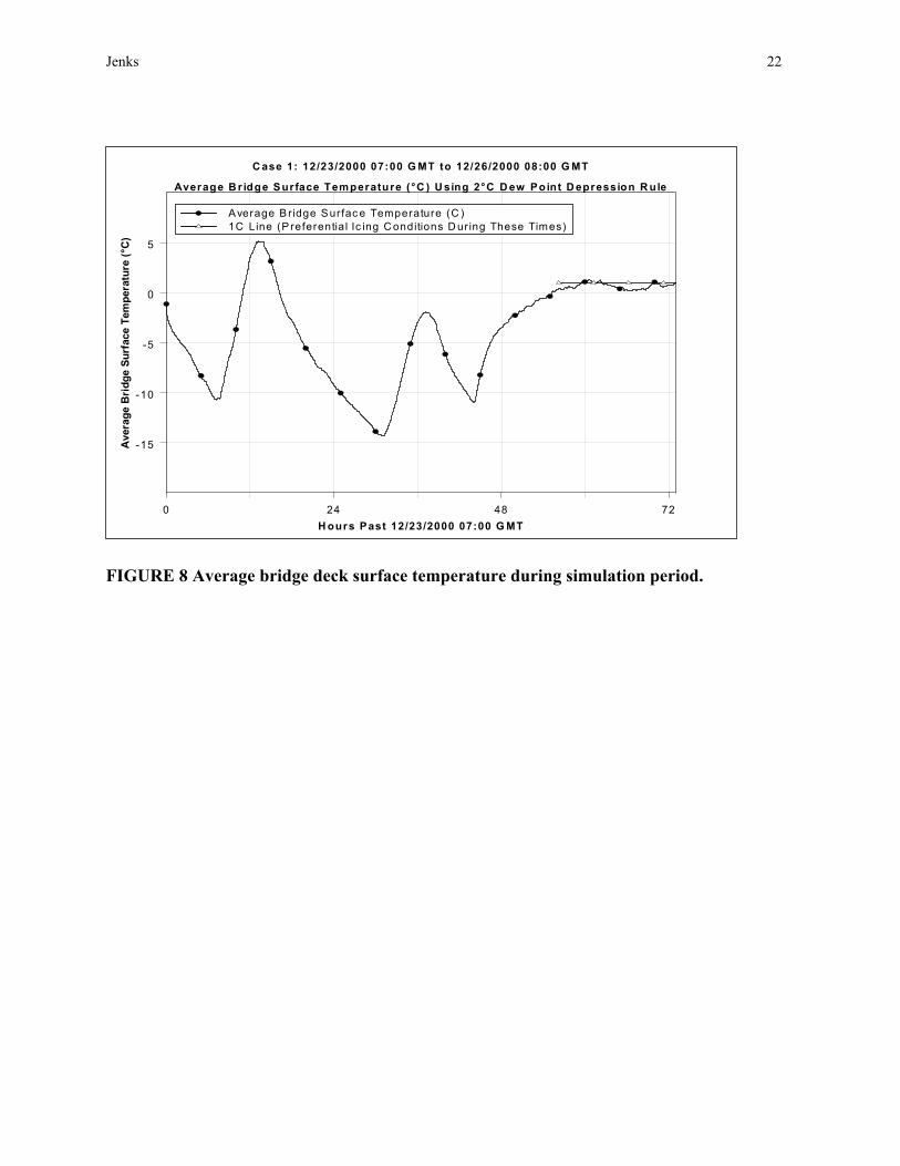
Simulation results are presented in Figure 8. A 2°C dew point depression threshold was used. The 1°C line in Fig. 8 indicates periods when the potential for preferential icing was detected. As evident in Fig. 8, the control system was able to maintain the average surface temperature within 1°C of the desired temperature.

The bridge deck heating system was not turned on until approximately 44 hours into the simulation. Approximately 12 hours were required after the heating system was first engaged to raise the average surface temperature to the desired value. Although not shown in any of the figures, the heating system was operating at maximum capacity (50°C bridge loop supply temperature) for most of the time that heating was required. Although the control performance for this case was good, from a control engineering viewpoint operating the heating system at maximum capacity for an extended time is not desirable. Had the ambient conditions been slightly more severe on December 25, the controller would not have been able to increase the bridge loop supply temperature to compensate. This is especially apparent at 67 hours past the start time when the average surface temperature was just above 0°C with the bridge loop supply temperature at the upper limit. This simulation suggests that the bridge deck heating system is slightly undersized.

CONCLUSIONS AND FUTURE WORK

Simulations indicate the control system can proactively prevent bridge deck icing. This performance is primarily the result of three key factors. First, real-time weather forecasts have been integrated into the control system, facilitating reliable predictions of future bridge deck behavior. Secondly, the MPC technique is proactive, which is especially important for controlling slow processes like a heated bridge deck. Last, a first-principles model of the bridge deck is available for use by the MPC scheme. The control scheme is generic and can be conceptually applied with any type of bridge heating technology.

Work is underway to further improve control performance. Key issues include: 1) the dew point thresholding method, 2) dealing with variation between sequential forecasts, 3) improving the robustness of the system with regard to solar radiation, and 4) addition of

Jenks 10

adaptive capability. The controller will be used to operate the heating system for the one-quarter scale test bridge on the OSU campus during the winter of 2002-03. Results will be published after the data have been collected and analyzed.

ACKNOWLEDGEMENTS

This manuscript is based on work supported by the Federal Highway Administration under Grant No. DTFH6-1-99-X-00067. Any opinions, findings, and conclusions or recommendations expressed in this publication are those of the Authors and do not necessarily reflect the view of the Federal Highway Administration.

LIST OF REFERENCES

1. Spitler, J. D. Oklahoma State University Geothermal Smart Bridge. http://www.smartbridge.okstate.edu/. Accessed July 28, 2001.

2. Minsk, L. D. Heated Bridge Technology: Report on ISTEA Sec. 6005 Program. Publication No. FHWA-RD-99-158, U.S. Department of Transportation, Federal Highway Administration, Office of Bridge Technology, 1999.

3. Jenks, S. C. A Model Predictive Control Strategy for a Bridge Deck Heated by a Geothermal Heat Pump System. M.S. Thesis. Oklahoma State University, Stillwater, OK, 2001.

4. Richalet, J. A., A. Rault, J. D. Testud, and J. Papon. Model Predictive Heuristic Control: Applications to Industrial Processes. Automatica, Vol. 14, 1978, pp. 413-428.

5. Cutler, C. R. and B. L. Ramaker. Dynamic Matrix Control - a Computer Control Algorithm. Proceedings of AIChE National Meeting. Houston, TX. 1979.

6. Qin, S. J. and T. A. Badgwell. An Overview of Industrial Model Predictive Control Technology. Proceedings of Fifth International Conference on Chemical Process Control (CPC-V). Tahoe City, California. 1997. pp. 232-256.

7. Chiasson, A. Advances in Modeling of Ground-Source Heat Pump Systems. M.S. Thesis. Oklahoma State University, Stillwater, OK, 1999.

8. Ramamoorthy, M. Applications of Hybrid Ground Source Heat Pump Systems to Buildings and Bridge Decks. M.S. Thesis. Oklahoma State University, Stillwater, OK, 2001.

9. Spitler, J. D. and M. Ramamoorthy. Bridge Deck Deicing Using Geothermal Heat Pumps. Proceedings of Heat Pumps in Cold Climates IV International Conference. Alymer, Quebec. 2000.

10. Chiasson, A. and J. D. Spitler. A Modeling Approach to Design of a Ground-Source Heat Pump Bridge Deck Heating System. Proceedings of 5th International Symposium on Snow Removal and Ice Control Technology. Raonoke, VA. 2000.

Jenks 11

11. Liu, X., S. J. Rees, and J. D. Spitler. Simulation of a Geothermal Bridge Deck Anti-Icing System and Experimental Validation. Proceedings of TRB 82nd Annual Meeting. Washington, DC. 2003.

12. Brock, F. V., K. C. Crawford, R. L. Elliott, G. W. Cuperus, S. J. Stadler, H. L. Johnson, and M. D. Eilts. The Oklahoma Mesonet, a Technical Overview. Journal of Atmospheric and Oceanic Technology, Vol. 12, No. 1, 1995, pp. 5-19.

13. Elliott, R. L., F. V. Brock, M. L. Stone, and S. L. Harp. Configuration Decisions for an Automated Weather Station Network. Applied Engineering in Agriculture, Vol. 10, No. 1, 1994, pp. 45-51.

14. Benjamin, S. G., J. M. Brown, K. J. Brundage, B. E. Schwartz, T. G. Smirnova, and T. L. Smith. RUC-2: The Rapid Update Cycle - Version 2. August 31, 1998. http://maps.fsl.noaa.gov/ruc2.tpb.html. Accessed July 28, 2001.

15. Benjamin, S. G., J. M. Brown, K. J. Brundage, D. Devenyi, G. A. Grell, D. Kim, B. E. Schwartz, T. G. Smirnova, T. L. Smith, S. S. Weygandt, and G. S. Manikin. NWS Technical Procedures Bulletin No. 490: RUC20 - the 20-km Version of the Rapid Update Cycle. May 16, 2002. http://ruc.fsl.noaa.gov/ppt_pres/RUC20-tpb.pdf. Accessed November 15, 2002.

16. Benjamin, S. G. Present and Future of the Rapid Update Cycle. February 9, 2000. http://maps.fsl.noaa.gov/CWSU/ruc_feb00_CWSU_files/v3_document.htm. Accessed July 28, 2001.

17. Marlin, T. E. Process Control: Designing Processes and Control Systems for Dynamic Performance, 2nd ed. McGraw Hill, New York, 2000.

Jenks 12

LIST OF TABLES

TABLE 1 Control System Summary for Existing Heated Bridge Decks

TABLE 2 Parameter Values and Weather Conditions Used to Generate the Dynamic Bridge Deck Model for the Simulation Results

LIST OF FIGURES

FIGURE 1 Smart Bridge heating system: A) Hydronically-heated bridge deck, B) Bridge loop circulating pump, C) Heat pump, D) Ground loop circulating pump, E) Ground loop heat exchanger, F) Controller.

FIGURE 2 MPC prediction of bridge deck temperature in the absence of any changes to bridge loop supply temperature.

FIGURE 3 Example of reference trajectory for desired bridge deck temperature.

FIGURE 4 Air and sky temperatures during simulation period.

FIGURE 5 Solar radiation during simulation period.

FIGURE 6 Precipitation rate during simulation period.

FIGURE 7 Dew Point depression during simulation period.

FIGURE 8 Average bridge deck surface temperature during simulation period.

Jenks 13

TABLE 1 Control System Summary for Existing Heated Bridge Decks

Bridge Conditions Required to Turn Heating System

ON

Conditions Required to Turn Heating System

OFF

Tenth Street Pedestrian Viaduct – Lincoln, Nebraska

Pavement T < 39°F AND

Air T < 36°F AND

Moisture on Bridge Deck

Pavement Temperature > 55°F

Silver Creek – Salem, Oregon (control rules partially

proprietary)

Air T < Specified Value AND

Moisture on Bridge Deck

Air T > 35-37°F OR

Pavement T > Specified Value

Highland Interchange – Portland, Oregon

20°F < Air T < 33°F AND

Dew Point > 0°F Unknown

Second Street Overcrossing – Hood River, Oregon

Air T < 35°F AND

Relative Humidity > 95%

30-minute minimum runtime AND

Pavement T > 36°F

U.S. 287 – Amarillo, Texas Pavement T < 35°F

AND Precipitation Forecast

Unknown

Route 60 Bridge – Amherst County, Virginia

Snow or Ice on Pavement OR

Precipitation Present AND Air T < 35°F OR

Moisture on Bridge Deck AND Pavement T < 35°F

No Moisture on Pavement for 10 minutes

OR Pavement T > 40°F

Jenks 14

TABLE 2 Parameter Values and Weather Conditions Used to Generate the Dynamic Bridge Deck Model for the Simulation Results

Bridge Deck Model Parameter Values

Pavement Length = 9.144 m Absorptivity Coefficient = 0.6

Pavement Width = 6.096 m Cp,Layer 1 = 2.2x106 J/m3 °C

Slab Orientation = 6° from North Cp, Layer 2 = 0 J/m3 °C

Pavement Thickness = 0.1524 m kPipe = 0.439 W/m °C

Pipe Spacing = 0.3048 m Wall Thickness of Pipe 1.5875x10-3 m

Pipe Diameter = 0.01905 m Fluid Type 2 = propylene glycol water solution

Pipe Depth Below Surface = 0.0889 m Weight % GS-4 = 42%

Depth to Interface 1 = 15 m Number of Flow Circuits = 10

kLayer 1 = 1.618041 W/m °C Length of Pipe Per Circuit = 19.811 m

kLayer 2 = 0 W/m °C Transient Time Step = 20 sec

Emmissivity Coefficient = 0.9 Bottom Boundary Condition 1 = convection type

Minimum Flow Condition = 0 kg/sec

Weather Inputs

Ambient Air Temperature = -13°C Solar Angle of Incidence = 0.785 radians

Relative Humidity = 18% Snowfall Rate = 6.35 mm/hr (water equiv)

Wind Speed = 0 m/s Rainfall Rate = 6.35 mm/hr (water equiv)

Wind Direction = 0° from North Sky Temperature = -36.6 °C

Solar Radiation = 0 W/m2

Jenks 15

Controller Heat Pump

A

F

E

D

C

B

FIGURE 1 Smart Bridge heating system: A) Hydronically-heated bridge deck, B) Bridge loop circulating pump, C) Heat pump, D) Ground loop circulating pump, E) Ground loop heat exchanger, F) Controller.

Jenks 16

Past Future

50

40

30

20

10

Brid

ge L

oop

Supp

lyTe

mpe

ratu

re (°

C)

Ave

rage

Brid

ge D

eck

Surf

ace

Tem

pera

ture

(°C

) 10

0

-10

Time12 Hours In Future

Assume No Future Control Action

Predicted Bridge Deck Response toForecased Weather Conditions and

No Future Control Action-20

yCV

MV

FIGURE 2 MPC Prediction of bridge deck temperature in the absence of any changes to bridge loop supply temperature.

Jenks 17

Ave

rage

Brid

ge D

eck

Surf

ace

Tem

pera

ture

(°C

)

10

0

-10

Time (hrs into future)

-20

1°C

Preferential Icing Likely During These Intervals

Slope of TemperatureRamp is User-Specified

{1-hr Safety Cushion Before FirstIndication of Preferential Icing

r

541 2 3 1096 7 8 12110

Past MeasuredValues

FIGURE 3 Example of reference trajectory for desired bridge deck temperature.

Jenks 18

0 24 48 7H ours Past 12/23/2000 07:00 G MT

2

-30

-20

-10

0

10

Tem

pera

ture

(°C

)

C ase 1: 12/23/2000 07:00 G MT to 12/26/2000 08:00 G MT

Air Temperature (°C ) and Sky Tem perature (°C )

Air Temperature (C )Sky Temperature (C )

FIGURE 4 Air and sky temperatures during simulation period.

Jenks 19

0 24 48 7H ours Past 12/12/2000 07:00 G MT

20

100

200

300

400

500

600

Sola

r R

adia

tion

(W/m

2 )

C ase 1: 12/23/2000 07:00 G MT to 12/26/2000 08:00 G MT

S olar R adiation (W /m 2)

FIGURE 5 Solar radiation during simulation period.

Jenks 20

0 24 48H ours Past 12/23/2000 07:00 G MT

720

1

2

3

4

Prec

ipita

tion

Rat

e (m

m/h

r)

C ase 1: 12/23/2000 07:00 G MT to 12/26/2000 08:00 G MT

P recip itat ion R ate (m m/hr )

FIGURE 6 Precipitation rate during simulation period.

Jenks 21

0 24 48 7

H ours P ast 12/23/2000 07:00 G MT

20

2

4

6

8

10

Dew

Poi

nt D

epre

ssio

n (°

C)

C ase 1: 12/23/2000 07:00 G MT to 12/26/2000 08:00 G MT

D ew Point D epression (°C )

FIGURE 7 Dew point depression during simulation period.

Jenks 22

0 24 48 7H ours Past 12/23/2000 07:00 G MT

2

-15

-10

-5

0

5

Ave

rage

Bri

dge

Surf

ace

Tem

pera

ture

(°C

)

C ase 1: 12/23/2000 07:00 G MT to 12/26/2000 08:00 G MT

Average B r idge S urface Temperature (°C ) U sing 2°C D ew Point D epression R ule

Average B r idge S urfac e Temperature (C )1C Line (P referentia l Ic ing C onditions D ur ing These Times)

FIGURE 8 Average bridge deck surface temperature during simulation period.