Smart Contracts and External Financing - banque-france.fr
59
"Smart" Contracts and External Financing Katrin Tinn Imperial College Business School First draft: October 2017; This draft: October 2018 Abstract Hash-linked timestamping is the key feature behind blockchain. It enhances trust as it en- ables contracting parties to have common and reliable records of transactions and of their timing. I develop a model of raising external nancing where, due to this new technology, some tradi- tional contracting frictions are not present. However, there are informational frictions whereby borrowers learn from data frequently, which a/ects their e/ort incentives. I identify conditions under which contracts benet from being "smart", i.e., self-adjusting based on timestamps. I further show that increasing the frequency of learning makes traditional assets, e.g., debt and equity, costlier and more restrictive. Keywords: blockchain, smart contracts, FinTech, contract design, Bayesian learning, prot- sharing, equity, debt, dynamic moral hazard. JEL codes: D82, D86, G23, G32, G35 I would like to thank Franklin Allen, Gilles Chemla, Lin William Cong (discussant), Alfonso Delgado De Molina Rius, Leonardo Gambacorta (discussant), Denis Gromb, Zhiguo He, Michael Huth, Andrei Kirilenko, Andreas Park, Dmitry Orlov, Chester Spatt (discussant), Peter Zimmerman (discussant), Pavel Zryumov, and the audiences at Ox- FIT 2018, European Economic Association Annual Meeting 2018, The Western Finance Association Annual Meeting 2018, FinTech, Credit and the Future of Banking Conference 2018, The First Annual Toronto FinTech Conference 2017, Warwick Congress, Bank of Estonia and Imperial College Business School for helpful comments. Contact: [email protected]; Finance Department, Imperial College Business School, Imperial College, South Kensington Campus, London SW7 2AZ, UK 1
Transcript of Smart Contracts and External Financing - banque-france.fr

"Smart" Contracts and External Financing
Katrin Tinn∗
Imperial College Business School
First draft: October 2017; This draft: October 2018
Abstract
Hash-linked timestamping is the key feature behind blockchain. It enhances trust as it en-ables contracting parties to have common and reliable records of transactions and of their timing.I develop a model of raising external financing where, due to this new technology, some tradi-tional contracting frictions are not present. However, there are informational frictions wherebyborrowers learn from data frequently, which affects their effort incentives. I identify conditionsunder which contracts benefit from being "smart", i.e., self-adjusting based on timestamps. Ifurther show that increasing the frequency of learning makes traditional assets, e.g., debt andequity, costlier and more restrictive.
Keywords: blockchain, smart contracts, FinTech, contract design, Bayesian learning, profit-sharing, equity, debt, dynamic moral hazard.
JEL codes: D82, D86, G23, G32, G35
∗I would like to thank Franklin Allen, Gilles Chemla, Lin William Cong (discussant), Alfonso Delgado De MolinaRius, Leonardo Gambacorta (discussant), Denis Gromb, Zhiguo He, Michael Huth, Andrei Kirilenko, Andreas Park,Dmitry Orlov, Chester Spatt (discussant), Peter Zimmerman (discussant), Pavel Zryumov, and the audiences at Ox-FIT 2018, European Economic Association Annual Meeting 2018, The Western Finance Association Annual Meeting2018, FinTech, Credit and the Future of Banking Conference 2018, The First Annual Toronto FinTech Conference2017, Warwick Congress, Bank of Estonia and Imperial College Business School for helpful comments.Contact: [email protected]; Finance Department, Imperial College Business School, Imperial College, SouthKensington Campus, London SW7 2AZ, UK
1

1 Introduction
An important criterion for assessing the relevance of new technologies related to Finance (some-
times called "FinTech") is whether these technologies make access to external financing easier for
firms and individuals who lack internal resources and/or who find it diffi cult to pledge future cash
flows in return for the funds needed for an investment. Blockchain is seen as one of these new
promising technologies for raising financing, as, quoting Casey and Vigna in MIT Technology Re-
view May/June 2018, blockchain "is all about creating one priceless asset: trust". "Lack of trust"
is well known in Finance and Economics to be the prime reason why external financing can only
be accessed by those with enough own assets (see e.g., Tirole 2006). It is also the main reason
why scarce and arguably expensive venture capital funding has been the best source of innovation
financing (see e.g., Lerner et. al. 2012). More fundamentally, lack of trust is at the root of the
fundamental frictions that make financial instruments necessary in the first place (see e.g., Kiyotaki
and Moore 2002).
Blockchain technology could indeed enhance trust in the context of external financing by over-
coming some traditional financing frictions that exist due to lack of cash flow pledgeability and
commitment.1 The key distinguishing feature of blockchain is hash-linked timestamping, the tech-
nical details of which are further discussed in Appendix A. In essence, blockchain is a secure
ledger/database which maintains a reliable, shareable and time-stamped record of transactions,
ownership and rights, enabling contracting parties to have a common and verifiable history of
events. Blockchain further helps contract enforcement as it can verifiably record and facilitate the
execution of actions that are predetermined by contracting agents (via a pre-agreed, recorded and
shared computer code), and it is an enabler for the development of “smart contracts”, i.e. contracts
which can automatically self-adjust and execute pre-determined actions based on incoming data.2
1Number of these benefits have also been pointed out by academics and practicioners (see e.g., Catalini and Gans2017; Yermack 2015, Harvey 2016, PwC 2016, Deloitte 2016, Dhar and Bose 2016).
2There are real world examples of this: notable examples of platforms that incorporate smart contract functionalityare Ethereum and the Hyperledger project. Ethereum is based on a permissionless and decentralized verificationmechanism in the spirit of the blockchain technology behind bitcoin. Hyperledger is an open-source Linux basedcommunity that advocates permissioned (members-only) verification mechanisms and is supported by technologyfirms such as IBM and Cisco, as well as financial services providers such as JP Morgan, SWIFT and ABN Amroamong others. While there are trade-offs in terms of costs and cryptographic security, both approaches enable similarcore benefits
2

While the broad definition of "smart contracts" includes the possibility of executing a standard
traditional financing contracts, e.g., a debt contract, automatically, it would not be a fundamentally
different contract. For this reason, I will call a contract "smart" in this paper if it relies on
timestamps and chronological order at which cash flows arrive: that is, the payoffs are different
depending on the sequence at which cash flows arrive, even if the total cash flows generated are
the same.3 One on the main goals of this paper is to identify conditions under which such "smart"
contract makes access to external financing easier.
I develop a model of raising external financing in an environment where blockchain enables the
borrower (an entrepreneur or individual) to credibly pledge the future cash-flows and to pre-commit
to any, possibly "smart" financing contract. While blockchain based financing contracts can rely
on richer state space compared to traditional contracts, which depend on cash flows generated
over a relatively longer period of time, such blockchain-based contracts would nevertheless not
be complete. This is because generating cash flows still requires human effort that is neither
contractible nor verifiable.
Furthermore, I explore the effect of more frequent learning from cash flows on optimal contracts
as well as on standard traditional assets. Indeed, there is a trend towards better data analysis
capabilities that enable firms to learn about their future prospects from incoming cash flows more
frequently. Blockchain based record keeping could enhance such frequent learning. Learning from
data in turn affects the effort incentives of entrepreneurs, and more accurate information does
not necessarily make contracting easier (see e.g., Hirshleifer 1971 in the context of insurance, and
Kaplan 2006 and Dang et. al. 2017 in the context of banking).
To be specific, I consider a setting where an entrepreneur (the borrower) can develop a project
that will enable her/him to sell new products or services (called "widgets" in this paper) to poten-
tially interested customers. The project requires a fixed investment and the borrower may need to
or prefer to use external financing to cover this cost. There is no information asymmetry between
3This timing factor differentiates blockchain records from audited accounting records, which aim to ensure that theaggregate total in- and outflows are correctly recorded over a relatively long period of time. This makes contracting onproject specific cash flows and their arrival times not feasible in traditional environments. This is further complicatedwhen firms strategically time their earnings reporting and information disclosure (see e.g., Bartov, 1993 and Healyand Palepu, 2000).
3

lenders and borrower at the time on signing the contract, but whether or not the borrower made
efforts is his private information. I also assume that raising financing is product (project) specific
rather than firm specific, i.e., the entrepreneur pledges cash flows related to developing a specific
product (e.g., as in the case of many forms of crowdfunding). This guarantees that incoming cash
flows, effectively the sales records, is something possible to record on blockchain and to contract
on.
A key feature of my model is that the borrower cannot influence the preferences of his target
consumers and takes the distribution of potential sales opportunities as given: these are determined
by the fundamental characteristics of the target market and the widget. For example, entrepreneurs,
especially start-up firms, often target a market of limited size and face uncertainty about whether
their target consumers value their product, and how easily they can find consumers who value their
product. When the prime source of uncertainty is about the firm not knowing the preferences of
target consumers likely to have similar taste, then successful past sales tend to raise the borrower’s
expectations about future sales prospects. If instead the prime source of uncertainty is about how
quickly the firm will find its target in a limited market, then successful past sales tend to lower
the borrower’s expectations about future sales prospects. In my main setting I do not impose the
most usual restrictions on the joint distribution of potential sales opportunities, and I explore how
the core properties of potential sales distribution determine the desirable financing contracts in the
described environment. These features also distinguish my model from other contracting papers
with dynamic moral hazard. I also allow effort cost to follow any dynamics.
I show that it is crucial to distinguish an environment where potential sales are stochastically
affi liated (log-supermodular)4 from an environment where they are not. As stochastic affi liation
implies that successful past sales lead the entrepreneur to Bayesian update his beliefs about future
sales upward, I call such environment a "success raises prospects" (SRP) environment. In contrast,
a "success lowers prospects" (SLP) environment is one where sales are log-submodular, and past
sales success leads the entrepreneur to Bayesian update his beliefs about future sales downward.
4Stochastic affi liation implies monotone likelihood ratio property (see e.g., Milgrom, 1981 and Milgrom and Weber,1982), which in turn often plays a central role in principal agent models.
4

As discussed above, one determinant of whether the firm operated in SRP or SLP environment is a
type of uncertainty it faces. Furthermore, firms that produce products that have positive network
effects (e.g., a platform business) are more likely to operate in a SRP market, while those producing
items that their target consumers value because of their rarity and uniqueness (e.g., design items)
are more likely to operate in a SLP environment. While the economics and finance literature most
often focuses on environments with independent cash flow processes, and somewhat less frequently
on affi liated ones, an environment where selling can become more diffi cult after early success is
equally plausible.
I find that in all these environments the optimal contract can be represented in a relatively
simple form where each successful sale is split between the lender and the borrower according
to a dynamically adjusting splitting rule on incoming cash flows/sales revenues that depend on
the history sales up to that point. In fact, the splitting rule is determined by variables that are
predictable and can be easily and dynamically calculated by an econometric algorithm embedded in
the code that implements a "smart contract": such as the expected value of next sales conditional on
the history of past sales up to that point, and such as the expected value of sales at some point in the
future if no successful sale happens in between (i.e., a "worst case scenario analysis"). Furthermore,
the optimal contract typically benefits from being "smart" unless the following restrictive conditions
hold: effort cost is constant, potential sales are stochastically affi liated and exchangeable random
variables.5 Even when these conditions hold, the optimal contract is not-standard as the borrowers
payoff is concave in total sales. This is opposite to debt contracts or convertible notes where the
borrower’s payoff is convex in total sales. In a very special case where effort cost is constant,
and potential sales are independently and identically distributed over time, the optimal contract is
simple equity. In such case there is no learning from past sales.
I further show that there are a number of important asymmetries between SRP and SLP envi-
ronments. In SRP environment the optimal contract resembles progressive taxation whereby higher
past sales lead the borrower to have a lower claim on future profits. In order to undertake a break-
5Exchangeability requires that the joint distribution of potential sales is unaffected by reordering the realizations.It would be violated if the chances of meeting interested and uninterested consumers is not random, and if there issome cyclicality is sales prospects, for example.
5
even investment project, the borrower would need to invest some own funds. The optimal contract
needs to maintain effort incentives in states where the borrower is relatively pessimistic about his
future prospects. This creates a manipulation possibility whereby the borrowed strategically with-
olds the effort anticipating better contractual terms, similar to what is called "information rents" in
some contract theory papers discussed below. Own investment is essentially needed to offset these
information rents. In contracts, all positive NPV projects can be financed without the need for the
entrepreneur’s own funds in a SLP environment. This is because a contract based on timestamped
records can perfectly offset any distortions due to learning. The optimal contract in a SLP environ-
ment resembles a merit based scheme whereby past success should give the entrepreneur a right to
a higher share of the next sale, and vice versa, to offset the fact that past success indicates greater
diffi culties to achieve further success.
This paper shows that under blockchain technology, the economic outcomes are closer to those
in the frictionless market of Modigliani and Miller (1958, 1963) in the sense that the expected profit
of a borrower who obtains external financing is as high as it would be in a frictionless market, and
using own funds is not cheaper than external financing for most borrowers. Furthermore, borrowers
can finance all profitable investment projects with minimal own funds, and even zero own funds
in some informational environments. However, in contrast to Modigliani and Miller (1958, 1963)
all financing contracts are not equivalent. I show that the reason why debt is suboptimal in
this environment is that debt gives poor incentives to continue making efforts following unlucky
outcomes (similar to debt overhang). Anticipating no effort in some states will make the investors
more reluctant to lend. I also show that equity is suboptimal whenever learning from past sales
reveals information about future sales prospects. With simple equity, the borrower would need to
have high enough own share of revenues to maintain effort incentives in the "worst case scenario",
while he would prefer to accept a contract that gives him a lower share in the "best case scenario"
in return for the benefit of accessing external financing more easily ex-ante. Furthermore, I show
that both debt and equity become increasingly expensive when the borrower learn and adjusts his
effort more frequently. For this reason I argue that the "smart contracts" facilitated by blockchain
technology should not just be seen as a way to make the execution of financing contracts cheaper,
6

but could be seen as a counter force to mitigate the negative forces generated by more frequent
learning.
The early literature on credit rationing and financial contracting (see e.g., Tirole, 2016 and Allen
and Winton, 1995, for reviews) has often found debt or debt-like contracts to be the "second best"
optimal contracts in settings with realistic contracting frictions in traditional environments. This
reinforces the idea that the new technologies considered in this paper have the potential to funda-
mentally change the dominant financing frictions and consequently lead to different ways to raise
external funds. One of the prominent theoretical arguments for the optimality of debt stems from
the costly state verification literature (see e.g., Townsend, 1979, Diamond, 1984, Gale and Hellwig,
1985, Mookherjee and Png, 1989.), which highlights that debt contracts enable effi cient monitoring
and minimize verification costs. As argued above, the key promise of blockchain technology is to
eliminate (or greatly reduce) these costs by guaranteeing easily verifiable and commonly shared
records of transactions. Debt also features as optimal in static models of moral hazard where the
aggregate cash flows are assumed to be verifiable, such as in Innes (1990), and in settings building
on this. The crucial difference with my paper is that Innes (1990) does not consider the effect of
frequent learning and effort decisions and assumes that the borrower makes his effort choice once
and for all, just after signing the contract. As argued above, entrepreneurs are likely to learn from
incoming data and can adjust their effort frequently after signing the contracts, which is the prime
reason that makes debt contracts increasingly costly in my setting. Indeed, Chiesa (1992) extends
Innes’s setting to allows the borrower to observe information before making an one-off effort de-
cision and shows that debt combined with warrants does better than simple debt for a similar
reason as in my paper: debt contracts give bad incentives to make an effort after bad news. Other
important arguments for debt emphasize the robustness of these contracts to renegotiations (see
e.g., Hermalin and Katz, 1991, and Dewatripont et. al., 2003) and enforcement (see e.g., Hart and
Moore, 1998) - both of these frictions could arguably be eliminated by smart contracts, or at least
be of second order importance for an individual small borrower that uses blockchain-based smart
contracts.
This paper further relates to the literature on dynamic moral hazard, and the associated lit-
7

erature on principal-agent problems. My paper emphasizes that to fully benefit from blockchain
technology, the borrowers and lenders would need to write contracts that depend not just on sales
that happened, but also on when they happened. In this context it is important to clarify the con-
nection of my paper with Holmström and Milgrom (1987), often cited for justifying the optimality
of linear contracts. However, the more general insight in their paper is that in many principal agent
settings, the optimal dynamic scheme should only depend on the number of times a particular out-
come occurs, and not on the order in which these outcomes occur, i.e., a sales history {0, 1, 1}
should give the same payoff as a sales history {1, 1, 0}. If that would be the case in my setting,
time-stamping would not matter. The crucial difference is that the potential sales distribution is
realistically not under the full control of the entrepreneur: she/he cannot dictate the preferences of
her/his target consumers regardless of her/his effort, and can only decide whether to explore the
opportunity or not. This is the main reason why distributional properties of sales process matter.
Furthermore, the results of Holmström and Milgrom (1987) are derived in a setting where incentive
compatibility constraints bind. When "success lowers prospects", I show that the borrower’s effort
is easy to incentivise, because incentive compatibility constraints do not bind, and the binding
constraint is the participation constraint.
In my model the possibility to commit a flexible repayment schedule enables the borrower to
optimally manage the risks associated with learning by enabling him to trade off a lower share
of profits in states he is more optimistic about the future prospects with a higher share of profits
in the states that he is more pessimistic about future prospects. This finding relates to Palfey
and Spatt (1985) who highlights the risk-sharing benefits of long-term contracting compared to a
sequence of short-term contracts in an insurance market where contracting parties can learn about
underlying risks. Dunn and Spatt (1988) further the prevalence of long-term contracting in the
context of mortage contracts. While mortgage and other loan contracts contracts sometimes allow
some flexibility such as the possibility of early prepayment and adjustible rates, these contracts are
typically not fully contingent on borrower income or cash flows. While the contracts in my setting
are contingent on realized cash flows, the contracts are not complete as verifying and contracting
on effort is not possible.
8
More recent advances in dynamic moral hazard and financing contracts also highlight the ben-
efits of more nuanced and history dependent financing contracts, but tend to also assume greater
control of agents over the cash flow process compared to the setting considered in this paper and
more restrictive cash flow processes conditional on the agent’s actions. For example, DeMarzo and
Fishman (2007) and Biais et. al. (2007, 2011) find that financing contracts that combine equity,
debt, and credit line or well managed cash reserves are optimal in a dynamic setting where cash flow
process conditional on effort is i.i.d. across time. DeMarzo and Sannikov (2016) consider a setting
where cash flow process is governed by a Brownian motion, which is a parametric example of a SRP
environment. In their paper, as in my paper, there are "information rents" and equity contract is
optimal under some very specific circumstances. Similar information rents also feature in He et.
al (2010) and Prat and Jovanovic (2014) that also use Brownian motion. These settings generally
do not explore the SLP environment and the role of frequency of learning. It seems plausible that
the combination of standard assets that constitutes the optimal contract in these papers could be
also expressed as a dynamically adjusting profit sharing contract. At the same time traditional
assets, that do not adjust based on each cash flow, cannot replicate the self-adjusting profit sharing
contracts in all the informational environments considered in this paper. The latter is because
statistical dependencies between the firm’s target market and target consumer preferences can be
too complex to maintain effort incentive under a limited set of assets, while the effect of learning
on incentives is nevertheless predictable.
Interestingly, the finding that the optimal contract could take the form of a time-varying share
contract features in Bergemann and Hege (1998). Their paper considers dynamic moral hazard in
a different context, where moral hazard is not associated with an effort to generate sales, but with
the possibility to divert investor’s funds instead of investing these in the project development before
the known sales outcome is generated. These result are complementary to those in my paper. An
important difference is that despite the fact that a product development process resembles a "success
raises prospects" environment, a pre-sales product development requires continued investments
which make the optimal contract in their paper to be more similar to the one applicable to "success
lowers prospects" environment.
9

There is also an emerging literature on blockchain in economics and finance, which focuses on
different aspects of blockchain. Kroll et. al (2013), Biais et. al. (2018), Cong et. al. (2018), Easley
et. al (2018) and Saleh (2008) focus on the viability of decentralized verification mechanisms.
Malinova and Park (2017) explore different market designs of blockchain in the context of asset
trading. Yermack (2017) and Catalini and Gans (2017) discuss possible applications of blockchain
technology more generally. Cong and He (2018) focus on the role of smart contracts in the context
of tacit collusion and industrial organization, rather than a financial contracting perspective. In
particular, they highlight the consideration that blockchain records could reveal information to
competitors. This problem would be avoided in a permissioned verification system which does not
need sensitive details of the contract publicly available (see further on different types of blockchains
in Appendix A).
The mechanisms developed in this paper have practical relevance in the context of recently
emerged forms of fund-raising that either rely on blockchain technology directly or use platforms
that incorporate blockchain technology to facilitate contracting and borrower-lender interactions.
A noticeable example is a subset of initial coin offerings (ICOs) which involve issuing tokens that
give the participants rights on the firm’s revenues, profits or shares.6 Another example is a set of
emerging FinTech platforms that act as a new type of intermediaries that facilitate specific financing
contracts, and typically use blockchain technology as part of their business model.7 These new
forms of fund-raising are growing fast and are often based on equity or profit sharing contracts.
While a full implementation of blockchain based financing contracts may require wider adoption of
this technology, hybrid models that benefit from some aspects of this technology, while relying on
6According to www.icodata.io, the overall funds raised via ICOs stood at $6 billion in 2017 (in comparison to $90million in 2016), exceeding the early stage venture capital investment volume (see e.g., See Oscar Williams-Grut atBusiness Insider, January 31, 2018), and is already around $3.9 billion in January-April 2018. According to a recentpaper by Adhami, Giudici and Martinazzi (forthcoming) tokens offering profit rights are already quite common andconstitute 26.1% of ICOs surveyed, and they find that offering profit (or service) tokens, increases the probabilityof the success of fund-raising via an ICO. Other common types of tokens include governance rights or the right toaccess the platform service, latter of which resembles reward-based crowdfunding (see e.g., Li and Mann (2018)).
7To name a few that have attracted attention: Funderbeam (https://www.funderbeam.com) enables equity in-vestments in the spirit of venture capital investments combined with blockchain-based secondary market trading,Corl (https://corl.io) proposes revenue sharing contracts where some of the contractual terms, such as the term,adjust depending on realized revenues. There are also platforms that facilitate debt contracts, such as SALT(https://www.saltlending.com), which facilitates blockchain based lending and enables the use of crypto-currenciesand -tokens as collateral.
10

centralized parties for up-to-date data, or contract enforcement in other aspects, can also deliver
at least some of the benefits my model highlights.
2 The model of external financing with frequently observed cashflows
This section sets up and finds the optimal contract in a frequent learning environment where
after signing the contract the borrower (an entrepreneur or an individual) observes each widget
sale, regularly updates his beliefs about its target market, and decides whether to make efforts to
generate further sales. I assume that there is a blockchain-based ledger8, which guarantees that
there is a reliable, verifiable and timestamped record of each widget sale. The optimal contract
can therefore be any, possibly "complex", function of each realized widget sale and on when these
sales happened. Solving this contracting problem answers whether and when "smart" contracts
that benefit from timestamps enable better access to financing compared to contracts that rely on
the total cash flows generated by the project only.
Solving this problem is also a necessary step for understanding the role of more frequent learning
and decision making on accessibility to external financing under different contracts. In Section 3, I
will consider a comparable setting where the borrower observes sales and makes effort decisions less
frequently. I will then contrast the impact of more frequent learning under the optimal contract
with those that emerge if the borrower was limited to rely on raising funds using traditional assets,
such as debt and equity. I will also highlight the role of prior uncertainty in driving the differences
between "smart" contracts and traditional assets.
I will assume throughout the analysis that contracting parties pre-commit to pre-agreed con-
tractual terms. This is facilitated by blockchain (and timestamped records in particular), as the
code implementing the terms of financing contracts can be verifiably recorded as well, and it can
be made suffi ciently costly and diffi cult to change the contractual terms ex-post.
8The immediate applications involve products that need to be, or benefit from being recorded on blockchain, suchas goods sold for crypto-currencies, or benefit from being recorded on blockchain due to certification. It has beenfurther imagined that blockchain could allow the creation of a World Wide Ledger that would record all transactionsand ownership data (see e.g., Harvey 2016, Shackelford and Myers 2017, Swan 2015 and Tapscott and Tapscott 2016).
11

2.1 The setting
A would-be borrower (an entrepreneur or an individual) has a project idea that requires fixed
investment I at date 0. The borrower is risk-neutral and has own funds A, which he may choose
to invest in the project or not. Assume that lenders operate in a competitive market and there is
a representative risk-neutral lender.
If the project is pursued, the borrower can at each date t = 1, ..., T , make a potential sale
st = {0, 1}.9 The joint distribution of potential sales, p (s1, ..., sT ) , is known at date 0 to both
parties, and the only restriction on this joint distribution imposed throughout the analysis is that
all possible sequences of potential sales occur with strictly positive probability, i.e., p (s1, ..., sT ) > 0
for any sequence s1, ..., sT . While the distribution of the potential sales is determined by the nature
of the borrower’s project and the environment in which he operates, the borrower needs to make
efforts. The effort decision at t = 0, ..., T − 1 is denoted with an indicator function 1t = {1, 0},
where 1t = 1 if the borrower makes an effort, 1t = 0 otherwise, and the effort cost is et ≥ 0 in
monetary equivalent units. If the borrower chooses 1t = 0, then the sales at t + 1 are zero with
probability 1. The realized sales are denoted with st = 1t−1st.
Because the effort is neither observable nor contractible, the contract between the borrower and
the lender is a function of realized sales, st, rather than the potential sales, st. The discount rate is
normalized to 1, and I assume that et is small enough to guarantee that making an effort is always
optimal, i.e., it holds that et ≤ E [st+1|10s1, ...,1t−1st,10, ...,1t−1] for any t.
The financing contract is signed at date 0, and I assume that it is the borrower who proposes
the contract to the lenders. The contract specifies the borrower’s reward, a function w (s1, .., sT )
which depends on realized sales st for t = 1, ..., T , and the lender’s reward which is the difference
between total sales and the borrower’s reward. The borrower’s preferences depend on his expected
returns and his own investment in the project. I assume lexicographic preferences, such that
w (s1, .., sT ) % (�)w (s′1, .., s′T ) if either "E [π] > E [π′]" or "E [π] = E [π′] and A0 ≤ (<)A′0",
where E [π] is the expected net present value of the project (inclding the monetary cost of effort),
9Discrete time captures the discrete nature of blockchain records. It also takes time to confirm a transaction (thenumber of transactions confirmed per second peaks at 7 in Bitcoin network, 15 in Ethereum and 3500 in HyperledgerFabric).
12

A0 = [0, A] is the borrower’s own investment in the project under the contract w (s1, .., sT ), and
E [π′] and A′0 are the same variables under an alternative contract w (s′1, .., s′T ). The date T value
of the project for the borrower is
π = w (s1, .., sT )−A0 −T−1∑t=0
1tet. (1)
A feasible contract must satisfy the lender’s break even constraint
I −A0 = E[T∑t=1
st − w (s1, .., sT )
](2)
and the borrower makes optimal effort decisions at each date, i.e., for every t = 0, ..., T −1, it holds
that 1t = 1 if, and only if
E [π| s1, ..., st,10, ...,1t−1,1t = 1] ≥ E [π| s1, ..., st,10, ...,1t−1,1t = 0] . (3)
I also assume that there is limited liability, i.e., w (s1, .., sT ) ≥ 0.
It is worthwhile to discuss some of the features of this setting. Lexicographic preferences
cover the standard case where the borrower just maximizes his expected returns from his project.
However, as the blockchain is assumed to eliminate a number of financing frictions, we may need
more structure to compare contracts that give the same expected profit. It is then natural to
consider that the borrower would prefer to risk losing as little of his own funds as possible, while
still trying out his project idea. An additional advantage is that the optimal contract derived under
lexicographic preferences is one that maximizes the availability of outside financing to borrowers
with little own assets, and thus minimizes credit rationing (see further in Section 2.2).
The incentive compatibility constraint (3) highlights that when making an effort decision at
date t, the borrower has additional information compared to date 0 - he knows whether he made
an effort in past, and what the sales were at dates when he tried to actively sell. Because the effort
is not verifiable, the contract cannot distinguish between zero sales due to bad luck or due to lack
of effort, and the borrower has superior information when making his optimal effort decisions. As
π in (1) depends on all efforts between date 0 and T , it is also possible that when making the the
effort decision at t, the borrower expects this decision to affects his future effort decisions.
13

2.1.1 Key distributional properties and related examples of target markets
While the main setting imposes minimal restrictions on the joint distribution of potential sales,
p (s1, ..., sT ), it is useful to recall the definitions of some useful properties of random variables to
structure the analysis, and to consider some examples that highlight economic forces that generate
these distributional properties.
Definition 1 Given n random variables jointly distributed in Rn according to distribution func-
tion f , let x = (x1, ..., xn) and y = (y1, ..., yn) be two points in Rn. The random variables are
stochastically affi liated if, and only if for every x and y
f (x ∧ y) f (x ∨ y) ≥ f (x) f (y) , where (4)
x ∧ y = (min (x1, y1) , ...,min (xn, yn))
x ∨ y = (max (x1, y1) , ...,max (xn, yn)) ,
i.e., the joint distribution is log-supermodular. If random variables have this property I will refer
to the environment as a "success raises prospects (SRP)" environment. If the inequality in
(4) is reversed, then the joint distribution is log-submodular and I will refer to the environment as
a "success lowers prospects (SLP)" environment.
Stochastic affi liation is a strong form of positive correlation (which implies the monotone like-
lihood ratio property). It can be called a "success raises prospects (SRP)" environment, because
a successful sale at date t makes the borrower to revise upwards his beliefs about the probability
of making successful sales in the subsequent periods. In the opposite case of stochastic affi liation,
the log-submodular potential sales process captures a market where early sales success indicates
a greater diffi culty to find future sales opportunities and can therefore be called a "success lowers
prospects (SLP)" environment.
Start-up projects often involve a new niche product that targets a market with a finite size,
and there is likely to be some uncertainty regarding target consumer preferences as well as how
easy it is to find potentially interested consumers. As an example of a framework that incorporates
14

both features, consider that after investing the entrepreneur will aim to sell his widget in a market
with N consumers, whose type and preferences are not perfectly known to the entrepreneur (and
the lenders). Suppose that consumers in this market arrive in a random sequence and that the
consumer who arrives at date t is of type τ t = {NI, PI}, where the type τ t = NI consumer is not
interested in the widget with probability one, and the type τ t = PI consumer is interested in buying
the widget with some unknown probability θ ∈ (0, 1]. There are K ≤ N type "PI" consumers
in this market and the preferences of type "PI" consumers are drawn from a beta distribution
θ ∼ Be (λθ0, λ (1− θ0)),10 where θ0 = E [θ] is the mean and the parameter λ measures the degree of
uncertainty regarding the unobservable preference parameter θ (lower λ meaning higher uncertainty
about θ as V ar [θ] = θ0(1−θ0)1+λ ). Preferences of type "PI" consumers are conditionally independent
and Pr (st = 1|θ, τ t = PI) = θ.
In the described environment sales are statistically dependent and a successful early sale can
both raise or lower future prospects. Which effect dominates, depends on the core parameters,
K,N, θ0 and λ, which are determined by the characteristics of the target market, and which
can be assessed based on market analysis. Appendix B.1 provides further intuition regarding these
parameters by fully characterizing the statistical dependancies between the first two potential sales.
It shows that a firm is more likely to operate in a SRP environment when its total market is large
(high N), when the firm meets potentially interested (type "PI") consumers frequently (high K/N),
when it is uncertain about type "PI" consumers preferences (low λ), and when it has low prior
expectations about their interest (low θ0). A SLP environment is more likely when the firms faces a
limited target (low N) with potentially very interested consumers (high θ0 and λ) who are diffi cult
to find (low K/N). Start-up developing innovative consumer products may be operating in either
type of environment. The key difference is whether the prime source of uncertainty has to do with
not knowing whether the firm’s potential consumers with correlated preferences value the product
(SRP), or how diffi cult it is for the firm to find all its potential consumers (SLP). For example,
when there are three consumers (N = 3), out of which two may be interested (K = 2) and each
10Beta distribution captures a wide set of prior beliefs: be it uniform Be (1, 1), hump-shaped, U-shaped, and right-or left-skewed.
15

potentially interested consumer is interested with 50% probability (θ0 = E [θ] = 0.5), then there is
a cut-off value λ = 2 such that λ < 2 implies a SRP environment and λ > 2 a SLP environment.11
If the firm sells one widget at date 1, it must have met a type "PI" consumer. On one hand this
sale lowers future prospects because the probability of meeting a type "NI" consumer next is now
higher. On the other hand this sale increases future prospects, as the consumer’s decision to buy is
a positive signal about the other "PI" consumer’s interest to buy the product as well. The second
effect is stronger when there is greater prior uncertainty about type "PI" consumer preferences
(lower λ).
Some examples used later on benefit from the two limit cases that have a convenient parametric
represtantation. One case limit case is where the firm has perfectly identified the set of potentially
interested consumers (type "PI"), i.e., K = N , but is unsure about the preferences of these con-
sumers, i.e., θ0 ∈ [0, 1] and λ is finite. This environment is always SRP. Another limit case where
there is uncertainty about when the firm will find its potentially interested consumers, i.e., K < N ,
while the preferences of potentially interested consumers are not correlated, i.e., λ → ∞.12 This
environment is always SLP.
There are other target market specific characteristics that push towards either SRP or SLP
enviroments. For example, SRP is more likely when the firm’s product exhibits positive network
effects (e.g., it has a platform business), and SLP is more likely when there are negative externalities
(e.g., the firm produces design items that consumers value as rare or limited edition products).
A further factor that can push towards SLP is possible retaliation (e.g., an advertising war) by
dominant other firms producing imperfect subsitutes to the firm’s product if the firm’s product
proves successful.
Another useful property of random variables is exchangeability:
Definition 2 Random variables X1,..., Xn are exchangeable if a sequence (X1, ..., Xn) is equal in
distribution to (Xi1 , ..., Xin) for any n! permutation i1,...,in of integers 1, .., n.
11Note that when θ0 = 0.5 the prior distribution is symmetric, and λ < 2 corresponds to U-shaped prior, λ = 2corresponds to uniform prior; λ > 2 corresponds to humpshaped prior.12 If additionally θ = θ0 = 1, then the sales process is random sampling without replacement.
16

Exchangeability in this setting means that the order at which potential sales arrive does not
affect the joint probability. For example, with three potential sales opportunities it must be the
case that joint probability p (0, 1, 1) = p (1, 1, 0) = p (1, 0, 1), etc. Intuitively, exchangeability means
that from an ex-ante perspective, potential sales opportunities are equally likely to arrive at any
t. Considering the above examples, exchangeability would be violated if the firm did not meet is
potential consumers randombly, e.g., it could face a predictably higher probability of meeting a
type τ t = PI after a launch event that involved an advertising campaign. Exchangeability would
also be violated if there was some cyclicality in sales prospects.
2.2 First best and outside financing capacity
For the first best benchmark, consider the social planner who lends the borrower I and who chooses
the borrower’s optimal effort. It turns out that any optimal contract must focus on the borrower’s
secondary motive.
Lemma 3 1) Under the first best, the borrower sets 1t = 1 for every t, and the project is undertaken
as long as I ≤ IFB = πFB, where
πFB ≡T−1∑t=0
E [st]−T−1∑t=0
et. (5)
2) Any optimal financing contract must also set 1t = 1 for every t. As the borrower’s expected
profit under the optimal contract is the same as under the first best, the optimal contract is the one
that minimizes A0.
Proof. See Appendix B.2.
The first part of Lemma 3 is intuitive as we assumed that the effort cost is small enough
that effort is always worth undertaking. The second part of Lemma 3 highlights that any optimal
contract in this setting must also guarantee the first best effort, as doing so maximizes the borrower’s
expected profit, which is his primary objective. Furthermore, lowering effort cannot lead to smaller
own investment by the borrower. Hence, under any optimal contract all borrowers with A ≥ A0
can raise financing to cover any I ≤ IFB and have as high expected profit as under the first best
(πFB). If A0 > 0, then firms with A < A0, are cannot pursue their project. Inducing first best
17

effort is achievable in this setting because cash flows are pledgeable.13 At the same time inducing
the first best effort is not trivial, as the optimal contract must satisfy the 2T − 1 dynamic incentive
compatibility constraints given by (3).
Lemma 3 further enables to simplify the contracting problem, as we can restate the problem as
one that minimizes A0, such that (3) are satisfied for 1t = 1 for every t. It is first useful to define
w (s1, .., sT ) as a contract offered by a break-even borrower with I = IFB.
Minimizing the break even investor’s own investment A0 while keeping π = πFB fixed is equiv-
alent to minimizing the break-even borrower’s reward
min{w(s1,..,sT )≥0}
E [w (s1, .., sT )] , (6)
such that the break-even borrower is willing to pursue the project
E [w (s1, .., sT )]−T−1∑t=0
et ≥ 0 (7)
and to choose first-best effort at each date t = 0, .., T − 1
E [w (s1, .., st, st+1, st+2,..., sT )− w (s1, .., st, 0, st+2,..., sT ) |s1, .., st] ≥ et. (8)
The solution of this problem will give the contract and the minimum downpayment necessary
to cover the break-even investment cost IFB, which is given by A0 = E [w (s1, .., sT )]−T−1∑t=0
et. The
difference E [w (s1, .., sT )] −T−1∑t=0
et can be interpreted as the information rent the borrower needs
to obtain to satisfy the incentive compatibility constraints given by (8) at each date t and for
any sales history up to t. The distribution of potential sales revenues determines whether positive
information rents are needed or not.
Naturally, any borrower who has fixed investment cost I < IFB is easier to incentivise. From
(2) and (5) we can find that such a borrower maximizes his preferences by choosing
A0 = max
[0,E [w (s1, .., sT )]−
T−1∑t=0
et −(IFB − I
)]. (9)
When E [w (s1, .., sT )]−T−1∑t=0
et−(IFB − I
)≥ 0, then w (s1, .., sT ) and A0 = E [w (s1, .., sT )]−
T−1∑t=0
et−(IFB − I
)consititutes the optimal contract for a borrower with I < IFB. If E [w (s1, .., sT )] −
13 Indeed, the typical reason why borrowers benefit and prefer to invest all their own funds in the project in costlystate verification literature is that cash flows are not pledgeable and the optimal contract needs to induce truthtelling.
18

T−1∑t=0
et −(IFB − I
)< 0, then the borrower obtains an additional surplus. Any contract to capture
this surplus that does not violate (3) is optimal.
2.3 Main results
2.3.1 Two date example
To develop the intuition behind the main results it is useful to first consider the case where T = 2.
There are four possible sales outcomes (s1, s2) ∈ {(0, 0) , (0, 1) , (1, 0) , (1, 1)}; the corresponding
probabilities and borrower’s rewards are p (s1, s2) and w (s1, s2) respectively. Define the marginal
probabilities as pt (1) ≡ Pr (st = 1) and pt (0) ≡ Pr (st = 0) for t = 1, 2. Note that p1 (1) = p2 (1)
if potential sales are exchangeable random variables; these probabilities may differ otherwise. We
can further expand the constraint on effort costs14
e0 ≤ E [s1] = p1 (1) ; e1 ≤ min [E [s2|s1 = 1] ,E [s2|s1 = 0]] = min[p(1,1)p1(1) ,
p(0,1)p1(0)
]. (10)
We can restate the problem (6)-(8) as
minE [w (s1, s2)] (11)
subject to the participation constraint
E [w (s1, s2)] ≥ e0 + e1 (12)
and to the three incentive compatibility constraints
E [w (s1, s2)− w (0, s2)] ≥ e0 (13)
E [w (0, s2)− w (0, 0) |s1 = 0] ≥ e1
E [w (1, s2)− w (1, 0) |s1 = 1] ≥ e1
and the non-negativity constraint w (s1, s2) ≥ 0.
The incentive compatibility constraints highlight that the borrower must always get a positive
payoff from generating the next sale. It is immediate that a contract that keeps the borrower’s
14Note that the condition e1 ≤ E [s2|11s1] requires that e1 ≤ E [s2|s1 = 0], e1 ≤ E [s2|s1 = 1] and e1 ≤ E [s2].However, the last constraint is redundant because the law of iterated expectations implies that E [s2] = p1 (1)E [s2|1]+p1 (0)E [s2|0].
19

payoff constant in some states (e.g., debt contract) cannot guarantee effort in all states and be
optimal.
The last two incentive compatibility constraints also highlight the role of learning, as these can
be written as w (s1, 1) − w (s1, 0) ≥ e1Pr(s2=1|s1) , where Pr (s2 = 1|s1) generally changes depending
on the realizations of s1, which in turn are determined by whether the borrower operates in a SRP
or SLP environment.
Proposition 4 The optimal contract of a break-even borrower depends on the joint distribution as
follows
1) In a "success raises prospects" (SRP) environment, i.e., p (1, 1) p (0, 0) ≥ p (1, 0) p (0, 1), the
borrower’s reward is
w (0, 0) = 0 (14)
w (0, 1) = e1p1 (0)
p (0, 1)
w (1, 0) =e0 − e1
p1 (1)+ w (0, 1)
p2 (1)
p1 (1)
w (1, 1) = w (1, 0) + e1p1 (1)
p (1, 1),
and he invests
A0 = e1p (1, 1) p (0, 0)− p (1, 0) p (0, 1)
p (0, 1). (15)
The project is undertaken if A ≥ A0.
2) In a "success lowers prospects" (SLP) environment, i.e., p (1, 1) p (0, 0) ≤ p (1, 0) p (0, 1), the
borrower’s reward is
w (0, 0) = 0 (16)
w (0, 1) = e1p1 (0)
p (0, 1)
w (1, 0) =e0
p1 (1)
w (1, 1) = w (1, 0) + e1p1 (1)
p (1, 1),
and he invests
A0 = 0.
20

The project is always undertaken and is fully externally financed.
Proof. See Appendix B.3.
The proof of this proposition uses the Duality and Complementary Slackness Theorems: given
the primal minimization problem above, there is a dual maximization problem. The Duality Theo-
rem implies that if both problems are feasible, both have a solution and the minimized (maximized)
value of the primal (dual) is the same. The main insights are that in a SRP environment all the in-
centive compatibility constraints (13) must be binding and the participation constraint (12) can be
slack, while in a SLP environment the participation constraint (12) must be binding and incentive
compatibility constraints can be slack (13).
Corollary 5 The optimal contract can be expressed as
w (s1, s2) = α1s1 + α2 (s1) s2,
where
α2 (s1) =e1
E [s2|s1](17)
and
α1 =
{e0−e1E[s1] + E[s2]
E[s1]α2 (0) in SRP environmente0E[s1] in SLP environment
(18)
Proof. Straightforward from (14) and (16) given Bayes’ rule and the definition of conditional
expectations.
Corollary 5 shows how the optimal contract can be expressed as a self-adjusting profit sharing
rule, where the borrower receives the share α1 and α2 (s1) of each date 1 and 2 sales, respectively,
and the lender receives the remainder 1− α1 and 1− α2 (s1).15 It is a "smart" contract as long as
α2 (0) 6= α2 (1).
Whether or not such a smart contract brings added value compared to contracting on aggregate
cash flows, boils down to assessing whether w (0, 1) = w (1, 0) is consistent with the optimal con-
tract. In a SRP environment, we can see from (14) that w (0, 1) = w (1, 0) generally requires both:15We can see that if the cost of effort is constant, i.e., e0 = e1 = e, and sales are are exchangeable random variables,
then the borrower and lender can immediately split the revenue from each sale, as α1, α2 (s1) ≤ 1, (see (10)). Moregenerally, the contract can always take advantage of an escrow account if α1 > 1 and temporarily withold some fundsuntil the date 2 outcome is realized as well.
21

sales revenues must be exchangeable random variables (in which case p1 (1) = p2 (1)) and effort
cost must be constant (e0 = e1). In a SLP environment, having w (0, 1) = w (1, 0) is generally not
possible unless we happen to have a coincidence of very specific exogenous parameters.
Proposition 4 and Corollary 5 further highlight that the properties of joint distribution are
crucial for understanding how the borrower’s incentives evolve based on observing the outcome
from date 1 sale. In a SRP environment E [s2|s1 = 1] ≥ E [s2] ≥ E [s2|s1 = 0], and the borrower
who Bayesian updates his beliefs finds it harder to sell another item if he failed to make a sale at
date 1, and easier to sell another item if he succeeded. To maintain effort incentives for date 2, his
marginal reward from making an effort after failure must be higher than his marginal reward after
success at date 1, i.e., α2 (0) ≥ α2 (1). In a SLP environment E [s2|s1 = 1] ≤ E [s2] ≤ E [s2|s1 = 0],
and the opposite holds, the borrower needs to receive a higher marginal reward following a success,
i.e., α2 (1) ≥ α2 (0).
There is still a need for the break-even borrower’s own contribution in a SRP environment,
while all positive NPV projects can be undertaken in a SLP environment. The reason is that
when deciding whether to pay an effort cost e0, the borrower has a manipulation possibility in a
SRP environments - he can withhold effort and save this cost while knowing that he will receive
a bigger share of date 2 sale following no realized sales at date 1, which would be interpreted
along the equilibrium path as "bad luck" rather than no effort. To eliminate this manipulation
incentive, the borrower must receive a large enough share of date 1 sale. This increases the expected
value of the minimum reward that the borrower must receive for the contract to be incentive
compatible and the borrower invests some own funds to cover information rents that arise due to
the aforementioned manipulation possibility, an amount given in (15). Consequently, even though
cash flows are pledgeable there are still be borrowers who are credit rationed, in the sense that they
have a positive NPV project, but cannot obtain funding without having enough own assets. This
manipulation possibility is not present in a SLP environment, because strategically withholding
effort would give the borrower an even smaller share of date 2 sales revenue. The same applies for
the case with independent potential sales as in such case p (1, 1) p (0, 0) = p (1, 0) p (0, 1).
Finally, the contracts described by (14) and (16) identify the optimal contract for a break-even
22

borrower with investment cost I = IFB. When I < IFB, then the result is Section 2.2 and (2) and
(5) imply that the expected value of the financing contract for the borrower must be
E [w (s1, s2)] = E [w (s1, s2)] +(IFB − I
).
In a SRP environment, the borrower’s preferences are maximized by first reducing own investment,
i.e., the borrower would set A0 = max[0, e1
p(1,1)p(0,0)−p(1,0)p(0,1)p(0,1) −
(IFB − I
)], while offering the
same contract as in (14). If this maximum is zero, then there is a surplus for the borrower,
which he can extract in multiple ways, including proposing a contract that gives him a lump sum
transfer of(IFB − I
)at date T or proposing a contract that sets w (s1, s2) = γw (s1, s2), where
γ = 1 +(IFB−I)−e1 p(1,1)p(0,0)−p(1,0)p(0,1)p(0,1)
e0+e1+e1p(1,1)p(0,0)−p(1,0)p(0,1)
p(0,1)
≥ 1. As all positive NPV projects are externally financed in
a SLP environment (A0 = 0) there is always a surplus for the borrower, which he can again extract
in multiple ways, including asking for a lump-sum payment(IFB − I
)at date T , or proposing a
w (s1, s2) = γw (s1, s2), where γ = 1 +(IFB−I)e0+e1
≥ 1. One advantage of scaling up the payments by
γ ≥ 1 is that it enables to settle the sharing of sales revenues whenever these sales revenues arrive,
thereby eliminiating some considerations outside this model: such as the risk that the lender does
not have(IFB − I
)to tranfer at date 2, or the need for the lender to put
(IFB − I
)on an escrow
account at the time of contracting at date 0.
2.3.2 The full model with T periods
The T -period contracting problem for a break-even borrower is a similar linear programming prob-
lem with 2T possible states and variables to solve for, and 2T −1 incentive compatibility constraints
given by (8) and the participation constraint (7). I assume in this section that potential sales are
exchangeable and the borrower always operates in either a SRP or a SLP environment as defined
in Section 2.1.116 Let us start from considering the SRL environment.
16 If the potential sales distribution does not satisfy these assumptions, the linear programming problem is stillsolveable via the same approach, albeit the analytical expressions regarding the optimal profit sharing rule wouldneed to be more complex. Regarding violations of exchangeability, we can expect the same intuition as in Section2.3.1 to apply, i.e., the borrower should receive a higher share of sales in states that are less likely ex-ante. Further,under real world relevant scenarios (such as those described in Section 2.1), a possible regime switch from SRP toSLP is more likely that a regime switch from SLP to SRP. As I will show that under SLP the optimal contract onlyneeds to compensate for effort, rather than information cost, also in a T period case, it is possible to construct profitsharing agreements that first exhibit properies relevant to SRP environment, notably the information rents, and thenonly compansate for the effort cost.
23

Proposition 6 In a SRP environment the optimal contract for a break-even borrower with I = IFB
is
w (s1, .., sT ) = α1s1 + ...+ αt (s1, ..., st−1) st + ...+ αT (s1, ..., sT−1) sT , (19)
where
αT (s1, ..., sT−1) =eT−1
E [sT |s1, .., sT−1]
and for any t = 0,...,T − 2, it holds that
αt+1 (s1, ..., st) = αt+2 (s1, ..., st, st+1 = 0) +et − et+1
E [st+1|s1, .., st]· (20)
In order to complete the project, the borrower needs to invest own funds
A0 =T−2∑t=0
E [Φtst+1] , (21)
where Φt is information rent the borrower obtains at t = 0, ..., T − 2, defined as
Φt ≡ et+1∆t (s1, .., st) + et+2∆t (s1, .., st, st+1 = 0) + ...+ (22)
eT−1∆T−2 (s1, .., st, st+1 = 0, ..., sT−2 = 0) ,
where
∆t (s1, .., st) ≡1
E [st+2|s1, .., st, st+1 = 0]− 1
E [st+1|s1, .., st]≥ 0 (23)
The expected value of the borrower’s rewards at date 0 is
E [w (s1, .., sT )] =T−1∑t=0
et +T−2∑t=0
E [Φtst+1] .
Proof. See Appendix B.4.
Corollary 7 If I < IFB, then the borrower must invest
A0 = max
[0,T−2∑t=0
E [Φtst+1]−(IFB − I
)]. (24)
If I is low enough such that A0 = 0, then the borrower obtains an surplus, which he can extract in
multiple ways including setting w (s1, .., sT ) = γw (s1, .., sT ), where γ = 1 +(IFB−I)−
T−2∑t=0
E[Φtst+1]
T−1∑t=0
et+T−2∑t=0
E[Φtst+1]
≥
1.
24
Proof. Follows from Proposition 6 and (9).
Proposition 6 confirms the intuition from the two date case for the SRP environment. The
optimal contract can be expressed as a dynamically adjusting profit sharing contract (19) that splits
each successful sale between the borrower and the lender according to the sharing rule that depends
on the sales history up to that point. The optimal "smart" contract takes an intuitive form when
the effort cost is constant: the borrower gets a high share of his first sale whenever it happens (i.e.,
α1 = α2 (s1 = 0) = α3 (s1 = 0, s2 = 0) etc.) and whenever there is a successful sale, the borrowers
share of the next successful sale revenues falls (i.e., α2 (s1 = 1) = α3 (s1 = 0, s2 = 1) < α1, etc).
The intuition is the same as in the two period case, the optimal contract must both maintain the
borrower’s effort incentives following unlucky outcomes and avoid the manipulation whereby the
borrower withholds effort to obtain a bigger share on future revenues. Consequently there are
"information rents", which necessitate that the break-even borrower invests enough own funds in
the project. The optimal contract also benefits from adjusting based on to the dynamics of effort
cost.
Figure 1 illustrates the optimal contract in a SRP environment where I = IFB = 5, T = 12,
and the effort cost is constant et = e = 1/12. It shows how the borrower’s expectations and
αt+1 (s1, ..., st) evolve following a random path of successful sales history (0, 1, 0, 0, 1, 1, 1, 0, 1, 0, 1, 1)
(dots in panel A and B). The figure is constructed under the parametric example described in
Section 2.1.1, where θ0 = 0.5, λ = 4, and N = K = T . The borrower’s initial expectations of the
probability of selling a widget are equal to the prior mean Pr (st = 1) = 0.5. Whenever there is
no sale success, the borrower Bayesian updates his beliefs about future sales prospects downward,
and whenever there is a successful sale the he revises his beliefs downward (see Panel A). The
optimal contract starts with the borrower having a claim of around 62% on the first successful
sale in this example, and the borrower’s claim following each successful sale adjusts downwards.
Information rents are high at early dates, and their importance diminishes over time (Panel C).
This is because information rents are cumulative as shown in Proposition 6. Whenever the effort
cost is not constant, the dynamics of the effort cost further affect the optimal profit sharing rule.
For example, when the effort cost is decreasing over time, the borrower’s claims following unlucky
25
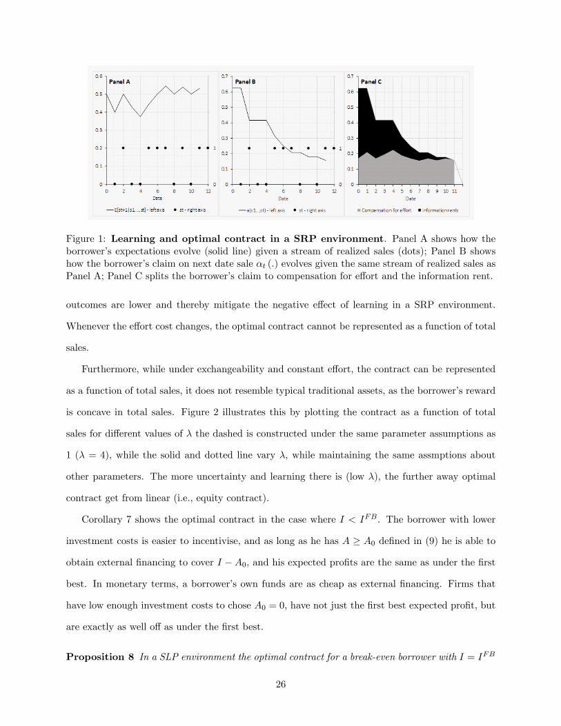
Figure 1: Learning and optimal contract in a SRP environment. Panel A shows how theborrower’s expectations evolve (solid line) given a stream of realized sales (dots); Panel B showshow the borrower’s claim on next date sale αt (.) evolves given the same stream of realized sales asPanel A; Panel C splits the borrower’s claim to compensation for effort and the information rent.
outcomes are lower and thereby mitigate the negative effect of learning in a SRP environment.
Whenever the effort cost changes, the optimal contract cannot be represented as a function of total
sales.
Furthermore, while under exchangeability and constant effort, the contract can be represented
as a function of total sales, it does not resemble typical traditional assets, as the borrower’s reward
is concave in total sales. Figure 2 illustrates this by plotting the contract as a function of total
sales for different values of λ the dashed is constructed under the same parameter assumptions as
1 (λ = 4), while the solid and dotted line vary λ, while maintaining the same assmptions about
other parameters. The more uncertainty and learning there is (low λ), the further away optimal
contract get from linear (i.e., equity contract).
Corollary 7 shows the optimal contract in the case where I < IFB. The borrower with lower
investment costs is easier to incentivise, and as long as he has A ≥ A0 defined in (9) he is able to
obtain external financing to cover I − A0, and his expected profits are the same as under the first
best. In monetary terms, a borrower’s own funds are as cheap as external financing. Firms that
have low enough investment costs to chose A0 = 0, have not just the first best expected profit, but
are exactly as well off as under the first best.
Proposition 8 In a SLP environment the optimal contract for a break-even borrower with I = IFB
26
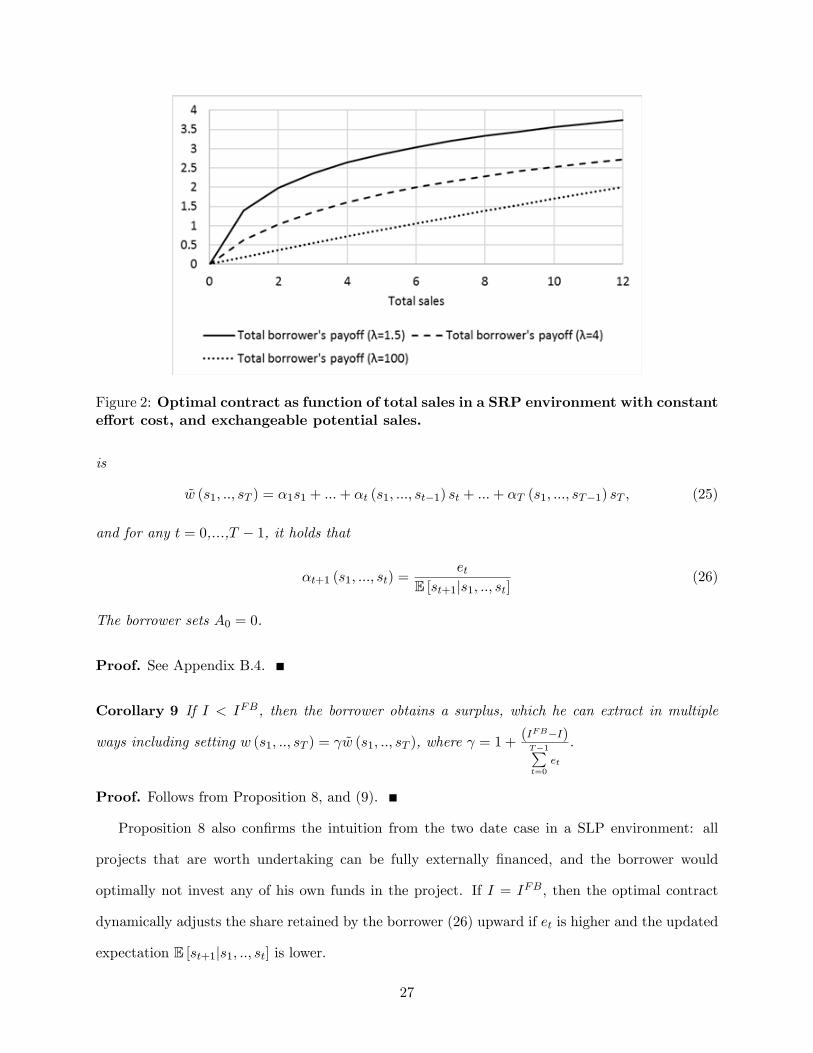
Figure 2: Optimal contract as function of total sales in a SRP environment with constanteffort cost, and exchangeable potential sales.
is
w (s1, .., sT ) = α1s1 + ...+ αt (s1, ..., st−1) st + ...+ αT (s1, ..., sT−1) sT , (25)
and for any t = 0,...,T − 1, it holds that
αt+1 (s1, ..., st) =et
E [st+1|s1, .., st](26)
The borrower sets A0 = 0.
Proof. See Appendix B.4.
Corollary 9 If I < IFB, then the borrower obtains a surplus, which he can extract in multiple
ways including setting w (s1, .., sT ) = γw (s1, .., sT ), where γ = 1 +(IFB−I)T−1∑t=0
et
.
Proof. Follows from Proposition 8, and (9).
Proposition 8 also confirms the intuition from the two date case in a SLP environment: all
projects that are worth undertaking can be fully externally financed, and the borrower would
optimally not invest any of his own funds in the project. If I = IFB, then the optimal contract
dynamically adjusts the share retained by the borrower (26) upward if et is higher and the updated
expectation E [st+1|s1, .., st] is lower.
27

Figure 3: Learning and optimal contract in a SLP environmentPanel A shows how the borrower’s expectations evolve (solid line) given a stream of realized sales(dots); Panel B shows how the borrower’s claims on next date sales αt (.) evolve given the samestream of realized sales as in Panel A.
Figure 3 gives an example of an optimal contract in SLP environment when I = IFB and
T = 12. It shows how the borrower’s expectations and αt+1 (s1, ..., st) evolve following the same
realized path of sales as in Figure 1. The figure is now constructed under the assumption that the
potential sales process is a random sampling without replacement, which is a special case of the
setting described in Section 2.1.1, where N = 30, K = 15, θ0 = 1. As before, assume that IFB = 5
and effort cost is et = e = 1/12. The borrower now revises his expectations downward following a
successful sale and upward following no sale. Furthermore, in contrast to the SRP environment, the
optimal contract in the SLP environment does not need to give the borrower’s information rents.
Because of that, the borrower claim on the next sales revenues adjusts upward and downward in
an opposite direction compared to the borrower’s expectations. The optimal contract in this case
resembles a reward scheme that gives the borrower a higher share of the next sale following a success
and a lower share following a failure.
Finally, we can see from Propositions 6 and 8 that the variables that determine the optimal
splitting rule are simple conditional expectations E [st+1|s1, .., st], and in the case of a SRP en-
vironment also a "conservative" estimates of sales at a future dates st+h, if no sales happen in
between, E [st+h|s1, .., st, st+1 = 0, ..., st+h−1 = 0]. These variables have an intuitive interpretation
and could be estimated based on the data. A "smart contract" could either be based on analyzing
28

these scenarios ex-ante or could estimate these variables on a running basis via an automated (an
preagreed) learning algorithm.
3 The role of frequent learning
3.1 Optimal contract under infrequent learning
As argued in the introduction, there is a trend towards more frequent learning and decision making.
To understand the effect of this on external financing, one needs to contrast the results under
frequent learning analyzed in Section 2 to the case where learning and possibilities to adjust effort
are less frequent.
Suppose that the contracting environment remains as described in Section 2.1, except that the
borrower observes realized cash flows only once at date T/2, and assume that T ≥ 4 is an even
number. Concequently, the borrower decides whether to make effort only at date 0 and at date
T/2. Define the cumulative potential sales as cT/2 ≡T/2∑t=1
st and cT ≡T∑t=1
st, and call the effort cost
needed to generate cT/2 and cT − cT/2 with T e02 and
T eT/22 , respectively.
Proposition 10 The optimal contract for a break-even borrower is
w(cT/2, cT − cT/2
)= αT/2cT/2 + αT
(cT/2
) (cT − cT/2
),
where
αT(cT/2
)=T eT/2
2
1
E[cT − cT/2|cT/2
]and
αT/2 =
T2
(e0−eT/2)E[cT/2]
+ αT (0)E[cT−cT/2]E[cT/2]
in SRP environmentT2
e0E[cT/2]
in SLP environment
Futhermore, the borrower chooses
A0 =T eT/2
2
E[cT − cT/2
]− E
[cT − cT/2|cT/2 = 0
]E[cT − cT/2|cT/2 = 0
] , (27)
in SRP environment and A0 = 0 in SLP environment.
Proof. See Appendix B.5.
29

Proposition 10 confirms the results in Section 2. Furthermore, note the optimal contract cannot
the generally be expressed as a function of total sales cT only. That is, even if the borrower operates
in SRP environment, the effort cost is constant (i.e., e0 = eT/2), and the potential sales distribution
is exchangeable (i.e., E[cT − cT/2
]= E
[cT/2
]), the timing of sales matters. For example, if the
borrower sells two widgets in total, he will get 2αT (0) if he sells both before T/2, but he will get
αT (0) + αT (1) < 2αT (0) if he sells one befor and one after date T/2.
Proposition 10 is mostly needed for gaining additional insights regarding the effect of increasing
frequency of learning on the optimal contracts and accessibility of extrenal financing when keeping
the total cost of effort constant. As by Propositions 8 and 10, the optimal contract in SLP envi-
ronment enables all positive NPV projects to be externally financed regardless of the frequency,
we only need to consider the SRP environment. The quantitative effects of faster learning is best
understood under specific parametric setting, so I will consider the parametric case descibed in
Section 3.1, where N = K = T , and λ is finite. Further assume that the effort cost is constant
(i.e., et = e in the frequent decisions case and e0 = eT/2 = e in the infrequent decisions case), such
that the total effort cost is fixed and equal to T e.
Corollary 11 In SRP environment described above, the break-even borrower’s own investment
under the optimal contract is
AFREQ0 = e
(T−2∑t=0
T − 1− tλ+ t
),
if he observes each sale and adjusts his effort frequently, and
AINFREQ0 = eT 2
4λ,
if he observes sales infrequently and adjusts effort only at date T/2. Furthermore, there exists a
threshold λ, such that AFREQ0 < AINFREQ0 if λ < λ, and AFREQ0 > AINFREQ0 if λ > λ.
Proof. See Appendix B.6
Corollary (11) shows that in an SRP environment, greater uncertainty about sales prospects
(lower λ) makes raising external financing more diffi cult: both AFREQ0 and AINFREQ0 are higher
when λ is lower. When there is more uncertainty there is also more learning which generates
30

greater "information rents". Interestingly, the last part of the Corollary (11) shows that when λ is
particularly low and raising external financing is most diffi cult, then the own investment required
is relatively lower under more frequent learning. This suggests that using an optimal "smart"
contract can partially mitigate these particularly negative effects of more frequent learning.
In the next section, I will contrast the effect of increasing frequency of learning under optimal
contracts to those that emerge if the borrowers where to be limited to use inflexible traditional
assets, such as equity or debt. I will also contrast the overall magnitudes of own investment under
these contracts at a given frequency of learning.
3.2 Smart-contract vs. traditional assets
To keep things comparable, I maintain here assumption that these standard contracts also benefit
from the positive features of blockchain, i.e., verification is costless and borrowers commit to the
contractual terms in date 0.17 I will focus in greater detail on debt and equity and discuss convertible
securities at the end of this section.
As payoffs under standard debt and equity depend on total sales, let us define total potential
sales and realized sales respectively as
cT =T−1∑t=0
st+1 and cT =T−1∑t=0
st+1 =T−1∑t=0
1tst+1
The standard equity contract specifies the borrower’s reward as
wE (cT ) = αE cT ,
where αE is fixed, and the standard debt contract specifies the borrower’s reward as
wD (cT ) =
{cT − d, if cT ≥ d
0, otherwise
For the sake of concreteness, I focus here on the parametric examples for both SRP and SLP
environments following the setting based on Section 2.1.1. As an example of SRP environment
I consider exactly the same case as in Section 3.1, where the borrower is not uncertain about
who the potentially interested customers are, but is uncertain about their correlated preferences17 If (realistically) traditional assets are associated with further frictions due to positive verification and enforcement
costs, then both debt and equity contracts cannot be less expensive than what is assumed here.
31

drawn from a beta distribution. In such a case cT has beta-binomial distribution with parameters
(T, λθ0, λ (1− θ0)). As an example of SLP environment, I consider the case where the borrower
knows that each potentially interested consumer will buy the product, but meets interested and
non interested consumers randombly, i.e., using the notation from section 2.1.1 T < K < N and
θ0 = 1. In such a case cT has a hypergeometric distribution with parameters (T,N, kN), where
k = KN denotes the prior mean of this distribution. Notice that the limit with λ → ∞ in the
beta-binomial distribution case and N → ∞ in the hypergeometric distribution case corresponds
to independent sales, where cT has binomial distribution Bin (T, θ0) and Bin (T, k) respectively.
Assume further that et = e0 = eT/2 = e.
Let us start by considering a break-even borrower, who has suffi cient own funds to cover in-
vestment cost I = IFB. This benchmark is helpful as we know that the borrower’s utility from the
project is maximized when he makes an effort at all dates and assuming he has enough own funds
simply guarantees that raising some external financing is possible under all contracts.
Consider then an equity contract. All incentive compatibility constraints (8) need to be sat-
isfied for the borrower to make an effort at all dates. As equity contract is linear in sales, this
requires that αEE [st+1|ct] ≥ e for any t in the frequent learning case and αEE[cT/2
]≥ e and
αEE[cT − cT/2|cT/2
]≥ e in the infrequent learning case. The least costly equity contract is the
one where the incentive compatibility constraint binds in the state where the borrower’s beliefs
about the prospects of making a next sale are at their lowest. In a SRP environment these beliefs
are at their lowest when the borrower has not made any sales until the last time he chooses effort.
This implies that the borrower’s equity share is αFREQE,SRP = e(T−1+λ)λθ0
and αINFREQE,SRP =e(T2 +λ)λθ0
in
the case of frequent and infrequent learning, respectively. Using this we find that the break-even
borrower’s own investment required is
AFREQE,SRP = e(T − 1)T
λ> AFREQ0 = e
(T−2∑t=0
T − 1− tλ+ t
)AINFREQE,SRP = e
T 2
2λ> AINFREQ0 = e
T 2
4λ,
under frequent and infrequent learning, respectively. We can see that equity requires noticeably
greater own investment from the borrower that the optimal smart contract, e.g., twice as high in
32

the case of infrequent decisions. Furthermore, as AFREQE,SRP − AINFREQE,SRP = eT (T−2)
2λ is positive and
decreasing in λ for any T > 2 and finite λ, more frequent learning makes raising equity financing
always more costly, and more so if there is more uncertainty. Recall that this is in contrast to the
optimal "smart" contract, where more frequent learning leads to a relatively lower requirement of
own financing with a suffi ciently low λ.
In a SLP environment, the borrowers’expectations about future sales prospects are at their
lowest when the borrower has made successful sales every period until he makes his last contract
relevant effort decision. This implies that αFREQE,SLP = e N−(T−1)kN−(T−1) and α
INFREQE,SLP = e
N−T2
kN−T2
, and the
break-even borrower’s own investment required is
AFREQE,SLP = eN − (T − 1)
kN − (T − 1)> 0
AFREQE,SLP = eN − T
2
kN − T2
> 0
Obtaining external financing is more diffi cult than under the optimal "smart" contract also in the
SLP environment. In particular, all positive NPV projects cannot be equity financed without the
borrowers own funds. Furthermore, the more informative past sales are about future prospect (lower
N), the more own funds are needed, and the more costly raising external financing becomes when
frequency of learning and effort decisions increases (as AFREQE,SLP −AFREQE,SLP = e (1−k)N(T−2)
2(kN−(T−1))(kN−T2 )> 0
and decreasing in N).
At the limit λ → ∞ or N → ∞, the sales are independent over time. Because effort cost is
constant, the equity contract is the optimal contract (with αE = eθ0or αE = e
k ) in the special case
of i.i.d sales. This highlights that what makes equity suboptimal in this setting is learning from
past sales. An equity contract that induces effort in all periods requires the borrower to maintain
a high share of all sales revenues in all states. This is costly because the borrower would instead
benefit from signing a "smart" contract that gives him a lower share in states where he considers the
prospect of making further sales relatively easier in order to get financing at better terms ex-ante.
Satisfying all incentive compatibility constraints (8) under a simple debt contract is even harder.
The borrower owes a fixed amount, which implies that his effort incentives are at their lowest when
he has not managed to sell any widgets until the last date he makes an effort decision. The
33

consequences of this are particularly stark, in the frequent learning and decisions case as no debt
contract with a face value d ≥ 1 can incentivize the borrower to make an effort at date T − 1
when cT−1 = 0. This implies that the probability of making just one sale at the last date must be
suffi cient to cover d, and the maximum face value of debt must therefore satisfy
Pr (sT − d ≥ 0|cT−1 = 0)E [sT − d|cT−1 = 0, sT − d ≥ 0] = e
As sT − d ≥ 0 only if sT = 1, this simplifies to
d = 1− e
Pr (sT = 1|cT−1 = 0).
We obtain the required borrower’s own investment from the lender’s break-even constraint as
AD = IFB − d (1− Pr (cT = 0)) ,
where IFB = E [cT ] − T e. As the term d (1− Pr (cT = 0)) is small, it follows that a break even
investor would need to largely self-finance the break-even project to be able to undertake it.
Using the specificified distributional assumptions, we can also find that d is given by
dFREQSRP = 1− eλ+ T − 1
λθ0
dFREQSLP = 1− eN − (T − 1)
kN,
in a SRP and SLP environment, respectively. The firm’s ability to raise debt financing is limited
in both cases, as well as in the case of independent sales (when λ → ∞, or N → ∞). When
there is more uncertainty, the borrower can raise even less debt in a SRP environment as dFREQSRP
is increasing in λ. Not only does the borrower need to have a low enough debt burden to have an
incentive to continue after not selling, his expectations about the prospects of selling a widget at
the last data are particularly low because of learning. There is an opposite learning effect in a SLP
environment and dFREQSLP is higher when there is more learning (lower N).
Figure 4 compares the own funds the break-even investor needs to contribute to pursue his
project under different financing contracts, and the frequencies of learning and decision making.
It considers the same parameter values as in Section 2.3.1.18 As T = 12, we can refer to the full18That is T = 12, IFB = 5, e = 1/12. The SLP environment further assumes θ0 = 0.5, λ = 4 and N = K = 12.
The i.i.d. environment assmes probability of selling at any period is always 0.5, and SLP environment assmes θ0 = 1,N = 30 and K = 15, such that k = 0.5.
34

Figure 4: Borrowers own funds needed for first best effort under different contracts and learningenvironments.
period as "a year", so that there is one selling opportunity each month. The frequent learning and
effort decision are the "monthly" decisions, and infrequent decisions take place in at the start of
"Janury" and "July" only.
We can see that traditional assets indeed require noticeably higher own investment by the
borrower compared to the optimal contract. This gap widens when the frequency increases (black
bars reflect frequent learning and grey bars reflect infrequent learning). Furthermore, debt is more
expensive that equity. These main observations are not specific to the choice of parameters.
It was assumed up to now that the borrower has enough own funds and simply prefers not to use
these (because of lexicographic preferences). When I < IFB, then the above results also indicate
the maximum investment a borrower with no own funds can undertake while still obtaining the the
same expected profits as under the first best. Such maximum investment cost can be calculated
by subtracting the values reported on Figure 4 from IFB = 5. For example, in a SRP environment
with frequent decisions, investment costs up to 5 − 0.63 = 4.37 can be always covered via the
optimal contract, while investment costs up to only 5 − 2.75 = 2.25 and 5 − 4.64 = 0.36 can be
covered via equity and debt contract, respectively.
Borrowers that have higher investment costs can still get financing via debt or equity, but
financing in such a case must always be costlier for them, which in turn reduces their expected
utility from the project. Consider the example of a debt contract. If a debt contract with face
35

value d ≥ 1 is feasible, then the borrower and the lender both expect that the borrower will quit
making an effort after observing some suffi ciently bad sales history. Because the realized sales cT
is a sum that is increasing in effort decisions, it follows that the distribution on realized sales cT
would be first order stochastically dominated by the distribution of cT , hence the expected value of
the project would be lower. It is then immediate from the lender’s break even constraint (2) that at
any given wealth of the borrower and investment cost, the reward that the borrower receives is also
lower, which reduces the borrower’s expected returns. It then follows that there exists a threshold
investment level, lower than the one under the optimal contract, above which debt financing is
impossible. A similar argument applies to equity contracts.
Figure 5: Distribution of realized sales cT , under a debt contract and endogenous effort choices atdifferent frequencies.
To illustrate it further, consider a borrower with no own funds, i.e., A = 0, T = 12 and e = 1/12
and with a project that can generate i.i.d. potential sales, each with probability 0.5. Figure 5 plots
the distribution of total realized sales, cT , under the highest investment cost that can be debt
financed. If there is just one effort choice at the beginning of "January", then Modigliani and
Miller results remain applicable and the highest first best investment I = 5 can be debt financed
(the resulting realized sales distribution is binomial and represented by the light grey bars). When
the borrower can adjust his effort in "July", the highest investment cost that can be debt financed
is I = 4.96. Under this contract the borrower will optimally stop making efforts if he has not sold
36

at least one widget during the first half of the year. The resulting realized sales distribution is
stochastically worse as the low outcomes are more likely (darker grey bars). When the borrower
makes effort decisions frequently then the realized sales distribution becomes ever more shifted
towards the low outcomes (black bars), and the highest investment cost that can be covered is
I = 4.42. Due to more frequent learning and effort decisions, the borrower is more likely to quit
and stop making efforts if he does not achieve the following benchmarks: 1) at least one successful
sale by date 4; 2) at least two successful sales by date 6; 3) at least three successful sales by date
8 and 4) at least four successful sales by date 10. Furthermore, a discount bond that covers the
investment cost under these three cases has an increasingly high discount rate when the frequency
increases: 9.0%, 9.9% and 23.8% under "January" only, "January" and "July", and "monthly"
decison frequences.
Overall these results highlight that more frequent of learning and decisions makes financing via
traditional assets more diffi cult for the borrowers. As the relative benefits of the "smart" contracts
derived in this paper become higher when the learning and effort decisions are more frequent, it
suggests that an important benefit of the new technological possibility enabled by hashlinked and
timestamped record keeping and the associated possibility to write frequently adjusting "smart"
contracts is that these contracts mitigate the negative effects that the trend towards better and
faster learning technologies has on the accessibility of external financing. This is particularly
important when past sales data provide more information about future prospects.
Finally, the contract under infrequent decision making could indeed be viewed as a convertible
asset. Indeed start-ups sometimes also raise financing via convertible assets (such as preferred
shares used by venture capitalist). Nevertheless, in a SRP environment the optimal convertible
asset in this setting adjusts in an opposite direction compared the preferred shares used in venture
capital context. This is not surprising as venture capitalists are argued to use preferred shares
primarily to safeguard their investment against the entrepreneur misusing or diverting the initial
funds invested, e.g., by selling the firm too early (see e.g., Lerner et. al. 2012). This friction is not
present in my setting as it could at least theoretically be eliminated via the so called "conditional
payments" that can be built in "smart" contracts based on the same technology. Such code can
37

delegate the agreed investment to an escrow account and be pre-programmed to release these only
"conditional" on a proof of pre-agreed use. For example, it could effectively disallow the initial
owner to sell the firm or product line before a given moment in time by making the new owner’s
claims on future sales equal to zero. While a typical venture capital contract would adjust is the
"right" direction in SLP environment, it may be less relevant in a venture capital context if one
considers that these firms often target firms with large potential for positive network effects, which
as discussed in Section 2.1.1 is a characteric of a SLP environment.
The two period case aside, commonly used convertible securities do not convert arbitrarily
frequently. With high enough T and rich enough statistical dependencies between potential sales,
one cannot express the "smart" contract derived as a combination of traditional securities.
4 Conclusion
This paper explored how the blockchain environment could change the borrower-lender relationship.
Blockchain brings effi ciency gains such as costless verification and automatic enforcement, and all
possible financing contracts would benefit from these gains. At the same time, the blockchain
technology is emerging in an environment where agents can learn from their cash flow data (due
to for example advances in computer power and big data analytics), update their beliefs about
future prospects and make decisions faster. If anything, blockchain is likely to facilitate such faster
learning and decision making.
I show that an ideal borrowing contract in this environment would be an automatically adjust-
ing profit sharing agreement, and for this reason reliable timestamps of records is an important
feature of blockchain records. How the optimal contract should adjust depends on the fundamental
characteristics of the market where the firm is selling its products. Dynamics differ depending on
whether the firm operates in a market where better than expected sales outcomes are associated
with expected higher future demand or lower future demand. With such a contract, agents are able
to test out their ideas with minimal need for own funds, and the economic outcomes are closer to
those of a frictionless market.
An environment with frequent decisions is particularly bad for standard debt contracts because
38

it gives poor incentives for the borrower to make effort after unlucky outcomes. If one were to be
restricted to use only debt and simple equity contracts, then equity would dominate debt contracts.
When compared to the optimal contract, the equity contract is almost as good when sales do not
reveal a lot of new information, and noticeably worse if sales data are very informative about future
prospects. Equity contracts also do not optimally adjust to the dynamics of effort cost.
It can be argued that even without blockchain, debt contracts could become worse in the
future, given that there is a trend towards shorter contracts, and improving capabilities for faster
data analysis and decision making. If the negative effects of frequent decision making are foreseen
by lenders, it can make debt contracts more expensive for borrowers, and if not foreseen, it could
increase the frequency of defaults. Perhaps the most compelling reason for using debt contracts has
been the costs associated with verifying cash flow and optimizing monitoring efforts. As verification
costs are becoming smaller, it could encourage the creation of new types of financing contracts that
are "equity-like" and ideally more flexible than equity; the recent emergence and success of equity
crowdfunding and initial coin offerings seems to be a movement in this direction.
My setting assumes that there is no information asymmetry at the time of contracting and the
potential sales distribution is known to both parties. One would obtain the same results if the
borrower and lender agreed on how the borrower’s incentives are likely to change following realized
sales, even if the prior joint probability distribution is subjective. It is also plausible that the
borrower could have superior information about his target market at the time of contracting. While
this could lead to additional diffi culties, there are other contemporary developments that would
enable the contracting parties to mitigate this information asymmetry before contracting, e.g.,
reward-based crowdfunding, which can be used to test the market and produce public information
about the preferences of target consumers (see e.g., Chemla and Tinn 2017).
More broadly this paper contributes to the financial contracting literature by highlighting the
effects of frequent learning and decision making on incentives, and characterizes how these effects
depend on general distributional properties. I showed that in a realistic environment where bor-
rowers’effort choices are dynamic, the sequence of cash flow arrivals is important and this explains
why my findings are in contrast to some influential existing papers on this topic.
39

My analysis suggests that the more important benefit of blockchain and "smart" financing
contracts could be the possibility to design new, more flexible, types of contracts rather than the
possibility to manage and seize collateral more easily, an argument often emphasized in this context.
My model shows that there is less need for own investment and collateral under the optimal self-
adjusting contract, which makes external financing noticeably more accessible.
40

Appendix
A Further background on blockchain technology
A blockchain, or more precisely a hash-linked and timestamped ledger, is a database where dig-
ital data is recorded in chronological timestamped blocks that are cryptographically linked via a
hash function. Hash functions are one way functions that take an input (numerical and/or textual
data) and return a fixed-size alphanumeric string. The main feature of any good cryptographic
hash function is that it is easy to calculate the correct hash from the given data and computa-
tionally extremely diffi cult to reconstruct the original input from a given hash. A hash-linked and
timestamped ledger further imposes a chronological structure, where the hash reflecting the state
of agreed records at some point in time is included to the next record. For cryptographic integrity,
the main benefit of this structure is that it becomes increasingly diffi cult to alter historical records.
When considering financial contracting, data recorded on such ledger could be detailed accounting
data, ownership data, terms of a financing contract, as well as a code for implementing pre-agreed
contractual terms.
While the precise origin and definition of the term "blockchain" itself is subject to some disagree-
ments, hash-linked timestamping is a common feature behind all forms of blockchain technology.
The idea that hash-linked timestamping can be used to create secure digital records which provide a
reliable digital proof when these records where generated was first proposed in computer science by
Haber and Stornetta (1991, 1997). This idea has lead to both further research and prominent real
world applications. It is well known that Nakamoto (2008) combined this idea with a proposal of a
proof-of-work verification system to propose Bitcoin, digital money created outside the control of
traditional public and private institutions. It is perhaps less known that in 2007 Guardtime built on
hash-linked timestamping to launch a formally verifiable security system for the Estonian Govern-
ment, which also eliminates third parties, trusted insiders or cryptographic keys in the verification
of the integrity of government records, networks and systems. Guardtime was built on research
by Buldas, Laud, Lipmaa, and Villemson (1998), and Buldas and Saarepera (2004) who provided
41

a formal proof of the idea of time-stamping proposed by Haber and Stornetta.19 Nowadays there
are many forms of blockchain initiatives that broadly fall under two categories: those that rely on
permissionless verification systems as Bitcoin (most notable of those is the Ethereum project that
enables smart contract functionality based on a Ethereum coin), and those that rely on permis-
sioned verifications systems in the spirit of Guardtime (most notable of those is the Hyperledger
project - a consortium of well-known technology platform companies, financial services and Busi-
ness Software companies)20 While verification systems differ, all blockchains rely on hash-linked
timestamping. The particular verification mechanism is not of primary importance for the mech-
anisms in this paper. Permissioned systems do not require for example costly mining to record a
block of transactions, are more scaleable and can maintain privacy more easily, while permissionless
systems are more decentralized as any member of public can participate in validating new blocks.
The extent of decentralization in permissioned systems depends upon the number of peers, the
expected number of bad nodes in the network, and the type of consensus mechanism the members
agree to.
The term "smart contracts" was highlighted by Szabo (1994, 1997) as a tool that enables the
automatic execution of contracts, lowers enforcement costs and minimizes the need for interme-
diaries. Werback and Cornell (2017) emphasise that from a legal perspective the distinct feature
of "smart contracts" is that the burden of proof is reversed - a pre-agreed contract would first be
automatically executed and disputes about the fairness of the contracts could happen later. In my
setting, this effectively safeguards the lender by eliminating enforcement costs and makes it eas-
ier/cheaper to contract for the borrower (see also Rius (2018) for the analyses of Ethereum based
"smart contracts" from a computer science perspective).21
19Buldas and Saarepera are further associated with a number of patents assigned to Guardtime See e.g., patentsgranted to Guardtime US8719576B2 (2003) "Document verification with distributed calendar infrastructure" thatrefers to timestamping; US9853819B2 (2013) "Blockchain-supported, node ID-augmented digital record signaturemethod" that refers to timestamping and blockchain. The company now also provides blockchain based digitalsecurity services for DARPA, and Erisson, among others20 Including technology firms (Cisco, Fujitsu, Hitachi, IBM, Intel, NEC, NTT DATA, Red Hat, VMware), financial
services firms (ABN AMRO, ANZ Bank, BNY Mellon, CLS Group, CME Group, the Depository Trust & ClearingCorporation (DTCC), Deutsche Börse Group, J.P. Morgan, State Street, SWIFT, Wells Fargo), Business Softwarecompanies like SAP, Systems integrators and others such as: (Accenture, Calastone, Wipro, Credits, Guardtime,IntellectEU, Nxt Foundation, Symbiont).21For example, Blockchain-based records and smart contracts are often referred to as immutable, because the records
are verifiable and a code implementing a smart contract can be recorded on the blockchain as well. Immutability is
42
B Proofs
B.1 Parametric example of SRP vs. SLP in two period case
Consider a parametric setting described in Section 2.1.1 and two first sales at t = 1, 2. By the law
of total expectations, the joint distribution
p (s1, s2) = Pr (τ1 = NI, τ2 = NI) p (s1, s2|τ1 = NI, τ2 = NI)
+ Pr (τ1 = NI, τ2 = PI) p (s1, s2|τ1 = NI, τ2 = PI)
+ Pr (τ1 = PI, τ2 = NI) p (s1, s2|τ1 = PI, τ2 = NI)
+ Pr (τ1 = PI, τ2 = PI) p (s1, s2|τ1 = PI, τ2 = PI) ,
where the probabilities of meeting different consumer types are Pr (τ1 = NI, τ2 = NI) = N−KN
N−1−KN−1 ,
Pr (τ1 = NI, τ2 = PI) = Pr (τ1 = PI, τ2 = NI) = N−KN
KN−1 and Pr (τ1 = PI, τ2 = PI) = K
NK−1N−1 .
Note also that the probability of making a positive sale to a type "NI" consumer is impossible,
hence for example p (s1, s2|τ1 = NI, τ2 = NI) = 0 whenever s1 = 1 or s2 = 1,
p (s1 = 0, s2 = 1|τ1 = PI, τ2 = NI) = 0, etc. Furthermore, meeting a type "NI" reveals no infor-
mation about θ, and thus for example p (s1 = 0, s2 = 1|τ1 = NI, τ2 = PI) = p (s2 = 1|τ2 = PI) =
E [p (s2 = 1|θ, τ2 = PI) |τ2 = PI] = E [θ] = θ0.
At the same time, meeting two type "PI" consumers reveals information about θ, as by the law
of iterated expectations and the expression for p.d.f. of beta distribution, we find that
p (s1, s2|τ1 = PI, τ2 = PI) = E [s1, s2|θ, τ1 = PI, τ2 = PI]
= E[θs1+s2 (1− θ)1−(s1+s2)
]=
∫ 1
0
θs1+s2 (1− θ)2−(s1+s2) θλθ0−1 (1− θ)λ(1−θ0)−1 dθ
B (λθ0, λ (1− θ0))
=B (λθ0 + s1 + s2, λ (1− θ0) + 2− (s1 + s2))
B (λθ0, λ (1− θ0)),
where B (x, y) is a beta function for Rex > 0 and Re y > 0. Using further that beta function can
be expressed via gamma functions Γ (.) as B (x, y) = Γ(x)Γ(y)Γ(x+y) , and gamma function satisfies the
not absolute, as a transaction or a rule can be "un-done" by a new rule. Yet, unilateral "un-doing" of a transactionis likely to be very costly and rare from a perspective of small participants such as financiers and entrepreneurs inmy setting, unless there is a major issue of non-legitimate behaviour. There was a well known case of a major caseof users exploiting a vulnerability of DAO that lead to a modification of Ethereum blockchain, effectively restoringthe pre-attack state.
43

recurrence relation Γ (x+ 1) = xΓ (x), we find that
p (s1 = 0, s2 = 0|τ1 = PI, τ2 = PI) =λ (1− θ0) (λ (1− θ0) + 1)
λ (λ+ 1)
p (s1 = 0, s2 = 1|τ1 = PI, τ2 = PI) =λθ0λ (1− θ0)
λ (λ+ 1)
p (s1 = 1, s2 = 0|τ1 = PI, τ2 = PI) =λθ0λ (1− θ0)
λ (λ+ 1)
p (s1 = 1, s2 = 1|τ1 = PI, τ2 = PI) =λθ0 (λθ0 + 1)
λ (λ+ 1).
From all this, we can specify the joint distribution of sales as
p (s1 = 0, s2 = 0) =N −KN
N − 1−KN − 1
+ 2N −KN
K
N − 1(1− θ0)
+K
N
K − 1
N − 1
λ (1− θ0) (λ (1− θ0) + 1)
λ (λ+ 1)
p (s1 = 0, s2 = 1) =N −KN
K
N − 1θ0 +
K
N
K − 1
N − 1
λθ0λ (1− θ0)
λ (λ+ 1)
p (s1 = 1, s2 = 0) =N −KN
K
N − 1θ0 +
K
N
K − 1
N − 1
λθ0λ (1− θ0)
λ (λ+ 1)
p (s1 = 1, s2 = 1) =K
N
K − 1
N − 1
λθ0 (λθ0 + 1)
λ (λ+ 1)
In the two period case stochastic affi liation is equivalent to comparing conditional probabilities as
p (s1 = 0, s2 = 0) p (s1 = 1, s2 = 1) ≥ p (s1 = 0, s2 = 1) p (s1 = 1, s2 = 0)⇐⇒p (s1 = 0, s2 = 0)
p (s1 = 0, s2 = 1)≥ p (s1 = 1, s2 = 0)
p (s1 = 1, s2 = 1)⇐⇒
1 +p (s1 = 0, s2 = 0)
p (s1 = 0, s2 = 1)≥ 1 +
p (s1 = 1, s2 = 0)
p (s1 = 1, s2 = 1)⇐⇒
p (s1 = 0)
p (s1 = 0, s2 = 1)≥ p (s1 = 1)
p (s1 = 1, s2 = 1)⇐⇒
Pr (s2 = 1|s1 = 1) ≥ Pr (s2 = 1|s1 = 0) .
Using the expressions above, we find that p (s1 = 0) = N−KN + K
N (1− θ0), p (s1 = 1) = KN θ0, and
Pr (s2 = 1|s1 = 1) =K − 1
N − 1
λθ0 + 1
λ+ 1
Pr (s2 = 1|s1 = 0) =N −KN − 1
Kθ0
N −K +K (1− θ0)+K − 1
N − 1
Kλθ0 (1− θ0)
(λ+ 1) (N −K +K (1− θ0))
From here we obtain that Pr (s2 = 1|s1 = 1) ≥ Pr (s2 = 1|s1 = 0) if, and only if,
λθ0 (N −K) ≤ N (K − 1)− θ0K (N − 1) .
44

First, notice that this inequality always holds when K = N , as left hand side becomes zero and
the right hand side becomes N (N − 1) (1− θ0) ≥ 0. Second, provided that N > K, we obtain
that this inequality never holds if θ0 >N(K−1)K(N−1) . Note that such values for prior mean always exist
as N(K−1)K(N−1) < 1. Denoting the share of potentially interested consumers with k ≡ K
N , we can write
N(K−1)K(N−1) = Nk−1
k(N−1) , which is increasing in N and k. Hence the condition θ0 >N(K−1)K(N−1) is less likely
to hold when θ0 is lower, and N and k are higher. Third, when N > K and θ0 ≤ N(K−1)K(N−1) , then
there exists a cutoff value of λ, such that sales are stochastically affi liated if, and only if,
λ ≤ λ =N (K − 1)− θ0K (N − 1)
θ0 (N −K)=
(Nk − 1)− θ0k (N − 1)
θ0 (1− k).
As ∂λ∂θ0
< 0, ∂λ∂N > 0 and ∂λ
∂k > 0, also this condition is more likely to hold when θ0 is lower, and N
and k are higher. As with two periods the random variable can only be affi liated of not, higher λ
and θ0, and lower N and k imply a SLP environment.
B.2 Proof of Lemma 3
Proof of Part 1) of Lemma 3. The value of the project
π =T−1∑t=0
(1tst+1 − 1tet)− I, (28)
Let us establish that setting 1t = 1 for all t is optimal, and thus πFB =T−1∑t=0
(st+1 − et)−I. Suppose
instead that the borrower makes no effort at some date τ . Then value of the project under such
deviating strategy is
π′ =τ−1∑t=0
(st+1 − et) +T−1∑t=τ+1
(st+1 − et)− I,
From here πFB − π′ = sτ+1− eτ , and E[πFB − π′
]= E [sτ+1]− eτ . As the effort cost was assumed
to be small, i.e., eτ ≤ E [sτ+1|10s1, ..., 1t−1st, 10, .., 1t−1], it follows that E [sτ+1] ≥ eτ , and such
deviation is not profitable. Under 1t = 1,
E[πFB
]=
T−1∑t=0
E [st+1]−T−1∑t=0
et − I.
Proof of Part 2) of Lemma 3. Consider then the contracting problem (1)-(3). Replacing
the lender’s break even constraint (2) in the borrower’s utility (1), we obtain that the borrower’s
45

expected utility from the project at date 0 is
E [π] = E[T−1∑t=0
1tst+1 − 1tet]− I, (29)
which cannot be higher than E[πFB
]above, and is achieved by setting 1t = 1 for all t. Notice that
A0 does not enter in (29), and thus under 1t = 1, all contracts are equivalent and maximize the
borrower’s primary objective. By the borrower’s secondary objective, the optimal contract must
then set own investment, A0, to a lowest feasible value. Furthermore, setting 1t = 0 for some t
cannot lead to a lower A0. To see this, suppose that there exists a feasible contract with A′0 and
w′ (s1, ...,sT ), which has 1t = 0 for some t, and gives expected profit E[πFB
]. To give the borrower
expected profit E[πFB
], by (1) it must be the case that
A′0 = E[w′ (s1, ...,sT )
]− E
[πFB
]−T−1∑t=0
1tet =
= E[w′ (s1, ...,sT )
]+ I − E
[T−1∑t=0
st+1
]−T−1∑t=0
(1t − 1) et
Any feasible contract must guarantee that the lender breaks even or makes a profit, hence the own
investment from the lender’s perspective must have
A0 ≥ I − E[T−1∑t=0
1tst+1
]+ E
[w′ (s1, ...,sT )
]We then obtain
A0 ≥ A′0 +T−1∑t=0
(1− 1t) (E [st+1]− et)
where E [st+1] ≥ et implies that the termT−1∑t=0
(1− 1t) (E [st+1]− et) ≥ 0 (and can be positive) when
1t = 0 for some t, and is zero if 1t = 1 for some t.
B.3 Proof of Proposition 4
Let W ′ =[w (0, 0) w (0, 1) w (1, 0) w (1, 1)
]be the vector of the borrower’s payoffs, P ′ =[
p (0, 0) p (0, 1) p (1, 0) p (1, 1)]be the vector of associated probabilities, and
b′ =[e0 + e1 e0 e1 e1
]be the right hand side of constraints. Defining also a matrix of
46

coeffi cients
G =
p (0, 0) −p (1, 0) −p(0,1)
p1(0) 0
p (0, 1) −p (1, 1) p(0,1)p1(0) 0
p (1, 0) p (1, 0) 0 −p(1,1)p1(1)
p (1, 1) p (1, 1) 0 p(1,1)p1(1)
we can express the primal problem (11)-(13) as
minE [w (s1, s2)] = W ′P , subject to W ′G ≥ b,W ≥ 0 (30)
Defining the vector X ′ =[xp x0 x0
1 x11
]as corresponding shadow prices of constraints (12)-
(13), i.e., xp corresponds to the participation constraint, x0 to date 0 effort incentive compatibility
constraint and xs11 to date 1 effort incentive compatibility constraint when date 1 sale outcome is
s1, there is a dual maximum problem
maxV = b′X, subject to GX ≤ P,X ≥ 0. (31)
The primal and dual are linked via the Duality Theorem (Theorem 5.1 in Chvátal, 1983) and if one
has a solution, then so does the other one, and values are the same.
Let us solve the dual maximum problem. The dual maximum problem simplifies to
maxV = e0 (xp + x0) + e1
(x0
1 + x11 + xp
), (32)
subject to
xp ≤ 1; (33)
xp + x0 ≤ 1;
x01 ≤ p1 (0) (1− xp) +
p (1, 1) p1 (0)
p (0, 1)x0;
x11 ≤ p1 (1) (1− xp − x0) ;
xp, x0, x01, x
11 ≥ 0
Because the objective function (32) is increasing in x01 and x
11, the third and the fourth inequalities
in (33) must be binding. Using this in (32), the problem simplifies to
maxV = e0 (xp + x0) + e1
(xp + (1− xp) + x0p1 (0)
(p (1, 1)
p (0, 1)− p1 (1)
p1 (0)
))(34)
= e0 (xp + x0) + e1 + e1x0p (1, 1) p (0, 0)− p (1, 0) p (0, 1)
p (0, 1),
47

subject to xp ≤ 1, xp + x0 ≤ 1, xp, x0 ≥ 0. It then follows that the sign of p (1, 1) p (0, 0) −
p (1, 0) p (0, 1) determines the maximizing values of x0 and xp, and hence also the maximizing
values of x01 and x
11.
If p (1, 1) p (0, 0) > p (0, 1) p (1, 0) then from (34) the solution of the dual maximum problem is
xp = 0, x0 = 1, x01 = p1 (0)
(1 + p(1,1)
p(0,1)
), x1
1 = 0, and the maximized value is
V = e0 + e1 + e1p (1, 1) p (0, 0)− p (0, 1) p (1, 0)
p (0, 1)
Given this solution, complementary slackness (see e.g., Theorem 5.3 in Chvátal, 1983) then implies
that w (0, 0) = 0, the participation constraint need not be binding and the first two incentive
compatibility constraints in (3) must be binding. This, and the observation that the objective
function of primal problem (30) is minimized when w (1, 1) is at its lowest value, implies that all
incentive compatibility constraints are binding under the optimal solution. Solving that system
gives (14). Plugging this solution in the objective function of the primal minimization problem
(30) verifies that E [w (s1, s2)] = V , as implied by the Duality Theorem.
If p (1, 1) p (0, 0) < p (0, 1) p (1, 0) then from (34) xp = 1, x0 = 0, x01 = 0, and x1
1 = 0, and the
value
V = e0 + e1
Complementary slackness now implies that w (0, 0) = 0, the participation constraint must be bind-
ing, and incentive compatibility constraints do not need to be binding. The Duality Theorem in
that case further implies that E [w (s1, s2)] = V , which can be confirmed by plugging the solution
(16) in the primal minimization problem. Note that there can be other optimal solutions of the
primal maximum problem, but the presented solution is the only one that holds for any values of
e0, e1 ≥ 0, which satisfy 10.
If p (1, 1) p (0, 0) = p (0, 1) p (1, 0), then the two contracts are equivalent.22 This proves the
optimality of the solution in Proposition 4.
22 It is suffi cient to show that if p (1, 1) p (0, 0) = p (0, 1) p (1, 0) , then w (1, 0) in Part 1) and 2) of Proposition 4.
Indeed, we obtain that e0−e1p1(1)
+ e1p1(0)p(0,1)
p2(1)p1(1)
= e0p1(1)
+ e1p1(1)
(p1(0)p(0,1)
p2 (1)− 1)
= e0p1(1)
+ e1p1(1)
(p(0,0)p(0,1)
p2 (1)− p2 (0))
= e0p1(1)
+ e1p2(1)p1(1)
(p(0,0)p(0,1)
− p2(0)p2(1)
)= e0
p1(1)+ e1p2(1)
p1(1)
(p(0,0)p(0,1)
− p(0,0)+p(1,0)p(0,1)+p(1,1)
)= e0
p1(1)+ e1
p1(1)
(p(0,0)p(1,1)−p(1,0)p(0,1)
p(0,1)
)=
e0p1(1)
.
48

B.4 Proof of Propositions 6 and 8
The solution of the two date problem, suggests that solution of the primal minimization problem,
given by (7) and (3), takes the form described in the propositions 6 and 8. In order to prove
optimality, we again benefit from the duality and complementary slackness theorems. Denote xp
the shadow price of the participation constraint, and xs1,..,stt the shadow price of the incentive
compatibility constraint following realization history s1, .., st. The dual maximization problem is
maxV = xpT−1∑t=0
et + e0x0 + ...+ et1∑
s1=0...
1∑st=0
xs1,..,stt + ...+ eT−1
1∑s1=0
...1∑
sT−1=0xs1,..,sTT−1
subject to
p (s1, ..., sT )xp + (−1)1−s1 p (1, s2, ..., sT )x0 + ...+ (35)
(−1)1−st p (s1, ..., st−1, 1, st+1, ..., sT )
p (s1, ..., st−1)xs1,..,st−1t−1 + ...+
(−1)1−sT p (s1, ..., sT−1, 1)
p (s1, .., sT−1)xs1,..,sT−1T−1 ≤ p (s1, ..., sT )
and the non-negativity constraints xs1,..,stt ≥ 0 for every t = 1, ..., T − 1.
By Theorem 5.1-5.3 in Chvátal (1983) the proof that the solutions in Propositions 6 and 8 are
optimal requires checking that these solutions are feasible, using then complementary slackness and
confirming that the implied solution of the dual maximum is feasible as well.
Proof of Proposition 6.
Step 1) Proof that the primal guess is feasible. First, we can prove by induction that all incentive
compatibility constraints hold with equality under the guessed solution. It is clear that this is true
if t = T − 1: using (19) in (8) gives
E[
eT−1sTE[sT |s1,..,sT−1] |s1, .., sT−1
]= eT−1. Suppose then that the incentive compatibility constraint holds
with equality at some period t+ 1, i.e.,
E [w (s1, .., st+1, st+2, st+3,..., sT )− w (s1, .., st+1, 0, st+3,..., sT ) |s1, .., st+1] = et+1. (36)
49

It then follows that at t
E [w (s1, .., st, st+1, st+2,..., sT )− w (s1, .., st, 0, st+2,..., sT ) |s1, .., st]
= E [E [w (s1, .., st, st+1, st+2,..., sT )− w (s1, .., st, 0, st+2,..., sT ) |s1, .., st+1] |s1, .., st]
= E [w (s1, .., st+1, 0, st+3,..., sT ) |s1, .., st] + et+1 − E [w (s1, .., st, 0, st+2,..., sT ) |s1, .., st]
= αt+1 (s1, ..., st)E [st+1|s1, .., st]− αt+2 (s1, ..., st, 0)E [st+2|s1, .., st] + et+1 +
E [(αt+3 (s1, ..., st, st+1, 0)− αt+2 (s1, ..., st, 0, st+2)) st+3|s1, .., st] + ...+
E [(αT (s1, ..., st+1, 0, st+3, ..., sT−1)− αT (s1, ..., st, 0, st+2, ..., sT−1)) sT |s1, .., st]
= αt+1 (s1, ..., st)E [st+1|s1, .., st]− αt+2 (s1, ..., st, 0)E [st+2|s1, .., st] + et+1 = et
where the first equality follows from the law of iterated expectations, the second equality uses
(36), the third equality uses (19), the fourth follows from exchangeability, which implies that
αt+h (s1, ..., st, st+1, 0, st+3, ..., st+h−1) =
αt+h (s1, ..., st, 0, st+2, st+3, ..., st+h−1) for any h = 3, ..., T − t − 1, and the fifth follows from (20)
and exchangeability, which implies that E [st+1|s1, .., st] = E [st+2|s1, .., st]. This proves that all in-
centive compatibility constraints are binding under the guessed solution of the primal minimization
problem.
In order to confirm that the participation constraint (7) holds, note that ∆t (s1, .., st), defined in
(23), is non-negative as∆t (s1, .., st) ≥ 0 if E [st+2|s1, .., st] ≥ E [st+2|s1, .., st, 0]⇔ E [st+2|s1, .., st, 0] ≤
E [st+2|s1, .., st, 1]. The latter holds because
p (s1, .., st, 0, 1)
p (s1, .., st, 0)≤ p (s1, .., st, 1, 1)
p (s1, .., st, 1)⇔
p (s1, .., st, 0, 0) p (s1, .., st, 1, 1) ≥ p (s1, .., st, 1, 0) p (s1, .., st, 0, 1)
and the SRP environment assumes stochastic affi liation. Furthermore, the inequality is strict unless
potential sales are i.i.d. It then follows from (19), (20) and the definitions (22) and (23) that the
participation constraint holds, and is not-binding (unless potential sales are i.i.d).
Step 2) Proof of optimality. Given the results in step 1, complementary slackness implies that
xp = 0 (as the participation constraint is not binding) and constraints (35) must hold with equality
50

whenever at least one st 6= 0 (as w (s1, .., sT ) > 0 for all sequences of s1, ..., sT except the sequence
of zeros only).
To prove optimality, we need to that the solution of the dual maximization problem under these
constraints is non-negative. To shorten the notation, define zt (s1, ..., st) ≡ xs1,..,stt
p(s1,...,st), which has the
same sign as xs1,..,stt . Hence it needs to be proven that zt (s1, ..., st) ≥ 0 for any t = 0, ..., T − 1. We
already know from Proposition 4 that it T = 2 then there is a feasible solution of the dual problem,
and we can extend the proof to T > 2 by induction.
Suppose that there exists a feasible solution z0, z1 (s1) , ..., zτ−1 (s1, ..., sτ−1) ≥ 0 when T = τ ,
which satisfies the complementary slackness conditions, i.e., for all t = 0, ..., τ − 1 it holds that
(−1)1−s1 p (1, s2, ..., sτ ) z0 + ...+ (37)
(−1)1−st p (s1, ..., st−1, 1, st+1, ..., sτ ) zt−1 (s1, ..., st−1) + ...+
(−1)1−sτ p (s1, s2, ..., sτ−1, 1) zτ−1 (s1, ..., sτ−1) ≤ (=) p (s1, s2, ..., sτ ) ,
where the weak inequality holds for any st and the equality holds whenever at least one st 6= 0.
To prove optimality, it must then follow that there also exists a feasible solution zτ (s1, ..., sτ ) ≥ 0
when T = τ + 1. As by complementary slackness, it then follows that the equivalent to (37) holds
when T = τ + 1 and as sτ+1 = {0, 1}, we must show that
(−1)1−s1 p (1, s2, ..., sτ , 0) z0 + ...+ (38)
(−1)1−sτ p (s1, s2, ..., sτ−1, 1, 0) zτ−1 (s1, ..., sτ−1) +
(−1) p (s1, s2, ..., sτ−1, sτ , 1) zτ (s1, ..., sτ ) ≤ (=) p (s1, s2, ..., sτ ,0) ,
where equality holds as long as at least one st 6= 0 in set {s1, ..., sτ}, and
(−1)1−s1 p (1, s2, ..., sτ , 1) z0 + ...+ (39)
(−1)1−sτ p (s1, s2, ..., sτ−1, 1, 1) zτ−1 (s1, ..., sτ−1) +
(+1) p (s1, s2, ..., sτ−1, sτ , 1) zτ (s1, ..., sτ ) = p (s1, s2, ..., sτ ,1)
for any realizations of st ∈ {s1, ..., sτ}. Notice that adding up (38) and (39) gives (37). This implies
that the solutions zt (s1, ..., st) for t = 0, .., τ − 1 do not change when we increase T from τ to τ + 1.
What is left to be show is that zτ (s1, ..., sτ ) ≥ 0 for any sequence s1, ..., sτ .
51

First, suppose that sτ = 0. If st = 0 also for any t = 1, ..., sτ−1, then (39) implies that
zτ (0, ..., 0) = 1 +p (1, 0, ..., 0, 1)
p (0, 0, ..., 0, 1)z0 + ...+
p (0, ..., 0, 1, 1)
p (0, 0, ..., 0, 1)zτ−1 (0, ..., 0) > 0, (40)
As (−1)1−0 = −1, (38) is satisfied as well, and does not need to be binding.
If sτ = 0 and at least one st 6= 0 in set {s1, ..., sτ−1} then (38) must hold with equality. By
the assumption of existence of a feasible solution for T = τ , exchangeability (which implies that
(−1)1−0 p(s1,s2,...,sτ−1,1,0)p(s1,s2,...,sτ−1,0,1) = −1) and (38), it follows that
zτ (s1, ..., sτ−1, 0) =
(−1)1−s1(p(1,s2,...,sτ−1,0,0)p(s1,s2,...,sτ−1,0,1) −
p(1,s2,...,sτ−1,0)p(s1,s2,...,sτ−1,1)
)z0 + ..+
(−1)1−sτ−1(p(s1,s2,...,sτ−1,0,0)p(s1,s2,...,sτ−1,0,1) −
p(s1,s2,...,sτ−1,0)p(s1,s2,...,sτ−2,sτ−1,1)
)zτ−2 (s1, ..., sτ−2)
−(p(s1,s2,...,sτ−1,0,0)p(s1,s2,...,sτ−1,0,1) −
p(s1,s2,...,sτ−1,0)p(s1,s2,...,sτ−1,1)
)Notice that exchangeability implies that
(−1)1−st(p(s1,s2,...,st−1,1,st+1+...+sτ−1,0,0)p(s1,s2,...,st−1,st,st+1+...+sτ−1,0,1) −
p(s1,s2,...,st−1,1,st+1+...+sτ−1,0)p(s1,s2,...,st−1,st,st+1+...+sτ−1,1)
)= 0 whenever st = 0. We
can then simplify
zτ (s1, ..., sτ−1, 0) =(p(s1,s2,...,sτ−1,0,0)p(s1,s2,...,sτ−1,0,1) −
p(s1,s2,...,sτ−1,0)p(s1,s2,...,sτ−1,1)
)(s1z0 + ...sτ−1zτ−1 (s1, ..., sτ−1)− 1) .
As by the solution of T = 2 and (40) z0 ≥ 1, z1 (0) ≥ 1, z2 (0, 0) ≥ 1 etc., it holds that
(s1z0 + ...sτ−1zτ−1 (s1, ..., sτ−1)− 1) ≥ 0. Furthermore, "success raises prospects"/stochastic af-
filiation implies that
p (s1, s2, ..., sτ−1, 0, 0)
p (s1, s2, ..., sτ−1, 0, 1)≥ p (s1, s2, ..., sτ−1, 0)
p (s1, s2, ..., sτ−1, 1)⇐⇒
p (s1, s2, ..., sτ−1, 1, 1) p (s1, s2, ..., sτ−1, 0, 0) ≥ p (s1, s2, ..., sτ−1, 1, 0) p (s1, s2, ..., sτ−1, 0, 1)
This proves that zτ (s1, ..., sτ−1, 0) ≥ 0.
If sτ = 1, then (39) and (37), imply that
zτ (s1, ..., sτ−1, 1) =
(−1)1−s1(p(1,s2,...sτ−1,1)p(s1,s2,...,sτ−1,1) −
p(1,s2,...sτ−1,1,1)p(s1,s2,...,sτ−1,1,1)
)z0 + ...+
(−1)1−sτ−1(p(s1,...sτ−2,1,1)p(s1,...,sτ−2,1) −
p(s1,...sτ−2,1,1,1)p(s1,...,sτ−2,1,1)
)zτ−1 (s1, ..., sτ−1) ,
52

which is non-negative as (−1)1−st(p(s1,..,st−11,st+1...sτ−1,1)p(s1,..,st−1st,st+1...sτ−1,1) −
p(s1,..,st−11,st+1...sτ−1,1,1)p(s1,..,st−1st,st+1...sτ−1,1,1)
)= 0 if st = 1,
and (−1)1−st(p(s1,..,st−11,st+1...sτ−1,1)p(s1,..,st−1st,st+1...sτ−1,1) −
p(s1,..,st−11,st+1...sτ−1,1,1)p(s1,..,st−1st,st+1...sτ−1,1,1)
)≥ 0 if st = 0 due to stochastic
affi liation. This proves that zτ (s1, ..., sτ−1, 1) ≥ 0, which completes the proof of optimality of the
primal guess.
The value of the primal and the dual, and the implied information rents and own investment
needed for IFB follow from (19) and (20).
Proof of Proposition 8. Using the law of iterated expectations, (25) and (26), it is easy to
confirm that the participations constraint (7) holds and is binding. The guessed solution is feasible
as
E [w (s1, .., st, st+1, st+2,..., sT )− w (s1, .., st, 0, st+2,..., sT ) |s1, .., st] =
et + et+1E[
st+2E[st+2|s1,..,st+1] −
st+2E[st+2|s1,..,st,0] |s1, .., st
]+
+...+ eT−1E[
sTE[sT |s1,..,st,st+1,st+2...sT ] −
sTE[sT |s1,..,st,0,st+2...sT ] |s1, .., st
]which satisfies (3) as by the law of total expectations it holds for any h = 2, ..., T − t that
E[
st+hE[st+h|s1,..,st+h−1] −
st+hE[st+h|s1,..,st,0,st+2+..+st+h−1] |s1, .., st
]=
= E[E[
st+hE[st+h|s1,..,st+h−1] −
st+hE[st+h|s1,..,st,0,st+2+..+st+h−1] |s1, .., st+h−1
]|s1, .., st
]= E
[E[st+h|s1,..,st+h−1]E[st+h|s1,..,st+h−1] −
E[st+h|s1,..,st+h−1]E[st+h|s1,..,st,0,st+2+..+st+h−1] |s1, .., st
],
E [st+2|s1, .., st, st+1 + ..+ st+h] = E [st+2|s1, .., st, 0, st+2 + ..+ st+h] if st+1 = 0, and by the defini-
tion of a "success lowers prospects" environment in (1)
E [st+2|s1, .., st, 1, st+2 + ..+ st+h] ≤ E [st+2|s1, .., st, 0, st+2 + ..+ st+h]. This proves that the guessed
solution (25) and (26) is feasible. The proof of optimality is trivial as xp = 1 and x0 = ... = xs1,..,stt =
0 for any t = 1, ..., T − 1 clearly satisfies (35) and the primal and the dual have the same value.
B.5 Proof of Proposition 10.
The observation that the optimal contract can be expressed as an adjusting profit sharing rule23
follows from the results in Section 2. Given this, we can express the break-even borrower’s problem23The profit sharing rule in this case corresponds to two conseqitive equity contract, as there are no frictions within
date intervals 1 to T/2 and T/2+1 to T , Modigliani and Miller results would imply that many other eqivalent withindate interval contracts exist as well.
53

as choosing αT/2 and αT(cT/2
)for every cT/2 to
minαT/2E[cT/2
]+ E
[αT(cT/2
) (cT − cT/2
)]subject to the participation constraint and IC constraints
αT/2E[cT/2
]+ E
[αT(cT/2
) (cT − cT/2
)]≥T(e0 + eT/2
)2
αT/2E[cT/2
]+ E
[αT(cT/2
) (cT − cT/2
)]− αT (0)E
[cT − cT/2
]≥ T e0
2
αT(cT/2
)E[(cT − cT/2
)|cT/2
]≥T eT/2
2for every cT/2.
as well as non-negativity constraints αT/2,αT(cT/2
)≥ 0. For the same reasons as before, the date
T/2 constraints must be binding (the objective function could only be higher otherwise). This
implies that αT(cT/2
)=
T eT/22
1E[(cT−cT/2)|cT/2]
. Furthermore, by the law of iterated expectations
it then follows that E[αT(cT/2
) (cT − cT/2
)]= E
[E[αT(cT/2
) (cT − cT/2
)|cT/2
]]=
T eT/22 . Using
this, the above system simplifies to
minαT/2E[cT/2
]+T eT/2
2st.
αT/2E[cT/2
]≥ T e0
2
αT/2E[cT/2
]≥ T e0
2+ αT (0)E
[cT − cT/2
]=T e0
2+T eT/2
2
E[cT − cT/2
]E[cT − cT/2|cT/2 = 0
]Proposition 10 then follows from comparing the right hand side of the two inequalities above to
identify the conditions under which one of the other is more restrictive, and noticing that in this
case A0 = αT/2E[cT/2
]+ E
[αT(cT/2
) (cT − cT/2
)]− T(e0+eT/2)
2 .
B.6 Proof of Corollary 11
The expressions for A0 follow from using the assumed distributions in (21) and (27). In particular
notice that cumulative sales ct ≡∑t
h=1 sh in this case has beta-binomial distribution with para-
meters (t, λθ0, λ (1− θ0)), which implies that E [st+h|ct] = λθ0+ctλ+t for any h ≥ 1. In order to derive
AFREQ0 , further notice that from (22) and (23), it holds that ∆t (ct) = 1λθ0+ct
and Φt = eT−1−tλθ0+ct
.
As E [st+1|ct] = λθ0+ctλ+t , we obtain E [Φtst+1] = E [E [Φtst+1|ct]] = E [ΦtE [st+1|ct]] = eT−1−t
λ+t . For
the last part, notice that
AFREQ0
AINFREQ0
=4
T 2
T−2∑t=0
λ
λ+ t(T − 1− t)
54

As∂ λλ+t
∂λ = t(λ+t)2
, AFREQ0
AINFREQ0
is monotonically increasing in λ, limλ→0
AFREQ0
AINFREQ0
= 0 and limλ→∞
AFREQ0
AINFREQ0
=
4T 2
T−2∑t=0
(T − 1− t) = 2(T−1)T > 1 for any T > 2, it follows that there exists λ such that AFREQ0
AINFREQ0
<
(>) 1 if λ > (<) λ.
References
Adhami, S, G. Giudici and S. Martinazzi (Forthcoming). "Why do businesses go crypto? An
empirical analysis of Initial Coin Offerings", Journal of Economics and Business
Allen, F. and A. Winton (1995). "Chapter 22 Corporate financial structure, incentives and
optimal contracting", in Handbooks in Operations Research and Management Science Volume 9,
1995, Pages 693-720
Bartov, E. (1993). "The Timing of Asset Sales and Earnings Manipulation". The Accounting
Review 68(4): 840-855.
Bergemann, D. and U. Hege (1998) "Venture capital financing, moral hazard, and learning".
Journal of Banking & Finance, 1998, Vol. 22(6-8): 703-735
Biais B., C. Bisière, M. Bouvard and C. Casamatta (2017). "The blockchain folk theorem".
Toulouse School of Economics Working Paper No 17-817.
Biais B., T. Mariotti, G. Plantin and J. Rochet (2007). "Dynamic Security Design: Con-
vergence to Continuous Time and Asset Pricing Implications ". Review of Economic Studies, 74:
345-390.
Biais B., T. Mariotti and J. Rochet (2011). "Dynamic financial contracting" in Advances in
Economics and Econometrics, Tenth World Congress, Daron Acemoglu, Manuel Arellano, Eddie
Dekel, Cambridge University Press, vol. 1, 2013, pp. 125—171.
Buldas, A., P. Laud, H. Lipmaa, and J. Villemson (1998). "Time-stamping with binary
linking schemes". Advances in Cryptology - CRYPTO ’98, 1462: 486-501.
Buldas, A., and M. Saarepera (2004). "On provably secure time-stamping schemes". Advances
in Cryptology - ASIACRYPT 2004, Proceedings, 3329, 500-514.
Catalini, C. and J. S. Gans (2017). "Some Simple Economics of the Blockchain". Rotman
School of Management Working Paper No. 2874598; MIT Sloan Research Paper No. 5191-16.
55
Available at SSRN: https://ssrn.com/abstract=2874598.
Casey, M.J. and P. Vigna (2018). Article "In blockchain we trust" in MIT Technology Review.
Vol 121 No. 3, Issue "Blockchain".
Chemla, G. and K. Tinn (2017). "Learning Through Crowdfunding". CEPR Working Paper
DP11363 (2016). Available at SSRN: https://ssrn.com/abstract=2796435
Chiesa, G (1992). "Debt and warrants: agency problems and mechanism design". Journal of
Financial Intermediation 2:237-254.
Chvátal, V (1983). "Linear Programming", W.H.Freeman & Co Ltd.
Cong, L. W. and Z. He (2018) "Blockchain Disruption and Smart Contracts". Forthcoming in
Review of Financial Studies.
Cong, L. W., Z. He and J. Li (2018) "Decentralized Mining in Centralized Pools". Available
at SSRN: https://ssrn.com/abstract=3143724
Dang, T. V., G. Gorton, B. Holmström and G. Ordoñez (2017) "Banks as Secret Keepers",
American Economic Review 107(4): 1005-1029.
DeMarzo, P. M., and M.J. Fishman (2007). "Optimal Long-Term Financial Contracting",
The Review of Financial Studies, Vol. 20 (6): 2079—2128.
DeMarzo, P. M., and Y. Sannikov (2016) "Learning, termination and payout policy in dynamic
incentive contracts", working paper, Stanford and Princeton.
Deloitte (2016) "Over the horizon. Blockchain and the future of financial inrfastructure", report
Dewatripont, M, P. Lergos, and S. Matthews (2003), "Moral hazard and capital structure
dynamics", Journal of European Economic Association 1:890-930
Dhar, S and I. Bose (2016) "Can blockchain address non-performing loan-related issues in the
Indian banking system" Asian Management Insights, 3(2).
Diamond, D. (1984), "Financial intermediation and delegated monitoring", Review of Economic
Studies 51:393-414.
Dunn, K. B., and C.H. Spatt (1988) "Private Information and Incentives: Implications for
Mortgage Contract Terms and Pricing", Journal of Real Estate Finance and Economics 1:47-60.
Easley, D., M. O’Hara, and S. Basu (2018) "From Mining to Markets: The Evolution of
56
Bitcoin Transaction Fees", Available at SSRN: https://ssrn.com/abstract=3055380.
Gale, D. and M. Hellwig (1985), "Incentive-compatible debt contracts: the one period problem",
Review of Economic Studies 52:647-663
Haber, S. and W.S. Stornetta (1991), "How to time-stamp a digital document", Journal of
Cryptology, Vol. 3 (2): 99—111
Haber, S. and W.S. Stornetta (1997), "Secure names for bit-strings", Proceedings of the 4th
ACM conference on Computer and communications security, Pages 28 - 35
Harvey, C. R., (2016) "Cryptofinance". Available at SSRN: https://ssrn.com/abstract=2438299.
Hart O. and J. Moore (1998), "Default and Renegotiation: A Dynamic Model of Debt", The
Quarterly Journal of Economics Vol. 113, No. 1 (Feb., 1998), pp. 1-41
He, Z., B. Wei, J, Yu, and F. Gao (2017), "Optimal Long-term Contracting with Learning",
Review of Financial Studies 30: 2006-2065.
Healy P., M. and K. G. Palepu (2001), "Information asymmetry, corporate disclosure, and
the capital markets: A review of the empirical disclosure literature", Journal of Accounting and
Economics 31: 405—440
Hermalin, B. and M. Katz (1991), "Moral Hazard and verifiability: the effects of renegotiation
in agency" Econometrica 59:1735-1753
Hirshleifer, J. (1971), "The Private and Social Value of Information and the Reward to Inventive
Activity", American Economic Review 61(4): 561-74.
Holmström, B. and P. Milgrom (1987), "Aggregation and Linearity in the Provision of In-
tertemporal Incentives" Econometrica 55:303-328
Iyidogan, E. (2018), "An Equilibrium Model of Blockchain-Based Cryptocurrencies", working
paper, Imperial College London.
Innes, R. (2018), "Limited liability and incentive contracting with ex ante action choises", Journal
of Economic Theory 52: 45-67
Kiyotaki, N and J. Moore, (2002), "Evil Is the Root of All Money", The American Economic
Review, Vol. 92, No. 2, Papers and Proceedings, pp. 62-66
Kaplan, T. R. (2006), "Why Banks Should Keep Secrets", Economic Theory 27(2): 341-57.
57

Kroll, T. R. (2013), "The Economics of Bitcoin Mining, or Bitcoin in the Presence of Adversaries",
forthcoming in Lecture Notes in Computer Science series.
Lerner, J, A. Leamon and F. Hardymon (2012) "Venture Capital, Private Equity, and the
Financing of Entrepreneurship", Wiley
Li J., and W. Mann (2018) "Initial Coin Offering and Platform Building", Available at SSRN:
https://ssrn.com/abstract=3088726.
Malinova, K. and A. Park (2017). "Market Design with Blockchain Technology", Available at
SSRN: https://ssrn.com/abstract=2785626
Milgrom, P. R (1981) "Good News and Bad News: Representation Theorems and Applications",
The Bell Journal of Economics Vol. 12, No. 2 (Autumn, 1981), pp. 380-391
Milgrom, P. R. and R. J. Weber, (1982) “A Theory of Auctions and Competitive Bidding,”
Econometrica, 1982, Vol. 50, pp. 1089—1122
Modigliani, F. and M. Miller (1958). "The Cost of Capital, Corporation Finance and the
Theory of Investment". American Economic Review. 48 (3): 261-297
Modigliani, F. and M. Miller (1963). "Corporate income taxes and the cost of capital: a
correction". American Economic Review. 53 (3): 433-443
Mookherjee, D. and I.Png, (1989). Optimal auditing insurance and redistribution. Quarterly
Journal of Economics 104, 399—415.
Nakamoto, S. (2008). "Bitcoin: A Peer-to-Peer Electronic Cash System", whitepaper.
Palfey T.R. and C. S. Spatt (1985) "Dynamic contracts when the agent’s quality is unknown",
The Rand Journal of Economics 16(3): 356-367.
Prat, J., and B. Jovanovic (2014) "Dynamic contracts when the agent’s quality is unknown",
Theoretical Economics 9: 865-914.
PwC (2016) "Q&A: What might blockchain mean for the mortgage industry?" (Jun2, 2016). At
a glance report.
Rius, A. (2018) "Split Contracts: Bridging Legal Prose and Smart Contract Code", manuscript,
Imperial College London.
Saleh, F. (2018) "Blockchain Without Waste: Proof-of-Stake", Available at SSRN:
58

https://ssrn.com/abstract=3183935.
Shackelford, S and S. Myers (2017), "Block-by-Block: Leveraging the Power of Blockchain
Technology to Build Trust and Promote Cyber Peace", Yale Journal of Law and Technology, Vol.
19.
Swan, M. (2015). "Blockchain" Published by O’Reilly Media, Inc. Sebastopol, CA
Szabo, N. (1994). "Smart Contracts", Available at: http://szabo.best.vwh.net/smart.contracts.html
Szabo, N. (1997). "Formalizing and securing relationships on public networks", First Monday,
Vol. 2 (9)
Tirole, J. (2006), "The Theory of Corporate Finance" Princeton University Press, New Jersey
Tapscott, D and A Tapscott (2016) "Blockchain Revolution. How the technology behing bitcoin
is changing money, business, and the world", Portfolio Penguin, USA
Townsend, R. (1979), "Optimal contracts and competitive markets with costly state verification",
Journal of Economic Theory 21:417-425
Werback K.D. and N. Cornell (2017), "Contracts Ex Machina", 67 Duke Law Journal, Forth-
coming. Available at SSRN: https://ssrn.com/abstract=2936294
Yermack, D. (2017) "Corporate Governance and Blockchains" Review of Finance, 21:7-31.
59