Sm chapter2

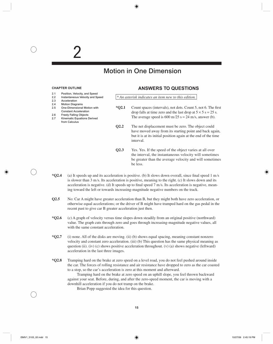
2Motion in One Dimension

CHAPTER OUTLINE

2.1 Position, Velocity, and Speed2.2 Instantaneous Velocity and Speed2.3 Acceleration2.4 Motion Diagrams2.5 One-Dimensional Motion with

Constant Acceleration2.6 Freely Falling Objects2.7 Kinematic Equations Derived

from Calculus

ANSWERS TO QUESTIONS

* An asterisk indicates an item new to this edition.

*Q2.1 Count spaces (intervals), not dots. Count 5, not 6. The fi rst drop falls at time zero and the last drop at 5 × 5 s = 25 s. The average speed is 600 m �25 s = 24 m �s, answer (b).

Q2.2 The net displacement must be zero. The object could have moved away from its starting point and back again, but it is at its initial position again at the end of the time interval.

Q2.3 Yes. Yes. If the speed of the object varies at all over the interval, the instantaneous velocity will sometimes be greater than the average velocity and will sometimes be less.

*Q2.4 (a) It speeds up and its acceleration is positive. (b) It slows down overall, since fi nal speed 1 m �s is slower than 3 m �s. Its acceleration is positive, meaning to the right. (c) It slows down and its acceleration is negative. (d) It speeds up to fi nal speed 7 m �s. Its acceleration is negative, mean-ing toward the left or towards increasing-magnitude negative numbers on the track.

Q2.5 No: Car A might have greater acceleration than B, but they might both have zero acceleration, or otherwise equal accelerations; or the driver of B might have tramped hard on the gas pedal in the recent past to give car B greater acceleration just then.

*Q2.6 (c) A graph of velocity versus time slopes down steadily from an original positive (northward) value. The graph cuts through zero and goes through increasing-magnitude negative values, all with the same constant acceleration.

*Q2.7 (i) none. All of the disks are moving. (ii) (b) shows equal spacing, meaning constant nonzero velocity and constant zero acceleration. (iii) (b) This question has the same physical meaning as question (ii). (iv) (c) shows positive acceleration throughout. (v) (a) shows negative (leftward) acceleration in the last three images.

*Q2.8 Tramping hard on the brake at zero speed on a level road, you do not feel pushed around inside the car. The forces of rolling resistance and air resistance have dropped to zero as the car coasted to a stop, so the car’s acceleration is zero at this moment and afterward.

Tramping hard on the brake at zero speed on an uphill slope, you feel thrown backward against your seat. Before, during, and after the zero-speed moment, the car is moving with a downhill acceleration if you do not tramp on the brake.

Brian Popp suggested the idea for this question.

15

ISMV1_5103_02.indd 15ISMV1_5103_02.indd 15 10/27/06 2:45:19 PM10/27/06 2:45:19 PM

*Q2.9 With original velocity zero, displacement is proportional to the square of time in (1�2)at 2. Making the time one-third as large makes the displacement one-ninth as large, answer (c).

Q2.10 No. Constant acceleration only. Yes. Zero is a constant.

Q2.11 They are the same. After the fi rst ball reaches its apex and falls back downward past the student, it will have a downward velocity of magnitude vi. This velocity is the same as the velocity of the second ball, so after they fall through equal heights their impact speeds will also be the same.

*Q2.12 For the release from rest we have (4 m �s)2 = 02 + 2 gh. For case (i), we have vf2 = (3 m �s)2 + 2 gh =

(3 m �s)2 + (4 m �s)2. Thus answer (d) is true. For case (ii) the same steps give the same answer (d).

*Q2.13 (i) Its speed is zero at b and e. Its speed is equal at a and c, and somewhat larger at d. On the bounce it is moving somewhat slower at f than at d, and slower at g than at c. The assembled answer is d > f > a = c > g > b = e.

(ii) The velocity is positive at a, f, and g, zero at b and e, and negative at c and d, with magnitudes as described in part (i). The assembled answer is f > a > g > b = e > c > d.

(iii) The acceleration has a very large positive value at e. At all the other points it is −9.8 m �s 2. The answer is e > a = b = c = d = f = g.

Q2.14 (b) Above. Your ball has zero initial speed and smaller average speed during the time of fl ight to the passing point. So your ball must travel a smaller distance to the passing point that the ball your friend throws.

16 Chapter 2

SOLUTIONS TO PROBLEMS

Section 2.1 Position, Velocity, and Speed

P2.1 (a) vavg

x

t= = =∆

∆10

5m

2 sm s

(b) vavg = =51 2

m

4 sm s.

(c) vavg

x x

t t= −

−= −

−= −2 1

2 1

5 10

22 5

m m

4 s sm s.

(d) vavg

x x

t t= −

−= − −

−= −2 1

2 1

5 5

43 3

m m

7 s sm s.

(e) vavg

x x

t t= −

−= −

−=2 1

2 1

0 0

8 00 m s

P2.2 (a) vavg = 2 30. m s

(b) v = =m m

s= 16.1 m s

∆∆

x

t

57 5 9 20

3 00

. .

.

−

(c) vavg

x

t= = − =∆

∆57 5 0

11 5.

.m m

5.00 sm s


Motion in One Dimension 17

P2.3 (a) Let d represent the distance between A and B. Let t1 be the time for which the walker has

the higher speed in 5 001

. m s = d

t. Let t2 represent the longer time for the return trip in

− = −3 002

. m sd

t. Then the times are t

d1 5 00

= ( ). m s and t

d2 3 00

= ( ). m s. The average

speed is:

vavg

d d

d= = +

(Total distance

Total time m s/ .5 00 )) + ( ) = ( ) ( )d

d

d

avg

/ . . / .3 00

2

8 00 15 0m s m s m s2 2

v ==( )

=2 15 0

8 003 75

.

..

m s

m sm s

2 2

(b) She starts and fi nishes at the same point A. With total displacement = 0, average

velocity = 0 .

P2.4 x t= 10 2: By substitution, for t

x

s

m

( ) =( ) =

2 0 2 1 3 0

40 44 1 90

. . .

.

(a) vavg

x

t= = =∆

∆50

50 0m

1.0 sm s.

(b) vavg

x

t= = =∆

∆4 1

41 0.

.m

0.1 sm s

Section 2.2 Instantaneous Velocity and Speed

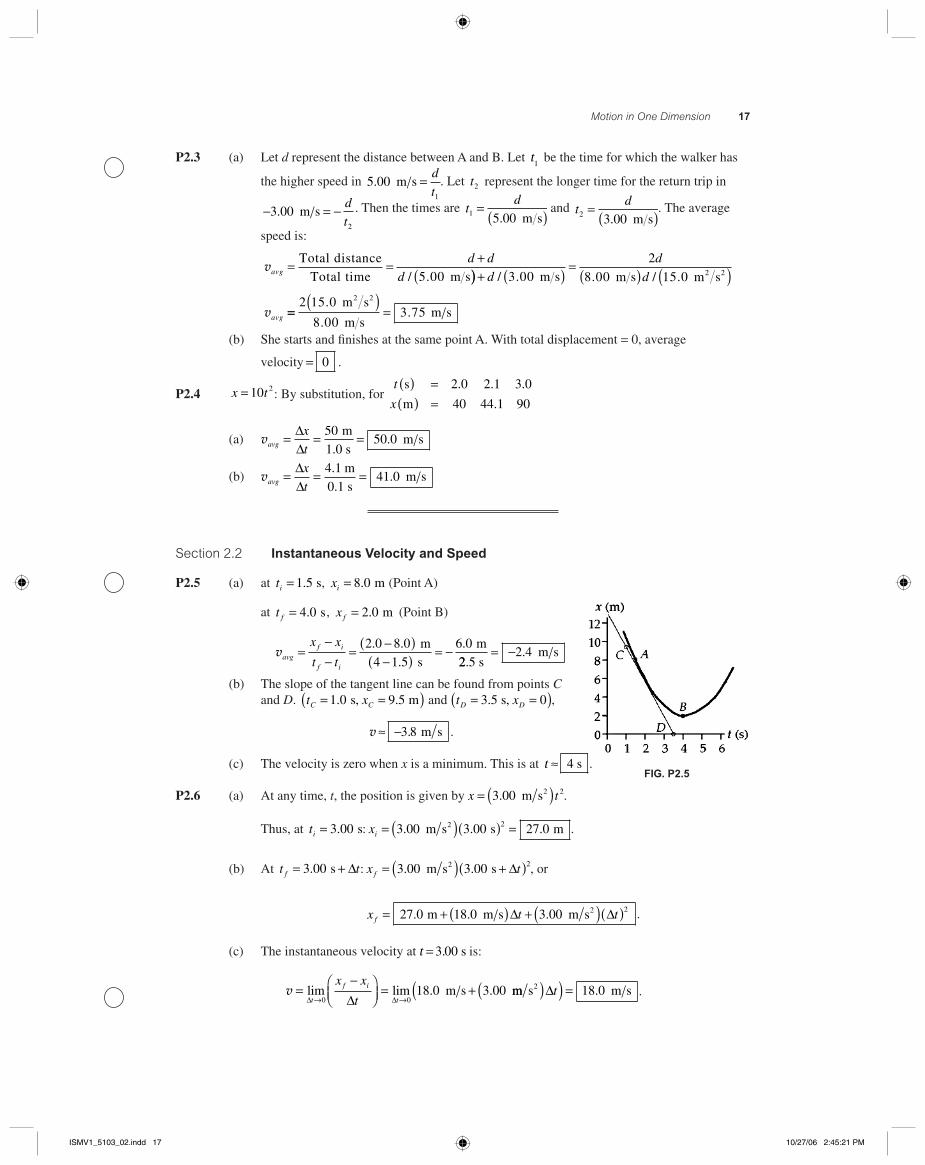
P2.5 (a) at ti = 1 5. s, xi = 8 0. m (Point A)

at t f = 4 0. s, x f = 2 0. m (Point B)

vavgf i

f i

x x

t t=

−−

= −( )−( ) = −2 0 8 0

4 1 5

6 0. .

.

.m

s

m

22.5 sm s= −2 4.

(b) The slope of the tangent line can be found from points C and D. t xC C= =( )1 0 9 5. .s, m and t xD D= =( )3 5 0. s, ,

v ≈ −3 8. m s .

(c) The velocity is zero when x is a minimum. This is at t ≈ 4 s .

P2.6 (a) At any time, t, the position is given by x t= ( )3 00 2. m s2 .

Thus, at ti = 3 00. s: xi = ( )( ) =3 00 3 00 27 02. . .m s s m2 .

(b) At t tf = +3 00. s ∆ : x tf = ( ) +( )3 00 3 00 2. .m s s2 ∆ , or

x t tf = + ( ) + ( )( )27 0 18 0 3 00 2. . .m m s m s2∆ ∆ .

(c) The instantaneous velocity at t = 3 00. s is:

v =−⎛

⎝⎜⎞⎠⎟

= +→ →

lim lim . .∆ ∆∆t

f i

t

x x

t0 018 0 3 00m s mm s m s2( )( ) =∆t 18 0. .

FIG. P2.5


18 Chapter 2

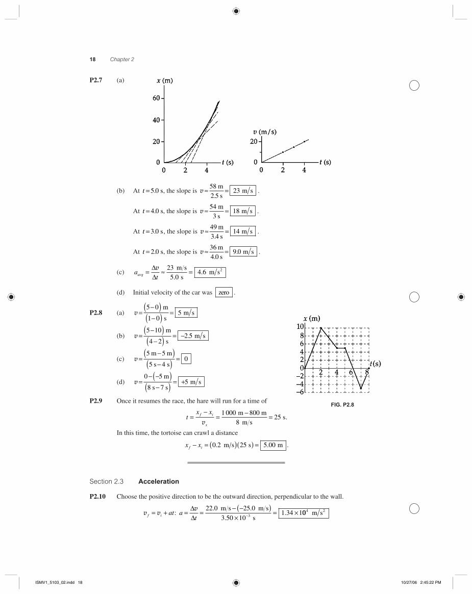
P2.7 (a)

(b) At t = 5 0. s, the slope is v ≈ =5823

m

2.5 sm s .

At t = 4 0. s, the slope is v ≈ =541

m

3 s8 m s .


9 m

3.4 s4 m s .


6 m

4.0 s.0 m s .

(c) atavg = ≈ =∆

∆v 23

5 04 6

m s

sm s2

..

(d) Initial velocity of the car was zero .

P2.8 (a) v =−( )−( ) =

5 0

1 05

m

sm s

(b) v =−( )−( ) = −

5 10

4 22 5

m

sm s.

(c) v =−( )−( ) =

5 5

5 40

m m

s s

(d) v =− −( )

−( ) = +0 5

8 75

m

s sm s

P2.9 Once it resumes the race, the hare will run for a time of

tx xf i

x

=−

= − =v

1 00025

m 800 m

8 m ss.

In this time, the tortoise can crawl a distance

x xf i− = ( )( ) =0 2 25 5 00. .m s s m .

Section 2.3 Acceleration

P2.10 Choose the positive direction to be the outward direction, perpendicular to the wall.

v vf i at= + : at

= =− −( )×

= ×−

∆∆v 22 0 25 0

3 50 101 34 13

. .

..

m s m s

s004 m s2

FIG. P2.8



P2.11 (a) Acceleration is constant over the fi rst ten seconds, so at the end of this interval

v vf i at= + = + ( )( ) =0 2 00 10 0 20 0. . .m s s m s2 .

Then a = 0 so v is constant from t =10 0. s to t =15 0. s. And over the last fi ve seconds the velocity changes to

v vf i at= + = + −( )( ) =20 0 3 00 5 00 5 00. . . .m s m s s m2 ss .

(b) In the fi rst ten seconds,

x x t atf i i= + + = + + ( )( ) =v1

20 0

1

22 00 10 0 12 2. .m s s2 000 m.

Over the next fi ve seconds the position changes to

x x t atf i i= + + = + ( )( ) + =v1

2100 20 0 5 00 0 22 m m s s. . 000 m.

And at t = 20 0. s,

x x t atf i i= + + = + ( )( ) + −v1

2200 20 0 5 00

1

22 m m s s. . 33 00 5 00 2622. .m s s m2( )( ) = .

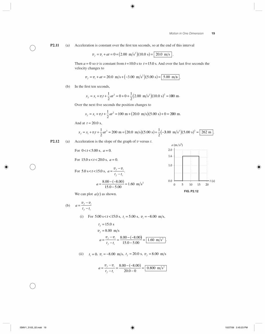
P2.12 (a) Acceleration is the slope of the graph of v versus t.

For 0 5 00< <t . s, a = 0.

For 15 0 20 0. .s s< <t , a = 0.

For 5 0 15 0. .s s< <t , at t

f i

f i

=−−

v v.

a = − −( )−

=8 00 8 00

15 0 5 001 60

. .

. .. m s2

We can plot a t( ) as shown.

(b) at t

f i

f i

=−−

v v

(i) For 5 00 15 0. .s s< <t , ti = 5 00. s, vi = −8 00. m s,

t

at t

f

f

f i

f i

=

=

=−−

= − −(

15 0

8 00

8 00 8 00

.

.

. .

s

m sv

v v ))−

=15 0 5 00

1 60. .

. .m s2

(ii) ti = 0, vi = −8 00. m s, t f = 20 0. s, v f = 8 00. m s

at t

f i

f i

=−−

= − −( )−

=v v 8 00 8 00

20 0 00 800

. .

.. m s2

FIG. P2.12

0.0

1.0

1050 15t (s)

20

1.6

2.0

a (m/s2)


20 Chapter 2

P2.13 x t t= + −2 00 3 00 2. . , so v = = −dx

dtt3 00 2 00. . , and a

d

dt= = −v

2 00.

At t = 3 00. s:

(a) x = + −( ) =2 00 9 00 9 00 2 00. . . .m m

(b) v = −( ) = −3 00 6 00 3 00. . .m s m s

(c) a = −2 00. m s2

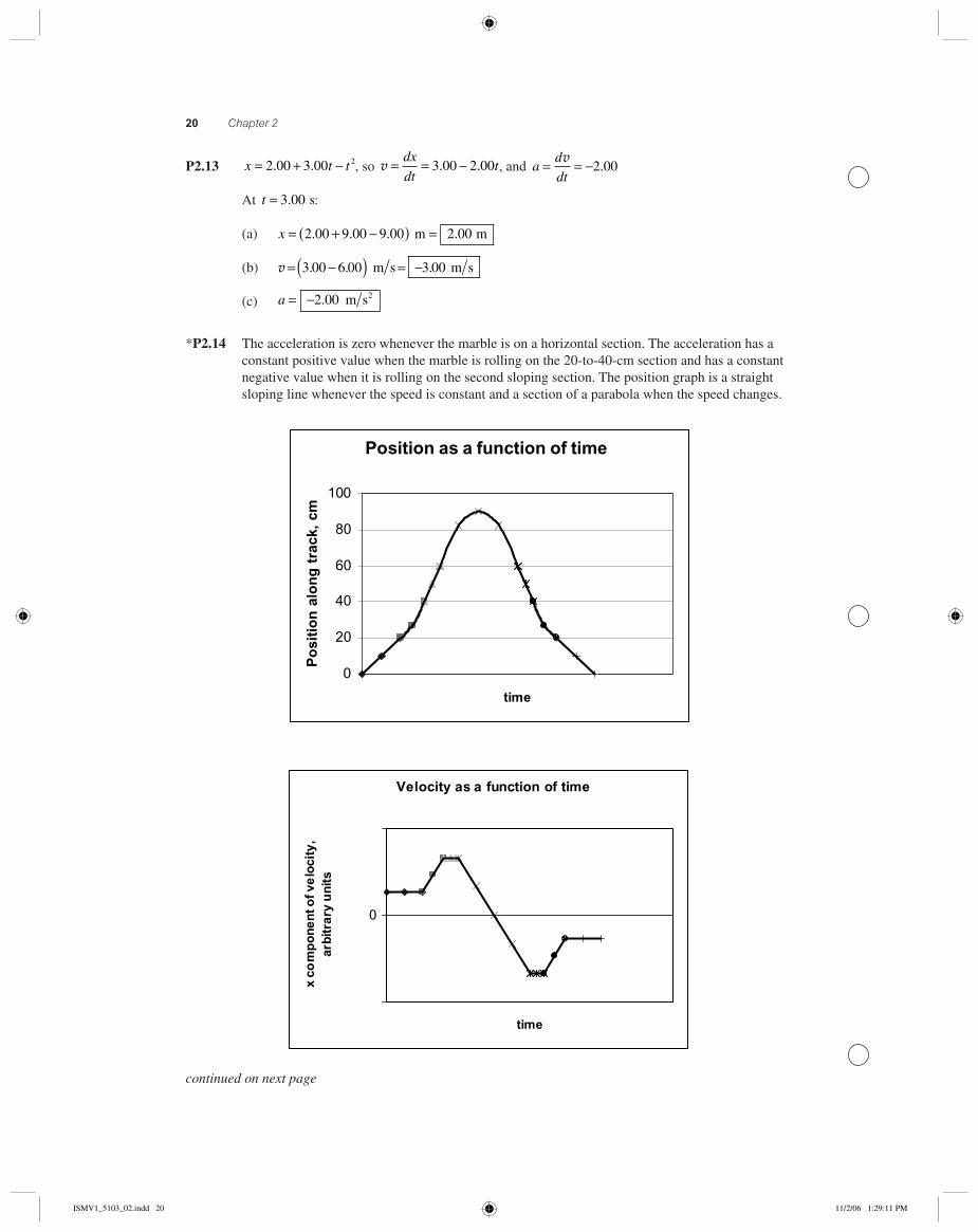
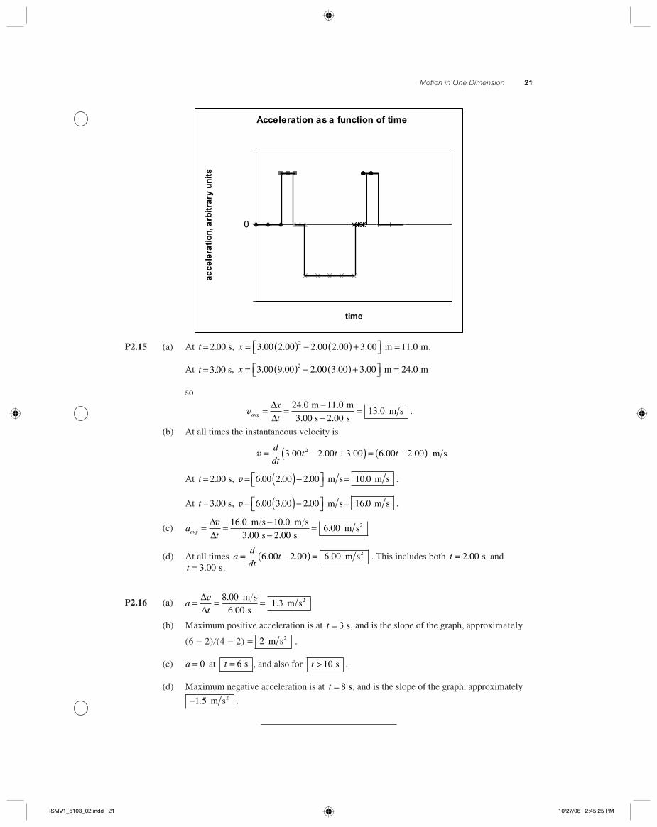
*P2.14 The acceleration is zero whenever the marble is on a horizontal section. The acceleration has a constant positive value when the marble is rolling on the 20-to-40-cm section and has a constant negative value when it is rolling on the second sloping section. The position graph is a straight sloping line whenever the speed is constant and a section of a parabola when the speed changes.

Position as a function of time

0

20

40

60

80

100

time

Po

siti

on

alo

ng

tra

ck,

cm

continued on next page

Velocity as a function of time

0

time

x co

mp

on

en

t of v

elo

city

,ar

bit

rary

un

its



Acceleration as a function of time

�

time

acce

lera

tio

n, a

rbit

rary

un

its

P2.15 (a) At t = 2 00. s, x = ( ) − ( ) +⎡⎣ ⎤⎦ =3 00 2 00 2 00 2 00 3 00 11 02. . . . . .m m.

At t = 3 00. s, x = ( ) − ( ) +⎡⎣ ⎤⎦ =3 00 9 00 2 00 3 00 3 00 24 02. . . . . .m m

so

vavg

x

t= = −

−=∆

∆24 0 11 0

2 0013 0

. .

..

m m

3.00 s sm ss .

(b) At all times the instantaneous velocity is

v = − +( ) = −( )d

dtt t t3 00 2 00 3 00 6 00 2 002. . . . . m s

At t = 2 00. s, v = ( )−⎡⎣ ⎤⎦ =6 00 2 00 2 00 10 0. . . .m s m s .

At t = 3 00. s, v = ( )−⎡⎣ ⎤⎦ =6 00 3 00 2 00 16 0. . . .m s m s .

(c) atavg = = −

−=∆

∆v 16 0 10 0

3 00 2 006 00

. .

. ..

m s m s

s sm s2

(d) At all times ad

dtt= −( ) =6 00 2 00 6 00. . . m s2 . This includes both t = 2 00. s and

t = 3 00. s.

P2.16 (a) at

= = =∆∆

v 8 00

6 001 3

.

..

m s

sm s2

(b) Maximum positive acceleration is at t = 3 s, and is the slope of the graph, approximately

(6 − 2)�(4 − 2) = 2 m s2 .

(c) a = 0 at t = 6 s , and also for t > 10 s .

(d) Maximum negative acceleration is at t = 8 s, and is the slope of the graph, approximately

−1 5. m s2 .


22 Chapter 2

Section 2.4 Motion Diagrams

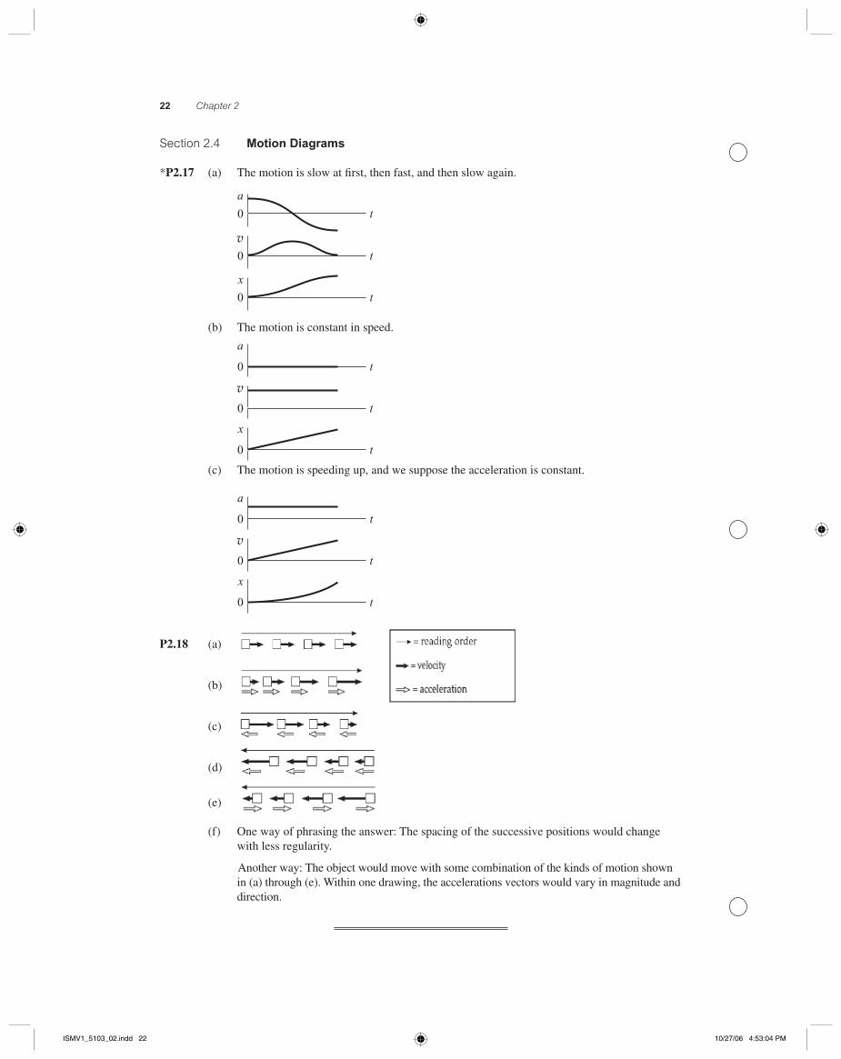
*P2.17 (a) The motion is slow at fi rst, then fast, and then slow again.

t

t

t0

a

0

0

x

(b) The motion is constant in speed.

t0

x

t0

t0

a

(c) The motion is speeding up, and we suppose the acceleration is constant.

t0

x

t0

t0

a

P2.18 (a)

(b)

(c)

(d)

(e)

(f ) One way of phrasing the answer: The spacing of the successive positions would change with less regularity.

Another way: The object would move with some combination of the kinds of motion shown in (a) through (e). Within one drawing, the accelerations vectors would vary in magnitude and direction.



Section 2.5 One-Dimensional Motion with Constant Acceleration

*P2.19 (a) vf = v

i + at = 13 m �s − 4 m �s2 (1 s) = 9.00 m �s

(b) vf = v

i + at = 13 m �s − 4 m �s2 (2 s) = 5.00 m �s

(c) vf = v

i + at = 13 m �s − 4 m �s2 (2.5 s) = 3.00 m �s

(d) vf = v

i + at = 13 m �s − 4 m �s2 (4 s) = −3.00 m �s

(e) vf = v

i + at = 13 m �s − 4 m �s2 (−1 s) = 17.0 m �s

(f ) The graph of velocity versus time is a slanting straight line, having the value 13 m �s at 10:05:00 a.m. on the certain date, and sloping down by 4 m �s for every second thereafter.

(g) If we also know the velocity at any one instant, then knowing the value of the constant acceleration tells us the velocity at all other instants.

P2.20 (a) x x tf i i f− = +( )1

2v v becomes 40

1

22 80 8 50m m s s= +( )( )vi . . which yields

vi = 6 61. m s .

(b) at

f i=−

= − = −v v 2 80 6 61

8 500 448

. .

..

m s m s

sm s2

P2.21 Given vi = 12 0. cm s when x ti = =( )3 00 0. cm , and at t = 2 00. s, x f = −5 00. cm,

x x t atf i i− = +v1

22 : − − = ( ) + ( )5 00 3 00 12 0 2 00

1

22 00 2. . . . .a

− = +8 00 24 0 2. . a a = − = −32 0

216 0

.. cm s2 .

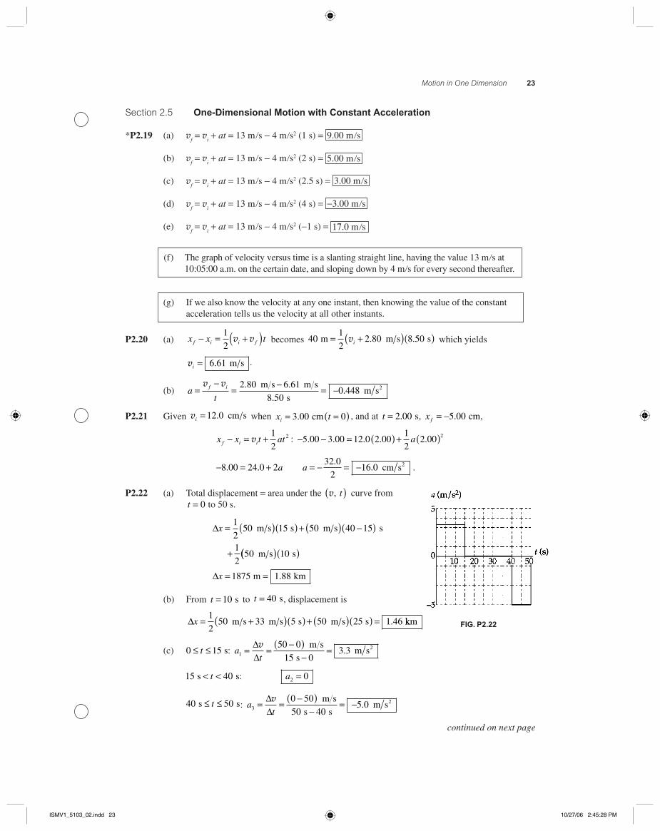
P2.22 (a) Total displacement = area under the v, t( ) curve fromt = 0 to 50 s.

∆x = ( )( ) + ( ) −( )

+

1

250 15 50 40 15

1

250

m s s m s s

m s(( )( )

= =

10

1875 1 88

s

m km∆x .

(b) From t = 10 s to t = 40 s, displacement is

∆x = +( )( ) + ( )( ) =1

250 33 5 50 25 1 46m s m s s m s s . kkm

(c) 0 15≤ ≤t s: at1

50 0

15 03 3= = −( )

−=∆

∆v m s

sm s2.

15 40s s< <t : a2 0=

40 50s s≤ ≤t : at3

0 50

50 405 0= = −( )

−= −∆

∆v m s

s sm s2.

FIG. P2.22



24 Chapter 2

(d) (i) x a t t1 12 20

1

2

1

23 3= + = ( ). m s2 or x t1

21 67= ( ). m s2

(ii) x t2

1

215 50 0 50 15= ( ) −[ ]+ ( ) −( )s m s m s s or x t2 50 375= ( ) −m s m

(iii) For 40 50s s≤ ≤t ,

xt

t3 0=

=⎛⎝⎜

⎞⎠⎟

+area under vs

from to 40 s

v 11

240 50 403

2a t t−( ) + ( ) −( )s m s s

or

x t32375 1 250

1

25 0 40 50= + + −( ) −( ) +m m m s s m s2. (( ) −( )t 40 s

which reduces to

x t t32250 2 5 4 375= ( ) − ( ) −m s m s m2. .

(e) v = =total displacement

total elapsed time

1875 m

sm s

5037 5= .

P2.23 (a) vi = 100 m s, a = −5 00. m s2, v vf i at= + so 0 100 5= − t , v vf i f ia x x2 2 2= + −( ) so

0 100 2 5 00 02= ( ) − ( ) −( ). x f . Thus x f = 1 000 m and t = 20 0. s .

(b) 1 000 m is greater than 800 m. With this acceleration

the plane would overshoot the runway: it cannot land .

*P2.24 (a) For the fi rst car the speed as a function of time is v = vi + at = − 3.5 cm �s + 2.4 cm �s2 t .

For the second car, the speed is + 5.5 cm�s + 0. Setting the two expressions equal gives

−3.5 cm�s + 2.4 cm �s2 t = 5.5 cm�s so t = (9 cm�s) �(2.4 cm �s2) = 3.75 s .

(b) The fi rst car then has speed −3.5 cm�s + (2.4 cm�s2)(3.75 s) = 5.50 cm �s , and this is the constant speed of the second car also.

(c) For the fi rst car the position as a function of time is xi + v

it + (1�2)at2 = 15 cm −

(3.5 cm�s)t + (0.5)(2.4 cm�s2) t2.

For the second car, the position is 10 cm + (5.5 cm �s)t + 0.

At passing, the positions are equal: 15 cm − (3.5 cm �s)t + (1.2 cm �s2) t 2 = 10 cm + (5.5 cm �s)t (1.2 cm �s2) t2 − (9 cm �s) t + 5 cm = 0.

We solve with the quadratic formula:

t = ± − = + − =9 9 4 1 2 5

2 1 2

9 57

2 4

9 57

2 4

2 ( . )( )

( . ) . .and 66 90. s and 0.604 s

(d) At 0.604 s, the second and also the fi rst car’s position is 10 cm + (5.5 cm �s)0.604 s = 13.3 cm .

At 6.90 s, both are at position 10 cm + (5.5 cm �s)6.90 s = 47.9 cm .


ISMV1_5103_02.indd 24ISMV1_5103_02.indd 24 11/2/06 11:12:23 AM11/2/06 11:12:23 AM


(e) The cars are initially moving toward each other, so they soon share the same position x when their speeds are quite different, giving one answer to (c) that is not an answer to (a). The fi rst car slows down in its motion to the left, turns around, and starts to move toward the right, slowly at fi rst and gaining speed steadily. At a particular moment its speed will be equal to the constant rightward speed of the second car. The distance between them will at that moment be staying constant at its maximum value. The dis-tance between the cars will be far from zero, as the accelerating car will be far to the left of the steadily moving car. Thus the answer to (a) is not an answer to (c). Eventually the accelerating car will catch up to the steadily-coasting car, whizzing past at higher speed than it has ever had before, and giving another answer to (c) that is not an answer to (a). A graph of x versus t for the two cars shows a parabola originally sloping down and then curving upward, intersecting twice with an upward-sloping straight line. The parabola and straight line are running parallel, with equal slopes, at just one point in between their intersections.

P2.25 In the simultaneous equations:

v v

v v

xf xi x

f i xi xf

a t

x x t

= +

− = +( )⎧⎨⎪

⎩⎪

⎫⎬⎪

⎭⎪1

2

we have v v

v v

xf xi

xi xf

= − ( )( )

= +(5 60 4 20

62 41

2

. .

.

m s s

m

2

))( )

⎧⎨⎪

⎩⎪

⎫⎬⎪

⎭⎪4 20. s

.

So substituting for vxi gives 62 41

25 60 4 20 4 20. . . .m m s s2= + ( )( ) +⎡⎣ ⎤⎦v vxf xf s( )

14 91

25 60 4 20. . .m s m s s2= + ( )( )vxf

.

Thus

vxf = 3 10. m s .

P2.26 Take any two of the standard four equations, such as

v v

v v

xf xi x

f i xi xf

a t

x x t

= +

− = +( )⎧⎨⎪

⎩⎪

⎫⎬⎪

⎭⎪1

2

.

Solve one for vxi , and substitute into the other: v vxi xf xa t= −

x x a t tf i xf x xf− = − +( )1

2v v .

Thus

x x t a tf i xf x− = −v1

22 .

We note that the equation is dimensionally correct. The units are units of length in each term.

Like the standard equation x x t a tf i xi x− = +v1

22, this equation represents that displacement

is a quadratic function of time. Our newly derived equation gives us for the situation back in problem 25,

62 4 4 201

25 60 4 20 2. . . .m s m s s2= ( ) − −( )( )vxf

vxf = − =62 4 49 43 10

. ..

m m

4.20 sm s .


26 Chapter 2

P2.27 (a) at

f i=−

= ( )= − = −

v v 632 5280 3600

1 40662 202

/

.ft s2 mm s2

(b) x t atf i= + = ( )⎛⎝⎜

⎞⎠⎟

( ) −v1

2632

5 280

3 6001 40

1

2662 . 22 1 40 649 1982( )( ) = =. ft m

P2.28 (a) Compare the position equation x t t= + −2 00 3 00 4 00 2. . . to the general form

x x t atf i i= + +v1

22

to recognize that xi = 2 00. m, vi = 3 00. m s, and a = −8 00. m s2. The velocity equation, v v

f iat= + , is then

v f t= − ( )3 00 8 00. .m s m s2 .

The particle changes direction when v f = 0, which occurs at t = 3

8s. The position at this time is

x = + ( )⎛⎝

⎞⎠ − ( )⎛

⎝2 00 3 003

84 00

3

8. . .m m s s m s s2 ⎞⎞

⎠ =2

2 56. m .

(b) From x x t atf i i= + +v1

22, observe that when x xf i= , the time is given by t

ai= −

2v. Thus,

when the particle returns to its initial position, the time is

t =− ( )−

=2 3 00

8 00

3

4

.

.

m s

m ss2

and the velocity is v f = − ( )⎛⎝

⎞⎠ = −3 00 8 00

3

43 00. . .m s m s s m s2 .

P2.29 We have vi = ×2 00 104. m s, v f = ×6 00 106. m s, x xf i− = × −1 50 10 2. m.

(a) x x tf i i f− = +( )1

2v v : t

x xf i

i f

=−( )

+=

×( )× +

−2 2 1 50 10

2 00 10 6

2

4v v

.

.

m

m s ...

00 104 98 106

9

×= × −

m ss

(b) v vf i x f ia x x2 2 2= + −( ) :

ax xxf i

f i

=−−

=×( ) − ×v v2 2 6 2 4

2

6 00 10 2 00 10

( )

. .m s mm s

mm s2( )

×= ×−

2

215

2 1 50 101 20 10

( . ).

P2.30 (a) Along the time axis of the graph shown, let i = 0 and f tm= . Then v vxf xi xa t= + gives vc m ma t= +0

atm

c

m

= v.

(b) The displacement between 0 and tm is

x x t a tt

t tf i xi xc

mm c m− = + = + =v

vv

1

20

1

2

1

22 2 .

The displacement between tm and t0 is

x x t a t t tf i xi x c m− = + = −( ) +v v1

202

0 .

The total displacement is

∆x t t t t tc m c c m c m= + − = −⎛⎝

⎞⎠

1

2

1

20 0v v v v .




(c) For constant vc and t0 , ∆x is minimized by maximizing tm to t tm = 0. Then

∆x t tt

cc

min = −⎛⎝

⎞⎠ =v

v0 0

01

2 2.

(e) This is realized by having the servo motor on all the time.

(d) We maximize ∆x by letting tm approach zero. In the limit ∆x t tc c= −( ) =v v0 00 .

(e) This cannot be attained because the acceleration must be fi nite.

P2.31 Let the glider enter the photogate with velocity vi and move with constant acceleration a. For its motion from entry to exit,

x x t a t

t a t t

f i xi x

i d d d d

d

= + +

= + + =

=

v

v v

v

1

2

01

2

2

2� ∆ ∆ ∆

vvi da t+ 1

2∆

(a) The speed halfway through the photogate in space is given by

v v v vhs i i d da a t2 2 222

= + ⎛⎝⎜

⎞⎠⎟ = +� ∆ .

v v vhs i d da t= +2 ∆ and this is not equal to vd unless a = 0 .

(b) The speed halfway through the photogate in time is given by v vht i

dat

= +⎛

⎝⎜⎞

⎠⎟∆2

and this is

equal to vd as determined above.

P2.32 Take the original point to be when Sue notices the van. Choose the origin of the x-axis at Sue’s car. For her we have xis = 0, vis = 30 0. m s, as = −2 00. m s2 so her position is given by

x t x t a t ts is is s( ) = + + = ( ) + −v1

230 0

1

22 002 . .m s m s22( )t 2.

For the van, xiv = 155 m, v vi = 5 00. m s, av = 0 and

x t x t a t ti iv v v vv( ) = + + = + ( ) +1

2155 5 00 02 . m s .

To test for a collision, we look for an instant tc when both are at the same place:

30 0 155 5 00

0 25 0 155

2

2

. .

. .

t t t

t t

c c c

c c

− = +

= − +

From the quadratic formula

tc =± ( ) − ( )

=25 0 25 0 4 155

213 6

2. .. s or 11 4. s .

The roots are real, not imaginary, so there is a collision . The smaller value is the collision time. (The larger value tells when the van would pull ahead again if the vehicles could move through each other). The wreck happens at position

155 5 00 11 4 212m m s s m+ ( )( ) =. . .


28 Chapter 2

*P2.33 (a) Starting from rest and accelerating at ab = ⋅13 0. mi h s, the bicycle reaches its maximum speed of vb,max .= 20 0 mi h in a time

tab

b

b,

,max .

..1

0 20 0

13 01 54=

−=

⋅=

v mi h

mi h ss .

Since the acceleration ac of the car is less than that of the bicycle, the car cannot catch the bicycle until some time t tb> ,1 (that is, until the bicycle is at its maximum speed and coast-ing). The total displacement of the bicycle at time t is

∆x a t t tb b b b b= + −( )

=⎛

1

2

1 47

1

12

1, ,max ,

.

v

ft s

mi h⎝⎝⎜⎞⎠⎟

⎛⎝

⎞⎠ ( ) + ( ) −1

213 0 1 54 20 02. . .

mi h

ss mi h t 11 54

29 4 22 6

.

. .

s

ft s ft

( )⎡⎣⎢

⎤⎦⎥

= ( ) −t

The total displacement of the car at this time is

∆x a tc c= =⎛⎝⎜

⎞⎠⎟

⎛⎝

1

2

1 47

1

1

29 002 ..

ft s

mi h

mi h

s⎞⎞⎠

⎡⎣⎢

⎤⎦⎥

= ( )t t2 26 62. ft s

At the time the car catches the bicycle ∆ ∆x xc b= . This gives

6 62 29 4 22 62. . .ft s ft s ft2( ) = ( ) −t t or t t2 24 44 3 42 0− ( ) + =. .s s

that has only one physically meaningful solution t tb> ,1. This solution gives the total time

the bicycle leads the car and is t = 3 45. s .

(b) The lead the bicycle has over the car continues to increase as long as the bicycle is moving faster than the car. This means until the car attains a speed of v vc b= =,max .20 0 mi h. Thus, the elapsed time when the bicycle’s lead ceases to increase is

tab

c

= =⋅

=v ,max .

..

20 0

9 002 22

mi h

mi h ss

At this time, the lead is

∆ ∆ ∆ ∆x x x xb c b c t−( ) = −( ) = ( )

=max .. .

2 2229 4 2

sft s 222 22 6 6 62 2 22 2s ft ft s s2( ) −⎡⎣ ⎤⎦ − ( )( )⎡⎣ ⎤. . . ⎦⎦

or ∆ ∆x xb c−( ) =max

.10 0 ft .

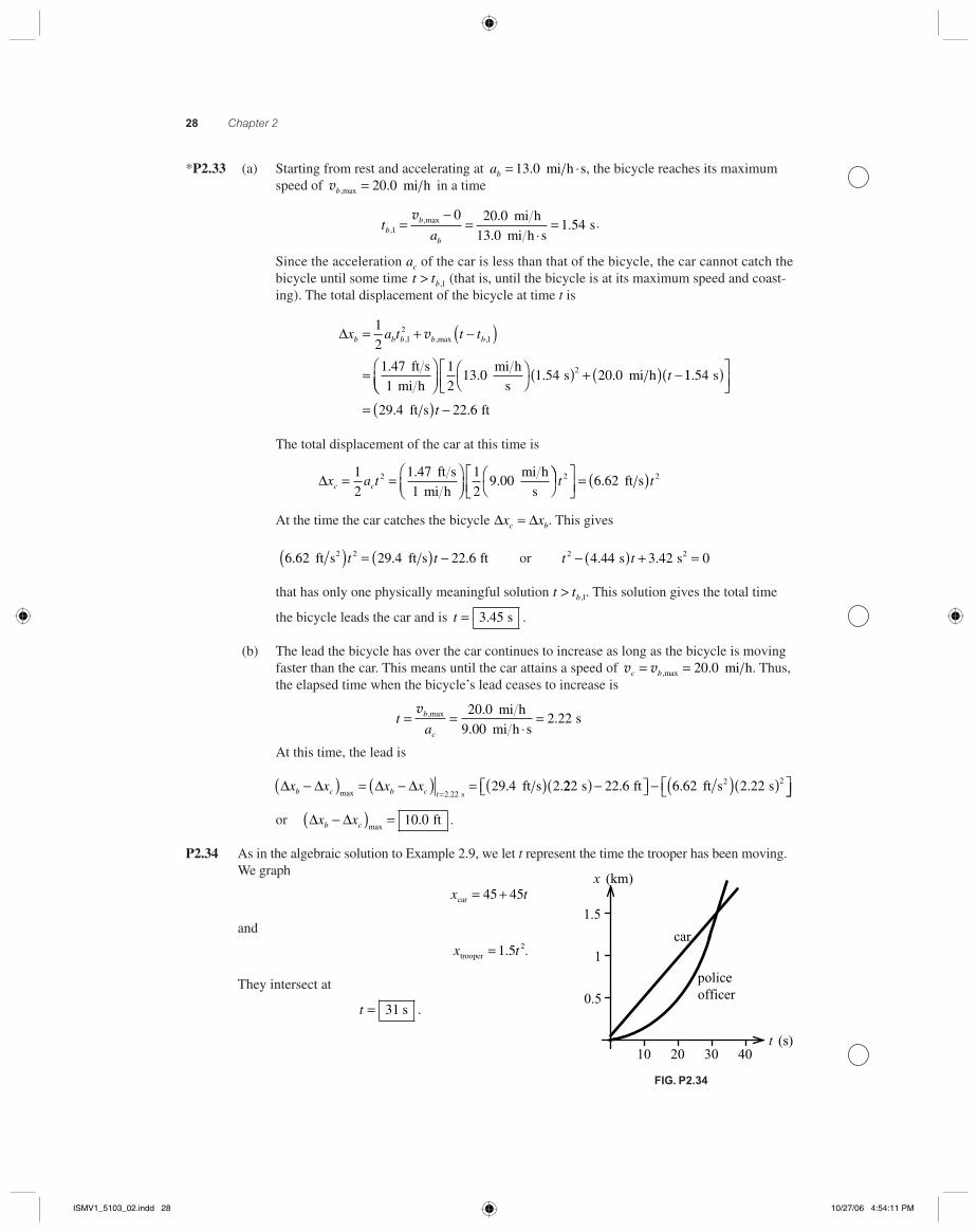
P2.34 As in the algebraic solution to Example 2.9, we let t represent the time the trooper has been moving. We graph

x tcar = +45 45

and

x ttrooper = 1 5 2. .

They intersect at

t = 31 s .

FIG. P2.34

x (km)

t (s)10 20 30 40

0.5

1

1.5

car

policeofficer



*P2.35 (a) Let a stopwatch start from t = 0 as the front end of the glider passes point A. The average speed of the glider over the interval between t = 0 and t = 0.628 s is 12.4 cm�(0.628 s) = 19.7 cm �s , and this is the instantaneous speed halfway through the time interval, at

t = 0.314 s.

(b) The average speed of the glider over the time interval between 0.628 + 1.39 = 2.02 s and 0.628 + 1.39 + 0.431 = 2.45 s is 12.4 cm �(0.431 s) = 28.8 cm �s and this is the instantaneous speed at the instant t = (2.02 + 2.45) �2 = 2.23 s.

Now we know the velocities at two instants, so the acceleration is found from [(28.8 − 19.7) cm �s] � [(2.23 − 0.314) s] = 9.03 �1.92 cm �s2 = 4.70 cm �s2 .

(c) The time required to pass between A and B is suffi cient to fi nd the acceleration, more directly than we could fi nd it from the distance between the points.

Section 2.6 Freely Falling Objects

*P2.36 Choose the origin y t= =( )0 0, at the starting point of the cat and take upward as positive.

Then yi = 0, vi = 0, and a g= − = −9 80. m s2. The position and the velocity at time t become:

y y t atf i i− = +v1

22 : y gt tf = − = − ( )1

2

1

29 802 2. m s2

and

v vf i at= + : v f gt t= − = −( )9 80. m s2 .

(a) at t = 0 1. s: yf = − ( )( ) = −1

29 80 0 0 049 02. .m s .1 s m2

at t = 0 2. s: yf = − ( )( ) = −1

29 80 0 0 1962. .m s .2 s m2

at t = 0 3. s: yf = − ( )( ) = −1

29 80 0 0 4412. .m s .3 s m2

(b) at t = 0 1. s: v f = −( )( ) = −9 80 0 0 980. .m s .1 s m s2

at t = 0 2. s: v f = −( )( ) = −9 80 0 1 96. .m s .2 s m s2

at t = 0 3. s: v f = −( )( ) = −9 80 0 2 94. .m s .3 s m s2


30 Chapter 2

P2.37 Assume that air resistance may be neglected. Then, the acceleration at all times during the fl ight is that due to gravity, a g= − = −9 80. m s2. During the fl ight, Goff went 1 mile (1 609 m) up and then 1 mile back down. Determine his speed just after launch by considering his upward fl ight:

v v vf i f i ia y y2 2 22 0 2 9 80 1 609= + −( ) = − ( )( ): . m s m2

vvi = 178 m s.

His time in the air may be found by considering his motion from just after launch to just before impact:

y y t atf i i− = +v1

22: 0 178

1

29 80 2= ( ) − −( )m s m s2t t. .

The root t = 0 describes launch; the other root, t = 36 2. s, describes his fl ight time. His rate of pay is then

pay rate = = ( )( ) =$ .

.. $ .

1 00

36 20 027 6 3 600 99 3

s$ s s h h .

We have assumed that the workman’s fl ight time, “a mile,” and “a dollar,” were measured to three-digit precision. We have interpreted “up in the sky” as referring to the free fall time, not to the launch and landing times.

Both the takeoff and landing times must be several seconds away from the job, in order for Goff to survive to resume work.

P2.38 We have y gt t yf i i

= − + +1

22 v

0 4 90 8 00 30 02= −( ) − ( ) +. . .m s m s m2 t t .

Solving for t,

t = ± +−

8 00 64 0 588

9 80

. .

..

Using only the positive value for t, we fi nd that t = 1 79. s .

P2.39 (a) y y t atf i i− = +v1

22 : 4 00 1 50 4 90 1 50 2. . . .= ( ) − ( )( )vi and vi = 10 0. m s upward .

(b) v vf i at= + = − ( )( ) = −10 0 9 80 1 50 4 68. . . . m s

v f = 4 68. m s downward

P2.40 The bill starts from rest vi = 0 and falls with a downward acceleration of 9 80. m s2 (due to gravity). Thus, in 0.20 s it will fall a distance of

∆y t gti= − = − ( )( ) = −v1

20 4 90 0 20 0 202 2. . .m s s m2 .

This distance is about twice the distance between the center of the bill and its top edge ≈( )8 cm . Thus, David will be unsuccessful.



P2.41 (a) v vf i gt= − : v f = 0 when t = 3 00. s, and g = 9 80. m s2. Therefore,

vi gt= = ( )( ) =9 80 3 00 29 4. . .m s s m s2 .

(b) y y tf i f i− = +( )1

2v v

y yf i− = ( )( ) =1

229 4 3 00 44 1. . . m s s m

*P2.42 We can solve (a) and (b) at the same time by assuming the rock passes the top of the wall and fi nding its speed there. If the speed comes out imaginary, the rock will not reach this elevation.

vf2 = v

i2 + 2a(x

f − x

i) = (7.4 m�s)2 − 2(9.8 m�s2)(3.65 m − 1.55 m) = 13.6 m2�s2

so the rock does reach the top of the wall with vf = 3.69 m�s .

(c) We fi nd the fi nal speed, just before impact, of the rock thrown down:

vf2 = v

i2 + 2a(x

f − x

i) = (−7.4 m �s)2 − 2(9.8 m �s2)(1.55 m − 3.65 m) = 95.9 m2 �s2

vf = −9.79 m �s. The change in speed of the rock thrown down is � 9.79 − 7.4 � = 2.39 m �s

(d) The magnitude of the speed change of the rock thrown up is � 7.4 − 3.69 � = 3.71 m�s.

This does not agree with 2.39 m �s.

The upward-moving rock spends more time in fl ight, so the planet has more time to change its speed.

P2.43 Time to fall 3.00 m is found from the equation describing position as a function of time, with

vi = 0, thus: 3 001

29 80 2. . m m s2= ( )t , giving t = 0 782. s.

(a) With the horse galloping at 10 0. m s, the horizontal distance is vt = 7 82. m .

(b) from above t = 0 782. s

P2.44 y t= 3 00 3. : At t = 2 00. s, y = ( ) =3 00 2 00 24 03

. . . m and

vy

dy

dtt= = = ↑9 00 36 02. . m s .

If the helicopter releases a small mailbag at this time, the mailbag starts its free fall with velocity 36 m�s upward. The equation of motion of the mailbag is

y y t gt t tb bi i= + − = + − ( )v1

224 0 36 0

1

29 802 2. . . .

Setting yb = 0,

0 24 0 36 0 4 90 2= + −. . .t t .

Solving for t, (only positive values of t count), t = 7 96. s .


32 Chapter 2

P2.45 We assume the object starts from rest. Consider the last 30 m of its fall. We fi nd its speed 30 m above the ground:

y y t a tf i yi y

yi

= + +

= + ( ) + −

v

v

1

2

0 30 1 51

29 8

2

m s m. . ss s

m m

1.5 sm s

2( )( )

= − + = −

1 5

30 11 012 6

2.

..vyi ..

Now consider the portion of its fall above the 30 m point:

v vyf yi y f ia y y2 2

2

2

12 6 0 2 9 8

= + −( )−( ) = + −. .m s m s2(( )

=−

= −

∆

∆

y

y160

19 68 16

m s

m sm

2 2

2.. .

Its original height was then 30 8 16 38 2 m m m+ − =. . .

Section 2.7 Kinematic Equations Derived from Calculus

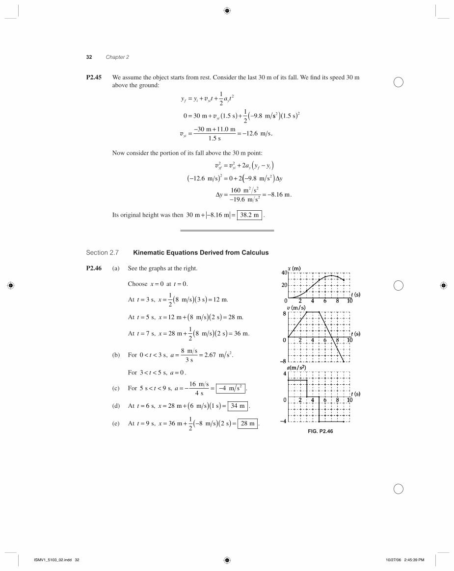
P2.46 (a) See the graphs at the right.

Choose x = 0 at t = 0.

At t = 3 s, x = ( )( ) =1

28 3 12 m s s m.

At t = 5 s, x = + ( )( ) =12 8 2 28 m m s s m.

At t = 7 s, x = + ( )( ) =281

28 2 36 m m s s m.

(b) For 0 3< <t s, a = =8

32 67

m s

s m s2. .

For 3 5< <t s, a = 0 .

(c) For 5 9 s s< <t , a = − = −16

44

m s

s m s2 .

(d) At t = 6 s, x = + ( )( ) =28 6 1 34 m m s s m .

(e) At t = 9 s, x = + −( )( ) =361

28 2 28 m m s s m .

FIG. P2.46



P2.47 (a) Jda

dt= = constant

da Jdt=

a J dt Jt c= = +∫ 1

but a ai= when t = 0 so c ai1 = . Therefore, a Jt ai= +

ad

dtd adt

adt Jt a dt Jt a t ci i

=

=

= = +( ) = + +∫ ∫

v

v

v1

22

2

but v v= i when t = 0, so c i2 = v and v v= + +1

22Jt a ti i

v

v

v v

=

=

= = + +⎛⎝

⎞⎠

=

∫ ∫

dx

dtdx dt

x dt Jt a t dt

x J

i i

1

2

1

6

2

tt a t t c

x x

i i

i

3 23

1

2+ + +

=

v

when t = 0, so c xi3 = . Therefore, x Jt a t t xi i i= + + +1

6

1

23 2 v .

(b)

a Jt a J t a Ja ti i i2 2 2 2 2 2= +( ) = + +

a a J t Ja ti i

2 2 2 2 2= + +( )

a a J Jt a ti i2 2 22

1

2= + +⎛

⎝⎜⎞⎠⎟

Recall the expression for v: v v= + +1

22Jt a ti i . So v v−( ) = +i iJt a t

1

22 . Therefore,

a a Ji i2 2 2= + −( )v v .


34 Chapter 2

P2.48 (a) ad

dt

d

dtt t= = − × + ×⎡⎣ ⎤⎦

v5 00 10 3 00 107 2 5. .

a t= − ×( ) + ×10 0 10 3 00 107 5. . m s m s3 2

Take xi = 0 at t = 0. Then v = dx

dt

x dt t t dt

x

t t

− = = − × + ×( )

= −

∫ ∫0 5 00 10 3 00 10

5

0

7 2 5

0

v . .

.. .

.

00 103

3 00 102

1 67 10

73

52

7 3

× + ×

= − ×( ) +

t t

x tm s3 11 50 105 2. .×( )m s2 t

(b) The bullet escapes when a = 0, at − ×( ) + × =10 0 10 3 00 10 07 5. . m s m s3 2t

t = ××

= × −3 00 103 00 10

53.

. s

10.0 10 s7 .

(c) New v = − ×( ) ×( ) + ×( ) ×−5 00 10 3 00 10 3 00 10 3 00 107 3 2 5. . . . −−( )3

v = − + =450 900 450m s m s m s .

(d) x = − ×( ) ×( ) + ×( ) ×−1 67 10 3 00 10 1 50 10 3 00 107 3 3 5. . . . −−( )3 2

x = − + =0 450 1 35 0 900. . . m m m

Additional Problems

*P2.49 (a) The velocity is constant between ti = 0 and t = 4 s. Its acceleration is 0 .

(b) a = (v9 − v

4)�(9 s − 4 s) = (18 − [−12]) (m�s)�5 s = 6.0 m�s2 .

(c) a = (v18

− v13

)�(18 s − 13 s) = (0 − 18) (m�s)�5 s = −3.6 m�s2 .

(d) We read from the graph that the speed is zero at t = 6 s and at 18 s .

(e) and (f ) The object moves away from x = 0 into negative coordinates from t = 0 to t = 6 s, but then comes back again, crosses the origin and moves farther into positive coordinates until t = 18 s ,

then attaining its maximum distance, which is the cumulative distance under the graph line:

(−12 m�s)(4 s) + (−6 m�s)(2 s) + (9 m�s)(3 s) + (18 m�s)(4 s) + (9 m�s)(5 s) = −60 m + 144 m = 84 m .

(g ) To gauge the wear on the tires, we consider the total distance rather than the resultant dis-placement, by counting the contributions computed in part (f ) as all positive:

+ 60 m + 144 m = 204 m .



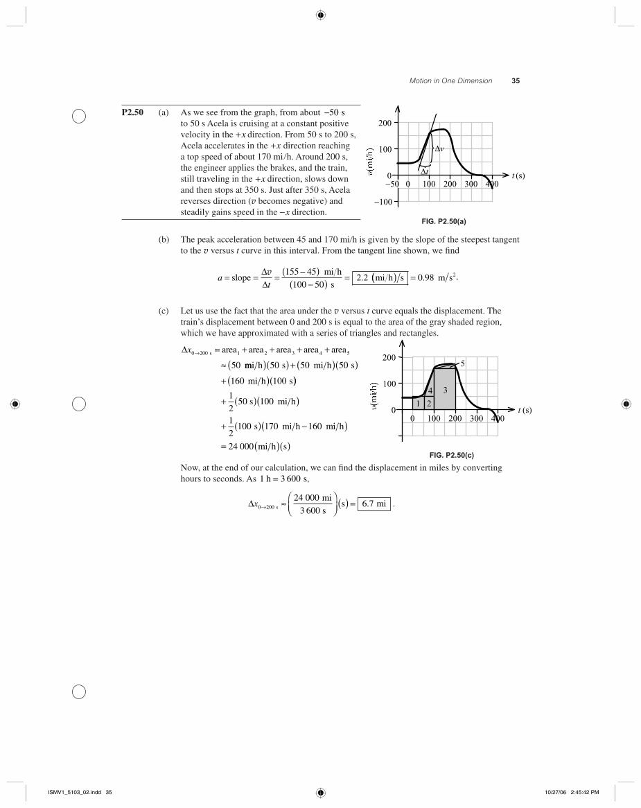
P2.50 (a) As we see from the graph, from about −50 s to 50 s Acela is cruising at a constant positive velocity in the +x direction. From 50 s to 200 s, Acela accelerates in the +x direction reaching a top speed of about 170 mi � h. Around 200 s, the engineer applies the brakes, and the train, still traveling in the +x direction, slows down and then stops at 350 s. Just after 350 s, Acela reverses direction (v becomes negative) and steadily gains speed in the −x direction.

t (s)100 200 300

−100

100

200

400

∆v

∆t

−500

0

FIG. P2.50(a)

(b) The peak acceleration between 45 and 170 mi�h is given by the slope of the steepest tangent to the v versus t curve in this interval. From the tangent line shown, we fi nd

at

= = = −( )−( ) =slope

mi h

smi h

∆∆

v 155 45

100 502 2. (( ) =s m s20 98. .

(c) Let us use the fact that the area under the v versus t curve equals the displacement. The train’s displacement between 0 and 200 s is equal to the area of the gray shaded region, which we have approximated with a series of triangles and rectangles.

∆x0 200

50

→ = + + + +

≈s 1 2 3 4 5area area area area area

mmi h s mi h s

60 mi h s

( )( ) + ( )( )+ ( )(

50 50 50

1 100 ))

+ ( )( )

+ ( ) −

1

2100

1

2100 170 160

50 s mi h

s mi h mii h

mi h s

( )

= ( )( )24 000

Now, at the end of our calculation, we can fi nd the displacement in miles by converting hours to seconds. As 1 3 600 h s= ,

∆x0 200

24 0006 7→ ≈

⎛⎝⎜

⎞⎠⎟

( ) = s

mi

3 600 ss mi. .

t (s)100 200 300

100

200

400

1 2

4 3

5

00

FIG. P2.50(c)


36 Chapter 2

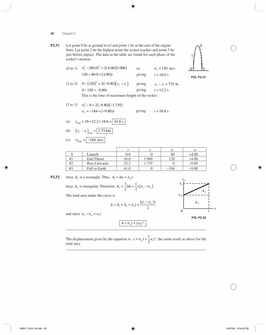
P2.51 Let point 0 be at ground level and point 1 be at the end of the engine burn. Let point 2 be the highest point the rocket reaches and point 3 be just before impact. The data in the table are found for each phase of the rocket’s motion.

(0 to 1) v f2 280 0 2 4 00 1 000− ( ) = ( )( ). . so v f = 120 m s

120 80 0 4 00= + ( ). . t giving t = 10 0. s

(1 to 2) 0 120 2 9 802− ( ) = −( ) −( ). x xf i giving x xf i− = 735 m

0 120 9 80− = − . t giving t = 12 2. s

This is the time of maximum height of the rocket.

(2 to 3) v f2 0 2 9 80 1 735− = −( ) −( ).

v f t= − = −( )184 9 80. giving t = 18 8. s

FIG. P2.51

(a) t total s= + + =10 12 2 18 8 41 0. . .

(b) x xf i−( ) =total

km1 73.

(c) vfinal m s= −184

t x v a0 Launch 0.0 0 80 +4.00

#1 End Thrust 10.0 1 000 120 +4.00#2 Rise Upwards 22.2 1 735 0 −9.80#3 Fall to Earth 41.0 0 −184 −9.80

P2.52 Area A1 is a rectangle. Thus, A hw txi1 = = v .

Area A2 is triangular. Therefore A bh t x xi2

1

2

1

2= = −( )v v .

The total area under the curve is

A A A tt

xix xi= + = +

−( )1 2 2

vv v

and since v vx xi xa t− =

A t a txi x= +v 12

2 .

The displacement given by the equation is: x t a txi x= +v1

22, the same result as above for the

total area.

FIG. P2.52

vx

vx

vxi

0 tt

A 2

A 1



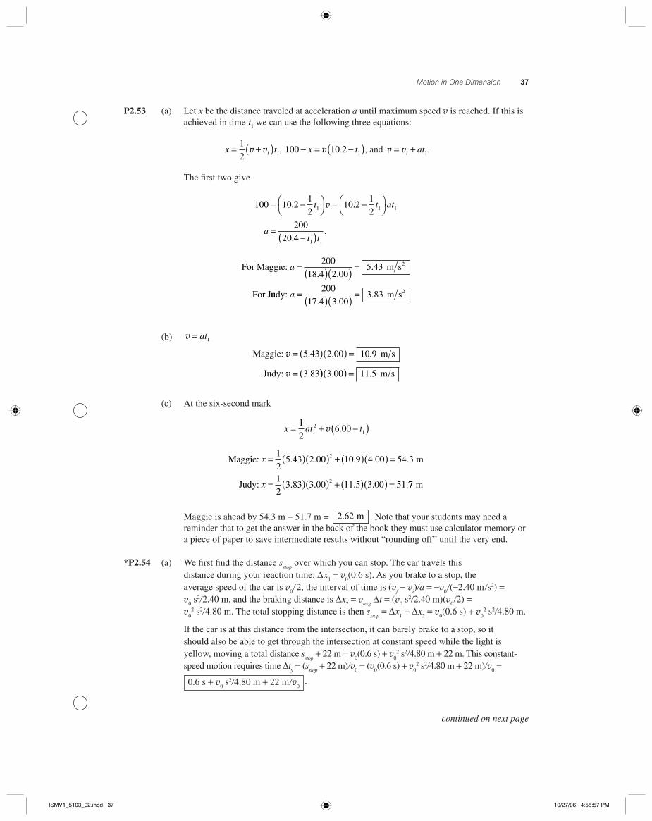
P2.53 (a) Let x be the distance traveled at acceleration a until maximum speed v is reached. If this is achieved in time t1 we can use the following three equations:

x ti= +( )1

2 1v v , 100 10 2 1− = −( )x tv . , and v v= +i at1.

The fi rst two give

100 10 21

210 2

1

2

200

20

1 1 1= −⎛⎝

⎞⎠ = −⎛

⎝⎞⎠

=

. .

.

t t at

a

v

44 1 1−( )t t.

For Maggie: m s

For J

2a = ( )( ) =200

18 4 2 005 43

. ..

uudy: m s2a = ( )( ) =200

17 4 3 003 83

. ..

(b) v = at1

Maggie: m s

Judy:

v

v

= ( )( ) =

= (

5 43 2 00 10 9

3 83

. . .

. ))( ) =3 00 11 5. . m s

(c) At the six-second mark

x at t= + −( )1

26 001

21v .

Maggie: x = ( )( ) + ( )( ) =1

25 43 2 00 10 9 4 00 54 32. . . . . m

Judy: x = ( )( ) + ( )( ) =1

23 83 3 00 11 5 3 00 512. . . . .77 m

Maggie is ahead by 54.3 m − 51.7 m = 2 62. m . Note that your students may need a reminder that to get the answer in the back of the book they must use calculator memory or a piece of paper to save intermediate results without “rounding off ” until the very end.

*P2.54 (a) We fi rst fi nd the distance sstop

over which you can stop. The car travels thisdistance during your reaction time: ∆ x

1 = v

0(0.6 s). As you brake to a stop, the

average speed of the car is v0 � 2, the interval of time is (v

f − v

i)�a = −v

0 �(−2.40 m �s2) =

v0 s2�2.40 m, and the braking distance is ∆ x

2 = v

avg ∆ t = (v

0 s2�2.40 m)(v

0 �2) =

v02 s2�4.80 m. The total stopping distance is then s

stop = ∆ x

1 + ∆ x

2 = v

0(0.6 s) + v

02 s2�4.80 m.

If the car is at this distance from the intersection, it can barely brake to a stop, so it should also be able to get through the intersection at constant speed while the light is yellow, moving a total distance s

stop + 22 m = v

0(0.6 s) + v

02 s2�4.80 m + 22 m. This constant-

speed motion requires time ∆ty = (s

stop + 22 m)�v

0 = (v

0(0.6 s) + v

02 s2�4.80 m + 22 m)�v

0 =

0.6 s + v0 s2�4.80 m + 22 m �v

0 .



38 Chapter 2

(b) Substituting, ∆ty = 0.6 s + (8 m �s) s2�4.80 m + 22 m �(8 m�s) = 0.6 s + 1.67 s + 2.75 s =

5.02 s .

(c) We are asked about higher and higher speeds. For 11 m�s instead of 8 m�s, the time is

0.6 s + (11 m�s) s2�4.80 m + 22 m �(11 m�s) = 4.89 s less than we had at the lower speed.

(d) Now the time 0.6 s + (18 m�s) s2�4.80 m + 22 m�(18 m�s) = 5.57 s begins to increase

(e) 0.6 s + (25 m�s) s2�4.80 m + 22 m�(25 m�s) = 6.69 s

(f ) As v0 goes to zero, the 22 m�v

0 term in the expression for

∆ty becomes large, approaching infi nity .

(g) As v0 grows without limit, the v

0 s2�4.80 m term in the expression for

∆ty becomes large, approaching infi nity .

(h) ∆ty decreases steeply from an infi nite value at v

0 = 0, goes through a rather fl at mini-

mum, and then diverges to infi nity as v0 increases without bound. For a very slowly

moving car entering the intersection and not allowed to speed up, a very long time is required to get across the intersection. A very fast-moving car requires a very long time to slow down at the constant acceleration we have assumed.

(i) To fi nd the minimum, we set the derivative of ∆ty with respect to v

0 equal to zero:

d

dvv

v0

00

10 64 8

22 0..

s +s

mm

s2 2

+⎛⎝⎜

⎞⎠⎟

= +−

44 822 00

2

. mm− =−v

22 m� v02 = s2�4.8 m v

0 = (22m [4.8 m�s2])1�2 = 10.3 m�s

( j) Evaluating again, ∆ty = 0.6 s + (10.3 m�s) s2�4.80 m + 22 m�(10.3 m�s) = 4.88 s , just a little

less than the answer to part (c).

For some students an interesting project might be to measure the yellow-times of traffi c lights on local roadways with various speed limits and compare with the minimum

∆treaction

+ (width�2 � abraking

�)1� 2

implied by the analysis here. But do not let the students string a tape measure across the intersection.

P2.55 a1 0 100= . m s2 a2 0 500= − . m s2

x a t t a t= = + +1 0001

2

1

21 12

1 2 2 22m v t t t= +1 2 and v1 1 1 2 2= = −a t a t

1 0001

2

1

21 12

1 11 1

22

1 1

2

= + −⎛⎝⎜

⎞⎠⎟

+⎛⎝

a t a ta t

aa

a t

a⎜⎜⎞⎠⎟

2

1 0001

211

1

212= −

⎛⎝⎜

⎞⎠⎟

aa

at

1 000 = 0.5(0.1)[1 − (0.1�−0.5)]t12 20 000 = 1.20 t

12 t1

20 000

1 20129= =

. s

ta t

a21 1

2

12 9

0 50026=

−= ≈.

. s Total time = =t 155 s



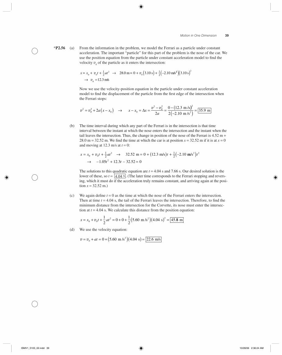
*P2.56 (a) From the in for ma tion in the prob lem, we mod el the Fer ra ri as a par ti cle un der con stant acceleration. The im por tant “par ti cle” for this part of the prob lem is the nose of the car. We use the position equation from the par ti cle un der con stant ac cel er a tion mod el to fi nd the ve loc i ty v

0 of the par ti cle as it en ters the in ter sec tion:

x x t at= + + → = + ( ) +0 0

20

12

12

28 0 0 3 10 2 10v v. . – .m s m/s22 2

0

3 10

12 3

( )( )→ =

.

.

s

m/sv

Now we use the ve loc i ty-po si tion equa tion in the par ti cle un der con stant ac cel er a tionmod el to fi nd the dis place ment of the par ti cle from the fi rst edge of the in ter sec tion when the Fer ra ri stops:

v vv v

02 0

22

0 0

2

22

0 12 3= + −( ) → − = =

−=

− (a x x x x x

a∆

. m /s))−( ) =

2

22 2 1035 9

..

m /sm

(b) The time in ter val dur ing which any part of the Fer ra ri is in the in ter sec tion is that timein ter val be tween the in stant at which the nose en ters the in ter sec tion and the in stant when the tail leaves the in ter sec tion. Thus, the change in po si tion of the nose of the Fer ra ri is 4.52 m + 28.0 m = 32.52 m. We fi nd the time at which the car is at po si tion x = 32.52 m if it is at x = 0 and moving at 12.3 m�s at t = 0:

x x t at t= + + → = + ( ) +0 021

212

32 52 0 12 3 2 10v . . – .m m/s mm/s2 2

21 05 12 3 32 52 0

( )→ + =

t

t t– . . – .

The so lu tions to this quad rat ic equa tion are t = 4.04 s and 7.66 s. Our de sired so lu tion is the low er of these, so t = 4.04 s . (The lat er time cor re sponds to the Fer ra ri stop ping and re vers-ing, which it must do if the ac cel er a tion tru ly re mains con stant, and ar riv ing again at the po si-tion x = 32.52 m.)

(c) We again de fi ne t = 0 as the time at which the nose of the Fer ra ri en ters the in ter sec tion. Then at time t = 4.04 s, the tail of the Fer ra ri leaves the in ter sec tion. Therefore, to fi nd the minimum distance from the in ter sec tion for the Cor vette, its nose must en ter the in ter sec-tion at t = 4.04 s. We cal cu late this dis tance from the po si tion equa tion:

x x t at= + + = + + ( )( ) =0 02 2 21

20 0

1

25 60 4 04 45v . . .m /s s 88 m

(d) We use the ve loc i ty equa tion:

v v= + = + ( )( ) =020 5 60 4 04 22 6at . . .m /s s m/s


40 Chapter 2

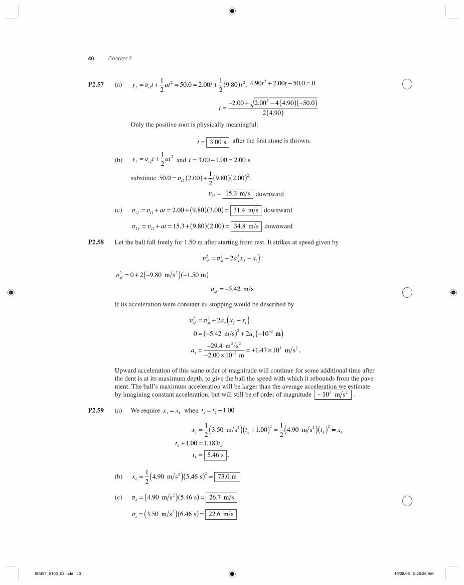
P2.57 (a) y t at t tf i= + = = + ( )v 12 21

250 0 2 00

1

29 80. . . , 4 90 2 00 50 0 02. . .t t+ − =

t =

− + − ( ) −( )( )

2 00 2 00 4 4 90 50 0

2 4 90

2. . . .

.

Only the positive root is physically meaningful:

t = 3 00. s after the fi rst stone is thrown.

(b) y t atf i= +v 221

2 and t = − =3 00 1 00 2 00. . . s

substitute 50 0 2 001

29 80 2 002

2. . . .= ( ) + ( )( )vi :

vi2 15 3= . m s downward

(c) v v1 1 2 00 9 80 3 00 31 4f i at= + = + ( )( ) =. . . . m s downward

v v2 2 15 3 9 80 2 00 34 8f i at= + = + ( )( ) =. . . . m s downward

P2.58 Let the ball fall freely for 1.50 m after starting from rest. It strikes at speed given by

v vxf xi f ia x x2 2 2= + −( ) :

vxf2 0 2 9 80 1 50= + −( ) −( ). .m s m2

vxf = −5 42. m s

If its acceleration were constant its stopping would be described by

v vxf xi x f i

x

a x x

a

2 2

2 2

2

0 5 42 2 10

= + −( )= −( ) + − −. m s mm

m s

mm s

2 22

( )= −

− ×= + ×−ax

29 4

2 00 101 47 102

3.

.. ..

Upward acceleration of this same order of magnitude will continue for some additional time after the dent is at its maximum depth, to give the ball the speed with which it rebounds from the pave-ment. The ball’s maximum acceleration will be larger than the average acceleration we estimate by imagining constant acceleration, but will still be of order of magnitude ~ 103 m s2 .

P2.59 (a) We require x xs k= when t ts k= +1 00.

x t ts k k= ( ) +( ) = ( )( )1

23 50 1 00

1

24 90

2 2. . . m s m s2 2 ==

+ =

=

x

t t

t

k

k k

k

1 00 1 183

5 46

. .

. . s

(b) xk = ( )( ) =1

24 90 5 46 73 0

2. . . m s s m2

(c) vk = ( )( ) =4 90 5 46 26 7. . .m s s m s2

vs = ( )( ) =3 50 6 46 22 6. . .m s s m s2



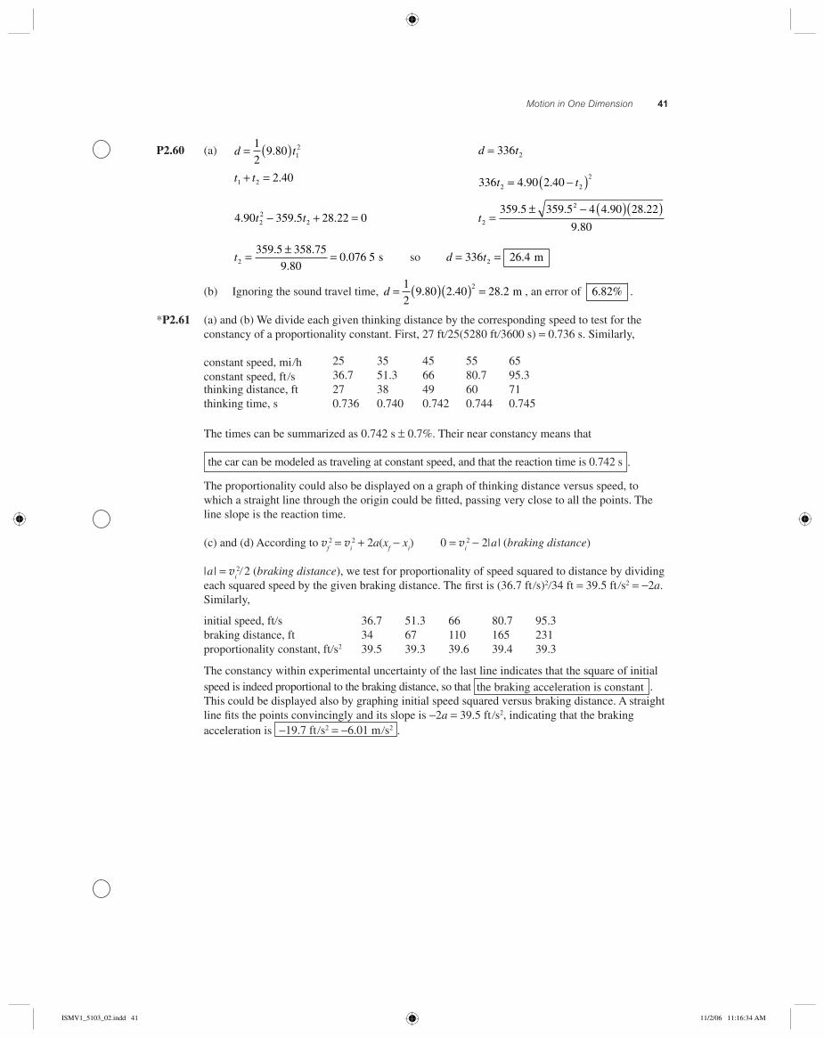
P2.60 (a) d t= ( )1

29 80 1

2. d t= 336 2

t t1 2 2 40+ = . 336 4 90 2 402 2

2t t= −( ). .

4 90 359 5 28 22 022

2. . .t t− + = t2

2359 5 359 5 4 4 90 28 22

9 80=

± − ( )( ). . . .

.

t2

359 5 358 75

9 800 076 5= ± =. .

.. s so d t= =336 26 42 . m

(b) Ignoring the sound travel time, d = ( )( ) =1

29 80 2 40 28 2

2. . . m , an error of 6 82. % .

*P2.61 (a) and (b) We divide each given thinking distance by the corresponding speed to test for the constancy of a proportionality constant. First, 27 ft�25(5280 ft�3600 s) = 0.736 s. Similarly,

constant speed, mi �h 25 35 45 55 65constant speed, ft �s 36.7 51.3 66 80.7 95.3thinking distance, ft 27 38 49 60 71thinking time, s 0.736 0.740 0.742 0.744 0.745

The times can be summarized as 0.742 s ± 0.7%. Their near constancy means that

the car can be modeled as traveling at constant speed, and that the reaction time is 0.742 s .

The proportionality could also be displayed on a graph of thinking distance versus speed, to which a straight line through the origin could be fi tted, passing very close to all the points. The line slope is the reaction time.

(c) and (d) According to vf2 = v

i2 + 2a(x

f − x

i) 0 = v

i2 − 2| a | (braking distance)

| a | = vi2� 2 (braking distance), we test f or proportionality of speed squared to distance by dividing

each squared speed by the given braking distance. The fi rst is (36.7 ft �s)2�34 ft = 39.5 ft �s2 = −2a. Similarly,

initial speed, ft�s 36.7 51.3 66 80.7 95.3braking distance, ft 34 67 110 165 231proportionality constant, ft�s2 39.5 39.3 39.6 39.4 39.3

The constancy within experimental uncertainty of the last line indicates that the square of initial speed is indeed proportional to the braking distance, so that the braking acceleration is constant . This could be displayed also by graphing initial speed squared versus braking distance. A straight

line fi ts the points convincingly and its slope is −2a = 39.5 ft �s2, indicating that the braking acceleration is −19.7 ft �s2 = −6.01 m �s2 .


42 Chapter 2

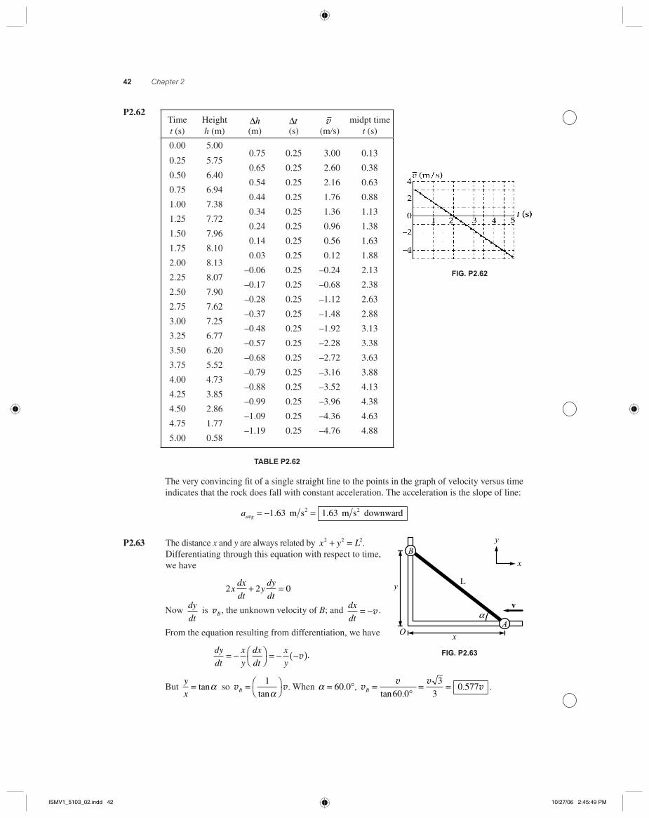
P2.62Time Height ∆h ∆t v midpt timet (s) h (m) (m) (s) (m�s) t (s)

0.00 5.00 0.75 0.25 3.00 0.13

0.25 5.75 0.65 0.25 2.60 0.38

0.50 6.40 0.54 0.25 2.16 0.63

0.75 6.94 0.44 0.25 1.76 0.88

1.00 7.38 0.34 0.25 1.36 1.13

1.25 7.72 0.24 0.25 0.96 1.38

1.50 7.96 0.14 0.25 0.56 1.63

1.75 8.10 0.03 0.25 0.12 1.88

2.00 8.13–0.06 0.25 –0.24 2.13

2.25 8.07–0.17 0.25 –0.68 2.38

2.50 7.90–0.28 0.25 –1.12 2.63

2.75 7.62–0.37 0.25 –1.48 2.88

3.00 7.25–0.48 0.25 –1.92 3.13

3.25 6.77–0.57 0.25 –2.28 3.38

3.50 6.20–0.68 0.25 –2.72 3.63

3.75 5.52–0.79 0.25 –3.16 3.88

4.00 4.73–0.88 0.25 –3.52 4.13

4.25 3.85–0.99 0.25 –3.96 4.38

4.50 2.86–1.09 0.25 –4.36 4.63

4.75 1.77–1.19 0.25 –4.76 4.88

5.00 0.58

TABLE P2.62

The very convincing fi t of a single straight line to the points in the graph of velocity versus time indicates that the rock does fall with constant acceleration. The acceleration is the slope of line:

aa gv = − =1 63 1 63. .m s m s downward2 2

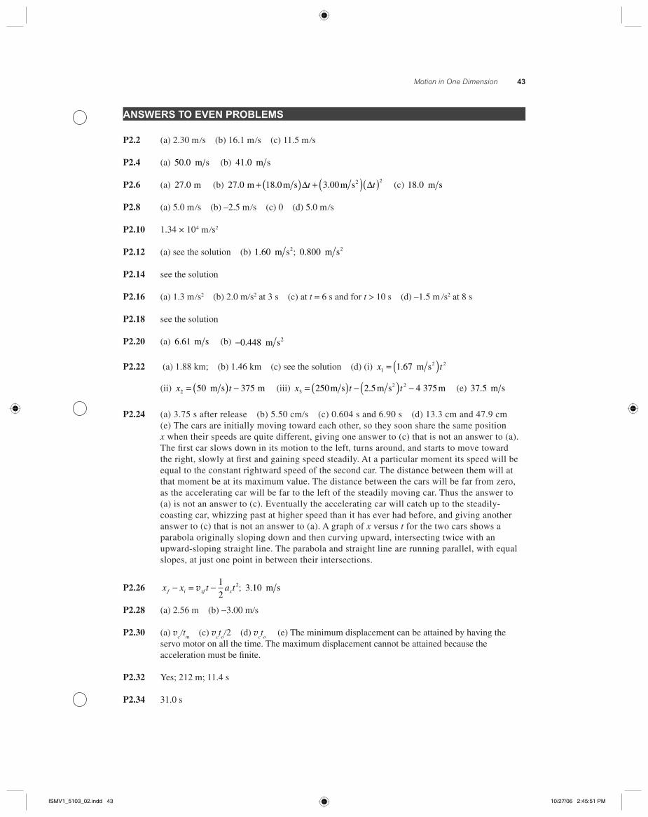
P2.63 The distance x and y are always related by x y L2 2 2+ = .Differentiating through this equation with respect to time, we have

2 2 0xdx

dty

dy

dt+ =

Now dy

dt is vB , the unknown velocity of B; and dx

dt= −v .

From the equation resulting from differentiation, we have

dy

dt

x

y

dx

dt

x

y= − ⎛

⎝⎞⎠ = − −( )v .

But y

x= tanα so v vB = ⎛

⎝⎞⎠

1

tanα. When α = °60 0. , v

v vvB =

°= =

tan ..

60 0

3

30 577 .

FIG. P2.62

FIG. P2.63

B

O

y

α

x

L

v

x

y

A



ANSWERS TO EVEN PROBLEMS

P2.2 (a) 2.30 m �s (b) 16.1 m �s (c) 11.5 m �s

P2.4 (a) 50 0. m s (b) 41 0. m s

P2.6 (a) 27 0. m (b) 27 0 18 0 3 00

2. . . m m s m s2+ ( ) + ( )( )∆ ∆t t (c) 18 0. m s

P2.8 (a) 5.0 m �s (b) –2.5 m �s (c) 0 (d) 5.0 m �s

P2.10 1.34 × 10 4 m �s2

P2.12 (a) see the solution (b) 1 60. m s2; 0 800. m s2

P2.14 see the solution

P2.16 (a) 1.3 m �s2 (b) 2.0 m�s2 at 3 s (c) at t = 6 s and for t > 10 s (d) –1.5 m �s2 at 8 s

P2.18 see the solution

P2.20 (a) 6 61. m s (b) −0 448. m s2

P2.22 (a) 1.88 km; (b) 1.46 km (c) see the solution (d) (i) x t121 67= ( ). m s2

(ii) x t2 50 375= ( ) − m s m (iii) x t t32250 2 5 4 375= ( ) − ( ) −m s m s m2. (e) 37 5. m s

P2.24 (a) 3.75 s after release (b) 5.50 cm�s (c) 0.604 s and 6.90 s (d) 13.3 cm and 47.9 cm (e) The cars are initially moving toward each other, so they soon share the same positionx when their speeds are quite different, giving one answer to (c) that is not an answer to (a). The fi rst car slows down in its motion to the left, turns around, and starts to move toward the right, slowly at fi rst and gaining speed steadily. At a particular moment its speed will be equal to the constant rightward speed of the second car. The distance between them will at that moment be at its maximum value. The distance between the cars will be far from zero, as the accelerating car will be far to the left of the steadily moving car. Thus the answer to (a) is not an answer to (c). Eventually the accelerating car will catch up to the steadily-coasting car, whizzing past at higher speed than it has ever had before, and giving another answer to (c) that is not an answer to (a). A graph of x versus t for the two cars shows a parabola originally sloping down and then curving upward, intersecting twice with an upward-sloping straight line. The parabola and straight line are running parallel, with equal slopes, at just one point in between their intersections.

P2.26 x x t a tf i xf x− = −v1

22; 3 10. m s

P2.28 (a) 2.56 m (b) −3.00 m�s

P2.30 (a) vc �t

m (c) v

cto�2 (d) v

cto (e) The minimum displacement can be attained by having the

servo motor on all the time. The maximum displacement cannot be attained because the acceleration must be fi nite.

P2.32 Yes; 212 m; 11.4 s

P2.34 31.0 s


44 Chapter 2

P2.36 (a) − 0.049 0 m, − 0.196 m, − 0.441 m, with the negative signs all indicating downward (b) − 0.980 m�s, −1.96 m /s, −2.94 m �s

P2.38 1.79 s

P2.40 No; see the solution

P2.42 (a) Yes (b) 3.69 m �s (c) 2.39 m �s (d) +2.39 m �s does not agree with the magnitude of −3.71 m�s. The upward-moving rock spends more time in fl ight, so its speed change is larger.

P2.44 7.96 s

P2.46 (a) and (b) see the solution (c) −4 m s2 (d) 34 m (e) 28 m

P2.48 (a) a = −(10.0 × 107 m �s3) t + 3.00 × 105 m �s2; x = −(1.67 × 107 m /s3) t3 + (1.50 × 105 m �s2)t2 (b) 3.00 × 10 −3 s (c) 450 m �s (d) 0.900 m

P2.50 (a) Acela steadily cruises out of the city center at 45 mi /h. In less than a minute it smoothly speeds up to 150 mi �h; then its speed is nudged up to 170 mi �h. Next it smoothly slows to a very low speed, which it maintains as it rolls into a railroad yard. When it stops, it immediately begins backing up and smoothly speeds up to 50 mi�h in reverse, all in less than seven minutes after it started. (b) 2.2 mi�h�s = 0.98 m�s2 (c) 6.7 mi.

P2.52 vxi xt a t+ 1

22; displacements agree

P2.54 (a) ∆ty = 0.6 s + v

0 s2�4.8 m + 22 m�v

0 (b) 5.02 s (c) 4.89 s (d) 5.57 s (e) 6.69 s (f ) ∆t

y → ∞

(g) ∆ty → ∞ (h) ∆t

y decreases steeply from an infi nite value at v

0 = 0, goes through a rather fl at

minimum, and then diverges to infi nity as v0 increases without bound. For a very slowly moving car

entering the intersection and not allowed to speed up, a very long time is required to get across the intersection. A very fast-moving car requires a very long time to slow down at the constant accelera-tion we have assumed. (i) at v

0 = 10.3 m �s, ( j) ∆t

y = 4.88 s.

P2.56 (a) 35.9 m (b) 4.04 s (c) 45.8 m (d) 22.6 m �s

P2.58 ~103 m �s2

P2.60 (a) 26.4 m (b) 6.82%

P2.62 see the solution; ax = −1 63. m s2


Sm chapter2

Internet

Transcript of Sm chapter2