SLOSHING SIMULATION OF A TANK OSCILLATING TOWARDS …
10
7 ACC JOURNAL 2019, Volume 25, Issue 1 DOI: 10.15240/tul/004/2019-1-001 SLOSHING SIMULATION OF A TANK OSCILLATING TOWARDS MULTIPLE DEGREES OF FREEDOM BY PARTICLE METHOD Shigeyuki Hibi 1 ; Kazuki Yabushita National Defense Academy, Department of Mechanical Systems Engineering, 1-10-20 Hashirimizu, Yokosuka, Kanagawa, 239-8686, Japan e-mail: 1 [email protected] Abstract The tank sloshing problem is very important at design time in LNG/LPG ships. This problem causes impulsive loads to ship structures and is often treated as a non-linear one. In order to estimate these impulsive loads, properly many studies have been carried out through both experimental and numerical approaches. Impulsive pressure on the wall of a tank induced by forced multi-degree oscillations is focused in this research. It is shown in the past authors’ experiment that forced multi-degree oscillations cause stronger impulsive pressure as compared to individual oscillations. Numerical analysis by a particle method based on finite volume technique is introduced in this study to simulate the above phenomena. The suggested particle method is shown to be useful for simulating a strong nonlinear phenomenon. The authors discuss the calculated results of pressure time history with the experimental results. Keywords Sloshing; Impulsive load and pressure; Particle method; Finite volume method. Introduction Sloshing is a phenomenon in which a liquid surface fluctuates violently when a tank with a free surface is shaken at a cycle close to the natural period of the tank. Large impulsive loads may be applied to walls of the tank at this time. In LNG/LPG ships sailing through irregular waves, large impulsive pressure may be generated on the wall near ceiling area when liquid cargo collides to walls of a cargo tank. Then it is important to know the fluctuating pressure caused by sloshing when considering the strength of tank as a structural member in ship design. On the other hand, it is known that a ship navigating through waves has a coupled motion of two degrees of freedom and three degrees of freedom, called longitudinal motion and lateral motion, respectively. For this reason, the hull will fluctuate with a phase difference in some axial direction or rotation direction to those axes. As a result, it is possible that larger sloshing may be caused in tanks inside the ship. In the previous study [1] an apparatus which can oscillate a tank by force was introduced in order to investigate impulsive pressure on the wall of the tank. This apparatus can oscillate it simultaneously towards 3 degrees of freedom (up-down, left-right and rotation) with each phase differences. Through the experiments it was shown larger impulsive pressure could be excited under oscillating the tank simultaneously towards multiple degrees of freedom than under single direction oscillation and the specific phase differences to appear the largest peak values of pressure was identified. In this study the authors verified the results of above experiments by numerical simulation. The authors have developed a particle method [2] with finite volume technique in order to
Transcript of SLOSHING SIMULATION OF A TANK OSCILLATING TOWARDS …

7
ACC JOURNAL 2019, Volume 25, Issue 1 DOI: 10.15240/tul/004/2019-1-001
SLOSHING SIMULATION OF A TANK OSCILLATING TOWARDS MULTIPLE
DEGREES OF FREEDOM BY PARTICLE METHOD
Shigeyuki Hibi1; Kazuki Yabushita
National Defense Academy, Department of Mechanical Systems Engineering,
1-10-20 Hashirimizu, Yokosuka, Kanagawa, 239-8686, Japan
e-mail: [email protected]
Abstract
The tank sloshing problem is very important at design time in LNG/LPG ships. This problem
causes impulsive loads to ship structures and is often treated as a non-linear one. In order to
estimate these impulsive loads, properly many studies have been carried out through both
experimental and numerical approaches. Impulsive pressure on the wall of a tank induced by
forced multi-degree oscillations is focused in this research. It is shown in the past authors’
experiment that forced multi-degree oscillations cause stronger impulsive pressure as
compared to individual oscillations. Numerical analysis by a particle method based on finite
volume technique is introduced in this study to simulate the above phenomena. The suggested
particle method is shown to be useful for simulating a strong nonlinear phenomenon. The
authors discuss the calculated results of pressure time history with the experimental results.
Keywords
Sloshing; Impulsive load and pressure; Particle method; Finite volume method.
Introduction
Sloshing is a phenomenon in which a liquid surface fluctuates violently when a tank with a
free surface is shaken at a cycle close to the natural period of the tank. Large impulsive loads
may be applied to walls of the tank at this time. In LNG/LPG ships sailing through irregular
waves, large impulsive pressure may be generated on the wall near ceiling area when liquid
cargo collides to walls of a cargo tank. Then it is important to know the fluctuating pressure
caused by sloshing when considering the strength of tank as a structural member in ship
design.
On the other hand, it is known that a ship navigating through waves has a coupled motion of
two degrees of freedom and three degrees of freedom, called longitudinal motion and lateral
motion, respectively. For this reason, the hull will fluctuate with a phase difference in some
axial direction or rotation direction to those axes. As a result, it is possible that larger sloshing
may be caused in tanks inside the ship.
In the previous study [1] an apparatus which can oscillate a tank by force was introduced in
order to investigate impulsive pressure on the wall of the tank. This apparatus can oscillate it
simultaneously towards 3 degrees of freedom (up-down, left-right and rotation) with each
phase differences. Through the experiments it was shown larger impulsive pressure could be
excited under oscillating the tank simultaneously towards multiple degrees of freedom than
under single direction oscillation and the specific phase differences to appear the largest peak
values of pressure was identified.
In this study the authors verified the results of above experiments by numerical simulation.
The authors have developed a particle method [2] with finite volume technique in order to

8
stably simulate a fluid phenomenon with strong nonlinearity such as sloshing. At first static
pressure in a tank was verified with the particle method varying the particle number. Next by
comparing the time history of pressure with the experiment result of previous study, the
effectiveness of the proposed particle method was assured.
1 Numerical Analysis Based on Particle Method with Finite Volume Technique
In particle methods, fluid is modeled as a collection of particles and discretized by
considering the interaction between particles without a calculation lattice. Therefore, particle
methods are suitable for intense fluid analysis with strong nonlinearity. Here, we explain the
outline of the particle method proposed by us with finite volume techniques.
The fundamental equations described by a fluid particle coordinates r̂ are represented by the
Navier–Stokes equations and the continuous equation.
(1)
(2)
Here v is the speed of particles, p is the pressure of particles, is the density of fluid, K is
outer forces and is the kinematic coefficient of viscocity of fluid. From Gauss’s theorem
equations (1) and (2) are transformed into flow equations of integral shape.
(3)
(4)
Here n is the normal vector of a particle and V is the volume of a particle.
Eventually, the discretized equations are derived from equations (3) and (4) in the proposed
method.
(5)
(6)
Here

9
(7)
Subscript i means the particle number of interest and subscript j means the neighboring
particle number of the particle i. Superscript n indicates the time step number.
ri means position vector of the i-th particle. The particles are assumed to be spherical (in 2D
model just round) and the influence of the neighboring particle j to the particle i is carried out
through the micro surface area Sij expressed by equation (7) according to the concept of the
Finite Volume Method.
R stands for the radius of a particle and satisfies the following equation.
πR2 = D2 (8)
D is the average inter-particle distance and is determined by the spatial resolution of the
calculation model. This parameter corresponds to the smoothing length h in the SPH[3].
Considering the efficiency and stability of calculation, it is considered that neighboring
particles far from the so called influence radius re do not affect. In this study the following
vallue is adopted for the parameter re.
re = 3.1 D (9)
The pressure value of particles at each time step is obtained by implicitely solving the
equation (6) using the PCGS method The velocity value of particles is also obtained from the
equation (5) implicitly using the PCGS method in case of considering viscosity of fluid and
explicitly in case that viscosity is not taken into consideration.
2 Experimental Apparatus and Condition
2.1 Specification of Oscillation Apparatus
The apparatus used in this study can oscillate a tank attached on the bracket harmonically and
simultaneously towards 3 degrees of freedom with each phase differences (See Fig. 1 and
Table 1).
The size of tank is 400, 400, 100 (mm) (Height, Width, Depth). We define the symbols for the
oscillation directions of 3 degrees of freedom as follows in Fig. 2. Heave oscillation (Up –
down) stands for Z and Sway oscillation (Left – right) stands for X and Roll oscillation
(Rotation) stands for .
A pressure sensor is attached on the right side of the tank mounted on the apparatus. The
position of the sensor is 40 mm from the bottom. The pressure receiver has round area with
diameter of 8mm.
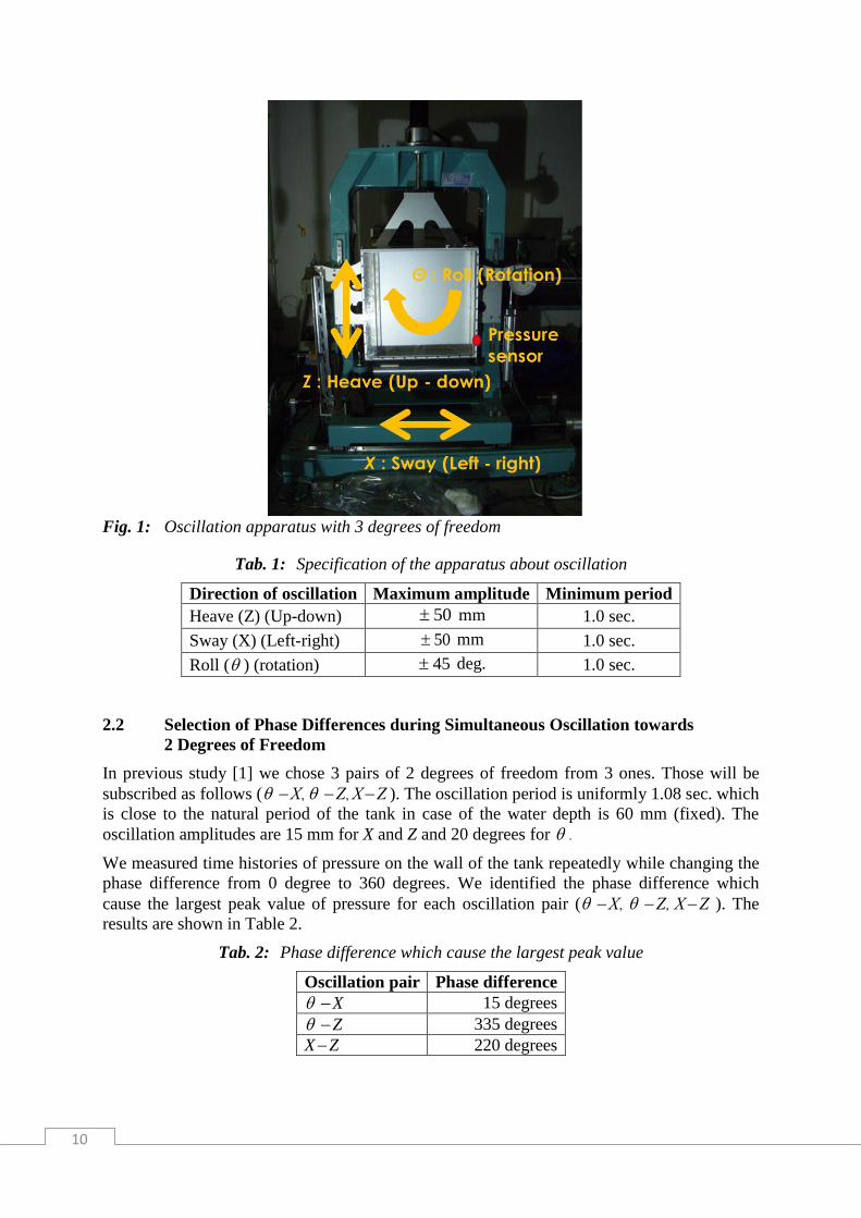
10
Fig. 1: Oscillation apparatus with 3 degrees of freedom
Tab. 1: Specification of the apparatus about oscillation
Direction of oscillation Maximum amplitude Minimum period
Heave (Z) (Up-down) 50 mm 1.0 sec.
Sway (X) (Left-right) 50 mm 1.0 sec.
Roll ( ) (rotation) 45 deg. 1.0 sec.
2.2 Selection of Phase Differences during Simultaneous Oscillation towards
2 Degrees of Freedom
In previous study [1] we chose 3 pairs of 2 degrees of freedom from 3 ones. Those will be
subscribed as follows ( X, Z, XZ ). The oscillation period is uniformly 1.08 sec. which
is close to the natural period of the tank in case of the water depth is 60 mm (fixed). The
oscillation amplitudes are 15 mm for X and Z and 20 degrees for .
We measured time histories of pressure on the wall of the tank repeatedly while changing the
phase difference from 0 degree to 360 degrees. We identified the phase difference which
cause the largest peak value of pressure for each oscillation pair ( X, Z, XZ ). The
results are shown in Table 2.
Tab. 2: Phase difference which cause the largest peak value
Oscillation pair Phase difference
X 15 degrees
Z 335 degrees
XZ 220 degrees

11
3 Numerical Simulation and Discussion
3.1 Comparison of Calculation Accuracy of the Particle Method with Static
Pressure
At first we confirm accuracy of the proposed particle method by static pressure. In Fig. 2 a
tank model used in the above experiment is shown. Water depth is 60mm as in the
experiment. The total particle number is 3,700. The average inter-particle distance D is 38
mm. We define this model of spatial resolution as the base model and name it X1 model. In
addition to this model we prepare 3 additional models named X1/2 (1,500 particles), X2
(10,500 particles), X4 (33,700 particles) model of which D is half, double and 4 times each
other.
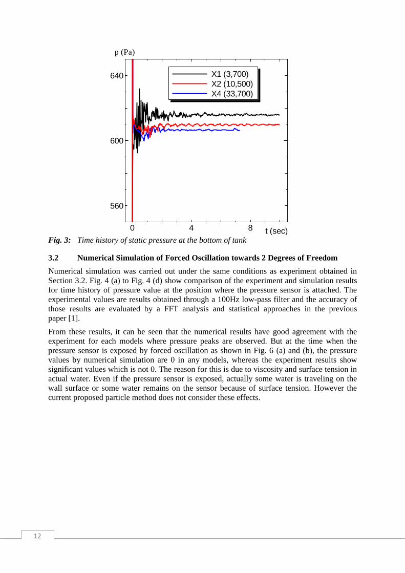
Numerical simulation was carried out with the time step of 0.0001 sec. in all cases. Fig. 3
shows the time history of static pressure at the bottom of tank. In all calculation models we
can see some fluctuations for the first few seconds in simulation time and after that the
pressure values become fairly stable. These fluctuations of pressure occur when relative
position of particles turns more stable and closer from the initial particle arrangement in a
tetragonal lattice.
Fig. 2: Initial particle arrangement for static pressure
Table 2 shows Comparison of static pressure with the theoretical value. It can be seen that the
calculation accuracy is improved according to the spatial resolution.
Tab. 3: Comparison of static pressure with the theoretical value
Simulation result (Pa) Error (%)
X1 616 3.36
X2 610 2.35
X4 607 1.85
12
Fig. 3: Time history of static pressure at the bottom of tank
3.2 Numerical Simulation of Forced Oscillation towards 2 Degrees of Freedom
Numerical simulation was carried out under the same conditions as experiment obtained in
Section 3.2. Fig. 4 (a) to Fig. 4 (d) show comparison of the experiment and simulation results
for time history of pressure value at the position where the pressure sensor is attached. The
experimental values are results obtained through a 100Hz low-pass filter and the accuracy of
those results are evaluated by a FFT analysis and statistical approaches in the previous
paper [1].
From these results, it can be seen that the numerical results have good agreement with the
experiment for each models where pressure peaks are observed. But at the time when the
pressure sensor is exposed by forced oscillation as shown in Fig. 6 (a) and (b), the pressure
values by numerical simulation are 0 in any models, whereas the experiment results show
significant values which is not 0. The reason for this is due to viscosity and surface tension in
actual water. Even if the pressure sensor is exposed, actually some water is traveling on the
wall surface or some water remains on the sensor because of surface tension. However the
current proposed particle method does not consider these effects.
0 4 8
560
600
640 X1 (3,700)
X2 (10,500)
X4 (33,700)
p (Pa)
t (sec)

13
Fig. 4 (a): Time history about X
oscillation.
Fig. 4 (b): Time history about Z
oscillation.
Fig. 4 (c): Time history about XZ
oscillation Fig. 4 (d): Time history about X
oscillation.
Although the peak period and peak value shown in Figures are almost reproduced, the
simulation results show that the pressure values are evaluated to a smaller value as compared
with the experimental values in all models. One reason for this is that relatively low peak
values are considered to be difficult to stand due to numerical viscosity. Another reason is
believed to be due to the relation between the area of the pressure sensor and the special
resolution in the simulation. While the diameter of the pressure sensor is 8 mm, the average
inter-particle distance D is 38 mm in the X1 model and 19 mm in the X2 model. Further study
will be needed for this problem.
4 6 80
1000
2000
Exp.
X2 model
X1 model
Exp.
X2 model
X1 model
t(s)
p(Pa)
4 5 6
0
2000
4000
6000
X2 model
Exp.
X1 modelX2 model
Exp.
X1 model
p(Pa)
t(s)
3 4 5 6
0
1000
2000
Exp.
X2 model
X1 model
p(Pa)
t(s) 4 60
1000
2000
Exp.
X1 model
Exp.
X1/2 model
X1 model
t(s)
p(Pa)

14
Fig. 6 (c): Time history about ZX
oscillation.
3 4 5 6
0
1000
2000
Viscosity
X2 model
X1 model
p(Pa)
t(s)
Fig. 6 (b): Time history about Z
oscillation.
4 5 6
0
2000
4000
6000
X2 model
Viscosity
X1 modelX2 model
Viscosity
X1 model
p(Pa)
t(s) Fig. 6 (a): Time history about X
oscillation.
4 6 80
1000
2000
Viscosity
X2 model
X1 model
Viscosity
X2 model
X1 model
t(s)
p(Pa)
Fig. 5 (b): Moment of exposure of the
pressure sensor about XZ
oscillation.
Fig. 5 (a): Moment of exposure of the
pressure sensor about X
oscillation.

15
In Fig. 4 (d) the numerical result added for the X1/2 model about X is shown. Evenif the
number of particles is just 1,500, it is observed that the accuracy of the analysis is similar.
This shows the superiority of the proposed particle method.
Fig. 6 (a) to Fig. 6 (c) show comparison of the experiment and simulation results considering
fluid viscorsity for time history of pressure value at the position where the pressure sensor is
attached.
From these results, it can be seen that there certainly is a tendency that the pressure
fluctuation becomes looser, such as peak values but even in the case of considering the
influence of the fluid viscosity, there is no big change in the overall pressure fluctuation. This
implies that influence of the fluid viscorsity is limited in the simulation of intense flows like
this study’s experiment even though explicitly taking into consideration and the surface
tension and wettability by that may be much more .important for pressure fluctuation.
Conclusion
In this study the authors carried out numerical simulation of forced oscillation towards
2 degrees of freedom and compared with the previous experimental results. Some
considerations were found about it as below.
Effectiveness of the proposed particle method is shown through the numerical simulation
of intense sloshing phenomena.
In addition to the shape of the pressure sensor, the viscosity of water and the surface
tension on the wall of tank are considered to be related to the pressure fluctuation.
Literature
[1] HIBI, S.: Study on the impulsive pressure of tank oscillating by force towards multiple
degrees of freedom. EPJ Web of Conferences. 2018, Vol. 180, Paper No. 02034.
DOI: 10.1051/epjconf/201818002034
[2] YABUSHITA, K.; HIBI, S: to be posted. Journal of Marine Science and Technology.
[3] MONAGHAN, J. J.: Simulating Free Surface Flows with SPH. Journal of
Computational Physics. 1994, Vol. 110, Issue 2, pp. 399–406.
Shigeyuki Hibi; Kazuki Yabushita

16
SIMULACE ŠPLOUCHÁNÍ NÁDRŽE OSCILUJÍCÍ K VÍCE STUPŇŮM VOLNOSTI METODOU
ČÁSTIC
Problém nárazu nádrže je velmi důležitý ve fázi navrhování lodí LNG / LPG. Tento problém
způsobuje impulzní zatížení lodních struktur a často je považován za nelineární. Za účelem
správného odhadu těchto impulsních zatížení bylo provedeno mnoho studií jak pomocí
experimentálních, tak i numerických přístupů. Tento výzkum se soustřeďuje na impulsní tlak
na stěnu nádrže vyvolaný nucenými vícestupňovými oscilacemi. V předchozím experimentu
se ukázalo, že nucené vícestupňové oscilace způsobují silnější impulzivní tlak ve srovnání
s jednotlivými oscilacemi. V této studii je popsána numerická analýza metodou částic
založená na technice konečných objemů pro simulaci výše uvedených jevů. Navrhovaná
metoda částic se zdá být užitečná pro simulaci silného nelineárního jevu. Autoři srovnávají
vypočtené výsledky časové historie tlaku s experimentálními výsledky.
SIMULATION DES PLÄTSCHERNS DES TANKS ZU EINER MEHRSTUFIGEN
SCHWINGUNG DES SPIELRAUMS MIT DER TEILCHENMETHODE
Das Problem des Anstoßes des Tanks ist in der Phase des Entwurfs von LNG/ LPG-Schiffen
sehr wichtig. Dieses Problem verursacht eine impulsartige Belastung der Schiffsstruktur und
wird oft als nichtlinear betrachtet. Zum Zweck der richtigen Schätzung dieser impulsartigen
Belastungen wurden viele Studien sowohl mit Hilfe von experimentellen als auch
numerischen Ansätzen durchgeführt. Diese Untersuchung konzentriert sich auf den
Impulsdruck an der Wand des Tanks, welcher durch erzwungene mehrstufige Schwingungen
hervorgerufen wurde. Im vorangegangenen Experiment hat sich gezeigt, dass erzwungene
mehrstufige Schwingungen einen stärkeren Impulsdruck im Vergleich mit den einzelnen
Schwingungen erzeugen. In dieser Studie wird die numerische Analyse der Teilchenmethode
beschrieben, welche auf der Technik der endlichen Inhalte für die Simulation der oben
angeführten Erscheinungen basiert. Die vorgeschlagene Teilchenmethode scheint für die
Simulation einer nichtlinearen Erscheinung nützlich. Die Autoren vergleichen die berechneten
Ergebnisse der zeitlichen Historie des Drucks mit den experimentellen Ergebnissen.
SYMULACJA CHLUPANIA ZBIORNIKA OSCYLUJĄCA DO KILKU STOPNI SWOBODY
METODĄ CZĄSTEK
Zagadnienie uderzenia zbiornika jest bardzo ważne na etapie projektowania statków na
LNG/LPG. Problem ten powoduje impulsowe obciążenie struktury statku i często uważany
jest za nieliniowy. W celu prawidłowego oszacowania tych obciążeń impulsowych
przeprowadzono wiele badań opartych na podejściu zarówno doświadczalnym, jak
i numerycznym. W niniejszym badaniu skupiono się na ciśnieniu impulsowym działającym
na ścianę zbiornika, wywołanym wymuszonymi kilkustopniowymi oscylacjami.
Z poprzedniego doświadczenia wynikało, że wymuszone kilkustopniowe oscylacje powodują
większe ciśnienie impulsowe w porównaniu z pojedynczymi oscylacjami. W niniejszym
opracowaniu opisano analizę numeryczną metodą cząstek opartą na technice skończonej
pojemności służącą do symulacji powyżej opisanych zjawisk. Zaproponowana metoda
cząstek wydaje się być przydatna do symulowania silnego zjawiska nieliniowego. Autorzy
porównują obliczone historyczne wyniki ciśnienia z wynikami przeprowadzonych
doświadczeń.