Slippery Tracks: Wheel - Rail Contact - TU/e · PDF fileSlippery Tracks: Wheel - Rail Contact...
10
Slippery Tracks: Wheel - Rail Contact R.I. Popovici and D.J. Schipper Phone +31-(0)53-3892463, e-mail [email protected] University of Twente, Faculty of Engineering Technology, Laboratory for Surface Technology and Tribology, P.O. Box 217, NL 7500 AE Enschede Introduction Low friction due to a bio-film between wheel and rail is generating a security issue in which the braking manoeuvre is failing. Solving this is the biggest priority in railroad industry. Objective The objective of this research is to find a solution to remove the interfacial layer which causes the low friction between wheel and rail. A first step in the process is to predict the coefficient of friction as a function of velocity (Stribeck curve) and as a function of slip or slide to roll ratio (Traction curve) assuming that the interfacial layer behaviour is non-linear viscous. Model A fully deterministic microcontact and friction model was developed for the elliptical contact situation. The present friction model is based on the line contact model developed by Gelinck [1] and the hydrodynamic lubrication model. Inputs In order to get as close as possible to reality, rail and wheel samples were used for a first set of measurements (Figure 1): • Surface roughness (Interferometer, IM); • Coefficient of friction in BL regime (Surface Force Apparatus, SFA). IM SFA IM SFA Figure 1: Measurements of the rail samples. Outputs The main output of the model is the Stribeck curve which describes the variation of the coefficient of friction as a function of velocity. Stribeck curves for 3 types of interfacial layers (water, oil and grease) are presented in Figure 2. 0.23 0.135 0.00 0.05 0.10 0.15 0.20 0.25 0.01 0.1 1 10 100 log v [m/s] Coefficient of friction, f [-] Water Mineral Oil Grease Dry 0.06 20 Figure 2: Stribeck curve for wheel - rail contact. Second result of the model is represented by the evolution of the coefficient of friction with increasing the slip or slide to roll ratio. -0.15 -0.1 -0.05 0 0.05 0.1 0.15 -0.05 -0.03 -0.01 0.01 0.03 0.05 Slip [-] Coefficient of friction, f [-] v=0.1 m/s v=1 m/s v=2 m/s v=3 m/s v=10 m/s Sep Figure 3: Traction curve for wheel - rail contact. Based on these findings the effect of the interfacial layer on the friction level in these contacts is shown to be significant. Future work Introducing the side slip component into the model and viscoelastic behaviour of the interfacial layer. References [1] Gelinck, E.R.M. and Schipper, D.J. (2000), “Calculation of Stribeck Curves for line contacts”, Tribology International, 33, 175-181. Tenth Engineering Mechanics Symposium P-51
Transcript of Slippery Tracks: Wheel - Rail Contact - TU/e · PDF fileSlippery Tracks: Wheel - Rail Contact...

Slippery Tracks: Wheel - Rail Contact
R.I. Popovici and D.J. Schipper
Phone +31-(0)53-3892463, e-mail [email protected] of Twente, Faculty of Engineering Technology,
Laboratory for Surface Technology and Tribology, P.O. Box 217, NL 7500 AE Enschede
IntroductionLow friction due to a bio-film between wheeland rail is generating a security issue inwhich the braking manoeuvre is failing.Solving this is the biggest priority in railroadindustry.
ObjectiveThe objective of this research is to find asolution to remove the interfacial layerwhich causes the low friction betweenwheel and rail. A first step in the process isto predict the coefficient of friction as afunction of velocity (Stribeck curve) and asa function of slip or slide to roll ratio(Traction curve) assuming that theinterfacial layer behaviour is non-linearviscous.
ModelA fully deterministic microcontact andfriction model was developed for theelliptical contact situation. The presentfriction model is based on the line contactmodel developed by Gelinck [1] and thehydrodynamic lubrication model.
InputsIn order to get as close as possible toreality, rail and wheel samples were usedfor a first set of measurements (Figure 1):
• Surface roughness (Interferometer, IM);
• Coefficient of friction in BL regime(Surface Force Apparatus, SFA).
IM SFAIM SFA
Figure 1: Measurements of the railsamples.
OutputsThe main output of the model is the Stribeckcurve which describes the variation of thecoefficient of friction as a function ofvelocity. Stribeck curves for 3 types ofinterfacial layers (water, oil and grease) arepresented in Figure 2.
0.23
0.135
0.00
0.05
0.10
0.15
0.20
0.25
0.01 0.1 1 10 100log v [m/s]
Coeffic
ientoffr
iction,f[-
]
Water
Mineral
OilGrease
Dry
0.06 20
Figure 2: Stribeck curve for wheel - railcontact.
Second result of the model is representedby the evolution of the coefficient of frictionwith increasing the slip or slide to roll ratio.
-0.15
-0.1
-0.05
0
0.05
0.1
0.15
-0.05 -0.03 -0.01 0.01 0.03 0.05
Slip [-]
Coeffic
ientof
fric
tion,f[-
]
v=0.1 m/sv=1 m/sv=2 m/sv=3 m/sv=10 m/s
Sep
Figure 3: Traction curve for wheel - railcontact.
Based on these findings the effect of theinterfacial layer on the friction level in thesecontacts is shown to be significant.
Future workIntroducing the side slip component into themodel and viscoelastic behaviour of theinterfacial layer.
References[1] Gelinck, E.R.M. and Schipper, D.J. (2000),“Calculation of Stribeck Curves for line contacts”,Tribology International, 33, 175-181.
Tenth Engineering Mechanics Symposium P-51
A Computational Approach to Model
Fibre Reinforced Concrete
F.K.F. Radtke, A. Simone and L.J. Sluys
Delft University of Technology
Faculty of Civil Engineering and Geosciences
P.O. Box 5048, 2600 GA Delft
phone +31 15 278 3752, email: [email protected]
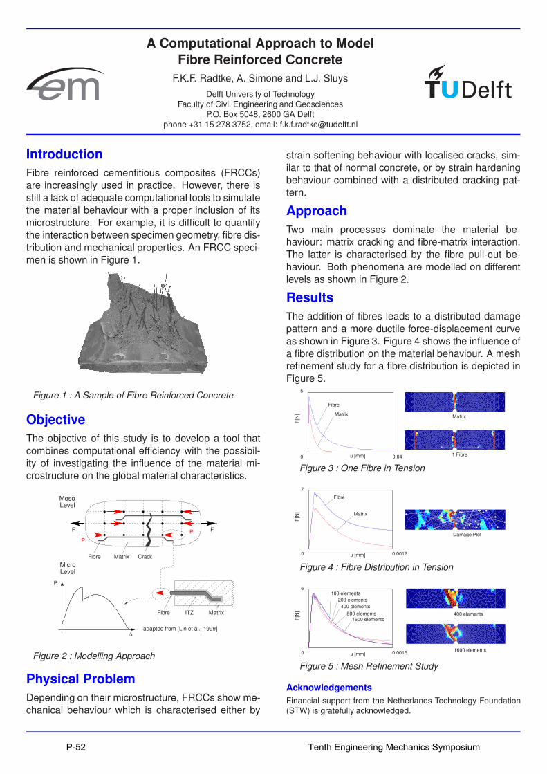
Introduction
Fibre reinforced cementitious composites (FRCCs)
are increasingly used in practice. However, there is
still a lack of adequate computational tools to simulate
the material behaviour with a proper inclusion of its
microstructure. For example, it is difficult to quantify
the interaction between specimen geometry, fibre dis-
tribution and mechanical properties. An FRCC speci-
men is shown in Figure 1.
Figure 1 : A Sample of Fibre Reinforced Concrete
Objective
The objective of this study is to develop a tool that
combines computational efficiency with the possibil-
ity of investigating the influence of the material mi-
crostructure on the global material characteristics.
MesoLevel
MicroLevel
FF
Fibre Matrix Crack
Fibre MatrixITZ
P
P
adapted from [Lin et al., 1999]
P
∆
Figure 2 : Modelling Approach
Physical Problem
Depending on their microstructure, FRCCs show me-
chanical behaviour which is characterised either by
strain softening behaviour with localised cracks, sim-
ilar to that of normal concrete, or by strain hardening
behaviour combined with a distributed cracking pat-
tern.
Approach
Two main processes dominate the material be-
haviour: matrix cracking and fibre-matrix interaction.
The latter is characterised by the fibre pull-out be-
haviour. Both phenomena are modelled on different
levels as shown in Figure 2.
Results
The addition of fibres leads to a distributed damage
pattern and a more ductile force-displacement curve
as shown in Figure 3. Figure 4 shows the influence of
a fibre distribution on the material behaviour. A mesh
refinement study for a fibre distribution is depicted in
Figure 5.5
F[N
]
0 u [mm] 0.04
Fibre
Matrix Matrix
1 Fibre
Figure 3 : One Fibre in Tension
7
F[N
]
0 u [mm] 0.0012
Damage Plot
Fibre
Matrix
Figure 4 : Fibre Distribution in Tension
400 elements
1600 elements
6
F[N
]
0 u [mm] 0.0015
100 elements
200 elements
400 elements
800 elements1600 elements
Figure 5 : Mesh Refinement Study
Acknowledgements
Financial support from the Netherlands Technology Foundation
(STW) is gratefully acknowledged.
P-52 Tenth Engineering Mechanics Symposium

Finite Element Based Reduced Complexity
Analysis of Shells of Revolution
T. Rahman and E.L. Jansen
Delft University of TechnologyFaculty of Aerospace EngineeringP.O. Box 5058, NL 2600 GB Delft
phone +31-(0)15-2782084, email [email protected]
Introduction and objectiveThe current simulation methods (Finite Element computermodels) for nonlinear structural analysis calculations re-quire a lot of effort and expertise from the user, and needa long computer run time. Therefore there is a strong needfirstly for Reduced Complexity intermediate tools that helpin providing a systematic approach to achieve reliable re-sults, and secondly for faster computational tools. Suchtools are not yet available in most of the commercial FEcodes while the research codes that have this capability donot include the important effect of pre-buckling nonlinear-ity. The current research aims at the FE implementationfor Reduced Complexity analysis of shells of revolution in-cluding the pre-buckling nonlinearity effect. Here a singlemode analysis is presented.
Perturbation Methods Reduced Basis Methods
FE based Reduced Complexity Methods
Full model linear analysis
Full model nonlinear analysis
Figure 1 : Reduced Complexity analysis
MethodsKoiter’s perturbation approach that describes the static ini-tial post-buckling path by an asymptotic expansion of thedisplacement field around the bifurcation point form the ba-sis of the present implementation. For a single mode anal-ysis the perturbation expansion of the displacement fieldcan be written as
u = u0 +u1ξ +u2ξ2 +u3ξ
3 + . . . (1)
where u0 is the nonlinear pre-buckling displacement mode,u1 and u2 are the buckling and second order modes, and ξ
is the modal amplitude. Perturbation expansion of the loadparameter λ gives
ξ (λ −λc) = aλcξ2 +bλcξ
3−αλcξ̄ −β (λ −λc)ξ̄ + . . . (2)
where λc is the buckling load, the post-buckling coefficientsa, b, α , and β correspond respectively to the post-bucklingslope, curvature, first, and second imperfection form fac-tors, and ξ̄ is the imperfection amplitude. Once the dis-placement modes and the post-buckling coefficients arecomputed the initial post-buckling path is characterized byequations 1 and 2. This approach has been implemented
for an existing class of curved shell elements in the gen-eral purpose FE code DIANA. The current implementationis largely based on the already existing DIANA implemen-tation and Tiso’s formulation [1].
Results and discussion
An isotropic conical shell representative of the conical in-terstage of the Vega launcher structure has been ana-lyzed. The resulting negative b-coefficient indicate anunstable post-buckling nature and imperfection sensitivity.We observe a fair agreement in the post-buckling coeffi-cients between DIANA and the semi-analytical tool BAAC[2]. A good agreement with full nonlinear analysis is alsoobtained (figure 2). This implementation will be extendedfor multi-mode analysis in near future.
Figure 2 : Reduced Complexity analysis of the Vega launcher:
(a) First buckling mode (b) Second order mode (c) Compari-
son between full and reduced analysis (with imperfection am-
plitude ξ̄ = 0.05t)
Buckling load [N] b α β
BAAC 9.1071×10⁶ -0.44032 0.39031 -0.40697
DIANA 8.9895×10⁶ -0.45524 0.38281 -0.46012
References1. P. Tiso, M. M. Abdalla, and E. L. Jansen. Koiter’s post-buckling anal-
ysis of general shell structures using the finite element method. Inproceedings of the 25th international congress of the aeronauticalsciences, Hamburg, Germany, 2006.
2. G. Zhang. Stability Analysis of Anisotropic Conical Shells. PhD the-sis, Delft University of Technology, 1993.
Tenth Engineering Mechanics Symposium P-53

Strain Path Sensitivity of Mild Steel in
Experiment and Model
M. van Riel, A.H. van den Boogaard
University of Twente/ NIMR
P.O. Box 217, 7500 AE Enschede, The Netherlands
phone +31-(0)53-489 4567, email [email protected]
Material models
In finite element simulations the mechani-
cal behaviour of a material is captured in
a material model that is parame-
terized by some elementary uniax-
ial experiments. However, a deep
drawing process (figure) shows that
the deformation mode is not uniax-
ial and changes during the process.
Sheet metal forming processes are
strongly sensitive to the accuracy
of the material models and therefor
more complex tests and more ex-
tensive models are required.
Goal
The aim of this project is to investigate the mechanical
behaviour of sheet metal under different strain paths
and develop models that describe the observed phe-
nomena.
Experimental observations
During plastic deformation of the material the disloca-
tion structure changes (Figure 2) and causes harden-
ing. After some deformation the dislocation structure
is oriented according the deformation direction
Figure 2: Left: Biaxial tester. Right: Dislocation structure (Mc-
Cabe, Act.Mat. 52(705-714), 2004).
and acts as a barrier for deformations in other direc-
tions. Experiments with a biaxial tester have shown
that a strain path change requires large stresses,
hereby reorienting the dislocation structure with re-
spect to the new deformation direction.
Modelling the mechanical behaviour
The Teodosiu and Hu model is used to describe the
mechanical behaviour of the material. The model is
physically based and calculates the stresses using
the strength of the dislocation structure (S):
S = Sd N ⊗ N + SL
Dependent on the direction of deformation (N) a di-
rectional part (Sd) and a latent part (SL) contribute to
the strength of the dislocation structure.
Results
Results of the experiments and the model are dis-
played in Figure 3. The characteristic overshoot in
stress (σxy) can be qualitatively predicted with this
model.
0 0.1 0.2 0.3 0.4 0.5
0
100
200
300
400
εeq
p (−)
σ (
N/m
m2)
σyy
σxy
σxy
(ref)
0 0.1 0.2 0.3 0.40
50
100
150
200
250
300
350
εeq
p (−)
σ (
N/m
m2)
Sd
SL
σyy
σxy
σxy
(ref)
Figure 3: Experimental (left) and simulation (right) results.
Clearly, the evolution of the yield stress is strongly de-
pendent on Sd, but after the strain path change, Sd is
close to zero and the latent dislocation structure SL
initiates a overshoot in shear stress (σxy).
Future research
• Develop a strategy that determines the material
parameters from experiments.
• Strain rate sensitivity needs to be implemented
in the model, requiring experimental results.
P-54 Tenth Engineering Mechanics Symposium

distribution of dislocation walls in the pile-up. A
qualitative fit to a discrete analysis is shown in
Figure 2. Clearly the solution is inaccurate near
the obstacle.
On the relevance of discreteness in plasticityA. Roy , R.H.J. Peerlings, M.G.D. Geers
Eindhoven University of Technology
Faculty of Mechanical Engineering
P.O.Box 513, NL 5600MB Eindhovenphone +31-(0)40-2473048, email [email protected]
Motivation
Understanding dislocation interactions is
essential in a vast number of industrial
applications. For example: fatigue cracking in
polycrystalline/multiphase materials; micro
scale plasticity; dislocation patterning in metallic
crystals. Popular continuum plasticity theories
account for the long range stress fields of
dislocation distributions accurately but resort to
phenomenology to model the short range
interactions. Local gradients of dislocation
distributions are often used. The questions that
arise are: Is it possible to completely ignore the
underlying discrete nature of dislocation
distributions?
How accurate are the gradient approaches in
modeling short range interactions?
Directional Dependence
An idealized problem of a dislocation pile-up
against a hard obstacle (Figure 1) is rigorously
analyzed and it is seen that the discreteness in
the direction perpendicular to the slip direction
cannot be ignored. Interestingly, “smudging” of
dislocations is allowed in the slip direction [1].
.
Comparison with gradient theories
We compare a gradient dependent Statistical
Mechanics model as formulated in [2] applied to
our problem. The theory predicts an exponential
Reference[1] Roy et al. (2006) Poster EM 2006.
[2] Groma et al. (2003) Acta Mater, 51, 1271-81.
Figure 1. Discrete dislocation representation of a pile-up in an infinite medium. Slip plane separation is “h”. The
red circles represent the immobile wall at x=a.
−∞
∞
2h
h
2h−
h−
0
x a=
y
x
σσσσ
σσσσ
Figure 2. Comparison of discrete analysis of 50 walls of edge dislocations to theory.
Observations and Comment
The theory assumes that characterizing the
nearest neighbor interaction is sufficient in
modeling short range interactions. Figure 4
demonstrates that though the distant walls
individually contribute less to the overall stress
at a dislocation position, the accumulation of the
contributions from these walls is substantial.
This kind of influences is currently lacking in
continuum theories and needs to be looked at.
Figure 4. Stress contributions from every dislocation
wall to the central wall
Tenth Engineering Mechanics Symposium P-55

Towards enrichment of cohesive zone models for
numerical simulation of interfacial delamination
M. Samimi, B.A.E. van Hal, R.H.J. Peerlings,
J.A.W. van Dommelen, M.G.D. Geers
Department of Mechanical Engineering, Eindhoven University of Technology
e-mail: [email protected], Phone: (40) 247 5392, P.O. Box 513, 5600 MB, Eindhoven
Introduction
Interfacial failure, in the form of delamination, is one
of the most prevalent issues in microsystems which
consist of multiple thin and stacked layers (see figure
1). Here, a cohesive zone model (CZM) is employed
for the prediction of delamination.
Figure 1 : Microsystem.
Solution jump problem
Discontinuities in the numerical solutions of rate in-
dependent models are referred to as solution jumps.
This problem can be avoided by sufficiently refining
the mesh, as shown in figure 2.
However, for realistic interface parameters, i.e. small
size of the process zone in brittle interfaces in com-
parison with other dimensions, the element size has
to be extremely small, which results in high computa-
tional costs.
Figure 2 : Double Cantilever Beam (DCB) test [1].
Enriched cohesive zone model
The separation approximation of cohesive zone ele-
ments in the process zone is enriched by a piece-wise
linear function in order to reduce oscillations such as
those observed in the DCB test without need for fur-
ther mesh refinement or application of complicated
path-following approaches (see figures 3,4). The for-
mulation of bulk elements is enriched as well. The
values of crack tip position, a, and enrichment scaling
factors, ht/b, are driven by the deformation process.
Figure 3 : Enrichment of interpolation functions.
Figure 4 : Deformation of an enriched C.Z. element.
Results: mode I delamination
Considering one bulk and one C.Z. element with sep-
aration only in normal direction, the cohesive zone
opening profile is determined by prescribing the crack
tip degree of freedom at fixed positions (see figure 5).
Figure 5 : C.Z. element separation profile for prescribed
crack tip positions.
Conclusions and remarks
• Piece-wise linear enrichment can be used to im-
prove the efficiency and robustness of a CZM.
• Further steps should be taken to complete the
implementation of the proposed enrichment.
References1. B.A.E. van Hal, R.H.J. Peerlings, M.G.D. Geers (2006) Lo-
cal arc-length control method for cohesive zone modelling,
Submitted.
P-56 Tenth Engineering Mechanics Symposium
A Qualitative Study of the Void Formation using Ultrasounds during VARTM
** Special thanks to the US Office of Naval Research and CCM, USA
M.K.Saraswat1,2
1Mekelweg 2, Technical University of Delft,2628 CD Delft, Netherlands.
Email: [email protected] of Composite Materials, University of Delaware,
Newark, DE-19716. USA.
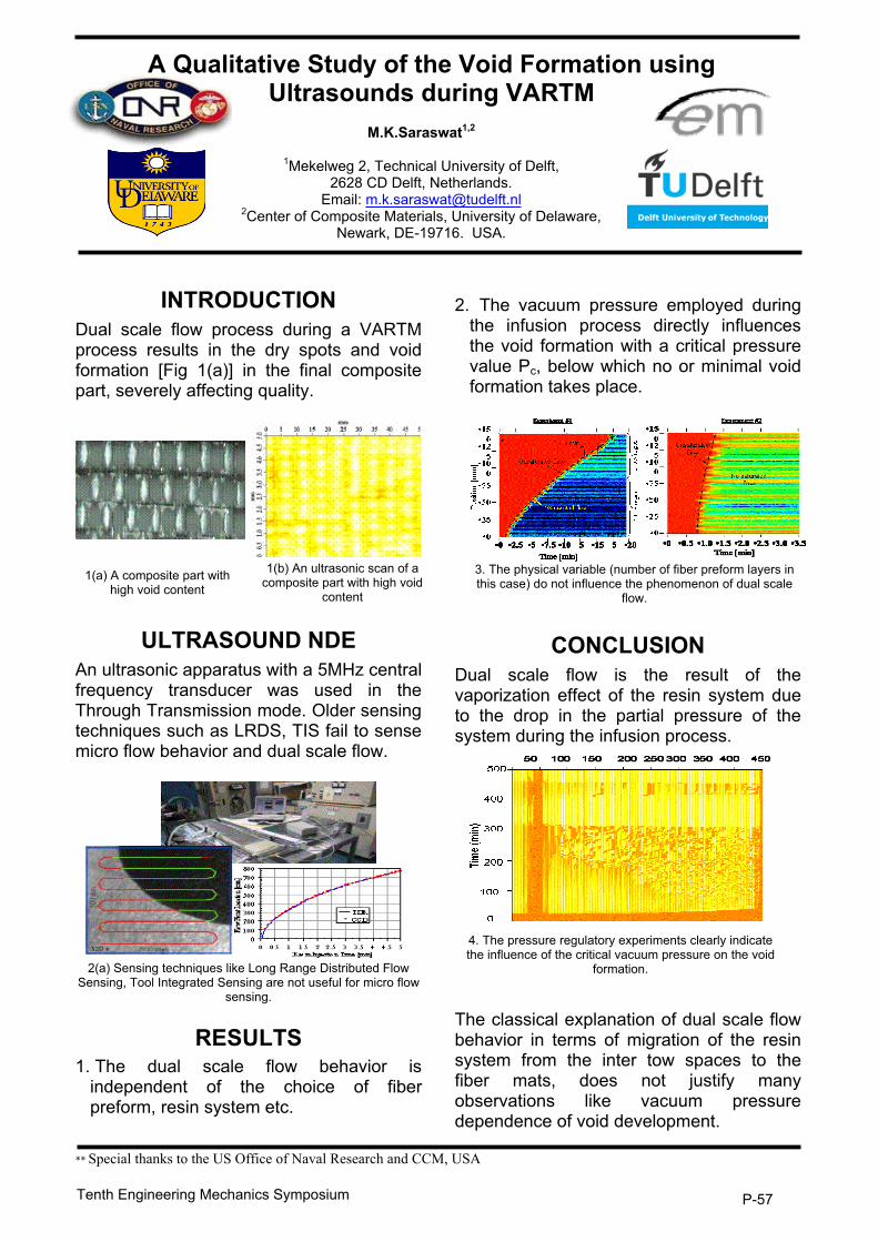
INTRODUCTION
Dual scale flow process during a VARTM process results in the dry spots and void formation [Fig 1(a)] in the final composite part, severely affecting quality.
1(a) A composite part with high void content
1(b) An ultrasonic scan of a composite part with high void
content
ULTRASOUND NDE
An ultrasonic apparatus with a 5MHz central frequency transducer was used in the Through Transmission mode. Older sensing techniques such as LRDS, TIS fail to sense micro flow behavior and dual scale flow.
2(a) Sensing techniques like Long Range Distributed Flow Sensing, Tool Integrated Sensing are not useful for micro flow
sensing.
RESULTS1. The dual scale flow behavior is
independent of the choice of fiber preform, resin system etc.
2. The vacuum pressure employed during the infusion process directly influences the void formation with a critical pressure value Pc, below which no or minimal void formation takes place.
3. The physical variable (number of fiber preform layers in this case) do not influence the phenomenon of dual scale
flow.
CONCLUSION
Dual scale flow is the result of the vaporization effect of the resin system due to the drop in the partial pressure of the system during the infusion process.
4. The pressure regulatory experiments clearly indicate the influence of the critical vacuum pressure on the void
formation.
The classical explanation of dual scale flow behavior in terms of migration of the resin system from the inter tow spaces to the fiber mats, does not justify many observations like vacuum pressure dependence of void development.
Tenth Engineering Mechanics Symposium P-57

Tyre/Road Noise
J.H. Schutte, Y.H. Wijnant, and A. de Boer
Institute of Mechanics, Processing and Control – Twente
Chair of Structural Dynamics and Acoustics, University of Twente
P.O. Box 217, 7500 AE Enschede, The Netherlands
phone +31 53 4893605, email [email protected]
Introduction
Traffic noise is considered to be an important
environmental problem, leads to annoyance and
even health damage. The interaction between the
tyre and road surface causes tyre vibrations and
air displacements, by which sound is generated
(figure 2). Today tyre/road noise is the dominant
noise source for driving speeds exceeding 40 km/h
(figure 1).
Figure 1 : Will tyre/road noise be dominant now?
The introduction of porous road surfaces has reduced
tyre/road noise significantly. After some years,
however, the sound reduction is decreased because
of pollution of the porous layer. Noise reduction
can also be accomplished by optimization of the
tyre. Simplified tyre models have been developed,
which suffer from limited accuracy. Finite element
models are more accurate, but computationally very
expensive at high frequencies.
air-pumping
impact
slip-stick
resonances
rotationradial and tangential vibrations
road
tyre
Figure 2 : Mechanisms of tyre/road noise generation.
Objective
The aim of this research is to develop a numerical
model, which is sufficiently fast to quantitatively
predict tyre/road noise by means of a direct contact
approach.
Methods
The tyre will be modelled by means of finite elements,
suitable for large deformations and anisotropic
material behaviour [1].
The contact will be modelled in the time domain,
because of the inherent non-linearity. A direct contact
approach [2] is used to model the contact between
tyre and road. The convergence is good and friction
between tyre and road is accounted for.
The boundary element method [3] will be used to
calculate the radiated sound from the tyre vibrations.
The road’s influence is taken into account. A
preliminary result is given in figure 3.
1050HzdB
60
70
80
90
100
110
120
Figure 3 : Sound pressure level at 1050 Hz of a slick
tyre on a flat, acoustic hard road (the tyre rolls to the
right) [2].
References1. Ten Thije, R.H.W. et al. (2007) Computer Methods in Applied
Mechanics and Engineering, 196, 3141–3150.
2. Wijnant, Y.H. and de Boer, A. (2006) Proceedings of
ISMA2006, Leuven, Belgium.
3. Visser, R. (2004) PhD thesis, University of Twente,
Enschede, The Netherlands.
The support of TNO and Vredestein within this CCAR project is
gratefully acknowledged. a
P-58 Tenth Engineering Mechanics Symposium
Thermal effects on two-phase flow in porous media
Xuming Shan1, Tim C. Hooijkaas1, Cor van Kruijsdijk2 and Garth N. Wells3
1Delft University of Technology2Royal Dutch Shell
3University of Cambridgeemail: [email protected]
IntroductionIn thermal recovery processes, heated water or steam isinjected into a reservoir to stimulate oil production. Thisprocess has been modelled numerically in order to de-velop improved insights into the recovery of heavy oil. Thecomplexity of the problem presents numerous modellingand numerical challenges.
Here we simulate temperature-dependent two-phase flowin porous media and invoke the Boussinesq approxima-tion to model buoyancy effects. Using the FEniCS frame-work (www.fenics.org), the development of the compu-tational model has been automated.
ApproachTemperature-dependent two-phase immiscible flow, as-suming incompressibility of the fluids, is governed by:
• Darcy’s law for each phase
vα =krα k
µα
(−∇pα + ραg)
• Pressure equation
∇ ·
((krw
µw
+kro
µo(T )
)k ·∇p−
(krwρw
µw
+kroρo
µo(T )
)k ·g
)= f
• Saturation equation
∂S
∂ t+ v ·∇ f (S) = 0,
where v = vw + vo, and f (S) is the water fractionalflow function, given by
f (S) =krw/µw
krw/µw + kro/µo(T )
• Heat transfer
∂T
∂ t+ v ·∇T −∇ ·α∇T = 0
where S is water saturation, p is the pressure, T is temper-ature, k is the permeability, krα is the relative permeabilityof phase α, which is a funcition of water saturation. µα isthe viscosity of α phase, with µo being temperature depen-dent, since we are considering thermal recovery methodsof heavy oil. The capillary pressure has been neglected.
A finite element method is used, with upwinding in the formof the Streamline Upwind Petrov-Galerkin (SUPG) methodand a residual-based shock capturing operator.
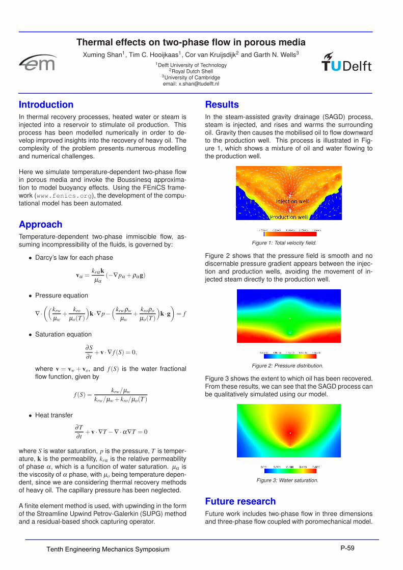
Results
In the steam-assisted gravity drainage (SAGD) process,steam is injected, and rises and warms the surroundingoil. Gravity then causes the mobilised oil to flow downwardto the production well. This process is illustrated in Fig-ure 1, which shows a mixture of oil and water flowing tothe production well.
Figure 1: Total velocity field.
Figure 2 shows that the pressure field is smooth and nodiscernable pressure gradient appears between the injec-tion and production wells, avoiding the movement of in-jected steam directly to the production well.
Figure 2: Pressure distribution.
Figure 3 shows the extent to which oil has been recovered.From these results, we can see that the SAGD process canbe qualitatively simulated using our model.
Figure 3: Water saturation.
Future research
Future work includes two-phase flow in three dimensionsand three-phase flow coupled with poromechanical model.
Tenth Engineering Mechanics Symposium P-59

The competition between solid-state phase
transformations and plastic deformation:
discrete interfaces and discrete dislocationsJ. Shi1, S. Turteltaub1, J. J. C. Remmers1, E. van der Giessen2
1 Delft University of Technology, Aerospace Engineering
Kluyverweg 1, 2629HS Delft, The Netherlands2 University of Groningen, Applied Physics, Materials Science Center
Nijenborgh 4, 9747AG Groningen, The Netherlands
Introduction
Steels assisted by transformation induced plasticity
(TRIP) are a class of high strength-high ductiltiy mate-
rials. During mechanical loading, TRIP steels gain ad-
ditional strength due to a martensitic transformation.
This phenomenon is strongly coupled to plastic defor-
mations in the austenitic matrix. In order to optimize
the mechanical properties of these materials, it is im-
portant to understand the coupling of the transforma-
tion and plasticity.
Method
The coupled transformation-plasticity problem is de-
composed into three sub-problems (see figure 1):
u 0
t0
boundaryconditions complementary
boundary conditions
= + +
Actual Field Martensitic Field Dislocation Field Complementary Field
Figure 1 : Decomposition of coupled problem
• A transformation problem for individual marten-
sitic plates that can be solved using Eshelby’s
inclusion theory and Mushkelishvili’s potentials.
• A plasticity problem for individual dislocations,
based on the discrete dislocation method [1].
• A complementary problem to account for polar-
ization stresses and actual boundary conditions.
This problem is solved using FEM.
Results
One polycrystal tensile case was simulated to illus-
trate the interaction between martensitic transforma-
tion and plastic deformations. The specimen has a
total of 37 grains with arbitrary polygonal shapes. Two
tensile cases were analyzed as follows:
• Case 1: a benchmark simulation where all
grains correspond to the ferrite phase
• Case 2: a multiphase simulation with four
austenitic grains embedded in a ferritic matrix.
+
+++
+ +
++++
+
+++
+ ++ ++
++++
+
++++
+
+
+
++
Case 1: Ferrite only
σxx (MPa)
+
++++
+
++
+
+++
+
+
+++ +
+
+++ ++++
+ ++++
+
++++
++++ +++
++++
+++ + ++
+ ++++ + +
++++
++++++++++++ ++++++ +
+++++
++++
+++ +++++ +++++++++ + + +
+++ +++ + +
+++++++ ++
++++
+
+ + + +++ ++
++++
+
+++ +
++++
++
+
+
+ +++++
+
++ +
+
+
+++++ ++++
+
++++++++++ +++ +
+ +++ +++++ +
++
+
++++
+++
+++ +++
+++
+ +++++
+++
+
++ ++
+ ++
+
+
++
++
++ +
+ ++++
+
++
+++
+
+
+
+
+
+
+++ +
+++++
+
+++
+ +
+
+
+
+
+++
++++++
++
+
+++
+
+
++
++
+
++
++
++
+
+
++
+
++
++
++
+
+++
++
+
+++++
+++++ ++
+
+ +
++
+
+
++
+
+
++
+
++
++++
++
+
++ +++
++ ++
+
+
+
+
+
++
+
++ ++
++
+
+
+ +
+
+++
+
++
++
+
+
+
++
+++
++++
+
++
+++
+
++
+
++
++
+
++
++
++
++
+++
+
++
++
+
++
+++
+
+++
+
+++
++
+
+++
+
++
+
+
++
++
++
+
+
+ ++
+++
+
+++
+
+
+
+
+++++ ++++
+ +
++++++
+++
++
++++
+
+
++
+
+
+ +
+
+
+ +
++
++
+
+
+
+
++
+ + +
+
+++
+
+
+
++
++
+
+
+
++
++
+++
+
+
++ ++
++
+
+++
++
+
++++
+
+
+++
+
+++
+
+
++
++
+
++++
+
++
++
+
+
+
+++
+
+++
+
++
++ +++
+
+
++
+
+
+
++
+
++
+
+
+
+
++
+
+
+
++
+
+
++
++++
+
+ ++
+
+
+
+
+
+ +
+
++ +
+
+
+++
+
+++
++
+
+
+++
++ +
+++ +
+
+
+
++++
++++
+
++ ++
+
+ + +
++
+
+
++++
+
+
+++++
++ +
++
+++++
++
+++++
++++++
+
+
+
+++
+++
++++
+
++ ++
+
++
++ +
+
+
+
++ +
++
++++ ++
+
+
+
+
+
++ ++
++
+
++
+
+++
+
++
++
++
+
++
+
++
+
+
++
+
+
+
+
+
+
+
++
++
+
+++
+
++
++
+
+
+
+
+
+
+
+
+
+
+++
+
+
+
+
+
++
+
++
++
++
+
+
+++
++++ ++ +++
+
+
+
+
+ +++
+ ++++
+
++
+ +
++
+
++++++
+ +
++
+
+
+
+
++
+
+
+
+
+
++
+
+++ + +++
++
+
+ +++++
+ ++++
++
+
+++ +++
+++
++
+
+
+++ +
++
++
+++
++++
+
+
+
+
+++++
++
++
+ +
+ +
++
+
++
+
+
+
+++
+
+
+
+
++ +++ ++ ++
++
++ ++
+
+
++
+++
+ ++
+
+
+
+
+
+
++ +
+
++++
+
+++
+
++
+
++++
+
+
+
+++++
+
+
+
++
+++
++
+ + +
+++
++++
+
+++
+++
++++
+ +
++
+
+
++
++
+
+
++++++
++
++
++
+
++ +
+
++
+
+
+
+
+++
+
+
++
+++++ +
+++
++
+
+
+
++
+
++
+
+
+++++
+
++
++
++
+
+
+
+
+
++
++
++ +
+
++
+
++++
+
+
+++
+
+
++ +
+
+
+
++
++
+
+++
++
++
+
++
+
++++ +
+
+
++
++
++
+
++
++
+++++++
++
++
+
+
++++
++
++++
++ +
++
+ +
+
++++
++ ++
+ +++++++++
++++ +
+++ ++++
+
++
++++++ +
+
++ ++ ++
+
+ ++ ++ ++
+ +
+
+ + +
+
+
+
+++
+
+
+
+++
+++
+
500
400
300
200
100
0
100
200
300
400
500
Case 2: Ferrite and austenite
Figure 2 : Contour plots of axial stress σ11 when ǫ11 = 0.1%
Figure 2 shows the distribution of dislocations (cases
1 and 2) and distribution of martensitic plates (case 2)
for ǫ11 = 0.1%. Three out of the four austenitic grains
have partially transformed into martensite. For case
2, it can been seen that the martensitic transformation
that occurs in the austensitic grains is accommodated
by a significant plastic deformation in the surrounding
ferrite. In contrast, the benchmark simulation (case
1) shows a limited number of dislocations due to the
external loading.
Strain
Ma
rte
nsitic
vo
lum
efr
actio
n
0.0004 0.0006 0.0008 0.0010
0.02
0.04
0.06
0.08
0.1
Martensitic volume fraction (case 2)
Strain
Dis
loca
tio
nD
en
sity
0.0004 0.0006 0.0008 0.0010
10
20
30
40
50
Ferrite only (case 1)AusteniteFerrite (case 2)
Figure 3 : Dislocation density and martensitic volume fraction
The evolution of the volume fraction of martensite for
case 2 and the change in dislocation density for cases
1 and 2 as functions of the axial strain are shown in
figure 3. The graphics indicate that sudden increases
in the number of dislocations tend to slow down the
transformation process. This is related to a reduction
in the transformation driving force due to plastic dissi-
pation in the surrounding ferrite.
References1. Van der Giessen, E., Needleman, A., (1995) Modelling Simul. Mater.
Sci. Eng., 3: 689-735.
P-60 Tenth Engineering Mechanics Symposium