Slip line analysis of heterogeneous flawed welds loaded...
150
Filip Van Gerven in tension Slip line analysis of heterogeneous flawed welds loaded Academic year 2014-2015 Faculty of Engineering and Architecture Chairman: Prof. dr. ir. Patrick De Baets Department of Mechanical Construction and Production Master of Science in Electromechanical Engineering Master's dissertation submitted in order to obtain the academic degree of Counsellor: Ir. Koen Van Minnebruggen Supervisors: Prof. dr. ir. Wim De Waele, Dr. Stijn Hertelé
Transcript of Slip line analysis of heterogeneous flawed welds loaded...

Filip Van Gerven
in tensionSlip line analysis of heterogeneous flawed welds loaded
Academic year 2014-2015Faculty of Engineering and ArchitectureChairman: Prof. dr. ir. Patrick De BaetsDepartment of Mechanical Construction and Production
Master of Science in Electromechanical EngineeringMaster's dissertation submitted in order to obtain the academic degree of
Counsellor: Ir. Koen Van MinnebruggenSupervisors: Prof. dr. ir. Wim De Waele, Dr. Stijn Hertelé

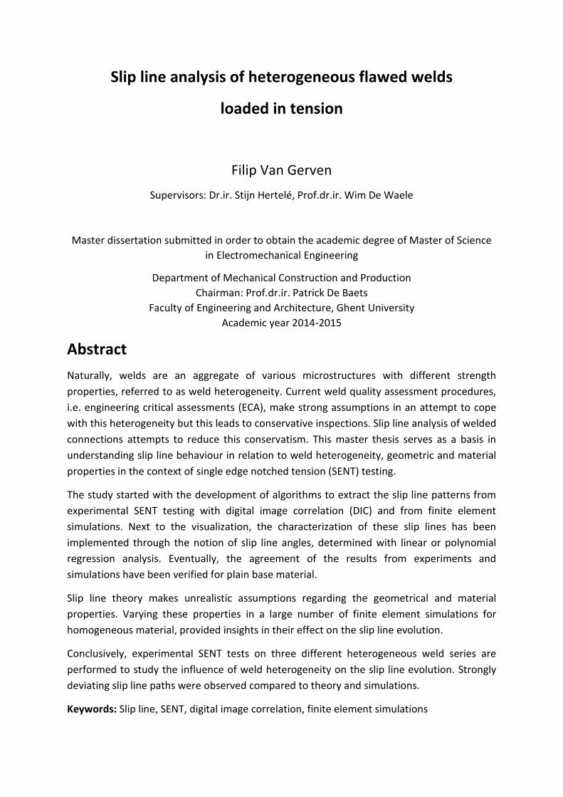
Preface
This master thesis is the keystone of my engineering education at Ghent University. It has been
a real pleasure being part of the research group for the past year while accomplishing the
most intensive and challenging task of my education. Every single member of the laboratory
made me feel welcome and was happy to be helpful. Especially, I would like to express my
sincere gratitude to the following people:
First, I would like to thank my supervisor Stijn Hertelé for his strong support throughout the
year. His persistent drive to help me with this demanding task was eminent. I also thank Prof.
Wim De Waele for his constant availability and counseling.
The technical staff of Soete Laboratory and Belgian Welding Institute are acknowledged for
their technical support throughout the year. More specifically, I would like to thank Johan Van
Den Bossche for the preparation of the SENT specimens, Chris Bonne for the electrical support,
Hans Van Severen for the technical support and Gert Oost for the post mortem embedment
of the SENT specimens.
Thanks to all of you!
Filip Van Gerven, Ghent, June 2015
The author and supervisors give permission to make this master dissertation available for
consultation and to copy parts of this master dissertation for personal use. In the case of any
other use, the copyright terms have to be respected, in particular with regard to the obligation
to state expressly the source when quoting results from this master dissertation."
Supervisors
Prof. dr. ir. W. De Waele, Dr. S. Hertelé
Counsellor
Ir. K. Van Minnebruggen
Author
Filip Van Gerven
Slip line analysis of heterogeneous flawed welds
loaded in tension
Filip Van Gerven
Supervisors: Dr.ir. Stijn Hertelé, Prof.dr.ir. Wim De Waele
Master dissertation submitted in order to obtain the academic degree of Master of Science
in Electromechanical Engineering
Department of Mechanical Construction and Production
Chairman: Prof.dr.ir. Patrick De Baets
Faculty of Engineering and Architecture, Ghent University
Academic year 2014-2015
Abstract
Naturally, welds are an aggregate of various microstructures with different strength
properties, referred to as weld heterogeneity. Current weld quality assessment procedures,
i.e. engineering critical assessments (ECA), make strong assumptions in an attempt to cope
with this heterogeneity but this leads to conservative inspections. Slip line analysis of welded
connections attempts to reduce this conservatism. This master thesis serves as a basis in
understanding slip line behaviour in relation to weld heterogeneity, geometric and material
properties in the context of single edge notched tension (SENT) testing.
The study started with the development of algorithms to extract the slip line patterns from
experimental SENT testing with digital image correlation (DIC) and from finite element
simulations. Next to the visualization, the characterization of these slip lines has been
implemented through the notion of slip line angles, determined with linear or polynomial
regression analysis. Eventually, the agreement of the results from experiments and
simulations have been verified for plain base material.
Slip line theory makes unrealistic assumptions regarding the geometrical and material
properties. Varying these properties in a large number of finite element simulations for
homogeneous material, provided insights in their effect on the slip line evolution.
Conclusively, experimental SENT tests on three different heterogeneous weld series are
performed to study the influence of weld heterogeneity on the slip line evolution. Strongly
deviating slip line paths were observed compared to theory and simulations.
Keywords: Slip line, SENT, digital image correlation, finite element simulations

Slip line analysis of heterogeneous flawed welds
loaded in tension
Filip Van Gerven
Supervisors: Dr. Ir. Stijn Hertelé, Prof. Dr. Ir. Wim De Waele
Abstract –To obtain better insights into the slip line evolution in
heterogeneous welds, algorithms have been developed to extract
and characterize slip lines in single edge notched tension (SENT)
specimens. The algorithm has been implemented both for SENT
testing in an experimental setup, as for finite element SENT
simulations. Compliance of both methods is validated and
extensive experimental and numerical experiments are performed
to study the interaction between slip line behaviour, weld
heterogeneity and material properties.
Keywords: Slip line, SENT, DIC, finite element analysis
I. INTRODUCTION
Due to the rising demand for energy resources worldwide
pipeline installation in harsh environments becomes the new
standard. Naturally, welds are an aggregate of various
microstructures with different strength properties, referred to
as weld heterogeneity. As welding generally introduces flaws
into the structure, each connecting girth weld is judged for its
quality through an Engineering Critical Assessment (ECA).
However, due to the complex nature of the weld, current ECA
procedures make strong assumptions regarding the weld
properties, leading to conservative inspections. The slip line
study aims at reducing the conservatism of these procedures.
II. WELD HOMOGENIZATION
In practice, a heterogeneous weld is translated to a
homogeneous equivalent through a homogenization procedure.
Soete Laboratory has proposed a homogenization model,
named “UGent model” in that perspective. The model uses the
concept of slip lines in the material. Slip line theory is a
branch of plasticity theory, expressing the paths of maximum
shear strain in a homogeneous rigid-perfectly plastic material.
The theory has been established both for plane strain and
plane stress conditions. Theoretical solutions are derived for
some simplified analytical cases, such as slip lines at stress
free surfaces (45° for plane strain, 56.5° for plane stress).
III. SLIP LINE ANALYSIS
The theoretical background of slip line theory for plane
strain conditions is established at the start of this thesis. From
these theoretical concepts, an algorithm is established to locate
slip lines both in single edge notched tension (SENT)
experiments analyzed with digital image correlation (DIC), as
finite element SENT simulations. Hereto, a numerical grid is
applied on the SENT specimen as displayed in figure 1 left
and the location of maximum shear strain is determined at
each horizontal array of grid points. Those maxima will
constitute the slip lines at both sides of the notch, see figure 1
right. The coordinates of these maxima can be calculated
according to either the deformed shape of the specimen or its
initial shape. Next to visualizing the lines, the slip line
evolution is characterized through regression analysis. Two
regression strategies have been elaborated: linear regression
and polynomial regression. Linear regression fits a straight
line, while polynomial regression fits a polynomial with a
user-dictated degree to each slip line separately (above and
below the notch, figure 1). From these regression lines, slip
line angles are determined with respect to the Y-axis. With
linear regression, one angle results for each slip line, while
with polynomial regression numerous angles can be extracted
along the slip line by evaluating its derivative at the desired
locations.
Y
X
F
F
Side groove notch
grid
Y
X
F
F
Lin. Reg.
Pol. Reg.
Figure 1: Determine the slip lines in a SENT specimen
The compliance of the experimental and numerical results
obtained with this algorithm was positively evaluated with two
‘dummy’ experiments on plain base metal specimens and the
simulation of both in finite element software.
IV. SENT EXPERIMENTS
To link weld heterogeneity with slip line evolution, three
welds have been SENT tested. Each weld has a different
heterogeneous nature. Strain patterns at the surface have been
tracked with DIC.
Figure 2: Slip lines visualized with DIC

V. SENT SIMULATIONS
Slip line theory assumes a homogeneous rigid-perfectly
plastic material in plane strain or plane stress conditions.
However, steel has elastic and strain hardening properties and
loading conditions differ from theoretical plane strain and
plane stress. To investigate the difference of theoretical slip
line behavior with that for realistic material properties and
loading conditions, 96 finite element simulations have been
performed on two-dimensional and three-dimensional side
grooved SENT specimens. As reported in table 1, the
following parameters were varied: Ramberg-Osgood strain
hardening exponent n, Young’s modulus E, the initial crack
depth a0/W and the specimen geometry. Four different
geometries are simulated: 2D plane strain and plane stress and
3D SENT specimens with cross sections B = W and B = 2W.
Note that n = 500 aims to describe a perfectly plastic material,
while E = 20000 GPa intents to model a rigid material.
Table 1: Varied parameters over the simulations
Geometry n [-] E [GPa] a0/W [-]
Plane strain
10, 15,
20, 500 200, 20000 0.1, 0.3, 0.5
Plane stress
B = W
B = 2W
VI. EXPERIMENTAL RESULTS
The experimental results show a clear dependency of the
slip line evolution on the weld heterogeneity. Secondary strain
paths, or highly curved slip line trajectories (figure 3) are
obtained. Figure 3 shows the slip lines at an intermediate stage
and at the end of the test. The slip lines proceed to regions of
lower hardness (blue/green) in the early stages while they are
forced through the harder regions (orange/red) when the crack
has reached those regions.
Figure 3: Slip line evolution in a heterogeneous weld
VII. SIMULATION RESULTS
For the plane stress simulations, no slip lines were observed
as all plastic deformation was concentrated in the notch
through section. The value E = 20000GPa was also too
extreme for the plane strain simulations as they did not
converge. The remaining simulations however showed that the
slip line angle at the simulation start is about 45° as follows
from theory, but that the angle increases with increasing crack
tip opening displacement (CTOD) due to specimen
deformation. The slip lines are linear and only deviate slightly
from the linear trend at the surface edge for n = 10, 15. The
slip lines determined according to the undeformed state move
more inwards as shown in figure 4 for simulation n=15,
E=200GPa, a0/W=0.3. The slip line angle turns out to be
higher for increasing n and the angle grows stronger during the
simulation with increased a0/W.
-20 -15 -10 -5 0
-20
-15
-10
-5
0
5
10
15
Slip line paths during a SENT simulation
Specimen width [mm]
Specim
en length
[m
m]
Begin simulation
End simulation
-20 -15 -10 -5 0
-20
-15
-10
-5
0
5
10
15
Slip line paths during a SENT simulation
Specimen width [mm]
Specim
en length
[m
m]
Begin simulation
End simulation
Figure 4: Slip lines in the deformed (left) with undeformed
geometry (right)
The slip lines have been evaluated at the specimen surface and
mid-section of the B = W and B = 2W simulations. The results
at the mid-section lie in between the results for plane strain
and those at the surface. Starting with B = W, with E=200
GPa, the slip lines deviate from the linear trend when
approaching the surface edge and move slightly inwards. For
E=20000 GPa, the shape differs remarkable. Due to a
difference in deformation behaviour in the section of the side
groove and around the notch tip, the slip lines move outwards
for high E before curving to the surface. This effect
strengthens for higher n. Figure 5 demonstrates the latter for
simulations with n=500 and a0/W=0.5.
-20 -15 -10 -5 0
-20
-15
-10
-5
0
5
10
15
Slip line paths during a SENT simulation
Specimen width [mm]
Specim
en length
[m
m]
Begin simulation
End simulation
-20 -15 -10 -5 0
-20
-15
-10
-5
0
5
10
15
Slip line paths during a SENT simulation
Specimen width [mm]
Specim
en length
[m
m]
Begin simulation
End simulation
Figure 5: Slip lines E=200GPa (left) and E=20000GPa (right)
Three approaches have been proposed to elucidate the slip
line angle increase at the surface. The conclusions regarding
the influence of n and a0/W on the slip line angles comply with
those for plane strain. A high parameter E makes the angle to
grow slower and for the undeformed states, the slip lines move
stronger inwards. The results for the B = 2W simulations are
very close to those of B = W. The angle increase during the
simulations is somewhat smaller, as the side groove section is
relatively stronger (same absolute side groove depth as B =
W). The mid-section better approximates plane strain as the
angles at the simulation start, no deformation present yet, are
closer to the theoretical 45° noted with plane strain.
ACKNOWLEDGEMENTS
The author would like to acknowledge the support of his
mentors (Dr. Ir. Stijn Hertelé and Prof. Dr. Ir. Wim De Waele)
and the technical staff of Soete Laboratory and the Belgian
Welding Institute (Johan Van Den Bossche, Hans Van
Severen, Gert Oost and Michel De Waele) for the preparation
and post-mortem embedding of the tested SENT specimens.

i
Content Chapter 1
1.1. General background ......................................................................................................................... 1
1.2. Crack driving force and tearing resistance ....................................................................................... 2
1.2.1. Crack driving force ..................................................................................................................... 2
1.2.2. Tearing resistance ..................................................................................................................... 3
1.3. SENT testing ...................................................................................................................................... 4
1.3.1. Conservatism in testing ............................................................................................................. 4
1.3.2. Testing procedure ..................................................................................................................... 4
1.3.2.1. Unloading compliance ........................................................................................................ 5
1.3.2.2. Direct current potential drop ............................................................................................. 6
1.3.2.3. 3D Digital image correlation ............................................................................................... 7
1.4. Weld strength heterogeneity ........................................................................................................... 8
1.4.1. Characterization ........................................................................................................................ 8
1.4.2. Weld homogenization ............................................................................................................... 8
1.5. Conclusions ..................................................................................................................................... 10
Chapter 2
2.1. Problem statement ......................................................................................................................... 11
2.2. Research approach ......................................................................................................................... 11
Chapter 3
3.1. Introduction .................................................................................................................................... 13
3.2. Theoretical background .................................................................................................................. 13
3.2.1 Slip line field theory .................................................................................................................. 13
3.2.2. Boundary condition: stress free surface: ................................................................................ 16
3.2.3. Predicted pattern for SENT configuration ............................................................................... 16
3.2.4. Extension of theory to material interfaces .............................................................................. 17
3.2.5 Analytical versus experimental/numerical observations ......................................................... 18
3.2.6. Equivalent plastic strain .......................................................................................................... 20
3.3. Algorithm to determine slip lines ................................................................................................... 21
3.4. Characterization of slip lines .......................................................................................................... 25
3.4.1. Linear regression ..................................................................................................................... 25
3.4.2. Polynomial regression ............................................................................................................. 26

ii
3.5. Numerical implementation ............................................................................................................ 29
3.5.1. Experimental ........................................................................................................................... 29
3.5.1.1. Matlab® code .................................................................................................................... 29
3.5.2. Numerical ................................................................................................................................ 36
3.5.2.1. Python™ implementation of slip line analysis .................................................................. 38
3.6. Validation of experimental and numerical implementation .......................................................... 40
3.6.1. Dummy experiments ............................................................................................................... 40
3.6.2. Dummy simulations ................................................................................................................. 41
3.6.3. Results ..................................................................................................................................... 41
3.7. Conclusions ..................................................................................................................................... 44
Chapter 4
4.1. Introduction .................................................................................................................................... 45
4.2. Test material ................................................................................................................................... 45
4.3. Test program .................................................................................................................................. 48
4.3.1. Preparation of the specimens ................................................................................................. 49
4.3.1.1. Machining side grooves .................................................................................................... 49
4.3.1.2. Notching the specimen..................................................................................................... 49
4.3.1.3. Holes for clip gauge attachment ...................................................................................... 50
4.3.1.4. Speckle pattern ................................................................................................................. 54
4.4. Test setup and procedure .............................................................................................................. 54
4.4.1. Test setup ................................................................................................................................ 54
4.4.2. Clip gauge calibration .............................................................................................................. 55
4.4.3. Test procedure ........................................................................................................................ 56
4.4.4. Post mortem analysis .............................................................................................................. 57
4.5. Conclusions ..................................................................................................................................... 60
Chapter 5
5.1. Introduction .................................................................................................................................... 61
5.2. Model structure .............................................................................................................................. 61
5.3. Parametric study ............................................................................................................................ 63
5.3.1. Parameters .............................................................................................................................. 64
5.4. Conclusion ...................................................................................................................................... 67
Chapter 6
6.1. Introduction .................................................................................................................................... 69
6.2. Experimental results ....................................................................................................................... 69
6.2.1. Start of the analysis ................................................................................................................. 70

iii
6.2.2. Study of the weld hardness distribution ................................................................................. 71
6.2.3. Analysis of the selected specimens ......................................................................................... 73
6.2.3.1 Specimen 2.2 ..................................................................................................................... 73
6.2.3.2. Specimen 2.3 .................................................................................................................... 81
6.2.3.3. Specimen 4.1 .................................................................................................................... 87
6.2.3.4. Specimen 4.2 .................................................................................................................... 93
6.3. Numerical results............................................................................................................................ 98
6.3.1. Overall convergence of the simulations .................................................................................. 98
6.3.2. Plane strain simulations .......................................................................................................... 99
6.3.2.1. Slip line shape ................................................................................................................... 99
6.3.2.2. Slip line angles ................................................................................................................ 102
6.3.3. B = W simulations .................................................................................................................. 106
6.3.3.1. Specimen deformation ................................................................................................... 106
6.3.3.2. Slip line shape ................................................................................................................. 109
6.3.3.3. Slip line angles ................................................................................................................ 115
6.3.4. B = 2W simulations ................................................................................................................ 121
6.3.4.1. Specimen deformation ................................................................................................... 121
6.3.4.2. Slip line shape ................................................................................................................. 122
6.3.4.3. Slip line angles ................................................................................................................ 124
6.3.5. Comparison of slip line behaviour for different boundary conditions .................................. 128
6.4. General conclusions ..................................................................................................................... 128
6.4.1. Experimental results .............................................................................................................. 128
6.4.2. Numerical results................................................................................................................... 129
6.4.2.1. Plane strain simulations ................................................................................................. 129
6.4.2.2. B = W simulations ........................................................................................................... 130
6.4.2.3. B = 2W simulations ......................................................................................................... 131
Chapter 7
7.1. Conclusions ................................................................................................................................... 132
7.2. Future work .................................................................................................................................. 133
Bibliography…………………………………………………………………………………………………………………………………...134
Appendix A
Appendix B

iv

1
Chapter 1 Introduction
1.1. General background The rising demand for energy resources worldwide (rise by 1/3 in the next 20 years), goes
hand in hand with non-conventional ways of accessing new fossil fuel resources (arctic
environments, seismic areas, large ocean depths) to cope with this demand. This is why both
onshore and offshore pipelining is a booming business, constantly looking for cost saving
processes, while still meeting the high quality standards. Pipeline girth welding makes up to
one tenth of the installation cost [1], motivating further research in this field. The
consideration whether certain defects can be tolerated or should be repaired, leading to extra
costs, is the heart of this debate.
In the field, an overall high level engineering approach is recommended in order to judge girth
weld quality. Engineering critical assessment (ECA) is allowed by classification societies, such
as Bureau Veritas, Lloyd’s Register or Det Norske Veritas (DNV). DNV defines ECA as follows:
“The purpose of the ECA is to determine acceptable flaw sizes that will not cause ‘failure’
during installation and operation” [2]. Hereby, failure is defined by failure criteria, such as a
certain final crack size or unstable fracture. The goal is to locate the weld on a failure
assessment diagram (FAD) and by this conclude if the weld is acceptable or not. When
combining a more detailed material characterization, defect size and loading situation, larger
defect sizes can be tolerated due to better judgment. Costs will inevitably rise, but the amount
of welds to repair will drop on the other hand.
Despite the gaining application of strain based design in pipeline industry, stress based design
is and has been the classical way of sizing structures and is the basic assumption in most ECAs
[2]. A design value for the maximum stress in the structure is set at a certain percentage (often
70-80%) of the specified minimum 𝜎𝑌𝑆. During operation of the structure, all stresses are
supposed to be lower than this design limit and so elastic strains are guaranteed. [3]
Whether looking at onshore or offshore pipelines, high deformations may be imposed. Reeling
and laying for example are techniques for offshore pipeline installation. During installation,
strain levels (2-3%) far beyond the 0.5% yield strain, e.g. 2-3%, are imposed on the pipe,
resulting in stresses beyond the limit load [4], [5]. Rather than a defined stress being imposed,
the load is deformation controlled, asking for a strain based design approach. With a strain
based approach a maximum tensile strain εmax is defined instead of a maximum stress σmax.
Together with a safety factor, design values are obtained [5]. In Figure 1.1 it is noted that

2
beyond the elastic region, large strain intervals correspond with only slight changes in stress
(depending on the strain hardening), making it difficult to apply a stress safety margin.
Additionally severe climate conditions challenge pipeline design and ask for careful design
considerations. Some major challenges are discontinuous permafrost thaw, but also landslides
caused by earthquakes or dents because of icebergs. Remark that all examples are
deformation imposing, thus supporting the idea of strain based investigation in pipeline
industry.
An essential component of any ECA is the estimation of the crack driving force (CDF) of weld
defects. Having a reliable prediction of how a weld crack will influence the integrity of the weld
is of profound importance in a dependable ECA of the structure. Though, due to weld
heterogeneity this analysis may be far from straightforward. The weld heterogeneity is today
dealt with by making some general assumptions regarding the weld material properties and
load conditions. However, making such simplifications makes these procedures more
conservative. By studying the interaction between weld heterogeneity and crack propagation,
the level of conservatism could be reduced. This thesis work focuses on the slip line theory
that will be introduced in chapter 3. The ultimate goal of introducing the slip line analysis into
the study of crack propagation is to reduce the level of conservatism of current ECAs.
The remainder of this introductory chapter is structured as follows. Section 1.2 introduces the
main concepts of crack driving force and tearing resistance, while section 1.3 describes the
experimental testing technique used for the analysis in this work. The next section 1.4
introduces and frames the study of slip lines in conjunction with concept of weld
heterogeneity.
Figure 1.1: Stress based design versus strain based design [1]
1.2. Crack driving force and tearing resistance
1.2.1. Crack driving force In elastic-plastic fracture mechanics, CDF is commonly introduced as the J-integral or the crack
tip opening displacement (CTOD) [6].
The first crack characterizing parameter introduced here is the J-integral [7]–[9]. The concept
of this parameter is analogous with the concept of the stress intensity factor K in linear elastic
fracture mechanics. Two interpretations of the J-integral were established. First Rice [7]
defined J as a path-independent integral encircling the crack tip for a homogeneous material

3
in plane-stress or plane-strain conditions (2D stress field). The J-integral gives the elastic
energy release rate for a propagating crack. This elastic energy is used for further propagation
of the crack.
A second interpretation was created by Hutchinson, Rice and Rosengren (HRR), resulting in
their analytical obtained “HRR singularity field” solution for stresses in the vicinity of the crack
tip for linear-elastic homogeneous materials [10], [11]. In these formulas, the amplitude of the
singularity term is governed by J. Hence, J plays the role of an intensity of the stress field at
the crack tip.
The idea of this theory is that equal values of J indicate equal ductile tearing conditions at the
crack tip. This requires homogeneous material properties, and high constraint conditions.
More elaborate two parameter approaches, such as the J-Q method, have been developed to
deal with these disadvantages. More details are given in references [12],[13].
Remark that the crack driving force can also be expressed in terms of the opening of the crack
faces (see Figure 1.2). Different definitions can be used to quantify this effect. Crack mouth
opening displacement (CMOD) measures the mouth opening, while crack tip opening
displacement (CTOD) is taken near the crack tip.
For CTOD, three different ways of measurement are in use. Firstly, CTOD90 gives the distance
between the intersections of imaginary lines under 90° originating in the crack tip and the
crack surfaces. Secondly, CTOD0 gives the crack tip opening at the height of the original crack.
This result only slightly deviates from the CTOD90 value and the formula of calculation is more
straightforward. Experimental measurements of CTOD0 and CTOD90 require double clip
gauges attached at both sides of the crack as indicated in Figure 1.2.
Finally, the δ5 method is a third way of measuring CTOD, developed by the GKSS institute,
where the separation of two points located symmetrically 5 mm apart around the original
crack tip is traced. Both the digital image correlation (DIC) as the clip gauge technique are
suited for this purpose. However, the clip gauges used in this case are attached at the side of
the specimen surface. [6], [14]
1.2.2. Tearing resistance The tearing resistance curve, also referred to as ‘R-curve’, is of utmost importance in order to
judge about weld defect acceptance. It plots the crack driving force (CDF) applied to a crack
versus the ductile crack growth Δa. Such a tearing resistance curve (also called R-curve) is
Figure 1.2: Clip gauge configuration and graphical representation of CMOD and CTOD [6]

4
determined by the material for a given constraint condition of the structure or specimen under
consideration.
For tearing resistance testing, classically two approaches can be followed. One is testing
multiple specimens, suggested by DNV-RP-108 [2], to variable loads and for each measuring
the crack extension. At least six, typically seven, test specimens are suggested to construct a
reasonable resistance curve. Starting from the same initial crack size, a certain load is applied
for each specimen and after breaking the specimen up with liquid nitrogen, the crack depth is
determined. This approach generally leads to high (material) costs and is prone to scatter [15],
[16].
Another option is the single specimen approach [16]. During this procedure, the crack size
must be measured during the test.
1.3. SENT testing
1.3.1. Conservatism in testing Many of today’s failure assessment methods [17], [18] are too conservative to allow flaws to
be present when the material is deformed beyond yielding [4], [19]. As stated earlier, repair
of flaws in welds is costly [19], time consuming and may even deteriorate overall weld quality
as for instance additional residual stresses are induced [20]. Any liberalization of the
conservatism is therefore desirable.
For low constraint configurations such as flawed pipeline girth welds, the classic main cause
of conservatism in tearing resistance is the practice of single-edge notched bend test (SENB, a
three point bending test) [4], [19]. SENB specimens embody high constraint testing, negatively
influencing the fracture toughness. Single edge notch tension (SENT) tests meet this
shortcoming. SENT is a tension test of an elongated specimen with a pre-machined notch. The
geometry and loading of the specimen cause the constraint level in the specimen to be
comparable with pipes. The way of load introduction in the test is important. Generally two
methods are known, the pin-loaded SENT and the clamped SENT. The clamped SENT has
constraint levels similar to pipes. The rotation of the pin-loaded SENT may make this test less
representative. [4], [21]
Due to their better performance, the following discussion will concentrate on clamped SENT specimens.
1.3.2. Testing procedure At the end of 2014, the SENT test for the determination of the fracture toughness has been
standardized for the first time with BS 8571. Nevertheless, this standard leaves room for the
specification of various test parameters. Some of these parameters are discussed in this
section.
When testing SENT specimens, side grooves can be added. The goal of these grooves is to
generate a uniform level of triaxiality over the entire specimen width. This promotes a straight
crack front, facilitating crack depth evaluation [15], [20]. A common procedure to measure the

5
crack depth is the nine point average method as suggested in ASTM E1820 for SENB testing
[1], [6], [20].
During single specimen testing the crack depth must be monitored to obtain CDF and R-curves
as mentioned in section 1.2.2. Different methods are found in literature to measure the crack
growth. Here the focus lies on the most common methods that are also applied in Soete
Laboratory. Three identical tests are advised to quantify material scatter most commonly
using unloading compliance technique (as in [6], [15], [16], [22] and recommended in ASTM E
1820) or the direct current potential drop (DCPD) technique [6], [15], [23].
1.3.2.1. Unloading compliance
One way of measuring the ductile crack depth is the unloading compliance (UC) technique.
This technique has long been standardized for SENB and CT specimens according to ASTM
E1820, and has been adopted by BS 8571 after many studies have been conducted [16], [22],
[24]–[26].
When a crack propagates through the specimen, its stiffness decreases. This stiffness
evolution is captured by the compliance, which is defined as the inverse of the stiffness. During
an unloading compliance technique, the CMOD (or CTOD) is recorded together with the
applied force. Through implementation of linear-elastic unloading and reloading cycles at
predefined CMOD intervals, the so called unloading compliances are determined as
𝛥𝐶𝑀𝑂𝐷/𝛥𝐹, see figure 1.3.
In the elastic region some unloading cycles, for instance five, are applied when the force
reaches a certain force Py which depends on material properties (yield strength 𝜎0.2), initial
crack depth (𝑎0) and geometry of the specimen (cross section 𝑊 and 𝐵 and side groove depth
ℎ𝑔𝑟𝑜𝑜𝑣𝑒).
𝑃𝑦 = 𝜎0.2 (𝑊 − 𝑎0)𝐵𝑁
(1.1)
𝐵𝑁 = 𝐵 − (2 ∙ ℎ𝑔𝑟𝑜𝑜𝑣𝑒)
(1.2)
Once in the plastic region, unloading cycles are performed at fixed CMOD intervals that are
defined by the user. The unloading in one cycle is done until the force reaches Py/2. Finally the
test is stopped when the tensile force no longer exceeds 80% of its maximal value Fmax. [16]
Figure 1.3: Visualization of unloading, reloading principle with a detail of one cycle [16]
6
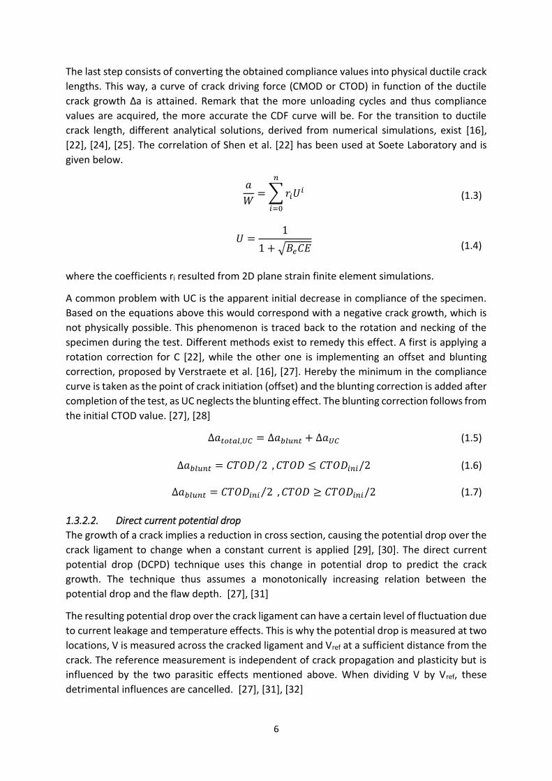
The last step consists of converting the obtained compliance values into physical ductile crack
lengths. This way, a curve of crack driving force (CMOD or CTOD) in function of the ductile
crack growth Δa is attained. Remark that the more unloading cycles and thus compliance
values are acquired, the more accurate the CDF curve will be. For the transition to ductile
crack length, different analytical solutions, derived from numerical simulations, exist [16],
[22], [24], [25]. The correlation of Shen et al. [22] has been used at Soete Laboratory and is
given below.
𝑎
𝑊= ∑ 𝑟𝑖𝑈
𝑖
𝑛
𝑖=0
(1.3)
𝑈 =
1
1 + √𝐵𝑒𝐶𝐸
(1.4)
where the coefficients ri resulted from 2D plane strain finite element simulations.
A common problem with UC is the apparent initial decrease in compliance of the specimen.
Based on the equations above this would correspond with a negative crack growth, which is
not physically possible. This phenomenon is traced back to the rotation and necking of the
specimen during the test. Different methods exist to remedy this effect. A first is applying a
rotation correction for C [22], while the other one is implementing an offset and blunting
correction, proposed by Verstraete et al. [16], [27]. Hereby the minimum in the compliance
curve is taken as the point of crack initiation (offset) and the blunting correction is added after
completion of the test, as UC neglects the blunting effect. The blunting correction follows from
the initial CTOD value. [27], [28]
∆𝑎𝑡𝑜𝑡𝑎𝑙,𝑈𝐶 = ∆𝑎𝑏𝑙𝑢𝑛𝑡 + ∆𝑎𝑈𝐶
(1.5)
∆𝑎𝑏𝑙𝑢𝑛𝑡 = 𝐶𝑇𝑂𝐷 2⁄ , 𝐶𝑇𝑂𝐷 ≤ 𝐶𝑇𝑂𝐷𝑖𝑛𝑖/2
(1.6)
∆𝑎𝑏𝑙𝑢𝑛𝑡 = 𝐶𝑇𝑂𝐷𝑖𝑛𝑖 2⁄ , 𝐶𝑇𝑂𝐷 ≥ 𝐶𝑇𝑂𝐷𝑖𝑛𝑖/2
(1.7)
1.3.2.2. Direct current potential drop
The growth of a crack implies a reduction in cross section, causing the potential drop over the
crack ligament to change when a constant current is applied [29], [30]. The direct current
potential drop (DCPD) technique uses this change in potential drop to predict the crack
growth. The technique thus assumes a monotonically increasing relation between the
potential drop and the flaw depth. [27], [31]
The resulting potential drop over the crack ligament can have a certain level of fluctuation due
to current leakage and temperature effects. This is why the potential drop is measured at two
locations, V is measured across the cracked ligament and Vref at a sufficient distance from the
crack. The reference measurement is independent of crack propagation and plasticity but is
influenced by the two parasitic effects mentioned above. When dividing V by Vref, these
detrimental influences are cancelled. [27], [31], [32]

7
The plasticity at the crack tip additionally influences the potential drop. In literature a three
phase evolution is described for V/Vref as a function of CMOD, see figure 1.4.
Figure 1.4: Typical evolution of normalized potential drop versus CMOD [31]
Firstly, a strong increase in potential drop is observed (phase 1) due to the separation of the
crack surfaces which may be electrically connected by debris. In the second phase, the linear
increase is ascribed to the plasticity around the blunting crack tip. This trend is represented
by the blunting line. The third phase, ultimately, describes a strong increase in potential drop.
This is attributed to as the actual crack tip propagation and thus the difference between the
graph and the blunting line is the actual potential drop that is related to ductile crack growth.
Just as with the UC method, the measured values have to be related to a physical crack length.
Johnson [33] proposed an analytical solution for compact cracked tension (CCT) specimens,
but this solution can also be applied to SENT and SENB specimens. The potential drop for the
actual crack depth 𝑉(𝑎) is normalized to the potential drop measured for the initial crack
depth 𝑉(𝑎0). [27], [31]
𝑉(𝑎)
𝑉(𝑎0)=
𝑐𝑜𝑠ℎ−1(cosh (9𝜋 4𝑊)⁄cos(𝜋𝑎 2𝑊⁄ )
)
𝑐𝑜𝑠ℎ−1(cosh (9𝜋 4𝑊)⁄cos(𝜋𝑎0 2𝑊⁄ )
)
(1.8)
Because this method does not take the crack propagation due to blunting into account, this
effect should be added at the end of the test in the same way as for UC. [27], [31]
∆𝑎𝑡𝑜𝑡𝑎𝑙,𝐷𝐶𝑃𝐷 = ∆𝑎𝑏𝑙𝑢𝑛𝑡 + ∆𝑎 𝐷𝐶𝑃𝐷
(1.9)
1.3.2.3. 3D Digital image correlation
Digital image correlation (DIC) is a technique that enables full field deformation and strain
measurements. This allows CTOD identification, for instance using the δ5 concept, see section
1.2.1. The 3D DIC technique uses a stereovision system consisting of two synchronized
cameras which make photos at predefined time steps. The specimen is painted white, with a
random black speckle pattern applied on top of it. The optimal speckle size depends on the
resolution and window covered by the cameras and is around 3x3 pixels. The displacement of
the speckles in the x, y and z direction are tracked by the DIC software by correlating the
photos made based on the movement of the speckles. This way, 3D displacements and 2D
strains in the plane of the specimen surface are obtained. [3], [6], [34], [35]

8
Tracking δ5 with DIC is beneficial when use of clip gauges is impractical [6], [14], [36].
Verstraete et al. [6] showed that both the methods using clip gauges and the one using DIC
give good correspondence, the δ5 value being somewhat higher than the CTOD90 value for
increasing initial crack ratio.
1.4. Weld strength heterogeneity Fusion welding of two metallic materials is achieved by melting base material and filler
material. High heat fluxes are applied in order to reach the melting phase, giving rise to large
temperature gradients in the material. Briefly, different regions in the weld have various
thermal histories leading to different microstructures, which constitutes the heterogeneous
nature of the weld. Out of a strength perspective various microstructures behave differently
towards crack propagation and plastic deformation in the vicinity of a crack tip. [37]
1.4.1. Characterization The strength heterogeneity of a weld can be characterised in different ways. The distribution
of different microstructures is mostly done based on hardness tests or miniature tensile
testing. Depending on the desired accuracy, available time and cost one can opt for one of
these two.
Hardness is closely related to the ultimate tensile strength (UTS) of a specimen, but not
necessarily to strain hardening Y/T and strain hardening exponent n. Used relations in linking
these properties are merely indicative to what could be representative properties. [38]
Miniature tensile tests have been used by Mohr and Koçak et al. and Hertelé et al. [39]–[41].
Compared to hardness tests, tensile tests provide insights in strain hardening as complete
stress to strain curves are obtained for every specimen. This enables comparison of full range
tensile properties of base metal, heat affected zones and weld metal. The sample orientation
can be taken through thickness or longitudinal with the weld. Longitudinal oriented specimens
sample over different cross sections of the weld but cover a certain microstructure
distribution. Through-thickness specimens cover more than one weld pass and they incline to
fail at the weakest microstructure.
1.4.2. Weld homogenization Traditionally weld assessment procedures involve many simplifications in order to conduct
the analysis. Taking into account the various microstructures present in weld flaw assessment
procedures is very challenging.
Consequently, even to date, most assessment practices still use strong approximations. The
most extreme simplification is assuming the weld metal properties to be equal to the base
metal properties, e.g. ref. [2]. Hereby, the reality of a weld being mismatched is ignored. Also
note that this approach is non-conservative for undermatched welds. Increasing the
complexity of the model is achieved by assuming the weld to be a strip of homogeneous
microstructure and properties but being dissimilar to those of the base metal, while ignoring
effects of heat affected zones and fusion interfaces. Wang et al. [42] reported that weld
assessment methods R6, SINTAP, FITNET FFS use this kind of modelling. This approach may
result in non-conservative or severely conservative results. Exceptionally some models

9
represent the weld as being composed by two zones of different properties. Kozak et al. [43]
and Predan et al. [44] presumed a zone of undermatched and one of overmatched weld metal
with the crack propagating perpendicular to the mismatch interface.
However, rather than a discrete number, a continuous variation of microstructures is present
in a weld and their distribution in space can vary strongly. Recently, a model has been
proposed by Hertelé et al. [38] which handles the wide spread of properties in the weld in the
prediction of the crack driving force. This model is summarized below.
The approach aims at downsizing a complex weld with different microstructures and non-
straight fusion lines into an equivalent homogeneous weld with vertical fusion lines, a so called
“idealised weld”. It starts from the idea that crack driving force is influenced by “global”
mismatch (as opposed to fracture toughness, which depends on “local” mismatch) [20].
The homogenisation uses results of slip line theory (see chapter 3). Concretely, average
strength properties are evaluated along an assumed slip line trajectory 𝑂𝐹:
𝑀𝑒𝑞 =∫ 𝑀(𝑠)𝑑𝑠
𝑂𝐹
‖𝑂𝐹‖
(1.10)
Where 𝑀(𝑠) = 𝜎𝑦𝑤(𝑠)/𝜎𝑦𝑏 represents the local mismatch factor, expressing the ratio of the
local yield strength of the material to the assumedly constant yield strength of the base
material. It should be stressed that the slip lines in this method are currently assumed under
an angle of 45° with the crack direction. This value results from the slip line theory (see chapter
3). The end point F of the slip line is taken on the fusion line. Due to the different
microstructures of the HAZ (HAZ softening or HAZ hardening), its effect is thus included in the
analysis.
Thus the equivalent weld has a homogeneous structure characterized with a strength
mismatch 𝑀𝑒𝑞, and straight fusion lines having a half width 𝐻𝑒𝑞 equal to the horizontal
projection of 𝑂𝐹, see figure 1.5.
Figure 1.5: Homogenization of a symmetric weld [38]
Furthermore, numerical investigations have indicated that the theory is well complying for
non-symmetrical crack locations, as is the case for e.g. HAZ cracks and that it is more suitable
to take the HAZ/ base metal boundary as end point for the slip line. A modification to the
definition of 𝑀𝑒𝑞 is than suggested. Here two points 𝐹𝑐 and 𝐹𝑅 are defined, one at each side
of the notch, giving rise to a 𝐻𝑒𝑞,𝐿 and 𝐻𝑒𝑞,𝑅, see figure 1.6. Here the strength is leveled out
over the whole width instead of one half for a symmetric weld.

10
𝑀𝑒𝑞 =∫ 𝑀(𝑠)𝑑𝑠
𝐹𝐿𝑂𝐹𝑅
‖𝑂𝐹𝐿‖ + ‖𝑂𝐹𝑅‖
(1.11)
Figure 1.6: Homogenization of a non-symmetric weld [38]
Figures 1.5 and 1.6 show slip lines starting at the crack tip and propagating under 45° [45],
[46]. When the real slip lines are deviating from the predicted path, the equivalent weld will
incorrectly represent the real weld, leading to a false weld flaw assessment. It is therefore of
paramount importance to have approximate slip line estimations, as this homogenisation
method loses accuracy when this is not the case (see chapter 3). However, slip line theory
assumes homogeneous material properties. Clearly, this does not comply with the
heterogeneous nature of a weld. This research will aim at investigating the relation between
the weld heterogeneity and the slip line evolution.
1.5. Conclusions Weld heterogeneity is present in each weld and is of major importance with respect to the
fracture assessment of a weld. Nevertheless today’s ECA methods do not take its complexity
into account.
One theory for transforming a heterogeneous weld into an equivalent homogeneous weld has
been recently developed at Soete Laboratory. This theory requires knowledge of the slip line
trajectory originating from the crack tip.

11
Chapter 2 Motivation for further research
2.1. Problem statement The previous chapter shows that the behaviour of the slip lines in complex heterogeneous
welds goes with strong simplifications and assumptions. In order to get a better understanding
and eventually being able to predict slip line behaviour, its interaction with complex weld
heterogeneity deserves attention. In light hereof, the following research objectives will be
tackled in this work.
Significant research is found in literature concerning the theory of plasticity, resulting
in theoretical slip line patterns for various configurations. Hereto theoretical solutions
for SENT specimens will be evaluated.
A procedure visualizing the path through the specimen is beneficial in improving
Ghent’s University weld homogenization model. For maximum potential in performing
future work, this should be possible for both experimental as numerical SENT
specimens.
2.2. Research approach A better understanding of the slip line evolution would contribute to the reduction of
conservatism in ECA. Lowering the conservatism level will result in less unnecessary reworking
of welds.
This work focuses on SENT specimens, resembling a low-constraint defective weld. With the
initial crack being milled over the entire specimen width, SENT specimens are perfectly suited
for weld characterization and visualization during testing.
The research approach consists out of the following steps.
1. Establishing algorithms for the extraction of slip line data from SENT experiments and
simulations. Both experiments and simulations use a different software and data
handling approach. The goal is to develop a procedure of extracting the data that
concerns the slip lines and to write software to process the data.
2. The algorithms in step one are validated by performing tension tests on ‘dummy’
specimens. These specimens consist out of plain base metal without a weld.
Theoretical solutions for the slip line pattern in such specimens are known, and as such

12
the accuracy of the algorithms can be demonstrated and the correspondence between
experimental and numerical analysis can be evaluated.
3. The last step in this work is to apply the developed algorithms. For the experimental
branch, welded specimens are tested and their slip line behaviour is studied. Based on
the results of the first experiments on the ‘dummy’ specimens of step two, a numerical
study focuses on examining the influence of various boundary conditions and material
properties on the slip lines for pure base material, i.e. not containing a weld.
With this work the basis for future research at Soete laboratory in the domain of slip line
behaviour will be provided and the specific areas that need further attention will be
highlighted.

13
Chapter 3 Slip line analysis 3.1. Introduction The research done in this thesis focuses on the slip line patterns that are observed in SENT-
specimens. The principle of slip lines will be outlined in this chapter, first by providing
theoretical insights into the subject (section 3.2). To be able to study slip line behaviour in
SENT specimens, they have to be visualized. Algorithms have been developed to extract the
slip line information from test or simulation data, see section 3.3. The study of the path of slip
lines is tracked with the help of slip line angles. These angles result from regression analysis,
as is explained in section 3.4. Next, section 3.5 describes the numerical implementation of the
algorithm and the regression analysis. Finally, the chapter is concluded with a verification of
the results obtained from the experimental and numerical approach by performing two
experimental SENT tests on plain base metal and simulating the same tests in the finite
element software ABAQUS®.
3.2. Theoretical background
3.2.1. Slip line field theory Slip line field theory (SLF) is an analytical technique of describing the lines of plasticity in a
rigid-perfectly plastic body in plane strain. The significance of this theory decreases, as it is
applicable for a limited set of simplified cases, while FEA on the other hand can be used as a
robust alternative to investigate more complex cases. Nevertheless a basic understanding of
slip line theory is vital to properly interpret the data. Hill [47] provides a basic overview of slip
line theory, discussed below.
Basically the following assumptions [48] are made in this analysis:
1. An rigid – perfectly plastic solid, i.e. an infinite yield Young’s modulus and perfectly
plastic after yielding, i.e. no work hardening
2. Plane strain deformation in the (x,y) plane, i.e. 𝜎2 =1
2(𝜎𝑥 + 𝜎𝑦) and 𝜀2 = 0
3. Quasi-static loading
4. No temperature changes and no body forces
5. Isotropic material
6. No Bauschinger effect
Consequently the theory is ignoring effects of strain-rate, strain hardening and large
deformations.

14
The equilibrium equations for plane strain plastic flow are
𝜕𝜎𝑥
𝜕𝑥+
𝜕𝜏𝑥𝑦
𝜕𝑦= 0
(3.1)
𝜕𝜏𝑥𝑦
𝜕𝑥+
𝜕𝜎𝑦
𝜕𝑦= 0
(3.2)
The critical shear stress, denoted by k, is a constant value when yielding is not influenced by
the hydrostatic pressure and no work hardening is present. According to the yield criterion
used it can be YS/2 with Tresca’s criterion or YS/√3 with von Mises’ criterion. The yield
criterion is then expressed as
1
4(𝜎𝑥 − 𝜎𝑦)
2+ 𝜏𝑥𝑦
2 = 𝑘²
(3.3)
Thus three stress equations with three unknowns 𝜎𝑥, 𝜎𝑦 and 𝜏𝑥𝑦 are obtained. Although as
mentioned by Johnson et al. [49], the stress boundary conditions are generally not adequate
to attain a definite solution for the stresses. Nevertheless the set of equations is satisfied by
following proposed solution
𝜎𝑥 = −𝑝 − 𝑘 sin 2𝜑
(3.4)
𝜎𝑦 = −𝑝 + 𝑘 sin 2𝜑
(3.5)
𝜏𝑥𝑦 = 𝑘 cos 2𝜑
(3.6)
𝜎𝑧 = −𝑝
(3.7)
With −𝑝 the hydrostatic part of the stress tensor. Obviously, this solution must satisfy the
equilibrium equations. When substituted, a hyperbolic set of equations is obtained for which
a solution of characteristics exists. From this same theory, it follows that the families of
characteristics, also called slip lines, are perpendicular to each other. By convention, the α-
family is given the direction 𝜑 with respect to the (x,y) coordinate system and the β-family the
direction 𝜑 + 𝜋/2.
As shown in figure 3.1, the characteristics correspond with the directions of maximal shear
stress. The solution can also be visualized in a Mohr circle (figure 3.2).
Satisfying the equilibrium equations results in the characteristics, also referred to as the
Hencky relations
𝑝 + 2𝑘𝜑 = 𝑐𝑜𝑛𝑠𝑡𝑎𝑛𝑡 𝑜𝑛 𝑎𝑛 𝛼 − 𝑙𝑖𝑛𝑒
(3.8)
𝑝 − 2𝑘𝜑 = 𝑐𝑜𝑛𝑠𝑡𝑎𝑛𝑡 𝑜𝑛 𝑎𝑛 𝛽 − 𝑙𝑖𝑛𝑒
(3.9)

15
Figure 3.1: Stresses on an infinitesimal element bounded by slip lines [50]
These characteristics can be seen as the equivalence of the equilibrium equations in case of
plane strain plastic flow. So these equations represent the equilibrium relations, but the
constants can vary between the slip lines. The hydrostatic stress can be calculated at every
point of the slip line. Based on the Hencky equations it is found that for straight slip lines (𝜑 =
constant) the hydrostatic stress remains constant. [47], [49]
Figure 3.2: Stresses and characteristics in plane strain with its corresponding Mohr circle [49]
A similar argumentation can be conducted for the velocity components. The plane strain
assumption results in a zero z-velocity, and non-zero x-and y-velocities 𝑣𝑥 and 𝑣𝑦.
Starting with the continuity and isotropy equations, a set of two velocity characteristic families
can be deduced, having the same directions as the stress characteristics. From this, the
following set of equations is derived, with 𝑢 the velocity in the 𝛼 direction and 𝑣 in the 𝛽
direction.
𝑑𝑢 − 𝑣 𝑑𝜑 = 0 𝑜𝑛 𝑎𝑛 𝛼 − 𝑙𝑖𝑛𝑒
(3.10)
𝑑𝑣 + 𝑢 𝑑𝜑 = 0 𝑜𝑛 𝑎 𝛽 − 𝑙𝑖𝑛𝑒 (3.11)

16
This set of equations is also referred to as the Geiringer equations.
As already mentioned, the characteristics of stresses and velocities coincide, meaning that the
direction of maximum shear stress and shear strain-rate coincide.
Generally, both stress and velocity boundary conditions are needed to obtain a solution for
the slip line field. A short description of important stress boundary conditions is given in the
next section. [49]
Please note that the derivations above start from plane strain conditions. However, slip line
theory has been also determined in case of plane stress conditions with the same method of
characteristics. The plane stress discussion is more involved resulting in more complex
equations. For a more detailed discussion, the reader is referred to [47], [51]. Nevertheless,
as plane stress condition are important in this work, section 3.2.2 will give the solution for
plane stress boundary conditions too. All other remaining subsections of section 3.2 will start
from the classical slip line theory in plane strain.
3.2.2. Boundary condition: stress free surface
Plane strain:
In case of a stress-free surface, no normal and shear stress component can exist at the surface.
This means that the normal and tangential direction at the free surface are directions of
principle stress. As slip-lines are lines of maximal shear stress in the material, they
consequently intersect the free surface at an angle of ±45°. Yielding will then occur for a
tension (or compressive stress) of 2𝑘, resulting in an shear stress of 𝑘. [45], [49], [51]
Plane stress:
If the specimen is loaded in plane stress, slip lines will make an angle of ±54.44° with the stress
free specimen surface. [51]
Remark that both stress states are important in the study of slip lines in SENT specimens.
When considering sections inside the material that are removed sufficiently from the
specimen outer surface, e.g. the mid-section, plane strain conditions can be assumed. On the
outer surfaces of the specimen, plane stress conditions occur. Another effect that will be
important is the deformation of the specimen surface opposing the surface of the original
crack. Consequently, the angle of the slip lines at that surface will have to change accordingly
in order to fulfill the boundary condition.
3.2.3. Predicted pattern for SENT configuration In reality however, a combination of two patterns can intervene. Slip lines start under 45° at
the free surface and crack tip according to a plate in tension. When the notch grows deeper,
the constraint level changes and the loading condition in the uncracked ligament more
approaches that of a specimen in bending. The slip lines will therefore deviate according to
the solution in bending and finally reach the free surface at 45° as is demanded by the
boundary condition, see figure 3.3. [16], [47], [49], [50], [52]
The different slip line behavior in bending (figure 3.3) originates from the stress field evolution
in the uncracked ligament of the specimen. This section experiences a linear stress distribution
corresponding with that of a beam in bending. The sign of the stresses changes at the mid-

17
section of the ligament. Assuming the bending moment positive in figure 3.3, the upper half
of the uncracked ligament experiences tensile stresses, while the lower half is compressed.
The sign change causes the slip lines to turn inwards and make the curvature as shown in
figure 3.3.
Figure 3.3: Slip lines for a plate in bending (SENB test) [52]
3.2.4. Extension of theory to material interfaces The theory given above is valid for homogeneous isotropic material, in which plasticity always
occur in the direction of maximum shear stress. Nonetheless, extensions have been developed
to predict the behaviour of slip lines along the boundary between two different materials.
From the fundamental analysis it follows that discontinuities in velocity, velocity gradient and
stress gradient can occur across such a material interface. Prager [53] described this
behaviour.
The equilibrium equations call for continuity in normal and shear stresses at both sides of the
slip lines (figure 3.4)
𝜎𝑛+ = 𝜎𝑛
−
(3.12)
𝜏+ = 𝜏−
(3.13)
Although the tangential stresses parallel to the curves can differ from each other
𝜎𝑡+ ≠ 𝜎𝑡
−
(3.14)
The difference in tangential stress across the slip line is bounded by the need of plasticity at
both sides. [45], [47]
Next to the stresses, the displacement continuity across the interface has to be considered.
Expressed along the directions of principal stresses, the continuity condition is [45]
𝑣1+ = 𝑣1
− ; 𝑣2+ = 𝑣2
−
(3.15)
Expressed along the slip lines, the Geiringer relations give a sufficient condition for the
displacement continuity of slip lines across an interface [45]
𝜑𝐵+ − 𝜑𝐴
+ = 𝜑𝐵− − 𝜑𝐴
−
(3.16)

18
Figure 3.4: Slip lines at a material interface [45]
3.2.5. Analytical versus experimental/numerical observations Attempts have been undertaken to validate the relevance of slip line theory to the assessment
of cracked welds.
Hao et al. [45] and Kim et al. [54] (GKSS) published an overview of slip-line fields that can be
expected in centre cracked mismatched welds for elastic-plastic materials in plane strain.
These fields were than used to derive analytical solutions of limit load and constraint for each
configuration. Validation was conducted through finite element analysis (FEA). The weld was
considered as homogeneous and having a strength mismatch with respect to the base metal
expressed by (𝜎𝑦𝑤 being the weld yield strength and 𝜎𝑦𝑏 the yield strength of the base metal)
𝑀 =
𝜎𝑦𝑤
𝜎𝑦𝑏.
(3.17)
Furthermore the heat affected zone was ignored and the fusion lines were considered vertical,
resulting in an “idealized” weld configuration.
Hao et al. [45] and Kim et al. [54] analyzed both under and overmatching welds and classified
the different patterns that were observed according to the geometry of the specimen and
crack length, see figure 3.6. The parameter used is representing the ratio of the rest ligament
to the specimen height 𝜓 = (𝑊 − 𝑎) 𝐻⁄ .
Undermatched welds
For welds of higher width ((𝑊 − 𝑎) 𝐻⁄ < 1) the slip lines make an angle of 45° with the axis
of the original crack. In case of slender welds ((𝑊 − 𝑎) 𝐻⁄ > 1) cycloidic slip line patterns are
obtained, combined with a so called Prandtl field at the crack tip. A Prandtl field is a slip line
field surrounding a crack tip, see figure 3.5, under small-scale yielding (SSY) in homogeneous,
perfectly plastic materials. This field however requires high constraint conditions around the
crack tip. Such conditions are imposed when the crack tip is still surrounded by an elastic zone,
but may disappear otherwise. An example is the case of slim undermatched welded joints,
where the rigid base material hinders large plasticity around the crack tip and thus enforces
high constraints. In this case, the Prandtl field lasts and even grows under fully plastic

19
conditions. The Prandtl field at the crack field can then combine with the cycloid fields
explained before.
Figure 3.5: Prandtl field at a crack tip [52]
Although these patterns can be deducted analytically for homogeneous welds, they are
generally not observed in real tension tests and finite element simulations.
Kim et al. [54] simulated compact tension (CT) and single edge notched bending (SENB) tests
and observed two main distinct patterns occurring for undermatched welds. The zones of
plasticity are not showing the solutions listed before but are simple curve like regions that are
either confined to the weld metal (small M and small 𝜓), or penetrate into the base metal
(figure 3.6).
Figure 3.6: Plasticity patterns for over- and undermatched centre cracked welds [54]

20
Overmatched welds
Generally, welds are aimed to be overmatched. This is beneficial when overloaded, since
yielding will be distributed over the base metal instead of being concentrated merely in the
weld. Further slip line analysis in this work concentrates on these overmatched welds.
In case of low overmatching, the slip-line pattern is similar to the pattern for small
undermatching, i.e. slip lines penetrating into the base metal with lines under approximately
45° (figure 3.6).
Strong overmatching leads to failure of the base material and slip lines starting at the
intersection of the interface with the free edge (figure 3.6a).
To conclude this discussion, an alternative to slip line analysis should be mentioned. When
dealing with plastic behaviour, often lower- and upper-bounds are estimated. This approach
is stating a lower, being an underestimation and upper bound, being an overestimation for
the load that leads to a certain deformation. This theory is also referred to as limit analysis
[55]. The theory is more straightforward than slip line analysis and can lead to good
approximations. The upper bound results from the principle of a kinematically admissible
velocity field that complies with the internal strains and the displacements imposed at the
boundaries. The lower bound follows from a statically admissible stress field, which satisfies
the forces at the boundaries. So while the upper bound solution for loading corresponds with
a correct displacement field, the lower bound solution agrees with an admissible stress field.
[55], [56]
3.2.6. Equivalent plastic strain Paragraph 3.3 will make use of the maximum equivalent plastic strain throughout its analysis.
R. Hill described in his work “The Mathematical Theory of Plasticity” [47], the theoretical
derivation of equivalent plastic strain which is briefly recapitulated next.
If von Mises plasticity is assumed, equivalent (or von Mises) plastic strain 𝜀𝑒𝑞𝑝 , with ‘p’ referring
to plastic, should relate with equivalent (or von Mises) stress as true stress relates with true
plastic strain in a uniaxial tensile test. Therefore, the following definition is introduced:
𝜀𝑒𝑞
𝑝 = ∫ 𝜀�̇�𝑞𝑝 𝑑𝑡
𝑡
0
(3.108)
in which
𝜀�̇�𝑞𝑝
= √2
3𝜀�̇�𝑗
𝑝𝜀�̇�𝑗
𝑝
(3.19)
This equation can equivalently be expressed in terms of deviatoric strains 𝜀𝑖𝑗′ since 𝑑𝜀′𝑖𝑗
𝑝=
𝑑𝜀𝑖𝑗𝑝 . This is true since conservation of volume implies that 𝑑𝜀𝑖𝑖
𝑝 = 0.
If loading is proportional, the integration reduces to

21
𝜀𝑒𝑞𝑝
= √2
3𝜀𝑖𝑗
𝑝𝜀𝑖𝑗
𝑝
(3.20)
If the coordinate system is oriented along the directions of the principal plastic strains
𝜀1𝑝, 𝜀2
𝑝, 𝜀3𝑝, this equation can be written as
𝜀𝑒𝑞𝑝 = √
2
3 ((𝜀1
𝑝)2
+ (𝜀2𝑝)
2+ (𝜀3
𝑝)2
)
(3.21)
The principle of conservation of volume implies that
𝑑𝜀1𝑝 + 𝑑𝜀2
𝑝 + 𝑑𝜀3𝑝 = 0 (3.22)
The assumption of proportional loading, reduces the latter to
𝜀1𝑝 + 𝜀2
𝑝 + 𝜀3𝑝 = 0 (3.23)
Given this, the equation for equivalent plastic strain Eq. 3.21 can be rewritten by substituting
𝜀3 by −𝜀1 − 𝜀2
𝜀𝑒𝑞
𝑝 =2
√3√((𝜀1
𝑝)2
+ (𝜀2𝑝)
2+ 𝜀1
𝑝𝜀2𝑝)
(3.24)
This equation is also recovered in reference [57]. In the same analogy, also a definition for
equivalent total strain 𝜀𝑒𝑞 can be defined:
𝜀𝑒𝑞 =
2
√3√((𝜀1)2 + (𝜀2)2 + 𝜀1𝜀2)
(3.115)
This will be used in section 3.4, as in the experimental analysis the output data does not allow
to make the distinction between total and plastic strain.
3.3. Algorithm to determine slip lines A slip line connects the points of maximum shear strain. Starting point in the determination
of the slip lines is the evaluation of all plastic strains in a specific section of the specimen. This
section can be an outer surface, but also an inner plane of the specimen (in case of
simulations). If the surface under investigation is designated as the XY-plane, the following
strains have to be known in that section: 𝜀𝑥𝑥, 𝜀𝑦𝑦, 𝜀𝑥𝑦. With these strains, the in-plane
principal strains 𝜀1 and 𝜀2 can be calculated as follows.
𝜀1 =𝜀𝑥𝑥 + 𝜀𝑦𝑦
2+ √(
𝜀𝑥𝑥 − 𝜀𝑦𝑦
2)
2
+ (𝜀𝑥𝑦
2)
2
(3.26)

22
𝜀2 =𝜀𝑥𝑥 + 𝜀𝑦𝑦
2− √(
𝜀𝑥𝑥 − 𝜀𝑦𝑦
2)
2
+ (𝜀𝑥𝑦
2)
2
(3.27)
To make the definition of the principal coordinate system unambiguous, 𝜀1 is chosen larger
than 𝜀2.
Once the principal strains in the specific section of interest are known, the slip lines can be
determined by defining a grid in the XY-plane as shown in figure 3.7.
Figure 3.7: SENT specimen with a grid defined
This grid is used for purpose of discretizing the data in the plane of interest. The grid divides
the X-axis into intervals with width ∆𝑥 and ∆𝑦 for the Y-axis (figure 3.8). Together with 𝑛𝑥
and 𝑛𝑦, which are the number of grid lines along the X-and Y-axis respectively, the region of
interest for slip line analysis can be covered with a grid.
Figure 3.8: Grid dimensions and syntax
Y
X
F
F
Side groove notch
grid
-4 -3 -2 -1 0 1 2 3 4-25
-20
-15
-10
-5
0
5
10
15
20
25

23
To determine the grid resolution, a convergence study of various grid meshes has been
performed. Table 3.1 gives the different options that have been verified by specifying the
number of points in the X- and Y-direction, together with their corresponding intervals,
expressed in coordinate units of the XY-coordinate system.
Table 3.1: Grid convergence study
𝑛𝑥 𝑛𝑦 ∆𝑥 ∆𝑦 Extraction
time (s)
20 80 0.5 0.375 0.5
30 120 0.33 0.25 1
40 160 0.25 0.188 1.5
50 200 0.2 0.15 2
Also, the resolution of the grid is depending on the area that covered by the grid. The values
that are given in table 3.1 are based on a grid of 10 units wide in the X-direction and 30 units
high in the Y-direction. These values have been found to cover the complete slip line area in
the experiments reported in chapter 4. Please note that depending on the size of the
specimens and the specimen material, the overall grid dimensions can differ from those used
in this study.
Clearly, the grid with the highest number of points has the highest accuracy but also the
highest data load. However, as Matlab® will be used for further data processing after
extraction, large amounts of data can be processed easily. The bottleneck in the grid choice
could be the data extraction from digital image correlation (DIC). The extraction procedure is
covered in detail in appendix A, however the following remarks can be made at this point.
The maximum number of points in the X or Y-direction that can be extracted with one
grid amounts to 200.
The time for the extraction of a grid from one DIC picture is shown in table 3.1
0.01 is the finest interval between adjacent grid points for data extraction in the DIC
post processing software VIC3D®
As table 3.1 shows, the extraction of the data is not an issue. With the highest grid resolution
and for instance a total number of 30 DIC pictures, the total time of extraction is only one
minute. As this time lapse is more than acceptable, the 50x200 grid will be used further on in
this work. As a coordinate unit in DIC corresponds with one physical millimeter, the 50x200
has a grid resolution that suffices for the slip line analysis.
Through the definition of the grid, the large number of data points in the plane of interest that
result from numerical analysis with VIC3D® or the finite element software ABAQUS® are
reduced into a predefined and manageable number of grid points. Furthermore, the grid is
deformable, meaning that it tracks the location of the intersection points during the
specimen’s deformation (figure 3.9).

24
Figure 3.9: Grid deforms during the test
In addition to the strains mentioned above, the displacement of each intersection point and
the crack tip displacement are needed for the analysis.
𝑈 is the X-displacement of a grid point
𝑉 is the Y-displacement of a grid point
𝑈𝑐 is the X-displacement of the crack tip
𝑉𝑐 is the Y-displacement of the crack tip
The next step in finding the slip lines is using the strains at each grid location to determine the
maximum equivalent plastic strain along each array of grid points parallel to the X-axis (figure
3.7). It is advised to determine the maximum along the grid lines parallel to the initial crack,
i.e. parallel to the X-axis, as in this way each line only intersects one slip line (one slip line exists
at each side of the crack). The other option (finding maxima along Y-grid lines) would make
the analysis more complex as in that case, “two maxima” have to be found along one grid line,
i.e. one for the upper and for the lower slip line.
At this point, 𝑛𝑦 maxima of equivalent plastic strain are determined, one for each grid line
parallel to the X-axis. Each maximum has its X and Y coordinates, i.e. 𝑥𝑚𝑎𝑥 and 𝑦𝑚𝑎𝑥, but the
location of the point has moved during testing as the specimen deforms. The X-and Y-
coordinate of the maxima have therefore to be corrected with its respective displacements
relative to the crack tip position. So the true X-and Y-coordinate of each maximum during
deformation is:
𝑥𝑚𝑎𝑥 = 𝑥 + 𝑈 − 𝑈𝑐
(3.28)
𝑦𝑚𝑎𝑥 = 𝑦 + 𝑉 − 𝑉𝑐
(3.29)
However, in the light of the homogenization theory that is developed at the laboratory with
the UGent model, the coordinates of the slip lines in the non-deformed state of the specimen
are to be determined. The UGent model starts from a specimen that keeps its initial non-
deformed shape. In this case, the coordinates of the slip lines are determined without using
the displacements 𝑈, 𝑉, 𝑈𝑐 and 𝑉𝑐:
𝑥𝑚𝑎𝑥 = 𝑥
(3.30)
𝑦𝑚𝑎𝑥 = 𝑦 (3.31)
-4 -3 -2 -1 0 1 2 3 4-25
-20
-15
-10
-5
0
5
10
15
20
25
-4 -3 -2 -1 0 1 2 3 4 5 6
-20
-15
-10
-5
0
5
10
15
20
25

25
Depending on the noise of the signal and the size of the defined grid, erroneous maxima may
be identified and data filtering is needed. Depending on whether data is originating from the
VIC3D® or the ABAQUS® software, different filtering algorithms have been applied to locate
the maxima belonging to each slip line (see section 3.5).
It may already be noted that during the first part of a test, no clear regions of large plastic
deformation are visible. The specimen is still in its elastic state. Determining maximum
equivalent strain will as such result in more of a random pattern and no clear slip lines will be
visible. Especially the analysis with VIC3D® suffers from this aspect. The procedure of slip line
behaviour analysis is therefore advised to be started when the slip lines are clearly visible and
their strains are dominant. Section 3.5 will give in depth information on this aspect.
3.4. Characterization of slip lines At this point, both slip lines originating from the notch tip can be drawn as two distinct curves
in the XY-plane. Starting from the X-and Y-coordinates of their discrete points, they can be
processed according to a regression analysis. From the regression lines their angle with the Y-
axis can be determined. To that end, different regression approaches have been investigated:
linear (section 3.4.1) and polynomial (section 3.4.2)
3.4.1. Linear regression Linear regression can be seen as the most easy and straightforward way of processing the slip
line data. Both the upper as lower slip line are processed separately, resulting in two
regression lines and two regression angles as shown in figure 3.10. For each dataset of the top
and bottom slip line, two coefficients 𝑎𝑖 and 𝑏𝑖 are determined (i = top or bottom)
𝑦𝑟𝑒𝑔 = 𝑎𝑖 ∙ 𝑥 + 𝑏𝑖 (3.32)
Figure 3.10: Slip lines with their linear regression line in a SENT specimen
Y
X
F
F
Lin. Reg.

26
3.4.2. Polynomial regression Polynomial regression fits an n-degree polynomial model to the slip line data. The degree n of
the polynomial is specified in advance and as such the coefficients 𝑎0, 𝑎1, …, 𝑎𝑛 of the
polynomial are determined.
𝑦 = 𝑎𝑛𝑥𝑛 + 𝑎𝑛−1𝑥𝑛−1+. . +𝑎1𝑥 + 𝑎0
(3.33)
n+1 points need to be specified for a regression line of the order n, as the equation contains
n+1 coefficients. For polynomial regression, each slip line has one regression line and the
number of angles that can be extracted from each slip line is dictated by the user. By specifying
the locations at which the derivative of the regression line should be evaluated, the slip line
angles result. For instance, the derivative can be evaluated for the same X-coordinates as the
slip line data points.
The concept is explained with help of figure 3.11 and table 3.2. In figure 3.11 polynomial
regression lines of a degree of four have been applied to the upper and lower slip line. As can
be observed, the regression lines nicely fit the data. Furthermore, the derivatives of the
regression lines are shown in the same figure. The derivatives give the slope of the regression
line and from those, the slip line angles can be determined. The derivatives are fairly constant
in the X-interval -1 to 4, as the slip lines are linear in that section. When the slip lines approach
the specimen surface, the slip line path will deviate from its linear trend.
Figure 3.11: Polynomial regression line
From the derivatives the slip line angles are calculated and reported in table 3.2. The slip lines
contain 15 data points, and for each X-value of the data points constituting the slip line, the
derivative is evaluated. Consequently, 15 slip line angles are obtained for each slip line. In
table 3.2 the slip line angles are listed starting at the notch of the specimen and proceeding
towards the specimen surface.
-4 -2 0 2-8
-6
-4
-2
0
2
4
6
8
specimen width [mm]
specim
en length
[m
m]
Slip line evolution during a SENT test
top slip line
bottom slip line
derivative top
derivative bottom
regression line
-5.3 -5.2 -5.1 -5 -4.9
-0.6
-0.5
-0.4
-0.3
-0.2
-0.1
0
0.1
0.2
0.3
specimen width [mm]
specim
en length
[m
m]
Slip line evolution during a SENT test
top slip line
bottom slip line
derivative top
derivative bottom
regression line

27
Table 3.2: Polynomial regression angles of the slip lines in figure 3.11
Slip Line Polynomial regression angle (°)
From the notch…
Top 50.0 47.3 45.3 44.1 43.5 43.5 43.9 44.8
bottom 46.3 46.4 47.2 47.7 48.2 48.3 48.4 48.5
…to the specimen surface
Top 46.2 48.1 50.5 53.5 60.6 69.7 85.2
Bottom 49.2 49.9 51.0 54.6 57.6 66.8 92.5
The angles lie between 45° to 50° for the linear section and increase towards the surface (see
numbers in bold). For the lower slip line the angle exceeds 90°, although this seems
contradictory when looking at figure 3.11. However when enlarging the graph around the
derivative in that section, it is observed that it the derivative is indeed negative at the start.
The reason for that is displayed on the left hand side of figure 3.12.
Figure 3.12: Polynomial regression with polynomial degree n = 4 (left), n = 6 (right)
The polynomial regression line that is fitted to the slip lines is decreasing strongly for X-values
lower than -6. Therefore the derivative will have a negative value at that point and the
resulting slip line angle is not accurate. This effect is strengthened when the polynomial
degree increases (see figure 3.12 and 3.13). The derivatives increase or decrease strongly at
the slip line end points and therefore the resulting angle at those outer points is biased as is
shown with the bold numbers in table 3.3.
-6 -4 -2 0 2-8
-6
-4
-2
0
2
4
6
8
specimen width [mm]
specim
en length
[m
m]
Slip line evolution during a SENT test
top slip line
bottom slip line
derivative top
derivative bottom
regression line top
regression line bottom
-6 -4 -2 0 2-8
-6
-4
-2
0
2
4
6
8
specimen width [mm]
specim
en length
[m
m]
Slip line evolution during a SENT test
top slip line
bottom slip line
derivative top
derivative bottom
regression line top
regression line bottom

28
Figure 3.13: Polynomial regression with polynomial degree n = 8 (left) and n = 10 (right)
If the polynomial degree is high, e.g. 10, the fit of the data even can be worse than with a
lower degree. The right hand side of figure 3.13 shows that the regression line clearly deviates
from the slip line trend in the region where the slip line meets the surface.
Table 3.3: Polynomial regression angle of the top slip line as function of polynomial degree
Degree Polynomial regression angle (°)
From the notch…
4 50.0 47.3 45.3 44.1 43.5 43.5 43.9 44.8
6 43.3 44.7 45.5 45.6 45.3 44.7 44.3 44.2
8 38.8 46.9 45.7 44.0 44.3 45.5 45.9 45.2
10 41.3 45.8 44.6 45.2 45.4 44.6 44.4 45.2
…to the specimen surface
4 46.2 48.1 50.5 53.5 60.6 69.7 85.2
6 44.8 46.3 48.9 52.8 64.1 75.7 61.8
8 44.1 44.2 47.2 53.9 69.9 56.7 156.2
10 45.9 45.3 45.1 49.7 85.5 30.9 176.9
It can be concluded that polynomial regression can be a powerful tool to observe the change
in slip line angle. By varying the degree of the polynomial regression line, a widespread of slip
line shapes can be described. However, the success of this technique is closely related to that
polynomial degree and the exact value of the latter is test specific. A too low or too high
degree results in a poor fit of the data, but also when the fit seems to be good at first sight,
the derivative of the regression line can vary strongly at the end points of the slip line. As the
slip line angle is calculated from the derivative this can lead to erroneous results.
-6 -4 -2 0 2-8
-6
-4
-2
0
2
4
6
8
specimen width [mm]
specim
en length
[m
m]
Slip line evolution during a SENT test
top slip line
bottom slip line
derivative top
derivative bottom
regression line top
regression line bottom
-6 -4 -2 0 2-8
-6
-4
-2
0
2
4
6
8
specimen width [mm]
specim
en length
[m
m]
Slip line evolution during a SENT test
top slip line
bottom slip line
derivative top
derivative bottom
regression line top
regression line bottom

29
Hereto, an alternative is proposed regarding the determination of the slip line angles from the
polynomial regression line. Instead of calculating the slip line angle from the derivative of the
polynomial regression line, piecewise linear regression can be applied. Hereto, calculate the
slip line angle from the linear slope between two consecutive points of the polynomial
regression line, e.g. again evaluated at the X-values of the slip line points:
𝑠𝑙𝑜𝑝𝑒 =
𝑦𝑟𝑒𝑔,𝑖+1 − 𝑦𝑟𝑒𝑔,𝑖
𝑥𝑟𝑒𝑔,𝑖+1 − 𝑥𝑟𝑒𝑔,𝑖 (3.34)
With this technique linear regression is applied on two consecutive points of the polynomial
regression line. The angles obtained from this method are much more robust.
3.5. Numerical implementation The algorithm elaborated in section 3.3 has been implemented both for experimental work
with DIC analysis, as for FEA simulations. This section describes how the data is manipulated
for both branches, starting in the first section with data originating from VIC3D® (DIC
software), while the second section repeats this for data obtained with ABAQUS® (FEA
software).
3.5.1. Experimental This section will give a short introduction into the algorithm for slip line determination starting
from the DIC analysis of an SENT test. The procedure is described generally and for an in depth
elucidation of the used code the reader is referred to appendix A. The DIC data is processed
in the VIC3D® software according to the following consecutive steps.
1. Calibrate the system
2. Define a region of interest and start the analysis
3. Let the software calculate the strains in the defined region
4. Extract the displacement and strain data according to a predefined grid (figure 3.7)
Steps one, two and three are straightforward and extensively explained in the VIC3D® manual.
Step four is highlighted in appendix A and this section will focus on the Matlab code® that uses
the extracted grid data, i.e. subsequent to step four. The coding has been continuously
improved during the year through three major iterations, towards a more efficient and
compact code.
3.5.1.1. Matlab® code
The Matlab® code consists of two scripts.
1. Script one, determineSlip.m, calculates the location of the maximum equivalent total
strains on each horizontal grid line for the grid data that are provided and returns script
two with the X and Y coordinate of these maxima (section 3.3).
2. The second script, dataProcessing.m, handles the output of the first script and filters
out the slip line trajectories. Regression analysis is performed on the slip lines and
various slip line manipulation techniques can be activated (section 3.4).

30
Script determineSlip.m: Determining the maximum equivalent total strains
Six input parameters are provided to this Matlab® script while the script returns the X and Y
coordinates of the slip lines, as shown in table 3.4.
Table 3.4: Input and output parameters of determineSlipcsv.m
Input parameters Description
xPoints Grid dimension in X-direction
yPoints Grid dimension in Y-direction
s Photo number of the DIC analysis
𝑈𝑐 Crack displacement in X-direction
𝑉𝑐 Crack displacement in Y-direction
Deformed Determine slip line in deformed coordinates
Output parameters Description
xCo List of X-coordinates along the slip line
yCo List of Y-coordinates along the slip line
The script starts by loading the data from the separate .csv files made by the extract node data
command in VIC3D®. For each DIC image a separate .csv file is generated, as explained in
appendix A. The possibility of writing all data to one script exists, but results in a chaotic and
large data file that is difficult to interpret. With one single file for each photo, a clear and
clarifying structure is obtained as highlighted in table 3.5. Every parameter is saved in a column
matrix.
Table 3.5: scheme .csv file
X [mm] Y [mm] U [mm] V [mm] 𝜀1 𝜀2 𝜀𝑣𝑜𝑛𝑀𝑖𝑠𝑒𝑠
-4.5 -5.5 … … … … … -4.0 -5.5 … … … … …
⋮ ⋮ 4.5 -5.5 … … … … …
-4.5 -4.5 … … … … … ⋮ ⋮
4.5 -4.5 … … … … …
⋮ ⋮
-4.5 5.5 … … … … … ⋮ ⋮
4.5 5.5 … … … … …
Table 3.5 shows the structure of the csv file if for example the grid is defined by X varying from
-4.5 to 4.5 in steps of 0.5 while Y varies from -5.5 to 5.5 in steps of 1. Each horizontal grid line
is written sequentially, starting with the lowest Y-values. The code recognizes the transitions
between the horizontal grid lines and saves the corresponding indices for the parameter
column matrices.

31
As at this point each horizontal grid line is demarcated, the maximum equivalent total strain
can be determined. Table 3.5 indicates that 𝜀𝑣𝑜𝑛𝑀𝑖𝑠𝑒𝑠 has initially been extracted from VIC3D®
and used as the equivalent total strain. However, a definition of that strain is not found in the
manual. Communication with the support team of Correlated Solutions Inc. (developers of
VIC3D® software) revealed that 𝜀𝑣𝑜𝑛𝑀𝑖𝑠𝑒𝑠 is defined as
𝜀𝑣𝑜𝑛𝑀𝑖𝑠𝑒𝑠 = √𝜀1
2 + 𝜀22 − 𝜀1𝜀2
(3.35)
The support team explained that this definition has been chosen in analogy with the equation
for von Mises stress in plane stress conditions:
𝜎𝑣𝑜𝑛𝑀𝑖𝑠𝑒𝑠 = √𝜎1
2 + 𝜎22 − 𝜎1𝜎2
(3.36)
This equation does not correspond with the concepts of equivalent plastic strain assuming
conservation of volume and proportional loading, resulting in Eq. 3.24.
To compare results originating from VIC3D® with those of ABAQUS®, as is discussed in the next
section, the predefined function of 𝜀𝑣𝑜𝑛𝑀𝑖𝑠𝑒𝑠 is therefore not used. Instead both in-plane
principal strains 𝜀1 and 𝜀2 are extracted and combined according to Eq. 3.24. Hereby it is
assumed that the linear-elastic component of strains included in the VIC3D® principle strains
is negligible with respect to the plastic component, as large plastic deformations are studied.
Once the index of maximum total strain is determined for each horizontal grid line, the
corresponding coordinates of that location have to be supplied to the second script. The
specimen will plastically deform during the test on the tension rig, which leads to two ways in
which the slip line coordinates can be acquired as explained in section 3.3, i.e. in the deformed
and non-deformed state.
The deformed state refers to a grid that deforms with the specimen. This means that to the X
and Y coordinates, the specific displacements 𝑈 and 𝑉, as the crack displacement 𝑈𝑐 and 𝑉𝑐
have to be added, according to Eqs. 3.28 and 3.29. On the other hand, for the non-deformed
state, the displacements are not used as the grid is assumed rigid, see Eqs. 3.30 and 3.31.
Script dataProcessing.m: Filter the slip lines and apply regression analysis
The coordinates of the locations of maximum equivalent total strain received from the first
script can contain a lot of noise, see figure 3.14. This noise is especially apparent for the initial
stage of the test, in which no clear slip lines are present yet (see figure 3.14 left). From a
certain point on, the onset of the slip lines can be observed. As the test proceeds, the slip lines
will become more dominant and the noise level will decrease in general. However, even when
the test has proceeded significantly, there may still be points included in the dataset that do
either not belong to the slip lines or belong to a secondary path of plasticity (see figure 3.14
right). This second path can be either due to the weld heterogeneity, but also due to other
influences as e.g. clip gauge knives that are positioned too close to the surface (see chapter 4
for more details). Figure 3.14 (right) shows a disadvantage of the method of selecting one
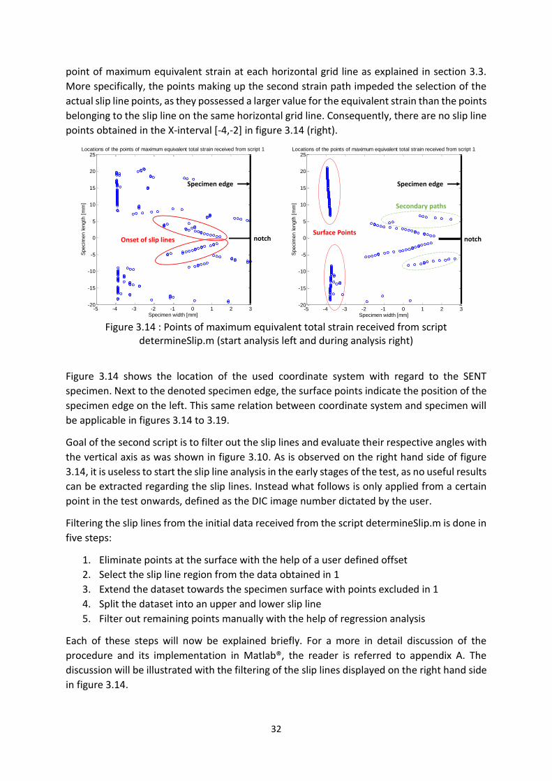
32
point of maximum equivalent strain at each horizontal grid line as explained in section 3.3.
More specifically, the points making up the second strain path impeded the selection of the
actual slip line points, as they possessed a larger value for the equivalent strain than the points
belonging to the slip line on the same horizontal grid line. Consequently, there are no slip line
points obtained in the X-interval [-4,-2] in figure 3.14 (right).
Figure 3.14 : Points of maximum equivalent total strain received from script
determineSlip.m (start analysis left and during analysis right)
Figure 3.14 shows the location of the used coordinate system with regard to the SENT
specimen. Next to the denoted specimen edge, the surface points indicate the position of the
specimen edge on the left. This same relation between coordinate system and specimen will
be applicable in figures 3.14 to 3.19.
Goal of the second script is to filter out the slip lines and evaluate their respective angles with
the vertical axis as was shown in figure 3.10. As is observed on the right hand side of figure
3.14, it is useless to start the slip line analysis in the early stages of the test, as no useful results
can be extracted regarding the slip lines. Instead what follows is only applied from a certain
point in the test onwards, defined as the DIC image number dictated by the user.
Filtering the slip lines from the initial data received from the script determineSlip.m is done in
five steps:
1. Eliminate points at the surface with the help of a user defined offset
2. Select the slip line region from the data obtained in 1
3. Extend the dataset towards the specimen surface with points excluded in 1
4. Split the dataset into an upper and lower slip line
5. Filter out remaining points manually with the help of regression analysis
Each of these steps will now be explained briefly. For a more in detail discussion of the
procedure and its implementation in Matlab®, the reader is referred to appendix A. The
discussion will be illustrated with the filtering of the slip lines displayed on the right hand side
in figure 3.14.
-5 -4 -3 -2 -1 0 1 2 3-20
-15
-10
-5
0
5
10
15
20
25Locations of the points of maximum equivalent total strain received from script 1
Specimen width [mm]
Specim
en length
[m
m]
Onset of slip lines
Specimen edge
notch
-5 -4 -3 -2 -1 0 1 2 3-20
-15
-10
-5
0
5
10
15
20
25Locations of the points of maximum equivalent total strain received from script 1
Specimen width [mm]
Specim
en length
[m
m]
Surface Points
Secondary paths
Specimen edge
notch

33
In the first step, the data points visualized in figure 3.14 are split according to their X-
coordinates. The user defines an offset with respect to the specimen surface and all points
situated between the surface edge and the offset boundary are excluded at first. For the
example of figure 3.14, the surface edge was initially situated at 𝑋 = −4𝑚𝑚 and the offset
was set at 1.5𝑚𝑚. Consequently, all points with 𝑋 < −2.5𝑚𝑚 are dropped out.
Figure 3.15: Eliminating the surface points with an offset (left) and select the slip line
region (right)
Next, the slip line region is selected from the data displayed on the left hand side of figure
3.15. Slip lines typically consist out of points that are consecutive in the data array of figure
3.14 (right). However, at this point some of those points have been excluded in figure 3.15
left. All data points have an index in the data array resulting in figure 3.14 right. These indices
are used to select the slip line region in figure 3.15. Namely, when creating the data array of
figure 3.15 left from the array of figure 3.14 right, their corresponding index in 3.14 right is
stored with them. By subtracting the indices of consecutive points in figure 3.15 left, it can be
verified if they are also consecutive in the original data array of figure 3.14 right. If the index
difference of two consecutive points in figure 3.15 right equals one, they are also consecutive
in array 3.14 left. By selecting the longest sequence of 1’s from the vector containing the index
differences, the slip line region is selected from figure 3.15 left and figure 3.15 right is
obtained. Note that the points encircled red are eliminated by this procedure as they indeed
do not belong to the slip lines. However, still secondary strain paths are included in the data
set. The points of these paths are consecutive to the points making up the slip line and hence
are included in the slip line region with this method. They will have to be eliminated manually
further on in the algorithm.
Although the points that are located between the surface edge and the offset boundary have
been eliminated in step 1, they may belong to the slip lines. Therefore, the procedure extends
the dataset with those points beyond the offset boundary, but part of the slip line. Starting
from the data array of figure 3.15 right, the array is extended towards the surface with points
included in the data set of figure 3.14 left until the surface is met. As the surface deforms with
the specimen during the test, the location of the surface in the grid varies during the test.
-5 -4 -3 -2 -1 0 1 2 3-20
-15
-10
-5
0
5
10
15
20
25cell D
Specimen width [mm]
Specim
en length
[m
m]
-5 -4 -3 -2 -1 0 1 2 3-20
-15
-10
-5
0
5
10
15
20
25cell E
Specimen width [mm]
Specim
en length
[m
m]
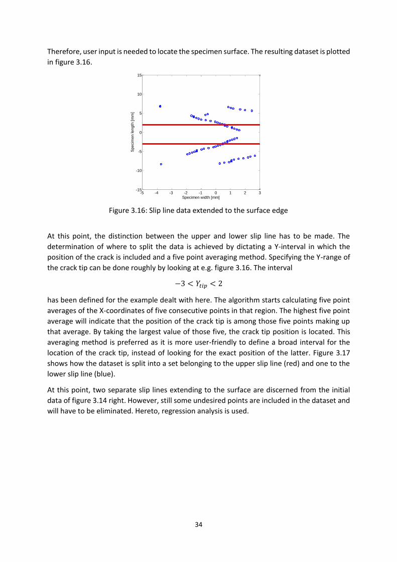
34
Therefore, user input is needed to locate the specimen surface. The resulting dataset is plotted
in figure 3.16.
Figure 3.16: Slip line data extended to the surface edge
At this point, the distinction between the upper and lower slip line has to be made. The
determination of where to split the data is achieved by dictating a Y-interval in which the
position of the crack is included and a five point averaging method. Specifying the Y-range of
the crack tip can be done roughly by looking at e.g. figure 3.16. The interval
−3 < 𝑌𝑡𝑖𝑝 < 2
has been defined for the example dealt with here. The algorithm starts calculating five point
averages of the X-coordinates of five consecutive points in that region. The highest five point
average will indicate that the position of the crack tip is among those five points making up
that average. By taking the largest value of those five, the crack tip position is located. This
averaging method is preferred as it is more user-friendly to define a broad interval for the
location of the crack tip, instead of looking for the exact position of the latter. Figure 3.17
shows how the dataset is split into a set belonging to the upper slip line (red) and one to the
lower slip line (blue).
At this point, two separate slip lines extending to the surface are discerned from the initial
data of figure 3.14 right. However, still some undesired points are included in the dataset and
will have to be eliminated. Hereto, regression analysis is used.
-5 -4 -3 -2 -1 0 1 2 3-15
-10
-5
0
5
10
15cell F
Specimen width [mm]
Specim
en length
[m
m]

35
Figure 3.17: Split of the data in a upper (red) and lower (blue) slip line
From the crack tip onwards, both the upper and lower slip line data are checked for the longest
group of consecutive points for which their X-coordinate does not differ more than 1.5 times
the grid spacing in the X-direction (Δx, see section 3.3) from each other. In most cases, i.e.
when other strain paths are not dominating, this will result in the detection of the main slip
line. A regression line is fitted to that specific group of points that belong to the main slip line.
By doing this search for the main slip line, the situation in figure 3.18 right is obtained instead
of the one on the left hand side. Clearly, the regression was successful on the right, while that
on the left is influenced by the points that have to be eliminated.
Figure 3.18: Slip lines and regression lines before elimination
For the regression analysis, the maximum power of the regression line is defined by the user.
The algorithm tries all regression lines up to the maximum power and selects the one best
fitting the data. However, also one specific polynomial degree can be specified. From this
regression line, the vertical distance to all points is checked and compared to the maximum
allowed distance defined by the user. When exceeding the value set by the user, the points
-5 -4 -3 -2 -1 0 1 2 3-15
-10
-5
0
5
10
15cell G
Specimen width [mm]
Specim
en length
[m
m]
-5 -4 -3 -2 -1 0 1 2 3-15
-10
-5
0
5
10
15Before elimination (cell G)
Specimen width [mm]
Specim
en length
[m
m]
slip line
regression line
-5 -4 -3 -2 -1 0 1 2 3-15
-10
-5
0
5
10
15Before elimination (cell G)
Specimen width [mm]
Specim
en length
[m
m]
slip line
regression line

36
are eliminated. The user can also specify to keep the end points of the slip line at the surface
edge out of this calculation. Figure 3.19 shows how the elimination turned out for either
situations of figure 3.18. Clearly, for the case at the right, slip line points have been eliminated
and the regression was not successful. The regression line can also not reposition itself to
better fit the main trend of the remaining data as the algorithm to look for the main trend is
not implemented for the left hand side. At the right, the points have been deleted correctly
and the desired slip lines are recovered completely.
Figure 3.19: Slip lines and regression lines after elimination
3.5.2. Numerical At Soete Laboratory a Python™ script has been developed for the creation of 3D finite element
models of a SENT specimen with a stationary (non-growing) crack in ABAQUS®. Customized
modelling of this SENT specimen is facilitated with the use of an object-oriented approach
script that automatically generates a batch of desired models. The same script also has
extended post-processing procedures implemented. One function postProcessSlipLine() has
been added to this Python™ script for the extraction of slip line data. For an in depth discussion
of the added code, the reader is referred to appendix B. The reader is referred to reference
[1] for a more detailed description of the complete SENT script.
When carrying out a simulation with the SENT script in ABAQUS®, the following steps are
followed.
1. Create a Python™ input file
2. Generate the model
3. Execute the finite element simulation
4. Post process the simulations to generate general output
5. Post process the simulations to generate slip line related output
Step five has been added in the framework of this thesis. Each step is briefly discussed below.
-5 -4 -3 -2 -1 0 1 2 3-15
-10
-5
0
5
10
15After elimination (cell H)
Specimen width [mm]
Specim
en length
[m
m]
slip line
regression line
-5 -4 -3 -2 -1 0 1 2 3-15
-10
-5
0
5
10
15After elimination (cell H)
Specimen width [mm]
Specim
en length
[m
m]
slip line
regression line

37
Creation of the Python™ input file
Start: excel spreadsheet obtain: Python™ parameter input file
In order to perform the simulation of this SENT.py script, a Python™ parameter input file has
to be generated. This file defines a Python™ dictionary containing the value of each input
parameter. For the sake of slip line extraction, five extra input parameters have been added,
which are summarized in table 3.6. The Python™ parameter files result from converting an
excel spreadsheet, listing all parameters, with Matlab®.
Generate the model and execute the finite element simulation
Start: Python ™ parameter input file obtain: simulation output files (.odb files)
ABAQUS® reads the parameter files to generate input (.inp) files using the command
<variableName>.preProcess(). By moving the .inp files into the folder containing the Matlab®
script GenerateBatchFile.m, a batch file is obtained. Place the batch file and its corresponding
input files in a random folder and execute the batch file to start the simulation.
Post-process the simulations to obtain general output files (not including slip line output
files)
Start: .odb output files obtain: Output text files (all but the slip line data)
Once concluded, each simulation will have returned an output .odb file. The simulation can be
post-processed by the command <variableName>.postProcess() in ABAQUS®. Various text
files will be created according to the post processing procedures that have been implemented
in the SENT.py file. An important file in that respect is the file named ‘_output’ including
among others the time, force and CTOD values. Another useful file with simulations is the
status file .sta reporting the convergence history of the simulations.
Post-process the simulation to obtain slip line data
Start: .odb output files obtain: Slip line output files
Slip line evaluation of the simulations is activated separately with the
<variableName>.postProcessSlipLine() command. What results is a .csv file for each
simulation. Each .csv file contains slip line data, extracted at specific increments. These
instants are determined by the parameter ‘slipLineFrameInterval’ from table 3.6. Finally, the
parameter ‘closeOdb’ states whether the output file is closed after each post processing of a
simulation. For large batches, this can be useful as too many open output files can slow down
the computer and finally let ABAQUS® crash due to a lack of available RAM memory.

38
Table 3.6: Slip line input parameters
Input parameter slip line post-processing Description
isSlipLineAnalysis Activate the slip line analysis (True/False)
slipLineNrOfGridLines Nr. of grid lines at each side of the crack
slipLineDistanceGridLines Distance between two consecutive grid lines
slipLineFrameInterval Interval of frames at which the slip line pattern is evaluated
closeOdb Close the odb. file after analysis (True/False)
3.5.2.1. Python™ implementation of slip line analysis
The slip line analysis is activated with the parameter ‘isSlipLineAnalysis’. In ABAQUS®
equivalent plastic strain according to the theory derived in section 3.2 is given by the variable
‘PEEQ’. It is this variable that will be used in the determination of the slip line coordinates.
Figure 3.20: Path definitions and coordinate system
Define the paths used for data extraction
At each side of the crack tip, a specified number of lines with a fixed distance with respect to
each other is created (figure 3.20). The number of grid lines at each side is specified by the
input variable ‘slipLineNrOfGridLines’ (𝑁 in figure 3.20), while the distance is set at
‘slipLineDistanceGridLines’ (𝐷 in figure 3.20). Remark that the SENT specimen can contain side
grooves and hereto the grid lines need to be sufficiently removed from the side groove center.
Numerical discretization caused the cells to be chamfered at the side groove edge (arc in figure
3.21), and therefore a very low value of 0.001 was added to the side groove radius used in the
path definitions compared to the true radius of the side groove in the model. Without this
small value, the first grid line (N°1 in figure 3.21) would be floating in free space, leading to an
error in ABAQUS® when the slip line analysis is started. Furthermore, the shape of the path is
set at ‘undeformed’. During the simulation, the specimen will deform. However, the path will
always be defined as if the specimen is undeformed, i.e. with respect to the coordinates of
the specimen in its initial, undeformed shape.
Y
X
DN Side groove

39
Figure 3.21: Mesh chamfer along the side groove edge
After defining the paths, a .csv file is generated for that specific simulation. Table 3.7 shows
the global structure of the .csv file, which is similar to that for data originating from VIC3D®,
but here an increment is the equivalent for a ‘image’ with the DIC software.
Table 3.7: Structure .csv file with ABAQUS®
Increment X [mm] Y [mm] U [mm] V [mm] 𝑈𝐶 𝑉𝐶 PEEQ
1 - 0.1 … … … … … … 1 0.1 … … … … … … 1 -0.2 1 0.2 ⋮ ⋮ 1 -19.9 … … … … … … 1 19.9 … … … … … … 1 -20.0 … … … … … … 1 20.0 … … … … … …
21 -0.1 … … … … … … 21 0.1 … … … … … … ⋮ ⋮
21 -20.0 … … … … … … 21 20.0 … … … … … …
⋮ ⋮
201 -0.1 … … … … … … 201 0.1 … … … … … …
⋮ ⋮ 201 20.0 … … … … … … 201 20.0 … … … … … …
Starting for increment 1, after each ‘slipLineFrameInterva’l number of increments, a new
evaluation of the slip lines will be performed. The data for each evaluation is added
consecutively to the file. Each increment will cover two times ‘slipLineNrOfGridLines’ rows.
Table 3.7 shows an example in which the two first grid lines are originated at a distance 0.1
from the crack center. First data for the grid line to the left of the crack (negative X-values in
figure 3.20) is written and afterwards for the grid line to the right (positive X-values in figure
N°1

40
3.20). Moreover, the grid lines are removed by 0.1 from each other, meaning that each side
will have 200 grid lines, so a total of 400 lines will be encompassed in one slip line evaluation.
This example stops at increment 201, and the evaluation is repeated every 20 increments.
Table 3.8 summarizes the input variables that would give rise to the example cited in table
3.7.
Table 3.8: Input parameters for example table 3.7
Input parameter Value for example in table 3.5
isSlipLineAnalysis True
slipLineNrOfGridLines 200
slipLineDistanceGridLines 0.1
slipLineFrameInterval 20
closeOdb True or False
From the defined paths, the slip lines can be determined. Each path intersects the mesh at
multiple locations. The intersection at which the ‘PEEQ’ value is maximum for that path is part
of the slip line and therefore the coordinates, displacements and ‘PEEQ’ are stored for that
intersection point. Repeating this search for each path will result in the locations that
constitute the slip lines.
Remark that in contrast to the experimental data, the maximum is determined before writing
the slip line data to the .csv file, as this is possible with ABAQUS® but not with the DIC software.
This will significantly reduce the data manipulation for the simulations in Matlab® in a later
stage (see appendix B).
Extract the data
All paths along which data has to be attained are defined. Starting at the crack tip, the
displacements 𝑈 and 𝑉, named 𝑈𝑐 and 𝑉𝑐 for the crack are obtained. Also the coordinates,
displacements 𝑈 and 𝑉 and strain ‘PEEQ’ are extracted at the slip line locations.
Eventually, the acquired data is put in their corresponding arrays and written to a .csv file with
the structure shown in table 3.7.
3.6. Validation of experimental and numerical implementation This section checks the agreement of the experimentally and numerically obtained slip lines
in section 3.5. Both experimental as numerical ‘dummy’ tests have been performed. These
tests did not contain a weld and can therefore be considered as fully homogeneous.
Homogeneous material is used as the results can then be compared with theoretical outcomes
suggested in section 3.2. Both for the experimental and numerical analysis, two specimens
have been tested, one with side grooves (5% width reduction per side groove) and one without
side grooves. By doing so, the influence of side grooves on the slip line pattern can be verified.
3.6.1. Dummy experiments The two SENT test specimens were extracted from API-5L X70 high strength pipeline steel.

41
The SENT tests were performed on a 150 kN hydraulic universal test rig at the laboratory and
digital image correlation (DIC) was used to track the strains at the surface, as described in
chapter 4. The specimens had a square cross section with 𝐵 and 𝑊 equal to 12.5 mm, a total
length of 225 mm and the clamped daylight length amounted to 10 times the width (figure
3.21). As mentioned above, the side grooves reduced the specimen width by 5% each. The
initial notch had a relative depth a0/W of 0.3 for both specimens and a notch tip radius of 75
μm, obtained through milling.
Figure 3.22: SENT geometry
The test procedure was performed according to an unloading compliance procedure
As explained in section 3.3, the grid resolution for the extraction of data from DIC is set at 50
points in the X-direction and 200 in the Y-direction. The crack tip opening is measured
according to the δ5 method.
3.6.2. Dummy simulations The simulations of the ‘dummy’ specimens were performed in the finite element software
with the SENT script as described in section 3.5.2. The material properties of the specimens
used in the experimental setup are determined with supporting uniaxial tension tests. The
parameters obtained from those tests are implemented in the SENT model in ABAQUS® (see
chapter 5) and the material properties are modelled homogeneous over the entire specimen.
3.6.3. Results The slip line angles of both tests and simulations have been determined with linear regression
analysis. The results for the specimen without side grooves are plotted on the left hand side
of figure 3.23 and for the grooved specimen on the right hand side of that figure. The top and
bottom slip line refer to the experimental results while only one angle is drawn for the
simulations. Indeed, as the specimen is symmetric and has homogeneous material properties
the angles of both simulated slip lines are equal. First it should be noted that final CTOD for
the simulations is only about half of that for the experiments.
10W
W
A A
0.9B
View A-A
B
Side groove

42
Figure 3.23: Slip line angles for the specimen without side grooves (left) and with side
grooves (right)
With the experimental results, the slip line angles of top and bottom slip line are close. This is
indeed expected for homogeneous material (equal in the ideal case). Furthermore, the angle
tends to increase somewhat for CTOD values above 1.5 mm. The reason for this behaviour will
be extensively discussed in chapter 6. Furthermore, the slip line angle varies around 50°. From
theory, it is expected that this angle would be 45° in homogeneous material. This 5° difference
is related to the deviation of the slip line from its linear trend when approaching the surface
(figure 3.24). If only the linear trend would be observed, the angle varies around 45° as
expected, as shown in figure 3.25. Finally, the experiments do not seem to indicate that side
grooves have an effect on the slip line angle. However, the simulations do show an effect.
The slip line angle for the simulations increases with around 3° when the specimen is side
grooved, from around 51° for the non-side grooved specimen to around 54° for the side
grooved specimen (again if only the linear trend is analyzed, the angle remains around 45° for
both specimens). Also, the slip line angle remains constant during most of the simulation. This
constant angle is acknowledged when observing the graphs in figure 3.24. They show in blue
the slip lines at the start of the simulation and in red those at the end of the simulation. Their
respective linear regression lines are colored green.
0 0.5 1 1.5 20
10
20
30
40
50
60
CTOD (mm)
Slip
lin
e a
ngle
(°)
top slip line
bottom slip line
slip line simulation
0 0.5 1 1.5 20
10
20
30
40
50
60
CTOD (mm)
Slip
lin
e a
ngle
(°)
top slip line
bottom slip line
simulation slip line

43
Figure 3.24: Simulation slip lines without side grooves (left) and with side grooves (right)
Figure 3.25: Slip line angles of the linear trend for the specimen without side grooves (left)
and with side grooves (right)
The difference in angle for the side grooved and non-side grooved simulations can be
explained when studying the propagation behaviour of the plastic region during the
simulations. Figures 3.26 and 3.27 show the equivalent plastic strains at the end of each
simulation.
-10 -5 0-10
-8
-6
-4
-2
0
2
4
6
8
10Slip line paths during a SENT simulation
Specimen width [mm]
Specim
en length
[m
m]
start simulation
end simulation
regression start
regression end
-10 -5 0-10
-8
-6
-4
-2
0
2
4
6
8
10Slip line paths during a SENT simulation
Specimen width [mm]
Specim
en length
[m
m]
start simulation
end simulation
regression start
regression end
0 0.5 1 1.5 20
10
20
30
40
50
60
CTOD (mm)
Slip
lin
e a
ngle
(°)
top slip line
bottom slip line
simulation slip line
0 0.5 1 1.5 20
10
20
30
40
50
60
CTOD (mm)
Slip
lin
e a
ngle
(°)
top slip line
bottom slip line
simulation slip line

44
Figure 3.26: PEEQ in the specimen without side grooves
In the specimen without side grooves, the plastic region at the notch grows more in the
direction perpendicular to that notch before turning towards the surface as slip lines.
Consequently, slip lines are pushed more aside before turning towards the surface. For the
specimen with side grooves, the groove undergoes a large part of the plastic deformation. Slip
lines can grow freely. For a more detailed analysis, the reader is referred to chapter 6.
Figure 3.27: PEEQ in the specimen side grooved specimen
Finally, it can be concluded that the results of the methods elaborated in this chapter for
experiments and simulations comply closely and can be applied together for further analysis
of slip lines in SENT specimens.
3.7. Conclusions In this chapter the theory of slip line fields is briefly outlined. An algorithm has been
established to visualize slip lines for both SENT experiments with DIC analysis, as for SENT
simulations in ABAQUS®. The slip lines can be subjected to a regression analysis which is used
to characterize their path through the specimen thickness. Hence, slip line angles can be
defined. The scripts to visualize and characterize the slip lines for both experiments and
simulations have been implemented in Matlab®. The agreement of the numerical and
experimental results has been evaluated successfully.

45
Chapter 4 Experimental work 4.1. Introduction The previous chapter introduced the post processing techniques to evaluate slip line paths in
SENT experiments. As outlined in chapter two, the main goal of this work is to link slip line
behaviour with weld heterogeneity. This chapter focuses on the experiments that are
performed on welded material and for which full field strain distributions are tracked with DIC.
In total three weld series, each originating from a different weld and base material, are tested.
Section 4.2 describes the material that is used in the experiments, while the test preparation
is discussed in section 4.3. Tension tests can be performed according to various procedures.
Therefore section 4.4 is devoted to the procedure characteristics and the test bench setup.
4.2. Test material The test material originates from steel samples that date back to the 1960s and 1970s. The
samples are extracted from curved plates taken out of pipelines and are approximately 380 x
360 mm large. The steel samples are divided into four series: 1, 2, 3 and 4. Each sample
contains a circumferential weld and connects two different pipes, “pipe 1” and “pipe 2”. Series
1 and 3 have a nominal thickness of 10.2 mm, while this is 12.2 mm for series 2 and 4.
The samples have a steel grade of API 5L X60. The following basic characterisation tests have
been performed for more detailed mapping of the material properties.
Uniaxial tension tests
Hardness tests
Uniaxial tension tests supplied the stress-strain properties of the materials, both of the pipes
as of the weld material. The tensile tests have been performed in the pipes transverse
direction. The stress-strain data for the two connecting pipes of each weld, together with the
data for the weld itself are summarized in table 4.1. Weld series 1 is not mentioned in that
table, as this material will not be used in this thesis work. The characterization of pipe 2 for
series 4 was not completely successful as the specimen was already plastically deformed at
the start of the test. Therefore, the only reliable outputs were E and tensile strength Rm.
Figures 4.1, 4.2 and 4.3 show the stress-strain curves for each series separately.

46
Table 4.1: Material properties of the base and weld material (*) not all data could be obtained as the specimen already plastically deformed at the start
of the test
Series Base
metal/ weld
Pipe (1,2)
E (MPa)
Yield strength Tensile
strength Y/T (-)
Uniform elongation
uEl (%) Rp0.2
(MPa) Rt0.5
(MPa) Rp1.0
(MPa) Rm
(MPa)
2 BM
1 196723 440.35 442.50 446.72 630.85 0.698 13.90
2 199050 432.79 434.99 444.64 619.05 0.699 14.69
Weld 195147 522.71 524.30 540.29 651.68 0.802 9.86
3 BM
1 215861 428.90 437.01 468.07 592.34 0.724 13.43
2 215601 449.80 455.31 484.05 592.34 0.759 15.02
Weld 212277 581.37 583.76 596.92 696.56 0.835 7.84
4 BM
1 202493 541.53 541.63 561.99 654.57 0.827 10.37
2* 189970 - - - 594.42 - -
Weld 245239 588.88 593.96 604.65 717.26 0.821 11.01
Figure 4.1: Stress-strain curve for weld series 2
Figure 4.2: Stress-strain curve for weld series 3
0
100
200
300
400
500
600
700
0 5 10 15 20
Engi
nee
rin
g st
ress
(M
Pa)
Engineering strain (%)
2-1
2-2
2-W
0
100
200
300
400
500
600
700
800
0 5 10 15 20
Engi
nee
rin
g st
ress
(M
Pa)
Engineering strain (%)
3-1
3-2
3-W
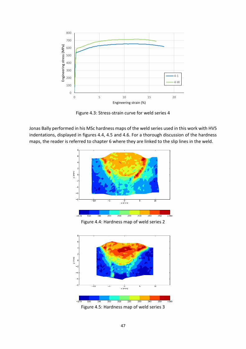
47
Figure 4.3: Stress-strain curve for weld series 4
Jonas Bally performed in his MSc hardness maps of the weld series used in this work with HV5
indentations, displayed in figures 4.4, 4.5 and 4.6. For a thorough discussion of the hardness
maps, the reader is referred to chapter 6 where they are linked to the slip lines in the weld.
Figure 4.4: Hardness map of weld series 2
Figure 4.5: Hardness map of weld series 3
0
100
200
300
400
500
600
700
800
0 5 10 15 20
Engi
nee
rin
g st
ress
(M
Pa)
Engineering strain (%)
4-1
4-W

48
Figure 4.6: Hardness map of weld series 4
4.3. Test program As mentioned in the previous section, series 2, 3 and 4 have been selected in this work for
SENT testing based on Soete Laboratory’s in-house developed test procedure. From each
weld, ten SENT specimen bars have been cut. Out of these 30 specimens, nine specimens were
prepared for testing, three of each series. Preparing the specimens geometrically
encompasses the decision of where in the weld the notch is applied and whether the
specimens have to be side grooved. Table 4.2 presents the latter for the selected specimens.
The table also indicates whether the specimens were indeed tested. With two specimens,
problems occurred before or after testing. Namely when removing specimen 3.2 from the test
rig, the test rig computer ran into a blocking status as the hydraulic piston was mishandled.
Therefore the reset button was applied leading to an erase of the analog data of that test. In
the light of that event, the correct procedure was not activated for the next test. The test rig
consequently executed a false procedure. Even intervening a couple of seconds after the test
was started could not avoid the specimen from being destroyed. Consequently, for specimen
3.2 only DIC data has been attained, while for specimen 3.3 no test data at all has been
obtained.
Table 4.2: Overview of the specimens prepared for testing (*WMC = weld metal center, AD = analog test bench data)
Specimen Notch location* Side grooved? Tested?*
2.1 WMC yes yes
2.2 WMC yes yes
2.3 WMC yes yes
3.1 WMC yes yes
3.2 WMC yes yes (no AD)
3.3 WMC yes no
4.1 WMC yes yes
4.2 WMC yes yes
4.3 WMC yes yes

49
In table 4.3 the principal dimensions of the specimens are reported. The width 𝑊 (dimension
in the direction of the initial crack) and thickness 𝐵 were determined using a micrometer,
measuring at three equally spaced points along the specimen centerline. The length 𝐿 of each
specimen was estimated with the help of a caliper.
Table 4.3: Dimension measurements of the prepared specimens
Specimen Width 𝑊 (mm) Thickness 𝐵 (mm) Length 𝐿
(mm) 1 2 3 Average 1 2 3 Average
2.1 9.67 9.71 9.72 9.70 9.7 9.71 9.71 9.71 240
2.2 9.67 9.72 9.71 9.70 9.65 9.70 9.70 9.68 240
2.3 9.70 9.70 9.75 9.72 9.70 9.64 9.67 9.67 240
3.1 8.96 9.00 9.01 8.99 8.94 8.96 8.97 8.96 200
3.2 8.93 8.93 8.94 8.93 8.95 8.93 8.95 8.94 200
3.3 8.99 8.94 8.99 8.96 8.96 8.98 8.97 8.98 200
4.1 9.67 9.65 9.64 9.65 9.59 9.61 9.62 9.61 240
4.2 9.62 9.62 9.62 9.62 9.57 9.55 9.59 9.57 240
4.3 9.58 9.63 9.63 9.61 9.60 9.59 9.58 9.59 240
4.3.1. Preparation of the specimens In order to make the raw specimen ready for testing the following steps were followed:
Machining of side grooves to all specimens
Notch the specimens to a predefined initial crack depth
Drill holes for the attachment of the clip gauge knifes
Provide the specimens with a speckle pattern for DIC analysis
4.3.1.1. Machining side grooves
The side grooves were machined with a milling cutter device at the laboratory. The position
of the side grooves has been chosen such that their root coincides with the initial notch
section. Side-grooves are applied at both sides of that notch section and each of them reduces
the specimen width by 5%. The depth of a side groove for each specimen is summarized in
table 4.4.
Table 4.4: Depth of the side grooves
Weld series Side groove depth ℎ𝑔𝑟𝑜𝑜𝑣𝑒 (mm)
2 0.48
3 0.45
4 0.48
4.3.1.2. Notching the specimen
The specimens were notched to a predefined initial crack depth a0 with the use of a circular
saw, creating a notch tip radius of 75µm. The initial crack depth varies for each specimen and
is specified by the dimensionless ratio a0/W. In each test series notch depth values a0/W were
aimed towards 0.2, 0.3 and 0.4 for the following reason. It is beneficial for the study of slip
line behaviour in relation to the microstructure, that the slip lines cross as many

50
microstructures on their way to the specimen surface. The a0/W position defines the onset of
the crack growth and by assuming 45° propagation from that position, the number of
microstructures that are crossed can be visualized on the hardness maps. The values 0.2, 0.3
and 0.4 are found to be complying well with that stipulation. Table 4.5 gives an overview of
the initial crack depths for each specimen.
Table 4.5: Initial crack depths of the specimens
Specimen Average width W (mm) a0/W goal a0 goal (mm)
2.1 9.70 0.2 1.94
2.2 9.70 0.3 2.91
2.3 9.72 0.4 3.89
3.1 8.99 0.2 1.80
3.2 8.93 0.3 2.68
3.3 8.96 0.4 3.58
4.1 9.65 0.4 3.86
4.2 9.62 0.3 2.89
4.3 9.61 0.2 1.92
4.3.1.3. Holes for clip gauge attachment
Two clip gauges were mounted on the specimen for tracking the crack tip opening
displacement (CTOD). The clip gauge knives used for sensor attachment are drawn in figure
4.7 and figure 4.8 demonstrates the implementation of knives and sensors during a SENT test.
These clip gauges knives enable the use of two clip gauges, a lower and higher clip gauge. Both
clips are mounted directly at the specimen surface. As such the lower gauge is 2 mm above
the specimen surface, while the higher gauge is 8 mm above the surface. The fixation of a clip
gauge onto the specimen surface is assured by two self-tapping screws (type “#2-56 x 3/16”
“Phillips Pan Head Thread Cutting Screw”) of 2 mm nominal diameter. For that purpose, four
holes have to be drilled, two at each side of the notch, according to the pattern shown in figure
4.9. The drilling procedure is well described in the SENT test procedure of Soete Laboratory.
Figure 4.7: Clip gauge knives

51
Figure 4.8: Clip gauge knives and sensors during a SENT test
The 1.9 mm holes were drilled with a drill press, aiming at a depth of 2.5 mm. The position of
the holes has been visualized with the help of scratches, see figure 4.9. The notch served as
the reference for the position of the holes in the horizontal direction, while the specimen
lower edge served as the reference for the position of the holes in the vertical direction.
Figure 4.9: Position of 2.5 mm deep holes for clip gauge attachment (dimensions in mm)
Already in this phase of the test preparation, potential problems were observed with respect
to the attachment of clip gauges. The specimen width does not exceed 10 mm in all cases.
According to figure 4.9 the outer edges of the holes of a clip gauge are 7.8 mm apart.
Consequently, the holes are approximately 1 mm apart from the specimen surface for the
weld series 2 and 4 and only 0.5 mm for weld series 3. The accuracy of drilling did not meet
these requirements for all specimens. The drill press positioning mechanism experiences some
clearance, making some holes to be slightly off target. However, because of the small
specimen width, the margin for misalignment was small. Figures 4.10 and 4.11 show examples
of misalignment of the holes.

52
Figure 4.10: Drilled holes for specimen 2.2
Figure 4.11: Drilled holes for specimen 3.2
Misalignment of the holes should be avoided but is in this case exploited for improving the
strain measurements at the surface. Therefore, the close presence of the holes to the
specimen surface may influence the strain distribution at that surface and as such jeopardizes
the slip line analysis. In case of misalignment of the holes, the surface that is the farthest
removed from the holes was painted with the speckle pattern for DIC analysis.
So, the screws for the current clip gauge knives are too far apart to be applicable for specimens
with a width below 12.5 mm, an adapted clip design is proposed in the following for thinner
specimens. The considerations that have led to the design in figure 4.12 are:
The holes connecting the clip gauges of the surface should at least be 1.5 mm away
from the specimen side surface to avoid influencing the strain evolution at the surface.
The drilling depth should not exceed 2.5 mm
The same self-tapping screws, i.e. type “#2-56 x 3/16” “Phillips Pan Head Thread
Cutting Screw”, should be used for fixation of the new clip gauge knives

53
Two screws are necessary for fixation, as the pretension force would otherwise cause
the knives to rotate around their connection point.
The proposal is to reduce the distance between the two holes of the clip gauge knife. When
doing so without making other changes, the bending moment of the higher clip around the
two screws would undesirably increase. To compensate this effect partially, the holes are
moved closer towards the position of the higher clip. In order to proceed with the design, the
exact dimensions of the screws are summarized in table 4.6.
Table 4.6: Clip gauge screw dimensions
Dimension Value [mm]
Head diameter 4.25
Threaded length 4.76
Outer thread diameter 2
The head diameter of the screws determines the minimum distance between the two holes
of the clip gauge knife. With a head diameter of 4.25 mm, a distance of 5 mm was chosen
between the two centers of the holes, instead of the 6 mm of the current knives. This
reduction is minimal, but is limited due to the screw head diameter. A proposition for new clip
gauge knives is found in figure 4.12.
Figure 4.12: Proposition for new clip gauge knives
Please remind that the distance between the outer edges of both holes amounts to 7 mm with
the new knives. From the tests executed in this work, it is advised to remain at least a distance

54
of 1.5 mm to the specimen surface. Consequently, specimens having a width down to 10 mm
could be tested with the newly proposed knives.
Finally, a last remark is made regarding the penetration depth of the screws in the specimen.
The total threaded length of the suggested screws amounts to 4.76 mm. The clip is 2 mm high
at the location where the screws are applied. Hence, 2.76 mm remains and can be screwed
into the specimen. However, a maximum depth of 2.5 mm is advised by the SENT procedure
at the laboratory. Therefore the use of a M2 bolt compatible washer plate having a thickness
of about 0.5 mm is advised.
4.3.1.4. Speckle pattern
For DIC analysis, a black speckle pattern on a white background has been painted on one side
of the specimens. As explained in paragraph 4.3.1.3 the side with the largest distance to the
drilled holes has been painted in an attempt to reduce the influence of those holes on the
strain pattern at the surface.
As the speckle pattern is of major importance for good correlation of the observed strains, a
specific technique is followed through which was previously developed and optimized at Soete
Laboratory.
At first, a white ground layer is painted. To this end, apply tape to all surfaces that have not to
be painted. Next, in total three layers of white paint are applied while each layer is dried in
between by using a hairdryer. This technique assures that the layer is not reflecting and all
metal is covered sufficiently with paint. The next step is painting a black speckle pattern on
this white background. It is imperative that the speckles have the right dimensions (a speckle
size of 3 by 3 pixels is advised) and are randomly dispersed. As this step is an important but
sensitive one to mistakes, it is advised to practice painting the speckles in advance on e.g. a
piece of paper. At the time the pattern is found to be acceptable, apply the speckles on the
specimens themselves.
4.4. Test setup and procedure
4.4.1. Test setup SENT testing was performed on the Soete Laboratory’s 150 kN servohydraulic universal test
rig. Mechanical grips were used for fixation of the specimens (figure 4.13). These grips do not
allow any rotation so a “fixed grip loading” is applied. The test rig is governed by a MTS
FlexTest controlling software.

55
Figure 4.13: Experimental SENT setup on the 150 kN tension rig
When mounting the specimen, proper care has been given regarding the positioning and
orientation of the specimen. More specifically, the following points of attention are
monitored:
The daylight length of the specimen was aimed at 10𝑊, meaning that the length of
the specimen between the two grips amounts to approximately 10 times the specimen
width.
The vertical alignment of the specimen is checked with a try square
Axial alignment is assured by mounting the specimens centrally with respect to the
grip center axis. Accordingly, global bending of the specimen is avoided to the
maximum possible extent.
4.4.2. Clip gauge calibration All tests were executed in one test session. Therefore a single calibration of the clip gauge was
sufficient to cover all tests. Clip gauge calibration was performed by using a micrometer placed
in a clamp controlling the clip gauge opening. The clip gauge opening was varied from 3 mm
to 11 mm in discrete steps of 0.5 mm. This cycle was repeated 3 times, i.e. one cycle forth,
one back and a final one forth and from these values a single calibration factor is extracted
with linear regression. Clip gauge one 𝑉1 displays its values in “virtual millimeter”, while clip
gauge two 𝑉2 is expressed in Volts. The calibration factors are used to transform the readouts
of each clip gauge into physical millimeters.
Linear regression analysis has been applied to the average values of each clip gauge over the
three cycles. As can be deduced from figures 4.14 and 4.15 the following calibration factors
apply for the clip gauges (“mm” indicates virtual millimetres, mm physical millimetres):
Clip gauge 1: 0.963 “mm”/mm gives 1.03844 mm/”mm”
Clip gauge 2: 1.1012 V/mm gives 0.98081 mm/V
Clip gaugesSENT specimen
DIC cameras
Mechanical grip

56
4.4.3. Test procedure All specimens have been tested according to an unloading compliance procedure. This
procedure is implemented in the MTS FlexTest controlling software of the test rig. The
parameters of the test procedure are test specific. Below the unloading sequence is explained
and the inputs for the system are highlighted, see also figure 4.16.
Figure 4.16: Unloading compliance procedure
1. The yield limit load Py is the ‘limit load’, i.e. the maximum load for which the
deformation is estimated to remain elastic. This load is calculated with the
following equation, 𝜎0.2 being the yield strength:
𝑃𝑦 = 0.5 𝐵𝑁 𝑏0 𝜎0.2 (4.1)
with
𝐵𝑁 = 0.9 ∙ 𝐵 (4.2) 𝑏0 = 𝑊 − 𝑎0 (4.3)
2. The first five unloading cycles of the test take place in the elastic region between
0.1𝑃𝑦 and 0.5𝑃𝑦. They are performed at an actuator displacement rate of 0.002
mm/s. Prior to each unloading, the displacement rate is set to zero for five seconds.
3. Following the elastic cycles, the specimen is loaded in its plastic region at a rate of
0.005 mm/s. The time of unloading is determined by equally spaced intervals of
crack opening displacement 𝛥𝑉1 which was kept equal to or below 0.01𝑊. This
number will determine the amount of plastic unloading cycles. When testing the
different specimens, the number of cycles was found fairly small for the first two
tests (14 and 11 respectively), so the value of 𝛥𝑉1 was set to 0.005𝑊 and for the
last four tests again raised to 0.0075𝑊, see table 4.8. Again the rate of
displacement is set to zero for five seconds before unloading is started. In each
unloading, the force drops by 0.4𝑃𝑦.
4. The test is stopped when the force reaches around 80% of its maximum value.
More specifically, the point of unloading must have dropped below the 80%
Force, P
Crack Opening Displacement, V

57
threshold and the test is stopped at the rising flank of the last unloading step, i.e.
before the end of the unloading step. The latter is important regarding the
determination of the final crack depth. Ideally, the last unloading compliance cycle
complies with the determination of the final crack depth in post mortem analysis.
Should the test be stopped between two unloading cycles, this validation could not
be conducted.
Table 4.8: CMOD intervals for each test
Specimen 𝑃𝑦 (kN) ΔV1
1B-05 29.81 0.005W
1B-06 26.08 0.0075W
1B-10 22.45 0.0075W
2A-04 25.60 0.005W
2A-06 22.11 0.0075W
2A-08 19.08 0.0075W
2B-04 22.63 0.01W
2B-05 26.24 0.005W
2B-10 29.92 0.01W
4.4.4. Post mortem analysis The post mortem analysis aims at investigating the fracture surface. Therefore the specimens
are heat tinted in an oven for 2 hours at 220°C. Heat tinting causes the fractured surfaces to
corrode. Subsequently the specimens are quenched in liquid air and broken in three-point
bending with a hydraulic press. The fracture surfaces are very sensitive to corrosion. It is
imperative to maintain a good contrast between the cracked ligament during testing and the
rest ligament that is broken brittle with the hydraulic press. Therefore an anti-corrosive spray
is applied for corrosion protection of the rest ligament after brittle fracture.
Next, the specimen surfaces are examined with an optical microscope and composite pictures
are taken (see appendix for all crack surface pictures). These pictures clearly reveal the
presence of porosities and inclusions. These irregularities could hamper the interpretation of
the test results, as discussed in chapter 6.
The final crack depth is determined with the nine point average method. Nine equidistant lines
are drawn centered about the specimen centerline and a distance 0.005𝑊 removed from the
side-groove root. The crack depth, both initial as final, is determined by measuring the
distance of the crack at these points towards the specimen edge as shown in figure 4.17. The
green color indicates the initial crack while red the final crack. The width of the specimen at
its basis was used for the calibration of the length scale as this distance can be accurately
measured with a caliper

Table 4.7: Clip gauge calibration
Micrometer (mm) Series V1 (mm) V2 (V) series V1 (mm) V2 (V) series V1 (mm) V2 (V)
3.0
1 forth
-3.5086 -3.9560
1 back
-3.530 -3.9480
2 forth
-3.5340 -3.9410
3.5 -2.9900 -3.4040 -3.0440 -3.3080 -3.0190 -3.3670
4.0 -2.4998 -2.8520 -2.5580 -2.7220 -2.5235 -2.8100
4.5 -2.0123 -2.3050 -2.0770 -2.1290 -2.0370 -2.2410
5.0 -1.5320 -1.7540 -1.6020 -1.5550 -1.5520 -1.6840
5.5 -1.0544 -1.2070 -1.1240 -0.9850 -1.0690 -1.1310
6.0 -0.5791 -0.6654 -0.6490 -0.4270 -0.5915 -0.5630
6.5 -0.1030 -0.1190 -0.1750 0.1320 -0.1150 -0.0160
7.0 0.3705 0.4190 0.3010 0.6710 0.3620 0.5390
7.5 0.8460 0.9770 0.7780 1.2210 0.8390 1.0778
8.0 1.3220 1.5250 1.2590 1.7570 1.3210 1.6210
8.5 1.8030 2.0760 1.7405 2.2880 1.7990 2.1670
9.0 2.2830 2.6265 2.2243 2.8150 2.2870 2.7115
9.5 2.7650 3.1705 2.7160 3.3410 2.7675 3.2530
10.0 3.2470 3.7220 3.2580 3.8660 3.2530 3.7930
10.5 3.7360 4.2655 3.7100 4.3870 3.7340 4.3420
11.0 4.2170 4.9450 4.2114 4.9250 4.2250 4.9220
Figure 4.14: Calibration clip gauge 1 Figure 4.15: Calibration clip gauge 2
y = 0,963x - 6,39R² = 1
-4
-2
0
2
4
6
0 2 4 6 8 10 12
V1
("m
m")
Physical distance (mm)
y = 1,1012x - 7,1895R² = 0,9999
-6
-4
-2
0
2
4
6
0 2 4 6 8 10 12V2
(V
)
Physical distance (mm)
58

59
Figure 4.17: Illustration of the nine point average method
From these nine measurements, a sort of weighted average value is determined with the
following equation for 𝑎𝑖 (with 𝑖 = 𝑜, 𝑓)
𝑎𝑖 =(
𝑎𝑖,1 + 𝑎𝑖,9
2 + ∑ 𝑎𝑖,𝑗8𝑗=2 )
8
(4.4)
Tables 4.9 and 4.10 contain all crack size measurements and the resulting average value
calculated with the equation above. The final crack propagation ∆𝑎 can be easily derived by
subtracting 𝑎𝑜 from 𝑎𝑓 and the result is shown in table 4.11. As specimen 3.3 was never tested,
it is not included in the post mortem analysis.
Table 4.9: Initial crack depth with the nine-points average method
Specimen a0 at intersection with line … (mm) average
(mm) 1 2 3 4 5 6 7 8 9
2.1 2.08 2.12 2.12 2.12 2.04 1.96 1.96 1.92 1.96 2.03
2.2 2.97 2.97 2.92 2.88 2.88 2.84 2.88 2.88 2.92 2.90
2.3 3.49 3.49 3.53 3.49 3.49 3.41 3.41 3.41 3.41 3.46
3.1 1.68 1.72 1.76 1.64 1.64 1.64 1.64 1.64 1.68 1.67
3.2 2.83 2.83 2.83 2.83 2.83 2.79 2.79 2.83 2.75 2.82
4.1 3.88 3.88 3.96 3.96 3.96 3.96 3.96 3.96 3.96 3.95
4.2 3.04 3.04 3.00 2.96 2.96 2.88 2.88 2.88 2.88 2.94
4.3 2.10 2.06 2.06 2.06 2.06 2.01 2.06 2.06 2.01 2.05

60
Table 4.10: Final crack depth with the nine-points average method
Specimen af at intersection with line … average
(mm) 1 2 3 4 5 6 7 8 9
2.1 4.984 5.229 5.392 5.597 5.637 5.515 4.984 4.575 4.167 5.19
2.2 5.188 5.024 5.271 5.6 5.806 5.929 5.847 5.765 6.012 5.61
2.3 5.689 5.98 5.98 5.98 6.063 6.104 6.146 6.104 6.312 6.04
3.1 3.364 3.204 3.364 3.244 3.924 4.405 4.245 4.085 4.004 3.77
3.2 6.06 6.138 6.138 6.099 6.06 5.902 5.666 5.351 5.273 5.88
4.1 4.808 5.145 5.736 5.989 6.073 6.073 6.073 6.157 6.537 6.25
4.2 4.11 4.439 4.932 5.179 5.261 5.261 5.261 5.138 4.603 4.98
4.3 6.001 6.042 6.083 6.083 6.165 6.33 6.412 6.494 6.741 5.86
Table 4.11: Final crack growth
Specimen a0 (mm) af (mm) Δa (mm)
2.1 2.03 5.19 3.15
2.2 2.90 5.61 2.70
2.3 3.46 6.04 2.59
3.1 1.67 3.77 2.10
3.2 2.82 5.88 3.06
4.1 3.95 6.25 4.20
4.2 2.94 4.98 2.03
4.3 2.05 5.86 1.92
4.5. Conclusions Nine specimens, originating from three weld series, have been selected for the experimental
study of slip lines in SENT specimens. The welds are extracted from plates dating back to the
1960s and 1970s. The SENT experiments have been performed according an unloading
compliance procedure and the strains at the side surface of the specimen have been tracked
with digital image correlation.
The specimen widths did not exceed 10 mm making the use of the current clip gauges at the
laboratory rather difficult. The screws of the clip gauge knives were located too closely to the
specimen surface and consequently distorted strain patterns at the surface may be expected.
An adapted design of the current clip gauges has been proposed.
Finally, the post mortem-analysis is introduced, meant to determine the initial and final crack
depths and following the stable crack growth.
61
Chapter 5 Finite element analysis 5.1. Introduction In this chapter, the numerical arm of this work will be covered. Numerical studies are gaining
popularity in various research domains, such as fracture mechanics. This evolution goes hand
in hand with the current rapid increase in calculation power of new computers. Numerical
simulations, provided they have been soundly experimentally validated, have several benefits,
such as time and cost, but more importantly, they feature enormous flexibility. The
possibilities in designing models with a widespread of boundary and other conditions may at
some levels exceed the capabilities of experimental tests.
Due to its flexibility, finite element analysis is used in this work as a tool to perform a
parametric study in researching slip line behaviour. At Soete Laboratory, the numerical
software package ABAQUS® is used extensively for the purpose of simulations. A numerical
model of a SENT specimen has already been developed at the laboratory [1].
The first section of this chapter covers a brief description of the numerical model of a SENT
specimen and introduces the post processing procedure for the purpose of slip line
investigation that has been implemented. This post processing procedure has been checked
for soundness with the simulations of the ‘dummy’ specimens that were covered in section
3.6. The simulations introduced in this chapter aim to investigate the influence of
homogeneous material properties and boundary conditions on the slip line evolution in SENT
specimens. They will be post processed with the model described in chapter 3 and the results
are reported in chapter 6.
5.2. Model structure At Soete Laboratory a 3D finite element model of an edge notched specimen with a stationary
(non-growing) crack has been developed for ABAQUS® during the PhD of Matthias Verstraete
[1], see figure 5.1. Customized modelling of the specimen is enabled with the use of a
parametric Python™ script that generates the desired mesh model. Geometrical and material
properties are specified in a parameter file. The following will highlight the model
specifications used in this thesis work.
Meshing is done with linear brick elements C3D8R with reduced integration schemes. The root
of this crack has been set at 0.075 mm as this approximates the radius when machining the
notch for experimental work. As advised for the sound calculation of fracture mechanics

62
parameters, the root surroundings are meshed according to a refined spider web, see figure
5.2. [1]
Figure 5.1: SENT specimen modelled in ABAQUS®
In order to limit the amount of calculations, only one half of the SENT specimen is modeled
with symmetry boundary conditions on one side surface, as the specimen is transversally
symmetric, see figure 5.3. To assure compliance with the experiments, one end of the
specimen is clamped (displacements are kept zero) and the other free end is translated in
displacement control. Rotation of the free ends is inhibited. [1]
Figure 5.2: Spider mesh around the notch tip
Geometrically, the parameters of concern in this chapter are (see figures 5.1-5.3):
Thickness B, width W and length L
Implementation of side grooves. Their depth can be specified and they are modelled
with an opening angle of 90° and root radius of 0.4 mm.
The relative crack depth a0/W
The script allows assigning different material properties to different sections of the SENT
model. This chapter focuses on modelling homogeneous materials, i.e. not containing a weld.
As such each region is specified as having equal material properties.
L
W
B

63
Figure 5.3: Symmetry plane, side groove and notch tip of the SENT specimen
5.3. Parametric study In this section a parametric study will be introduced, that aims at understanding the influence
of geometrical and material properties on the slip line evolution in homogeneous SENT
specimens.
Traditionally, field theories like slip line field theory neglect strain hardening effects of the
material, making the material to deform at a constant stress, namely the yield stress. The slip
line theory elaborated in chapter 3 also assumes plane strain deformation. Plane strain
conditions are typically found in bar forging, sheet drawing and extrusion and cold strip rolling.
These major assumptions enable a theoretical theory to be developed, but real experiments
tend to be more of complex nature. [51]
With the experiments performed in chapter 4 the strain at the specimen surface is tracked
with a camera system. Due to the nature of the test, only the surface of the specimen is
analyzed. As the surface is considered stress free, these experiments show slip line patterns
for plane stress, instead of plane strain used in the theory in chapter 3. However the theory
of slip line fields can be derived for plane stress conditions too. Hill [47] elaborated the details
for plane plastic stress and Slater [51] reported briefly the equations of plane stress with the
von Mises yield criterion. The application of the plane stress equations for the stress free
boundary condition are highlighted as well. Theoretically, the slip line in an isotropic material
in a plane stress condition should make an angle of 54.44° with the specimen surface.
The parameter study conducted in this chapter is aiming at addressing these differences of
reality with theory. Studying the influence of stress state (plane strain, plane stress) and
material properties (strain hardening, perfectly plastic) will provide information about the
validity of the theoretical solutions in SENT specimens.
Symmetry plane
Notch tipSide groove
a0
W

64
5.3.1. Parameters
For the purpose of investigating the influence of material properties, strength properties and
stress states on the slip line pattern, the following parameters have been varied in the study:
Strain hardening exponent n
The strain hardening exponent describes the course of the true stress-strain curve from
yielding until necking with the Ramberg-Osgood power law.
𝜀 =
𝜎
𝐸+ 0.002 (
𝜎
𝐸 )
𝑛
(5.1)
This equation implies that the yield strength corresponds with a plastic strain of 0.002 (0.2%).
When the strain hardening exponent n is chosen higher, the stress-strain curve will flatten, i.e.
the material will show less strain hardening. With 𝑛 = ∞ the material behaves perfectly
plastic, see figure 5.4. In this respect, four values for n have been chosen: 10, 15, 20 and 500.
Please remark that n = 500 already approaches the perfect plastic behaviour well.
Figure 5.4: True stress strain curve with Ramberg Osgood relation for varying exponent n
Young’s modulus E
The Young’s modulus is defined as the slope of the stress-strain curve in the elastic region.
The higher the Young’s modulus E, the steeper the stress-strain curve in the elastic region will
be. When E goes to infinity, the material behaves rigid, meaning that there will be no elastic
deformation, see figure 5.5. In an attempt to avoid convergence problems of the simulations,
E has been chosen equal to 20000 GPa to model the ‘rigid’ behaviour. The other value E = 200
GPa complies with the Young’s modulus of steel.
0
100
200
300
400
500
600
700
800
900
1000
0 5 10 15 20 25
σ(M
Pa)
ε (%)
n=10
n=15
n=20
n=500

65
Figure 5.5: True stress strain curve with varying Young’s modulus
Combining a high strain hardening exponent with a high Young’s modulus, results in an
approximation of the rigid-plastic material properties for which the plasticity theory in chapter
three was elaborated. These results can then be compared with those for realistic steel
properties. In this manner, it can be verified if the slip lines deviate significantly from theory
when the rigid-plastic condition is not fulfilled.
Initial crack depth a0/W
The initial crack depth is an important parameter as it influences significantly how the
uncracked ligament of the specimen is loaded. Due to the presence of a crack, the center line
of the specimen and the crack ligament do not coincide, which creates localized bending. The
amount of bending is influenced by the misalignment between these center lines or, in other
words, by a0/W. Three different values have been chosen for the initial crack depth (see figure
5.6): 0.1, 0.3 and 0.5.
Figure 5.6: Crack depth a0/W equal to 0.1 (left) 0.5 (right)
As was explained in section 5.2, the SENT model in ABAQUS® does not cope with crack growth
during testing. Consequently, the crack depth will be constant and equal to its initial value
stated by the ratio a0/W ratio that serves as an input for the simulation. In real experiments,
the crack growth will agitate the effect of localized bending as discussed in chapter 6.
0
100
200
300
400
500
600
700
0 0.1 0.2 0.3 0.4 0.5 0.6
σ(M
Pa)
ε (%)
E=200 GPa
E=20000 GPa
a0
W

66
Boundary condition/specimen geometry
Finally, the boundary conditions and specimen geometry are varied for this parameter study.
Slip line theory has been developed both for plane strain as plane stress conditions. The
correspondence with theory will be investigated by simulating both 2D plane stress and plane
strain conditions.
Figure 5.7: Overall geometry of the plane strain and plane stress specimen
A plane strain condition is simulated by reducing the specimen width to a very low value (0.001
mm) to obtain an approximate 2D simulation, see figure 5.7 and applying the correct boundary
condition, i.e. zero strain, to the surfaces perpendicular to the W dimension. Plane stress is
simulated analogously, but this time the absence of boundary conditions at the specimen
sides implies plane stress at the surface normal to the W dimension.
Figure 5.8: Overall geometry of the B = W specimen
Two SENT specimen geometries are commonly used in testing practice. This is the geometry
with the square cross section, i.e. B = W, see figure 5.8 and the geometry with a cross section
that is twice as large: B = 2W, see figure 5.9. Both geometries have been included in this
parameter study and the slip line analysis will be performed both at the specimen surface as

67
at the specimens mid-section parallel to the specimen outer surface (chapter 6). By doing this,
both plane stress respectively approximate plane strain conditions can be analyzed. The B =
W specimens have been side grooved resulting in a total width reduction of 10% (5% for each
side groove). The same absolute side groove depth has been implemented for the B = 2W
simulations, thus reducing the relative groove depth with a factor 2.
Figure 5.9: Overall geometry of the B = 2W specimen
Table 5.1: Dimensions of the simulated specimens
Simulation type
Dimension Plane strain Plane stress B = W B = 2W
𝑊 [mm] 20 20 20 20
𝐵 [mm] 0.001 0.001 20 40
𝐿 [mm] 200 200 200 200
Finally, table 5.1 and table 5.2 give an overview of all the simulations that are conducted.
Table 5.2: Overview of the simulation parameters
96 simulations in total
Plane stress Plane strain B = W B = 2W
n (-) 10, 15, 20, 500
E (GPa) 200, 20000
a0/W (-) 0.1, 0.3, 0.5
5.4. Conclusion This chapter introduced the outline of the numerical simulations performed in the light of the
parameter study. The variation of the material properties n, E and the geometrical properties
a0/W and specimen geometry for homogeneous SENT specimens, allows to investigate the
influence of those parameters on the slip line behaviour. By doing so, the deviations from
theoretical slip line evolution can be revealed and understood.

68

69
Chapter 6
Results and discussions
6.1. Introduction Chapter 4 and 5 outlined the experiments and numerical simulations that have been
performed. This chapter presents the results of both experiments and simulations. Section 6.2
discusses the experimental results, while the simulation results are presented in section 6.3.
Final conclusions are summarized in section 6.4.
6.2. Experimental results This section presents the results obtained from the SENT tests that are described in chapter
4. The final goal of this section is to understand the slip line evolution for the selected
specimens. Chapter 4 introduced the issue of the clip gauge knife holes that are positioned
too close to the surface that is analyzed with DIC. This was the case for five specimens out of
a total of nine specimens. Only specimens 2.2, 2.3, 4.1 and 4.2 did not show excessive
distortion of the strain pattern due to the clip gauges, so that slip lines could reliable be
analyzed. As only these welds are involved in the slip line analysis, the discussion in section
6.2.2 will only describe weld series two and four.
Figure 6.1 defines upper and lower slip lines in a SENT specimen. The terminology of this figure
will be applied throughout the complete chapter. All slip line plots for the experiments
described next have to be related to figure 6.1 regarding the orientation of the slip lines with
respect to the SENT specimen.
Figure 6.1: Slip lines in a SENT experiment
-4 -2 0 2-10
-8
-6
-4
-2
0
2
4
6
8Slip lines
Y
X
F
F
Side groove notch
Upper slip line
Lower slip line

70
6.2.1. Start of the analysis The unloading compliance procedure that is used for performing these SENT experiments
prescribes five unloading cycles in the linear elastic region (see section 4.4). Afterwards, the
plastic region of the material is entered. The DIC cameras take photos of the specimen each
time an unloading cycle is started. Slip lines are not discernable during the early stages of the
test, i.e. the linear elastic and first number of plastic unloading cycles. The exact number of
cycles in the plastic region from which the slip lines are clearly present depends on the
material and test procedure. The test procedure specifies at which CMOD intervals the
unloading cycles are executed. Hence, lower CMOD intervals will result in a higher number of
cycles over the complete plastic range.
For all tests, the attachment of clip gauges resulted in an affected strain pattern at the surface.
However, for the four specimens 2.2, 2.3, 4.1 and 4.2, the effect is acceptable. The strain paths
pointing towards the clip gauge holes can be filtered out with the Matlab® code explained in
appendix A, such that in the end only the main slip lines are attained.
Figure 6.2 summarizes the last two paragraphs. On the left hand side, the locations of the
maximum equivalent strain in specimen 4.1 are plotted at the instant of a load equal to 1.01𝑃𝑦
(with 𝑃𝑦 the limit load, see chapter 4) and δ5 equal to 0.069 mm. No slip lines can yet be
discerned from the resulting data, as the points of maximum equivalent strain are still too
dispersed. However, at 1.23𝑃𝑦 (δ5 = 0.19 mm) the onset of the slip lines is visible and although
strain paths point towards the clip gauge holes, physically relevant slip lines can be extracted
with the Matlab® code.
Figure 6.2: Locations of maximum equivalent plastic strain at 1.01𝑃𝑦 and 1.23𝑃𝑦 for 4.1
Figure 6.3 presents the respective DIC images of the situations displayed in figure 6.2. On the
left hand side, two large circular strain regions are situated at each side of the notch. On the
right hand side, the green/blue coloured strain fields pointing towards the holes of the clip
gauges can be clearly distinguished.
-5 -4 -3 -2 -1 0 1 2 3-20
-15
-10
-5
0
5
10
15
20
25Locations of the points of maximum equivalent total strain received from script 1
Specimen width direction [mm]
Specim
en length
direction [
mm
]
-5 -4 -3 -2 -1 0 1 2 3-20
-15
-10
-5
0
5
10
15
20
25Locations of the points of maximum equivalent total strain received from script 1
Specimen width direction [mm]
Specim
en length
direction [
mm
]
Clip gauge influence

71
Figure 6.3: DIC images of 4.1 at 1.01𝑃𝑦 and 1.23𝑃𝑦
6.2.2. Study of the weld hardness distribution The material properties have been mentioned in chapter 4, but are recapitulated in table 6.1
for weld series 2 and 4 only.
Table 6.1: Material properties of base and weld material (*) not all data could be obtained as the specimen already plastically deformed at the start
of the test
Series Base
metal/ weld
Pipe (1,2)
E (MPa)
Yield strength Tensile
strength Y/T (-)
Uniform elongation
uEl (%) Rp0.2
(MPa) Rt0.5
(MPa) Rp1.0
(MPa) Rm
(MPa)
2 BM
1 196723 440.35 442.50 446.72 630.85 0.698 13.90
2 199050 432.79 434.99 444.64 619.05 0.699 14.69
Weld 195147 522.71 524.30 540.29 651.68 0.802 9.86
4 BM
1 202493 541.53 541.63 561.99 654.57 0.827 10.37
2* 189970 - - - 594.42 - -
Weld 245239 588.88 593.96 604.65 717.26 0.821 11.01
To have a clear overview of the hardness distribution and hence the strength in the weld,
hardness maps have been made in the master thesis of Jonas Bally for the welds that are
investigated here. The hardness maps are established with HV5 and figures 6.4 and 6.5 show
the hardness maps for weld series two and four respectively.

72
Figure 6.4: Hardness map of weld series 2
Figure 6.5: Hardness map of weld series 4
Series two shows significant higher hardness in the upper weld region. Generally, the hardness
increases from about 200 in the lower region of the weld to about 240 in the upper region,
i.e. around plus 20%. The weld is clearly overmatching with respect to the base metal
hardness.
Weld series four also has a higher hardness than the base material. The heat affected zones
are also hardened with respect to the rest of the weld, however combined with a higher
hardness in the weld center and upper weld passes.
It should be noted that for the preparation of the SENT specimens, the welds are cropped
towards a rectangular cross section. Hereto, parts of the weld top and root are cut towards
the sections shown in figure 6.6.

73
Figure 6.6: Weld section after SENT preparation: series two (left) and series four (right)
6.2.3. Analysis of the selected specimens
The following subsections will describe the results for the four selected specimens 2.2, 2.3,
4.1 and 4.2. The sequence in which the respective results are shown is analog for each
specimen:
The resistance curve with a post mortem description of the specimen
Slip line trajectory in the specimen through the course of the test
Evolution of the slip line angle with respect to the CTOD along the course of the test
Introduce the slip line paths into the hardness map of the specimen
6.2.3.1 Specimen 2.2
The general specifications characterizing specimen 2.2 are summarized in table 6.2.
Table 6.2: General properties of specimen 2.2
Weld series 𝐵 𝑊 𝑎0/𝑊
1 9.68 9.7 0.30
6.2.3.1.1. Resistance curve and post mortem analysis of specimen 2.2
Figure 6.7 shows the resistance curve of specimen 2.2. The points making up the R-curve result
from the unloading compliance cycles during the test. When curve fitting these data, the
resistance curve is obtained. The final crack propagation can be checked with the help of the
post mortem procedure described in chapter 4. This results in the final crack extension line in
figure 6.7. This figure shows that both the estimation of the initial crack depth as the final
crack extension is fair.
Figure 6.7 :Resistance curve of specimen 2.2
0
1
2
3
0 1 2 3
CTO
D (
mm
)
Da (mm)
2.2
R-curve
R-curve fit
Final crack extension
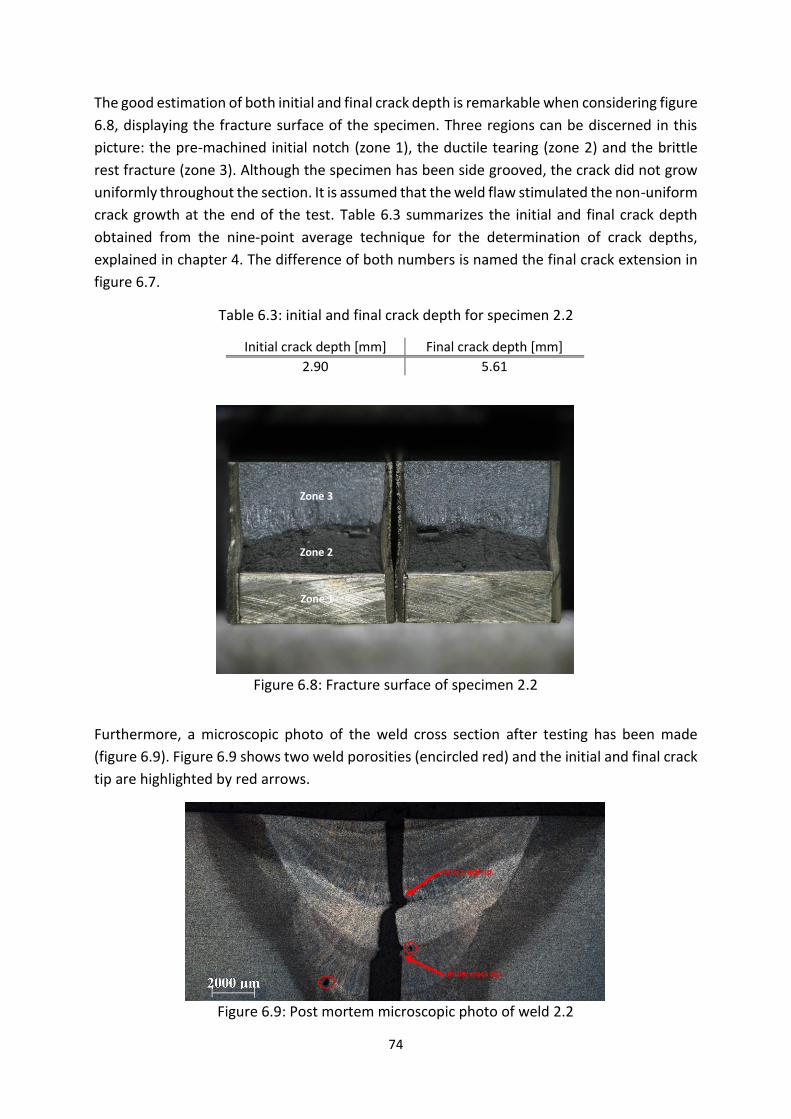
74
The good estimation of both initial and final crack depth is remarkable when considering figure
6.8, displaying the fracture surface of the specimen. Three regions can be discerned in this
picture: the pre-machined initial notch (zone 1), the ductile tearing (zone 2) and the brittle
rest fracture (zone 3). Although the specimen has been side grooved, the crack did not grow
uniformly throughout the section. It is assumed that the weld flaw stimulated the non-uniform
crack growth at the end of the test. Table 6.3 summarizes the initial and final crack depth
obtained from the nine-point average technique for the determination of crack depths,
explained in chapter 4. The difference of both numbers is named the final crack extension in
figure 6.7.
Table 6.3: initial and final crack depth for specimen 2.2
Initial crack depth [mm] Final crack depth [mm]
2.90 5.61
Figure 6.8: Fracture surface of specimen 2.2
Furthermore, a microscopic photo of the weld cross section after testing has been made
(figure 6.9). Figure 6.9 shows two weld porosities (encircled red) and the initial and final crack
tip are highlighted by red arrows.
Figure 6.9: Post mortem microscopic photo of weld 2.2
Zone 1
Zone 2
Zone 3
Final crack tip
Initial crack tip

75
6.2.3.1.2. Slip line trajectories in specimen 2.2
The slip lines in the specimen are determined with the help of the procedure reported in
chapter 3 and appendix A.
As mentioned in section 6.2.1, the start of the slip line analysis varies for each test. Here the
analysis is started with 1.19𝑃𝑦 (δ5= 0.13 mm). Figure 6.10 shows the slip line evolution in the
specimen from start (blue) until the end of the test (red) (figure 6.10 left) and only the slip line
at start (blue) and end (red) (figure 6.10 right) in the undeformed state. The slip lines are
drawn according to the concept explained in figure 6.1.
The following observations are made when studying figure 6.10
The slip lines move towards each other, i.e. the upper slip line moves in the southwest
direction of the figure, while the lower slip line moves northwest
All slip lines end at the same X-coordinate, i.e. 𝑋 = −4 in figure 6.10
The slip lines are fairly linear with the exception of the last part of the line near to the
specimen surface, which deviates from the overall linear trend
Figure 6.10: Slip lines for 2.2 in the undeformed state
The observations made above will be described next.
The crack grows during the course of the test. This crack growth is reflected in a horizontal
translation of the slip lines in figure 6.10 in the negative X-direction. This is verified by
determining the horizontal translation of the slip lines as function of the crack growth (figure
6.11). The crack growth is obtained from the R-curve fit in figure 6.7 as the CTOD value at each
slip line evaluation is known. The orange line in figure 6.11 represents 1:1 behaviour which
would prove the statement. In reality the figure fluctuates around the theoretical 1:1 curve.
-4 -2 0 2-10
-8
-6
-4
-2
0
2
4
6
8Slip lines
-4 -2 0 2-10
-8
-6
-4
-2
0
2
4
6
8Slip lines

76
The non-deformed specimen has straight surface edges. When determining the slip lines
according to that state, they must all meet the specimen surface along a straight line. In figure
6.10 the specimen surface is located at 𝑋 = −4.
Figure 6.11: The horizontal x displacement of the slip lines as function of crack growth
Finally, the deviation of the slip lines when nearing the specimen surface, indicated by the
filled and dotted circles in figure 6.10, can be explained by the bending of the specimen and
the existence of a “second strain path”. When the tensile load is applied to the specimen, a
bending moment will be generated due to the misalignment of the resulting force and the
center of the uncracked ligament of the specimen. The uncracked section will serve as a hinge
for that bending moment. Consequently, the stress state changes throughout the ligament
and the slip lines will be influenced by the latter as highlighted with a dotted circle in figure
6.10. This will be described more in detail when discussing the results for the numerical
simulations in section 6.3. The filled circle in figure 6.10 indicates a trend deviation due to the
existence of a “second strain path”. From section 6.2.2 it is learned that the weld is highly
heterogeneous. Slip line theory, however, is established for homogeneous material. The
presence of weld strength heterogeneity may provide the necessary driving force for another
strain path to develop. This means that the plasticity in the weld is not only concentrated
around the assumed upper and lower slip line. Figure 6.12 proves the existence of the
additional plastic region, here dominated as “second strain path” (encircled red in figure 6.12).
0
0.2
0.4
0.6
0.8
1
1.2
1.4
0 0.2 0.4 0.6 0.8 1 1.2 1.4
xDis
p [
mm
]
∆a [mm]
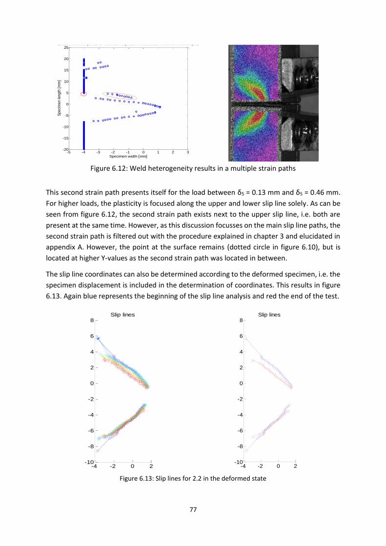
77
Figure 6.12: Weld heterogeneity results in a multiple strain paths
This second strain path presents itself for the load between δ5 = 0.13 mm and δ5 = 0.46 mm.
For higher loads, the plasticity is focused along the upper and lower slip line solely. As can be
seen from figure 6.12, the second strain path exists next to the upper slip line, i.e. both are
present at the same time. However, as this discussion focusses on the main slip line paths, the
second strain path is filtered out with the procedure explained in chapter 3 and elucidated in
appendix A. However, the point at the surface remains (dotted circle in figure 6.10), but is
located at higher Y-values as the second strain path was located in between.
The slip line coordinates can also be determined according to the deformed specimen, i.e. the
specimen displacement is included in the determination of coordinates. This results in figure
6.13. Again blue represents the beginning of the slip line analysis and red the end of the test.
Figure 6.13: Slip lines for 2.2 in the deformed state
-5 -4 -3 -2 -1 0 1 2 3-20
-15
-10
-5
0
5
10
15
20
25Locations of the points of maximum equivalent total strain received from script 1
Specimen width [mm]
Speci
men le
ngth
[m
m]
-4 -2 0 2-10
-8
-6
-4
-2
0
2
4
6
8Slip lines
-4 -2 0 2-10
-8
-6
-4
-2
0
2
4
6
8Slip lines

78
Comparing figure 6.10 to figure 6.13 it can be observed that there are both similarities as well
as differences. In figure 6.13, the slip lines have a linear trend, but again deviate from this
trend when approaching the surface. The difference is that the slip lines here do not move
inwards in the same degree as was observed in figure 6.10. The lower slip line remains almost
stationary, while the upper slip line moves slightly downwards. However, both remain
approximately at the same position with respect to the X-axis. In the deformed shape, the
specimen edge is not straight anymore but curved due to the bending moment around the
uncracked ligament and necking in that section. The curved specimen edge is also visible in
figure 6.13, as the final points of the slip lines that had an X = -4 in the non-deformed shape,
are now shifted towards higher X. This translation to the right in the figure, negates almost
completely the crack growth as the starting points of the slip lines at the notch keep
approximately the same coordinates during the test. This observation was indeed expected as
the crack tip displacement is integrated in the calculation of the slip line coordinates for the
deformed state (see chapter 3).
6.2.3.1.3. Slip line angle evolution throughout the course of the test for specimen 2.2
This section describes how the slip line angles evolve throughout the course of the test. As can
be seen in previous figures, the slip lines are fairly linear. Therefore, the linear regression
described in chapter 3 is applied for the determination of the slip line angles.
Although the main trend of the slip lines in figure 6.10 and 6.13 is linear, the points at the
intersection of the slip line with the specimen surface can deviate from that trend. As with
linear regression, a single line and hence a single slip angle is determined for each slip line, the
value for the slip line angle is biased due to those points at the surface. In the light of the weld
homogenization technique, rather the global trend of the slip line is important. The slip line
angle following from linear regression is particularly interesting to characterize the global
trend of the slip line when the points at the specimen surface are excluded. To that end, slip
line angles have also been determined in case the surface points are deleted, both for the
deformed as non-deformed state. Figure 6.14 demonstrates the result, i.e. only the linear
trend remains, for the slip lines in the undeformed state.

79
Figure 6.14: Linear section of the slip lines for specimen 2.2 in the undeformed state
Figure 6.15 plots the slip line angle versus the CTOD value at that time during the test. The left
hand side plots the angle when the complete slip line is considered, while at the left only the
angle of the linear trend is displayed. The R-curve obtained above is also implemented in the
same figure.
Figure 6.15: Slip line angle versus CTOD for the complete slip lines (left) and only the linear
trend (right) in the undeformed state
Please note that the slip line angles are plotted versus CTOD, determined with δ5 from DIC,
while the R-curve makes use of the CTOD90 values obtained with the clip gauges. Due to the
problems with the clip knife attachment as reported in chapter 4, the resulting clip gauge
signals could have been biased making the correspondence between δ5 and CTOD90 rather
poor. This remark is applicable for all figures similar to 6.15 in section 6.2.
-4 -2 0 2-10
-8
-6
-4
-2
0
2
4
6
8Slip lines
-4 -2 0 2-10
-8
-6
-4
-2
0
2
4
6
8Slip lines
0
0.5
1
1.5
2
2.5
3
3.5
0
10
20
30
40
50
60
0 1
Δa
(mm
)
Slip
lin
e a
ngl
e (
°)
CTOD (mm)
2.2
Top slip line
Bottom slip line
R-curve fit
R-curve
Final crack extension
0
0.5
1
1.5
2
2.5
3
3.5
0
10
20
30
40
50
60
0 1
Δa
(mm
)
Slip
lin
e a
ngl
e (
°)
CTOD (mm)
2.2
Top slip line
Bottom slip line
R-curve fit
R-curve
Final crack extension

80
From figure 6.15 it is clear that the angle remains approximately constant during the test and
that both left and right slip line nearly have the same slip line angle. As the angle is rather
constant, it is concluded that for this test the crack growth, visualized with the R-curve, has
no effect on the slip line angle. Table 6.4 summarizes the average angles, i.e. average over all
angles during the slip line analysis (initial 0° angle excluded), for both cases. The slip line angle
varies between 45° and 48°. The angle is 1° to 1.5° lower when only the linear trend is
observed. For the section that deviates from the global trend, the slip line angle is larger, as
such this is a logical result. The angle of the linear section only is very close to the theoretical
45°. Finally, the angle of the top slip line is somewhat higher than for the lower slip line.
However, the difference is only about 1° to 2°.
Table 6.4: Average slip line angles over the complete test for specimen 2.2
Specimen 2.2 Reference Slip line Slip line angle (°)
Complete slip line
Undeformed Top 48.04
Bottom 47.45
Deformed Top 49.26
Bottom 48.23
Linear trend only
Undeformed Top 47.84
Bottom 45.90
Deformed Top 49.50
Bottom 46.47
Table 6.4 also shows the angles of the slip lines for the deformed specimen shape. The
evolution during the test is shown in figure 6.16, in which the left hands side again represents
the angle for the complete slip line and the right hand side the angle of the linear trend only.
Figure 6.16: Slip line angle versus CTOD for the complete slip lines (left) and only the linear
trend (right) in the deformed state
6.2.3.1.4. Implementation of the slip lines into the hardness map
To conclude the discussion of the slip lines in specimen 2.2, the link between slip lines and
heterogeneity is studied. The results described above are expected to be dependent on the
weld heterogeneity. The best way to make this link is by plotting the slip lines in the hardness
0
0.5
1
1.5
2
2.5
3
3.5
0
10
20
30
40
50
60
0 1
Δa
(mm
)
Slip
lin
e a
ngl
e (
°)
CTOD (mm)
2.2
Top slip line
Bottom slip line
R-curve fit
R-curve
Final crack extension
0
0.5
1
1.5
2
2.5
3
3.5
0
10
20
30
40
50
60
0 1
Δa
(mm
)
Slip
lin
e a
ngl
e (
°)
CTOD (mm)
2.2
Top slip line
Bottom slip line
R-curve fit
R-curve
Final crack extension

81
map that is introduced in section 6.2.2. The hardness map is established according to the initial
shape of the specimen and therefore the slip lines in the non-deformed state are used to this
regard. The slip lines at the moments the load reaches 1.26𝑃𝑦 (δ5 = 0.32 mm) and 1.02𝑃𝑦 (δ5 =
0.96 mm) are shown in figure 6.17. Also the initial crack depth (thick dotted line) and final
crack depth (fine dotted line) are added. The instant when the load reaches 1.02𝑃𝑦 the test is
ended, while the other instant is chosen because of the second strain path that was in place
at that moment. The main slip lines try to go around the center of the weld which has a higher
hardness, until the crack has grown so much that the harder region is entered. When the slip
line at the right of the figure hits the strengthened heat affected zone the plasticity will start
to concentrate elsewhere, namely the second strain path is formed. This path is particularly
interesting as it exists the weld and proceeds towards the base metal of much lower strength.
The crossing through the strengthened heat affected zone is done there where the hardness
is locally lower.
Figure 6.17: Implementation of the slip lines in the hardness map of specimen 2.2
6.2.3.2. Specimen 2.3
The general specifications characterizing specimen 2.3 are summarized in table 6.5
Table 6.5: General properties of specimen 2.3
Weld series 𝐵 𝑊 𝑎0/𝑊
1 9.67 9.72 0.36
6.2.3.2.1. Resistance curve and post mortem analysis of specimen 2.3
The resistance curve of specimen 2.3 is shown in figure 6.18. The initial crack depth is
accurately predicted with the first unloading compliance cycles. However, the true final crack
extension determined with the post mortem analysis differs significantly from the crack depth
that is obtained with the last unloading compliance cycle.

82
Figure 6.18: Resistance curve of specimen 2.3
The crack did grow uniformly throughout the test as can be seen in figure 6.19. Again the
fracture surface can be subdivided into three different zones. This crack section contains a
large flaw around the point of final crack extension. This flaw could be the reason of the bad
compliance between the final crack extension from the unloading compliance procedures and
that from post mortem analysis, as the unloading compliance theory is derived for flawless
material.
Figure 6.19: Fracture surface of specimen 2.3
The initial and final crack depth determined with the nine-points averaging method are
presented in table 6.6.
Table 6.6: initial and final crack depth for specimen 2.3
Initial crack depth [mm] Final crack depth [mm]
3.46 6.04
0
1
2
3
0 1 2 3
CTO
D (
mm
)
Da (mm)
2.3
R-curve
R-curve fit
Final crack extension
Zone 1
Zone 2
Zone 3

83
The crack depths of table 6.6 are marked in the microscopic post mortem picture of the weld
(figure 6.20)
Figure 6.20: Post mortem microscopic photo of weld 2.3
6.2.3.2.2. Slip line trajectories in specimen 2.3
Compared to the slip lines in specimen 2.2, the slip lines for specimen 2.3 show similarities but
also some differences. As both specimens originate from the same weld but have a different
initial crack depth, the interaction with the weld heterogeneity is different as will be shown in
the next paragraphs. Again the distinction is made between slip lines determined according
to the deformed or non-deformed specimen state. Figure 6.21 shows the slip lines according
to the non-deformed state.
The same observations can be made as with specimen 2.2, namely:
The slip lines move towards the surface, i.e. the upper slip line moves in the southwest
direction of the figure, while the lower slip line moves northwest
All slip lines end at the same X-coordinate, i.e. 𝑋 = −4 in figure 6.21
The slip lines are fairly linear, except the last part of the line near to the specimen
surface which deviates from the overall linear trend
However, the lower slip line shows a specific behaviour that was not observed with specimen
2.2. More specifically, in the early stages of the slip line analysis, the lower slip line moves in
the southeast direction. When the load reaches 1.34𝑃𝑦 (δ5 = 0.34 mm) only the second half of
the lower slip line persists this effect and eventually, the complete slip line moves towards the
northwest in analogy with the upper slip line. It seems as if the lower slip line resists to move
inwards for as long as possible, but this becomes more difficult when the crack propagates
towards more negative X-values. Eventually, the slip line will make a jump in the northwest
direction, leaving an area uncrossed.
Final crack tip
Initial crack tip

84
Figure 6.21: : Slip lines for 2.3 in the undeformed state
The slip lines are also determined regarding the deformed specimen and plotted in figure 6.22.
The shape of the slip lines is again similar to their shape according to the non-deformed
specimen state. However, the degree in which the slip lines move inwards is higher for
specimen 2.3 compared to the slip lines in the deformed state of specimen 2.2. Although, the
lower slip line again moves less inwards than the upper slip line. The surface edge is again
curved, resulting in a translation of the slip lines towards positive X-direction when the test
proceeds. This shift compensates the crack growth and as such it seems as if the notch is nearly
stationary in figure 6.22. This translation results from including the crack tip displacement in
the calculation of the slip line coordinates in the deformed state.
Figure 6.22: Slip lines for 2.3 in the deformed state
-4 -2 0 2-10
-8
-6
-4
-2
0
2
4
6
8
10Slip lines
-4 -2 0 2-10
-8
-6
-4
-2
0
2
4
6
8
10Slip lines
-4 -2 0 2-10
-8
-6
-4
-2
0
2
4
6
8
10Slip lines
-4 -2 0 2-10
-8
-6
-4
-2
0
2
4
6
8
10Slip lines
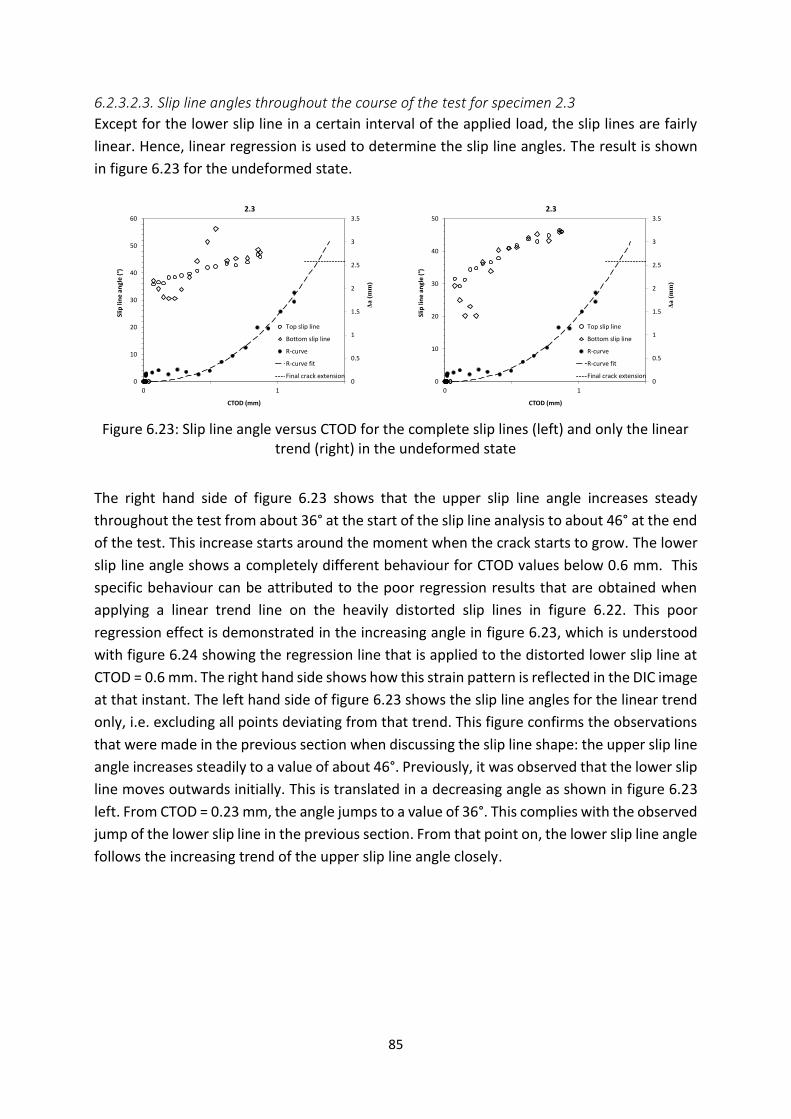
85
6.2.3.2.3. Slip line angles throughout the course of the test for specimen 2.3
Except for the lower slip line in a certain interval of the applied load, the slip lines are fairly
linear. Hence, linear regression is used to determine the slip line angles. The result is shown
in figure 6.23 for the undeformed state.
Figure 6.23: Slip line angle versus CTOD for the complete slip lines (left) and only the linear
trend (right) in the undeformed state
The right hand side of figure 6.23 shows that the upper slip line angle increases steady
throughout the test from about 36° at the start of the slip line analysis to about 46° at the end
of the test. This increase starts around the moment when the crack starts to grow. The lower
slip line angle shows a completely different behaviour for CTOD values below 0.6 mm. This
specific behaviour can be attributed to the poor regression results that are obtained when
applying a linear trend line on the heavily distorted slip lines in figure 6.22. This poor
regression effect is demonstrated in the increasing angle in figure 6.23, which is understood
with figure 6.24 showing the regression line that is applied to the distorted lower slip line at
CTOD = 0.6 mm. The right hand side shows how this strain pattern is reflected in the DIC image
at that instant. The left hand side of figure 6.23 shows the slip line angles for the linear trend
only, i.e. excluding all points deviating from that trend. This figure confirms the observations
that were made in the previous section when discussing the slip line shape: the upper slip line
angle increases steadily to a value of about 46°. Previously, it was observed that the lower slip
line moves outwards initially. This is translated in a decreasing angle as shown in figure 6.23
left. From CTOD = 0.23 mm, the angle jumps to a value of 36°. This complies with the observed
jump of the lower slip line in the previous section. From that point on, the lower slip line angle
follows the increasing trend of the upper slip line angle closely.
0
0.5
1
1.5
2
2.5
3
3.5
0
10
20
30
40
50
60
0 1
Δa (
mm
)
Slip
lin
e a
ngl
e (
°)
CTOD (mm)
2.3
Top slip line
Bottom slip line
R-curve
R-curve fit
Final crack extension0
0.5
1
1.5
2
2.5
3
3.5
0
10
20
30
40
50
0 1
Δa (
mm
)
Slip
lin
e a
ngl
e (
°)
CTOD (mm)
2.3
Top slip line
Bottom slip line
R-curve
R-curve fit
Final crack extension

86
Figurer 6.24: Poor regression analysis for the distorted lower slip line
Table 6.7 presents the average slip line angles (average over all angles during the slip line
analysis but initial 0° angle excluded), for both cases, again when considering the complete
slip line and when looking at the linear trend only. For the upper slip line the angle amounts
to about 41° for the complete slip line and about 39° for the linear trend only. Again the
difference is small (only 2°) but an angle of 39° is deviating significantly from the theoretical
45°. Again the weld heterogeneity comes into play and has its influence on the slip line
trajectory. For the bottom slip line, the resulting averages are less reliable (due to the poor
regression for a large part of the test) and do not describe the true behaviour of the slip lines.
Table 6.7: Average slip line angles over the complete test for specimen 2.3
Specimen 2.3 Reference Slip line Slip line angle (°)
Complete slip line
Undeformed Top 40.81
Bottom 41.28
Deformed Top 42.24
Bottom 41.40
Linear trend only
Undeformed Top 38.54
Bottom 35.68
Deformed Top 38.84
Bottom 35.63
For the slip lines in the deformed state, the slip line angles are slightly higher (1.5° for the
complete top slip line deformed, compared to the complete slip line undeformed) or equal
(compare the top slip line angles for the linear trend only). Again the average angles of the
lower slip line are less reliable. Figure 6.25 shows the plot of the slip line angles for the
deformed state. It is again observed that the evolution is equal to that in the undeformed
state, as the shape of the slip lines in both states are equal.
-5 -4 -3 -2 -1 0 1 2 3-10
-8
-6
-4
-2
0
2
4
6
8
10After elimination (cell H)
Specimen width [mm]
Spe
cim
en le
ngth
[mm
]
top slip line
bottom slip line
regression line

87
Figure 6.25: Slip line angle versus CTOD for the complete slip lines (left) and only the linear
trend (right) in the deformed state
6.2.3.2.4. Implementation of the slip lines into the hardness map
The discussion is closed by implementing the slip lines into the hardness map of weld series 2
(figure 6.26). The previous paragraphs described a heavily distorted lower slip line (here left
side of figure 6.26). Again the distortion can be attributed to the weld heterogeneity. The slip
lines try to go around the harder upper weld region, colored orange in figure 6.26.
Consequently, the slip line angles are low initially and will increase once the crack entered the
orange region as this region cannot be avoided anymore. In order to avoid that region first,
the slip line angle should be small, which is indeed the case when studying figure 6.23 right.
The angle of the upper slip line (here right) starts at only 30°. The distortion of the bottom slip
line (here left) can also be explained with figure 6.26. Both heat affected zones on the right
and left of the weld are strengthened. However, around the center of the left heat affected
zone, the hardness is locally lower. Here the slip line escapes from the harder weld region and
moves into the softer weld material. Hence, the resulting slip line is far from linear.
Figure 6.26: Implementation of the slip lines in the hardness map of specimen 2.3
6.2.3.3. Specimen 4.1
The general specifications characterizing specimen 4.1 are summarized in table 6.8
0
0.5
1
1.5
2
2.5
3
3.5
0
10
20
30
40
50
60
0 1
Δa
(m
m)
Slip
lin
e a
ngl
e (
°)
CTOD (mm)
2.3
Top slip line
Bottom slip line
R-curve
R-curve fit
Final crack extension0
0.5
1
1.5
2
2.5
3
3.5
0
10
20
30
40
50
60
0 1
Δa (
mm
)
Slip
lin
e a
ngl
e (
°)
CTOD (mm)
2.3
Top slip line
Bottom slip line
R-curve
R-curve fit
Final crack extension

88
Table 6.8: General properties of specimen 4.1
Weld series 𝐵 𝑊 𝑎0/𝑊
4 9.61 9.65 0.41
Figure 6.27: DIC image of specimen 4.1 at 1.19𝑃𝑦 (δ5 = 0.95 mm)
6.2.3.3.1. Resistance curve and post mortem analysis of specimen 4.1
The resulting R-curve of specimen 4.1 is shown in figure 6.28. The estimation of the final crack
depth is fairly good, but this is not the case for the initial crack depth estimation.
Figure 6.28: Resistance curve of specimen 4.1
From figure 6.29 it is learned that some weld flaws are present in the fracture surface.
Furthermore, the final crack depth is not uniform throughout the specimen. One elongated
inclusion is positioned at the edge between the pre-machined notch (zone 1) and the ductile
crack propagation (zone 2). Another inclusion is positioned at the final crack depth. Please
note that those flaws are located closely to the speckled specimen surface.
0
1
2
3
0 1 2 3
CTO
D (
mm
)
Da (mm)
4.1
R-curve
R-curve fit
Final crack extension

89
Figure 6.29: Fracture surface of specimen 4.1
The initial and final crack depths are determined with the nine point average method of
chapter 4 and the result is shown in table 6.9 and highlighted in figure 6.30 (red arrows).
Table 6.9: initial and final crack depth for specimen 4.1
Initial crack depth [mm] Final crack depth [mm]
3.95 5.86
Figure 6.30: Post mortem microscopic photo of weld 4.1
6.2.3.3.2. Slip line trajectories in specimen 4.1
The slip line trajectories for specimen 4.1 are very similar to those observed with specimen
2.2, i.e. the same trends are observed when plotting the slip lines in the non-deformed
specimen state (figure 6.31) and the deformed state (figure 6.32).
Zone 3
Zone 2
Zone 1
Final crack tip
Initial crack tip
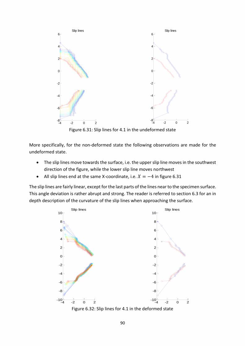
90
Figure 6.31: Slip lines for 4.1 in the undeformed state
More specifically, for the non-deformed state the following observations are made for the
undeformed state.
The slip lines move towards the surface, i.e. the upper slip line moves in the southwest
direction of the figure, while the lower slip line moves northwest
All slip lines end at the same X-coordinate, i.e. 𝑋 = −4 in figure 6.31
The slip lines are fairly linear, except for the last parts of the lines near to the specimen surface.
This angle deviation is rather abrupt and strong. The reader is referred to section 6.3 for an in
depth description of the curvature of the slip lines when approaching the surface.
Figure 6.32: Slip lines for 4.1 in the deformed state
-4 -2 0 2-8
-6
-4
-2
0
2
4
6Slip lines
-4 -2 0 2-8
-6
-4
-2
0
2
4
6Slip lines
-4 -2 0 2-10
-8
-6
-4
-2
0
2
4
6
8
10Slip lines
-4 -2 0 2-10
-8
-6
-4
-2
0
2
4
6
8
10Slip lines
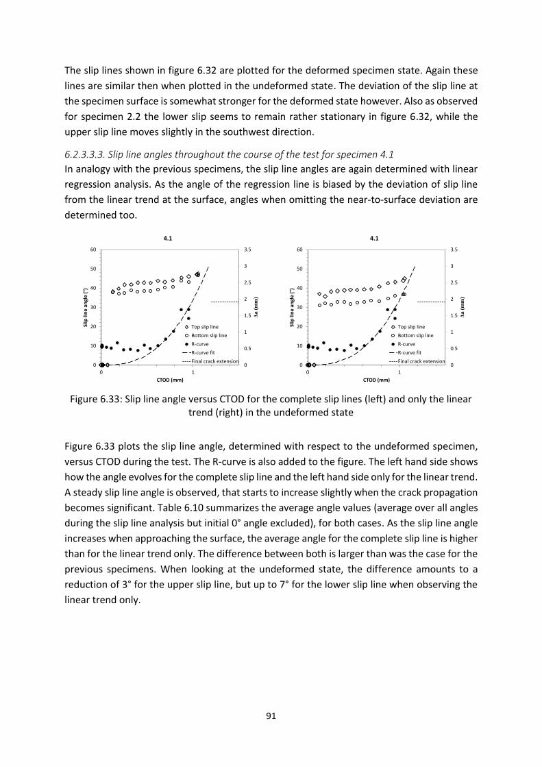
91
The slip lines shown in figure 6.32 are plotted for the deformed specimen state. Again these
lines are similar then when plotted in the undeformed state. The deviation of the slip line at
the specimen surface is somewhat stronger for the deformed state however. Also as observed
for specimen 2.2 the lower slip seems to remain rather stationary in figure 6.32, while the
upper slip line moves slightly in the southwest direction.
6.2.3.3.3. Slip line angles throughout the course of the test for specimen 4.1
In analogy with the previous specimens, the slip line angles are again determined with linear
regression analysis. As the angle of the regression line is biased by the deviation of slip line
from the linear trend at the surface, angles when omitting the near-to-surface deviation are
determined too.
Figure 6.33: Slip line angle versus CTOD for the complete slip lines (left) and only the linear
trend (right) in the undeformed state
Figure 6.33 plots the slip line angle, determined with respect to the undeformed specimen,
versus CTOD during the test. The R-curve is also added to the figure. The left hand side shows
how the angle evolves for the complete slip line and the left hand side only for the linear trend.
A steady slip line angle is observed, that starts to increase slightly when the crack propagation
becomes significant. Table 6.10 summarizes the average angle values (average over all angles
during the slip line analysis but initial 0° angle excluded), for both cases. As the slip line angle
increases when approaching the surface, the average angle for the complete slip line is higher
than for the linear trend only. The difference between both is larger than was the case for the
previous specimens. When looking at the undeformed state, the difference amounts to a
reduction of 3° for the upper slip line, but up to 7° for the lower slip line when observing the
linear trend only.
0
0.5
1
1.5
2
2.5
3
3.5
0
10
20
30
40
50
60
0 1
Δa (
mm
)
Slip
lin
e a
ngl
e (
°)
CTOD (mm)
4.1
Top slip line
Bottom slip line
R-curve
R-curve fit
Final crack extension0
0.5
1
1.5
2
2.5
3
3.5
0
10
20
30
40
50
60
0 1
Δa (
mm
)
Slip
lin
e a
ngl
e (
°)
CTOD (mm)
4.1
Top slip line
Bottom slip line
R-curve
R-curve fit
Final crack extension
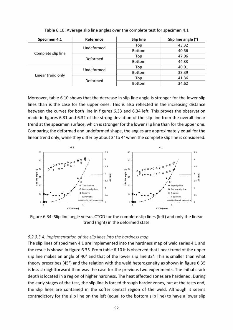
92
Table 6.10: Average slip line angles over the complete test for specimen 4.1
Specimen 4.1 Reference Slip line Slip line angle (°)
Complete slip line
Undeformed Top 43.32
Bottom 40.56
Deformed Top 47.06
Bottom 44.33
Linear trend only
Undeformed Top 40.01
Bottom 33.39
Deformed Top 41.36
Bottom 34.62
Moreover, table 6.10 shows that the decrease in slip line angle is stronger for the lower slip
lines than is the case for the upper ones. This is also reflected in the increasing distance
between the curves for both line in figures 6.33 and 6.34 left. This proves the observation
made in figures 6.31 and 6.32 of the strong deviation of the slip line from the overall linear
trend at the specimen surface, which is stronger for the lower slip line than for the upper one.
Comparing the deformed and undeformed shape, the angles are approximately equal for the
linear trend only, while they differ by about 3° to 4° when the complete slip line is considered.
Figure 6.34: Slip line angle versus CTOD for the complete slip lines (left) and only the linear
trend (right) in the deformed state
6.2.3.3.4. Implementation of the slip lines into the hardness map
The slip lines of specimen 4.1 are implemented into the hardness map of weld series 4.1 and
the result is shown in figure 6.35. From table 6.10 it is observed that linear trend of the upper
slip line makes an angle of 40° and that of the lower slip line 33°. This is smaller than what
theory prescribes (45°) and the relation with the weld heterogeneity as shown in figure 6.35
is less straightforward than was the case for the previous two experiments. The initial crack
depth is located in a region of higher hardness. The heat affected zones are hardened. During
the early stages of the test, the slip line is forced through harder zones, but at the tests end,
the slip lines are contained in the softer central region of the weld. Although it seems
contradictory for the slip line on the left (equal to the bottom slip line) to have a lower slip
0
0.5
1
1.5
2
2.5
3
3.5
0
10
20
30
40
50
60
0 1
Δa (
mm
)
Slip
lin
e a
ngl
e (
°)
CTOD (mm)
4.1
Top slip line
Bottom slip line
R-curve
R-curve fit
Final crack extension0
0.5
1
1.5
2
2.5
3
3.5
0
10
20
30
40
50
60
0 1
Δa (
mm
)
Slip
lin
e a
ngl
e (
°)
CTOD (mm)
4.1
Top slip line
Bottom slip line
R-curve
R-curve fit
Final crack extension
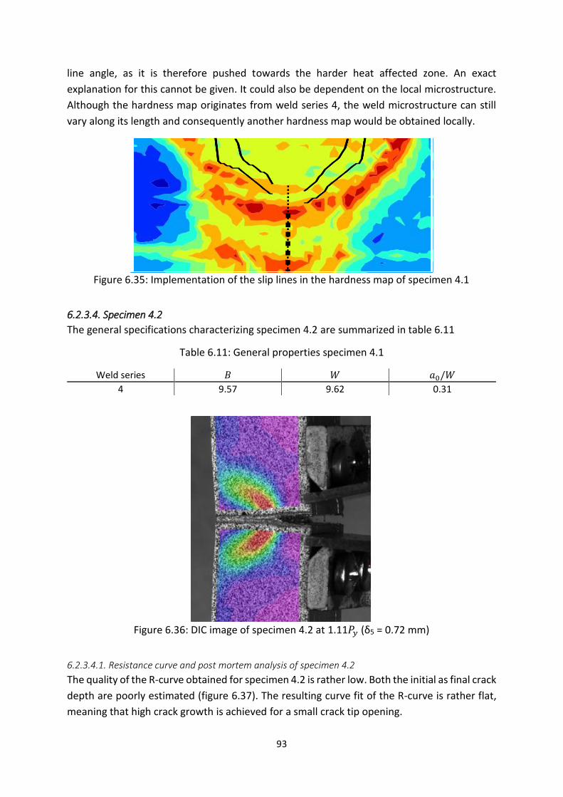
93
line angle, as it is therefore pushed towards the harder heat affected zone. An exact
explanation for this cannot be given. It could also be dependent on the local microstructure.
Although the hardness map originates from weld series 4, the weld microstructure can still
vary along its length and consequently another hardness map would be obtained locally.
Figure 6.35: Implementation of the slip lines in the hardness map of specimen 4.1
6.2.3.4. Specimen 4.2
The general specifications characterizing specimen 4.2 are summarized in table 6.11
Table 6.11: General properties specimen 4.1
Weld series 𝐵 𝑊 𝑎0/𝑊
4 9.57 9.62 0.31
Figure 6.36: DIC image of specimen 4.2 at 1.11𝑃𝑦 (δ5 = 0.72 mm)
6.2.3.4.1. Resistance curve and post mortem analysis of specimen 4.2
The quality of the R-curve obtained for specimen 4.2 is rather low. Both the initial as final crack
depth are poorly estimated (figure 6.37). The resulting curve fit of the R-curve is rather flat,
meaning that high crack growth is achieved for a small crack tip opening.
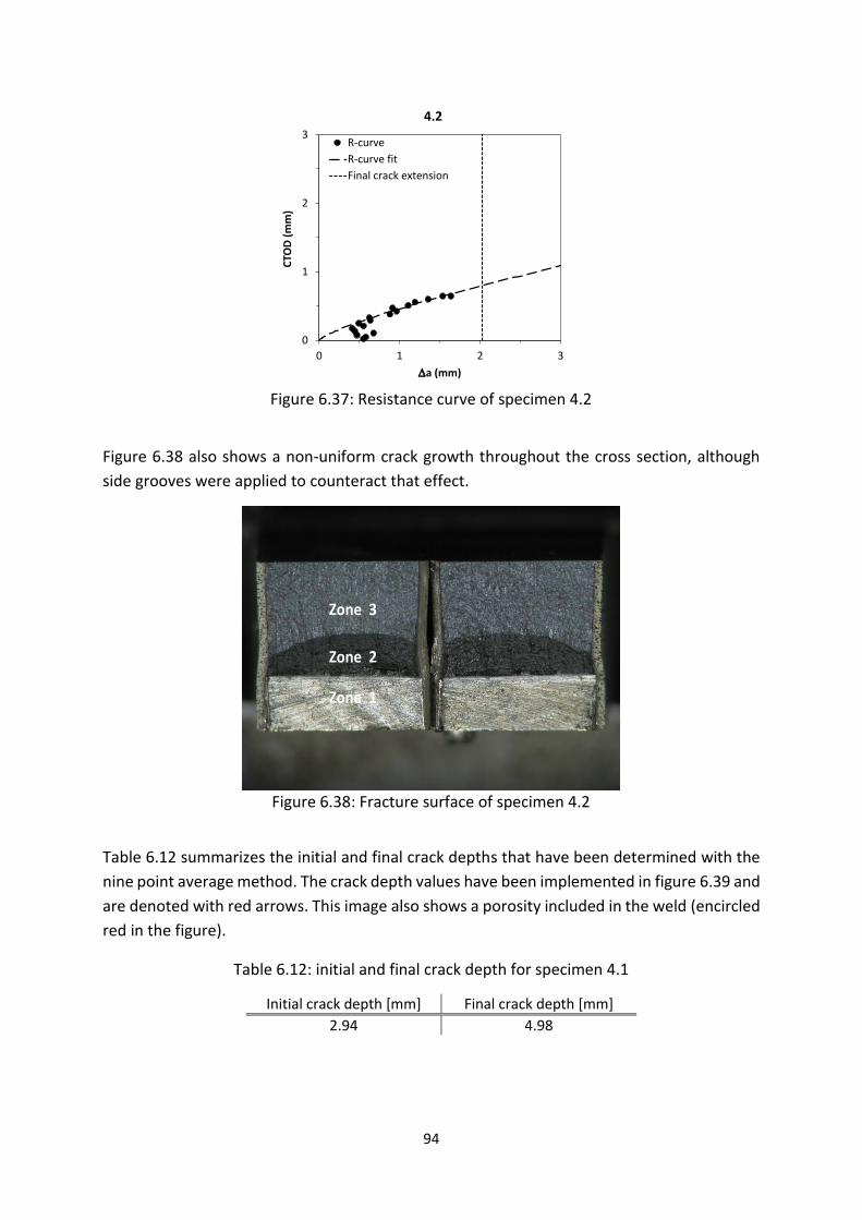
94
Figure 6.37: Resistance curve of specimen 4.2
Figure 6.38 also shows a non-uniform crack growth throughout the cross section, although
side grooves were applied to counteract that effect.
Figure 6.38: Fracture surface of specimen 4.2
Table 6.12 summarizes the initial and final crack depths that have been determined with the
nine point average method. The crack depth values have been implemented in figure 6.39 and
are denoted with red arrows. This image also shows a porosity included in the weld (encircled
red in the figure).
Table 6.12: initial and final crack depth for specimen 4.1
Initial crack depth [mm] Final crack depth [mm]
2.94 4.98
0
1
2
3
0 1 2 3
CTO
D (
mm
)
Da (mm)
4.2
R-curve
R-curve fit
Final crack extension
Zone 3
Zone 2
Zone 1

95
Figure 6.39: Post mortem microscopic photo of weld 4.2
6.2.3.4.2. Slip line trajectories in specimen 4.2
The slip line behaviour of specimen 4.2 is almost identical to that of 4.1. When comparing the
slip lines for both specimens no remarkable differences are observed. Only for specimen 4.2
in the undeformed state, the bending of the slip lines at the specimen surface is slightly less
as for specimen 4.1.
Figure 6.40: Slip lines for 4.2 in the non-deformed state
Final crack tip
Initial crack tip
-4 -2 0 2-10
-8
-6
-4
-2
0
2
4
6
8
10Slip lines
-4 -2 0 2-10
-8
-6
-4
-2
0
2
4
6
8
10Slip lines

96
Figure 6.41: Slip lines for 4.2 in the deformed state
6.2.3.4.3. Slip line angles throughout the course of the test for specimen 4.2
In last paragraph it was observed that the shape of the slip lines are almost identical with
those of specimen 4.1. This is also reflected in the evolution of the slip line angle. The larger
curvature of the slip lines of specimen 4.2 in the undeformed state resulted in an angle
increase of 1° to 2° (table 6.13). However, in the deformed state the angles are about 2° higher
for specimen 4.1.
Figure 6.42: Slip line angle versus CTOD for the complete slip lines (left) and only the linear
trend (right) in the non-deformed state
If only the linear trend is analyzed, i.e. excluding the knee at the specimen surface, the angles
for specimen 4.2 are about 2° higher for the upper slip line, but about 7° for the lower slip line.
Consequently, the angle difference for the linear trends of upper and lower slip line reduced
to about 3° for specimen 4.2 compared to specimen 4.1. Figures 6.42 and 6.43 indeed show
that the slip line angles for upper and lower slip line follow each other closely.
-4 -2 0 2-10
-8
-6
-4
-2
0
2
4
6
8
10Slip lines
-4 -2 0 2-10
-8
-6
-4
-2
0
2
4
6
8
10Slip lines
0
0.5
1
1.5
2
2.5
3
3.5
0
10
20
30
40
50
60
0 1
Δa (
mm
)
Slip
lin
e a
ngl
e (
°)
CTOD (mm)
4.2
Top slip line
Bottom slip line
R-curve
R-curve fit
Final crack extension0
0.5
1
1.5
2
2.5
3
3.5
0
10
20
30
40
50
60
0 1
Δa (
mm
)
Slip
lin
e a
ngl
e (
°)
CTOD (mm)
4.2
Top slip line
Bottom slip line
R-curve
R-curve fit
Final crack extension

97
Table 6.13: Average slip line angles over the complete test for specimen 4.2
Specimen 4.2 Reference Slip line Slip line angle (°)
Complete slip line
Undeformed Top 44.76
Bottom 42.32
Deformed Top 45.61
Bottom 42.86
Linear trend only
Undeformed Top 43.07
Bottom 40.68
Deformed Top 43.93
Bottom 40.93
The slip line angle evolution in figures 6.42 and 6.43 is similar to that observed for specimen
4.1. The angle increases slightly for increasing CTOD.
Figure 6.43: Slip line angle versus CTOD for the complete slip lines (left) and only the linear
trend (right) in the deformed state
6.2.3.4.4. Implementation of the slip lines into the hardness map
Figure 6.44 shows the implementation of the slip lines of specimen 4.2 into the hardness map
of weld series 4. The initial crack depth reaches into a harder zone in the weld center. The slip
lines are forced to start in this harder region. The conclusions are therefore similar to those
for specimen 4.1. At the right of figure 6.44, the slip lines can still avoid the harder heat
affected zone, while on the left hand side, the slip lines are forced through the harder heat
affected zone.
Figure 6.44: Implementation of the slip lines in the hardness map of specimen 4.2
0
0.5
1
1.5
2
2.5
3
3.5
0
10
20
30
40
50
60
0 1
Δa
(m
m)
Slip
lin
e a
ngl
e (
°)
CTOD (mm)
4.2
Top slip line
Bottom slip line
R-curve
R-curve fit
Final crack extension0
0.5
1
1.5
2
2.5
3
3.5
0
10
20
30
40
50
60
0 1
Δa
(m
m)
Slip
lin
e a
ngl
e (
°)
CTOD (mm)
4.2
Top slip line
Bottom slip line
R-curve
R-curve fit
Final crack extension

98
6.3. Numerical results This section presents the results for the simulations on homogeneous material that have been
introduced in chapter 5. For matter of analysis, the simulations are grouped according to their
geometry/boundary conditions, i.e. 2D plane strain, 2D plane stress, 3D (B = W) and 3D (B =
2W). From each group, the slip lines will be analyzed and trends are summarized. The section
ends by comparing these different results and coming up with general conclusions regarding
the numerical work.
First the convergence history of the simulations is discussed.
6.3.1. Overall convergence of the simulations
Here, the numerical simulations are executed by the finite element software until the final
displacement x, which is 4mm or L/x equal 50 for all simulations, is applied or if the time
increment becomes too small to allow for a converging analysis. The reason for non-
convergence can be of various kinds. Table 6.14 shows the convergence history of all
simulations that have been performed in the light of the parameter study. The simulations
that did not reach 50% completion are colored red. For the group B = W all simulations
converged, while for B = 2W only two did not converge, but nevertheless reached a significant
level of completion. Consequently, all simulation results of these two groups are used in
further analysis.
For the plane strain simulations however, some significant convergence problems are
observed for the E = 20000 GPa simulations. Most of them did not even meet 10% of full
completion. The Young’s modulus was chosen too extreme for these specific simulations to
converge. Also extreme values for the exponents of n, see n = 500, were disadvantageous for
convergence. This problem could probably be resolved by reducing the time steps used in
these simulations. However, the simulations were not repeated with smaller increment size
within the framework of this MSc thesis due to time restraints. Eventually, only the plane
strain simulations with E = 200 GPa are used in the next paragraphs.
The plane stress simulations mainly converged, except for extreme parameters E and n.
However, another problem was observed regarding the usability of the simulations for slip
line analysis. Figure 6.45 shows a snapshot of the specimen at the end of its simulation. The
plastic deformation is concentrated locally in the section of the crack. Hence, no slip line
patterns are observed at both sides of the crack. Also, the maximum plastic strains that occur
in the crack section are unrealistically high, with peak values exceeding 533.9% at the notch
tip. This was made possible as the simulations were executed with finite strain calculations,
i.e. taking second order effects into account for strain calculation. As such, neither the strain
patterns nor the obtained strain values turn out useful for further analysis.

99
Figure 6.45: Equivalent plastic strain in a plane stress simulation (n=20, E=200, a/W=03)
As was explained in chapter 3, the slip lines are evaluated at predefined instants in the
simulation history, dictated by the user through an increment interval. The slip lines are
extracted every 20 increments for all simulations. Consequently, the number of evaluations
varies for each simulation according to the total amount of increments that each simulation
executed. Generally, the amount of evaluations lies around 10 for each simulation.
6.3.2. Plane strain simulations
As the slip line theory derived by Hill (chapter 3) assumes plane strain conditions, the plane
strain simulations are discussed first. The theoretical solution for the slip lines in plane strain
conditions were determined at 45°. Here, the compliance with theory is checked by simulating
the plane strain specimens introduced in chapter 5 and this for various material properties
and crack depths.
This first section will provide an overview of the shape of the slip lines that are obtained for
the different simulations, while the next section will investigate the course of the slip lines in
more detail with the help of their slip line angles. Remind that only the simulations with E =
200 GPa are included in the discussion.
6.3.2.1. Slip line shape
Figure 6.46 shows the slip lines for the first (blue) and the last (red) slip line evaluation,
respectively corresponding with the start and end of the simulation. Please remark that both
upper and lower slip line are equal for each simulation as this is a logical result for a symmetric
specimen with uniform material properties.
Figure 6.46 displays the slip lines for four simulations in the deformed state, namely n = 10,
a0/W = 0.1 (top left); n = 15, a0/W = 0.3 (top right); n = 20, a0/W = 0.3 (bottom left); n = 500,
a0/W = 0.5 (bottom right). General conclusions are:
The slip line does not (n = 20 and 500 simulations), or only slightly (n = 10 and 15
simulations) deviate from its global trend when approaching the surface

100
The higher the Ramberg-Osgood exponent n and initial crack depth a0/W, the more
the slip line path at the end of the simulation deviates from its initial trajectory, i.e.
moving inwards
The start of the slip lines at the notch is more perpendicular to the notch with
increasing n
From the first observation, it can be concluded that the slip line deviation from the linear trend
is related to strain hardening of the material. The more the material can be strain hardened,
the more this effect of a deviating slip line towards the surface can present itself.
The slip line behaviour at the notch tip is less important regarding the overall slip line
evolution. At the notch tip, the plastic strains are unrealistically high. The mesh cells around
the notch have deformed severely (see figure 6.47), making the results coming from those
cells less reliable.
Figure 6.46: Slip lines for four configurations in the deformed state
-20 -15 -10 -5 0
-20
-15
-10
-5
0
5
10
15
Slip line paths during a SENT simulation
Specimen width [mm]
Specim
en length
[m
m]
Begin simulation
End simulation
-20 -15 -10 -5 0
-20
-15
-10
-5
0
5
10
15
Slip line paths during a SENT simulation
Specimen width [mm]
Specim
en length
[m
m]
Begin simulation
End simulation
-20 -15 -10 -5 0
-20
-15
-10
-5
0
5
10
15
Slip line paths during a SENT simulation
Specimen width [mm]
Specim
en length
[m
m]
Begin simulation
End simulation
-20 -15 -10 -5 0
-20
-15
-10
-5
0
5
10
15
Slip line paths during a SENT simulation
Specimen width [mm]
Specim
en length
[m
m]
Begin simulation
End simulation

Table 6.14: Overview of the convergence history of all simulations
Simulation Nr. 𝑛 𝐸 [𝐺𝑃𝑎] 𝑎0/𝑊 Percentage of simulation completed
Plane Strain Plane Stress 𝐵 = 𝑊 𝐵 = 2𝑊
1
10
200
0.1 100 100 100 100
2 0.3 100 100 100 100
3 0.5 100 100 100 100
4
20000
0.1 1.9 100 100 100
5 0.3 0.4 100 100 100
6 0.5 0.8 98.3 100 100
7
15
200
0.1 100 100 100 100
8 0.3 100 100 100 100
9 0.5 100 100 100 100
10
20000
0.1 0.8 100 100 100
11 0.3 7.9 99.3 100 100
12 0.5 1.6 84.4 100 100
13
20
200
0.1 43.6 100 100 100
14 0.3 100 100 100 100
15 0.5 100 100 100 100
16
20000
0.1 1.7 100 100 100
17 0.3 0.2 39.2 100 28.9
18 0.5 1.4 14.3 100 100
19
500
200
0.1 88.8 96 100 100
20 0.3 68.8 100 100 100
21 0.5 67.5 100 100 58.2
22
20000
0.1 0.23 7 100 100
23 0.3 0.3 56.5 100 100
24 0.5 1.8 3.1 100 100
10
1
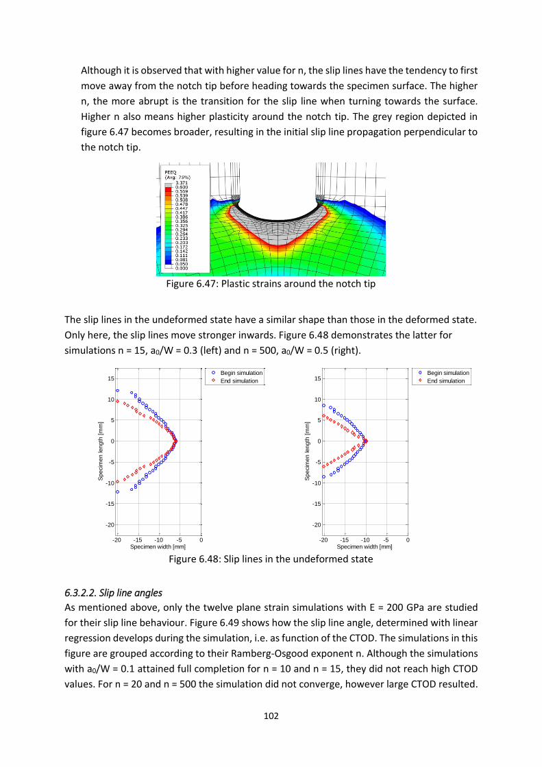
102
Although it is observed that with higher value for n, the slip lines have the tendency to first
move away from the notch tip before heading towards the specimen surface. The higher
n, the more abrupt is the transition for the slip line when turning towards the surface.
Higher n also means higher plasticity around the notch tip. The grey region depicted in
figure 6.47 becomes broader, resulting in the initial slip line propagation perpendicular to
the notch tip.
Figure 6.47: Plastic strains around the notch tip
The slip lines in the undeformed state have a similar shape than those in the deformed state.
Only here, the slip lines move stronger inwards. Figure 6.48 demonstrates the latter for
simulations n = 15, a0/W = 0.3 (left) and n = 500, a0/W = 0.5 (right).
Figure 6.48: Slip lines in the undeformed state
6.3.2.2. Slip line angles
As mentioned above, only the twelve plane strain simulations with E = 200 GPa are studied
for their slip line behaviour. Figure 6.49 shows how the slip line angle, determined with linear
regression develops during the simulation, i.e. as function of the CTOD. The simulations in this
figure are grouped according to their Ramberg-Osgood exponent n. Although the simulations
with a0/W = 0.1 attained full completion for n = 10 and n = 15, they did not reach high CTOD
values. For n = 20 and n = 500 the simulation did not converge, however large CTOD resulted.
-20 -15 -10 -5 0
-20
-15
-10
-5
0
5
10
15
Slip line paths during a SENT simulation
Specimen width [mm]
Specim
en length
[m
m]
Begin simulation
End simulation
-20 -15 -10 -5 0
-20
-15
-10
-5
0
5
10
15
Slip line paths during a SENT simulation
Specimen width [mm]
Specim
en length
[m
m]
Begin simulation
End simulation

103
Hence, non-converging simulations do not necessarily result in small final CTOD values. With
higher values for a0/W the slip lines are shorter and hence the applied displacement is
distributed over a shorter trajectory, resulting in higher strains and hence larger CTOD values.
However, if the exponent n becomes that large that the material behaves approximately
purely plastic, the CTOD can indeed become larger as shown in figure 6.49 for the simulation
a0/W = 0.1 and n = 500 because of the large plastic deformations that occur in the region of
the crack tip.
Figure 6.49: Slip line angle versus CTOD90 for the plane strain simulations in the
deformed state
An important observation is that the simulations with higher initial crack depth reached higher
slip line angles and that for all simulations, the slip line angle increases with increasing CTOD.
This increase in slip line angle can be quantified by plotting a linear regression line to the
curves in figure 6.49. The figure shows that the first angle of each simulation equals 0°,
referring to the undeformed shape and thus irrelevant regarding slip lines. In order not to bias
the result of the regression by these ‘zero degree’ slip line angle values, only the angles higher
than 40° are included in this regression analysis. The obtained regression lines are plotted in
figure 6.50. This figure summarizes all trends of increasing slip line angles of figure 6.49.
This figure shows that:
0 0.5 1 1.5 2 2.5 30
10
20
30
40
50
60
70
CTOD [mm]
Slip
line
ang
le [
°]
Slip line angle versus CTOD n=10
a/W = 0.1
a/W = 0.3
a/W = 0.5
0 0.5 1 1.5 2 2.5 30
10
20
30
40
50
60
70
CTOD [mm]
Slip
line
ang
le [
°]
Slip line angle versus CTOD n=15
a/W = 0.1
a/W = 0.3
a/W = 0.5
0 0.5 1 1.5 2 2.5 30
10
20
30
40
50
60
70
CTOD [mm]
Slip
line
ang
le [
°]
Slip line angle versus CTOD n=20
a/W = 0.1
a/W = 0.3
a/W = 0.5
0 0.5 1 1.5 2 2.5 30
10
20
30
40
50
60
70
CTOD [mm]
Slip
line
ang
le [
°]
Slip line angle versus CTOD n=500
a/W = 0.1
a/W = 0.3
a/W = 0.5
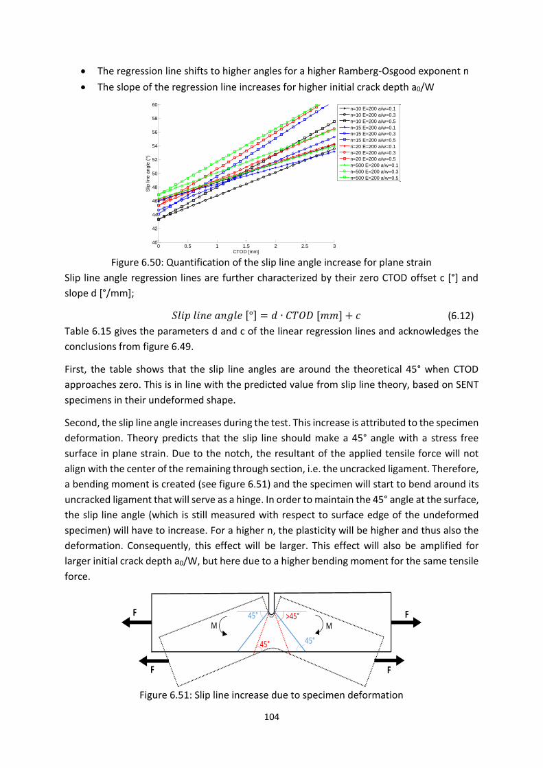
104
The regression line shifts to higher angles for a higher Ramberg-Osgood exponent n
The slope of the regression line increases for higher initial crack depth a0/W
Figure 6.50: Quantification of the slip line angle increase for plane strain
Slip line angle regression lines are further characterized by their zero CTOD offset c [°] and
slope d [°/mm];
𝑆𝑙𝑖𝑝 𝑙𝑖𝑛𝑒 𝑎𝑛𝑔𝑙𝑒 [°] = 𝑑 ∙ 𝐶𝑇𝑂𝐷 [𝑚𝑚] + 𝑐 (6.12)
Table 6.15 gives the parameters d and c of the linear regression lines and acknowledges the
conclusions from figure 6.49.
First, the table shows that the slip line angles are around the theoretical 45° when CTOD
approaches zero. This is in line with the predicted value from slip line theory, based on SENT
specimens in their undeformed shape.
Second, the slip line angle increases during the test. This increase is attributed to the specimen
deformation. Theory predicts that the slip line should make a 45° angle with a stress free
surface in plane strain. Due to the notch, the resultant of the applied tensile force will not
align with the center of the remaining through section, i.e. the uncracked ligament. Therefore,
a bending moment is created (see figure 6.51) and the specimen will start to bend around its
uncracked ligament that will serve as a hinge. In order to maintain the 45° angle at the surface,
the slip line angle (which is still measured with respect to surface edge of the undeformed
specimen) will have to increase. For a higher n, the plasticity will be higher and thus also the
deformation. Consequently, this effect will be larger. This effect will also be amplified for
larger initial crack depth a0/W, but here due to a higher bending moment for the same tensile
force.
Figure 6.51: Slip line increase due to specimen deformation
0 0.5 1 1.5 2 2.5 340
42
44
46
48
50
52
54
56
58
60
CTOD [mm]
Slip
lin
e a
ngle
(°)
Regression lines of the slip line angles for the slip lines
n=10 E=200 a/w=0.1
n=10 E=200 a/w=0.3
n=10 E=200 a/w=0.5
n=15 E=200 a/w=0.1
n=15 E=200 a/w=0.3
n=15 E=200 a/w=0.5
n=20 E=200 a/w=0.1
n=20 E=200 a/w=0.3
n=20 E=200 a/w=0.5
n=500 E=200 a/w=0.1
n=500 E=200 a/w=0.3
n=500 E=200 a/w=0.5
45°
F
F 45° >45°
45°
F
FMM

105
To summarize, the slip line angle complies with theory for the undeformed specimen and will
increase due to specimen bending around its uncracked ligament when a load is applied.
Table 6.15: Components of the regression lines with respect to the deformed specimen
𝑛 [-] 𝐸 [GPa] 𝑎0/𝑊 𝑐[°] 𝑑 [°/mm]
10
200
0.1 45.96 2.74
0.3 43.35 3.4
0.5 43.26 4.75
15
0.1 46.13 2.34
0.3 44.67 3.54
0.5 44.09 5.49
20
0.1 46.26 2.68
0.3 45.33 3.73
0.5 45.32 5.31
500
0.1 46.35 2.54
0.3 46.94 3.14
0.5 46.91 4.78
The analysis so far has been focusing on the determination of the slip lines with respect to the
deformed specimen. As already explained in chapter 3 and in section 6.1, the slip lines can
also be determined with respect to the initial shape of the specimen. In analogy with table
6.15, table 6.16 reports the results for the slip line angles with respect to the initial specimen
shape. Both the initial angles as well as the slopes of the angle increase during the test are
very close to the results of table 6.15. However, the stronger inward movement of the slip
lines in the undeformed state, observed in the previous section, is reflected in a slightly higher
regression slope d in table 6.16.
Table 6.16: Components of the regression lines with respect to the non-deformed specimen
𝑛 [-] 𝐸 [GPa] 𝑎0/𝑊 𝑐[°] 𝑑 [°/mm]
10
200
0.1 45.98 4.16
0.3 43.20 3.19
0.5 42.67 4.72
15
0.1 46.11 3.25
0.3 44.39 3.48
0.5 43.57 5.53
20
0.1 46.30 3.04
0.3 45.04 3.72
0.5 44.82 5.35
500
0.1 42.26 2.72
0.3 46.62 3.25
0.5 46.46 4.92
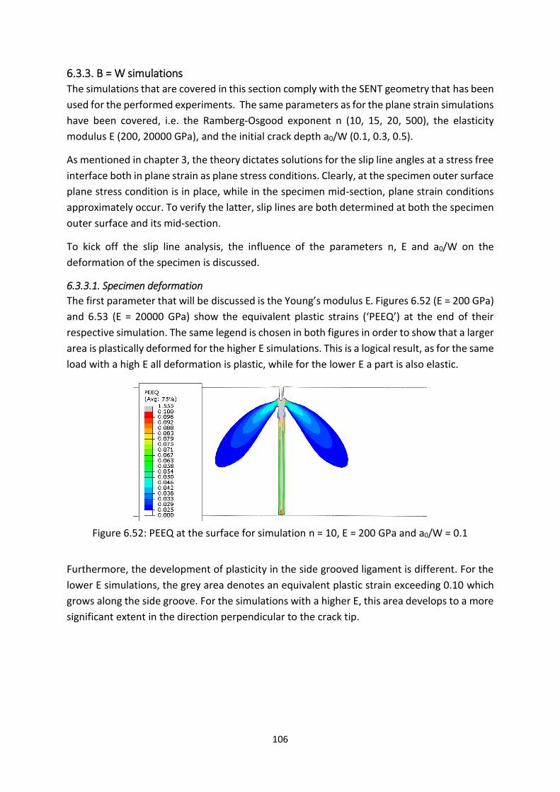
106
6.3.3. B = W simulations
The simulations that are covered in this section comply with the SENT geometry that has been
used for the performed experiments. The same parameters as for the plane strain simulations
have been covered, i.e. the Ramberg-Osgood exponent n (10, 15, 20, 500), the elasticity
modulus E (200, 20000 GPa), and the initial crack depth a0/W (0.1, 0.3, 0.5).
As mentioned in chapter 3, the theory dictates solutions for the slip line angles at a stress free
interface both in plane strain as plane stress conditions. Clearly, at the specimen outer surface
plane stress condition is in place, while in the specimen mid-section, plane strain conditions
approximately occur. To verify the latter, slip lines are both determined at both the specimen
outer surface and its mid-section.
To kick off the slip line analysis, the influence of the parameters n, E and a0/W on the
deformation of the specimen is discussed.
6.3.3.1. Specimen deformation
The first parameter that will be discussed is the Young’s modulus E. Figures 6.52 (E = 200 GPa)
and 6.53 (E = 20000 GPa) show the equivalent plastic strains (‘PEEQ’) at the end of their
respective simulation. The same legend is chosen in both figures in order to show that a larger
area is plastically deformed for the higher E simulations. This is a logical result, as for the same
load with a high E all deformation is plastic, while for the lower E a part is also elastic.
Figure 6.52: PEEQ at the surface for simulation n = 10, E = 200 GPa and a0/W = 0.1
Furthermore, the development of plasticity in the side grooved ligament is different. For the
lower E simulations, the grey area denotes an equivalent plastic strain exceeding 0.10 which
grows along the side groove. For the simulations with a higher E, this area develops to a more
significant extent in the direction perpendicular to the crack tip.

107
Figure 6.53: PEEQ at the surface for simulation n = 10, E = 20000 GPa and a0/W = 0.1
Another effect of the increase in elasticity modulus is shown in figures 6.54 (E = 200 GPa) and
6.55 (E = 20000 GPa). Both display a snapshot of their respective simulation when 47% of the
simulation is completed.
Figure 6.54: PEEQ at the surface for simulation n = 15, E = 200 GPa and a0/W = 0.5
The propagation of the plastic region differs in both figures. Whereas for low E the plastic
region grows in the side groove before the slip line regions develop, with high E modulus both
grow simultaneously. Consequently, the side groove region will have undergone higher plastic
deformation for low E, than in case of high E.
Figure 6.55: PEEQ at the surface for simulation n = 15, E = 20000 GPa and a0/W = 0.5

108
Next the effect of the parameter n is studied. Higher values of n imply a closer approximation
of perfect plasticity, i.e. less strain hardening of the material. As such for equal stresses, the
plastic strains are much higher for high n. This is also what is observed when looking at figures
6.56 and 6.57. The legends of both figures are equal for sake of comparison and for high value
of n the plastic strains are significantly higher than in the same region for the simulation with
lower n.
Figure 6.56: PEEQ at the surface for simulation n = 10, E = 200 GPa and a0/W = 0.3
Figure 6.57: PEEQ at the surface for simulation n = 500, E = 200 GPa and a0/W = 0.3
Finally, the notch tip behaviour is completely different at the mid-section. No side groove is
present in the mid-section, so the plastic regions grow with the slip lines and not in the through
section as is the case for the surface with side grooves. Figure 6.58 is a snapshot of the same
simulation and at the same instant as that of figure 6.54, but now showing the plasticity in the
mid-section. When comparing both figures, the effect of side grooves absence is clearly visible.

109
Figure 6.58: PEEQ at the mid-section for simulation n = 15, E = 200 GPa and a0/W = 0.5
6.3.3.2. Slip line shape
The course of the slip lines is discussed in this section. Figures 6.59 and 6.60 present the slip
lines at the specimen surface in the deformed state for a selected range of simulations out of
the total of 24 simulations with B = W: n = 10, E = 200 GPa, a0/W = 0.1 (top left); n = 10, E =
200 GPa, a0/W = 0.5 (top right); n = 10, E = 20000 GPa, a0/W = 0.1 (bottom left) and n = 10, E
= 20000 GPa, a0/W = 0.5 (bottom right). The blue (symbol: circle) graphs are the slip lines at
the beginning of the simulation, while the red (symbol: diamond) ones are those at the end of
the simulation.
Figure 6.59: Slip lines at the surface for four configurations in the deformed state
-20 -15 -10 -5 0
-20
-15
-10
-5
0
5
10
15
Slip line paths during a SENT simulation
Specimen width [mm]
Specim
en length
[m
m]
Begin simulation
End simulation
-20 -15 -10 -5 0
-20
-15
-10
-5
0
5
10
15
Slip line paths during a SENT simulation
Specimen width [mm]
Specim
en length
[m
m]
Begin simulation
End simulation
-20 -15 -10 -5 0
-20
-15
-10
-5
0
5
10
15
Slip line paths during a SENT simulation
Specimen width [mm]
Specim
en length
[m
m]
Begin simulation
End simulation
-20 -15 -10 -5 0
-20
-15
-10
-5
0
5
10
15
Slip line paths during a SENT simulation
Specimen width [mm]
Specim
en length
[m
m]
Begin simulation
End simulation

110
When studying the upper row of figure 6.59, which are the simulations with n = 10 and E =200
GPa and a0/W increasing from 0.1 (left) to 0.5 (right), the following observations can be made:
For low a0/W the slip lines are fairly linear but deviate from this trend when
approaching the surface edge
The slip lines move slightly inwards during the test
Higher a0/W results in higher crack tip opening which is translated in a larger distance
between the slip line starting points at the notch tip
These observations are confirmed when studying the upper row of figure 6.60, showing the
simulations n = 500, E = 200 GPa, a0/W = 0.1 (top left); n = 500, E = 200 GPa, a0/W = 0.5 (top
right); n = 20, E = 20000 GPa, a0/W = 0.1 (bottom left) and n = 20, E = 20000 GPa, a0/W = 0.5
(bottom right). However, the crack tip opening is larger here due to the larger plasticity at the
crack tip.
When comparing the figures in the lower row of figure 6.59, i.e. the simulations with E = 20000
GPa and a0/W increasing from 0.1 to 0.5, the following is noted:
For low a0/W, the slip line behaviour is equal to its counterpart with E = 200 GPa.
For increasing a0/W the slip lines move outwards and afterwards curve towards the
surface
The lower column of figure 6.60 learns that the effect of outwards moving slip lines is larger
for higher values of n.
Summarized, for realistic values for E (200 GPa), slip lines move inwards and curve when
approaching the surface. With higher values of E the slip lines initially move perpendicular to
notch direction before curving towards the surface.
-20 -15 -10 -5 0
-20
-15
-10
-5
0
5
10
15
Slip line paths during a SENT simulation
Specimen width [mm]
Specim
en length
[m
m]
Begin simulation
End simulation
-20 -15 -10 -5 0
-20
-15
-10
-5
0
5
10
15
Slip line paths during a SENT simulation
Specimen width [mm]
Specim
en length
[m
m]
Begin simulation
End simulation

111
Figure 6.60: Slip lines at the surface for four configurations in the deformed state
The effect of E on the slip line pattern can be explained when looking at the time history of
the simulations. Figures 6.54 and 6.55 of last section explained the different behaviour or the
plastic zone around the notch tip for both cases. With a normal E, the plastic zone grows along
the side groove before the slip lines develop themselves. Consequently, the slip lines can
develop freely. However, for a large value for E, the plastic zone grows perpendicular to the
original notch direction. The slip lines follow that direction initially before turning towards the
surface.
Now the question remains: Why do the slip lines curve when approaching the surface?
Different approaches are reasoned through to that respect.
The first approach is based on the theory that is outlined in chapter 3. From theory, a
theoretical solution for the slip line angle with a stress free surface in plane stress conditions
for rigid-perfectly plastic material is derived, namely 54.44°. The first approach verifies
whether the curvature could be related to theory. Polynomial regression was proven to be an
accurate tool to describe the slip line angle along the whole slip line, if an appropriate
polynomial degree is chosen. Therefore, polynomial regression will be used next. The material
from the simulations that complies best with the definition of plastic-perfectly rigid is that
with n = 500 and E = 20000 GPa. As the slip lines are symmetric for all simulations (symmetric
specimen and homogeneous material properties) only the upper slip line will be analyzed
further on. From chapter 3, it is learned that with polynomial regression (when analyzed for
the same X-values as the slip lines) a tangent to the regression line is drawn for each data
point. Consequently, for each data point, a regression angle results. However, the polynomial
regression analysis is very sensitive to the polynomial degree regarding the angles at the outer
edges. The optimal degree depends on the slip line shape, but when the latter is chosen
inappropriately, the angles for the outer points are false (see figure 6.61 right).
-20 -15 -10 -5 0
-20
-15
-10
-5
0
5
10
15
Slip line paths during a SENT simulation
Specimen width [mm]
Specim
en length
[m
m]
Begin simulation
End simulation
-20 -15 -10 -5 0
-20
-15
-10
-5
0
5
10
15
Slip line paths during a SENT simulation
Specimen width [mm]
Specim
en length
[m
m]
Begin simulation
End simulation

112
Figure 6.61: Polynomial regression (n = 2 right, n = 3 left) to determine slip line angle at
the surface for simulation n = 500, E = 20000 GPa and a0/W = 0.1
Table 6.17 reports the angles for the point at the surface edge and up to five points removed
from that edge. As such the surface edge region is covered completely.
Table 6.17: Polynomial regression slip line angles
Polynomial degree
Slip line Slip line angle at # points from the surface edge[°]
At edge -1 -2 -3 -4 -5
2 Start 80.82 66.44 63.69 61.10 60.96 58.52
End 77.92 63.50 60.77 58.21 58.05 55.67
3 Start 89.78 67.11 63.45 60.23 60.06 57.24
End 99.19 64.86 60.05 56.12 55.89 52.74
From figure 6.61 and table 6.17 it is noticed that the polynomial degree two is best describing
the slip line angle at the surface. Furthermore, the angle at the surface amounts to about 80°.
This angle is much larger than the theoretical 54.44°. Therefore it is concluded that this
assumption is not solely explaining the slip line curvature when approaching the surface.
The second approach explains the behaviour based on local strain hardening of the material.
From figure 6.62 it is observed that when the slip lines are developed, two plastic zones are
created at the surface edge. The plastic deformation in this zone will strain harden the material
locally and could influence the slip line pattern.
Figure 6.62: Local strain hardening of the material at the surface edge
-20 -15 -10 -5 00
2
4
6
8
10
12
14
16
18
specimen width [mm]
specim
en length
[m
m]
Polynomial regression of the upper slip lines (degree: 2)
slip line start
slip line end
regression line start
regression line end
-20 -15 -10 -5 00
2
4
6
8
10
12
14
16
18
specimen width [mm]
specim
en length
[m
m]
Polynomial regression of the upper slip lines (degree: 2)
slip line start
slip line end
regression line start
regression line end

113
However as the curvature is also present in the early stages of the simulations when there is
little plastic deformation yet and also simulations with n = 500 (i.e. very little strain hardening)
undergo this effect, the assumption, when indeed influencing the slip line pattern, cannot be
the only reason for the slip line deviation towards the surface. Therefore, a third and final
approach is described next.
The third approach explains the bending of the slip lines through the bending moment that is
applied onto the uncracked ligament due to the misalignment between the applied force and
the center of the uncracked ligament (see figure 6.63). The resulting lever arm (‘r’ in figure
6.63) of the load with respect to the centerline of the uncracked ligament creates the bending
moment (M). A notched specimen that is loaded in bending has a completely different slip line
pattern, as shown in figure 3.3. The theory of slip lines in a SENB specimen relates the slip line
evolution to the stresses in the uncracked ligament. When a bending moment is applied as in
figure 6.63, the upper half of the uncracked ligament experiences a tensile force, while the
lower half is compressed (blue arrows in figure 6.63). This change in stress state explains the
curving slip line. However as for SENT specimens, both a tensile force (red arrows), uniformly
distributed over the cross section and the additional bending moment occur. The resulting
stress state (green arrows) is as drawn in figure 6.63. From the theory of SENB, it is concluded
that the moment the stress state in the uncracked ligament changes sign, the slip lines will
start to move inwards as shown in figure 6.63.
For the slip lines under consideration here, the bending moment is not large enough to
compensate the tensile stress, i.e. to reach a point of sign change in stresses. However, the
bending moment is large enough to cause the slip line to curve when approaching the surface,
as slip line curvature is related here to a decreasing resulting stress in the uncracked ligament.
So it is concluded that the value of the bending moment determines slip line curvature.
Figure 6.63: SENT: a combination of tensile force and bending moment
The third approach is inherent to the SENT test and therefore is applicable to all simulations
under consideration, hence also the simulations in which rigid-perfectly plastic material is
considered. This explanation is therefore considered as the most valid one.
The discussion so far, focused on the slip lines at the specimen surface, i.e. plane stress
conditions. As mentioned in the introduction of this section, slip lines are also evaluated at
the specimen’s mid-section. The goal is to verify if the slip lines behave differently when plane
strain condition is approximated. Figure 6.64, shows the slip lines for n = 20, E = 200 GPa and
d
Centerline uncracked ligament
FF
MM
Slip line
r

114
a0/W = 0.1 with plane strain (left), at the specimen surface of B = W (middle) and at the
specimen mid-section of B = W (right). Generally, the difference between the slip lines at the
surface and mid-section are small, as also observed with the example in figure 6.64. Therefore,
the same conclusions can be made as for the slip lines at the surface. However differences are
small, the results for the mid-section lie in between the plane strain and the surface slip lines.
Namely, from figure 6.64 it is observed that for higher n the slip lines at the mid-section are
straighter with respect to the surface edge than for slip lines at the specimen surface. This
straight behaviour at the specimen surface was also observed with the plane strain
simulations, as displayed in figure 6.64 left.
Figure 6.64: Slip lines for n= 20, E=200 GPa and a0/W = 0.1
The discussion of the slip lines in the undeformed state is analog to that for plane strain. The
dependencies of the slip line behaviour on the parameters is equal to that for the deformed
state, however, the inward movement is stronger for all simulations in the undeformed state.
This means that for the simulations with E = 200 GPa, the total inward movement is larger,
while for those with E = 20000 GPa, the outward movement is largely compensated. Figure
6.65 displays the slip lines in the undeformed state for simulatinos n = 10, E = 200 GPa and
a0/W = 0.1 (left); n = 20, E = 20000 GPa and a0/W = 0.5 (middle) and n = 500, E = 200 GPa and
a0/W = 0.5 (right), which can be compared with their respective deformed counterparts in
figures 6.59 and 6.60.
Figure 6.65: Slip lines in the undeformed state
-20 -15 -10 -5 0
-20
-15
-10
-5
0
5
10
15
Slip line paths during a SENT simulation
Specimen width [mm]
Specim
en length
[m
m]
Begin simulation
End simulation
-20 -15 -10 -5 0
-20
-15
-10
-5
0
5
10
15
Slip line paths during a SENT simulation
Specimen width [mm]
Specim
en length
[m
m]
Begin simulation
End simulation
-20 -15 -10 -5 0
-20
-15
-10
-5
0
5
10
15
Slip line paths during a SENT simulation
Specimen width [mm]
Specim
en length
[m
m]
Begin simulation
End simulation
-20 -15 -10 -5 0
-15
-10
-5
0
5
10
15
Slip line paths during a SENT simulation
Specimen width [mm]
Specim
en length
[m
m]
Begin simulation
End simulation
-20 -15 -10 -5 0
-15
-10
-5
0
5
10
15
Slip line paths during a SENT simulation
Specimen width [mm]
Specim
en length
[m
m]
Begin simulation
End simulation
-20 -15 -10 -5 0
-15
-10
-5
0
5
10
15
Slip line paths during a SENT simulation
Specimen width [mm]
Specim
en length
[m
m]
Begin simulation
End simulation
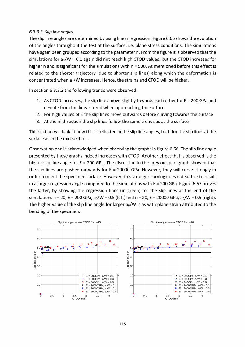
115
6.3.3.3. Slip line angles
The slip line angles are determined by using linear regression. Figure 6.66 shows the evolution
of the angles throughout the test at the surface, i.e. plane stress conditions. The simulations
have again been grouped according to the parameter n. From the figure it is observed that the
simulations for a0/W = 0.1 again did not reach high CTOD values, but the CTOD increases for
higher n and is significant for the simulations with n = 500. As mentioned before this effect is
related to the shorter trajectory (due to shorter slip lines) along which the deformation is
concentrated when a0/W increases. Hence, the strains and CTOD will be higher.
In section 6.3.3.2 the following trends were observed:
1. As CTOD increases, the slip lines move slightly towards each other for E = 200 GPa and
deviate from the linear trend when approaching the surface
2. For high values of E the slip lines move outwards before curving towards the surface
3. At the mid-section the slip lines follow the same trends as at the surface
This section will look at how this is reflected in the slip line angles, both for the slip lines at the
surface as in the mid-section.
Observation one is acknowledged when observing the graphs in figure 6.66. The slip line angle
presented by these graphs indeed increases with CTOD. Another effect that is observed is the
higher slip line angle for E = 200 GPa. The discussion in the previous paragraph showed that
the slip lines are pushed outwards for E = 20000 GPa. However, they will curve strongly in
order to meet the specimen surface. However, this stronger curving does not suffice to result
in a larger regression angle compared to the simulations with E = 200 GPa. Figure 6.67 proves
the latter, by showing the regression lines (in green) for the slip lines at the end of the
simulations n = 20, E = 200 GPa, a0/W = 0.5 (left) and n = 20, E = 20000 GPa, a0/W = 0.5 (right).
The higher value of the slip line angle for larger a0/W is as with plane strain attributed to the
bending of the specimen.
0 0.5 1 1.5 2 2.5 3
0
10
20
30
40
50
60
70
CTOD [mm]
Slip
line a
ngle
[°]
Slip line angle versus CTOD for n=15
E = 200GPa, a/W = 0.1
E = 200GPa, a/W = 0.3
E = 200GPa, a/W = 0.5
E = 20000GPa, a/W = 0.1
E = 20000GPa, a/W = 0.3
E = 20000GPa, a/W = 0.5
0 0.5 1 1.5 2 2.5 30
10
20
30
40
50
60
70
CTOD [mm]
Slip
line a
ngle
[°]
Slip line angle versus CTOD for n=20
E = 200GPa, a/W = 0.1
E = 200GPa, a/W = 0.3
E = 200GPa, a/W = 0.5
E = 20000GPa, a/W = 0.1
E = 20000GPa, a/W = 0.3
E = 20000GPa, a/W = 0.5

116
Figure 6.66: Slip line angles at the surface versus CTOD90 for the B = W simulations
(deformed)
Table 6.18 summarizes the results of the linear regression lines that have been applied to the
graphs in 6.66, in analogy with the analysis for plane strain. The table confirms the rising angle
with CTOD and shows lower slopes for the E = 20000 GPa simulations. The initial slip line angle
varies between 45° and 50° and the slopes at the mid-section are lower when E = 200 GPa and
higher when E = 20000 GPa compared to those at the surface.
Figure 6.67: Influence of the inwards and outwards slip line movement regression slope
When comparing the values for the specimen surface and the mid-section, it is noted that
both the offset and the slope d do not differ significantly for the surface and the mid-section.
This observation complies with the one made in section 6.3.3.2, reporting only small
differences for the slip lines at the mid-section and surface.
0 0.5 1 1.5 2 2.5 30
10
20
30
40
50
60
70
CTOD [mm]
Slip
line a
ngle
[°]
Slip line angle versus CTOD for n=20
E = 200GPa, a/W = 0.1
E = 200GPa, a/W = 0.3
E = 200GPa, a/W = 0.5
E = 20000GPa, a/W = 0.1
E = 20000GPa, a/W = 0.3
E = 20000GPa, a/W = 0.5
0 0.5 1 1.5 2 2.5 30
10
20
30
40
50
60
70
CTOD [mm]
Slip
line a
ngle
[°]
Slip line angle versus CTOD for n=500
E = 200GPa, a/W = 0.1
E = 200GPa, a/W = 0.3
E = 200GPa, a/W = 0.5
E = 20000GPa, a/W = 0.1
E = 20000GPa, a/W = 0.3
E = 20000GPa, a/W = 0.5
-20 -15 -10 -5
-15
-10
-5
0
5
10
15
Slip line paths during a SENT simulation
Specimen width [mm]
Speci
men le
ngth
[m
m]
Begin simulation
End simulation
-20 -15 -10 -5
-15
-10
-5
0
5
10
15
Slip line paths during a SENT simulation
Specimen width [mm]
Spec
imen
lengt
h [
mm
]
Begin simulation
End simulation

117
Table 6.18: Components of the regression lines (deformed)
Surface Mid-section 𝑛 (-) 𝐸 [GPa] 𝑎0/𝑊 𝑐 (°) 𝑑 (°/mm) 𝑐 (°) 𝑑 (°/mm)
10
200
0.1 47.14 12.61 47.51 9.75
0.3 44.45 3.25 45.57 3.25
0.5 44.28 4.35 44.41 3.85
15
0.1 48.56 6.86 48.74 6.27
0.3 45.95 2.98 47.43 2.72
0.5 46.58 3.89 46.54 3.21
20
0.1 49.24 4.66 49.70 3.10
0.3 46.82 2.78 48.61 2.26
0.5 47.46 3.58 46.71 3.12
500
0.1 51.89 1.01 52.31 1.14
0.3 49.87 1.66 50.17 1.59
0.5 49.69 2.82 48.77 2.49
10
20000
0.1 48.85 3.74 49.83 5.58
0.3 46.61 1.08 48.00 1.17
0.5 48.86 0.84 48.08 1.41
15
0.1 49.49 2.95 50.63 5.66
0.3 47.81 1.22 49.57 1.03
0.5 50.84 0.96 49.86 0.38
20
0.1 48.93 6.07 50.50 5.65
0.3 48.62 1.24 49.91 1.30
0.5 51.40 0.93 50.90 1.03
500
0.1 52.35 -2.11 54.12 -3.35
0.3 50.99 0.89 52.04 1.16
0.5 52.45 1.48 51.67 1.51
The trends noticed in figure 6.66 and table 6.18 are structured more closely next.
Figure 6.68 shows the evolution of the slip line angle with CTOD in case of varying n. The slopes
of these lines are equal, except for n = 500 for which it is slightly lower and the slip line angle
at simulation start increases for increasing n. The angle at simulation start is 45° for n = 10 and
increases to 50° for n = 500.
Figure 6.68: Slip line evolution versus CTOD for varying Ramberg-Osgood exponent n
0 0.5 1 1.5 2 2.5 340
42
44
46
48
50
52
54
56
58
60
CTOD [mm]
Slip
lin
e a
ngle
(°)
n=10 E=200 a/w=0.3
n=15 E=200 a/w=0.3
n=20 E=200 a/w=0.3
n=500 E=200 a/w=0.3

118
The influence of the Young’s modulus on the slip line angle evolution is shown in figure 6.69.
The angle increase is higher in case of a smaller value for E. The angles for the graphs with E =
200 GPa are also shifted parallel towards higher angles with respect to their E = 20000 GPa
counterpart. The slip line angles at the start of the simulation vary between 46° and 49°.
Figure 6.69: Slip line evolution versus CTOD for varying Ramberg-Osgood exponent 𝑛 and
Young’s modulus E The observations made in figure 6.69 can be reasoned as follows. For an E = 200 GPa, it was
shown earlier that the plastic deformation was highly concentrated along the side groove. This
section is indeed weaker due to its smaller cross section and hence higher stresses result. Due
to the strong plastic deformation, the section along the side grooves will act as a hinge and
promote bending of the specimen halves around that hinge (see figures 6.52 and 6.53). This
leads to an increase in the slip line angle that is higher than for the E = 20000 GPa simulations
as the deformation along the side grooves is less for these simulations and thus the hinge
principle is less intense.
The influence of the initial crack depth is shown in figure 6.70. From the graphs in figure 6.66
it could already be observed that the simulations with a0/W = 0.1 do not reach high CTOD
values. With a0/W that low, the rest ligament is still amounting to 90% of the specimen width.
The stress concentration in the side groove region is lower and consequently also the plastic
deformation. Also the region of high plasticity around the notch tip is smaller, reflecting in a
crack that is less severely opened. Consequently, lower values of maximum CTOD are
obtained.
Figure 6.70: Slip line evolution versus CTOD for initial crack depth a0/W
0 0.5 1 1.5 2 2.5 340
42
44
46
48
50
52
54
56
58
60
CTOD [mm]
Slip
lin
e a
ngle
(°)
n=15 E=200 a/w=0.3
n=15 E=20000 a/w=0.3
n=20 E=200 a/w=0.3
n=20 E=20000 a/w=0.3
0 0.5 1 1.5 2 2.5 340
42
44
46
48
50
52
54
56
58
60
CTOD [mm]
Slip
lin
e a
ngle
(°)
n=20 E=200 a/w=0.1
n=20 E=200 a/w=0.3
n=20 E=200 a/w=0.5
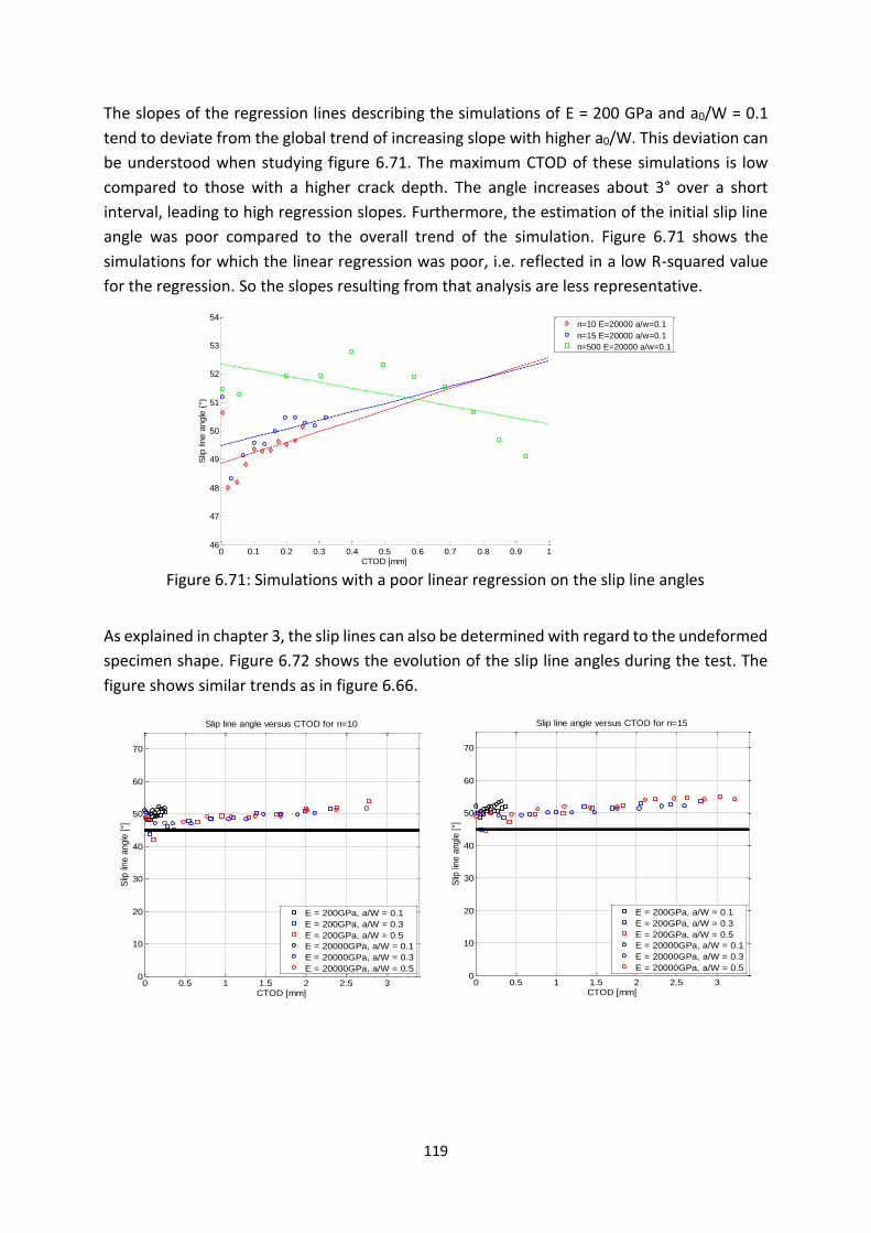
119
The slopes of the regression lines describing the simulations of E = 200 GPa and a0/W = 0.1
tend to deviate from the global trend of increasing slope with higher a0/W. This deviation can
be understood when studying figure 6.71. The maximum CTOD of these simulations is low
compared to those with a higher crack depth. The angle increases about 3° over a short
interval, leading to high regression slopes. Furthermore, the estimation of the initial slip line
angle was poor compared to the overall trend of the simulation. Figure 6.71 shows the
simulations for which the linear regression was poor, i.e. reflected in a low R-squared value
for the regression. So the slopes resulting from that analysis are less representative.
Figure 6.71: Simulations with a poor linear regression on the slip line angles
As explained in chapter 3, the slip lines can also be determined with regard to the undeformed
specimen shape. Figure 6.72 shows the evolution of the slip line angles during the test. The
figure shows similar trends as in figure 6.66.
0 0.1 0.2 0.3 0.4 0.5 0.6 0.7 0.8 0.9 146
47
48
49
50
51
52
53
54
CTOD [mm]
Slip
lin
e a
ngle
(°)
n=10 E=20000 a/w=0.1
n=15 E=20000 a/w=0.1
n=500 E=20000 a/w=0.1
0 0.5 1 1.5 2 2.5 30
10
20
30
40
50
60
70
CTOD [mm]
Slip
line a
ngle
[°]
Slip line angle versus CTOD for n=10
E = 200GPa, a/W = 0.1
E = 200GPa, a/W = 0.3
E = 200GPa, a/W = 0.5
E = 20000GPa, a/W = 0.1
E = 20000GPa, a/W = 0.3
E = 20000GPa, a/W = 0.5
0 0.5 1 1.5 2 2.5 30
10
20
30
40
50
60
70
CTOD [mm]
Slip
line a
ngle
[°]
Slip line angle versus CTOD for n=15
E = 200GPa, a/W = 0.1
E = 200GPa, a/W = 0.3
E = 200GPa, a/W = 0.5
E = 20000GPa, a/W = 0.1
E = 20000GPa, a/W = 0.3
E = 20000GPa, a/W = 0.5

120
Figure 6.72: Slip line angles at the mid-section versus CTOD90 for the B = W simulations
(undeformed)
In table 6.19, the regression line slope and offset are summarized for regression analysis of
figure 6.72. When comparing table 6.18 with table 6.19, i.e. the slip lines in the deformed state
with the undeformed state it is observed that the offset c does not differ remarkable. This is
indeed logical as at the start of the simulation, no difference exists between the deformed
and undeformed state.
Table 6.19: Components of the regression lines (undeformed)
Surface Mid-section 𝑛 (-) 𝐸 [GPa] 𝑎0/𝑊 𝑐 (°) 𝑑 (°/mm) 𝑐 (°) 𝑑 (°/mm)
10
200
0.1 47.14 14.55 47.52 12.37
0.3 44.26 2.88 45.37 2.94
0.5 43.78 3.78 43.78 3.78
15
0.1 48.54 8.31 48.72 8.37
0.3 45.70 2.74 47.12 2.62
0.5 46.03 3.50 45.87 3.40
20
0.1 49.18 5.97 49.63 5.09
0.3 46.54 2.62 48.24 2.29
0.5 46.89 3.26 46.02 3.42
500
0.1 51.55 2.59 51.95 3.37
0.3 49.48 1.72 49.68 1.90
0.5 49.14 2.58 48.04 2.95
10
20000
0.1 48.80 6.81 49.78 8.89
0.3 46.38 0.92 47.77 1.04
0.5 48.57 0.63 47.82 1.39
15
0.1 49.40 5.68 50.55 8.57
0.3 47.56 1.21 49.33 1.06
0.5 50.55 1.06 49.65 1.68
20
0.1 48.79 8.81 50.37 8.61
0.3 48.37 1.34 49.67 1.44
0.5 51.15 1.14 50.74 1.47
500
0.1 52.00 1.26 53.77 0.33
0.3 50.87 1.19 51.95 1.53
0.5 52.27 1.83 51.60 2.15
0 0.5 1 1.5 2 2.5 30
10
20
30
40
50
60
70
CTOD [mm]
Slip
line a
ngle
[°]
Slip line angle versus CTOD for n=20
E = 200GPa, a/W = 0.1
E = 200GPa, a/W = 0.3
E = 200GPa, a/W = 0.5
E = 20000GPa, a/W = 0.1
E = 20000GPa, a/W = 0.3
E = 20000GPa, a/W = 0.5
0 0.5 1 1.5 2 2.5 30
10
20
30
40
50
60
70
CTOD [mm]
Slip
line a
ngle
[°]
Slip line angle versus CTOD for n=500
E = 200GPa, a/W = 0.1
E = 200GPa, a/W = 0.3
E = 200GPa, a/W = 0.5
E = 20000GPa, a/W = 0.1
E = 20000GPa, a/W = 0.3
E = 20000GPa, a/W = 0.5

121
Furthermore, the slopes d in the undeformed state are generally higher than for the deformed
state. Figure 6.73 demonstrates the latter for simulation n = 20 E = 200 GPa and a0/W = 0.3.
Figure 6.73: Slip lines in the deformed state (left) versus undeformed state (right)
6.3.4. B = 2W simulations
The simulations discussed in this section have a cross section that is twice as large as that in
the previous section. Again slip lines are extracted both at the specimen surface and in the
mid-section. However, as the mid-section is now surrounded by twice as much material, plane
strain conditions should be better approximated in that section.
The results for these simulations closely approximate those of the B = W simulations.
Therefore, this section is briefer in the discussion of the results. For an in depth explanation
of the observed trend, the reader is referred to section 6.3.3.
6.3.4.1. Specimen deformation
The influence of the parameters on the strain fields in the specimen is analog to that discussed
in section 6.3.3.1. The side grooves implemented in the B = 2W specimens have the same
depth as those implemented in the B = W simulations, i.e. 1 mm. Therefore, the B = 2W
through section at the location of the side grooves is relatively stronger than that of the B =
W specimen. The strain concentration along that section will consequently be smaller as can
be observed when comparing figure 6.74 with figure 6.56.
Figure 6.74: PEEQ at the surface for simulation n = 10, E = 200 and a0/W = 0.3
-20 -15 -10 -5 0
-20
-15
-10
-5
0
5
10
15
Slip line paths during a SENT simulation
Specimen width [mm]
Specim
en length
[m
m]
Begin simulation
End simulation
-20 -15 -10 -5 0
-20
-15
-10
-5
0
5
10
15
Slip line paths during a SENT simulation
Specimen width [mm]
Specim
en length
[m
m]
Begin simulation
End simulation

122
6.3.4.2. Slip line shape
First the slip lines at the specimen surface, i.e. planes tress conditions are presented in figure
6.75 and figure 6.76. The slip lines shown in those figures have the same parameters as in
figures 6.59 and 6.60, i.e. n = 10, E = 200 GPa, a0/W = 0.1 (top left); n = 10, E = 200 GPa, a0/W
= 0.5 (top right); n = 10, E = 20000 GPa, a0/W = 0.1 (bottom left) and n = 10, E = 20000 GPa,
a0/W = 0.5 (bottom right) for figure 6.75, while for figure 6.76 those are n = 500, E = 200 GPa,
a0/W = 0.1 (top left); n = 500, E = 200 GPa, a0/W = 0.5 (top right); n = 20, E = 20000 GPa, a0/W
= 0.1 (bottom left) and n = 20, E = 20000 GPa, a0/W = 0.5 (bottom right).
Figure 6.75: Slip lines at the surface for four configurations in the deformed state
Comparing figures 6.59 and 6.75, it is clear that the results are fairly similar. For E = 200 GPa,
no differences are observed. Only for E = 20000 GPa, it is noticed that the slip lines remain
stationary for a0/W = 0.1 instead of moving slightly inwards. From figures 6.60 and 6.76 it is
also noted that this stationary behaviour of the slip lines for E = 20000 GPa is persisting when
n increases. Furthermore, the crack tip opening is less identifiable with increasing n (compare
top right of both figures), which was the case for the B = W simulations. As can be understood
from this paragraph, the differences at the surface are particularly small. The small differences
that are observed are attributed to the discussion of figure 6.74. The side groove is relatively
-20 -15 -10 -5 0
-20
-15
-10
-5
0
5
10
15
Slip line paths during a SENT simulation
Specimen width [mm]
Specim
en length
[m
m]
Begin simulation
End simulation
-20 -15 -10 -5 0
-20
-15
-10
-5
0
5
10
15
Slip line paths during a SENT simulation
Specimen width [mm]
Specim
en length
[m
m]
Begin simulation
End simulation
-20 -15 -10 -5 0
-20
-15
-10
-5
0
5
10
15
Slip line paths during a SENT simulation
Specimen width [mm]
Specim
en length
[m
m]
Begin simulation
End simulation
-20 -15 -10 -5 0
-20
-15
-10
-5
0
5
10
15
Slip line paths during a SENT simulation
Specimen width [mm]
Specim
en length
[m
m]
Begin simulation
End simulation

123
seen not as deep as for the B = W. Consequently, the plastic deformation in the groove is less
strong. The discussion of B = W introduced the concept of hinge working around the uncracked
ligament (especially due to plasticity concentration in the side groove). As this effect is smaller
for the B = 2W simulations, the rather stationary behaviour of the simulations with low a0/W
is explained as the bending moment is the smallest for small a0/W.
Figure 6.76: Slip lines at the surface for four configurations in the deformed state
The slip lines at the mid-section do not differ from those of the specimen B = W when taking
the annotations of last paragraph in account. Just as with the B = W simulations, their
evolution lies between the results for plane strain and those at the specimen surface. This is
once more illustrated with figure 6.77.
-20 -15 -10 -5 0
-20
-15
-10
-5
0
5
10
15
Slip line paths during a SENT simulation
Specimen width [mm]
Specim
en length
[m
m]
Begin simulation
End simulation
-20 -15 -10 -5 0
-20
-15
-10
-5
0
5
10
15
Slip line paths during a SENT simulation
Specimen width [mm]
Specim
en length
[m
m]
Begin simulation
End simulation
-20 -15 -10 -5 0
-20
-15
-10
-5
0
5
10
15
Slip line paths during a SENT simulation
Specimen width [mm]
Specim
en length
[m
m]
Begin simulation
End simulation
-20 -15 -10 -5 0
-20
-15
-10
-5
0
5
10
15
Slip line paths during a SENT simulation
Specimen width [mm]
Specim
en length
[m
m]
Begin simulation
End simulation

124
Figure 6.77: Slip lines for n= 500, E=200 GPa and a0/W = 0.3
6.3.4.3. Slip line angles
As the slip line shape is not significantly different from the B = W simulations, the slip line
angles will follow the same trends as discussed for B = W. The slip line angles versus CTOD in
the deformed state are drawn in figure 6.69. Clearly, the discussion of figure 6.66 could be
repeated. While the starting angles, i.e. offset c, again range from 45° to 50°, the slopes d are
slightly lower. This can both be observed in figure 6.78 as in table 6.20. This indeed
acknowledges the observation in the previous section of the more stationary slip line pattern.
As initial and final slip line approximately overlap in most cases, the angle increase is lower
too.
-20 -15 -10 -5 0
-20
-15
-10
-5
0
5
10
15
Slip line paths during a SENT simulation
Specimen width [mm]
Specim
en length
[m
m]
Begin simulation
End simulation
-20 -15 -10 -5 0
-20
-15
-10
-5
0
5
10
15
Slip line paths during a SENT simulation
Specimen width [mm]
Specim
en length
[m
m]
Begin simulation
End simulation
-20 -15 -10 -5 0
-20
-15
-10
-5
0
5
10
15
Slip line paths during a SENT simulation
Specimen width [mm]
Specim
en length
[m
m]
Begin simulation
End simulation
0 0.5 1 1.5 2 2.5 30
10
20
30
40
50
60
70
CTOD [mm]
Slip
lin
e a
ngle
[°]
Slip line angle versus CTOD for n=10
E = 200GPa, a/W = 0.1
E = 200GPa, a/W = 0.3
E = 200GPa, a/W = 0.5
E = 20000GPa, a/W = 0.1
E = 20000GPa, a/W = 0.3
E = 20000GPa, a/W = 0.5
0 0.5 1 1.5 2 2.5 30
10
20
30
40
50
60
70
CTOD [mm]
Slip
line a
ngle
[°]
Slip line angle versus CTOD for n=15
E = 200GPa, a/W = 0.1
E = 200GPa, a/W = 0.3
E = 200GPa, a/W = 0.5
E = 20000GPa, a/W = 0.1
E = 20000GPa, a/W = 0.3
E = 20000GPa, a/W = 0.5

125
Figure 6.78: Slip line angles at the surface versus CTOD90 for the B = 2W simulations
(deformed)
Table 6.20: Components of the regression lines (deformed)
Surface Mid-section 𝑛 (-) 𝐸 [GPa] 𝑎/𝑊 𝑐 (°) 𝑑 (°/mm) 𝑐 (°) 𝑑 (°/mm)
10
200
0.1 47.28 13.36 45.56 1.57
0.3 43.67 38.62 43.26 25.08
0.5 45.00 3.93 44.39 3.07
15
0.1 48.34 7.79 45.62 5.06
0.3 46.14 2.45 44.94 2.07
0.5 46.53 3.36 46.36 2.64
20
0.1 49.05 4.48 46.07 3.15
0.3 46.68 2.25 45.90 1.68
0.5 47.83 2.93 46.71 2.79
500
0.1 50.84 0.28 48.20 -0.62
0.3 49.16 1.40 48.34 0.75
0.5 50.43 1.59 48.00 2.77
10
20000
0.1 48.10 -0.03 45.14 0.89
0.3 46.64 0.10 45.13 0.83
0.5 47.96 0.31 46.54 0.53
15
0.1 48.68 -2.44 45.94 8.91
0.3 47.13 0.12 46.51 0.48
0.5 49.38 0.45 47.92 0.56
20
0.1 48.77 -1.40 46.31 7.41
0.3 48.84 -2.11 47.27 -0.82
0.5 49.37 1.14 48.52 0.31
500
0.1 50.20 -4.62 48.76 -1.47
0.3 48.62 0.73 48.20 0.59
0.5 50.55 1.34 49.93 1.18
Just as with the B = W simulations, some linear regression lines did not correlate the data well.
This is either caused by a poor estimation of the first slip line angle, or due to a very nervous
trajectory of the slip line angle versus CTOD. Figure 6.79 shows examples of simulations that
0 0.5 1 1.5 2 2.5 30
10
20
30
40
50
60
70
CTOD [mm]
Slip
line a
ngle
[°]
Slip line angle versus CTOD for n=20
E = 200GPa, a/W = 0.1
E = 200GPa, a/W = 0.3
E = 200GPa, a/W = 0.5
E = 20000GPa, a/W = 0.1
E = 20000GPa, a/W = 0.3
E = 20000GPa, a/W = 0.5
0 0.5 1 1.5 2 2.5 30
10
20
30
40
50
60
70
CTOD [mm]
Slip
line a
ngle
[°]
Slip line angle versus CTOD for n=500
E = 200GPa, a/W = 0.1
E = 200GPa, a/W = 0.3
E = 200GPa, a/W = 0.5
E = 20000GPa, a/W = 0.1
E = 20000GPa, a/W = 0.3
E = 20000GPa, a/W = 0.5

126
had a poor correlation of the regression analysis and clearly it is noted that they have data
points varying largely over a short CTOD distance.
Figure 6.79: Simulations with a poor linear regression on the slip line angles
The very large slope of simulation n = 10, E = 200 GPa and a0/W=0.3, as reported in table 6.20,
is even so explained with this observation. As the simulations with a0/W = 0.1 reach much
lower CTOD values in general, they are more sensitive to this phenomenon. Hence, the
resulting regression lines do not resemble the real variation well in those cases.
The slip line angles have also been determined for the undeformed state. Their evolution with
increasing CTOD has been visualized in figure 6.80, while table 6.21 summarizes the results of
the regression analysis. The difference between the undeformed state of the B = W
simulations and B = 2W simulations is also very small. Just as for the B = W simulations, the
slopes d of the regression analysis are higher than for the deformed state, while the offset c
remains equal to that of the deformed case (see table 6.21). Compared to the rather stationary
evolution for the deformed state, from figure 6.80 it is noted that the slip line angles for the
undeformed state increase with CTOD, as it was the case for the specimen B = W.
0 0.1 0.2 0.3 0.4 0.5 0.6 0.7 0.8 0.9 140
42
44
46
48
50
52
CTOD [mm]
Slip
lin
e a
ngle
[°]
n = 10 E = 200GPa, a/W = 0.3
n = 20 E = 20000GPa, a/W = 0.1
n = 500 E = 200GPa, a/W = 0.1
0 0.5 1 1.5 2 2.5 30
10
20
30
40
50
60
70
CTOD [mm]
Slip
line a
ngle
[°]
Slip line angle versus CTOD for n=10
E = 200GPa, a/W = 0.1
E = 200GPa, a/W = 0.3
E = 200GPa, a/W = 0.5
E = 20000GPa, a/W = 0.1
E = 20000GPa, a/W = 0.3
E = 20000GPa, a/W = 0.5
0 0.5 1 1.5 2 2.5 30
10
20
30
40
50
60
70
CTOD [mm]
Slip
line a
ngle
[°]
Slip line angle versus CTOD for n=15
E = 200GPa, a/W = 0.1
E = 200GPa, a/W = 0.3
E = 200GPa, a/W = 0.5
E = 20000GPa, a/W = 0.1
E = 20000GPa, a/W = 0.3
E = 20000GPa, a/W = 0.5

127
Figure 6.80: Slip line angles at the mid-section versus CTOD90 for the B = 2W simulations
(undeformed)
Table 6.21 also indicates that the plane strain condition is better approximated at the mid-
section of B = 2W. Compared to the results for B = W, the offset value c is even closer to
the theoretical 45°.
Table 6.21: Components of the regression lines (undeformed)
Surface Mid-section 𝑛 (-) 𝐸 [GPa] 𝑎/𝑊 𝑐 (°) 𝑑 (°/mm) 𝑐 (°) 𝑑 (°/mm)
10
200
0.1 47.29 15.86 45.57 4.92
0.3 43.58 33.72 43.14 22.89
0.5 44.54 3.15 43.86 2.78
15
0.1 48.33 9.70 45.60 7.92
0.3 45.95 2.04 44.76 1.94
0.5 46.05 2.73 45.80 2.54
20
0.1 49.03 6.13 46.02 5.81
0.3 46.47 1.91 45.68 1.64
0.5 47.33 2.38 46.12 2.82
500
0.1 50.59 1.95 47.93 2.30
0.3 48.83 1.22 47.95 0.97
0.5 49.88 1.17 47.36 2.98
10
20000
0.1 48.07 0.23 45.12 1.19
0.3 46.49 -0.17 45.00 0.73
0.5 47.70 -0.23 46.34 0.23
15
0.1 48.61 0.86 45.88 12.67
0.3 47.64 -0.07 46.36 0.45
0.5 49.18 0.13 47.76 0.57
20
0.1 48.68 1.73 46.23 11.04
0.3 48.82 -2.64 47.27 -1.16
0.5 49.18 0.97 48.39 0.47
500
0.1 49.94 -1.08 48.54 2.70
0.3 48.49 0.78 48.10 0.88
0.5 50.38 1.49 49.89 1.72
0 0.5 1 1.5 2 2.5 30
10
20
30
40
50
60
70
CTOD [mm]
Slip
line a
ngle
[°]
Slip line angle versus CTOD for n=20
E = 200GPa, a/W = 0.1
E = 200GPa, a/W = 0.3
E = 200GPa, a/W = 0.5
E = 20000GPa, a/W = 0.1
E = 20000GPa, a/W = 0.3
E = 20000GPa, a/W = 0.5
0 0.5 1 1.5 2 2.5 30
10
20
30
40
50
60
70
CTOD [mm]
Slip
lin
e a
ngle
[°]
Slip line angle versus CTOD for n=500
E = 200GPa, a/W = 0.1
E = 200GPa, a/W = 0.3
E = 200GPa, a/W = 0.5
E = 20000GPa, a/W = 0.1
E = 20000GPa, a/W = 0.3
E = 20000GPa, a/W = 0.5
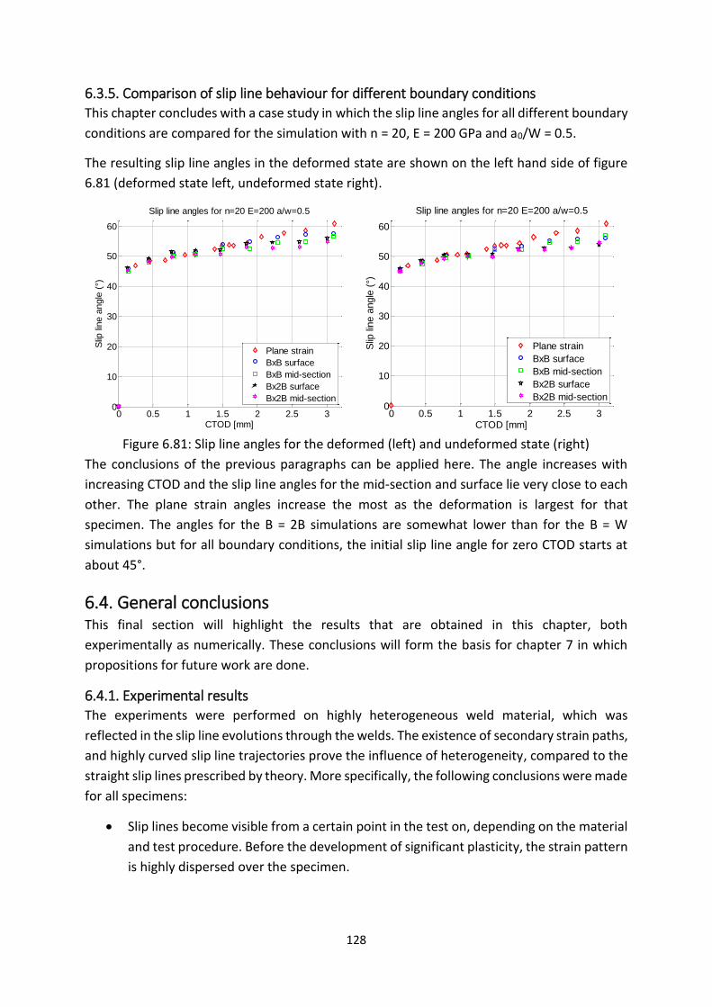
128
6.3.5. Comparison of slip line behaviour for different boundary conditions This chapter concludes with a case study in which the slip line angles for all different boundary
conditions are compared for the simulation with n = 20, E = 200 GPa and a0/W = 0.5.
The resulting slip line angles in the deformed state are shown on the left hand side of figure
6.81 (deformed state left, undeformed state right).
Figure 6.81: Slip line angles for the deformed (left) and undeformed state (right)
The conclusions of the previous paragraphs can be applied here. The angle increases with
increasing CTOD and the slip line angles for the mid-section and surface lie very close to each
other. The plane strain angles increase the most as the deformation is largest for that
specimen. The angles for the B = 2B simulations are somewhat lower than for the B = W
simulations but for all boundary conditions, the initial slip line angle for zero CTOD starts at
about 45°.
6.4. General conclusions This final section will highlight the results that are obtained in this chapter, both
experimentally as numerically. These conclusions will form the basis for chapter 7 in which
propositions for future work are done.
6.4.1. Experimental results
The experiments were performed on highly heterogeneous weld material, which was
reflected in the slip line evolutions through the welds. The existence of secondary strain paths,
and highly curved slip line trajectories prove the influence of heterogeneity, compared to the
straight slip lines prescribed by theory. More specifically, the following conclusions were made
for all specimens:
Slip lines become visible from a certain point in the test on, depending on the material
and test procedure. Before the development of significant plasticity, the strain pattern
is highly dispersed over the specimen.
0 0.5 1 1.5 2 2.5 30
10
20
30
40
50
60
CTOD [mm]
Slip
lin
e a
ngle
(°)
Slip line angles for n=20 E=200 a/w=0.5
Plane strain
BxB surface
BxB mid-section
Bx2B surface
Bx2B mid-section
0 0.5 1 1.5 2 2.5 30
10
20
30
40
50
60
CTOD [mm]
Slip
lin
e a
ngle
(°)
Slip line angles for n=20 E=200 a/w=0.5
Plane strain
BxB surface
BxB mid-section
Bx2B surface
Bx2B mid-section

129
Deformed state
Slip lines move inwards upon the occurrence of crack growth
From the notch tip onwards, the slip lines start linear but can undergo a specific
trajectory depending on the weld heterogeneity.
The slip lines deviate from the global trend when approaching the specimen surface.
Undeformed state
The upper and lower slip line move towards the surface and this translation is related
to the crack growth
The slip lines can additionally move inwards, i.e. the slip line angle increases
The slip line angle increase during the test is not unanimously related to the crack growth
during the test. Specimen 2.2 did not show this angle increase, while for the other specimens
the point of starting crack growth and angle increase could not exactly be linked due to the
poor correspondence between δ5 and CTOD90.
The slip line angles during the test depend strongly on the exact trajectory of the slip lines and
thus the heterogeneity. Both stable slip line angles as increasing angles have been observed.
The slip line angles in the undeformed state are lower than for the deformed state. This is
contradictory with the numerical results. Whether the angles in the undeformed or deformed
state are larger could be related to the amount of localized bending around the uncracked
ligament versus the amount of elongation of the specimen. This effect needs to be studied
more in detail in future work.
6.4.2. Numerical results The results of the numerical simulations are summarized next. All simulations have been
performed on homogeneous material with varying parameters and geometries (n = 10, 15, 20,
500; E = 200, 20000 GPa; a0/W = 0.1, 0.3, 0.5). The plane stress simulations did not turn out
useful for slip line analysis due to strong necking in the section of the notch.
6.4.2.1. Plane strain simulations
The simulations with E = 20000 GPa did not converge (less than 10 % completion) and are
therefore not considered.
Regarding the slip line shape, the following was observed:
The slip lines are linear
Slip lines deviate only slightly (n = 10, 15) or even negligibly (n = 20, 500) from this
linear trend when approaching the surface. From this it is assumed that strain
hardening has an influence on the slip line curvature at the surface edge
The slip lines start more in the perpendicular direction with respect to the notch for
increasing n. This observation is related to the higher plastic deformation at the notch
tip.

130
With increasing a0/W and n, the slip lines move inwards. This is related to bending of
the specimen around the uncracked ligament.
The slip line shape in the undeformed state is similar, but the slip lines move stronger
inwards.
These observations are reflected in the course of the slip line angle, determined with linear
regression, during the simulation.
Slip line length decreases with increasing a0/W, resulting in higher CTOD values as a
function of applied deformation
The slip line angles increase with CTOD for all simulations, due to the specimen
deformation. The bending moment is stronger for higher a0/W and the deformation
increases with n.
o The slip line angles versus CTOD shift to higher angles with higher n
o The angle increase is stronger for higher a0/W
The slip line angles at the start of the simulation (CTOD = 0) lie around 45°, both for
the deformed and undeformed state
A stronger increase in slip line angle is observed for the undeformed state
6.4.2.2. B = W simulations
Slip lines have been evaluated both at the specimen outer surface and in the mid-section, in
the deformed and undeformed state.
The slip line shape was observed to be dependent on the parameters and locus of evaluation:
E = 200 GPa and for all n:
o For low initial crack depth a0/W the slip lines are linear, but deviate from this
trend when approaching the surface edge
o Slip lines move slightly inwards for all a0/W
o The starting points of the slip lines at the notch move apart during the
simulation. This effect is more pronounced for higher n.
E = 20000 GPa and for all n:
o The behaviour at low a0/W is equal to the slip lines for E = 200 GPa.
o With higher a0/W, the slip lines move outwards and curve to the surface
afterwards. The latter is stronger for higher n.
The slip lines in the undeformed state move stronger inwards
To explain the curvature of the slip lines at the surface edge, three theories have been
proposed. The first explains the phenomenon based on the theoretical boundary condition of
slip lines in plane stress at a stress free surface. The second approach assumes strain
hardening at the edge to be the cause, while the third approach starts from the theory of SENB
and relates the curvature to a changing stress state in the uncracked ligament.
The behaviour of the slip lines at the mid-section is very close to that at the surface, but
tending to the slip lines in plane strain.

131
The trends noticed with studying the slip line shape are also translated into the slip line angles.
The slip line angle increases for higher CTOD, i.e. inwards moving slip lines. This effect
is smaller for higher E, where the angle tends to stabilize for higher CTOD.
The initial angles lie between 45° and 50°, increasing with n.
The slip line angle evolution depends an n, E and a0/W:
o The angle increases for higher n
o The increase is smaller for lower E
o The increase is larger with higher a0/W
For the undeformed state, the same dependencies occur, with the initial angles equal
to the deformed state, but the angle increase is generally higher.
6.4.2.3. B = 2W simulations
The conclusions for the B = 2W simulations are equal to the B = W simulations, as only the
following slight differences are observed:
The slip lines are more stationary for E = 20000 GPa and small a0/W. This is reflected
in a smaller angle increase versus CTOD
The mid-section better approximates plane strain conditions, as the initial angles are
closer to the theoretical 45°

132
Chapter 7
Conclusions and future work 7.1. Conclusions The study of slip lines in weld failure analysis promises to be a useful tool in achieving
improved homogenization models. However, there is a significant gap between the theoretical
concepts and experimental / numerical observations. Numerous factors influence the slip lines
in the specimen and these are not taken into account in the theoretical derivations. This work
serves as a basis in understanding the slip line behaviour in relation to weld heterogeneity,
geometric and material properties in the context of SENT testing.
This master thesis started with the establishment of algorithms for the extraction of slip lines
from SENT experiments analyzed with digital image correlation (DIC) and simulations with the
finite element software ABAQUS®. The agreement of both approaches has been verified for
plain base material and at the same time, the influence of side grooves on the slip line
evolution has been studied. It was observed that plastic deformation is largely concentrated
along these side grooves and consequently affects the slip line behaviour.
In total 96 simulations were performed to study the effect of material properties and loading/
boundary conditions on the slip lines in a SENT specimen. From these simulations it was
concluded that the assumed 45° angle assumed in the UGent weld homogenization model
holds for the main part of the slip line trajectory if the specimen is not deformed yet. The angle
increases during the course of the test, which is plausibly related to the specimen deformation
and more specifically to the localized bending of the specimen around its uncracked ligament.
This effect is strengthened with increasing initial crack depth a0/W.
SENT experiments have been executed for three different weld series to observe the slip line
behaviour in a highly heterogeneous weld environment. From those tests, it is observed that
the theoretical and numerical results for homogeneous material can be a strong simplification
of the true slip line evolution. Weld heterogeneity can cause the slip lines to adopt complex
shapes, strongly deviating from the linear shape, but also secondary slip line paths are
observed. Consequently, the deviation from the theoretical 45° angle assumed in weld
homogenization can be more significant for heterogeneous welds than was the case for the
simulations with homogeneous material.
As this research is far from done, some propositions for further research are reported in the
next section.

133
7.2. Future work This master thesis showed the influence of weld heterogeneity on slip line behaviour.
Moreover, simulations acknowledged the influence of material properties and loading
conditions. Those material properties were chosen to study the influence of realistic material
properties on the slip line pattern, compared to the non-realistic material property
assumptions in theory. As such the experimental and numerical work has been performed
rather independently.
The next step of the slip line research at Soete Laboratory could be to encompass the
following:
1. The agreement of the experimental and simulation results have currently only been
verified for plain base material. The next step would be to compare both approaches
for a heterogeneous weld. If the conformity holds for complex weld compositions,
simulations can form the basis for fast and accurate slip line studies for a larger number
of different welds.
2. As only four experiments have provided valuable results regarding the slip line study,
a large number of SENT experiments could be performed on a widespread variety of
welds. These welds can be selected according to strength and strength distribution.
The study could focus on the sensitivity of slip lines to strength variations in the weld.
From the experiments performed in this study, it is observed that regions with higher
hardness are avoided if possible. However, quantifying this effect should be the next
step in the relation of weld heterogeneity and slip line evolution.
3. From all experiments and simulations, it appeared that the slip lines behave differently
when approaching the surface. Three different approaches have been proposed to
describe that effect. However, hard proof was not found yet. With the homogenization
model, the overall trend of the slip lines are searched for. Although, its explanation
could be important to fully understand the slip line evolution in the weld.
4. The slip lines positions change when considering them in the deformed or undeformed
specimen state. The resulting slip line angles of the deformed shape were observed to
be larger than for the undeformed state, while the opposite was noted with the
simulations. The difference was proposed to be depending on the degree of local
bending of the specimen around the uncracked ligament versus specimen elongation.
However, this assumption needs to be verified.

134
Bibliography
[1] Verstraete M., “Experimental-Numerical Evaluation of Ductile Tearing Resistance and Tensile Strain Capacity of Biaxially Loaded Pipelines”, Ph.D. thesis, Ghent University, 2014.
[2] Det Norske Veritas, “DNV-RP-F108. Fracture Control for Pipeline Installation Methods Introducing Cyclic Plastic Strain”, January, 2006.
[3] Van Minnebruggen K. and Van Puyvelde D., “Experimentele evaluatie van plastische vervormingen en scheurgroei in gelaste constructies”, MsC thesis, Ghent University, 2011.
[4] Nyhus B., Polanco M.L., and Orjasaether O., “SENT Specimens an alternative to SENB Specimens”, 22nd International Conference on Offshore Mechanicsand Arctic engineering, Cancun, Mexico, 2003.
[5] Van Minnebruggen K., Van Puyvelde D., De Waele W., Verstraete M., Hertelé S., and Denys R., “Implementation of an Unloading Compliance Procedure for Measurement of Crack Growth in Pipeline Steel”, Sustainable Construction and Design, 2011.
[6] Verstraete M., Denys R., Van Minnebruggen K., Hertelé S., and De Waele W., “Determination of CTOD resistance curves in side-grooved Single-Edge Notched Tensile specimens using full field deformation measurements”, Engineering Fracture Mechanics, vol. 110, pp. 12–22, September 2013.
[7] Rice J.R., “A Path Independent Integral and the Approximate Analysis of Strain Concentration by Notches and Cracks”, Journal of Applied Mechanics, vol. 35, pp. 379–386, 1968.
[8] Hertelé S., De Waele W., Verstraete M., Denys R., and O’Dowd N., “J-integral analysis of heterogeneous mismatched girth welds in clamped single-edge notched tension specimens”, International Journal of Pressure Vessels and Piping, vol. 119, pp. 95–107, July 2014.
[9] Kumar V., German M.D., and Shih C.F., “An engineering approach for elastic-plastic fracture analysis EPRI”, topical report N° 1237-1, July 1981.
[10] Rice J.R. and Rosengren G.F., “Plane Strain Deformation near a Crack Tip in a Power-Law Hardening Material”, Journal of the Mechanics and Physics of Solids, vol. 16, pp. 1–12, 1968.
[11] Hutchinson J.W., “Singular Behaviour at the End of a Tensile Crack in a Hardening Material”, Journal of the Mechanics and Physics of Solids, vol. 16, pp. 13–31, 1968.
[12] Zhu X.K., Jang S.K., and Chen Y.F., “A Modification of J-Q Theory and its Applications,” International Journal of Fracture, pp. 47–52, 2001.
[13] O’Dowd N. and Shih C.F., “Family of crack-tip fields characterized by a triaxiality parameter- I. Structure of fields”, Journal of the Mechanics and Physics of Solids, vol. 39, no. 8, pp. 989–1015, 1991.

135
[14] Schwalbe K., Heerens J., Zerbst U., Pisarski H.G. and Koçak M., "EFAM GTP 02 - the GKSS Test Procedure for Determining the Fracture Behaviour of Materials", GKSS-Forschungszentrum Geesthacht GmbH, Geesthacht, 2002.
[15] Verstraete M., De Waele W., Denys R., and Van Minnebruggen K., “Measurement of Ductile Crack Extension in Single Edge Notch Tensile Specimens”, 15th International Conference on Experimental Mechanics, pp. 1–11, 2012.
[16] Verstraete M., Hertelé S., Denys R., Van Minnebruggen K., and De Waele W., “Evaluation and interpretation of ductile crack extension in SENT specimens using unloading compliance technique”, Engineering Fracture Mechanics, vol. 115, pp. 190–203, January 2014.
[17] Milne I., Ainsworth R.A., Dowling A.R., Stewart A.T., “R6 Assessment of the integrity of structures containing defects”, International Journal of Pressure Vessels and Piping, vol. 32, pp. 9-104, 1988.
[18] British Standard Institute,“British Standard 7910 Guide on Methods for Assessing of Flaw in Fusion Welded Structures”, p. 7910, 1999.
[19] Chiesa M., Nyhus B., Skallerus B., and Thaulow C., “Efficient Fracture Assessment of Pipelines . A Constraint-Corrected SENT Specimen Approach”, Engineering Fracture Mechanics, vol. 68, pp. 527–547, 2001.
[20] Zerbst U., Ainsworth R.A., Beier H.T., Pisarski H., Zhang Z.L., Nikbin K., Nitschke-Pagel T., Münstermann S., Kucharczyk P., and Klingbeil D., “Review on fracture and crack propagation in weldments – A fracture mechanics perspective”, Engineering Fracture Mechanics, no. 132, pp. 200–276, June 2014.
[21] Verstraete M., De Waele W., and Denys R., “Influence and Evaluation of Constraint on Fracture Toughness in Pipeline Research”, Sustainable Construction and Design, vol. 3, 2012
[22] Shen G., Gianetto J.A., and Tyson W.R., “Measurement of J-R Curves Using Single-Specimen Technique on Clamped SE ( T ) Specimens”, 19th International Offshore and Polar Engineering Conference, Osaka, Japan, vol. 1, pp. 92–99, 2009.
[23] Wilkowski G.M. and Wambough J.O., “Single Specimen J-Integral Curve Evaluations Using the DC Electric Potential Method and a Computerized Data Acquisition System”, Fracture Mechanics: Fifteenth Symposium, 1984.
[24] Cravero S. and Ruggieri C., “Estimation procedure of J-resistance curves for SE(T) fracture specimens using unloading compliance”, Engineering Fracture Mechanics, vol. 74, no. 17, pp. 2735–2757, November 2007.
[25] Fonzo A., Melis G., Di Vito G., Mannucci G., Darcis P., Richard G., Quintanilla H., and Armengol M., “Measurement of fracture resistance of pipelines for strain based design,” 17th Biennial Joint Technical Meeting on Pipeline Research, p. 58, 2009.
[26] ExxonMobil, “Measurement of crack tip opening displacement (CTOD) - fracture resistance curves using single-edge notched tension (SENT)”, ExxonMobil Upstream Research Company, Houston, 2010.

136
[27] Verstraete M., Hertelé S., Van Minnebruggen K., Denys R., and De Waele W., “UGent guidelines for SENT testing”, 6th International Pipeline Technology Conference, Ostend, Belgium, October 2013.
[28] Landes D. J., “The Blunting Line in Elastic-Plastic Fracture”, Fatigue & Fracture of Engineering Materials and Structures, vol. 18, pp. 1289–1297, November 1995.
[29] Petersen D., Link R., and Merah N., “DC Potential Drop Calibration in Creep-Fatigue Loading Conditions”, Journal of Testing and Evaluation, vol. 28, no. 4, pp. 301-306, July 2000.
[30] Horstman R., Peters K., Gebremedhin S., Meltzer R., Bruce Vieth M., Doig P., and Abbott K., “Single Specimen Fracture Toughness Testing of Low Strength Steel Plate Using The Direct Current Electrical Potential Method”, Journal of Testing and Evaluation, vol. 12, no. 5, pp. 297-304, September 1984.
[31] Verstraete M., Hertelé S., Van Minnebruggen K., Denys R., and De Waele W., “Determination of tearing resistance in SENT and CWP specimens using direct current potential drop measurements”, 6th International Pipeline Technology Conference, Ostend, Belgium, October 2013.
[32] Černý I., “The use of DCPD method for measurement of growth of cracks in large components at normal and elevated temperatures”, Engineering Fracture Mechanics, vol. 71, pp. 837–848, March 2004.
[33] Johnson H.H., "Calibrating the Electric Potential Method for Studying Slow Crack Growth", Materials Research Standards, Vol.4, pp. 442-445, 1965.
[34] Sutton M.A., Orteu J.-J., and Schreier H.W., Image Correlation for Shape, Motion and Deformation Measurements, Springer US, 2009.
[35] Hertelé S., Verstraete M., Van Minnebruggen K., Denys R., and De Waele W., “Applications of digital image correlation in girth weld testing,” 6th International Pipeline Technology Conference, Ostend, Belgium, 2013.
[36] Gubeljak N., Chapetti M.D., Predan J., and Landes D.J., “CTOD-R curve construction from surface displacement measurements”, Engineering Fracture Mechanics, vol. 78, no. 11, pp. 2286–2297, July 2011.
[37] Vanderschueren D., "Lasmetallurgie", Ghent University, Belgium.
[38] Hertelé S., O’Dowd N., Van Minnebruggen K., Verstraete M., and De Waele W., “Fracture Mechanics Analysis of Heterogeneous Welds: Validation of a Weld Homogenisation Approach”, Procedia Materials Science, vol. 3, pp. 1322–1329, 2014.
[39] Hertelé S., Gubeljak N., and De Waele W., “Advanced characterization of heterogeneous arc welds using micro tensile tests and a two-stage strain hardening (‘UGent’) model”, International Journal of Pressure Vessels and Piping, vol. 119, pp. 87–94, July 2014.
[40] Mohr W., “Strain-Based Design of Pipelines”, U.S. Department of Interior Minerals Management Service & U.S. Department of Transportation, Research and Special Programs, October 2003.

137
[41] Koçak M., “Structural Integrity of Welded Structures : Process - Property – Performance ( 3P ) Relationship”, 63rd Annual Assembly & International Conference of the International Institute of Welding, Istanbul, Turkey, July 2010.
[42] Wang G., Wang H., Xuan F., and Tu S., “Local fracture behavior and integrity assessment of a dissimilar metal welded joint in nuclear power systems”, 13th International Conference on Fracture, pp. 1–10, 2013.
[43] Kozak D., Gubeljak N., Konjatić P., and Sertić J., “Yield load solutions of heterogeneous welded joints”, International Journal of Pressure Vessels and Piping, vol. 86, no. 12, pp. 807–812, December 2009.
[44] Predan J., Gubeljak N., and Kolednik O., “On the local variation of the crack driving force in a double mismatched weld”, Engineering Fracture Mechanics, vol. 74, no. 11, pp. 1739–1757, July 2007.
[45] Hao S., Cornec A., and Schwalbe K., “Plastic Stress Strain Fields and Limit Loads of a Plane Strain Cracked Tensile Panel with a Mismatched Welded Joint”, International Journal of Solids and Structures, vol. 34, no. 3, pp. 297-326, 1997.
[46] Kim Y.J., “Estimation of fully plastic crack tip stresses from equilibrium of least upper bound circular arcs”, International Journal of Mechanical Sciences, vol. 44, no. 5, pp. 881–897, 2002.
[47] Hill R., The Mathematical Theory of Plasticity, Oxford University Press, 1950.
[48] Gao H., “Boundary value problems in plasticity: Slip line theory”, Advanced Mechanics of Solids, Brown University, 2006.
[49] Johnson W., Sowerby R., and Haddow J.B., Plane-Strain Slip-Line Fields: Theory and Bibliography, Edward Arnold, p. 176, 1970.
[50] Knowles K.M., “Materials Science C12: Plasticity and Deformation Processing”, Course notes, University of Cambridge, 2014.
[51] Slater R.A.C., Engineering Plasticity: Theory and Application to Metal Forming Processes, City University London, The Macmillan Press Ltd., p.422, 1977.
[52] Hao S., Schwalbe K., and Cornec A., “The effect of yield strength mis-match on the fracture analysis of welded joints : slip-line field solutions for pure bending", International Journal of Solids and Structures, vol. 37, pp. 5385-5411, 2000.
[53] Prager W., Discontinuous Solutions in the Theory of Plasticity, Division of Applied Mechanics, Brown University, p.12, 1947.
[54] Kim Y. and Schwalbe K., “Mismatch effect on plastic yield loads in idealised weldments I . Weld centre cracks”, Engineering Fracture Mechanics, vol. 68, pp. 163–182, 2001.
[55] University of Cambridge, Limit Analysis, Consulted on 20th November 2014: http://www. doitpoms.ac.uk/tlplib/metal-forming-3/limit_analysis.php.

138
[56] Rees D.W.A., Basic Engineering Plasticity: An introduction with Engineering and Manufacturing Applications, Butterworth-Heinemann, p.528, 2006.
[57] Moritoki H. and Okuyama E., “Correspondence between strain path and stress path in plastic deformation”, Advances in Engineering Plasticity and its Applications, pp. 223-228, 1996.