Slime mould algorithm: A new method for stochastic ...

Journal Pre-proof

Slime mould algorithm: A new method for stochastic optimization

Shimin Li, Huiling Chen, Mingjing Wang, Ali Asghar Heidari,

Seyedali Mirjalili

PII: S0167-739X(19)32094-1

DOI: https://doi.org/10.1016/j.future.2020.03.055

Reference: FUTURE 5560

To appear in: Future Generation Computer Systems

Received date : 6 August 2019

Revised date : 16 February 2020

Accepted date : 29 March 2020

Please cite this article as: S. Li, H. Chen, M. Wang et al., Slime mould algorithm: A new method

for stochastic optimization, Future Generation Computer Systems (2020), doi:

https://doi.org/10.1016/j.future.2020.03.055.

This is a PDF file of an article that has undergone enhancements after acceptance, such as the

addition of a cover page and metadata, and formatting for readability, but it is not yet the definitive

version of record. This version will undergo additional copyediting, typesetting and review before it

is published in its final form, but we are providing this version to give early visibility of the article.

Please note that, during the production process, errors may be discovered which could affect the

content, and all legal disclaimers that apply to the journal pertain.

© 2020 Published by Elsevier B.V.

https://doi.org/10.1016/j.future.2020.03.055


Please note this is the uncorrected proof of the SMA draft, for final file, please

refer to published SMA paper at https://doi.org/10.1016/j.future.2020.03.055

Slime Mould Algorithm: A New

Method for Stochastic Optimization

Shimin Li1, Huiling Chen

1*, Mingjing Wang

1, Ali Asghar Heidari

2,3, Seyedali Mirjalili

4

1College of Computer Science and Artificial Intelligence, Wenzhou University, Wenzhou, Zhejiang 325035, China

[email protected], [email protected], [email protected]

2School of Surveying and Geospatial Engineering, College of Engineering, University of Tehran, Tehran 1439957131,

Iran

[email protected], [email protected]

3Department of Computer Science, School of Computing, National University of Singapore, Singapore 117417,

Singapore

[email protected], [email protected]

4Institute for Integrated and Intelligent Systems, Griffith University, Nathan, QLD 4111, Australia

[email protected]

Corresponding Author: Huiling Chen

E-mail: [email protected] (Huiling Chen)

Abstract

In this paper, a new stochastic optimizer, which is called slime mould algorithm (SMA), is proposed

based upon the oscillation mode of slime mould in nature. The proposed SMA has several new

features with a unique mathematical model that uses adaptive weights to simulate the process of

producing positive and negative feedback of the propagation wave of slime mould based on

bio-oscillator to form the optimal path for connecting food with excellent exploratory ability and

exploitation propensity. The proposed SMA is compared with up-to-date metaheuristics in an

extensive set of benchmarks to verify the efficiency. Moreover, four classical engineering structure

problems are utilized to estimate the efficacy of the algorithm in optimizing engineering problems.

The results demonstrate that the proposed SMA algorithm benefits from competitive, often

outstanding performance on different search landscapes. Source codes of SMA are publicly available

at http://www.alimirjalili.com/SMA.html

Keywords

Slime mould optimization algorithm; Adaptive weight; Engineering design problems; Constrained

optimization


http://www.alimirjalili.com/SMA.html

1 Introduction

Metaheuristic algorithms (MAs) have become prevalent in many applied disciplines in recent

decades because of higher performance and lower required computing capacity and time than

deterministic algorithms in various optimization problems [1]. Simple concepts are required to

achieve favorable results, and it is facile to transplant to different disciplines. Also, the lack of

randomness in the later stage of some deterministic algorithm makes it inclined to sink into local

optimum, and random factors in MAs can make the algorithm search for all optimal solutions in

search space, thus effectively avoiding local optimum. In linear problems, some gradient descent

algorithms such as [2] are more efficient than stochastic algorithms for the utilization of gradient

information. The convergence speed of MAs will be less than gradient descent algorithms and can be

considered as a drawback. In non-linear problems, however, MAs typically commence the

optimization process with randomly generated solutions and do not demand gradient information,

which makes the algorithm eminently suitable for practical problems when the derivative

information is unknown. In real-world scenarios, the solution space of many problems is often

indeterminate or infinite. It may be infeasible to find optimal solutions by traversing the solution

space under current circumstances. MAs detect the proximate optimal solution of the problem by

sampling the enormous solution space randomly in a certain way, to find or generate better solutions

for the optimization problem under limited circumstances or computational capacity.

MAs are typically inspired by real-world phenomena find better heuristic solutions for

optimization problems by simulating physical rules or biological phenomena. MAs can be divided

into two main categories: swam-based methods and evolutionary techniques. The first kind mainly

simulate physical phenomena, apply mathematical rules or methodologies including: Multi-Verse

Optimizer (MVO) [3], Gravitational Local Search Algorithm (GLSA) [4], Charged System Search

(CSS) [5], Gravitational Search Algorithm (GSA) [6], Sine Cosine Algorithm (SCA) [7], Simulated

Annealing (SA) [8], Teaching-Learning-Based Optimization (TLBO) [9], Central Force

Optimization (CFO) [10] and Tabu Search (TS) [11]. Nature-inspired methods mainly include two

types: evolutionary methods and intelligent swarm techniques. The inspiration of the evolutionary

algorithm (EA) originates from the process of biological evolution in nature. Compared with the

traditional optimization algorithm, it is a global optimization method with better robustness and

applicability.

Some of the widespread algorithms in the class of EA are Genetic Algorithm (GA) [12], Genetic

Programming (GP) [13], Evolution Strategy (ES) [14], Evolutionary Programming (EP) [15] and

Differential Evolution (DE) [16]. The application of ES and EP in scientific research and practical

problems is also becoming more and more extensive. Swarm Intelligence (SI) [17] includes a

collective or social intelligence that artificially simulates the decentralization of biological clusters in

nature or the collective behavior of self-organizing systems. In this class of algorithms, the

inspiration usually comes from biological groups in nature that have collective behavior and

intelligence to achieve a certain purpose. In general, SI algorithms are more advantageous than

evolutionary algorithms because SI algorithms are accessible to appliance than evolutionary

algorithms with less operators that need to be controlled. Moreover, the SI algorithm has a stronger

capability to record and utilize historical information than EA. Established and recent algorithms in

this class are: Particle Swarm Optimization (PSO) [18], Wasp Swarm Optimization (WSO) [19],

Bat-inspired Algorithm (BA) [20] , Grey Wolf Optimization (GWO) [21], Fruit Fly Optimization

(FOA) [22] , Moth Flame Optimization (MFO) [23], Ant Colony Optimization (ACO) [24], Harris

Hawk Optimizer (HHO) [25], and Artificial Bee Colony (ABC) [26]. A schematic design for the

classification of evolutionary and SI methods are shown in Figure 1.

Figure 1 classification of evolutionary and SI methods

Although different MAs have some distinctness, they all have two identical stages in the search

gradation: exploration and exploitation [27, 28]. Exploration phase refers to the process of searching

solution space as widely, randomly, and globally as possible. Exploitation phase refers to the

competence of the algorithm to search more accurately in the area acquired by the exploration phase,

and its randomness decreases while its precision increases. When the exploration ability of the

algorithm is dominant, it can search the solution space more randomly and produce more

differentiated solution sets to converge fleetly. When the exploitative ability of the algorithm is

dominant, it searches more locally to enhance the quality and precision of the solution sets. However,

when the exploration facility is improved, it will lead to reductions in the exploitation capability, and

vice versa. Another challenge is that the balance of these two abilities is not necessarily identical to

different problems. Therefore, it is relatively challenging to attain an appropriate balance between

the two phases that are efficient for all optimization problems.

Despite the success of conventional and recent MAs, none of them can guarantee finding the

global optimum for all optimization problems. This has been proven logically the No-Free-Lunch

(NFL) theory [29]. This theorem motivated numerous researchers to design a new algorithm and

solve new classes of problems more efficiently. With the aspiration of proposing a more versatile and

efficient algorithm, this paper introduces a new meta-heuristic algorithm: slime mould algorithm

(SMA). This method is aroused by the diffusion and foraging conduct of slime mould. An overall set

of 33 benchmarks and four famous manufacturing design problems has rigorously verified the

effectiveness and robustness of SMA.

The remainder of the paper is structured as below. Section 2 illustrated the concept and elicitation

source of slime mould algorithm, and the mathematical model was established. Section 3 firstly gave

a qualitative analysis of the algorithm and made a comprehensive comparison of 33 benchmark

functions, then tested it on four engineering design problems. Section 4 summarized the whole work

and put forward some inspirations for future work.

2 Slime mould algorithm

In this section, the basic concept and conduct of slime mould will be introduced. Then a

mathematical model inspired by its behavior pattern will be established.

2.1 Originality

Before this article, some scholars have proposed similar naming algorithms, but the way of

designing the algorithm and usage scenarios are quite different from the algorithms proposed in this

paper. Monismith and Mayfield [30] solves the single-objective optimization problem by simulating

the five life cycles of amoeda Dictyostelium discoideum: a state of vegetative, aggregatice, mound,

slug, or dispersal while using ε-ANN to construct an initial position-based mesh. Li et al. [31]

proposed a method to construct wireless sensor networks by using two forms of slime mould tubular

networks to correspond to two different regional routing protocols. Qian. et al. [32] combined the

Physarum network with the ant colony system to improve the algorithm's competence to avoid local

optimal values to handle the Traveling Salesman Problem better. Inspired by the diffusion of slime

mould, Schmickland Crailsheim [33] proposed a bio-inspired navigation principle designed for

swarm robotics. Becker [34] generated inexpensive and fault-tolerant graphs by simulating the

foraging process of the slime mould Physarum polycephalum. As can be seen from the above

discussion, most of the modeled slime mould algorithms were used in graph theory and generation

networks. The algorithm used to optimize the problem [30] simulates the five life cycles of amoeda

Dictyostelium discoideum, but the experiments and proofs in the article are slightly less.

The SMA proposed in this paper mainly simulates the behavior and morphological changes of

slime mould Physarum polycephalum in foraging and does not model its complete life cycle. At the

same time, the use of weights in SMA is to simulate the positive and negative feedback generated by

slime mould during foraging, thus forming three different morphotype, is a brand new idea. This

paper also conducted a full experiment on the characteristics of the algorithm. The results in the next

sections demonstrate the superiority of the SMA algorithm.

2.2 Concept and elicitation

The slime mould mentioned in this article generally refers to Physarum polycephalum. Because it

was first classified as a fungus, thus it was named "slime mould" whose life cycle was originally

specified by Howard [35] in a paper published in 1931. Slime mould is a eukaryote that inhabits cool

and humid places. The main nutritional stage is Plasmodium, the active and dynamic stage of slime

mould, and also the main research stage of this paper. In this stage, the organic matter in slime mould

seeks food, surrounds it, and secretes enzymes to digest it. During the migration process, the front

end extends into a fan-shaped, followed by an interconnected venous network that allows cytoplasm

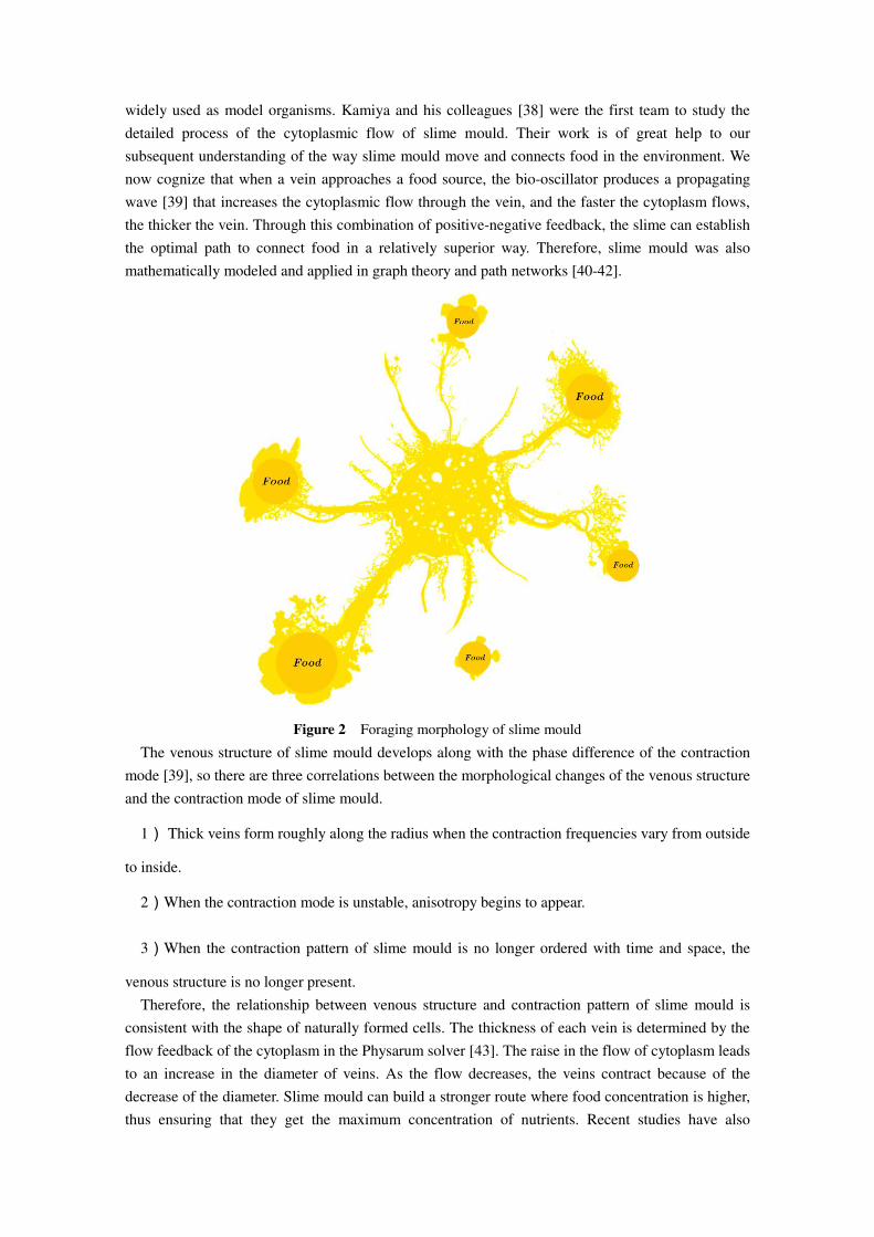
to flow inside [36], as shown in Figure 2. Because of their unique pattern and characteristic, they

can use multiple food sources at the same time to form a venous network connecting them. If there is

enough food in the environment, slime mould can even grow to more than 900 square centimeters

[36].

Owing to the feature of slime mould can be easily cultured on agar and oatmeal [37], they were

widely used as model organisms. Kamiya and his colleagues [38] were the first team to study the

detailed process of the cytoplasmic flow of slime mould. Their work is of great help to our

subsequent understanding of the way slime mould move and connects food in the environment. We

now cognize that when a vein approaches a food source, the bio-oscillator produces a propagating

wave [39] that increases the cytoplasmic flow through the vein, and the faster the cytoplasm flows,

the thicker the vein. Through this combination of positive-negative feedback, the slime can establish

the optimal path to connect food in a relatively superior way. Therefore, slime mould was also

mathematically modeled and applied in graph theory and path networks [40-42].

Figure 2 Foraging morphology of slime mould

The venous structure of slime mould develops along with the phase difference of the contraction

mode [39], so there are three correlations between the morphological changes of the venous structure

and the contraction mode of slime mould.

1） Thick veins form roughly along the radius when the contraction frequencies vary from outside

to inside.

2）When the contraction mode is unstable, anisotropy begins to appear.

3）When the contraction pattern of slime mould is no longer ordered with time and space, the

venous structure is no longer present.

Therefore, the relationship between venous structure and contraction pattern of slime mould is

consistent with the shape of naturally formed cells. The thickness of each vein is determined by the

flow feedback of the cytoplasm in the Physarum solver [43]. The raise in the flow of cytoplasm leads

to an increase in the diameter of veins. As the flow decreases, the veins contract because of the

decrease of the diameter. Slime mould can build a stronger route where food concentration is higher,

thus ensuring that they get the maximum concentration of nutrients. Recent studies have also

revealed that slime mould have the competence of making foraging arrangements based on

optimization theory [44]. When the quality of various food sources is different, slime mould can

choose the food source with the highest concentration. However, slime mould also needs to weigh

speed and risk in foraging. For instance, slime mould needs to make faster decisions in order to

avoid environmental damage to them. Experiments have shown that the quicker the decision-making

speed is, the possibilities of slime mould to find the prime food source is smaller [45]. Therefore,

when deciding the source of food, slime mould obviously needs to weigh the speed and accuracy.

Slime mould need to decide when to leave this area and search in another area when foraging.

When lacking complete information, the best way for a slime mould to estimate when to leave the

current position is to adopt heuristic or empirical rules based on the insufficient information

currently available. Experience has shown that when slime mould encounter high-quality food, the

probability of leaving the area is reduced [46]. However, due to its unique biological characteristics,

slime mould can utilize a variety of food sources at the same time. Therefore, even if the slime

mould has found a better source of food, it can still divide a component of the biomass to exploit

both resources simultaneously when higher quality food is found [43].

Slime mould can also dynamically adjust their search patterns according to the quality of foodstuff

provenience. When the quality of food sources is high, the slime mould will use the region-limited

search method [47], thus focusing the search on the food sources that have been found. If the

denseness of the food provenience initially found is low, the slime mould will leave the food source

to explore other alternative food sources in the region [48]. This adaptive search strategy can be

more reflected when different quality food blocks are dispersed in a region. Some of the mechanisms

and characteristics of the slime mould mentioned above will be mathematically modeled in the

subsequent sections.

2.3 Mathematical model

In this part, the mathematical model and method proposed will be described in details.

2.3.1 Approach food

Slime mould can approach food according to the odor in the air. To express its approaching behavior

in mathematical formulas, the following formulas are proposed to imitate the contraction mode:

𝑋(𝑡 + 1)⃗⃗ ⃗⃗ ⃗⃗ ⃗⃗ ⃗⃗ ⃗⃗ ⃗⃗ ⃗⃗ ⃗ = {𝑋𝑏(𝑡)⃗⃗⃗⃗ ⃗⃗ ⃗⃗ ⃗⃗ ⃗ + 𝑣𝑏⃗⃗⃗⃗ ∙ .�⃗⃗⃗� ∙ 𝑋𝐴(𝑡)⃗⃗ ⃗⃗ ⃗⃗ ⃗⃗ ⃗⃗ − 𝑋𝐵(𝑡)⃗⃗ ⃗⃗ ⃗⃗ ⃗⃗ ⃗⃗ ⃗/ , 𝑟 < 𝑝𝑣𝑐⃗⃗⃗⃗ ∙ 𝑋(𝑡)⃗⃗ ⃗⃗ ⃗⃗ ⃗⃗ , 𝑟 ≥ 𝑝 (2.1)

where 𝑣𝑏⃗⃗ ⃗⃗ ⃗ is a parameter with a range of ,−𝑎, 𝑎- , 𝑣𝑐⃗⃗⃗⃗ decreases linearly from one to zero. 𝑡 represents the current iteration, 𝑋𝑏⃗⃗ ⃗⃗ ⃗ represents the individual location with the highest odor

concentration currently found, 𝑋 represents the location of slime mould, 𝑋𝐴⃗⃗ ⃗⃗ and 𝑋𝐵⃗⃗ ⃗⃗ represent two

individuals randomly selected from slime mould, �⃗⃗⃗� represents the weight of slime mould.

The formula of 𝑝 is as follows: 𝑝 = tanh|𝑆(𝑖) − 𝐷𝐹| (2.2)

where 𝑖 ∈ 1,2,… , 𝑛, 𝑆(𝑖) represents the fitness of 𝑋 , 𝐷𝐹 represents the best fitness obtained in all

iterations.

The formula of 𝑣𝑏⃗⃗⃗⃗ is as follows: 𝑣𝑏⃗⃗⃗⃗ = ,−𝑎, 𝑎- (2.3)

𝑎 = arctanh (−( 𝑡max _𝑡) + 1) (2.4)

The formula of �⃗⃗⃗� is listed as follows:

𝑊(𝑆𝑚𝑒𝑙𝑙𝐼𝑛𝑑𝑒𝑥(𝑖))⃗⃗ ⃗⃗ ⃗⃗ ⃗⃗ ⃗⃗ ⃗⃗ ⃗⃗ ⃗⃗ ⃗⃗ ⃗⃗ ⃗⃗ ⃗⃗ ⃗⃗ ⃗⃗ ⃗⃗ ⃗⃗ ⃗⃗ ⃗⃗ ⃗⃗ ⃗⃗ = { 1 + 𝑟 ∙ 𝑙𝑜𝑔 (𝑏𝐹 − 𝑆(𝑖)𝑏𝐹 − 𝑤𝐹 + 1) , 𝑐𝑜𝑛𝑑𝑖𝑡𝑖𝑜𝑛 1 − 𝑟 ∙ 𝑙𝑜𝑔 (𝑏𝐹 − 𝑆(𝑖)𝑏𝐹 − 𝑤𝐹 + 1) , 𝑜𝑡𝑕𝑒𝑟𝑠 (2.5)

𝑆𝑚𝑒𝑙𝑙𝐼𝑛𝑑𝑒𝑥 = 𝑠𝑜𝑟𝑡(𝑆) (2.6)

where 𝑐𝑜𝑛𝑑𝑖𝑡𝑖𝑜𝑛 indicates that 𝑆(𝑖) ranks first half of the population，𝑟 denotes the random value

in the interval of ,0,1-，𝑏𝐹 denotes the optimal fitness obtained in the current iterative process, 𝑤𝐹 denotes the worst fitness value obtained in the iterative process currently, 𝑆𝑚𝑒𝑙𝑙𝐼𝑛𝑑𝑒𝑥 denotes

the sequence of fitness values sorted(ascends in the minimum value problem).

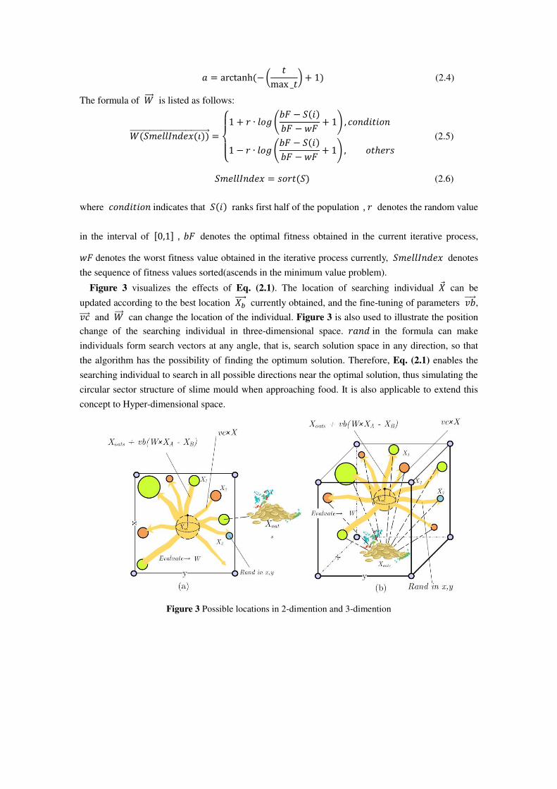
Figure 3 visualizes the effects of Eq. (2.1). The location of searching individual 𝑋 can be

updated according to the best location 𝑋𝑏⃗⃗ ⃗⃗ currently obtained, and the fine-tuning of parameters 𝑣𝑏⃗⃗⃗⃗ , 𝑣𝑐⃗⃗⃗⃗ and �⃗⃗⃗� can change the location of the individual. Figure 3 is also used to illustrate the position

change of the searching individual in three-dimensional space. 𝑟𝑎𝑛𝑑 in the formula can make

individuals form search vectors at any angle, that is, search solution space in any direction, so that

the algorithm has the possibility of finding the optimum solution. Therefore, Eq. (2.1) enables the

searching individual to search in all possible directions near the optimal solution, thus simulating the

circular sector structure of slime mould when approaching food. It is also applicable to extend this

concept to Hyper-dimensional space.

Figure 3 Possible locations in 2-dimention and 3-dimention

Figure 4 Assessment of fitness

2.3.2 Wrap food

This part simulates the contraction mode of venous tissue structure of slime mould mathematically

when searching. The higher the concentration of food contacted by the vein, the stronger the wave

generated by the bio-oscillator, the faster the cytoplasm flows, and the thicker the vein. Eq. (2.5)

mathematically simulated the positive and negative feedback between the vein width of the slime

mould and the food concentration that was explored. The component 𝑟 in Eq. (2.5) simulates the

uncertainty of venous contraction mode. 𝑙𝑜𝑔 is used to alleviate the change rate of numerical value

so that the value of contraction frequency does not change too much. 𝑐𝑜𝑛𝑑𝑖𝑡𝑖𝑜𝑛 simulates the slime

mould to adjust their search patterns according to the quality of food. When the food concentration is

content, the bigger the weight near the region is; when the food concentration is low, the weight of

the region will be reduced, thus turning to explore other regions. Figure 4 shows the process of

evaluating fitness values for slime mould.

Based on the above principle, the mathematical formula for updating the location of slime mould

is as follows:

𝑋∗⃗⃗ ⃗⃗ = { 𝑟𝑎𝑛𝑑 ∙ (𝑈𝐵 − 𝐿𝐵) + 𝐿𝐵, 𝑟𝑎𝑛𝑑 < 𝑧 𝑋𝑏(𝑡)⃗⃗⃗⃗ ⃗⃗ ⃗⃗ ⃗⃗ ⃗ + 𝑣𝑏⃗⃗⃗⃗ ∙ .𝑊 ∙ 𝑋𝐴(𝑡)⃗⃗ ⃗⃗ ⃗⃗ ⃗⃗ ⃗⃗ − 𝑋𝐵(𝑡)⃗⃗ ⃗⃗ ⃗⃗ ⃗⃗ ⃗⃗ ⃗/ , 𝑟 < 𝑝 𝑣𝑐⃗⃗⃗⃗ ∙ 𝑋(𝑡)⃗⃗ ⃗⃗ ⃗⃗ ⃗⃗ , 𝑟 ≥ 𝑝 (2.7)

where 𝐿𝐵 and 𝑈𝐵 denote the lower and upper boundaries of search range, 𝑟𝑎𝑛𝑑 and 𝑟 denote the

random value in [0,1]. The value of 𝑧 will be discussed in the parameter setting experiment.

2.3.3 Grabble food

Slime mould mainly depends on the propagation wave produced by the biological oscillator to

change the cytoplasmic flow in veins, so that they tend to be in a better position of food

concentration. On the purpose of simulating the variations of venous width of slime mould, we used �⃗⃗⃗� , 𝑣𝑏⃗⃗⃗⃗ and 𝑣𝑐⃗⃗⃗⃗ to realize the variations. �⃗⃗⃗� mathematically simulates the oscillation frequency of slime mould near one at different food

concentration, so that slime mould can approach food more quickly when they find high-quality food,

while approach food more slowly when the food concentration is lower in individual position, thus

improving the efficiency of slime mould in choosing the optimal food source.

The value of 𝑣𝑏⃗⃗⃗⃗ oscillates randomly between ,−𝑎, 𝑎- and gradually approaches zero as the

increasement of iterations. The value of 𝑣𝑐⃗⃗⃗⃗ oscillates between [-1,1] and tends to zero eventually.

The trend of the two values is shown as Figure 5. Synergistic interaction between 𝑣𝑏⃗⃗⃗⃗ and 𝑣𝑐⃗⃗⃗⃗ mimics the selective behavior of slime mould. In order to find a better source of food, even if slime

mould has found a better source of food, it will still separate some organic matter for exploring other

areas in an attempt to find a higher quality source of food, rather than investing all of it in one

source.

Figure 5 Trends of 𝑣𝑏⃗⃗⃗⃗ and 𝑣𝑐⃗⃗⃗⃗ Moreover, the oscillation process of 𝑣𝑏⃗⃗⃗⃗ simulates the state of slime mould deciding whether to

approach the food source or find other food sources. Meanwhile, the process of probing food is not

smooth. During this period, there may be various obstacles, such as light and dry environment,

which restrict the spread of slime mould. However, it also improves the possibility of slime mould to

find higher quality food and evades the trapping of local optimum.

The pseudo code of the SMA is shown in Algorithm 1. The intuitive and detailed process of SMA

is shown in Figure 6.

There are still many mechanisms that can be added to the algorithm, or more comprehensive

simulation of the life cycle of slime mould. However, to enhance the extensibility of the algorithm,

we simplify the process and operators of the algorithm, leaving only the simplest algorithm as

possible.

Algorithm 1 Pseudo-code of SMA

Initialize the parameters popsize, 𝑀𝑎𝑥_𝑖𝑡𝑒𝑟𝑎𝑖𝑡𝑖𝑜𝑛;

Initialize the positions of slime mould 𝑋𝑖(𝑖 = 1,2,… , 𝑛); While (𝑡 ≤ 𝑀𝑎𝑥_𝑖𝑡𝑒𝑟𝑎𝑖𝑡𝑖𝑜𝑛)

Calculate the fitness of all slime mould; 𝑢𝑝𝑑𝑎𝑡𝑒 𝑏𝑒𝑠𝑡𝐹𝑖𝑡𝑛𝑒𝑠𝑠, 𝑋𝑏

Calculate the W by Eq. (2.5);

For 𝑒𝑎𝑐𝑕 𝑠𝑒𝑎𝑟𝑐𝑕 𝑝𝑜𝑟𝑡𝑖𝑜𝑛

𝑢𝑝𝑑𝑎𝑡𝑒 𝑝, 𝑣𝑏, 𝑣𝑐; 𝑢𝑝𝑑𝑎𝑡𝑒 𝑝𝑜𝑠𝑖𝑡𝑖𝑜𝑛𝑠 𝑏𝑦 𝐄𝐪. (2.7); End 𝐅𝐨𝐫 𝑡 = 𝑡 + 1;

End While

Return 𝑏𝑒𝑠𝑡𝐹𝑖𝑡𝑛𝑒𝑠𝑠, 𝑋𝑏;

2.3.4 Computational complexity analysis

SAM mainly consists of the subsequent components: initialization, fitness evaluation, and sorting,

weight update, and location update. Among them, N denotes the number of cells of slime mould, D

denotes the dimension of functions, and T denotes the maximum number of iterations. The

computation complexity of initialization is 𝛰(𝑁), the computation complexity of fitness evaluation

and sorting is 𝛰(𝑁 +𝑁 𝑙𝑜𝑔𝑁), the computational complexity of weight update is 𝛰(𝑁 × 𝐷), the

complexity of location update is 𝛰(𝑁 × 𝐷). Therefore, the total complexity of SMA is 𝛰(𝑁 ∗ (1 +𝑇 ∗ 𝑁 ∗ (1 + 𝑙𝑜𝑔𝑁 + 2 ∗ 𝐷))).

Figure 6 Flowchart of SMA

3 Experimental results and analyses

In this sector, we compared the SMA with some competitive MAs in an all-inclusive set of 33

benchmarks. The experimentations were ran on the operating system of Windows Server 2012 R2

Datacenter with 128 GB RAM and CPU of Intel (R) Xeon (R) E5-2650 v4 (2.20 GHz). The

algorithms for comparison were coded by MATLAB R2018b.

3.1 Qualitative analysis

The qualitative analysis results of SMA in handling unimodal functions and multimodal functions

are presented in Figure 7 to intuitively analyze the position and fitness changes of slime mould

during foraging. The figure is comprised of four concernment indicators: search history, the

trajectory of the slime mould in the 1st dimension, the average fitness of slime mould, and

convergence curve. Search history represents the location and distribution of slime mould in the

iteration process. The trajectory of slime mould reveals the behavior of the position change of slime

mould in the first part of the first dimension. Average fitness indicates the variation trend of the

average fitness of the slime mould colony changes with the iteration process. Convergence curve

shows the optimal fitness value in the slime mould during the iteration process.

From the search history subplot, the slime mould in different benchmark functions put up a similar

cross-type search trajectory clustered near the optimal value, thus accurately searching in reliable

search areas and reflecting fast convergence. Meanwhile, the distribution of slime mould is mainly

concentrated in multiple regions with local optimum, which shows the tradeoff of slime mould

between multiple local optimums.

The trajectory of the first slime mould in the first dimension can be used as a representative of

other parts of slime mould, revealing the primary exploratory behavior of slime mould. The fast

oscillation in the prophase and the slight oscillation in the anaphase can ensure the fast convergence

of slime mould and the accurate search near the optimal solution [49]. As can be perceived from the

figure, the position curve of slime mould has very large amplitude in the early iteration process, even

up to 50% of the exploration space. In the later iteration period, if the function is smooth, the

amplitude of the position of slime mould begins to decrease; if the amplitude of the function changes

significantly, the position amplitude also changes greatly. This reflects the high adaptability and

robustness of slime mould in different functions.

By observing the average fitness curve, the variation tendency of the fitness of slime mould during

the iterative procedure can be visually observed. Although the average fitness curve of slime mould

is oscillating, the average fitness value tends to decrease, and the oscillation frequency decreases

inversely proportional to iterations, thus ensuring the rapid convergence of slime mould in the

prophase and the precise search in the anaphase.

Convergence curve reveals the average fitness of the optimal fitness value searched by slime

mould varies with iterations. By observing the downtrend of the curve, we can observe the

convergence rate of slime mould and the time when it switches between the exploration and

exploration gradation.

Figure 7 Qualitative analysis

3.2 Benchmark function validation

In this section, SMA was assessed on a comprehensive set of functions from 23 benchmarks and

CEC 2014. These functions cover unimodal, multimodal, hybrid, and composite functions, as shown

in Tables 1-3. Some composite functions of CEC 2014 are shown in Figure 8. Dim denotes the

dimension of function; Range denotes the definition domain of the function, and 𝑓𝑚𝑖𝑛 denotes the

optimal value of the function. The MAs used for comparison include well-regarded and recent ones:

WOA [50], GWO [21], MFO [23], BA [20], SCA [7], FA[51], PSO[18], SSA [52], MVO [3], ALO

[53], PBIL [54], DE [55] and advanced MAs: AGA[56], BLPSO [57], CLPSO [58], CBA [59],

RCBA [60], CDLOBA [61], m_SCA [62], IWOA [63], LWOA [64], and CSSA [65]. The parameter

setup of traditional MAs is detailed in Table 4. The parameter selection was based on the parameters

used by the original author in the article or the parameters widely used by various researchers.

Figure 8 Illustration of CEC 2014 composite functions

Table 1

Unimodal and multimodal test functions of 23 standard benchmarks

Functions Dim Range 𝑓𝑚𝑖𝑛 𝑓 (𝑥) = ∑ 𝑥𝑖 𝑛𝑖 n [-100,100] 0 𝑓 (𝑥) = ∑ 𝑥𝑖𝑛𝑖 +∏ 𝑥𝑖𝑛𝑖 n [-10,10] 0 𝑓 (𝑥) = ∑ (∑ 𝑥 𝑖 ) 𝑛𝑖 n [-100,100] 0 𝑓 (𝑥) = 𝑚𝑎𝑥𝑖* 𝑥𝑖 ,1 ≤ 𝑖 ≤ 𝑛+ n [-100,100] 0 𝑓 (𝑥) = ∑ ,100(𝑥𝑖 − 𝑥𝑖 ) + (𝑥𝑖 − 1) -𝑛 𝑖 n [-30,30] 0 𝑓 (𝑥) = ∑ (,𝑥𝑖 + 0.5-) 𝑛𝑖 n [-100,100] 0 𝑓 (𝑥) = ∑ 𝑖𝑥𝑖 + 𝑟𝑎𝑛𝑑𝑜𝑚,0,1-𝑛𝑖 n [-128,128] 0 𝑓 (𝑥) = ∑ −𝑥𝑖 n(√ 𝑥𝑖 )𝑛𝑖 n [-500,500] -418.9829*n 𝑓 (𝑥) = ∑ ,𝑥𝑖 − 10 co (2 𝑥𝑖) + 10-𝑛𝑖 n [-5.12,5.12] 0 𝑓 (𝑥) = −20 xp (−0.2( 𝑛∑ 𝑥𝑖 𝑛𝑖 ) 0.5) − xp . 𝑛∑ co (2 𝑥𝑖)𝑛𝑖 / + 20 + 𝑒 n [-32,32] 0 𝑓 (𝑥) = ∑ 𝑥𝑖 𝑛𝑖 −∏ co . √𝑖/𝑛𝑖 + 1 n [-600,600] 0 𝑓 (𝑥) = 𝑛 *10 n( 𝑦 ) + ∑ (𝑦𝑖 − 1) ,1 + 10 n ( 𝑦𝑖 )-𝑛 𝑖 + (𝑦𝑛 − 1) + +∑ 𝑢(𝑥𝑖 , 10,100,4)𝑛𝑖 , 𝑦𝑖 = 1 +

𝑢(𝑥𝑖 , 𝑎, ,𝑚) = { (𝑥𝑖 − 𝑎)𝑚 𝑥𝑖 𝑎0 − 𝑎 < 𝑥𝑖 < 𝑎 (−𝑥𝑖 − 𝑎)𝑚 𝑥𝑖 < 𝑎

n [-50,50] 0

𝑓 (𝑥) = 0.1* n (3 𝑥 ) +∑ (𝑥𝑖 − 1) ,1 + n (3 𝑥𝑖 + 1)-𝑛𝑖 + (𝑥𝑛 − 1) ,1 + n (2 𝑥𝑛)-+ + ∑ 𝑢(𝑥𝑖 , 5,100,4)𝑛𝑖 n [-50,50] 0

Table 2

Unimodal and simple multimodal functions of CEC2014

Functions Dim Range 𝑓𝑚𝑖𝑛 𝑓 (𝑥) = otat h on t on pt c nct on n [-100,100] 100 𝑓 (𝑥) = otat nt ar nct on n [-100,100] 200 𝑓 (𝑥) = h t an otat ( ) c nct on n [-100,100] 500 𝑓 (𝑥) = r tra nct on n [-100,100] 600 𝑓 (𝑥) = app at nct on n [-100,100] 1300 𝑓 (𝑥) = at nct on n [-100,100] 1400 𝑓 (𝑥) = xpan r an p o n roc nct on n [-100,100] 1500

𝑓 (𝑥) = xpan ca r 6 nct on n [-100,100] 1600

Table 3

Hybrid and Composition functions of CEC 2014

Functions Dim Range 𝑓𝑚𝑖𝑛 𝑓 (𝑥) = r nct on 1 n [-100,100] 1700 𝑓 (𝑥) = r nct on 2 n [-100,100] 1800 𝑓 (𝑥) = r nct on 3 n [-100,100] 1900 𝑓 (𝑥) = r nct on 4 n [-100,100] 2000 𝑓 (𝑥) = r nct on 5 n [-100,100] 2100 𝑓 (𝑥) = r nct on 6 n [-100,100] 2200 𝑓 (𝑥) = ompo t nct on 1 n [-100,100] 2300 𝑓 (𝑥) = ompo t nct on 2 n [-100,100] 2400 𝑓 (𝑥) = ompo t nct on 3 n [-100,100] 2500 𝑓 (𝑥) = ompo t nct on 4 n [-100,100] 2600 𝑓 (𝑥) = ompo t nct on 5 n [-100,100] 2700 𝑓 (𝑥) = ompo t nct on 6 n [-100,100] 2800

Table 4

Parameter settings of counterparts

Algorithm Parameter settings

WOA 𝑎 = ,2,0-; 𝑎 = ,−2,−1-; 𝑏 = 1

GWO 𝑎 = ,2,0-

MFO 𝑏 = 1; 𝑡 = ,−1,1-; 𝑎 ∈ ,−1,−2-

BA 𝐴 = 0.5; 𝑟 = 0.5

SCA 𝐴 = 2

FA 𝛼 = 0.5; 𝛽 = 0.2; 𝛾 = 1

PSO 𝑐 = 2; 𝑐 = 2; 𝑣𝑀𝑎𝑥 = 6

SSA 𝑐 ∈ ,0 1-; 𝑐 ∈ ,0 1-;

MVO 𝑒𝑥𝑖𝑠𝑡𝑒𝑛𝑐𝑒 𝑝𝑟𝑜𝑏𝑎𝑏𝑖𝑙𝑖𝑡𝑦 ∈ ,0.2 1-; 𝑡𝑟𝑎𝑣𝑒𝑙𝑙𝑖𝑛𝑔 𝑑𝑖𝑠𝑡𝑎𝑛𝑐𝑒 𝑟𝑎𝑡𝑒 ∈ ,0.6 1-

ALO = 500

PBIL 𝑙𝑒𝑎𝑟𝑛𝑖𝑛𝑔 𝑟𝑎𝑡𝑒 = 0.05; 𝑒𝑙𝑖𝑡𝑖𝑠𝑚 𝑝𝑎𝑟𝑎𝑚𝑒𝑡𝑒𝑟 = 1; 𝑝𝑟𝑜𝑏𝑎𝑏𝑖𝑙𝑖𝑡𝑦 𝑣𝑒𝑐𝑡𝑜𝑟 𝑚𝑢𝑡𝑎𝑡𝑖𝑜𝑛 𝑟𝑎𝑡𝑒 = 0

DE 𝑠𝑐𝑎𝑙𝑖𝑛𝑔 𝑓𝑎𝑐𝑡𝑜𝑟 = 0.5; 𝑐𝑟𝑜𝑠𝑠𝑜𝑣𝑒𝑟 𝑝𝑟𝑜𝑏𝑎𝑏𝑖𝑙𝑖𝑡𝑦 = 0.5

All algorithms were performed under the same conditions to achieve fairness in comparative

experiments. Among them, the population was set to 30, the dimension and the iteration time was set

to 30 and 1000 respectively. To reduce the impacts of random factors in the algorithm on the results,

all the compared algorithms were run individually 30 times in each function and averaged as the

final running result. On the purpose of measuring experiment results, Standard deviation (STD),

Average results (AVG) and Median (MED) were employed to evaluate the results. Note that best

results will be bolded (take one in the case of juxtaposition).

3.2.1 Exploitation competence analysis

The data in Table 5 demonstrates that SMA ranked first or tied first on average when solving F1-5,

F7, and F14. The convergence curves of F2 and F5 in Figure 9 can be visually observed that SMA

has the fastest convergence trend among all the comparative functions. The data in Table 6

demonstrates that SMA can still exhibit significant advantages even when compared to a modified

Ma, such as ranking first among other unimodal functions other than F5 and F14. These functions

are unimodal functions in the benchmarks, reflecting SMA's efficient exploration capability.

Moreover, in order to more fairly evaluate the local search efficiency of the algorithm, an evaluation

version of the experiment has been added. The data in Table 7 demonstrate the experimental results

obtained by 300,000 evaluations of the SMA with 10 other participants on the unimodal functions. In

the experimental results, the values obtained by SMA were still better than those of other algorithms

on F1-5 and F7. At the same time, the median values of the solutions were also consistent with the

ranking of the optimal values, indicating the stability of the SMA.

Table 5

Comparison results on unimodal functions with traditional algorithms during 1000 iterations

F1 F2 F3

Algorithm AVG STD MED AVG STD MED AVG STD MED

SMA 0.000000 0.000000 1.08E-64 5.330E-207 0.000000 5.93E-58 0.00000 0.00000 8.22E-02

SCA 0.015244 0.029989 9.36E+01 1.150E-05 2.743E-05 8.06E-03 3261.99676 2935.03792 2.75E+04

SSA 1.231E-08 3.536E-09 1.83E+02 0.848146 0.941518 8.90E+00 236.62194 155.54710 2.94E+03

GWO 4.223E-59 1.081E-58 4.39E-46 1.128E-34 9.149E-35 7.07E-28 4.027E-15 1.418E-14 1.50E-09

MFO 2000.0006 4068.3807 2.04E+03 33.666839 20.253973 3.42E+01 24900.5554 14138.0477 2.91E+04

WOA 4.322E-153 2.276E-152 2.34E-54 5.032E-104 1.591E-103 3.42E-34 20802.2782 10554.3925 5.30E+04

GOA 7.670196 6.676643 1.27E+03 9.540510 14.128406 3.09E+01 1794.1195 1103.3922 7.64E+03

DA 1158.4940 600.8920 1.19E+03 14.313148 5.649106 1.45E+01 9612.3629 6188.5858 9.64E+03

ALO 1.050E-05 7.825E-06 7.10E+00 28.698940 42.100743 3.02E+01 1275.7431 596.2918 1.73E+03

MVO 0.318998 0.112060 9.40E+02 0.388930 0.137834 1.39E+01 48.11246 21.77526 4.61E+03

PBIL 46908.0000 4218.6045 4.84E+04 95.200000 5.892134 9.80E+01 54824.1 6552.855378 6.02E+04

PSO 128.803704 15.368375 1.42E+02 86.075426 65.298810 1.12E+02 406.96260 71.30926 6.06E+02

DE 3.030E-12 3.454E-12 4.01E-04 3.723E-08 1.196E-08 2.24E-03 24230.5748 4174.3788 3.00E+04

F4 F5 F6


SMA 2.301E-197 0.000000 1.31E-25 0.42779 0.63700 9.89E+00 0.000879 0.000415 5.97E-01

SCA 20.532489 11.046644 7.53E+01 532.7126 1907.4456 1.58E+06 4.550121 0.357049 3.37E+01

SSA 8.254602 3.287966 1.62E+01 135.5698 174.1213 7.77E+03 0.000000 0.000000 2.04E+02

GWO 1.776E-14 2.228E-14 9.01E-12 27.10029 0.86432 2.73E+01 0.726058 0.278337 9.75E-01

MFO 64.420279 8.689356 6.47E+01 5348258 20289785 5.35E+06 1656.708 5277.651 1.68E+03

WOA 45.706343 26.935040 4.61E+01 27.26543 0.57447 2.73E+01 0.100557 0.110525 1.01E-01

GOA 12.596514 4.317304 2.35E+01 1631.1583 2241.1368 2.58E+05 4.884661 4.512327 1.36E+03

DA 23.631736 8.191777 2.37E+01 127371 96386 1.31E+05 1330.292 632.470 1.34E+03

ALO 12.133214 3.585375 1.32E+01 298.8031 431.1446 5.00E+02 0.000012 0.000011 7.49E+00

MVO 1.076968 0.310884 1.40E+01 407.9465 615.3290 8.63E+04 0.323756 0.097394 9.34E+02

PBIL 79.666667 4.088110 8.00E+01 143346156 31547349 1.51E+08 45881.833 4850.932 4.77E+04

PSO 4.498158 0.329339 4.79E+00 154736 36039 1.85E+05 132.779 15.189 1.45E+02

DE 1.965929 0.430531 1.32E+01 46.12942 27.29727 1.40E+02 3.096E-12 1.461E-12 4.11E-04

F7 F14 F15


SMA 8.839E-05 7.118E-05 4.08E-04 9549563 6529870 2.97E+07 22233.8245 14144.9575 5.47E+07

SCA 0.024382 0.020732 6.04E-01 425718766 116756947 7.06E+08 2.689E+10 5.427E+09 3.97E+10

SSA 0.095541 0.050530 1.59E-01 20297116 8153518 6.91E+07 11222.8121 11173.7583 3.37E+08

GWO 0.000869 0.000435 1.46E-03 88751868 66700399 1.29E+08 2.254E+09 1.759E+09 3.98E+09

MFO 4.620163 13.076256 4.77E+00 87010749 137363574 1.00E+08 1.341E+10 7.685E+09 1.35E+10

WOA 0.000986 0.001147 2.66E-03 160431438 69271930 1.62E+08 2.154E+09 1.086E+09 2.17E+09

GOA 0.024028 0.011253 2.96E-02 33807500 14819986 1.28E+08 17667580 11032455 2.34E+09

DA 0.326978 0.138556 3.31E-01 305164519 121919102 3.05E+08 6.363E+09 2.751E+09 6.37E+09

ALO 0.103373 0.034257 1.06E-01 12505761 5184932 1.69E+07 12378 9058 1.25E+07

MVO 0.020859 0.009584 1.42E-01 14860094 6244884 5.89E+07 566570 210025 1.45E+09

PBIL 282.1349 43.2693 2.93E+02 574020990 128317251 7.02E+08 4.961E+10 5.107E+09 5.32E+10

PSO 111.0068 21.5378 1.11E+02 17174833 5483990 2.16E+07 191733286 23903821 2.09E+08

DE 0.026937 0.006322 5.44E-02 100597441 31636302 1.78E+08 1601.8022 3314.1727 1.97E+05

Table 6

Comparison results on the unimodal functions with advanced algorithms

F1 F2 F3


SMA 0.000000 0.000000 4.72E-37 4.20E-187 0.000000 1.24E-66 0.000000 0.000000 1.19E-02

BLPSO 2208.3313 397.7883 5.00E+03 17.665054 1.905407 3.35E+01 13540.48 1672.45 1.82E+04

CLPSO 596.7364 150.3595 5.15E+03 11.846531 1.669288 4.09E+01 16836.42 3085.75 2.71E+04

CBA 0.113583 0.454545 4.38E-01 305804 1652847 5.73E+05 73.709725 31.029467 2.54E+02

RCBA 0.201488 0.052889 5.31E-01 10.958358 28.471304 2.77E+01 95.544912 43.376020 7.44E+02

CDLOBA 0.005957 0.002133 1.88E-02 3781.932 15086.168 1.24E+04 1.791342 6.166318 3.50E+02

m_SCA 2.521E-46 1.378E-45 8.14E-04 3.478E-33 1.420E-32 2.01E-06 8.991E-16 3.188E-15 5.82E+03

IWOA 8.130E-146 4.370E-145 1.00E-53 2.385E-102 6.585E-102 1.44E-33 15410.3 7420.1 3.62E+04

LWOA 6.743E-07 7.589E-07 1.55E-01 2.801E-07 3.833E-07 6.54E-02 43293.10 13505.91 9.25E+04

CSSA 0.017344 0.027805 1.74E-02 0.061732 0.027609 6.21E-02 2.926441 3.133898 2.95E+00

F4 F5 F6


SMA 8.84E-183 0.00000 1.80E-36 1.27571 4.90297 1.22E+01 0.000880 0.000407 9.26E-01

BLPSO 27.66310 2.40967 3.54E+01 520889 178483 2.75E+06 2207.564 410.182 5.20E+03

CLPSO 42.44490 4.41014 5.61E+01 113820 39571 2.95E+06 563.251 138.054 5.26E+03

CBA 17.03820 7.72324 2.20E+01 197.6163 360.2440 2.58E+02 0.001823 0.007886 1.16E-01

RCBA 9.00594 3.41186 1.49E+01 148.2466 122.4613 2.29E+02 0.187352 0.054118 4.62E-01

CDLOBA 46.10460 7.48538 4.81E+01 138.1210 178.6248 2.29E+02 0.005940 0.001899 1.79E-02

m_SCA 2.248E-13 1.223E-12 1.53E+01 27.62609 0.84321 3.34E+01 2.540097 0.499546 4.06E+00

IWOA 13.12456 16.19609 2.26E+01 26.57003 0.66075 2.70E+01 0.036361 0.069578 6.17E-02

LWOA 11.12439 14.63066 2.69E+01 25.63874 6.59153 2.90E+01 0.009637 0.002992 4.25E-01

CSSA 0.03301 0.01983 3.45E-02 0.17508 0.16603 1.76E-01 0.030982 0.062573 3.11E-02

F7 F14 F15


SMA 8.21E-05 7.16E-05 3.24E-04 9689581 7904687 3.20E+07 15808.97 10533.48 5.40E+07

BLPSO 0.59346 0.17290 1.50E+00 1.72E+08 3.74E+07 2.98E+08 3.718E+09 5.932E+08 8.78E+09

CLPSO 0.26201 0.05157 1.74E+00 1.77E+08 6.19E+07 4.28E+08 1.985E+09 4.391E+08 1.47E+10

CBA 0.47023 0.31242 7.47E-01 1.15E+07 5802441 1.80E+07 513564.79 1056309.50 2.80E+06

RCBA 0.61360 0.25709 1.02E+00 5943596 2275351 1.06E+07 372942.94 107512.69 8.44E+05

CDLOBA 26.93780 39.54585 6.71E+01 4469831 2849244 1.07E+07 18462.13 9920.05 3.57E+04

m_SCA 0.00071 0.00053 2.02E-02 1.15E+08 6.69E+07 3.52E+08 1.048E+10 4.703E+09 2.38E+10

IWOA 0.00185 0.00236 3.92E-03 9.34E+07 4.72E+07 1.19E+08 1.047E+09 8.576E+08 1.43E+09

LWOA 0.00650 0.00439 3.44E-02 8.81E+07 3.31E+07 4.11E+08 3.334E+08 1.326E+08 2.21E+10

CSSA 0.00019 0.00016 6.78E-04 1.68E+09 2.36E+08 1.68E+09 8.837E+10 6.958E+09 8.84E+10

Table 7

Comparison results on unimodal functions during 3E5 evaluations

F1 F2 F3


SMA 0.00000 0.00000 2.150E-268 0.00000 0.00000 1.999E-141 0.00000 0.00000 7.427E-244

SCA 5.33E-52 2.92E-51 1.325E-19 3.28E-60 9.54E-60 1.256E-28 2.65E+00 1.03E+01 2.763E+03

SSA 3.97E-09 7.20E-10 6.629E+01 2.20E-01 5.24E-01 4.818E+00 6.21E-08 1.97E-08 5.697E+02

GWO 0.00000 0.00000 0.000E+00 0.00000 0.00000 1.002E-286 8.62E-174 0.00000 1.908E-125

MFO 1.67E+03 3.79E+03 1.667E+03 3.53E+01 2.45E+01 3.533E+01 1.58E+04 1.08E+04 1.579E+04

WOA 0.00000 0.00000 0.000E+00 0.00000 0.00000 0.000E+00 2.15E+01 5.44E+01 1.755E+03

GOA 1.37E-03 7.51E-04 7.244E+02 4.93E-01 5.10E-01 1.954E+01 1.15E+02 3.94E+02 2.836E+03

MVO 3.11E-03 7.04E-04 5.957E+02 3.84E-02 1.30E-02 1.113E+01 3.70E-01 1.10E-01 1.613E+03

PSO 1.01E+02 1.43E+01 1.113E+02 4.69E+01 3.54E+00 5.156E+01 1.85E+02 2.76E+01 2.205E+02

DE 1.46E-159 3.86E-159 4.314E-76 2.02E-94 2.33E-94 1.359E-45 1.39E+03 7.73E+02 6.275E+03

AGA 2.38E-02 2.48E-02 5.567E-02 1.18E-02 3.99E-03 1.701E-02 4.51E-02 4.92E-02 8.333E-02

F4 F5 F6


SMA 0.00000 0.00000 2.648E-131 2.22E-03 9.67E-04 1.837E-01 9.61E-06 4.23E-06 1.583E-02

SCA 4.46E-03 1.34E-02 1.490E+01 2.73E+01 6.99E-01 2.793E+01 3.70E+00 2.72E-01 4.367E+00

SSA 3.72E-01 7.06E-01 7.726E+00 7.27E+01 9.68E+01 2.160E+03 3.86E-09 9.08E-10 6.799E+01

GWO 1.79E-152 8.68E-152 2.593E-126 2.61E+01 9.13E-01 2.632E+01 4.64E-01 2.81E-01 6.100E-01

MFO 6.54E+01 1.03E+01 6.536E+01 2.69E+06 1.46E+07 2.686E+06 2.99E+03 7.91E+03 2.990E+03

WOA 3.68E+00 7.91E+00 4.832E+00 2.44E+01 3.14E-01 2.437E+01 5.89E-06 2.44E-06 5.896E-06

GOA 2.45E+00 2.03E+00 1.366E+01 1.52E+02 3.50E+02 6.639E+04 1.52E-03 7.49E-04 7.702E+02

MVO 8.89E-02 3.43E-02 9.891E+00 6.68E+01 9.45E+01 3.591E+04 3.05E-03 7.30E-04 6.130E+02

PSO 3.81E+00 2.16E-01 3.993E+00 8.98E+04 1.83E+04 1.085E+05 9.85E+01 8.65E+00 1.094E+02

DE 3.54E-15 5.37E-15 7.076E-07 3.08E+01 1.81E+01 3.259E+01 0.00000 0.00000 0.000E+00

AGA 3.17E-02 2.19E-02 6.531E-02 5.10E-02 6.04E-02 1.262E-01 1.58E-02 1.69E-02 1.145E-01

F7 F14 F15


SMA 9.53E-06 8.25E-06 5.830E-05 2.15E+06 7.66E+05 9.335E+06 1.09E+04 1.28E+04 5.209E+06

SCA 2.43E-03 2.30E-03 1.570E-02 2.35E+08 5.63E+07 3.955E+08 1.65E+10 3.59E+09 2.586E+10

SSA 8.58E-03 4.21E-03 2.034E-02 1.72E+06 6.73E+05 2.440E+07 1.21E+04 9.72E+03 1.130E+08

GWO 6.07E-05 4.25E-05 9.191E-05 5.78E+07 3.28E+07 8.364E+07 2.18E+09 2.05E+09 3.621E+09

MFO 3.64E+00 5.34E+00 3.660E+00 9.51E+07 1.18E+08 9.580E+07 1.05E+10 7.21E+09 1.054E+10

WOA 1.38E-04 1.36E-04 3.663E-04 2.67E+07 1.08E+07 2.686E+07 4.45E+06 7.57E+06 4.481E+06

GOA 1.70E-03 9.63E-04 2.530E-03 1.31E+07 9.07E+06 4.304E+07 2.27E+07 1.24E+08 1.157E+09

MVO 2.99E-03 1.04E-03 6.692E-02 2.78E+06 1.07E+06 2.863E+07 1.55E+04 1.05E+04 9.453E+08

PSO 1.02E+02 2.89E+01 1.022E+02 8.12E+06 2.06E+06 1.019E+07 1.51E+08 1.61E+07 1.643E+08

DE 2.48E-03 6.04E-04 4.437E-03 2.05E+07 6.27E+06 3.310E+07 8.91E+02 1.81E+03 9.373E+02

AGA 1.77E-04 1.22E-04 3.056E-04 1.73E+02 8.34E+01 2.952E+02 2.40E+02 5.14E+01 2.971E+02

3.2.2 Exploration competence analysis

The data in Table 8 represents that SMA is still competitive in multimodal functions. In F8-F11

and F20-21, the AVG of SMA was the smallest or the smallest in parallel compared with other

algorithms. From the convergence curves of F8 and F21 in Figure 9, it can be observed that SMA

can search for the highest accuracy fitness value in these two multimodal functions, while some

algorithms fail to obtain a superior solution after a certain amount of iterations. This is due to local

optima stagnation, which illustrates that SMA can still show better exploration ability in case of

preferable exploration. From the data in Table 9, it can be seen that the results of SMA in F9-F11,

F17, and F20-21 are optimal, and only slightly lower than other algorithms in F8, F18, and F19,

which indicates that SMA can still maintain its advantages over advanced algorithms and reflect

SMA's capability to avoid local optimum solutions. Figure 10 also shows that SMA can find a

superior solution at a relatively fast convergence tendency in multimodal functions such as F9-11,

F17, and F21. Table 10 illustrates the experimental results of SMA with 10 other comparators on the

multimodal function. Among them, SMA obtained the best average and median results on F8-F11

compared with other algorithms, and AGA obtained the best average and median on F16-21.

Compared with AGA, SMA has a greater advantage in unimodal functions, while AGA has a

preferable performance in multimodal functions.

Table 8

Results on multimodal functions with traditional algorithms during 1000 iterations

F8 F9 F10


SMA -12569.4 0.1 -1.26E+04 0.00000 0.00000 9.96E-01 8.882E-16 0.00000 8.88E-16

SCA -3886.1 225.6 -3.82E+03 18.35521 21.43693 7.22E+01 11.32308 9.66101 1.42E+01

SSA -7816.8 842.3 -6.98E+03 56.61307 12.89967 1.38E+02 2.25688 0.72068 5.03E+00

GWO -6088.7 859.4 -3.83E+03 0.06990 0.38287 1.12E-01 0.00000 0.00000 1.62E-14

MFO -8711.6 827.4 -8.71E+03 162.06619 49.63022 1.63E+02 15.79421 6.91218 1.60E+01

WOA -11630.6 1277.5 -1.15E+04 0.00000 0.00000 0.00000 3.967E-15 2.030E-15 4.09E-15

GOA -7430.4 761.2 -5.33E+03 86.74360 31.98704 2.35E+02 4.63913 1.06742 9.76E+00

DA -5631.8 590.7 -5.62E+03 155.13449 38.31121 1.56E+02 8.64831 1.22491 8.72E+00

ALO -5610.1 438.7 -5.61E+03 80.88997 20.29005 8.49E+01 2.00733 0.77081 2.90E+00

MVO -7744.9 693.4 -5.59E+03 112.71842 24.57189 2.33E+02 1.14572 0.70341 7.70E+00

PBIL -4046.4 331.0 -3.87E+03 150.36667 19.01267 1.55E+02 18.44223 0.19901 1.85E+01

PSO -6728.1 650.2 -6.72E+03 369.24464 18.68261 3.73E+02 8.41508 0.41051 8.75E+00

DE -12409.8 149.2 -9.93E+03 59.28367 6.07679 8.60E+01 4.638E-07 1.383E-07 5.66E-03

F11 F12 F13


SMA 0.00000 0.00000 0.00000 0.001195 0.001422 1.42E-02 0.001577 0.003000 1.45E-01

SCA 0.23534 0.22480 1.29E+00 2.290194 2.958865 3.48E+07 518.6869 2782.8453 1.78E+07

SSA 0.01009 0.01067 2.75E+00 5.542545 3.122247 2.17E+01 1.010473 4.701096 9.51E+01

GWO 0.00028 0.00156 3.30E-04 0.037303 0.019955 5.70E-02 0.488377 0.174343 6.85E-01

MFO 22.63478 42.31343 2.82E+01 0.470607 0.782326 3.78E+02 6792.354 37201.162 8.22E+03

WOA 0.00000 0.00000 0.00000 0.005205 0.003512 5.21E-03 0.181197 0.166955 1.81E-01

GOA 0.83124 0.15983 1.29E+01 6.489011 2.717562 4.07E+03 26.3886 16.5919 1.36E+05

DA 9.87794 4.37600 1.00E+01 306.688 1096.994 3.10E+02 4.571E+04 1.022E+05 4.73E+04

ALO 0.00994 0.01271 1.07E+00 9.456697 3.198074 1.28E+01 2.193406 7.919110 3.25E+00

MVO 0.57543 0.08747 8.98E+00 1.294524 1.103471 1.27E+01 0.081286 0.043182 1.78E+03

PBIL 416.755 48.474 4.25E+02 2.667E+08 7.771E+07 2.99E+08 5.860E+08 9.982E+07 6.40E+08

PSO 1.03228 0.00489 1.04E+00 4.80322 0.86670 5.16E+00 23.191583 4.195613 2.88E+01

DE 9.761E-11 2.126E-10 7.56E-03 3.633E-13 3.399E-13 5.03E-05 1.691E-12 1.165E-12 2.44E-04

F16 F17 F18


SMA 521.0056 0.109097 5.21E+02 618.2822 3.265441 6.23E+02 1300.6543 0.117872 1.30E+03

SCA 521.0427 0.053484 5.21E+02 636.9826 2.244227 6.40E+02 1303.9293 0.374149 1.30E+03

SSA 520.0584 0.107997 5.21E+02 622.8313 4.728569 6.28E+02 1300.5756 0.148959 1.30E+03

GWO 521.0410 0.054652 5.21E+02 616.6474 2.512406 6.24E+02 1300.6905 0.549189 1.30E+03

MFO 520.2870 0.170908 5.20E+02 622.7437 2.701796 6.23E+02 1301.3678 1.019364 1.30E+03

WOA 520.7787 0.119860 5.21E+02 637.7305 2.887311 6.38E+02 1300.5741 0.260727 1.30E+03

GOA 520.1390 0.082631 5.21E+02 622.1088 4.176909 6.30E+02 1300.5707 0.149671 1.30E+03

DA 520.9891 0.094995 5.21E+02 637.2321 2.789804 6.37E+02 1301.4935 1.087595 1.30E+03

ALO 520.0494 0.093898 5.21E+02 626.0851 3.620101 6.27E+02 1300.4614 0.100828 1.30E+03

MVO 520.5350 0.102963 5.21E+02 614.4619 3.437751 6.25E+02 1300.6110 0.114900 1.30E+03

PBIL 521.0393 0.043185 5.21E+02 640.6707 1.407127 6.41E+02 1305.2666 0.311548 1.31E+03

PSO 521.0618 0.054837 5.21E+02 624.8413 3.071015 6.26E+02 1300.5438 0.095901 1.30E+03

DE 520.7948 0.090515 5.21E+02 629.2747 1.350482 6.32E+02 1300.5363 0.050040 1.30E+03

F19 F20 F21


SMA 1400.6670 0.361757 1.40E+03 1510.9564 3.012250 1.52E+03 1611.4845 0.567778 1.61E+03

SCA 1473.0029 15.520309 1.51E+03 16869 13476.33 1.26E+05 1613.2141 0.241155 1.61E+03

SSA 1400.4157 0.238649 1.40E+03 1513.1155 4.171347 1.53E+03 1612.2034 0.537832 1.61E+03

GWO 1407.2551 8.107508 1.42E+03 1949.1287 920.5966 2.05E+03 1611.7755 0.656408 1.61E+03

MFO 1430.1235 20.716796 1.43E+03 208671 416720.09 2.17E+05 1612.6679 0.536141 1.61E+03

WOA 1405.0142 6.261895 1.41E+03 1727.0908 122.1192 1.73E+03 1612.8485 0.463174 1.61E+03

GOA 1400.4834 0.331069 1.40E+03 1519.1245 6.359294 2.07E+03 1612.5397 0.510917 1.61E+03

DA 1422.6359 10.796483 1.42E+03 9188.8893 11460.10 9.19E+03 1613.1921 0.298363 1.61E+03

ALO 1400.2530 0.047583 1.40E+03 1513.5362 4.828335 1.52E+03 1612.6442 0.572926 1.61E+03

MVO 1400.5551 0.403115 1.40E+03 1512.5460 3.700993 1.54E+03 1612.2971 0.526756 1.61E+03

PBIL 1525.2857 13.420862 1.54E+03 1435558 748053.04 1.65E+06 1613.3661 0.212279 1.61E+03

PSO 1400.3217 0.095276 1.40E+03 1519.8378 1.631079 1.52E+03 1612.5422 0.412383 1.61E+03

DE 1400.4031 0.089745 1.40E+03 1517.1531 1.278695 1.52E+03 1612.5367 0.196986 1.61E+03

Table 9

Comparison results on the multimodal functions with advanced algorithms

F8 F9 F10


SMA -12569.4 0.068790 -1.25E+04 0.00000 0.00000 0.00000 8.88E-16 0.00000 8.88E-16

BLPSO -4544.5 400.3510 -3.87E+03 207.3039 17.0015 2.30E+02 10.22852 0.69752 1.30E+01

CLPSO -8295.7 351.9193 -6.10E+03 139.7601 15.8072 2.17E+02 8.16910 0.64983 1.43E+01

CBA -7355.4 720.5161 -7.32E+03 133.1773 40.7382 1.44E+02 14.91852 3.56105 1.50E+01

RCBA -7248.6 814.7588 -7.24E+03 77.4955 14.5193 1.07E+02 6.76084 6.62622 9.76E+00

CDLOBA -7236.3 600.1951 -7.23E+03 243.8551 62.2823 2.72E+02 19.57830 0.77234 1.97E+01

m_SCA -5925.7 986.2730 -3.94E+03 0.00000 0.00000 1.11E+01 5.35800 9.03538 1.34E+01

IWOA -11252.0 1780.6529 -1.12E+04 0.00000 0.00000 0.00000 3.73E-15 2.17E-15 3.73E-15

LWOA -10775.8 1141.9779 -1.02E+04 5.12692 18.79066 2.12E+01 4.81E-05 2.84E-05 1.03E-01

CSSA -12569.5 0.000239 -1.26E+04 7.14583 39.06861 7.15E+00 0.03173 0.03027 3.21E-02

F11 F12 F13


SMA 0.00000 0.00000 0.00000 0.00095 0.00101 2.68E-02 0.00135 0.00211 1.16E-01

BLPSO 21.49704 3.65806 4.49E+01 4441.072 7073.234 3.24E+05 378616.22 235965.32 3.39E+06

CLPSO 6.33968 0.91129 4.95E+01 20.05685 8.11078 5.40E+05 11963.83 13926.90 4.89E+06

CBA 0.22145 0.11045 7.77E-01 15.33572 7.52799 1.59E+01 43.5008 21.1814 4.59E+01

RCBA 0.02800 0.00947 6.72E-02 13.56632 4.54840 1.47E+01 0.09299 0.03609 2.19E-01

CDLOBA 145.5030 96.9037 1.74E+02 20.17146 6.03281 2.08E+01 35.8588 11.9314 3.85E+01

m_SCA 0.00000 0.00000 5.52E-02 0.19369 0.16449 9.82E-01 1.58065 0.19641 2.40E+00

IWOA 0.00264 0.01100 3.70E-03 0.00930 0.02578 1.18E-02 0.16079 0.13761 2.07E-01

LWOA 0.02455 0.04926 4.54E-01 0.00063 0.00024 1.78E-02 0.01660 0.01442 2.05E-01

CSSA 0.02723 0.03762 2.74E-02 5.98E-05 5.33E-05 6.03E-05 0.00090 0.00086 9.06E-04

F16 F17 F18


SMA 521.0127 0.069163 5.21E+02 619.4282 2.915833 6.24E+02 1300.6589 0.145401 1.30E+03

BLPSO 521.0920 0.070988 5.21E+02 629.3125 1.805214 6.34E+02 1300.9286 0.138697 1.30E+03

CLPSO 521.0176 0.059879 5.21E+02 629.7237 1.356299 6.35E+02 1300.6655 0.089057 1.30E+03

CBA 520.3188 0.287026 5.20E+02 641.6516 3.410418 6.42E+02 1300.5091 0.134277 1.30E+03

RCBA 520.3774 0.123562 5.21E+02 640.2023 3.196174 6.41E+02 1300.4976 0.123416 1.30E+03

CDLOBA 521.0056 0.064721 5.21E+02 636.2815 2.936580 6.37E+02 1300.5098 0.146951 1.30E+03

m_SCA 520.9230 0.085023 5.21E+02 625.2555 2.906023 6.37E+02 1301.7144 0.980372 1.30E+03

IWOA 520.7061 0.096424 5.21E+02 634.7725 3.121824 6.36E+02 1300.5275 0.096831 1.30E+03

LWOA 520.7827 0.071113 5.21E+02 633.6692 3.853306 6.40E+02 1300.6093 0.123410 1.30E+03

CSSA 521.0604 0.088972 5.21E+02 644.9713 1.825103 6.45E+02 1309.5241 0.830936 1.31E+03

F19 F20 F21


SMA 1400.6565 0.361610 1.40E+03 1510.5477 2.46585 1.52E+03 1611.5995 0.70239 1.61E+03

BLPSO 1410.4409 2.902210 1.43E+03 1802.5795 180.2212 4.48E+03 1613.0067 0.23416 1.61E+03

CLPSO 1403.5324 2.812311 1.45E+03 1952.4155 304.9825 4.26E+04 1613.0049 0.22798 1.61E+03

CBA 1400.3048 0.092093 1.40E+03 1562.3666 18.85652 1.56E+03 1613.5381 0.36317 1.61E+03

RCBA 1400.2943 0.060668 1.40E+03 1538.9490 7.61211 1.54E+03 1613.6523 0.32500 1.61E+03

CDLOBA 1400.3181 0.058475 1.40E+03 1753.9951 117.6904 1.76E+03 1613.5741 0.25668 1.61E+03

m_SCA 1426.1725 10.27231 1.46E+03 4997.7533 4929.0634 1.55E+04 1612.5383 0.51908 1.61E+03

IWOA 1400.2787 0.143274 1.40E+03 1625.8982 78.1816 1.67E+03 1612.9124 0.55626 1.61E+03

LWOA 1400.3289 0.095342 1.47E+03 1572.8452 27.80344 1.26E+04 1612.8272 0.52137 1.61E+03

CSSA 1680.8338 17.75465 1.68E+03 232677.12 39953.5 2.33E+05 1613.1690 0.24750 1.61E+03

Table 10

Comparison results on multimodal functions during 3E5 evaluations

F8 F9 F10


SMA -1.26E+04 2.48E-04 -1.257E+04 0.00000 0.00000 0.000E+00 8.88E-16 0.00000 8.882E-16

SCA -4.41E+03 2.15E+02 -4.288E+03 0.00000 0.00000 3.499E+00 1.26E+01 9.43E+00 1.610E+01

SSA -7.79E+03 7.06E+02 -7.419E+03 6.54E+01 1.50E+01 9.676E+01 1.81E+00 8.07E-01 3.901E+00

GWO -6.38E+03 7.23E+02 -4.403E+03 0.00000 0.00000 0.000E+00 7.64E-15 1.08E-15 7.638E-15

MFO -8.37E+03 7.59E+02 -8.366E+03 1.65E+02 3.28E+01 1.651E+02 1.58E+01 7.02E+00 1.576E+01

WOA -1.21E+04 9.04E+02 -1.207E+04 0.00000 0.00000 0.000E+00 3.38E-15 2.12E-15 3.375E-15

GOA -7.56E+03 6.06E+02 -6.158E+03 1.04E+02 4.22E+01 1.742E+02 2.71E+00 8.89E-01 7.415E+00

MVO -8.18E+03 7.17E+02 -6.424E+03 8.27E+01 2.44E+01 1.772E+02 1.08E-01 3.58E-01 6.771E+00

PSO -7.07E+03 8.27E+02 -7.067E+03 3.43E+02 1.69E+01 3.469E+02 7.78E+00 2.41E-01 8.041E+00

DE -1.24E+04 1.31E+02 -1.243E+04 3.32E-02 1.82E-01 3.317E-02 7.64E-15 1.08E-15 7.994E-15

AGA -8.38E+02 9.72E-03 -8.379E+02 9.94E-03 0.00000 1.655E-02 1.64E-02 0.00000 1.644E-02

F11 F12 F13


SMA 0.00000 0.00000 0.000E+00 7.55E-06 8.36E-06 2.780E-04 6.77E-06 3.68E-06 2.418E-03

SCA 8.03E-11 4.36E-10 6.453E-02 3.27E-01 5.08E-02 6.351E+03 1.98E+00 1.11E-01 2.375E+00

SSA 1.18E-02 1.10E-02 1.577E+00 1.41E+00 1.70E+00 6.100E+00 5.06E-03 6.75E-03 3.688E+00

GWO 2.49E-04 1.36E-03 2.514E-04 2.56E-02 1.20E-02 3.778E-02 4.01E-01 1.95E-01 5.442E-01

MFO 3.31E+01 5.55E+01 3.312E+01 2.29E-01 4.75E-01 2.288E-01 6.15E-01 1.11E+00 6.152E-01

WOA 6.58E-04 2.52E-03 6.577E-04 1.09E-06 4.07E-07 1.087E-06 3.84E-04 2.00E-03 3.836E-04

GOA 1.81E-02 1.51E-02 7.615E+00 1.93E+00 1.50E+00 1.380E+01 9.33E-01 3.86E+00 5.700E+03

MVO 2.76E-02 1.33E-02 6.603E+00 1.64E-01 5.09E-01 7.007E+00 4.06E-03 5.30E-03 3.389E+01

PSO 1.02E+00 1.27E-02 1.022E+00 3.38E+00 3.70E-01 3.822E+00 1.57E+01 1.83E+00 1.729E+01

DE 0.00000 0.00000 0.000E+00 1.57E-32 5.57E-48 1.571E-32 1.35E-32 5.57E-48 1.350E-32

AGA 2.14E-02 1.37E-02 3.063E-02 2.17E-02 2.82E-02 5.744E-02 1.13E-02 9.89E-03 1.987E-02

F16 F17 F18


SMA 5.21E+02 2.27E-01 5.210E+02 6.15E+02 3.06E+00 6.188E+02 1.30E+03 1.26E-01 1.301E+03

SCA 5.21E+02 5.60E-02 5.210E+02 6.33E+02 2.39E+00 6.364E+02 1.30E+03 3.71E-01 1.304E+03

SSA 5.20E+02 1.07E-01 5.210E+02 6.19E+02 4.24E+00 6.234E+02 1.30E+03 1.45E-01 1.301E+03

GWO 5.21E+02 5.11E-02 5.210E+02 6.14E+02 3.27E+00 6.210E+02 1.30E+03 3.11E-01 1.301E+03

MFO 5.20E+02 1.73E-01 5.203E+02 6.23E+02 3.53E+00 6.231E+02 1.30E+03 1.26E+00 1.302E+03

WOA 5.20E+02 1.61E-01 5.204E+02 6.36E+02 4.15E+00 6.363E+02 1.30E+03 1.05E-01 1.301E+03

GOA 5.20E+02 7.96E-02 5.210E+02 6.17E+02 3.63E+00 6.250E+02 1.30E+03 6.95E-02 1.301E+03

MVO 5.20E+02 4.14E-02 5.210E+02 6.10E+02 3.97E+00 6.214E+02 1.30E+03 1.24E-01 1.301E+03

PSO 5.21E+02 4.59E-02 5.210E+02 6.23E+02 3.42E+00 6.231E+02 1.30E+03 7.31E-02 1.300E+03

DE 5.21E+02 4.46E-02 5.206E+02 6.20E+02 2.07E+00 6.226E+02 1.30E+03 4.04E-02 1.300E+03

AGA 5.00E+02 4.82E-01 5.005E+02 6.00E+02 1.68E-02 6.000E+02 1.30E+03 2.53E-02 1.300E+03

F19 F20 F21


SMA 1.40E+03 3.13E-01 1.401E+03 1.51E+03 1.83E+00 1.517E+03 1.61E+03 7.14E-01 1.612E+03

SCA 1.44E+03 7.88E+00 1.466E+03 4.96E+03 4.20E+03 2.681E+04 1.61E+03 2.17E-01 1.613E+03

SSA 1.40E+03 2.22E-01 1.400E+03 1.51E+03 2.10E+00 1.523E+03 1.61E+03 6.27E-01 1.612E+03

GWO 1.40E+03 7.60E+00 1.410E+03 1.89E+03 7.48E+02 1.960E+03 1.61E+03 6.66E-01 1.612E+03

MFO 1.43E+03 2.55E+01 1.435E+03 3.14E+05 5.20E+05 3.141E+05 1.61E+03 5.10E-01 1.613E+03

WOA 1.40E+03 1.23E-01 1.400E+03 1.57E+03 2.49E+01 1.575E+03 1.61E+03 5.51E-01 1.613E+03

GOA 1.40E+03 3.31E-01 1.401E+03 1.51E+03 2.20E+00 1.531E+03 1.61E+03 7.46E-01 1.612E+03

MVO 1.40E+03 3.32E-01 1.401E+03 1.51E+03 2.26E+00 1.527E+03 1.61E+03 5.89E-01 1.612E+03

PSO 1.40E+03 9.78E-02 1.400E+03 1.52E+03 1.38E+00 1.517E+03 1.61E+03 4.48E-01 1.612E+03

DE 1.40E+03 1.24E-01 1.400E+03 1.51E+03 1.10E+00 1.513E+03 1.61E+03 2.18E-01 1.612E+03

AGA 1.40E+03 1.21E-02 1.400E+03 1.50E+03 7.70E-03 1.500E+03 1.60E+03 9.19E-03 1.600E+03

3.2.3 Analysis of avoiding locally optimal solutions

All functions in Tables 11-12, as fix-dimension multimodal functions, have multiple local optima,

which are challenging for MAs, thus can discriminate the overall efficacy of algorithms in

exploration and exploration. According to the data in Tables 11-12, SMA ranked first in AVG on F28,

F29, F30, F32, and F33, which show a very potential comprehensive ability. It can also be seen from

the optimum curve of F28-33 in Figures 9 that SMA achieves superior solutions faster than other

counterparts, thus well coordinating the ability of exploration and exploration. The statistics of

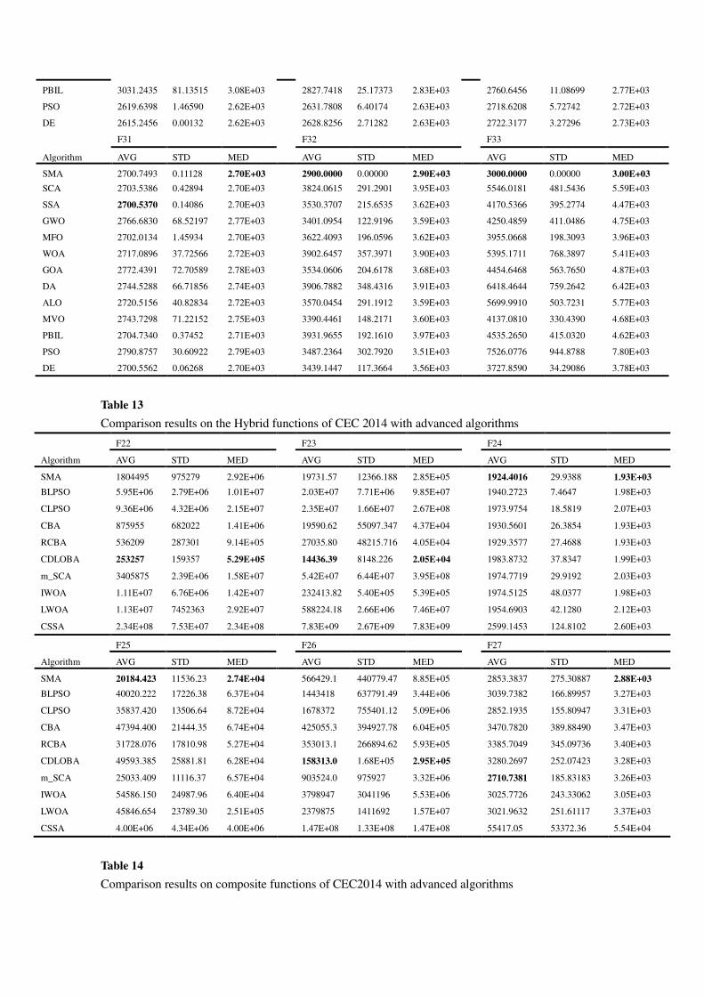
Tables 13-14 illustrate that SMA can also maintain certain advantages in composition functions

compared with the advanced algorithm, which further reflects that SMA can avert falling into local

optimum with fast convergence. F25, F32, and F33 in Figure 10 also intuitively incarnate the

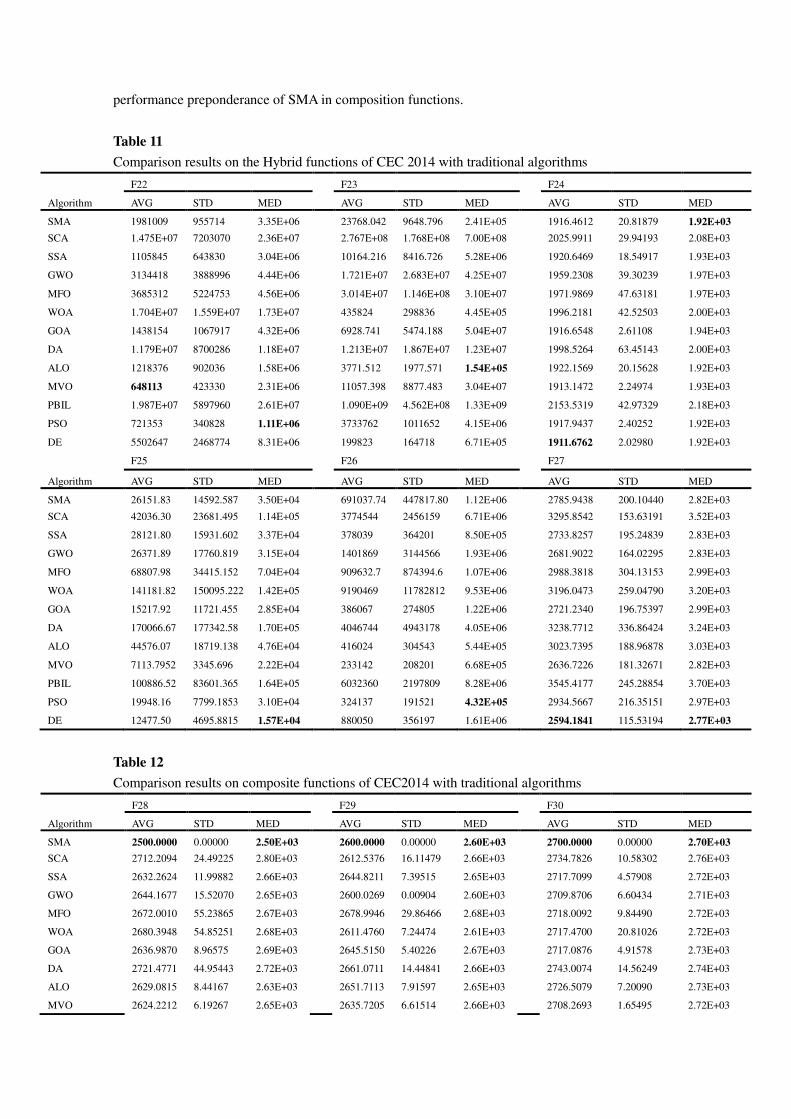
performance preponderance of SMA in composition functions.

Table 11

Comparison results on the Hybrid functions of CEC 2014 with traditional algorithms

F22 F23 F24


SMA 1981009 955714 3.35E+06 23768.042 9648.796 2.41E+05 1916.4612 20.81879 1.92E+03

SCA 1.475E+07 7203070 2.36E+07 2.767E+08 1.768E+08 7.00E+08 2025.9911 29.94193 2.08E+03

SSA 1105845 643830 3.04E+06 10164.216 8416.726 5.28E+06 1920.6469 18.54917 1.93E+03

GWO 3134418 3888996 4.44E+06 1.721E+07 2.683E+07 4.25E+07 1959.2308 39.30239 1.97E+03

MFO 3685312 5224753 4.56E+06 3.014E+07 1.146E+08 3.10E+07 1971.9869 47.63181 1.97E+03

WOA 1.704E+07 1.559E+07 1.73E+07 435824 298836 4.45E+05 1996.2181 42.52503 2.00E+03

GOA 1438154 1067917 4.32E+06 6928.741 5474.188 5.04E+07 1916.6548 2.61108 1.94E+03

DA 1.179E+07 8700286 1.18E+07 1.213E+07 1.867E+07 1.23E+07 1998.5264 63.45143 2.00E+03

ALO 1218376 902036 1.58E+06 3771.512 1977.571 1.54E+05 1922.1569 20.15628 1.92E+03

MVO 648113 423330 2.31E+06 11057.398 8877.483 3.04E+07 1913.1472 2.24974 1.93E+03

PBIL 1.987E+07 5897960 2.61E+07 1.090E+09 4.562E+08 1.33E+09 2153.5319 42.97329 2.18E+03

PSO 721353 340828 1.11E+06 3733762 1011652 4.15E+06 1917.9437 2.40252 1.92E+03

DE 5502647 2468774 8.31E+06 199823 164718 6.71E+05 1911.6762 2.02980 1.92E+03

F25 F26 F27


SMA 26151.83 14592.587 3.50E+04 691037.74 447817.80 1.12E+06 2785.9438 200.10440 2.82E+03

SCA 42036.30 23681.495 1.14E+05 3774544 2456159 6.71E+06 3295.8542 153.63191 3.52E+03

SSA 28121.80 15931.602 3.37E+04 378039 364201 8.50E+05 2733.8257 195.24839 2.83E+03

GWO 26371.89 17760.819 3.15E+04 1401869 3144566 1.93E+06 2681.9022 164.02295 2.83E+03

MFO 68807.98 34415.152 7.04E+04 909632.7 874394.6 1.07E+06 2988.3818 304.13153 2.99E+03

WOA 141181.82 150095.222 1.42E+05 9190469 11782812 9.53E+06 3196.0473 259.04790 3.20E+03

GOA 15217.92 11721.455 2.85E+04 386067 274805 1.22E+06 2721.2340 196.75397 2.99E+03

DA 170066.67 177342.58 1.70E+05 4046744 4943178 4.05E+06 3238.7712 336.86424 3.24E+03

ALO 44576.07 18719.138 4.76E+04 416024 304543 5.44E+05 3023.7395 188.96878 3.03E+03

MVO 7113.7952 3345.696 2.22E+04 233142 208201 6.68E+05 2636.7226 181.32671 2.82E+03

PBIL 100886.52 83601.365 1.64E+05 6032360 2197809 8.28E+06 3545.4177 245.28854 3.70E+03

PSO 19948.16 7799.1853 3.10E+04 324137 191521 4.32E+05 2934.5667 216.35151 2.97E+03

DE 12477.50 4695.8815 1.57E+04 880050 356197 1.61E+06 2594.1841 115.53194 2.77E+03

Table 12

Comparison results on composite functions of CEC2014 with traditional algorithms

F28 F29 F30


SMA 2500.0000 0.00000 2.50E+03 2600.0000 0.00000 2.60E+03 2700.0000 0.00000 2.70E+03

SCA 2712.2094 24.49225 2.80E+03 2612.5376 16.11479 2.66E+03 2734.7826 10.58302 2.76E+03

SSA 2632.2624 11.99882 2.66E+03 2644.8211 7.39515 2.65E+03 2717.7099 4.57908 2.72E+03

GWO 2644.1677 15.52070 2.65E+03 2600.0269 0.00904 2.60E+03 2709.8706 6.60434 2.71E+03

MFO 2672.0010 55.23865 2.67E+03 2678.9946 29.86466 2.68E+03 2718.0092 9.84490 2.72E+03

WOA 2680.3948 54.85251 2.68E+03 2611.4760 7.24474 2.61E+03 2717.4700 20.81026 2.72E+03

GOA 2636.9870 8.96575 2.69E+03 2645.5150 5.40226 2.67E+03 2717.0876 4.91578 2.73E+03

DA 2721.4771 44.95443 2.72E+03 2661.0711 14.44841 2.66E+03 2743.0074 14.56249 2.74E+03

ALO 2629.0815 8.44167 2.63E+03 2651.7113 7.91597 2.65E+03 2726.5079 7.20090 2.73E+03

MVO 2624.2212 6.19267 2.65E+03 2635.7205 6.61514 2.66E+03 2708.2693 1.65495 2.72E+03

PBIL 3031.2435 81.13515 3.08E+03 2827.7418 25.17373 2.83E+03 2760.6456 11.08699 2.77E+03

PSO 2619.6398 1.46590 2.62E+03 2631.7808 6.40174 2.63E+03 2718.6208 5.72742 2.72E+03

DE 2615.2456 0.00132 2.62E+03 2628.8256 2.71282 2.63E+03 2722.3177 3.27296 2.73E+03

F31 F32 F33


SMA 2700.7493 0.11128 2.70E+03 2900.0000 0.00000 2.90E+03 3000.0000 0.00000 3.00E+03

SCA 2703.5386 0.42894 2.70E+03 3824.0615 291.2901 3.95E+03 5546.0181 481.5436 5.59E+03

SSA 2700.5370 0.14086 2.70E+03 3530.3707 215.6535 3.62E+03 4170.5366 395.2774 4.47E+03

GWO 2766.6830 68.52197 2.77E+03 3401.0954 122.9196 3.59E+03 4250.4859 411.0486 4.75E+03

MFO 2702.0134 1.45934 2.70E+03 3622.4093 196.0596 3.62E+03 3955.0668 198.3093 3.96E+03

WOA 2717.0896 37.72566 2.72E+03 3902.6457 357.3971 3.90E+03 5395.1711 768.3897 5.41E+03

GOA 2772.4391 72.70589 2.78E+03 3534.0606 204.6178 3.68E+03 4454.6468 563.7650 4.87E+03

DA 2744.5288 66.71856 2.74E+03 3906.7882 348.4316 3.91E+03 6418.4644 759.2642 6.42E+03

ALO 2720.5156 40.82834 2.72E+03 3570.0454 291.1912 3.59E+03 5699.9910 503.7231 5.77E+03

MVO 2743.7298 71.22152 2.75E+03 3390.4461 148.2171 3.60E+03 4137.0810 330.4390 4.68E+03

PBIL 2704.7340 0.37452 2.71E+03 3931.9655 192.1610 3.97E+03 4535.2650 415.0320 4.62E+03

PSO 2790.8757 30.60922 2.79E+03 3487.2364 302.7920 3.51E+03 7526.0776 944.8788 7.80E+03

DE 2700.5562 0.06268 2.70E+03 3439.1447 117.3664 3.56E+03 3727.8590 34.29086 3.78E+03

Table 13

Comparison results on the Hybrid functions of CEC 2014 with advanced algorithms

F22 F23 F24


SMA 1804495 975279 2.92E+06 19731.57 12366.188 2.85E+05 1924.4016 29.9388 1.93E+03

BLPSO 5.95E+06 2.79E+06 1.01E+07 2.03E+07 7.71E+06 9.85E+07 1940.2723 7.4647 1.98E+03

CLPSO 9.36E+06 4.32E+06 2.15E+07 2.35E+07 1.66E+07 2.67E+08 1973.9754 18.5819 2.07E+03

CBA 875955 682022 1.41E+06 19590.62 55097.347 4.37E+04 1930.5601 26.3854 1.93E+03

RCBA 536209 287301 9.14E+05 27035.80 48215.716 4.05E+04 1929.3577 27.4688 1.93E+03

CDLOBA 253257 159357 5.29E+05 14436.39 8148.226 2.05E+04 1983.8732 37.8347 1.99E+03

m_SCA 3405875 2.39E+06 1.58E+07 5.42E+07 6.44E+07 3.95E+08 1974.7719 29.9192 2.03E+03

IWOA 1.11E+07 6.76E+06 1.42E+07 232413.82 5.40E+05 5.39E+05 1974.5125 48.0377 1.98E+03

LWOA 1.13E+07 7452363 2.92E+07 588224.18 2.66E+06 7.46E+07 1954.6903 42.1280 2.12E+03

CSSA 2.34E+08 7.53E+07 2.34E+08 7.83E+09 2.67E+09 7.83E+09 2599.1453 124.8102 2.60E+03

F25 F26 F27


SMA 20184.423 11536.23 2.74E+04 566429.1 440779.47 8.85E+05 2853.3837 275.30887 2.88E+03

BLPSO 40020.222 17226.38 6.37E+04 1443418 637791.49 3.44E+06 3039.7382 166.89957 3.27E+03

CLPSO 35837.420 13506.64 8.72E+04 1678372 755401.12 5.09E+06 2852.1935 155.80947 3.31E+03

CBA 47394.400 21444.35 6.74E+04 425055.3 394927.78 6.04E+05 3470.7820 389.88490 3.47E+03

RCBA 31728.076 17810.98 5.27E+04 353013.1 266894.62 5.93E+05 3385.7049 345.09736 3.40E+03

CDLOBA 49593.385 25881.81 6.28E+04 158313.0 1.68E+05 2.95E+05 3280.2697 252.07423 3.28E+03

m_SCA 25033.409 11116.37 6.57E+04 903524.0 975927 3.32E+06 2710.7381 185.83183 3.26E+03

IWOA 54586.150 24987.96 6.40E+04 3798947 3041196 5.53E+06 3025.7726 243.33062 3.05E+03

LWOA 45846.654 23789.30 2.51E+05 2379875 1411692 1.57E+07 3021.9632 251.61117 3.37E+03

CSSA 4.00E+06 4.34E+06 4.00E+06 1.47E+08 1.33E+08 1.47E+08 55417.05 53372.36 5.54E+04

Table 14

Comparison results on composite functions of CEC2014 with advanced algorithms

F28 F29 F30


SMA 2500.0000 0.00000 2.50E+03 2600.0000 0.00000 2.60E+03 2700.0000 0.00000 2.70E+03

BLPSO 2642.6104 5.72836 2.68E+03 2667.7295 2.33812 2.68E+03 2729.1590 3.76596 2.74E+03

CLPSO 2641.0387 6.17469 2.73E+03 2660.4964 3.06098 2.69E+03 2723.7881 4.81229 2.74E+03

CBA 2618.5576 2.10126 2.62E+03 2672.7287 32.2058 2.67E+03 2738.8447 16.6010 2.74E+03

RCBA 2616.5451 1.59102 2.62E+03 2671.7927 31.5474 2.67E+03 2734.0323 12.9174 2.73E+03

CDLOBA 2619.8273 5.91180 2.63E+03 2701.7423 41.3677 2.70E+03 2724.5749 12.1083 2.73E+03

m_SCA 2657.6041 18.7651 2.70E+03 2600.0082 0.00530 2.60E+03 2717.9183 3.76490 2.74E+03

IWOA 2653.0880 16.8268 2.66E+03 2607.2619 5.28645 2.61E+03 2714.2469 16.8627 2.72E+03

LWOA 2635.7620 26.8390 2.81E+03 2610.4768 6.01548 2.61E+03 2712.9723 16.0958 2.72E+03

CSSA 2525.7607 121.6063 2.53E+03 2600.4211 0.21279 2.60E+03 2700.0573 0.03311 2.70E+03

F31 F32 F33


SMA 2700.7690 0.14584 2.70E+03 2900.0000 0.000000 2.90E+03 3000.0000 0.000000 3.03E+03

BLPSO 2719.8189 40.7556 2.73E+03 3639.7610 104.8236 3.78E+03 4689.9702 351.2075 5.46E+03

CLPSO 2703.1872 0.86410 2.71E+03 3255.3722 59.2992 3.45E+03 5394.7830 503.6760 6.86E+03

CBA 2714.7665 60.7392 2.72E+03 3992.4341 466.0520 4.00E+03 5749.7099 1087.8530 5.77E+03

RCBA 2731.0975 67.5372 2.75E+03 4088.5512 406.7701 4.11E+03 5820.2491 1076.0463 5.86E+03

CDLOBA 2715.7761 56.3032 2.72E+03 3902.9353 371.3979 3.91E+03 5346.9885 837.0278 5.36E+03

m_SCA 2701.3185 0.81232 2.70E+03 3324.8813 254.9219 3.52E+03 4280.9832 270.1009 4.87E+03

IWOA 2732.9019 77.0976 2.73E+03 3800.5003 342.5802 3.83E+03 5181.1074 676.4584 5.28E+03

LWOA 2700.5873 0.13596 2.70E+03 3865.9583 237.8645 4.00E+03 4457.1988 270.3753 4.91E+03

CSSA 2792.4644 23.3249 2.79E+03 4836.8934 344.1577 4.84E+03 8555.0615 3476.6646 8.56E+03

Figure 9 Comparisons between SMA and traditional MAs

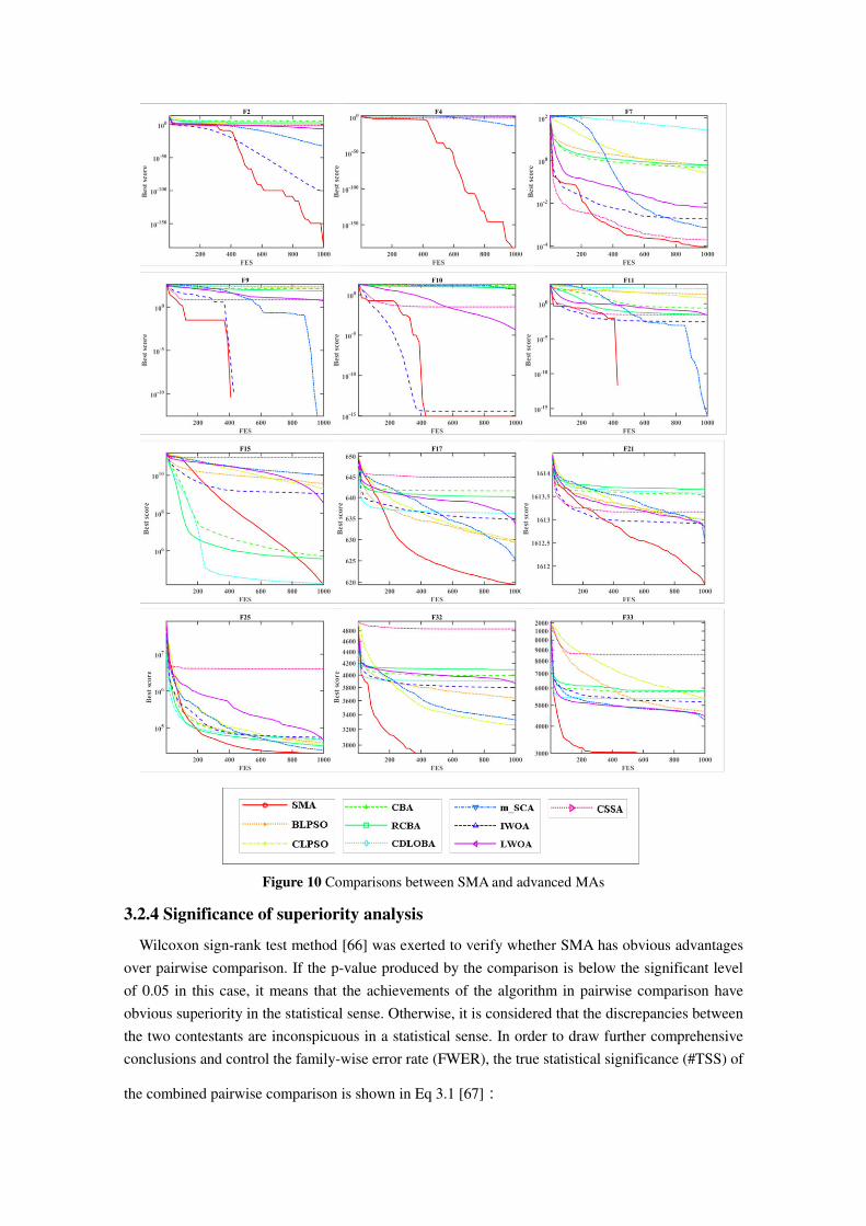
Figure 10 Comparisons between SMA and advanced MAs

3.2.4 Significance of superiority analysis

Wilcoxon sign-rank test method [66] was exerted to verify whether SMA has obvious advantages

over pairwise comparison. If the p-value produced by the comparison is below the significant level

of 0.05 in this case, it means that the achievements of the algorithm in pairwise comparison have

obvious superiority in the statistical sense. Otherwise, it is considered that the discrepancies between

the two contestants are inconspicuous in a statistical sense. In order to draw further comprehensive

conclusions and control the family-wise error rate (FWER), the true statistical significance (#TSS) of

the combined pairwise comparison is shown in Eq 3.1 [67]：

𝑝 = 1 −∏ 1− 𝑝𝐻1𝑘 𝑖 (3.1)

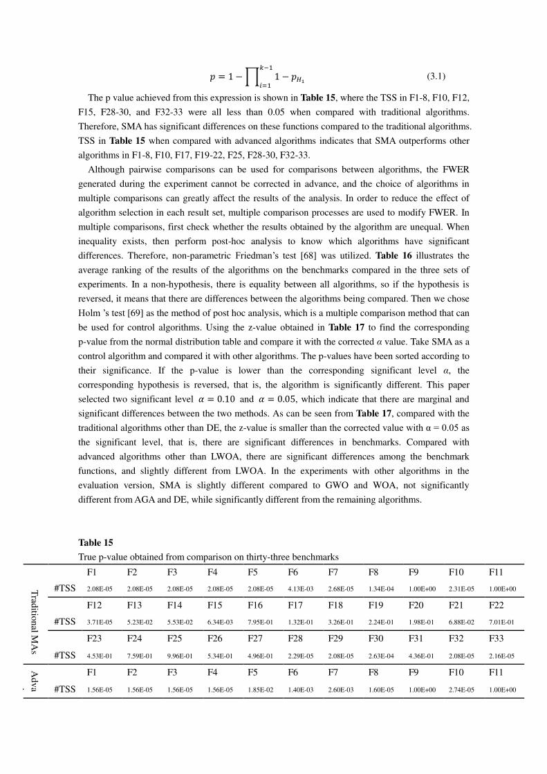
The p value achieved from this expression is shown in Table 15, where the TSS in F1-8, F10, F12,

F15, F28-30, and F32-33 were all less than 0.05 when compared with traditional algorithms.

Therefore, SMA has significant differences on these functions compared to the traditional algorithms.

TSS in Table 15 when compared with advanced algorithms indicates that SMA outperforms other

algorithms in F1-8, F10, F17, F19-22, F25, F28-30, F32-33.

Although pairwise comparisons can be used for comparisons between algorithms, the FWER

generated during the experiment cannot be corrected in advance, and the choice of algorithms in

multiple comparisons can greatly affect the results of the analysis. In order to reduce the effect of

algorithm selection in each result set, multiple comparison processes are used to modify FWER. In

multiple comparisons, first check whether the results obtained by the algorithm are unequal. When

inequality exists, then perform post-hoc analysis to know which algorithms have significant

differences. Therefore, non-parametric Friedman’s test [68] was utilized. Table 16 illustrates the

average ranking of the results of the algorithms on the benchmarks compared in the three sets of

experiments. In a non-hypothesis, there is equality between all algorithms, so if the hypothesis is

reversed, it means that there are differences between the algorithms being compared. Then we chose

Holm ’s test [69] as the method of post hoc analysis, which is a multiple comparison method that can

be used for control algorithms. Using the z-value obtained in Table 17 to find the corresponding

p-value from the normal distribution table and compare it with the corrected α value. Take SMA as a

control algorithm and compared it with other algorithms. The p-values have been sorted according to

their significance. If the p-value is lower than the corresponding significant level α, the

corresponding hypothesis is reversed, that is, the algorithm is significantly different. This paper

selected two significant level 𝛼 = 0.10 and 𝛼 = 0.05, which indicate that there are marginal and

significant differences between the two methods. As can be seen from Table 17, compared with the

traditional algorithms other than DE, the z-value is smaller than the corrected value with α = 0.05 as the significant level, that is, there are significant differences in benchmarks. Compared with

advanced algorithms other than LWOA, there are significant differences among the benchmark

functions, and slightly different from LWOA. In the experiments with other algorithms in the

evaluation version, SMA is slightly different compared to GWO and WOA, not significantly

different from AGA and DE, while significantly different from the remaining algorithms.

Table 15

True p-value obtained from comparison on thirty-three benchmarks

F1 F2 F3 F4 F5 F6 F7 F8 F9 F10 F11

Trad

ition

al MA

s

#TSS 2.08E-05 2.08E-05 2.08E-05 2.08E-05 2.08E-05 4.13E-03 2.68E-05 1.34E-04 1.00E+00 2.31E-05 1.00E+00

F12 F13 F14 F15 F16 F17 F18 F19 F20 F21 F22

#TSS 3.71E-05 5.23E-02 5.53E-02 6.34E-03 7.95E-01 1.32E-01 3.26E-01 2.24E-01 1.98E-01 6.88E-02 7.01E-01

F23 F24 F25 F26 F27 F28 F29 F30 F31 F32 F33

#TSS 4.53E-01 7.59E-01 9.96E-01 5.34E-01 4.96E-01 2.29E-05 2.08E-05 2.63E-04 4.36E-01 2.08E-05 2.16E-05

Adva

nced

F1 F2 F3 F4 F5 F6 F7 F8 F9 F10 F11

#TSS 1.56E-05 1.56E-05 1.56E-05 1.56E-05 1.85E-02 1.40E-03 2.60E-03 1.60E-05 1.00E+00 2.74E-05 1.00E+00

F12 F13 F14 F15 F16 F17 F18 F19 F20 F21 F22

#TSS 1.83E-01 4.91E-01 1.25E-01 1.91E-01 9.93E-01 1.86E-05 7.57E-01 5.59E-04 1.56E-05 3.22E-05 2.04E-03

F23 F24 F25 F26 F27 F28 F29 F30 F31 F32 F33

#TSS 3.37E-01 5.58E-02 3.91E-02 3.62E-01 8.15E-01 1.56E-05 1.56E-05 7.49E-05 7.75E-01 1.56E-05 1.64E-05

Table 166

Results of Friedman test of iterative version and function evaluation version

Iterative version on F1-33

SMA SCA SSA GWO MFO WOA GOA DA ALO MVO PBIL PSO DE

Avg 3.057 9.396 5.180 5.280 8.037 6.735 6.690 10.580 6.124 5.013 12.228 7.865 4.815

Rank 1 11 4 5 10 8 7 12 6 3 13 9 2

Iterative version on F1-33

SMA BLPS CLPS CBA RCBA CDLO m_SC IWOA LWOA CSSA

Avg 2.297 7.578 6.996 5.507 5.408 6.100 5.000 4.710 4.907 6.497

Rank 1 10 9 6 5 7 4 2 3 8

Evaluation version on F1-21

SMA SCA SSA GWO MFO WOA GOA MVO PSO DE AGA

Avg 3.189 8.103 5.668 5.369 8.201 5.135 6.805 5.895 8.970 4.292 4.373

Rank 1 9 6 5 10 4 8 7 11 2 3

Table 177

Holms’ test (take SMA as the control algorithm)

𝑆𝑀𝐴 𝑉𝑆. 𝑧 − 𝑣𝑎𝑙𝑢𝑒 𝑝 − 𝑣𝑎𝑙𝑢𝑒 𝛼/𝑖 , 𝛼 = 0.05 𝛼/𝑖, 𝛼 = 0.10

Trad

itional alg

orith

ms

PBIL 9.9878 8.6010E-24 0.0042 0.0083

DA 8.2494 7.9860E-17 0.0045 0.0091

SCA 6.9851 1.4240E-12 0.005 0.01

MFO 6.7639 6.7120E-12 0.0056 0.0111

PSO 4.9307 4.0900E-07 0.0063 0.0125

WOA 4.2669 9.9060E-06 0.0071 0.0143

GOA 3.8877 5.0540E-05 0.0083 0.0167

ALO 3.7296 9.5740E-05 0.01 0.02

GWO 2.9394 1.6460E-03 0.0125 0.025

SSA 2.3389 9.6680E-03 0.0167 0.0333

MVO 1.7384 0.04111 0.025 0.05

DE 1.6436 0.05009 0.05 0.1

Ad

van

ced alg

orith

ms

BLPSO 12.0748 7.1760E-34 0.00556 0.01111

CLPSO 10.7331 3.5580E-27 0.00625 0.0125

CSSA 9.3915 2.9580E-21 0.00714 0.01429

CDLOBA 8.0498 4.1460E-16 0.00833 0.01667

CBA 6.7082 9.8520E-12 0.01 0.02

RCBA 5.3666 4.0120E-08 0.0125 0.025

IWOA 4.0249 2.8500E-05 0.01667 0.03333

m_SCA 2.6833 0.00365 0.025 0.05

LWOA 1.3416 0.08986 0.05 0.1

Ev

aluatio

n

PSO 5.648039 8.1160E-09 0.005 0.01

MFO 4.896673 4.8730E-07 0.0056 0.0111

SCA 4.801299 7.8820E-07 0.00625 0.0125

GOA 3.532738 2.0570E-04 0.0071 0.0143

MVO 2.644126 0.0041 0.0083 0.0167

SSA 2.422361 0.0077 0.01 0.02

GWO 2.130033 0.0166 0.0125 0.025

WOA 1.901289 0.0286 0.0167 0.0333

AGA 1.156902 0.1237 0.025 0.05

DE 1.077811 0.1406 0.05 0.1

3.3 Wall-clock time analysis

In this section of the experimentations, SMA was compared with other 11 participants in the

calculation of time-consuming experiments in the 33 benchmarks mentioned above. The

time-consuming calculation approach is that all participants independently run 10 times on each

function and recorded the results in Table 18. As can be observed from the data in the table, the

computation of SMA took relatively longer time, because the calculation of the oscillation factor

requires more computing power. However, SMA can still outperform some algorithms while taking

less time, such as GOA, DA, and ALO. In general, even if it is relatively time-consuming, SMA still

possess tremendous effectiveness advantages over other algorithms, so the time-consuming is worth

it.

Table 18

Wall-Clock Time costs of SMA and other candidates on 33 benchmarks

SMA SCA SSA GWO MFO WOA GOA DA ALO MVO PSO DE

F1 14.040 1.310 0.811 1.825 1.513 0.562 119.46 90.262 218.35 3.822 0.967 5.054

F2 13.291 1.139 0.796 1.622 1.342 0.577 118.10 110.88 216.74 3.806 0.920 4.446

F3 13.478 2.480 2.215 2.839 2.636 2.278 110.01 116.26 207.60 4.165 1.919 5.288

F4 12.776 1.123 0.796 1.560 1.123 0.546 117.18 86.659 207.51 2.761 0.640 3.838

F5 12.995 1.404 1.030 1.950 1.466 0.780 123.64 115.76 233.11 3.401 0.874 4.976

F6 15.241 1.513 1.045 2.090 1.544 0.686 146.37 122.92 260.16 3.760 0.889 4.914

F7 16.037 2.356 1.919 2.855 2.465 1.638 141.66 118.85 257.99 4.883 1.794 5.678

F8 15.709 1.763 1.295 2.434 1.778 0.983 141.11 172.03 255.46 2.824 1.264 5.491

F9 16.115 1.576 1.123 2.028 1.669 0.764 142.13 136.65 259.30 3.994 1.139 4.742

F10 14.726 1.794 1.279 2.090 1.997 0.936 143.20 111.15 251.09 4.025 1.092 5.444

F11 16.115 2.215 1.607 2.309 1.981 0.998 144.87 121.33 264.06 4.040 1.217 5.600

F12 19.032 4.602 4.134 5.023 4.836 3.900 149.91 124.59 265.56 6.880 4.134 8.596

F13 18.939 4.852 4.274 5.101 4.243 3.604 149.15 126.20 266.68 6.833 4.087 8.518

F14 16.411 2.090 1.732 2.855 2.340 1.326 140.80 145.54 256.34 4.399 1.544 5.647

F15 15.725 2.106 1.498 2.465 1.950 1.108 144.89 136.08 261.58 4.524 1.373 5.990

F16 15.803 2.106 1.638 2.652 2.044 1.295 146.76 152.35 261.16 4.243 1.342 5.351

F17 31.715 16.677 15.943 17.254 16.224 15.678 163.83 185.08 281.14 19.438 16.021 20.686

F18 16.177 2.090 1.544 2.621 2.246 1.279 146.37 170.30 263.08 4.508 1.342 5.288

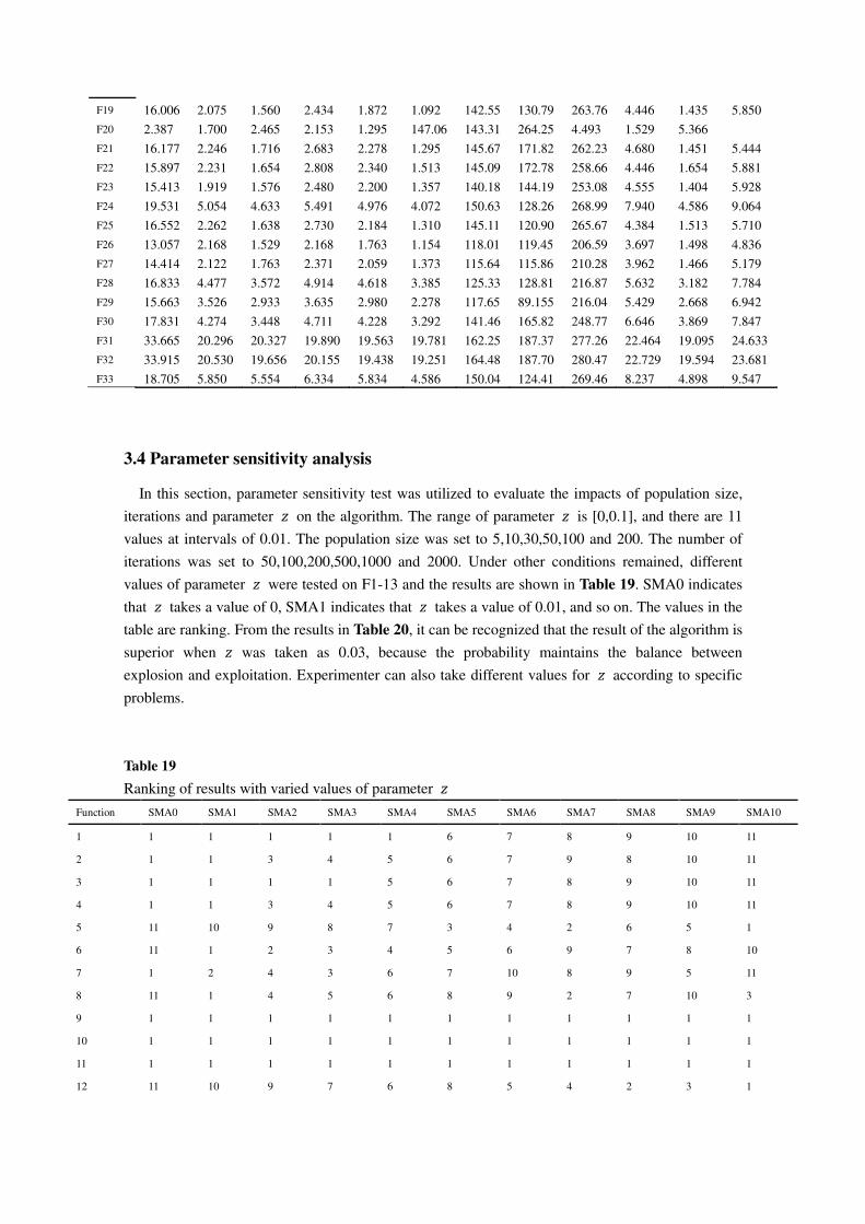
F19 16.006 2.075 1.560 2.434 1.872 1.092 142.55 130.79 263.76 4.446 1.435 5.850

F20 2.387 1.700 2.465 2.153 1.295 147.06 143.31 264.25 4.493 1.529 5.366

F21 16.177 2.246 1.716 2.683 2.278 1.295 145.67 171.82 262.23 4.680 1.451 5.444

F22 15.897 2.231 1.654 2.808 2.340 1.513 145.09 172.78 258.66 4.446 1.654 5.881

F23 15.413 1.919 1.576 2.480 2.200 1.357 140.18 144.19 253.08 4.555 1.404 5.928

F24 19.531 5.054 4.633 5.491 4.976 4.072 150.63 128.26 268.99 7.940 4.586 9.064

F25 16.552 2.262 1.638 2.730 2.184 1.310 145.11 120.90 265.67 4.384 1.513 5.710

F26 13.057 2.168 1.529 2.168 1.763 1.154 118.01 119.45 206.59 3.697 1.498 4.836

F27 14.414 2.122 1.763 2.371 2.059 1.373 115.64 115.86 210.28 3.962 1.466 5.179

F28 16.833 4.477 3.572 4.914 4.618 3.385 125.33 128.81 216.87 5.632 3.182 7.784

F29 15.663 3.526 2.933 3.635 2.980 2.278 117.65 89.155 216.04 5.429 2.668 6.942

F30 17.831 4.274 3.448 4.711 4.228 3.292 141.46 165.82 248.77 6.646 3.869 7.847

F31 33.665 20.296 20.327 19.890 19.563 19.781 162.25 187.37 277.26 22.464 19.095 24.633

F32 33.915 20.530 19.656 20.155 19.438 19.251 164.48 187.70 280.47 22.729 19.594 23.681

F33 18.705 5.850 5.554 6.334 5.834 4.586 150.04 124.41 269.46 8.237 4.898 9.547

3.4 Parameter sensitivity analysis

In this section, parameter sensitivity test was utilized to evaluate the impacts of population size,

iterations and parameter 𝑧 on the algorithm. The range of parameter 𝑧 is [0,0.1], and there are 11

values at intervals of 0.01. The population size was set to 5,10,30,50,100 and 200. The number of

iterations was set to 50,100,200,500,1000 and 2000. Under other conditions remained, different

values of parameter 𝑧 were tested on F1-13 and the results are shown in Table 19. SMA0 indicates

that 𝑧 takes a value of 0, SMA1 indicates that 𝑧 takes a value of 0.01, and so on. The values in the

table are ranking. From the results in Table 20, it can be recognized that the result of the algorithm is

superior when 𝑧 was taken as 0.03, because the probability maintains the balance between

explosion and exploitation. Experimenter can also take different values for 𝑧 according to specific

problems.

Table 19

Ranking of results with varied values of parameter 𝑧

Function SMA0 SMA1 SMA2 SMA3 SMA4 SMA5 SMA6 SMA7 SMA8 SMA9 SMA10

1 1 1 1 1 1 6 7 8 9 10 11

2 1 1 3 4 5 6 7 9 8 10 11

3 1 1 1 1 5 6 7 8 9 10 11

4 1 1 3 4 5 6 7 8 9 10 11

5 11 10 9 8 7 3 4 2 6 5 1

6 11 1 2 3 4 5 6 9 7 8 10

7 1 2 4 3 6 7 10 8 9 5 11

8 11 1 4 5 6 8 9 2 7 10 3

9 1 1 1 1 1 1 1 1 1 1 1

10 1 1 1 1 1 1 1 1 1 1 1

11 1 1 1 1 1 1 1 1 1 1 1

12 11 10 9 7 6 8 5 4 2 3 1

13 11 10 2 1 8 4 5 3 9 7 6

Average 4.85E+00 3.15E+00 3.15E+00 3.08E+00 4.31E+00 4.77E+00 5.38E+00 4.92E+00 6.00E+00 6.23E+00 6.08E+00

Rank 5 2 2 1 3 4 7 6 8 10 9

To explore the influence of populations and iterations on the algorithm, we chose F13 to test the

synergistic effect of the two parameters on the algorithm. As can be seen visually from Figure 11, as

the population size and iterations increased, the average became better. The reason is that the

increase in the number of populations improves the search efficiency, and the increase in iterations

leads to an incensement in the times of searches and the accuracy of subsequent searches. However,

the results were not increased proportionally when the population size and iterations continue to

grow due to the global approximate optimal solution has been roughly discovered. Researchers can

select the appropriate populations and iterations based on specific questions.

Figure 11 The influence of populations and iterations

3.5 Experiments on engineering design problems

Most problems have constraints in the real production environment. The process of considering

constraints of equality and inequality during optimization is called constraints processing. The

candidate solutions of the heuristic algorithm can be divided into feasible and infeasible according to

the constraints. There are currently several types of constraint methods: death penalty, annealing,

static, dynamic, co-evolutionary, and adaptive. Although useful information may be lost in the

process of abandonment, we still adopted a relatively simple method of the death penalty with low

computational cost to deal with search individuals who violated constraints and then re-assigned

them a relatively large target value.

In the following sections, SMA is tested four engineering-constrained design problems: a welded

beam problem, a pressure vessel problem, a cantilever, and I-beam.

3.5.1 Welded beam structure problem

The main purpose of the problem is to constrain side constraints, end deflection of the beam(𝛿), buckling load on the bar( 𝑐), bending stress in the beam( ), moreover, shear stress( ) with the least

economic cost of welded beams.

There are four variables, for instance, the thickness of the weld(𝑕), length of the attached bar(𝑙), the height of the bar(𝑡), the thickness of the bar(𝑏). The design diagram for this problem is shown in

Figure 12. The formulations were list below:

Consider: 𝑋 = ,𝑥 , 𝑥 , 𝑥 , 𝑥 - = ,𝑕 𝑙 𝑡 𝑏- Minimize: 𝐹(𝑋) = 1.10471𝑥 𝑥 + 0.04811𝑥 𝑥 (14.0 + 𝑥 ) Subject to: 𝑔 (𝑋) = (𝑋) − 𝑚𝑎 ≤ 0 𝑔 (𝑋) = 𝜎(𝑋) − 𝜎𝑚𝑎 ≤ 0 𝑔 (𝑋) = 𝛿(𝑋) − 𝛿𝑚𝑎 ≤ 0 𝑔 (𝑋) = 𝑥 − 𝑥 ≤ 0 𝑔 (𝑋) = − 𝐶(𝑋) ≤ 0 𝑔 (𝑋) = 0.125 − 𝑥 ≤ 0 𝑔 (𝑋) = 1.10471𝑥 + 0.04811𝑥 𝑥 (14.0 + 𝑥 ) − 5.0 ≤ 0

where τ(𝑥 ) = √( ′) + 2 ′ ′′ 𝑥 2𝑅 + ( ′′) ′ = √2𝑥 𝑥 , ′′ = 𝑀𝑅𝐽 ,M = P(L + 𝑥 2 ) = √𝑥 4 + (𝑥 + 𝑥 2 )

𝐽 = 2 ,√2𝑥 𝑥 *𝑥 4 + (𝑥 + 𝑥 2 ) +- σ(𝑥 ) = 6 𝐿𝑥 𝑥 , δ(𝑥 ) = 6 𝐿 𝐸𝑥 𝑥

𝐶(𝑥 ) = 4.013𝐸√𝑥 𝑥 36𝐿 (1 − 𝑥 2𝐿√ 𝐸4𝐺) P = 60001 , L = 14 n. . 𝛿𝑚𝑎 = 0.25 𝑖𝑛. = 30 × 1 𝑝𝑠𝑖, = 12 × 10 𝑝𝑠𝑖 𝑚𝑎 = 13600𝑝𝑠𝑖, 𝜎𝑚𝑎 = 30000𝑝𝑠𝑖 In this problem, SMA was compared with MFO[23], SSA[52], Random[70], Siddall[71],

Ragsdell[70], Coello and Montes[72], GWO[21], WOA[50], GSA, Simplex[70] and David[70].

Table 20 illustrates that SMA can obtain the optimal value.

I

h

t

L

P

b

Figure 12 Structure of welded beam design

Table 20

Results of welded beam structure problem compared with other competitors

Algorithms Optimum values for variables Optimum

cost h l t b

SMA 0.2054 3.2589 9.0384 0.2058 1.69604

MFO[23] 0.2057 3.4703 9.0364 0.2057 1.72452

SSA[52] 0.2057 3.4714 9.0366 0.2057 1.72491

Random[70] 0.4575 4.7313 5.0853 0.6600 4.11856

Siddall[71] 0.2444 6.2189 8.2915 0.2444 2.38154

Ragsdell[70] 0.2455 6.1960 8.2730 0.2455 2.38594

Coello and

Montes[72] 0.2060 3.4713 9.0202 0.2065 1.72822

GWO[21] 0.2057 3.4784 9.0368 0.2058 1.72624

WOA[50] 0.2054 3.4843 9.0374 0.2063 1.73050

GSA 0.1821 3.8570 10.0000 0.2024 1.87995

Simplex[70] 0.2792 5.6256 7.7512 0.2796 2.53073

David[70] 0.2434 6.2552 8.2915 0.2444 2.38411

3.5.2 Pressure vessel structure problem

The intention of the problem is to find the parameters of cylindrical pressure vessels which can

minimize the total cost of production and meet the pressure requirements. The parameters including

the thickness of the shell(𝑇𝑠), inner radius(𝑇ℎ), the thickness of the head(𝑇ℎ) and the length of the

cylindrical portion. Both ends of the container are covered with a hemispherical shell at one end.

Figure 13 illustrates the design of the object and its corresponding parameters.

The formulations of four constraints are listed as follow:

Consider: 𝑋 = ,𝑥 𝑥 𝑥 𝑥 - = ,𝑇𝑠 𝑇ℎ 𝑅 𝐿- Objective: 𝑓(𝑋)𝑚𝑖𝑛 = 0.6224𝑥 𝑥 𝑥 + 1.7781𝑥 𝑥 + 3.1661𝑥 𝑥 + 19.84𝑥 𝑥 Subject to: 𝑔 (𝑋) = −𝑥 + 0.0193𝑥 ≤ 0

𝑔 (𝑋) = −𝑥 + 0.00954𝑥 ≤ 0 𝑔 (𝑋) = − 𝑥 𝑥 − 43 𝑥 + 1296000 ≤ 0 𝑔 (𝑋) = 𝑥 − 240 ≤ 0

Variable ranges: 0 ≤ 𝑥 ≤ 99, 0 ≤ 𝑥 ≤ 99, 10 ≤ 𝑥 ≤ 200, 10 ≤ 𝑥 ≤ 200

From the data of Table 21, it is obvious that SMA can obtain fairly superior optimal values

compared with MFO[23], BA[73], HPSO[74], CSS[5], CPSO[75], ACO[76], GWO[21], WOA[50],

MDDE[77], Lagrangian multiplier[78] and Branch-bound[79].

2R

L

ThTs

Figure 13 Structure of pressure vessel

Table 21

Results of pressure vessel design problem compared with other competitors

Algorithms Optimum values for variables

Optimum cost 𝑇𝑠 𝑇ℎ R L

SMA 0.7931 0.3932 40.6711 196.2178 5994.1857

MFO[23] 0.8125 0.4375 42.0984 176.6366 6059.7143

BA[73] 0.8125 0.4375 42.0984 176.6366 6059.7143

HPSO[74] 0.8125 0.4375 42.0984 176.6366 6059.7143

CSS[5] 0.8125 0.4375 42.1036 176.5727 6059.0888

CPSO[75] 0.8125 0.4375 42.0912 176.7465 6061.0777

ACO[76] 0.8125 0.4375 42.1036 176.5727 6059.0888

GWO[21] 0.8125 0.4345 42.0892 176.7587 6051.5639

WOA[50] 0.8125 0.4375 42.0983 176.6390 6059.7410

MDDE[77] 0.8125 0.4375 42.0984 176.6360 6059.7017

Lagrangian

multiplier[78] 1.1250 0.6250 58.2910 43.6900 7198.0428

Branch-bound

[79] 1.1250 0.6250 47.7000 117.7010 8129.1036

3.5.3 Cantilever structure problem

The cantilever beam is made up of five hollow square cross-sections, as exhibited in Figure 14.

Since the thickness is fixed, only six parameters identified in the figure need to be considered. The

intention of the problem is to dwindle the total mass of the cantilever beam when the bearing

capacity is satisfied. The formulas of this optimization problem are listed as follow:

Consider: 𝑋 = ,𝑥 𝑥 𝑥 𝑥 𝑥 - Minimize: 𝐹(𝑋) = 0.6224(𝑥 + 𝑥 + 𝑥 + 𝑥 + 𝑥 ) Subject to: (X) = 61x + 37𝑥 + 19𝑥 + 7𝑥 + 1𝑥 ≤ 1

Variable ranges: 0.01 ≤ x . 𝑥 , 𝑥 , 𝑥 , 𝑥 ≤ 100

constant

X

X

2341

56

Figure 14 Structure of cantilever beam

Compared to MFO[23], SOS[80], CS[81], MMA[82] and GCA[82], SMA can achieve better

results in the cantilever design problem, as shown in Table 22.

Table 22

Results of cantilever beam structural problem in comparison with other competitors

Algorithm Optimum values for variables Optimum

cost 𝑋 𝑋 𝑋 𝑋 𝑋 SMA 6.017757 5.310892 4.493758 3.501106 2.150159 1.339957

MFO[23] 5.9830 5.3167 4.4973 3.5136 2.1616 1.33998

SOS[80] 6.0188 5.3034 4.4959 3.4990 2.1556 1.33996

CS[81] 6.0089 5.3049 4.5023 3.5077 2.1504 1.33999

MMA[82] 6.0100 5.3000 4.4900 3.4900 2.1500 1.3400

GCA[82] 6.0100 5.3000 4.4900 3.4900 2.1500 1.3400

3.5.4 I-beam structure problem

The intention of this engineering problem is to minimize the vertical deviation of I-beam by

adjusting four parameters as shown in Figure 15.

b

P

Qh

tftwL

Figure 15 Structure of I-beam

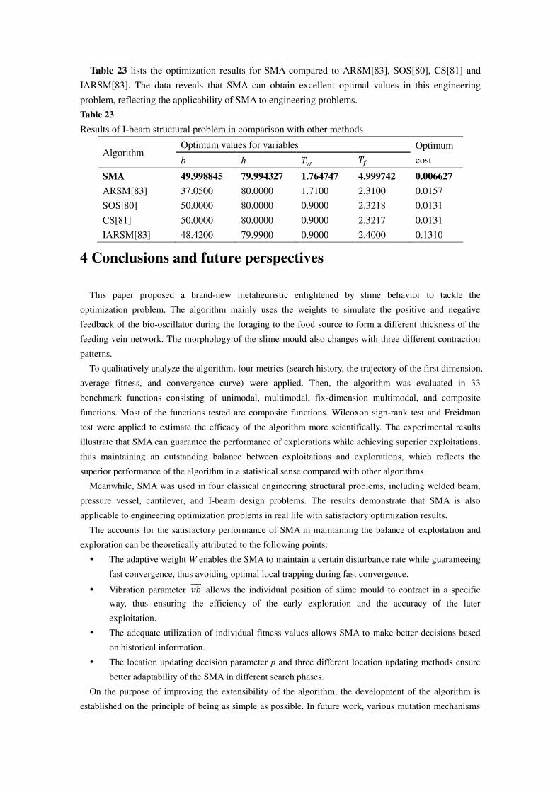
Table 23 lists the optimization results for SMA compared to ARSM[83], SOS[80], CS[81] and

IARSM[83]. The data reveals that SMA can obtain excellent optimal values in this engineering

problem, reflecting the applicability of SMA to engineering problems.

Table 23

Results of I-beam structural problem in comparison with other methods

Algorithm Optimum values for variables Optimum

cost b h 𝑇 𝑇

SMA 49.998845 79.994327 1.764747 4.999742 0.006627

ARSM[83] 37.0500 80.0000 1.7100 2.3100 0.0157

SOS[80] 50.0000 80.0000 0.9000 2.3218 0.0131

CS[81] 50.0000 80.0000 0.9000 2.3217 0.0131

IARSM[83] 48.4200 79.9900 0.9000 2.4000 0.1310

4 Conclusions and future perspectives

This paper proposed a brand-new metaheuristic enlightened by slime behavior to tackle the

optimization problem. The algorithm mainly uses the weights to simulate the positive and negative

feedback of the bio-oscillator during the foraging to the food source to form a different thickness of the

feeding vein network. The morphology of the slime mould also changes with three different contraction

patterns.

To qualitatively analyze the algorithm, four metrics (search history, the trajectory of the first dimension,

average fitness, and convergence curve) were applied. Then, the algorithm was evaluated in 33

benchmark functions consisting of unimodal, multimodal, fix-dimension multimodal, and composite

functions. Most of the functions tested are composite functions. Wilcoxon sign-rank test and Freidman

test were applied to estimate the efficacy of the algorithm more scientifically. The experimental results

illustrate that SMA can guarantee the performance of explorations while achieving superior exploitations,

thus maintaining an outstanding balance between exploitations and explorations, which reflects the

superior performance of the algorithm in a statistical sense compared with other algorithms.

Meanwhile, SMA was used in four classical engineering structural problems, including welded beam,

pressure vessel, cantilever, and I-beam design problems. The results demonstrate that SMA is also

applicable to engineering optimization problems in real life with satisfactory optimization results.

The accounts for the satisfactory performance of SMA in maintaining the balance of exploitation and

exploration can be theoretically attributed to the following points:

The adaptive weight W enables the SMA to maintain a certain disturbance rate while guaranteeing

fast convergence, thus avoiding optimal local trapping during fast convergence.

Vibration parameter 𝑣𝑏⃗⃗⃗⃗ allows the individual position of slime mould to contract in a specific

way, thus ensuring the efficiency of the early exploration and the accuracy of the later

exploitation.

The adequate utilization of individual fitness values allows SMA to make better decisions based

on historical information.

The location updating decision parameter p and three different location updating methods ensure

better adaptability of the SMA in different search phases.

On the purpose of improving the extensibility of the algorithm, the development of the algorithm is

established on the principle of being as simple as possible. In future work, various mutation mechanisms

or acceleration mechanisms can be employed to enhance the efficacy of the algorithm. The binary version

of the algorithm can also be developed for feature selection. Moreover, SMA can also be used to optimize

parameters of classifiers such as kernel extreme learning machine or support vector machine.

Acknowledgment

This research is supported by the Science and Technology Plan Project of Wenzhou, China

(2018ZG012), and the National Natural Science Foundation of China (U1809209).

References

1. Faris, H., et al., An intelligent system for spam detection and identification of the most relevant

features based on evolutionary Random Weight Networks. Information Fusion, 2019. 48: p.

67-83.

2. Osher, S., et al., Laplacian Smoothing Gradient Descent. 2018.

3. Mirjalili, S., S.M. Mirjalili, and A. Hatamlou, Multi-Verse Optimizer: a nature-inspired

algorithm for global optimization. Neural Computing and Applications, 2016. 27(2): p. 495-513.

4. Webster, B. and P. Bernhard, A Local Search Optimization Algorithm Based on Natural

Principles of Gravitation. 2003. 255-261.

5. Kaveh, A. and S. Talatahari, Talatahari, S.: A Novel Heuristic Optimization Method: Charged

System Search. Acta Mechanica 213(3-4), 267-289. Vol. 213. 2010. 267-289.

6. Rashedi, E., H. Nezamabadi-pour, and S. Saryazdi, GSA: a Gravitational Search Algorithm. Vol.

179. 2009. 2232-2248.

7. Mirjalili, S., SCA: A Sine Cosine Algorithm for solving optimization problems.

Knowledge-Based Systems, 2016. 96: p. 120-133.

8. Kirkpatrick, S., C.D. Gelatt Jr, and M.P. Vecchi, Optimization by simulated annealing. Science,

1983. 220(4598): p. 671-680.

9. Venkata Rao, R., V. Savsani, and D. P. Vakharia, Teaching–Learning-Based Optimization: An

optimization method for continuous non-linear large scale problems. Vol. 183. 2012. 1-15.

10. Formato, R., Central force optimization: A new metaheuristic with applications in applied

electromagnetics. Vol. 77. 2007. 425-491.

11. Fogel, D., Artificial Intelligence through Simulated Evolution. 2009. 227-296.

12. Booker, L.B., D.E. Goldberg, and J.H. Holland, Classifier systems and genetic algorithms.

Artificial Intelligence, 1989. 40(1): p. 235-282.

13. Koza, J.R. and J.P. Rice. Automatic programming of robots using genetic programming. in

Proceedings Tenth National Conference on Artificial Intelligence. 1992.

14. Hansen, N., S. D Müller, and P. Koumoutsakos, Reducing the Time Complexity of the

Derandomized Evolution Strategy with Covariance Matrix Adaptation (CMA-ES). Vol. 11. 2003.

1-18.

15. Yao, X., Y. Liu, and G. Lin, Evolutionary Programming Made Faster. Vol. 3. 1999. 82-102.

16. Storn, R. and K. Price, Differential Evolution - A Simple and Efficient Heuristic for Global

Optimization over Continuous Spaces. Vol. 11. 1997. 341-359.

17. Beni, G. and J. Wang, Swarm Intelligence in Cellular Robotic Systems. 1993. p. 703-712.

18. Kennedy, J. and R. Eberhart. Particle swarm optimization. in IEEE International Conference on

Neural Networks - Conference Proceedings. 1995.

19. Pinto, P., T. A. Runkler, and J. Sousa, Wasp Swarm Algorithm for Dynamic MAX-SAT Problems.

2007. 350-357.

20. Yang, X.-S., A New Metaheuristic Bat-Inspired Algorithm. Vol. 284. 2010.

21. Mirjalili, S., S.M. Mirjalili, and A. Lewis, Grey Wolf Optimizer. Advances in Engineering

Software, 2014. 69: p. 46-61.

22. Pan, W.T., A new Fruit Fly Optimization Algorithm: Taking the financial distress model as an

example. Knowledge-Based Systems, 2012. 26: p. 69-74.

23. Mirjalili, S., Moth-flame optimization algorithm: A novel nature-inspired heuristic paradigm.

Knowledge-Based Systems, 2015. 89: p. 228-249.

24. Dorigo, M. and C. Blum, Ant colony optimization theory: A survey. Theoretical Computer

Science, 2005. 344(2-3): p. 243-278.

25. Heidari, A.A., et al., Harris hawks optimization: Algorithm and applications. Future Generation

Computer Systems, 2019. 97: p. 849-872.

26. Karaboga, D. and B. Basturk, A powerful and efficient algorithm for numerical function

optimization: Artificial bee colony (ABC) algorithm. Journal of Global Optimization, 2007. 39(3):

p. 459-471.

27. Olorunda, O. and A. Engelbrecht, Measuring Exploration/Exploitation in Particle Swarms using

Swarm Diversity. 2008. 1128-1134.

28. Lin, L. and M. Gen, Auto-tuning strategy for evolutionary algorithms: Balancing between

exploration and exploitation. Vol. 13. 2009. 157-168.

29. Wolpert, D. and W. Macready, No Free Lunch Theorems for Optimization. Vol. 1. 1997. 67-82.

30. Monismith, D. and B. Mayfield, Slime Mold as a model for numerical optimization. 2008. 1-8.

31. Li, K., et al., Slime mold inspired routing protocols for wireless sensor networks. Vol. 5. 2011.

183-223.

32. Qian, T., et al., An Ant Colony System Based on the Physarum Network. 2013. 297-305.

33. Schmickl, T. and K. Crailsheim, A Navigation Algorithm for Swarm Robotics Inspired by Slime

Mold Aggregation. Vol. 4433. 2006. 1-13.

34. Becker, M., On the Efficiency of Nature-Inspired Algorithms for Generation of Fault-Tolerant

Graphs. 2015. 1657-1663.

35. L. Howard, F., The Life History of Physarum polycephalum. Vol. 18. 1931.

36. Kessler, D., Plasmodial Structure and Motility. 1982. p. 145-208.

37. Camp, W.G., A method of cultivating myxomycete plasmodia. Vol. 63. 1936. 205-210.

38. Kamiya, N., THE CONTROL OF PROTOPLASMIC STREAMING. Vol. 92. 1940. 462-3.

39. Nakagaki, T., H. Yamada, and T. Ueda, Interaction between cell shape and contraction pattern in

the Physarum plasmodium. Vol. 84. 2000. 195-204.

40. Becker, M. On the Efficiency of Nature-Inspired Algorithms for Generation of Fault-Tolerant

Graphs. in Proceedings - 2015 IEEE International Conference on Systems, Man, and

Cybernetics, SMC 2015. 2016.

41. Šešum-Čavić, V., E. Kühn, and D. Kanev, Bio-inspired search algorithms for unstructured P2P

overlay networks. Swarm and Evolutionary Computation, 2016. 29: p. 73-93.

42. Daniel Yu, K., et al. Bicycle pathway generation through a weighted digital slime mold

algorithm via topographical analysis. in CAADRIA 2018 - 23rd International Conference on

Computer-Aided Architectural Design Research in Asia: Learning, Prototyping and Adapting.

2018.

43. Beekman, M. and T. Latty, Brainless but Multi-Headed: Decision Making by the Acellular Slime

Mould Physarum polycephalum. Journal of Molecular Biology, 2015. 427(23): p. 3734-3743.

44. Latty, T. and M. Beekman, Food quality and the risk of light exposure affect patch-choice

decisions in the slime mold Physarum polycephalum. Vol. 91. 2010. 22-7.

45. Latty, T. and M. Beekman, Speed-accuracy trade-offs during foraging decisions in the acellular

slime mould Physarum polycephalum. Vol. 278. 2011. 539-45.

46. Latty, T. and M. Beekman, Slime moulds use heuristics based on within-patch experience to

decide when to leave. Vol. 218. 2015.

47. Kareiva, P. and G. Odell, Swarms of Predators Exhibit "Preytaxis" if Individual Predators Use

Area-Restricted Search. Vol. 130. 1987.

48. Latty, T. and M. Beekman, Food quality affects search strategy in the acellular slime mould,

Physarum polycephalum. Vol. 20. 2009. 1160-1167.

49. van den Bergh, F. and A. Engelbrecht, A Study of Particle Swarm Optimization Particle

Trajectories. Vol. 176. 2006. 937-971.

50. Mirjalili, S. and A. Lewis, The Whale Optimization Algorithm. Advances in Engineering

Software, 2016. 95: p. 51-67.

51. Yang, X.S., Firefly algorithms for multimodal optimization, in Lecture Notes in Computer

Science (including subseries Lecture Notes in Artificial Intelligence and Lecture Notes in

Bioinformatics). 2009. p. 169-178.

52. Mirjalili, S., et al., Salp Swarm Algorithm: A bio-inspired optimizer for engineering design

problems. Advances in Engineering Software, 2017. 114: p. 163-191.

53. Mirjalili, S., The Ant Lion Optimizer. Vol. 83. 2015.

54. Simon, D., Biogeography-Based Optimization. Vol. 12. 2009. 702-713.

55. Storn, R. and K. Price, Differential Evolution - A Simple and Efficient Heuristic for Global

Optimization over Continuous Spaces. Journal of Global Optimization, 1997. 11(4): p. 341-359.

56. Ju, X. and F. Liu, Wind farm layout optimization using self-informed genetic algorithm with

information guided exploitation. Applied Energy, 2019. 248: p. 429-445.

57. Chen, X., et al., Biogeography-based learning particle swarm optimization. Vol. 21. 2017. 7519–7541.

58. Cao, Y., et al., Comprehensive Learning Particle Swarm Optimization Algorithm with Local

Search for Multimodal Functions. Vol. PP. 2018. 1-1.

59. Adarsh, B.R., et al., Economic dispatch using chaotic bat algorithm. Vol. 96. 2016. 666-675.

60. Liang, H., et al., A Hybrid Bat Algorithm for Economic Dispatch With Random Wind Power. Vol.

PP. 2018. 1-1.

61. Yong, J., et al., A Novel Bat Algorithm based on Collaborative and Dynamic Learning of

Opposite Population. 2018. 541-546.

62. Gupta, S. and K. Deep, A hybrid self-adaptive sine cosine algorithm with opposition based

learning. Vol. 119. 2018.

63. Tubishat, M., et al., Improved whale optimization algorithm for feature selection in Arabic

sentiment analysis. 2018.

64. Emary, E., H. Zawbaa, and M. Sharawi, Impact of Lèvy flight on modern meta-heuristic

optimizers. 2018.

65. Ismail Sayed, G., G. Khoriba, and M. Haggag, A novel chaotic salp swarm algorithm for global

optimization and feature selection. 2018.

66. Alcala-Fdez, J., et al., KEEL: A Software Tool to Assess Evolutionary Algorithms for Data

Mining Problems. Vol. 13. 2009. 307-318.

67. Eftimov, T. and P. Korošec, A novel statistical approach for comparing meta-heuristic stochastic

optimization algorithms according to the distribution of solutions in the search space.

Information Sciences, 2019. 489: p. 255-273.

68. Sheskin, D.J., Handbook of Parametric and Nonparametric Statistical Procedures. 2007:

Chapman & Hall/CRC.

69. Holm, S., A Simple Sequentially Rejective Multiple Test Procedure. Scandinavian Journal of

Statistics, 1979. 6: p. 65-70.

70. Ragsdell, K. and D. T. Phillips, Optimal Design of a Class of Welded Structures Using

Geometric Programming. Vol. 98. 1976.

71. N Sidall, J., Analytical decision-making in engineering design. 1972.

72. A. Coello Coello, C. and E. Mezura-Montes, Constraint-handling in genetic algorithms through

the use of dominance-based tournament selection. Vol. 16. 2002. 193-203.

73. Gandomi, A., et al., Bat algorithm for constrained optimization tasks. Vol. in press. 2013.

74. He, Q. and L. Wang, Wang, L.: A Hybrid Particle Swarm Optimization with a Feasibility-based

Rule for Constrained Optimization. Applied Mathematics and Computation 186, 1407-1422. Vol.

186. 2007. 1407-1422.

75. He, Q. and L. Wang, An effective co-evolutionary particle swarm optimization for constrained

engineering design problems. Vol. 20. 2007. 89-99.

76. Kaveh, A. and S. Talatahari, An improved ant colony optimization for constrained engineering

design problems. Vol. 27. 2010. 155-182.

77. Mezura-Montes, E., et al., Multiple trial vectors in differential evolution for engineering design.

Vol. 39. 2007. 567-589.

78. K. Kannan, B. and S. N. Kramer, An Augmented Lagrange Multiplier Based Method for Mixed

Integer Discrete Continuous Optimization and Its Applications to Mechanical Design. Vol. 116.

1994.

79. Sandgren, E., Nonlinear integer and discrete programming in mechanical design. Vol. 14. 1988.

80. Cheng, M.-Y. and D. Prayogo, Symbiotic Organisms Search: A new metaheuristic optimization

algorithm. Vol. 139. 2014.

81. Gandomi, A., X.-S. Yang, and A. Alavi, Cuckoo search algorithm: a metaheuristic approach to

solve structural optimization problems. Vol. 29. 2013. 1-19.

82. Chickermane, H. and H.C. Gea, Structural optimization using a new local approximation method.

Vol. 39. 1996. 829-846.

83. Wang, G., Adaptive Response Surface Method Using Inherited Latin Hypercube Design Points.

Vol. 125. 2003. 210-220.

View publication statsView publication stats

https://www.researchgate.net/publication/340431861

Slime mould algorithm: A new method for stochastic ...

Documents

Transcript of Slime mould algorithm: A new method for stochastic ...