Sliding mode-based learning control for complex systems … · Sliding Mode-based Learning Control...

Sliding Mode-based Learning Control for Complex Systems with Dynamic Fuzzy

Models

Submitted in total fulfilment of the requirements of the degree of Doctor of Philosophy

Fei Siang Tay

Faculty of Engineering and Industrial Sciences Swinburne University of Technology

Melbourne, Australia

2013

i

Abstract Complex systems are composed of interconnected heterogeneous components. The

interconnections between these components may be nonlinear and unknown. As the

uncertainty and complexity of the nature of complex systems require a proper control

approach for their applications, control of complex systems has been receiving a great

deal of attention in many engineering disciplines. Given many control strategies

developed for complex systems, simplicity, learning capability and robustness are the

key design criteria to ensure excellent control performance against uncertainties and

nonlinearities in practical implementations.

The designs of traditional control strategies are mainly designed based on linear

system theory. However, the limitation is that the well-developed linear controllers are

applicable only around the equilibrium points. It is primarily because the global stability

of the complex systems cannot be guaranteed by the linear controllers. To address this

limitation, this thesis is concerned with the control design strategies for complex

systems via Takagi-Sugeno (T-S) fuzzy models. Since heterogenous applications are

concerned with the area of precise control and control over wide operating ranges, it is

no longer desirable to design the controller based on simple linear system theory.

Instead, the developments of control strategies for the T-S fuzzy model-based systems

are expected to not only guarantee control performance and local stability, but also the

global stability of the complex systems.

The control of a class of complex systems represented by T-S fuzzy models has

been an active topic of research for at least 20 years. The key technical problems such

as conservative stability conditions, chattering and requiring information about the

uncertain system dynamics associated with the controller designs remain challenging

research questions due to the demands of practical implementation. In this thesis, a

ii

number of sliding mode learning control algorithms are developed to address these

problems such that the proposed control algorithms are less conservative and can be

used for more complex systems. The proposed sliding mode learning control algorithms

have three major advantages: (i) the information of the parameter variations and

disturbances is no longer required in the proposed controller designs, (ii) the control

input is chattering-free, and (iii) the sliding mode learning control system possesses a

strong robust property against parameter variations and disturbances. Thus, the sliding

mode learning control algorithms have significant advantages in industrial applications

and technological advances compared with conventional control schemes.

In particular, the theory of sliding mode learning control is applied to three

major types of prospective design. First, the control of T-S fuzzy models that represent a

class of single-input single-output (SISO) complex systems is investigated. A sliding

mode-like learning control algorithm is designed to ensure asymptotic state convergence.

The sufficient conditions for the sliding mode-like learning control to stabilize the

global fuzzy model are discussed in detail. Second, the dominant control principle is

used to facilitate the sliding mode learning control scheme for a class of complex

systems with their T-S fuzzy models. Without knowing any information about the

system uncertainties, the proposed sliding mode learning control can secure the

existence of sliding mode and hence the robustness. Finally, the tracking control

problem for large-scale systems via T-S models is investigated. One to the existence of

nonlinear interconnections in large-scale systems, an adaptive sliding mode learning

control scheme will be developed to ensure the global stability of the each subsystem in

a large-scale system with good tracking performance. The performance of all three

proposed sliding mode learning control algorithms will be verified using the numerical

simulation examples.

iii

Acknowledgement Let me begin by first expressing my deepest gratitude to my supervisors Prof. Zhihong

Man and Dr. Zhenwei Cao. I am thankful to them for giving me the opportunity to

conduct research at the postgraduate level and providing much support in my study.

Especially, I would like to thank Prof. Zhihong Man for his constant supervision of my

research progress, and for making sure that I met the requirements and deadlines

throughout the course of the past 4 years. There has not been another more supporting

and caring supervisor, who keenly discussed with me many viewpoints and even my

most absurd ideas, and gave me many stimulating comments. His guidance and

encouragement have made my PhD life an interesting and rewarding one.

I am grateful to Swinburne University for awarding me the scholarship and

providing me with a comfortable and conducive working environment. Special thanks to

Melissa, Sophia, Miranda and Adrianna in the research administration and finance

office, all of you have attended to my enquiries promptly and in a friendly manner. I

also would like to thanks the senior technical staff, Walter and Phil, for their technical

assistance in resolving any issues I had with my research equipment and my building

access card.

I would like to thank Kevin Lee, Wang Hai, Tuan Do, Aiji, Edi, and Sui Sin for

accompanying me throughout my PhD, sharing my worries, listening to me complain

and helping to celebrate my successes. Great thanks goes to Garry Strachan for

proofreading my thesis and giving me many useful comments for improving my writing.

Finally, I would like to thank my family for their love, understanding and

support during this period. I could not have come this far without their love and support.

v

Declaration

This is to certify that:

1. This thesis contains no material which has been accepted for the award to the

candidate of any other degree or diploma, except where due reference is made in

the text of the examinable outcome.

2. To the best of the candidate’s knowledge, this thesis contains no material

previously published or written by another person except where due reference is

made in the text of the examinable outcome.

3. The work is based on the joint research and publications; the relative

contributions of the respective authors are disclosed.

_______________________

Feisiang Tay, 2013

vii

Contents

1.0 Introduction 1

1.1. Fuzzy Modelling 2

1.2. Control Design for T-S Fuzzy Model-based Complex Systems

2

1.3. Sliding Mode Control 3

1.4. Motivation 4

1.5. Objectives and Major Contributions 5

1.6. Organization of the Thesis 6

2.0 Literature Review 9

2.1. Introduction 9

2.2. Basic Concepts of Fuzzy Set Theory 11

2.2.1. Fuzzy Sets 11

2.2.2. Operations on Fuzzy Sets 13

2.2.3. Fuzzy Relations and Compositions 14

2.2.4. The Extension Principle 15

2.2.5. Fuzzy If-Then Rules 16

2.2.6. Fuzzy Inference Systems 17

2.3. Fuzzy Systems 19

2.3.1. Mamdani Fuzzy Systems 19

2.3.2. T-S Fuzzy Systems 20

viii

2.3.3. Comparison between Mamdani Fuzzy Systems and T-S Fuzzy

Systems 22

2.4. Lyapunov Stability Theory 23

2.4.1. Basic Definitions 23

2.4.2. Lyapunov’s Direct Method 24

2.5. Basic Concepts of SMC 26

2.5.1. Single-input LTI System 27

2.5.2. Robust Control for LTI System 29

2.5.3. Robust Control for Nonlinear Systems 30

2.5.4. The Chattering Phenomenon 33

2.6. Basic Concepts of ILC 35

2.6.1. Simple SISO LTI System 36

2.6.2. ILC for Nonlinear systems 37

2.6.3. Robust ILC for Norm Bounded Uncertainties 38

2.7. Concluding Remarks 40

3.0 Sliding Mode-like Learning Control for SISO Complex Systems

with T-S Fuzzy Models 43

3.1. Introduction 43

3.2. Problem Formulation 45

3.3. Convergence Analysis 49

3.4. An Illustrative Example 57

3.5. Conclusion 63

4.0 Sliding Mode Learning Control of Fuzzy Uncertain Continuous-

time SISO Systems 65



4.3. Sliding Mode Learning Control 70

ix


4.5. Simulation Results 80

4.6. Conclusion 90

5.0 Robust Sliding Mode Learning Model Reference Tracking

Control for a Class of Large-scale Systems with Adaptive

Estimation 93




5.4. Simulation Results 110

5.5. Conclusion 119

6.0 Conclusions and Future Work 121

6.1. Summary of Contributions 121

6.2. Future Research 122

6.2.1. Multi-input Multi-output (MIMO) Systems 122

6.2.2. Sampled Data Systems 123

6.2.3. Observer Design for State Estimation 123

6.2.4. Time delays Systems 123

6.2.5. Real-world Applications 123

Bibliography 125

Appendix: Matlab Codes 147

List of Publications 165

xi

List of Figures

2.1 Typical membership functions of linguistic values “Slow”, “Moderate”, and

“Fast” 11

2.2 Sigmoidal membership function 12

2.3 Fuzzy inference system 18

2.4 The T-S fuzzy modelling 19

2.5 The Mamdani fuzzy modelling 21

2.4 The chattering phenomenon 32

2.5 Saturation function 34

3.1(a) The membership functions of state 57

3.1(b) The membership functions of state 58

3.2(a) Sliding variable (Sliding mode-like learning control) 59

3.2(b) States and responses (Sliding mode-like learning control) 59

3.2(c) The control input (Sliding mode-like learning control) 60

3.3(a) Sliding variable (Conventional SMC) 61

3.3(b) States and responses (Conventional SMC) 61

3.3(c) The control input (Conventional SMC) 62

4.1 The membership functions of fuzzy set and 80

4.2(a) Sliding variable and control input (Sliding mode learning

control) 82

4.2(b) States and responses (Sliding mode learning control) 82

4.2(c) Validation of the Lipschitz-like condition (Sliding mode learning control) 83

4.3(a) Sliding variable and control input (Conventional SMC) 84

4.3(b) States and responses (Conventional SMC) 84

4.4(a) The control input (H-infinity control) 85

xii

4.4(b) States and responses (H-infinity control) 85

4.5(a) The control input (H-infinity control) 86

4.5(b) States and responses (H-infinity control) 87

4.6(a) Sliding variable and control input (Sliding mode learning

control) 87

4.6(b) States and responses (Sliding mode learning control) 88

5.1(a) Membership functions of and 112

5.1(b) Membership functions of and 112

5.1(c) Membership functions of and 113

5.2(a) States and responses 115

5.2(b) States and responses 115

5.2(c) States and responses 116

5.2(d) The control input , and 116

5.3(a) The adaptation parameters , and for 117

5.3(b) Sliding variable 117





xiii

List of Abbreviations and Acronyms

CEF – composite energy function

COE – centroid of area

FIS – fuzzy inference systems

ILC – iterative learning control

LC – learning control

LMI – linear matrix inequality

LTI – linear time-invariant

MIMO – multi-input multi-output

PDC – parallel distributed compensation

SISO – single-input single-output

SMC – sliding mode control

T-S – Takagi-Sugeno

VSC – variable structure control

1

Chapter 1

Introduction

Most of the real-world complex systems are nonlinear in nature. As the complexity of

systems increases, the design of mathematical models and control strategies for a

complex system becomes more crucial. Modelling and control methods for general

complex and nonlinear systems have been described in [1]. The conventional approach

involves linearizing the complex systems around some equilibrium points such that the

linear control theory can be applied to the local region of complex systems [2].

However, the associated disadvantage is that the linerized systems fail to completely

represent the complex systems that are hightly nonlinear. Linear control theory is aimed

at analysing and controlling complex systems through linearization about the

equilibrium points. The constraint is that the local linear controllers are applicable only

around the equilibrium points [3]. As heterogeneous applications nowadays are

concerned with the area of robust control over a wide operating range, the quest for

developing new control solutions for complex systems appears to be a major challenge

of our times.

The problems of the conventional approach are mainly due to strongly nonlinear

behaviour and it lacks the precise knowledge of the complex system. Therefore,

advanced modelling and control techniques are needed to clearly describe the

relationships among the system variables in terms of a mathematical expression, and

then develop a robust controller to cope with the effects of uncertainty and nonlinearity

in the complex systems. Since the fuzzy modelling technique can provide a sufficient

approximation of complex systems, many researchers are mainly concerned with

2

developing control strategies for a global fuzzy model which describes the complex

system dynamics.

1.1. Fuzzy Modelling

Fuzzy modelling has been a popular topic of research due to its ability to closely

approximate the practical systems that are complex and nonlinear [4]-[7]. Similar to

neural networks based modelling, the fuzzy modelling technique can be employed to

approximate a class of complex systems to any desired degree of accuracy. Although

neural networks can perform well in many cases, the fuzzy modelling technique

effectively uses both qualitative and quantitative information about a complex system

for the building and analysis of its mathematical model, for the design of controllers [8].

The Takagi-Sugeno (T-S) fuzzy modelling technique was proposed in an effort

to develop a systematic approach to generate fuzzy rules from a given input-output data

set [4]. This modelling technique is based on using a set of fuzzy rules to describe a

global complex nonlinear system in terms of a set of local linear models which are

smoothly connected by fuzzy membership functions. Compared with purely linearize

the complex systems at equilibrium points, this approach leads to a more effective use

of the information contained in its local linear models, and allows us to deal with the

constraints between the linear models in a consistent way. It is well known that the

global T-S fuzzy model not only has the capability of performing universal

approximation of a class of complex systems, as the Mamdani model does, but it also

reveals the internal dynamics of the system [9]. Such an advantage creates more

convenience to the controller design for real-world complex systems where the systems

may contain uncertainties, nonlinear interconnections and disturbances.

A challenging problem for research into T-S fuzzy modelling is how to design a

robust and effective controller to stabilize T-S fuzzy model-based complex systems.

1.2. Control Design for T-S Fuzzy Model-based Complex System.

3

The control of a class of complex systems represented by T-S fuzzy models has become

one of the most widely researched topics since 1985 [4]. One of the major researched

control structures is the parallel distributed compensation (PDC) control structure in

which each controller rule is designed according to the corresponding rule of the T-S

model. The controller rules have linear state feedback control laws associated with them

[10]-[13]. It is important to note that the PDC control scheme requires a common

positive matrix, for all the local linear models must be found in order to satisfy all local

Riccati equations. Finding the common positive matrix from the Linear Matrix

Inequalities (LMI) might lead to a feasibility problem in which there is no solution for

LMI expression and the process of finding the solution is complex [20]-[24]. In practice,

this constraint has greatly limited the application of the control schemes for the control

of T-S fuzzy model-based complex systems.

Shortly after researchers investigated the PDC control scheme, the H-infinity

control, sliding mode control (SMC), guaranteed cost control and adaptive control were

all studied extensively to deal with modelling uncertainties or external disturbances

[14]-[19]. The majority of conventional control strategies can be categorized as T-S

fuzzy robust controller designs for norm bounded uncertainties. In the control strategies,

the upper bounds of the uncertainties are required in the controller designs. However, in

practical situations, it is difficult to know the upper bounds of all the uncertainties.

Given the many effective control schemes developed for T-S fuzzy model-based

complex systems, an SMC can ensure strong robustness and asymptotic convergence of

closed-loop systems.

1.3. Sliding Mode Control

Variable structure control (VSC) systems evolved from the pioneering work in Russia

of Emel’yanov and Barbashin in the 1960s, and then was further developed and

investigated by researchers from both theoretical and applied aspects [25]. SMC is a

particular type of VSC system designed to drive and then maintain the system state

trajectory within a neighbourhood of the switching manifold for all subsequent time.

4

This method permits the dynamic behaviour of the system to be tailored by the

particular choice of a switching manifold and exhibit an inherent robust property.

In [25]-[28], the conventional SMC techniques have been used to stabilize a

closed-loop system and improve the robustness with respect to system uncertainties and

external disturbances. However, its major drawback in practical applications is the

chattering problem [29], [30]. Due to the discontinuous switching process, the undesired

chattering in the control signal may excite a high-frequency system response and cause

unpredictable instabilities. In addition, without knowing the information about uncertain

system dynamics, it is impossible to design a robust SMC control scheme to ensure the

stability of the system. These drawbacks largely restrict the application of SMC for the

control of a complex system via T-S fuzzy models. Therefore, the design of a learning

mechanism into SMC paradigm is needed to overcome these drawbacks.

The aim of this thesis is to develop a number of sliding mode learning control

algorithms to address the problems that exist in the conventional control strategies for a

class of complex systems with T-S fuzzy models, thus achieving an excellent robust

property in the control system and asymptotic state convergence. It is expected that

these control algorithms are less conservative and can be used for more complex control

systems. Several numerical examples are provided to demonstrate the effectiveness of

the proposed sliding mode learning control algorithms.

1.4. Motivation

The T-S fuzzy modelling technique attempts to solve complex system modelling

problems by decomposing them into a number of simpler sub-problems. The theory of

fuzzy sets offers an excellent tool for representing the uncertainties associated with the

decomposition task, for providing smooth transitions between the individual local sub

models [8]. However, most of the control strategies developed for the T-S fuzzy

systems require a prior knowledge of the uncertain system dynamics. In practice, this is

often impossible, since the information about uncertain system dynamics is not

available. Such control strategies may not be applicable to large-scale systems.

5

Although various approaches have been developed to address this problem, there

has not been a perfect solution. There is still an urgent need to focus on the development

of a robust controller to deal with real-time complex systems without relying on the

information related to the system uncertainties and disturbances. This has led to an

intense interest in the development of a robust control scheme to overcome the

following major issues:

Convergence and robustness

Lack of system information

Ease of implementation

In order to develop an efficient control scheme for T-S model-based complex

systems, all the above issues will be addressed appropriately in this thesis. Motivated by

the SMC and learning control (LC) theory, a number of sliding mode learning control

algorithms have been proposed to stabilize a class of complex systems with T-S fuzzy

models. The proposed control algorithms not only guarantee asymptotic stability of the

closed-loop systems, but also allow the close-loop systems to possess a strong robust

property against system uncertainties and disturbances. The major advantage of the

proposed control algorithms is that the controller designs do not require the information

about uncertain system dynamics to be known, meanwhile, the chattering phenomenon

that frequently appears in conventional SMC is also eliminated without deteriorating the

robustness of the systems.

1.5. Objectives and Major Contributions

In this thesis, we address the issues of fuzzy dynamic modelling and investigate the

various types of robust controller designs. However, we focus more on stability analysis

and sliding mode learning controller design of continuous-time single-input single-

output (SISO) T-S model-based complex systems. Specifically, the following list

outlines the major contributions of the thesis:

Address the limitations of conventional control schemes.

Study SMC theory and solve existing problems of the theory.

6

Utilize the Lipschitz-like condition in the proposed control scheme, to avoid

requiring information about system uncertainties and disturbances.

Develop a number of sliding mode learning control schemes to overcome the

drawbacks of conventional control schemes.

Develop a learning control scheme allowing the system designers to directly

design a simple global sliding mode learning control instead of a complex global

control by aggregating all local controllers using the fuzzy inference law.

Develop a learning control scheme for a class of large-scale systems.

Implement a few simulation examples to verify the proposed control algorithms

through comparison with the conventional control.

In summary, the work of the thesis has the potential to significantly enhance the

conventional control scheme to produce the required control performance in practice

despite the discrepancies between the actual plant and the mathematical model.

1.6. Organization of the Thesis

Chapter 2 provides a brief survey of the basic SMC, LC and fuzzy control systems.

Some important aspects in this area are discussed. Special attention is given to the SMC

controller design methods, robustness analysis and key issues in SMC theory and

applications.

Chapter 3 addresses the efficiency of sliding mode learning control algorithms. From an

implementation perspective, we have designed a fuzzy sliding mode-like learning

control scheme based on local T-S fuzzy models, by using SMC and LC techniques.

The concept of PDC is used to determine the global control signal which aggregates the

control signal from each fuzzy rule. The stability analysis and simulation results show

that the proposed fuzzy sliding mode-like learning controller can drive the sliding

variable to converge to the sliding surface asymptotically and the system states can also

asymptotically converge to zero.

Chapter 4 investigates the control problems for the global T-S fuzzy model. The concept

of the dominant control principle is employed to facilitate the sliding mode learning

7

control scheme for a class of complex systems with its T-S fuzzy models. Global

control is determined by the control signal of the dominant linear model which

dominates the entire dynamics of the global fuzzy system. A sliding mode learning

control scheme is developed to guarantee the asymptotic convergence of the system

state. In addition, the information about the system uncertainties is no longer required in

the proposed sliding mode learning controller design.

Chapter 5 investigates the control problem for a class of large-scale systems with T-S

models, as the nonlinear interconnections exist in the large-scale T-S fuzzy systems, an

adaptive sliding mode learning control scheme has been developed to ensure the global

stability of the systems with good tracking performance.

Finally, in Chapter 6 we conclude the thesis with a summary, highlight the major

contributions and suggest future work.

The author’s publications based on this thesis’ research are given at the end of

this thesis. In addition, the Matlab codes for each of the new sliding mode learning

algorithms developed in this thesis are provided in the Appendix.

9

Chapter 2

Literature Review

2.1. Introduction

In 1965, L. A. Zadeh invented a fuzzy set theory, which has found many applications in

a wide variety of disciplines [31]. Shortly after that, the concept of complex system

modelling and analysis by means of linguistic variables was introduced by Zadeh in

1973 [32]. Based on Zadeh’s paper, the first fuzzy rule-based control system was

applied to a laboratory scale steam engine by E. H. Mamdani and his colleagues in 1975

[33], [34]. As many control systems are not amenable to conventional modelling

approaches due to a lack of precise knowledge about the system, Mamdani’s work led

to the emergence of fuzzy control systems. Today, fuzzy control systems are widely

employed in a broad range of applications, which can be found not only in the process

industry, chemical engineering, automotive engineering, but also consumer products or

financial domains [8], [35], [36]. To meet the growing demands concerning quality and

flexibility in production, fuzzy control systems offer a potential solution to the problem

of ensuring high performance over a wide range of operating conditions [4].

The advantage of the fuzzy rule-based modelling technique is its ability to make

use of human knowledge and deductive processes to approximate the inexact nature of

the real-world. General speaking, there are two major types of fuzzy modelling

techniques, they are, Mamdani fuzzy modelling and Takagi-Sugeno (T-S) fuzzy

modelling. The main difference lies in the consequent of the fuzzy rules. Mamdani

fuzzy modelling uses a fuzzy set as the rule consequents; while T-S fuzzy modelling

10

uses linear functions as the rule consequents [4]. Compared with Mamdani fuzzy

modelling, T-S fuzzy modelling offers more precise description of the dynamic

behaviour of complex systems. Furthermore, the T-S fuzzy modelling technique works

well with linear control techniques and is well suited to mathematical analysis.

The T-S fuzzy systems are more computationally efficient and accurate in

system modelling than Mamdani fuzzy systems. Therefore, T-S fuzzy systems have

been more widely applied to fuzzy modelling and control of complex systems. However,

the control problems of T-S fuzzy systems have not been fully solved. The key technical

problems, such as conservative stability conditions and requiring information of the

parameter variations associated with the controller designs remain, challenging research

questions due to the demands of practical implementation.

SMC has been studied extensively for over 50 years and widely used in practical

applications due to its simplicity and robustness against system uncertainties and

disturbances [2], [26], [37]-[40]. It is one of the most important approaches to the

design of robust controllers for both linear and nonlinear systems. However, the

chattering phenomenon that frequently appears in the SMC systems is the main obstacle

for the SMC implementation in practice. Although various techniques e.g. boundary

layer control technique and fuzzy control technique have been developed to address this

problem, there has not been a perfect solution [41]-[43]. In addition, a prior knowledge

of both the upper and lower bounds of parameter variations and disturbances is required

in sliding mode controller designs. These limitations have greatly restricted the

applications of SMC in practice.

This chapter presents a brief literature review of fuzzy modelling, SMC and LC.

The contents of this chapter are organized as follows. In Section 2.2, the basic concepts

of fuzzy set theory are provided. In Section 2.3, the T-S fuzzy system and Mamdani

fuzzy system are discussed in detail. In Section 2.4, the basic concepts of Lyapunov

stability theory and Lyapunov’s direct method are summarized. In Section 2.5, a brief

survey for the basic SMC theory is given and controller design methods for linear and

nonlinear systems are reviewed. In Section 2.6, the basic concepts of iterative learning

11

control (ILC) are summarized. Finally, in Section 2.7, a conclusion for this chapter is

given.

2.2. Basic Concepts of Fuzzy Set Theory

In this thesis, fuzzy set theory has been employed in the fuzzy modelling and control of

a class of complex systems. Therefore in this section, the basic concepts of fuzzy set

theory are summarized, which are necessary for understanding fuzzy modelling and

control from a practical viewpoint.

2.2.1. Fuzzy Sets

A fuzzy set on universe (domain) is defined by the membership functions

which is a mapping from the universe into the unit interval [0,1]. A fuzzy set

may be viewed as a generalization of the concept of a crisp set whose membership

function only takes two values {0,1}. Fuzzy set theory allows for partial membership of

an element in a set. If the value of the membership function equals one, belongs

completely to the fuzzy set. If it equals zero, does not belong to the set. If the

membership degree is between 0 and 1, is a partial member of the fuzzy set. It is

important to note that in fuzzy sets, an element can reside in more than one set for

different degrees of similarity. However, this cannot occur in a crisp set theory.

Figure 2.1 Typical membership functions of linguistic values “Slow”, “Moderate” and

“Fast”

12

Figure 2.1 illustrates the fuzzy concepts of slow, moderate and fast for a car

speed which has speeds which are in the range of 0 to 100 km/h. It is important to note

that the membership values vary from 0 to 1, and each fuzzy membership function

corresponds to a fuzzy set.

In this thesis, the following form of membership functions is used:

Sigmoidal (“s-shaped”) membership function:

, ,1

1 2.2.1

The sigmoidal membership function is the most commonly used function in fuzzy set

theory. Compared with the trapezoidal membership function, it has the advantage of

being smooth and nonzero at all points. Although the Gaussian membership function

and bell membership function both can achieve similar smoothness, they are unable to

specify an asymmetric membership function. The sigmoidal membership function can

synthesize two sigmoidal functions to form an asymmetric and closed membership

function, which is important in this thesis. The simulation example of the sigmoidal

function is shown in Figure 2.2, the function is defined with the chosen parameters

3 and 1.

Figure 2.2 Sigmoidal membership function

-3 -2 -1 0 1 2 30

0.1

0.2

0.3

0.4

0.5

0.6

0.7

0.8

0.9

1

x

M(x

)

13

2.2.2. Operations on Fuzzy Sets

Let fuzzy sets and in be described with their membership functions and

. The definitions of fuzzy intersection, union and complement for fuzzy sets are

defined as follows:

Intersections (Conjunction): The intersection of and is a fuzzy set , denoted

∩ , such that for all ∈ :

min , 2.2.2

Union (disjunction): The union of and is a fuzzy set , denoted ∪ , such

that for all ∈ :

max , 2.2.3

Complement (negation): The complement of is a fuzzy set, denoted , such that for

all ∈ :

1 2.2.4

It is important to note that, other consistent definitions for fuzzy intersection and

fuzzy union have been proposed in the literature under the function known as T-norm

and T-conorm respectively [8], [36], [44]-[46].

T-norm (fuzzy intersection): a t-norm, denoted by ∗ , is a two-place function from

[0,1] [0,1] to [0,1], which includes standard intersection, algebraic product, bold

intersection (bounded product) and drastic product.

standard intersection: ∗ min ,

algebraic product: ∗

bold intersection: ∗ max 0, 1

14

drastic product: ∗ if 1 if 10if , 1

2.2.5

where , ∈ 0,1 .

T-conorm (fuzzy union): a t-conorm, denoted by ⊕ , is a two-place function from

[0,1]x[0,1] to [0,1], which includes standard union, algebraic sum, bold union (bounded

sum) and drastic sum.

standard union: ⊕ max ,

algebraic sum: ⊕

bold union: ⊕ min 1,

drastic sum: ⊕ if 0 if 01if , 0

2.2.6

where , ∈ 0,1 .

2.2.3. Fuzzy Relations and Compositions

Cartesion product: Let , , … , are fuzzy sets in , , … , , respectively. The

Cartesian product of , , … , is a fuzzy set in the product space , , … , with

the membership function as:

… , , … , min , … , 2.2.7

so, the Cartesion product of , , … , are donated by … .

Fuzzy relations: Fuzzy relations are mapping elements of universe to another

universe , through the Cartesian product of two universe and is expressed as

, , , , | , ∈ 2.2.8

15

where the fuzzy relation has a membership function

, , min , 2.2.9

Compositions: Composition of fuzzy relations used to combine fuzzy relations on

different product spaces. As fuzzy relations are fuzzy sets in the product space,

algebraic operations can be defined using operators for fuzzy intersection, union, and

complement. Let and be fuzzy relations in . The intersection and union of

and , which are compositions of the two relations, are defined as

∩ , , ∗ , 2.2.10

and

∪ , , ⊕ , 2.2.11

respectively, where ∗ is t-norm operator and ⊕ is t-conorm operator.

2.2.4. The Extension Principle

The extension principle provides a general procedure for extending crisp domains of

mathematical expressions to fuzzy domains [31], [32]. This procedure generalizes an

ordinary mapping of a function to a mapping between fuzzy sets. It has been

extensively used in fuzzy literature.

Definition 2.2.1: Suppose is a function from to and is a fuzzy set on defined

as:

, , , , … , , 2.2.12

where . is the membership function of

then the extension principle states that the image of fuzzy set under the mapping

can be expressed as a fuzzy set ⊆ .

16

, 2.2.13

where

max 2.2.14

Definition 2.2.2: Let be a Cartesian product of a universal set …

and … be fuzzy sets in the universal set. The Cartesian product of

fuzzy sets , , … , are donated by … as in (2.2.7).

Suppose is a function from to ,

, , … , : → 2.2.15

then fuzzy set in can be obtained by function and fuzzy sets , , … , as

follows:

max, ,…,

min , … , 2.2.16

we assume that , , … , is not empty. If , , … , is

empty, define 0.

2.2.5. Fuzzy If-Then Rules

Fuzzy If-Then rules are also known as fuzzy implications. They are used to formulate

the conditional statements that comprise fuzzy logic, and are often employed to capture

the imprecise modes of reasoning in an environment of uncertainty.

A single fuzzy if-then rule assumes the form

IF is Then is

17

where A and B are linguistic values defined by fuzzy sets on the ranges (universes of

discourse) X and Y, respectively. The if-part of the rule "x is A" is called the antecedent

or premise, while the then-part of the rule "y is B" is called the consequent or conclusion.

An example of such a rule might be

IF is Then is

where and are linguistic variables, and are linguistic

values that are characterized by membership functions. The concept of is

represented as a number between 0 and 1. Conversely, is represented as a fuzzy

set, and so the consequent is an assignment that assigns the entire fuzzy set to the

output variable .

In 1985, Takagi and Sugeno proposed another form of fuzzy If-Then, the rule

consequents are a linear model [4]. An example of T-S fuzzy If-Then rule, which

describes the resistant force on the car braking system, is shown as follows:

IF is Then ∗

where and are constant parameters, the consequent part is described with a linear

equation of the input variable, pressure.

Compared with most of the fuzzy If-Then rules, the T-S fuzzy If-Then rule gives

a more precise way to model control actions using numerical data.

2.2.6. Fuzzy Inference Systems

Fuzzy inference systems (FISs) have been widely used in many applications such as

automatic control, data classification, decision analysis, optimization, and image

processing. FISs are also known as fuzzy rule-based systems, fuzzy expert systems,

fuzzy models, fuzzy associative memory, fuzzy logic controller and simply fuzzy

systems [8], [14], [47]-[51]. The basic structure of an FIS consists of four conceptual

18

components: fuzzification interface, knowledge base, inference engine, and

defuzzification interface. Figure 2.3 shows the block diagram of an FIS.

Figure 2.3 Fuzzy inference system

The fuzzification interface transforms the crisp input values into linguistic

values, by computing their membership to all linguistic terms defined in the

corresponding input domain. The knowledge base consists of a rule base and a data base.

The rule base is the procedural part of the knowledge base which contains a number of

fuzzy if-then rules. The data base is the declarative part of the knowledge base which

defines the membership functions of the fuzzy set used in the fuzzy rules. The inference

engine is a reasoning mechanism which performs the fuzzy inference process, by

computing the activation degree and the output of each rule. Finally, the defuzzification

interface transforms the fuzzy results of the inference into a crisp output.

FIS perform a fuzzy inference process in four steps. The first step is to take the

inputs and determine the linguistic values to which they belong to each of the

appropriate fuzzy sets via the membership functions. After the inputs are fuzzified, the

linguistic values are combined to get the firing strength to each rule. Third, depending

on the firing strength, the qualified subsequent of each rule is generated. Finally, all the

qualified consequents are aggregated to produce a crisp output.

In general, an FIS is designed based on the past known behavior of a target

system. The fuzzy system is then expected to be able to reproduce the behavior of the

target system [47].

19

2.3. Fuzzy Systems

The concept of fuzzy set theory can be employed in the modelling of complex systems.

There are two major types of fuzzy systems: the Mamdani fuzzy systems and the T-S

fuzzy systems. The main difference is: the rule consequents of Mamdani fuzzy systems

are fuzzy sets, while the rule consequents of T-S fuzzy systems are linear functions.

Therefore in this section, the basic concepts of both fuzzy systems are summarized. The

advantages of T-S fuzzy systems against Mamdani fuzzy systems are highlighted at the

end of this section.

2.3.1. Mamdani Fuzzy Systems

The Mamdani fuzzy modelling of a complex system can be performed in the following

steps: first, the whole state-space of the complex system is decomposed into a few

subspaces. Second, within each subspace, the complex system is approximated using a

fuzzy set. Finally, the global Mamdani fuzzy model of the complex system is

constructed by aggregating all the fuzzy sets of the subsystems using the weight average

fuzzy inference, and then obtaining the crisp outputs by defuzzifying the fuzzy output as

shown in Figure 2.4.

Figure 2.4 The Mamdani fuzzy modelling

A general form of Mamdani fuzzy if-then rules (also called the linguistic fuzzy

if then rules) is described as follows:

20

∶ IF is AND… is

THEN

is 2.3.1

for 1,2, … ,

where denotes the fuzzy inference rule, the number of inference rules,

1,2,… , the fuzzy sets, the number of fuzzy sets, is the output linguistic

variable, is the fuzzy set of the consequent part for the fuzzy inference rule.

≔ , ,… , are some measurable system variables.

Denote as the aggregated output membership function, and as the

support of . By using Centroid of Area (COE) defuzzification [47][52], the crisp

output ∗ of the Mamdani system could be represented as

∗.

2.3.2

2.3.2. T-S Fuzzy Systems

Due to the lack of an explicit model of the controlled system, the Mamdani approach

was limited in its further extension to the topics of control theory-stability analysis,

optimal control and robustness [53], [54]. Therefore, Takagi and Sugeno [4] developed

the method of modelling complex systems by their fuzzy decomposition into fuzzy

linear subsystems.

The following steps are often used to model a complex system using T-S fuzzy

modelling technique: first, the whole state-space of the complex system is decomposed

into a few subspaces. Second, within each subspace, the complex system is

approximated using a linear time-invariant (LTI) model. Finally, the global T-S fuzzy

model of the complex system is constructed using weight average fuzzy inference to

aggregate all the subsystem matrices as shown in Figure 2.5.

21

Figure 2.5 The T-S fuzzy modelling

A general form of T-S fuzzy if-then rules is described as follows:

∶ IF is AND… is

THEN

2.3.3

for 1,2, … ,


1,2,… , the fuzzy sets, the number of fuzzy sets, ∈ the system state

vector, ∈ the system input variable, and ∈ the system output. ≔

, ,… , are some measurable system variables and the matrices , and are

, 1and 1 parameter matrices of the subsystem.

Denote as the normalized fuzzy membership function

∑

2.3.4

where

22

2.3.5

1 2.3.6

and

0 2.3.7

Using the T-S fuzzy inferences approach [15], [16], we obtain the global fuzzy model of

the system as follows:

2.3.8

where

2.3.9

It is important to note that the T-S fuzzy system in (2.3.8) can be treated as a

time-varying system where , and are , 1and 1 parameter

matrices and their entries are functions of time.

2.3.3. Comparison between Mamdani Fuzzy Systems and T-S Fuzzy Systems

The dynamic behaviour of the original systems can be precisely described using T-S

fuzzy modelling technique. Unlike the Mamdani fuzzy model, the rule consequences of

the T-S fuzzy models are described with linear functions. Therefore, the dynamic

behaviour of the original system could be easily preserved. The system output of

Mamdani fuzzy systems is calculated by aggregating all the fuzzy sets, and then

23

performing a numerical integration of the entire fuzzy set surface as in (2.3.2). However,

the aggregation step is not required in T-S fuzzy system.

The T-S fuzzy systems are more compact and computationally efficient

representations than Mamdani fuzzy systems. In practical implementation, the T-S

fuzzy systems have the following three major advantages over Mamdani fuzzy systems:

It works well with linear control techniques

It is well suited to mathematical analysis.

It has guaranteed continuity of the output surface.

Therefore, the T-S fuzzy systems have been more widely applied to fuzzy modelling

and control of engineering systems than Mamdani fuzzy systems.

2.4. Lyapunov Stability Theory

The Lyapunov stability theory plays an important role in engineering system design and

analysis. Lyapunov stability is named after Aleksandr Lyapunov, a Russian

mathematician and mechanician who laid the foundation of the theory in 1892 [54], [55].

As the nonlinearities and possible time-varying parameters exist in nonlinear systems,

linear stability criteria e.g Routh’s stability criterion or Nyquist stability criterion cannot

be generalized and carried over into the systems for stability analysis. The Lyapunov

stability theory introduced in this section is the most general approach to determine the

stability of the linear or nonlinear systems.

In this section, the basic concepts of Lyapunov stability theory are summarized

which are necessary in understanding the stability analysis of the proposed control

scheme for complex systems via T-S fuzzy models.

2.4.1. Basic Definitions

Consider a dynamical system which satisfies

24

, 2.4.1

where ∈ is the state variable vector, and is the order of the system. , ∈

is a set of functions of .

Definition 2.4.1: The state ∈ is an equilibrium point of system (2.4.1)

if satisfies the following equations:

, 0 foralltime 2.4.2

Definition 2.4.2: The equilibrium point at the origin of (2.4.1) is said to be stable in the

sense of Lyapunov if for any real number 0 there exists a 0 such that

‖ ‖ ⇒ ‖ ‖ , ∀ 2.4.3

Definition 2.4.3: The equilibrium point at the origin of (2.4.1) is said to be

asymptotically stable in the sense of Lyapunov if it is stable and there exists a 0

such that

‖ ‖ ⇒ lim→

0 2.4.4

It is important to note that the definitions 2.4.2 and 2.4.3 are local definitions;

they only describe the behaviour of a system near an equilibrium point which is not very

useful in practice. In order to archive global stability, the Lyapunov direct method is

represented in the following to handle this drawback.

2.4.2. Lyapunov’s Direct Method

Lyapunov’s direct method (also called the second method of Lyapunov) allows us to

determine the stability of a system without explicitly integrating the differential

equation in (2.4.1). The method is a generalization of the idea that if there is some

“measure of energy” in a system, then we can study the rate of change of the energy of

the system to determine the stability [30], [37], [56-58]. If the rate of change is a

25

negative value, the total energy of a mechanical system continuously dissipates.

Therefore, the system must eventually settle down to an equilibrium point. Specifically,

we need to construct a scalar “energy-like” function for a given dynamic system. By

examining the scalar function, we can perform stability analysis of the dynamic system.

Definition 2.4.4: A scalar function is said to be positive definite in a region

including the system origin if 0 for all nonzero states in the region and

0 when is at the origin.

In the definition 2.4.4, the scalar function is simply the function of the

state variable vector , and it does not depend on time . Therefore, is commonly

constructed for a time-invariance system.

Theorem 2.4.1: Let ⊂ be a domain containing the system origin and that

: → is a continuously differentiable and satisfies 0 when 0 such

that

0, ∀ 0 2.4.5

‖ ‖ → ∞ ⇒ → ∞ 2.4.6

and

0 2.4.7

then the equilibrium at the origin is globally stable. In addition, the equilibrium at the

origin is globally asymptotically stable if

0, ∀ 0 2.4.8

where the function is called a Lyapunov function.

For a time-varying system, the Lyapunov function is in the form of , , and

the positive definite , is redefined as follows:

26

Definition 2.4.5: The , is said to be a positive definite in a region including the

system origin if there exists a positive function 0 such that , for

all and , 0 when is at the origin.

Theorem 2.4.2: Let ⊂ be a domain containing the system origin and that

: → is a continuously differentiable and satisfies , 0 when 0 such

that

, 0, ∀ 0 2.4.9

‖ ‖ → ∞ ⇒ , → ∞ 2.4.10

and

, 0 2.4.11

then the equilibrium at the origin is globally stable. In addition, the equilibrium at the

origin is globally asymptotically stable if

, 0, ∀ 0 2.4.12

2.5. Basic Concepts of SMC

The SMC technique was first proposed by Russian scientists, Emel’yanov and

Barbashin, in the early 1960s [59], [60]. The related works were published in English by

Itkis and Utkin in the 1970’s [61]-[63]. The central feature of SMC is its sliding motion.

In the sliding mode, the dynamic motion of the system is effectively constrained to lie

within a certain subspace of the full state space. The sliding motion is then achieved by

altering the system dynamics along sliding mode surfaces in the states space. On the

sliding mode surface, the system is equivalent to an unforced system of lower order,

which is insensitive to both system uncertainties and disturbances.

The basic idea of SMC is described as follows:

27

(i) The desired system dynamics is first defined on a sliding surface in the state

space.

(ii) A controller is then designed, using the output measurements and system

uncertainties bounds, to drive the closed-loop system to reach the sliding

surface.

(iii) The desired dynamics of the closed-loop system is then obtained on the

sliding surface.

In this thesis, the concepts of SMC have been used to design the proposed

sliding mode learning control scheme. Therefore, the proposed sliding mode learning

controller can ensure the asymptotic convergence of the closed-loop system. This

section presents the basic concepts, mathematic and design aspects of SMC. The

conventional methods of suppressing chattering and eliminating the uncertain system

dynamics are summarized at the end of this section.

2.5.1. Single-input LTI System

Consider the following general single-input LTI system:

2.5.1

where ∈ is the system state vector, ∈ is the control input and and

are and 1 constant parameter matrices. It is assumed that the pair ( , ) is

completely controllable and the controllability matrix … has full

rank.

The sliding variable is defined as

, … , 2.5.2

28

where , , . . . , , 1 is the sliding parameter vector. The parameter

0, 1, 2, … 2 should be chosen such that the solution of the following differential

equation is asymptotically stable:

, … , 0 2.5.3

It is worth noting that the behavior of the system in the sliding mode depends on the

parameter 0,1,2,… 2 . This invariance is the most essential feature of SMC

when controlling a time-varying system or treating disturbance rejection problems.

Lyapunov’s direct method can be used to design a sliding mode controller for

the system in (2.5.1) with the prescribed desired system dynamics in (2.5.2). Generally,

the following Lyapunov function is often used in the sliding mode controller design:

12

2.5.4

Differentiating with respect to time

2.5.5

The reachability condition for the sliding variable to reach the sliding surfaces can be

expressed as follows:

0 2.5.6

It has been noted that the design of most sliding mode controllers is based on the

reachability condition in (2.5.6) to ensure the sliding mode controller can drive the

sliding variable to asymptotically converge to zero.

The equivalent control based SMC has the following form:

2.5.7

29

2.5.8

2.5.9

where is an equivalent control and is a discontinuous or switched

component, (>0) is a constant control gain, and

1, 00, 01, 0

2.5.10

Substituting (2.5.1) and (2.5.7) into (2.5.5)

| | 0 2.5.11

From (2.5.11), we can conclude that the ideal sliding mode is guaranteed to be reached

in finite time.

2.5.2. Robust Control for LTI Systems

Robustness is an important feature of the SMC system. The system uncertainties and

disturbances are always factored in the SMC controller design. With consideration of

system uncertainties and disturbances, the general LTI system in (2.5.1) is described by

∆ ∆ 2.5.12

which can be rewritten in the following form:

2.5.13

where ∈ is the system state vector, ∈ is the control input,

∆ ∆ , ∆ and ∆ are the system uncertainties, as well as the

30

external disturbances . It is assumed that the pair ( , ) is completely controllable

and the controllability matrix … has full rank. is piecewise

continous and square-intergrable fulfilling the matching conditions, ie., there exists

∈ such that [25].

During the sliding motion, the state vector of the system satisfied the following

equations:

0 2.5.14

0 2.5.15

From expression (2.5.15), the equivalent control can be achieved as

2.5.16

and the equivalent system equation is then given by

2.5.17

In [25], the SMC system in (2.5.14) is insensitive to system uncertainties and

external disturbances if only if satisfies the matching condition, that is,

. This invariance property makes SMC an efficient tool for controlling uncertain

systems and provides a strong motivation for continuing research interest in the control

area. However, equivalent control action is dependent on an unknown exogenous signal

and therefore cannot be realized in practice.

2.5.3. Robust Control for Nonlinear Systems

In Section 2.5.1, we have briefly reviewed the basic SMC theory for LTI systems. Most

of these ideas can be extended to SMC for nonlinear systems. However, the complexity

of both the analysis and the controller designs may be increased due to nonlinearity and

time-variance in the nonlinear system. In practice, the system dynamics of a nonlinear

31

system is different from its nominal system model due to the parameter variations. From

the control engineering point of view, the following nonlinear system with uncertain

parameters is often considered [38]:

, ∆ , ,

, ∆ , , 2.5.18

where the state variable vector ∈ , the control input vector ∈ , time-

varying function , ∈ , and , ∈ . Each entry in , and , is

assumed to be continuous with a continuous bounded derivative with respect to .

is a vector function of uncertain parameters. Following the matching condition proposed

in [26], [27], [38], [64] and [65], the parameter variations ∆ , , and ∆ , , are

required to lie in the image of , for all variables and . The nonlinear system in

(2.5.1) can be rewritten in the following form:

, , , , , , 2.5.19

where , , , represent system uncertainties.

Following the sliding variable design for a general LTI system in (2.5.2), the

method of SMC is used to design the control signal to ensure the system motion is

restricted to the sliding mode surface 0.

The is characterized by the SMC structure defined by

,for 0,for 0

2.5.20

If , , , is bounded by positive function ,

‖ , , , ‖ , 2.5.21

The control input in the SMC usually has the following form [38]:

32

2.5.22

where

, , 2.5.23

, ,

‖ , , ‖, 2.5.24

, , , 0 2.5.25

, , , 2.5.26

then the system state trajectory can reach the sliding surfaces 0, and the desired

system dynamics can be obtained by the suitable choice of the sliding parameters.

The motivation for exploring uncertain systems in Sections 2.5.2 and 2.5.3 is

because the model identification of real-world systems introduces modelling errors. A

whole body of literature over 20 years is concerned with the deterministic stabilization

of systems having system uncertainties lying within known bounds [66-70]. Such

control strategies are usually based on Lyapunov’s direct method.

The advantage of SMC in Sections 2.5.2 and 2.5.3 is its insensitivity to matched

uncertainties in the sliding mode. However, if the matching condition is not satisfied,

the motion of the sliding mode is dependent on the system uncertainties because the

condition for the robustness of SMC does not hold.

For SMC, the idea of rejecting the system uncertainties and disturbances is

different from H-infinity control approaches. Compared with H-infinity control which

attempts to minimise the sensitivity of the closed-loop system in the sense that the effect

of uncertainties and disturbance can be attenuated, the SMC can completely reject

uncertain system dynamics which satisfy the matching condition. However, the

33

chattering problem in the SMC system is the one of the key challenges to overcome. In

the next sub-section, the disadvantages of the chattering phenomenon and common

chattering elimination approaches will be discussed in detail.

2.5.4. The Chattering Phenomenon

An idea sliding mode does not exist in practice since it would imply that the control

commutes at an infinite frequency. Due to imperfections in switching devices, SMC

suffers from chattering, the discontinuity in the feedback control produces a particular

dynamic behaviour in the vicinity of the sliding surface as shown in Figure 2.6 [25],

[26], [30], [71], [72].

Figure 2.6 The chattering phenomenon

In Figure 2.6, the system trajectory in the region 0 heading towards the

sliding surface 0 . It first hits the surface at point A. In an ideal SMC the

trajectory should start sliding on the surface from point A. However, due to a delay

between the time the sign of changes and the time the control switches, the

trajectory reverses its direction and heads again towards the surface. The repetition of

this process creates the “zig-zag motion” which oscillates around the predefined sliding

surface.

34

The chattering results in low control accuracy, high heat losses in electric power

circuits and high wear of moving mechanical parts. It may excite unmodeled high-

frequency dynamics, which degrades the performance of the system and may even lead

to instability. Various techniques have been proposed to eliminate the chattering [30],

[73-77]. The boundary layer technique is one of the common approaches to eliminate

the chattering.

The discontinuous or switched component of the SMC controller in (2.5.7) is of

the form:

2.5.27

The boundary layer technique can be used to eliminate the chattering by replacing the

sign function in (2.5.27) with a saturation function shown in Figure 2.7 as follows:

2.5.28

where is the saturation function defined by

,if| |

,if| | 2.5.29

and a positive constant 0 should be chosen in simulation or experiment to

guarantee that the chattering can be eliminated and a reasonable control performance

can be obtained.

35

Figure 2.7 Saturation function

This smoothing technique has often been employed in order to prevent

chattering. However, although the chattering can be removed, the robustness of the

sliding mode is also compromised. Such an approach might lead to a loss of asymptotic

stability. Therefore, the boundary layer technique is not a perfect solution to eliminate

chattering.

Another solution to cope with chattering is based on continuous approximation

method (also called the pseudo-sliding mode method in the literature) in which the sign

function in (2.5.24) is replaced by a continuous approximation as follows [78]-[82]:

| |

2.5.30

where 0 is a small positive number. However, this approach gives rise to a high-

gain control when the states are in the close neighbourhood of the sliding surface.

2.6. Basic Concepts of ILC

36

ILC has been an active topic of research since the inception of the idea in 1967 [83].

Inspired by the interest on the research of the LC, a series of related articles were

published in 1984 [84]-[86]. Since then, the ILC has been receiving a great deal of

attention in many engineering disciplines. As shown in [87]-[93], the ILC has been

successfully applied to industrial robots, semibatch chemical reactors, wafer processes,

freeway traffic control, glycemic control, and atomic force microscope imaging. The

ILC is well-recognized as an effective method for improving the transient response of

systems and robust performance against uncertain dynamics of systems that operate

repetitively over a fixed time interval.

Although various conventional control methods provide numerous solutions for

improving the performance of a dynamic system, it is not possible to achieve a desired

level of control performance. This is mainly due to a lack of exact information on

unmodeled dynamics, parametric uncertainties or disturbances in the controller design.

ILC is a design tool that can help overcome the shortcomings of traditional controllers,

making it possible to achieve the desired level of control performance when there are

system uncertainties and disturbances in the dynamic system. The major advantage of

ILC is that an ILC controller can be designed without an accurate model of the system.

In this section, the basic concepts of ILC are summarized which are necessary in

understanding the learning capability of the sliding mode learning controller scheme.

2.6.1. Simple SISO LTI System

Consider the following SISO LTI system, in continuous time:

2.6.1

where ∈ is the system state vector, ∈ is the control input, and

∈ the system output. The matrices , and are , 1 and 1

parameter matrices of the system. The control objective is to drive the system output

to track the reference output vector on a fixed time interval ∈ 0, as the

37

iteration increases. In classical ILC, the following basic assumptions are required [94]-

[96]:

(i) Every iteration ends in a fixed time interval.

(ii) The initial state 0 can be set to the same point at the beginning of each

iteration.

(iii) The system dynamics are deterministic.

(iv) Invariance of the system dynamics is ensured throughout repetition.

Under these assumptions, the D-type ILC scheme usually has the following form

[84], [97]:

2.6.2

where , and is a diagonal learning gain matrix, and ensures that

lim→

→ , ∀ ∈ 0, 2.6.3

if

‖ ‖ 1 2.6.4

where ‖. ‖ is an operator norm and ∈ 1,2, … ,∞ .

It is important to note that the major advantage of ILC is the selection of

learning gain in (2.6.2). As the selection criterion in (2.6.4) does not require the

information about the system parameter matrix , the ILC requires less a prior

knowledge of the system while still achieving perfect tracking under rather weak

conditions.

2.6.2. ILC for Nonlinear Systems

38

In practice, most plants are characterized by nonlinear dynamics. In this sub-section, the

applicability of linear ILC schemes for nonlinear system is investigated. Consider the

following nonlinear system:

, , 0

, 2.6.5

where . is a smooth vector-valued function and . is a smooth function

In [98], [99], the simple linear ILC scheme has the following form:

2.6.6

The convergence condition is determined by the relation

| | |1 || |

|1 | 1 2.6.7

where and |. | is the time-weight norm defined as max ∈ , |. | . The

learnability condition is that the system gain ∈ , , either 0 or 0. By

choosing a proper learning gain , the condition (2.6.7) can be fulfield if the interval

, is known a prior.

Xu et al. [100] observed that, the traditional ILC schemes in [101]-[112] are

required that the target trajectory must be invariant in all iterations. If there is a change

in the target tracjectory due to the task specifications, the control system will have to

start the learning process from the beginning and the previously learned control input

profiles can no longer be used. In order to improve the learnability of ILC, a number of

novel ILC algorithms derived from a contraction mapping approach and energy function

approach, have been proposed in [113]-[115]. However, certain conditions are required

to learn an invariant set in the iteration domain.

2.6.3. Robust ILC for Norm-bounded Uncertainties

39

Consider the following nonlinear uncertain system:

, , 0 2.6.8

where , is the unknown function representing a lumped uncertainty which is

assumed to be continuous with a continuous bounded derivative with respect to .

If , is bounded by a positive function ,

‖ , ‖ , 2.6.9

In [98], [116], the robust ILC has the following form:

1 2.6.10

2.6.11

3 8

3

2.6.12

≜ | |

| | 2.6.13

where 0 is a projection bound satisfying sup ∈ , | |, and is the

desired control profile that, though unknown, can be described by the system inversion

. In practice, is either a system physical constraint or virtual

saturation bound that can be arbitrarily large but finite.

To derive the learning convergence, the following time weighted composite

energy function (CEF) is used:

40

2.6.14

where . The convergence analysis of the robost ILC scheme (2.6.10) is

shown in [116]. The authors conclude that converges to almost everywhere

and converges to zero uniformly in 0, as → ∞.

Recently the robust ILC has been actively explored using Q-filter, H-infinity or

LMI approaches. In the past few years dozens of papers have been dedicated to robust

ILC, but unanimously for linear systems. Robust ILC for nonlinear systems subject to

various norm-bounded uncertainties is still an open and challenging topic.

2.7. Concluding Remarks

The dynamics of complex systems to be controlled are difficult to model. It is possible

to linearize them around some given operating points such that a linear control theory

can be applied in the local region. However, obtaining a global model to represent

complex systems by aggregating a set of local linear models is not an easy task. Fuzzy

modelling offers an effective method to aggregate a set of local linear models into a

global model by using fuzzy membership functions.

Sections 2.2 and 2.3 provide an overview of fuzzy logic and fuzzy systems. The

fundamentals of fuzzy set theory have been briefly outlined. The basic concepts of

Mamdani fuzzy systems and T-S fuzzy systems have been discussed. It is seen that T-S

fuzzy modelling is more computationally efficient and suitable to mathematical analysis

and controller implementations than Mamdani fuzzy systems. However, the stability

properties of T-S fuzzy systems have not been fully explored.

The concepts of Lyapunov stability theory are summarized in Section 2.4.

Lyapunov’s direct method is the most suitable approach to determine the stability and

design of the controller for T-S fuzzy systems. The theory of SMC systems has been

briefly surveyed in Section 2.5. As SMC theory has many advantages, it has been

widely used for controlling linear and nonlinear systems. Although robustness can be

41

achieved, the information about the uncertain system dynamics is required in the SMC

controller design. Excessive control input and severe control chattering may excite

undesired system behaviour in the SMC system, and thus, degrade the performance of

the closed-loop system. The key challenges of SMC are how to design an effective

SMC without knowing the dynamics of the entire systems and how to eliminate the

chattering efficiently.

In order to achieve a desired control performance for complex systems with T-S

fuzzy models, LC control theory has been used to enchance the proposed sliding mode

learning control algorithms. Therefore, in Section 2.6, the basic concepts of ILC have

been briefly discussed. The ILC can help overcome the shortcomings of conventional

controllers such as a lack of exact information on uncertain system dynamics and hard

to achieve desired level of control performance.

43

Chapter 3

Sliding Mode-like Learning Control for

SISO Complex Systems with T-S Fuzzy

Models In this chapter, a sliding mode-like learning control scheme is developed for a class of

SISO complex systems. First, the T-S fuzzy modelling technique is employed to model

the complex dynamical systems. Second, a sliding mode-like learning control is

designed to drive the sliding variable to converge to the sliding surface, and the system

states can then asymptotically converge to zero on the sliding surface. The advantages

of this scheme are that:

The information about the uncertain system dynamics and the system model

structure is not required for the design of the learning controller.

The closed-loop system behaves with a strong robustness with respect to

uncertainties and disturbances.

The control input is chattering-free.

The sufficient conditions for the sliding mode-like learning control to stabilize the

global fuzzy model are discussed in detail. A simulation example for the control of an

inverted pendulum cart is presented to demonstrate the effectiveness of the proposed

control scheme.

3.1. Introduction

Fuzzy modellings of complex systems, based on the fuzzy set theory of Zadeh, have

been extensively studied and applied in many engineering disciplines [14], [16], [31],

44

[117-126]. Generally speaking, there are two major types of fuzzy modelling techniques,

that is, Mamdani fuzzy modelling and T-S fuzzy modelling. Mamdani fuzzy modelling

realizes a nonlinear mapping in terms of fuzzifying the crisp system inputs, computing

the outputs of all fuzzy rules based on their fuzzy antecedents, aggregating all fuzzy

outputs, and then obtaining the crisp outputs by defuzzifying the fuzzy outputs.

However, for the T-S fuzzy modelling of a complex system, the local dynamics

of the complex system are represented by a group of simple linear models. The global

T-S model of the system can then be derived by using the aggregation of all the local

linear models [15]. It is worth noting that the global T-S fuzzy model not only provides

a universal approximation of a complex system, as the Mamdani model does, but also

reveals the internal dynamics of the system [9], [118]. Thus, T-S modelling has been

become an effective approach to model complex systems with uncertain dynamics [127-

129].

In order to design effective controllers for the T-S fuzzy model-based complex

systems, some advanced control methodologies are often required to achieve the closed-

loop stability and strong robustness with respect to nonlinearities and uncertain

dynamics. Among many modern control techniques, such as feedback linearization,

SMC, adaptive control and PDC [4], [11], [15-17], [117], [118], [130-132], [136-138],

SMC is one of a few effective control schemes. In references [17], [117], [118], and

[130-132], the conventional linear SMC techniques are used to stabilize the closed-loop

T-S systems and improve the robustness with respect to uncertain dynamics and

bounded external disturbances.

However, the chattering which occurs in the control inputs may excite undesired

system behaviours in conventional SMC, and thus, degrades the closed-loop system

performance [134]. In addition, the conventional SMC also requires a prior knowledge

of both the upper and the lower bounds of uncertainties and internal parameters, in order

to design sliding mode controllers. The above limitations of the conventional SMC have

greatly restricted the applications of SMC to the control of complex systems with T-S

fuzzy models.

45

In this chapter, we propose a new sliding mode-like learning control, based on

[133], [135], [139-141], for a class of SISO complex systems with their T-S fuzzy

models. It will be shown that, like the recursive learning control algorithms [142-144],

in each subspace, a local sliding mode-like learning controller is designed with its most

recent control signal and a correction term. The correction term plays the role of

searching the sliding surface and correcting the motion direction of the closed-loop

system based on the most recent stability status of the closed-loop system. The

aggregated global controller can then drive the sliding variable to converge to the

sliding surface asymptotically and the system states can then asymptotically converge to

zero.

It should be noted that the proposed sliding mode-like learning control in this

chapter is based on the concept of the Lipschitz-like condition proposed in [133], which

states that the difference between the current value of the gradient of the sliding variable

and its most recent value is very small as the sampling period is sufficiently small. The

merit of using the Lipschitz-like condition is that the system uncertainties and

nonlinearities are all embedded in this condition. Therefore, no prior information about

the uncertain system dynamics and the system model structure is required in the

controller design.

The rest of the chapter is organized as follows: In Section 3.2, the T-S fuzzy

modelling for SISO complex systems and the novel sliding mode-like learning control

are formulated. In Section 3.3, the convergence analysis of the closed-loop system with

the proposed sliding mode-like learning control scheme is discussed in detail. In Section

3.4, the control of an inverted pendulum cart is simulated in support of the developed

new scheme. Section 3.5 provides the conclusions and some further work.

3.2. Problem Formulation

Consider a class of SISO complex systems represented by the following local dynamical

fuzzy models [14], [16], [117], [118]:

∶ IF is AND… is

46

THEN

3.2.1

for 1,2, … ,


1,2,… , the fuzzy sets, the number of fuzzy sets, ∈ the system state

vector, ∈ the system input variable, the external disturbance. ≔

, ,… , contains some measurable system variables, and , and are

, 1and 1 parameter matrices, respectively.

Denote as the normalized fuzzy membership function:

∑

3.2.2

where

3.2.3

0 3.2.4

and

1 3.2.5

Using the T-S fuzzy inferences [14], [17], [16], [117], [118], [130], we obtain the global

fuzzy model of the system as follows:

3.2.6

where

47

3.2.7

For future consideration, we have the following assumptions [17] and [118]:

Assumption 3.2.1: Each local subsystem in (3.2.1) is controllable, that is, the

controllability matrix

, , … , , for 1,… , ,

has a full rank of n.

Assumption 3.2.2: The global fuzzy model in (3.2.6) is controllable in the state space,

that is, the controllability matrix

, , , … ,


In this chapter, a sliding variable is defined as:

3.2.8

where ∈ is the sliding mode parameter matrix, selected such that the dynamics

of 0 is Hurwitz.

For the fuzzy system described in (3.2.1)-(3.2.7), we propose the following local sliding

mode-like learning control for the subsystem:

∶ IF is AND… is

THEN

∆ 3.2.9

for 1,2, … ,

48

with the correction term

∆ for 00for 0

3.2.10

where in (3.2.9) is the local control input, 0 and 0 in (3.2.10) are

the control parameters to be determined later, is the time delay and is the

estimate of , defined as:

3.2.11

The global control can then be defined as:

∆ 3.2.12

Remark 3.2.1: The term in (3.2.10) behaves like an inertia term and, by properly

choosing the value of , the convergence of the closed-loop system can be improved,

as seen in the next section. In addition, the term in the correction term is

used to check the most recent stability status of the closed-loop system and update the

control signal to ensure that the system states can asymptotically converge to zero. Most

importantly, if the most recent information shows that the system is unstable, the term

is capable of modifying the control signal in the sense that the closed-loop

system can be driven from an unstable domain to the stable domain. The merits of this

point can be seen from the convergence analysis in the next section.

Remark 3.2.2: Please note that the minimum value of time delay is actually equal to

the sampling period in practice. As the sampling frequency is very high, the time delay

49

is sufficiently small. Thus, can be reasonably assumed to have the same sign

as , that is,

3.2.13

for 0and 0,

where

3.2.14

Remark 3.2.3: Considering the controllability of both subsystem models and the global

model, as in Assumption 3.2.1 and Assumption 3.2.2, we assume the following

inequalities,

0and 0 3.2.15

Remark 3.2.4: It is seen that, no sign function of the sliding variable is involved in

the control signals and therefore both the local control inputs and the global control

input enjoy chattering-free characteristics.

Remark 3.2.5: In practice, the subsystems of some complex systems may satisfy the

controllability condition 0and 0 . In such a case, the local control

in (3.2.9) can be slightly modified as follows:

∆ 3.2.16

Without loss of generality, in the next few sections, we consider the case of 0

and 0only.

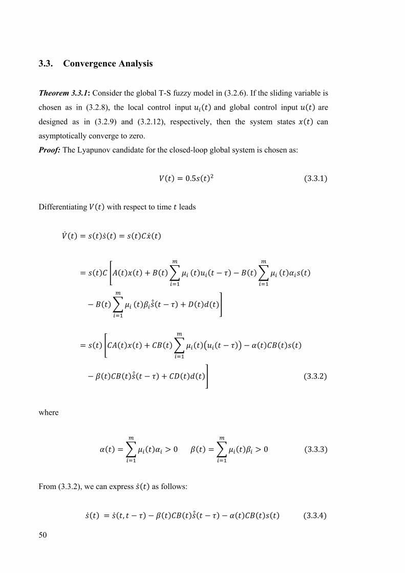
50

3.3. Convergence Analysis

Theorem 3.3.1: Consider the global T-S fuzzy model in (3.2.6). If the sliding variable is

chosen as in (3.2.8), the local control input and global control input are

designed as in (3.2.9) and (3.2.12), respectively, then the system states can


Proof: The Lyapunov candidate for the closed-loop global system is chosen as:

0.5 3.3.1

Differentiating with respect to time leads

3.3.2

where

0 0 3.3.3

From (3.3.2), we can express as follows:

, 3.3.4

51

where

, 3.3.5

Adding the term to (3.3.4), we have

,

| , |

3.3.6

Remark 3.3.1: Considering the continuity of both and , , we see that, as

the time delay is sufficiently small, we can always find a constant M >>1 such that the

following inequality is held:

| , |1

3.3.7

for , 0, 0 and 0.

Using (3.3.7) in (3.3.6), we obtain

1

3.3.8

Further, the approximation error between and is defined as:

3.3.9

For 0and 0,there exists a positive number , such that the


52

3.3.10

with 0 ≪ 1.

Then, using (3.3.9) and (3.3.10) in (3.3.8) leads

1

3.3.11

For the case that s :

If 0,

1

3.3.12

If the control parameter is chosen to satisfy the following condition:

11 1

3.3.13

then

1

3.3.14

(3.3.14) shows that the sliding mode-like learning controller in (3.2.12) always makes

the smaller than as 0.

Suppose that, at time , 0. Then, at the time , we can express

(3.3.4) as:

53

,

3.3.15

Considering the fact that

0 3.3.16

if the control parameter is chosen to satisfy the following condition:

, 3.3.17

then

,

0 3.3.18

(3.3.12)-(3.3.18) indicate that the sliding mode-like learning controller in (3.2.13) is

capable of driving the closed-loop system dynamics to move from the unstable domain

to the stable domain, and thus, ensure that

0

If 0, (3.3.11) can be expressed as:

1

1

11

54

0 3.3.19

Thus,

0

For the case that s :

If 0, we can express (3.3.6) as:

| , |

1

11

| | 3.3.20

Thus,

0

If 0,

| , |

1

1

| |

3.3.21

55

Suppose that, at time , 0

At the time , we can express (3.3.4) as:

,

3.3.22

Considering the fact that

0 3.3.23

we can also choose a proper in the sense that the inequality in (3.3.17) is

satisfied. Therefore,

,

0 3.3.24

(3.3.21) to (3.3.24) means that

0

In summary, we can conclude that the global controller in (3.2.12) can ensure

0 3.3.25

Both the sliding variable and the state variable vector can then asymptotically

converge to zero.

Remark 3.3.2: The inequality in (3.3.7) is called the Lipschitz-like condition [133] that

is simply another version of the continuity of the derivative of the Lyapunov function

in the state space. However, the embedded advantage of using the Lipschitz-like

condition is that no information on the upper and the lower bounds of uncertain

parameters is required for the design of the learning control in (3.2.12). Thus, the

56

control system design has been greatly simplified, compared with the conventional

SMC design in [14], [16], [17], [117], [118], and [130-132],

Remark 3.3.3: It is seen from Theorem 1 and the related mathematical discussions in

this section that the sliding mode-like learning control in (3.2.12) is capable of

continuously adjusting the direction of the convergence of the sliding variable, based on

the recent stability history of the closed-loop system, and driving the closed-loop system

to move towards to the sliding surface. Although the sliding variable may not reach the

sliding surface in a finite time, it can asymptotically converge to the sliding surface, and

the system states can also asymptotically converge to zero.

Remark 3.3.4: The claims in (3.3.16) and (3.3.23) are valid. Recall that, at time

,

0 3.3.26

3.3.27

and

sign( )=sign( ) 3.3.28

The control parameter can then be defined as:

0 3.3.29

Thus, the following inequality is held:

0 3.3.30

and together with the discussions in (3.3.15)-(3.3.18) and (3.3.22)-(3.3.24), we ensure

57

0 3.3.31

Remark 3.3.5: The robustness of the proposed scheme is another important feature. It is

seen from (3.2.12) that no information on the system parameters and model structure is

required for controller design, although the complex system may have uncertainties.

The sliding mode-like learning control signal in (3.2.12) is simply computed based on

the estimation of the most recent stability status of the closed-loop system and the

current measurements of the state variables.

3.4. An illustrative Example

Consider the following inverted pendulum on a cart with its dynamics as follows [15],

[17]:

22

43

3.4.1

where is the angle of the pendulum from the vertical, is the angular velocity,

9.81m/sis the gravity constant, is the mass of the pendulum rod, is the mass

of the cart, 2 is the length of the pendulum, is the control force applied to the cart,

parameter 1/ and the initial values of the state variables are

/10and 0, respectively.

In this simulation, the system parameters are as follows:

2.0kg, 8.0kg, 2 1.0m

with the T-S modelling technique described in Section 3.2, we represent the system in

(3.4.1) in state space as follows:

∶ IF isabout0, isabout0

58

THEN

∶ IF isabout0, isabout 4

THEN

∶ IF isabout /3, isabout0

THEN

∶ IF isabout /3, isabout 4

or isabout /3, isabout 4

THEN



THEN

3.4.2

where

0 117.2941 0

00.1765

0 114.4706 0

00.1765

0 15.8512 0

00.0779

0 17.2437 0.5399

00.0779

0 17.2437 0.5399

00.0779

3.4.3

59

The fuzzy membership functions for state variables and are chosen as in

Figures 3.1(a) and 3.1(b), respectively.

Figure 3.1(a) The membership functions of state

Figure 3.1(b) The membership functions of state

Based on (3.2.9)-(3.2.12), we have designed the global sliding mode-like learning

controller as follows:

-8 -6 -4 -2 0 2 4 6 80

0.1

0.2

0.3

0.4

0.5

0.6

0.7

0.8

0.9

1

x1

Mem

bers

hip

Func

tion

M1M2

-4 -3 -2 -1 0 1 2 3 40

0.1

0.2

0.3

0.4

0.5

0.6

0.7

0.8

0.9

1

x2

Mem

bers

hip

Func

tion

M1M2

60

3.4.4

Figures 3.2(a), 3.2(b) and 3.2(c) show the sliding variable , system state as

well as its derivative , and the global control input , respectively, where the

sliding mode parameter matrix is chosen as 5 1 ,the sampling period is∆

0.005 , the time delay ∆ , and the control parameters in (3.4.4) are set to

⋯ 20 & ⋯ 1.

It is seen that the sliding variable converges to zero in 2 seconds, the system states

and then exponentially converges to zero. In addition, the global control

signal is completely chattering-free.

Figure 3.2(a) Sliding variable (Sliding mode-like learning control)

0 1 2 3 4 5 6 7 8 9 10-0.2

0

0.2

0.4

0.6

0.8

1

1.2

1.4

1.6

Time t (sec)

The

slid

ing

mod

e va

riabl

e s(

t)

61

Figure 3.2(b) States and responses (Sliding mode-like learning control)

Figure 3.2(c) The control input (Sliding mode-like learning control)

For comparison purpose, Figures 3.3(a), 3.3(b) and 3.3(c) show the simulation results of

the closed-loop system with the conventional SMC [118], where the initial values of the

state variables and the sampling period are the same as the ones in Figures 3.2(a), 3.2(b)

and 3.2(c). It has been seen that, although the convergence speeds of both the proposed

learning control and the conventional SMC are nearly the same, the learning control

signal in Figure 3.2(c) is smooth and chattering-free. Such an excellent property makes

the proposed learning control more practical than the conventional one.

0 1 2 3 4 5 6 7 8 9 10-1.4

-1.2

-1

-0.8

-0.6

-0.4

-0.2

0

0.2

0.4

Time t (sec)

The

syst

em s

tate

s x1

(rad)

and

x2(

rad/

s)

x1x2

0 1 2 3 4 5 6 7 8 9 10-40

-20

0

20

40

60

80

100

120

140

160

Time t (sec)

The

cont

rol i

nput

sig

nal (

N)

62

Figure 3.3(a) Sliding variable (Conventional SMC)

Figure 3.3(b) States and responses (Conventional SMC)

0 1 2 3 4 5 6 7 8 9 10-0.2

0

0.2

0.4

0.6

0.8

1

1.2

1.4

1.6

Time t (sec)

The

slid

ing

mod

e va

riabl

e s(

t)

0 1 2 3 4 5 6 7 8 9 10-1.4

-1.2

-1

-0.8

-0.6

-0.4

-0.2

0

0.2

0.4

Time t (sec)

The

syst

em s

tate

s x1

(rad)

and

x2(

rad/

s)

x1x2

63

Figure 3.3(c) The control input (Conventional SMC)

3.5. Conclusion

In this chapter, a sliding mode-like learning control for a class of SISO complex

systems with the T-S fuzzy models has been developed. It has been shown that the

Lipschitz-like condition has been used to replace the upper and the lower bounds’

information for the controller design. Such a revolutionary idea has made the controller

design much easier than the one of the conventional sliding mode controllers. In

addition, the learning technique, proposed in this research, is another light point in the

sense that it can make the closed-loop system move from the unstable domain to the

stable domain, and thus, guarantees the stability of the closed-loop system. The futher

work is to combine the sliding mode-like learning control teachnique with the dominant

control principle in [16], [17], [118] to enchance the function of the sliding mode-like

learning control with various types of applications and it’s robust control.

0 1 2 3 4 5 6 7 8 9 10-200

-150

-100

-50

0

50

100

150

Time t (sec)

The

cont

rol i

nput

sig

nal (

N)

65

Chapter 4

Sliding Mode Learning Control of Fuzzy

Uncertain Continuous-time SISO Systems

In this chapter, a sliding mode learning control scheme is developed for a class of

continuous-time SISO complex systems. It is seen that a global T-S fuzzy model is first

built up to describe the complex system dynamics in the state-space, and a local sliding

mode learning controller is designed based on each local linear model. The concept of

dominant control principle can then be used to determine the global control signal to

ensure that the closed-loop system is globally asymptotically stable. As a learning

control, the control signal is updated by a correction term designed with the information

of the most recent stability history of the closed-loop system, and such a learning

strategy can always ensure that the asymptotic convergence of the closed-loop system is

achieved. The major advantage of the proposed control scheme is that the information

about the system uncertainties is no longer required for the controller design. A

simulation example is presented to demonstrate the effectiveness of the proposed SMC

control through comparison with the conventional SMC and H-infinity control.

4.1. Introduction

The fuzzy modelling technique offers an effective method to model the practical

systems that are highly complex and nonlinear [14], [128], [145-147]. Although a neural

network based modelling technique can also perform well in many cases, the fuzzy

modelling technique is capable of utilizing both the qualitative and quantitative

information about a complex system to construct its mathematical model with the help

of IF-THEN rules. The T-S fuzzy modelling technique is commonly used to develop a

systematic approach to approximate a class of complex systems by generating fuzzy

66

rules from a given input-output data set [4], [128], [129], [148]. The performance of this

technique depends on the number of fuzzy rules, the types of membership functions, the

consequent regressors and the measurable system variables. A great number of

theoretical results on system approximation have shown that, the T-S fuzzy modelling

technique can approximate any complex system to any desired degree of accuracy[4],

[9] ,[14-17], [117], [118], [128], [129], [148], [149].

Over the past two decades, the development of control schemes for better

robustness, performance and efficiency of T-S model-based fuzzy control systems has

attracted a lot of attention from researchers. There are plenty of control schemes related

to this research topic e.g. H-infinity control, SMC and guaranteed cost control [11], [14-

19], [117], [128], [137], [150-152]. The key technical problems such as conservative

stability condition, chattering and requiring information about the uncertain system

dynamics associated with the controller designs remain challenging research questions

in control engineering. In [15], the H-infinity control scheme is developed based on

norm bounded uncertainties. However, the drawback of this approach is that

information about system uncertainties needs to be known in the controller design. In

[16], [117], [132] and [157], the conventional SMC have been used to stabilize T-S

model-based fuzzy control systems and improve the robustness with respect to system

uncertainties and disturbances.

Nevertheless, the undesired chattering in the control signal is the main obstacle

for practical sliding mode controller implementation [2]. The chattering phenomena

may excite unmodeled high frequency dynamics, which degrades the performance of

the system and may lead to instability. Moreover, it results in low control accuracy, high

heat losses in electric power circuits and high wear of moving mechanical parts. The

boundary layer control technique is the common approach for eliminating the chattering

by replacing the sign function in the sliding mode controller designs with a saturation

function. However, the robustness of SMC is also compromised. Hence, the quest for

developing a new control technique for eliminating chattering while preserving the

robustness of the sliding mode appears to be a major challenge in the development of

SMC.

67

The traditional control structure for a T-S model based fuzzy control system is

PDC in which the global fuzzy control law can be obtained by aggregating all the local

controllers using a fuzzy inference law [4], [153]. In [4], [11] and [148], a fuzzy

feedback control law is designed based on some stability criteria. However, the stability

conditions require that for all the local linear models a common positive-definite matrix

P must be found [154], [155]. Finding the common positive matrix from a Riccati

equation might lead to a feasibility problem in which there is no solution for an LMI

expression and the process of finding the solution is complex.

In [156], a sliding mode-like learning control scheme is developed to drive the

sliding variable move towards to the sliding surface. Although the sliding variable may

not reach the sliding surface in a finite time, it can asymptotically converge to the

sliding surface, and the system states can then asymptotically converge to zero. Similar

to the fuzzy PDC control structure, the aggregated control parameters are required to

satisfy the design criteria based on some stability conditions. Therefore, this constraint

has greatly limited applications of the learning control scheme for the T-S model based

fuzzy system. It is hard to stabilize the global fuzzy system by means of amalgamating

the control signal from each subspace using a fuzzy inference law.

In this chapter, the global control signal is determined by the control signal of

the dominant linear model which dominates the entire dynamics of the global fuzzy

system as in [16], [17], [118]. In order to design an effective controller for better

performance, efficiency and robustness, a sliding mode learning control scheme has

been developed. The control signal is updated by a correction term designed with the

information of the most recent stability history of the closed-loop system. The effect of

the system uncertainties on the closed-loop system has been completely eliminated by

designing the sliding mode learning controller based on the Lipschitz-like condition

proposed in [133]. It is worth noting that the uncertain system dynamics can be

embedded into the Lipschitz-like condition as shown in [133], [135], [139-141], [156].

The controller designs with the aid of the Lipschitz-like condition can ensure the closed-

loop system behaves with a strong robustness with respect to unknown uncertainties and

disturbances. The major advantage of the proposed control scheme is that the

information about the system uncertainties is no longer required in the controller design.

68

Meanwhile, the chattering phenomenon that frequently appears in conventional SMC

systems is also eliminated without deteriorating the robustness of the system

The remainder of the chapter is organised as follows: In Section 4.2, the T-S

fuzzy modelling of a class of continuous-time SISO complex systems is formulated. In

Section 4.3, the sliding mode learning control scheme is proposed. In Section 4.4, the

convergence analysis of the closed-loop system with the proposed control scheme is

discussed in detail. In Section 4.5, simulation results are provided to show the

effectiveness of the proposed control scheme. Section 4.6 provides conclusions and

some further work.


Consider the following T-S fuzzy models to represent a class of complex SISO systems

with both fuzzy inference rules and local uncertain linear dynamic models [15]-[17],

[117], [118]:

∶ IF is AND… is

THEN

∆ ∆ 4.2.1

for 1,2, … ,


1,2,… , the fuzzy sets, the number of fuzzy sets, ≔ , ,… ,

contains some measurable system variables, and are and 1parameter

matrices, ∈ the system state vector, ∈ is the control input, ∆ and

∆ are and 1unknown system uncertainties, respectively.

Denoting as the normalized fuzzy membership function:

∑

4.2.2

69

where

4.2.3

0 4.2.4

and

1 4.2.5

Using the T-S fuzzy inferences [16], [117], [132], we obtain the global fuzzy model of

the complex systems as follows:

4.2.6

where

4.2.7

∆ ∆ 4.2.8

Definition 4.2.1: The fuzzy set is a binary set ,

where is the point at 1 and is called the crisp point of

[157].

Definition 4.2.2: If the controllability matrix , , … , , for

1,2, … , has a full rank of n, the local subsystems in (4.2.1) are locally controllable.

Definition 4.2.3: If the controllability matrix , , , … , has a full

rank of n. The global fuzzy model in (4.2.6) is globally controllable in the state space.

70

To proceed, we will assume that the (4.2.1) and (4.2.6) are both locally and globally

controllable. By using the sliding mode learning control technique [133], [156] and

dominant control principle [16], [17], [118], a global sliding mode learning controller

can be designed such that the closed-loop system is asymptotically stable.

4.3. Sliding Mode Learning Control

In this chapter, a sliding variable is defined as:

4.3.1

where ∈ is the sliding parameter matrix, which is selected to make the dynamics

of 0 Hurwitz.

For the fuzzy system described in (4.2.1)-(4.2.8), we propose the following local sliding

mode learning controller for the subsystem:

∶ IF is AND… is

THEN

∆ 4.3.2

for 1,2, … , .


∆ for 0

0for 0 4.3.3

where 0 , 0 and 0 in (4.3.3) are the control parameters to be

determined later, is the estimate of , is the time delay. The

minimum value of is actually equal to the sampling period in practice.

71

The estimation of can be achieved by using a numerical differentiator as

follows:

4.3.4

Remark 4.3.1: The terms and in (4.3.3) behave like inertia terms,

and by properly choosing the value of and , the asymptotic convergence of the

closed-loop system can be achieved. In addition, the correction term is used

to check the most recent stability status of the closed-loop system and update the control

signal. If the most recent information shows that the system is unstable, the term

is capable of adjusting the control signal in the sense that the closed-loop

system can be driven from the unstable domain to the stable domain. The merits of these

points can be seen from the convergence analysis in the next section.

Remark 4.3.2: It is important to note that the local linear models in (4.2.1) represent the

local dynamics of a class of continuous-time SISO complex systems in the subspaces of

the state space which are smoothly connected by fuzzy membership functions. However,

although each linear model with its local sliding mode controller in each subspace is

asymptotically stable, global asymptotic stability may not be guaranteed in the

overlapping regions of fuzzy sets where several subsystems are activated at the same

time to certain degrees [17].

Considering the fact that the local linear model in (4.2.1) with the maximum

membership function dominates the entire system dynamics, we can design the global

control [17], [157]. Firstly, the global control is inferred as:

4.3.5

Secondly, according to the dominant control principle [16], [17], [118], we can

use , the local control signal for the kth subsystem model with the maximum

membership function, to replace in (4.3.5). The global control can be expressed as

72

∆ 4.3.6

∆

where

: max , …, 4.3.7

Remark 4.3.3: It is seen that, no sign function of the sliding variable is involved in

the control signals and hence both the local control inputs and the global control input

enjoy chattering-free characteristics.

Remark 4.3.4: As shown in [16], [17], [118], the proposition of the dominant control

principle can greatly simplify the T-S model based fuzzy control system designs for

complex systems. Compared with the PDC approach [4], [153], the dominant control

approach can avoid the problem of finding a common positive solution to satisfy the

design criteria based on some stability conditions. The merits of the proposed control

with the aid of a dominant control principle can be seen from a section of the

convergence analysis and simulation results.


Theorem 4.4.1: Consider the global fuzzy system in (4.2.6). If the sliding variable is

chosen as in (4.3.1), the local control input and global control input are

designed as in (4.3.2) and (4.3.6), respectively, then the system trajectory can


Proof: The candidate of Lyapunov function for the global closed-loop system is chosen

as:

0.5 4.4.1

Differentiating with respect to time leads to

73

∆ ∆

,

4.4.2

where

, 4.4.3


,

74

,

4.4.4

where

4.4.5

Remark 4.4.1: Considering the continuity of both and , , with the

time-delay chosen to be sufficiently small, we may always find a constant M >>1 such

that the following inequality is held [133], [156]:

, 1

4.4.6

for , 0, 0 and 0.

It is important to note that the inequality (4.4.6) is called the Lipschitz-like condition

[133], [156]. The , is the derivative of the present Lyapunov function with the

recent control input, is the derivative of the most recent Lyapunov function.

The Lipschitz-like condition which describes the difference between these two

derivatives is very small as the sampling time is sufficiently small. The uncertain system

dynamics are all embedded into the left-hand side of (4.4.6). Therefore, the information

on the upper and the lower bounds of the system uncertainties is no longer required in

the controller design with the aid of the Lipschitz-like condition. In addition, the

Lipschitz-like condition provides a learning control strategy for us to design the

controller. The control signal is recursively updated based on the most recent stability

history of the closed-loop system. The merits of this control structure can be seen from

the following stability analysis.


75

1

4.4.7

where

4.4.8

Remark 4.4.2: As the time delay is sufficiently small, can be reasonably

assumed to have the same sign as , that is,

4.4.9

for 0and 0.

The approximation error between and is defined as:

4.4.10

For 0and 0,there exists a positive number , such that the


4.4.11

with 0 ≪ 1,

then using (4.4.10) and (4.4.11) in (4.4.7) leads to

1

76

4.4.12

If 0


1

1

4.4.13

Remark 4.4.3: It is important to note that the sliding mode parameter for each

linearized subsystem is designed to ensure the closed-loop system is globally

asymptotically stable, and also it satisfies the following conditions:

1 0 4.4.14

11

1

4.4.15

From (4.4.15), we can determine the control parameter . Then, using (4.4.15) in

(4.4.13) leads to

1

1

4.4.16

77

The inequality (4.4.16) shows that the global sliding mode learning controller in (4.3.6)

always makes the smaller than as 0.

Suppose that, at time , 0

, 4.4.17

From (4.4.17), we can express the terms as

, 0 4.4.18

For 0, (4.4.18) means that

0 4.4.19

It is seen from (4.4.18) that, the term , neutralises the negative force from

the global sliding mode learning controller in (4.3.6). However, the inequality in (4.4.19)

shows that the controller still continuously tries to drive the system energy towards the

direction of 0 . Moreover, the controller is designed to have inertial terms

and to force the 0.

At the time , we can express (4.4.17) as:

,

,

4.4.20

if the control parameters and are chosen to satisfy the following condition

78

, 4.4.21

then using (4.4.21) in (4.4.20),

, –

0 4.4.22

If 0

Using (4.4.15) in (4.4.12) leads to

11

11

0 4.4.23

(4.4.13)-(4.4.23) indicate that the global sliding mode learning controller in (4.3.6) is

capable of driving the closed-loop system dynamics to move from the unstable domain

to the stable domain, and thus, ensures that 0 . The sliding mode learning

control law in (4.3.6) ensures that both the sliding variable and the system states

asymptotically converge to zero. The merits of both the asymptotic convergence of the

closed-loop system and the chattering-free characteristics of the proposed sliding mode

learning controller can be further verified from the simulation results in the next section.

Remark 4.4.4: As the sliding variable asymptotically converges to zero, the

relationship between and as time → ∞ is definite as:

lim→ 4.4.24

where 0 | | 1,

79

then the correction term ∆ in the sliding mode learning controller in (4.3.2)

satisfies:

lim→

∆ lim→

lim→ 2

lim→ 2 2

11

0 4.4.25

Therefore, there is no singularity in the control signal . This point will be clearly

seen from a section of the simulation results.

Remark 4.4.5: The design of sliding surface is a major problem in this chapter. The pole

placement approach [158] and the hyperplace design approach [159] are commonly

used to design sliding parameter of sliding surface . All the methods can be used

for the design of for the fuzzy control system. However, the design of needs to

satisfy the design criteria specified in Remark 4.4.3

Remark 4.4.6: It is well known that, in conventional SMC, the upper and lower bounds

of system uncertainties are often required for designing a sliding mode controller.

However, as seen in both the local sliding mode learning control in (4.3.2) and the

global fuzzy control law in (4.3.6) in this chapter, no information about unknown

system parameter is needed for the design of both the local sliding mode and the global

sliding mode controller. Therefore, the proposed control scheme is robust and is the

most suitable for control of large-scale systems with large uncertain dynamics and

unknown dynamic interactions.

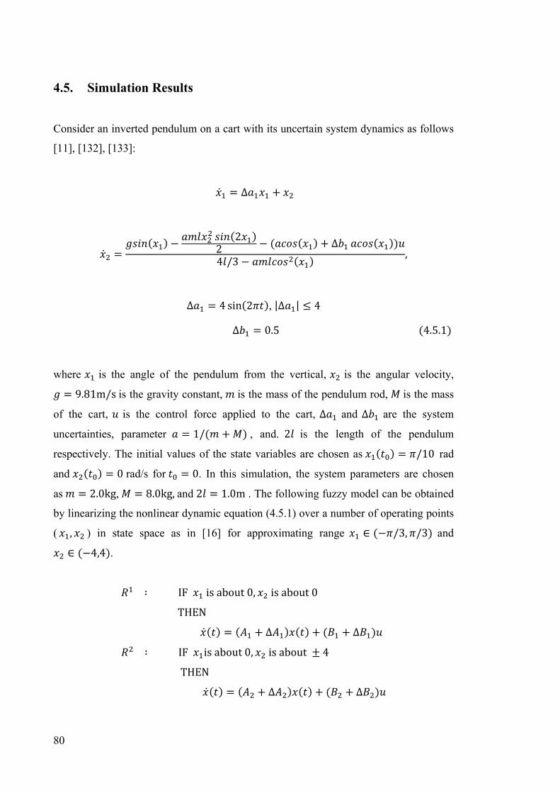
80

4.5. Simulation Results

Consider an inverted pendulum on a cart with its uncertain system dynamics as follows

[11], [132], [133]:

∆

22 ∆

4 /3,

∆ 4 sin 2 , |∆ | 4

∆ 0.5 4.5.1

where is the angle of the pendulum from the vertical, is the angular velocity,

9.81m/sis the gravity constant, is the mass of the pendulum rod, is the mass

of the cart, is the control force applied to the cart, ∆ and ∆ are the system

uncertainties, parameter 1/ , and. 2 is the length of the pendulum

respectively. The initial values of the state variables are chosen as /10rad

and 0 rad/s for 0. In this simulation, the system parameters are chosen

as 2.0kg, 8.0kg,and 2 1.0m . The following fuzzy model can be obtained

by linearizing the nonlinear dynamic equation (4.5.1) over a number of operating points

( , ) in state space as in [16] for approximating range ∈ /3, /3 and

∈ 4,4 .

∶ IF isabout0, isabout0

THEN

∆ ∆

∶ IF isabout0, isabout 4

THEN

∆ ∆

81

∶ IF isabout /3, isabout0

THEN

∆ ∆



THEN

∆ ∆



THEN

∆ ∆ 4.5.2

where

0 117.2941 0

00.1765

0 114.4706 0

00.1765

0 15.8512 0

00.0779

0 17.2437 0.5399

00.0779

0 17.2437 0.5399

00.0779

∆ ∆ …∆ ∆ 00 0

∆ 0.5 ∆ 0.5 ∆ 0.5

∆ 0.5 ∆ 0.5 4.5.3

we use the following fuzzy membership functions for state variables and :

/1

1 / 1

1 /

/1

1 / 1

1 /

1 / / 1 4.5.4

82

These membership functions are shown in Figure 4.1.

Figure 4.1 The membership functions of fuzzy sets and

The membership functions for 1st-5th rules of the fuzzy model are selected based on the

extension principle.

: ∗

: max ∗ , ∗

: max / ∗ , / ∗

: max / ∗ , / ∗

: 1 4.5.5

Based on (4.3.2)-(4.3.7), we select the control signal of the dominant subsystem as the

global sliding mode learning controller:

∆ 4.5.6


-3 -2 -1 0 1 2 30

0.5

1

Membership Function of fuzzy set x1(rad)

M(x

1)

MApi/3MA-pi/3MA0

-3 -2 -1 0 1 2 30

0.5

1

Membership Function of fuzzy set x2 (rad/s)

M(x

2)

MB4MB-4MB0

83

∆ for 0

0for 0 4.5.7

where

: max ,…,

The sliding mode parameter matrix is chosen as 5 1 , the sampling period

is∆ 0.001 , the time delay ∆ .

It is easy to check that

0.4414 0 4.5.8

is satisfied for all and . Also, in this simulation, we assume =20 and 0.001

1

0.051 4.5.9

The control parameter is designed to satisfy the following condition:

0.1907 0.4414 0.051 4.5.10

Therefore, the control parameters in (4.5.7) are set to 6, 0.2 and 0.4.

Figures 4.2(a) and 4.2(b) show the sliding variable , the global control input

and system states and . It is clearly seen that in Figures 4.2(a) and 4.2(b) the

sliding variable converges to zero in 0.5 seconds, the states and can then

asymptotically converge to zero. The concept of the Lipschitz-like condition is verified

in Figure 4.2(c), the inequality in (4.4.6) is always satisfied. In addition, the control

signal is completely chattering-free.

84

Figure 4.2(a) Sliding variable and control input

(Sliding mode learning control)

Figure 4.2(b) States and responses (Sliding mode learning control)

0 0.5 1 1.5 2 2.5 3 3.5 4 4.5 5-1

0

1

2

Time t (sec) sampling period:0.001s

The

slid

ing

mod

e va

riabl

e s(

t)

0 0.5 1 1.5 2 2.5 3 3.5 4 4.5 5-50

0

50

100


The

cont

rol i

nput

sig

nal(N

)

0 0.5 1 1.5 2 2.5 3 3.5 4 4.5 50

0.1

0.2

0.3

0.4


The

syst

em s

tate

s x1

(rad)

0 0.5 1 1.5 2 2.5 3 3.5 4 4.5 5-1.5

-1

-0.5

0

0.5


The

syst

em s

tate

s x2

(rad/

s)

85

Figure 4.2(c) Validation of the Lipschitz-like condition (Sliding mode learning control)

For comparison purposes, the conventional sliding mode and H-infinity controller are

developed based on T-S fuzzy models in (4.5.2). Firstly, Figures 4.3(a) and 4.3(b) show

the simulation results of the closed-loop system using the conventional SMC [118],

where the control gains … 15, the initial values of the state variables and

the sampling period are the same as the previous ones. It has been seen that, although

the convergence speeds of the proposed sliding mode learning control and the

conventional SMC are nearly the same, the sliding mode learning control signal in

Figure 4.2(a) is smooth and chattering-free. Such an excellent property obviously makes

the proposed sliding mode learning control more practical.

0 0.5 1 1.5 2 2.5 3 3.5 4 4.5 50

0.05

0.1

0.15

0.2

0.25


Lips

chitz

-like

con

ditio

n (4

.4.6

)

Left hand side of (4.4.6)Right hand side of (4.4.6)

86

Figure 4.3(a) Sliding variable and control input (Conventional SMC)

Figure 4.3(b) States and responses (Conventional SMC)

Next, the H-infinity control scheme is used to compare the control performance of

different controllers. The following control gains can be determined by the H-infinity

attenuation technique in [132]:

222.4850.38 , 188.2546.34

0 0.5 1 1.5 2 2.5 3 3.5 4 4.5 5-1

0

1

2


The

slid

ing

mod

e va

riabl

e s(

t)

0 0.5 1 1.5 2 2.5 3 3.5 4 4.5 5-200

-100

0

100

200


The

cont

rol i

nput

sig

nal(N

)

0 0.5 1 1.5 2 2.5 3 3.5 4 4.5 50

0.1

0.2

0.3

0.4


The

syst

em s

tate

s x1

(rad)

0 0.5 1 1.5 2 2.5 3 3.5 4 4.5 5-2

-1.5

-1

-0.5

0


The

syst

em s

tate

s x2

(rad/

s)

87

211.6578.21 , 228.1085.38

235.9472.35 4.5.11

Figure 4.4(a) The control input (H-infinity control)

Figure 4.4(b) States and responses (H-infinity control)

The control performance of the H-infinity in Figures 4.4(a) and 4.4(b) are not as good as

the proposed sliding mode learning control method. The settling time is much longer

than conventional SMC and proposed sliding mode controller.

For a further comparison, we amplify the system uncertainty ∆ as follows:

0 0.5 1 1.5 2 2.5 3 3.5 4 4.5 5-10

0

10

20

30

40

50

60

70


The

cont

rol i

nput

sig

nal(N

)

0 0.5 1 1.5 2 2.5 3 3.5 4 4.5 5-0.2

0

0.2

0.4

0.6


The

syst

em s

tate

s x1

(rad)

0 0.5 1 1.5 2 2.5 3 3.5 4 4.5 5-1.5

-1

-0.5

0

0.5


The

syst

em s

tate

s x2

(rad/

s)

88

∆ 10 sin 2 4.5.12

Based on the uncertainty in (4.5.12), we redesign the control gains for the H-infinity

controller

1143.2258.9 , 967.3238.1

1279.6477.1 , 1329.6497.7

1375.3421.7 4.5.13

The attenuation performance of the H-infinity control with the control gains as set in

(4.5.13) are shown in Figures 4.5(a) and 4.5(b). In order to maintain the control

performance, a set of large gains are required for H-infinity control to compensate for

the effects of the uncertainties. However, large control gains will generate a large

overshoot in the control signal which is not suitable in real-time implementation.

Fig. 4.5(a): The control input (H-infinity control)

0 0.5 1 1.5 2 2.5 3 3.5 4 4.5 5-300

-200

-100

0

100

200

300

400

500


The

cont

rol i

nput

sig

nal(N

)

89

Figure 4.5(b) States and responses (H-infinity control)

The simulation results of the proposed sliding mode learning controller are shown in

Figures 4.6(a) and 4.6(b). The sliding mode parameter matrix is set as 15 1 , the

control parameters of the proposed controller remain the same as the previous ones. The

overshoot of the proposed control input signal in Figure 4.6(a) is much smaller than the

H-infinity control method in Figure 4.5(a). Meanwhile the proposed sliding mode

learning controller can ensure that the closed-loop system is globally asymptotically

stable without the need of adjusting the control gains , and .

Figure 4.6(a) Sliding variable and control input

0 0.5 1 1.5 2 2.5 3 3.5 4 4.5 50

0.5

1

1.5

2

Time t (sec) sampling period:0.001sTh

e sy

stem

sta

tes

x1(ra

d)

0 0.5 1 1.5 2 2.5 3 3.5 4 4.5 5-6

-4

-2

0


The

syst

em s

tate

s x2

(rad/

s)

0 0.5 1 1.5 2 2.5 3 3.5 4 4.5 50

2

4

6


The

slid

ing

mod

e va

riabl

e s(

t)

0 0.5 1 1.5 2 2.5 3 3.5 4 4.5 5-100

0

100

200


The

cont

rol i

nput

sig

nal(N

)

90

(Sliding mode learning control)

Figure 4.6(b) States and responses (Sliding mode learning control)

The merit of using the sliding mode learning control technique is that the controller can

guarantee the system states smoothly converge to zero. The system uncertainties have

been embedded in the Lipchitz-like condition as in (4.4.6). Hence, without relying on

the upper and the lower bounds of system uncertainties, the controller tunes the current

stability status of the system as it moves towards the stable region. The proposed

learning control method is less conservative than the conventional SMC method and H-

infinity control method. Therefore, it can be used for more complex control systems.

4.6. Conclusion

In this chapter, the sliding mode learning control has been developed for fuzzy uncertain

continuous-time SISO systems. It has been seen that the proposed sliding mode learning

control is capable of driving both the sliding variable and systems states to converge to

zero asymptotically based on the most recent stability status of the closed-loop system.

The concept of dominant control principle is used to facilitate the sliding mode learning

control scheme and enchance the function of the controller in different types of control

applications. The design criteria for sliding parameter have been proposed to ensure

0 0.5 1 1.5 2 2.5 3 3.5 4 4.5 50

0.1

0.2

0.3

0.4


The

syst

em s

tate

s x1

(rad)

0 0.5 1 1.5 2 2.5 3 3.5 4 4.5 5-3

-2

-1

0

1


The

syst

em s

tate

s x2

(rad/

s)

91

the stability of the closed-loop system. It has been further shown in the simulation

section that the proposed sliding mode learning control achieves much better results in

terms of robustness and performance as compared to the conventional SMC and H-

infinity control. The further work to apply the sliding mode learning control with the

adaptive estimation of control parameters for the large-scale systems is placed under

investigation.

93

Chapter 5

Robust Sliding Mode Learning Model

Reference Tracking Control for a Class of

Large-Scale Systems with Adaptive

Estimation

This chapter studies the problem of a sliding mode learning model reference tracking

control for a class of large-scale systems. The considered large-scale system contains a

number of nonlinear interconnected subsystems. The interconnection between these

subsystems may be nonlinear and unknown. The local dynamics of subsystems is first

described by a local linear model in the state-space. It is seen that a global T-S fuzzy

model can then be achieved by smoothly connecting the local linear model in each

subspace of the state space together via membership functions. A set of local chattering-

free sliding mode learning controllers is designed to ensure the stability of its

corresponding local linear model. According to the principle that the dominant

subsystem governs the global fuzzy model dynamics, a global control signal can be

determined to override the effects of nonlinear interconnections such that good tracking

performance is achieved. The advantage of the control structure is that a prior

knowledge of the upper bounds of interconnection among subsystems is not required in

the proposed learning controller design. A simulation example is given to show the

excellent tracking performance and effectiveness of the proposed sliding mode learning

control scheme.

5.1. Introduction

In recent years, there has been rapidly growing interest in the control of a class of large-

scale systems. There are plenty of successful applications related to this research topic

such as multirobot systems, electric power systems, aerospace systems, process control

94

systems and transportation networks. A large-scale system consists of a number of

subsystems that serve particular functions and exchange information between the

subsystems in the sense that the subsystems have become increasingly large in

complexity in their structure. That is the main reason why control of complex

behaviours in large-scale systems has received a great deal of attention in recent studies

[160]-[164]. From a system theoretic point of view, a large-scale system can be treated

as a set of interconnected complex nonlinear systems.

In the past few years, many modelling methodologies have been developed to

model large-scale systems for investigating the stability property of the systems and

designing effective control strategies [165]-[170]. In [167], a large-scale system is

composed of linearized interconnected subsystems, and the authors have defined a

switching function for each subsystem. Jaint et al. considered a class of interconnected

systems which can be transformed to the decentralized strict feedback form in [168].

However, the major drawbacks of conventional modelling approaches are attributed to

(i) the lack of a systematic method for its stability analysis, (ii) various assumptions

required to model the interconnected subsystems, (iii) the linearization technique and

linear robust control are only applicable to some specific large-scale systems, (iv)

difficult to obtain the system dynamics in practice [165]. Recently, T-S fuzzy modelling

technique is used to develop a systematic approach to model the large-scale systems

[166], [171], [172]. It has the capability of approximate the systems to arbitrary degrees

of accuracy.

In order to provide a simple and robust control scheme for a class of large-scale

systems, the researchers have noted many possible control solutions of applying the T-S

fuzzy modelling technique. Wang et al. developed the decentralized PDC for large-scale

T-S Fuzzy systems [166]. Some sufficient conditions are based on Lyapunov criterion

and Riccati-inequality. In [171], a robust control problem is studied for a class of large-

scale networked control systems. Tseng et al. developed the -infinity decentralized

fuzzy control scheme to deal with the model reference tracking control problem [172].

The major defect of the decentralized PDC approaches is that the upper bounds of

nonlinear interconnections need to be known in controller designs. For large-scale T-S

Fuzzy systems, if the number of sub-models is large, finding the common positive

95

matrix by using LMI might cause a feasibility problem in which there is no solution for

LMI expression. In addition, the decentralized control scheme attempts to avoid

difficulties in complexity of design and storage requirements. However, there is still no

efficient way to cope with the decentralized control problem of large-scale nonlinear

interconnected systems i.e., to design a decentralized controller so that the states of the

system asymptotically track the given model reference inputs independent of any

nonlinear interconnections among the systems. As a result, many theoretical and

practical problems remain unsolved in this field.

The objective of this chapter is to address the problem of model reference

tracking control for a class of large-scale systems by applying sliding mode learning

control theory based on [133], [135], [139]-[141], [156]. Our interest in this problem is

motivated by the recent relative research works in [165]-[166] and [172] on T-S fuzzy

modelling and control of large-scale systems. In a large-scale system, global T-S fuzzy

models are first developed to model dynamics of nonlinear interconnected subsystems.

A set of local sliding mode learning controllers can then be designed to ensure the

stability of its corresponding local linear models which are smoothly connected by

fuzzy membership functions. For each subsystem, global fuzzy control can be

determined by the control signal of the dominant local linear model which dominates

the dynamics of the global T-S fuzzy model.

As a learning control, the control signal is updated by a correction term designed

with the information of the most recent stability history of the closed-loop system to

drive both the sliding variable and tracking error between system state and model

reference to asymptotically converge to zero. The prior information about the nonlinear

interconnections among subsystems is no longer required in the controller design with

the aid of the Lipschitz-like condition. The proposed sliding mode learning control in

this chapter is designed based on the concept of adaptive control laws in [17]. Unlike

the control strategy in [156], in which the sliding mode learning control parameters are

determined based on some stability criteria, in this chapter we use adaptive estimation

laws such that the control parameters are obtained as well for the proposed controller

design. The adaptive estimation laws are designed based on the most recent stability

96

status. It can be seen that, the estimation stops after the sliding variable reach the sliding

surface in which the behavior of the system depends on the design of the sliding surface.

The rest of this chapter is organised as follows: in Section 5.2, the T-S fuzzy

modelling of a class of large-scale systems and the sliding mode learning control with

adaptive estimation laws are formulated. In Section 5.3, the convergence analysis of the

closed-loop system with the proposed sliding mode learning control is discussed in

detail. In Section 5.4, a simulation example is given to illustrate the effectiveness of the

proposed control scheme. Section 5.5 provides the conclusions and some further works.


Suppose there is a large-scale system composed of nonlinear interconnected

subsystems. The dynamics of each subsystem can be represented by T-S fuzzy

models in subspaces of the state-space. The lth rule of the T-S fuzzy model for ith

subsystem is of the following form [166], [173]:

:

IF is AND… is

THEN,

5.2.1

for 1,2, … , ; 1,2, … ,

where the number of subsystems, the number of inference rules, 1,2, … , the fuzzy sets, the number of fuzzy sets, ∈ the state vector, ∈ the

input variable. ≔ , ,… , contains measurements of system variables,

represents the interconnection between subsystem and subsystem ,

and are and 1 parameter matrices, respectively.

Denoting as the normalized fuzzy membership function:

∑

5.2.2

97

where

5.2.3

0 5.2.4

and

1 5.2.5

and using the T-S fuzzy inferences [117], [156], [174],we obtain the global fuzzy model

of ith subsystem as follows:

5.2.6

where

,

5.2.7

For future consideration, we have the following assumptions [15],[133]:

Assumption 5.2.1: Each local subsystem in (5.2.1) is controllable, that is, the

controllability matrix

, , … , , for 1,2,… ,


98

Assumption 5.2.2: The global fuzzy model in (5.2.6) is controllable in the state space,

that is, the controllability matrix

, , , … ,


Consider a reference model for ith subsystem [117], [132], [166]:

5.2.8

where ∈ the reference state vector, ∈ the specific asymptotically

stable matrix and ∈ is the bounded reference input.

The tracking error is defined as:

… 5.2.9

where for 0,1, … , 1.

The error dynamics of ith closed-loop system can be obtained by using (5.2.6), (5.2.8)

and (5.2.9).

5.2.10

Remark 5.2.1: The objective of this chapter is to determine a control signal such

that the error dynamics of the ith closed-loop system asymptotically converges to zero.

It will be shown that prior knowledge of the upper bounds of the nonlinear

interconnections among subsystems is not required in the proposed controller design.

Such an advantage makes the proposed control scheme exhibit strong robustness against

unknown nonlinear interconnections.

99

For ith closed-loop system, a sliding variable is defined as:

5.2.11

where ∈ is the sliding mode parameter matrix, which is selected to make the

characteristic matrix of 0 Hurwitz.

In this chapter, the fuzzy sliding mode learning controller for its corresponse lth rule of

the T-S fuzzy model for ith subsystem is proposed as follows:

:IF is AND… is THEN ∆

5.2.12

for 1,2, … , , for 1,2, … ,


∆ for 0

0for 05.2.13

where 0 , 0 and 0 are control parameters, is the time delay,

is the first order derivative of 0.5 and is the estimate

of defined as:

5.2.14

Remark 5.2.2: One natural candidate of the control for the global fuzzy model in (5.2.6)

may be

5.2.15

100

The global control (5.2.15) requires the aggregated sliding mode learning control

parameters to satisfy the design criteria based on some stability conditions [156]. This

constraint has greatly limited applications of the learning control scheme for the control

of large-scale systems via T-S fuzzy models. Therefore, the concept of dominant control

principle is used to determine the global control signal and the robust control scheme

can then be developed to ensure that the ith closed-loop system is globally

asymptotically stable.

For ith closed-loop system, the global control is defined as:

∆ 5.2.16

where

: max , …, 5.2.17

Theorem 5.2.1: For the global fuzzy model of ith subsystem (5.2.6), if

1 0 5.2.18

and the control input (5.2.16) with the adaptation laws

5.2.19

5.2.20

5.2.21

then there exists amoment such that for , the system is asymptotically stable

[17].

101

Remark 5.2.3: It can be seen from the next section that the correction term ∆ is

continous all the time. Therefore, the local control inputs and global control input

in (5.2.12) and (5.2.16) are continuous as well. The merits of this point can be

seen in the stability analysis and simulation sections.


Theorem 5.3.1: Consider the global T-S fuzzy model in (5.2.5). If the sliding mode

variable is chosen as in (5.2.11), the local control input and global control input

are designed as in (5.2.16) with adaptation laws in (5.2.19), (5.2.20) and (5.2.21),

then the overall closed-loop system of the large-scale system, consisting of q subsystem

is asymptotically stable. Thus, the tracking error of each subsystem can asymptotically

converge to zero.

Proof: The Lyapunov candidate for the overall closed-loop system of the large-scale

system is chosen as:

0.5 0.5

0.5

0.5 5.3.1

for 1,2, …

where , and are adaptation errors.

The time derivative of is

102

5.3.2

Substituting (5.2.10) and (5.2.15) into (5.3.2) yields

5.3.3


∆

, ∆

,

103

,

5.3.4

where

,

5.3.5

and

5.3.6


,

,

5.3.7

where

5.3.8

Remark 5.3.1: Considering the continuity of both and , , with the

time-delay chosen to be sufficiently small, we may always find a constant >>1

such that the following Lipschitz-like condition inequality is held [156]:

104

,1

5.3.9

for , 0, 0 and 0.

The inequality (5.3.9) is called the Lipshitz-like condition [133]. It describes that the

difference between the present value of the gradient of the Lyapunov function and its

most recent value is very small as the time interval is sufficiently small. The uncertain

system dynamics are all embedded into left-hand side of (5.3.9). For the controller

designs with the aid of the Lipschitz-like condition, the knowledge of the upper bounds

of the interconnection between subsystem and subystem is no longer required. It

is expected that, in the control of large-scale systems with unknown dynamic

interactions, the Lipschitz-like condition will play a very essential role to relax

constraints on the robust controller design.


1

5.3.10

Remark 5.3.2: If the time delay is sufficiently small, it is reasonable to assume that

5.3.11

5.3.12

and

5.3.13

for 0, 0,and 0 ≪ 1

105

The inequality (5.3.13) implies that the approximation error between

and is very small as the time interval is sufficiently small.

Using (5.3.12) and (5.3.13) in (5.3.10) leads to

1

5.3.14

If 0

Substituting the condition (5.2.19), (5.2.20) and (5.2.21) into (5.3.10) yields

1

1

1

| |

5.3.15

The targeted is defined as

1

5.3.16

106

Then, using (5.3.16) in (5.3.15) leads to

1| |

5.3.17

The inequality (5.3.17) indicates that the global sliding mode learning controller in

(5.2.16) always makes the value of decrease when 0.

Remark 5.3.3: There exists a moment such that for , , and

. As long as the sliding surface is not reached, , and will increase by

, and until 0. Therefore, the requirement of a prior knowledge of

upper bounds of the , and is removed.

Suppose that, at the time and 0, we can express (5.3.4) as:

,

,

,

5.3.18

Consider the fact that

107

≅ 0 5.3.19

and

0 5.3.20

The targeted is defined as

,

5.3.21

then using (5.3.21) in (5.3.18),

≅ , 0 5.3.22

If 0


11

11

11

5.3.23

If the estimated control parameter is designed to satisfy the following condition:

108

11

10 5.3.24

Remark 5.3.4: It is worth noting that condition (5.3.24) highly depends on the design of

sliding parameter for each subsystem in the large-scale system. The design of

needs to ensure the closed-loop system is globally asymptotically stable, and also it

satisfies the condition specified in (5.3.24) and (5.2.18).

Using (5.3.24) in (5.3.23) leads to

11

0 5.3.25

Specifically, (5.3.25) means that

0 5.3.26

The proof indicates that the global sliding mode learning control in (5.2.16) is capable

of driving the ith closed-loop system dynamics to move from the unstable domain to the

stable domain. Thus, the overall closed-loop system of the large-scale system is

asymptotically stable and the sliding mode learning control law in (5.2.12) ensures that

both the sliding variable and tracking error also asymptotically converge to

zero.

109

Remark 5.3.5: As the sliding variable asymptotically converges to zero, the

relationship between and as time → ∞ is definite as:

→ 5.3.24

where 0 | | 1,

then the correction term ∆ in the sliding mode learning controller in (5.2.13)

satisfies:

→

∆→

→

| |2

2

→

1 1

2

1 1

2

→

1 1

2

1 1

2

0

110

Remark 5.3.5: It is important to note that, in conventional decentralized feedback

control approaches, the upper bound of interconnections is often required for designing

a feedback controller. In addition, solving the LMI matrix does not guarantee that the

positive definite is always available in practice, especially for large-scale systems.

However, in the proposed control scheme, no information about the unknown

interconnections is needed and no LMI matrix is required to be solved for the proposed

control scheme. Therefore, the proposed control scheme is suitable for large-scale

systems with unknown dynamic interactions.

The merits of both the asymptotic error convergence and the chattering-free

characteristics of the proposed sliding mode learning controller can be further verified

from the simulation example in the next section.

5.4. Simulation Results Consider a large-scale system S that is composed of three subsystems , and . The

rules of the T-S fuzzy model for each subsystem are shown as follows:

: ∶ IF isabout0, isabout0 THEN

,

∶ IF isabout0, isabout 1 THEN

,

∶ IF isabout 1, isabout0 THEN

,

: ∶ IF isabout0, isabout0

THEN

,

111


,

: ∶ IF isabout0, isabout0

THEN

,


,

(5.4.1) where

0 12 3

0 12.4 3.3

0 13 4

0 13 3

0 13.4 3.1

0 16 5.5

0 16.2 5.8

10 5.4.2

The fuzzy membership functions for state variables , , , ,

, are chosen as in Figures 5.1 (a), 5.1(b) and 5.1(c).

112

Figure 5.1(a) Membership functions of and

Figure 5.1(b) Membership functions of and

-3 -2 -1 0 1 2 30

0.1

0.2

0.3

0.4

0.5

0.6

0.7

0.8

0.9

1

Membership Function of x11 and x12

+10-1

-3 -2 -1 0 1 2 30

0.1

0.2

0.3

0.4

0.5

0.6

0.7

0.8

0.9

1


+10-1

113

Figure 5.1(c) Membership functions of and

The interconnections among the three systems are given as follows:

0.5. sin

0.5. sin

0.6. sin

0.6. sin

0.5. sin

0.5. sin 5.4.3

For tracking purpose, the each subsystem reference model is designed as follows:

0 110 10

010cos 0.5

0

10sin 0.5 5.4.4

Based on (5.2.12)-(5.2.17), we select the control signal of the local system model with

the maximum membership function as the global sliding mode tracking control for each

subsystem:

-3 -2 -1 0 1 2 30

0.1

0.2

0.3

0.4

0.5

0.6

0.7

0.8

0.9

1


+20-2

114

∆ (5.4.5)

for 1,2 and 3


∆ for 0

0for 05.4.6

and

: max , …, 5.4.7

The sliding mode parameter matrices are chosen as 10 1 , the

sampling period is∆ 0.001sec, the parameters , and in (5.2.19)-(5.2.21)

are set to be 20, 0.01 and 0.1 for 1,2 and 3 , the time delay

∆ and initial condition for each subsystem is 0 0.2; 0.5 , 0

0.2; 0.1 and 0 0.2; 0.1 .

It can be seen from (5.4.1) that

1 5.4.8

Also, in this simulation, we assume =50 and 0.001

1

0.021 5.4.9

The performance of the sliding mode learning controllers is shown in Figures 2(a), 2(b),

2(c) and 2(d).

Figures 2(a), 2(b), 2(c) and 2(d) show the state variables , ,

, and , , and global control

input , and , respectively. It is seen that, within 1 second, the tracking

115

error converges to zero. Also, the global sliding mode learning control signal is

continuous and chattering-free.

Figure 5.2(a) The states (t) and responses

Figure 5.2(b) The states (t) and responses

0 2 4 6 8 10 12 14 16 18 20-1

-0.5

0

0.5

1


The system state x11(rad)and reference state xr11(rad)

0 2 4 6 8 10 12 14 16 18 20-1

-0.5

0

0.5

1


The system state x12(rad/s)and reference state xr12(rad/s)

Reference Signal

Reference Signal

Tracking State

Tracking State

0 2 4 6 8 10 12 14 16 18 20-1

-0.5

0

0.5

1



0 2 4 6 8 10 12 14 16 18 20-0.5

0

0.5



Reference Signal

Reference Signal

Tracking State

Tracking State

116

Figure 5.2(c) The states (t) and responses

Figure 5.2(d) The global control input , and

It is clearly seen that in Figures 5.3, 5.4 and 5.5, the control parameters , and

accumulated until 0. Therefore, the asymptotical stability of the global fuzzy

system is guaranteed.

It is easy to check that

0.4895 0 5.4.9

is satisfy for all

0 2 4 6 8 10 12 14 16 18 20-1

-0.5

0

0.5

1



0 2 4 6 8 10 12 14 16 18 20-0.5

0

0.5

1



Tracking State

Tracking State

Reference Signal

Reference Signal

0 2 4 6 8 10 12 14 16 18 20-10

-5

0

5

10

15

20


The global fuzzy control input u1,u2 and u3

117

Figure 5.3(a) The adaptation parameters , and for

Figure 5.3(b) Sliding variable

0 0.5 1 1.5 2 2.5 30

0.5

1

1.5


The adaptation parameters for S1

alpha1kbeta1keta1k

0 0.5 1 1.5 2 2.5 3

-0.4

-0.2

0

0.2

0.4

0.6

0.8

1

1.2

1.4

1.6


The sliding variable for S1

118



0 0.5 1 1.5 2 2.5 30

0.5

1

1.5

2

2.5

3

3.5



alpha2kbeta2keta2k

0 0.5 1 1.5 2 2.5 3-2.5

-2

-1.5

-1

-0.5

0

0.5



119



5.5. Conclusion

This chapter has developed an adaptive sliding mode learning control scheme for the

trajectory tracking control of a class of large-scale systems with T-S fuzzy models. It

has been shown that the proposed controller is capable of efficiently adjusting the

closed-loop response based on the most recent history of the closed-loop stability and

ensuring a robust tracking performance. Meanwhile, the principle of the dominant

0 0.5 1 1.5 2 2.5 30

0.5

1

1.5

2

2.5



alpha3kbeta3keta3k

0 0.5 1 1.5 2 2.5 3-0.5

0

0.5

1

1.5

2



120

subsystem helps simplify the global controller design. The adaptive estimation laws

accumulate the nonzero distance to the sliding surface for the estimation of the control

parameters. The simulation results have demonstrated the excellent tracking

performance of the proposed scheme. The further work to extension the proposed

scheme to the control of MIMO nonlinear systems, sampled data systems, and the

design of the sliding mode learning control based observers are under the investigation.

121

Chapter 6

Conclusions

In this chapter, the major contributions of the current work are highlighted, and some of

the relevant future research directions are given.

6.1. Summary of Contributions

This thesis has developed a number of robust sliding mode learning control algorithms

for complex systems with dynamic fuzzy models. The focus of this thesis is on the

study and improvement of sliding mode learning control design, in order to achieve

strong robustness against parameter variations, external disturbances, and nonlinear

interconnections. Different from conventional SMC, the information about the unknown

system dynamics is not required for the design of the learning controller and the control

input is chattering-free. The key contributions of this thesis are summarized as follows:

Chapter 2 of this thesis has provided the fundamental fuzzy set theory for fuzzy logic

and fuzzy systems which are being applied in this thesis. The fuzzy sets, fuzzy set

operations, fuzzy relations and compositions, extension principle and fuzzy inference

systems have been outlined. The basic concepts of Mamdani fuzzy systems and T-S

fuzzy systems have been discussed. By comparing these two systems, the advantages of

T-S fuzzy systems against Mamdani fuzzy systems in the control area are highlighted.

Lyapunov stability theory is provided in order to analyse the stability properties of T-S

fuzzy systems. A brief survey of the basic SMC and ILC theories has been provided.

The limitations of these control techniques have also been highlighted.

122

In Chapter 3, a sliding mode-like learning control scheme has been proposed for a class

of complex systems with T-S fuzzy models. The sufficient conditions for the sliding

mode-like learning control to stabilize the global fuzzy model are discussed in detail.

The control of an inverted pendulum cart is presented to demonstrate the effectiveness

of the proposed control scheme.

In Chapter 4, the concepts of dominate control principle are employed to facilitate the

design of the sliding mode learning control. It has been seen that the information of the

uncertain system dynamics is no longer required for the controller design. The

robustness of the proposed sliding mode learning control has been verified in the

simulation section through comparison with the conventional SMC and H-infinity

control.

In Chapter 5, the adaptive sliding mode learning control algorithm has been developed

for the large-scale system. A large-scale system consists of a number of subsystems

with nonlinear interconnection among subsystems. It has been shown that the controller

can override the effect of nonlinear interconnection among subsystems and ensure good

tracking performance is achieved. The upper bound information of the interconnection

terms is not required in the proposed controller design.

6.2. Future Research

Some areas for future reseach are as follows:

6.2.1. Multi-input Multi-output (MIMO) Systems

All of the theories developed in this thesis relate to the SISO complex system only.

However, the control of complex multivariable systems is very challenging in the areas

of system and control. Motivated by the work in [153], it is expected that, the sliding

mode learning control schemes developed in Chapter 3, Chapter 4 and Chapter 5 can be

extended to control a class of MIMO systems. Using multiple sliding mode surfaces and

appropriate stability criteria, the sliding mode learning can be implemented for MIMO

123

systems via T-S fuzzy models. This research work will further expand the applications

of proposed sliding mode learning algorithms.

6.2.2. Sampled Data Systems

All the proposed control algorithms provided in this thesis are for continuous time

systems. However, many practical controllers nowadays are commonly implemented in

digital electronics due to the increasingly affordable microprocessor hardware.

Therefore, it is necessary to carry out research investigations for the sliding mode

learning controller for the discrete-time case.

6.2.3. Observer Design for State Estimation

In this thesis, the estimate of the first order derivative of the Lyapunov function is

always required in the controller design. In practice, this is often not possible, since the

system states are not available or are too expensive to measure [175]. The

implementation of a system state observer is needed to overcome this drawback. The

design of a observer based sliding mode learning control is under the authors’

investigation.

6.2.4. Time Delays Systems

Time delays often occur in many dynamic systems especially for the network control

systems. The existence of the time delays in the system states and control input often

become the sources of deterioration of the performance of the control systems and cause

instability in the network systems. In order to ensure the closed-loop systems have

strong robustness, [176] and [177] proposed sliding mode predictive controller based on

discrete-time system. However, the proposed control scheme cannot reduce the

chattering of the sliding mode. In this way, the proposed sliding mode learning control

is the best candidate for networked control systems with variable time delay via T-S

fuzzy models.

6.2.5. Real-world Applications

124

Lastly, it is also important to expand the real-world applications of the sliding mode

learning control, so that more practical problems can be solved in order to demonstrate

good performance of the proposed learning control schemes. In [178], the sliding mode

learning control scheme has been successfully applied to steer-by-wire systems.

Therefore, it is expected that more practical work in the development of sliding mode

learning control will be conducted in the future for better robustness and performance of

the control system in real-world applications.

125

Bibliography

[1] L. Ljung, System identification (2nd ed.): theory for the user. Upper

saddle River, NJ: Prentice Hall PTR, 1999.

[2] X. Yu and O. Kaynak, “Sliding-Mode control with soft computing: A

Survey,” IEEE Transactions on Industrial Electronics, vol.56, no.9,

pp.3275-3285, Sep 2009.

[3] W.H. Ray, Advanced process control. New York: McGraw-Hill, 1981.

[4] T. Takagi and M. Sugeno, “Fuzzy identification of systems and its

applications to modelling and control,” IEEE Transactions on Systems,

Man and Cybernetics, vol.15, no.1, pp.116-132, 1985.

[5] J.-S.R. Jang, “ANFIS: adaptive-network-based fuzzy inference system,”

IEEE Transactions on Systems, Man and Cybernetics, vol.23, no.3,

pp.665-685, May/Jun 1993.

[6] C. T. Leondes, Fuzzy logic and expert systems applications. Academic

Press, 1998.

[7] H. Ying, Fuzzy control and modelling: analytical foundations and

applications. Wiley-IEEE Press, 2000.

[8] R. Babuska, Fuzzy modeling for control. AH Dordrecht: Kluwer Acad.,

1998.

126

[9] H. Ying, “General SISO Takagi-Sugeno fuzzy systems with linear rule

consequent are universal approximators,” IEEE Transactions on Fuzzy

Systems, vol.6, no.4, pp.582-587, Nov 1998.

[10] H. O. Wang, K. Tanaka, and M. Griffin, “Parallel distributed

compensation of nonlinear systems by Takagi-Sugeno fuzzy model,”

International Joint Conference of the Fourth IEEE International

Conference and The Second International Fuzzy Engineering

Symposium on Fuzzy Systems, Proceedings of 1995 IEEE Int, vol.2,

pp.531-538, 20-24 Mar 1995.

[11] H. O. Wang, K. Tanaka, and M. Griffin, “An approach to fuzzy control

of nonlinear systems: stability and design issues,” IEEE Transactions on

Fuzzy Systems, vol.4, no.1, pp.14-23, Feb 1996.

[12] H.O. Wang, J. Li, D. Niemann, and K. Tanaka, “T-S fuzzy model with

linear rule consequence and PDC controller: a universal framework for

nonlinear control systems,” The Ninth IEEE International Conference

on Fuzzy Systems, FUZZ IEEE 2000, vol.2, pp.549-554, 2000.

[13] T. M. Guerra and L. Vermeiren, “Control laws for Takagi-Sugeno fuzzy

models,” Fuzzy Sets and Systems, vol.120, no.1, pp.95-108, 16 May

2001.

[14] G. Feng, “A survey on analysis and design of model-based fuzzy control

systems,” IEEE Transactions on Fuzzy Systems, vol.14, no.5, pp.676-

697, Oct 2006.

[15] S. G. Cao, N. W. Rees, and G. Feng, “H∞ control of uncertain fuzzy

continuous-time system,” Fuzzy Sets and System, vol.115, no.2, pp.171-

190, Oct 2000.

127

[16] G. Feng, S. G. Cao, and N. W. Rees and C.K. Chak, “Design of fuzzy

control systems with guaranteed stability,” Fuzzy Sets and Systems,

vol.85, no.1, pp.1-10, Jan 1997.

[17] X. Yu and Z. Man, “Fuzzy sliding mode control systems with adaptive

estimation,” Cybernetics and Systems, vol.30, no.7, pp.663-680, 1 Oct

1999.

[18] H. G. Zhang, D. D. Yang, and T. Y. Chai, “Guaranteed cost networked

control for T-S fuzzy systems with time delays,” IEEE Transactions on

Systems, Man, and Cybernetics-Part B, vol.37, no.2, pp.160-172, Mar

2007.

[19] X. Jia, D. Zhang, X. Hao, and N. Zheng, “Fuzzy H∞tracking control for

nonlinear networked control systems in T-S fuzzy model,” IEEE

Transactions on Systems, Man, and Cybernetics-Part B, vol.39, no.4,

pp.1073-1079, 2009.

[20] K. Tanaka, T. Ikeda, and H.O. Wang, “Robust stabilization of a class of

uncertain nonlinear systems via fuzzy control: quadratic stabilizability,

H∞ control theory, and linear matrix inequalities,” IEEE Transactions on

Fuzzy Systems, vol.4, no.1, pp.1-13, Feb 1996.

[21] K. Tanaka and H. O. Wang, Fuzzy control systems design and analysis:

a linear matrix inequality approach.Wiley-Interscience, 2004.

[22] K. Tanaka, T. Ikeda, and H. O. Wang, “Design of fuzzy control systems

based on relaxed LMI stability conditions,” Proceedings of the 35th

IEEE Conference on Decision and Control, vol.1, pp.598-603 vol.1, 11-

13 Dec 1996.

128

[23] J. Joh, Y.-H. Chen, and R. Langari, “On the stability issues of linear

Takagi-Sugeno fuzzy models,” IEEE Transactions on Fuzzy Systems,

vol.6, no.3, pp.402-410, Aug 1998.

[24] K. Tanaka, T. Ikeda, and H.O. Wang, “Fuzzy regulators and fuzzy

observers: relaxed stability conditions and LMI-based designs,” IEEE

Transactions on Fuzzy Systems, vol.6, no.2, pp.250-265, May 1998.

[25] C. Edwards and S. Spurgeon, Sliding mode control: Theory and

applications. London: Taylor and Francis, 1998.

[26] K. D. Young, V. I. Utkin, and U. Ozguner, “A control engineer's guide

to sliding mode control,” IEEE Transactions on Control Systems

Technology, vol.7, no.3, pp.328-342, May 1999.

[27] W. Perruquetti and J. P. Barbot. Sliding mode control in engineering.

CRC Press, 2002.

[28] Y. Feng, X. Yu, and Z. Man, “Non-singular terminal sliding mode

control of rigid manipulators,” Automatica, vol 38, no.12, pp.2159-2167,

Dec 2002.

[29] V.I. Utkin, “Sliding mode control design principles and applications to

electric drives,” IEEE Transactions on Industrial Electronics, vol.40,

no.1, pp.23-36, Feb 1993.

[30] H. K. Khalil and J. W. Grizzle, Nonlinear systems. Upper Saddle River:

Prentice hall, 2002.

[31] L.A. Zadeh, “Fuzzy sets,” Information and Control, vol.8, pp.338-353,

1965.

129

[32] L.A. Zadeh, “Outline of a new approach to the analysis of complex

systems and decision processes,” IEEE Transactions on Systems, Man.,

and Cybernetics, vol.3, no.1, pp.28-44, Jan 1973.

[33] E. H. mamdani and S. Assilian, “Applications of fuzzy algorithms for

control systems,” Proc. Inst. Elect. Eng., vol.121, pp.1585-1588, 1974.

[34] E. H. mamdani and S. Assilian, “An experiment in linguistic synthesis

with a fuzzy logic controller,” International Journal of Man-Machine

Studies, vol.7, no.1, pp.1-13, 1975.

[35] A. Bastian, “Identifying fuzzy models utilizing genetic programming,”

Fuzzy Sets and Systems, vol.113, no.3, pp.333-350, Aug 2000.

[36] S.F. Shehu, F. Dimitar, and L. Reza, Fuzzy control: synthesis and

analysis. Wiley, New Yorks, 2000.

[37] Z. Man, Robotics. Prentice–Hall, Pearson Education Asia Pte Ltd, 2005.

[38] R. A. DeCarlo, S. H. Zak, and G. P. Matthews, “Variable structure

control of nonlinear multivariable systems: a tutorial,” Proceedings of

the IEEE, vol.76, no.3, pp.212-232, Mar 1988.

[39] Z. Man, A. P. Paplinski and H. R. Wu, “A robust terminal sliding mode

control scheme for rigid robotic manipulators,” IEEE Transactions on

Automatic Control, vol.39, no.12, pp.2464-2469, 1994.

[40] A. Bartoszewicz and R. J. Patton, “Sliding mode control,” International

Journal of Adaptive Control and Signal Processing, vol.21, no.8-9,

pp.635-637, 2007.

130

[41] H.-T. Yau and C.-L. Chen, “Chattering-free fuzzy sliding-mode control

strategy for uncertain chaotic systems,” Chaos, Solitions & Fractals, vol.

30, no. 3, pp.709-718, Nov 2006.

[42] M. Roopaei and M. Zolghadri Jahromi, “Chattering-free fuzzy sliding

mode control in MIMO uncertain systems,” Nonlinear Analysis: Theory,

Methods & Applications, vol. 71, no. 10, pp. 4430-4437, 15 Nov 2009.

[43] P. Kachroo and M. Tomizuka, “Chattering reduction and error

convergence in the sliding-mode control of a class of nonlinear

systems,” IEEE Transactions on Automatic Control, vol.41, no.7,

pp.1063-1068, Jul 1996.

[44] K. H. Lee, First course on fuzzy theory and applications.

SpringerVerlag., 2004.

[45] R. Kruse, J. Gebhardt, and F. Klawonn, Foundations of fuzzy systems.

John Wiley & Sons, Inc., 1994.

[46] E. Cox, M. O’Hagan, R. Taber, and M. O’Hagen, The fuzzy systems

handbook with Cdrom (2nd. Ed.). Academic Press, Inc., Orlando,FL,

USA,1998.

[47] J. S. R. Jang, “Fuzzy inference systems,” Neuro-Fuzzy and Soft

Computing: A Computational Approach to Learning and Machine

Intelligence, pp.73-91, 1997.

[48] A. Kandel, Fuzzy expert systems. CRC Press, Inc., Boca Raton, FL,

1992.

[49] B. Kosko. Neural networks and fuzzy systems: a dynamical system

approach. Presntice Hall, Upper Saddle River, NJ, 1991.

131

[50] C.-C. Lee, “Fuzzy logic in control systems: fuzzy logic controller-part

1,” IEEE Transactions on Systems, Man, and Cybernetics, vol.20, no.2,

pp.404-418, 1990.

[51] C.-C. Lee, “Fuzzy logic in control systems: fuzzy logic controller-part

2,” IEEE Transactions on Systems, Man, and Cybernetics, vol.20, no.2,

pp.419-435, 1990.

[52] W. V. Leekwijck and E. E. Kerre, “Defuzzification: criteria and

classification,” Fuzzy Sets and Systems, vol.108, no.2, pp.159-178, 1

Dec 1999.

[53] D. Filev, “Fuzzy modelling of complex systems,” International Journal

of Approximate Reasoning, vol. 5, no. 3, pp. 281-290, May 1991.

[54] P. C. Parks, “AM Lyapunov's stability theory-100 years on,” IMA

journal of Mathematical Control and Information, vol.9, no.4, pp.275-

303, 1992.

[55] A.M. Lyapunov, The general problem of the stability of motion.

Translated by A. T. Fuller, London: Taylor & Francis, 1992.

[56] D. Shevitz and B. Paden, “Lyapunov stability theory of nonsmooth

systems,” IEEE Transactions on Automatic Control, vol. 39, no. 9,

pp.1910-1914, Sep 1994.

[57] S. Sastry, Nonlinear systems: analysis, stability, and control. Springer,

New York, 1999.

[58] A. C. King, J. Billingham, and S. R. Otto, Differential equations-linear,

nonlinear, ordinary, partial. Cambridge University Press, 2003.

132

[59] S. V. Emelyanov, “Automatic control systems with variable structure,”

Foreign Technology Div. Wright-Patterson AFB OHIO, 1970.

[60] E. A. Barbashin, V. A. Tabueva, and R. M. Eidinov, “On the stability of

variable structure control systems when sliding conditions are violated,”

Automatic Remote Control, no.7, pp.810-816, 1963.

[61] V. Utkin, “Variable structure systems with sliding modes,” IEEE

Transactions on Automatic Control, vol.22, no.2, pp.2120-222, Apr

1977.

[62] V. Utkin, Sliding modes and their application in variable structure

systems. Imported Publications, Inc., 1978.

[63] U. Itkis, Control systems of variable structure. John Wiley & Sons, Inc.,

1976.

[64] B. Drazenovic. “The invariance conditions in variable structure systems,”

Automatica, vol.5, pp.287-295, 1969.

[65] K. D. Young and H. G. Kwatny. “Variable structure servo mechanism

design and applications to overspeed protection control”, Automatica,

vol.18, pp.385-400, 1982.

[66] K. Furuta, “Sliding mode control of a discrete system,” Systems &

Control Letters, vol.14, no.2, pp.145-152, Feb 1990.

[67] S. Laghrouche, F. Plestan, and A. Glumineau, “Higher order sliding

mode control based on integral sliding mode,” Automatica, vol. 43, no.

3, pp. 531-537, Mar 2007.

[68] Y. Tang, “Terminal sliding mode control for rigid robots,” Automatica,

vol.34, no.1, pp.51-56, Jan 1998.

133

[69] Y. Xia and Y. Jia, “Robust sliding-mode control for uncertain time-

delay systems: an LMI approach,” IEEE Transactions on Automatic

Control, vol.48, no.6, pp. 1086-1091, Jun 2003.

[70] R.-J. Wai, “Adaptive sliding-mode control for induction servomotor

drive,” IEE proceedings-Electric Power Applications, vol.147, no.6,

pp.553-562, Nov 2000.

[71] D. R. Yoerger, J.-J.E. Slotine, “Robust trajectory control of underwater

vechicles,” IEEE Journal of Oceanic Engineering, vol.10, no.4, pp.462-

470, Oct 1985.

[72] J.-J.E. Slotine, “The robust control of robot manipulators,” The

International Journal of Robotics Research, vol.4, no.2, pp.49-64, 1985.

[73] G. Bartolini, A. Ferrara, E. Usai, and V. I. Utkin, “On multi-input

chattering-free second-order sliding mode control,” IEEE Transactions

on Automatic Control, vol.45, no.9, pp.1711-1717, Sep 2000.

[74] I. Boiko, L. Fridman, and R. Iriarte, “Analysis of chattering in

continuous sliding mode control,” Proceedings of the 2005 American

Control Conference, pp.2439-2444, vol.4, 8-10 Jun 2005.

[75] H. Lee and V. I. Utkin, “Chattering suppression methods in sliding

mode control systems,” Annual Reviews in Control, vol. 31, no.2,

pp.179-188, 2007.

[76] M.-H. Park and K.-S. Kim, “Chattering reduction in the position control

of induction motor using the sliding mode,” IEEE Transactions on

Power Electronics, vol.6, no.3, pp.317-325, Jul 1991.

134

[77] R.-J. Wai, “Sliding-Mode Control Using Adaptive Tuning Technique,”

IEEE Transactions on Industrial Electronics, vol.54, no.1, pp.586-594,

Feb 2007.

[78] J. A. Burton and A. S. Zinober, “Continuous approximation of variable

structure control,” International journal of systems science, vol.17, no.6,

pp.875-885, 1986.

[79] X. Yu and R. B. Potts, “Analysis of discrete variable structure systems

with pseudo-sliding modes,” International journal of systems science,

vol.23, no.4, pp.503-516, 1992.

[80] R. B. Potts and X. Yu, “Discrete variable structure system with pseudo-

sliding mode,” Journal of Australian Mathematical Society, Series B-

Applied Mathematics, vol.32, pp.365-376, 1991.

[81] X. Yu, “Digital variable structure control with pseudo-sliding modes,”

In Variable Structure and Lyapunov Control, Springer Berlin

Heidelberg, pp. 133-159, 1994.

[82] J.Y. Hung, W. Gao, and J. C. Hung, “Variable structure control: a

survey,” IEEE Transactions on Industrial Electronics, vol.40, no.1,

pp.2-22, Feb 1993.

[83] M. Garden, “Learning control of actuators in control systems,” U.S

Patent 3555252, 1971.

[84] S. Arimoto, S. Kawamura, and F. Miyazaki, “Bettering operation of

robots by learning,” Journal of Robotic Systems, vol.1, no.2, pp.123-

140, 1984.

135

[85] J. J. Craig, “Adaptive control of manipulators through repeated trials,”

In proceedings of the American Control Conference, pp.1566-1573,

1984.

[86] S. Kawamura, F. Miyazaki, and S. Arimoto, “Iterative learning control

for robotic systems,” In proceedings of the International Conference of

Industrial Electronics, Control and Instrument, pp.393-398, 1984.

[87] M. Norrlof, “An adaptive iterative learning control algorithm with

experiments on an industrial robot,” IEEE Transactions on Robotics and

Automation, vol.18, no.2, pp.245-251, Apr 2002.

[88] B. Bukkems, D. Kostic, B. de Jager, and M. Steinbuch, “Learning-based

identification and iterative learning control of direct-drive robots,” IEEE

Transactions on Control Systems Technology, vol.13, no.4, pp.537-549,

Jul 2005.

[89] M. Mezghani, G. Roux, M. Cabassud, M.V. Le Lann, B. Dahhou, and G.

Casamatta, “Application of iterative learning control to an exothermic

semibatch chemical reactor," IEEE Transactions on Control Systems

Technology, vol.10, no.6, pp.822-834, Nov 2002.

[90] Z. Hou, J. X. Xu, and H Zhong, “Freeway Traffic Control Using

Iterative Learning Control-Based Ramp Metering and Speed Signaling,”

IEEE Transactions on Vehicular Technology, vol.56, no.2, pp.466-477,

Mar 2007.

[91] Y. Wang; E. Dassau, and F. J. Doyle, “Closed-Loop Control of Artificial

Pancreatic -Cell in Type 1 Diabetes Mellitus Using Model Predictive

Iterative Learning Control,” IEEE Transactions on Biomedical

Engineering, vol.57, no.2, pp.211-219, Feb 2010.

136

[92] Y. Wu, Q. Zou, and C. Su, “A Current Cycle Feedback Iterative

Learning Control Approach for AFM Imaging,” IEEE Transactions on

Nanotechnology, vol.8, no.4, pp.515-527, Jul 2009.

[93] J.-Y. Choi and H. M. Do, “A learning approach of wafer temperature

control in a rapid thermal processing system,” IEEE Transactions on

Semiconductor Manufacturing, vol.14, no.1, pp.1-10, Feb 2001.

[94] Y. Q. Chen and C. Wen. Iterative Learning Control: Convergence,

Robustness and Applications, volume LNCIS-248 of Lecture Notes

series on Control and Information Science. Springer-Verlag, London,

1999.

[95] H.-S. Ahn, K. L. Moore, and Y. Chen, Iterative learning control:

robustness and monotonic convergence for interval systems. Springer-

Verlag, London, 1999.

[96] H.-S. Ahn, Y.-Q. Chen, and K. L. Moore, “Iterative Learning Control:

Brief Survey and Categorization,” IEEE Transactions on Systems, Man,

and Cybernetics, Part C: Applications and Reviews, vol.37, no.6,

pp.1099-1121, Nov 2007.

[97] S. Arimoto, S. Kawamura, and F. Miyazaki, “Bettering operation of

dynamic systems by learning: A new control theory for servomechanism

or mechatronics systems,” The 23rd IEEE Conference on Decision and

Control, vol.23, pp.1064-1069, Dec 1984.

[98] J.-X. Xu, “A survey on iterative learning control for nonlinear systems,”

International Journal of Control, vol.84, no.7, pp.1275-1294, Jun 2011.

[99] J.-X. Xu, S. K. Panda, and T. H. Lee, Real-time iterative learning

control. Springer, London, 2008.

137

[100] J.-X. Xu and J. Xu, “On iterative learning from different tracking tasks

in the presence of time-varying uncertainties,” IEEE Transactions on

Systems, Man, and Cybernetics, Part B: Cybernetics, vol.34, no.1,

pp.589-597, Feb 2004.

[101] D.-H. Hwang, Z. Bien, and S.-R. Oh, “Iterative learning control method

for discrete-time dynamic systems,” IEE Proceedings D on Control

Theory and Applications, vol.138, no.2, pp.139-144, Mar 1991.

[102] K. L. Moore, Iterative learning control for deterministic system.

Springer, London, U.K., 1993.

[103] J. E. Kurek and M. B. Zaremba, “Iterative learning control synthesis

based on 2-D system theory,” IEEE Transactions on Automatic Control,

vol.38, no.1, pp.121-125, Jan 1993.

[104] J.-X. Xu, “Analysis of Iterative Learning Control for a Class of

Nonlinear Discrete-time Systems,” Automatica, vol.33, no.10, pp. 1905-

1907, Oct 1997.

[105] C. C. Cheah and D. Wang, “A model reference learning control scheme

for a class of nonlinear systems,” International Journal of Control,

vol.66, no.2, pp.271-287, 1997.

[106] Y. Fang and T. W. S. Chow, “Iterative learning control of linear

discrete-time multivariable systems,” Automatica, vol. 34, no. 11, pp.

1459-1462, 1998.

[107] Y. Chen, C. Wen, Z. Gong, and M. Sun, “An iterative learning

controller with initial state learning,” , IEEE Transactions on Automatic

Control, vol.44, no.2, pp. 371-376, Feb 1999.

138

[108] K. H. Park and Z. Bien, “A generalized iterative learning controller with

initial state learning,” International Journal of Control, vol.73, no.10,

pp.871-881, 2000.

[109] C.-J. Chien, “A sampled-data iterative learning control using fuzzy

network design,” International Journal of Control, vol.73, no.10,

pp.902-913, Jul 2000.

[110] R. Longman, “Iterative learning control and repetitive control for

engineering practice,” International Journal of Control, vol.73, no.10,

pp.930-954, Jul 2000.

[111] D. D. Roover, O. Bosgra, and M. Steinbuch, “Internal-model-based

design of repetitive and iterative learning controllers for linear

multivariable systems,” International Journal of Control, vol.73, no.10,

pp.914-929, Jul 2000.

[112] T. H. Lee, K. K. Tan, S. Y. Lim, and H. F. Dou, “Iterative learning

control of permanent magnet linear motor with relay automatic tuning,”

Mechatronics, vol.10, no.1-2, pp. 169-190, Feb-Mar 2000.

[113] Z. Bien and J. X. Xu, Iterative Learning Control-Analysis Design,

Integration and Applications. Kluwer, Norwell, 1998.

[114] J. X. Xu and Y. Tan, “A composite energy function-based learning

control approach for nonlinear systems with time-varying parametric

uncertainties,” IEEE Transactions on Automatic Control, vol.47, no.11,

pp.1940-1945, Nov 2002.

[115] W. E. Dixon, E. Zergeroglu, D. M. Dawson, B. T. Costic, “Repetitive

learning control: a Lyapunov-based approach,” IEEE Transactions on


pp.538-545, Aug 2002.

139

[116] Y. Tan and J.-X. Xu, “Learning based nonlinear internal model control,”

Proceedings of the American Control Conference 2003, vol.4, pp.3009-

3013, 2003.

[117] S. Khoo, Z. Man, and S. Zhao, “Sliding mode control of fuzzy dynamic

systems,” International Conference on Control, Automation, Robotics

and Vision, pp.1-6, 5-8 Dec 2006.

[118] X. Yu, Z. Man, and B. Wu, “Design of fuzzy sliding mode control

systems,” Fuzzy Sets and Systems, vol.95, no.3, pp.295-306, 1st May

1998.

[119] H. T. Nguyen, V. Kreinovich, and O. Sirisaengtaksin, “Fuzzy control as

a universal control tool,” Fuzzy Sets and Systems., vol.80, no.1, pp.71-86,

27th May 1996.

[120] Serra, G.L.O. and Ferreira, C.C.T., “Takagi-Sugeno fuzzy control

method for nonlinear systems,” IEEE International Symposium on

Computational Intelligence in Robotics and Automation (CIRA 2009),

pp.492-496, 15-18 Dec 2009.

[121] E. Araujo, “Improved Takagi-Sugeno fuzzy approach,” IEEE

International Conference on FUZZY-IEEE (IEEE World Congress on

Computational Intelligence 2008), Fuzzy Systems, pp.1154-1158, 1-6

Jun 2008.

[122] V. S. Mai and X. M. Phan, “Fuzzy model predictive control using

Takagi-Sugeno model,” International Conference on Control,

Automation and Systems (ICCAS 2008), pp.632-637, 14-17 Oct. 2008.

[123] L.A. Zadeh, “Fuzzy algorithms,” Information and Control, vol.12, no.12,

pp.94-102, Feb 1968.

[124] H. Abid, M. Chtourou, and A. Toumi, “An indirect adaptive fuzzy

sliding mode controller for a class of SISO non-linear systems,”

140

International Journal of Modelling, Identification and Control, vol.4,

no.2, pp.145-159.

[125] M. Boumehraz and K. Benmahammed, “Non-linear systems control via

fuzzy models: a multicontroller approach,” International Journal of

Modelling, Identification and Control, vol.2, no.1, pp.16-23.

[126] M. Chadli, A. Akhenak, D. Maquin, and J. Ragot, “Fuzzy observer for

fault detection and reconstruction of unknow input fuzzy models,”

International Journal of Modelling, Identification and Control, vol.3,

no.2, pp.193-200.

[127] W. El Messoussi, O. Pages, and A. El Hajjaji, “Four-wheel steering

vehicle control using Takagi-Sugeno fuzzy models,” IEEE International

Fuzzy Systems Conference on FUZZY-IEEE 2007, pp.1-6, 23-26 July

2007.

[128] X. Li, X. P. Zhao, and J. Chen, “Controller design for electric power

steering system using T-S fuzzy model approach,” International Journal

of Automation and Computing, vol.6, no.2, pp.198-203, May 2009.

[129] J. Cao, P. Li, and H. Liu, “An interval fuzzy controller for vehicle active

suspension systems,” IEEE Transactions on Intelligent Transportation

Systems, vol.11, no.4, pp.885-895, Dec. 2010.

[130] S. Qu and Y. Wang, “Sliding mode control for uncertain time delay

systems based on T-S fuzzy model,” International conference on

Computational Intelligence and Security, vol.1, pp.22-27, Nov. 2006.

[131] H. Jiang, T. Zhang, and H. Li, Q. Wang, “Model reference sliding mode

control for a class of SISO Systems with nonlinear input,” The Sixth

World Congress on Intelligent Control and Automation (WCICA 2006),.

pp.3896-3899, 2006.

141

[132] F. Mei, Z. Man and T. Nguyen, “Fuzzy modeling and tracking control of

nonlinear systems,” Mathematical and Computer Modeling, vol.33,

no.6-7, pp.759-770, Mar-Apr 2001.

[133] Z. Man, S. Khoo, X. Yu, and J. Jin, “A new sliding mode learning

control scheme,” Proceedings of the 6th IEEE Conference on Industrial

Electronics and Applications (ICIEA2011), pp.1906-1911, 2011.

[134] C. Tseng, B. Chen, and H. Uang, “Fuzzy tracking control design for

nonlinear dynamic systems via T-S fuzzy model,” IEEE Transactions on

Fuzzy Systems, vol.9, no.3, pp.381-392, 2001.

[135] Z. Man, S. Khoo, X. Yu, C. Miao, J. Jin, and F. Tay, “A new design of

sliding mode control systems,” in Sliding Modes after the First Decade

of the 21st Century, vol. 412. M. Thoma, F. Allgöwer, and M. Morari,

Ed. Berlin/Heidelberg: Springer, 2012, pp.151-167.

[136] J. Zhao, V. Wertz, and R. Gorez, “Dynamic fuzzy state feedback

controller and its limitations,” Proceedings of American Control

Conference, pp. 121-126, 1996.

[137] W. Yu and C. Sun, “Fuzzy model based adaptive control for a class of

nonlinear systems,” IEEE Transactions on Fuzzy Systems, vol.9, no.3,

pp. 413-425, Jun 2001.

[138] J. Zhao, V. Wertz, and R. Gorez, “Dynamic fuzzy state feedback

controller and its limitations,” Proceedings of American Control

Conference, pp. 121-126, 1996.

[139] F. Tay, Z. Man, and Z. Cao, “Sliding mode learning control for SISO

complex systems with T-S fuzzy models,” The 37th IEEE Conference

on Industrial Electronics Society (IECON), pp.751-756, 2011.

142

[140] F. Tay, Z. Man, Z. Cao, J. Jin, and S. Y. Khoo, “A robust learning

control for SISO nonlinear systems with T-S fuzzy model,” The 12th

IEEE Conference on Control, Automation, Robotics &Vision (ICARCV

2012), pp,492-497, 2012.

[141] D. M. Tuan, Z. Man, C. Zhang, and J. Jin, “A new sliding mode-based

learning control for uncertain discrete-time systems,” The 12th IEEE

Conference on Control, Automation, Robotics &Vision (ICARCV 2012),

pp,741-746, 2012.

[142] J.-X. Xu and R. Yan, “Iterative learning control design without a priori

knowledge of control directions,” Proceedings of the American Control

Conference, vol.4, pp.3661-3666, 4-6 Jun 2003.

[143] J.-X. Xu and R. Yan, “Iterative learning control design without a priori

knowledge of the control direction,” Automatica, vol.40, no.10,

pp.1803-1809, 2004.

[144] J.-X. Xu, J. Xu, and B. Viswanathan, “Recursive direct learning of

control efforts for trajectories with different magnitude scales,” Asian

Journal of Control, vol.4, no.1, pp.49-59, 2002.

[145] J. Li, D. Niemann, and H. O. Wang, “Robust tracking for high-rise/high-

speed elevators,” Proceedings of the American Control conference,

vol.6, 21-26 Jun 1998.

[146] X.-J. Ma and Z.-q. Sun, “Output tracking and regulation of nonlinear

system based on Takagi-Sugeno fuzzy model,” IEEE Transactions on


pp.47-59, Feb 2000.

[147] K. Tanaka and M. Sano, “A robust stabilization problem of fuzzy

control systems and its application to backing up control of a truck-

trailer,” IEEE Transactions on Fuzzy Systems, vol.2, no.2, pp.119-134,

May 1994.

143

[148] K. Tanaka and T. Kosaki, “Design of a stable fuzzy controller for an

articulated vehicle,” IEEE Transactions on Systems, Man, and

Cybernetics, Part B: Cybernetics, vol.27, no.3, pp.552-558, Jun 1997.

[149] M. Sugeno, T. Yasukawa, “A fuzzy-logic-based approach to qualitative

modelling,” IEEE Transactions on Fuzzy Systems, vol.1, no.1, pp.7, Feb

1993.

[150] Y. Zhao, C. Zhang, and H. Gao, “A New Approach to Guaranteed Cost

Control of T-S Fuzzy Dynamic Systems With Interval Parameter

Uncertainties,” IEEE Transactions on Systems, Man, and Cybernetics,

Part B: Cybernetics, vol.39, no.6, pp.1516-1527, Dec 2009.

[151] C. Lin, Q.-G. Wang, and T. H. Lee, “H∞ output tracking control for

nonlinear systems via T-S fuzzy model approach,” IEEE Transactions

on Systems, Man, and Cybernetics, Part B: Cybernetics, vol.36, no.2,

pp.450-457, Apr 2006.

[152] P. Bergsten, R. Palm, D. Driankov, “Observers for Takagi-Sugeno fuzzy

systems,” IEEE Transactions on Systems, Man, and Cybernetics, Part B:

Cybernetics, vol.32, no.1, pp.114-121, Feb 2002.

[153] S. Khoo, Z. Man, and S. Zhao, “Terminal sliding mode control for

MIMO T-S fuzzy systems,” The 6th International Conference on

Information, Communications & Signal Processing, 2007, pp.1-5, 10-13

Dec 2007.

[154] S.G. Cao, N.W. Rees, and G. Feng, “Analysis and design for a class of

complex control systems Part I: Fuzzy modelling and identification,”

Automatica, vol. 33, no. 6, pp. 1017-1028, Jun 1997.

[155] S.G. Cao, N.W. Rees, and G. Feng, “Analysis and design for a class of

complex control systems part II: Fuzzy controller design,” Automatica,

vol. 33, no. 6, pp. 1029-1039, Jun 1997.

144

[156] F. Tay, Z. Man, Z. Cao, S. Khoo, and C. P. Tan, “Sliding mode-like

learning control for SISO complex systems with T–S fuzzy models,”

International Journal of Modelling, Identification & Control, vol.16,

no.4, pp.317-326, 2012.

[157] Z. Xi, G. Feng, and T. Hesketh, “Piecewise Integral Sliding-Mode

Control for T–S Fuzzy Systems,” IEEE Transactions on Fuzzy Systems,

vol.19, no.1, pp.65-74, Feb 2011.

[158] V. I. Utkin and K. D Yang, “Methods for constructing discontinuity

planes in multidimensional variable structure systems,” Automated

Remote Control, vol.39, pp.1466-1470. 1978.

[159] A.S.I. Zinober and C.M. Doting, “Hyperplane design and CAD of

variable structure control systems,” in Deterministic Control of

Uncertain Systems, A.S.I. Zinober, Ed. London: Peter Peregrinus Ltd.,

1990.

[160] Z. Duan, J. Wang, G. Chen, and L. Huang, “Stability analysis and

decentralized control of a class of complex dynamical networks”,

Automatica, vol.44, no.4, pp.1028-1035, Apr 2008.

[161] S. Khoo, L. Xie, and Z. Man, “Robust Finite-Time Consensus Tracking

Algorithm for Multirobot Systems”, IEEE Transactions on

Mechatronics, vol.14, no.2, pp.219-228, Apr 2009.

[162] X. F. Wang, “Complex networks: topology, dynamics, and

synchronization,” International Journal of Bifurcation and Chaos, vol.5,

no.12, pp.885-916, 2002.

[163] C. L. Hwang, L. J. Chang, and Y. S. Yu, “Network-based fuzzy

decentralized sliding mode control for car-like mobile robots,” IEEE

Transactions on Industrial Electronics, vol.54, no.1, pp.574-585, Feb

2007.

145

[164] H. Zhang, J. Yang, and C. Y. Su, “T-S fuzzy-model-based robust H-

infinity design for networked control systems with uncertainties,” IEEE

Transactions on Industrial Informatics, vol.3, no.4, pp.289-301, Nov

2007.

[165] W. J. Wang and L. Luoh, “Stability and Stabilization of Fuzzy Large-

Scale Systems,” IEEE Transactions on Fuzzy systems, vol.12, no.3,

pp.309-315, Jun 2004.

[166] W. J. Wang and W.W. Lin, “Decentralized PDC for Large-Scale T-S

Fuzzy Systems,” IEEE Transactions on Fuzzy systems, vol.13, no.6,

pp.779-785, Dec 2005.

[167] T. Zhang and C. Feng, “Decentralized Adaptive Fuzzy Control for

Large-Scale Nonlinear Systems,” Fuzzy Sets and Systems, vol.92, pp.61-

70, 1997.

[168] S. Jain and F. Khorrami, “Decentralized Adaptive Control of a Class of

Large-Scale Interconnected Nonlinear Systems”, IEEE Transactions on

Automatic control, vol.42, no.2, pp.136-154, Feb 1997.

[169] H. Zhang, C. Dang, and J. Zhang, “Decentralized Fuzzy H-infinity

filtering for nonlinear interconnected systems with multiple time delays,”

IEEE Transactions on Systems, Man, and Cybernetics-Part B, vol.40,

no.4, pp. 1197-1203, Aug 2002.

[170] E. J. Davison, “The decentralized stabilization and control of unknown

nonlinear time varying systems,” Automatica, vol.10, pp.309-316, 1974.

[171] C. Hua and X. Ding, “Decentralized networked control system design

using T-S fuzzy approach,” IEEE Transactions on Fuzzy Systems, vol.20,

no.1, pp.9-21, Feb 2012.

[172] C. S. Tseng and B. S. Chen, “H-Infinity Decentralized Fuzzy Model

Reference Tracking Control Design for Nonlinear Interconnected

146

Systems,” IEEE Transactions on Fuzzy systems, vol.9, no.6, pp.795-809,

Dec 2001.

[173] S. Gao, Z. Man, and X. Yu, “Feedback control of T-S fuzzy systems

based on LTV system theory,” Internation Journal of Electical

Engineering Education, vol.46, no.1, pp.47-58, Jan 2009.

[174] H. Zhang, D. Yang, and T. Chai, “Guaranteed Cost Networked Control

for T-S Fuzzy Systems with Time Delays,” IEEE Trans. Systems, Man,

and Cybernetics-Part C, vol.37, no.2, pp.160-172, Mar 2007.

[175] Y. Niu, J. Lam, X. Wang, and D. W. C. Ho, “Observer-based sliding

mode control for nonlinear state-delayed systems,” International

Journal of System Science, vol.35, no.2, pp.139-150, 15th Feb 2004.

[176] Y. S. Xiong, L. Yu, and J.-M. X, “Design of sliding mode predicting

controller for network control system,” Journal of Electrical Drive

Automation, vol 25, no. 4, pp.39-40, 2003.

[177] M. Huang and X. Wang, “Design of sliding mode control for networked

system with uncertainties and multiple time delay,” Journal of Shenyang

University of Technology, vol. 26, no.5, pp. 539-542, 2004.

[178] D. M. Tuan, Z. Man, C. Zhang, H. Wang, and F. Tay, “Robust sliding

mode learning control for steer-by-wire systems,” accepted by IEEE

Transactions on Vehicular Technology, 2013.

147

Appendix

Matlab Codes

1.1 Matlab code for Chapter 3 clear clc %Sampling time dt=0.005; %System parameter matrices A1=[0 1;17.2941 0]; B1=[0;-0.1765]; A2=[0 1;14.4706 0]; B2=[0;-0.1765]; A3=[0 1;5.8512 0]; B3=[0;-0.0709]; A4=[0 1;7.2437 0.5399]; B4=[0;-0.0779]; A5=[0 1;7.2437 -0.5399]; B5=[0;-0.0779]; %Initial value x=[pi/10;0]; u1=0.1; u2=0.1; u3=0.1; u4=0.1; u5=0.1; u=0; %Control paramter kk1=20; gg1=1; %Sliding parameter lamda=5;

148

for i=1:2000 % x1 membership un3pi=1/(1+exp(-3*pi*(x(1)-pi/3))); up3pi=1/(1+exp(3*pi*(x(1)+pi/3))); ud0=1-up3pi-un3pi; up3g(i)=up3pi; un3g(i)=un3pi; ud0g(i)=ud0; % x2 membership un4=1/(1+exp(-3*1*(x(2)-4))); up4=1/(1+exp(3*1*(x(2)+4))); u0=1-up4-un4; up4g(i)=up4; un4g(i)=un4; u0g(i)=u0; % 5 fuzzy rules r1=(u0*ud0); r2=max(ud0*up4,ud0*un4); r3=max(up3pi*u0,un3pi*u0); r4=max(up3pi*up4,un3pi*un4); r5=1-r1-r2-r3-r4; s=x(2)+lamda*x(1); s1(i)=s; c=[lamda/1 1/1]; if i==1 du1=0; du2=0; du3=0; du4=0; du5=0; else sd1=(s1(i)-s1(i-1))/dt; sd2=(s1(i)-s1(i-1))/dt; sd3=(s1(i)-s1(i-1))/dt; sd4=(s1(i)-s1(i-1))/dt; sd5=(s1(i)-s1(i-1))/dt; du1=-(kk1*(s)+(gg1*(sd1))); du2=-(kk1*(s)+(gg1*(sd2))); du3=-(kk1*(s)+(gg1*(sd3))); du4=-(kk1*(s)+(gg1*(sd4))); du5=-(kk1*(s)+(gg1*(sd5))); end u1=u1-du1; u2=u2-du2; u3=u3-du3; u4=u4-du4; u5=u5-du5;

149

% global matrix A = (r1*A1+r2*A2+r3*A3+r4*A4+r5*A5); B = (r1*B1+r2*B2+r3*B3+r4*B4+r5*B5); r=[r1 r2 r3 r4 r5]; u= (r1*u1+r2*u2+r3*u3+r4*u4+r5*u5); uu(i)=u; x=x+dt*(A*x+B*u); x1(i)=x(1); x2(i)=x(2); end t=0.005:0.005:10; figure(1) plot(t,s1); xlabel('Time t (sec)') ylabel('The sliding mode variable s(t)') figure(2) plot(t,x1,'-',t,x2,'--'); xlabel('Time t (sec)') ylabel('The system states x1(rad) and x2(rad/s)') LEGEND('x1','x2') figure(3) plot(t,uu); xlabel('Time t (sec)') ylabel('The control input signal (N)')

1.2 Matlab code for Chapter 4 clear clc dt=0.001; Tdt=0.001; %ith subsystem parameter matrices A1=[0 1;17.2941 0]; B1=[0;-0.1765]; A2=[0 1;14.4706 0]; B2=[0;-0.1765]; A3=[0 1;5.8512 0]; B3=[0;-0.0709]; A4=[0 1;7.2437 0.5399]; B4=[0;-0.0779]; A5=[0 1;7.2437 -0.5399]; B5=[0;-0.0779]; %Initial values of the state variables x1 and x2 x=[pi/10;0];

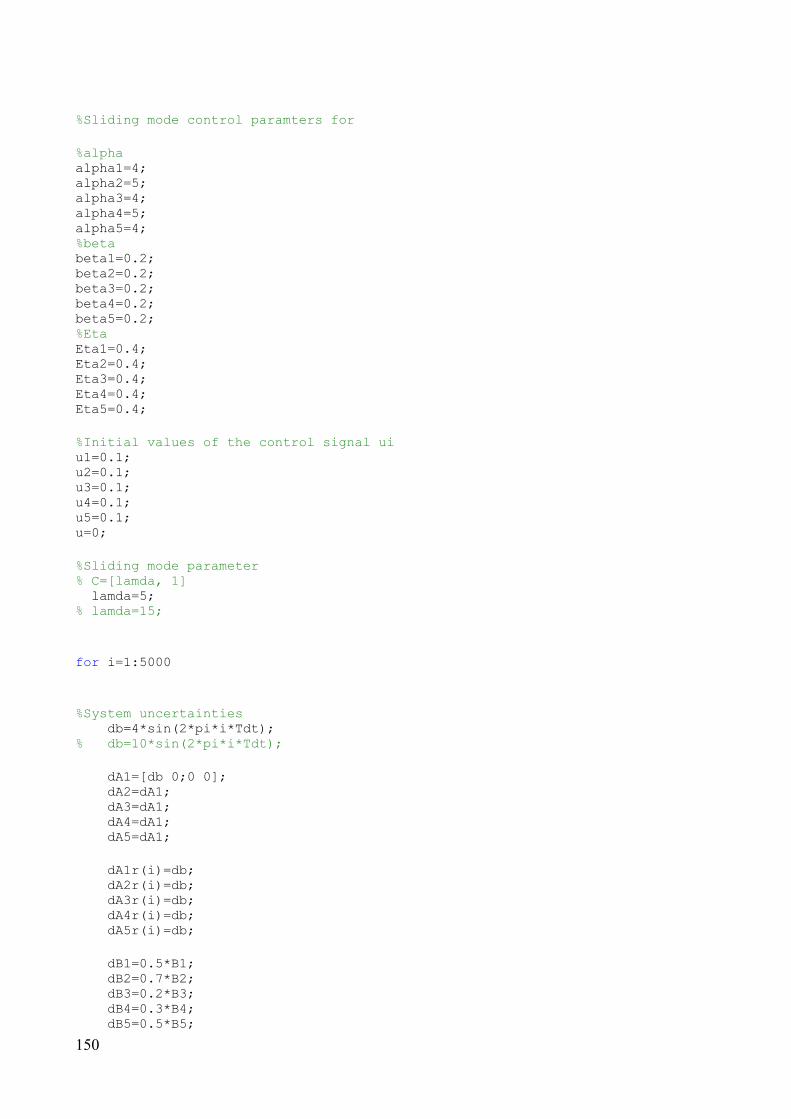
150

%Sliding mode control paramters for %alpha alpha1=4; alpha2=5; alpha3=4; alpha4=5; alpha5=4; %beta beta1=0.2; beta2=0.2; beta3=0.2; beta4=0.2; beta5=0.2; %Eta Eta1=0.4; Eta2=0.4; Eta3=0.4; Eta4=0.4; Eta5=0.4; %Initial values of the control signal ui u1=0.1; u2=0.1; u3=0.1; u4=0.1; u5=0.1; u=0; %Sliding mode parameter % C=[lamda, 1] lamda=5; % lamda=15; for i=1:5000 %System uncertainties db=4*sin(2*pi*i*Tdt); % db=10*sin(2*pi*i*Tdt); dA1=[db 0;0 0]; dA2=dA1; dA3=dA1; dA4=dA1; dA5=dA1; dA1r(i)=db; dA2r(i)=db; dA3r(i)=db; dA4r(i)=db; dA5r(i)=db; dB1=0.5*B1; dB2=0.7*B2; dB3=0.2*B3; dB4=0.3*B4; dB5=0.5*B5;

151

dB11r(i)=dB1(1); dB12r(i)=dB1(2); dB21r(i)=dB2(1); dB22r(i)=dB2(2); dB31r(i)=dB3(1); dB32r(i)=dB3(2); dB41r(i)=dB4(1); dB42r(i)=dB4(2); dB51r(i)=dB5(1); dB52r(i)=dB5(2); %x1 membership up3pi=1/(1+exp(-3*pi*(x(1)-pi/6))); un3pi=1/(1+exp(3*pi*(x(1)+pi/6))); ud0=1-up3pi-un3pi; up3g(i)=up3pi; un3g(i)=un3pi; ud0g(i)=ud0; %x2 membership up4=1/(1+exp(-3*pi*(x(2)-pi/3))); un4=1/(1+exp(3*pi*(x(2)+pi/3))); u0=1-up4-un4; up4g(i)=up4; un4g(i)=un4; u0g(i)=u0; %5 fuzzy rules r1=(u0*ud0); r2=max(ud0*up4,ud0*un4); r3=max(up3pi*u0,un3pi*u0); r4=max(up3pi*up4,un3pi*un4); r5=1-r1-r2-r3-r4; %Sliding variable s=x(2)+lamda*x(1); s1(i)=s; c=[lamda 1]; %Lyapunov function v1=0.5*s*s; v(i)=0.5*s*s; %Correction term if i==1 du1=0; du2=0; du3=0; du4=0; du5=0; sd1=0; sd2=0; sd3=0; sd4=0;

152

sd5=0; vd1=0; vd2=0; vd3=0; vd4=0; vd5=0; elseif i==2 du1=0; du2=0; du3=0; du4=0; du5=0; sd1=0; sd2=0; sd3=0; sd4=0; sd5=0; vd1=0; vd2=0; vd3=0; vd4=0; vd5=0; else %estimated vd % vd1=(3/2*v(i)-2*v(i-1)+0.5*v(i-2))/dt; vd1=(v(i)-v(i-1))/dt; du1=inv(c*B1)/s*(alpha1*(v(i))+beta1*(v(i-1))+Eta1*(vd1)); du2=inv(c*B2)/s*(alpha1*(v(i))+beta1*(v(i-1))+Eta1*(vd1)); du3=inv(c*B3)/s*(alpha1*(v(i))+beta1*(v(i-1))+Eta1*(vd1)); du4=inv(c*B4)/s*(alpha1*(v(i))+beta1*(v(i-1))+Eta1*(vd1)); du5=inv(c*B5)/s*(alpha1*(v(i))+beta1*(v(i-1))+Eta1*(vd1)); end %local control signal u1=u1-du1; u2=u2-du2; u3=u3-du3; u4=u4-du4; u5=u5-du5; %global matrix A = (r1*(A1+dA1)+r2*(A2+dA1)+r3*(A3+dA1)+r4*(A4+dA1)+r5*(A5+dA1)); B = (r1*(B1+dB1)+r2*(B2+dB2)+r3*(B3+dB3)+r4*(B4+dB4)+r5*(B5+dB5)); r=[r1 r2 r3 r4 r5]; %Membership function r1r(i)=r1; r2r(i)=r2; r3r(i)=r3; r4r(i)=r4; r5r(i)=r5; %Dominant control principle

153

for j=1:4 if r(j)>=r(j+1) rmax=r(j); r(j)=r(j+1); r(j+1)=rmax; else rmax=r(j+1); end end if rmax==r1 u=u1; elseif rmax==r2 u=u2; elseif rmax==r3 u=u3; elseif rmax==r4 u=u4; else u=u5; end uu(i)=u; %Lipschitz condition %Vd(t-tao) if i==1 %Vd(t-tao) vdL1=0; vdL2=0; vdL3=0; vdL4=0; vdL5=0; %Vd(t,t-tao) vdK1=0; vdK2=0; vdK3=0; vdK4=0; vdK5=0; Vleft(i)=0; Vright(i)=0; else %Vd(t-tao) vdL1=s1(i-1)*c*((A1+[dA1r(i-1) 0;0 0])*[x1(i-1) x2(i-1)]'+(B1+[dB11r(i-1);dB12r(i-1)])*uu(i-1)); vdL2=s1(i-1)*c*((A2+[dA2r(i-1) 0;0 0])*[x1(i-1) x2(i-1)]'+(B2+[dB21r(i-1);dB22r(i-1)])*uu(i-1)); vdL3=s1(i-1)*c*((A3+[dA3r(i-1) 0;0 0])*[x1(i-1) x2(i-1)]'+(B3+[dB31r(i-1);dB32r(i-1)])*uu(i-1)); vdL4=s1(i-1)*c*((A4+[dA4r(i-1) 0;0 0])*[x1(i-1) x2(i-1)]'+(B4+[dB41r(i-1);dB42r(i-1)])*uu(i-1)); vdL5=s1(i-1)*c*((A5+[dA5r(i-1) 0;0 0])*[x1(i-1) x2(i-1)]'+(B5+[dB51r(i-1);dB52r(i-1)])*uu(i-1));

154

vdLT=r1r(i-1)*vdL1+r2r(i-1)*vdL2+r3r(i-1)*vdL3+r4r(i-1)*vdL4+r5r(i-1)*vdL5; %Vd(t,t-tao) vdK1=s1(i)*c*((A1+dA1)*x+(B1+dB1)*uu(i-1)); vdK2=s1(i)*c*((A2+dA2)*x+(B2+dB2)*uu(i-1)); vdK3=s1(i)*c*((A3+dA3)*x+(B3+dB3)*uu(i-1)); vdK4=s1(i)*c*((A4+dA4)*x+(B4+dB4)*uu(i-1)); vdK5=s1(i)*c*((A5+dA5)*x+(B5+dB5)*uu(i-1)); vdKT=r1r(i)*vdK1+r2r(i)*vdK2+r3r(i)*vdK3+r4r(i)*vdK4+r5r(i)*vdK5; %|vd(t,t-tao)-Vd(t-tao)|<1/M|Vd(t-tao)| %M=50 Vleft(i)=abs(vdKT-vdLT); Vright(i)=(1/20)*abs(vd1); %estimation error err(i)=vdLT-vd1; end x=x+dt*(A*x+B*u); x1(i)=x(1); x2(i)=x(2); end t=0.001:0.001:5; figure(1) subplot (2,1,1),plot(t,s1); xlabel('Time t (sec) sampling period:0.001s') ylabel('The sliding mode variable s(t)') subplot (2,1,2),plot(t,uu); xlabel('Time t (sec) sampling period:0.001s') ylabel('The control input signal(N)') figure(2) subplot (2,1,1),plot(t,x1,'-'); xlabel('Time t (sec) sampling period:0.001s') ylabel('The system states x1(rad)') subplot (2,1,2),plot(t,x2,'-'); xlabel('Time t (sec) sampling period:0.001s') ylabel('The system states x2(rad/s)') figure (3) plot(t,uu); xlabel('Time t (sec) sampling period:0.001s') ylabel('The control input signal(N)') figure (4) plot(t,Vleft,'--',t,Vright,'-'); xlabel('Time t (sec) sampling period:0.001s') ylabel('Lipschitz-like condition (4.4.6)') legend('Left hand side of (4.4.6)','Right hand side of (4.4.6)');

155

1.3 Matlab code for Chapter 5 clear clc close all %Sampling time dt=0.001; Dt1=0.001; Dt2=0.001; Dt3=0.001; %system A, system B and system C %system parameters %system A A11=[0 1;-2 3]; A12=[0 1;-2.4 3.3]; A13=[0 1;-3 4]; B1=[0;1]; D1=[1;0]; %system B A21=[0 1;-3 3]; A22=[0 1;-3.4 3.1]; B2=[0;1]; D2=D1; %system C A31=[0 1;-6 5.5]; A32=[0 1;-6.2 5.8]; B3=[0;1]; D3=D1; %Initial state value x11=0.2; x12=-0.5; x21=-0.2; x22=-0.1; x31=0.2; x32=-0.1; x1=[x11 x12]'; x2=[x21 x22]'; x3=[x31 x32]'; %Initial control input %For global fuzzy model u1=0.1; u2=0.1; u3=0.1; %For local linear model %system A u11=0.1; u12=0.1; u13=0.1;

156

%system B u21=0.1; u22=0.1; %system C u31=0.1; u32=0.1; %Reference Signal xr1=[0;0]; xr2=[0;0]; xr3=[0;0]; %Reference signal ArX1=[0 1;-10 -10]; ArX2=ArX1; ArX3=ArX1; Br=[0;1] xr=[0;0]; %control gain alpha11=0; alpha12=alpha11; alpha13=alpha11; beta11=0; beta12=beta11; beta13=beta11; eta11=0; eta12=eta11; eta13=eta11; alpha21=0; alpha22=alpha21; beta21=0; beta22=beta21; eta21=0; eta22=eta21; alpha31=0; alpha32=alpha31; beta31=0; beta32=beta31; eta31=0; eta32=eta31; %sliding mode variable lamda=10; for i=1:20000 %Reference signal R1=[0; 10*cos(0.5*i*Dt1)];

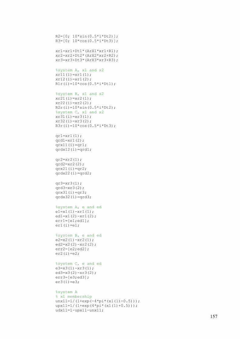
157

R2=[0; 10*sin(0.5*i*Dt2)]; R3=[0; 10*cos(0.5*i*Dt3)]; xr1=xr1+Dt1*(ArX1*xr1+R1); xr2=xr2+Dt2*(ArX2*xr2+R2); xr3=xr3+Dt3*(ArX3*xr3+R3); %system A, x1 and x2 xr11(i)=xr1(1); xr12(i)=xr1(2); R1r(i)=10*cos(0.5*i*Dt1); %system B, x1 and x2 xr21(i)=xr2(1); xr22(i)=xr2(2); R2r(i)=10*sin(0.5*i*Dt2); %system C, x1 and x2 xr31(i)=xr3(1); xr32(i)=xr3(2); R3r(i)=10*cos(0.5*i*Dt3); qr1=xr1(1); qrd1=xr1(2); qrx11(i)=qr1; qrdx12(i)=qrd1; qr2=xr2(1); qrd2=xr2(2); qrx21(i)=qr2; qrdx22(i)=qrd2; qr3=xr3(1); qrd3=xr3(2); qrx31(i)=qr3; qrdx32(i)=qrd3; %system A, e and ed e1=x1(1)-xr1(1); ed1=x1(2)-xr1(2); err1=[e1;ed1]; er1(i)=e1; %system B, e and ed e2=x2(1)-xr2(1); ed2=x2(2)-xr2(2); err2=[e2;ed2]; er2(i)=e2; %system C, e and ed e3=x3(1)-xr3(1); ed3=x3(2)-xr3(2); err3=[e3;ed3]; er3(i)=e3; %system A % x1 membership unx11=1/(1+exp(-4*pi*(x1(1)-0.5))); upx11=1/(1+exp(4*pi*(x1(1)+0.5))); udx11=1-upx11-unx11;

158

% x2 membership unx12=1/(1+exp(-4*pi*(x1(2)-0.5))); upx12=1/(1+exp(4*pi*(x1(2)+0.5))); udx12=1-upx12-unx12; %system B % x1 membership unx21=1/(1+exp(-4*pi*(x2(1)-0.5))); upx21=1/(1+exp(4*pi*(x2(1)+0.5))); udx21=1-upx21-unx21; % x2 membership unx22=1/(1+exp(-4*pi*(x2(2)-0.5))); upx22=1/(1+exp(4*pi*(x2(2)+0.5))); udx22=1-upx22-unx22; %system C % x1 membership unx31=1/(1+exp(-2*pi*(x3(1)-pi/3))); upx31=1/(1+exp(2*pi*(x3(1)+pi/3))); udx31=1-upx31-unx31; % x2 membership unx32=1/(1+exp(-2*pi*(x3(2)-pi/3))); upx32=1/(1+exp(2*pi*(x3(2)+pi/3))); udx32=1-upx32-unx32; % 7 fuzzy rules %system A %rule 1 r11=(udx11*udx12); %rule 2 r12=max(udx11*unx12,udx11*upx12); %rule 3 r13=1-r11-r12; %system B %rule 1 r21=(udx21*udx22); %rule 2 r22=1-r21; %system C %rule 1 r31=(udx31*udx32); %rule 2 r32=1-r31; %sliding variable s1,s2,s3 %s1 s1=ed1+lamda*e1; s1r(i)=s1; c1=[lamda/1 1/1]; %v1(i)=0.5*s1*s1; %s2 s2=ed2+lamda*e2; s2r(i)=s2;

159

%c2=[15 1]; c2=[lamda/1 1/1]; %v2(i)=0.5*s2*s2; %s3 s3=ed3+lamda*e3; s3r(i)=s3; c3=[lamda/1 1/1]; %v3(i)=0.5*s3*s3; % local sliding mode learning controller %Correction term if i==1 %system A du11=0; du12=0; du13=0; %system B du21=0; du22=0; %system C du31=0; du32=0; v1(i)=0.5*s1*s1; v2(i)=0.5*s2*s2; v3(i)=0.5*s3*s3; else %sd v1(i)=0.5*s1*s1; v2(i)=0.5*s2*s2; v3(i)=0.5*s3*s3; %system A vd11=(v1(i)-v1(i-1))/dt; vd12=(v1(i)-v1(i-1))/dt; vd13=(v1(i)-v1(i-1))/dt; %system B vd21=(v2(i)-v2(i-1))/dt; vd22=(v2(i)-v2(i-1))/dt; %system C vd31=(v3(i)-v3(i-1))/dt; vd32=(v3(i)-v3(i-1))/dt; %adaptation laws alpha11=alpha11+dt*(20*abs(v1(i))); beta11=beta11+dt*(0.01*abs(vd11)); eta11=eta11+dt*(0.1*abs(vd11)); alpha21=alpha21+dt*(20*abs(v2(i))); beta21=beta21+dt*(0.01*abs(vd11)); eta21=eta21+dt*(0.1*abs(vd21)); alpha31=alpha31+dt*(20*abs(v3(i))); beta31=beta31+dt*(0.01*abs(vd11)); eta31=eta31+dt*(0.1*abs(vd31));

160

alpha12=alpha11; alpha13=alpha11; beta12=beta11; beta13=beta11; eta12=eta11; eta13=eta11; alpha22=alpha21; beta22=beta21; eta22=eta21; alpha32=alpha31; beta32=beta31; eta32=eta31; %system A du11=inv(c1*B1)/s1*(alpha11*v1(i)+beta11*abs(vd11)+eta11*vd11); du12=inv(c1*B1)/s1*(alpha12*v1(i)+beta12*abs(vd12)+eta12*vd12); du13=inv(c1*B1)/s1*(alpha13*v1(i)+beta13*abs(vd13)+eta13*vd13); %system B du21=inv(c2*B2)/s2*(alpha21*v2(i)+beta21*abs(vd21)+eta21*vd21); du22=inv(c2*B2)/s2*(alpha22*v2(i)+beta22*abs(vd21)+eta22*vd22); %system C du31=inv(c3*B3)/s3*(alpha31*v3(i)+beta31*abs(vd31)+eta31*vd31); du32=inv(c3*B3)/s3*(alpha32*v3(i)+beta32*abs(vd31)+eta32*vd32); end %local control input u11=u11-du11; u12=u12-du12; u13=u13-du13; u21=u21-du21; u22=u22-du22; u31=u31-du31; u32=u32-du32; % global matrix A1 = (r11*(A11)+r12*(A12)+r13*(A13)); A2 = (r21*(A21)+r22*(A22)); A3 = (r31*(A31)+r32*(A32)); %internal connection term

161

f112=0.5*sin(2*pi*x2*dt); f212=f112; f312=f112; f113=0.5*sin(2*pi*x3*dt); f213=f113; f313=f113; f121=0.6*sin(2*pi*x1*dt); f221=f121; f123=0.6*sin(2*pi*x3*dt); f223=f123; f131=0.5*sin(2*pi*x1*dt); f231=f131; f132=0.5*sin(2*pi*x2*dt); f232=f132; Ain1=r11*(f112+f113)+r12*(f212+f213)+r13*(f312+f313); Ain2=r21*(f121+f123)+r22*(f221+f223); Ain3=r31*(f131+f132)+r32*(f231+f232); rx1=[r11 r12 r13]; rx2=[r21 r22]; rx3=[r31 r32]; %dominant control principle for j=1:2 if rx1(j)>=rx1(j+1) rmaxx1=rx1(j); rx1(j)=rx1(j+1); rx1(j+1)=rmaxx1; else rmaxx1=rx1(j+1); end end %global control input if rmaxx1==r11 u1=u11; elseif rmaxx1==r12 u1=u12; else u1=u13; end if rx2(1)>=rx2(2) u2=u21; else u2=u22; end if rx3(1)>=rx3(2) u3=u31;

162

else u3=u32; end u1 = (r11*(u11)+r12*(u12)+r13*(u13)); u2 = (r21*(u21)+r22*(u22)); u3 = (r31*(u31)+r32*(u32)); uu1(i)=u1; uu2(i)=u2; uu3(i)=u3; x1=x1+dt*(A1*x1+Ain1+(B1)*u1); x2=x2+dt*(A2*x2+Ain2+(B2)*u2); x3=x3+dt*(A3*x3+Ain3+(B3)*u3); x11r(i)=x1(1); x12r(i)=x1(2); x21r(i)=x2(1); x22r(i)=x2(2); x31r(i)=x3(1); x32r(i)=x3(2); alpha1kr(i)=alpha11; beta1kr(i)=beta11; eta1kr(i)=eta11; alpha2kr(i)=alpha21; beta2kr(i)=beta21; eta2kr(i)=eta21; alpha3kr(i)=alpha31; beta3kr(i)=beta31; eta3kr(i)=eta31; end t=0.001:0.001:20; figure(1) subplot (2,1,1),plot(t,x11r,'-',t,xr11,'--'); xlabel('Time t (sec) sampling period:0.001s') title('The system state x11(rad)and reference state xr11(rad)') legend('x11','x11 reference signal'); subplot (2,1,2),plot(t,x12r,'-',t,xr12,'--'); xlabel('Time t (sec) sampling period:0.001s') title('The system state x12(rad/s)and reference state xr12(rad/s)') legend('x12','x12 reference signal'); figure(2) subplot (2,1,1),plot(t,x21r,'-',t,xr21,'--'); xlabel('Time t (sec) sampling period:0.001s')

163

title('The system state x21(rad)and reference state xr21(rad)') legend('x21','x21 reference signal'); subplot (2,1,2),plot(t,x22r,'-',t,xr22,'--'); xlabel('Time t (sec) sampling period:0.001s') title('The system state x22(rad/s)and reference state xr22(rad/s)') legend('x22','x22 reference signal'); figure(3) subplot (2,1,1),plot(t,x31r,'-',t,xr31,'--'); xlabel('Time t (sec) sampling period:0.001s') title('The system state x31(rad)and reference state xr31(rad)') legend('x31','x31 reference signal'); subplot (2,1,2),plot(t,x32r,'-',t,xr32,'--'); xlabel('Time t (sec) sampling period:0.001s') title('The system state x32(rad/s)and reference state xr32(rad/s)') legend('x32','x32 reference signal'); figure(4) plot(t,uu1,'-',t,uu2,'--',t,uu3,'-.'); xlabel('Time t (sec) sampling period:0.001s') title('The global fuzzy control input u1,u2 and u3') figure(5) plot(t,alpha1kr,'-',t,beta1kr,'--',t,eta1kr,'-.'); xlabel('Time t (sec) sampling period:0.001s') title('The adaptation parameters for S1') legend('alpha1k','beta1k','eta1k'); AXIS([0 3 0 1.5]) figure(6) plot(t,alpha2kr,'-',t,beta2kr,'--',t,eta2kr,'-.'); xlabel('Time t (sec) sampling period:0.001s') title('The adaptation parameters for S2') legend('alpha2k','beta2k','eta2k'); AXIS([0 3 0 3.5]) figure(7) plot(t,alpha3kr,'-',t,beta3kr,'--',t,eta3kr,'-.'); xlabel('Time t (sec) sampling period:0.001s') title('The adaptation parameters for S3') legend('alpha3k','beta3k','eta3k'); AXIS([0 3 0 2.5]) figure(8) plot(t,s1r,'-'); xlabel('Time t (sec) sampling period:0.001s') title('The sliding variable for S1') AXIS([0 3 -0.5 1.6]) figure(9) plot(t,s2r,'-'); xlabel('Time t (sec) sampling period:0.001s')

164

title('The sliding variable for S2') AXIS([0 3 -2.5 0.5]) figure(10) plot(t,s3r,'-'); xlabel('Time t (sec) sampling period:0.001s') title('The sliding variable for S3') AXIS([0 3 -0.5 2])

165

List of Publications

1. F. Tay, Z. Man, Z. Cao, S. Khoo, and C. P. Tan, “Sliding mode-like learning

control for SISO complex systems with T–S fuzzy models,” International

Journal of Modelling, Identification & Control, vol.16, no.4, pp.317-326, 2012.

2. D. M. Tuan, Z. Man, C. Zhang, H. Wang, and F. Tay, “Robust sliding mode

learning control for steer-by-wire systems,” accepted by IEEE Transactions on

Vehicular Technology, 2013.

3. Z. Man, S. Khoo, X. Yu, C. Miao, J. Jin, and F. Tay, “A new design of sliding

mode control systems,” in Sliding Modes after the First Decade of the 21st

Century, vol. 412. M. Thoma, F. Allgöwer, and M. Morari, Ed.

Berlin/Heidelberg: Springer, pp.151-167, 2012.

4. F. Tay, Z. Man, and Z. Cao, “Sliding mode learning control for SISO complex

systems with T-S fuzzy models,” The 37th IEEE Conference on Industrial

Electronics Society (IECON), pp.751-756, 2011.

5. F. Tay, Z. Man, Z. Cao, J. Jin, and S. Y. Khoo, “A robust learning control for

SISO nonlinear systems with T-S fuzzy model,” The 12th IEEE Conference on

Control, Automation, Robotics &Vision (ICARCV), pp,492-497, 2012.

6. F. Tay, Z. Man, J. Jin, S. Khoo, J. Zheng, and H. Wang, “Sliding mode based

learning control for interconnected systems,” to appear in the Proc. of The 8th

IEEE Conference on Industrial Electronics and Applications (ICIEA), 2013.

166

7. F. Tay, Z. Man, J. Jin, and D. M. Tuan, “Sliding mode learning control of fuzzy

uncertain continuous-time SISO system,” to be submitted to Fuzzy Sets and

Systems.

8. F. Tay, Z. Man, J. Jin, S. Khoo, J. Zheng, and D. M. Tuan, “Sliding mode

learning fuzzy model reference tracking control for a class of large-scale system

with adaptive estimation,” to be submitted to IEEE Transactions on Fuzzy

Systems.

Sliding mode-based learning control for complex systems … · Sliding Mode-based Learning Control...

Documents

Transcript of Sliding mode-based learning control for complex systems … · Sliding Mode-based Learning Control...