Slides Set 11 (part a)dechter/courses/ics-276/spring...Slides Set 11 (part a): Rina Dechter...

Algorithms for Reasoning with graphical models

Slides Set 11 (part a):

Rina Dechter

slides11a 828X 2019

Sampling Techniques for Probabilistic and Deterministic Graphical models

(Reading” Darwiche chapter 15, related papers)

Sampling Techniques for Probabilistic and Deterministic Graphical models

ICS 276, Spring 2018Bozhena Bidyuk

Reading” Darwiche chapter 15, related papers

slides11a 828X 2019

Overview

1. Basics of sampling2. Importance Sampling3. Markov Chain Monte Carlo: Gibbs Sampling4. Sampling in presence of Determinism 5. Rao‐Blackwellisation, cutset sampling

slides11a 828X 2019

Sum-Inference

Max-Inference

Mixed-Inference

Types of queries

• NP-hard: exponentially many terms• We will focus on approximation algorithms

– Anytime: very fast & very approximate ! Slower & more accurate

Harder

slides10 828X 2019

Monte Carlo estimators• Most basic form: empirical estimate of probability

• Relevant considerations– Able to sample from the target distribution p(x)?– Able to evaluate p(x) explicitly, or only up to a constant?

• “Any‐time” properties– Unbiased estimator,

or asymptotically unbiased,

– Variance of the estimator decreases with m

slides11a 828X 2019

Monte Carlo estimators• Most basic form: empirical estimate of probability

• Central limit theorem– p(U) is asymptotically Gaussian:

• Finite sample confidence intervals– If u(x) or its variance are bounded, e.g.,

probability concentrates rapidly around the expectation:

m=1: m=5: m=15:

slides11a 828X 2019

slides11a 828X 2019

A Sample• Given a set of variables X={X1,...,Xn}, a sample, denoted by St is an instantiation of all variables:

),...,,( tn

ttt xxxS 21

slides11a 828X 2019

How to Draw a Sample ?Univariate Distribution

• Example: Given random variable X having domain {0, 1} and a distribution P(X) = (0.3, 0.7).

• Task: Generate samples of X from P.• How?

– draw random number r [0, 1]– If (r < 0.3) then set X=0– Else set X=1

slides11a 828X 2019

How to Draw a Sample?Multi‐Variate Distribution

• Let X={X1,..,Xn} be a set of variables• Express the distribution in product form

• Sample variables one by one from left to right, along the ordering dictated by the product form.

• Bayesian network literature: Logic sampling or Forward Sampling.

),...,|(...)|()()( 11121 nn XXXPXXPXPXP

slides11a 828X 2019

Sampling in Bayes nets (Forward Sampling)• No evidence: “causal” form makes sampling easy

– Follow variable ordering defined by parents– Starting from root(s), sample downward– When sampling each variable, condition on values of parents

A B

C

D Sample:

[e.g., Henrion 1988]

slides11a 828X 2019

Froward Sampling: No Evidence (Henrion1988)

Input: Bayesian networkX= {X1,…,XN}, N‐ #nodes, T ‐ # samples

Output: T samples Process nodes in topological order – first process the

ancestors of a node, then the node itself:1. For t = 0 to T2. For i = 0 to N3. Xi sample xit from P(xi | pai)

slides11a 828X 2019

Forward Sampling w/ EvidenceInput: Bayesian network

X= {X1,…,XN}, N‐ #nodesE – evidence, T ‐ # samples

Output: T samples consistent with E1. For t=1 to T2. For i=1 to N3. Xi sample xit from P(xi | pai)4. If Xi in E and Xi xi, reject sample:5. Goto Step 1.

slides11a 828X 2019

Forward Sampling (example)

X1

X4

X2 X3

)( 1xP

)|( 12 xxP

),|( 324 xxxP

)|( 13 xxP

)|( from Sample 5.otherwise 1, fromstart and

samplereject 0, If .4)|( from Sample .3)|( from Sample .2

)( from Sample .1 sample generate//

0 :Evidence

3,244

3

133

122

11

3

xxxPx

xxxPxxxPx

xPxk

X

slides11a 828X 2019

Expected value: Given a probability distribution P(X) and a function g(X) defined over a set of variables X = {X1, X2, … Xn}, the expected value of g w.r.t. P is

Variance: The variance of g w.r.t. P is:

How to answer queries with sampling?Expected value and Variance

)()()]([ xPxgxgEx

P

)()]([)()]([ 2 xPxgExgxgVarx

PP

slides11a 828X 2019

Many queries can be phrased as computing expectation of some functions

Monte Carlo Estimate

• Estimator: – An estimator is a function of the samples.– It produces an estimate of the unknown parameter of the sampling distribution.

T

tt

P

SgT

g

P

1

T21

1

:bygiven is [g(x)]E of estimate carlo Monte the , fromdrawn S ,S ,S samples i.i.d.Given

)(ˆ

slides11a 828X 2019

Example: Monte Carlo estimate• Given:

– A distribution P(X) = (0.3, 0.7).– g(X) = 40 if X equals 0

= 50 if X equals 1.• Estimate EP[g(x)]=(40x0.3+50x0.7)=47.• Generate k samples from P: 0,1,1,1,0,1,1,0,1,0

4610

650440

150040

samplesXsamplesXsamplesg

#)(#)(#ˆ

slides11a 828X 2019

Bayes Nets with Evidence• Estimating posterior probabilities, P[A = a | E=e]?

• Rejection sampling– Draw x ~ p(x), but discard if E e– Resulting samples are from p(x | E=e); use as before– Problem: keeps only P[E=e] fraction of the samples!– Performs poorly when evidence probability is small

• Estimate the ratio: P[A=a,E=e] / P[E=e]– Two estimates (numerator & denominator)– Good finite sample bounds require low relative error!– Again, performs poorly when evidence probability is small– What bounds can we get?

slides11a 828X 2019

slides11a 828X 2019

absolute

slides11a 828X 2019

Bayes Nets With Evidence• Estimating the probability of evidence, P[E=e]:

– Finite sample bounds: u(x) ∈ [0,1]

– Relative error bounds [Dagum & Luby 1997]

[e.g., Hoeffding]

What if the evidence is unlikely? P[E=e]=1e‐6 ) could estimate U = 0!

slides11a 828X 2019

So, if U, the probability of evidence is very small we would need many many samplesTht are not rejected.

Overview

1. Basics of sampling2. Importance Sampling3. Markov Chain Monte Carlo: Gibbs Sampling4. Sampling in presence of Determinism 5. Rao‐Blackwellisation, cutset sampling

slides11a 828X 2019

Importance Sampling: Main Idea

• Express query as the expected value of a random variable w.r.t. to a distribution Q.

• Generate random samples from Q.• Estimate the expected value from the generated samples using a monte carloestimator (average).

slides11a 828X 2019

Importance Sampling• Basic empirical estimate of probability:

• Importance sampling:

slides11a 828X 2019

Importance Sampling• Basic empirical estimate of probability:

• Importance sampling:

“importance weights”

slides11a 828X 2019

slides11a 828X 2019

Estimating P(E) and P(X|e)

Importance Sampling For P(e)

)(,)()(ˆ

:

)]([)(),(

)()(),(),()(

)(),(

,\

ZQzwT

eP

zwEzQezPE

zQzQezPezPeP

zQezP

EXZLet

tT

t

t

QQzz

z where1estimate Carlo Monte

:as P(e) rewritecan weThen,00

satisfying on,distributi (proposal) a be Q(Z)Let

1

slides11a 828X 2019

Properties of IS Estimate of P(e) • Convergence: by law of large numbers

• Unbiased.

• Variance:

Tfor )()(1)(ˆ ..

1ePzw

TeP saT

ii

T

zwVarzw

TVarePVar QN

ii

QQ

)]([)(1)(ˆ

1

)()](ˆ[ ePePEQ

slides11a 828X 2019

Properties of IS Estimate of P(e)• Mean Squared Error of the estimator

TxwVar

ePVar

ePVarePEeP

ePePEePMSE

Q

Q

QQ

QQ

)]([

)(ˆ)(ˆ)](ˆ[)(

)()(ˆ)(ˆ

2

2

This quantity enclosed in the brackets is zero because the expected value of the

estimator equals the expected value of g(x)

slides11a 828X 2019

slides11a 828X 2019

Estimating P(E) and P(X|e)

Estimating P(Xi|e)

)|()|(E:biased is Estimate

,

,

)(ˆ),(ˆ

)|(:estimate Ratio

IS.by r denominato andnumerator Estimate :Idea)(),(

)(),()(

),(

),()(

)(),()|(

otherwise. 0 and xcontains z if 1 is which function, delta-dirac a be (z)Let

T

1k

T

1k

ixi

exPexP

e)w(z

e))w(z(z

ePexPexP

zQezPE

zQezPz

E

ezP

ezPz

ePexPexP

ii

k

kkx

ii

Q

xQ

z

zx

ii

i

i

i

slides11a 828X 2019

Properties of the IS estimator for P(Xi|e)

• Convergence: By Weak law of large numbers

• Asymptotically unbiased

• Variance– Harder to analyze– Liu suggests a measure called “Effective sample size”

T as )|()|( exPexP ii

)|()]|([lim exPexPE iiPT

slides11a 828X 2019

Effective Sample Size

possible. as small as bemust weights theof variance theTherefore,Q. from samples T)ESS(Q, worth are P from samples T Thus

),()]|([)]|(ˆ[

)]([var1),(:

1ˆ

:using e)|P(x estimatecan wee),|P(z from samplesGiven

)|()()|(

1

i

TQESST

exPVarexPVar

zwTTQESSDefine

)(zgT

|e)(xP

ezPzgexP

iQ

iP

Q

T

j

txi

zxi

i

i

Ideal estimator

Measures how much the estimator deviates from the ideal one.

slides11a 828X 2019

Generating Samples From Q

• No restrictions on “how to”• Typically, express Q in product form:

– Q(Z)=Q(Z1)xQ(Z2|Z1)x….xQ(Zn|Z1,..Zn‐1)

• Sample along the order Z1,..,Zn• Example:

– Z1Q(Z1)=(0.2,0.8)– Z2 Q(Z2|Z1)=(0.1,0.9,0.2,0.8)– Z3 Q(Z3|Z1,Z2)=Q(Z3)=(0.5,0.5)

slides11a 828X 2019

Summary: IS for Common Queries• Partition function

– Ex: MRF, or BN with evidence

– Unbiased; only requires evaluating unnormalized function f(x)

• General expectations wrt p(x) / f(x)?– E.g., marginal probabilities, etc.

Only asymptotically unbiased…

Estimate separately

slides11a 828X 2019

More on Properties of IS • Importance sampling:

• IS is unbiased and fast if q(.) is easy to sample from

• IS can be lower variance if q(.) is chosen well– Ex: q(x) puts more probability mass where u(x) is large– Optimal: q(x) ∝ |u(x) p(x)|

• IS can also give poor performance– If q(x) << u(x) p(x): rare but very high weights!– Then, empirical variance is also unreliable!– For guarantees, need to analytically bound weights / variance…

How to get a good proposal?

Outline

• Definitions and Background on Statistics• Theory of importance sampling• Likelihood weighting• State‐of‐the‐art importance sampling techniques

slides11a 828X 2019

Likelihood Weighting(Fung and Chang, 1990; Shachter and Peot, 1990)

Works well for likely evidence!

“Clamping” evidence+logic sampling+weighing samples by evidence likelihood

Is an instance of importance sampling!

slides11a 828X 2019

Likelihood Weighting: Sampling

e e e e e

e e e e

Sample in topological order over X !

Clamp evidence, Sample xi P(Xi|pai), P(Xi|pai) is a look‐up in CPT!

slides11a 828X 2019

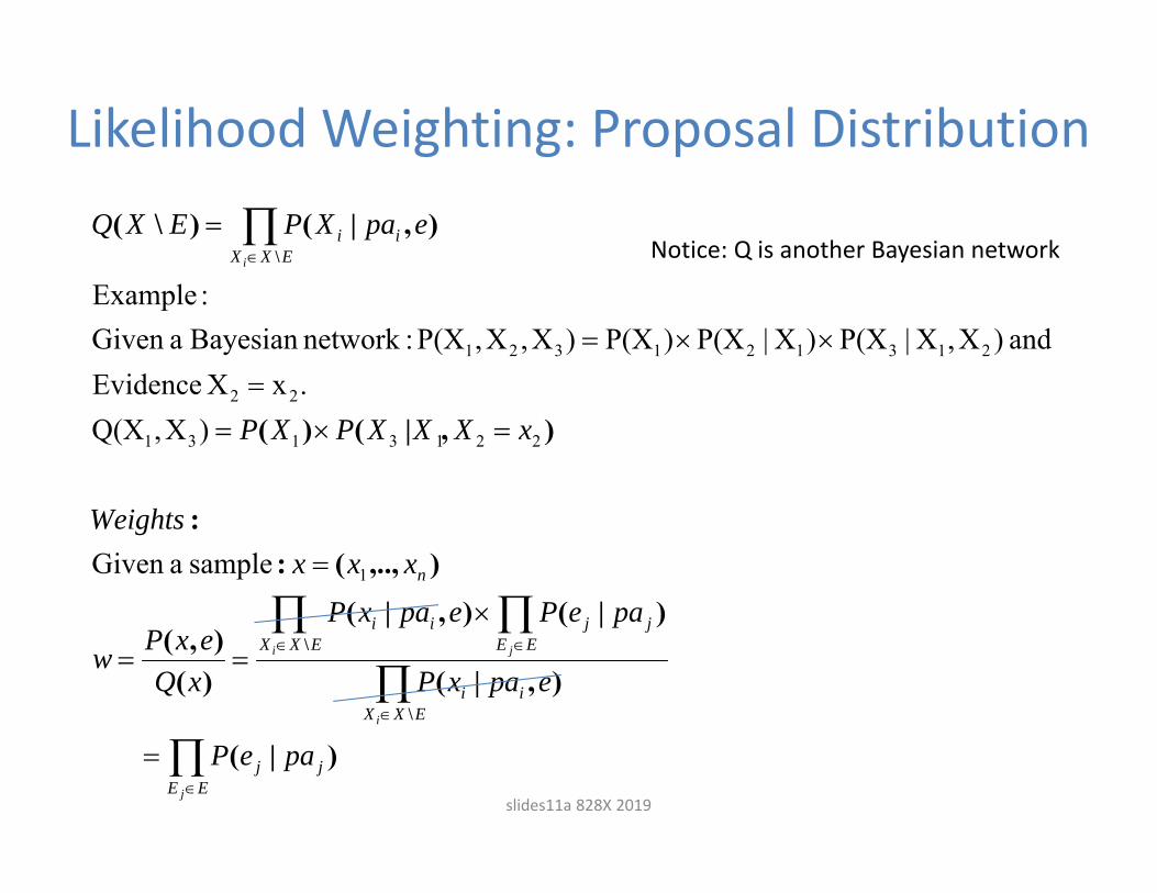
Likelihood Weighting: Proposal Distribution

EEjj

EXXii

EXX EEjjii

n

EXXii

j

i

i j

i

paeP

epaxP

paePepaxP

xQexPw

xxxWeights

xXXXPXP

epaXPEXQ

)|(

),|(

)|(),|(

)(),(

),..,(::

),|()(

),|()\(

\

\

\

sample aGiven

)X,Q(X.xX Evidence

and )X,X|P(X)X|P(X)P(X)X,X,P(X :networkBayesian aGiven :Example

1

2213131

22

213121321

Notice: Q is another Bayesian network

slides11a 828X 2019

Likelihood Weighting: Estimates

T

t

twT

eP1

)(1)(ˆEstimate P(e):

otherwise zero equals and xif 1)(

)(

)(ˆ),(ˆ

)|(ˆ

i)(

1

)(

)(

1

)(

ti

tx

T

t

t

tx

T

t

t

ii

xxg

w

xgw

ePexPexP

i

i

Estimate Posterior Marginals:

slides11a 828X 2019

Properties of Likelihood Weighting

• Converges to exact posterior marginals• Generates Samples Fast• Sampling distribution is close to prior (especially if E Leaf Nodes)

• Increasing sampling varianceConvergence may be slowMany samples with P(x(t))=0 rejected

slides11a 828X 2019

Outline

• Definitions and Background on Statistics• Theory of importance sampling• Likelihood weighting• State‐of‐the‐art importance sampling techniques

slides11a 828X 2019

Proposal selection• One should try to select a proposal that is as close as possible to the posterior distribution.

)|()(

)()(),(

estimator variance-zero a have to,0)()(),(

)()()(),(1)]([

)(ˆ2

ezPzQ

zQePezP

ePzQezP

zQePzQezP

NTzwVar

ePVarZz

QQ

slides11a 828X 2019

Proposal Distributions used in Literature

• AIS‐BN (Adaptive proposal) • Cheng and Druzdzel, 2000

• Iterative Belief Propagation • Changhe and Druzdzel, 2003

• Iterative Join Graph Propagation (IJGP) and variable ordering • Gogate and Dechter, 2005

slides11a 828X 2019

Perfect sampling using Bucket Elimination

• Algorithm:– Run Bucket elimination on the problem along an ordering o=(XN,..,X1).

– Sample along the reverse ordering: (X1,..,XN)– At each variable Xi, recover the probability P(Xi|x1,...,xi‐1) by referring to the bucket.

slides11a 828X 2019

Exact Sampling using Bucket Elimination

• Algorithm:– Run Bucket elimination on the problem along an ordering o=(X1,..,XN).

– Sample along the reverse ordering– At each branch point, recover the edge probabilities by performing a constant‐time table lookup!

– Complexity: O(Bucket‐elimination)+O(M*n)• M is the number of solution samples and n is the number of variables

slides11a 828X 2019

Downward message normalizes bucket;ratio is a conditional distribution

E:

C:

D:

B:

A:

How to sample from a Markov network?Exact sampling via inference

• Draw samples from P[A|E=e] directly?– Model defines un‐normalized p(A,…,E=e)– Build (oriented) tree decomposition & sample

Z

Work: O(exp(w)) to build distributionO(n d) to draw each sampleslides11a 828X 2019

Bucket Elimination )0,()0|( eaPeaP

debc

cbePbadPacPabPaPeaP,0,,

),|(),|()|()|()()0,(

dc b e

badPcbePabPacPaP ),|(),|()|()|()(0

Elimination Order: d,e,b,cQuery:

D:

E:

B:

C:

A:

d

D badPbaf ),|(),(),|( badP

),|( cbeP ),|0(),( cbePcbfE

b

EDB cbfbafabPcaf ),(),()|(),(

)()()0,( afApeaP C)(aP

)|( acP c

BC cafacPaf ),()|()(

)|( abP

D,A,B E,B,C

B,A,C

C,A

A

),( bafD ),( cbfE

),( cafB

)(afC

AA

DD EE

CCBB

Bucket TreeD E

B

C

A

Original Functions Messages

Time and space exp(w*) slides11a 828X 2019

slides11a 828X 2019

Bucket elimination (BE)

b

Elimination operator

P(e)

bucket B:

P(a)

P(C|A)

P(B|A) P(D|B,A) P(e|B,C)

bucket C:

bucket D:

bucket E:

bucket A:

B

C

D

E

A

e)(A,hD

(a)hE

e)C,D,(A,hB

e)D,(A,hC

AA

DD EE

CCBB

slides11a 828X 2019

Sampling from the output of BE(Dechter 2002)

bucket B:

P(A)

P(C|A)

P(B|A) P(D|B,A) P(e|B,C)

bucket C:

bucket D:

bucket E:

bucket A:

e)(A,hD

(A)hE

e)C,D,(A,hB

e)D,(A,hC

Q(A)aA:(A)hP(A)Q(A) E

Sample

ignore :bucket Evidence

e)D,(a,he)a,|Q(Dd D :Samplebucket in the aASet

C

e)C,d,(a,h)|(d)e,a,|Q(C cC :Samplebucket thein dDa,ASet

B

ACP

),|(),|()|(d)e,a,|Q(Bb B:Samplebucket thein cCd,Da,ASet

cbePaBdPaBP

slides11a 828X 2019 57

Mini‐Bucket Elimination

bucket A:

bucket E:

bucket D:

bucket C:

bucket B:

ΣB

P(B|A) P(D|B,A)

hE(A)

hB(A,D)

P(e|B,C)

Mini-buckets

ΣB

P(C|A) hB(C,e)

hD(A)

hC(A,e)

Approximation of P(e)

Space and Time constraints:Maximum scope size of the new function generated should be bounded by 2

BE generates a function having scope size 3. So it cannot be used.

P(A)

slides11a 828X 2019 58

Sampling from the output of MBE

bucket A:

bucket E:

bucket D:

bucket C:

bucket B: P(B|A) P(D|B,A)

hE(A)

hB(A,D)

P(e|B,C)

P(C|A) hB(C,e)

hD(A)

hC(A,e) Sampling is same as in BE‐sampling except that now we construct Q from a randomly selected “mini‐bucket”

IJGP‐Sampling (Gogate and Dechter, 2005)

• Iterative Join Graph Propagation (IJGP)– A Generalized Belief Propagation scheme (Yedidiaet al., 2002)

• IJGP yields better approximations of P(X|E) than MBE (Dechter, Kask and Mateescu, 2002)

• Output of IJGP is same as mini‐bucket “clusters”

• Currently one of the best performing IS scheme!

slides11a 828X 2019

Example: IJGP‐Sampling

• Run IJGP

A

B

C

D

E Sampling OrderApprox #Solutions (i=2)

CD

AD

BCD BE

DE

ABE

E

A

C

E

DB

slides11a 828X 2019

Current Research Question

• Given a Bayesian network with evidence or a Markov network representing function P, generate another Bayesian network representing a function Q (from a family of distributions, restricted by structure) such that Q is closest to P.

• Current approaches– Mini‐buckets– Ijgp– Both

• Experimented, but need to be justified theoretically.

slides11a 828X 2019

Algorithm: Approximate Sampling

1) Run IJGP or MBE2) At each branch point compute the edge

probabilities by consulting output of IJGP or MBE

• Rejection Problem:– Some assignments generated are non solutions

slides11a 828X 2019

k)(ˆ

Re

')(Q Update

)(N1)(ˆe)(EP̂

Q z,...,z samples Generate dok to1iFor

0)(ˆ))(|(...))(|()()(Q Proposal Initial

1k

1

N1

2211

eEPturn

EndQQkQ

zweEP

from

eEP

ZpaZQZpaZQZQZ

kk

iN

jk

k

nn

Adaptive Importance Sampling

slides11a 828X 2019

Adaptive Importance Sampling

• General case• Given k proposal distributions• Take N samples out of each distribution• Approximate P(e)

1)(ˆ1

k

jproposaljthweightAvg

keP

slides11a 828X 2019

Estimating Q'(z)

sampling importanceby estimated is )Z,..,Z|(ZQ'each where

))(|('...))(|(')(')(Q

1-i1i

221'

nn ZpaZQZpaZQZQZ

slides11a 828X 2019

Choosing a proposal (wmb‐IS)• Can use WMB upper bound to define a proposal q(x):

E:

C:

D:

B:

A:

mini‐buckets

U = upper bound

…

Weighted mixture:use minibucket 1 with probability w1or, minibucket 2 with probability w2 = 1 ‐ w1

where

Key insight: provides bounded importance weights!

[Liu, Fisher, Ihler 2015]

slides11a 828X 2019

WMB‐IS Bounds• Finite sample bounds on the average

• Compare to forward sampling

101 102 103 104 105Sample Size (m)

101 102 103 104 105 106 Sample Size (m)

BN_6 BN_11

‐58.4

‐53

‐63

‐39.4

‐34

‐44

“Empirical Bernstein” bounds

[Liu, Fisher, Ihler 2015]

slides11a 828X 2019

Other Choices of Proposals• Belief propagation

– BP‐based proposal [Changhe & Druzdzel 2003]– Join‐graph BP proposal [Gogate & Dechter 2005]– Mean field proposal [Wexler & Geiger 2007]

E:

C:

D:

B:

A:

Join graph:

{B|A,C} {B|D,E}

{C|A,E}

{D|A,E}

{E|A}

{A}

{B}

{D,E}

{A}{A}

{A,E}

{A,C}

slides11a 828X 2019

Other Choices of Proposals• Belief propagation

– BP‐based proposal [Changhe & Druzdzel 2003]– Join‐graph BP proposal [Gogate & Dechter 2005]– Mean field proposal [Wexler & Geiger 2007]

• Adaptive importance sampling– Use already‐drawn samples to update q(x)– Rates vt and ´t adapt estimates, proposal– Ex:

[Cheng & Druzdzel 2000][Lapeyre & Boyd 2010]…

– Lose “iid”‐ness of samples

slides11a 828X 2019

Overview

1. Probabilistic Reasoning/Graphical models2. Importance Sampling3. Markov Chain Monte Carlo: Gibbs Sampling4. Sampling in presence of Determinism 5. Rao‐Blackwellisation6. AND/OR importance sampling

slides11a 828X 2019

Outline

• Definitions and Background on Statistics• Theory of importance sampling• Likelihood weighting• Error estimation• State‐of‐the‐art importance sampling techniques

slides11a 828X 2019

slides11a 828X 2019

Logic Sampling –How many samples?

Theorem: Let s(y) be the estimate of P(y) resulting from a randomly chosen sample set S with T samples. Then, to guarantee relative error at most with probability at least 1‐ it is enough to have:

1

)( 2

yPcT

Derived from Chebychev’s Bound.

222])(,)([)(Pr NeyPyPyP

slides11a 828X 2019

Logic Sampling: Performance

Advantages:• P(xi | pa(xi)) is readily available• Samples are independent !Drawbacks:• If evidence E is rare (P(e) is low), then we will reject most of the samples!

• Since P(y) in estimate of T is unknown, must estimate P(y) from samples themselves!

• If P(e) is small, T will become very big!

slides11a 828X 2019

slides11a 828X 2019

absolute

slides11a 828X 2019

Bucket EliminationOverview

A

C

E

DB F(B,C) F(B,D) F(B,E) F’(B,D,E)

F’(B,D,E)

F(A,E) F(A,D) F(A,B)

F(C,D) F’(C,D,E)

F(D,E) F’(D,E)

F’(C,D,E)

F’(D,E)

F’(E)

F’(E)

D:

C:

B:

E:

A:

Sampling Direction

Complexity: Exp (3) or n3

slides11a 828X 2019

Slides Set 11 (part a)dechter/courses/ics-276/spring...Slides Set 11 (part a): Rina Dechter...

Documents

Transcript of Slides Set 11 (part a)dechter/courses/ics-276/spring...Slides Set 11 (part a): Rina Dechter...