
slides Céline Beji
61
READING SEMINAR ON CLASSICS PRESENTED BY BEJI C ´ ELINE Article AS 136: A K-Means Clustering Algorithm Suggested by C. Robert
-
Upload
christian-robert -
Category
Education
-
view
2.137 -
download
3
description
Presentation given by Céline Beji at the Reading Seminar on Statistical Classics, Oct. 22, 2012
Transcript of slides Céline Beji

READING SEMINAR ON CLASSICS
PRESENTED BY
BEJI CELINE
Article
AS 136: A K-Means Clustering Algorithm
Suggested by C. Robert

Plan
1 INTRODUCTION
2 AGORITHM
3 DEMONSTRATION
4 CONVERGENCE AND TIME
5 CONSIDERABLE PROGRESS
6 THE LIMITS OF THE ALGORITHM
7 CONCLUSION

Plan
1 INTRODUCTION
2 AGORITHM
3 DEMONSTRATION
4 CONVERGENCE AND TIME
5 CONSIDERABLE PROGRESS
6 THE LIMITS OF THE ALGORITHM
7 CONCLUSION
Plan
1 INTRODUCTION
2 AGORITHM
3 DEMONSTRATION
4 CONVERGENCE AND TIME
5 CONSIDERABLE PROGRESS
6 THE LIMITS OF THE ALGORITHM
7 CONCLUSION
Plan
1 INTRODUCTION
2 AGORITHM
3 DEMONSTRATION
4 CONVERGENCE AND TIME
5 CONSIDERABLE PROGRESS
6 THE LIMITS OF THE ALGORITHM
7 CONCLUSION

Plan
1 INTRODUCTION
2 AGORITHM
3 DEMONSTRATION
4 CONVERGENCE AND TIME
5 CONSIDERABLE PROGRESS
6 THE LIMITS OF THE ALGORITHM
7 CONCLUSION

Plan
1 INTRODUCTION
2 AGORITHM
3 DEMONSTRATION
4 CONVERGENCE AND TIME
5 CONSIDERABLE PROGRESS
6 THE LIMITS OF THE ALGORITHM
7 CONCLUSION
Plan
1 INTRODUCTION
2 AGORITHM
3 DEMONSTRATION
4 CONVERGENCE AND TIME
5 CONSIDERABLE PROGRESS
6 THE LIMITS OF THE ALGORITHM
7 CONCLUSION

INTRODUCTION
1 INTRODUCTION
2 AGORITHM
3 DEMONSTRATION
4 CONVERGENCE AND TIME
5 CONSIDERABLE PROGRESS
6 THE LIMITS OF THE ALGORITHM
7 CONCLUSION
INTRODUCTION
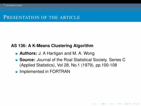
PRESENTATION OF THE ARTICLE
AS 136: A K-Means Clustering Algorithm
Authors: J. A Hartigan and M. A. WongSource: Journal of the Roal Statistical Society. Series C(Applied Statistics), Vol 28, No.1 (1979), pp.100-108Implemented in FORTRAN

INTRODUCTION
CLUSTERING
Clustering is the classical problem of dividing a data sample insome space into a collection of disjoint groups.
FIGURE : clustering

INTRODUCTION
THE AIM OF THE ALGORITHM
Divide M points in N dimensions into K clustersso that the within-cluster sum of squares is
minimized.
INTRODUCTION
EXAMPLE OF APPLICATION
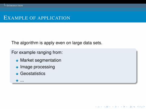
The algorithm is apply even on large data sets.
For example ranging from:
Market segmentationImage processingGeostatistics...

INTRODUCTION
EXAMPLE OF APPLICATION
MARKET SEGMENTATION
It is necessary to segment the Customer in order to know moreprecisely the needs and expectations of each group.
M: number of peopleN: number of criterion (age, sex, social status, etc ...)k: number of cluster
FIGURE : market segmentation
AGORITHM
1 INTRODUCTION
2 AGORITHM
3 DEMONSTRATION
4 CONVERGENCE AND TIME
5 CONSIDERABLE PROGRESS
6 THE LIMITS OF THE ALGORITHM
7 CONCLUSION

AGORITHM
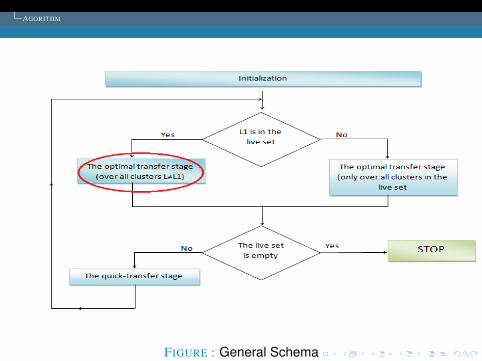
FIGURE : General Schema

AGORITHM
FIGURE : General Schema

AGORITHM
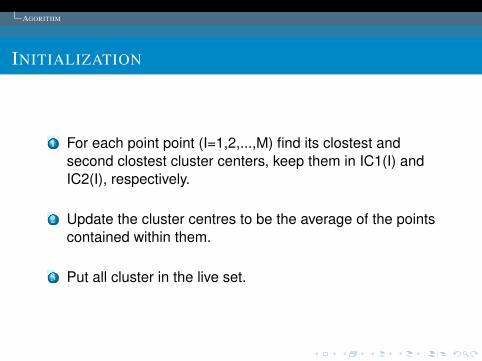
INITIALIZATION
1 For each point point (I=1,2,...,M) find its clostest andsecond clostest cluster centers, keep them in IC1(I) andIC2(I), respectively.
2 Update the cluster centres to be the average of the pointscontained within them.
3 Put all cluster in the live set.

AGORITHM
INITIALIZATION
1 For each point point (I=1,2,...,M) find its clostest andsecond clostest cluster centers, keep them in IC1(I) andIC2(I), respectively.
2 Update the cluster centres to be the average of the pointscontained within them.
3 Put all cluster in the live set.
AGORITHM
INITIALIZATION
1 For each point point (I=1,2,...,M) find its clostest andsecond clostest cluster centers, keep them in IC1(I) andIC2(I), respectively.
2 Update the cluster centres to be the average of the pointscontained within them.
3 Put all cluster in the live set.

AGORITHM
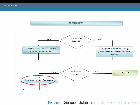
FIGURE : General Schema
AGORITHM
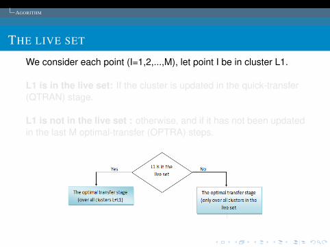
THE LIVE SET
We consider each point (I=1,2,...,M), let point I be in cluster L1.
L1 is in the live set: If the cluster is updated in the quick-transfer(QTRAN) stage.
L1 is not in the live set : otherwise, and if it has not been updatedin the last M optimal-transfer (OPTRA) steps.

AGORITHM
THE LIVE SET
We consider each point (I=1,2,...,M), let point I be in cluster L1.
L1 is in the live set: If the cluster is updated in the quick-transfer(QTRAN) stage.
L1 is not in the live set : otherwise, and if it has not been updatedin the last M optimal-transfer (OPTRA) steps.

AGORITHM
THE LIVE SET
We consider each point (I=1,2,...,M), let point I be in cluster L1.
L1 is in the live set: If the cluster is updated in the quick-transfer(QTRAN) stage.
L1 is not in the live set : otherwise, and if it has not been updatedin the last M optimal-transfer (OPTRA) steps.
AGORITHM
FIGURE : General Schema

AGORITHM
OPTIMAL-TRANSFER STAGE (OPTRA)
Compute the minimum of the quantity for all cluster L (L6=L1) ,
R2 =NC(L) ∗ D(I,L)2
NC(L) + 1(1)
NC(L): The number of points in cluster LD(I,L): The Euclidean distance between point I and cluster L
Let L2 be the cluster with the smallest R2

AGORITHM
OPTIMAL-TRANSFER STAGE (OPTRA)
If:NC(L1) ∗ D(I,L1)2
NC(L1) + 1≥ NC(L2) ∗ D(I,L2)2
NC(L2) + 1(2)
No reallocationL2 is the new IC2(I)
If:NC(L1) ∗ D(I,L1)2
NC(L1) + 1<
NC(L2) ∗ D(I,L2)2
NC(L2) + 1(3)
I is allocated to cluster L2L1 is the new IC2(I)Cluster centres are updated to be the means of pointsassigned to themThe two clusters that are involved in the transfer of point I atthis particular step are now in the live set

AGORITHM
FIGURE : General Schema

AGORITHM
FIGURE : General Schema

AGORITHM
FIGURE : General Schema
AGORITHM
FIGURE : General Schema
AGORITHM
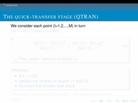
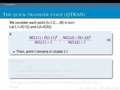
THE QUICK-TRANSFER STAGE (QTRAN)
We consider each point (I=1,2,...,M) in turnLet L1=IC1(I) and L2=IC2(I)
IfNC(L1) ∗ D(I,L1)2
NC(L1) + 1<
NC(L2) ∗ D(I,L2)2
NC(L2) + 1(4)
Then, point I remains in cluster L1
Otherwise,IC1↔ IC2Update the centres of cluster L1 and L2Its noted that transfer took place
This step is repeated until transfer take place in the last Msteps.

AGORITHM
THE QUICK-TRANSFER STAGE (QTRAN)
We consider each point (I=1,2,...,M) in turnLet L1=IC1(I) and L2=IC2(I)
IfNC(L1) ∗ D(I,L1)2
NC(L1) + 1<
NC(L2) ∗ D(I,L2)2
NC(L2) + 1(4)
Then, point I remains in cluster L1
Otherwise,IC1↔ IC2Update the centres of cluster L1 and L2Its noted that transfer took place
This step is repeated until transfer take place in the last Msteps.

AGORITHM
FIGURE : General Schema

DEMONSTRATION
1 INTRODUCTION
2 AGORITHM
3 DEMONSTRATION
4 CONVERGENCE AND TIME
5 CONSIDERABLE PROGRESS
6 THE LIMITS OF THE ALGORITHM
7 CONCLUSION

DEMONSTRATION

DEMONSTRATION
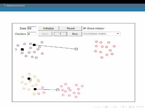
DEMONSTRATION
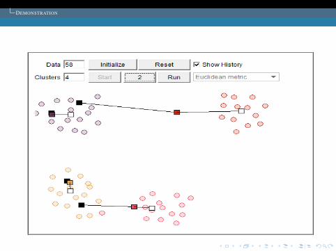
DEMONSTRATION
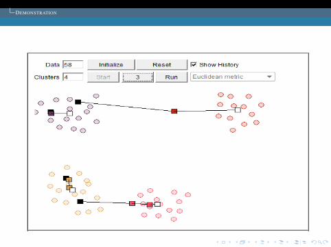
DEMONSTRATION

DEMONSTRATION

DEMONSTRATION

CONVERGENCE AND TIME
1 INTRODUCTION
2 AGORITHM
3 DEMONSTRATION
4 CONVERGENCE AND TIME
5 CONSIDERABLE PROGRESS
6 THE LIMITS OF THE ALGORITHM
7 CONCLUSION

CONVERGENCE AND TIME
CONVERGENCE
There are convergence, but the algorithm produces a clusteringwhich is only locally optimal!
FIGURE : A typical example of the k-means convergence to a localoptima
CONVERGENCE AND TIME
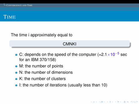
TIME
The time i approximately equal to
CMNKI
C: depends on the speed of the computer (=2.1×10⁻⁵ secfor an IBM 370/158)M: the number of pointsN: the number of dimensionsK: the number of clustersI: the number of iterations (usually less than 10)
CONSIDERABLE PROGRESS
1 INTRODUCTION
2 AGORITHM
3 DEMONSTRATION
4 CONVERGENCE AND TIME
5 CONSIDERABLE PROGRESS
6 THE LIMITS OF THE ALGORITHM
7 CONCLUSION

CONSIDERABLE PROGRESS
RELATED ALGORITHM
AS 113: A TRANSFER ALGORITHM FOR NON-HIERARCHIAL
CLASSIFICATION
(by Banfield and Bassil in 1977)
It uses swops as well as transfer to try to overcome theproblem of local optima.It is too expensive to use if the size of the data set issignificant.

CONSIDERABLE PROGRESS
RELATED ALGORITHM
AS 58: EUCLIDEAN CLUSTER ANALYSIS
(by Sparks in 1973)
It find a K-partition of the sample, with within-cluster sum ofsquares.Only the closest centre is used to check for possiblereallocation of the given point, it does not provide a locallyoptimal solution.A saving of about 50 per cent in time occurs in thek-Means algorithm due to using ”live” sets and due to usinga quick- transfer stage which reduces the number ofoptimal transfer iterations by a factor of 4.
THE LIMITS OF THE ALGORITHM
1 INTRODUCTION
2 AGORITHM
3 DEMONSTRATION
4 CONVERGENCE AND TIME
5 CONSIDERABLE PROGRESS
6 THE LIMITS OF THE ALGORITHM
7 CONCLUSION

THE LIMITS OF THE ALGORITHM
THE SELECTION OF THE INITIAL CLUSTER CENTRES
FIGURE : The choice of the initial cluster centres affect the final results

THE LIMITS OF THE ALGORITHM
THE SELECTION OF THE INITIAL CLUSTER CENTRES
THE SOLUTION TO THE PROBLEM
Proposed in the article:K sample points are chosen asthe initial cluster centres.The points are first ordered by their distances to the overallmean of the sample. Then, for cluster L (L = 1,2, ..., K), the1 + (L -1) * [M/K]th point is chosen to be its initial clustercentre (it is guaranteed that no cluster will be empty).
Commonly used:The cluster centers are chosenrandomly.The algorithm is run several time, then select the set ofcluster with minimum sum of the Squared Error.
THE LIMITS OF THE ALGORITHM
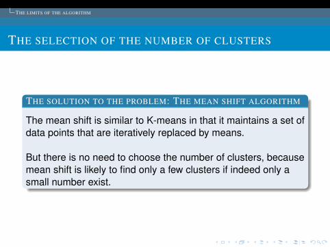
THE SELECTION OF THE NUMBER OF CLUSTERS
THE SOLUTION TO THE PROBLEM: THE MEAN SHIFT ALGORITHM
The mean shift is similar to K-means in that it maintains a set ofdata points that are iteratively replaced by means.
But there is no need to choose the number of clusters, becausemean shift is likely to find only a few clusters if indeed only asmall number exist.
THE LIMITS OF THE ALGORITHM
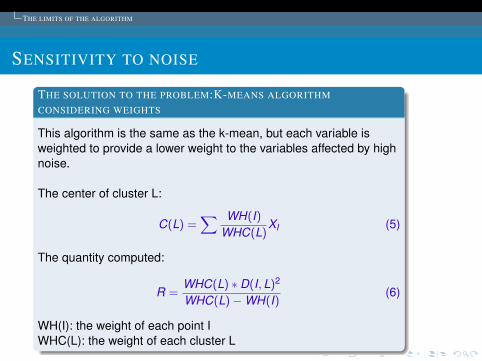
SENSITIVITY TO NOISE
THE SOLUTION TO THE PROBLEM:K-MEANS ALGORITHM
CONSIDERING WEIGHTS
This algorithm is the same as the k-mean, but each variable isweighted to provide a lower weight to the variables affected by highnoise.
The center of cluster L:
C(L) =∑ WH(I)
WHC(L)XI (5)
The quantity computed:
R =WHC(L) ∗ D(I,L)2
WHC(L)−WH(I)(6)
WH(I): the weight of each point IWHC(L): the weight of each cluster L
CONCLUSION
1 INTRODUCTION
2 AGORITHM
3 DEMONSTRATION
4 CONVERGENCE AND TIME
5 CONSIDERABLE PROGRESS
6 THE LIMITS OF THE ALGORITHM
7 CONCLUSION

CONCLUSION
CONCLUSION
This algorithm has been a real revolution for the clusteringmethods:It produces good results and a high speed ofconvergence.
This algorithm possesses flaws, but many algorithmsimplemented today are arising from it.

CONCLUSION
REFERENCES
J. A. Hartigan and M. A.Wong (1979) Algorithm AS 136: AK-Means Clustering Algorithm. Appl.Statist., 28, 100-108.
http://home.dei.polimi.it/matteucc/Clustering/tutorial_html/AppletKM.html
http://en.wikipedia.org/wiki/K-means_clustering

Thank you for your attention !!!Retour.