HYPOTHESIS TESTING FOR DIFFERENCES

BETWEEN MEANS AND BETWEEN PROPORTIONS

ASSUMPTIONS

Selecting an appropriate test for analysing hypotheses of difference depends on a number of important assumptions particularly relating to parametric and non-parametric assumptions

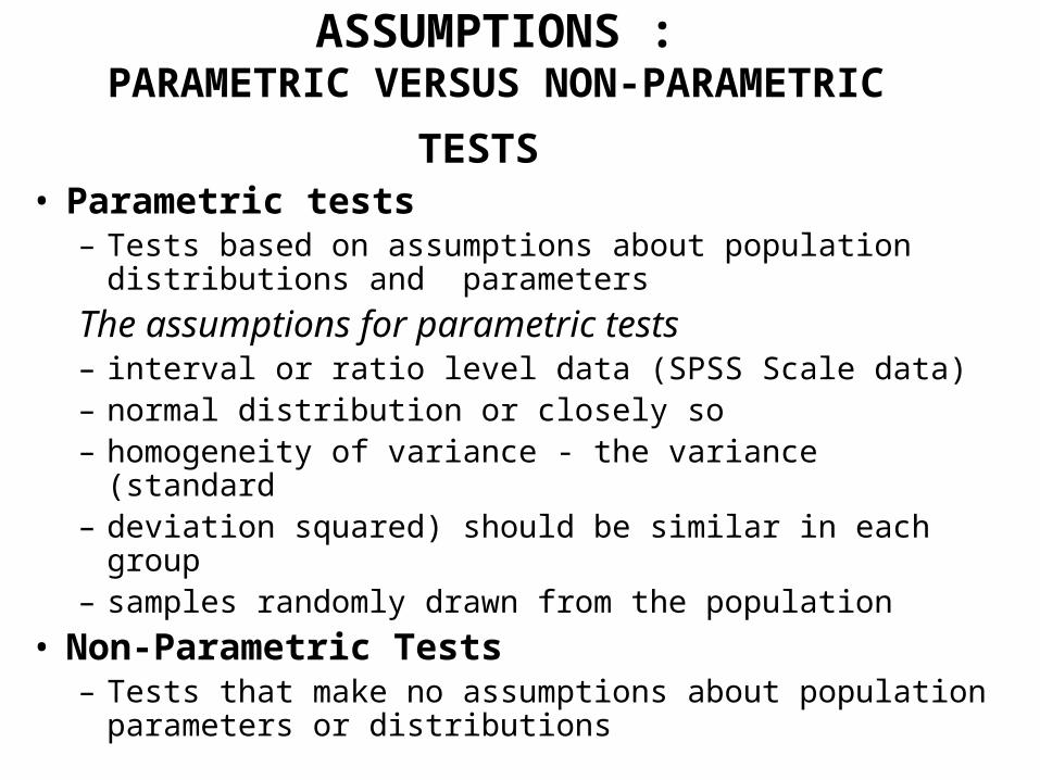
ASSUMPTIONS :PARAMETRIC VERSUS NON-PARAMETRIC

TESTS • Parametric tests

– Tests based on assumptions about population distributions and parameters

The assumptions for parametric tests– interval or ratio level data (SPSS Scale data) – normal distribution or closely so– homogeneity of variance - the variance (standard – deviation squared) should be similar in each group– samples randomly drawn from the population

• Non-Parametric Tests – Tests that make no assumptions about population

parameters or distributions

DesignsHypotheses of differences can involve different research

designs

• Independent Groups or Between Groups Design – Two independent samples are selected randomly and compared

often in a control versus experimental contrast.• Repeated Measures Design

– One sample is measured in both conditions – a before and after approach.

• Paired or Matched Samples Design– Individuals, units or observations are matched as pairs on one or

more variables and allocated at random one to each sample.

Different forms of the t test and ANOVA exist for these designs

t -TEST t Tests are parametric tests and assume

• normal distribution or approximately so, • random selection of sample elements, • homogeneity of variance or approximately

so and • scale data measurement.

Types of t TestThree main types of t test exist:

1. The one sample t test

2. The independent group t test between two separate random samples

3. The repeated (or paired) measures t test between two testings of the same sample or between two paired samples

THE ONE SAMPLE t TEST : TESTING HYPOTHESES FOR SINGLE SAMPLES

t = sample mean – population mean estimated standard error of mean

(derived from sample)

(notice similarity to Z. t = Z when sample size is large)

– tests the null hypothesis that the mean of a particular sample differs from the mean of the population only by chance

1. Enter data as a single variable (here as “runs”)

2. Analyze > Compare Means > One-Sample t-test (normally we use more than 5 scores)

One Sample T testExample from SPSS

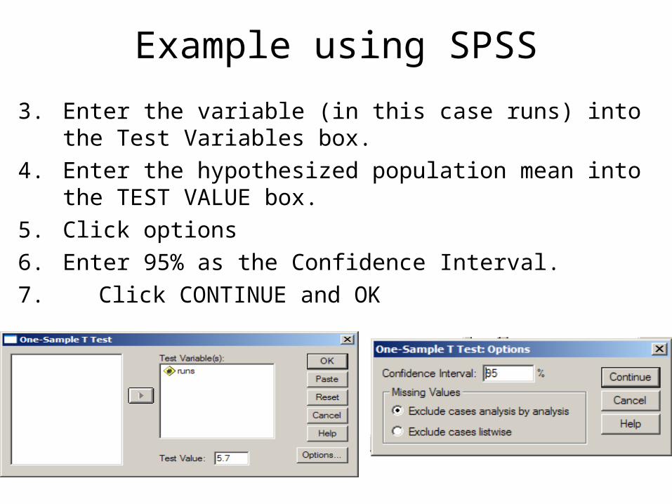
3. Enter the variable (in this case runs) into the Test Variables box.

4. Enter the hypothesized population mean into the TEST VALUE box.

5. Click options6. Enter 95% as the Confidence Interval.7. Click CONTINUE and OK

Example using SPSS

8. The calculated probability (Sig. (2-tailed)) is .257 which is greater than .05 – So the result is not significant.

t = 1.319, p = .257 so your mean of 7.4 could have come from a distribution with a population mean of 5.7

One-Sample Statistics

5 7.40 2.881 1.288RUNSN Mean Std. Deviation

Std. ErrorMean

One-Sample Test

1.319 4 .257 1.70 -1.88 5.28RUNSt df Sig. (2-tailed)

MeanDifference Lower Upper

95% ConfidenceInterval of the

Difference

Test Value = 5.7

Example using SPSS

More frequently we want to compare two sample means.

There are two types of such comparisons.1. Where we have two means which are calculated from

two different samples (the populations are independent). e.g. if we wanted to compare attitudes of males with those of females towards some issue and determine whether one gender was more positive than the other a two-sample t-test may be used here.

2. Where we have two means which are calculated from the same sample when we have measured the variable at two different times. E.g. Change in attitude of the whole group over time, a Repeated Measures (Paired Difference) t-test may be used.

Comparing Means With t Tests

Independent Groups t Test. Between Groups Design

• The Independent Groups t test is used to determine whether two random samples are likely to come from the same population.

• If there is a statistically significant difference between them then the null hypothesis that their sample means are simply two chance variations around a population mean is rejected.

• Often used in the experimental versus control group set-up – the Between Subjects design.

ASSUMPTIONS FOR INDEPENDENT GROUPS t TEST

– measurements are on interval scale– subjects are randomly selected from a defined

population– the variances of the scores for the two

samples or occasions should be approximately equal (homogeneity)

– the population from which the samples have been drawn is normally distributed.

• Suppose we want to compare two parallel classes of students studying Tax Law. At the beginning of the year, students were randomly assigned to each class.

• Each class is taught using a different method; one by

usual face-to face teaching ; the other by individual study using a computerized module presentation.

• After 6 months, we test whether performance (on a test with a maximum value of 20) varies between the two classes (two-tailed non-directional test).

• For alpha = .05

Example of Independent t test

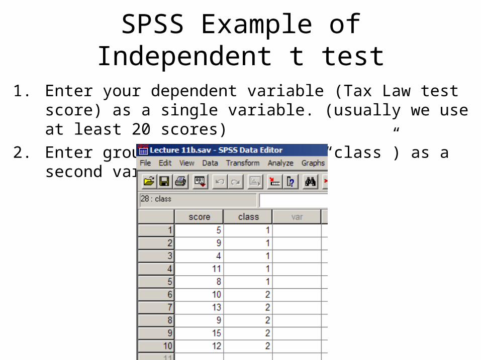
1. Enter your dependent variable (Tax Law test score) as a single variable. (usually we use at least 20 scores)

2. Enter group membership (here “class”) as a second variable.

SPSS Example of Independent t test

3. Analyze > Compare Means > Independent-Samples t-test

4. Enter your dependent variable (“score”) in the TEST VARIABLES box, and your grouping variable (“class”) in the GROUPING VARIABLE box.

5. Click DEFINE GROUPS

SPSS Example of Independent t test

5. Enter the codes you used to define your two groups (here “1” and “2”).

6. Click Continue7. Click OK

SPSS Example of Independent t test

8. Interpret: The mean for Class1 = 7.40, for Class2 = 11.80, d.f. = 8, t8 = -2.63. The calculated probability for such a mean difference = .030, which is less than the alpha of .05, and so is significant.

9. So we conclude that the performance of the two classes is significantly different, t8 = -2.63, p < .05, with class two doing significantly better.Group Statistics

5 7.40 2.881 1.2885 11.80 2.387 1.068

CLASS12

SCOREN Mean Std. Deviation

Std. ErrorMean

Independent Samples Test

.379 .555 -2.630 8 .030 -4.40 1.673 -8.259 -.541

-2.630 7.733 .031 -4.40 1.673 -8.282 -.518

Equal variancesassumedEqual variancesnot assumed

SCOREF Sig.

Levene's Test forEquality of Variances

t df Sig. (2-tailed)Mean

DifferenceStd. ErrorDifference Lower Upper

95% ConfidenceInterval of the

Difference

t-test for Equality of Means

SPSS Example of Independent t test

Levine’s test suggests homo-geneity of variance assumption OK

p <.05

Mean difference being tested

DEGREES OF FREEDOM

• Abbreviated to df • The number of values free to vary in a set

of values • Used to evaluate the obtained statistical

value rather then N • df usually = N – 1 per sample (group)

Repeated Measures or Matched Pairs Design (Parametric test)

• Assumptions of the Test– measurements are on interval scale– subjects are randomly selected from a defined

population– the variances of the scores for the two

samples or occasions should be approximately equal

– the population from which the samples have been drawn is normally distributed.

Suppose we want to compare the effects of a training course on performance at two points in time. (a) prior to start of course, and (b) at end of course. Use a two-tailed test at alpha = .05

• Enter the data for performance at the beginning of the year as a variable (“before”).

• Enter the data for performance at the end of the year as a variable (“after”). (We would normally use at least 20 pairs of scores)

Repeated Measures or Paired Samples SPSS Example

3. Analyze > Compare Means > Paired-Samples t-test4. Select both variables (“before” and “after” and

enter into PAIRED VARIABLES box)5. Click Options.

Repeated Measures or Paired Samples SPSS example.

Repeated Measures or Paired Samples SPSS example.

6. Select 95% as your confidence interval.7. Click Continue.8. Click OK

9. The mean for Before = 8.40, After = 11.80, d.f. = 4,

t4 = -13.880, the calculated probability is .000, which is less than the alpha level of .05 – and so is significant.

10. So we conclude that the performance of the class has significantly changed from before-training to after-training, t4 = -13.88, p < .001.

Paired Samples Statistics

8.40 5 2.881 1.28811.80 5 2.387 1.068

BEFOREAFTER

Pair1

Mean N Std. DeviationStd. Error

Mean

Paired Samples Test

-3.40 .548 .245 -4.08 -2.72 -13.880 4 .000BEFORE - AFTERPair 1Mean Std. Deviation

Std. ErrorMean Lower Upper

95% ConfidenceInterval of the

Difference

Paired Differences

t df Sig. (2-tailed)

Repeated Measures or Paired Samples SPSS example.

We compare this mean difference

p is highly significant