SLAC-PUB-4680 August 1988

(T)

CONFORMAL BRANCHING RULES AND MODULAR INVARIANTS

MARK A. WALTON*

Stanford Linear Accelerator Center

Stanford University, Stanford, California 94309, USA

ABSTRACT

Using the outer automorphisms of the affine algebra S-U(n), we show

how the branching rules for the conformal subalgebra SU(pq) I

@J(P) x s%) may be simply calculated. Modular-invariant com-

binations of SU( ) h n c aracters are obtained from the branching rules.

Submitted to Nuclear Physics B [FS]

-

* The author’s research was supported by a postdoctoral fellowship from NSERC of Canada, and by the U.S. Department of Energy under contract DE-AC03- 76SF00515.

- 0. Introduction

Two-dimensional conformal field theories describe critical points of second

order phase transitions and classical vacua of strings. Consequently, the classifi-

cation of such conformal field theories is an important open problem.

A tractable subclass is the set of rational conformal field theories [l]. In-

cluded are the Wess-Zumino-Witten (WZW) models [2], conformal field theories

constructed from them by the coset construction [3], and orbifolds of them (see,

for example refs. [4] and [5]). WZW models are of central importance in the

study of rational conformal field theories.

The symmetry algebras of WZW models are of the affine KaE-Moody type

(for reviews, see refs. [6] and [7]). Th ese algebras and their representations are

the subject of this paper.

We will show that the branching rules for the affine subalgebra

can be easily obtained from some simple branching rules for the finite Lie subal-

gebra

sub?) 1 SU(P) x SW - (0.2)

As far as we know, the branching rules for (0.1) have not been calculated previ-

ously.

- Modular invariance is a powerful restriction on the spectra of conformal field

theories. Besides being intrinsically interesting, the branching rules for (0.1) allow

2

the construction of various modular-invariant combinations of E%(n) characters

in a simple way. The modular invariants are possible partition functions for

systems with S^u( n s ) y mmetry.. The classification of such modular invariants has

only been carried out for the S%(2) case [8]. Our results aid in generalizing that

classification.

The format of this paper is as follows: in the second section we review affine

KaE-Moody algebras mainly to establish notation; the third section describes the

method of calculation of the branching rules, the fourth illustrates the method

with two examples, and the final section is a short conclusion.

1. Review and Notation

Let 6 denote the affine Ka&Moody algebra that is the central extension of

the loop algebra of the finite-dimensional Lie algebra jj* The algebra fi is

[J;, J;] = fabc J&+n + k~ab6,+,,o . (1-l)

We will sometimes include the value of k E 2 by writing fi = 6”. Setting the

integral indices m and n in (1.1) to zero reduces this algebra to the finite one

g c &

The Sugawara construction

1 ‘, = 2(k + h”) nEZ c

44 Kab : Jk+n Jb, : -6”“~ 3 (14

* In general we use the-convention that carets denote objects associated with affine algebras and bars their finite algebra counterparts.

3

associates with 6 the Virasoro algebra -

[j&L,] = (m - n)Lm+n + g (m - l)m(rm + 1) &a+n,o , (l-3)

with central charge

k - dimij ‘(g) = k + h” ’ (1.4

Here Kab, h” are the Killing form and dual Coxeter number of 8, and the normal

ordering is defined in the usual way.

The Cartan subalgebra k of 6 contains the Cartan subalgebra 6 of 0, with

elements hi(i = 1,. . . , r) plus the extra element ho. We denote the elements of

i by hp(p = O,l,..., r). Dual to these elements, living in the weight space k*,

are the fundamental weights UP:

wc”(h,) = 6; . (1.5)

Associated with each h, is a co-root ai, also living in the weight space i*, so

that we have

The dot product is determined from the Cartan matrix A by the definition of its

elements:

where a root c+ and its co-root LYE are multiples of each other:

There is an extra- operator which commutes with the h,; it is Lo of (1.2).

4

The Cartan subalgebra can be extended to ie having elements h, and d = -Lo.

We denote the weight dual to d by 6

6(d) = 6(-Lo) = 1 , (1.8)

and the co-root corresponding to d by Ao

6 -A0 = 6(d) = 1 . (1.9)

With the usual conventions

Ao(hi) = S;, i = 1,. . . ,I- ,

no(d) = A, (-Lo) = A0 .A0 = 0 ,

the scalar product on the extended weight space i*e is Minkowskian. Let

(1.10)

be the highest root of 8. The kp, k”p are known as marks and co-marks, respec-

tively with Cc0 z kov E 1. Then if B, C E i*,, we write

B = &wp + psS = (&w” = B, k[B], ps)

C = rpwp + 7~6 = (7iw’ = c, k[C],7s) (1.11)

where k[B], k[C] are the levels of B and C, respectively,

k[B] = &k”j‘ k[C] = rpkvp . (1.12)

Then the dot product on the expanded weight space i*e takes the form

-

II- c = B-c + k[B]rs + ,&k[C] . (1.13)

5

With the above notation, the simple roots and fundamental weights of ij can

be written

ai = @,o,o) cl0 = (-$,O,l)

wi = (ai, k”‘,O) w” = (0, 1,0) .

So the Dynkin diagram of 6 is the extended Dynkin diagram of jj. The

Dynkin diagram of Sb(r + 1) is shown in Fig. 1. Outer automorphisms of 6

are manifested as automorphisms of the Dynkin diagram of 8. From Fig. 1 we

see that S^U(r + 1) h as such an automorphism generated by Awp = wp+l. Note

that this is not an automorphism of the extended algebra. Specifically, it doesn’t

commute with d = -LO. Since LO is physically an energy operator, the usefulness

of this automorphism is not obvious, but non-zero as we will see.

Of physical interest are the highest weight representations of i. They are

generated from a “vacuum” state IM >, labeled by a dominant weight

M = +&w’” = (li& Mpkvr,O) . (1.14)

The “vacuum” satisfies

JilM>=O, n>O

J,alM>=T&iM> 9

where Tz are the matrices representing the generators of g in the finite di-

mensional representation labeled by I@. We will use the notation M =

[MoMI.. . M,.] E [M] to d enote the weight M and corresponding highest

-weight representation. Similarly, representations of g will be denoted by i@ =

(MlM2... M,.) = (M). For unitary highest weight representations [M] of (l.l),

6

we must require -

k[M] = MpkVp = k . (1.15)

The states in [M] having a fixed eigenvalue of Lo fall into a finite sum of

irreducible representations of g. For example, the lowest value of Lo is

Lo = h[M] - $) = Aa - (M + 2p) c(g) 2(k+h”) - 24 ’

(1.16)

where B is the half-sum of positive roots of g. The states of [M] with this value

of LO fill out the representation l@ = (M).

The character of a highest weight representation M = [M] is defined by

ch&T,z) = tr[M]e Sni(TLo+dL) . (1.17)

. The characters at z = 0

x[M] = x[MoMl,... Mr] = ch&,O) 7 (1.18)

are Virasoro characters, since they involve only LO. The x appear in the partition

function

Z(7) = tr e 27ri(T&-r&J)

= c ZMN x[M]x[Nl* - WISNI

(1.19)

For a physically sensible partition function, .Z’MN E Z+, and for [M] =

[10...0],2~~ = 1. It is a nontrivial and in general unsolved problem to de-

Xermine all possible modular-invariant matrices 2 for a given group g and level

k.

7

., :

The modular transformation properties of the characters was found in Ref. [9].

Transforming by S : r + -l/r reveals the asymptotic behavior of the characters:

as7-+ 0, x[M] - e[M]e2"'c(g)/24'. (1.20)

The .!![M] can be calculated entirely from objects relevant to the finite algebra g :

t[M] = ; I I

l/2 [k[M] + h”]-’ -j-J 2 sin I(k~M~~)~vM] -

[- (1.21)

WA+

Here A+ denotes the set of positive roots, M = (Ml . . -M,.), and -li;, & are,

respectively, the weight and root lattices of g.

Knowledge of affine subalgebras of affine algebras is nowhere near as extensive

as that of finite subalgebras of finite algebras. However, each finite subalgebra

3’ of a finite algebra g induces an affine subalgebra 3 of 6 (see, for example,

Ref. [lo]). 0 ne identifying feature of a finite subalgebra 3 c g is the index of

embedding 0, equal to the ratio of the length squared of the highest root of g

to that of 3 embedded in g. The affine subalgebra induced by 3“ C g (obvious

notation) is juk C 8”.

All other information concerning a finite subalgebra 3” c g is contained in

the so-called projection matrix F [ll]. F is a (rank 3 = r”) x (rank g = r)

matrix relating weights of g to the weights of 3 onto which they are projected. If

(M) = (MlM2-M,) is a weight of g, it is projected onto the weight (M)FT.

We can define an affine projection matrix $, containing F, so that an affine

-weight [M] = [MOM1 -- . M,] is projected onto the weight [M]PT. For our pur-

poses, we can assume- that ? is semi-simple, with f simple terms, 3 = c{=,j;,

8

the terms having embedding indices-ai.- Then @ will be a (r”+ f) x (r + 1) matrix.

The extra column is determined by the projection of the weight [loo. . -01 = w” of

el. Clearly, w” is projected onto Cif=, cr;wr;,, where w?~, is the 0-th fundamental

weight of $. The extra rows are easily determined by the values a;.

A special class of affine subalgebras is induced by 3” c ZJ when c(j) = c(g).

These are the so-called conformal subalgebras and we denote them by juk a ek.

Now this situation is only possible for k = 1 [12], so without loss of generality,

we write j” 4 ij’.

The name conformal subalgebra is appropriate because the Sugawara stress

tensors of j” and G1 are equivalent [3,7]. H ence the Virasoro characters ch(T, z =

0) of ij are finitely reducible in terms of the Virasoro characters of 3, and the

relation extends to the full characters ch(T, z # 0). C onversely, finite reducibility

. -is possible only if the central charge of the embedded algebra equals that of the

larger algebra.

Complete lists of conformal subalgebras have been compiled [12], and they

include

sb(pq) D k(p)’ X s^u(q)p (1.22)

In the next section, we show that the branching rules for this conformal subal-

gebra can be easily computed from the well-known branching rules for the finite

algebra counterparts SU(pq) > SU(p) x SU(q).

9

2. Calculation of the Branching Rules

Consider a conformal subalgebra 3” a 3’. Suppose [M] is a highest weight

representation of 8 satisfying k[M] = 1, i.e., it is a basic highest weight represen-

tation of 4. Then the branching rule for [M] takes the form

WI + c Nm Iml P-1) k[m]=k

where N,cZ+ and the sum is a finite one, over all highest weight representations

of 3” satisfying k[m] = k. Furthermore, there is a branching rule for each level

one representation of i.

.

Since the Sugawara stress tensors for 3’ and 3” are equivalent, so are their

lowest moments LO. Each state in [M] must be represented by a state in one of

the [m] for which N, # 0, and having the same eigenvalue of LO. Every state

-in [$I has Lo-eigenvalue equal to h[M] - c/24 of (1.16) mod an integer; and

similarly for [ml. Therefore every [m] for which N, # 0 in (2.1) must satisfy the

level-matching condition [9]:

0 5 h[m] - h[M] c 2 . (2.2)

Clearly, (2.1) implies

x[M] = C NmX[mI .

k[m]=k

By (1.20), as r + 0, this yields the asymptotic constraint

P-3)

- l[M] = c N,l[m] .

k[m]=k (2.4

For many conformal subalgebras, asymptotics and level-matching are sufficient

10

to determine the positive integers Nrn- and therefore the branching rules (2.1)

[ 13,141. But this is not true for (1.22).

Let VB,Vb,Vp denote vectors in SU(pq), SU(p) and SU(q), respectively.

Then the subgroup SU(p)x SU(q) c SU(pq) is defined by the branching rule

p = VbVP (2.5)

The projection matrix for the corresponding affine subalgebra can be taken to be

j-i%

Q q-1 q-1 0 1 0 . . .

0 0 1 s . *. . .

0 0 0 . . .

- - -

P P-1 P-2 0 1 2 . . .

0 0 0

0 0 0 . .

q-l q q-l q-l 0 0 1 0 . . .

0 0 0 1 . . -. . .

1 0 0 0 . . .

- - - -

1 0 0 0

p-l p p-1 p-2 *..

0 0 1 2

0 0 0 0 . . .

(2.6)

or a similar matrix, with the roles of SU(p) and SU(q) interchanged.

Now consider the outer automorphism group of S?J(pq), generated by Ad‘ =

wp+l (here w p = wV if p = Y mod pq). Clearly, (2.6) reveals there is an image of

AP in the outer automorphism group of E%(p) x E%(q). If we let a and CY be the

outer-automorphism-generators for S*U(p) and f&(q), respectively, then we have -

AP=a . (2.7)

11

Reversing the roles of p and q-in (2.6) yields

Aq=a . (2.8)

If we let these relations act on the pq branching rules of (1.22), we can group

them into either p sets of q each that are related by (2.7), or q sets of p each that

are related by (2.8).

Suppose we have p sets each containing q related branching rules. We can

obtain an entire branching rule, and therefore all q of them, by computing pieces

of each of the q branching rules. There are pieces of each of these branching rules

that can be computed simply from finite Lie group theory. The states with lowest

eigenvalue of LO in the level one representations of SU(pq) are the scalar and basic

representations of SU(pq). Th e b ranching rules of the latter into representations

of SU(P)X SW are easily computed and that for the former is trivial. These

can then be translated into part of the appropriate affine branching rule. We

repeat this procedure for all q branching rules and use (2.7). The sole remaining

question is do we obtain the full branching rule? The answer is yes, as can be

verified by the sum rule of (2.4). R emarkably, a few simple finite branching rules

suffice to determine the affine ones.

The finite branching rules are easily computed using Young tableaux. The

.&th basic representations ae of SU(pq) can be represented by a tensor with

e antisymmetrized indices and therefore by a Young tableau with .f? boxes for

--SU(p) and also one of .f! boxes for SU(q). The SU(p) and SU(q) Young tableaux

must be paired to respect the antisymmetry of the original tensor.

12

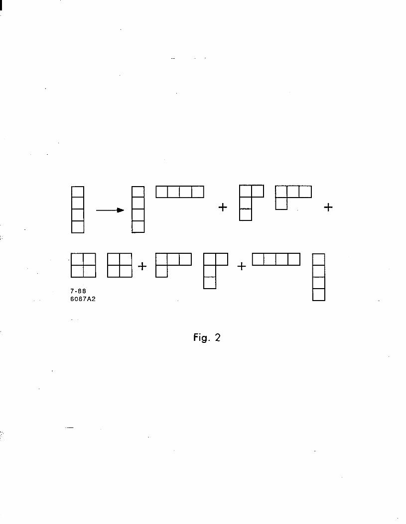
As an example, consider-the branching of the fourth basic representation

ti4 of SU(pq), illustrated in Fig. 2. Note that all Young tableaux made of four

boxes are involved, and the SU.(q) Y oung tableaux are obtained. from their SU(p)

partners by interchanging rows and columns. Furthermore, Fig. 2 gives the a4

branching rule for all p and q.

The computation would be even simpler if A itself had an image in the outer

automorphism groups of S?J(p) and f&(q). If this were true, we could write

A = aUcxV (2.9)

for some u, v. However, if p is a multiple of q, (or vice-versa) then ANq =

AP (A Np = AQ) for some N. Equations (2.7) and (2.8) then yield uN = cz(aN =

a) which is impossible.

We can, however, express A as in (2.9) when p or q is not a multiple of the

other. By substituting (2.9) into (2.7) and (2.8), we obtain

pv = 1 mod q (2.10)

qu = 1 mod p.

These equations are sufficient to determine the integers u and v. Therefore, when

p is not a multiple of q and q is not a multiple of p, we can write the conformal

branching rules by writing that of one basic representation, since (2.9) acting on

it determines the rest.

In the following section we present two examples; one for which q is a multiple

--of p so that we use the image of AP, and one for which p and q are not multiples

of each other, so that we can use the relation (2.9).

13

- 3. -Examples

The first example we consider is the conformal subalgebra

S-U(18) D S-U(3)6 x S-U(6)3 , (3.1)

i.e., the general case (1.22) with p = 3 and q = 6. Since q is a multiple of p,

the generator A of the outer-automorphism group of SU(18) has no image in the

outer-automorphism group of k(3) x &J(6), but A3 does.

Equation (2.7); A3 = CX, relates the branching rules for the representa-

tions w”,w3,w6,wg,w12,w15. The highest weights for the lowest Lo-eigenvalue

-3 -6 -9 -12 -15 subspaces of these representations are 0, w , w , w , w , w , respectively. The

branching rules for these finite Lie representations may be obtained by the Young

tableau method exemplified in Fig. 2. the two “longest” are:

LP + (oo-03000)+(11-11100)+(30-20010)+

(60 -00000)+(41-lOOOl)+ (03 -00200)+

(22-01010)

a9 -+ (oo-00300)+(11-01110)+(30-02001)+

(41-11000)+ (03 -10020)+

(14 -00011)+(33 - 00100)+

(22 - 10101).

(3.2)

-A third, that for a12, is determined from that of @ by replacing SU(3) and

SU(6) representations by their contragredient representations.

14

These three finite branching rules provide parts of the affine branching rule

we want:

w6 + [600- 0030dO]+[411- 011100]+[330 -020010]+

[060 - 300000]+ [141-110001]+[303 - 100200]+

[222 -101010]+ .*.

wg + [600-000300]+[411- 001110]+[330 -002001]+

[141- 111000]+[303 -010020]+

[114 -100011]+[033 - 200100]+ (3.3)

[222 - 010101]+ **.

w12 + [600-000030]+[411-000111]+[330- 100200]+

[303 -001002]+

[006 - 300000]+[114 -llOOOl]+

[222 - 101010]+ *.*.

With A3 = CY, applying Ae6,ilmg, and A-12, respectively, to these branching

rules yields the branching rule for w”:

w" + [600 - 300000]+[411- 110001]+[330 -001002]+

[060 -000030]+[141-000111]+[303 - 020010]+ (3.4

[006 -003000]+[114-011100]+[033 -100200]+

[222-101010].

-

15

The branching rules for w’ and w2 can be derived similarly:

wl-+[402 -020001]+[510-210000]+[213-OllOlO]+

[240-OOOlOi]+[O51-000021]+[321- lOlOOl]+

[024 -010200]+[105 -002100]+[132-lOOllO] P-5)

w2 -+[420 - 201000]+[501-120000]+[231- lOOlOl]+

[042 -100020]+[150-000012]+[123-OlOllO]+

[204 -002010]+[015 -001200]+[312-OllOOl].

That these branching rules are complete can be verified using the asymptotic

sum rule (2.4). Equations (3.4) and (3.5) together with A3 = CY determine the

branching rules for all level one representations of Sb(18).

We now consider an example for which there is an image of A in the outer-

automorphism group of the subalgebra. For the case

Sti(12) D S*u(3)4 X Sti(4)3

solving (2.8) and (2.7) gives

A = act3.

The branching rule for the finite representation a5 is easily found to be

a5 + (31-100)+(12-011)+(20- 201)+(01-120)

which implies for the affine case

L. w5 --i [031 - 2100]+ [112 - 1011]+ [220 - 0201]+ [301- 01201 + a*.

P-6)

(3-7)

(3.8)

(3-g)

16

Acting on (3.9) with Ae5 s aa! does not yield the full branching rule. The

complete result is

w" -+[400 - 3000]+[031- 2100]+[112 -loll]+ (3.10)

[220 -0201]+[301-01201.

. The first term in (3.10) is obvious, although it cannot be obtained from (3.9).

As in the previous example, that nothing is missing can be verified using the

asymptotic sum rule.

4. Modular Invariants

.

As an application of our results we will derive some modular-invariant com-

,-binations of various S?J(n) characters of the form (1.19). For every affine algebra

ik there exists a trivial “diagonal” modular-invariant Zd given by replacing ZMN

with ~MN in (1.19).

If 3 has a conformal subalgebra fi D f, then a non-trivial modular-invariant for

f^ may be obtained by simply substituting the branching rules for the subalgebra

in character form [15]. If, furthermore, f^ = 3 + I, we can obtain a modular

invariant for 3 by projecting onto the E-singlet part of Zd [13]. That is, if after

substituting the branching rules for b D 3 + f into .Zd we keep only those terms

proportional to XcxL, where C is the iE representation contragredient to a, the

result is a modular-invariant combination of 3 characters.

- We now apply this procedure to our conformal subalgebra, equation (1.22).

First consider the case p = 2. Using the methods described above, we can find

17

the branching rules in closed form. For q odd we have

Q we --+ c aed(qT1)12[(q - T)~O + rwl, wr/2 + wq--‘/2]

r=0 re2z

(q E 22 + 1).

(4.1)

Here the wj‘ are the fundamental weights of the SU(n) groups involved (i.e.,

n = 2q, 2, or q) and a and o. are the outer-automorphism generators of E%(2)

and k(q), respectively. For q even we obtain

w2e + 2 ae[rWo + (q - r)w1,w(Q--‘)/2 + W(q+r)/2] r=O

rc2Z

(cl E 22)

(4.2)

and

w2t+1 + 2 1

a! rw” + (q - l)wl,w(q-r+l)/2 + w(q+r+l)/2]

r=1 re2z+1 (4.3)

If we substitute these results into the diagonal S’b(2q) modular invariant and

then project onto the SU(q) -singlet part as described above we obtain SU(2)

modular-invariants. In fact, for q odd we get the trivial diagonal invariants. But

for q even we obtain the partition functions for strings on the group manifold

SO(g) E SU(2)/&, first derived in [5].

18

Repeating the procedure-for p = 3 yields the following modular-invariants:

for k $ 32 we get

2 = c 2 IAr[abb]12 a#br=O

+ C 2 Ar[d~](ArR[thi~])* + C.C. a#b#c#a r=O

b+lc=k mod 3

where

A[&] = [cab] lqabc] = [cba] P-5)

For k = 3t the modular invariants are

2 = c 12 A’[abb],” + 31[ttt]12 afb r=O

+ 2 2 Ar+s[&] (AVW [&]) * + C.C. \

a#b#c#a r=O e=O b+Sc=k mod 3 J

(44

(4.6)

Equations (4.4) and (4.6) can ‘be used to complete a possibly exhaustive list of

SU(3) modular-invariants [16].

The first few in these series agree with the partition functions for strings on

the group manifold SU(3)/& found in [5]. So (4.4) and (4.6) probably constitute

the full infinite series of such partition functions. Since it seems to hold for

p = 2 and 3, we conjecture that the partition functions for strings on the group

manifolds SU(p) /Zp can be calculated in the same manner.

- We must mention that SU(p)/Zp partition functions and many more modular-

invariants were found- previously by Bernard [ 171. It is not surprising that our

19

results agree with his since the main tools in his work, as in ours, were the outer-

automorphisms of affine Lie algebras. However, Bernard did not work out the

branching rules for (1.22) as we did, and these contain much more information

than just the partition functions he derived. As a simple illustration of this, we

will work out another modular-invariant from a branching rule used above to

. obtain an SO(3) partition function.

It is possible to generalize the procedure for obtaining modular-invariants

from 3 D j + i in the following way [18]. Suppose after substituting the branching

rules into the diagonal invariant for 3 we obtain the modular-invariant:

C z,m,,nX[~]X[mlX*[ulX* bl 9 (4.7)

-where [I-J], [VI, d enote 3 representations and [ml, [n] denote i representations.

Equivalently, we can say that Zpm,vn is a modular-invariant tensor. But we can

obtain another such tensor by contraction with an invariant tensor given by a i

modular-invariant:

The procedure we have used above is just a special choice of the tensors 2 and

If we use the branching rules for

S^u(20) D &(2)l” X siJ(lo)2

20

(4.9)

in the trivial invariant of SU(20). and contract with the exceptional k(2)

modular-invariant [8]

Z(E6) = ,[lO,O] + [46]l” + ][73] + [37]]” + ][64] + [O,1o],2 (4.10)

we obtain a new SAU(10)2 modular-invariant:

4 / Z=C

e=o I [2wl] + [w3+e + w7+e1 2+

[ w2+e + ,s+e] + Iw4+e + ,7+e]

2

[ wl+e + w*+e] + [2w5+e

’ I

.

2

+ (4.11)

We also mention that there are uses for conformal branching rules other than

the -derivation of modular-invariants. For example, in ref. [ 191 it was shown how

they can provide information about certain conformal field theories defined by

the GKO coset construction [3].

5. Conclusion

In summary, we have shown how to use the outer-automorphism group of

Sk(n) to calculate branching rules for the conformal subalgebra S?J(pq) D S^u(p) x

SU(q), given the branching rules for the basic representations of SU(pq) in the

subalgebra SU(pq) > SU(p)x SU(q).

- We have also constructed modular-invariant combinations of SU(n) charac-

ters from our results. We found explicitly the partition functions for strings

21

on the group manifold SU(n-) /Zn f or n = 2 and 3, and showed how the re- -

sults may be obtained for arbitrary n. Generically, our branching rules yield

modular-invariants of the type found previously by Bernard [17], who also used

the outer-automorphism group. However, other modular-invariants can also be

obtained, as we illustrated.

The method used here may be extended to other conformal subalgebras

[20], and possibly also to nonconformal affine subalgebras. We believe that our

method, in conjunction with previously known ones, should make possible the

calculation of the branching rules for any conformal subalgebra.

It is a pleasure to acknowledge useful conversations with C. Ahn, P. Griffin,

C. S. Lam, D. Lewellen and J. Patera.

22

I

- References

[I] G. Moore and N. Seiberg, Inst. Adv. Study preprint IASSNS-HEP-88/l&

and references therein.

[2] E. Witten, Comm. Math. Phys. 92 (1984) 455.

[3] P. Goddard, A. Kent, and D. Olive, Phys. Lett. 152B (1985) 88.

[4] P. Ginsparg, Nucl. Phys. B295 (1988) 153.

[5] D. Gepner and E. Witten, Nucl. Phys. B278 (1986) 493.

[6] V. G. KaE, Infinite-dimensional Lie Algebras, Cambridge University Press,

Cambridge (1985); R. Slansky, Los Alamos preprint LA-UR-88-726; S. Kass,

R. V. Moody, J. Patera, and R. Slansky, Afine Ku&Moody Algebras, :

Weight Multiplicities and Branching Rules, to be published by the U. Cal-

ifornia Press.

[?I P. Godd ar and D. Olive, Int. J. Mod. Phys. Al (1986) 303. d

[8] A. Cappelli, C. Itzykson .and J. -B. Zuber, Nucl. Phys. B280 [FS18] (1987)

445; Comm. Math. Phys. 113 (1987) 1; A. Kato, Mod. Phys. Lett. A2

(1987) 585.

[9] V. KaE and D. Peterson, Adv. Math. 53 (1984) 125.

[lo] F. A. Bais, F. Englert, A. Taormina and P. Zizzi, Nucl. Phys. B279 (1987)

529.

[ll] A. Navon and J. Patera, J. Math. Phys. 8 (1967) 489; W. McKay, J. Patera

and D. Sankoff, in Computers in Nonassociatiue Rings and Algebras, ed.

” J. Beck and B. Kolman, Academic Press, New York (1977).

23

[12] A. N. Schellekens and N. P. Warner, Phys. Rev. D34 (1986) 3092; F. Bais

and P. Bouwknegt, Nucl. Phys. B279 (1987) 561; R. Arcuri, J. Gomez and

D. Olive, Nucl. Phys. B285 (1987) 327.

[13] P. Bouwknegt and W. Nahm, Phys. Lett. 184B (1987) 359.

[14] V. KaC and M. Wakimoto, MIT preprint (1987); V. KaC and M. N. Saniele-

vici, Phys. Rev. D37 (1988) 2231.

[15] F. Bais and A. Taormina, Phys. Lett. 181B (1986) 87.

[16] P. Christe and F. Ravanini, preprint NORDITA 88/17 P.

[17] D. Bernard, Nucl. Phys. B288 (1987) 628.

[18] P. Bouwknegt, Nucl. Phys. B290 [FS20] (1987) 507.

[19] D. Alt SC u er, Berkeley preprint LBL-TH-25125 (1988). h 1

[2O] M. A. W a It on, preprint SLAC-PUB-4681, in preparation.

24

FIGURE CAPTIONS

1) The Dynkin diagram of SAU(r + 1), th e extended Dynkin diagram of SU(r +

1).

2) Branching rule for the fourth basic representation of SU(pq) into SU(p) x

SU(q), using Young tableaux.

25

1 2 7-88

r-1 r 6087Al

Fig. 1

-

I

-

LHH+pF+- 7-88 6087A2

Fig. 2