SLAC -PUB - 3528 December 1984 (4

WAKE FIELDS AND WAKE FIELD ACCELERATION*

K. L. F. BANE AND P. B. WILSON ’ Stanford Linear Accelerator Center

Stanford University, Stanford, CA 94305

and

T . W EILAND DES Y, Notkestrasse 85

D-2000 Hamburg 52, Germany

TABLE OF CONTENTS Page

1. Introduction . . . ., . . . . . . . . . . . . . . . . . . . . . . . . 2 1.1 Some General Concepts . . . . . . . . . . . . . . . . . . . . 3 1.2 A Note on Causality . . . . . . . . . . . . . . . . . . . . . 5

2. Normal Mode Expansion of the Wake Potentials of a Cavity ... 7 2.1 Normal Mode Expansion of Fields in a Cavity ........ 8 2.2 The Longitudinal Wake Potential ............... 10 2.3 The Transverse Wake Potential ................ 16 2.4 Further Generalizations .................... 19 2.5 Infinitely Repeating Structures ................ 21 2.6 The Wake Fields for the SLAC Structure ........... 25

3.

4.

5.

Analytic Calculations of Wake Potentials ............. 30 3.1 Semi-Infinite Resistive Slab .................. 30 3.2 Cylindrical pipe with Resistive Walls ............. 31 3.3 Pillbox Cavity ......................... 34 3.4 Cylindrical Structure with Weak Periodic Wall

Perturbations ......................... 39

Wake Potentials of Charge Distributions .............. 40 4.1 Longitudinal Wake Potential for Point Charges and

Short Charge Distributions .................. 40 4.2 Longitudinal Wake Potential for Long Charge

Distributions ......................... 42

Wake Field Acceleration ...................... 45

* Work supported by the Department of Energy, contract DE-AC03-76SF00515.

Invited talk presented at the 3rd Summer School on High Energy Particle Accelerators, Upton, New York,.July 6-16, 1983.

WAKE FIELDS AND WAKE FIELD ACCELERATION

K. L. F. BANE AND P. B. WILSON Stanford Linear Accelerator Center

Stanford University, Stanford, CA 94305

and T. W EILAND

DES Y, Notkestrasse 85 ’ D-2000 Hamburg 52, Germany

1. INTRODUCTION

In this lecture we introduce the concepts of wake fields and wake potentials, examine some basic properties of these functions, show how they can be calcu- lated, and look briefly at a few important applications. One such application is wake field acceleration. The wake field accelerator is capable of producing the high gradients required for future very high energy e+e- linear colliders. The principles of wake field acceleration, and a brief description of experiments in progress in this area, are presented in the concluding section.

The basic concept of a wake potential is not new. The wake potential (more precisely, the delta-function wake potential) is, in general terms, the time re- sponse of a system to a unit impulse. In circuit theory the impulse response of a network, and its relation to the frequency response via the Fourier transform, has long been known and used. The application of the wake potential concept to accelerator beam dynamics has been more recent. An early application (1977) was the use of a wake potential as a Green’s function to study the energy spec- trum due to single-bunch beam loading in the SLAC linac structure.‘ll It is fair to say that this use of a wake potential derived from a summation over structure modes was at that time not on a sound theoretical basis. It was observed that the idea worked rather well and seemed to have good predictive power concern- ing experimental observations in a real accelerator. More precise mathematical underpinnings for the modal derivation of wake potentials has come about rel- atively recently. There are still some fuzzy points and loose ends, as will be pointed out from time to time in the following text.

Since the main purpose of this lecture is tutorial, the exposition that follows is not intended to be completely original in content. Material is freely taken from previous papers and reports when appropriate. In addition, it will not be possible here to cover all topics related to wake potentials and their applica- tions, and these notes are not intended to serve as an exhaustive compilation of

2

references. It is hoped that the presentation will serve to introduce the reader to this field, and to provide a sufficient foundation for further study.

1.1 SOME GENERAL CONCEPTS

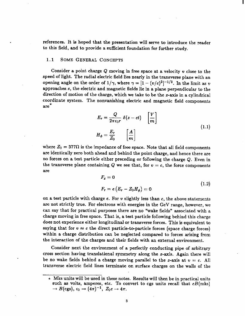
Consider a point charge Q moving in free space at a velocity u close to the speed of light. The radial electric field lies nearly in the transverse plane with an opening angle on the order of l/7, where 7 = [l - (Y/c)~]-‘/~. In the limit as 2) approaches.~, the electric and magnetic fields lie in a plane perpendicular to the direction of motion of the charge, which we take to be the z-axis in a cylindrical coordinate system.

* The nonvanishing electric and magnetic field components

are

2 - ct) [ 1 f (14 H,+=$ !! [ 1 m

where 20 = 377n is the impedance of free space. Note that all field components are identically zero both ahead and behind the point charge, and hence there are no forces on a test particle either preceding or following the charge Q. Even in the transverse plane containing Q we see that, for u = c, the force components are

F, = 0

F, = e (E, - ZoH#) = 0 (1.2)

on a test particle with charge e. For u slightly less than c, the above statements are not strictly true. For electrons with energies in the GeV range, however, we can say that for practical purposes there are no “wake fields” associated with a charge moving in free space. That is, a test particle following behind this charge does not experience either longitudinal or transverse forces. This is equivalent to saying that for u = c the direct particle-t-particle forces (space charge forces) within a charge distribution can be neglected compared to forces arising from the interaction of the charges and their fields with an external environment.

Consider next the environment of a perfectly conducting pipe of arbitrary cross section having translational symmetry along the z-axis. Again there will be no wake fields behind a charge moving parallel to the z-axis at u = c. All transverse electric field lines terminate on surface charges on the walls of the

* Mks units will be used in these notes. Results will then be in practical units such as volts, amperes, etc. To convert to cgs units recall that cB(mks) + B(cgs), Eo + (4x)-l, zoc + 47r.

3

pipe, and these charges move in synchronism with the charge or charge distri- bution on the axis. If the material in the walls of the pipe has a nonvanishing resistivity, the situation is different. The charges moving on the surface of the wall now lag slightly behind the charge on the axis. In addition, the magnetic field and the associated surface current diffuse into the interior of the metal during the passage of the bunch and decay to zero behind the bunch. Thus both longitudinal and transverse field components are now present, even behind a point charge travelling at u = c. Expressions for the wake potential for a charge moving in a cylindrical pipe with finite conductivity will be given in Section 3.2.

Consider now the more general case of a linac accelerating structure, or the discontinuities in a storage ring vacuum chamber. The individual components in the linac or vacuum chamber may have an axis of symmetry, planes of symmetry, or perhaps no symmetry at all. Suppose a unit point charge moves at the speed of light along a path, which we take to be the z-axis, through the linac or within a vacuum chamber with discontinuities. There will be no disturbance ahead of the moving charge (from causality), but behind it “wake fields” varying in a complex way in space and time will be set up by radiation from surface charges as they encounter irregularities in the wall of the structure or component. Now suppose a test charge, also moving at v = c, takes the same path through the structure or component as the unit charge, but following behind it by a fixed distance s. In general we are not interested in the details of the radiated fields due to the exciting charge, but only in their integrated effects on the test charge on passing through the component in question, or in the net effect per period in the case of a periodic structure. For a point unit charge passing through a single component we define the longitudinal delta-function wake potential W=(r) as the potential in volts per Coulomb experienced by the test particle following along the same path at time r, or at distance s = cr, behind the unit charge. For u = c, WZ(r) = 0 for r < 0 from causality. The potential at time t, in and behind an arbitrary current distribution I(t) can then be written in two alternative forms as

t 00

v(t) = J WZ(t - T) I(T) dr = J W*(T) I(t - 7) dr . (1.3) --oo 0

We see that the delta-function wake potential is a Green’s function. ‘Once. it has been computed for a given structure, the response to an arbitrary current distribution can then be readily computed. The potential V(t) within the bunch distribution is also called a wake potential. For the special case in which the total charge contained in the distribution I(t) is one Coulomb, this potential will be denoted by W (t) , with units of volts per Coulomb. The potentials V(t) and W(t) are sometimes called integrated wake potentials, since they give the integrated effect at time t of all charge elements I(t’)dt’ in the distribution which

4

have passed through the component ahead of time t. In the following sections the term “wake potential” will be used to refer to either W(t),, V(t) or W(t) whenever the context is such that there is no possibility for confusion.

The components of the wake potential may, in the general case, be both longitudinal and transverse. We may also be interested in a test particle which follows a path which is parallel to that taken by the unit charge, but displaced transversely by some specified distance. Then the components of the wake po- tential will depend on_ both the path taken by the leading charge through the cavity or structure, and also on the displaced path taken by the trailing test particle. Under some conditions (see the next section) we can also define a wake potential for particles moving at less than the speed of light. Such a wake will have a finite contribution ahead of the leading charge. But, fortunately, for high energy particles such a wake does not differ significantly from that with u = c. Since the wake potential will’ also depend on the symmetry of the structure, and on whether it is closed, open or periodic, the number of possibilities becomes quite numerous.

1.2 A NOTE ON CAUSALITY

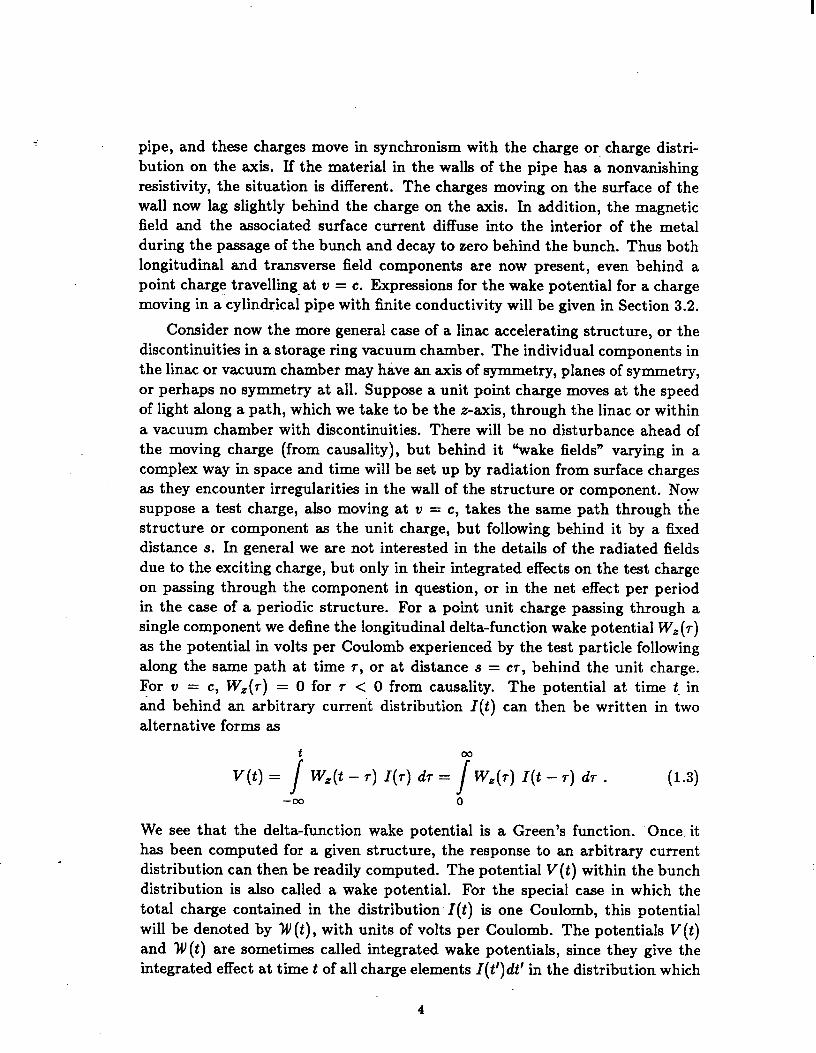
In Chapter 2 it will be shown that causality plays an important role in allowing the charge-driven wake potential to be expressed in a particularly simple way, in certain cases of special symmetry for u = c, as sums over the normal modes of the cavity or structure. For u = c the wake potential is zero for test charges moving in front of the exciting charge, from causality. But for u < c there is a finite contribution in this case. In Fig. 1 the charge Q moving along the Z- axis has passed beyond a metallic perturbing obstacle by distance ZQ. Assuming the perturbation lies close to the z-axis (b < zg), a wavefront of radiation from induced currents in the obstacle has reached a position z = ~8 + AZ, where

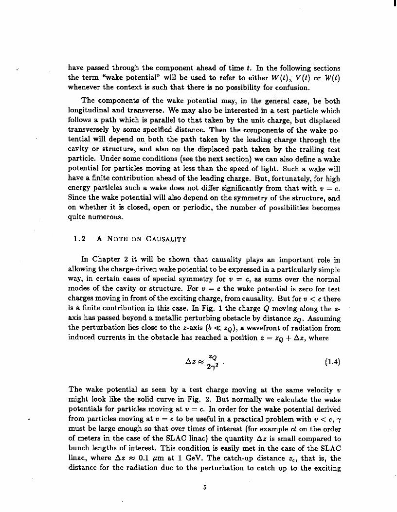
The wake potential as seen by a test charge moving at the same velocity v might look like the solid curve in Fig. 2. But normally we calculate the wake potentials for particles moving at v = c. In order for the wake potential derived from particles moving at u = c to be useful in a practical problem with u < c, 7 must be large enough so that over times of interest (for example ct on the order of meters in the case of the SLAC linac) the quantity AZ is small compared to bunch lengths of interest. This condition is easily met in the case of the SLAC linac, where AZ N 0.1 pm at 1 GeV. The catch-up distance zc, that is, the distance for the radiation due to the perturbation to catch up to the exciting

5

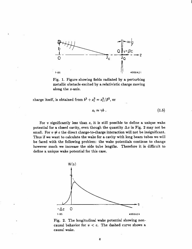
Fig. 1. Figure showing fields radiated by a perturbing metallic obstacle excited by a relativistic charge moving along the z-axis.

charge itself, is obtained from b2 + zz = z,“/p”, or

zc = 7 b. (1.5)

For u significantly less than c, it is still possible to define a unique wake potential for a closed cavity, even though the quantity AZ in Fig. 2 may not be small. For v $ c the direct charge-to-charge interaction will not be insignificant. Thus if we want to calculate the wake for a cavity with long beam tubes we will be faced with the following problem: the wake potentials continue to change however much we increase the side tube lengths. Therefore it is difficult to define a unique wake potential for this case.

W(s)

t

I -S

-AZ 0 l-85 4998A24

Fig. 2. The longitudinal wake potential showing non- causal behavior for u < c. The dashed curve shows a causal wake.

6

The effect on test particles moving behind the exciting charge gives the most important contribution to the wake potential. Let us next calculate the distance that the charge must travel before the induced radiation reaches the axis at distance s behind the charge. From the geometry of the problem we find %I = [74s2 + r2s2 + y2b2]1/2 - r2s. For s > b/y this reduces to

b2 + s2 %Q k: 2s * (l-6)

To be useful as a Green’s function, the wake potential must be accurate for values of s which are small compared to the bunch length o. For the SLAC linac, 0 kc 0.3 mm and b w 1 cm at a disk edge in the disk loaded structure. Equation (1.6) then requires that the bunch must travel 1.5 m beyond a disk before the radiation from the disk edge reaches to 0.10 behind the portion of the bunch that produced the radiation.

Recall also that if v < c the fields from a point charge have an opening angle on the order of l/7. This leads to a smearing out of the wake over a distance on the order of &b/y. At the catch-up distance z,, using Eq. (1.5), this gives a fuzziness to the wake of the order AZ = fz/y2. Note that this is of the same order as the smearing due to “causality violation” as given by Eq. (1.4).

2. NORMAL MODE EXPANSION OF THE WAKE POTENTIALS OF A CAVITY

In this chapter we show how the longitudinal and transverse wake fields can be calculated from the eigenmodes of the empty cavity. Historically a simpler, though less rigorous method employing energy conservation arguments was first used to do the same thing. Though somewhat mathematically tedious, the more direct method is employed here. It is hoped that this exercise serves to familiar- ize the reader with the old, useful though not so generally well known method for calculating the time development of fields in terms of the eigenfunctions of the empty cavity. This method is sometimes known as the Condon method.

Note that the modal method presented here is only one way of calculating the wake potential of a cavity. The other method involves direct calculation of the wake potentials by a time domain code like TBCI.“’ Normally the quickest way of getting the wake potentials of a new cavity would be to use TBCI.

7

2.1 NORMAL MODE EXPANSION OF FIELDS IN A CAVITY

The electric field E(x, t) and magnetic induction B(x,t) can be written in terms of a vector potential A(x, t) and a scalar potential Q(x, t) (in mks units) as

B =VxA

E--f+ Vi@ - at- -

In the Coulomb gauge ( V . A = 0 ) Maxwell’s equation

becomes

V=A - $s 1 i3V@ --.---Z-/&j,

c2 dt

(2-l)

(24

(2.3)

Let us restrict the domain of interest to be within a closed cavity with perfectly conducting walls. We expand the vector potential in terms of the set ax =

where

Ah, t) = c a (t)ax (4 x

(24

with V . aA = 0, and with aA x fi = 0 on the metallic surface (see for example Refs. 3 and 4). The aA are orthogonal and complete in that they can be used to compose any transverse A satisfying the metallic boundary condition at any particular instant in time. By a transverse field we mean here one with zero divergence everywhere (see Ref. 5). Similarly, we expand the scalar potential as

qx, t) = c rA(tMx(x) (2.6) x where

f-G v2+x + -@A = 0, (2.7)

with 4~ = 0 on the metallic surface. The 4~ are orthogonal and complete in that they can be used to compose any longitudinal E satisfying the metallic boundary conditions at any instant in time. By longitudinal field we mean one with zero curl everywhere. The 4~ are needed whenever source terms are present within the cavity. Note that in general WA # fI,.

8

Now substituting Eqs. (2.4) and (2.6) into Eq. (2.3) gives

C[( in + f-&&x + Wh] = p0c2j. (2.8) x

Dotting Eq. (2.8) with aAl and integrating over the cavity volume U gives

(tAt + wt,qxl) J ax1 . axdV + +A# J ax) - V4xdV = poc2 J j - wdv- (2.9) v _ V V

The second integral of Eq. (2.9) can be written as

J aAt - V+xdV = J V - (&ap)dU - J &(V. axl)dV. (2.10) V V V

The first integral on the right of the above equation vanishes since 4~ = 0 on the boundary (by the divergence theorem); the second term vanishes since the Coulomb gauge is used. Thus if we normalize the aA as

CO

z J ap - axdV = U~S~p, (2.11) V

where 6xx, is the Kronecker delta, Eq. (2.9) becomes simply

1 ix +w;qx = -

2ux J j -axdV. V

(2.12)

Note that whenever there is no current in the cavity the qx vary sinusoidally at frequencies WA (if they are not identically zero). In this case A can be written as

A(x, t) = c Cxax cos(qt + 0,) (2.13) x

where the CA and 6~ are constants depending on how the modes were generated. Therefore we see that the aA are the eigenmodes of the empty cavity and the corresponding WA are the resonant frequencies.

Similarly, beginning with

V.&f CO

we get 1

rA = 2TA -J/cwv . V

(2.14)

(2.15)

9

if the 4~ are normalized by

CO

-ii J V& 9 V4AdV = TxSxAt. (2.16) v

Whenever there are no charges in the cavity, all the r~ (and thus also a) are zero.

Thus, given the homogeneous solutions ax, q5~ and the sources j, p, we can solve for the qA,rA from Eqs. (2.12) and (2.15). These in turn allow us to solve for E and B by way of Eqs. (2.1), (2.4) and (2.6). The electric field is given by

E = - x(im + rxbh) x

(2.17)

and the magnetic induction is

B=&Vxax. x

The stored energy is given by

& = ; J (coE2 + B2/po)dV V

= C( &JA + w$$T~ + #A). x

(2.18)

(2.19)

In deriving Eq. (2.19) we have used the fact that

J (V xap)-(Vxax)dV = J V-(ax,x(Vxax))dV+ J ap.(VxVxax)dV (2.20) V V V

where the first integral on the right vanishes since ax) x d = 0 on the boundary.

2.2 THE LONGITUDINAL WAKE POTENTIAL

.

Consider any closed, empty (vacuum, no sources) cavity with perfectly con- ducting walls. An exciting particle with charge Q traverses the cavity at velocity u = c. We arrange our axes such that this charge enters the cavity at z = 0 at time t = 0 and follows along the z-axis. It leaves at z = L. The longitudinal

10

wake potential W, (more precisely, the delta-function longitudinal wake poten- tial) is defined as the total voltage lost by a test charge following at a distance s on the same path and also at v = c, divided by Q. Thus

We(s) = -$ f dz E&, (% + 4/c) 0

(2.21)

where E,(z, t) is the z component of E on the z-axis due to the exciting charge. Note that since a signal cannot travel faster than the speed of light W, = 0 for s < 0.

As mentioned in the Introduction, the usefulness of this definition is that W, can be used as a Green’s function for computing the voltage loss within an ultra- relativistic bunch of arbitrary shape. W,, the voltage loss per unit total charge, is also called the wake potential, or sometimes the bunch wake to differentiate it from W,. The two wakes are connected by

W,(s) = 7 ds’ I’(s - s’) W&‘), 0

(2.22)

where I’(s) is the charge distribution of the bunch. Note that cl’(s) simply equals the current distribution I(s/c) used in the Introduction. Approximating the bunch as rigid is normally valid since a high energy beam does not change its shape much over the distance of a cavity. Approximating the speed as u = c is valid since the wake fields of a cavity turn out to be independent of the energy of the bunch at high energies. This approach differs greatly from the more difficult method (which still needs to be done for low energy beams) of self consistently solving for the fields in the cavity and the beam motion.

To calculate W, we need first to find the fields in the cavity due to the exciting charge. The source terms due to the exciting charge are

p-(x, t) = Q+)~(Y)+ - ct) (2.23)

j(x, t) = iicp(x,t).

Eq. (2.12) becomes

0 t<o Qc qx + +A = z adW, 4 0 < t < L/c

0 . t > L/c,

(2.24)

where axz(z, y, z) is the z-component of ax. Using initial conditions q(0) = i(O) = 0 ( no e fi Id s in the cavity before the charge enters) and by variation of

11

parameters, we get

9AP) = &

Similarly substituting (2.23) into (2.15) we get

min(t,l/c)

J dt’sin wx(t 0

t’) aA,(O, 0, ct’).

Q rx(t) = 2~ i

f$x(O,O,ct) 0 < t < L/c x

0 t > L/c

(2.25)

(2.26)

where the three arguments of 4~ represent respectively its x, y and z dependence. With the above two equations and Eqs. (2.17)-(2.19) we can construct the fields and stored energy due to the exciting charge for all time solely in terms of the empty cavity solutions aA, 4~) WA.

From Eqs. (2.19) and (2.25) we see that the energy left in the cavity after the exciting charge has left (t > L/c) is

& = c (a! + &I:) VA x

=Q2F&

where L

VA = J dz exp(iwxz/c) axz(O, 0, z). 0

Defining the loss factor kx as

kA = A2 ‘,“u’ x

(2.27)

(2.28)

(2.29)

the stored energy becomes simply

& = Q2xkx. x

(2.30)

Thus kx gives the amount of energy deposited in mode A by the exciting charge, hence the name loss factor.

12

The variables on the right side of Eq. (2.29) defining kx can be given the following physical interpretation: Suppose mode X of the empty cavity has been excited by any method whatever. From the definition of VA (see Eq. (2.11)) we see that it can represent the energy stored in this mode, up to a multiplicative constant. If now a test charge traverses the cavity at u = c along the z-axis, then lV’12 can be thought of as the square of the maximum voltage it can gain (with respect to time of entry) from this mode, up to the same multiplicative constant. Thus, just like the eigenfrequency WA, kx is a property of the empty cavity depending on its shape. Unlike WA it depends also on the integration path used for calculating VA.

Now we continue our calculation of the wake potential in terms of the normal mode solutions of the cavity. The calculation becomes somewhat tedious, but the results turn out to be of a rather simple form. Combining Eqs. (2.17) and (2.21) yields

W=(s) = $x jdr [dA (1:_b) qJO,o,z) +rx (F) $(o,o,z)]. x 0

(2.31) (Henceforth we shall use the shorthand aAz (z) to represent aAz (0, 0, z) and sim- ilarly for 4x.) Substituting for qx, rA from Eqs. (2.25) and (2.26) gives us our final results. The problem is naturally solved in three pieces:

a) s > L: The test charge enters after the exciting charge has already left the cavity. We get

W=(s) = F g s > L,

with L L

h(s) = J J d% dy 4%) ax,(y) 0 0

= Re {ViVx exp(iwxs/c)} .

Eq. (2.32) can be rewritten as

W=(s) = c 2kx CQS f$f x

(2.32)

cosy%+s-y) (2.33)

s > L. (2.34)

b) 0 < s < L: The test charge enters while the exciting charge is still in the

13

cavity. Here

w&) = c ( 2uA h(s) - Izx(s) + k(s)

x 27” ) o<scL’

where

-L-s L

Izx(s) = dz J J dy a&) ax,(y) ~0s y(% + s -.Y) 0 Z‘+B

and

L-s

h(s) = J dz z(z) +A(% + s). 0

(2.35)

(2.36)

(2.37)

We have used the relation

[r”% py.1 d,),,] f(w) = [ydlydv- ~%~dv] f(w)

(2.38) in Eq. (2.35).

From causality we know that the wake potential is zero for s < 0. In particular, in the range -L < s < 0 we get the relation

13x(s) K2x(s) W=(s) =x(x+ 2Tx ) =o -L--CO, (2.39) x

where

L Z+8

133x(s) = dz J J dy 4%) aAz (y) co2(%+s-y) -8 0 L+s L

J J dz dy a&) alz (y) (2.40) = COSfy%-s-y)

0 Z-8 .

= 12x(-s)

14

and L

Kzx(s) = J dz “’ -&4 4x(% + s) -8

L

=- J dz g(%+S) h(%> -8 (2.41)

L+s =- J dz z(z) 4&z - s)

0

= - &x(-s).

We have integrated by parts to go from the first to the second expression for Kzx, using the fact that 4~ = 0 on the boundary. Thus relation (2.39) can be rewritten as

12x(4 K2xb) m- 2TA = >

o O<s<L.

Therefore Eq. (2.35) becomes simply

W=(s) = F g O<s<L.

= c 2kx cos f!? n

(2.42)

(2.43)

c) s < 0: The test charge enters before the exciting charge. From causality

W=(s) = 0 9s < 0. (2.44)

What about the point s = O? W=(O) can be interpreted as the voltage the exciting charge itself loses to the cavity, divided by its charge Q. From Eq. (2.30) we see that its voltage loss to mode X is just k,Q. These results can be summarized as

W=(s) = xkAcosy 1 s = o x 2 s>o.

(2.45)

Note that due to the symmetry introduced by taking the velocities to be c, W, does not depend on the scalar potential solutions C$X, even if the test charge enters while the exciting charge is still in the cavity (0 < s < L). For v $ c

15

however, the scalar potential solutions can become important. W, then becomes very complicated, and the general usefulness of the wake potential concept is lost. Note also that, since W, is expressable as a sum of cosines, its maximum value is at s = O+.

2.3 THE TRANSVERSE WAKE POTENTIAL

Consider again the exciting charge Q traversing the closed, empty, perfectly conducting.cavity at v = c. Again it enters at z = 0, follows along the z-axis, and leaves at z = L. The transverse wake potential WI is defined as the transverse momentum kick experienced by a test charge following at a distance s on the same path and also at u = c, divided by Q. (Note that WI is a vector with both x and y components.) Thus

L

w,(s) = $ J d% [El + (v x %1t=(z+,)/c 0

L

= ; J dz [h(v . A) - (; + v . V)h - vlqt+++ 0

L L,t=(L+s)/c

= $ d% [cvdz - V.P%=(z+s)/c - $&lo t=s,c J . ,

0

(2.46)

In Eq. (2.46) all x and y arguments are set to zero. For cavities with walls perpendicular to the z-axis at z = 0 and z = L the boundary terms in Eq. (2.46) vanish. We will drop these in the following. (They can always be added at the end.) Thus (2.46) becomes

L 1

Wh) = ij J d% [cVIA, - Vd]t++s)/c . (2.47) 0

Analogously to the longitudinal case, WI can be used as a Green’s function for transverse momentum kick per total charge within an ultra-relativistic bunch of arbitrary shape, which we denote by $L. $L is given by

Ii&(s) = /m ds’ l’(s - s’) Wl(S’), 0

(2.48)

where I’(s) is the charge distribution of the bunch.

16

Substituting Eqs. (2.4) and (2.6) into Eq. (2.47) we get

W,(s) = $gdl [.,A (F) VlUA&) -f-A (f$) VLh(Z)] *

(2.49) Then substituting for qA,rA from Eqs. (2.25) and (2.26) gives us the transverse wake purely in terms of the aA and 4~. Again solving the problem in three pieces gives:

a) s > L: The test charge enters after the exciting charge has already left the cavity. We get

W,(s) = F f-$g s > L, (2.50)

with

L L

k(s) = / /

dz dy (VLU&>) Q(Y) sin y(z + s - Y) 0 0 (2.51)

= Sm {Vx*VlVx exp(iwxs/c)} .

b) 0 < s < L: The test charge enters while the exciting charge is still in the cavity. Here

W(s) = c (c I:,(s) - %(s) _ K:,(s) 2wQ 2% > O<s<L, (2.52)

x

where

L-s L

dy (Vm&)) U(Y) sin y(z + s - Y) (2.53)

0 Z+S

and L-8

G(S) = I

dz (hh(4) h(z + 4. (2.54)

0

From causality we know that the wake potential is zero for s < 0. In

17

particular, in the range -L < s < 0 we get the relation

W,(s) = c (c!i& - K;g’) = 0 - L < s < 0, x

(2.55)

where L e+.¶

Iix(s) = dz / /

dy (&me(z)) Q(Y) sin y(z + s - y) -8 0

&+8 L (2.56)

=- / /

dz 4/ ax&) VPA,(Y) sin y(z - s - Y) 0 Z-8

and L

K12Xb) = / dz m4x(4) 4A(Z + s) -8 L+s

(2.57)

= / dz (Vdx(z - 4) +A(+ 0

Unlike the longitudinal case, Eq. (2.52) cannot in general be simplified. We will see below that in certain special cases Eq. (2.55) along with Eqs. (2.56) and (2.57) can be used to simplify the form of WI for 0 < s < L.

c) s < 0: The test charge enters before the exciting charge. From causality

Wl(S) = 0 s < 0. (2.58)

Observing Eqs. (2.53), (2.54), (2.56), and (2.57) we see that there is a certain similarity between Iix and IL,, and between Ki, and KLx. For the special case of a right cylinder with arbitrary cross-section whose axis is aligned with the z-axis ax= can be written as

%(G Y> 4 = fx(T Yh(Z) (2.59)

and similarly for 4~. In this case

&x(s) = -&J-s) O<s<L,

Km = w-4 (2-W)

and relation (2.55) becomes

o O<s<L. (2.61)

Combining Eq. (2.61) with Eq. (2.52) we see that WI for 0 < s < L has the

18

identical form as over the range s > L. Therefore we get

W,(s) = ~cv~~~~ sin? s>o x

(2.62)

for cavities with translational symmetry along the z-axis. We see that the ex- citing charge itself feels no wake field. Since the transverse wake is a sum of sine terms it rises to a maximum value somewhere behind the exciting charge.

2.4 FURTHER GENERALIZATIONS

The wake field definitions given in Sections 2.2 and 2.3, valid for u = c, can be extended somewhat. For high energy particles (u M c) the wake field concept is still useful. The exercise of the previous two sections can be repeated for such a case, yielding somewhat more complicated results. Generally the correction terms to the wake fields are proportional to rv2, where 7 is the particle energy (see Ref. 6). But as pointed out previously, for low energy particles the wake field concept loses its usefulness. In this regime one needs to solve the complete self- consistent problem where the fields created by the particles change the particles’ motion which again changes the fields.

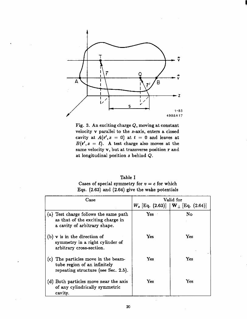
Another generalization already mentioned in the Introduction is to define the wake fields in terms of an exciting charge and a test charge that move on parallel paths, not merely on the identical path. Let us take those paths to be parallel to the z-axis. Then the wake fields are functions of r’ and r where these are the transverse coordinates, respectively, of the exciting charge and the test charge, as well as of their longitudinal separation s as shown in Fig. 3. For many practical problems the r’,r dependences of the wake fields are of a simple form and can be solved independently of the s dependence.

For the special case of cavities with translational symmetry, that is, those for which a~, can be written as in Eq. (2.59), the methods used in Sections 2.2 and 2.3 yield

WAS W,(r’, r, s) = C vT(ic(r) ~0s c s>o x

(2.63)

and

Wl(r’,r,s) = Cc Vx*(r’PLT’x(r) WAS 2G4Jx

sin - s > 0. (2.64) x C

Table I gives a summary of some cases of special symmetry where the longitu- dinal and transverse wakes are given by the above equations.

19

A\ 4

\ I ’

I \

II’ ’ / -2 I /

lr s VW l-85

J 4990Al7

Fig. 3. An exciting charge Q, moving at constant velocity v parallel to the z-axis, enters a closed cavity at A(r’,z = 0) at t = 0 and leaves at B(r’,z = e). A test charge also moves at the same velocity v, but at transverse position r and at longitudinal position s behind Q.

Table I Cases of special symmetry for u = c for which

Eqs. (2.63) and (2.64) give the wake potentials

Case Valid for W, [Eq. (2.63)] WI [Eq. (2.64)]

(a) Test charge follows the same path Yes No as that of the exciting charge in a cavity of arbitrary shape.

(b) v is in the direction of symmetry in a right cylinder of arbitrary cross-section.

Yes Yes

(c) The particles move in the beam- tube region of an infinitely repeating structure (see Sec. 2.5).

Yes Yes

(d) Both particles move near the axis of any cylindrically symmetric cavity.

Yes Yes

20

Equations (2.63) and (2.64) are related by the expression

awL -= CYS

v w I z * (2.65)

The above expression is sometimes termed the Panofsky-Wenzel theorem.“’ The theorem follows directly from Eq. (2.47) if the scalar potential term is set to zero. It was originally derived to calculate the transverse momentum kick received by a nonperturbing charge traversing a cavity excited in a single rf mode. In that case the field and wake potentials are derived from the vector potential alone.

2.5 INFINITELY REPEATING STRUCTURES

Real linear accelerator structures are finite, but infinitely repeating struc- tures are often easier to solve than finitely repeating ones. With many cavities the effects of end plates on the wake potential per cell become negligible (for - - s # 0), and the infinite solution closely approximates the finite case.

Consider an infinitely repeating structure with period p that repeats in z direction. From the Floquet condition we know that in such a structure must satisfy the condition

a&, z + p) = eiplpuxZ(r, z),

the ah

where r = x% + & and /?xp is an arbitrary phase advance per cell. We can therefore expand a~= in a Fourier series as

ax=(r,z) = eiPxz C fXn(r)etninzlp. n=--OO

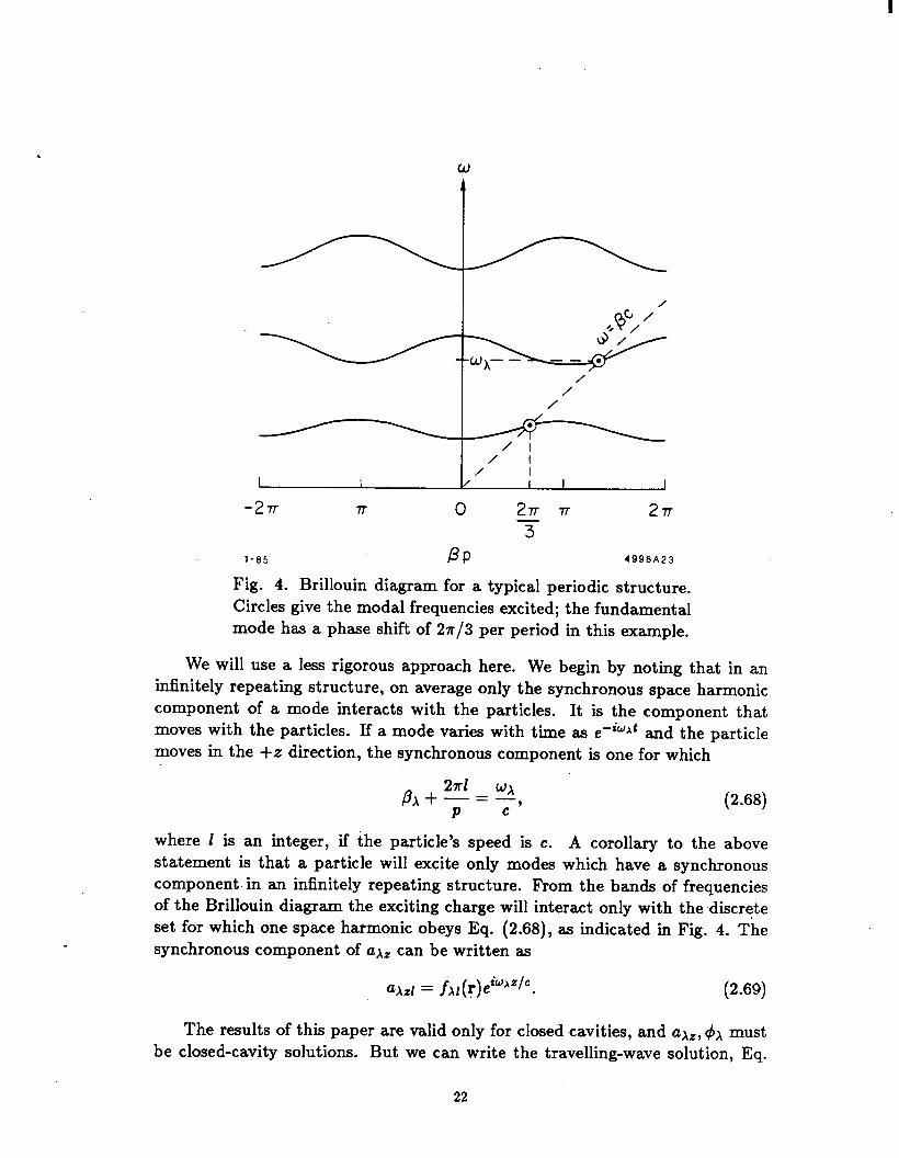
The terms in the sum are sometimes called the space harmonics. Rather than the discrete resonant frequencies WA of a closed cavity, in an infinitely repeating structure the eigenfrequencies come in bands depending on the phase advance per cell ,Oxp (see for example Ref. 8). An example of an WA vs pip plot -for such a structure, also called a Brillouin diagram, is given in Fig. 4.

The wake potentials for an infinitely repeating structure can be obtained by the methods of Sections 2.1, 2.2, and 2.3. We first need to modify the method of expanding the electric and magnetic fields in terms of the eigenmodes to include vector and scalar potentials in complex form. The wake fields can then be obtained by the methods of Sections 2.2 and 2.3,‘although the solution is quite tedious (see for example Ref. 9).

21

-27T 77 0 27T 7T 277 3

l-85 PP 4998A23

Fig. 4. Brillouin diagram for a typical periodic structure. Circles give the modal frequencies excited; the fundamental mode has a phase shift of 2x/3 per period in this example.

We will use a less rigorous approach here. We begin by noting that in an infinitely repeating structure, on average only the synchronous space harmonic component of a mode interacts with the particles. It is the component that moves with the particles. If a mode varies with time as eBiwxt and the particle moves in the +z direction, the synchronous component is one for which

where I is an integer, if the particle’s speed is c. A corollary to the above statement is that a particle will excite only modes which have a synchronous component. in an infinitely repeating structure. From the bands of frequencies of the Brillouin diagram the exciting charge will interact only with the ,discrete set for which one space harmonic obeys Eq. (2.68), as indicated in Fig. 4. The synchronous component of a~= can be written as

a~,! = fAl(y)eiwAalc. (2.69)

The results of this paper are valid only for closed cavities, and ax=, 4~ must be closed-cavity solutions. But we can write the travelling-wave solution, Eq.

22

(2.69), as the sum of two out-of-phase standing wave solutions,

w = h(r) ( cos wxz/c + i sin w~z/c) . (2.70)

Since L = 00 in an infinitely repeating structure, we are always in the region 0 < s < L when the exciting charge is in front of the test charge. Since Ural, 4x1 are of the form of Eq. (2.59), we can use Eq. (2.63) giving

W,(r’, r, s) = C p2 fA’(:gA’(rJ cos y s>o x x

per period p, since

NP/~

Jim, f + / dz cosw~z/c eiwAZ/’ = p/2

-NP/~

(2.71)

(2.72)

and half the energy is stored in each standing wave. In Eq. (2.71) the sum is restricted to those modes that have a synchronous space harmonic. As in the previous section r’ and r represent respectively the transverse position of the exciting charge and the test charge. Similarly, for the transverse wake field we get

W&‘,r,s) = CCP 2 fdr’)hh(r) sin WAS s>o (2.73)

x 2m4 C

per period.

Let us now restrict our interest to cylindrically symmetric structures. We will now use polar coordinates (r,t9) to denote transverse position. The exciting charge traverses at r = r’, 6 = 0 (on the z-axis). Let the tube radius of the structure be denoted by a (see Fig. 5a). In such a structure all the modes depend on 8 as eim8, where m is an integer. The m = 0, 1,2 modes are called respectively the longitudinal, dipole, quadrupole modes. Further it can be shown that for a particle moving at u = simply P. ‘1o1

c the t dependence of the function fxl(r) is Therefore the m-pole component of the wakes can be written as

a sum over all the m-pole modes as

(2.74)

while for m # 0

W # m r m-l

Im=m ; a 0 (1

(P cos m6-8 sin me) C ~~nf~~) n (

sin ff!?ff s > 0.

(2.75) For m = 0, WI, = 0. In the above equations lcmn(o) is the loss factor calculated

23

at r = a. We can summarize the relationship between the components as

Lw*m = v,w,, . (2.76)

Note that this is identical in form to Eq. (2.65)

(a)

(b) t-p-l t-1

(cl t-1 --- -

I -- -r

I- lAa p

I I I I :4QQW3 l-05

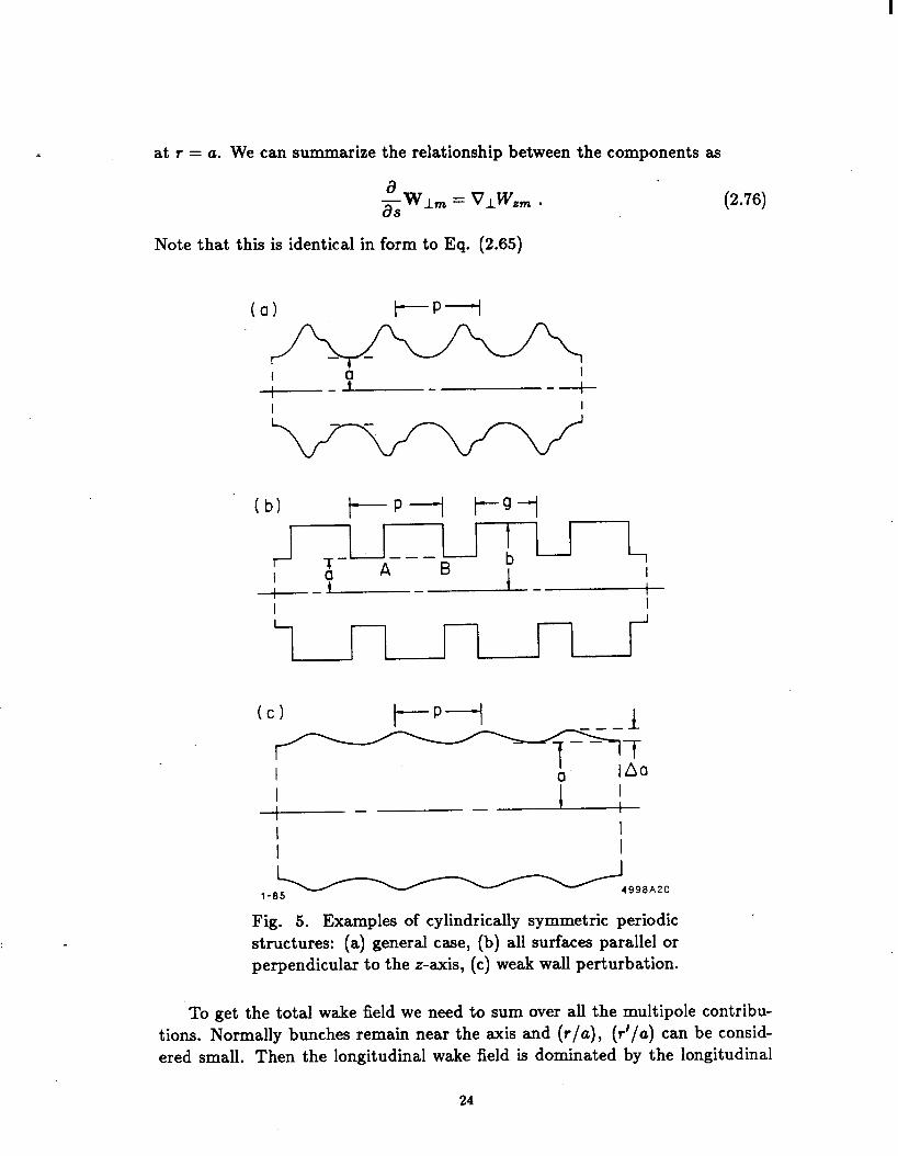
Fig. 5. Examples of cylindrically symmetric periodic structures: (a) general case, (b) all surfaces parallel or perpendicular to the z-axis, (c) weak wall perturbation.

.

To get the total wake field we need to sum over all the multipole contribu- tions. Normally bunches remain near the axis and (r/u), (r’/u) can be consid- ered small. Then the longitudinal wake field is dominated by the longitudinal

24

modes (m = 0) whereas the transverse wake field is dominated by the dipole modes (m = 1). Thus normally we can approximate the wakes as

Wz N ELkon COS y S > 0 n

WI= r ’ -( ) ; 2 c

2hn(a) . WlnS

n (Wna/c) “Il C s > 0.

(2.77)

(2.78)

Note that the longitudinal wake is approximately independent of the transverse position of both the exciting charge and the test charge. The transverse wake depends on the exciting charge as the first power of its offset. The transverse wake is in the z-direction and is independent of the test charge’s transverse position.

Sometimes one is interested in the wake potential of a single cavity with beam tubes. If we take an infinitely repeating structure, increasing the tube length between the cells, we can imagine that the wake potential per cell of the repeating structure will approach the total wake potential for a single cavity with long beam tubes. For proof that Eq. (2.76) as well as the r, 8 dependencies of Eqs. (2.74) and (2.75) hold for a single cylindrically symmetric cavity see Ref. 11.

2.6 THE WAKE FIELDS FOR THE SLAC STRUCTURE

The longitudinal and transverse wake potentials per cell have been computed”” for the SLAC disk-loaded accelerating structure using a summation over nor- mal modes according to Eqs. (2.77) and and (2.78). This computation offers a practical example of the usefulness of the modal development of the preceding sections.

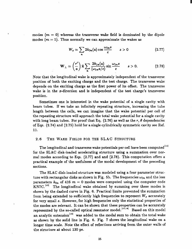
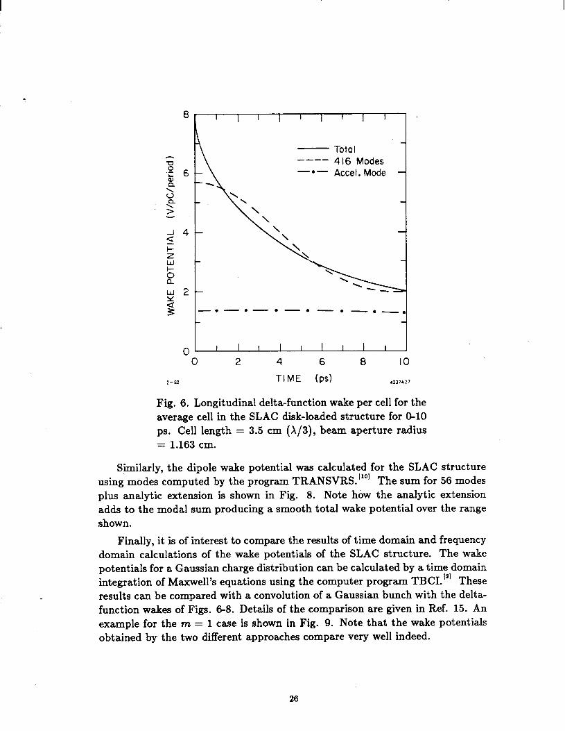
The SLAC disk-loaded structure was modeled using a four parameter struc- ture with rectangular disks as shown in Fig. 5b. The frequencies won and the loss parameters ken of 416 m = 0 modes were computed using the computer code KN7C.“” The longitudinal wake obtained by summing over these modes is shown by the dashed curve in Fig. 6. Practical limits prevented the summation from being extended to sufficiently high frequencies to represent W, accurately for very small s. However, for high frequencies only the statistical properties of the modes are relevant. It can be shown that these properties can be accurately represented by the so-called optical resonator model.“s’*4’ Based on this model an analytic extension ‘12’ was added to the modal sum to obtain the total wake as shown by the solid line in Fig. 6. Fig. 7 shows the longitudinal wake on a longer time scale. Note the effect of reflections arriving from the outer walls of the structure at about 130 ps.

25

u .- ; 6 a 3 n >

I I I I 1 I I I I

- Total ---- 416 Modes -*-- Accel. Mode

l-81 TIME (PSI 4137*17

Fig. 6. Longitudinal delta-function wake per cell for the average cell in the SLAC disk-loaded structure for O-10 ps. Cell length = 3.5 cm (X/3), beam aperture radius = 1.163 cm.

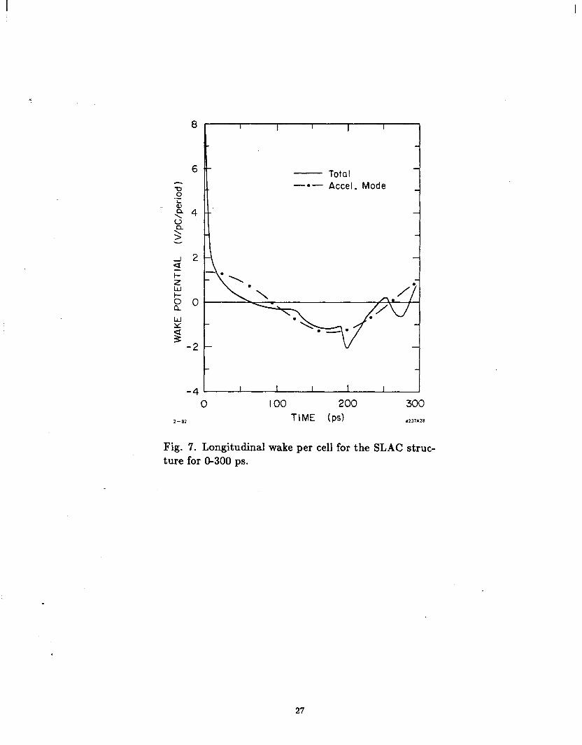
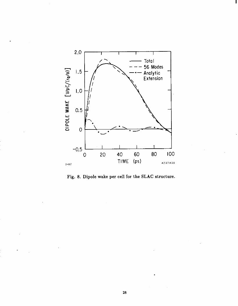
Similarly, the dipole wake potential was calculated for the SLAC structure using modes computed by the program TRANSVRS.“” The sum for 56 modes plus analytic extension is shown in Fig. 8. Note how the analytic extension adds to the modal sum producing a smooth total wake potential over the range shown.

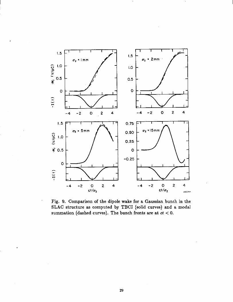
Finally, it is of interest to compare the results of time domain and frequency domain calculations of the wake potentials of the SLAC structure. The wake potentials for a Gaussian charge distribution can be calculated by a time domain integration of Maxwell’s equations using the computer program TBCI.‘“’ These results can be compared with a convolution of a Gaussian bunch with the delta- function wakes of Figs. 68. Details of the comparison are given in Ref. 15. An example for the m = 1 case is shown in Fig. 9. Note that the wake potentials obtained by the two different approaches compare very well indeed.

26

- Total --a- Accel. Mode

-4 0 100 200 300

2-81 TIME (ps) 4237A18

Fig. 7. Longitudinal wake per cell for the SLAC struc- ture for O-300 ps.

27

F 1.5

w z 3 0.5

- Total - - - 56 Modes

3-82 TIME (ps) 4237A30

Fig. 8. Dipole wake per cell for the SLAC structure.

.

28

1.5

z 1.0 Q 5 yL 0.5 &

0

w I

1.5

G e 1.0 >

g- 0.5

0

l-4 I

I I I I I

I I I I I 1

I 1-r

-4 -2 0 2 4

-4 -2 0 2 4 cth7~

1.5

1.0

0.5

0

-4 -2 0 2 4

0.75

0.50

0.25

0

-0.25

-4 -2 0 2 4 ct/cT, rr53*r

Fig. 9. Comparison of the dipole wake for a Gaussian bunch in the SLAC structure as computed by TBCI (solid curves) and a modal summation (dashed curves). The bunch fronts are at ct < 0.

29

3. ANALYTIC CALCULATIONS OF WAKE POTENTIALS

3.1 SEMI-INFINITE RESISTIVE SLAB

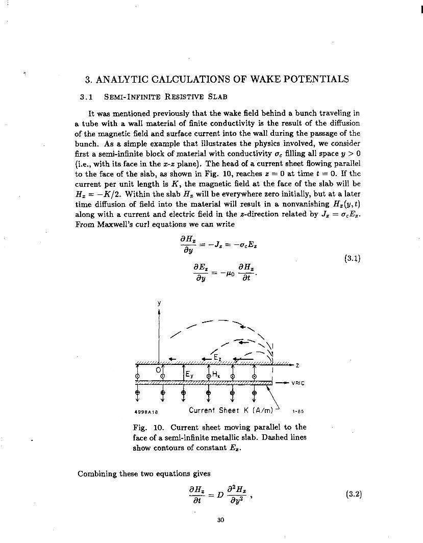
It was mentioned previously that the wake field behind a bunch traveling in a tube with a wall material of finite conductivity is the result of the diffusion of the magnetic field and surface current into the wall during the passage of the bunch. As a simple example that illustrates the physics involved, we consider first a semi-infinite block of material with conductivity cre filling all space y > 0 (i.e., with its face in the x-z plane). The head of a-current sheet flowing parallel to the face of the slab, as shown in Fig. 10, reaches z = 0 at time t = 0. If the current per unit length is K, the magnetic field at the face of the slab will be Hz = -K/2. Within the slab H, will be everywhere zero initially, but at a later time diffusion of field into the material will result in a nonvanishing H,(y,t) along with a current and electric field in the z-direction related by Jz = a,E,. From Maxwell’s curl equations we can write

aHz -J -= aY

- -a,E, Z-

aEz a&

- = -IJo at’ aY

(3.1)

4990A10 Current Sheet K (A/m) ’ l-85

Fig. 10. Current sheet moving parallel to the face of a semi-infinite metallic slab. Dashed lines show contours of constant Ez.

Combining these two equations gives

a& D a2Hz -= P at ay2 ’ (34

30

where D is the diffusivity D = l/pea, in m2/sec. The solution satisfying H,(O, t) = -K/2 is”‘]

H,(y,t) = -; 1 { -erf [(4Di)‘ialJ *

The longitudinal electric field is now obtained as

E,(y,t) =--; f.$ = - K

2c7,(7rDt)l/2 exp Y2 [ 1 --

4Dt ’

(3.3)

(3.4

Setting y = 0 gives Ez at the surface and, by continuity, outside the slab. Equation (3.4) is the solution for Ez due to a current step applied at t = 0.

The solution for a rectangular pulse of current can be obtained by adding to Eq. (3.4) the solution for a current step of equal magnitude but opposite sign which is delayed by time At. Carrying out this operation for y = 0 results in

E,(O,t) za F l/2

t-3/2 , (3.5) where Ql = KAt is the charge per meter in the pulse.

Note that the wake in Eq. (3.5) is accelerating and therefore cannot be valid for t --+ 0. In any case, the displacement current has been ignored in Eq. (3.1). Th e is d pl acement current and conduction current within the slab become comparable at times on the order of t - ce/~~. For times which are short compared to this, the diffusion equation, Eq. (3.2), must be replaced by the wave equation. The solution to the boundary value problem then leads to a retarding field at the position of the charge.

-3.2 CYLINDRICAL PIPE WITH RESISTIVE WALLS

The delta-function wake potential for a point charge moving in a cylindrical pipe with a resistive wall is calculated in Refs. 17 and 18. The mathematics is relatively complex and will not be repeated here. The basic physical principle of diffusion of fields into the material, which then decay to zero behind the bunch, still applies however. In this section we take the results of Ref. 18, which are in Gaussian units, and rewrite them in practical units.

The longitudinal electric field at distance s behind a point bunch of charge Q moving on the axis of a cylindrical pipe with radius b and conductivity oc is

l/2 s-312 . P-6)

Note that Ez is uniform throughout the pipe; that is, it does not depend on radial position behind the bunch. This expression is, however, valid only for

31

distances s which are large compared to a critical distance SO given by

P-7)

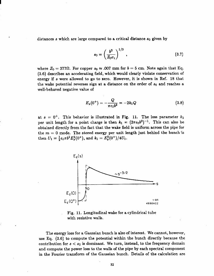
where 20 = 377$-I. For copper SO w .007 mm for b = 5 cm. Note again that Eq. (3.6) describes an accelerating field, which would clearly violate conservation of energy if s were allowed to go to zero. However, it is shown in Ref. 18 that the wake potential reverses sign at a distance on the order of SO and reaches a well-behaved negative value of

Jqo+) = --J&$ = -2klQ

at s = O+. This behavior is illustrated in Fig. 11. The loss parameter kl per unit length for a point charge is then kl = (2?rcob2)-‘. This can also be obtained directly from the fact that the wake field is uniform across the pipe for the m = 0 mode. The stored energy per unit length just behind the bunch ‘is then Ur = ~corb2E~(O+), and kl = E~(O+)/4U1.

E,(s)

l-95 4999A22

Fig. 11. Longitudinal wake for a cylindrical tube with resistive walls.

The energy loss for a Gaussian bunch is also of interest. We cannot, however, use Eq. (3.6) to compute the potential within the bunch directly because the contribution for s < so is dominant. We turn, instead, to the frequency domain and compute the power loss to the walls of the pipe by each spectral component in the Fourier transform of the Gaussian bunch. Details of the calculation are

32

given in Ref. 19. The result is

(3.9)

where ICI is in volts per Coulomb per meter. Putting in constants, this becomes

k&J = 1.28 x lo8 ' -m 1 1 c - fpl2 b3/20v * z C

(3.10)

Applying this expression to compute the loss by a bunch of 10" electrons trav- eling the length of the SLAC linac (3 km) in aluminum pipe 5 cm in radius, we find an energy loss eklQL = 0.6 MeV for a, = 1 mm.

The dipole resistive wall wake in a cylindrical pipe is also obtained from Ref. 18 as

El(S) = g (g) 112

d2 . c

(3.11)

The dipole wake potential is then W_L(S) = El(s)/Q. Using this wake to com- pute the deflecting field in a Gaussian bunch centered at s = 0 we obtain

El(S) =

where F is a universal function of s/a, given by

F (;) = &==Jex$---~;~) ds’ .

(3.12)

(3.13)

In computing the wake potential per unit length given by Eq. (3.12), we do not need to take into account. the fact that Eq. (3.11) is not valid for s < se, as long as oZ >> se. This so because the transverse wake does not change sign at SBYsg( it a s fll t o zero for s < SO), and because it decreases more slowly at long distances compared to the longitudinal wake (~~~1~ vs sS3i2).

33

3.3 PILLBOX CAVITY

The longitudinal and transverse wake potentials produced by a charge pass- ing on the axis of a cylindrically symmetric pillbox cavity can be computed in terms of the mode frequencies WA and loss parameter values kx, using the formalism developed in Chapter 2. For longitudinal modes the frequencies are obtained from

WjP - (g2+ (7)’ . (3.14)

Here R is the cavity radius, g is the cavity length, j,, is the nth zero of JO(Z) and the index p gives the longitudinal variation of the axial electric field,

(Ez)np - J0 (jn k) cos (7) exp(hpt) . (3.15)

The delta-function wake potential is calculated (see for example Ref. 20) as .

K(s) = (3.16)

where cp = l/2 for p = 0, cp = 1 for p # 0. If s is set to zero in the preceding relation, the sum diverges with increasing mode number, although only logarith- mically. Thus a point charge passing through a completely closed pillbox suffers an infinite energy loss. For a Gaussian charge distribution this is no longer the case. The potential at position z for a bunch centered at z = 0 is given by’2!

(3.17) where w(z) is the complex error function and Be stands for the real part. No closed expression is known for this sum, but it has been evaluated numerically for sample cases and is found to agree well with results calculated by the time domain program TBCI.

For s < (4R2 + g 2 ‘i2 - g the sum in Eq. (3.16) for the delta-function wake ) can be evaluated analytically. For the above range of s no wave created by the leading charge can reach the outer cylindrical wall of the cavity, be reflected and arrive back at the test charge before it has left the cavity. The pillbox cavity wake therefore looks identical to the wake for two infinite parallel plates over

34

this range of s. Over this range of s it can be shown that ‘20-221

27rroK(s) = 26(s) ln (i) - 2 e J&w - s) In [(s + ,P;, _ g,] n=l

(3.18) 1 -- 9

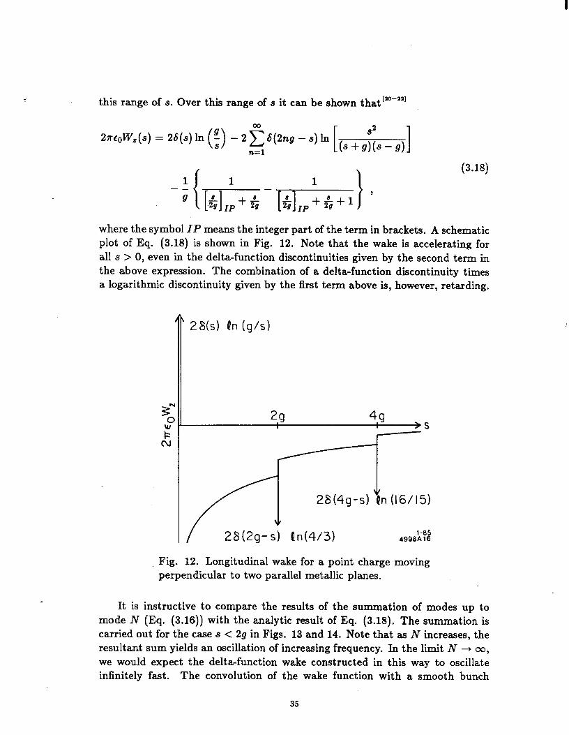
where the symbol IP means the integer part of the term in brackets. A schematic plot of Eq. (3.18) is shown in Fig. 12. Note that the wake is accelerating for all s > 0, even in the delta-function discontinuities given by the second term in the above expression. The combination of a delta-function discontinuity times a logarithmic discontinuity given by the first term above is, however, retarding.

26(s) Qn (g/s)

/ 28(2g-s) th(4/3) l-85 4996A16

Fig. 12. Longitudinal wake for a point charge moving perpendicular to two parallel metallic planes.

It is instructive to compare the results of the summation of modes up to mode N (Eq. (3.16)) with the analytic result of Eq. (3.18). The summation is carried out for the case s < 2g in Figs. 13 and 14. Note that as N increases, the resultant sum yields an oscillation of increasing frequency. In the limit N + 00, we would expect the delta-function wake constructed in this way to oscillate infinitely fast. The convolution of the wake function with a smooth bunch

35

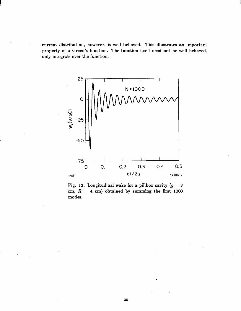
current distribution, however, is well behaved. This illustrates an important property of a Green’s function. The function itself need not be well behaved, only integrals over the function.

25

0

-50

-75

N = 1000

I I I I

0 0.1 0.2 0.3 0.4 0.5

l-85 ct /2g 4999A12

Fig. 13. Longitudinal wake for a pillbox cavity (g = 3 cm, R = 4 cm) obtained by sllmmt ‘ng the first 1000 modes.

36

20

IO

0

G a +0

g

-20

-30

-40

I. N = 10000

0 0.1 0.2 0.3 0.4 0.5 l-95 ct /2g 4998A13

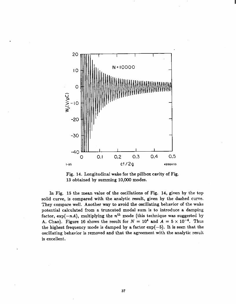
Fig. 14. Longitudinal wake for the pillbox cavity of Fig. 13 obtained by summing 10,000 modes.

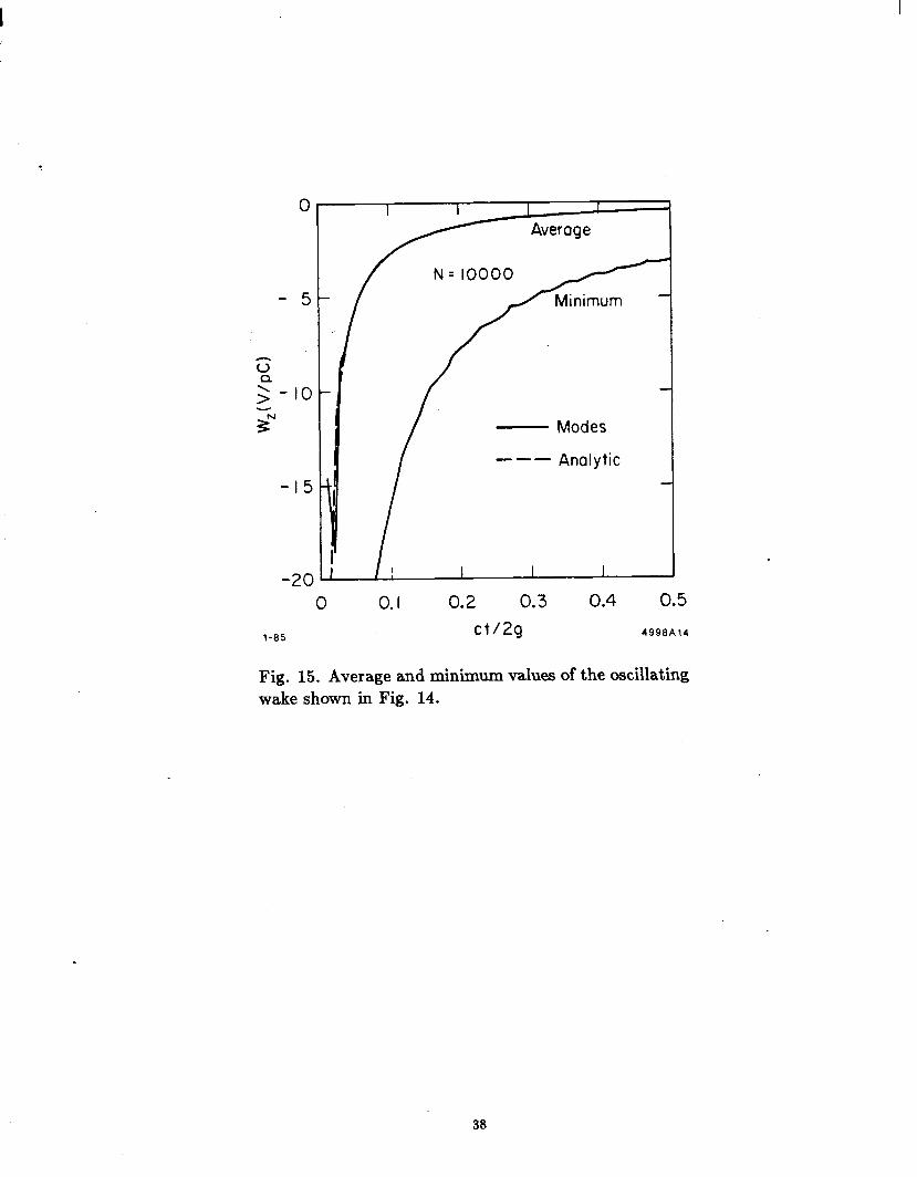
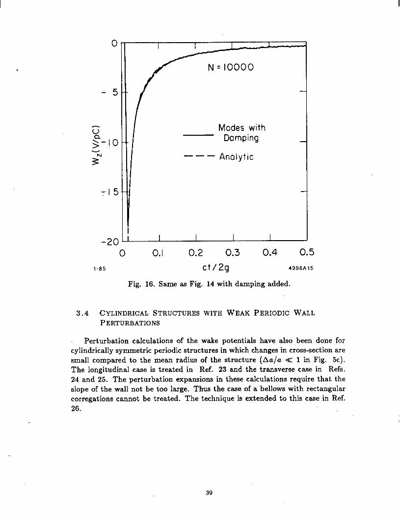
In Fig. 15 the mean value of the oscillations of Fig. 14, given by the top solid curve, is compared with the analytic result, given by the dashed curve. They compare well. Another way to avoid the oscillating behavior of the wake potential calculated from a truncated modal sum is to introduce a damping factor, exp(-nA), multiplying the rzth mode (this technique was suggested by A. Chao). Figure 16 shows the result for N = lo4 and A = 5 x 10d4. Thus the highest frequency mode is damped by a factor exp(-5). It is seen that the oscillating behavior is removed and that the agreement with the analytic result is excellent.

37

0

- 5

G a 3 -to

2

-15

-20

- -- Analytic

- Modes

0 0.1 0.2 0.3 0.4 0.5 1-85 ct/2g 4998A14

Fig. 15. Average and minimum values of the oscillating wake shown in Fig. 14.

38

0

- 5

G s-10 - r”

35

-20

Modes with Damping

- - - Analytic

0 0.1 0.2 0.3 0.4 0.5

1-85 ct/2g 4998A15

Fig. 16. Same as Fig. 14 with damping added.

3.4 CYLINDRICAL STRUCTURES WITH WEAK PERIODIC WALL PERTURBATIONS

Perturbation calculations of the wake potentials have also been done for cylindrically symmetric periodic structures in which changes in cross-section are small compared to the mean radius of the structure (Au/a < 1 in Fig. SC). The longitudinal case is treated in Ref. 23 and the transverse case in Refs. 24 and 25. The perturbation expansions in these calculations require that the slope of the wall not be too large. Thus the case of a bellows with rectangular corregations cannot be treated. The technique is extended to this case in Ref. 26.

39

4. WAKE POTENTIALS OF CHARGE DISTRIBUTIONS

4.1 LONGITUDINAL WAKE POTENTIAL FOR POINT CHARGES AND SHORT CHARGE DISTRIBUTIONS

In Section 2.2 it was shown that the longitudinal wake seen by a point charge is just one-half of the wake immediately behind the charge (see Eq. (2.45)). This fact has been called the fundamental theorem of beam loading. The validity of this theorem can be traced back to the assumption of causality. This can be seen directly if we imagine a bunch so short that the delta-function wake is essentially constant over the length of the bunch. Following a proof by Chao,[“’ we can write the energy loss for an arbitrary longitudinal current distribution I(t) as

AU = /m dt I(t) V(t) = /m dt I(t) ] do I(T) W& - T) . (4.1) -W -W -w

In writing this relation we also implicitly assume that both causality and super- position apply. As the bunch length approaches zero, the wake can be treated as constant, giving

AU= Wx(O+) j?dt I(t) 1 do I(T) . --co -CO

An integration by parts gives

AU= $ We(o+) ,

(4.2)

(f-3)

which by definition is equal to Q2Wz(0), giving

Wz(o+) = 2W*(O) . (4.4

This relation can be proven in the frequency domain using conservation of energy and assuming orthogonal normal modes. Let the stored energy .in a particular normal mode in a cavity be related to the voltage gained by a nonperturbing test particle by U = aV 2. Assume that a point charge Q passes through the cavity inducing a voltage vb, and that the fraction f vb of the induced voltage acts on the charge itself. Assume now that a second identical charge passes through the cavity along the same path and at such a phase that the voltage induced by the second charge exactly cancels the voltage induced by the first charge. Note that superposition has been assumed, along with the fact

4.0

that the motion of the second charge is not significantly perturbed by the fields induced by the first charge. The second charge sees an accelerating voltage vb and a decelerating voltage fvb, giving by superposition a net accelerating voltage vb(l - f). s ince there is no energy remaining in the cavity, energy lost by the first charge must be equal to the energy gained by the second, or

Qvbf =Qv,(l-f). (4.5) This can only be valid if f = l/2. For a single charge passing through the cavity, conservation of energy gives U = aVt = f Q‘Vb. If the loss parameter k is defined by U = kQ2, then Q = ik and

V2 k=qU

(4.6) vb = 2kQ .

The proof can be generalized to the interaction of a charge with the synchronous component of a traveling wave field in a periodic structure.

Consider now a point charge with an energy large compared to its rest energy, which is brought to rest by the interaction with its self-induced field in a long, initially field free, structure. If the charge has an initial energy corresponding to a voltage QVo, it will leave behind an induced voltage given by

v@) = 29 c kA cos wAs/c = 2vo “$;;; wAs’c . x

(4.7)

If the structure supports only a single mode, then V(s) = 2Vocos ws/c. Thus the wake reaches a peak accelerating voltage which is exactly twice that of the driving charge. However, a physical bunch, even a very short bunch, consists of a large number of individual point charges which are not rigidly connected. Thus the leading charge in such a physically real bunch will experience no deceleration, while the trailing charge will experience the full induced voltage, or twice the average decelerating voltage per particle (assuming a bunch length which is short compared to the wavelength of the mode in question). If the trailing charge is just brought to rest, the induced voltage will be Vo, and only one half of the energy contained in the bunch will be transferred to the induced field. The wake potential for such a short charge distribution extending from t = 0 to t = T interacting with a single mode is illustrated in Fig. 17a. Note that within the bunch the potential is given by

v(t) = -5 / d7 1(T) , (4.8) 0

where Vi = 2kQ. The wake rings behind the bunch as - cos w(t - 6), where

41

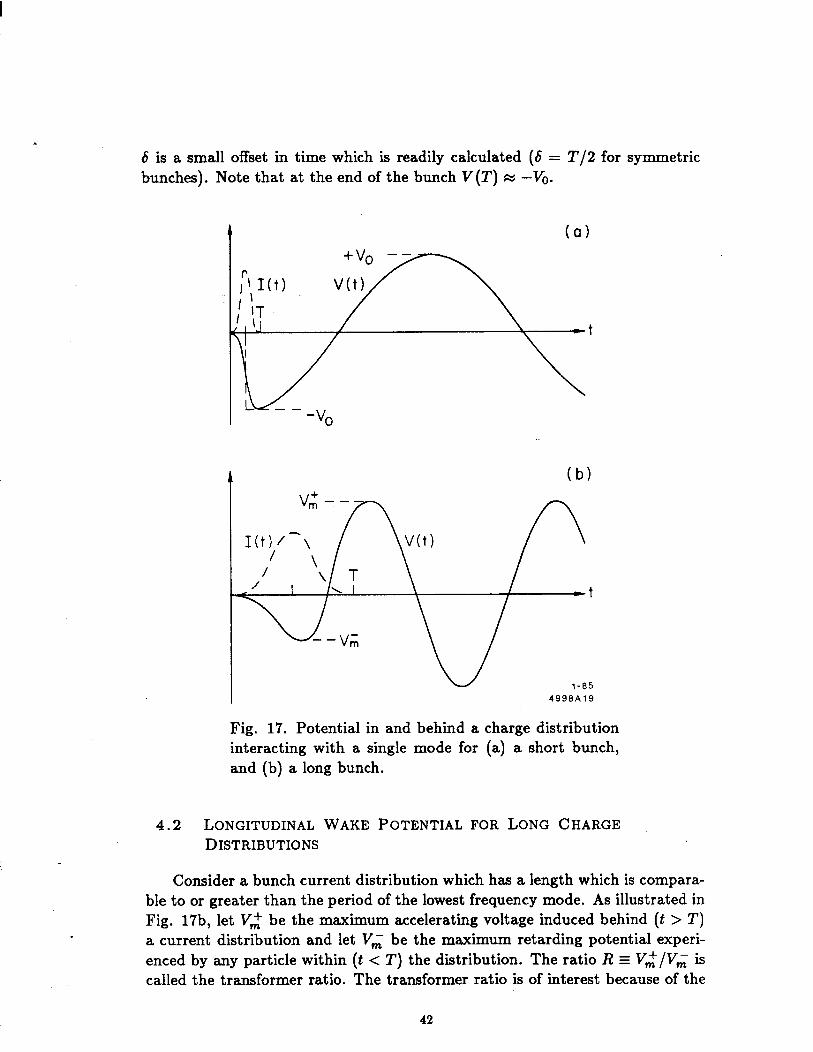
6 is a small offset in time which is readily calculated (6 = T/2 for symmetric bunches). Note that at the end of the bunch V(T) fi: -Vi.

(a)

I 499BA19

Fig. 17. Potential in and behind a charge distribution interacting with a single mode for (a) a short bunch, and (b) a long bunch.

4.2 LONGITUDINAL WAKE POTENTIAL FOR LONG CHARGE DISTRIBUTIONS

.

Consider a bunch current distribution which has a length which is compara- ble to or greater than the period of the lowest frequency mode. As illustrated in Fig. 17b, let Vm be the maximum accelerating voltage induced behind (I! > T) a current distribution and let Vi be the maximum retarding potential experi- enced by any particle within (t < 2’) the distribution. The ratio R E Vz/V& is called the transformer ratio. The transformer ratio is of interest because of the

42

possibility of wake field acceleration. If a driving bunch with particles of energy eVo is used to excite induced fields in a structure, and if V; is set equal to VO so as just to bring to rest the particles experiencing the maximum retarding potential, then the maximum accelerating potential behind the bunch is RVo. In the previous section it was shown that the transformer ratio for a short bunch interacting with a single mode is equal to one. If we consider the superposition of wake potentials for many modes, the transformer ratio for a short bunch will tend to be less than one. Since all the wake potentials are cosine like, the re- tarding wakes will tend to add coherently (in phase) within the bunch up to some maximum frequency such that w,,cr M 1. However, the wake potential for all the modes will tend to add incoherently at the first accelerating maximum behind the bunch.

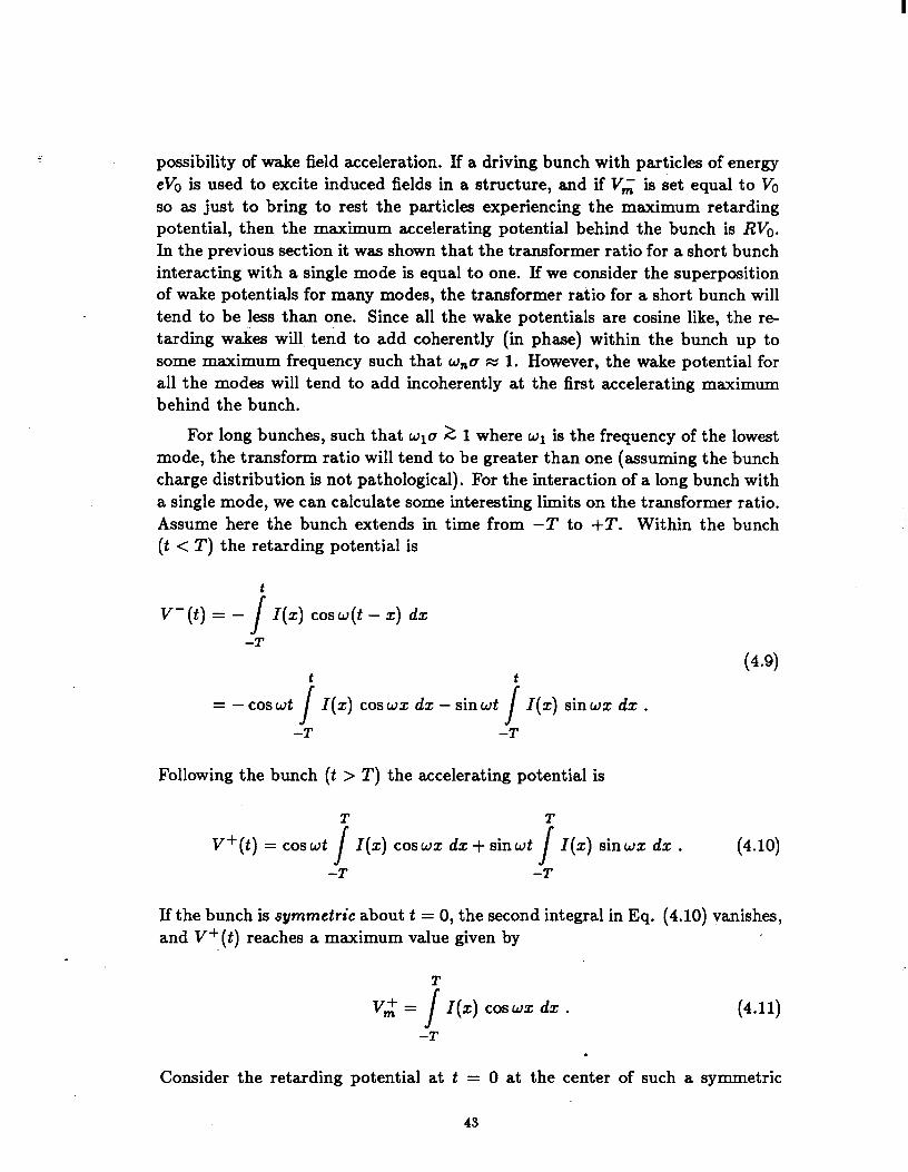
For long bunches, such that W~CT 2 1 where wr is the frequency of the lowest mode, the transform ratio will tend to be greater than one (assuming the bunch charge distribution is not pathological). For the interaction of a long bunch with a single mode, we can calculate some interesting limits on the transformer ratio. Assume here the bunch extends in time from -2’ to +T. Within the bunch (t < 2’) the retarding potential is

t

V-(t) = - /

I(x) cos w(t - x) dx -T

t t

= - cos wt /

I(x) cos wx dx - sin wt /

I(x) sin wx dx . -T -T

Following the bunch (t > 2’) the accelerating potential is

T T

v+(t) = cos wt /

I(x) cos wx dx + sin wt /

I(x) sin wx dx . (4.10) -T -T

If the bunch is symmetric about t = 0, the second integral in Eq. (4.10) vanishes, and V+ (t) reaches a maximum value given by

T

v,+ = /

I(x) cos wx dx .

-T .

(4.11)

Consider the retarding potential at t = 0 at the center of such a symmetric

43

bunch, given by

V-(O) = - ’ I(x) coswx dx = -; V; . /

-T

(4.12)

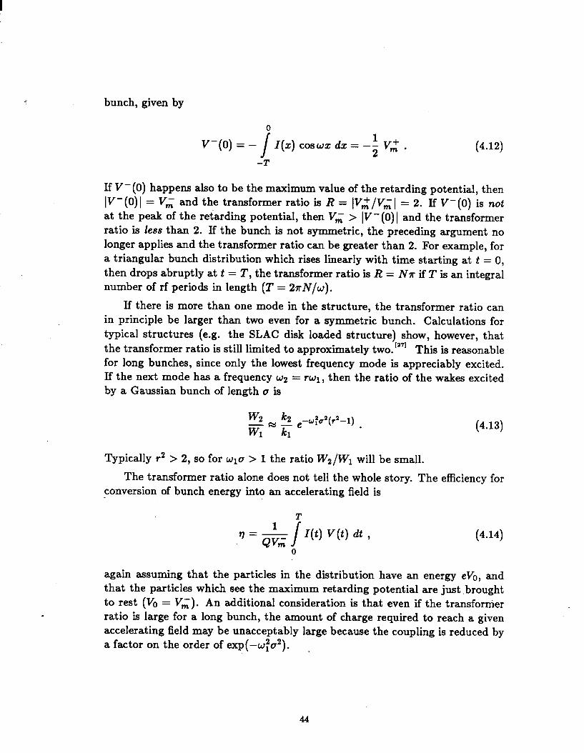
If V-(O) happens also to be the maximum value of the retarding potential, then IV-(O)I = Vi and the transformer ratio is R = IVz/V&I = 2. If V-(O) is not at the peak of the retarding potential, then V& > IV-(O)/ and the transformer ratio is less than 2. If the bunch is not symmetric, the preceding argument no longer applies and the transformer ratio can be greater than 2. For example, for a triangular bunch distribution which rises linearly with time starting at t = 0, then drops abruptly at t = T, the transformer ratio is R = NT if T is an integral number of rf periods in length (T = 27rN/w).

If there is more than one mode in the structure, the transformer ratio can in principle be larger than two even for a symmetric bunch. Calculations for typical structures (e.g. the SLAC disk loaded structure) show, however, that the transformer ratio is still limited to approximately two.‘a’l This is reasonable for long bunches, since only the lowest frequency mode is appreciably excited. If the next mode has a frequency w2 = rwl, then the ratio of the wakes excited by a Gaussian bunch of length u is

W2 h -44r2--l) -Fzr-e WI h

. (4.13)

Typically r2 > 2, so for w10 > 1 the ratio W2/Wl will be small.

The transformer ratio alone does not tell the whole story. The efficiency for conversion of bunch energy into an accelerating field is

(4.14)

again assuming that the particles in the distribution have an energy eVi, and that the particles which see the maximum retarding potential are just ,brought to rest (VO = V;). An additional consideration is that even if the transformer ratio is large for a long bunch, the amount of charge required to reach a given accelerating field may be unacceptably large because the coupling is reduced by a factor on the order of exp(-wfa2). .

44

5. WAKE FIELD ACCELERATION

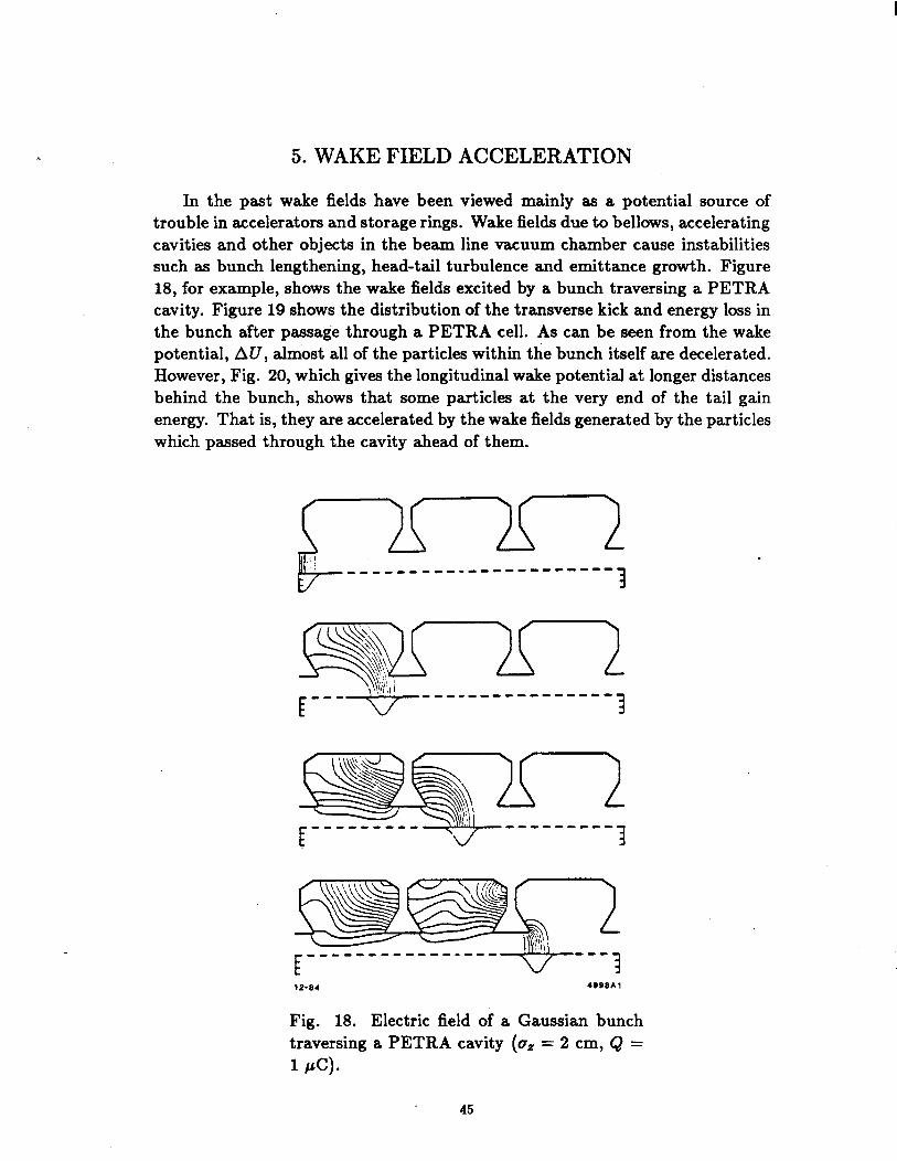
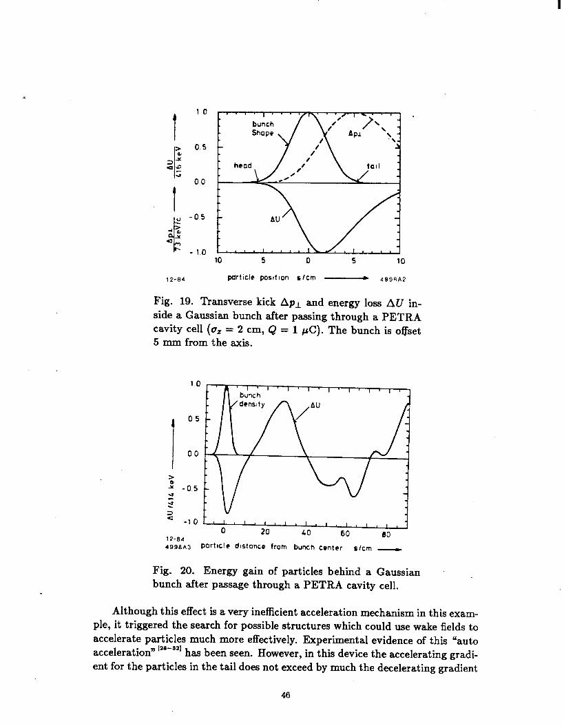
In the past wake fields have been viewed mainly as a potential source of trouble in accelerators and storage rings. Wake fields due to bellows, accelerating cavities and other objects in the beam line vacuum chamber cause instabilities such as bunch lengthening, head-tail turbulence and emittance growth. Figure 18, for example, shows the wake fields excited by a bunch traversing a PETRA cavity. Figure 19 shows the distribution of the transverse kick and energy loss in the bunch after passage through a PETRA cell. As can be seen from the wake potential, AU, almost all of the particles within the bunch itself are decelerated. However, Fig. 20, which gives the longitudinal wake potential at longer distances behind the bunch, shows that some particles at the very end of the tail gain energy. That is, they are accelerated by the wake fields generated by the particles which passed through the cavity ahead of them.

@@(--x7!

~ ___ + ---w------------ ]

Fig. 18. Electric field of a Gaussian bunch traversing a PETRA cavity (a, = 2 cm, Q = 1 PC).

45

12-94 particle pocttlon s/cm - 499RA2

Fig. 19. Transverse kick Apl and energy loss AU in- side a Gaussian bunch after passing through a PETRA cavity cell (a, = 2 cm, Q = 1 PC). The bunch is ogset 5 mm from the axis.

3 a -1 0

12-84

. tl I4d.,,,,,,,.,,,,j

0 20 LO 60 60

4998A3 POrtiCle dlstonce from bunch center s/cm

Fig. 20. Energy gain of particles behind a Gaussian bunch after passage through a PETRA cavity cell.

Although this effect is a very inefficient acceleration mechanism in this exam- ple, it triggered the search for possible structures which could use wake fields to accelerate particles much more effectively. Experimental evidence of this “auto acceleration n ‘2e-821 has been seen. However, in this device the accelerating gradi- ent for the particles in the tail does not exceed by much the decelerating gradient

46

for the majority of the particles in the center of the bunch. This follows from the general properties of the wake potential for symmetric bunches as discussed in section 4.2. By choosing the proper geometry for the structure generating the wake field, one can achieve an accelerating gradient which is up to twice the decelerating gradient within a Gaussian bunch (314 standard deviations). For practical applications this means that a few of the particles inside a 50 GeV (for example) beam could be accelerated to 150 GeV within a relatively short distance, while most of the 50 GeV particles are brought nearly to rest. Assum- ing a conventional accelerating gradient of 20 MV/m and a peak wake potential loss in a suitable down-stream structure of 50 MV/m, then the average gradient of such a system (preaccelerator + wake field section) is only about twice the gradient of the preaccelerator. Apart from this relatively modest increase in the net gradient, it is very difficult to achieve such a high longitudinal wake poten- tial without suffering the ill effect of the deflecting wake, which will also be very high. So far such wake field acceleration schemes have been studied taking only longitudinal wakes into account. ‘ss’3r1

12-84 499BA4

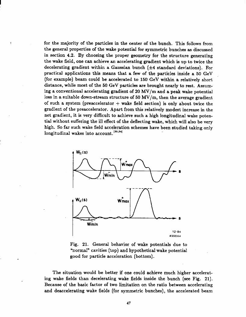
Fig. 21. General behavior of wake potentials due to “normal” cavities (top) and hypothetical wake potential good for particle acceleration (bottom).

The situation would be better if one could achieve much higher accelerat- ing wake fields than decelerating wake fields inside the bunch (see Fig. 21). Because of the basic factor of two limitation on the ratio between accelerating and deaccelerating wake fields (for symmetric bunches), the accelerated beam

47

cannot pass through the structure at the same location as the beam which gen- erates the wake field. Thus we must have two beams, an accelerated beam and a driving beam, each traversing a “wake field transformer n ‘ss~ss~ along a different path. The trick in such a wake field transformer works as follows: wake fields are generated by a driving bunch of electrons with a large number of particles at relatively low energy, passing through a particular region of the transformer. These fields are then spatially focused into a smaller region. Since the total energy in the field is conserved, the field strength increases with the degree of spatial focusing. Thus-much higher fields can be produced in this second smaller region in the wake field transformer than the fields seen by the .particles in the driving beam. These fields can now be used to accelerate a second beam (of course with fewer particles) at very high gradients.

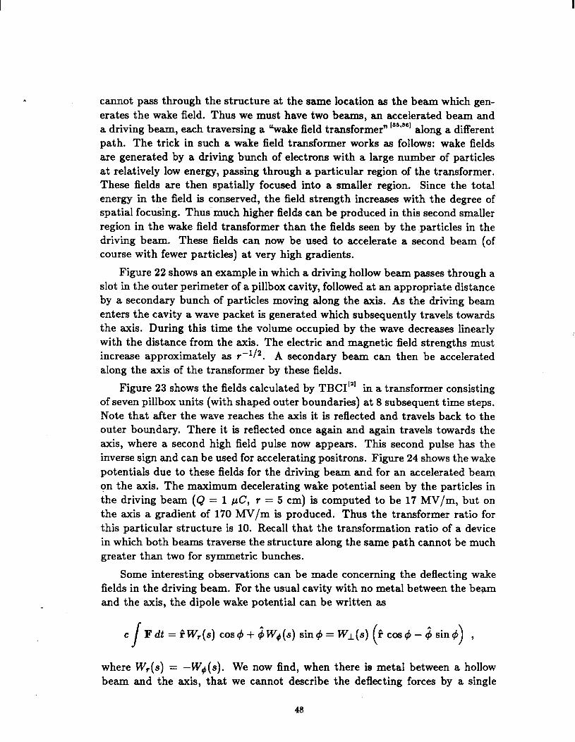
Figure 22 shows an example in which a driving hollow beam passes through a slot in the outer perimeter of a pillbox cavity, followed at an appropriate distance by a secondary bunch of particles moving along the axis. As the driving beam enters the cavity a wave packet is generated which subsequently travels towards the axis. During this time the volume occupied by the wave decreases linearly with the distance from the axis. The electric and magnetic field strengths must increase approximately as t -li2. A secondary beam can then be accelerated along the axis of the transformer by these fields.

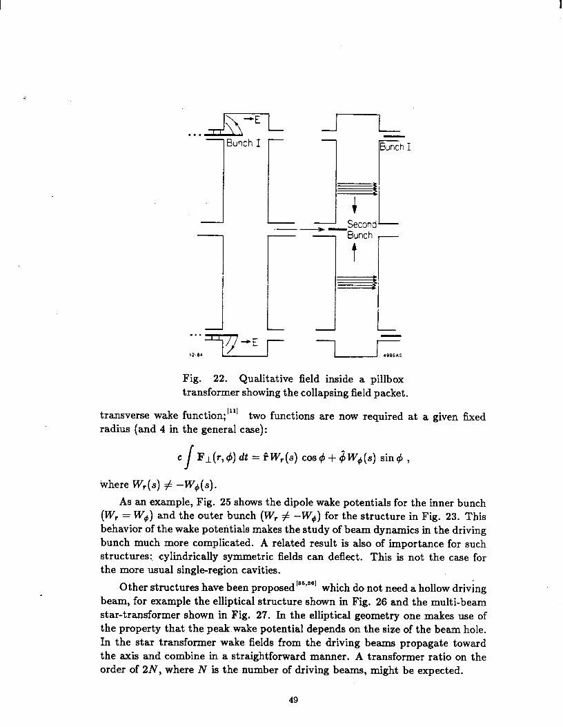
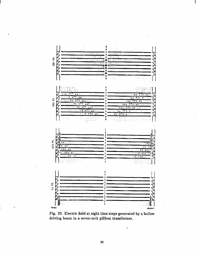
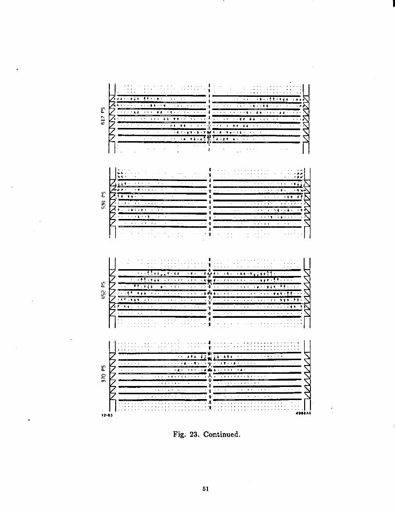
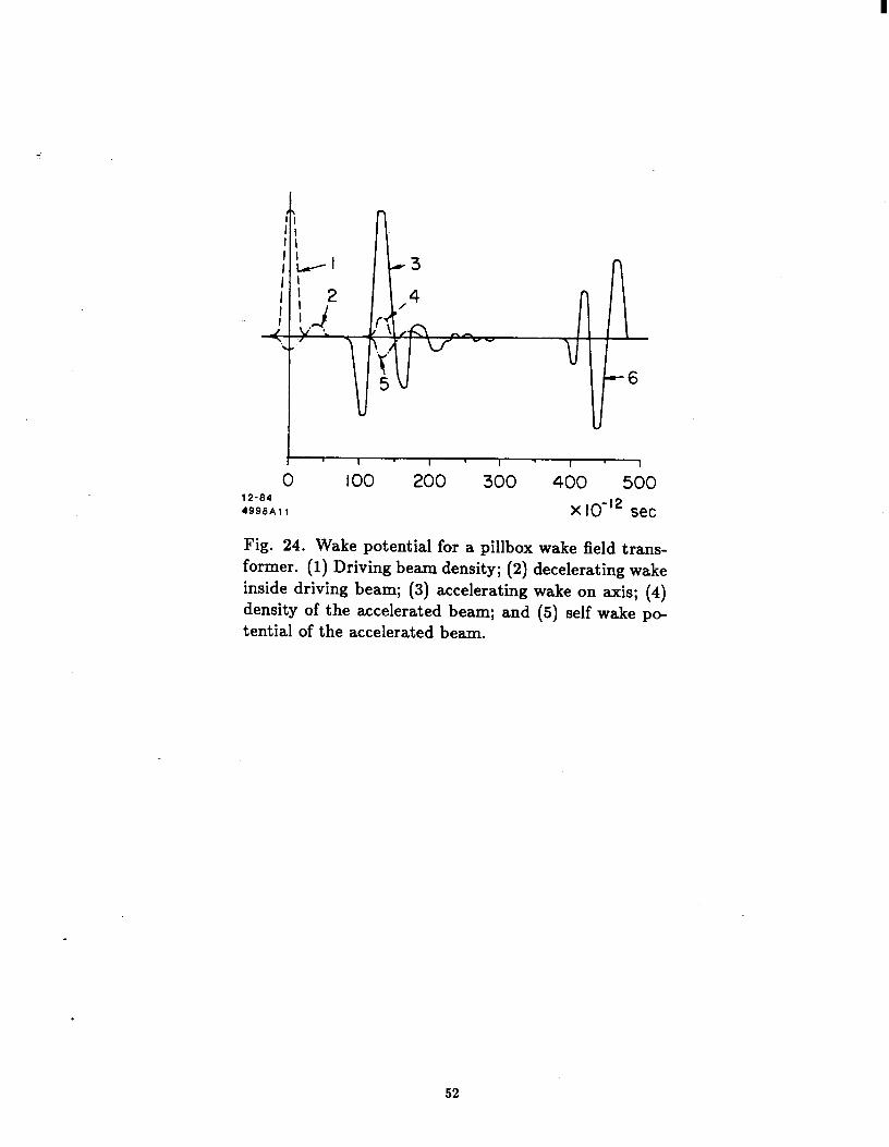
Figure 23 shows the fields calculated by TBCI”’ in a transformer consisting of seven pillbox units (with shaped outer boundaries) at 8 subsequent time steps. Note that after the wave reaches the axis it is reflected and travels back to the outer boundary. There it is reflected once again and again travels towards the axis, where a second high field pulse now appears. This second pulse has the inverse sign and can be used for accelerating positrons. Figure 24 shows the wake potentials due to these fields for the driving beam and for an accelerated beam on the axis. The maximum decelerating wake potential seen by the particles in the driving beam (Q = 1 PC, r = 5 cm) is computed to be 17 MV/m, but on the axis a gradient of 170 MV/ m is produced. Thus the transformer ratio for this particular structure is 10. Recall that the transformation ratio of a device in which both beams traverse the structure along the same path cannot be much greater than two for symmetric bunches.

Some interesting observations can be made concerning the deflecting wake fields in the driving beam. For the usual cavity with no metal between the beam and the axis, the dipole wake potential can be written as

c I

Fdt =SV,(s) COSC$+&~$( ) s sin4=Wl(s) (PcosO-Jsin4) ,

where W,(s) = -Wd(s). W e now find, when there is metal between a hollow beam and the axis, that we cannot describe the deflecting forces by a single

48

. ..m Bunch I

1 !

Fig. 22. Qualitative field inside a pillbox transformer showing the collapsing field packet.

transverse wake function;‘“’ two functions are now required at a given fixed radius (and 4 in the general case):

c /

Fl(r,r$) dt = ?Wr(s) COSC#J + c$VV~(S) sin4 ,

iivhere W,(S) # -W#(s).

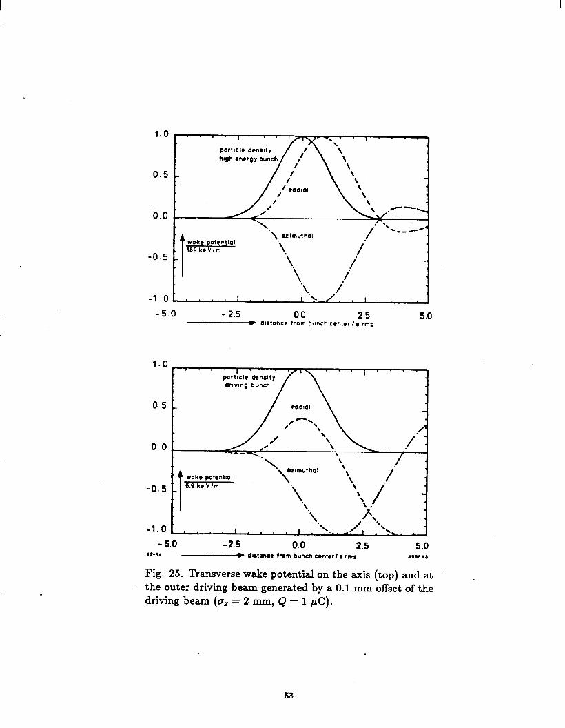
As an example, Fig. 25 shows the dipole wake potentials for the inner bunch (IV, = IV+) and th e outer bunch (IV, # -W4) for the structure in Fig. 23. This behavior of the wake potentials makes the study of beam dynamics in the driving bunch much more complicated. A related result is also of importance for such structures:. cylindrically symmetric fields can deflect. This is not the case for the more usual single-region cavities.

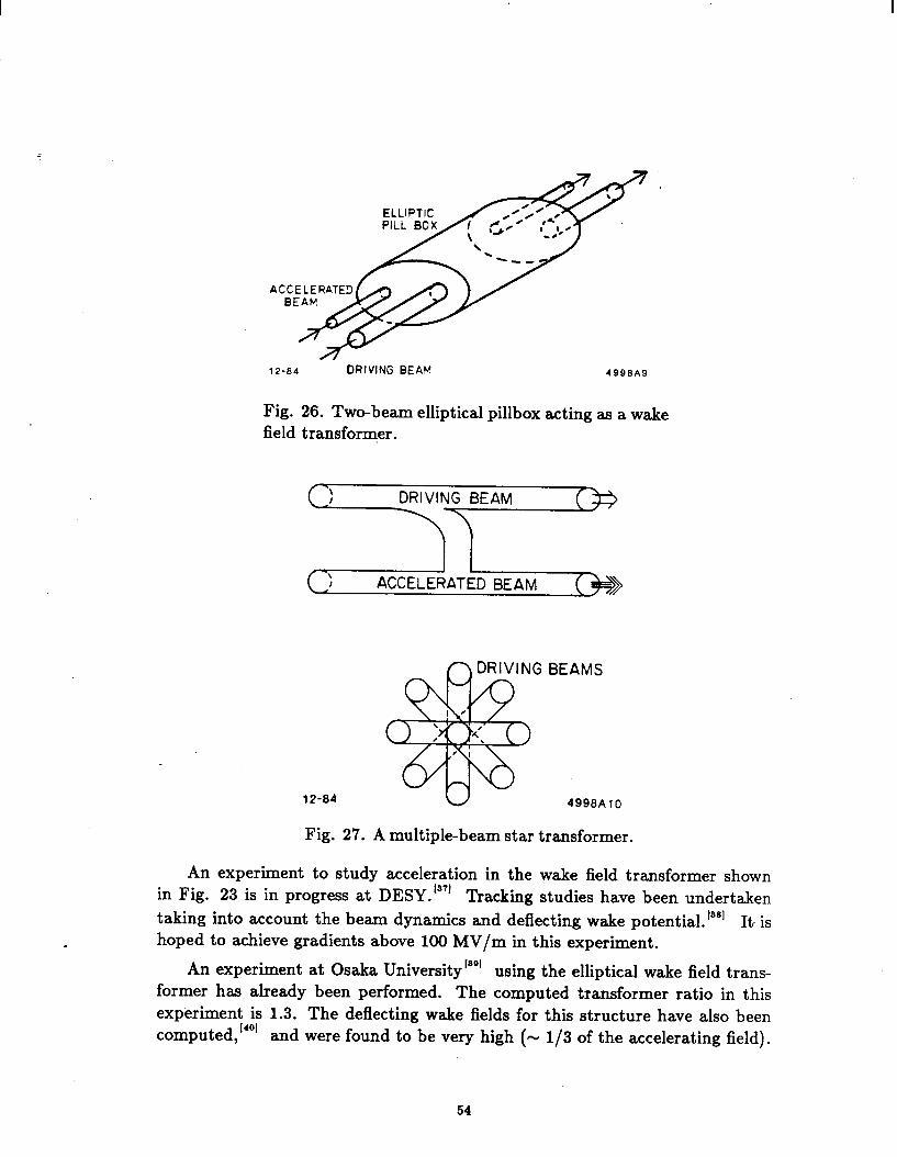
Other structures have been proposed’a”S6’ which do not need a hollow driving beam, for example the elliptical structure shown in Fig. 26 and the multi-beam star-transformer shown in Fig. 27. In the elliptical geometry one makes use of the property that the peak wake potential depends on the size of the beam hole. In the star transformer wake fields from the driving beams propagate toward the axis and combine in a straightforward manner. A transformer ratio on the order of 2N, where N is the number of driving beams, might be expected.

49

I I .: I .,,,,I. I I I1 ,I....

.I(.((,. 2

;(; v .,.. #,.1(**t.t1...

it

IF?-

‘I’ , . , ( .,I.., I 9 I 8 IE , I I .,, “‘I”“’ I tn..,*, .I, I b I I

I I ‘3’ “Y I I

I I-::.::;;::: I . , , I ., .;;:::::I I .\. ,,, II

I&- ,,,r*.+ TT.,* 1 . ...!. , tJ7 ‘:

.I ,,I .,.

lr:.t' I. ..i%

e .. %‘a-,* ct:.((,. w ‘.- rt.c+f ((1

. . .I .I,

tr’ -F--

rt*ry: liv . .I ,. Its. 44t

s,a*e,?tl~4#

i I I I I I I I I .

, ‘1

I I ,..,.. . . . . . . . . . . . ,... ; .:;;::‘:.::‘:..... . . . . I I

a.., . . , . . G.. . . . . . . .

. . . . . .

1244 4908A7

Fig. 23. Electric field at eight time steps generated by a hollow driving beam in a seven-unit pillbox transformer.

.

50

I

4 ” . ..‘. 1

.,, 1, ,( , IS.,,.,, ( .I. (( 1, II. .I . . ,,ri~jr,,,r~,,4~t,~I(.,., * , ‘4.1)14,

r ifbl+* A’ a* 8

.

_. -I .e .‘. .\x

;, :/ ::::::y.. :,. ;;; I

d- m;( ',,, I,. 1

I -'I

: . , (, ',' rfl, I %,$.,I. , , , * , 9 ..* ,t, .,I *, I . . 1lV 4f . 1 . ..!I 4, ..I,

5-

,...,.,(,. I,.,,.., 9 I ,(I,(,., I. -I - I ,~IlClll 3. ?I

,I ..,,,,, ‘T’ ,

I. II ,,

\ - -__

I .

I *.,*I,,'.*..', .I ,,I.,, II ., .I

,.. ., : : 8

. , ..:: .

. . :,~.,.:. .: .:.:...::.:..

............ ..... .. . ....... ................. ........ ..... .... ...... ........... _. ....... ....... ., ...... ................

i;-’ .* rkr*( 2 ...............

. bAk1 ....... ..... , , . l,,.l,,!,.,,*l*,~~.~ I I 1

5 ,~,.,,,~I4JL,,.,,,.I,, .,

- 'I' . ,,.I,,.,,* ,,,,.,,..,,.I,,... -?I ‘1.

- : l. _

t

I , . . , , . * .

, , . . , . . . .‘.I” , . a, .a.

, . . . . , . * , I

- 1.Y . . .

. . . . . .(. . . . . . . . : : :

_. . . . . . . . .__., . . . ._. . . . .__.._. ._. . . . . . . . . . . . . . . . . . 1 _^--.r

12-83 .““e)AD

Fig. 23. Continued.

51

0 12-84 4998A 11

too 200 300 400 500 X IO-l2 set

Fig. 24. Wake potential for a pillbox wake field trans- former. (1) Driving beam density; (2) decelerating wake inside driving beam; (3) accelerating wake on axis; (4) density of the accelerated beam; and (5) self wake po- tential of the accelerated beam.

pottlcle density

woke potentlot 16.9 keVlm

‘\. \ ozimuthol

-5.0 - 2.5 0.0 2.5 5.0 ___C dlstonce from bunch center I e rmg

0.5 - 0.5 - L J

/ / \ \

\

0.0 ,’ ./’ : 0.0

woke potent101 woke potent101

-0.5 -0.5

j j

6.9 6.9 Lo V/m Lo V/m

-1.0 -1.0 *‘I * I I ,

- 5.0 -2.5 0.0 2.5 12-04 M dtstmce from bunch center/ l rms

- 5.0 -2.5 0.0 2.5 5.0 12-04 M dtstmce from bunch center/ l rms 4998A8

Fig. 25. Transverse wake potential on the axis (top) and at the outer driving beam generated by a 0.1 mm offset of the driving beam (a, = 2 mm, Q = 1 @ I!).

53

12-84 DRIVING BEAM 4998A9

Fig. 26. Two-beam elliptical pillbox acting as a wake field transformer.

12-84

BEAMS

4998A 10

Fig. 27. A multiple-beam star transformer.

An experiment to study acceleration in the wake field transformer shown in Fig. 23 is in progress at DESY.“” Tracking studies have been undertaken taking into account the beam dynamics and deflecting wake potential. w It- is hoped to achieve gradients above 100 MV/m in this experiment.

An experiment at Osaka University’Sg1 using the elliptical wake field trans- former has already been performed. The computed transformer ratio in this experiment is 1.3. The deflecting wake fields for this structure have also been computed,“” and were found to be very high (- l/3 of the accelerating field).

54

ACKNOWLEDGEMENTS

The authors would like to thank R. K. Cooper for reading the manuscript and providing helpful suggestions. Thanks are due also to P. L. Morton for his comments and insights, particularly concerning the physics of resistive wall wake fields.

REFERENCES

0 T. Weiland, DESY 82-015 (1982) and NIM 212, 13 (1983). L.

3.

4.

E.U. Condon, J. Appl. Phys.12, 129 (1941).

P. Morton and K. Neil, UCRL-18103, Lawrence Radiation Laboratory, Berkeley, Calif. (1968); p. 365.

P. Morse and H. Feshbach, Methods of Theoretical Physics (McGraw-Hill, New York, 1953), p. 1769.

1. R.F. Koontz, G.A. Loew, R.H. Miller, P.B. Wilson, IEEE Trans. Nucl. Sci. NS-24, 1493 (1977).

5.

6.

7.

8.

9.

10.

- 11.

12.

13.

14.

15.

16.

17.

18. .

K. Bane, CERN/ISR-TH/80-47 (1980).

W .K.H. Panofsky and W.A.Wenzel, Rev. Sci. Instrum. 27, 967(1956).

D. Watkins,Topics in Electromagnetic Theory, (John Wiley and Sons, New York, 1958), Sec. 1.2.

A. Akhiezer, I. Fainberg and G. Liubarski, J. Tech. Phys. USSR 25, 2526 (1955).

K. Bane and B. Zotter, Proceedings of the llth Int. Conf. on High Energy Accelerators, CERN (Birkhguser Verlag, Basel, 1980), p. 581.

T. Weiland, DESY M83-02 (1983) and NIM 216, 31 (1983).

K. Bane and P. Wilson, Proceedings of the llth Int . Conf. on High-Energy Accelerators, CERN (Birkhguser Verlag, Basel, 1980), p. 592.

E. Keil, Nucl. Instrum. Methods 100, 419 (1972).

D. Brandt and B. Zotter, CERN-ISR/TH/82-13 and LEP Note 388 (1982).

K. Bane and T. Weiland, SLAC/AP-1 (1983).

R.V. Churchill, Fourier Series and Boundary Value Problems (McGraw- Hill, New York, 1941); Sec. 52.

P.L. Morton, V.K. Neil and A.M. Sessler, J. Appl. Phys. 37, 3875 (1966).

A.W. Chao in Physics of High Energy Particle Accelerators, AIP Conf. Proc. No. 105, (Am. Inst. of Physics, New York, 1983), Sets. 1.2 and 1.3.

55

19. P. Morton and P. Wilson, Internal note AATF/79/15, SLAC (1979).

20. T. Weiland and B. Zotter, Particle Accelerators 11, 143 (1981).

21. A. Papiemik, M. Chatard-Moulin and B. Jecko, Proceedings of the gth Int. Conf. on High Energy Accelerators, SLAC (1974), p. 375.

22. A.W. Chao and P.L. Morton, PEP-105, SLAC (1975).

23. M. Chatard-Moulin and A. Papiemik, IEEE Trans. Nucl. Sci. NS-26, 3523 (1979).

24. S. Krinsky, Proceedings of the llth Int. Conf. on High Energy Accelerators (Birkhluser Verlag, Basel, 1980), p. 576.

25. R.K. Cooper, S. Krinsky and P.L. Morton, Particle Accel. 12, 1 (1982).

26. S. Krinsky and R.L. Gluckstem, IEEE Trans. Nucl. Sci. NS-28, 2621 (1981).

27. J. T. Seeman, IEEE Trans. Nucl. Sci. NS-30, 3180 (1983).

28. M. Friedman, Phys. Rev. Letters 31, 1107 (1973).

29. N.R. Heese and W.R. Randorf, Rev. Sci. In&r. 43, 1594 (1972).

30. I.A. Grishaev and A.M. Shenderovich, Sov. Phys. Tech. Phys. 17, 1871 (1973).

31. L.N. Kazanskii, A.V. Kisletsov, A.N. Lebedev, Atomnaya Energiya 30,27 (1971).

32. R.J. Briggs, T.I. Fessenden, V.K. Neil, Proceedings of the gth Int. Conf. on High Energy Accelerators, SLAC (1974), p. 278.

33. E.A. Perevedentsev and A.N. Skrinsky, Proc. of 6th All-Union Conf. on Charged Particle Accel., Dubna (1978), Vol. 2, p. 272.

-34. J.T. Seeman, Cornell report CBN 82-17 (1982).

35. G.A. Voss and T. Weiland, DESY M82-10 (1982).

36. G.A. Voss and T. Weiland, DESY 82-074 (1982).

37. The wake field accelerator study group, DESY M83-27 (1983) and Pro- ceedings of the 12th Jnt. Conf. on High Energy Accelerators, Fermilab, (1983), p. 454.

38. T. Weiland and F. Willeke, DESY M82-24 (1983) and Proceedings of the 12th Int. Conf. on High Energy Accelerators, Fermilab, (1983), p. 457.

39. S. Takeda, Osaka University, private communication.

40. Y. Chin, KEK 83-19 (1983).

56