SLAC - 338 UC - 34D 09 RESONANCE PRODUCTION IN C · 2006. 8. 14. · tically into a pair of charged...
117
RESONANCE PRODUCTION IN TWO-PHOTON INTERACTIONS* SLAC - 338 UC - 34D 09 Natalie Ann Roe C Stanford Linear Accelerator Center Stanford University Stanford, California 94309 February 1989 Prepared for the Department of Energy under contract number DE-AC03-76SF00515 Printed in the United States of America.- Available from the National Technical Infor- mation Service, U.S. Department of Commerce, 5285 Port Royal Road, Springfield, Virginia 22161. Price: Printed Copy A06, Microfiche AOl. * PH.D. DISSERTATION
Transcript of SLAC - 338 UC - 34D 09 RESONANCE PRODUCTION IN C · 2006. 8. 14. · tically into a pair of charged...
RESONANCE PRODUCTION IN
TWO-PHOTON INTERACTIONS*
SLAC - 338 UC - 34D
09
Natalie Ann Roe C
Stanford Linear Accelerator Center
Stanford University
Stanford, California 94309
February 1989
Prepared for the Department of Energy
under contract number DE-AC03-76SF00515
Printed in the United States of America.- Available from the National Technical Infor-
mation Service, U.S. Department of Commerce, 5285 Port Royal Road, Springfield,
Virginia 22161. Price: Printed Copy A06, Microfiche AOl.
* PH.D. DISSERTATION

ii
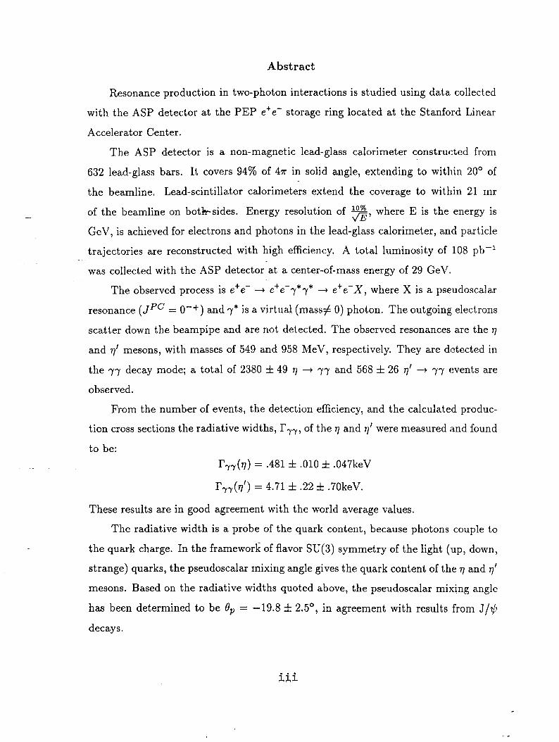
Abstract
Resonance production in two-photon interactions is studied using data collected
with the ASP detector at the PEP e+e- storage ring located at the Stanford Linear
Accelerator Center.
The ASP detector is a non-magnetic lead-glass calorimeter constructed from
632 lead-glass bars. It covers 94% of 47r in solid angle, extending to within 20” of
the beamline. Lead-scintillator calorimeters extend the coverage to within 21 mr
of the beamline on bothsides. Energy resolution of m where E is the energy is a’
GeV, is achieved for electrons and photons in the lead-glass calorimeter, and particle
trajectories are reconstructed with high efficiency. A total luminosity of 108 pb-’
was collected with the ASP detector-at a center-of-mass energy of 29 GeV.
The observed process is e+e- + e+e-y*y* + e+e-X, where X is a pseudoscalar
resonance (Jpc = O-+) and 7 * is a virtual (mass# 0) photon. The outgoing electrons
scatter down the beampipe and are not detected. The observed resonances are the 77
and 7’ mesons, with masses of 549 and 958 MeV, respectively. They are detected in
the yy decay mode; a total of 2380 f 49 77 -+ yy and 568 f-26 q’ + ry events are
observed.
From the number of events, the detection efficiency, and the calculated produc-
tion cross sections the radiative widths, I’,,,,, of the 77 and 7’ were measured and found
to be:
I’,-,(q) = .481 f .OlO & .047keV
lYrr(q’) = 4.71 f .22 f .7OkeV.
These results are in good agreement with the world average values.
The radiative width is a probe of the quark content, because photons couple to
the quark charge. In the framework of flavor SU(3) symmetry of the light (up, down,
strange) quarks, the pseudoscalar mixing angle gives the quark content of the 77 and 7’
mesons. Based on the radiative widths quoted above, the pseudoscalar mixing angle
has been determined to be Op = -19.8 f 2.5’, in agreement with results from J/$
decays.

Acknowledgments
I would like to take this opportunity to say a word of thanks. First, to my advisor
David Burke, for his advice and support, his boundless energy, and his enthusiasm
for physics.
-
Many thanks are also due to the members of the ASP collaboration, who.made
this experiment the success it has been and who have been a pleasure to work with.
In particular, I acknowledge the camaraderie of my office-mate, Chris Hawkins, who
was a ready source of FoAtran wit and wisdom. T*om Steele’s valuable friendship and
7&X-pertise smoothed the waters and made the journey much more pleasant. Thanks
also to Lydia Beers, who brightened the way with humor and a friendly smile.
Finally, I want to thank my mother for weekly doses of encouragement, my
father and brothers for keeping my Alfa Romeo running, and my husband Michael
for everything else.
,
iv
Contents
Abstract
Acknowledgments
List of tables L - List of figures
1 Introduction to Two-Photon Interactions
1.1 Historical Development
1.2 The Equivalent Photon Approximation
1.3 Properties of Two-Photon Interactions
1.4 Exact Lowest-Order Calculations
1.5 The Pseudoscalar Resonances and SU(3) Symmetry
2 Experimental Apparatus
2.1 The ASP Detector
2.2 Online Calibration and Monitoring
2.3 The Trigger
3 Event Reconstruction
3.1 Off-line Calibration
3.2 Energy Determination
3.3 Tracking
4 Event Simulation
4.1 Event Generation
4.2 Detector Simulation
4.3 Trigger Simulation
5 Event Selection
5.1 Production First Pass
5.2 Analysis First Pass
. . . 111
iv
Vii
viii,
1
4
6
7
10
13
16
17
23
25
30
30
32
35
39
40
41
45
48
48
49

5.3 Final Event Selection
6 Background Calculations
6.1 Sources of Background Events
G.2 Fourth-Order QED Backgrounds
6.3 Two-photon backgrounds
6.4 Cosmic Rays
6.5 Beam-Gas Interactions
- 6.6 Summary of Background Contributions
7 Efficiency Calculazons
7.1 Detector Acceptance
- 7.2 Trigger Efficiency
7.3 Production First Pass Efficiency
7.4 Analysis First Pass Efficiency
7.5 Final Event Selection Efficiency
7.6 Luminosity Measurement
8 Results and Conclusions
8.1 Fitting the 77 Invariant Mass Distribution
8.2 The Radiative Widths of the q and 7’.
8.3 The Pseudoscalar Mixing Angle
8.4 Summary and Conclusions
Appendix A Forward Drift Chambers
A.1 Mechanical Construction
A.2 Operation and Electronic Read-Out
A.3 Performance
REFERENCES
53
57
57
57
60
63
64
68
70
71
74
78
79
80
85
88
88
91
95
98
99
100
101
102
104
vi
Tables
is 1.2
1.3 -
1.4
2.1
4;l
6.1
7.1
7.2
7.3
7.4
7.5
7.6
7.7
8.1
8.2
8.3
8.4
8.5
Spin l/2 Fundamental Particles
Mediators of the Fundamental Forces.
Definition of Frequently Used Symbols
Neutral Members of tee Pseudoscalar Nonet
Trigger Definitions
Q” Dependence of Two-Photon Cross Sections
Summary of Background Contributions,
Detector acceptance for 77 and 7’ events
7 peak and width measurements
Efficiency of production first pass cuts
Eficiency of analysis first pass cuts
Efficiency of final event selection cuts
Efficiency of analysis on data and simulated radiative Bhabhas
Summary of efhciencies.
Monte Carlo fit parameters.
Fit parameters for yr invariant mass distribution.
Summary of quantities for calculation of radiative width.
Summary of measurements of the q radiative width.
Summary of measurements of the 77’ radiative width.
3
3
8
14
27
41
69
71
76
79
79
81
82
87
91
92
93
94
95
vii

Figures
1.1
1.2
1.3 - 2.1
2.2
- 2.3
2.4
2.5
3.1
3.2
3.3
3.4
4.1
4.2
5.1
5.2 .
5.3
Photon-Photon Scattering
Two-Photon Production of electron pairs
Kinematics of the Two-Photon Process
Side view of the%SP detector
Cross section of the central detector
Forward Shower Counter construction
Summing Circuit Diagram
Trigger efficiency vs. lead-glass energy.
Attenuation in the lead glass
Radiation length of the lead glass vs. 4.
Resolution in the lead glass
Resolution on Intercept
Ratio of simulated lead-glass signal to data.
Ratio of simulated central PWC signal to data.
Threshold behavior of ‘super trigger’.
Lead-Glass quadrant time.
Lead-Glass time vs. TOF time.
Lead-Glass time - TOF time.
Shower shape of photons and 7r”‘s.
pt distribution of final data sample.
5.4
5.5
5.6
5.7
6.1
6.2
6.3
Invariant mass distribution of final data sample.
Feynman diagrams for e+e- + (e+e’)yy
e f y background invariant mass
f2 (1270) background invariant mass
2
6
7
18
19
24
26
28
31
33
35
38
43
44
50
52
52
53
55
56
56
58
60
62
. . . Vlll
6.4
6.5
6.6
6.7
6.8
6.9
7.1
7.2
-- 7.3
7.4
7.5
7.6
7.7
7.8
8.1
8.2
8.3
8.4
A.1
A.2
Crystal Ball r”ro invariant mass distribution
Continuum 1r07ro background contribution
Timing distribution of identified cosmic ray events
Timing distribution of final sample.
2 distributions of q events.
Invariant mass of beam-gas events.
13 distribution for 7 events.
8 distribution for e+e- + (e+e-)e+e- events.
Raw energy distribute%, Monte Carlo vs. data, for e-pairs.
Central PWC efficiency vs. track energy.
Stray energy distribution for Monte Carlo and data.
Lead glass shower shape distributions.
Central PWC Shower shape distributions.
Angular distribution of Bhabha events.
Invariant Mass of Monte Carlo 7 events.
Invariant Mass of Monte Carlo 7’ events.
Invariant Mass of Monte Carlo fi(1270) events.
Fitted ry Invariant Mass.
Resolution of forward drift chambers.
Drift velocity vs. distance from sense wire.
63
63
65
65
67
68
72
74
77
83
85
86
86
87
89
90
90
92
103
104
:.:- /
ix
Introduction to Two-Photon Interactions
- --
_ This thesis is a study of the production of 77 and r,? mesons in photon-photon
interactions. Time-reversal invariance implies that any state produced by two photons
may also decay back into two photons, and these are in fact the reactions which have
been observed:
YY --+ ‘I ---) 77 and yy --+ v’ -+ yy.
By way of introduction, let us first briefly describe the nature of two-photon interac-
tions and the role of mesons in particle physics.
The interaction of two photons is a purely quantum effect which was first un-
derstood in the early 1930’s with the advent of Quantum Field Theory.@) Accord-
ing to the laws of classical electrodynamics, photons do not interact; instead, their
electromagnetic fields add linearly. This principle of the linear superposition of elec-
tromagnetic fields is well established in the macroscopic domain. (‘1 However at the
subatomic level there is a finite probability for two photons to scatter, either elasti-
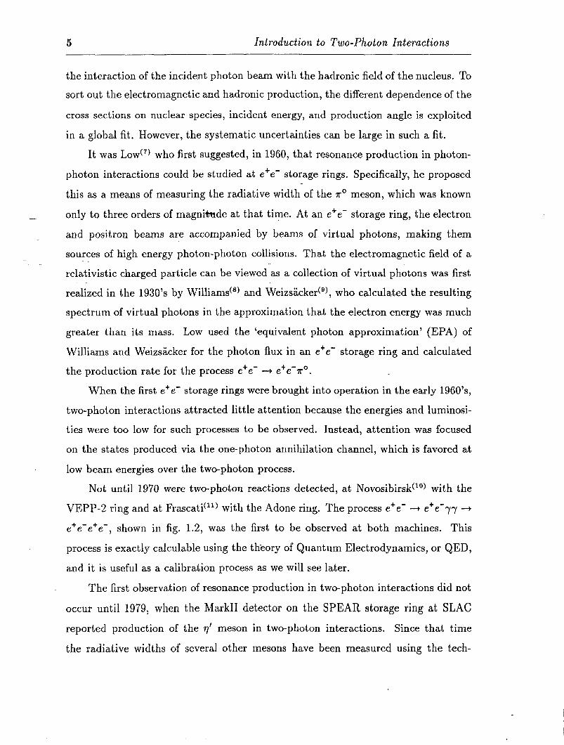
cally, into two photons, or inelastically, producing a pair of charged particles. These
processes are illustrated in the Feynman diagrams of fig. 1.1.
Because photons couple only to electric charge, they cannot couple directly to one
another. The photon self-interaction occurs by virtue of the Heisenberg uncertainty
principle, which allows a photon to become, for a short time, a pair of virtual charged
particles. This fluctuation of a photon into two charged particles is highly improbable
unless the photon has an energy greater than twice the mass of the lightest charged

1 Introduction to Two-Photon Interactions 2
Figure 1.1. The scattering of two photons, a) elastically into two photons, and b) inelas- tically into a pair of charged particles.
particle, the electron. Photons of this energy are gamma rays with a frequency greater
than 1020 cycles/set. Therefore it is not surprising that the scattering of photons by
photons is not an everyday feature ! To reach the regime where we can observe this
process we need particle accelerators where such high energies are available. The data
for this research were accumulated with the ASP detector at the PEP e+e- storage
ring (& = 29 GeV), 1 ocated at the Stanford Linear Accelerator Center.
Mesons, such as the 7 and q’, are quark anti-quark pairs, which we denote by
qq. Quarks are fundamental particles, and together with the leptons, they are the
building blocks of all matter. Quarks are the constituents of protons and neutrons,
from which atomic nuclei are made. The leptons include the familiar electron, and
its associated neutrino, which form a doublet. There are two other known lepton
doublets, or ‘generations’ of leptons. The quarks are also arranged in doublets, each
doublet consisting of one quark with +g of the electron charge and one with - 3 of the
electron charge. The three generations of leptons matches the three known generations
of quarks. (We don’t know if there is something special about the number three, or
if there are additional generations yet to be discovered.) All of the known quarks
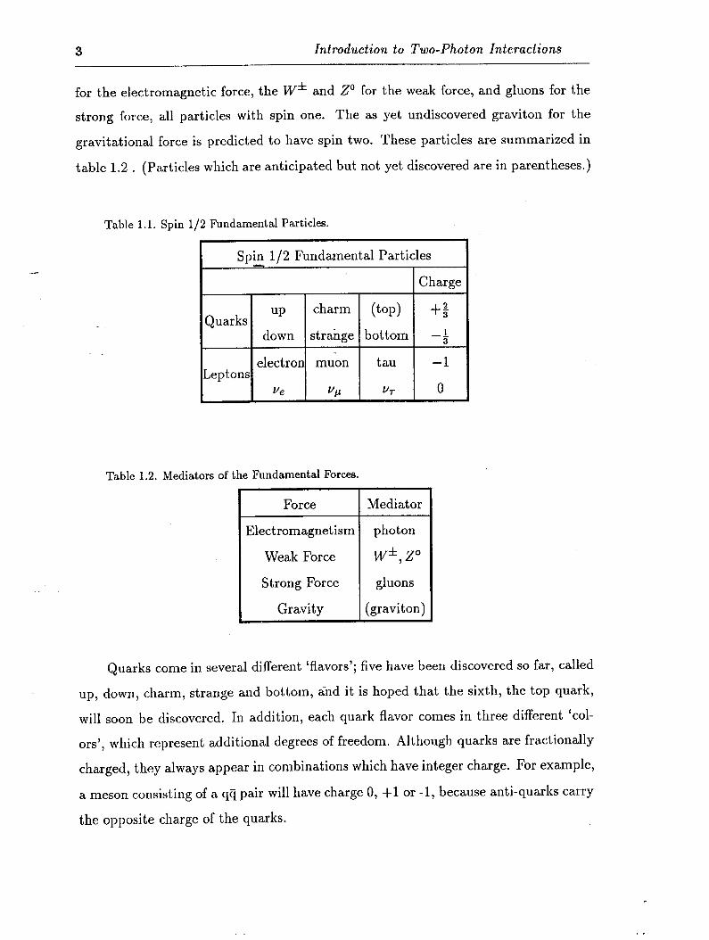
and leptons are given in table 1.1 . In addition to quarks and leptons, which are
spin l/2 fermions, the list of fundamental particles includes some integer-spin bosons
which are the mediators of the four fundamental forces. These include the photon
3 Introduction to Two-Photon Interactions
for the electromagnetic force, the W* and 2’ for the weak force, and gluons for the
strong force, all particles with spin one. The as yet undiscovered graviton for the
gravitational force is predicted to have spin two. These particles are summarized in
table 1.2 . (Particles which are anticipated but not yet discovered are in parentheses.)
Table 1.1. Spin l/2 Fundamental Particles.
I Spin l/2 Fundamental Particles .
Charge
Quarks dIzn charm (told +:
strange bottom -i
electron muon tau -1 Leptons
ve vu VT 0
Table 1.2. Mediators of the Fundamental Forces.
I Force I Mediator
Electromagnetism photon
Weak Force Wf, z”
Strong Force gluons
Gravity (graviton)
Quarks come in several different ‘flavors’; five have been discovered so far, called
up, down, charm, strange and bottom, and it is hoped that the sixth, the top quark,
will soon be discovered. In addition, each quark flavor comes in three different ‘col-
ors’, which represent additional degrees of freedom. Although quarks are fractionally
charged, they always appear in combinations which have integer charge. For example,
a meson consisting of a qq pair will have charge 0, +l or -1, because anti-quarks carry
the opposite charge of the quarks.
1.1 Historical Development 4
-
When two photons interact through the creation of virtual quark pairs, the quarks
may strongly interact in the final state to produce a qq bound state, or meson. This
process is resonant when the invariant mass of the photons is close to that of the
produced meson, greatly enhancing the rate. Any meson produced in a two-photon
interaction will, of course, be electrically neutral. The 77 and the 7’ are neutral mesons
composed primarily of the light quarks, u, d and s (for up, down and strange). In
fact, we will see later that the 77 and the 7’ can be described as linear combinations
of UU, dd, and ss quark-pairs. In this study we will measure the coupling of the 17
and q’ to two photons, which is called the radiative width, by observing the rate at
which each is produced in two-photon interactions. This will allow us to determine
how much of each quark flavor each meson contains, because the photon coupling to
quarks goes like the fourth power of the quark charge; therefore photons couple more
strongly to up quarks than to down or strange quarks.
1.1 Historical Development
The interaction of two photons was first described by Landau and Lifshitz(l)in
1934. Shortly thereafter, Euler and Kockel(3) calculated the cross section for the
elastic scattering of light by light, yy + 77, and Breit and Wheelerc4) calculated
the cross section for the inelastic scattering process yy + e+e-. Intense beams of
highly energetic photons are required to produce a measurable rate, and consequently
the observation of these processes remained experimentally unattainable for several
decades.
The first observations of photon-photon scattering employed a technique pro-
posed in 1951 by Primako@‘). An energetic photon beam was used on a nuclear
target, such as a sheet of copper or lead. The real photons in the beam interacted
with the virtual photons in the Coulombic field of the nuclei. The advantage of this
method over using two beams of photons directed at each other is the high density of
virtual photons in the target. The first measurement of the radiative width of the q
wa.s performed using this technique in 1967 by Bemporad et a1.c6). However Primakoff
production suffers from a serious experimental difficulty due to a background from
5 Introduction to Two-Photon Interactions
the interaction of the incident photon beam with the hadronic field of the nucleus. To
sort out the electromagnetic and hadronic production, the different dependence of the
cross sections on nuclear species, incident energy, and production angle is exploited
in a global fit. However, the systematic uncertainties can be large in such a fit.
It was LOW(~) who first suggested, in 1960, that resonance production in photon-
photon interactions could be studied at e+e- storage rings. Specifically, he proposed
this as a means of measuring the radiative width of the 7r” meson, which was known
- only to three orders of magnitide at that time. At an e+e- storage ring, the electron
and positron beams are accompanied by beams of virtual photons, making them
sources of high energy photon-photon collisions. That the electromagnetic field of a
relativistic charged particle can be viewed as a collection of virtual photons was first
realized in the 1930’s by Williams(s) and Weizs;icl~er(g), who calculated the resulting
spectrum of virtual photons in the approximation that the electron energy was much
greater than its mass. Low used the ‘equivalent photon approximation’ (EPA) of
Williams and Weizsacker for the photon flux in an e+e- storage ring and calculated
the production rate for the process e+e- -+ e+e-rO.
.
When the first e+e- storage rings were brought into operation in the early 1960’s,
two-photon interactions attracted little attention because the energies and luminosi-
ties were too low for such processes to be observed. Instead, attention was focused
on the states produced via the one-photon annihilation channel, which is favored at
low beam energies over the two-photon process.
Not until 1970 were two-photon reactions detected, at Novosibirsk@‘) with the
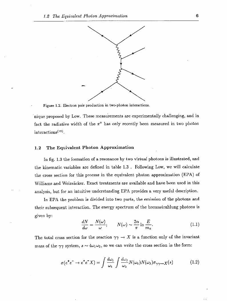
VEPP-2 ring and at Frascati(i’) with the Adone ring. The process e+e- + e+e-yy +
e+e-e+e-, shown in fig. 1.2, was the first to be observed at both machines. This
process is exactly calculable using the theory of Quantum Electrodynamics, or QED,
and it is useful as a calibration process as we will see later.
The first observation of resonance production in two-photon interactions did not
occur until 1979, when the Mark11 detector on the SPEAR storage ring at SLAC
reported production of the 77’ meson in two-photon interactions. Since that time
the radiative widths of several other mesons have been measured using the tech-
1.2 The Equivalent Photon Approximation 6
Figure 1.2. Electron pair production in two-photon interactions.
nique proposed by Low. These measurements are experimentally challenging, and in
fact the radiative width of the x0 has only recently been measured in two photon
interactions(
1.2 The Equivalent Photon Approximation
.
In fig. 1.3 the formation of a resonance by two virtual photons is illustrated, and
the kinematic variables are defined in table 1.3 . Following Low, we will calculate
the cross section for this process in the equivalent photon approximation (EPA) of
Williams and Weizsacker. Exact treatments are available and have been used in this
analysis, but for an intuitive understanding EPA provides a very useful description.
In EPA the problem is divided into two parts, the emission of the photons and
their subsequent interaction. The energy spectrum of the bremsstrahlung photons is
given by:
The total cross section for the reaction yy + X is a function only of the invariant
mass of the yr system, s N 4wi w2, so we can write the cross section in the form:
g(e+e- + e+e-X) = dwI dw,
s s - Wl
-N(WI )N(a brr-x(s) cJ2
(1.2)
‘.
I

7 Introduction to Two-Photon Interactions
Figure 1.3. Resonance production in two-photon interactions, with the notation for the variables used.
Substituting for N(w) using eq. 1.1 and keeping only the leading- terms in ln( $)
this becomes
where f is a function given by
f(x) = -(2 + x2)2 lnx - (1 - x2)(3 t x2)
(l-3)
(14
which takes on values ranging from 1 to ‘10 for most problems of interest.
1.3 Properties of Two-Photon Interactions
From eq. 1.3 several important properties of two-photon interactions can be seen
at once. First, the cross section rises logarithmically with increasing beam energy.
This is in marked contrast to annihilation into one photon, which falls like the inverse
1.3 Properties of Two-Photon Interactions 8
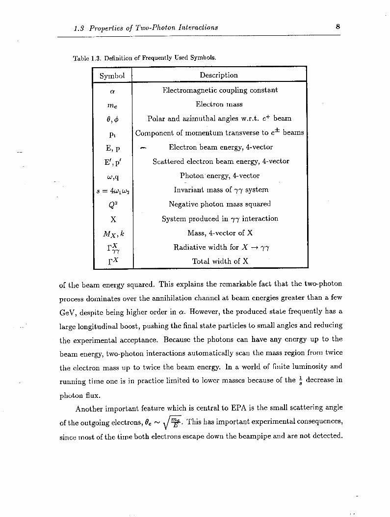
Table 1.3. Definition of Frequently Used Symbols.
Symbol Description
o! Electromagnetic coupling constant
me Electron mass
64 Polar and azimuthal angles w.r.t. e+ beam
Pt Component of momentum transverse to e* beams
E,P - Electron beam energy, 4-vector
E’ , p’ Scattered electron beam energy, 4-vector
w,q Photon energy, 4-vector
s = 4WlW2 Invariant mass of yy system
Q" Negative photon mass squared
X System produced in yy interaction
Mx,k Mass, 4-vector of X
rx 7-Y Radiative width for X + 77
rx Total width of X -
.
of the beam energy squared. This explains the remarkable fact that the two-photon
process dominates over the annihilation channel at beam energies greater than a few
GeV, despite being higher order in Q. However, the produced state frequently has a
large longitudinal boost, pushing the final state particles to small angles and reducing
the experimental acceptance. Because the photons can have any energy up to the
beam energy, two-photon interactions automatically scan the mass region from twice
the electron mass up to twice the beam energy. In a world of finite luminosity and
running time one is in practice limited to lower masses because of the 2 decrease in
photon flux.
Another important feature which is central to EPA is the small scattering angle
of the outgoing electrons, 8, N d-
y. This has import ant experiment al consequences,
since most of the time both electrons escape down the beampipe and are not detected.

9 Introduction to Two-Photon Interactions
In the ‘single-tag’ case, where the experimenter requires one of the electrons to be
detected above a minimum tagging angle, typically N lo, the cross section is reduced
by about an order of magnitude. Double-tagged experiments are down by about two
orders of magnitude in signal and consequently very few have been performed.
The small scattering angle implies a small mass for the virtual photons, defined
by:
q2 = (p’ - p)” N -2EE’(-1 - COSB’). (1.5)
- Here 8’ is the angle of the scaTtered electron and is typically very close to zero. The
virtual photons are space-like, i.e.they have a negative mass. They are often referred
to as ‘quasi-real’, being almost massless like a real photon. The variable most often
used is the positive quantity Q” = -q2. In events with high Q2, such as single- or
double-tagged events, the EPA is no longer a good approximation. In this case a form
factor should be used which incorporates the Q” dependence.
It is straightforward to identify the process e+e- -+ e*e’rr + e+e-X, even in
the untagged case. The electrons are close to the beam-line and carry little transverse
momentum. Conservation of momentum requires that the produced system X also
have low net pt. The maximum pt is given by
Pt max = 2E sine,, W-3
where 8, is the veto angle below which the electrons are undetected in the apparatus.
Because usually only one electron will be scattered at a non-zero angle, most events
will have a maximum net pt which is one-half this value. The longitudinal momentum
will usually be non-zero, so that an isotropic angular distribution in the photon-
photon center of mass will be peaked at lower angles in the lab frame. If X is
a two-particle final state, such as yr + e+e-, or decays to one as in the process
YY + 77 -+ yy, the final state particles will be back-to-back in the plane transverse
to the beam but will usually be acollinear in the plane containing the beam. This
topology, together with a low net pt and an observed energy much less than twice the
beam energy, is a very distinctive signature for two-photon interactions.
1 .d Exact Lowest-Order Calculations 10
1.4 Exact Lowest-Order Calculations
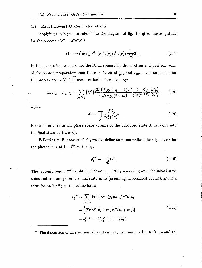
Applying the Feynman rules W) to the diagram of fig. 1.3 gives the amplitude
for the process e+e- + e’e-X:*
-
In this expression, u and u are the Dirac spinors for the electron and positron, each
of the photon propagators contributes a factor of +, and TPy is the amplitude for 4
the process 7-y 3 X. Th: cross section’is then given by:
(2n)4S(ql + q2 - k)dI’ c lM21. 1 dae+e-,,+,-X =
d3p; d3p’, P-8) spins 4dw (2n)6=12E2 ’
where
is the Lorentz invariant phase space volume of the produced state X decaying into
the final state particles kj.
Following V. Budnev et a1.(14), we can define an unnormalized density matrix for
the photon flux at the ith vertex by:
PU = -‘tP pi 2i *
Qi (1.10)
The leptonic tensor W’ is obtained from eq. 1.8 by averaging over the initial state
spins and summing over the final state spins (assuming unpolarized beams), giving a
term for each e*y vertex of the form:
tr” = C G(P: )Y’U(Pi)“(Pi)Yvu(P:) spins
(1.11)
* The discussion of this section is based on formulae presented in Refs. 14 and 16.

11 Introduction to Two-Photon Interactions
where gp” is the metric tensor defined according to the convention of Bjorken and
Drell.(15) Neglecting terms of order y we can now write the cross section in the
following form:*
due+e-.+e+e-X = (1.12)
In eq. 1.12 the photon flux factors ppV are separated from the physics of the yy + X
vertex, which is contained in tJe rank 4 tensor -
W ’ a’b’,ab = 2 s
~wfb~Mab(2~)4~(ql t qz - k)dr, (1.13)
.
This differential expression has been used to generate Monte Carlo events and to
evaluate the total cross section for two-photon production of q and 77’ mesons. The
form factor F(q,2, qi) describes how the interaction of virtual photons differs from that
of real photons, and must be determined experimentally. For events with large Q2,
the cross section is usually suppressed, i.e. F < 1, and in the limit q:, qi + 0, F + 1.
The polarization vectors c describe the helicity structure of the yr interaction,
and the indices a,b take on the values +, -, and 0. Conservation of helicity and parity
at the ry vertex implies a number of interesting properties. A detailed analysis is
given in a review by Poppe, *(16) taken together these conservation laws are known as
Yang’s theorem, (r7) which states that all states with even spin and all states with odd
spin and even parity (except J = 1) may be produced in yr interactions. This is very
different from the annihilation channel, in which the allowed quantum numbers are
limited to those of the photon, Jpc = l--. Yang’s theorem applies only in the limit
of real photons, qf,qi --j 0. If one of the photons is highly virtual any spin-parity
combination may be produced. In all cases the charge conjugation must be even.
These properties make two-photon interactions very well suited to the observation of
* In this approximation, (p,pz)’ - rnd N (ElE2 -& .ji2)’ - (2E1E2)2 = (f)2.
e2 Also, we use the convention Q = z and ti = c = 1.
1.4 Exact Lowest-Order Calculations 12
C = + resonances. In this analysis we are concerned with the neutral pseudoscalars,
which have Jpc = O-+.
The conservation laws also dictate which helicity combinations may produce a
state of given spin and parity. For pseudoscalar mesons, all combinations with one or
more longitudinal photons vanish exactly. In the untagged case, only UTT, the cross
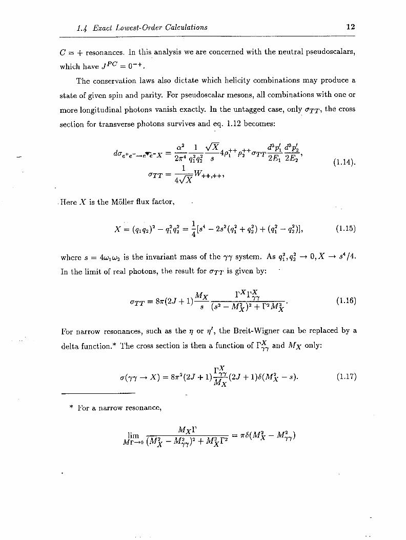
section for transverse photons survives and eq. 1.12 becomes:
.14). -
cY2 1 fi doe+e-+ewe-X = - --
d3p; d3p’, 2T4 q1”q; s W+P:+~TT~~,
1 2
- 1w,,,++,
(1.
aTT - 4&r
Here X is the Mijller flux factor,
x = (q1q2)2 - da; = ;rs4 - 2s2(qf + 4;) + (al” - a;)], (1.15)
where s = 4w1w2 is the invariant mass of the yy system. As qf , qi -+ 0, X + s4/4.
In the limit of real photons, the result for UTT is given by: -
Mx rxrx UTT = 8~(2J + l)-
s (92 - M$y: r2M$ ’ (1.16)
For narrow resonances, such as the q or $, the Breit-Wigner can be replaced by a
/ i. : : i :,
delta function.* The cross section is then a function of I’T7 and Mx only:
rx a(yy --+ X) = 87r2(2J + l)- ;; (25 + 1)6(Mg - s).
* For a narrow resonance,
= mS(Mi - M&)

13 Introduction to Two-Photon Interactions
The branching ratios of all significant decay modes have been established for the 7
and q’ mesons in fixed-target experiments, so a measurement of the production rate
in yy interactions provides a measurement not only of the radiative width but also
of the total width. This is important because the narrow total width of these states
makes them difficult to measure directly from the line shape.
To tie this discussion back into the results of section 2, we can substitute eq. 1.17
into the EPA formula (eq. 1.3) to obtain an approximation for two-photon resonance
- production given by: I)-
a(ee -+ eeX) = grf7(2J + l)(ln -$2f($$), (1.18)
where f is the function defined in eq. 1.;2. This is precisely Low’s result for 7r”
production in photon-photon interactions.
1.5 The Pseudoscalar Resonances and SU(3) Symmetry
The form of I’&,, where X is a pseudoscalar, is fixed by Lorentz and gauge
invariance to be of the form M3
where gp describes the coupling strength between two real photons and the constituent
quarks in the meson. It is interesting to note that the factor of M3 exactly cancels a
similar factor in eq. 1.18. As a result, the total two-photon production cross section
for pseudoscalars decreases rather slowly with mass according to the function f defined
in eq. 1.4.
A neutral meson can be described as a linear combination of qq pairs:
P = C ailqi@),
i
(1.20)
where the coefficients ai run over all quark flavors and are satisfy xi ai = 1.
Because photons couple to charge, it follows that g will be proportional to xi ajez,
where ei is the quark charge as given in Table 1. In the case of the light pseudoscalar

1.5 The Pseudoscalar Resonances and SU(3) Symmetry 14
mesons this coupling is described by the triangle anomaly calculation of Adler, Bell
and Jackiw,(l’) who found
sp = 1/zc\lNc 2
Tfn c ajei. (1.21) i
This is a QCD calculation in which all the non-perturbative parts are lumped together
into the pion decay constant, which has been measured in charged pion decay to be
fir = 93 MeV, and NC = 3 is the number of colors. Putting gp back into eq. 1.19,
the dependence of the rzdiative width on the fourth power of the quark charges is
evident.
The experimental determination of the coefficients ai is the goal of this analysis. - The theoretical framework is provided by the flavor symmetry of SU(3), in which the
masses of the three lightest quarks, u, d, and s, are taken to be equal. There are
3 @ 3 = 8 $1 different qq combinations which are possible, giving a nonet composed
of an octet and a singlet. There are several different nonets, one for each spin-parity
combination. The pseudoscalar nonet consists of the pions, (x+, r-, TO), the kaons
(Ii!+, K-, Ii’“, Ii;“), the 17 and the 77’. The masses, widths and branching ratios of the
neutral members of the pseudoscalar nonet are summarized in table 1.4 .
Table 1.4. Neutral members of the pseudoscalar nonet.
Resonance Mass (MeV) r
The SU(3) basis states for the neutral members of the pseudoscalar nonet are
defined by:
1~~) = +i - d;l)
I%) & = -&i+dd-ass)
1771) = +$uti + d;i + ss)
I
I (1.22) I
I / /
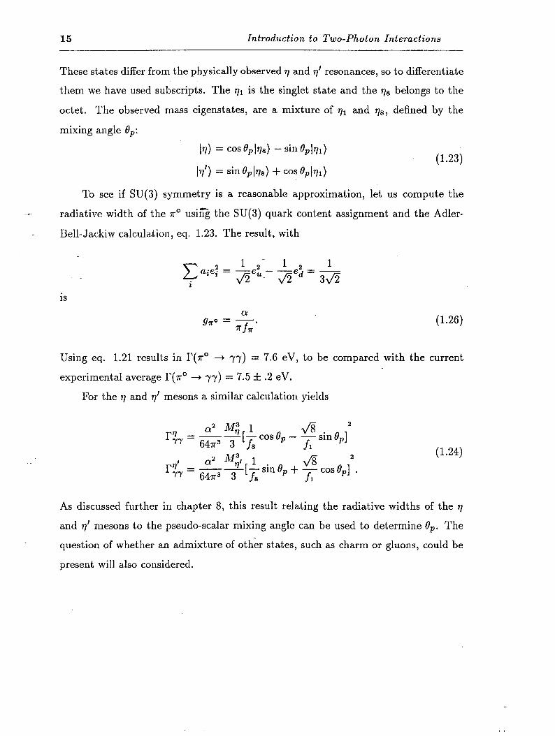
15 Introduction to Two-Photon Interactions
These states differ from the physically observed 17 and 71’ resonances, so to differentiate
them we have used subscripts. The ~1 is the singlet state and the 7s belongs to the
octet. The observed mass eigenstates, are a mixture of ql and 778, defined by the
mixing angle 0,:
I.
To see if SU(3) y s mmetry is a reasonable approximation, let us compute the
radiative width of the r” usirg the SU(3) q uark content assignment and the Adler-
Bell-Jackiw calculation, eq. 1.23. The result, with
is o!
g,o = - Tflr’
(1.26)
Using eq. 1.21 results in l?(n’ + yy) = 7.6 eV, to be compared with the current
experimental average l?(7r” 4 77) = 7.5 f .2 eV.
For the 17 and 71’ mesons a similar calculation yields
. (1.24)
As discussed further in chapter 8, this result relating the radiative widths of the r]
and 77’ mesons to the pseudo-scalar mixing angle can be used to determine I$,. The
question of whether an admixture of other states, such as charm or gluons, could be
present will also considered.
. .

2
Experimental Apparatus
The data for this experiment were collected at the Stanford Linear Accelerator
Center (SLAC) on the PEP e+e- storage ring. SLAC is a national laboratory operated
by Stanford University under contract from the U.S. Department of Energy, and is
one of three national laboratories devoted to research in particle physics in the U.S.;
the others are Fermilab, located near Chicago, Illinois, and Brookhaven National Lab,
located in Brookhaven, New York. SLAC is located on a 480-acre site adjacent to
the Stanford University campus in Palo Alto, California. SLAC has been in oper-
ation since 1964, when construction of its two-mile linear electron accelerator was
completed. This facility is the longest and most energetic linear electron accelerator
available anywhere in the world today.
The PEP collider, an e+e- storage ring with a circumference of 2.2 km, was
constructed in 1980. Electrons and positrons for PEP are supplied at an energy
of 14.5 GeV by the two-mile linear accelerator. Three electron bunches and three
positron bunches counter-rotate in the circular PEP vacuum pipe, colliding in six
interaction regions (IR’s) every 2.4~s at a total center-of-mass energy of 29 GeV. The
peak luminosity achieved at PEP was approximately 3 x 1031cm-2 set-l, and the
typical luminosity was about half that. Five of the six IR’s were occupied by large,
multi-purpose detectors. The sixth, known as IR 10, was initially uninstrumented.
In the spring of 1983 an experiment to search for weakly-interacting particles
using photon tagging was proposed to be installed in IR 10 by D. Burke and R.
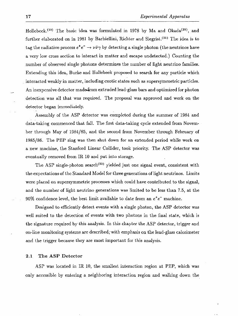
17 Experimental Apparatus
Hollebeek.(r’) The basic idea was formulated in 1978 by Ma and Okada@‘), and
further elaborated on in 1981 by Barbiellini, Richter and Siegrist.(21) The idea is to
tag the radiative process e+e- + vfiy by detecting a single photon (the neutrinos have
a very low cross section to interact in matter and escape undetected.) Counting the
number of observed single photons determines the number of light neutrino families.
Extending this idea, Burke and Hollebeek proposed to search for any particle which
interacted weakly in matter, including exotic states such as supersymmetric particles.
An inexpensive detector mad&om extruded lead-glass bars and optimized for photon
detection was all that was required. The proposal was approved and work on the
detector began immediately.
--
Assembly of the ASP detector was completed during the summer of 1984 and
data-taking commenced that fall. The first data-taking cycle extended from Novem-
ber through May of 1984/85, and the second from November through February of
1985/86. The PEP ring was then shut down for an extended period while work on
a new machine, the Stanord Linear Collider, took priority. The ASP detector was
eventually removed from IR 10 and put into storage.
The ASP single-photon search(22) yielded just one signal event, consistent with
the expectations of the Standard Model for three generations of light neutrinos. Limits
were placed on supersymmetric processes which could have contributed to the signal,
and the number of light neutrino generations was limited to be less than 7.5, at the
. 90% confidence level, the best limit available to date from an e+e- machine.
Designed to efficiently detect events with a single photon, the ASP detector was
well suited to the detection of events with two photons in the final state, which is
the signature required by this analysis. In this chapter the ASP detector, trigger and
on-line monitoring systems are described,-with emphasis on the lead-glass calorimeter
and the trigger because they are most important for this analysis.
2.1 The ASP Detector
ASP was located in IR 10, the smallest interaction region at PEP, which was
only accessible by entering a neighboring interaction region and walking down the

2.1 The ASP Detector 18
PEP arcs. Another disadvantage was the location of the IR hall directly downstream
from the e- injection port, which resulted in high radiation levels during injection
into PEP. Partially offsetting these disadvantages, IR 10 was 20 m underground. The
earth shielded the detector, reducing the cosmic-ray flux by almost a factor of 3.
The complete apparatus consisted of a lead-glass calorimeter and a system of
forward detectors which together covered the solid angle without any gaps or cracks
above a polar angle d > 21 mr. The detector is shown schematically in fig. 2.1 and
fig. 2.2. The coordinat&system has ti parallel to the beampipe (in the direction
of the positron beam), +$ vertically upwards, and $$ pointing horizontally toward
the center of the PEP ring. The polar coordinate system is conventionally defined
--
with respect to these axes. In the following, each detector component is described,
beginning with the beampipe and working outwards.
Veto
Figure 2.1. A vertical cross section of the ASP detector through the beam axis. The apparatus is 8.8 m long and 1.2 m wide.
The beampipe was a thin-walled vacuum chamber with a radius of 8 cm. The
central section of the beampipe covered the region 100~~ < 8 < r - 1OOmr and was
made of ,100 inch thick aluminium.” The vacuum inside the beampipe was typically
- lo-’ Torr at the interaction point (IP). A tungsten mask below 21 mr defined the
forward detector acceptance. Between 50 mr and 100 mr the beampipe consisted of
a ‘window’ of .090 inch aluminum, from 30 to 50 mr there was a heavy stainless steel
flange, and from 21 to 30 mr the beampipe was .060 inch stainless steel.
A central tracker to detect charged particles, consisting of five planes of propor-

Experimental Apparatus
12 m
Veto Scintillator 4830A2
Figure 2.2. Cross section in the x-y plane of the central calorimeter and tracking system. Only a section of the central tracker is shown; it completely surrounds the interaction point (IP).
tional chamber tubes, surrounded the beampipe. Each tube was 1.0 x 2.3 cm2 in
cross section and 2 m long. The walls were thinned by chemical etching to 0.3 mm
to reduce the photon conversion rate. The tubes, which ran parallel to the beam,
were staggered in the xy view so that charged particles from the beam axis could not
pass completely undetected between them. Additional tubes were mounted in the
corners to provide at least five layers of tracking at all values of 4. The tubes were
glued together and mounted on a Hexcell backplate. Each tube was strung with a

2.1 The ASP Detector 20
sense wire of resistive Stablohm 800 wire, and both ends were read out to provide a
z-coordinate by charge division. The central tracker was operated with a gas mixture
of 48.3% argon, 48.3% ethane and 3.4% ethyl alcohol vapor. The alcohol vapor was
added to prevent degradation of the wires due to high radiation exposure near the
beampipe.
Surrounding the central tracker on all four sides was 2 cm of scintillator to
provide redundancy in the identification of charged tracks. Each veto scintillator
(VS) was read out on bo+h ends with a piece of wavelength shifter viewed by a single
photomultiplier tube (PMT). Th e si na s g 1 f rom both ends were used to reconstruct a
z-coordinate.
-
The lead-glass calorimeter consisted of 632 lead-glass bars, arranged in four quad-
rants of five layers each. Alternating layers had 31 or 32 bars, staggered to eliminate
cracks and to provide optimal position resolution. Viewed along the beam direction,
2, the pinwheel design left no radial gaps through which a charged particle or a pho-
ton from the interaction point could escape undetected. This arrangement of the
lead-glass bars, with the long axis of each bar perpendicular to the beam direction,
provided spatial information in the xz or yz planes.
The lead-glass bars measured 6 x 6 x 75 cm3 and were polished on both ends.
The sides of the bars were smooth on an optical wavelength scale, but had ripples
on the scale of a few mm which were created in the extrusion process. Extruded
lead-glass bars are much cheaper to produce than polished lead-glass blocks, and it
has been shown that their optical properties are equivalent.(23)
The type of lead glass used was Schott type F2; the composition was 41.8%
lead, 29.7% oxygen, 21.5% silicon, 3.7% sodium, 3.3% potassium, and .35% cerium
by weight. The lead glass had a radiation length of 3.17 cm and an index of refrac-
tion of 1.58. It was doped with 0.35% cerium to increase its radiation hardness(24).
The presence of cerium causes the lead glass to become slightly yellow, reducing its
transmission at short wavelengths, but it protects against the dramatic transmission
losses which occur with large doses of radiation. This effect was measured using an
intense 6oCo gamma ray source and one-inch cubes of lead-glass. For an integrated
21 Experimental Apparatus
dose of 100 rad, undoped lead glass showed a 5% loss in transmission at X = 500 nm
(extrapolated to a length of 35 cm.) while lead glass with .3% cerium doping showed
no loss after 100 rads. At greater exposures the transmission of undoped lead glass
decreased rapidly while that of the cerium-doped lead glass decreased much more
slowly.
--
Each lead-glass bar was read out on one end by an Amperex XP2212PC pho-
tomultiplier tube, a la-stage PMT with high gain, good stability, and low noise.
Prior to assembly, the PMTIs were calibrated using a green Hewlett-Packard Su-
perbright (HLMP-3950) light-emitting diode (LED). The PMT’s were powered by a
single LeCroy 1440 high voltage supply, which was controlled by the on-line VAX via
CAMAC. This programmable supply was monitored every 4 minutes to verify the
voltage settings and could automatically correct voltages which drifted. It proved to
be a very reliable, stable power supply. The PMT calibration data were used to select
groups of eight PMT’s with roughly similar response to be powered from a single high
voltage channel. This voltage was fanned out through a resistive divider which was
then adjusted to provide the correct voltage for each tube. -
The PMT’s were glued to the bars using Stycast 6061 optical epoxy; each PMT
covered 42% of the surface area of the end of a bar. The bars were wrapped with
aluminum foil on five sides and a p-metal shield was put around each PMT to reduce
the effect of external magnetic fields. The five lead-glass and PWC layers in each . quadrant were then stacked in a light-tight box made of 0.75 inch thick aluminum.
To minimize the non-active material inside the lead-glass calorimeter, the walls of the
aluminum box were made half as thick where two quadrants abut. The calorimeter
was supported internally by 6.8 cm high aluminum I-beams. Between adjacent layers
of PWC six I-beams were used as spacers, creating ‘shelves’ on which the lead-glass
bars were placed between thin layers of foam padding. This arrangement prevented
undue stress on the lead-glass bars.
Each quadrant measured approximately 1.0 x 0.5 x 2.0 m3 and was an independent
unit which was easily dismounted and transported. This was a necessary part of the
design, because every component had to be carried in along the arcs from an adjacent

2.1 The ASP Detector 22
--
interaction region. The two lower quadrants were mounted on rails and each was
then bolted to the quadrant above, allowing the detector to be split by a remotely-
controlled hydraulic drive. This provided easy access to the beampipe and detector
components whenever necessary. The ASP detector was located directly downstream
from the PEP electron injection port, so to avoid excess radiation damage the two
halves of the detector were moved away from the beamline whenever electrons were
injected into the storage ring. To further protect the lead glass during injection, lead-
brick walls were installed-to shield it when it was in the open position. Electronic
sensors ensured that the two halves were in the fully-closed position for data taking.
Interleaved with the lead glass were five planes of central proportional wire cham-
bers (CPWC). The CPWC’ s were made from 2 m long aluminum extrusions with
eight cells; four such extrusions formed one CPWC plane. Each of the 32 cells in a
plane measured 1.2 x 2.4 cm2 and was strung with one 48 pm gold-plated tungsten
sense wire. A mixture of 95% argon and 5% carbon dioxide gas flowed continuously
through the CPWC’s at atmospheric pressure. The CPWC wires were oriented with
the sense wires parallel to the beam direction to provide spatial information in the xy
plane, from which the azimuthal angle, 4, could be reconstructed. Taken together,
information from the CPWC’s and lead-glass bars allowed for 3-dimensional track
reconstruction.
.
Above the lead-glass calorimeter a time-of-flight (TOF) system consisting of 48
pieces of scintillator 3.45 m long, 20 cm wide and 2.5 cm thick was suspended from
the ceiling. These counters were aligned with their long axes parallel to the beam
direction in two overlapping groups which covered the lead-glass calorimeter in +z
and -z. Each scintillator was read out on both ends, allowing reconstruction of the z
coordinate. The TOF system was used primarily to reject cosmic ray events.
The lead-glass bars, CPWC’s, central tracker and veto scintillators provided
tracking and calorimetry for particles in the region 20’ < 0 < 160’. A system of
forward detectors completed the coverage to within 21 mr of the beamline. Two
calorimeters were located on each side of the central detector, at z = f1.5 m and

--
23 Experimental Apparatus
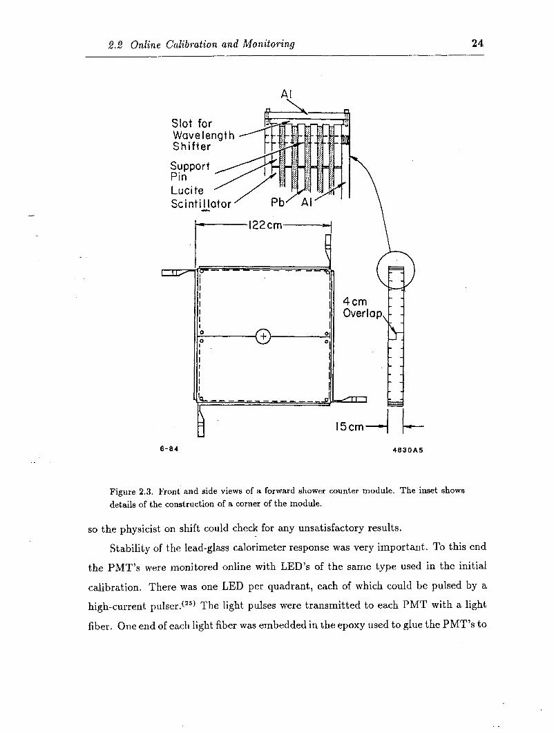
z = f4.0 m. The forward shower counters (FSC) (see fig. 2.3) were constructed
from alternating sheets of lead (0.6 cm) and scintillator (1.3 cm) in modules which
were 6 radiation lengths (X0) thick. The scintillator layers in each module were
ganged together and read out by four wavelength shifter bars, each viewed by a single
PMT. Two such modules were used for each of the inner FSC’s, which overlapped the
angular region covered by the central detector and extended the coverage to within
100 mr of the beamline. Two crossed planes of PWC’s, constructed of the same type
of aluminum extrusion used firr the CPWC’s, were inserted between the modules to
measure the spatial position of electromagnetic showers. The outer FSC’s, which
covered the region between 21 mr and 120 mr from the beamline, consisted of three
6X0 modules each. PWC’s were again located at a depth of 6X0, between the first
and second modules. The additional material in the outer calorimeters reduced the
probability that a photon would fail to convert in the detector, and provided good
containment of showers from e+e- at low angles. The forward calorimeters provided a
veto and calibration system for the ASP experiment as well as a luminosity monitor
for the PEP storage ring.
Between the inner and outer FSC’s on each side were drift chambers, located
at 2 = f1.9 m and z = f 3.0 m. At each location there were two drift-chamber
planes to measure both the x and y coordinates, so as to provide precise charged
particle tracking between 21 and 100 mr. The drift chambers were operated with a
gas mixture of 48.2% argon, 48.2% ethane and 1.6% ethyl alcohol.
2.2 Online Calibration and Monitoring
The entire detector was continuously monitored, with readings every four min-
utes; any voltage or current which strayed outside the prescribed boundaries would
cause the data acquisition system to immediately shut down and would sound an
alarm. A calibration was performed once during each eight-hour shift to provide up-
to-date constants and to detect any serious hardware malfunctions. In addition, a
small fraction of the data was analyzed as it was being recorded to check for more
subtle problems. At the end of each run the results of the analysis were printed out
2.2 Online Calibration and Monitoring 24
ScintiJator ’ Pb/Al’ ” \
6-64 4830A5
Figure 2.3. Front and side views of a forward shower counter module. The inset shows details of the construction of a corner of the module.
so the physicist on shift could check for any unsatisfactory results.
Stability of the lead-glass calorimeter response was very important. To this end
the PMT’s were monitored online with LED’s of the same type used in the initial
calibration. There was one LED per quadrant, each of which could be pulsed by a
high-current pulser. (25) The light pulses were transmitted to each PMT with a light
fiber. One end of each light fiber was embedded in the epoxy used to glue the PMT’s to
25 Experimental Apparatus
the lead-glass bars. The output of each LED was monitored by a reference PMT which
also viewed a small NaI(T1) scintillator crystal doped with 24*Am(2S) which served
as a stable light source. (27) This system was used to provide a relative calibration of
the PMT’s, but it was not used for an absolute calibration as the transmission of the
light fiber connections drifted with time, and also the LED spectrum did not cover
the full range of the PMT photocathode spectral sensitivity. The reliability of the
phototubes was high: fewer than 1% of the tubes failed for any reason over the entire
course of the experiment. - -
2.3 The Trigger
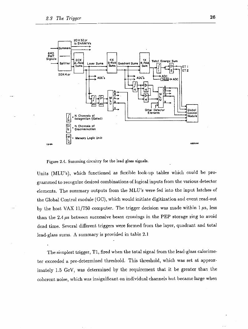
The signals from each of the 632 PMT ‘s used to read out the lead-glass bars were
first sent through a passive transformer splitter. One of the two resulting signals was
sent to a SHAM-BADC system, (28) a sample-and-hold module followed by an analog-
to-digital converter which also performed pedestal subtraction and gain correction.
This provided the primary read-out of the calorimeter. The other half of the signals
were summed, first in groups of eight from adjacent bars in the same layer, then with
the other groups of eight in each layer to form 20 analog signals, one from each of the
five layers in the four lead-glass quadrants.
.
The layer sums were then fanned out; see fig. 2.4. One copy was digitized and
read out to provide a redundancy check against the SHAM-BADC system. It ‘was also
used in the offline code to correct for saturation in the BADC, which occurred when
more than about 1.2 GeV was deposited in a single bar. Another copy was summed
to provide the total quadrant signals, which were summed in turn to form an analog
signal proportional to the total calorimeter energy. These sums were also digitized
and read out. A third copy of the layer-sums was integrated and discriminated, as
were the quadrant and total lead-glass sums, to provide digital inputs for the trigger
logic. c2’)
The ASP trigger decision was based on the discriminated signals from the layer,
quadrant and total lead-glass sums, together with discriminated signals from the
FSC’s and veto scintillators. These digital inputs were sent to two Memory Logic
2.3 The Trigger 26
Signals -+ 20x 4x 4 Splitter Layer Sums
-b 4s;F”mLd
, 5zF$ Quadrant sums
-
20X4pr - 1
‘. ADCi ‘- ADC I Ant-
--L-P+ 11 I I-
Other Detector Elamenls
N Channels of lntegratlon (Goled)
- u y = Memory Logic Unit U
19-m .ISDAl
Figure 2.4. Summing circuitry for the lead glass signals.
Units (MLU’s), which functioned as flexible look-up tables which could be pro-
grammed to recognize desired combinations of logical inputs from the various detector
elements. The summary outputs from the MLU’s were fed into the input latches of
the Global Control module (GC), h h w ic would initiate digitization and event read-out
by the host VAX 11/750 computer. The trigger decision was made within 1 ps, less
than the 2.4~s between successive beam crossings in the PEP storage ring to avoid
dead time. Several different triggers were formed from the layer, quadrant and total
lead-glass sums, A summary is provided in table 2.1
The simplest trigger, Tl, fired when the total signal from the lead-glass calorime-
ter exceeded a pre-determined threshold. This threshold, which was set at approx-
imately 1.5 GeV, was determined by the requirement that it be greater than the
coherent noise, which was insignificant on individual channels but became large when
27 Experimental Apparatus
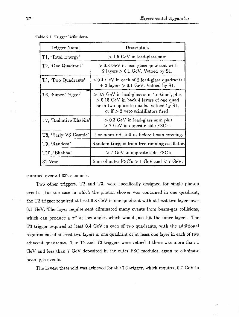
Table 2.1. Trigger Definitions.
Trigger Name Description
Tl, ‘Total Energy’ > 1.5 GeV in lead-glass sum
T2, ‘One Quadrant’ > 0.8 GeV in lead-glass quadrant with 2 layers > 0.1 GeV. Vetoed by Sl.
T3, ‘Two Quadrants’ > 0.4 GeV in each of 2 lead-glass quadrants + 2 layers > 0.1 GeV. Vetoed by Sl.
L T6, ‘Super-Trigger’ > 0.7 GeV in lead-glass sum ‘in-time’, plus
> 0.15 GeV in back 4 layers of one quad or in two opposite quads. Vetoed by Sl,
or if- > 2 veto scintillators fired.
T7, ‘Radiative Bhabha’ > 0.3 GeV in lead-glass sum plus > 7 GeV in opposite side FSC’s.
T8, ‘Early VS Cosmic’ 1 or more VS, > 5 ns before beam crossing.
T9, ‘Random’ Random triggers from free-running oscillator
TlO, ‘Bhabha’ > 7 GeV in opposite side FSC’s
Sl Veto Sum of outer FSC’s > 1 GeV and < 7 GeV.
summed over all 632 channels.
.
Two other triggers, T2 and T3, were specifically designed for single photon
events. For the case in which the photon shower was contained in one quadrant,
the T2 trigger required at least 0.8 GeV in one quadrant with at least two layers over
0.1 GeV. The layer requirement eliminated many events from beam-gas collisions,
which can produce a r” at low angles which would just hit the inner layers. The
T3 trigger required at least 0.4 GeV in each of two quadrants, with the additional
requirement of at least two layers in one quadrant or at least one layer in each of two
adjacent quadrants. The T2 and T3 triggers were vetoed if there was more than 1
GeV and less than 7 GeV deposited in the outer FSC modules, again to eliminate
beam-gas events.
The lowest threshold was achieved for the T6 trigger, which required 0.7 GeV in
i- i.

2.3 The Trigger 28
the total lead-glass sum. In addition, at least 0.15 GeV was required in the back four
layers of one and only one quadrant, or in two opposite quadrants. No more than two
of the four veto scintillators surrounding the central tracker were allowed to be above
threshold, and the lead-glass energy was required to be ‘in-time’, within 4120 ns of the
beam crossing. Finally, the T6 trigger was vetoed by the same FSC veto applied to
the T2 and T3 triggers. The combined efficiency of the ‘lead-glass triggers’, Tl,T2,T3
and T6, is shown in fig. 2.5 as a function of total-lead glass energy, measured using
- kinematically-fit radiatiBBhabhas.
E I 001 * 0 1 2 3 4 5
Enerqy, GeV Figure 2.5. Efficiency of lead-glass triggers a.s a function of total lead-glass
The T7 trigger was designed to log out radiative Bhabha events with two forward
tracks and one track in the glass. This trigger required at least 0.3 GeV in the lead
glass plus a coincidence between two FSC’s with at least 7 GeV on either side of
the detector. Because the T7 triggei’ threshold was significantly lower than the other
lead-glass trigger thresholds, it was useful for studying the performance of the other
triggers. In addition, kinematically-fitted radiative Bhabhas provided a means of
understanding many aspects of the detector performance.
Other diagnostic triggers included the early VS cosmic trigger, which fired when a
charged particle was detected in the veto scintillators surrounding the central tracker
energy.

29 Experimental Apparatus
in a 15 ns time window which ended 5 ns beFore the beam crossing. Low-angle
Bhabhas in which more than 7 GeV was deposited in both inner or both outer FSC
modules were recorded for luminosity studies. (Because of the high event rate for
this process a pre-scale factor of 600 for the outer and 20 for the inner FSC’s was
imposed.) Random beam crossings were also recorded to study detector occupancy.
The total trigger rate of the ASP detector was typically 4.5 Hz, and the live time was
typically about 90%.
3
Event Reconstruction
-
The raw data consists of signals from each detector element. These signals must
be calibrated to correct for channel-to-channel variations and to determine the abso-
lute scale. Then pattern recognition, or ‘tracking’, must be performed on all of the
signals to determine the particle trajectories in an event. Once the events have been
tracked, the event selection can be made. In this chapter the calibration and tracking
procedures for the lead-glass calorimeter are described.
3.1 Off-line Calibration
Cosmic ray muons recorded by the early VS cosmic trigger were used to perform
an off-line calibration of the PMT response. This sample was tracked and the signal
deposited in each bar was corrected for path length. The average path-corrected
signal displayed a strong dependence on both the distance of the track from the PMT
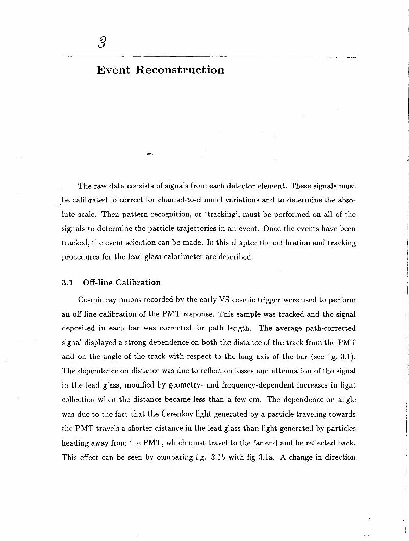
and on the angle of the track with respect to the long axis of the bar (see fig. 3.1).
The dependence on distance was due to reflection losses and attenuation of the signal
in the lead glass, modified by geometry- and frequency-dependent increases in light
collection when the distance became less than a few cm. The dependence on angle
was due to the fact that the Cerenkov light generated by a particle traveling towards
the PMT travels a shorter distance in the lead glass than light generated by particles
heading away from the PMT, which must travel to the far end and be reflected back.
This effect can be seen by comparing fig. 3.lb with fig 3.la. A change in direction
I j- i’
j.
j

31 Event Reconstruction
also changes the angle of incidence of the light as it travels down the bar by internal
reflection and hence changes the total distance travelled in the glass.
Figure 3.1. Attenuation in the lead glass bar as a function of distance and angle. In a), the track is pointing towards the PMT at an angle of 45’, and in b) it is pointing away.
.
Each lead-glass quadrant was oriented in a different direction, with some PMT’s
pointing up, some down and others oriented horizontally. Therefore the angular
distribution of the predominantly down-going cosmic rays with respect to the axis of
the lead-glass bars was different in each quadrant. This resulted in a different average
path-length corrected signal in each quadrant. To compensate for attenuation effects,
a correction was applied on an event-by-event basis. The correction factor was a
function of both the distance of the track from the PMT and the angle of the track
with respect to the bar, taken from a look-up table compiled from plots such as
those in fig. 3.1. The peak was extracted from the resulting spectrum for each PMT
and this value was used to normalize its response. Most PMT’s had multiplicative
normalization factors in the range from .5 to 1.5, with a handful extending up to 2.
This cosmic-ray calibration was more accurate than the one which had been

--
3.2 Energy Determination 32
performed with an LED prior to installation because the spectral response of the
PMT’s was integrated over the correct frequency range of cerenkov light. In addition,
any channel-to-channel variation in the electronics used to read out the PMT’s was
automatically included in the calibration. This calibration was also used to check for
evidence of radiation damage, which would cause a time dependent decrease in the
transmission of the lead-glass bars. No significant decrease in response was observed.
Moving the detector away from the beampipe during injection and the installation of
lead-brick walls were responsible for a significant reduction in the integrated radiation
dose seen by the lead glass, and the addition of cerium to the lead glass prevented
any significant damage from the radiation which was absorbed.
-3.2 Energy Determination -
The Cerenkov light collected from an electromagnetic shower in lead glass is pro-
portional to the integrated path length traveled by all charged particles in the shower ”
which are above the Cerenkov threshold (0.7 MeV for electrons), and is therefore pro-
portional to the energy of the shower. The light is transmitted by internal reflection
down the bar to the PMT. After correcting for the effects of differing PMT gains
using the constants derived in the off-line calibration, the signals must be corrected
for attenuation. The event was tracked first, and then the same look-up table used in
the off-line calibration was applied, using the track parameters to calculate the angle
and distance of the shower from the PMT.
Further corrections were made for leakage, pre-radiation and the absorption of
energy in the non-active material inside the calorimeter. The amount of energy which
leaks out of the calorimeter is a function of the total thickness (in radiation lengths)
and the incident particle energy. Using the EGS Monte Carlo c30) to simulate elec-
tromagnetic cascades, the following empirical approximation was derived to correct
for leakage on the mean:
&leak = 2.0 X esa3-” X Eincla4 GeV (1)
where Eleak is the energy lost in GeV, X is the thickness of the detector in radiation

33 Event Reconstruction
lengths along the trajectory of the track, and Einc is the incident energy in GeV. The
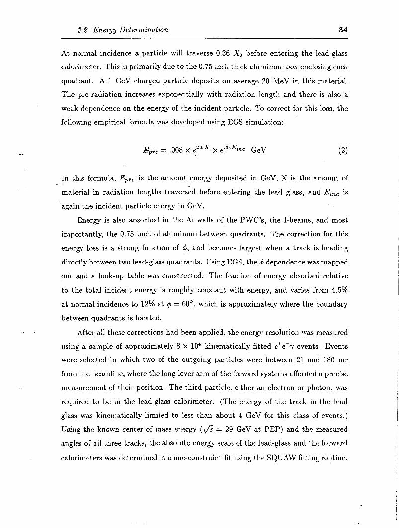
thickness of the detector at 4 = 90’ varied from 10 X0 at 0 = 90’ to 20 X0 at 0 = 30’.
The thinnest part of the detector was in the corners between quadrants, where X cz 8
X0 at 8 = 90’; see fig. 3.2. For photons, the estimated point of conversion in the lead
glass was also used in the calculation of X. A first estimate of Eleak was obtained by
substituting the observed energy for Einc, then Eobs + Bleak was substituted for Einc and this procedure was iterated until the estimate of Eleak converged to within 5% of
- the previous estimate for Elea%. For a 1 GeV particle at normal incidence, the mean
energy lost is about 100 MeV, or lo%, and at 8 = 30” this is reduced to 0.5%. The
corresponding numbers for a particle of 14.5 GeV are 30% and 1.5%. This correction
is clearly most important at wide angles. No attempt was made to take into account
fluctuations in leakage.
12.5
2.5
0.0
Phi, Deqrees
Figure 3.2. Thickness of the lead-glass calorimeter in radiation lengths vs. 4, at 0 = 90”.
Radiation of charged particles in the material preceding the calorimeter and
absorption of energy in the non-active material have also been studied using EGS.
I
i.:
9.2 Energy Determination 34
At normal incidence a particle will traverse 0.36 X0 before entering the lead-glass
calorimeter. This is primarily due to the 0.75 inch thick aluminum box enclosing each
quadrant. A 1 GeV charged particle deposits on average 20 MeV in this material.
The pre-radiation increases exponentially with radiation length and there is also a
weak dependence on the energy of the incident particle. To correct for this loss, the
following empirical formula was developed using EGS simulation:
- &me = .008 x ezesx x eao4@nc GeV
In this formula, Eyre is the amount energy deposited in GeV, X is the amount of
material in radiation lengths traversed before entering the lead glass, and Einc is
. again the incident particle energy in GeV.
Energy is also absorbed in the Al walls of the PWC’s, the I-beams, and most
importantly, the 0.75 inch of aluminum between quadrants. The correction for this
energy loss is a strong function of 4, and becomes largest when a track is heading
directly between two lead-glass quadrants. Using EGS, the 4 dependence was mapped
out and a look-up table was constructed. The fraction of energy absorbed relative
to the total incident energy is roughly constant with energy, and varies from 4.5%
at normal incidence to 12% at 4 = 60°, which is approximately where the boundary
between quadrants is located.
After all these corrections had been applied, the energy resolution was measured
using a sample of approximately 8 x lo4 kinematically fitted e’e-7 events. Events
were selected in which two of the outgoing particles were between 21 and 180 mr
from the beamline, where the long lever arm of the forward systems afforded a precise
measurement of their position. The- third particle, either an electron or photon, was
required to be in the lead-glass calorimeter. (The energy of the track in the lead
glass was kinematically limited to less than about 4 GeV for this class of events.)
Using the known center of mass energy (& = 29 GeV at PEP) and the measured
angles of all three tracks, the absolute energy scale of the lead-glass and the forward
calorimeters was determined in a one-constraint fit using the SQUAW fitting routine.
,

35 Event Reconstruction
c31) Once the overall normalization had been established, the calorimeter resolution
was determined by plotting the difference between the measured energy and the fitted
energy. The results for the lead glass are displayed as a function of energy in fig. 3.3.
The curve is well described by the resolution function
Enerqy, GeV
Figure 3.3. Resolution in the lead glass bar as a function of energy.
3.3 Tracking
The tracking proceeded in several stages. The boundaries of each shower were
first determined with a cluster-finding algorithm. Fluctuations in the development
of an electromagnetic shower create gaps in the pattern of energy deposition, while
on the other hand two showers which are close together in the plane of a quadrant
may overlap. The clustering algorithm therefore allowed gaps, but was also sensitive
3.3 Tracking 36
to peaks and valleys and would start a new cluster when large enough fluctuations
in signal were encountered. Clusters were not continued across quadrant boundaries;
clusters from a single shower which extended into adjacent quadrants were combined
at a later stage of the tracking.
--
A two-dimensional total least squares fit was then performed for each cluster.
This fit found the axis about which the sum of the squares of the perpendicular
distances to each bar, Di, was minimized. The signal in each bar corrected for PMT
gain, Si, was used to w&ght each term. (The attenuation correction could not be
applied at this stage because the angles of the track were not yet determined.) The
quantity to be minimized was:
MW2 = c SiD,2 . (3) i
A slope and intercept in the plane of the quadrant (xz or yz) were extracted from
this fit.
.
The signals observed in the central PWC’s, the central tracker, and the forward
systems were all tracked independently and combined with the lead-glass clusters to
reconstruct an event topology. To accomplish this, the track segments from each
system were reduced to vector and error matrices. A topology finding routine then
identified the segments from each system which could belong together in a track. A
least-squares fit was performed, and if the x2 was satisfactory a track was created
utilizing all the information from the various systems. If the x2 was unsatisfactory,
the segment which contributed the most to the x2 was dropped and the fit was tried
again. Clusters from a shower which crossed the boundary between two quadrants
were combined in a similar fashion: The clusters were required to match based on
a x2 formed from their 0 values and errors, and information from the other central
tracking systems was used in the fit. Tracks from minimum-ionizing particles were
treated in the same way as electromagnetic showers; the tracking code worked equally
well for both.
Ambiguities arose in matching lead-glass clusters and PWC clusters when there
37 Event Reconstruction
were multiple tracks per quadrant. For charged tracks ihis could usually be resolved
by the central tracker. However if there were multiple neutral tracks in a quadrant,
the tracking algorithm had to rely on a comparison of the signal deposited in each
layer of the lead glass and PWC clusters. From this comparison the best match
between the lead-glass and central PWC systems was determined, based on how well
the patterns of energy deposition in the two systems matched. When two showers
had very different patterns this method worked well; however if they were similar the
- likelihood of choosing the wrahg combination increased. Because of this limitation
* the tracking worked best for low multiplicity events.
Bhabha events were used to study the angular resolution of the lead glass. The
quantity which is actually measured with the lead-glass calorimeter is Op, the polar
angle projected into the xz or yz plane. The resolution in 6p improves at lower angles
because the lever arm is greater as the distance to the interaction point increases. The
resolution averaged over all angles is d = 1.9’. The angular resolution of the lead glass
was also a function of energy, becoming worse at lower energies because the position
of the shower centroid was less well measured. For showers from kinematically fitted
radiative Bhabha events, ranging in energy from 0.5 to 3 GeV, the average resolution
was 0 = 4.4’.
.
The spatial origin of a shower in the lead glass was characterized by the distance
of closest approach to the beamspot in the xz or yz plane, R,. This quantity was used
because the resolution is then approximately independent of &. For 14.5 GeV showers
from Bhabha events the R, distribution was Gaussian, with an average resolution of
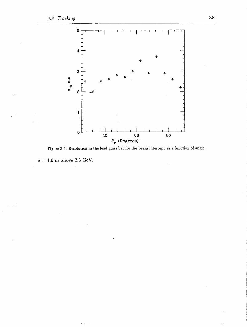
u = 2.6 cm. The resolution is shown as a function of BP in fig. 3.4. For low-energy
showers, such as those from radiative Bhabha events, the distribution was Gaussian
with 0 = 2.8 cm and a small exponential tail.
Timing information from the lead glass was obtained for each quadrant, and
corrections were applied using the tracking information. Both the path length of
the track from the interaction point to the lead-glass calorimeter and the distance
the light traveled down the bar to the PMT were taken into account. After these
corrections were applied the timing resolution was 0 = 1.2 ns for a 1 GeV shower and
--
L
4-
3-
!!I :4
ba’ 2- dd
l-
4
4 4 4 4
4 4
4 4
4
4-
I 4
01‘ ” ” ” ” ” ” ” I’ 40 60 80
8, (Degrees)
Figure 3.4. Resolution in the lead glass bar for the beam intercept as a function of angle.
u = 1.0 ns above 2.5 GeV.

4 Event Simulation
-
-About 5% of all Q’S and 15% of all Q”S produced in two-photon interactions
which subsequently decayed into two photons were included in the final data sample.
Some did not decay into the sensitive parts of the detector, and others failed to fire the
trigger. Some events were removed by cuts designed to reduce backgrounds from other
processes. Understanding the detector acceptance and event selection efficiency is a
very important aspect of the analysis. To achieve this with a high degree of accuracy,
Monte Carlo methods and a detailed model of detector response *are employed to
perform the calculations.
The first step is to generate 77 and q’ events according to the two-photon pro-
duction cross section. This procedure is described in section 4.1. Next the generated
photons are passed through the detector simulation routines, described in section 4.2.
A comparison of the simulation with real data is also presented in this section, to
show how well the detector response is reproduced. The trigger logic is then applied
to the raw data, as described in section 4.3, to determine whether the generated event
would have fired the trigger and been logged out.
The simulated events can be tracked and processed using the same event selection
routines which are used to filter the data. This is the subject of the next chapter.

4.1 Event Generation 40
4.1 Event Generation
-
The differential cross section for two-photon production of 7 or 7’ mesons, eq.
1.14, has been formulated by Vermaseren(32) in a form which is convenient for nu-
merical integration. A Monte Carlo based on this formulation has been used which
generates unweighted events and simultaneously calculates the total cross section,
assuming that Pyy= 1 keV. The cross sections are therefore calculated in nb/keV, so
that Prr is given by the ratio of the experimentally obtained value for the cross section
to the calculated cross stiion. The processes e+e’ + (e+e’)q and e+e- + (e+e-)q’
were generated with M,, = 548.8 MeV and iWvl = 957.6 MeV; all of the generated
_ events were made to decay into two photons, the final state of interest for this analysis.
The Q” dependence of the cross section for two-photon production of the q and
71’ mesons is illustrated in table 4.1 , where the calculated cross sections are given
with no form factor and also with the form factor of Brodsky and Lepage,(33)
qq:>!a = 1
(1+ &(l+ &)’ M2 - .68GeV2. (4.1)
This form factor differs from the p form factor only in the value of the mass, which
for the p form factor is M2 = MS = .59GeV2. The total production cross section is
significantly suppressed by the form factor, but for events within the ASP detector
acceptance (defined as 20° < 8, < 160’ for both photons, and both electrons within
21 mr of the beamline) the difference in the cross section with and without the form
factor is slight, a 1.5% reduction for q events and 1.8% for 7’ events. This is because
the requirement that the scattering angle of the electrons be less than 21 mr limits
the maximum Q” to less than .093GeV2.
Events were generated about the measured beam positions with a gaussian dis-
tribution characterized by (T = 0.5 cm in 2 and $ and cr = 1.5 cm in i. The position
of the beamspot was measured using the forward drift chambers; it varied with time
in i and $ but remained the same in 2. Run numbers from both data cycles were
chosen in the event generation process, using luminosity weighting. This ensured that
run-dependent constants, such as the beam spot position, the PMT gain factors and
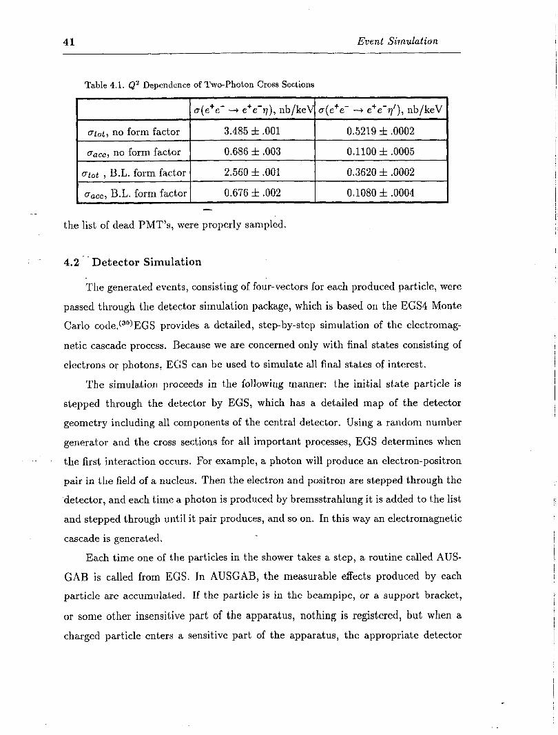
41 Event Simulation
Table 4.1. Q2 Dependence of Two-Photon Cross Sections
1 o(e+e- + e+e’v), nb/keVf a(e+e- -+ e+e-q’), nb/keV
alot, no form factor 3.485 f .OOl 0.5219 f .0002
dacc, no form factor 0.686 f .003 0.1100 f .0005
atot , B.L. form factor 2.560 f .OOl 0.3620 f .0002
cr.,,, B.L. form factor I 0.676 f .002 I 0.1080 f .0004
the list of dead PMT’s, were properly sampled.
4.2 - Detector Simulation
Tl g le enerated events, consisting of four-vectors for each produced particle, were
passed through the detector simulation package, which is based on the EGS4 Monte
Carlo code.c3’)EGS provides a detailed, step-by-step simulation of the electromag-
netic cascade process. Because we are concerned only with final states consisting of
electrons or photons, EGS can be used to simulate all final states of interest.
The simulation proceeds in the following manner: the initial state particle is
stepped through the detector by EGS, which has a detailed map of the detector
geometry including all components of the central detector. Using a random number
generator and the cross sections for all important processes, EGS determines when
the first interaction occurs. For example, a photon will produce an electron-positron
pair in the field of a nucleus. Then the electron and positron are stepped through the
detector, and each time a photon is produced by bremsstrahlung it is added to the list
and stepped through until it pair produces, and so on. In this way an electromagnetic
cascade is generated.
Each time one of the particles in the shower takes a step, a routine called AUS-
GAB is called from EGS. In AUSGAB, the measurable effects produced by each
particle are accumulated. If the particle is in the beampipe, or a support bracket,
or some other insensitive part of the apparatus, nothing is registered, but when a
charged particle enters a sensitive part of the apparatus, the appropriate detector
4.2 Detector Simulation 42
response is simulated.
The simulation of electromagnetic showers using EGS is very CPU intensive, and
the computer time required grows linearly with energy. To reduce the time required
somewhat, there is an energy cutoff in EGS below which a particle is not transported
any further. This cutoff is adjustable, and has been set to 1.5 MeV for electrons
and 0.5 MeV for photons. The detector response to the remaining energy deposit is
estimated and accumulated in AUSGAB when the particle is discarded.
The passage of a charged particle through lead glass results in the emission of --
Cerenkov light. The amount of Cerenkov light deposited by each charged particle
in the lead glass is proportional to the step length x(1 - $), where p = z is the
particle velocity divided by the speed of light and ,& = k is the threshold for emission
of Cerenkov light in a medium of refractive index n. (In the lead glass used in this
experiment, n = 1.58 and PC = .63.) The light is emitted in a cone around the
trajectory of the particle with an opening angle given by 0, = arccos(-&). For a
particle traveling close to the speed of light in lead glass Bc N 50°. The Cerenkov
light travels down the lead-glass bar by internal reflection, eventually reaching the
photo-cathode of the PMT which is glued to one end.
In order to simulate this process exactly, one would need a very sophisticated
algorithm to trace the light rays from the Cerenkov cone as they reflect down the
length of the lead-glass bar, determining the loss by attenuation. Instead, we have
used a look-up table which gives the attenuation factor as a function of the distance
of the particle from the PMT and the angle of the primary particle which initiated the
shower, This look-up table was compiled using high-energy muons from cosmic-ray
data. It is the inverse of the look-up table used to correct the raw data for attenuation
after the tracking has been performed, as described in the previous chapter. After
accumulating all the Cerenkov signals in an event, the gain factor for each PMT is
applied to the data. This factor is set to zero for any dead PMT’s.
Attenuation and PMT gain must be included in the simulated data for two rea-
sons. First, the trigger decision is based on raw data, so these effects are important
in correctly estimating trigger efficiency. Secondly, it is important to make the simu-
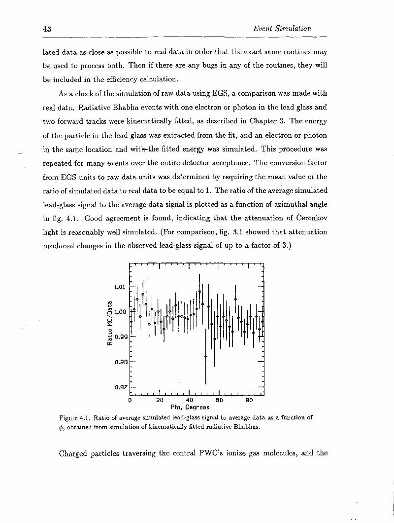
43 Event Simulation
lated data as close as possible to real data in order that the exact same routines may
be used to process both. Then if there are any bugs in any of the routines, they will
be included in the efficiency calculation.
--
As a check of the simulation of raw data using EGS, a comparison was made with
real data. Radiative Bhabha events with one electron or photon in the lead glass and
two forward tracks were kinematically fitted, as described in Chapter 3. The energy
of the particle in the lead glass was extracted from the fit, and an electron or photon
in the same location and witkthe fitted energy was simulated. This procedure was
repeated for many events over the entire detector acceptance. The conversion factor
from EGS units to raw data units was determined by requiring the mean value of the
ratio of simulated data to real data to be equal to 1. The ratio of the average simulated
leadiglass signal to the average data signal is plotted as a function of azimuthal angle
in fig. 4.1. Good g a rcement is found, indicating that the attenuation of Cerenkov
light is reasonably well simulated. (For comparison, fig. 3.1 showed that attenuation
produced changes in the observed lead-glass signal of up to a factor of 3.)
t
rl I I I 0 20 40 60 80
Phi, Deqrees Figure 4.1. Ratio of average simulated lead-glass signal to average data as a function of 4, obtained from simulation of kinematically fitted radiative Bhabhas.
Charged particles traversing the central PWC’s ionize gas molecules, and the

4.2 Detector Simulation 44
liberated electrons drift along the electric field lines to the sense wire. Near the sense
wire the electrons begin to ionize other gas molecules and an avalanche is created,
which provides signal amplification. If there are many charged particles, a saturation
point is reached and the response becomes non-linear. In order to simulate this
process, a signal proportional to the energy lost by each charged particle in the gas
volume of the central PWC’s is accumulated in AUSGAB. When the simulation of
the event is complete, the signal in each PWC cell is corrected to include non-linear
- saturation effects. A comparison of the simulated central PWC signal with data has
been performed using kinematically fitted radiative Bhabha events, and the ratio as a
function of track energy is shown in fig. 4.2. Reasonably good agreement is obtained
for tracks above 250 MeV; below this-energy the fits are not very reliable. The ratio
of Monte Carlo to data drops below 1 as the track energy increases; however for-this
analysis most tracks are in the range .275 - 1. GeV and are not much affected by the
disagreement.
1.25 -
0.25 -
o.oo- ’ I ’ ’ ’ ’ I ’ ’ ’ ’ I ’ ’ ’ ’ I ’ ’ ’ ’ 0.5 1 1.5 2 2.5
Track Enerqy, GeV Figure 4.2. Ratio of average simulated central PWC signal to average data as a function of track energy, obtained from simulation of kinematically fitted radiative Bhabhas.
The energy deposited by charged particles in the central tracker is accumulated
after applying a Q-dependent correction taken from an analysis of real data. Charge

45 Event Simulation
division of the signal is obtained by dividing the signal into two parts proportional to
the distance from each end. This results in a simulation which is more perfect than in
reality, as it does not include the sometimes large systematic errors caused by offsets
due to noise or cross-talk which affect the real data.
The veto scintillators surrounding the central tracker are simulated by accumu-
lating the energy deposited by each charged particle, multiplied by an exponential
attenuation factor. The signal is divided into two according to the distance of the
track from the PMT’s mounted on each end.
For the forward shower counters and forward PWC’s, the electromagnetic shower
is not fully simulated. Instead, look-up tables are used to simulate the response as
a function of energy and position, reproducing the irregular pattern of radiation
damage to the scintillator in the forward shower counters. This method saves CPU
time, especially when the forward-going particle is a scattered electron with close to
beam energy. The forward drift chambers are not simulated, and neither are the
time-of-flight counters.
Detector noise is included in the simulation by overlaying the-simulated events
with real events logged out by the random trigger. Because most beam crossings do
not result in any interaction, these random triggers represent the quiescent detector
response with beam present in the storage ring. The random events have been lumi-
nosity weighted, with more events taken from periods with high beam currents and
high luminosity.
4.3 Trigger Simulation
The ASP trigger has already been described in Chapter 2. The most important
trigger for this analysis was the T6 trigger, also called the ‘super trigger’ because it
has the lowest energy threshold in the lead-glass, about 0.7 GeV. The mass of the
7 is 549 MeV, which is below this threshold. This results in a significant trigger
inefficiency for 77 ---) 77 events (about 50%), and means that the trigger must be very
well understood. To achieve this, a detailed simulation involving threshold effects for
every input to the trigger logic has been performed.

4.3 Trigger Simulation 46
The inputs to the trigger logic are discriminated signals from the lead glass, the
forward shower counters, and the veto scintillators. From the lead glass alone there
are 36 logical signals, obtained by discriminating the total lead-glass energy at four
different levels, the quadrant sums at two different levels, the twenty layer sums and
the sum of the back four layers in each quadrant. Each discriminator threshold may
vary slightly from others set at the same level, and the rise may also vary. Over time
the response remained very constant due to the uniform temperature maintained in
- the electronics building. -
To duplicate this threshold behavior, T7 triggers were selected. This trigger
requires a very low threshold in the lead glass, about 0.3 GeV, in coincidence with
significant energy in the forward shower counters on either side. The events thus
selected are primarily radiative Bhabha events. This data set provides an unbiased
sa.mple with which to study the other lead-glass triggers, because the T7 threshold is
so much lower than any of the others.
Using the T7 triggers, the threshold response for each trigger input was obtained
as a function of raw PMT signal. These histograms were then stored as look-up
tables. To determine whether a simulated event had fired the trigger, the simulated
raw counts were summed and ‘discriminated’ using a random number generator and
interpolating the look-up tables for each input. Once all trigger inputs had been
simulated the trigger logic was applied, and the trigger arrays were filled just as they
are for real data.
For the forward shower counters a different approach was necessary because
the simulation of raw energy was not very accurate for these devices, due to an
uneven pattern of radiation damage to the scintillator. Instead, the probability for
the forward triggers to fire was calculated as a function of the energy and position of
the incident particle. To do this, radiative Bhabha events with at least one forward
track were selected in which the total lead-glass energy trigger had fired. This sample
was therefore independent of the forward trigger. A kinematic fit was used for the
trajectories of the forward tracks.
Simulation of the veto scintillator trigger bits was unnecessary because only the
47 Event Simulation
early VS cosmic trigger required them. Although the T6 trigger was vetoed if 3
or more veto scintillators were above threshold, this had a negligible effect on the
trigger efficiency for events with 2 or fewer charged tracks. This was determined
using a sample of events recorded with a special pre-scaled T6 trigger which did not
have this veto.
5
Event Selection
L- -
Approximately 30 million events recorded by the ASP detector were logged to
.tape. From this initial sample a few thousand events were selected for the final data
sample. This reduction of four orders of magnitude was achieved in several stages.
The final state selected by this analysis has two photons in the lead glass calorime-
ter from the decay of an v or 7’. The two photons are typically back to back in the
azimuthal plane and acollinear in the plane containing the beamline. The electrons
escape down the beampipe and are not observed. The total energy is much less than
the total center-of-mass energy of 29 GeV. The specific criteria designed to select
events with these distinctive characteristics are described in this chapter.
5.1 Production First Pass
All of the raw data was first processed by a filter designed to reject obvious junk,
such as cosmic rays and beam-gas interactions, as quickly and efficiently as possible.
Cosmic ra,y events were rejected by exploiting the fact that they are distributed
uniformly in position and time instead of originating at the interaction point in time
with the beam crossing. If the event time was well measured, it was required to occur
within 5cr of the beam crossing. Events were rejected in which the lead-glass track
closest to the origin passes more than 20 cm away, or in which the central PWC track
closest to the origin is more than 20 cm from the origin in the xy plane. (The energy
deposition pattern was required to be uniform, as expected from a minimum-ionizing

49 Event Selection
particle, for tracks which failed these cuts.) Beam-gas events and ‘beam-burps’ were
eliminated by rejecting events with more than 80 tubes hit in the central tracker.
After rejecting identified cosmic rays and beam-gas events, a positive signature
from each event was required in the form of at least oue lead-glass cluster with more
than 60 MeV of energy, originating from the interaction point. To originate from the
interaction point the track was required to have a distance of closest approach to the
origin, R = )zI sin 0, of less than 30 cm. This was a very loose cut and was designed
- to accept any event which was-even remotely interesting.
About 12 million events satisfied these criteria. They were then tracked and
written out for further analysis. Diagnostic events, such as random triggers and VS
cosmic triggers, were skimmed off separately for detector studies.
5.2 Analysis First Pass
In the first pass of this analysis, a very loose selection is made which includes
charged events. In particular, events from the process e+e- 3 (e+e-)e+e-, which
resemble the 7 --t yr topology, are retained for efficiency studies. Ten percent of the
events on the production first pass tapes survive these cuts, described below.
The first requirement is that the event should be in the detector acceptance and
have the correct multiplicity. At least two and not more than three lead-glass clusters
with energy greater than 100 MeV and with 8, > 20° are required. Lead-glass clusters
which are split between two quadrants, or small clusters which are fluctuations from
a large cluster, are combined before determining the total. Projected theta is defined
as tan e, _ sine X mad cos 4, I sin 4) -
cos e
Projected theta can be thought of as the polar angle, 8, projected into the xz or yz
plane. Using 8, to define the detector acceptance gives a square cutoff at the ends,
corresponding to the box-like shape of the ASP detector.
The event is then required to have a lead-glass trigger, either Tl,T2,T3 or T6,
using the trigger definitions given in chapter 2. This requirement is actually imposed
when the data are collected, but it is re-iterated to define the trigger criteria explicitly
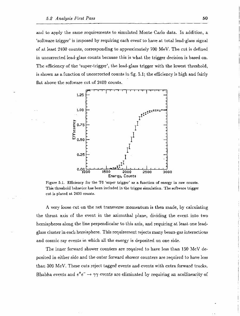
5.2 Analysis First Pass 50
and to apply the same requirements to simulated Monte Carlo data. In addition, a
‘software trigger’ is imposed by requiring each event’ to have at total lead-glass signal
of at least 2400 counts, corresponding to approximately 700 MeV. The cut is defined
in uncorrected lead-glass counts because this is what the trigger decision is based on.
The efficiency of the ‘super-trigger’, the lead-glass trigger with the lowest threshold,
is shown as a function of uncorrected counts in fig. 5.1; the efficiency is high and fairly
flat above the software cut of 2400 counts.
0.25 I TI I
II &&,I ‘ 1 ,
J ’ 1 “Yboo 1500 2000 2500 3000
Enerqy, Counts
Figure 5.1. Efficiency for the T6 ‘super trigger’ as a function of energy in raw counts. This threshold behavior has been included in the trigger simulation. The software trigger cut is placed at 2400 counts.
A very loose cut on the net transverse momentum is then made, by calculating
the thrust axis of the event in the azimuthal plane, dividing the event into two
hemispheres along the line perpendicular to this axis, and requiring at least one lead-
glass cluster in each hemisphere. This requirement rejects many beam-gas interactions
and cosmic ray events in which all the energy is deposited on one side.
The inner forward shower counters are required to have less than 150 MeV de-
posited in either side and the outer forward shower counters are required to have less
than 300 MeV. These cuts reject tagged events and events with extra forward tracks.
Bhabha events and e+e- -+ yy events are eliminated by requiring an acollinearity of
i

51 Event Selection
at least 10' for events with a total energy greater than 20 GeV.
A large fraction of the events remaining in the data sample at this stage are
cosmic rays. Cosmic rays uniformly populate a S-dimensional volume whose axes are
the distance of closest approach to the beamspot in i, as measured by the lead glass,
the distance of closest approach in the xy plane, as measured by the central PWC,
and the event time. The first two quantities have already been used to reject cosmic
rays in the production first pass. Those cuts were fairly loose, so we can tighten them
-- up without sacrificing efficiency for signal events.
In the production first pass, at least one track was required with a distance of
closest approach to the origin in 2 of less than 30 cm. This cut is now applied to
all lead-glass tracks for which z is well measured. (Merged tracks which are split
between two quadrants are not included because the z reconstruction is not always
very accurate in this case.)
Any event with a minimum-ionizing central PWC track which passes more than
10 cm from the interaction point in the xy plane is also rejected. This is more stringent
than the 20 cm cut already applied. The central PWC track must have at least three
layers, a narrow width and a uniform energy deposition pattern to be identified as
minimum ionizing.
.
At this stage, it is useful to look at the timing distribution of the events which
have passed all the.cuts so far. The lead-glass timing information is only reliable for
quadrants with at least 150 MeV. The time is corrected for the distance travelled from
the interaction point to the lead-glass calorimeter and for the propagation time of the
cerenkov light to the PMT, using the track parameters. The resulting distribution,
shown in fig. 5.2, is a Gaussian centered on 0.0 ns with u = 2.2 ns on a flat background.
This flat background indicates that there are still cosmic rays present.
To reject most of the remaining cosmic ray background, the time-of-flight coun-
ters are used to identify cosmic rays which pass through the TOF before entering
the lead glass. The TOF hit with the best match in z and in 4 is assigned to each
lead-glass track. A scatterplot of the lead-glass time versus the TOF time is shown in
fig. 5.3; the TOF time is corrected for the flight from the origin. A diagonal band of

5.2 Analysis First Pass 52
2500""" 1 "'I 1 I"' 1 ""---I
II 2000-
1 I
1500-
z s I
13 1000 - I
I I I. 500-
1 I I
I I =I
-.I === == IP
0 -7--F7 ' =I ' ' ' ' ' ' ' ' ' r" ' ' ' -
¶Z==ZS¶E~
-20 -10 0 10 20 Lepd-Glass Time, ns
Figure 5.2, Lead-glass quadrant time, ‘corrected for the distance of the track from the
PMT. A gaussian with u = 2.2 ns is seen on a flat background due to cosmic rays.
E r( . t
LL I-
r "t I.
.
. .*-gi&”
..-
.2 ? _.
‘.<; .:> * r.- * .
v. -..
. _ *- ” *. . ..” .
. .
, ..-
. . .
: . . - :. .
. .“. -
1 : 4. .” . .
-.
*- . . . .
-I
- .
-I
1
.
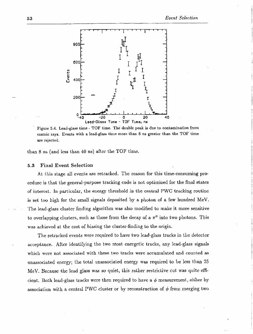
53 Event Selection
200J- -
Lead-Glass Time - TOF Time, ns Figure 5.4. Lead-glass time - TOF time. The double peak is due to contamination from cosmic rays. Events with a lead-glass time more than 8 ns greater than the TOF time are rejected.
than 8 ns (and less than 40 ns) after the TOF time.
5.3 Final Event Selection
.
At this stage all events are retracked. The reason for this time-consuming pro-
cedure is that the general-purpose tracking code is not optimized for the final states
of interest. In particular, the energy threshold in the central PWC tracking routine
is set too high for the small signals deposited by a photon of a few hundred MeV.
The lead-glass cluster finding algorithm was also modified to make it more sensitive
to overlapping clusters, such as those from the decay of a to into two photons. This
was achieved at the cost of biasing the cluster-finding to the origin.
The retracked events were required to have two lead-glass tracks in the detector
acceptance. After identifying the two most energetic tracks, any lead-glass signals
which were not associated with these two tracks were accumulated and counted as
unassociated energy; the total unassociated energy was required to be less than 25
MeV. Because the lead glass was so quiet, this rather restrictive cut was quite effi-
cient. Both lead-glass tracks were then required to have a 4 measurement, either by
association with a central PWC cluster or by reconstruction of 4 from merging two

5.3 Final Event Selection 54
clusters separated by quadrant boundaries.
Next the event was required to be neutral. This was done in a series of cuts, each
more restrictive than the last. To start with, any event with a track in which a lead-
glass cluster was linked to a central-tracker track was rejected. The tracking requires
that the central tracker 6, obtained from charge division, agree with the value of 19
reconstructed in the lead glass. This matching can fail due to mis-measurement in
either system. Because there is such a large background from two-photon production
of charged lepton pairs, -additional check is made for any central tracker hits which
are close to the lead glass track in azimuth. If 3 or more central tracker planes have
hits within 30° in 4, including the first or second plane, the track was classified as - charged. A final criteria was that there be no more than one reconstructed central
tracker track in the event.
Minimum-ionizing tracks were then identified using a careful analysis of layer
energy deposition patterns. The energy in each layer is corrected for attenuation and
a match between the shower shape in the lead glass and the central PWC systems is
required. This cut is aimed primarily at cosmic rays which have evaded all previous
efforts to weed them out, in particular those which pass close to the origin but were
not identified as charged.
The remaining background is mostly from two-photon production of the f2(1270),
a tensor meson which is copiously produced and decays into r”7ro 28% of the time.
The x0’s may appear like two photons if they decay asymmetrically or if the photons
overlap. Shower shape cuts were applied to reduce this background. The lead-glass
shower shape was defined as the second moment of the track, constructed by summing
up the square of the distance of each lead-glass block from the trajectory of the track
in the xz or yz plane, Di, weighted by its energy, Ei:
This quantity was larger for wide showers due to overlapping photons from the decay
of a TO, as seen in fig. 5.5. Both tracks were required to have lead-glass cluster width
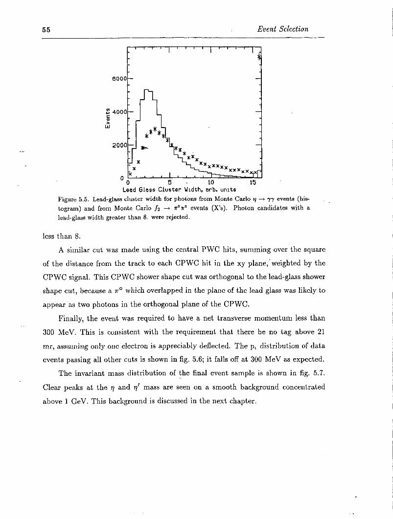
55 Event Selection
I I I I I I I I I I I 1 I I I 1 I I
k
6000- 6000-
:: :: 4000 4000 5 5
15 15 fl fl
***** ***** 2000- 2000- * *
0 -
x X
X I I I 0 5 - 10 15
Lead Glass Cluster Wrdth, arb. units Figure 5.5. Lead-glass cluster width for photbns from Monte Carlo Q + 77 events (his- togram) and from Monte Carlo f2 + TOTO events (X’s). Photon candidates with a lead-glass width greater than 8. were rejected.
less than 8.
A silnilar cut was made using the central PWC hits, summing over the square
of the distance from the track to each CPWC hit in the xy plane,-weighted by the
CPWC signal. This CPWC shower shape cut was orthogonal to the lead-glass shower
shape cut, because a ;ry” which overlapped in the plane of the lead glass was likely to
appear as two photons in the orthogonal plane of the CPWC.
Finally, the event was required to have a net transverse momentum less than
300 MeV. This is consistent with the requirement that there be no tag above 21
mr, assuming only one electron is appreciably deflected. The pt distribution of data
events passing all other cuts is shown in fig. 5.6; it falls off at 300 MeV as expected.
The invariant mass distribution of the final event sample is shown in fig. 5.7.
Clear peaks at the 17 and q’ mass are seen on a smooth background concentrated
above 1 GeV. This background is discussed in the next chapter.
.
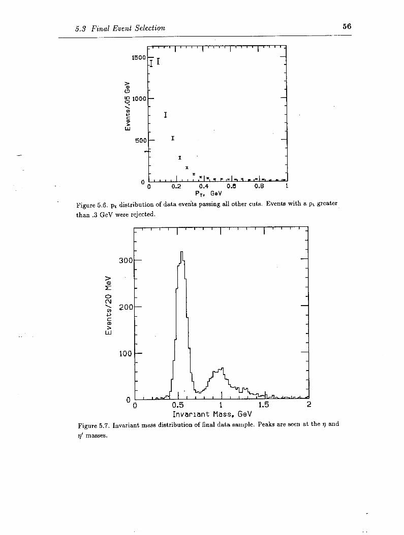
5.3 Final Event Selection 56
P,, Gel’
Figure 5.6. pt distribution of data events passing all other cuts. Events with a pt greater than .3 GeV were rejected.
300
200
100 _,
Invariant Mass, GeV Figure 5.7. Invariant mass distribution of final data sample. Peaks are seen at the q and rj’ masses.
6
Background Calculations
6.1 Sources of Background Events
Events from the decays q + yy and 77’ + yy have a distinctive signature, as
discussed in the introduction to the previous chapter. Background events which can
fake this signature can be divided into two general categories: those which originate
from beam-beam interactions and those which do not. In the former category are
fourth-order QED processes with two photons in the final state, as well as two-photon
production of resonances with decay modes that include photons. Another source of
background could be due to the misidentification of charged particles, in reactions
such as e+e- + (e+e-)e+e-. These processes are all calculable, so it is straightforward
to estimate the background from each one. In the second category are cosmic rays and
beam-gas interactions. We can use the data to estimate the expected contribution
from these sources. The details of all’ background estimates are presented in this
chapter.
6.2 Fourth-Order QED Backgrounds
The QED diagrams which contribute to the process e+e- -+ (e+e-)yy include the
bremsstrahlung diagrams of fig. 6.1 as well as the box diagram of fig. l.la, inserted
into the usual two-photon diagram. (Other diagrams which do not contribute to
the unta,gged topology with both photons at wide angles have been neglected.) The
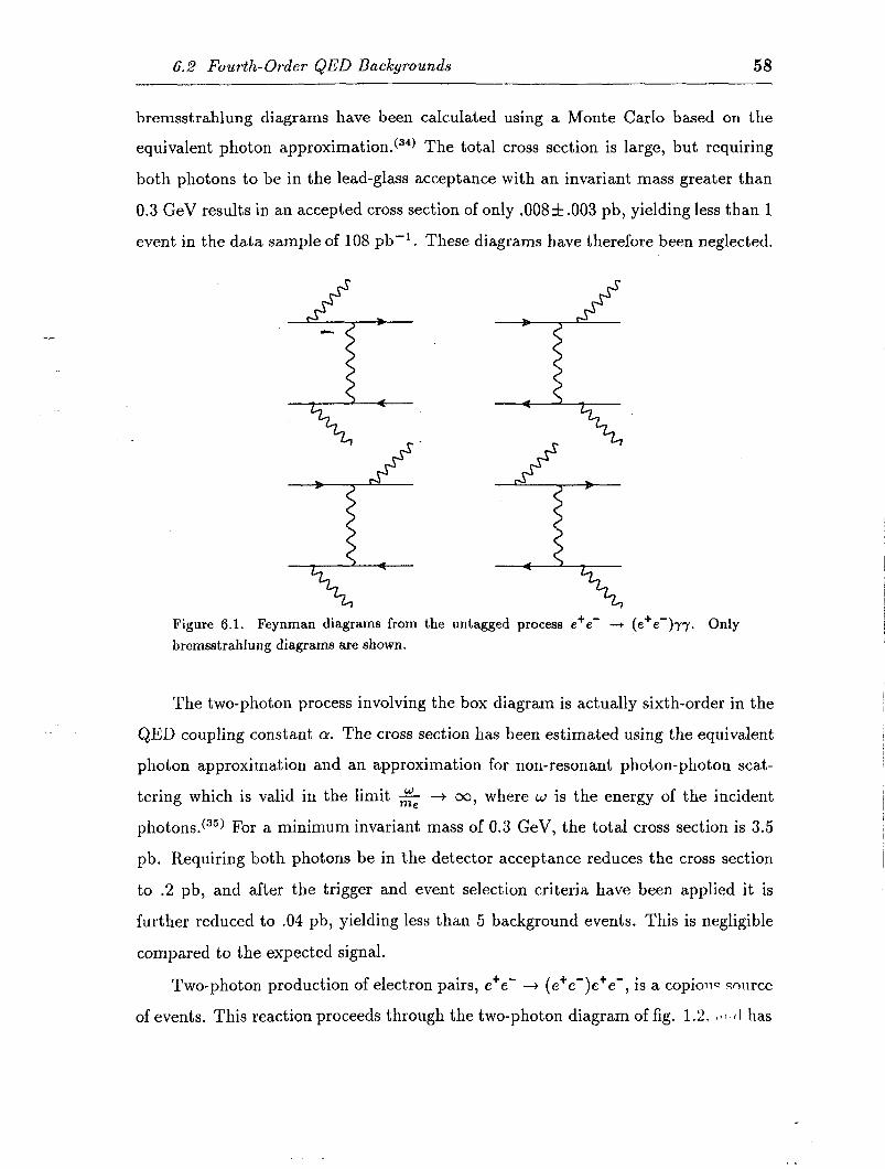
6.2 Fourth-Order QED Backgrounds 58
bremsstrahlung dia.grams have been calculated using a Monte Carlo based on the
equivalent photon approximation. c3*) The total cross section is large, but requiring
both photons to be in the lead-glass acceptance with an invariant mass greater than
0.3 GeV results in an accepted cross section of only .008f.003 pb, yielding less than 1
event in the data sample of 108 pb -‘, These diagrams have therefore been neglected.
Figure 6.1. Feynman diagrams from bremsstrahlung diagrams are shown.
the untagged process e+e- + (e+e-177. Only
The two-photon process involving the box diagram is actually sixth-order in the
QED coupling constant cr. The cross section has been estimated using the equivalent
photon approximation and an approximation for non-resonant photon-photon scat-
tering which is valid in the limit e + 00, where w is the energy of the incident
photons.(35) For a minimum invariant mass of 0.3 GeV, the total cross section is 3.5
pb. Requiring both photons be in the detector acceptance reduces the cross section
to .2 pb, and after the trigger and event selection criteria have been applied it is
further reduced to .04 pb, yielding less than 5 background events. This is negligible
compared to the expected signal.
Two-photon production of electron pairs, e+e- t (e+e-)e+e-, is a copious source
of events. This reaction proceeds through the two-photon diagram of fig. 1.2. ~ll’l has
59 Background Calculations
the same topology as the signal. The only difference is that the events are charged;
otherwise electrons and photons are indistinguishable in the ASP detector.
For charged particle identification we rely on the central tracker, which has five
layers of tracking. To determine the efficiency of the central tracker, cosmic ray events
from the early VS cosmic trigger were used. The penetrating cosmic radiation consists
primarily of muons which should leave charged tracks if they pass through the central
tracker. To identify such events, a track in the calorimeter was required with at least
four layers hit in the central ?WC system, pointing to within 3 cm of the origin in
the transverse plane. This insured that the tracks did indeed pass through the central
tracker and would leave a pattern of hits similar to that from tracks originating from
the origin.
.
To see if the central tracker had registered the track, the azimuthal angle of the
central PWC track was calculated with a constraint to the origin and a search was
made for central tracker tracks which were within f30° in 4. If none was found,
individual central tracker hits within the same angular region were identified, and the
same requirements made in the data analysis were applied to determine if the track
was charged. (At least three hits, with at least one in the first or second layer.) Of
the 19,775 cosmic ray tracks subjected to this test, 78 were found to be neutral. They
were all scanned, and of these 48 were found to be due to central tracker inefficiency.
The others were tracks which did not pass through the central tracker and had been
mis-measured by the central PWC system, or tracks which passed vertically between
central tracker tubes in three of the five layers. (This is not possible for tracks which
originate from the origin.) From this result the calculated central tracker efficiency
is 99.76%.
For an event with two charged tracks to be identified as neutral, the central
tracker would have to fail twice, so the inefficiency for this is .0024’, or .0006%. From
an analysis of e+e- --+ (e+e-)e+e- events in the data, the number of events which
pass all event selection criteria for the ry final state but are identified as charged
is approximately 220,000. Thus the background due to mis-identification of electron
pairs from two-photon interactions is 1.3 events and can be neglected.
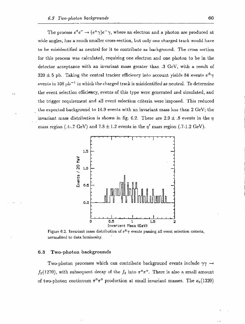
6.3 Two-photon backgrounds 60
The process e+e- + (e+y)e-y, where an electron and a photon are produced at
wide angles, has a much smaller cross-section, but only one charged track would have
to be misidentified as neutral for it to contribute as background. The cross section
for this process was calculated, requiring one electron and one photon to be in the
detector acceptance with an invariant mass greater than .3 GeV, with a result of
320 f 5 pb. Taking the central tracker efficiency into account yields 84 events e*y
events in 108 pb-r in which the charged track is misidentified as neutral. To determine
the event selection efficiency, events of this type were generated and simulated, and
the trigger requirement and all event selection criteria were imposed. This reduced
the expected background to 14.9 events with an invariant mass less than 2 GeV; the
invariant mass distribution is shown in fig. 6.2. There are 2.9 f .8 events in the 17
mass region (.4-.7 GeV) and 7.8 f 1.2 events in the 7’ mass region (.7-1.2 GeV);
1.5
% II 0 c-v 1.0 .
Invariant Mass (GeV) Figure 6.2. Invariant mass distribution of e*y events passing all event selection criteria, normalized to data luminosity. -
6.3 Two-photon backgrounds
Two-photon processes which can contribute background events include yr +
f,(1270), with subsequent decay of the fi into 7r07ro. There is also a small amount
of two-photon continuum ROT’ production at small invariant masses. The ~~(1320)
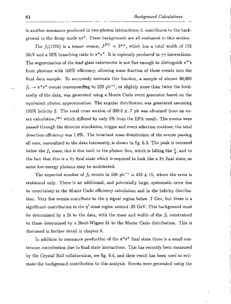
61 Background Calculations
is another resonance produced in two-photon interactions; it contributes to the back-
ground in the decay mode 7~~. These backgrounds are all evaluated in this section.
The f2 (1270) is a tensor meson, Jpc = 2++, which has a total width of 176
MeV and a 28% branching ratio to r”7ro. It is copiously produced in yy interactions.
The segmentation of the lead-glass calorimeter is not fine enough to distinguish TO’S
from photons with 100% efficiency, allowing some fraction of these events into the
final data sample. To accurately estimate this fraction, a sample of almost 90,000
fi 4 7r07ro events corresponding to 220 pb-I, or slightly more than twice the lumi-
nosity of the data, was generated using a Monte Carlo event generator based on the
equivalent photon approximation. The angular distribution was generated assuming
100% helicity 2. The total cross section of 399.5 f .7 pb was obtained from an ex-
act calculation,(36) which differed by only 5% from the EPA result. The events were
passed through the detector simulation, trigger and event selection routines; the total
detection efficiency was 1.0%. The invariant mass distribution of the events passing
all cuts, normalized to the data luminosity, is shown in fig. 6.3. The peak is centered
below the fi mass; this is due both to the photon flux, which is falling like 5, and to
the fact that this is a 41/ final state which is required to look like a 2~ final state, so
some low-energy photons may be undetected.
The expected number of fi events in 108 pb-l is 423 f 15, where the error is
statistical only. There is an additional, and potentially large, systematic error due
to uncertainty in the Monte Carlo efficiency calculation and in the helicity distribu-
tion. Very few events contribute to the 7 signal region below .7 Gev, but there is a
significant contribution to the 7’ mass region around .95 GeV. This background must
be determined by a fit to the data, with the mass and width of the fi constrained
to those determined by a Breit-Wignerfit to the Monte Carlo distribution. This is
discussed in further detail in chapter 8.
In addition to resonance production of the w”xo final state there is a small con-
tinuum contribution due to final state interactions. This has recently been measured
by the Crystal Ball collaboration, see fig. 6.4, and their result has been used to esti-
mate the background contribution to this analysis. Events were generated using the

6.9 Two-photon backgrounds 62
0 0.5 1 1.5 2 Invariant Mass (GeV)
Figure 6.3. Invariant mass distributi& of fz(l270) + a”?ro events passing all event selection criteria, normalized to data luminosity.
equivalent photon approximation and a lookup table for the yy 3 7r07ro cross section
taken from fig. 6.4. Above an invariant mass of .8 GeV the fz(1270) contribution
dominates, so the continuum cross section was assumed to fall like -$, the theoretical
expectation. The events were passed through the detector simulation and the event
selection routines. The total production cross section was 414 pb; 584 pb-l were
generated, more than five times the data luminosity. The invariant mass spectrum
of events passing all cuts is shown in fig. 6.5. The expected number of background
events from this source is estimated to be 44 f 22, 37 of them in the 7 mass region.
An error of 50% has been assigned because of the limited information available on
the shape and magnitude of the continuum yy t wow0 cross section.
To estimate the contribution from the a2(1320), events were generated using the
equivalent photon approximation. A total luminosity of 220 pb-l was generated in
the decay mode a2 + r/r’, the mode most likely to contribute. From this the expected
number of a2 events was determined to be 9 f 2, with an invariant mass distribution
centered near 1.1 GeV. There are no events in the 7 mass region, and a total of 6f 1.7
events in the 7’ mass region.
63 Background Calculations
150 -
100 - 9 c
b’
50 - --
Invariant Mass (MeV)
-Figure 6.4. Invariant mass distribution of ?r”.xo events measured by the Crystal Ball, for events with 1 cosO*l < .8. Continuum production below the fi(1270) resonance is evident.
1 t t I t $1 I I# 1 I # I I I1 0 0.5 1 1.5 2
Invariant Mass (GeV1
Figure 6.5. Invariant mass distribution ofm7r07r0 continuum events passing all cuts.
6.4 Cosmic Rays
Cosmic rays are continually bathing the detector with minimum-ionizing parti-
cles. They are spatially and temporally uncorrelated with the beam crossing, and
most deposit too little energy in the lead-glass calorimeter to trigger the detector.
Yet they are still one of the most persistent and difficult backgrounds.
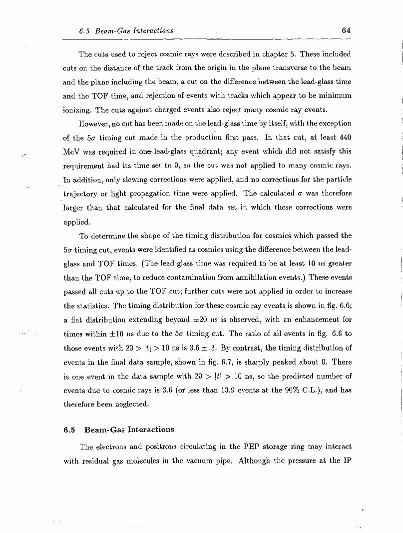
6.5 Beam-Gas Interactions 64
The cuts used to reject cosmic rays were described in chapter 5. These included
cuts on the distance of the track from the origin in the plane transverse to the beam
and the plane including the beam, a cut on the difference between the lead-glass time
and the TOF time, and rejection of events with tracks which appear to be minimum
ionizing. The cuts against charged events also reject many cosmic ray events.
Bowever, no cut has been made on the lead-glass time by itself, with the exception
of the 5a timing cut made in the production first pass. In that cut, at least 440
MeV was required in omlead-glass quadrant; any event which did not satisfy this -
requirement had its time set to 0, so the cut was not applied to many cosmic rays.
In addition, only slewing corrections were applied, and no corrections for the particle - trajectory or light propagation time were applied. The calculated o was therefore
larger than that calculated for the final data set in which these corrections were
applied.
To determine the shape of the timing distribution for cosmics which passed the
50 timing cut, events were identified as cosmics using the difference between the lead-
glass and TOF times. (The lead glass time was required to be at least 10 ns greater
than the TOF time, to reduce contamination from annihilation events.) These events
passed all cuts up to the TOF cut; further cuts were not applied in order to increase
the statistics. The timing distribution for these cosmic ray events is shown in fig. 6.6;
a flat distribution extending beyond f20 ns is observed, with an enhancement for
times within f10 ns due to the 50 timing cut. The ratio of all events in fig. 6.6 to
those events with 20 > ItI > 10 ns is 3.6 f .3. By contrast, the timing distribution of
events in the final data sample, shown in fig. 6.7, is sharply peaked about 0. There
is one event in the data sample with 20 > ItI > 10 ns, so the predicted number of
events due to cosmic rays is 3.6 (or less than 13.9 events at the 90% C.L.), and has
therefore been neglected.
6.5 Beam-Gas Interactions
The electrons and positrons circulating in the PEP storage ring may interact
with residual gas molecules in the vacuum pipe. Although the pressure at the IP

65 Background Calculations
Lead Glass Time, ns
‘Figure 6.6. Event time for cosmic ray events which passed the 5a timing is an artifact of the cut.
cut. The peak
Figure 6.7. Event time for all events in final sample.
500 - I
I
250 -
I I
I o-' " " ' I' " "
I z " " " '-
-20 -10 0 10 20 Lead Glass Trme, ns
was typically lo-’ Torr or less, that works out to 3.2 x lo7 particles per cm3. These
beam-gas collisions typically produce debris at very low angles, but occasionally the
collision products may enter the detector.
A particularly dangerous background comes from photo-production of 71 mesons,
resulting in an invariant mass distribution similar to that of two-photon production
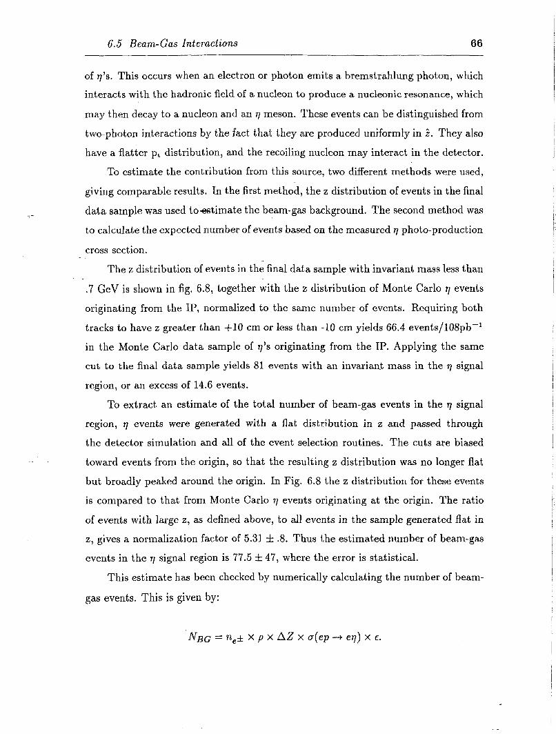
6.5 Beam-Gas Interactions 66
of 7’s. This occurs when an electron or photon emits a bremstrahlung photon, which
interacts with the hadronic field of a nucleon to produce a nucleonic resonance, which
may then decay to a nucleon and an 17 meson. These events can be distinguished from
two-photon interactions by the fact that they are produced uniformly in 2. They also
have a flatter pt distribution, and the recoiling nucleon may interact in the detector.
To estimate the contribution from this source, two different methods were used,
giving comparable results. In the first method, the z distribution of events in the final
data sample was used to-timate the beam-gas background. The second method was
to calculate the expected number of events based on the measured 77 photo-production
cross section.
--.
The z distribution of events in the final data sample with invariant mass less than
.7 GeV is shown in fig. 6.8, together with the z distribution of Monte Carlo q events
originating from the IP, normalized to the same number of events. Requiring both
tracks to have z greater than +lO cm or less than -10 cm yields 66.4 events/l08pb-l
in the Monte Carlo data sample of v’s originating from the IP. Applying the same
cut to the final data sample yields 81 events with an invariant mass in the q signal
region, or an excess of 14.6 events.
To extract an estimate of the total number of beam-gas events in the 7 signal
region, 17 events were generated with a flat distribution in z and passed through
the detector simulation and all of the event selection routines. The cuts are biased
toward events from the origin, so that the resulting z distribution was no longer flat
but broadly peaked around the origin. In Fig. 6.8 the z distribution for these events
is compared to that from Monte Carlo 77 events originating at the origin. The ratio
of events with large z, as defined above, to all events in the sample generated flat in
z, gives a normalization factor of 5.31 f 2. Thus the estimated number of beam-gas
events in the 11 signal region is 77.5 f 47, where the error is statistical.
This estimate has been checked by numerically calculating the number of beam-
gas events. This is given by:
IVBG = n,k x p x AZ x a(ep + er)) x e.
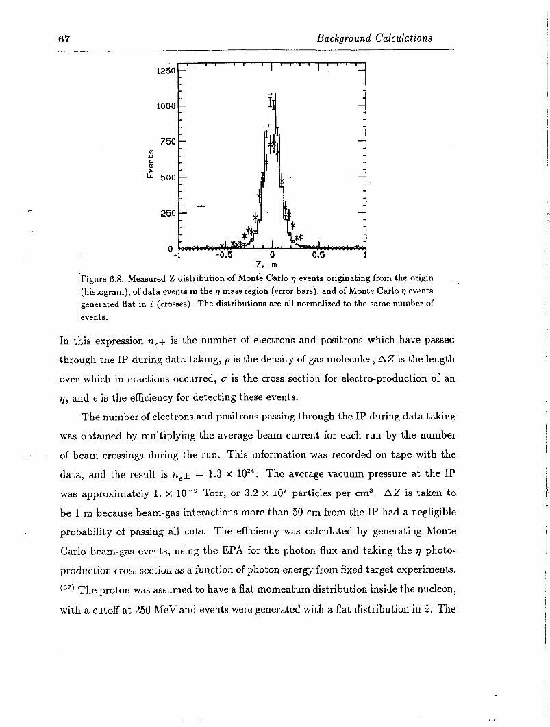
67 Background Calculations
Z, m
-Figure 6.8. Measured Z distribution of Monte Carlo q events originating from the origin (histogram), of data events in the r] mass region (error bars), and of Monte Carlo q events generated flat in f (crosses). The distributions are all normalized to the same number of events.
In this expression n,k is the number of electrons and positrons which have passed
through the IP during data taking, p is the density of gas molecules, AZ is the length
over which interactions occurred, Q is the cross section for electro-production of an
11, and E is the efficiency for detecting these events.
The number of electrons and positrons passing through the IP during data taking
was obtained by multiplying the average beam current for each run by the number
.. of beam crossings during the run. This information was recorded on tape with the
data, and the result is n,k = 1.3 x 10²*. The average vacuum pressure at the IP
was approximately 1. x lo-’ Torr, or 3.2 x lo7 particles per cm3. AZ is taken to
be 1 m because beam-gas interactions more than 50 cm from the IP had a negligible
probability of passing all cuts. The efficiency was calculated by generating Monte
Carlo beam-gas events, using the EPA for the photon flux and taking the 77 photo-
production cross section as a function of photon energy from fixed target experiments.
c3’) The proton was assumed to have a flat momentum distribution inside the nucleon,
with a cutoff at 250 MeV and events were generated with a flat distribution in 2. The
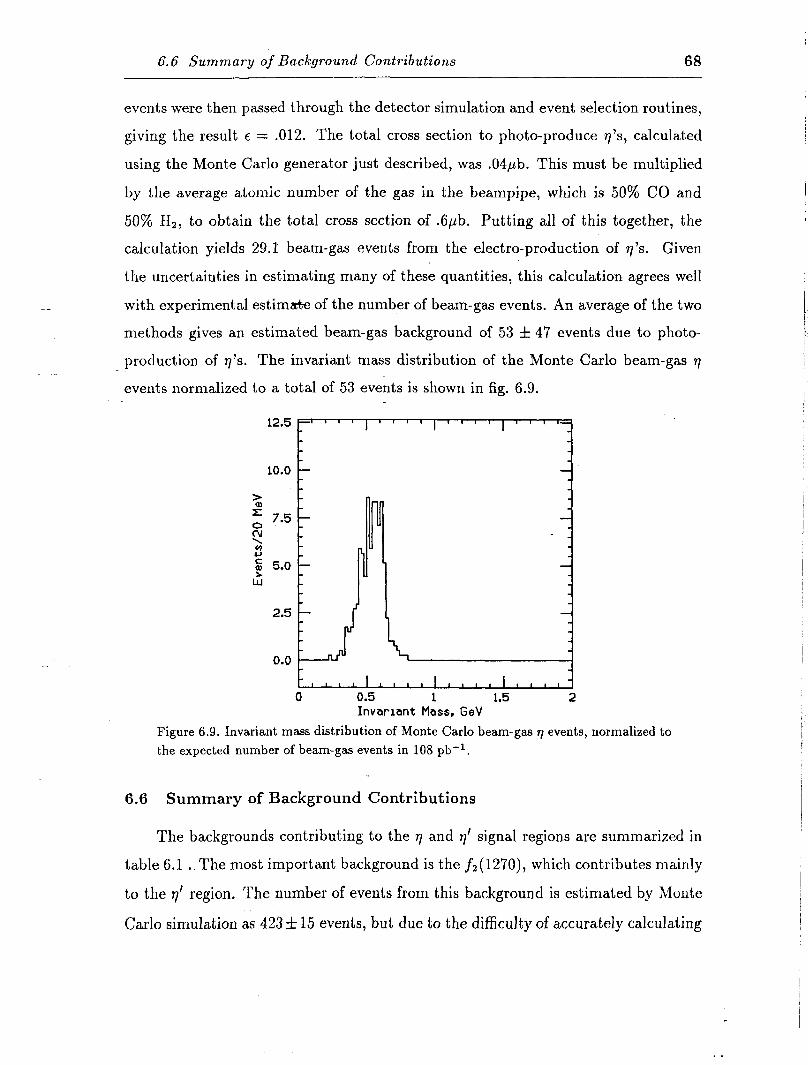
6.6 Summary of Background Contributions 68
events were then passed through the detector simulation and event selection routines,
giving the result c = .012. The total cross section to photo-produce v’s, calculated
using the Monte Carlo generator just described, was .04pb. This must be multiplied
by the average atomic number of the gas in the beampipe, which is 50% CO and
50% 112, to obtain the total cross section of .6pb. Putting all of this together, the
calculation yields 29.1: beam-gas events from the electro-production of 7’s. Given
the uncertainties in estimating many of these quantities, this calculation agrees well
with experimental estimate of the number of beam-gas events. An average of the two
methods gives an estimated beam-gas background of 53 f 47 events due to photo-
production of 77’s. The invariant mass distribution of the Monte Carlo beam-gas 77
-
events normalized to a total of 53 events is shown in fig. 6.9.
12.5
10.0
2.5
0.0
Figure 6.9. Invariant mass distribution of Monte Carlo beam-gas q events, normalized to the expected number of beam-gas events in 108 pb-l.
6.6 Summary of Background Contributions
The backgrounds contributing to the q and 77’ signal regions are summarized in
table 6.1 . The most important background is the f2(1270), which contributes mainly
to the 7’ region. The number of events from this background is estimated by Monte
Carlo simulation as 423 f 15 events, but due to the difficulty of accurately calculating

69 Background Calculations
the detection efficiency for very low-energy photons (< 100 MeV) it is more accurate
to fit the data. This will be done in chapter 8.
Table 6.1. Background contributions to the 7 mass region (.4-.7 GeV) and to the 9’ mass region (.7-1.2 GeV).
Process I 7 Region I 9’ Region
ef7 ( 2.9f.8 ( 7.8f1.2
f2 --O” -+7r R Id etermined from fit to dat;
yy -+ 7r”ro continuum 1 37f19 1 7f3
a2 + yr" 0 6 f 1.7
Beam-gas 53 f 47 0
Total - f2 ] 92.9 f 50.7 1 13.8 f 2.1
Backgrounds which contribute to v region are small; the only significant ones are
from continuum two-photon r”7ro production and from beam-gas production of q’s
Unfortunately the systematic errors on both of these backgrounds are large due to
the dificulty of estimating them, but fortunately they are small backgrounds. They
will be subtracted from the number of 77 events which will be determined by fitting
the data in chapter 8.

7
Efficiency Calculations
The efficiency to detect an event .of the type 77 + ry or 7’ -+ y-y is defined as the
ratio of events detected to the total which are produced. This definition includes the
detector acceptance, the trigger efficiency, and the event selection efficiencies. The
effic.iencies are calculated sequentially, i.e. the efficiency for a cut is based on the
number of events which passed all previous cuts.
The event simulation routines described in chapter 4 have been used extensively
in these calculations. Events were generated using the Monte Carlo method described
in section 4.1, then passed through the event simulation routines. The resulting Monte
Carlo ‘data’ is then analyzed in exactly the same way as the real data. The fraction
of Monte Carlo events which are in the detector acceptance, satisfy the trigger and
pass all of the event selection criteria (described in chapter 5) gives the efficiency.
It is important to know not only the efficiency, but also the errors associated
with these calculations. The statistical errors are small because the Monte Carlo
event samples are large. Almost 400,000 77 -+ yy and 25,000 r]’ --+ yy events were
generated, corresponding to a luminosity seven times greater than the data. The
systematic errors can be important in some cases. Both the efficiency calculations
and the error analysis are presented in this chapter.
The luminosity measurement concludes this chapter. The luminosity, 6, together
with the observed number of events, N, and the efficiency, c, gives the radiative width
71 Eficiency Calculations
according:
rx - N
YY - - a.lec.Br(X -+ 77)’ (7.1)
In this expression, 3 is the production cross section assuming I’$, = 1 keV, as dis-
cussed in chapter 4, and Br(X + 77) is the branching ratio into two photons, which
in the case of the 7 and 7’ is known from fixed target experiments.
7.1 Detector AcceptancL -
Both photons from the decay of an ‘7 or 77’ must be within the sensitive part of the
lead-glass calorimeter, delined as 20’ < 8, < 160’ (for the definition of 0, see section
5.2). The detector acceptance is calculated using the Monte Carlo generated samples
of q --$ yy and 7’ -t yy events, which were passed through the same tracking routines
applied to the data. The events were required to have at least two reconstructed lead-
glass clusters with an energy greater than 100 MeV and 20’ < 8, < 160°.
In addition, for the event to be classified as untagged the outgoing electrons had
to be within 21 mr of the beamline. The fraction of untagged events was determined
without any detector simulation, by simply calculating the trajectory of the outgoing
electrons in each Monte Carlo event. The position of the interaction point, generated
with a gaussian distribution about the measured beamspot, was taken into account
in this calculation.
The results of the acceptance calculations are summarized in table 7.1 . The
combined detector acceptance, which includes the calorimeter acceptance and the
tagging veto, was 25.9% for q events and 29.4% for 77’ events.
Table 7.1. Detector acceptance for 17 and $ events.
rl 7’
Lead Glass Acceptance 30.7 f 0.6% 37.2 f 0.6%
No Tag 84.3 f 0.6% 82.3 f 0.6%
Combined Acceptance 25.9 f 0.5% 30.6 f 0.5% I 1
7.1 Detector Acceptance 72
-
The systematic error associated with these calculations depends on how accu-
rately the geometry constants are known. The geometry of the lead-glass calorimeter
was determined by an iterative method. For the starting point, the position of each
lead-glass block was measured with a ruler. Through-going cosmic rays were then
used to calculate residuals for each block, and the constants were adjusted to mini-
mize the residuals. This process was repeated until no further improvement could be
obtained; the error was estimated to be no more than a few mm on the position of
each block. These geometry constants were used in the Monte Carlo data simulation.
To check the accuracy of the geometry constants we can compare the 6 distribu-
tions of the data with the Monte Carlo, using two data samples. The first is the q
data, in the invariant mass region from 0.4 to 0.7 GeV where there is little background.
This comparison is shown in fig. 7.1; the points are the data and the histogram is
the Monte Carlo normalized to the same number of events. Fairly good agreement is
observed, but the statistical errors are too large for a precise comparison.
Theta, Deqrees
Figure 7.1. 0 distribution of y events passing all event selection criteria. The the points, the histogram is the Monte Carlo simulation normalized to number in the data.
data are of events
For higher statistics we turn to another data sample, the untagged QED process
e+e- + (e+e-)e+e-. Because these ‘e-pair’ events are primarily produced through a

73 Eficiency Calculations
two-photon like diagram, they are very similar to the 7 and 7’ data samples; the final
state consists of two lead-glass clusters back-to-back in the azimuthal plane, with a
forward-peaked 6’ distribution.
Untagged events from the process e+e- + (e+e-)e+e- were written out together
with 77 and 7’ events by the first pass filter. The charged events were then separated
from the neutral events by a different set of final event selection criteria. The main
difference was that both tracks were required to be charged rather than neutral.
Several cuts which were applied to the neutral events were not applied to the e-pairs.
The software trigger cut was not applied. Also, because the central tracker provides
a $ measurement for charged tracks, the e-pairs were not required to have a central
PWC 4 measurement. The shower shape cuts were not applied to the e-pairs, and
the requirement that A# 2 135’ was also omitted. The stray energy cut was set
to 50 MeV, rather than the more stringent 25 MeV cut applied to the neutral data.
Finally, the acceptance for e-pairs was 30’ < 8, < 150° rather than 20’ 5 0, 5 160°.
(This was simply because of an error in generating the Monte Carlo data sample; due
to the large amount of CPU time necessary to generate the Monte Carlo sample, it
was more expedient to change the acceptance.) Other than these cuts which were
omitted or modified, the selection procedure for e-pairs was identical to that for the
yy data sample.
The data sample of e-pairs consisted of approximately 220,000 events; a Monte
Carlo sample corresponding to about one-third the luminosity of the data was also
generated, using the AX0 computer program(38) modified to generate unweighted
events. This routine was checked against an exact Monte Carlo event generator
and found to be in excellent agreement. t3’) The Monte Carlo events were simulated,
tracked and passed through the same event selection routines. Using only the lead-
glass information to calculate 19 (and ignoring the central tracker information), the
8 distributions for data and Monte Carlo shown in fig. 7.2 were obtained. Excellent
agreement is observed.
In both the 77 data and the e-pair data the B distributions are not smooth, but
7.2 Trigger E’ciency
30001
74
Theta, Dsqrees
Figure 7.2. 0 distribution of e-pair events. The data are the points, the histogram is the Monte Carlo simulation normalized to number of events in the data.
ragged, reflecting the granularity of the lead-glass calorimeter (each block is 6x6
cm). The good agreement between the data (representing the ‘true’ geometry) and
the Monte Carlo (the calculated geometry) shows that the geometry constants are
accurate to better than lo at 90”, corresponding to an error in block position of 3.2
mm. The uncertainty in angle at the 20° cutoff is f.l2O, resulting in an uncertainty
in the lead-glass acceptance of 0.6%.
The forward tag veto at 21 mr from the beamline was defined by a tungsten
mask in the beampipe. Assuming that the position of the veto is accurate to within
1 mr results in an error of .6% in the no-tag acceptance.
The combined error is obtained by adding the systematic errors in quadrature,
since the lead-glass geometry and the beam-pipe geometry are assumed to have in-
dependent errors. The results are given in table 7.1.
7.2 Trigger Efficiency
We have previously noted that the lowest threshold of the lead-glass trigger was
approximately .7 GeV, so the trigger efficiency for q’s (M=.549 GeV) will obviously
not be 100%. For the 7’ (M=.957 GeV) the situation is much better and the trigger
75 Eficiency Calculations
efficiency is close to 100%.
To calculate the trigger efficiency we rely on the detailed trigger simulation de-
scribed in section 4.3. The event simulation routines produce the raw signal from
each PMT, including,the effects of PMT gain and attenuation in the lead glass. The
trigger logic is then applied to the raw signals, including threshold effects. The trigger
efficiency for 77 events which are in the detector acceptance is 47.9%, and for 7’ events
it is 95.0%. In order to eliminate the threshold region where the trigger efficiency
is changing rapidly, a ‘softwibpe trigger’ cut at 2400 counts has been introduced, as
discussed in chapter 5. This restricts the acceptance to a region where the trigger
efficiency is high and fairly flat. The efficiency for the combined hardware and soft-
ware triggers is 40.9% on r,~ events and 94.7% on q’ events. At the cost of a small loss
in efficiency we have eliminated a region which contributes a significant systematic’
/
I
error.
The systematic error on the trigger requirement has several sources. Uncertainty
in the energy scale of the Monte Carlo introduces an error in the number of events
passing both the software trigger and the hardware trigger. Like-wise, uncertainty
in the energy resolution introduces an error because of smearing effects. Finally,
inaccuracies in the hardware trigger simulation may result in an additional systematic
error.
The energy scale and resolution were originally determined using kinematically
. fit radiative Bhabhas, as described in section 3.2, and the Monte Carlo scale was
determined by requiring the simulated energy to agree with the data using the method
described in section 4.2. The 7 peak provides an excellent means of measuring both
the energy scale and resolution, and provides a check of the agreement between data
and Monte Carlo simulation.
A fit to the entire data set and to the 84/85 and 85/86 data cycles individually
gives the results shown in table 7.2 . There is a shift of 1.1% between the first and
second cycles, which can be attributed to the fact that the lead-glass calibration
constants were determined separately for the two data cycles. (Fits to smaller data
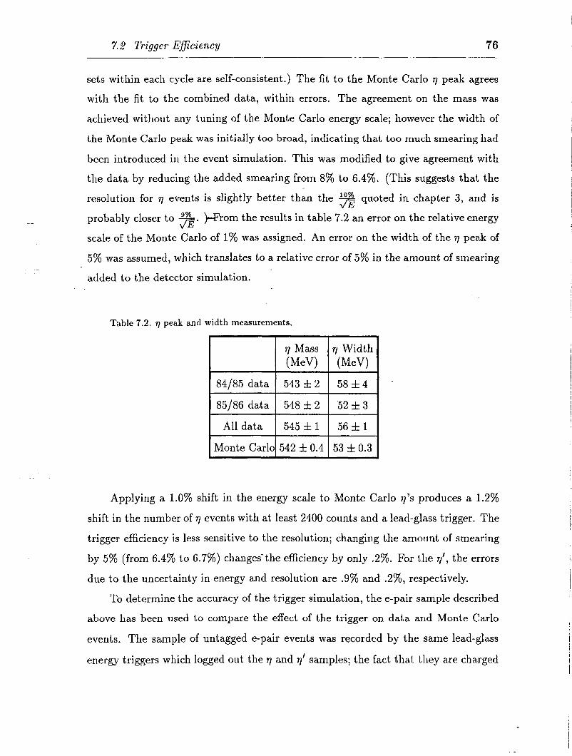
7.2 Trigger Efficiency 76
sets within each cycle are self-consistent.) The fit to the Monte Carlo n peak agrees
with the fit to the combined data, within errors. The agreement on the mass was
achieved without any tuning of the Monte Carlo energy scale; however the width of
the Monte Carlo peak was initially too broad, indicating that too much smearing had
been introduced in the event simulation. This was modified to give agreement with
the data by reducing the added smearing from 8% to 6.4%. (This suggests that the
resolution for 77 events is slightly better than the s quoted in chapter 3, and is
probably closer to 3. prom the results in table 7.2 an error on the relative energy
scale of the Monte Carlo of 1% was assigned. An error on the width of the 7 peak of
5% was assumed, which translates to a relative error of 5% in the amount of smearing
added to the detector simulation.
--
Table 7.2. 17 peak and width measurements.
Applying a 1.0% shift in the energy scale to Monte Carlo 7’s produces a 1.2%
shift in the number of q events with at least 2400 counts and a lead-glass trigger. The
trigger efficiency is less sensitive to the resolution; changing the amount of smearing
by 5% (from 6.4% to 6.7%) changes‘.the efficiency by only .2%. For the q’, the errors
due to the uncertainty in energy and resolution are .9% and .2%, respectively.
To determine the accuracy of the trigger simulation, the e-pair sample described
above has been used to compare the effect of the trigger on data and Monte Carlo
events. The sample of untagged e-pair events was recorded by the same lead-glass
energy triggers which logged out the 17 and 7’ samples; the fact that they are charged

77 Eficiency Calculations
does not affect the trigger efficiency. * The trigger simulation was applied to the
Monte Carlo e-pair sample; requiring a lead-glass trigger produced the total lead-
glass energy distribution shown as a histogram in fig. 7.3; the data are represented by
error bars. The Monte Carlo data is absolutely normalized to the luminosity of the
data in this plot (determined with low-angle Bhabha events; see section 7.6) and the
software trigger cut has not been applied. On the log scale, the agreement between
data and Monte Carlo in the region 1.5-3.5 GeV is evident. This region is well above
the trigger threshold, and can-be used to check the low-angle Bhabha normalization;
the result agrees to within 1.8%.
Total Enerqy, GeV Total Enerqy, GeV
Figure 7.3. Comparison of Monte Carlo and data energy distributions for e-pair events. All events have a lead-glass trigger but the software trigger cut has not been applied.
The rise of events with decreasing energy is due to both the $ spectrum of the
two-photon process and the i dependence of the ry -+ e+e- cross section. The trigger,
by requiring a minimum deposited energy in the lead-glass calorimeter, produces the
* The super-trigger is vetoed if 3 or more of the central VS scintillators fired. The
inefficiency due to this veto on e-pairs was determined to be negligible by studying
events logged out by a diagnostic trigger, a pre-scaled version of the super-trigger
without any vetos.
7.3 Production First Pass Eficiency 78
observed cut-off in the energy distribution. The comparison between data and Monte
Carlo shows that the trigger simulation reproduces the actual trigger response fairly
well. The ratio of Monte Carlo events to data gives the ratio of the simulated trigger
efficiency to the actual trigger efficiency, bin by bin. From this and the measured
trigger efficiency as a function of energy (fig. 2.7), a quantitative estimate of the
uncertainty in the number of 77 events due to inaccuracies
given by: nbins
in the trigger simulation is
- - AN= x(1- i=l
g)eiNiy
where g is the ratio of Monte Carlo events to data in a given bin, ci is the trigger
(7.2)
efficiency in that bin, and Ni is the number of 77 events per bin before the hardware
trigger is applied (but after the software trigger is applied). The result, using a bin
size of 100 MeV, is an uncertainty of 2.1% due to inaccuracy in the trigger simulation
for 7 events; for 77’ events the uncertainty is only .5%. The quoted uncertainty is
a worst case; the efCects of changing the energy scale or normalization within their
quoted errors is included.
Combining all systematic errors in quadrature yields a trigger efficiency of 40.9f
2.43% for q events and 94.7 f 1.10% for 77’ events.
7.3 Production First Pass Efficiency
The efficiency of the production first pass on 7 and 7’ events which were in the
detector acceptance and passed the trigger requirement was very high, 98.5% and
99.4% respectively. The efficiency of these cuts has been determined by Monte Carlo
simulation. This method is very accurate for all but the timing cut. The lead-glass
time was required to be within 5a “of the beam crossing. No timing information is
included in the event sirnulation, so the efficiency of this cut is estimated using another
data set. The radiative Bhabha event sample is suitable because no timing cut was
made in selecting these events and there is no background from cosmic rays. The
fraction of these events which pass the 5a timing cut is greater than 9!).!)!)%0; therefore
we can neglect any inefficiency from this cut. The individual cuts and efficiencies for
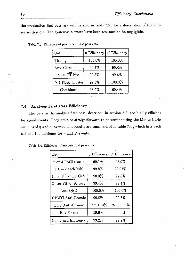
79 Eficiency Calculations
the production first pass are summarized in table 7.3 ; for a description of the cuts
see section 5.1. The systematic errors have been assumed to be negligible.
Table 7.3. Efficiency of production first pass cuts.
cut q Efficiency 7’ Efficiency
Timing 100.0% 100.0%
Anti-Cosmic 99.7% 99.8%
< 80 CT hits 99.3% 99.6%
2 1 PbGl Cluster 99.5% 100.0%
Combined 98.5% 99.4%
7.4 Analysis First Pass Efficiency
The cuts in the analysis first pass, described in section 5.2, are highly efficient
for signal events. They are also straightforward to determine using the Monte Carlo
samples of q and 7’ events. The results are summarized in table 7.4, which lists each
cut and the efficiency for 77 and 77’ events.
Table 7.4. Efficiency of analysis first pass cuts.

7.5 Final Event Selection Eficiency 80
The only cut which cannot be evaluated using the Monte Carlo data samples
is the TOF anti-cosmic cut, because neither the time-of-flight counters nor the lead-
glass timing was included in the Monte Carlo simulation. The efficiency of this cut
has therefore been evaluated using the radiative Bhabha sample. Events with the
e+e-y topology were chosen with one electron or photon in the lead-glass acceptance.
The probability for the event to fail the TOF cut was determined as a function of the
energy and polar angle of the track in the lead-glass calorimeter. This probability
-- was then integrated over-the energy and angular distributions of both tracks in the 7
and 71’ Monte Carlo samples. From this analysis the efficiency for the TOF cut was
determined to be 97.2 f .3% for ‘7 events and 97.0 f .3% for 7’ events, where the error
is clue to the statistical uncertainty of the radiative Bhabha sample. The combined
efficiency of all cuts in the analysis first pass is 93.2% for 77 events and 92.9% for 7’
events. The systematic errors have been assumed to be negligible.
7.5 Final Event Selection Efficiency
The production and analysis first pass filters have a very high combined efficiency
for 7 and 7’ events, as the preceding sections have shown. In the final event selection
several cuts are made with efficiencies in the SO-90% range; these cuts are necessary
to reject the backgrounds discussed in chapter 6. The result is a combined efficiency
for the final event selection criteria of about 50% for both the 77 and q’ event samples.
The efficiencies of the final analysis cuts as determined by Monte Carlo simulation
are displayed in table 7.5 .
The corrections listed in table 7.5 are due to small differences between simulated
events and real events. In particular, the efficiencies for both tracks to have a $
measurement, to be neutral and to pass the stray energy and shower shape cuts
depend on the details of the Monte Carlo simulation of the central PWC’s, the central
tracker and the lead-glass calorimeter. These differences have been estimated using
the radiative Bhabha sample, resulting in the correction factors shown in table 7.5.
These correction factors, and the associated systematic errors, have been calculated
in the manner described below.
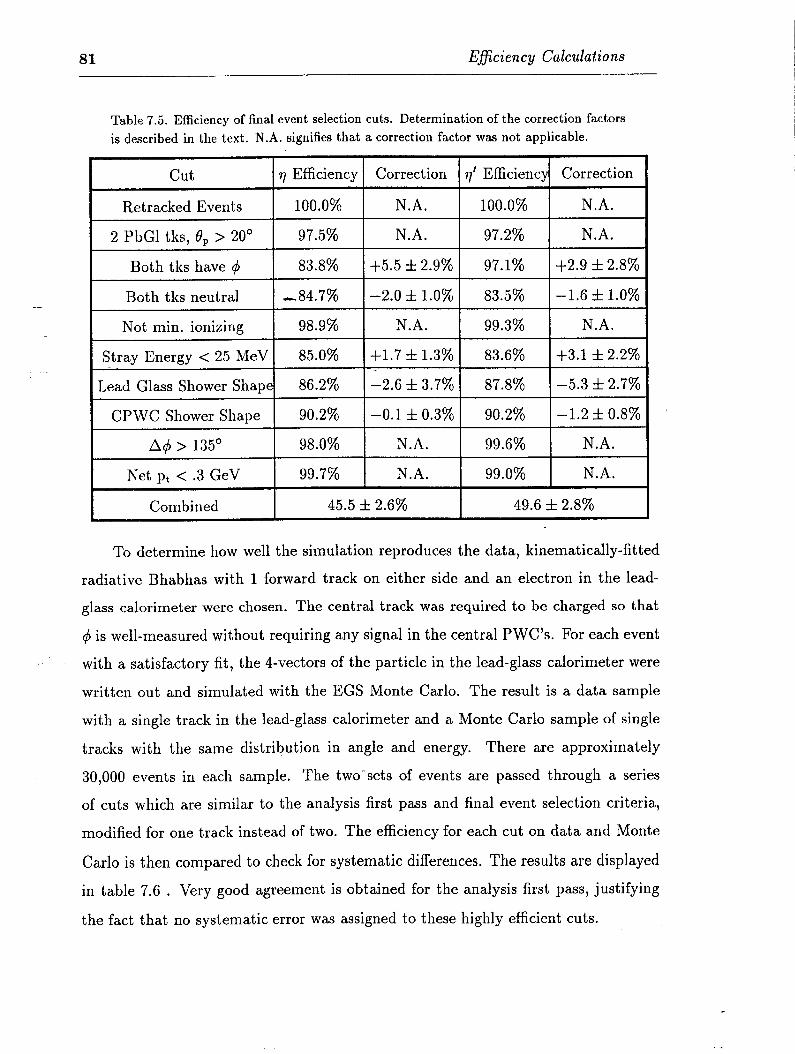
81 Eficiency Calculations
Table 7.5. Efficiency of final event selection cuts. Determination of the correction factors is described in the text. N.A. signifies that a correction factor was not applicable.
cut I 17 Efficiency 1 Correction 17’ Efficiencd Correction
Retracked Events
2 PbGl tks, 6, > 20’
Both tks have 4
100.0% N.A. 100.0% N.A.
97.5% N.A. 97.2% N.A.
83.8% +5.5 d/2.9% 97.1% +2.9 f 2.8%
Both tks neutral 1 -84.7% I-2.0 f 1.0% 1 83.5% 1 -1.6 f 1.0%
Not min. ionizing
Stray Energy < 25 MeV
98.9% N.A. 99.3% N.A.
85.0% +1.7 f 1.3% 83.6% $3.1 f 2.2%
Lead Glass Shower Shape 1 86.2% I-2.6 f 3.7% 1 87.8% 1 -5.3 f 2.7%
CPWC Shower Shape
Ac$ > 135’
90.2% -0.1 f 0.3% 90.2% -1.2 f 0.8%
98.0% N.A. 99.6% N.A.
Net pt < .3 GeV
Combined
99.7% N.A. 99.0% N.A.
45.5 f 2.6% 49.6 f 2.8%
To determine how well the simulation reproduces the data, kinematically-fitted
radiative Bhabhas with 1 forward track on either side and an electron in the lead-
glass calorimeter were chosen. The central track was required to be charged so that
4 is well-measured without requiring any signal in the central PWC’s. For each event
.. with a satisfactory fit, the 4-vectors of the particle in the lead-glass calorimeter were
written out and simulated with the EGS Monte Carlo. The result is a data sample
with a single track in the lead-glass calorimeter and a Monte Carlo sample of single
tracks with the same distribution in angle and energy. There are approximately
30,000 events in each sample. The two-sets of events are passed through a series
of cuts which are similar to the analysis first pass and final event selection criteria,
modified for one track instead of two. The efficiency for each cut on data and Monte
Carlo is then compared to check for systematic differences, The results are displayed
in table 7.6 . Very good agreement is obtained for the analysis first pass, justifying
the fact that no systematic error was assigned to these highly efficient cuts.
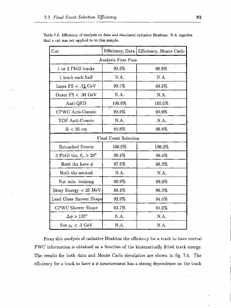
7’.5 Final Event Selection Eficiency 82
Table 7.6. Efficiency of analysis on data and simulated radiative Bhabhas. N.A. signifies that a cut was not applied to to this sample.
cut Efficiency, Data Efficiency, Monte Carlo
Analysis First Pass
1 or 2 PbGl tracks 99.3% 98.9%
1 track each half N.A. N.A.
Inner FS < .lAGeV 99.1% 99.3%
Outer FS < .30 GeV N.A. N.A.
Anti-QED 100.0% 100.0%
CPWC Anti-Cosmic - 99.9% 99.9%
TOF Anti-Cosmic N.A. N.A.
R < 30 cm 99.8% 99.8%
Final Event Selection
Retracked Events 100.0% 100.0%
2 PbGl tks, 8, > 20° 99.4% 99.4%
Both tks have 4 97.5% 96.2%
Both tks neutral N.A. N.A.
Not min. ionizing 99.9% 99.9%
Stray Energy < 25 MeV 88.4% 86.2%
Lead Glass Shower Shape 92.9% 94.8%
CPWC Shower Shape 93.7% 94.8%
A$ > 135’ N.A. N.A.
Net pt < .3 GeV - N.A. N.A. A
Frown this analysis of radiative Bhabhas the efficiency for a track to have central
PWC information is obtained as a function of the kinematically fitted track energy.
The results for both data and Monte Carlo simulation are shown in fig. 7.4. The
efficiency for a track to have a 4 measurement has a strong dependence on the track
.

83 Eficiency Calcdations
energy, rising to 100% in 800 MeV. The Monte Carlo efficiency is systematically
slightly lower. To correct for, this, the difference in efficiencies for data and Monte
Carlo were folded with t;he energy and angular distribution of photons from the 77 and
7’ samples. For 77 events a correction of +5.5 f 2.97 o was calculated, and for 17’ events
the correction is +2.9 f 2.8%. The error is due to statistical uncertainty.
0.8 0.8
c 2
2 0.6
B
b 0.4
1.0 1.0
0.2 0.2
0.0 0.0 0 0 0.5 0.5 1 1 1.5 1.5 2 2 2.5 2.5 3 - 3 -
Track Enerqy, GeV Track Enerqy, GeV
Figure 7.4. Efficiency for a qS measurement from the central PWC system as a function of Figure 7.4. Efficiency for a 4 measurement from the central PWC system as a function of track energy. The error bars are the data and the histogram is Monte Carlo simulation. track energy. The error bars are the data and the histogram is Monte Carlo simulation.
.
The next cut, the requirement that both tracks be neutral, was studied using a
different method. The probability for a photon to convert in a medium with a depth
of X radiation lengths is given by 1 - e-7X/g. At a polar angle of 90’ in the ASP
detector, a photon traverses approximately .063 radiation lengths of beampipe and
central tracker material before entering the lead-glass calorimeter, so the conversion
probability is 4.7%. For events with two photons, integrated over the angular dis-
tribution of photons in the 77 Monte Carlo sample, the probability that at least one
will convert is about 15%. To check this calculation, which was performed with the
EGS Monte Carlo, a comparison of the Monte Carlo with data has been performed
using the process e+e- + yy. Events of this type in which one photon converted
in the beampipe or the central tracker were selected from the data, and the number
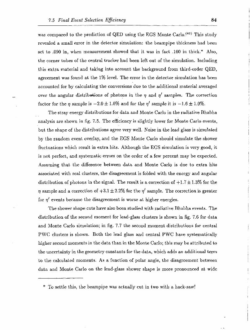
7.5 Final Event Selection Ejiciency 84
was compared to the prediction of QED using the EGS Monte Carlo.(40) This study
revealed a small error in the detector simulation: the beampipe thickness had been
set to .090 in, when measurement showed that it was in fact .lOO in thick.* Also,
the corner tubes of the central tracker had been left out of the simulation. Including
this extra material and taking into account the background from third-order QED,
agreement was found at the 1% level. The error in the detector simulation has been
accounted for by calculating the conversions due to the additional material averaged
over the angular distribdions of photons in the 77 and 7’ samples. The correction
factor for the 17 sample is -2.0 f 1.0% and for the 7’ sample it is -1.6 f 1.0%.
The stray energy distributions for data and Monte Carlo in the radiative Bhabha - analysis are shown in fig. 7.5. The efficiency is slightly lower for Monte Carlo events,
.but the shape of the distributions agree very well. Noise in the lead glass is simulated
by the random event overlay, and the EGS Monte Carlo should simulate the shower
fluctuations which result in extra hits. Although the EGS simulation is very good, it
is not perfect, and systematic errors on the order of a few percent may be expected.
Assuming that the difference between data and Monte Carlo is due to extra hits
associated with real clusters, the disagreement is folded with the energy and angular
distribution of photons in the signal. The result is a correction of $1.7 f 1.3% for the
77 sample and a correction of +3.1 f 2.2% for the 7’ sample. The correction is greater
for q’ events because the disagreement is worse at higher energies.
The shower sha,pe cuts have also been studied with radiative Bhabha events. The
distribution of the second moment for lead-glass clusters is shown in fig. 7.6 for data
and Monte Carlo simulation; in fig. 7.7 the second moment distributions for central
PWC clusters is shown. Both the lead glass and central PWC have systematically
higher second moments in the data than in the Monte Carlo; this may be attributed to
the uncertainty in the geometry constants for the data, which adds an additional term
to the calculated moments. As a function of polar angle, the disagreement between
data and Monte Carlo on the lead-glass shower shape is more pronounced at wide
* To settle this, the beampipe was actually cut in two with a hack-saw!
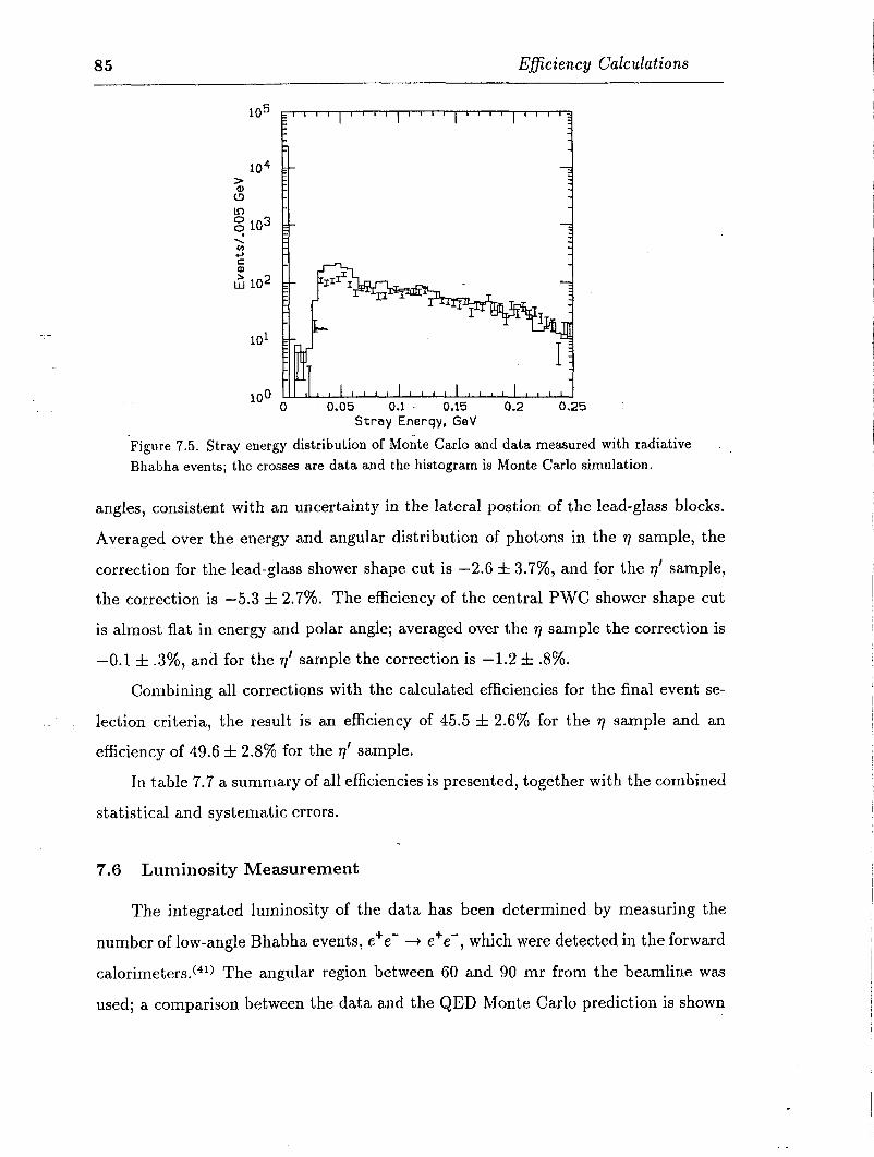
85 Eficiency Calculations
104 > iti
z 0 103 < 3 z Is 102
-
Stray Enerqy, GeV
‘Figure 7.5. Stray energy distribution of Monte Carlo and data measured with radiative Bhabha events; the crosses are data and the histogram is Monte Carlo simulation.
angles, consistent with an uncertainty in the lateral postion of the lead-glass blocks.
Averaged over the energy and angular distribution of photons in the 77 sample, the
correction for the lead-glass shower shape cut is -2.6 f 3.7%, and for the 7’ sample,
the correction is -5.3 f 2.7%. The efficiency of the central PWC shower shape cut
is almost flat in energy and polar angle; averaged over the q sample the correction is
-0.1 f .3%, and for the 7’ sample the correction is -1.2 f .8%.
Combining all corrections with the calculated efficiencies for the final event se-
lection criteria, the result is an efficiency of 45.5 f 2.6% for the 77 sample and an
efficiency of 49.6 f 2.8% for the q’ sample.
In table 7.7 a summary of all efficiencies is presented, together with the combined
statistical and systematic errors.
7.6 Luminosity Measurement
The integrated luminosity of the data has been determined by measuring the
number of low-angle Bhsbha events, e+e- -+ e+e-, which were detected in the forward
calorimeters.(41) The angular region between 60 and 90 mr from the beamline was
used; a comparison between the data and the QED Monte Carlo prediction is shown
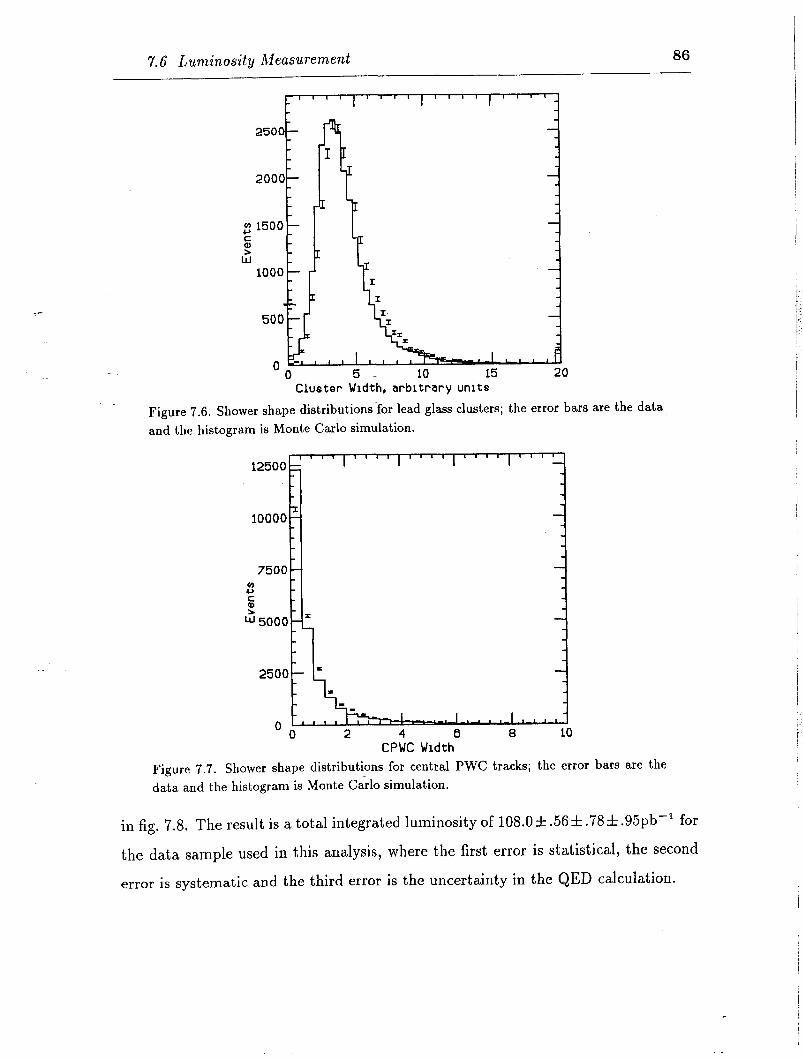
7.6 Luminosity Measurement
Cluster Width, arbitrary units
Figure 7.6. Shower shape distributions‘for lead glass clusters; the error bars are the data and the histogram is Monte Carlo simulation.
-I 10000 -
7500-
3 s
135000--
2500- =
" ' * .-, " " " " " I 4 6 8 10
CPWC Width
Figure 7.7. Shower shape distributions for central PWC tracks; the error bars are the data and the histogram is Monte Carlo simulation.
in fig. 7.8. The result is a total integrated luminosity of 108.0 f .56 f .78f .95pbv1 for
the data sample used in this analysis, where the first error is statistical, the second
error is systematic and the third error is the uncertainty in the QED calculation.
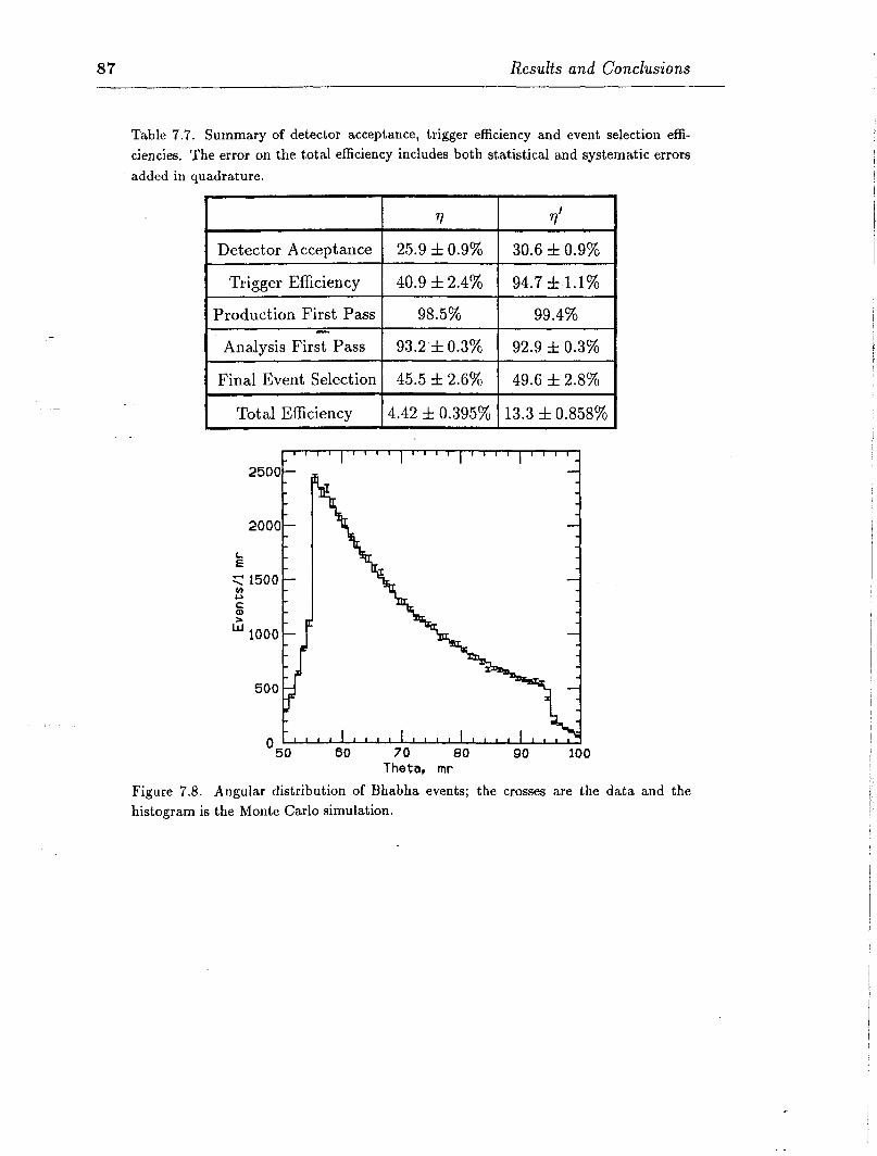
-
87 Results and Conclusions
Table 7.7. Summary of detector acceptance, trigger efficiency and event selection effi- ciencies. The error on the total efficiency includes both statistical and systematic errors added in quadrature.
7 rl’
Detector Acceptance 25.9 f 0.9% 30.6 f 0.9%
Trigger Efficiency 40.9 f 2.4% 94.7 f 1.1%
Production First Pass 98.5% 99.4%
Analysis Firs7 Pass 93.2.f 0.3% 92.9 f 0.3%
Final Event Selection 45.5 f 2.6% 49.6 f 2.8%
Tot al Efficiency 4.42 f 0.395% 13.3 f 0.858%
2000 il
k T 1500 c
5 ” 1000
500
o”“““““““““““l~ 50 60 70 80 90 100
Theta, mr
Figure 7.8. Angular distribution of Bhabha events; the crosses are the data and the histogram is the Monte Carlo simulation.

8
Results and Conclusions
8.1 Fitting the yy Invariant Mass Distribution
To determine the radiative widths of the 77 and 77’ we must extract the number of
events of each type in the final data sample. The final 77 invariant mass distribution
shown in fig. 5.8 has two mass peaks at the 77 and 7’ masses and some background,
especially above 1 GeV. An analysis of background contributions in chapter 6 showed
that this is due to two-photon production of the f,(1270), decaying into r”7ro. In
addition there is a small amount of background due to other two-photon processes
and beam-gas reactions, as summarized in table 6.1. To extract the number of 7 and
v’ events, a fit is performed to the sum of the 7, 7’ and fi peaks; the backgrounds
listed in table 6.1 are then subtracted from the results of the fit. A binned maximum-
likelihood fit method was used, assuming a Poisson distribution for the events in each
bin. The program Minuit(42) was used to perform the minimization.
The appropriate form to fit each peak was determined by fitting the Monte
Carlo distributions. In fig. 8.1, fig. 8.2, and fig. 8.3 the Monte Carlo invariant mass
distributions for the 7, 7’ and f2 are shown together with the fits. A Gaussian with
power-law tails on both sides was used to describe the 11 peak; because its intrinsic
width is much smaller than the resolution of the detector, a Breit-Wigner is not

89 Results and Conclusions
necessary. The function used is given by:
(& “‘,,a1 for x < M-p,a
(z-M)2 e 202 f or M-,&a<x<M-+@,a (84
In this expression, M is the fitted mass, o is the width, and al, fir, cr2, ,& are the
parameters describing the lower and upper power-law tails, respectively. The con-
stants A,, B1, A2, B2 are determined by the requirement that the function and its -
first derivatives be continuous.
Invarmnt Mass, GeV
Figure 8.1. Invariant mass distribution of Monte Carlo 9 events passing all cuts,
For the 17’ a Gaussian with a single power-law tail on the low side was used. The
tail on the low side is rather prominent, and is due to the small fraction of events in
which a large amount of energy was lost to pre-radiation or leakage. (The low-side
tail is less prominent in the 77 peak because such events would be less likely to pass
the trigger; this may also explain why a more complicated function was required to
fit the q peak.) The f2 was described by a Breit-Wigner with a total width of 176

--
8.1 Fitting the yy Invariant Mass Distribution 90
Figure 8.2.
I-
100
f
Invariant Mass, GeV
Invariant mass distributioll of Monte Carlo 7’ events passing all cuts.
0 0.5 1 1.5 2 Invarlant Mass, GeV
Figure 8.3. Invariant mass distribution of Monte Carlo fi events passing all cuts.
MeV, the value quoted by the 1986-Particle Data Group. The fit results are given in
table 8.1 .
In the fit to the data, the number of events in each peak was a free parameter,
as were the mean and width of the 7 peak. Because the parameters of the 7’ and f2
peaks were strongly correlated in the fit, it ias necessary to fix the mean and width to

-
91 Results and Conclusions
Table 8.1. Fit parameters for Monte Carlo data samples.
Mean (MeV)
Width (MeV)
Resonance Width (MeV)
cl!
P -
x2 Probability
rl I rl' I .f2
542 f .4 I 933f 1.4 I 1139f8.0
& 1.14 f .09,1.90 f .09 1 1.61 f .101 N.A.
36% I 98% I 4%
agree with the Monte Carlo fits. (To take mto account small disagreements between
Monte Carlo and data, the ratio of the fitted 17 mass and width to the Monte Carlo
values was used to adjust the mass and width of the 9’ and fi.) The parameters of
the power-law tails for the T,I and 7’ were also fixed according to the results of the
Monte Carlo fits. The systematic errors were determined by changing the values of
the fixed parameters, within errors. A good fit to the data is obtained, with a x2
probability of 47%. The fit is shown in fig. 8.4, and the results of the fit are given in
table 8.2 . The number of events in the 77 peak is very stable against changes in the
fixed parameters, while the number of events in the q’ peak is sensitive to the details
of the fit, resulting in a larger systematic error.
8.2 The Radiative Widths of the 77 and 77’.
We now have all the information necessary to calculate Prr according to the
prescription of eq. 7.1:
rrr = N
6 - L AZ. Br(a: + 77) ’
The production cross sections, 5, are given in section 4.1. The efficiency, 6, was
discussed in chapter 7, as was L, the luminosity measurement. The branching ratios
of the 7 and 7’ to ry are given in table 1.4, and the backgrounds to be subtracted
are summarized in table 6.1. All of the quantities necessary to compute the radiative
width, including the number of 17 and q’ events from the fit are summarized in table 8.3
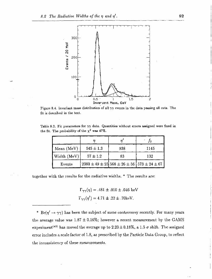
8.2 The Radiative Widths of the 77 and q’. 92
0.5 - 1 1.5 2 Invariant Mass, GeV
Figure 8.4. Invariant mass distribution of all 77 events in the data passing all cuts. The fit is described in the text.
Table 8.2. Fit parameters for 77 data. Quantities without errors assigned were fixed in the fit. The probability of the x2 was 47%.
1 Mean (MeV) 1 545 f 1.3 1 938 I 1145 I
1 Width (MeV) 1 57f 1.2 1 83 1 132 I
I Events I2380 f 49 f 251568 rt 26 f 56 1573 f 24 f 67 1
together with the results for the radiative widths. * The results are:
Py7(77) = .481 f .OlO f .046 keV
l?,,(q’) = 4.71 f .22 f .70keV.
* Br(q’ + 7-y) has been the subject of some controversy recently. For many years
the average value was 1.87 f 0.16%; h owever a recent measurement by the GAMS
experiment(43) has moved the average up to 2.23 f O.lS%, a 1.5 Q shift. The assigned
error includes a scale factor of 1.8, as prescribed by the Particle Data Group, to reflect
the inconsistency of these measurements.
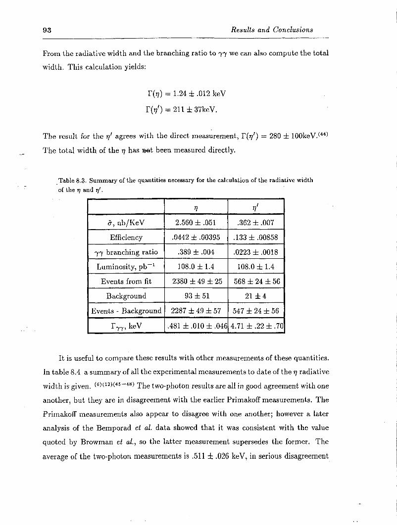
93 Results and Conclusions
From the radiative width and the branching ratio to yy we can also compute the total
width. This calculation yields:
I’(q) = 1.24 f .012 keV
I’(q’) = 211 f 3i’keV.
The result for the 7’ agrees with the direct measurement, I’(#) = 280 f 100keV.(44)
The total width of the q has r& been measured directly.
Table 8.3. Summary of the quantities necessary for the calculation of the radiative width of the q and r]‘.
6, nb/KeV
rl 77’ 2.560 f .051 .362 f .007
I~~ Efficiency 1 .0442 zt .00395 1 .133 f .00858 1
I yr branching ratio I .389 f .004 1 .0223 f .0018 1
v -’ Lumrnoslty, pb-l [ 108.0 f 1.4 ( iii.0 L1.4 1
I Events from fit 1 2380 f 49 f 25 1 568 f 24 f 56 1
I Background I 93 f 51 I 21 f4 I I Events - Background 1 2287 f49f57 ) 547f 24 f56 1
rrTi, keV 1 .481 f .OlO f .04614.71 f .22 f .701
It is useful to compare these results with other measurements of these quantities.
In table 8.4 a summary of all the experimental measurements to date of the 7 radiative
width is given. (6)(12)(45--48) Th e wo-photon results are all in good agreement with one t
another, but they are in disagreement with the earlier Primakoff measurements. The
Primakoff measurements also appear to disagree with one another; however a later
analysis of the Bemporad et al. data showed that it was consistent with the value
quoted by Browman et al., so the latter measurement supersedes the former. The
average of the two-photon measurements is .511 f .026 keV, in serious disagreement
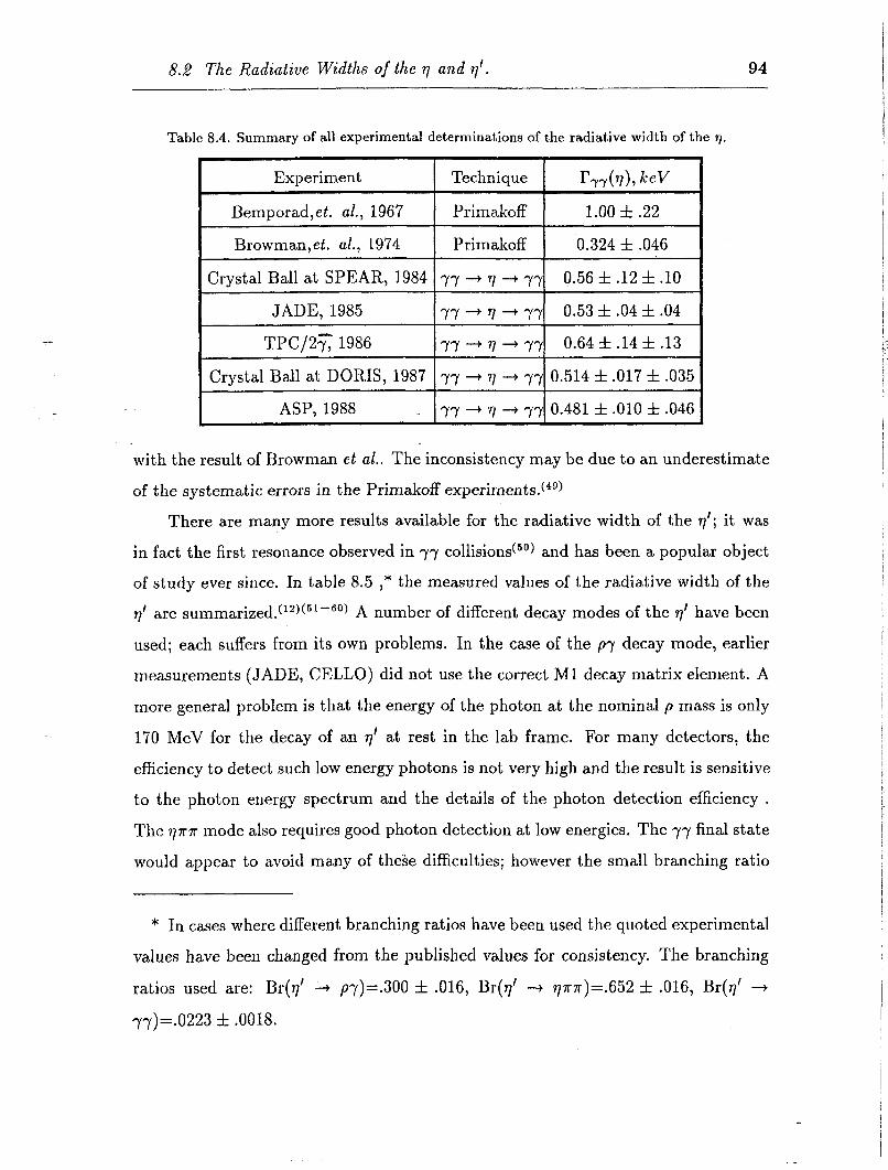
8.2 The Radiative Widths of the 77 and 7’. 94
Table 8.4. Summary of all experimental determinations of the radiative width of the 17.
-
ASP, 1988 77 + 77 -+ yy 0.481 f .OlO f .046
with the result of Browman et al.. The inconsistency may be due to an underestimate
of the systematic errors in the Primakoff experiments.(4g)
There are many more results available for the radiative width of the q’; it was
in fact the first resonance observed in yy collisions(50) and has been a popular object
of study ever since. In table 8.5 ,* the measured values of the radiative width of the
7’ are summarized.(‘2)(51-60) A number of different decay modes of the 7’ have been
used; each suffers from its own problems. In the case of the p-y decay mode, earlier
measurements (JADE, CELLO) d d i not use the correct Ml decay matrix element. A
more general problem is that the energy of the photon at the nominal p mass is only
170 MeV for the decay of an 7’ at rest in the lab frame. For many detectors, the
efficiency to detect such low energy photons is not very high and the result is sensitive
to the photon energy spectrum and the details of the photon detection efficiency .
The 777~ mode also requires good photon detection at low energies. The yy final state
would appear to avoid many of these difficulties; however the small branching ratio
* In cases where different branching ratios have been used the quoted experimental
values have been changed from the published values for consistency. The branching
ratios used are: Br(v’ -+ py)=.300 f .016, Br(q’ --+ ~7~)=.652 f .016, Br($ +
yy)=.O223 f .0018.
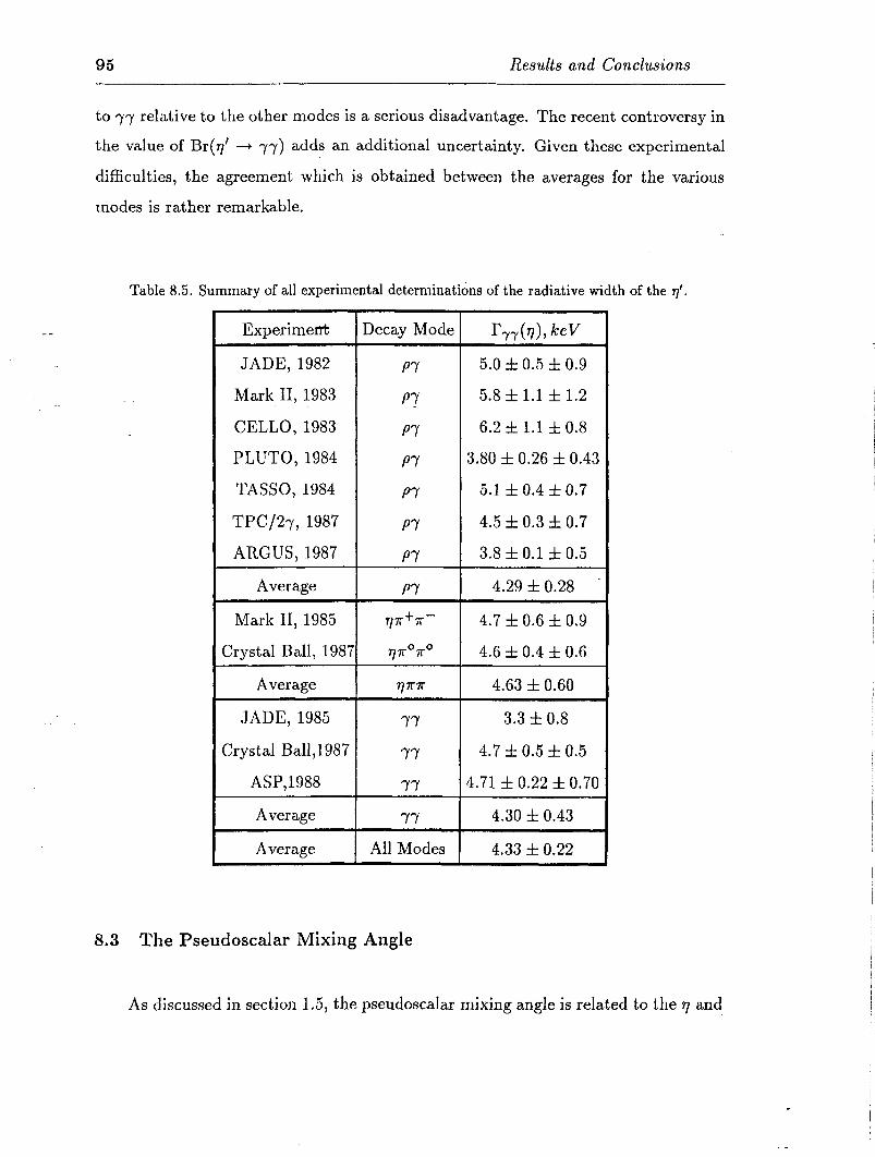
95 Results and Conclusions -
to yy relative to the other modes is a serious disadvantage. The recent controversy in
the value of Br(q’ + y-y) adds an additional uncertainty. Given these experimental
difficulties, the agreement which is obtained between the averages for the various
modes is rather remarkable.
Table 8.5. Summary of all experimental determinatidns of the radiative width of the r]‘.
Experimeti Decay Mode JJ,,h>, hV
JADE, 1982 PY 5.0 f 0.5 f 0.9
Mark II, 1983 P? 5.8 f 1.1 f 1.2
CELLO, 1983 PY 6.2 f 1.1 f 0.8
PLUTO, 1984 PY 3.80 f 0.26 f 0.43
TASSO, 1984 PY 5.1 f 0.4 f 0.7
TPC/2-y, 1987 PY 4.5 f 0.3 f 0.7
ARGUS, 1987 PY 3.8 f 0.1 f 0.5
Average PY 4.29 f 0.28 -
Mark II, 1985 ?pr+a- 4.7 f 0.6 f 0.9
Crystal Ball, 1987 qlr”n-o 4.6 f 0.4 f 0.6
Average VT 4.63 f 0.60
JADE, 1985 YY 3.3 f 0.8
Crystal Ball,1987 YY 4.7 f 0.5 f 0.5
ASP,1988 YY 4.71 f 0.22 f 0.70
Average YY 4.30 f 0.43
Average All Modes 4.33 f 0.22
8.3 The Pseudoscalar Mixing Angle
As discussed in section 1.5, the pseudoscalar mixing angle is related to the 7 and

8.3 The Pseudoscalar Mixing Angle 96
7’ radiative widths by:
rll-, = CL2 M3, -“rl sin t9 + J8 cos t9 I2
64~3 3 fa * fl * *
-
This is two equations in three unknowns: 8,, the pseudoscalar mixing angle, fs and
fi, the decay constants for the SU(3) basis states Q and ql . The latter cannot be
directly measured, so w:must make some assumptions. The usual one is that of oct,et
symmetry, in which fs = f?r because they belong in the same SU(3) octet. However,
- symmetry breaking effects turn out -to be rather large in this case; a calculation by
Donoghue, Holstein and Lin incorporating these corrections c61) yielded the result:
fi, = 1.25&r (8.1).
A similar calculation by Gasser and Leutwyler(62) gave a consistent result, fa = 1.21 f*. (Gilman and Kauffman(63) estimate the uncertainty on these calculations to
be on the order of 5%.) Using eq. 8.1 to define fs in terms of the measured value for
the pion decay constant, fX = 93 MeV, the radiative widths of the v and the q’ as
measured in this experiment give the following results:
. op = -19.8’ f 2.5’ (8.2)
fi = 1.04 f .llfr = 96 f 1lMeV
(Because the equations are quadratic in 6*, there are two possible solutions; the
ambiguity is resolved by independent measurements of 6,, for example in J/d decays.)
The errors include the 5% uncertainty on fi. Using this value of the pseudoscalar mixing angle in equation 1.25 gives the quark
content of the 77 and r,~’ mesons:
17) = .58juu + dd) - .57Jss)
17’) = .4Ojuii + dd) + .82(ss) w

8.3 The Pseudoscalar Mixing Angle ,
97
I
-
According to this result, both the 11 and 7’ have significant admixtures of 6; this is
not apparent in their decays, as they are both too light to decay into kaons. This
situation is far from the case of ‘ideal’ mixing, as exemplified by the Jpc = l--
nonet in which the mixing angle is approximately 35’ resulting in a p which is mostly
uu + dd, and decays primarily to pions, while the r.$ is mostly ss and decays primarily
to kaons. The tensor nonet is also very close to ideally mixed. The pseudoscalar nonet
may be so far from ideally mixed because the process dd H gluons H s;i; requires only
two gluons, as opposed?0 three for the vector nonet, and cys is larger due to the
lighter masses involved.(‘j4)
If we try to determine whether other states are also mixing with the q or q’, we
immediately run into the following problem: the addition of another state requires
a new mixing angle, and we must then attempt to solve 2 equations in 4 unknowns.
Even assuming a relationship between fs and fn, as we did above, this leaves us with
one extra variable. Because of the lack of knowledge concerning the value of fi it is
not possible to determine whether other states, such as charmonium or gluonium, are
mixing with the 7 or the 7’ from a measurement of the radiative widths alone.
There are other experiments which are sensitive to the pseudoscalar mix.ing angle,
such as measurements of J/$ decays and of radiative decays of the light vector mesons,
The results are compatible with measurements of the radiative widths, and so far there
is no evidence for mixing with additional states. (65~66) There is also agreement with
the theoretical prediction using the quadratic Gell-Mann Okubo mass formula:
4M& = Mi + 3( Mi cos2 Op + MG, sin2 19*), (8.4)
if one-loop chiral corrections are taken into account. c61)In a comprehensive review of
the subject, Gilman and Kauffman concluded that both theoretical predictions and
current experimental evidence are consistent with ep -N -2OO. in the framework of
the simple SU(3) mode1.(63).
--
8.4 Summary and Conclusions 98
8.4 Summary and Conclusions
Two-photon production of the 11 and $ mesons has been observed with the ASP
detector at the PEP e+e- storage ring. Both were detected in the +yy decay mode, in
an untagged configuration. The radiative widths of the 77 and 7’ were determined to
be:
bh) = .481 f -010 f .046 keV
ITrr(q’) = 4.71 f .22 f .70keV,
in agreement with previous measurements. (One exception to this is that the radiative
width of 77 as determined by the Primakoff technique is not in agreement with the
value found here.) The statistical accuracy of the measurements exceeds that of
any previous two-photon measurements using the yy decay mode, and the combined
statistical and systematic errors are comparable to the precision achieved in the most
accurate measurements to date. Using the measured radiative widths of the 77 and
q’, the pseudoscalar mixing angle is calculated. The result, 19~ = -19.8 f 2.5’, is in
agreement with other experimental methods which have been employed.
Appendix A
Forward Drift Chambers
- -
- In order to identify charged particles and measure their trajectory in the forward
direction, a system of forward drift chambers was designed and built as part of the
ASP detector. The forward drift chambers were located symmetrically on either
side of the interaction point between the inner and outer forward shower counters.
There were two drift chamber modules on each side, at z = f1.6 m, the ‘inner’ drift
chambers, and at z = f3.0 m, the ‘outer’ drift chambers. Each module consisted
of two drift chamber planes, one with the wires oriented vertically to measure the 2
coordinate and the other with wires oriented horizontally to measure the @ coordinate.
The angular acceptance of the outer drift chambers was 20 to 100 mr from the
beamline; for the inner drift chambers the acceptance was 50 to 190 mr. For charged
tracks which were from 50 to 100 mr the drift chambers provided two measurements
in li and 5 of the track. The forward drift chambers were the only components of
the ASP detector which were surveyed, providing a known frame of reference for the
geometry of the other detector elements.
In the following sections, the mechanical construction, electronic read-out and gas
system of the forward drift chambers will be described, followed by a brief discussion
of the performance.
A. 1 hIechanical Construction 100
A. 1 Mechanical Construction
As mentioned above, each of the four drift chamber modules consisted of two wire
planes, oriented orthogonally. Each of the eight drift chamber planes was constructed
from two halves which were rectangular in shape with a semi-circular cutout. Two of
these chambers were mounted on either side of the beampipe to create a square drift
chamber plane with a circular cutout to accomodate the beampipe. The radius of the
cutout was 3.15 in for the inner drift chamber modules and 2.15 in for the outer drift
chamber modules. Apartirom the difference in the size of the semi-circular cutout,
the sixteen individual chambers were identical in construction.
Each chamber had a machined aluminum skeleton consisting of a spine 39.6 in
long, and two L-shaped end-pieces 11.89 in wide which were joined to the spine with
dowels. The aluminum pieces were all .5 in thick and 1.77 in across. Holes for the
feed-throughs were drilled in the L-shaped end-pieces, so that the wires could be
strung parallel to the spine. There were two rows of 19 holes on .59 in spacing, for
a total of 38 wires in each chamber. The active area of the each chambers was 25.5
by 11.5 in, minus the semi-circular cutout. The read-out electronics were mounted
on both ends in the space formed by the L and the spine; slots in the aluminum were
machined so that the circuit boards could be slid in and out.
The chambers were covered on both sides with .063 in thick copper-clad G-10.
The G-10 was fastened to the aluminum skeleton with a row of screws on 1 in spacing.
An O-ring groove was machined in the aluminum spine and end-pieces inside the row
of screws to make the chambers gas tight. In addition, RTV was used on all joints.
A center ring of machined G-10 was glued inside the semi-circular cutout in the G-10
plate. The semi-circular ring consisted of three layers, each with slots machined in
them to allow the wires to be strung through them. After the wires were strung,
Dolph’s epoxy was injected into the slots to hold the wires. After it had cured the
wires were trimmed out of the semi-circle. The openings on either side of the G-10
ring were closed up by soldering thin copper skins to the G-10 plates and sealing the
edges with RTV.
The feedthroughs were machined from Delran and were a snug fit in the machined
,.. Q ;
: .,
.
101 Forward Drift Chambers
holes. To ensure that the chambers would be gas tight the feedthroughs were epoxied
in place. The wires which were strung through the feedthroughs were alternating
sense wires, of 30 pm gold-plated tungsten, and field wires, of 150 pm copper-plated
beryllium. The two rows of wires were arranged in an alternating pattern so that the
nearest neighbors of each sense wire were field wires. The tension in the wires was
set by weighting them with weights strung over a pulley. This tension was chosen
to ensure that the wire displacement due to gravitational sag would be insignificant.
The displacement, S, of a wirmf length 1 and weight per length w, strung at a tension
T, is given by WP
6=-. - BT
Fo,r the sense wires, a tension of 100 gm ensured that the gravitational sag would be
less than half the wire diameter. For the heavier field wires a tension of 300 gm was
required.
After the wires were strung they were held in place by inserting a pin into the
feedthrough with a drop of epoxy. The pin made electrical contact with the wire,
and it had an attached piece of multi-strand electrical wire which was soldered to a
circuit board for the electronic read-out. In the case of the field wires, this read-out
wire was soldered to a copper ground plate attached to the chamber body.
A.2 Operation and Electronic Read-Out
The chambers were operated at atmospheric pressure with a gas mixture of 48.2%
Argon, 4S.2% ethane and 1.6% ethyl alcohol vapor (C,H,O*). The alcohol vapor was
introduced by bubbling the gas through a container of ethyl alcohol (200 proof) at
0’ C. The purpose of the alcohol was to reduce the possibility of wire damage due
to the occasional high currents drawn by the chambers, which were located close to
the beampipe. Alcohol attacks epoxies which are not fully cured and may also attack
RTV if present in quantities greater than a few percent. However no damage due to
the alcohol was observed in the forward drift chambers.
The sense wires were operated at +2.6 kV and the field wires were at ground.
The signals from the sense wires were capacitively coupled to a Lecroy HIL440 hybrid
-
A.3 Performance 102
amplifier/discriminator, which came in a four-channel 24-pin dual in-line package.
This hybrid model had an externally adjustable threshold via a control voltage, and
required f5V and -2.5 V supplies. The output was a differential ECL twisted pair
cable, which carried the signal a couple hundred feet away to the electronics building.
There the signals were fed into time-to-amplitude modules (TAC’s), which produced
a signal proportional to the delay between the beam crossing and the observed signal.
This information was recorded on magnetic tape.
Each sense wire wasread out on one end only. Sense wires which intersected the
circular cut-out were of course read out on each end. For the large radius chambers
there were 5 such bisected wires, and there were 3 for the small-radius chambers.
Given 19 sense wires in each chamber, the total number of channels to read out was
24 and 22, respectively, for the large and small-radius chambers. The channel count
for all sixteen chambers was 368.
A circuit board was designed with four Lecroy hybrids, providing 16 channels
of read-out. However, on half of them only two hybrids were actually mounted; one
fully stuffed card and one half-stuffed card were then mounted on each end of the
chambers. In order to make it easy to replace a circuit board with dead channels,
the cards were designed to slide into Camac-style receptacles which were mounted on
another board to which the sense wire leads were soldered.
A.3 Performance
The drift chambers performed well; there were almost no dead channels and the
effects of beam-related noise were negligible due to copper shielding around the elec-
tronics and proper signal grounding. The occupancy was higher than expected from
single charged tracks on low-angle -Bhabha events, however, due to early showering
in the beam-pipe material. The extra hits made it difficult to determine the precise
trajectory for such tracks.
For charged tracks which did not begin to shower in the beam-pipe, signals would
be registered by two sense wires in each plane through which the track passed. The
time of the hit on each wire was proportional to the distance of the track from the
-
103 Forward Drift Chambers
wire; by comparing the measurements of the two wires, the error of the measurement
can be determined. This is shown in fig. A.l; the difference between the positions as
measured by two adjacent wires is plotted. The resolution is given by K* the result 6
is a resolution of about 300 pm.
I I I
0 Wre 1 - Wre 2, cm
Figure A.l. Difference between measured position of track from two adjacent wires in the drift chambers. The resolution for a single measurement is estimated from this to be about 300 pm.
The resolution was somewhat worse than expected; this was due to the fact the
drift velocity of ionized electrons was not constant over the width of a cell. Before the
alcohol vapor was added, the drift velocity had been roughly constant; however the
effect of alcohol is to raise the electric field strength at which the drift velocity reaches
a plateau. The calculated drift velocity across the cell both with and without alcohol
is shown in fig. A.2; the calculation used electrostatic field calculations performed on
a computer together with drift velocity vs. electric field measurements performed in
studies for the Mark11 vertex chamber.(‘j7)
A correction for this effect was applied but it was only an approximation, re-
sulting in a somewhat worsened resolution. However due to the long lever arm of
the forward drift chambers, the achieved resolution was satisfactory for studies of the
beamspot position and determination of geometry constants.

104
v)
3 6-
5 Q x - Ill- . lUgXXXx
t x x x x x x x
-0 Q G
Q
s 0 0
: 4- 0
c 0 0
Q Q Q ;f
0
2-
--
IIII III, III, I,,, ,,,I ,141 ‘0 25 5 75 10 . . 12.5 15
Distance From Sense Wire, mm
Figure A.2. Calculated drift velocity in forward drift chambers vs distance from sense wire. The X’s are for a gas mixture of 50% argon, 50% ethane. The O's are the same with the addition of 1.6% ethyl alcohol vapor.
References
1. Landau and Lifshitz, Phys. Zs. Soviet Union 6 (1934) 244
2. J. D. Jackson, Classical Electrodynamics, John Wiley and Sons, New York. 1962 p. 10.
3. Euler and Kockel, Naturwissenschaften26 (1935) 246
4. Breit and Wheeler, Phys. Rev. 46 (1934) 1087
5. H. Primakoff, Phys. Rev. 81 (1951) 899
6. C. Bemporad, et al., Phys. Lett. B25 (1967) 280
7. F. E. Low, Phys. Rev. 120 (1960) 582
105
8. E. Williams, Phys. Rev. 45 (1934 ) 729
9. C. F. von Weizszcker, Jzp88 (1934) 612
10. V. Balakin, et al., Phys. Lett. B34 (1971) 663
11. C. Bacci, et al., Nuovo Cim. 3 (1972) 709
12. D. Williams, et al.(Crystal Ball collaboration), Phys. Rev. D38 (1988) 1365
13. For a summary of the Feynman rules, see J. Bjorken and S. Drell, Relativisitic Quantum Mechanics McGraw Hill, New York, 1964. .
14. V. Budnev, et al., Phys. Rep. 15 (1975) lS1
15. J. Bjorken and S. Drell, Relativisitic Quantum Mechanics, McGraw Hill, New York, 1964.
16. M. Poppe, Int. J. Mod. Phys. 1 (1986) 545
17. C. N. Yang, Jpr77 (1950) 242
18. S. Adler, Phys. Rev. 177 (1969) 2426 J.S. Bell and L. Jakiw, Nuovo Cim. 60 (1969) 47
19. D. L. Burke, R. Hollebeek, et al.“Proposal to Search for Weakly-Interacting Particles using Photon Tagging”, PEP Proposal 021, March 1983.
20. E. Ma and J. Okada, Phys. Rev. D18 (1978) 4219
21. G. Barbiellini, B. Richter, J. Siegrist, Phys. Lett. B106 (1981) 414
22. C. Hearty, et al., Phys. Rev. Lett. 58 (1987) 1711
23. P. Grannis, D. Jaffe and M. Marx, Nucl. Instr. and Meth. 188 (1981) 239
24. P. Levy, et al., Jour. Am. Ceram. SOS. 57 (1974) 176
25. The pulser used was similar to that described by L. R. Fortney in Proceedings of the Calorimeter Calibration Worlcshop,edited by H. Jostlein (Fermi National AcceleratorLaboratory, Batavia, Illinois, 1983), p. 1.
26. J. Menefee and Y. Cho, IEEE Trans. Nucl. Sci. NS-12 (1966) 159

106
27. J. S. Beale, et al., Nucl. Instr. and Meth. 117 (1974) 501
28. E. Cisnero, et al., IEEE Trans. Nucl. Sci. NS-28 (1981) 465 M. Breidenbach et al., IEEE Trans. Nucl. Sci. NS-25 (1978) 706
29. For details of the ASP trigger system, see: R. J. Wilson, Proceedings of the Workshop on Triggering, Data Acquisition and Computing for High En- ergy/High Luminosity Ha&on-Ha&on Colliders, edited by B. Cox, R. Fenner, and P. Hale (Fermi National Accelerator Laboratory, Batavia, Illinois, 1986), p. 118.
-- 30. R. L. Ford, W. R-elson, “The.EGS Code System: Computer Programs for the Monte Carlo Simulation of Electromagnetic Cascade Showers (Version 3)“, SLAC-PUB-0210, June 1978.
31. O.Dahl, et al., Lawrence Berkeley Laboratory, Group A Programming Note # P-126, July 1968.
32. J. Vermaseren, Nucl. Phys. B229 (1983) 347
33. S. Brodsky and P. Lepage, Phys. Rev. D24 (1981) 1808
34. D. Karlen, Nucl. Phys. B289 (1987) 23
35. I-1. Cheng,E.Tsai,X.Zhu, Phys. Rev. D26 (1982) 922
36. Tony Barker and Willy Langeveld, private communication.
37. R.L. Walker, in Proceedings of the 4th International Symposium on Electron and Photon Interactions, p 36 (1969).
38. S.J. deJong, J.A.M. Vermaseren, AX0 User Manual, NIKHEF-H, March 1988 (unpublished).
39. F.A. Berends, P.H. Daverveldt, and R. Kleiss, Comp. Phys. Comm. 40 (1986) 309
40. Christopher A. Hawkins, private communication.
41. For a more detailed description of the luminosity analysis, see Christopher A. Hawkins, thesis, Stanford University, 1988 (unpublished).
42. F. James and M. ROOS, Comp. Phys. Comm. 10 (1975) 343

107
43. D. Alde, et al., Z. Phys. C36 (1987) 603
44. D. Binnie, et al., Phys. Lett. B83 (1979) 141
45. A. Browman, et al., Phys. Rev. Lett. 32 (1974) 1067
46. A. Weinstein, et aZ.(Crystal Ball collaboration), Phys. Rev. D28 (1983) 2896
47. W. Bartel, et aZ.(JADE collaboration), Phys. Lett. B160 (1985) 421
-- 48. II. Aihara, et uZ.(TPC/2y collaboration), Phys. Rev. D33 (1986) 844
-
49. N. Roe, Mini-review of I’,,(v), in the 1987 Review of Particle Properties, to be published.
50. G. Abrams, et aZ.(MarkII collaboration), Phys. Rev. Lett. 43 (1979) 477
51. P. Jenni, et uZ.(MarkII collaboration), Phys. Rev. D27 (1983) 1031
52. W. Bartel, et aZ.(JADE collaboration), Phys. Lett. B113 (1982) 190
53. 13. Berend, et aZ.(CELLO collaboration), Phys. Lett. B114 (1982) 378
54. C. Berger, et aZ.(PLUTO collaboration), Phys. Lett. B142 (1984) 125
55. M. Althof, et uZ.(TASSO 11 b co a oration), Phys. Lett. B147 (1984) 487
56. I-1. Aihara, et aZ.(TPC/2y collaboration), Phys. Rev. D35 (1987) 2650
57. I-I. Albrecht, et aZ.(ARGUS collaboration), Phys. Lett. B199 (1987) 457
58. G. Gidal, et aZ.(MarkII collaboration), Phys. Rev. Lett. 59 (1987) 2012
59. D. Antreasyan, et aZ.(Crystal Ball collaboration), Phys. Rev. D36 (1987) 2633
60. W. Bartel, et aZ.(JADE collaboration), Phys. Lett. Bl6O (1985) 421
61. J. Donoghue,B. Holstein and Y. Lin, Phys. Rev. Lett. 55 (1985) 2766
62. J. Gasser and I-I. Leutwyler, Nucl. Phys. B250 (1985) 465
63. F. Gilman and R. Kauffman, Phys. Rev. D36 (1987) 2761
64. A. De Rtijula, H. Georgi, and S. Glashow, Phys. Rev. D12 (1975) 147

108
65. J. Rosner, in Proceedings of the 1985 International Symposium on Lepton and Photon Interactions at High Energies, Kyoto, Japan 1985, edited by M. Kon- uma and K. Takahashi, p. 448.
66. A. Seiden, E-1. Sadrozinski and H. Haber, SCIPP 87/X3 (unpublished).
67. Rene Ong, private communication.