Slab stress and strain rate as constraints on global mantle flow

Laura Alisic,1 Michael Gurnis,1 Georg Stadler,2 Carsten Burstedde,2 Lucas C. Wilcox,3

and Omar Ghattas2,4,5

Received 28 August 2010; revised 8 October 2010; accepted 14 October 2010; published 23 November 2010.

[1] Dynamically consistent global models of mantleconvection with plates are developed that are consistentwith detailed constraints on the state of stress and strainrate from deep focus earthquakes. Models that best fitplateness criteria and plate motion data have strong slabsthat have high stresses. The regions containing the MW 8.3Bolivia and MW 7.6 Tonga 1994 events are considered indetail. Modeled stress orientations match stress patternsfrom earthquake focal mechanisms. A yield stress of atleast 100 MPa is required to fit plate motions and matchesthe minimum stress requirement obtained from the stressdrop for the Bolivia 1994 deep focus event. The minimumstrain rate determined from seismic moment release in theTonga slab provides an upper limit of ∼200 MPa on thestrength in the slab. Citation: Alisic, L., M. Gurnis, G. Stadler,C. Burstedde, L. C. Wilcox, and O. Ghattas (2010), Slab stress andstrain rate as constraints on global mantle flow, Geophys. Res.Lett., 37, L22308, doi:10.1029/2010GL045312.

1. Introduction

[2] An essential component of mantle convection modelswith plates is the strength of the subducting slabs and theirinfluence on the dynamics of the convective system. Thestronger slabs are, the more they could exert an importantforce on plate motions, acting as stress guides. Regionalstudies using the geoid concluded that the viscosity in theslabs is 100 to 1000 times higher than in the surroundingmantle [Moresi and Gurnis, 1996], and could not exceed1023 Pa s in order to fit geoid highs over subducted slabs[Billen et al., 2003]. Also, studies of plate bending indicatethat the plate viscosity must be between 50 and 200 timesthe mantle viscosity in order to fit dissipation constraints[Conrad and Hager, 1999]. Torque balance models of thePacific and Australian plate suggested that the best fit toobserved rotation poles was obtained with an effectivelithosphere viscosity of 6 × 1022 Pa s [Buffett and Rowley,2006]. In contrast, with time‐dependent generic models ofslab dynamics, strong slabs are inferred [Billen and Hirth,2007], in concordance with experimentally found tempera-ture dependence of the effective viscosity of olivine [Hirth

and Kohlstedt, 2003]. Using a composite rheology with anonlinear component [Billen and Hirth, 2007] allows forlocalization of strain, and hence localized strain weakeningin the hinge of a subducting slab. In this way, slabs can bestrong and still subduct with relative ease. Global modelsaddressing slab pull show that strong slabs provide the bestfit to observed plate motions, exerting slab pull forces thataccount for approximately half of the total driving forces onplates [Conrad and Lithgow‐Bertelloni, 2002].[3] The state of stress indicated by earthquake focal

mechanisms and their stress drop, in selected cases, provideadditional constraints on the strength of slabs. The stressdrop estimates for large moment magnitude deep earth-quakes form a lower limit of the stress that the slab mustsustain. Here the state of stress of slabs is studied in globallyconsistent dynamic models of mantle convection with plates,while incorporating a composite rheology. We address twostudy areas, covering the locations of the Bolivia, MW 8.3,1994 and the Tonga, MW 7.6, 1994 earthquakes. Theseearthquakes were chosen because they putatively representend member types of deep earthquakes. The Bolivia earth-quake experienced a large stress drop of 114 MPa, a rupturepropagation of only 1 km/s, few aftershocks, and waslocated in a region with scarce seismicity [Kanamori et al.,1998]. In contrast, the Tonga earthquake had a low stressdrop (∼1.6 MPa), fast rupture propagation of 3–4 km/s, andmany aftershocks in a region with abundant seismicity[Wiens and McGuire, 1995].

2. Model Setup and Solution

[4] The dynamics of instantaneous mantle convection aregoverned by the equations of conservation of mass andmomentum. Under the Boussinesq approximation for amantle with uniform composition and the assumption thatthe mantle deforms viscously, the nondimensionalized formof these equations is [e.g., Schubert et al., 2001]:

#� u ¼ 0; ð1Þ

#

p� #� � T ; uð Þ #

uþ #

u>� �� � ¼ Ra T er; ð2Þ

where u, p, h, and T are the velocity, pressure, viscosity, andtemperature, respectively; and er is the unit vector in theradial direction. Ra is the Rayleigh number, Ra =ar0gDTD3/(�h0), where a, r0, h0, and � are the referencecoefficients of thermal expansion, density, viscosity, andthermal diffusivity (see Table 1 in the supplementarymaterial of Stadler et al. [2010]). DT is the temperaturedifference across a mantle with thickness D, and g is thegravitational acceleration.[5] We solve these equations with finite elements using a

code (Rhea) that exploits Adaptive Mesh Refinement (AMR)

1Seismological Laboratory, California Institute of Technology,Pasadena, California, USA.

2Institute for Computational Engineering and Sciences, Universityof Texas at Austin, Austin, Texas, USA.

3HyPerComp, Westlake Village, California, USA.4Jackson School of Geosciences, University of Texas at Austin, Austin,

Texas, USA.5Department of Mechanical Engineering, University of Texas at

Austin, Austin, Texas, USA.

Copyright 2010 by the American Geophysical Union.0094‐8276/10/2010GL045312

GEOPHYSICAL RESEARCH LETTERS, VOL. 37, L22308, doi:10.1029/2010GL045312, 2010

L22308 1 of 5

[Burstedde et al., 2008]. Rhea is a new generation mantleconvection code, using forest‐of‐octree‐based adaptivemeshes. With Rhea’s adaptive capabilities we create localresolution down to ∼1 km around plate boundaries, whilekeeping the mesh at a much coarser resolution away fromsmall features. The global models in this study haveapproximately 200 million elements, a reduction of a factor∼5000 compared to a uniform mesh of the same high reso-lution [Stadler et al., 2010].[6] A composite formulation of Newtonian (diffusion

creep) and non‐Newtonian (dislocation creep) rheology isimplemented along with yielding. Plate boundaries aremodeled as narrow weak zones with a defined viscosityreduction of several orders of magnitude. A generalizedviscosity law for the Earth’s mantle is used:

� ¼ G xð Þ dp

A COHr

� �1n

_�1�nnII exp

Ea þ PVa

nRT

� �; ð3Þ

where h is viscosity in Pa s, d grain size in mm, COH watercontent in parts per million of silicon, n is the stress exponent,and _�II the second invariant of the strain rate tensor in s−1.Ea is the activation energy in J/mol, P lithostatic pressurein Pa, Va activation volume in m3/mol, R the gas constant,

and T the temperature in K. G(x) is a reduction factor used todefine weak zones, and is set to between 1 × 10−5 and 5 × 10−3

in plate boundaries and to 1 elsewhere. The parameters A, n, rand p are determined experimentally [Hirth and Kohlstedt,2003]. The composite viscosity [Billen and Hirth, 2007] isobtained by combining diffusion creep (hdf) and dislocationcreep (hds) using a harmonic mean. Then, a yield criterionwith yield strength sy is imposed to obtain an effectiveviscosity:

�comp ¼ �df �ds�df þ �ds

; ð4Þ

�eff ¼ min�y

_�II; �comp

� �: ð5Þ

The yielding law is only applied if the local temperature islower than the yield temperature Ty. See Table 2 in thesupplementary material of Stadler et al. [2010] for a sum-mary of the parameter values used in the presented models.[8] Since plate velocities and “plateness” are outcomes,

both the full buoyancy field and plate boundary details at afine scale must be incorporated. The global models areconstructed with oceanic plate ages [Müller et al., 2008], a

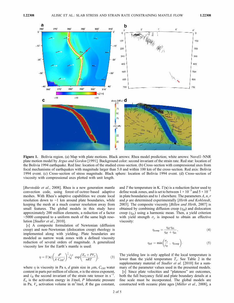
Figure 1. Bolivia region. (a) Map with plate motions. Black arrows: Rhea model prediction; white arrows: Nuvel1‐NNRplate motion model by Argus and Gordon [1991]. Background color: second invariant of the strain rate. Red star: location ofthe Bolivia 1994 earthquake. Red line: location of the studied cross‐section. (b) Cross‐section with compressional axes fromfocal mechanisms of earthquakes with magnitude larger than 5.0 and within 100 km of the cross‐section. Red axis: Bolivia1994 event. (c) Cross‐section of stress magnitude. Black sphere: location of Bolivia 1994 event. (d) Cross‐section ofviscosity with compressional axes plotted with unit length.

ALISIC ET AL.: SLAB STRESS AND STRAIN RATE CONSTRAINING MANTLE FLOW L22308L22308

2 of 5

thermal model containing slabs in the upper mantle, andtomography in the lower mantle [Ritsema et al., 2004].Current tomography resolves slabs in the upper mantlepoorly, as mantle wedges and slabs typically blur together.However, resolving the slabs as high‐viscosity stress guidesis critical for correctly predicting plate motions [e.g., Zhonget al., 1998]. In order to maximize the slab sharpness, theupper mantle structure was created with slab contours fromseismicity [Gudmundsson and Sambridge, 1998].

3. Results

[9] Computed models predict velocity, viscosity, strainrate, stress magnitude, orientation of the stress axes, andenergy dissipation. The models are tested by assessing theplateness of the surface velocity field, and its misfit withinferred surface velocities. The current best model has ayield stress of 100 MPa and stress exponent of 3.0 [Stadleret al., 2010], with deformation highly localized around plateboundaries. Plate interiors and slabs have a viscosity of∼1024 Pa s. The hinge of subducting plates yields, causingthe viscosity in the hinge to drop to ∼ 5 × 1022 to 1023 Pa s,consistent with estimates of Billen et al. [2003] andWu et al.[2008]. This global model allows us to study the local state

of stress in a globally consistent framework, includingBolivia and Tonga.[10] First, we consider the region containing the 1994 MW

8.3 Bolivia event (647 km depth), where Nazca subductsunder the South‐American plate at ∼8 cm/year [Bird, 2003].High strain rates are found exclusively in the trench, indi-cating highly localized deformation at the plate boundaries(Figure 1a). The Bolivia 1994 earthquake experienced aminimum frictional stress of 55 MPa and a static stress dropof 114 MPa [Kanamori et al., 1998]. This provides anestimate of the minimum stress needed in the slab. There areseveral other deep earthquakes with large predicted stressdrops in the same region, including the 1970 Colombia (MW

8.3) earthquake with a stress drop of 68 MPa [Fukao andKikuchi, 1987; Ruff, 1999]. The modeled slab allows forthese stress drops, and shows ambient stresses that arealmost everywhere equal to the yield stress, 100 MPa(Figure 1c). Locally, the stress is even greater, namelywhere the temperature is higher than the yield temperature.The modeled state of stress in the nominal model is in goodagreement with earthquake focal mechanisms (Figures 1band 1d). The stress axes indicate downdip tension in thehinge and shallow to intermediate depths in the slab, andcompression in the deeper parts. This transition from tension

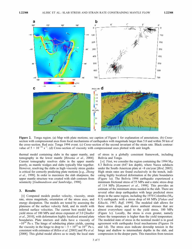
Figure 2. Tonga region. (a) Map with plate motions; see caption of Figure 1 for explanation of annotations. (b) Cross‐section with compressional axes from focal mechanisms of earthquakes with magnitude larger than 5.0 and within 50 km ofthe cross‐section. Red axis: Tonga 1994 event. (c) Cross‐section of the second invariant of the strain rate. Black contour:value of 5 × 10−16 s−1. (d) Cross‐section of viscosity with compressional axes plotted with unit length.

ALISIC ET AL.: SLAB STRESS AND STRAIN RATE CONSTRAINING MANTLE FLOW L22308L22308

3 of 5

to compression around 300 km depth is consistent with thefocal mechanisms of Isacks and Molnar [1971].[11] The second case study focuses on the northern Tonga

region, containing the 1994 MW 7.6 earthquake. This is ahighly complex area with several microplates and rapidtrench rollback [Bird, 2003] (Figure 2a). The strain rate againindicates that the deformation almost exclusively occurs at

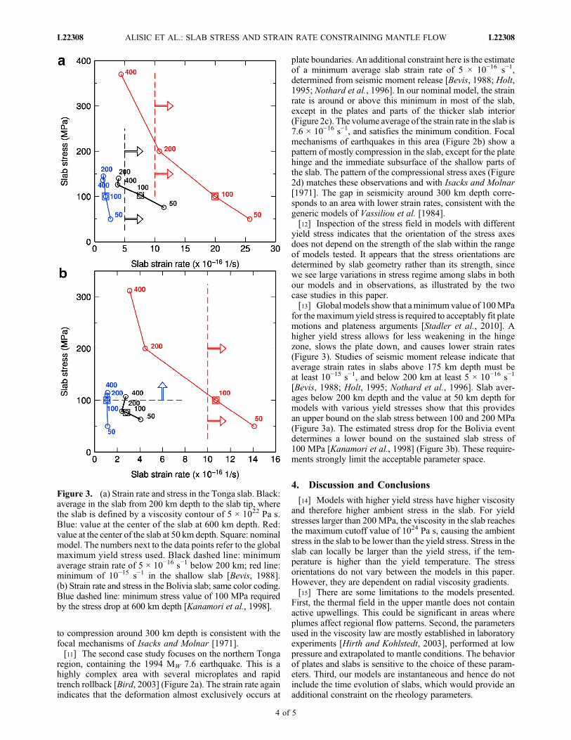
plate boundaries. An additional constraint here is the estimateof a minimum average slab strain rate of 5 × 10−16 s−1,determined from seismic moment release [Bevis, 1988; Holt,1995; Nothard et al., 1996]. In our nominal model, the strainrate is around or above this minimum in most of the slab,except in the plates and parts of the thicker slab interior(Figure 2c). The volume average of the strain rate in the slab is7.6 × 10−16 s−1, and satisfies the minimum condition. Focalmechanisms of earthquakes in this area (Figure 2b) show apattern of mostly compression in the slab, except for the platehinge and the immediate subsurface of the shallow parts ofthe slab. The pattern of the compressional stress axes (Figure2d) matches these observations and with Isacks and Molnar[1971]. The gap in seismicity around 300 km depth corre-sponds to an area with lower strain rates, consistent with thegeneric models of Vassiliou et al. [1984].[12] Inspection of the stress field in models with different

yield stress indicates that the orientation of the stress axesdoes not depend on the strength of the slab within the rangeof models tested. It appears that the stress orientations aredetermined by slab geometry rather than its strength, sincewe see large variations in stress regime among slabs in bothour models and in observations, as illustrated by the twocase studies in this paper.[13] Global models show that aminimum value of 100MPa

for themaximum yield stress is required to acceptably fit platemotions and plateness arguments [Stadler et al., 2010]. Ahigher yield stress allows for less weakening in the hingezone, slows the plate down, and causes lower strain rates(Figure 3). Studies of seismic moment release indicate thataverage strain rates in slabs above 175 km depth must beat least 10−15 s−1, and below 200 km at least 5 × 10−16 s−1

[Bevis, 1988; Holt, 1995; Nothard et al., 1996]. Slab aver-ages below 200 km depth and the value at 50 km depth formodels with various yield stresses show that this providesan upper bound on the slab stress between 100 and 200 MPa(Figure 3a). The estimated stress drop for the Bolivia eventdetermines a lower bound on the sustained slab stress of100 MPa [Kanamori et al., 1998] (Figure 3b). These require-ments strongly limit the acceptable parameter space.

4. Discussion and Conclusions

[14] Models with higher yield stress have higher viscosityand therefore higher ambient stress in the slab. For yieldstresses larger than 200 MPa, the viscosity in the slab reachesthe maximum cutoff value of 1024 Pa s, causing the ambientstress in the slab to be lower than the yield stress. Stress in theslab can locally be larger than the yield stress, if the tem-perature is higher than the yield temperature. The stressorientations do not vary between the models in this paper.However, they are dependent on radial viscosity gradients.[15] There are some limitations to the models presented.

First, the thermal field in the upper mantle does not containactive upwellings. This could be significant in areas whereplumes affect regional flow patterns. Second, the parametersused in the viscosity law are mostly established in laboratoryexperiments [Hirth and Kohlstedt, 2003], performed at lowpressure and extrapolated to mantle conditions. The behaviorof plates and slabs is sensitive to the choice of these param-eters. Third, our models are instantaneous and hence do notinclude the time evolution of slabs, which would provide anadditional constraint on the rheology parameters.

Figure 3. (a) Strain rate and stress in the Tonga slab. Black:average in the slab from 200 km depth to the slab tip, wherethe slab is defined by a viscosity contour of 5 × 1022 Pa s.Blue: value at the center of the slab at 600 km depth. Red:value at the center of the slab at 50 km depth. Square: nominalmodel. The numbers next to the data points refer to the globalmaximum yield stress used. Black dashed line: minimumaverage strain rate of 5 × 10−16 s−1 below 200 km; red line:minimum of 10−15 s−1 in the shallow slab [Bevis, 1988].(b) Strain rate and stress in the Bolivia slab; same color coding.Blue dashed line: minimum stress value of 100 MPa requiredby the stress drop at 600 km depth [Kanamori et al., 1998].

ALISIC ET AL.: SLAB STRESS AND STRAIN RATE CONSTRAINING MANTLE FLOW L22308L22308

4 of 5

[16] Stress drops of earthquakes provide a valuable con-straint on the minimum stress sustained in a plate or slab. Theactual stress drop on a fault can be highly heterogeneous dueto spatial variability of stress and strength on the fault plane.This could result in high local stress drop compared to theaverage over the fault [Venkataraman and Kanamori, 2004].Stress drops are determined from seismic moment and rupturearea, and accurately determining the rupture area remains anactive field of research [Venkataraman and Kanamori, 2004;Kanamori and Brodsky, 2004]. Also, there is currently nomethod available to determine how much higher the actualstress is compared to the stress drop [Kanamori and Brodsky,2004]. A recent study of exhumed ultramafic pseudotachy-lytes suggests that higher stresses could be required in slabsthan previously inferred from earthquake inversions; theestimated stress drop determined from the geologic record fordeep earthquakes in Corsica is at least 220 MPa, and could beas much as 580 MPa [Andersen et al., 2008].[17] In our models, the localization of strain in the hinges

of subducting slabs causes significant weakening of thematerial up to 2 orders of magnitude in viscosity. Thisprocess allows the rest of the slab to remain strong whilestill having sufficiently fast moving plates. Pointwise thedissipation of energy in the mantle is highest in the sub-ducting plate hinges, but the integration over this very smallvolume compared to the rest of the mantle results in only3%–5% of the total dissipation [Stadler et al., 2010]. This isconsistent with findings by Leng and Zhong [2010].[18] We have studied the state of stress in slabs in globally

consistent dynamic models of mantle convection with plates,and are able to reproduce the general trends in stress orien-tations in the Bolivia and Tonga case studies as observed fromearthquake focal mechanisms. These models have strongslabs and weak subducting plate hinges, such that the dissi-pation in the bending areas of plates is small compared to thetotal dissipation of energy from the mantle. A lower bound onthe strength of slabs is provided by the stress drop in strongdeep earthquakes. Because models with higher yield stresshave lower strain rates in slabs, the minimum average strainrate in slabs determined from seismic moment release givesan upper bound on the strength of the slabs.

[19] Acknowledgments. We thank H. Kanamori and D. Stegman forhelpful discussions. This work was partially supported by NSF’s PetaAppsprogram (OCI‐0749334, OCI‐0748898), NSF Earth Sciences (EAR‐0426271, EAR‐0810303), and the Caltech Tectonics Observatory (by theGordon and Betty Moore Foundation). Computing resources on TACC’sRanger and Spur systems were provided through the NSF TeraGrid undergrant number TG‐MCA04N026. The figures in this paper were producedusing GMT and Paraview.

ReferencesAndersen, T. B., K. Mair, H. Austrheim, Y. Y. Podladchikov, and J. C.Vrijmoed (2008), Stress release in exhumed intermediate and deep earth-quakes determined from ultramafic pseudotachylyte, Geology, 36(12),995–998.

Argus, D. F., and R. G. Gordon (1991), No‐net‐rotation model of currentplate velocities incorporating plate motion model NUVEL‐1, Geophys.Res. Lett., 18(11), 2039–2042.

Bevis, M. (1988), Seismic slip and down‐dip strain rates in Wadati‐Benioffzones, Science, 240(4857), 1317–1319.

Billen, M. I., and G. Hirth (2007), Rheologic controls on slab dynamics,Geochem. Geophys. Geosyst., 8, Q08012, doi:10.1029/2007GC001597.

Billen, M. I., M. Gurnis, and M. Simons (2003), Multiscale dynamics of theTonga‐Kermadec subduction zone, Geophys. J. Int., 153(2), 359–388.

Bird, P. (2003), An updated digital model of plate boundaries, Geochem.Geophys. Geosyst., 4(3), 1027, doi:10.1029/2001GC000252.

Buffett, B. A., and D. Rowley (2006), Plate bending at subduction zones:Consequences for the direction of plate motions, Earth Planet. Sci. Lett.,245(1–2), 359–364.

Burstedde, C., O. Ghattas,M. Gurnis, E. Tan, T. Tu, G. Stadler, L. C.Wilcox,and S. Zhong (2008), Scalable adaptive mantle convection simulation onpetascale supercomputers, in SC’08: Proceedings of the InternationalConference for High Performance Computing, Networking, Storage,and Analysis, pp. 1–15, IEEE Press, Piscataway, N. J.

Conrad, C. P., and B. H. Hager (1999), Effects of plate bending andfault strength at subduction zones on plate dynamics, J. Geophys.Res., 104(B8), 17,551–17,571.

Conrad, C. P., and C. Lithgow‐Bertelloni (2002), How mantle slabs driveplate tectonics, Science, 298(5591), 207–209.

Fukao, Y., and M. Kikuchi (1987), Source retrieval for mantle earthquakesby iterative deconvolution of long‐period P‐waves, Tectonophysics,144(1–3), 249–269.

Gudmundsson, Ó., and M. Sambridge (1998), A regionalized upper mantle(RUM) seismic model, J. Geophys. Res., 103(B4), 7121–7136.

Hirth, G., and D. Kohlstedt (2003), Rheology of the upper mantle and themantle wedge: A view from the experimentalists, in Inside the SubductionFactory, Geophys. Monogr. Ser., vol. 138, edited by J. Eiler, pp. 83–105,AGU, Washington, D. C.

Holt, W. E. (1995), Flow fields within the Tonga Slab determined from themoment tensors of deep earthquakes,Geophys. Res. Lett., 22(8), 989–992.

Isacks, B., and P. Molnar (1971), Distribution of stresses in the descendinglithosphere from a global survey of focal‐mechanism solutions of mantleearthquakes, Rev. Geophys., 9(1), 103–174.

Kanamori, H., and E. Brodsky (2004), The physics of earthquakes, Rep.Prog. Phys., 67, 1429–1496.

Kanamori, H., D. L. Anderson, and T. H. Heaton (1998), Frictional meltingduring the rupture of the 1994 Bolivian earthquake, Science, 279(5352),839–842.

Leng, W., and S. Zhong (2010), Constraints on viscous dissipation of platebending from compressible mantle convection, Earth Planet. Sci. Lett.,297, 154–164.

Moresi, L., and M. Gurnis (1996), Constraints on the lateral strength ofslabs from three‐dimensional dynamic flow models, Earth Planet. Sci.Lett., 138, 15–28.

Müller, R. D., M. Sdrolias, C. Gaina, and W. R. Roest (2008), Age, spread-ing rates, and spreading asymmetry of the world’s ocean crust, Geochem.Geophys. Geosyst., 9, Q04006, doi:10.1029/2007GC001743.

Nothard, S., J. Haines, and J. Jackson (1996), Distributed deformation inthe subducting lithosphere at Tonga, Geophys. J. Int., 127, 328–338.

Ritsema, J., H. J. van Heijst, and J. H. Woodhouse (2004), Global transitionzone tomography, J. Geophys. Res., 109, B02302, doi:10.1029/2003JB002610.

Ruff, L. J. (1999), Dynamic stress drop of recent earthquakes: Variationswithin subduction zones, Pure Appl. Geophys., 154, 409–431.

Schubert, G., D. L. Turcotte, and P. Olson (2001), Mantle Convection inthe Earth and Planets, Cambridge Univ. Press, Cambridge, U. K.

Stadler, G., M. Gurnis, C. Burstedde, L. C. Wilcox, L. Alisic, and O. Ghattas(2010), The dynamics of plate tectonics and mantle flow: From local toglobal scales, Science, 329, 1033–1038.

Vassiliou, M., B. Hager, and A. Raefsky (1984), The distribution of earth-quakes with depth and stress in subducting slabs, J. Geodyn., 1, 11–28.

Venkataraman, A., and H. Kanamori (2004), Observational constraints onthe fracture energy of subduction zone earthquakes, J. Geophys. Res.,109, B05302, doi:10.1029/2003JB002549.

Wiens, D. A., and J. J. McGuire (1995), The 1994 Bolivia and Tongaevents: Fundamentally different types of deep earthquakes?, Geophys.Res. Lett., 22(16), 2245–2248.

Wu, B., C. P. Conrad, A. Heuret, C. Lithgow‐Bertelloni, and S. Lallemand(2008), Reconciling strong slab pull and weak plate bending: The platemotion constraint on the strength of mantle slabs, Earth Planet. Sci. Lett.,272(1–2), 412–421.

Zhong, S., M. Gurnis, and L. Moresi (1998), Role of faults, nonlinear rhe-ology, and viscosity structure in generating plates from instantaneousmantle flow models, J. Geophys. Res., 103(B7), 15,255–15,268.

L. Alisic and M. Gurnis, Seismological Laboratory, California Instituteof Technology, Pasadena, CA 91125, USA. (alisic@gps.caltech.edu)C. Burstedde and O. Ghattas, Institute for Computational Engineering

and Sciences, University of Texas at Austin, Austin, TX 78712, USA.G. Stadler, Institute for Computational Engineering and Sciences,

University of Texas at Austin, Austin, TX 78712, USA.L. C. Wilcox, HyPerComp, 2629 Townsgate Rd. #105, Westlake Village,

CA 91361, USA.

ALISIC ET AL.: SLAB STRESS AND STRAIN RATE CONSTRAINING MANTLE FLOW L22308L22308

5 of 5