Skill-biased Technological Change, Earnings of Unskilled … · 2018-10-29 · 1 Skill-biased...

1

Skill-biased Technological Change, Earnings of Unskilled Workers, and Crime

Naci Mocan Louisiana State University, NBER and IZA

[email protected]

Bulent Unel Louisiana State University

[email protected]

September 2011

PRELIMINARY DRAFT

ABSTRACT

This paper investigates the impact of unskilled workers’ wages on crime. Following the literature on wage inequality and skill-biased technological change, we employ CPS data from 1980 to 2005 and create a state-and-year specific measure of skill-biased technological change, which is then used as an instrument for unskilled workers’ earnings in crime regressions. Regressions that employ state panels reveal that technology-induced variations in unskilled workers’ earnings impact property crime with an elasticity of -1.0. We find that earnings of non-college educated males impact crime, but that earnings of unskilled females have no influence on criminal activity. Estimating a structural crime equation using micro data from NLSY97 and instrumenting real wages of young workers with industry-year-state specific technology shocks, yields elasticities that are in the neighborhood of -1.7 for most types of crime. In both data sets there is evidence for asymmetric impact of unskilled workers earnings on crime. A decline in earnings has a larger effect on crime in comparison to an increase in earnings by the same absolute value.

We thank Deokrye Baek, Elif Filiz and especially Duha Altindag for outstanding research assistance.

2

Skill-biased Technological Change, Earnings of Unskilled Workers, and Crime

I. Introduction

The United States has experienced a rapid growth in wage inequality since the late

1970s (Autor, Katz and Kearney 2008; Katz and Autor 1999; Bound and Johnson 1992; Katz

and Murphy 1992). A large body of research points to skill-biased technological change as a

primary driver for this rise in wage inequality. It has been argued that adoption of new

technologies was positively correlated with capital intensity and the relative demand for

skilled workers (Doms, Dunne and Troske, 1997; Levy and Murnane 1996). While the

slowdown in the relative supply of skilled workers contributed to the widening of the wage

gap between skilled and unskilled workers (Card and Lemieux 2001), technological change,

associated with the development of microcomputers, and the resultant increase in the demand

for skill, has been suggested be a major determinant of the rise in wage inequality (Juhn,

Murphy and Pierce 1993, Autor, Katz and Krueger 1998, Berman, Bound and Griliches

1994, Katz and Murphy 1992).

In this paper we analyze the extent to which variations in unskilled workers’ earnings,

induced by skill-based technological change, cause crime. While the impact of legal market

earnings on crime is well-determined theoretically since the pioneering work of Becker

(1968) and Ehrlich( 1973), empirical analyses have been plagued with the difficulty of

credibly identifying the impact of wages on crime. Specifically, endogenity of earnings in

crime regressions has created a major challenge in identifying the causal impact of legal

labor market earnings on crime. We create a theoretically well-defined construct of skill-

3

biased technological change, and employ this measure as an instrument for unskilled

workers’ earnings.

We analyze two data sets: an annual state panel spanning 1980 to 2005, and a micro

data set from NLSY97 covering the years 1997 to 2003. The results show that in state

panels, weekly earnings of unskilled workers are significantly related to property crime, with

an elasticity of -1.0. Violent crime is not influenced by unskilled workers’ earnings. We also

find that earnings of unskilled men (but not women) are related to crime, and that the impact

of earnings on crime is asymmetric. A decline in real weekly earnings of unskilled workers

has a larger impact on crime than an equivalent increase in their earnings. NLSY data

generate similar results in that wages impact property crime activity of individuals, and that

the impact of wages are asymmetric. The wage elasticities are in the neighborhood of -1.7

for most crimes.

The next section of the paper briefly describes the previous research on wages and

crime, and Section III presents a simple theoretical framework. Section IV presents the

aggregate crime equation and the asymmetry hypothesis. Section V explains the instrument

– skill biased technological change – that is employed in the paper. Section VI describes

the data used in the aggregate (state panels) analysis and Section VII displays the results

obtained from aggregate data. Section VIII describes the econometric setup of the analysis

of micro data, section IX explains the data sets used in this analysis. Section X presents the

results obtained from micro data and Section XI is the conclusion.

4

II. Previous Research

Although economic models of crime predict that legal market opportunities are

negatively related to criminal activity (Becker 1968, Ehrlich 1973, Mocan, Billups and

Overland 2005) the evidence on the magnitude of the relationship is rather mixed. This is

especially true for the impact of wages on crime. In micro data an individual’s market wage

and his/her unobserved proclivity for criminal activity are likely to be correlated, but it is a

major challenge to find instruments that are correlated with individual wages but are

exogenous to criminal activity to resolve this endogeneity problem. Grogger (1998) is one

of the very few papers that addresses the issue, using cross-sectional data from one year

(1980) of the NLSY. An alternative strategy is to use aggregate crime data and to employ

aggregate indicators of labor market opportunities under the assumption that they are

reasonably exogenous to crime.1 However, exogeneity of wages is questionable even in

aggregate data. For example, local area attributes might be correlated with the level of wages

as well as the crime rates. Furthermore, crime rates themselves might impact labor demand

and employment at the local level, which would in turn impact wages. Thus, it is desirable to

find an instrument that is reasonably correlated with wages at the local level, but not related

to crime in the analysis of aggregate data. Gould, Weinberg and Mustard (2002) ran models

of county-level crime rates, on state-level wages, where state wages are instrumented with

the product of the industrial composition of the state in the beginning of the sample year, the

national industrial composition trends in employment in each industry and the change in

demographic composition in each industry at the national level.

1 For example, Corman and Mocan (2005) and Hashimoto (1987) used minimum wages. Machin and Meghir (2004) used average area wages to explain crime in England and Wales.

5

III. Theoretical Framework

Standard theoretical models developed by Becker (1968) and Ehrlich (1973) postulate

that optimizing individuals evaluate the expected monetary costs and benefits of participating

in the legal labor market and in the market for offenses. Individuals also form expectations

about the certainty and severity of punishment and make decisions on their criminal activity

and on labor supply to the legal market. In this framework, as the return to legal human

capital (wages in the legal labor market) goes up, the propensity to engage in crime goes

down. This basic insight can be demonstrated using the simple static model of Grogger

(1998), where the individual maximizes a utility function ( , )U C L , where C stands for

consumption and L is leisure time devoted to non-market activity.2 Total available time T is

spent between leisure, the amount of time allocated to the legal labor market mT , and the

amount of time devoted to crime cT such that m cT L T T= + + . The budget constraint of the

individual is ( )m cC Y WT R T= + + , where Y stands for unearned income, W represents

wages faced by the individual in the legal labor market, and R is the returns- to- crime

schedule, which is a concave function of cT . The concavity represents the diminishing

marginal returns to crime.

As detailed in Grogger (1998), the marginal rate of substitution (MRS) between

consumption and leisure is ( , ) ( , ( ), )m c mMRS C L F T Y R T L T= + + , where mT and cT are

choice variables. If 0W stands for the reservation wage of the individual, he/she will work in

the labor market if 0W W> . Similarly, he will commit crime if 0( )c cR R T T W′ = ∂ ∂ > . An

individual who allocates time to both crime and the labor market finds the optimal crime 2 Recent dynamic economic models of propose a richer interplay between investment in human capital and crime, (Mocan, Billups and Overland 2005), but the main insight regarding the impact of returns to human capital is the same. CITE MORE

6

hours where marginal return to an extra hour of crime is equal to the market wage; i.e. where

R W′ = is satisfied.3 It is straightforward to show that a decrease in legal wages W increases

the individuals’ optimal allocation of time to crime. The basic theoretical framework

described above allows us to estimate an aggregate (state-level) crime equation as well as a

crime participation equation using micro data. The analysis of aggregate data is explained in

the next section, and the analysis of micro data is provided in Section VIII below.

IV. Analysis of Aggregate Data

The theoretical framework described in the previous section suggests a formulation as

depicted by Equation (1) below

(1) CR=F(W, X, D),

where CR stands for the extent of criminal activity, W represent the relevant market wages, D

stands for measures of deterrence variables that may capture the cost of crime, and X is a

vector of variables including unearned income and other attributes that may be correlated

with tastes and contextual influences.

Within this framework and following the literature that employs aggregate crime data

(Gould, Weinberg and Mustard 2002, Corman and Mocan 2000, Freeman 1999, Levitt 1998,

Ehrlich 1996), we estimate the following model

(2) CRst =α +βWst + Xst′Ω+Dst

c′Ψ +μs + λt +εst

where CRst is the crime rate in state s and year t, which is estimated separately for different

types of crime (e.g. robbery, burglary, motor vehicle theft) Wst stands for the real weekly

earnings of unskilled workers in state s and year t, and Xst represents the vector of time- 3 Note that the expected costs of crime, such as those associated with the certainty and severity of punishment, can be thought of as having been incorporated in to the shape of the returns-to-crime schedule R(Tc).

7

varying state characteristics. D stands for the arrest rate for crime c, and X represents state

attributes such as per capita income. To avoid a ratio bias, arrests are deflated by population,

rather than by offenses. μs stands for unobservable state attributes that influence crime in that

state, and λt stands for year effects. The details of the variables and the data sources are

provided in the data section below.

As shown by Mocan, Bilups and Overland (2005) and Mocan and Bali (2010), the

impact of economic conditions on crime is expected to by asymmetric. A decline in

economic opportunity (decline in market wages or increase in the unemployment rate)

increases criminal propensity. As participation in crime goes up, legal human capital

depreciates and criminal human capital appreciates. This makes it difficult to reduce the

extent of criminal activity following the improvement in labor market conditions. Thus, the

impact of a deterioration in real weekly earning on crime is expected to be larger in

magnitude than the impact of an increase in weekly earnings by the same absolute

magnitude. To test this hypothesis we define the crime rate as an asymmetric function of

weekly earnings (W), where the conditional mean of the crime rate is specified to follow two

different paths depending on the change (increase or decrease) in W as follows.

(3) CRst =α +βWst+ +γWst

− + Xst′Ω+Dst

c′Ψ +μs +λt +εst

where ⎭⎬⎫

⎩⎨⎧

<≥

=−

−+

1

1

if 0 if

stst

stststst WW

WWWW and

⎭⎬⎫

⎩⎨⎧

≥<

=−

−−

1

1

if 0 if

stst

stststst WW

WWWW .

This specification allows us to investigate whether an increase in weekly earnings has

the same impact on crime as a decrease in weekly earnings (i.e. whether β=γ in Equation 3).

As described previously, it is obvious that labor market earnings are an endogenous

variable in crime regressions when the unit of observation is the individual. Criminal activity

8

will impact the relevant market wages of the person because participation in the criminal

sector deteriorates legal human capital (Mocan, Billups and Overland 2005). In addition,

difficult-to-observe characteristics of the individual may be correlated with both the criminal

propensity and his/her wages. Similar empirical difficulties exist in aggregate data. For

example, unobserved attributes of a state may impact labor market wages as well as criminal

activity. Furthermore, as implied by the results of Cullen and Levitt (1999), reverse

causality from crime rates to market wages is possible. These authors show that each

additional crime in a central city is associated with a net decline of population by one

resident. They further show that this net decline in population is due to the out-migration of

residents. Movements in the labor demand and labor supply as a result of this crime-induced

out-migration may influence market wages.

Because of these concerns, we employ an instrumental variables strategy, where the

weekly wages of unskilled workers are instrumented by a measure of skill-biased

technological change. Following the framework of Autor, Katz and Krueger (1998) and

Autor, Katz and Kearney (2008), we calculate an index of relative demand shifts favoring

skilled workers, as detailed in the next section.

V. The Instrument

Consider an extended version of the CES production function in which skilled and

unskilled labor are imperfect substitutes. Total output, Yst , produced in state s and year , is

given by

(4) ( ) ( )1

,st Hst st Lst stY A H A Lρ ρ ρ⎡ ⎤= +⎣ ⎦

9

where and stand for quality-adjusted skilled and unskilled labor inputs

(employment), respectively. HstA represents the efficiency of skilled labor (or skilled-labor

augmenting technology) in state s, time period t, while LstA stands for the efficiency of

unskilled labor (unskilled-labor augmenting technology). Variations of this production

function have been widely used in similar contexts (Katz and Murphy, 1992; Acemoglu,

1998 and 2002; Ciccone and Peri, 2005; Caselli and Coleman, 2006; Autor, Katz, and

Kearney, 2008).4 The parameter ρ is time-invariant, and the aggregate elasticity of

substitution between skilled and unskilled labor is given by 1/ (1 )σ ρ= − . Skill-neutral

technological improvement raises HstA and LstA by the same proportion, while skill-biased

technological change increases .Hst LstA A

Under the assumption of competitive factor markets and that factors are paid their

marginal products, the first order conditions yield the following relationship between the

relative wages, H LW W , and relative supply of skills, H L ,

(5)

1 1

.Hst Hst st

Lst Lst st

W A HW A L

σσ σ−

−⎛ ⎞ ⎛ ⎞

= ⎜ ⎟ ⎜ ⎟⎝ ⎠ ⎝ ⎠

With data on labor supplies and wage earnings, Hst LstA A can be backed out for each

state and year from equation (5), under the assumption that the parameter σ is known. In our

analysis, we set 1.6,σ = because it is the consensus estimate of the aggregate elasticity of

substitution between skilled and unskilled labor (Krusell et al., 2000; Ciccone and Peri, 2005;

4 The formulation depicted in Equation (5) below remains unchanged even if we assume that the production function has the following general form:

Yst = ηKstα + (1−η)[(AHst Hst )

ρ + (ALst Lst )ρ ]α ρ⎡

⎣⎤⎦

1 α,

where stK is the capital stock of state s in year t; α and η are time-invariant parameters.

10

Autor et al., 2008). As Equation (5) depicts, 1.6σ = implies that a 10% increase in the

relative supply of skilled labor should lower their relative wage by about 6.3% in the absence

of technological change. The relative supply of skilled labor (i.e., college educated workers)

has been rising over the last several decades in the U.S., but this rise has been accompanied

by a well-documented increase in the relative wages of these workers. These facts imply that,

as shown by equation (5), H LA A , has been rising. Put differently, the observed increase in

wage inequality in favor of skilled workers in the presence of the sustained increase in the

relative supply of skill suggests an increase in ( H LA A ), which represents skill-biased

technological change (Autor, Katz, and Kearney, 2008; Card and DiNardo, 2002).

We employ ln( )H LA A as an index for skill-biased technological change (Autor,

Katz, and Kearney 2008; Autor, Katz, and Krueger 1998).5 This index of state-and-year

specific relative demand shifts in favor of skilled labor is used as an instrument for wages of

unskilled labor in each state and year in the analysis of state-level panel data.6 When we

analyze micro data from the NLSY97, we follow the same procedure, but create state-year-

and-industry specific measures of relative demand shifts for each industry j, in each state s, in

each year t, ln( )Hjst LjstA A , where service, manufacturing, and other industries are used as

5 We use ln( / )H LA A rather than ln HA and ln LA , separately, for two reasons. First, ln( / )H LA A

directly measures the of skilled-biased technical change. Second, calculation of ln HA and ln LA requires exact form of the production function together with the data on capital stocks. If we assume that the production function has the same form as in footnote 4, we need to know parameters α and η , which are not available. Moreover, there are no data on state-level capital stocks.

6 Note that, it has been suggested that the rise in earnings inequality in the early 1980s was an episodic event, mostly driven by the decline in the real minimum wage (Card and Dinardo 2002). On the other hand, Autor, Katz and Kearney (2008) find limited support for this claim. They argue that the pattern of wage inequality between 1963 and 2005 is explained by a modified version of the skill-biased technological change hypothesis.

11

three broad industry categories. These measures are matched with workers in the NLSY by

the industry of employment. Those who are unemployed are matched with state-wide skill-

biased technological change for each year. The details of the micro data analysis are

presented in Section VIII and the details of the creation of skill-biased technological change

measure are displayed in the Appendix.

VI. Data Used in State Panels

We follow the literature on wage inequality to construct measures of earnings and

employment for both skilled and unskilled labor (e.g. Autor, Katz, and Kearney, 2008).

Specifically, we use the March Current Population Survey (CPS) from 1980 to 2006 that

provide information on prior year’s annual earnings and weeks worked. We focus on weekly

earnings, which are constructed by dividing total annual earnings (from wages and salaries)

in the previous year by the number of weeks worked.7 Following Gould, Weinberg, and

Mustard (2002), we construct average weekly earnings by considering all employed people

between 18 and 65 years of age (excluding self-employed workers) and who work on a full-

time basis (defined as working 35-plus hours per week). Consistent with our econometric

specification and much of the literature, we classify non-college educated individuals (those

with 12 or fewer years of schooling) as unskilled labor, and those with at least some college

education (13 or more years) are classified as skilled workers. Quality-adjusted earnings (i.e.

adjusted for the composition of employment by education, experience and gender) are

7 Several authors (e.g., Lemieux, 2006; Autor et al., 2008) indicate that the March CPS data are not ideal for analyzing the hourly wage distribution since they lack a point-in-time wage measure, and that the data on usual weekly hours are noisy. This creates substantial measurement error in estimates. Therefore, following much of the literature, we focus on weekly earnings.

12

deflated by state-specific price deflators from Berry et al. (2000). The appendix provides a

complete description of the data sets and construction of aggregate variables.

Uniform Crime Reports data, pertaining to specific FBI index crimes (burglary,

larceny, motor vehicle theft, robbery, murder, rape and aggravated assault) are obtained from

the Bureau of Justice Statistics. Arrests for each specific crime type are compiled from

hardcopies of the uniform crime reports. In calculating the arrest rates, arrests are divided by

the state population covered by police agencies reporting to the FBI, also obtained from the

Uniform Crime Reports. The percentage of state population living in urban areas, percentage

black, and percentage aged 15 to 24 are based on the Census information. Per capita

personal disposable income in the state is obtained from the Bureau of Economic Analysis,

and the unemployment rate data are provided by the Bureau of Labor Statistics. Per capita

beer consumption data (which are obtained from the National Institutes of Health) is used as

a proxy for alcohol consumption in each state. The descriptive statistics of the data are

provided in Table 1.

Figure 1 presents the behavior of U.S. property crime rate (the sum of burglaries,

larcenies and motor vehicle thefts per 100,000 population) and the overall crime rate in the

sample period of this study. Property crime went up between 1984 and 1991, and declined

steadily since that time. Total crime, which consists of both property and violent crime, has

the same pattern as the property crime, because property crime constitutes the majority of

total crime.

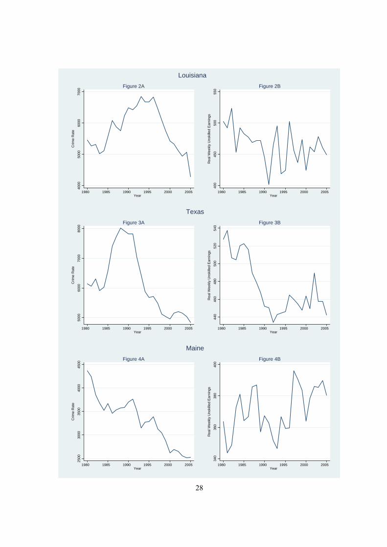
Figures 2A-7A display the crime rates of unskilled workers in a sample of states from

different regions of the country. There is significant heterogeneity in the behavior of the

crime rates. For example, over the sample period of 1980 to 2005, Louisiana’s crime rate

13

went up rather steadily between 1980 and 1996, and started declining afterwards. On the

other hand, the crime rate in Texas reached its peak in 1988, and the crime rate in Maine has

declined since 1980 with some jumps in late 1980s and mid 1990s. The crime rate in

California declined in the early 1980s, then remained steady for a decade, and dropped

significantly between 1993 and 1999. In contrast, crime went up between early 1980s and

early 1990s in Massachusetts before started declining, and the crime in West Virginia went

up, rather than decline, between early1980s and 2005.

Figures 2B-7B present the quality-adjusted real weekly earnings of unskilled workers

in the same states.8 In some states, there is a visible negative correlation between crime and

real weekly earnings of unskilled workers. For example, in Louisiana, earnings of unskilled

workers went down between 1980 and 1991, and they bounced and started going up after

1991. Crime in Louisiana increased between 1980 and 1996, and declined afterwards. In

Maine and West Virginia, real weekly earnings of unskilled workers were going up between

1980 and 2005 when crime was declining. Real earnings steadily declined in Texas between

1980 and 1992, and they started increasing afterwards. Crime in Texas exhibits the reverse

pattern. On the other hand, the correlation between crime and earnings of unskilled workers

is not strong in Massachusetts and in California.9 Note that Figures 2B-7B display quality-

adjusted real weekly earnings of unskilled workers (see the Appendix for the construction).

The level of simple weekly earnings (unadjusted for education, experience or gender

composition) are higher, but the two follow the same time-series pattern in a state. 8 The average weekly earnings for each year are calculated using weighted individual weekly earnings. 9 These particular states are not anomalies in any sense. Analysis of other states shows that the behavior of the crime rate is quite different between the states. For example, the crime rate in Florida increased steadily between 1984 and 2005, while Michigan exhibited a continuous decline in crime. Similarly, there is heterogeneity between states regarding the simple correlation between the crime rate and earnings of unskilled workers. For example, the two variables move in opposite direction in Mississippi over time, while the relationship is less clear in Indiana.

14

VII. Estimation Results of State-level Panel Data

Tables 2A and 2B present the instrumental variables results where aggregate property

crime, aggregate violent crime, and their components (i.e. burglary, larceny, murder, and so

on) are regressed on unskilled workers’ real earnings, arrests rates for the corresponding

crimes and other time-varying state attributes. Earnings of unskilled workers are

instrumented with ln( )H LA A from Equation (5). The instrument is powerful in each case,

and the F-statistic of the instrument in the first stage regressions is about 28. Regressions

also control for state and time fixed-effects and a common time-trend; the standard errors are

clustered at the state level. Following Levitt (1998), Corman and Mocan (2000), and Katz,

Levitt, and Shustorovich (2003), arrest rates are lagged once to minimize the impact of

simultaneity between crime and deterrence.

Column (1) of Table 2A shows that the IV-estimate of the coefficient of unskilled

(non-college) workers’ weekly earnings is about -10 in the total property crime regression

and it is highly significant. The estimate suggests that a $20 increase in weekly real earnings

of unskilled workers (which corresponds to a 5 % increase at the sample mean) reduces

property crime rate by 200 (or about 10,500 fewer property crimes in a state in a year), which

corresponds to a 4.8 % decline. This suggests an elasticity of property crime with respect to

real weekly earnings of -0.96. Columns (2) and (3) show that an increase in weekly earnings

of unskilled workers reduces two components of property crime: burglary and larceny, but it

has no impact on motor-vehicle theft. A $20 increase in weekly earnings of unskilled

workers generates a decline in the burglary rate by about 60, or 6%, which translates into

3,160 fewer burglaries. The same increase in earnings brings about a decline in the larceny

15

rate by 160, (5.7%). This suggests that the elasticity of burglary and larceny with respect of

the earnings of unskilled workers is in the range of -1.1 to -1.2. The coefficient of unskilled

workers’ earnings is not significantly different from zero in violent crime regressions.10

Table 2A also shows that state alcohol consumption is positively related to crime and

that the arrest rate has a negative impact on most crimes and the impact is estimated with

precision in case of burglary, larceny, and total property crime. Lagging the arrest rate twice

or omitting it from the models did not alter the estimated coefficients of weekly earnings.11

Per capita state income has a negative impact on motor vehicle thefts and robberies.

Table 2B displays the results of the instrumental variables regressions which include

Weekly Earnings+ and Weekly Earnings-- as two separate regressors. The first stage

regression of this specification uses ln( )H LA A + and ln( )H LA A − as instruments, which are

constructed the same way as Weekly Earnings+ and Weekly Earnings--. Column (1) of Table

2B shows that a decrease in unskilled workers’ weekly earnings has a larger impact on total

property crime than an increase in earnings by the same magnitude. That is, the coefficient

of Weekly Earnings-- is larger in absolute value than that of Weekly Earnings+, and the

difference is statistically different from zero at the eight percent level. Specifically, if real

weekly earnings of unskilled workers go down by $10, the property crime rate goes up by

about 176, which corresponds to an increase in the number of property crimes by about

10 Estimating the models using OLS, by treating the weekly earnings of unskilled workers as

exogenous, provided estimates of earnings that were mostly positive and sometimes statistically different from zero. At its face, this would suggest that an increase in weekly earning of non-college workers would increase crime, and it underlines the importance of addressing endogeneity. 11 In models that omitted the deterrence variables, estimated coefficients of weekly earnings were larger in absolute value in most cases.

16

9,275.12 On the other hand, if weekly earnings increase by $10, the property crime rate goes

down by only 168, which translates into a decline in the number of property crimes by 8,854.

The same asymmetry is detected in the impact of weekly earnings of unskilled workers on

burglary and larceny. In both cases, a decline in real weekly earnings has a larger impact on

criminal activity than an increase in weekly earnings by the same magnitude, although the

difference is not significantly different from zero in case of burglary (p=0.15).

Tables 3A and 3B present the results of similar analyses with one difference. In these

specifications, we employ real weekly earnings of unskilled men as opposed to all unskilled

workers. The results indicate that weekly earnings of unskilled men have a negative impact

on burglaries, larcenies and on overall property crime. Table 3B demonstrates that,

consistent with earlier results, a decline in weekly earnings of unskilled men generates a

larger impact on property crime than an increase by the same amount. (The coefficients of

Weekly Earnings-- are larger in absolute value than the coefficients of Weekly Earnings+, and

the difference between the estimated coefficients is different from zero in case of larceny and

it is borderline significant for total property crimes).

The framework of the skill-biased technological change depicted by Equations (4)

and (5) and the literature on wage inequality assume that wages are determined on inelastic

relative supply of the skill groups (Acemoglu and Autor 2010; Autor, Katz and Kearney,

2008; Autor, Katz, Krueger 1998). Deviations from full-employment are implicitly ruled out,

but they can take place idiosyncratically because of cyclical conditions. This suggests that

one can incorporate unemployment to this analysis as an exogenous variable as was done in

the analysis of wage inequality (e.g. Autor, Katz and Kearney 2008). Tables 4A-5B display 12 The coefficients of Weekly Earnings+ and Weekly Earnings— are larger in comparison to the coeffiients of Weekly Earnings reported in table 2B because the mean values of Weekly Earnings+ and Weekly Earnings— are smaller than Weekly Earnings by construction (see Equation 3).

17

the results of the models that include state unemployment rate as an additional explanatory

variable. A comparison with Tables 2A-3B shows that inclusion of the unemployment rate

does not alter the magnitudes of other coefficients appreciably and that unemployment has an

independent and positive effect on total property crime, and well as on burglaries and

larcenies. An increase in unemployment also increases robberies: a violent crime that has a

monetary motive. Tables 4A and 4B imply that a one-percentage point increase in the state

unemployment rate increases property crime rate by 74-103, (which translates into an

increase in property crimes by 2%), which generates 3,636 to 4,954 additional property

crimes per year. This magnitude is remarkably similar to the ones reported by recent

research. The same one-percentage point increase in the unemployment rate generates a 3.8%

increase in robberies. Consistent with earlier results, Tables 4B shows that the impact of

weekly earnings of low-skilled workers on crime is larger when earnings are declining.

These results also underline the importance of addressing endogeneity of earnings, as

OLS regressions (not reported) of crime on earnings revealed positive and insignificant

coefficients of earnings.

VIII. Analysis of Micro Data

Based on the theoretical framework summarized in Section III above, and following

Grogger (1998), in this section we estimate a structural crime participation equation using

data from NLSY97. Specifically, consider equations (6) and (7) below

(6) ln it it itW X ε= Ω+ ,

(7) ln[ ( )] ,cit it it cit itR T X D Tλ μ′ = Φ + Ψ + +

18

where (6) is a standard Mincerian equation for market wages W, and equation (7) specifies

the marginal returns to crime, where cT represents time spent committing crime, and

( )c cR T R T′ = ∂ ∂ stands for the returns to committing crime. X stands for the vector of

personal attributes and D stands for state characteristics, including deterrence variables.

As described in section III, if the person is engaged in crime, it should be the case that

ln[ ( 0)] lncitR T W′ > > . This indicates that the probability of committing crime [Pr(CR=1)]

can be depicted as Pr( 1) Pr( ln 0)CR X D Wμ= = Φ + Ψ + − > ) or

(8) Pr( 1) Pr( ln )it itCR W X Dμ= = > − Φ − Ψ .

Equation (8) can be estimated by maximum likelihood probit, but two complications exist.

First, market wages W are not observed for those who don’t work in the labor market, and

estimating Equation (8) using only those who work could produce sample selection bias.

Second, ε and μ in Equations (6) and (7) are likely to be correlated. That is, unobserved

factors that influence labor market productivity may be correlated with unobservables that

impact productivity in the criminal sector, which constitutes a potential source of

endogeneity of wages. To address the first issue, we specify a selection equation that

classifies individuals into worker vs. non-worker groups and estimates it along with the wage

equation using full maximum likelihood. Identification is achieved by including unearned

income in the selection equation and excluding it from the wage equation. Alternative

identification restrictions, such as including indicators of marijuana use and gun ownership in

addition to household income, provided the same results. This selectivity-corrected wage

equation is used to impute the market wages of non-workers.

To address the endogeneity of wages, we instrument wages with skill-biased

technological change index as explained in section V. Because each worker’s sector of work

19

is known in the data, we classified workers into three groups as working in the service sector,

in the manufacturing sector, or in other sectors (which consists of agriculture, mining and

construction). We calculated the index of skill-biased technology for each state, year, and

sector using the algorithm described in the Appendix. More specifically, we specified

production functions for the manufacturing sector, the sector, service sector and the residual

(all other) sectors which depend on skilled and unskilled labor as before and recovered the

index for the skill-biased technology using equation (5).

We then matched each worker in each state, year and sector with the corresponding

sector-state-and year specific skill-biased technology index. Because the sector affiliation is

unknown for non-workers, we matched them by year, with the state-and-year specific skill-

biased technology index—the one that is used in the state-panel analysis of the paper.

In this framework we estimate Equation (9) where ijtCR stands for an indicator of various

types of criminal activity (e.g. theft, stealing cars, drug sales) for person i who resides in state

j in time t, and the vector X stands for personal attributes of the person. D represents a vector

of time-varying state characteristics which includes aggregate measures of deterrence, such

as the arrest rates for specific crimes. ln ijtW is the logarithm of the market wages of worker i,

in state j and time t, instrumented with skill-biased technological change; and υ stands for the

error term:

(9) ln .cijt ijt ijt jt i ijtCR W X D tβ ε θ υ′ ′= + Φ+ Ψ + + +

20

IX. Micro Data from the NLSY97

We use confidential geo-coded National Longitudinal Survey of Youth 1997 cohort

(NLSY97). The main data set is constructed using information from the 1997 - 2003 waves

of the NLSY97, which contains a nationally representative sample of 8,984 youths who were

aged 12 to 16 as of December 31st 1996. The respondents have been followed annually since

the survey was initiated. We limit the sample to 1997-2003 waves because everyone who

took the survey between these years was asked of question on criminal activity. After 2003

crime questions were asked to those who had reported to have been arrested in previous

waves in addition to a small group of not-arrested respondents.

We employ seven different indicators of delinquency. They are robbery, which is a

violent crime, and six categories of property crimes such as whether the person committed

burglary, whether he/she stole a car, whether he/she sold or helped selling hard drugs like

cocaine, and whether he/she sold any drugs. Other crime measures include stealing a purse, a

wallet, or stealing something from a store (Larceny); and Other Property Crimes such as

whether the person received, possessed or sold stolen property, embezzlement, and fraud. We

also employ a variable to indicate if the person committed Larceny, Car Theft or Robbery. 13

In each wave, individuals are asked about the jobs they have taken since the last

interview. Respondents report up to 11 different jobs as well as the hourly compensation

they have received in each job. Highest hourly compensation reported for the year is used as

13 These outcome variables are constructed based on a series of questions in the following form “Have you done XXX since the last interview?” where XXX stands for various crimes mentioned in the text. From 1998-2003 all crime questions were asked in that form. In the first wave in 1997, the question was “Have you ever done XXX?” followed by “How many times have you committed XXX in the last 12 months?” or “How old were you when you last did XXX?” Thus, we used these variables to construct the outcome variables for the first wave.

21

the relevant wage (Finlay 2009). To eliminate outliers, above the 95th percentile of the wage

distribution are omitted. Finally, the wage rate is deflated by the State-level CPI.

Some of the individuals in our sample reported that they have not worked since the

date of last interview. Their market wages are predicted by estimating jointly a labor force

participation and equation and a wage equation as shown by Equations (8) and (9). The

exclusion restriction for the selection equation is to omit conventional non-labor income from

the wage equation. Non-labor income is defined as the difference between individual’s total

household income and his/her personal labor income. As a result, our non-labor income

measure includes the following income types: child support, interest from bank accounts,

dividends from stocks or mutual funds, rental income, income received from the parents, and

from other sources (except own farms/businesses or salaries).

NLSY97 includes information about the industry classifications of individuals’ jobs.

We used the 2002 Census definitions of the industries.14 After matching individuals with

their industries, we used the technology shocks as an instrumental variable. Obviously, those

individuals who reported not having worked since the date of the last interview do not belong

to an industry. Consequently, we modified our instrumental variable such that the non-

working people are matched with the overall technology shocks.

Individual control variables employed includes whether the individual has carried a gun in

the last year, individual’s age, an indicator for whether the individual has at least a high

school degree (including GED), individual’s household income (income from all sources in

the family) and household size, indicators for marital status, number of biological children

the individual has (regardless of whether they live in individual’s household), an indicator for

whether the individual lives in an urban area, and the number of days in the last month the 14 The Census Bureau has re-classified some of the jobs in 2002. We utilized this new classification.

22

individual has consumed more than 5 alcoholic beverages and used marijuana.15 In addition,

we use aggregate level control variables. These controls are the per capita personal income in

individual’s state, share of the population aged between fifteen and twenty four and share of

the population that is black in the state. Moreover, we matched the individuals in our sample

with the relevant arrest rates by their county and according to the crime they have committed

and whether they are older or younger than 18 years of age. For example, somebody who is

younger than 18 is matched with juvenile arrest rates and those with age greater than or equal

to 18 are matched with adult arrest rate in the county with the specific crimes.

County-level arrest data are obtained Uniform Crime Reporting Program (County-

Level Detailed Arrest and Offense Data sets for years between 1997 and 2004). These data

provide the number of juvenile and adult arrests in each county for several crime categories

including the Index I crimes and minor crimes such as drug sale, fraud, embezzlement,

vandalism and so on. Using the population of each county, we calculated per capita (times

100,000) adult and juvenile arrests for motor vehicle theft, robbery, larceny, and burglary.

For hard drugs, we used the arrests pertaining to the sale and manufacturing of cocaine and

opium; and for any drug we used the arrests pertaining to the sale and manufacturing of nay

narcotics. For Other property crime, we used the arrest rates for forgery, fraud,

embezzlement and buying/receiving/possessing stolen property. For Any Property Crime, we

used the sum of the property crime arrests and robbery arrests.

15 Urban classification has been changed in 2003 by the NLSY (because the Census classification was changed in 2000). We employed the definition as reported in the NLSY.

23

Table 5 presents the descriptive statistics. The regressions include the individuals

who have contributed at least two observations to the sample. The reported descriptive

statistics pertain to our largest sample – regressions for the ANY CRIME outcome. 16

X. Estimation Results using Micro Data

Table 6 presents the results obtained from estimation of the selection equation and the

market wage equation. The two equations are estimated jointly using maximum likelihood.

The results are consistent with those obtained from typical wage studies where having at least

a high school degree and being male have a positive impact on wages, but being Black has a

negative impact on wages in comparison to whites. State income and living in urban areas

are positively correlated with wages. Nonlabor income has a negative impact on the

propensity to work in the legal labor market; the same is true for state income and the

unemployment rate. Higher education makes the person more likely to participate in the

legal labor market. Blacks and Hispanic have lower propensities to participate.

Table 7A presents the crime regressions that employ the NLSY data. Potential

market wages of non-workers are imputed using the selection-corrected wage equation

16 The means of the county level arrest rates are smaller in comparison to the means of the state level arrest rates (reported in Table 1). This is because of three reasons. First, the sample includes individuals from small counties in which there are very few arrests for some crime types. This pulls the sample average down. Secondly, when calculating the arrest rates, we deflated the total number of arrests for each specific crime for both juveniles and adults with the total number of people in the jurisdiction covered by the agencies in the county. In other words, to calculate the juvenile (adult) arrest rate for, say, larceny, we divided the number of juvenile (adult) larceny arrests by the total population. Ideally, we would use the number of juveniles in the county to calculate the juvenile arrest rates and the number of adults to calculate the adult arrest rates. However, such information is not provided by the FBI. As a result, although our measures of the county arrest rates are good proxies for juvenile and adult arrests, they are lower than their true value. Thirdly and most importantly, our sample is mostly made up of young individuals. The average age is below eighteen. Consequently, the juvenile arrest rate has a greater weight in the means reported in Table 5. The juvenile arrests make up only a small portion of total arrests. For example, in 2004, only 16% of all arrests involved a juvenile in the US. Therefore, it is natural to have smaller means for the arrest rates in the individual level analysis.

24

displayed in Table 6 and wages are instrumented by state-year-sector specific skill-biased

technology parameters. Because non-workers’sector of work does not exist, we assigned

them the state-and-year specific skill-biased technology index.

Real wages have no significant impact on robbery or burglary,17 but they impact all

other crime categories. The results indicate that a 1-percent increase in real wages decreases

the propensity to steal something from a store or a purse or wallet (column 2) by about 16

percentage points. The same increase in wages generates a decline in the propensity to steal

a car by 4 percentage points. Similarly, wages have a negative impact on participating in

other crimes (possession of stolen property, etc.), selling any drugs, as well as selling hard

drugs. The implied elasticies are about -1.7 for most crime categories.

Arrests reduce criminal proclivity with statistically significant impacts in case of

larceny, selling hard drugs, burglary and the indicator that identifies whether the person

committed larceny, robbery or car theft. Heavy drinking, marijuana use and carrying a gun

are positively related to criminal activity.

Table 7B displays the model which includes Wage+ and Wage -- as explanatory

variables. Similar to the results obtained from state panels (see Table 2B), the coefficients of

Wage— are generally larger in absolute value than those of Wage+ indicating that the impact

on the propensity to commit crime of a given decrease in wages is larger than the increase in

wages of the same magnitude. The difference in the coefficients of Wage+ and Wage-- is

significantly different from zero in the models that explains selling hard drugs (column 6),

and where larceny+robbery+motor vehicle theft is the dependent variable (column 1). The

difference is marginally significant (p=0.12) in case of other crime (column 5). 17 Robbery is a violent crime, where the perpetrator takes or attempts to take something valuable from the victim by using a weapon or by the threat of violence. Burglary involves entering into a structure, such as a house, to commit theft.

25

The results obtained from estimating the models for men are presented in Tables 8A

and 8B. Wages have a negative and statistically significant impact on all crimes with the

exception of robbery and burglary. Table 8B shows that the impact of Wage— is larger than

that of Wage+ as before ,and that the difference in the impact is significantly different from

zero in case of larceny (column 2) and larceny-robbery-motor vehicle theft (column 1).

XI. Conclusion

Although formal economic models of crime were developed more than four decades

ago, empirical issues have created substantial obstacles regarding reliable inference about the

magnitudes of the relationships between economic variables and criminal activity.

Inconsistent estimates reported in the literature prompted some analysts to argue that there is

little evidence to support the hypothesis that economic conditions impact crime and that there

is a disconnect between theory and empirical evidence (Piehl 1998). In this paper we

investigate the impact of unskilled (non-college educated) workers earnings in crime. Using

the framework employed in the literature on wage inequality, and using the March CPS data,

we create a state-and-year specific measure of skill-biased technological change and use it as

an instrument for unskilled workers’ earnings in state panels.

Estimation of crime regressions using state panels from 1980 to 2005 demonstrate

that a decrease in unskilled workers real weekly earnings, induced by skilled-biased

technological change, is negatively elated to state property crime with an elasticity of -1.0

Violent crime is not influenced by weekly earnings of unskilled workers. We also detect

asymmetry in the impact of unskilled workers earnings on crime. A deterioration in earnings

has a larger effect on crime in magnitude in comparison to an increase in earnings by the

26

same absolute amount. We find that the earnings of non-college educated males are related

to crime, but the earnings of unskilled females have no impact on criminal activity.

We also employ micro data from the geocoded confidential version of the NLSY97 to

estimate models of criminal participation. The NLSY97 data contain detailed measures of

individuals’ criminal activity as well as personal and household attributes and wages.

Goecodes allow us to identify the location of the individual and merge them with the relevant

county arrest rates. The data set consists of young and mostly unskilled workers. For those

who have not participated in the legal labor market, we impute wages by jointly estimating a

labor force participation equation and a wage equation. We create state-year-industry

specific measures of skill-biased technological change for three broad industry categories

(manufacturing, service, other) and match workers with the relevant skill-biased

technological change indicators, by their industry.18 We instrument market wages with

state-year-industry specific technology shocks and find wage elasticities in the range of -1.7

for property crimes such as larceny and car theft. The asymmetric impact of wages on crime

is also detected in micro data.

The results indicate that individual crime decisions respond to labor market

incentives as predicted by theory, and that an increase in wages of unskilled workers has a

significant impact on criminal activity.

18 Those who have not worked in the labor market in a given year, are matched the with state-wide technology shock in that year.

27

Figure 1 U.S. Crime

3500

4000

4500

5000

5500

6000

Offe

nses

per

100

,000

resi

dent

s

1980 1985 1990 1995 2000 2005Year

Total Crime Rate Property Crime Rate

28

4000

5000

6000

7000

Crim

e R

ate

1980 1985 1990 1995 2000 2005Year

Figure 2A

400

450

500

550

Rea

l Wee

kly

Uns

kille

d Ea

rnin

gs

1980 1985 1990 1995 2000 2005Year

Figure 2B

Louisiana50

0060

0070

0080

00

Crim

e R

ate

1980 1985 1990 1995 2000 2005Year

Figure 3A

440

460

480

500

520

540

Rea

l Wee

kly

Uns

kille

d Ea

rnin

gs

1980 1985 1990 1995 2000 2005Year

Figure 3B

Texas

2500

3000

3500

4000

4500

Crim

e R

ate

1980 1985 1990 1995 2000 2005Year

Figure 4A

340

360

380

400

Rea

l Wee

kly

Uns

kille

d Ea

rnin

gs

1980 1985 1990 1995 2000 2005Year

Figure 4B

Maine

29

4000

5000

6000

7000

8000

Crim

e R

ate

1980 1985 1990 1995 2000 2005Year

Figure 5A

350

400

450

Rea

l Wee

kly

Uns

kille

d Ea

rnin

gs

1980 1985 1990 1995 2000 2005Year

Figure 5B

California 30

0040

0050

0060

00

Crim

e R

ate

1980 1985 1990 1995 2000 2005Year

Figure 6A

340

360

380

400

Rea

l Wee

kly

Uns

kille

d Ea

rnin

gs

1980 1985 1990 1995 2000 2005Year

Figure 6B

Massachusetts

2200

2400

2600

2800

3000

Crim

e R

ate

1980 1985 1990 1995 2000 2005Year

Figure 7A

360

380

400

420

440

460

Rea

l Wee

kly

Uns

kille

d Ea

rnin

gs

1980 1985 1990 1995 2000 2005Year

Figure 7B

West Virginia

30

Table 1: Descriptive Statistics

(State Panels, 1980-2005)

Variable Mean Std. Dev. Weekly Earnings-Unskilled Simple Average All Unskilled Workers 679.9 (63.9) Male Unskilled Workers 778.6 (81.7) Quality Adjusted All Unskilled Workers 410.1 (41.8) Male Unskilled Workers 408.1 (44.8) Crime Rates Property 4,149.5 (1,102.2) Burglary 949.3 (359.5) Larceny 2,796.3 (699.6) Motor Vehicle Theft 404.0 (210.6) Violent 470.3 (238.0) Murder 6.0 (3.4) Rape 36.0 (13.8) Robbery 133.6 (96.4) Assault 294.6 (154.5) Arrest Rates Property 14.57 (227.28) Burglary 2.27 (30.3) Larceny 11.5 (188.6) Motor Vehicle Theft 0.8 (8.4) Violent 2.63 (20.9) Murder 0.08 (0.8) Rape 0.26 (4.2) Robbery 0.56 (5.4) Assault 1.7 (10.5) Income Per Capita 22,085.1 (7,161.5) Unemployment Rate 5.7 (1.9) Percent 15-24 Year Olds 14.9 (1.5) Percent Black 10.0 (9.4) Percent Urban Population 71.2 (14.7) Alcohol Consumption 2,324.4 (389.9)

Notes: The crime rates are per 100,000 state population covered by the police agencies that report to FBI. Arrest rate is calculated as the number of arrests per 1,000 population. Criminal Justice Expenditures is total justice expenditures (state and local) per 100,000 population. Alcohol consumption is volume of beer consumption (in 1,000 gallons) per 100,000 population.

31

Table 2A Instrumental Variable State Panel Regressions

The Impact of Unskilled Weekly Earnings on Crime Property Violent Total Burglary Larceny MV Theft Total Murder Rape Robbery Assault I II III IV V VI VII VIII IX Weekly Earnings-Unskilled -9.933** -3.018** -8.090*** 1.171 -0.284 -0.002 -0.056 -0.100 -0.136 (3.983) (1.429) (2.660) (1.084) (0.504) (0.009) (0.060) (0.264) (0.330) Income Per Capita -0.047 -0.010 -0.003 -0.034*** -0.009 0.000 0.000 -0.006** -0.002 (0.034) (0.010) (0.021) (0.011) (0.006) (0.000) (0.000) (0.003) (0.004) Arrest Rate (-1) -0.089*** -0.188*** -0.072*** -0.031 -0.029 -0.002 0.015 0.016 -0.024 (0.018) (0.055) (0.014) (0.155) (0.034) (0.016) (0.014) (0.102) (0.062) Percent 15-24 Year Olds -41.409 -10.188 -53.929** 22.739** 0.450 0.256*** 1.170** -1.071 0.145 (44.037) (15.605) (26.738) (11.414) (6.647) (0.065) (0.575) (2.761) (6.188) Percent Black 97.790 18.051 58.560 21.205 12.731 0.469** -1.369 2.298 11.471 (82.820) (30.568) (48.324) (19.881) (16.820) (0.203) (1.318) (7.891) (10.091) Alcohol Consumption 1.634*** 0.476*** 1.060*** 0.099 0.190*** 0.002*** 0.013*** 0.082*** 0.093*** (0.312) (0.102) (0.197) (0.080) (0.047) (0.001) (0.004) (0.024) (0.033) Observations 1111 1111 1111 1111 1111 1111 1111 1109 1111 Robust Standard errors, clustered at the state level are in parentheses. * signifies statistical significance at the 10% level; ** at 5% level, and *** at the 1% level or less. The dependent variable for each regression is the crime rate per 100,000 state population covered by the police agencies that report to FBI. Arrest rate is calculated as the number of arrests per 1,000 population. Alcohol consumption is volume of beer consumption (in 1,000 gallons) per 100,000 population. The regression also includes percent urban population.

32

Table 2B

Instrumental Variable State Panel Regressions The Impact of Unskilled Weekly Earnings (Increase and Decrease) on Crime

Property Violent Total Burglary Larceny MV Theft Total Murder Rape Robbery Assault I II III IV V VI VII VIII IX Weekly Earnings-Unskilled(+) -16.822** -5.162* -14.758*** 3.092 0.222 -0.011 -0.065 0.335 -0.036 (7.863) (2.832) (5.710) (2.296) (0.992) (0.020) (0.128) (0.492) (0.680) Weekly Earnings-Unskilled(-) -17.627** -5.413* -15.537** 3.317 0.282 -0.013 -0.066 0.386 -0.024 (8.289) (2.985) (6.037) (2.442) (1.062) (0.022) (0.136) (0.527) (0.726) Income Per Capita -0.022 -0.002 0.021 -0.041*** -0.010 0.000 0.000 -0.008** -0.003 (0.045) (0.014) (0.031) (0.013) (0.008) (0.000) (0.001) (0.004) (0.004) Arrest Rate (-1) -0.086*** -0.181*** -0.068*** -0.055 -0.031 -0.001 0.015 0.005 -0.024 (0.020) (0.058) (0.016) (0.149) (0.033) (0.016) (0.012) (0.096) (0.061) Percent 15-24 Year Olds -58.860 -15.620 -70.821* 27.609** 1.734 0.231*** 1.147* 0.030 0.399 (53.950) (18.937) (36.590) (13.473) (7.181) (0.086) (0.652) (3.094) (6.630) Percent Black 116.533 23.884 76.703 15.977 11.352 0.495** -1.344 1.113 11.198 (95.336) (34.645) (63.567) (23.115) (15.635) (0.226) (1.459) (7.203) (9.799) Alcohol Consumption 1.789*** 0.524*** 1.209*** 0.056 0.178*** 0.002** 0.014*** 0.072*** 0.091** (0.399) (0.131) (0.274) (0.094) (0.049) (0.001) (0.005) (0.024) (0.037) Observations 1111 1111 1111 1111 1111 1111 1111 1109 1111 Robust Standard errors, clustered at the state level are in parentheses. * signifies statistical significance at the 10% level; ** at 5% level, and *** at the 1% level or less. The dependent variable for each regression is the crime rate per 100,000 state population covered by the police agencies that report to FBI. Arrest rate is calculated as the number of arrests per 1,000 population. Alcohol consumption is volume of beer consumption (in 1,000 gallons) per 100,000 population. The regression also includes percent urban population.

33


The Impact of Male Unskilled Weekly Earnings on Crime

Property Violent Total Burglary Larceny MV Theft Total Murder Rape Robbery Assault I II III IV V VI VII VIII IX Weekly Earnings-Unskilled -8.452** -2.568** -6.883*** 0.996 -0.242 -0.001 -0.047 -0.085 -0.116 (3.347) (1.223) (2.234) (0.934) (0.423) (0.008) (0.050) (0.223) (0.278) Income Per Capita -0.047 -0.010 -0.003 -0.034*** -0.009 0.000 0.000 -0.006** -0.002 (0.033) (0.010) (0.021) (0.011) (0.006) (0.000) (0.000) (0.003) (0.004) Arrest Rate (-1) -0.098*** -0.208*** -0.080*** -0.003 -0.031 -0.003 0.012 0.013 -0.026 (0.021) (0.062) (0.016) (0.181) (0.037) (0.017) (0.016) (0.104) (0.064) Percent 15-24 Year Olds -37.277 -8.932 -50.564* 22.252** 0.568 0.257*** 1.193** -1.030 0.201 (43.575) (15.457) (26.270) (11.192) (6.586) (0.064) (0.557) (2.762) (6.112) Percent Black 89.333 15.481 51.672 22.203 12.489 0.467** -1.416 2.208 11.355 (79.946) (29.376) (47.219) (19.984) (16.745) (0.201) (1.283) (7.852) (10.063) Alcohol Consumption 1.619*** 0.471*** 1.047*** 0.101 0.189*** 0.002*** 0.013*** 0.082*** 0.093*** (0.303) (0.100) (0.193) (0.080) (0.046) (0.001) (0.004) (0.024) (0.032) Observations 1111 1111 1111 1111 1111 1111 1111 1109 1111 Robust Standard errors, clustered at the state level are in parentheses. * signifies statistical significance at the 10% level; ** at 5% level, and *** at the 1% level or less. The dependent variable for each regression is the crime rate per 100,000 state population covered by the police agencies that report to FBI. Arrest rate is calculated as the number of arrests per 1,000 population. Alcohol consumption is volume of beer consumption (in 1,000 gallons) per 100,000 population. The regression also includes percent urban population.

34

Table 3B Instrumental Variable State Panel Regressions

The Impact of Unskilled Male Weekly Earnings (Increase and Decrease) on Crime

Property Violent Total Burglary Larceny MV Theft Total Murder Rape Robbery Assault I II III IV V VI VII VIII IX Weekly Earnings-Unskilled(+) -12.653** -3.882* -11.094*** 2.319 0.163 -0.009 -0.049 0.250 -0.028 (5.750) (2.092) (4.106) (1.679) (0.770) (0.015) (0.095) (0.386) (0.512) Weekly Earnings-Unskilled(-) -13.366** -4.106* -11.809*** 2.543 0.232 -0.010 -0.049 0.307 -0.013 (6.151) (2.238) (4.408) (1.814) (0.842) (0.016) (0.103) (0.424) (0.558) Income Per Capita -0.033 -0.006 0.011 -0.038*** -0.010 0.000 0.000 -0.007** -0.003 (0.038) (0.011) (0.026) (0.012) (0.007) (0.000) (0.000) (0.004) (0.004) Arrest Rate (-1) -0.100*** -0.213*** -0.083*** 0.014 -0.029 -0.004 0.012 0.019 -0.025 (0.023) (0.069) (0.019) (0.186) (0.039) (0.019) (0.017) (0.106) (0.066) Percent 15-24 Year Olds -55.258 -14.558 -68.586** 27.913** 2.301 0.226*** 1.186* 0.406 0.577 (51.972) (18.108) (34.125) (12.552) (7.226) (0.087) (0.634) (3.174) (6.597) Percent Black 102.580 19.626 64.950 18.033 11.213 0.490** -1.411 1.167 11.078 (86.446) (30.881) (57.073) (22.171) (16.667) (0.217) (1.387) (7.943) (9.989) Alcohol Consumption 1.738*** 0.508*** 1.166*** 0.063 0.178*** 0.002*** 0.013*** 0.073*** 0.090** (0.355) (0.119) (0.238) (0.092) (0.048) (0.001) (0.005) (0.024) (0.036) Observations 1111 1111 1111 1111 1111 1111 1111 1109 1111 Robust Standard errors, clustered at the state level are in parentheses. * signifies statistical significance at the 10% level; ** at 5% level, and *** at the 1% level or less. The dependent variable for each regression is the crime rate per 100,000 state population covered by the police agencies that report to FBI. Arrest rate is calculated as the number of arrests per 1,000 population. Alcohol consumption is volume of beer consumption (in 1,000 gallons) per 100,000 population. The regression also includes percent urban population.

35


The Impact of Unskilled Weekly Earnings on Crime; Model with the Unemployment Rate Property Violent Total Burglary Larceny MV Theft Total Murder Rape Robbery Assault I II III IV V VI VII VIII IX Weekly Earnings-Unskilled -9.849** -2.991** -8.039*** 1.176 -0.279 -0.002 -0.055 -0.094 -0.137 (3.885) (1.408) (2.604) (1.077) (0.499) (0.009) (0.059) (0.256) (0.329) Income Per Capita -0.043 -0.009 -0.000 -0.033*** -0.008 0.000 0.000 -0.006** -0.003 (0.034) (0.010) (0.021) (0.011) (0.006) (0.000) (0.000) (0.003) (0.004) Arrest Rate (-1) -0.088*** -0.186*** -0.071*** -0.029 -0.028 -0.002 0.015 0.018 -0.024 (0.018) (0.053) (0.013) (0.153) (0.034) (0.016) (0.013) (0.100) (0.061) Unemployment 74.090*** 24.408*** 44.765** 4.926 4.482 -0.003 0.187 5.243*** -0.910 (27.973) (9.098) (17.465) (6.053) (3.956) (0.074) (0.369) (1.799) (2.798) Percent 15-24 Year Olds -25.051 -4.800 -44.046* 23.827** 1.440 0.255*** 1.211** 0.085 -0.056 (41.814) (14.792) (25.305) (10.975) (6.671) (0.069) (0.576) (2.650) (6.032) Percent Black 94.751 17.050 56.723 21.003 12.547 0.469** -1.376 2.084 11.508 (78.522) (29.520) (46.326) (19.486) (16.468) (0.203) (1.315) (7.480) (10.135) Alcohol Consumption 1.767*** 0.520*** 1.140*** 0.108 0.198*** 0.002*** 0.014*** 0.092*** 0.091*** (0.324) (0.105) (0.206) (0.086) (0.050) (0.001) (0.004) (0.026) (0.035) Observations 1111 1111 1111 1111 1111 1111 1111 1109 1111 Robust Standard errors, clustered at the state level are in parentheses. * signifies statistical significance at the 10% level; ** at 5% level, and *** at the 1% level or less. The dependent variable for each regression is the crime rate per 100,000 state population covered by the police agencies that report to FBI. Arrest rate is calculated as the number of arrests per 1,000 population. Alcohol consumption is volume of beer consumption (in 1,000 gallons) per 100,000 population. The regression also includes percent urban population.

36

Table 4B Instrumental Variable State Panel Regressions

The Impact of Unskilled Weekly Earnings (Increase and Decrease) on Crime Model with the Unemployment Rate

Property Violent Total Burglary Larceny MV Theft Total Murder Rape Robbery Assault I II III IV V VI VII VIII IX Weekly Earnings-Unskilled(+) -16.349** -5.009* -14.422*** 3.076 0.233 -0.011 -0.064 0.351 -0.042 (7.407) (2.706) (5.388) (2.255) (0.971) (0.020) (0.125) (0.478) (0.669) Weekly Earnings-Unskilled(-) -17.113** -5.246* -15.172*** 3.299 0.293 -0.012 -0.065 0.403 -0.031 (7.804) (2.850) (5.695) (2.397) (1.039) (0.021) (0.133) (0.513) (0.714) Income Per Capita -0.017 -0.001 0.024 -0.041*** -0.010 0.000 0.000 -0.008** -0.003 (0.042) (0.013) (0.030) (0.013) (0.008) (0.000) (0.001) (0.004) (0.005) Arrest Rate (-1) -0.084*** -0.178*** -0.067*** -0.056 -0.031 -0.001 0.015 0.005 -0.025 (0.019) (0.055) (0.015) (0.146) (0.033) (0.016) (0.012) (0.095) (0.061) Unemployment 103.029*** 33.394*** 73.185*** -3.532 2.203 0.040 0.224 3.262 -1.334 (37.337) (12.450) (25.024) (10.076) (5.333) (0.092) (0.568) (2.335) (3.642) Percent 15-24 Year Olds -35.210 -7.955 -54.021* 26.798** 2.240 0.240*** 1.198* 0.778 0.093 (48.385) (16.856) (32.387) (12.170) (6.892) (0.082) (0.611) (2.866) (6.256) Percent Black 111.336 22.199 73.011 16.155 11.241 0.493** -1.355 0.949 11.265 (88.100) (32.794) (58.791) (22.982) (15.474) (0.224) (1.444) (6.974) (9.868) Alcohol Consumption 1.966*** 0.581*** 1.335*** 0.050 0.182*** 0.002** 0.014** 0.078*** 0.088** (0.415) (0.136) (0.283) (0.106) (0.054) (0.001) (0.006) (0.026) (0.041) Observations 1111 1111 1111 1111 1111 1111 1111 1109 1111 Robust Standard errors, clustered at the state level are in parentheses. * signifies statistical significance at the 10% level; ** at 5% level, and *** at the 1% level or less. The dependent variable for each regression is the crime rate per 100,000 state population covered by the police agencies that report to FBI. Arrest rate is calculated as the number of arrests per 1,000 population. Alcohol consumption is volume of beer consumption (in 1,000 gallons) per 100,000 population. The regression also includes percent urban population.

37

Table 5: Descriptive Statistics: NLSY97 Data Definition Mean (STD) Crime Variables Larceny/CarTheft/Robbery =1 if stole something (property crimes and robberies), =0 otherwise 0.099 (0.299) Larceny =1 if stole something from a store or stole a purse/wallet, =0 otherwise 0.088 (0.283) Car Theft =1 if stole something from a store, =0 otherwise 0.007 (0.086) Other Crime =1 if possessed stolen goods, committed fraud, embezzlement ,etc. =0 otherwise 0.030 (0.171) Selling Drug =1 if sold any kind of drugs, =0 otherwise 0.058 (0.235) Selling Hard Drug =1 if sold hard drugs like cocaine, =0 otherwise 0.021 (0.144) Burglary =1 if went into a house or building to steal something, =0 otherwise 0.012 (0.110) Robbery =1 if used or threatened to use a weapon to get something from someone else,

=0 otherwise 0.004 (0.062)

Personal Variables Wage Real weekly wage in cents 949.753 (346.412) High School+ =1 if the respondent completed at least high school, =0 otherwise 0.390 (0.488) Household Income Annual household income in 1,000 dollars 26.416 (45.079) Non-labor Income Non-labor income in dollars in 100 dollars 5.093 (168.970) Household Size The number of individuals in the respondent’s household 4.145 (1.674) Age Age of the respondent 17.710 (2.583) Gun =1 if the respondent has carried a gun since the last interview, =0 otherwise 0.050 (0.218) Heavy Drinking The number of days in the last month that the respondent has consumed 5+

alcoholic beverages 1.079 (3.075)

Marijuana Use The number of days in the last month that the respondent has used Marijuana 1.703 (5.884) Urban =1 if the respondent lives in an urban area, =0 otherwise 0.739 (0.439) Married =1 if married, =0 otherwise 0.037 (0.189) Separated =1 if separated, =0 otherwise 0.002 (0.045) Children The number of children of the respondent 0.133 (0.435) County Variables Arrest:Larceny/CarTheft/Robbery The number of arrests of relevant age group (juveniles or adults) for stealing

(property crimes and robberies) per 1,000 people in respondent’s county 3.024 (2.042)

Arrest: Larceny The number of arrests of relevant age group (juveniles or adults) for larceny per 1,000 people in the respondent’s county

2.214 (1.618)

Arrest: Car Theft The number of arrests of relevant age group (juveniles or adults) for stealing a 0.270 (0.280)

38

car per 1,000 people in the respondent’s county

(Table 1 concluded) Arrest: Stolen Property etc. The number of arrests of relevant age group (juveniles or adults) for committing

other property crimes per 1,000 people in the respondent’s county 7.901 (16.828)

Arrest: Selling Drugs The number of arrests of relevant age group (juveniles or adults) for selling drugs per 1,000 people in the respondent’s county

0.543 (1.007)

Arrest: Selling Hard Drug The number of arrests of relevant age group (juveniles or adults) for selling hard drugs like cocaine per 1,000 people in the respondent’s county

0.284 (0.805)

Arrest: Burglary The number of arrests of relevant age group (juveniles or adults) burglary per 100,000 people in the respondent’s county

0.539 (0.428)

Arrest: Robbery The number of arrests of relevant age group (juveniles or adults) for robbery per

100,000 people in the respondent’s country 0.223 (0.241)

State Variables State Per Capita Income State Per Capita Income in 1,000 dollars 29.088 (4.415) Share of Population aged 15-24 Share of the Population for aged 15 to 24 14.041 (0.911) Share of Black population Share of Black population 13.403 (8.512)

39

Table 6 NLSY Data; Selection into Labor Force and Market Wages

Selection Equation Wage Equation Non Labor Income -0.0001** (0.00005) Household Size -0.001 -0.007*** (0.005) (0.002) High/College 0.089*** 0.071*** (0.022) (0.007) Male 0.014 0.047*** (0.016) (0.006) Black -0.272*** -0.022*** (0.022) (0.008) Hispanic -0.131*** -0.009 (0.024) (0.008) Age 0.181*** 0.023*** (0.008) (0.003) Urban -0.017 0.029*** (0.020) (0.007) Married -0.235*** 0.072*** (0.044) (0.014) Separated -0.076 -0.073 (0.155) (0.075) Divorced -0.345** 0.025 (0.146) (0.041) Children -0.160*** 0.013* (0.022) (0.007) State Per Capita Income -0.026 0.016** (0.017) (0.007) Unemployment -0.040** 0.009 (0.019) (0.007) Share of Population aged 15-24 -0.081** 0.034** (0.035) (0.013) Share of Black population -0.059* 0.030* (0.035) (0.015) Observations 55,037 rho -0.811

Robust standard errors, clustered at the individual level, are in parentheses. * signifies statistical significance at the 10% level; ** at 5% level, and *** at the 1% level or less. State alcohol consumption, state and year

dummies are included in all regressions.

40

Table 7A: NLSY Data. Instrumental Variables Regressions.

Robust standard errors, clustered at the individual level, are in parentheses. * signifies statistical significance at the 10% level; ** at 5% level, and *** at the 1% level or less. Urban, marital status, number of children, share of population aged 15-24, share of black population, state and year dummies are included in all regressions.

Larceny/

Car Theft/ Robbery

Larceny Car Theft Stolen Property etc. Selling Drugs Selling Hard

Drug Burglary Robbery

(1) (2) (3) (4) (5) (6) (7) (8) Log Wage -0.179*** -0.160*** -0.041*** -0.086*** -0.101** -0.058** -0.019 0.011 (0.048) (0.047) (0.016) (0.031) (0.040) (0.023) (0.021) (0.013) Arrest -0.002** -0.003** -0.008** -0.000 -0.000 0.002 -0.007*** -0.003 (0.001) (0.001) (0.003) (0.000) (0.002) (0.001) (0.002) (0.003) High School + -0.002 -0.005 0.005* 0.001 -0.008 -0.003 0.002 -0.001 (0.007) (0.007) (0.002) (0.004) (0.005) (0.003) (0.003) (0.002) Household Income 0.000 -0.000 0.000 0.000 -0.000 0.000 -0.000** -0.000 (0.000) (0.000) (0.000) (0.000) (0.000) (0.000) (0.000) (0.000) Household Size -0.000 0.002 -0.001 0.001 -0.000 -0.000 0.001 0.001 (0.002) (0.002) (0.001) (0.001) (0.001) (0.001) (0.001) (0.000) Age -0.016*** -0.013*** -0.001 -0.003 -0.002 -0.001 -0.003** -0.001* (0.003) (0.003) (0.001) (0.002) (0.002) (0.002) (0.001) (0.001) Gun 0.098*** 0.086*** 0.042*** 0.087*** 0.094*** 0.063*** 0.053*** 0.036*** (0.009) (0.010) (0.005) (0.007) (0.009) (0.007) (0.006) (0.005) Heavy Drinking 0.003*** 0.002*** 0.001*** 0.002*** 0.005*** 0.003*** 0.002*** 0.001** (0.001) (0.001) (0.000) (0.000) (0.001) (0.000) (0.000) (0.000) Marijuana Use 0.003*** 0.003*** 0.000 0.002*** 0.011*** 0.003*** 0.001** 0.000** (0.000) (0.000) (0.000) (0.000) (0.000) (0.000) (0.000) (0.000) State Per -0.004 -0.003 -0.001 -0.001 0.000 -0.001 -0.002* 0.000 Capita Income (0.003) (0.003) (0.001) (0.002) (0.002) (0.001) (0.001) (0.000) Observations 54,411 47,479 47,479 54,398 54,386 54,382 47,479 54,658

41

Table 7B: NLSY Data. Instrumental Variables Regressions, Wage Increase & Wage Decrease

Larceny/

Car Theft/ Robbery



(1) (2) (3) (4) (5) (6) (7) (8) Log Wage (+) -0.284*** -0.155 -0.052 -0.114* -0.056 -0.146*** -0.003 0.022 (0.108) (0.095) (0.033) (0.068) (0.083) (0.052) (0.039) (0.028) Log Wage (--) -0.301*** -0.165 -0.053 -0.122* -0.058 -0.156*** -0.003 0.022 (0.116) (0.101) (0.035) (0.072) (0.088) (0.056) (0.041) (0.029) Arrest -0.004* -0.004 -0.004 -0.000 -0.001 -0.001 -0.002 -0.001 (0.002) (0.002) (0.004) (0.000) (0.002) (0.001) (0.001) (0.005) High School + -0.009 -0.012** 0.003 -0.003 -0.010** -0.005 0.001 -0.001 (0.006) (0.006) (0.002) (0.004) (0.005) (0.003) (0.003) (0.002) Household Income 0.000 0.000 0.000* 0.000 -0.000 0.000 0.000 -0.000 (0.000) (0.000) (0.000) (0.000) (0.000) (0.000) (0.000) (0.000) Household Size -0.002 -0.000 -0.001 0.000 0.001 -0.001 0.000 0.001 (0.002) (0.002) (0.001) (0.001) (0.001) (0.001) (0.001) (0.001) Age -0.020*** -0.019*** -0.001 -0.005** -0.005 0.000 -0.005*** -0.001 (0.005) (0.004) (0.001) (0.003) (0.003) (0.002) (0.002) (0.001) Gun 0.095*** 0.077*** 0.031*** 0.081*** 0.097*** 0.060*** 0.043*** 0.035*** (0.011) (0.011) (0.005) (0.009) (0.010) (0.008) (0.007) (0.005) Heavy Drinking 0.003*** 0.002*** 0.001** 0.002*** 0.004*** 0.003*** 0.001*** 0.000 (0.001) (0.001) (0.000) (0.000) (0.001) (0.000) (0.000) (0.000) Marijuana Use 0.003*** 0.003*** 0.000 0.001*** 0.010*** 0.002*** 0.000** 0.000 (0.000) (0.000) (0.000) (0.000) (0.000) (0.000) (0.000) (0.000) State Per -0.008** -0.007* -0.001 -0.001 0.002 0.002 -0.001 -0.000 Capita Income (0.004) (0.004) (0.001) (0.002) (0.003) (0.002) (0.001) (0.001) Observations 43,043 36,565 36,566 43,041 43,028 43,025 36,566 43,234 Standard errors, clustered at the individual level, are in parentheses. * signifies statistical significance at the 10% level; ** at 5% level, and *** at the 1% level or less. Urban, marital status, number of children, share of population aged 15-24, share of black population, state and year dummies are included in all regressions.

42

Table 8A: NLSY Data. Instrumental Variables Regressions – Men.

Larceny/

Car Theft/ Robbery



(1) (2) (3) (4) (5) (6) (7) (8) Log Wage -0.197*** -0.162** -0.048** -0.092* -0.141** -0.088** -0.014 0.013 (0.070) (0.065) (0.023) (0.049) (0.061) (0.036) (0.033) (0.020) Arrest -0.002 -0.003 -0.014** -0.000 -0.002 0.004 -0.012*** -0.003 (0.002) (0.002) (0.006) (0.000) (0.003) (0.002) (0.004) (0.006) High School + 0.002 -0.003 0.005 -0.009 -0.009 -0.002 0.004 -0.002 (0.010) (0.010) (0.004) (0.007) (0.009) (0.006) (0.005) (0.003) Household Income 0.000 -0.000 0.000 -0.000 -0.000 0.000 -0.000*** -0.000 (0.000) (0.000) (0.000) (0.000) (0.000) (0.000) (0.000) (0.000) Household Size 0.001 0.004* -0.001 0.003** 0.001 -0.002* 0.002 0.001 (0.002) (0.003) (0.001) (0.002) (0.002) (0.001) (0.001) (0.001) Age -0.026*** -0.022*** -0.001 -0.007** -0.001 -0.002 -0.005** -0.001 (0.005) (0.005) (0.002) (0.003) (0.004) (0.003) (0.002) (0.001) Gun 0.091*** 0.078*** 0.038*** 0.080*** 0.087*** 0.059*** 0.048*** 0.037*** (0.010) (0.010) (0.006) (0.008) (0.009) (0.007) (0.007) (0.005) Heavy Drinking 0.003*** 0.002** 0.001*** 0.002*** 0.004*** 0.003*** 0.002*** 0.001*** (0.001) (0.001) (0.000) (0.001) (0.001) (0.001) (0.001) (0.000) Marijuana Use 0.003*** 0.002*** 0.000 0.002*** 0.011*** 0.002*** 0.000 0.000* (0.001) (0.001) (0.000) (0.000) (0.001) (0.000) (0.000) (0.000) State Per -0.001 0.003 -0.000 -0.000 0.001 -0.001 -0.003 0.001 Capita Income (0.004) (0.005) (0.002) (0.003) (0.003) (0.002) (0.002) (0.001) Observations 27,428 23,987 23,987 27,415 27,410 27,407 23,987 27,567 Standard errors, clustered at the individual level, are in parentheses. * signifies statistical significance at the 10% level; ** at 5% level, and *** at the 1% level or less. Urban, marital status, number of children, share of population aged 15-24, share of black population, state and year dummies are included in all regressions.

43

Table 8B: NLSY Data. Instrumental Variables Regressions—Men. Wage Increase & Wage Decrease

Larceny/

Car Theft/ Robbery



(1) (2) (3) (4) (5) (6) (7) (8) Log Wage (+) -0.335** -0.246* -0.066 -0.095 -0.042 -0.172** -0.003 0.016 (0.147) (0.127) (0.047) (0.098) (0.115) (0.073) (0.055) (0.038) Log Wage (--) -0.355** -0.266* -0.067 -0.101 -0.041 -0.181** -0.002 0.017 (0.157) (0.136) (0.050) (0.105) (0.123) (0.078) (0.058) (0.040) Arrest -0.003 -0.004 -0.008 -0.000 -0.002 0.001 -0.003 -0.003 (0.003) (0.003) (0.008) (0.000) (0.005) (0.003) (0.002) (0.008) High School + -0.004 -0.011 0.005 -0.008 -0.015* -0.006 0.003 -0.002 (0.010) (0.009) (0.004) (0.007) (0.008) (0.006) (0.005) (0.003) Household Income 0.000 -0.000 0.000 -0.000 -0.000* 0.000 -0.000* -0.000 (0.000) (0.000) (0.000) (0.000) (0.000) (0.000) (0.000) (0.000) Household Size -0.003 0.000 -0.001 0.003 0.004* -0.002 0.001 0.001 (0.003) (0.003) (0.001) (0.002) (0.002) (0.002) (0.002) (0.001) Age -0.031*** -0.023*** -0.003 -0.011*** -0.007 0.000 -0.007*** -0.001 (0.007) (0.006) (0.002) (0.004) (0.005) (0.003) (0.003) (0.002) Gun 0.092*** 0.072*** 0.028*** 0.074*** 0.089*** 0.057*** 0.039*** 0.036*** (0.012) (0.012) (0.006) (0.009) (0.011) (0.008) (0.007) (0.006) Heavy Drinking 0.003*** 0.002** 0.001** 0.002*** 0.004*** 0.003*** 0.002*** 0.001 (0.001) (0.001) (0.000) (0.001) (0.001) (0.001) (0.001) (0.000) Marijuana Use 0.003*** 0.003*** 0.000 0.002*** 0.010*** 0.002*** 0.000 0.000* (0.001) (0.001) (0.000) (0.000) (0.001) (0.000) (0.000) (0.000) State Per -0.008 -0.004 0.000 0.001 0.005 0.005* -0.002 0.000 Capita Income (0.006) (0.006) (0.002) (0.004) (0.005) (0.003) (0.003) (0.001) Observations 21,462 18,280 18,280 21,454 21,447 21,444 18,280 21,565 Standard errors, clustered at the individual level, are in parentheses. * signifies statistical significance at the 10% level; ** at 5% level, and *** at the 1% level or less. Urban, marital status, number of children, share of population aged 15-24, share of black population, state and year dummies are included in all regressions.

44

APPENDIX

A.1. Construction of Quality-adjusted Wages at the State Level

We use the March Current Population Survey (CPS) files from 1978 to 2010 (covering

earnings from 1977 to 2009) for full-time workers ages 16 to 64. In constructing the key

variables, we closely follow the previous literature on wage inequality (Katz and Murphy,

1992; Krusell et al., 2000; Card and DiNardo, 2002; and in particular, Autor et al., 2008).

Full-time workers are those who work 35 hours or more in a week, and they are identified

using the Census Bureau's full-time worker flag. Using the individual earnings allocation

flags, we dropped those people with allocated earnings. Similarly, self-employed people are

dropped.

Each individual's average weekly earnings are created by dividing his/her annual

income (from wages and salaries) by the number of weeks he/she worked during the previous

year. Earnings are deflated using the state-specific level price deflators from Berry et al.

(2000).19 We make two adjustments for topcoded earnings. First, following Autor et al.

(2008) income of workers with top-coded earnings are imputed by multiplying the annual

topcode amount by 1.5. Second, starting in 1996, top-coded earnings values are assigned the

mean of all top-coded earners. In these cases, we simply reassign the topcoded values to all

such observations and again multiply by 1.5. Workers whose weekly earnings are below $70

in 2005 dollars are dropped, as are non-full-year workers (i.e., those who work fewer than 40

19 Berry et al. have recently extended their original data set to 2007; and we used the updated series. The last two years (2008 and 2009) are imputed from the gross state product deflators. As an alternative deflator, we also used the US PCE index (2005=1) from the BLS as in Autor et al. (2008). However, results remain qualitatively similar to those reported in the paper.

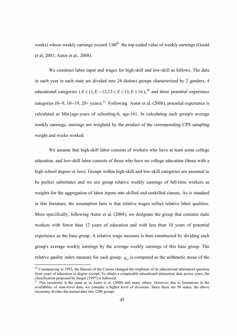
45

weeks) whose weekly earnings exceed 1/40th the top-coded value of weekly earnings (Gould

et al, 2001; Autor et al., 2008).

We construct labor input and wages for high-skill and low-skill as follows. The data

in each year in each state are divided into 24 distinct groups characterized by 2 genders, 4

educational categories ( 11, 12,13 15, 16E E E E≤ = ≤ ≤ ≥ ),20 and three potential experience

categories (0--9, 10--19, 20+ years).21 Following Autor et al. (2008), potential experience is

calculated as Min{age-years of schooling-6, age-16}. In calculating each group's average

weekly earnings, earnings are weighted by the product of the corresponding CPS sampling

weight and weeks worked.

We assume that high-skill labor consists of workers who have at least some college

education, and low-skill labor consists of those who have no college education (those with a

high school degree or less). Groups within high-skill and low-skill categories are assumed to

be perfect substitutes and we use group relative weekly earnings of full-time workers as

weights for the aggregation of labor inputs into skilled and unskilled classes. As is standard

in this literature, the assumption here is that relative wages reflect relative labor qualities.

More specifically, following Autor et al. (2008), we designate the group that contains male

workers with fewer than 12 years of education and with less than 10 years of potential

experience as the base group. A relative wage measure is then constructed by dividing each

group's average weekly earnings by the average weekly earnings of this base group. The

relative quality index measure for each group, ,gq is computed as the arithmetic mean of the 20 Commencing in 1992, the Bureau of the Census changed the emphasis of its educational attainment question from years of education to degree receipt. To obtain a comparable educational-attainment data across years, the classification proposed by Jaeger (1997) is followed. 21 This taxonomy is the same as in Autor et al. (2008) and many others. However, due to limitations in the availability of state-level data, we consider a higher level of divisions. Since there are 50 states, the above taxonomy divides the annual data into 1200 groups.

46

relative wage measures in that group over 1977 to 2009. Then the total quality-adjusted

labor input in each class is given by

, ,H L

t g gt t g gtg G g G

H q N L q N∈ ∈

= =∑ ∑

where gtN represents the total labor weeks in group g in year t.

Following Krusell et al. (2000), we calculate quality-adjusted earnings for skilled and

unskilled labor

, ,H L

g t g t g t g tH t L t

g G g Gt t

W N W NW W

H L∈ ∈

= =∑ ∑

where gtW represents the average weekly earnings of group g in year t.

As an alternative measure of earnings, we adjust for the composition of labor input so

that the average weekly earnings of high-skill and low-skill workers are not mechanically

affected by shifts in the experience, gender composition, or average level of completed

schooling (Autor et al. 2008). To this end, we first normalize the labor input in each group

by the total labor input in its class (i.e., ,j

gt gt gtg Gn N N

∈= ∑ j=H, L). The composition

index for each group, ,gn is computed as the arithmetic mean of gtn over 1977 to 2009. Then

the composition-adjusted weekly wages are

, .H L

Ht g gt Lt g gtg G g G

W n W W n W∈ ∈

= =∑ ∑

Calculation of adjusted earnings and labor as described above allows us to construct the

measures of relative efficiency as portrayed in Equation (5).

47

A.2. Industry-State Level Construction

Construction of the key variables at the industry level follows the same steps. In each state,

industries are classifies into three categories: service, manufacturing, and other (agriculture +

mining + construction). Annual data in each industry in each state are divided into 8 distinct

groups characterized by 2 gender and 4 education categories as in the state-level analysis.22

In calculating each group's average weekly earnings, earnings are weighted by the product of

the corresponding CPS sampling weight and weeks worked. High-skill and low-skill labor

classes are the same as above; and while aggregating labor inputs into skilled and unskilled

classes, we choose the group that contains male workers with less than 12 years of education

as the base group.

22 Unlike the state-level analysis, this partition does not include experience due to the limited number of observations.

48

References

Acemoglu, Daron, “Directed Technical Change,” Review of Economic Studies, October 2002, 69, 781-809.

Autor, David H., Lawrence F. Katz, and Melissa S. Kearney, “Trends in U.S. Wage In- equality: Revising the Revisionists,” Review of Economics and Statistics, May 2008, 90, 300-323.

Autor, David H., Lawrence F., Katz, Alan B., Krueger, “Computing Inequality: Have Computers Changed the Labor Market?” The Quarterly Journal of Economics, Vol. 113, No. 4 (Nov., 1998), pp. 1169-1213

Berry, William D., Richard C. Fording, and Russell L. Hanson, “An Annual Cost of Living Index for the American States, 1960-95,” Journal of Politics, 2000, 62, 550-67

Bound, John and George, Johnson, “Changes in the Structure of Wages in the 1980's: An Evaluation of Alternative Explanations,” The American Economic Review, Vol. 82, No. 3 (Jun., 1992), pp. 371-392

Card, David and John E., DiNardo, “Skill-Biased Technological Change and Rising Wage Inequality: Some Problems and Puzzles,” Journal of Labor Economics, 2002, vol. 20, No. 4; pp. 733-83.

Card, David, and Thomas Lemieux, “Can Falling Supply Explain the Rising Return to College for Younger Men?” Quarterly Journal of Economics 116 (May 2001), pp. 705-46

Caselli, Francesco and Willbur John Coleman II, “The World Technology Frontier,” American Economic Review, 2006, 96, pp. 499-522.

Ciccone, Antonio and Giovanni Peri, “Long-run Substitutability between More and Less Educa- ted Workers: Evidence from U.S. States 1950-90,” Review of Economics and Statistics, 2005, 87, pp. 652-63

Corman, Hope, and H. Naci Mocan, “A Time-Series Analysis of Crime, Deterrence, and Drug Abuse in New York City,” American Economic Review 90 (2000): 584-604.

Doms, Mark, Timothy Dunne, and Kenneth R. Troske, “Workers, Wages and Technology,” Quarterly Journal of Economics 122 (February 1997), 253-290

Ehrlich, Isaac, “Participation in Illegitimate Activities: A Theoretical and Empirical Investigation” The Journal of Political Economy, Vol. 81, No. 3 (May - Jun., 1973), pp. 521-565

Gould, Eric D., Bruce A. Weinberg, and David B. Mustard, “Crime Rates and Local Labor Market Opportunities in the United States: 1979-1997,” Review of Economics and Statistics, 2002, 84(1), 45-61.

49

Grogger, Jeff, “Market Wages and Youth Crime,” Journal of Labor Economics, Volume 16, Number 4, October 1998, pp.756-791

Juhn, Chinhui, Kevin M. Murphy, and Brooks Pierce, “Wage Inequality and the Rise in Returns to Skill,” Journal of Political Economy 101 (June 1993), 410-442.

Katz, Lawrence F. and David H., Autor, 1999, “Changes in the Wage Structure and Earnings Inequality,” in: O. Ashenfelter and D. Card (ed.), Handbook of Labor Economics, ed. 1,Volume 3, Chapter 26, p. 1463-1555 Elsevier

Katz, Lawrence F. and Kevin M. Murphy, “Changes in Relative Wages, 1963-87: Supply and Demand Factors,” Quarterly Journal of Economics, 1992, 107, 35-78.

Katz, Lawrence F., Steven D. Levitt,and Ellen Shustorovich, “Prison Conditions, Capital Punishment and Deterrence,” American Law and Economics Review 5 (2003): 318- 43.

Krusell, Per, Lee E. Ohanian, Jose-Victor Rios-Rull, and Giovanni L. Violante, “Capital Skill Complementarity and Inequality: A Macroeconomic Analysis,” Econometrica, 2000, 68, 1029-53. Lemieux, Thomas, “Increasing Residual Wage Inequality: Composition Effects, Noisy Data, or Rising Demand for Skill?” The American Economic Review, Vol. 96, No. 3 (Jun., 2006), pp. 461-498

Levitt, Stephen D., “Juvenile Crime and Punishment,” Journal of Political Economy 106 (1998): 1156-85

Machin, Stephen and Costas Meghir, “Crime and Economic Incentives,” Journal of Human Resources (2004) 39:4, 958-79.

Mocan, H. Naci, Billups, Stephen C., and Overland, Jody, “A Dynamic Model of Differential Human Capital and Criminal Activity,” Economica (2005) 72, 655–681

Mocan, H. Naci, Turan G. Bali, “Asymmetric Crime Cycles” The Review of Economics and Statistics, Vol.XCII, November 2010, Number 4, 899-911

Skill-biased Technological Change, Earnings of Unskilled … · 2018-10-29 · 1 Skill-biased...

Documents

Transcript of Skill-biased Technological Change, Earnings of Unskilled … · 2018-10-29 · 1 Skill-biased...