Skeletons CSE169: Computer Animation Instructor: Steve Rotenberg UCSD, Winter 2005.
164
Skeletons CSE169: Computer Animation Instructor: Steve Rotenberg UCSD, Winter 2005
-
Upload
nickolas-potter -
Category
Documents
-
view
221 -
download
0
Transcript of Skeletons CSE169: Computer Animation Instructor: Steve Rotenberg UCSD, Winter 2005.
Skeletons
CSE169: Computer Animation
Instructor: Steve Rotenberg
UCSD, Winter 2005
Kinematics
Kinematics: The analysis of motion independent of physical forces. Kinematics deals with position, velocity, acceleration, and their rotational counterparts, orientation, angular velocity, and angular acceleration.
Forward Kinematics: The process of computing world space geometric data from DOFs
Inverse Kinematics: The process of computing a set of DOFs that causes some world space goal to be met (I.e., place the hand on the door knob…)
Note: Kinematics is an entire branch of mathematics and there are several other aspects of kinematics that don’t fall into the ‘forward’ or ‘inverse’ description

Skeletons
Skeleton: A pose-able framework of joints arranged in a tree structure. The skeleton is used as an invisible armature to manipulate the skin and other geometric data of the character
Joint: A joint allows relative movement within the skeleton. Joints are essentially 4x4 matrix transformations. Joints can be rotational, translational, or some non-realistic types as well
Bone: Bone is really just a synonym for joint for the most part. For example, one might refer to the shoulder joint or upper arm bone (humerus) and mean the same thing
DOFs
Degree of Freedom (DOF): A variable φ describing a particular axis or dimension of movement within a joint
Joints typically have around 1-6 DOFs (φ1…φN) Changing the DOF values over time results in
the animation of the skeleton In later weeks, we will extend the concept of a
DOF to be any animatable parameter within the character rig
Note: in a mathematical sense, a free rigid body has 6 DOFs: 3 for position and 3 for rotation
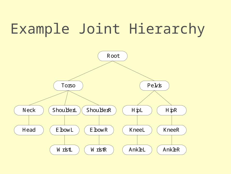
Example Joint Hierarchy
Root
Torso
Neck
Pelvis
HipL HipR
Head ElbowL
WristL
ElbowR
WristR
KneeL
AnkleL
KneeR
AnkleR
ShoulderL ShoulderR
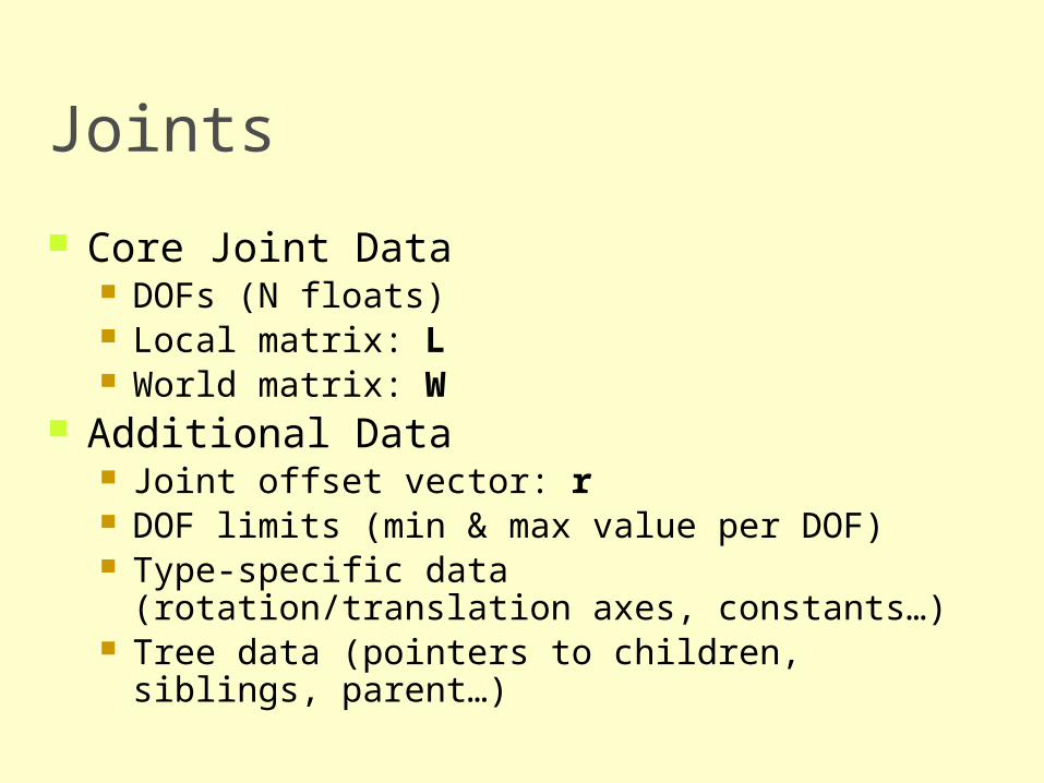
Joints
Core Joint Data DOFs (N floats) Local matrix: L World matrix: W
Additional Data Joint offset vector: r DOF limits (min & max value per DOF) Type-specific data (rotation/translation axes,
constants…) Tree data (pointers to children, siblings, parent…)
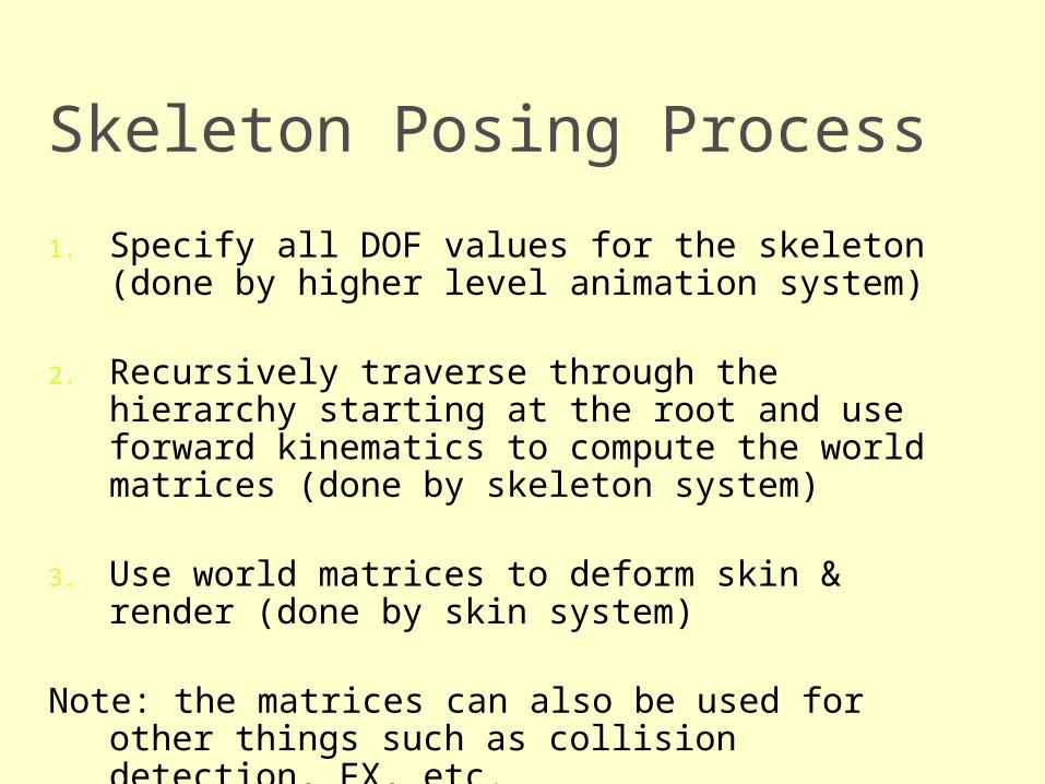
Skeleton Posing Process
1. Specify all DOF values for the skeleton (done by higher level animation system)
2. Recursively traverse through the hierarchy starting at the root and use forward kinematics to compute the world matrices (done by skeleton system)
3. Use world matrices to deform skin & render (done by skin system)
Note: the matrices can also be used for other things such as collision detection, FX, etc.
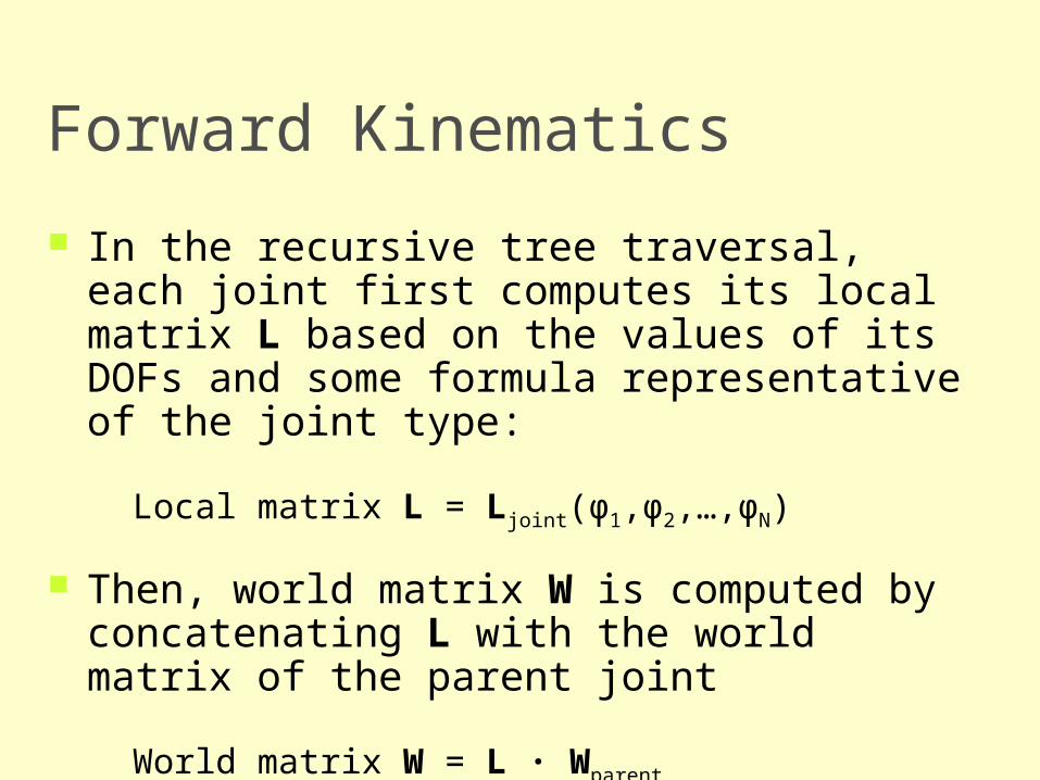
Forward Kinematics
In the recursive tree traversal, each joint first computes its local matrix L based on the values of its DOFs and some formula representative of the joint type:
Local matrix L = Ljoint(φ1,φ2,…,φN)
Then, world matrix W is computed by concatenating L with the world matrix of the parent joint
World matrix W = L · Wparent
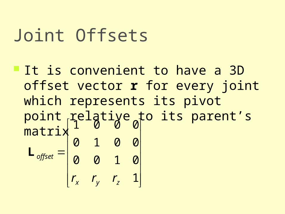
Joint Offsets
It is convenient to have a 3D offset vector r for every joint which represents its pivot point relative to its parent’s matrix
1
0100
0010
0001
zyx
offset
rrr
L
DOF Limits
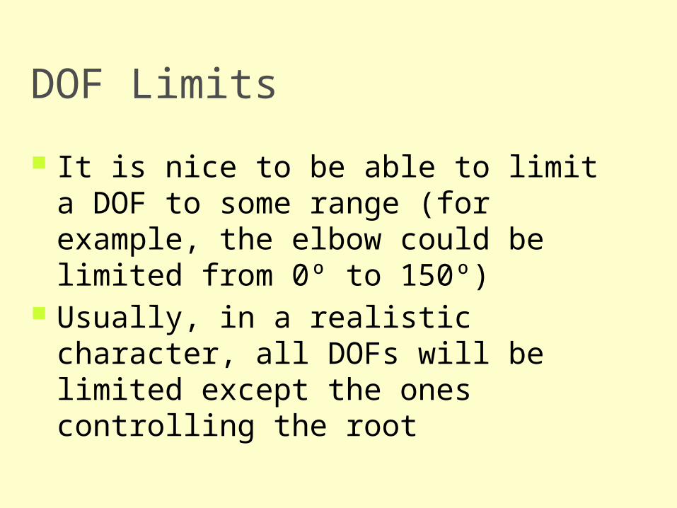
It is nice to be able to limit a DOF to some range (for example, the elbow could be limited from 0º to 150º)
Usually, in a realistic character, all DOFs will be limited except the ones controlling the root
Skeleton Rigging
Setting up the skeleton is an important and early part of the rigging process
Sometimes, character skeletons are built before the skin, while other times, it is the opposite
To set up a skeleton, an artist uses an interactive tool to: Construct the tree Place joint offsets Configure joint types Specify joint limits Possibly more…
Poses
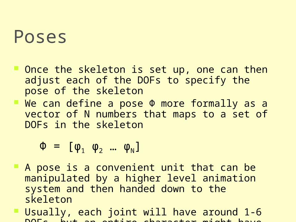
Once the skeleton is set up, one can then adjust each of the DOFs to specify the pose of the skeleton
We can define a pose Φ more formally as a vector of N numbers that maps to a set of DOFs in the skeleton
Φ = [φ1 φ2 … φN]
A pose is a convenient unit that can be manipulated by a higher level animation system and then handed down to the skeleton
Usually, each joint will have around 1-6 DOFs, but an entire character might have 100+ DOFs in the skeleton
Keep in mind that DOFs can be also used for things other than joints, as we will learn later…
Joint Types
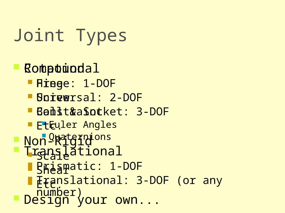
Joint Types
Rotational Hinge: 1-DOF Universal: 2-DOF Ball & Socket: 3-DOF
Euler Angles Quaternions
Translational Prismatic: 1-DOF Translational: 3-DOF (or any number)
Compound Free Screw Constraint Etc.
Non-Rigid Scale Shear Etc.
Design your own...
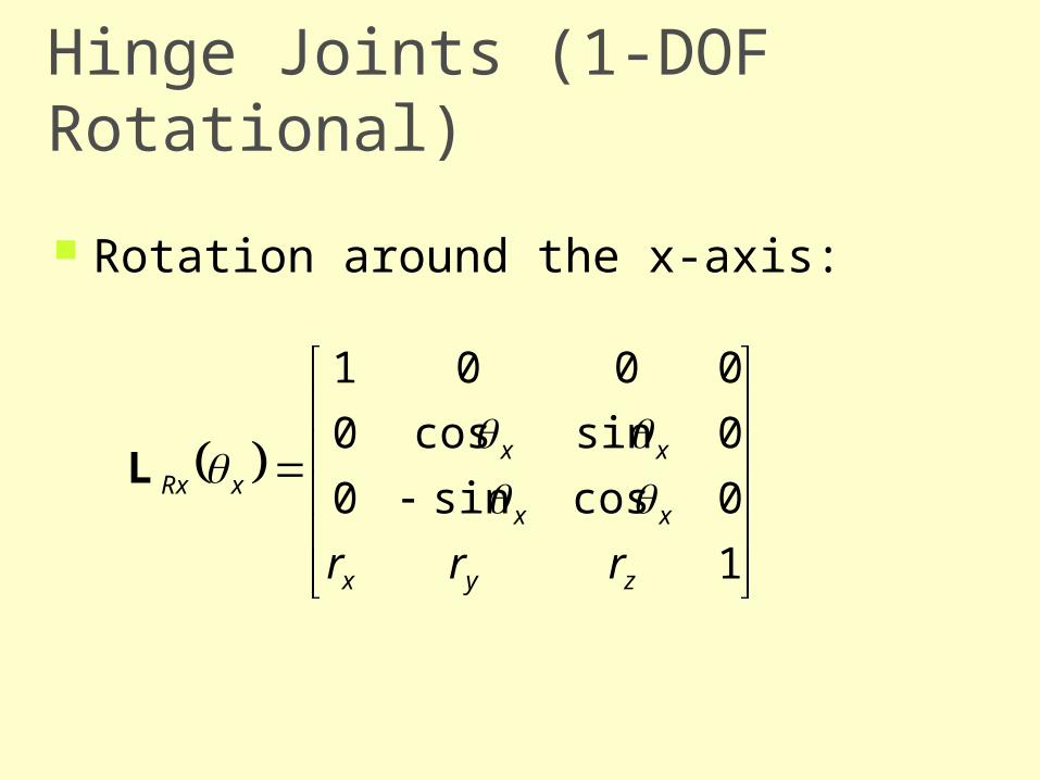
Hinge Joints (1-DOF Rotational)
1
0cossin0
0sincos0
0001
zyx
xx
xxxRx
rrr
L
Rotation around the x-axis:
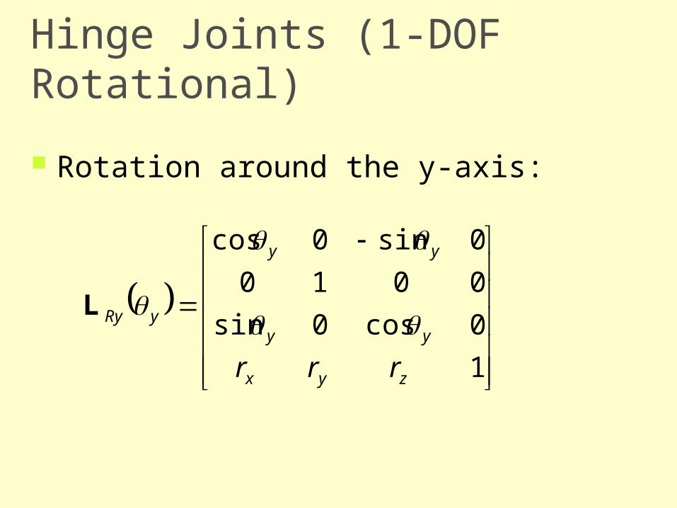
Hinge Joints (1-DOF Rotational)
1
0cos0sin
0010
0sin0cos
zyx
yy
yy
yRy
rrr
L
Rotation around the y-axis:
Hinge Joints (1-DOF Rotational)
1
0100
00cossin
00sincos
zyx
zz
zz
zRz
rrr
L
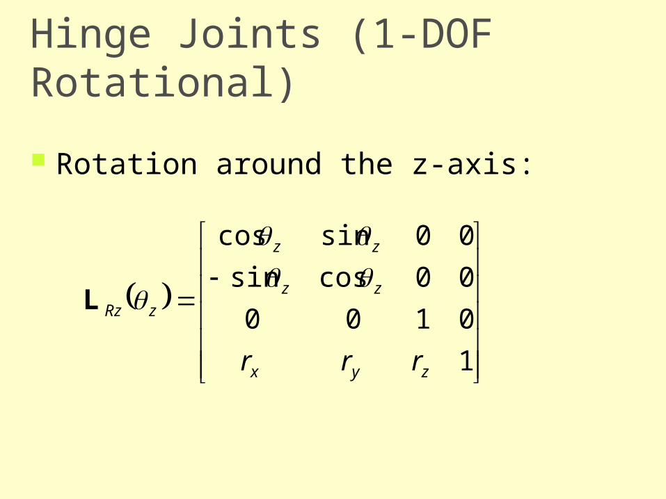
Rotation around the z-axis:
Hinge Joints (1-DOF Rotational)
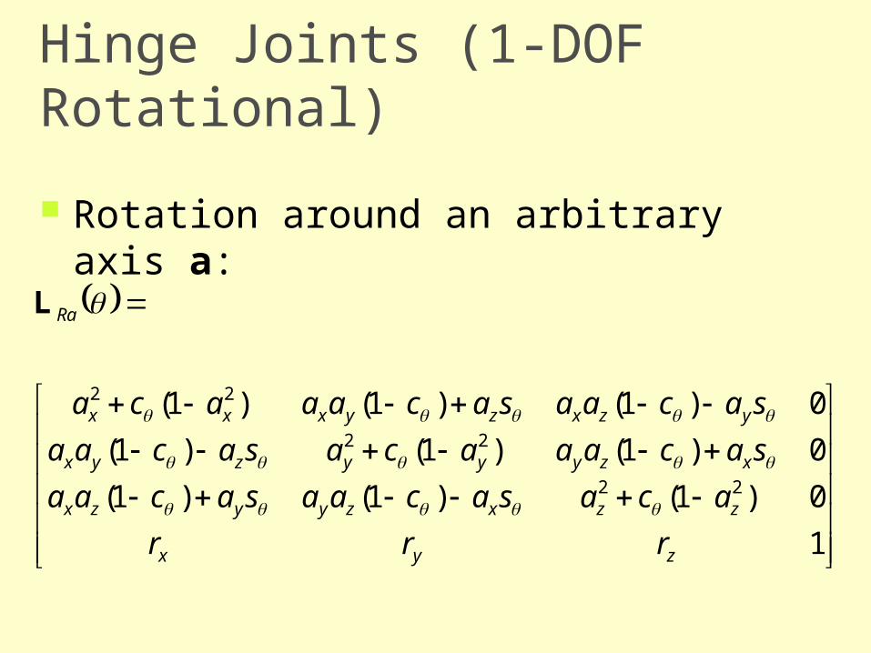
Rotation around an arbitrary axis a:
1
0)1()1()1(
0)1()1()1(
0)1()1()1(
22
22
22
zyx
zzxzyyzx
xzyyyzyx
yzxzyxxx
Ra
rrr
acasacaasacaa
sacaaacasacaa
sacaasacaaaca
L
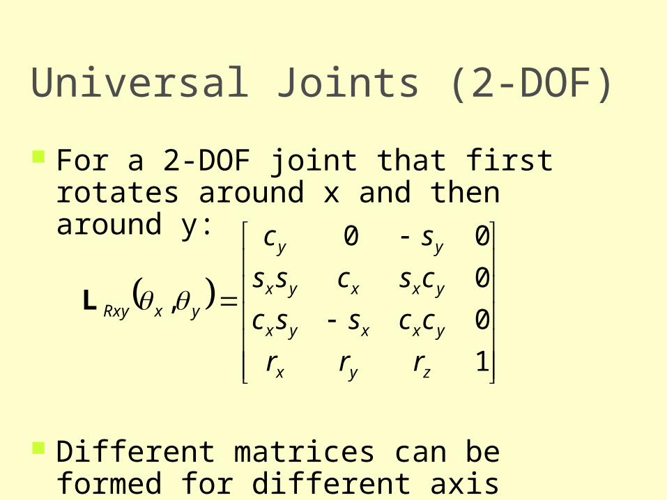
Universal Joints (2-DOF)
For a 2-DOF joint that first rotates around x and then around y:
Different matrices can be formed for different axis combinations
1
0
0
00
,
zyx
yxxyx
yxxyx
yy
yxRxy
rrr
ccssc
cscss
sc
L
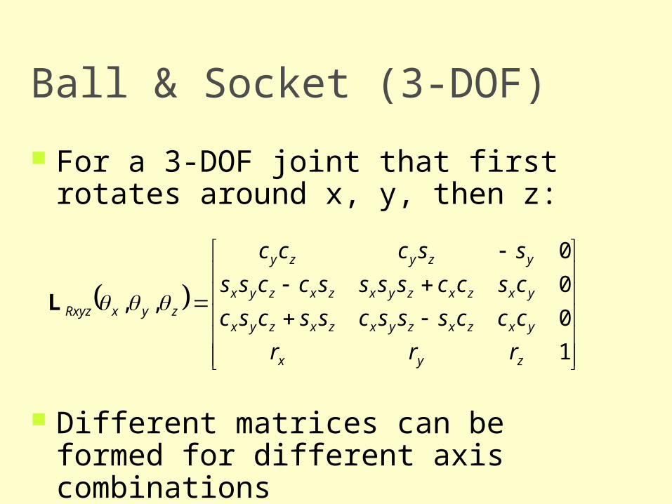
Ball & Socket (3-DOF)
For a 3-DOF joint that first rotates around x, y, then z:
Different matrices can be formed for different axis combinations
1
0
0
0
,,
zyx
yxzxzyxzxzyx
yxzxzyxzxzyx
yzyzy
zyxRxyz
rrr
cccssscsscsc
csccssssccss
ssccc
L
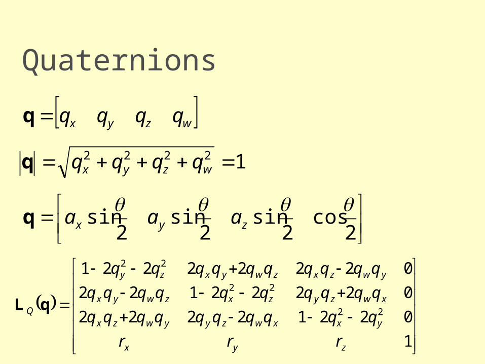
Quaternions
wzyx qqqqq
12222 wzyx qqqqq
2cos
2sin
2sin
2sin
zyx aaaq
1
02212222
02222122
02222221
22
22
22
zyx
yxxwzyywzx
xwzyzxzwyx
ywzxzwyxzy
Q
rrr
qqqqqqqqqq
qqqqqqqqqq
qqqqqqqqqq
qL
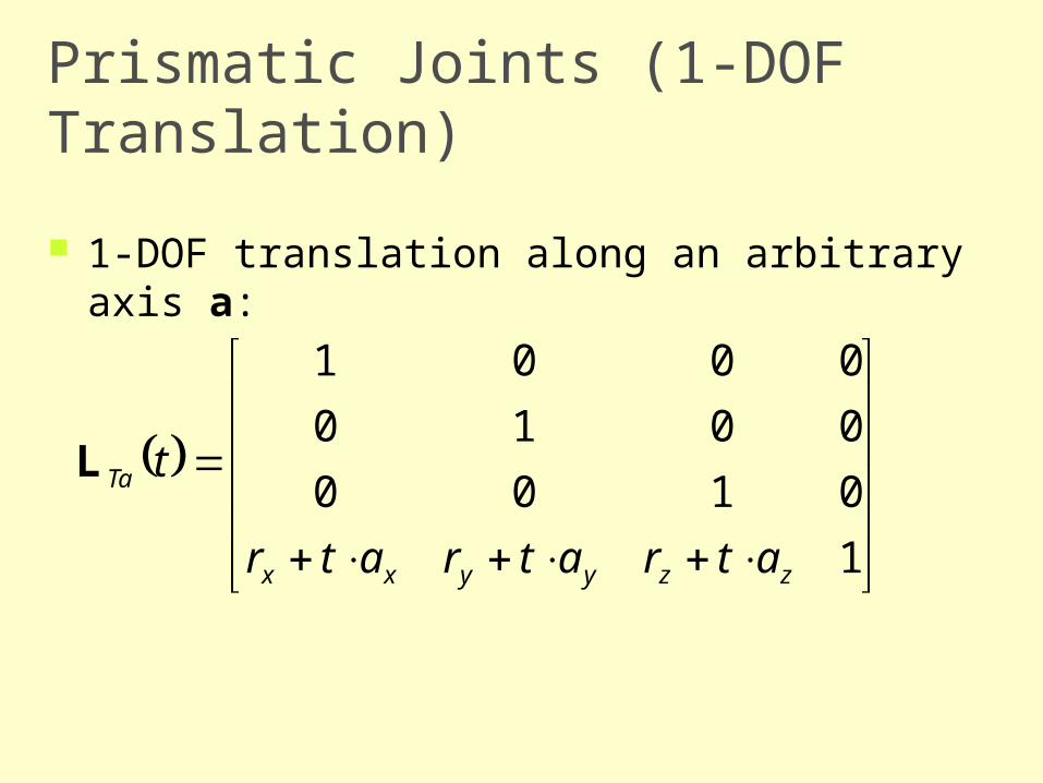
Prismatic Joints (1-DOF Translation)
1-DOF translation along an arbitrary axis a:
1
0100
0010
0001
zzyyxx
Ta
atratratr
tL
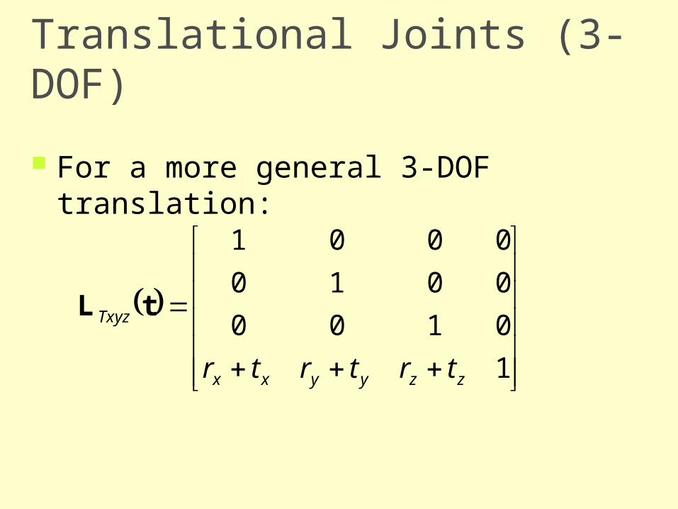
Translational Joints (3-DOF)
For a more general 3-DOF translation:
1
0100
0010
0001
zzyyxx
Txyz
trtrtr
tL
Other Joints
Compound Free Screw Constraint Etc.
Non-Rigid Scale (1 axis, 3 axis, volume preserving…) Shear Etc.
Skin
CSE169: Computer Animation
Instructor: Steve Rotenberg
UCSD, Winter 2005
Texture
We may wish to ‘map’ various properties across the polygonal surface
We can do this through texture mapping, or other more general mapping techniques
Usually, this will require explicitly storing texture coordinate information at the vertices
For higher quality rendering, we may combine several different maps in complex ways, each with their own mapping coordinates
Related features include bump mapping, displacement mapping, illumination mapping…
Smooth Skin Algorithm
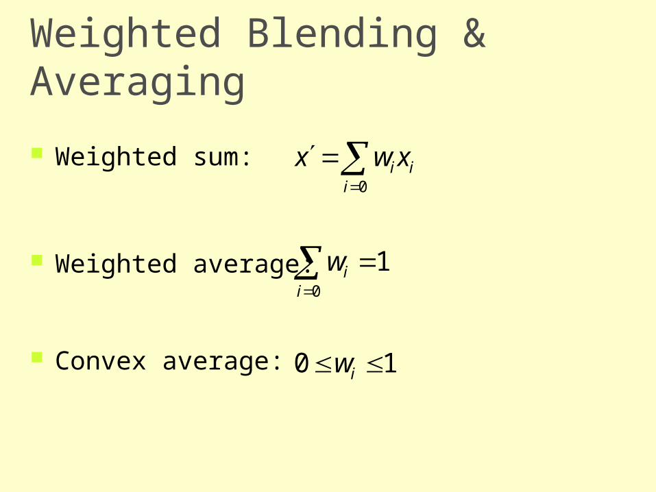
Weighted Blending & Averaging
Weighted sum:
Weighted average:
Convex average: 10
10
0
i
ii
iii
w
w
xwx
Rigid Parts
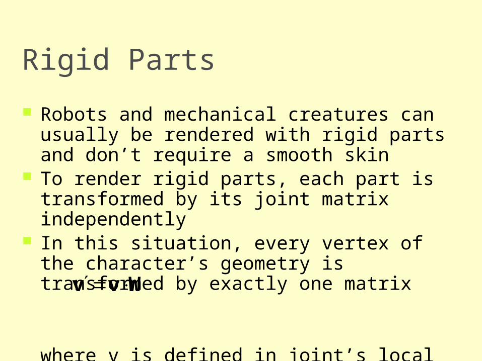
Robots and mechanical creatures can usually be rendered with rigid parts and don’t require a smooth skin
To render rigid parts, each part is transformed by its joint matrix independently
In this situation, every vertex of the character’s geometry is transformed by exactly one matrix
where v is defined in joint’s local space
Wvv
Simple Skin
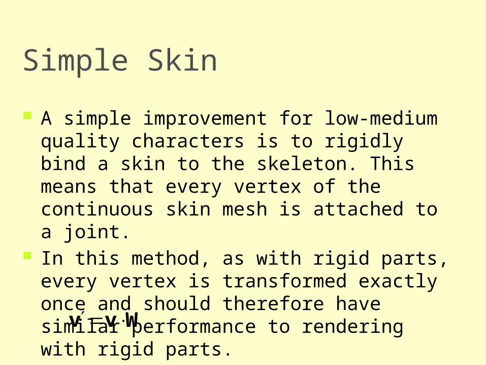
A simple improvement for low-medium quality characters is to rigidly bind a skin to the skeleton. This means that every vertex of the continuous skin mesh is attached to a joint.
In this method, as with rigid parts, every vertex is transformed exactly once and should therefore have similar performance to rendering with rigid parts.
Wvv
Smooth Skin
With the smooth skin algorithm, a vertex can be attached to more than one joint with adjustable weights that control how much each joint affects it
Verts rarely need to be attached to more than three joints
Each vertex is transformed a few times and the results are blended
The smooth skin algorithm has many other names: blended skin, skeletal subspace deformation (SSD), multi-matrix skin, matrix palette skinning…
Smooth Skin Algorithm
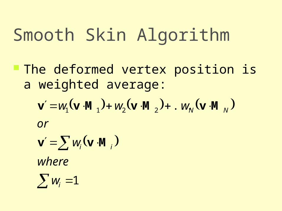
The deformed vertex position is a weighted average:
1
...2211
i
ii
NN
w
where
w
or
www
Mvv
MvMvMvv
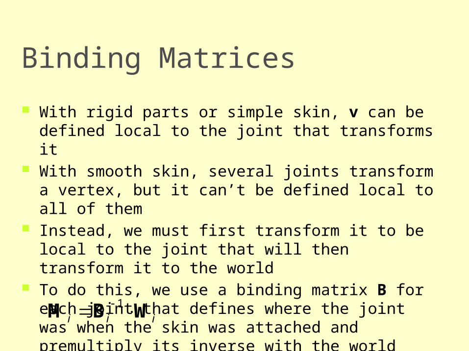
Binding Matrices
With rigid parts or simple skin, v can be defined local to the joint that transforms it
With smooth skin, several joints transform a vertex, but it can’t be defined local to all of them
Instead, we must first transform it to be local to the joint that will then transform it to the world
To do this, we use a binding matrix B for each joint that defines where the joint was when the skin was attached and premultiply its inverse with the world matrix:
iii WBM 1
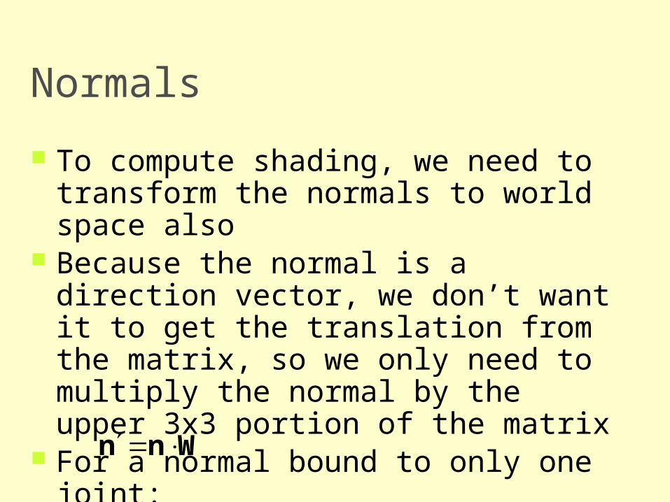
Normals
To compute shading, we need to transform the normals to world space also
Because the normal is a direction vector, we don’t want it to get the translation from the matrix, so we only need to multiply the normal by the upper 3x3 portion of the matrix
For a normal bound to only one joint:
Wnn
Normals
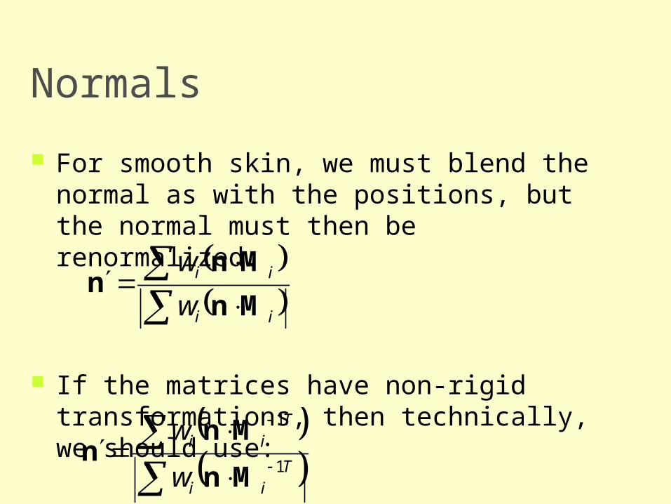
For smooth skin, we must blend the normal as with the positions, but the normal must then be renormalized:
If the matrices have non-rigid transformations, then technically, we should use:
ii
ii
w
w
Mn
Mnn
Tii
Tii
w
w1
1
Mn
Mnn
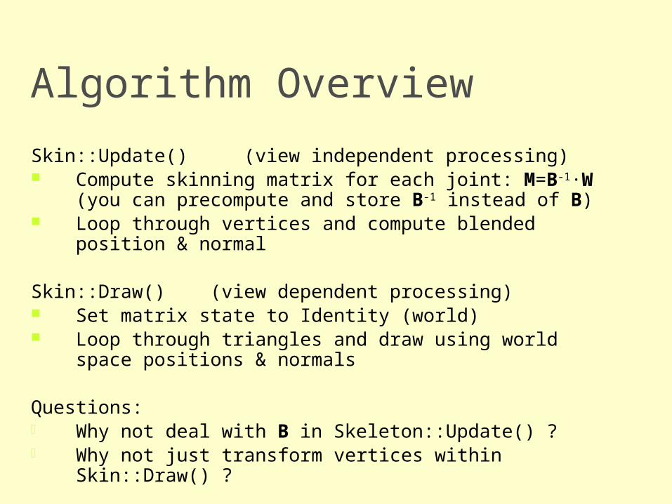
Algorithm Overview
Skin::Update() (view independent processing) Compute skinning matrix for each joint: M=B-1·W (you can
precompute and store B-1 instead of B) Loop through vertices and compute blended position & normal
Skin::Draw() (view dependent processing) Set matrix state to Identity (world) Loop through triangles and draw using world space positions &
normals
Questions:- Why not deal with B in Skeleton::Update() ?- Why not just transform vertices within Skin::Draw() ?
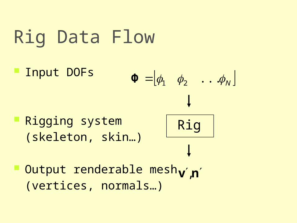
Rig Data Flow
Input DOFs
Rigging system
(skeleton, skin…)
Output renderable mesh
(vertices, normals…)
N ...21Φ
nv ,
Rig
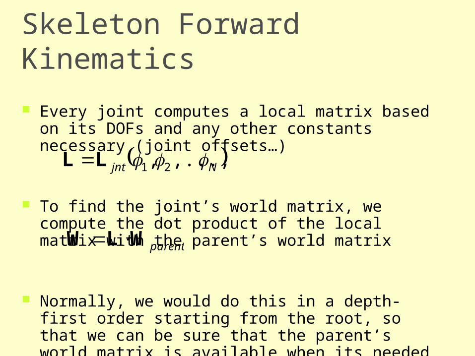
Skeleton Forward Kinematics
Every joint computes a local matrix based on its DOFs and any other constants necessary (joint offsets…)
To find the joint’s world matrix, we compute the dot product of the local matrix with the parent’s world matrix
Normally, we would do this in a depth-first order starting from the root, so that we can be sure that the parent’s world matrix is available when its needed
Njnt ,...,, 21LL
parentWLW
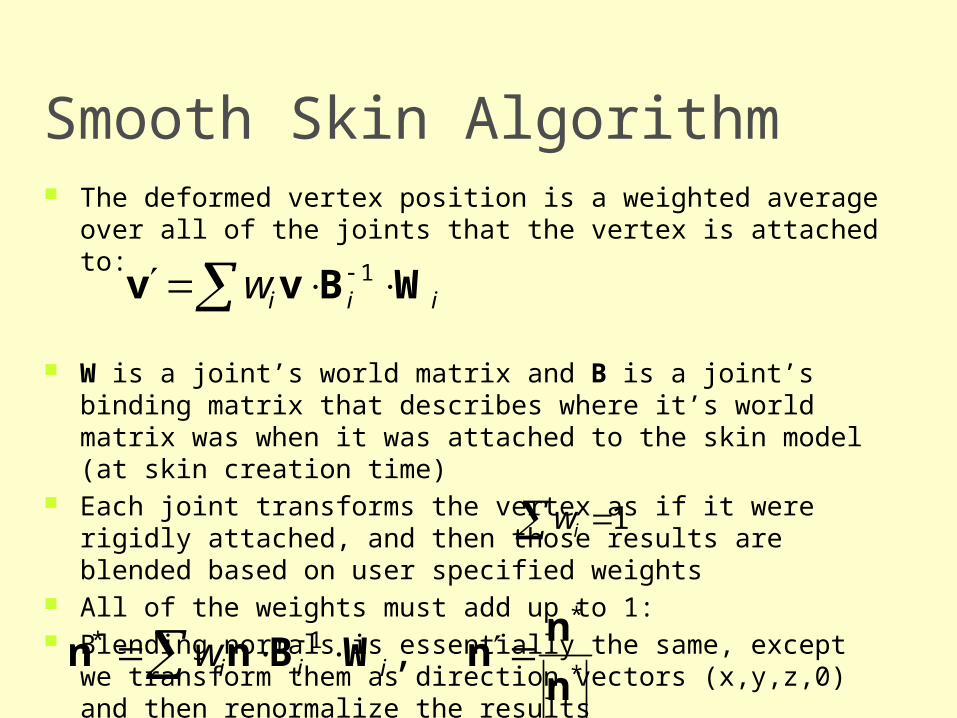
Smooth Skin Algorithm The deformed vertex position is a weighted average over all of the
joints that the vertex is attached to:
W is a joint’s world matrix and B is a joint’s binding matrix that describes where it’s world matrix was when it was attached to the skin model (at skin creation time)
Each joint transforms the vertex as if it were rigidly attached, and then those results are blended based on user specified weights
All of the weights must add up to 1: Blending normals is essentially the same, except we transform them
as direction vectors (x,y,z,0) and then renormalize the results
iiiw WBvv 1
1iw
*
*1* ,
n
nnWBnn
iiiw
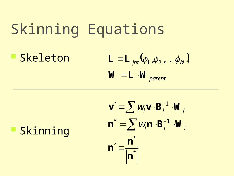
Skinning Equations
*
*
1*
1
21 ,...,,
n
nn
WBnn
WBvv
WLW
LL
iii
iii
parent
Njnt
w
w
Skeleton
Skinning
Using Skinning
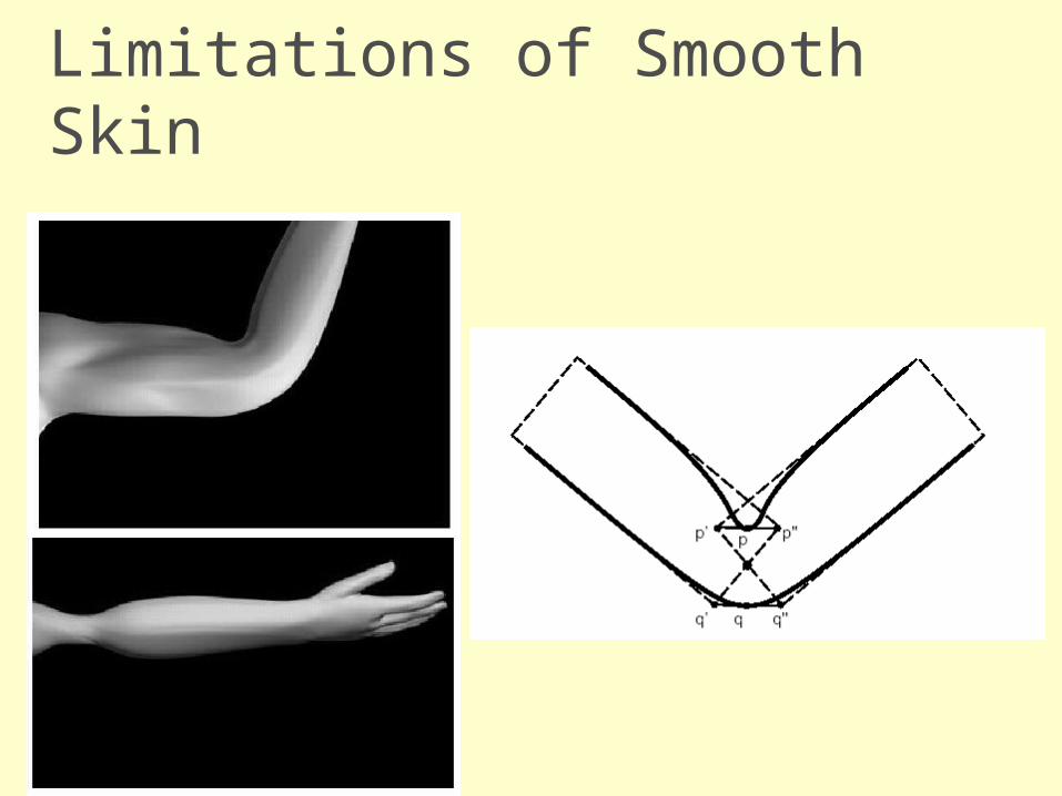
Limitations of Smooth Skin
Smooth skin is very simple and quite fast, but its quality is limited
The main problems are: Joints tend to collapse as they bend more Very difficult to get specific control Unintuitive and difficult to edit
Still, it is built in to most 3D animation packages and has support in both OpenGL and Direct3D
If nothing else, it is a good baseline upon which more complex schemes can be built
Limitations of Smooth Skin
Bone Links
To help with the collapsing joint problem, one option is to use bone links
Bone links are extra joints inserted in the skeleton to assist with the skinning
They can be automatically added based on the joint’s range of motion. For example, they could be added so as to prevent any joint from rotating more than 60 degrees.
This is a simple approach used in some real time games, but doesn’t go very far in fixing the other problems with smooth skin.
Shape Interpolation
Another extension to the smooth skinning algorithm is to allow the verts to be modeled at key values along the joints motion
For an elbow, for example, one could model it straight, then model it fully bent
These shapes are interpolated local to the bones before the skinning is applied
We will talk more about this technique in the next lecture
Muscles & Other Effects
One can add custom effects such as muscle bulges as additional joints
For example, the bicep could be a translational or scaling joint that smoothly controls some of the verts in the upper arm. Its motion could be linked to the motion of the elbow rotation.
With this approach, one can also use skin for muscles, fat bulges, facial expressions, and even simple clothing
We will learn more about advanced skinning techniques in a later lecture
Rigging Process
To rig a skinned character, one must have a geometric skin mesh and a skeleton
Usually, the skin is built in a relatively neutral pose, often in a comfortable standing pose
The skeleton, however, might be built in more of a zero pose where the joints DOFs are assumed to be 0, causing a very stiff, straight pose
To attach the skin to the skeleton, the skeleton must first be posed into a binding pose
Once this is done, the verts can be assigned to joints with appropriate weights
Skin Binding
Attaching a skin to a skeleton is not a trivial problem and usually requires automated tools combined with extensive interactive tuning
Binding algorithms typically involve heuristic approaches
Some general approaches: Containment Point-to-line mapping Delaunay tetrahedralization
Containment Binding
With containment binding algorithms, the user manually approximates the body with volume primitives for each bone (cylinders, ellipsoids, spheres…)
The algorithm then tests each vertex against the volumes and attaches it to the best fitting bone
Some containment algorithms attach to only one bone and then use smoothing as a second pass. Others attach to multiple bones directly and set skin weights
For a more automated version, the volumes could be initially set based on the bone lengths and child locations
Point-to-Line Mapping
A simple way to attach a skin is treat each bone as one or more line segments and attach each vertex to the nearest line segment
A bone is made from line segments connecting the joint pivot to the pivots of each child

Delaunay Tetrahedralization
This tricky computational geometry technique builds a tetrahedralization of the volume within the skin
The tetrahedra connect all of the skin verts and skeletal pivots in a relatively clean ‘Delaunay’ fashion
The connectivity of the mesh can then be analyzed to determine the best attachment for each vertex
Skin Adjustment
Mesh Smoothing: A joint will first be attached in a fairly rigid fashion (either automatic or manually) and then the weights are smoothed algorithmically
Rogue Removal: Automatic identification and removal of isolated vertex attachments
Weight Painting: Some 3D tools allow visualization of the weights as colors (0…1 -> black…white). These can then be adjusted and ‘painted’ in an interactive fashion
Direct Manipulation: These algorithms allow the vertex to be moved to a ‘correct’ position after the bone is bent, and automatically compute the weights necessary to get it there
Hardware Skinning
The smooth skinning algorithm is simple and popular enough to have some direct support in 3D rendering hardware
Actually, it just requires standard vector multiply/add operations and so can be implemented in microcode
Skin Memory Usage For each vertex, we need to store:
Rendering data (position, normal, color, texture coords, tangents…)
Skinning data (number of attachments, joint index, weight…) If we limit the character to having at most 256 bones, we
can store a bone index as a byte If we limit the weights to 256 distinct values, we can
store a weight as a byte (this gives us a precision of 0.004%, which is fine)
If we assume that a vertex will attach to at most 4 bones, then we can compress the skinning data to (1+1)*4 =8 bytes per vertex (64 bits)
In fact, we can even squeeze another 8 bits out of that by not storing the final weight, since
w3 = 1 – w0 – w1 – w2
Inverse Kinematics (part 1)
CSE169: Computer Animation
Instructor: Steve Rotenberg
UCSD, Winter 2005
Welman, 1993
“Inverse Kinematics and Geometric Constraints for Articulated Figure Manipulation”, Chris Welman, 1993
Masters thesis on IK algorithms Examines Jacobian methods and Cyclic
Coordinate Descent (CCD) Please read sections 1-4 (about 40 pages)
Forward Kinematics
The local and world matrix construction within the skeleton is an implementation of forward kinematics
Forward kinematics refers to the process of computing world space geometric descriptions (matrices…) based on joint DOF values (usually rotation angles and/or translations)
Kinematic Chains
For today, we will limit our study to linear kinematic chains, rather than the more general hierarchies (i.e., stick with individual arms & legs rather than an entire body with multiple branching chains)
End Effector
The joint at the root of the chain is sometimes called the base
The joint (bone) at the leaf end of the chain is called the end effector
Sometimes, we will refer to the end effector as being a bone with position and orientation, while other times, we might just consider a point on the tip of the bone and only think about it’s position
Forward Kinematics
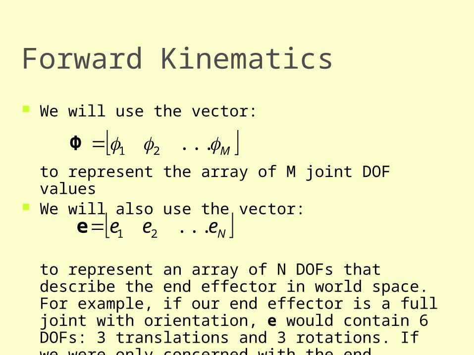
We will use the vector:
to represent the array of M joint DOF values We will also use the vector:
to represent an array of N DOFs that describe the end effector in world space. For example, if our end effector is a full joint with orientation, e would contain 6 DOFs: 3 translations and 3 rotations. If we were only concerned with the end effector position, e would just contain the 3 translations.
M ...21Φ
Neee ...21e
Forward Kinematics
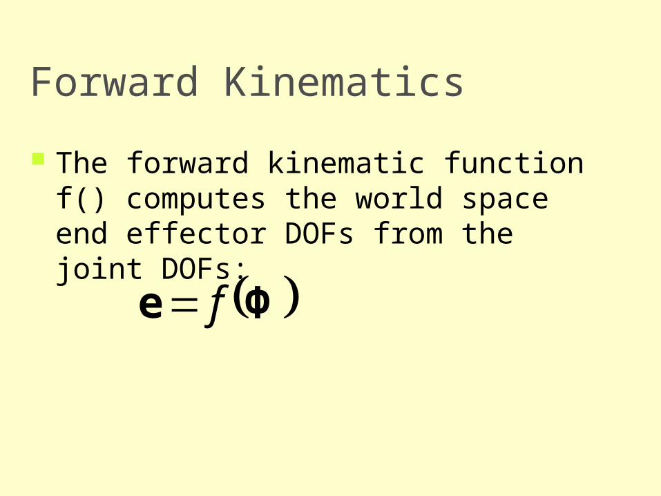
The forward kinematic function f() computes the world space end effector DOFs from the joint DOFs:
Φe f
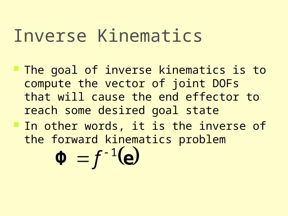
Inverse Kinematics
The goal of inverse kinematics is to compute the vector of joint DOFs that will cause the end effector to reach some desired goal state
In other words, it is the inverse of the forward kinematics problem
eΦ 1 f
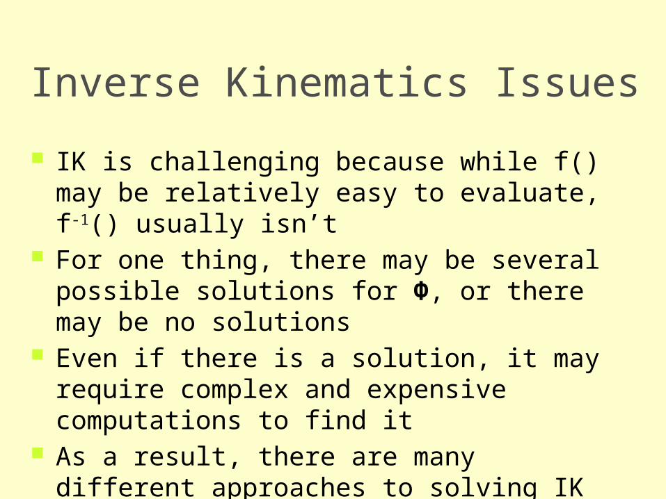
Inverse Kinematics Issues
IK is challenging because while f() may be relatively easy to evaluate, f-1() usually isn’t
For one thing, there may be several possible solutions for Φ, or there may be no solutions
Even if there is a solution, it may require complex and expensive computations to find it
As a result, there are many different approaches to solving IK problems
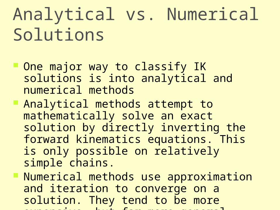
Analytical vs. Numerical Solutions
One major way to classify IK solutions is into analytical and numerical methods
Analytical methods attempt to mathematically solve an exact solution by directly inverting the forward kinematics equations. This is only possible on relatively simple chains.
Numerical methods use approximation and iteration to converge on a solution. They tend to be more expensive, but far more general purpose.
Today, we will examine a numerical IK technique based on Jacobian matrices

Calculus Review
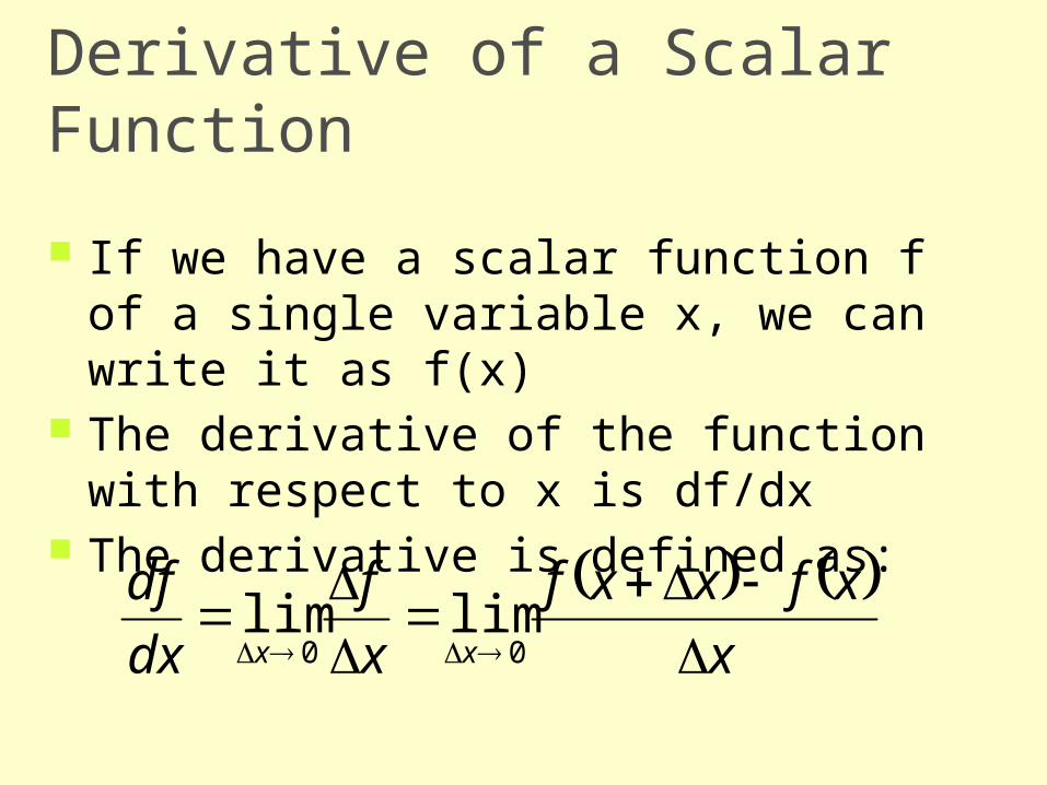
Derivative of a Scalar Function
If we have a scalar function f of a single variable x, we can write it as f(x)
The derivative of the function with respect to x is df/dx
The derivative is defined as:
x
xfxxf
x
f
dx
dfxx
00
limlim
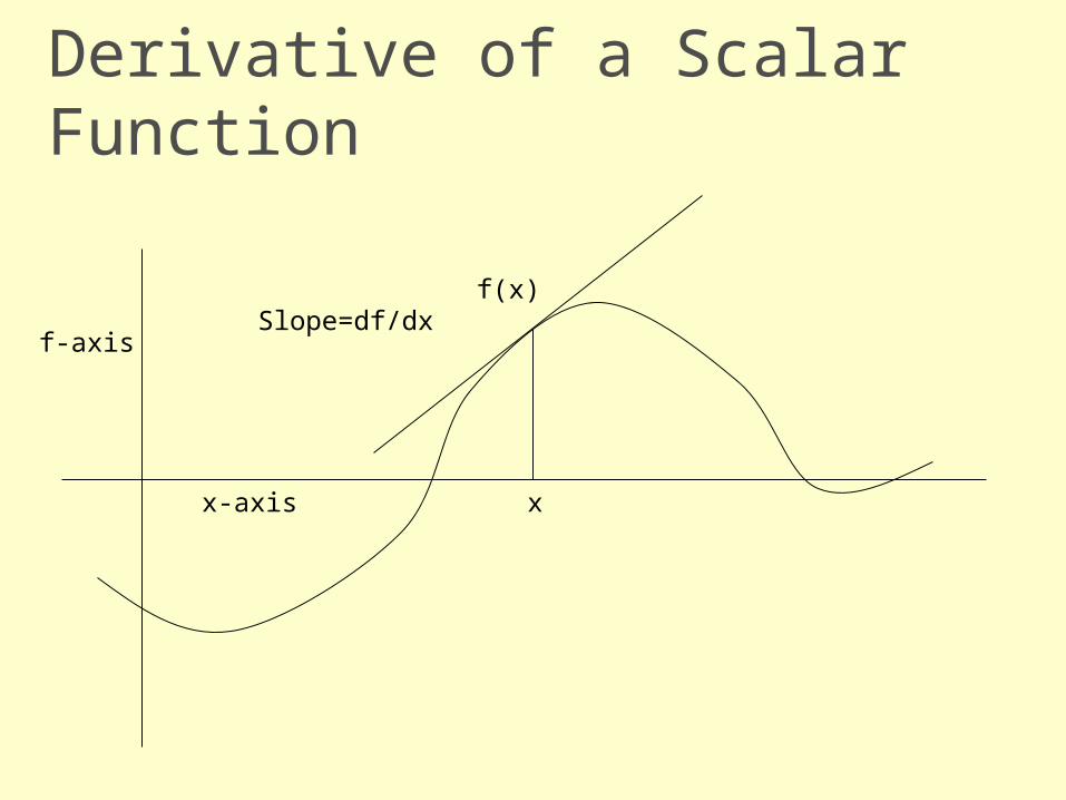
Derivative of a Scalar Function
f-axis
x-axis x
f(x)Slope=df/dx
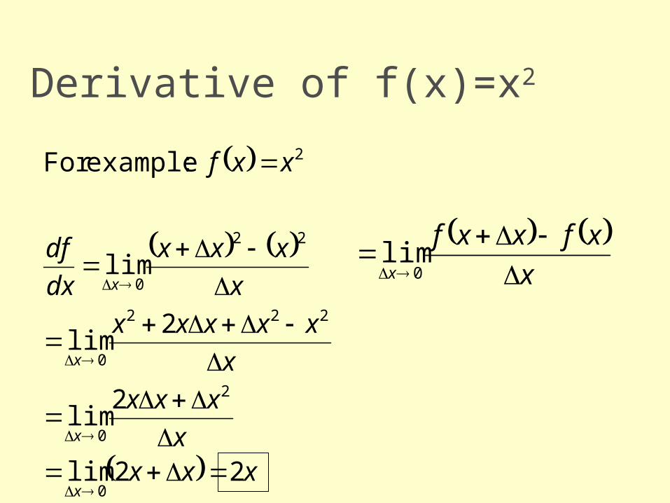
Derivative of f(x)=x2
xxxx
xxx
x
xxxxx
x
xxx
dx
df
xxf
x
x
x
x
22lim
2lim
2lim
lim
:exampleFor
0
2
0
222
0
22
0
2
x
xfxxfx
0lim
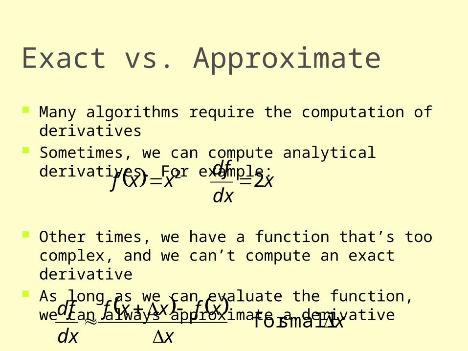
Exact vs. Approximate
Many algorithms require the computation of derivatives Sometimes, we can compute analytical derivatives. For
example:
Other times, we have a function that’s too complex, and we can’t compute an exact derivative
As long as we can evaluate the function, we can always approximate a derivative
xdx
dfxxf 2 2
x
x
xfxxf
dx
df
smallfor
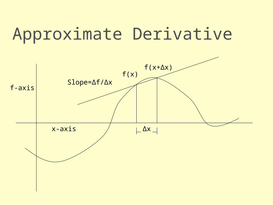
Approximate Derivative
f-axis
x-axis Δx
f(x)f(x+Δx)
Slope=Δf/Δx
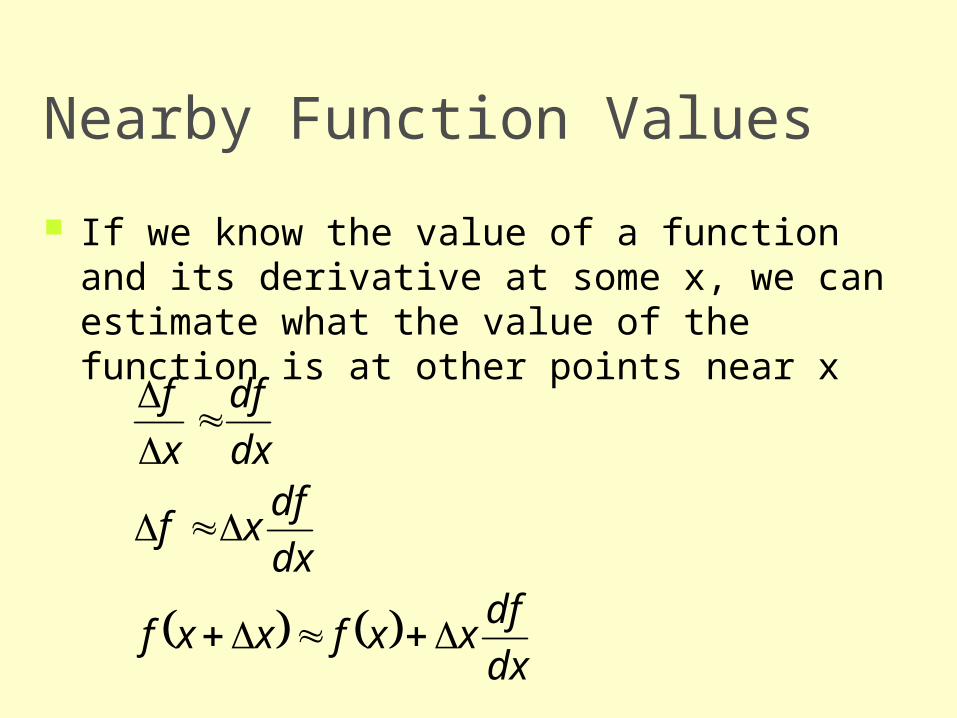
Nearby Function Values
If we know the value of a function and its derivative at some x, we can estimate what the value of the function is at other points near x
dx
dfxxfxxf
dx
dfxf
dx
df
x
f
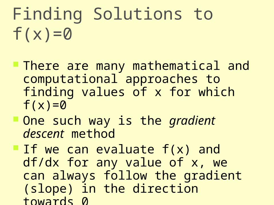
Finding Solutions to f(x)=0
There are many mathematical and computational approaches to finding values of x for which f(x)=0
One such way is the gradient descent method
If we can evaluate f(x) and df/dx for any value of x, we can always follow the gradient (slope) in the direction towards 0
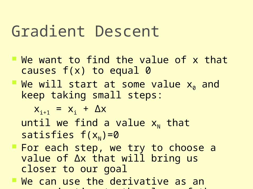
Gradient Descent
We want to find the value of x that causes f(x) to equal 0
We will start at some value x0 and keep taking small steps:
xi+1 = xi + Δx
until we find a value xN that satisfies f(xN)=0 For each step, we try to choose a value of Δx
that will bring us closer to our goal We can use the derivative as an approximation
to the slope of the function and use this information to move ‘downhill’ towards zero
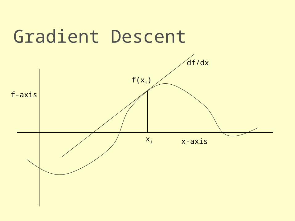
Gradient Descent
f-axis
x-axisxi
f(xi)
df/dx
Minimization
If f(xi) is not 0, the value of f(xi) can be thought of as an error. The goal of gradient descent is to minimize this error, and so we can refer to it as a minimization algorithm
Each step Δx we take results in the function changing its value. We will call this change Δf.
Ideally, we could have Δf = -f(xi). In other words, we want to take a step Δx that causes Δf to cancel out the error
More realistically, we will just hope that each step will bring us closer, and we can eventually stop when we get ‘close enough’
This iterative process involving approximations is consistent with many numerical algorithms
Choosing Δx Step
If we have a function that varies heavily, we will be safest taking small steps
If we have a relatively smooth function, we could try stepping directly to where the linear approximation passes through 0
Choosing Δx Step
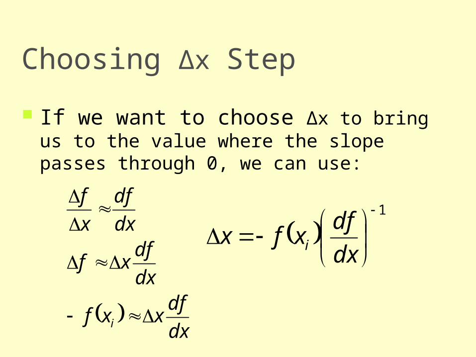
If we want to choose Δx to bring us to the value where the slope passes through 0, we can use:
dx
dfxxf
dx
dfxf
dx
df
x
f
i
1
dx
dfxfx i
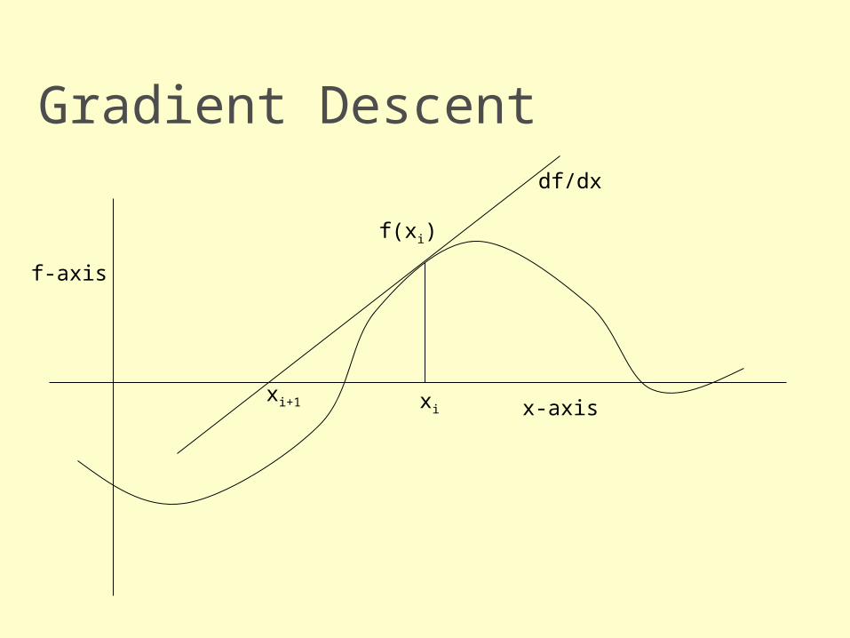
Gradient Descent
f-axis
x-axisxi
f(xi)
df/dx
xi+1
Solving f(x)=g
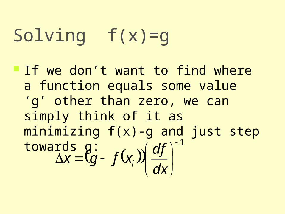
If we don’t want to find where a function equals some value ‘g’ other than zero, we can simply think of it as minimizing f(x)-g and just step towards g:
1
dx
dfxfgx i
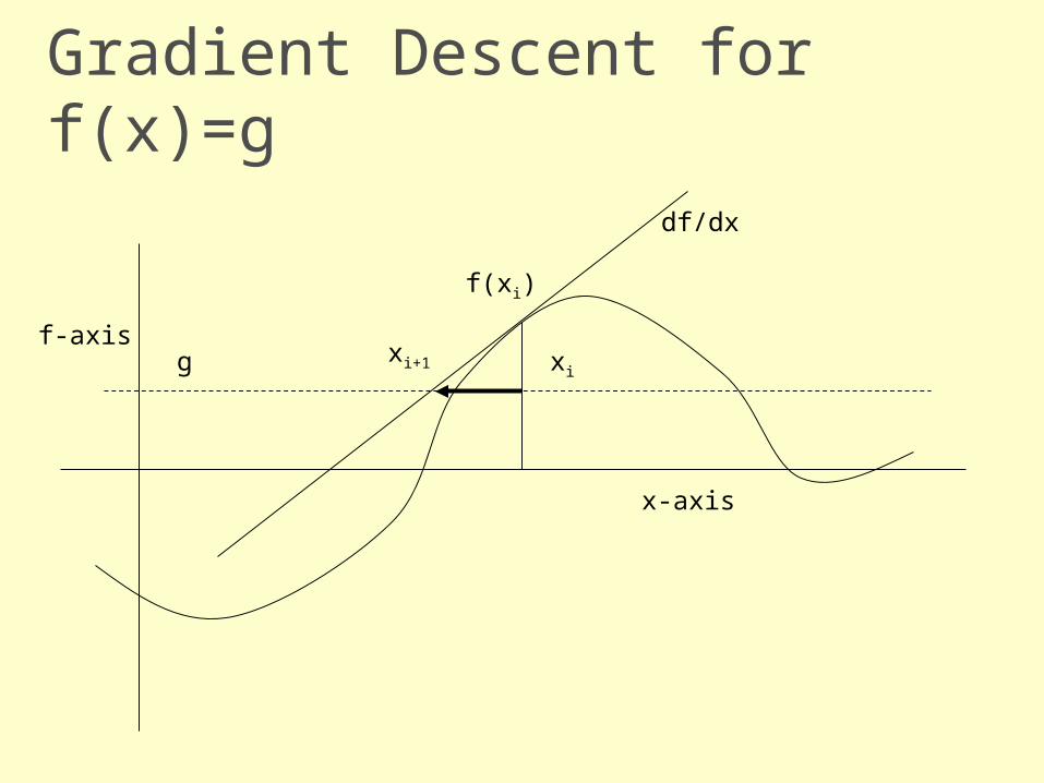
Gradient Descent for f(x)=g
f-axis
x-axis
xi
f(xi)
df/dx
g xi+1
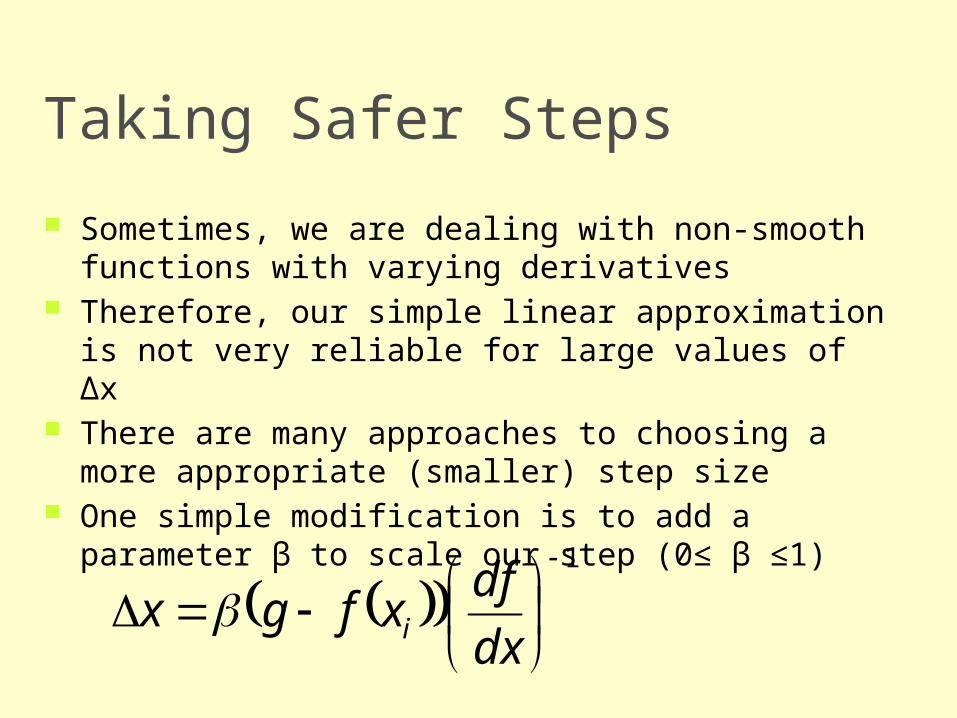
Taking Safer Steps
Sometimes, we are dealing with non-smooth functions with varying derivatives
Therefore, our simple linear approximation is not very reliable for large values of Δx
There are many approaches to choosing a more appropriate (smaller) step size
One simple modification is to add a parameter β to scale our step (0≤ β ≤1)
1
dx
dfxfgx i
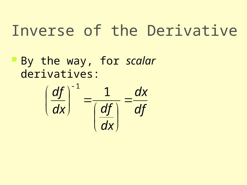
Inverse of the Derivative
By the way, for scalar derivatives:
df
dx
dxdfdx
df
1
1
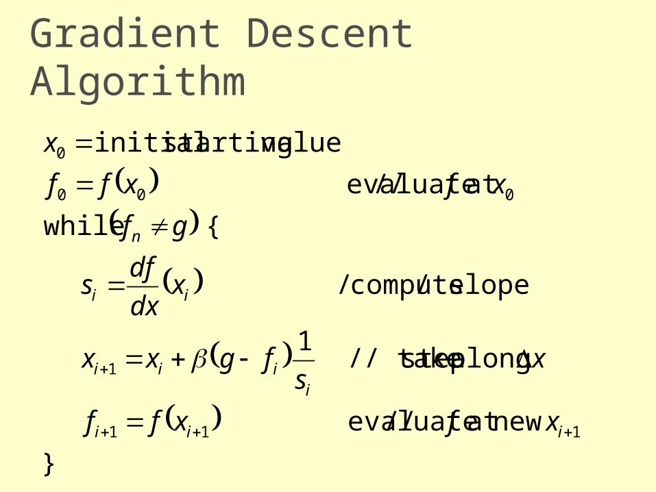
Gradient Descent Algorithm
}
newat evaluate //
along step // take1
slope compute/ /
{ while
at evaluate //
valuestarting initial
111
1
000
0
iii
iiii
ii
n
xfxff
xs
fgxx
xdx
dfs
gf
xfxff
x
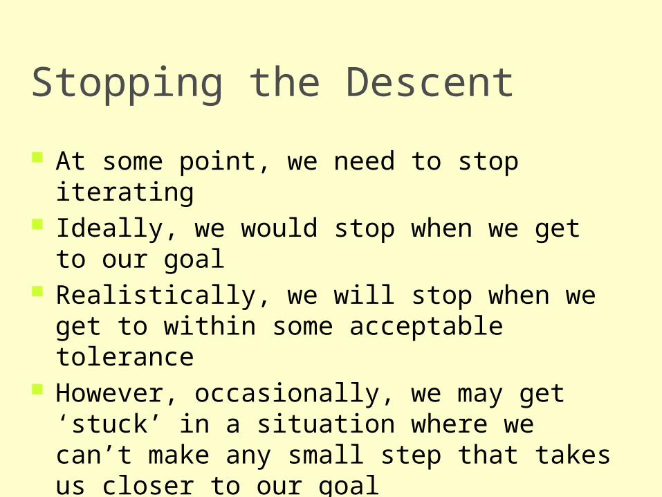
Stopping the Descent
At some point, we need to stop iterating Ideally, we would stop when we get to our goal Realistically, we will stop when we get to within
some acceptable tolerance However, occasionally, we may get ‘stuck’ in a
situation where we can’t make any small step that takes us closer to our goal
We will discuss some more about this later
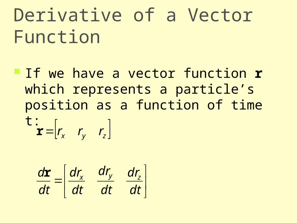
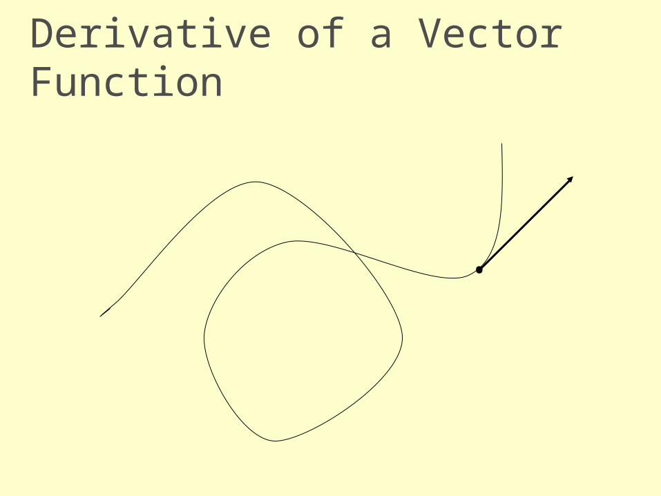
Derivative of a Vector Function
If we have a vector function r which represents a particle’s position as a function of time t:
dt
dr
dt
dr
dt
dr
dt
d
rrr
zyx
zyx
r
r
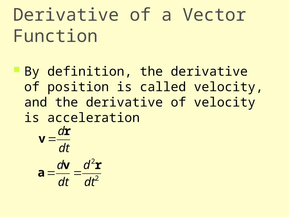
Derivative of a Vector Function
By definition, the derivative of position is called velocity, and the derivative of velocity is acceleration
2
2
dt
d
dt
d
dt
d
rva
rv
Derivative of a Vector Function
•
Vector Derivatives
We’ve seen how to take a derivative of a scalar vs. a scalar, and a vector vs. a scalar
What about the derivative of a scalar vs. a vector, or a vector vs. a vector?
Vector Derivatives
Derivatives of scalars with respect to vectors show up often in field equations, used in exciting subjects like fluid dynamics, solid mechanics, and other physically based animation techniques. If we are lucky, we’ll have time to look at these later in the quarter
Today, however, we will be looking at derivatives of vector quantities with respect to other vector quantities
Jacobians
A Jacobian is a vector derivative with respect to another vector
If we have a vector valued function of a vector of variables f(x), the Jacobian is a matrix of partial derivatives- one partial derivative for each combination of components of the vectors
The Jacobian matrix contains all of the information necessary to relate a change in any component of x to a change in any component of f
The Jacobian is usually written as J(f,x), but you can really just think of it as df/dx
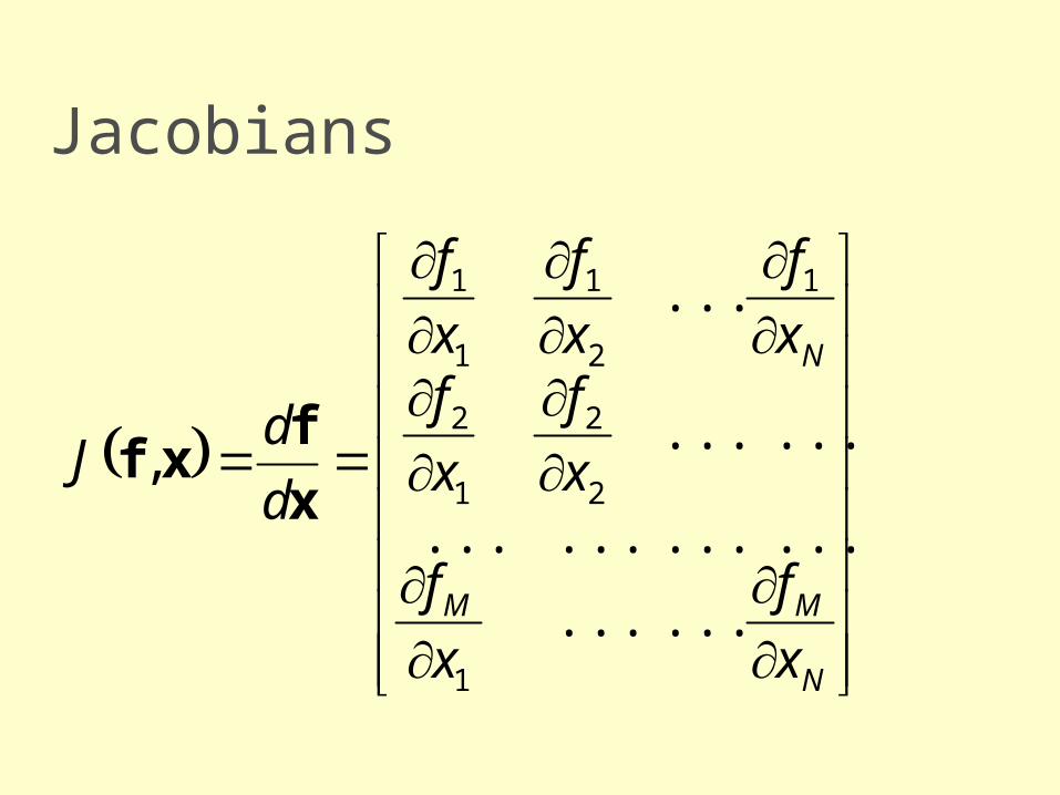
Jacobians
N
MM
N
x
f
x
f
x
f
x
fx
f
x
f
x
f
d
dJ
......
............
......
...
,
1
2
2
1
2
1
2
1
1
1
x
fxf
Partial Derivatives
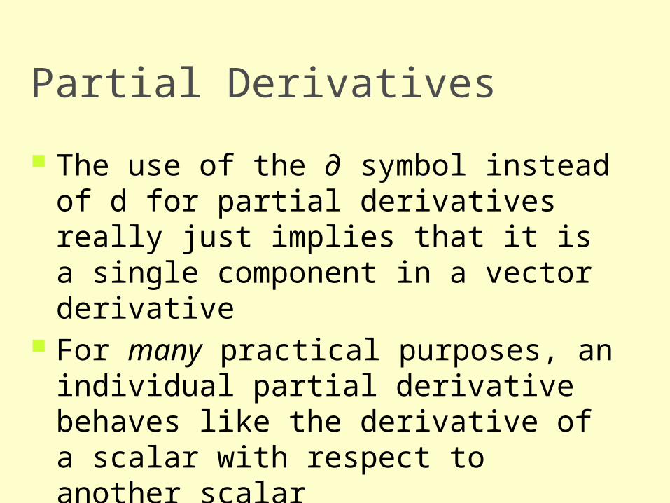
The use of the ∂ symbol instead of d for partial derivatives really just implies that it is a single component in a vector derivative
For many practical purposes, an individual partial derivative behaves like the derivative of a scalar with respect to another scalar

Jacobian Inverse Kinematics
Jacobians
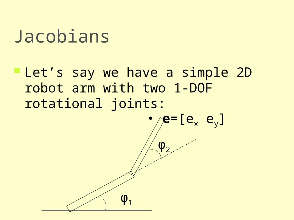
Let’s say we have a simple 2D robot arm with two 1-DOF rotational joints:
φ1
φ2
• e=[ex ey]
Jacobians
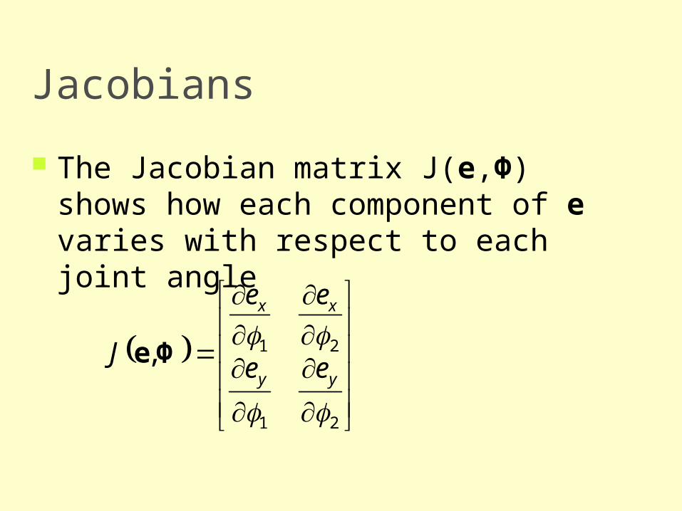
The Jacobian matrix J(e,Φ) shows how each component of e varies with respect to each joint angle
21
21,
yy
xx
ee
ee
J Φe
Jacobians
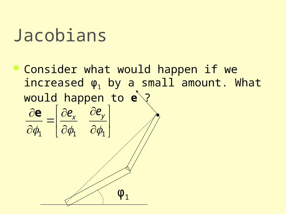
Consider what would happen if we increased φ1 by a small amount. What would happen to e ?
φ1
•
111 yxeee
Jacobians
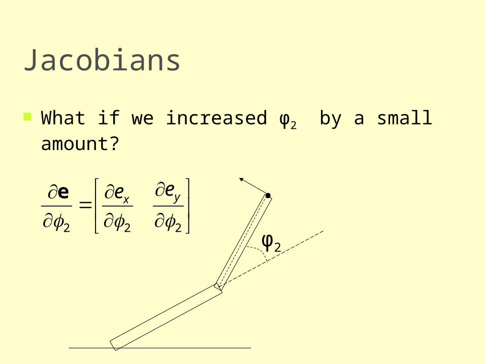
What if we increased φ2 by a small amount?
φ2
•
222 yxeee
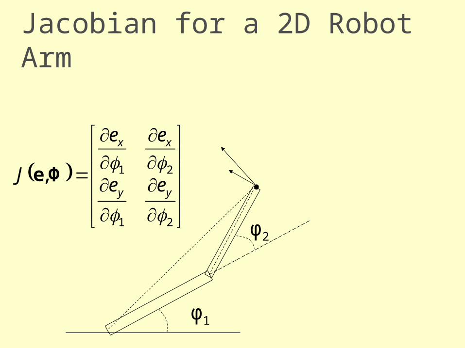
Jacobian for a 2D Robot Arm
φ2
•
φ1
21
21,
yy
xx
ee
ee
J Φe
Jacobian Matrices
Just as a scalar derivative df/dx of a function f(x) can vary over the domain of possible values for x, the Jacobian matrix J(e,Φ) varies over the domain of all possible poses for Φ
For any given joint pose vector Φ, we can explicitly compute the individual components of the Jacobian matrix
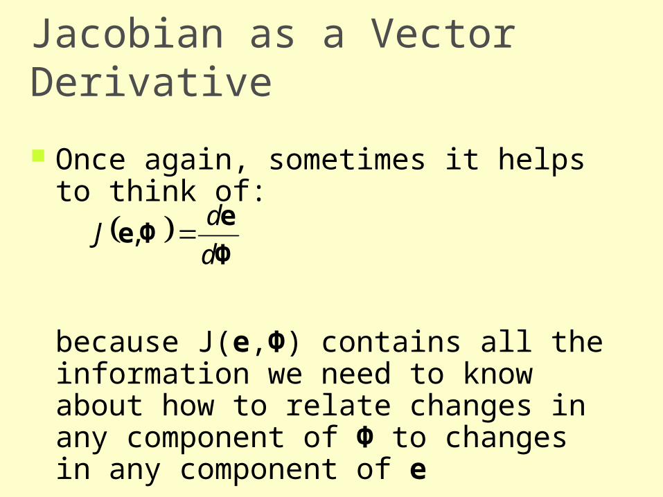
Jacobian as a Vector Derivative
Φ
eΦe
d
dJ ,
Once again, sometimes it helps to think of:
because J(e,Φ) contains all the information we need to know about how to relate changes in any component of Φ to changes in any component of e
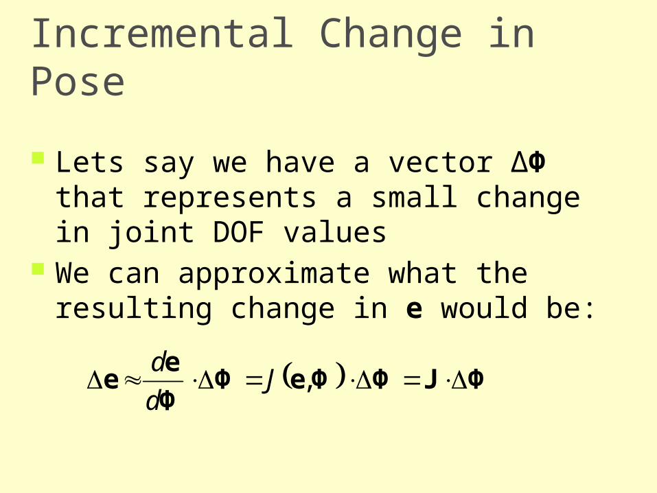
Incremental Change in Pose
Lets say we have a vector ΔΦ that represents a small change in joint DOF values
We can approximate what the resulting change in e would be:
ΦJΦΦeΦΦ
ee ,Jd
d
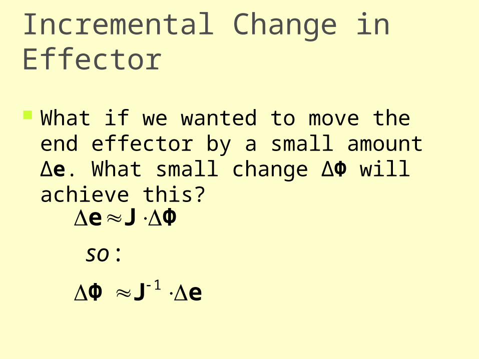
Incremental Change in Effector
What if we wanted to move the end effector by a small amount Δe. What small change ΔΦ will achieve this?
eJΦ
ΦJe
1
: so
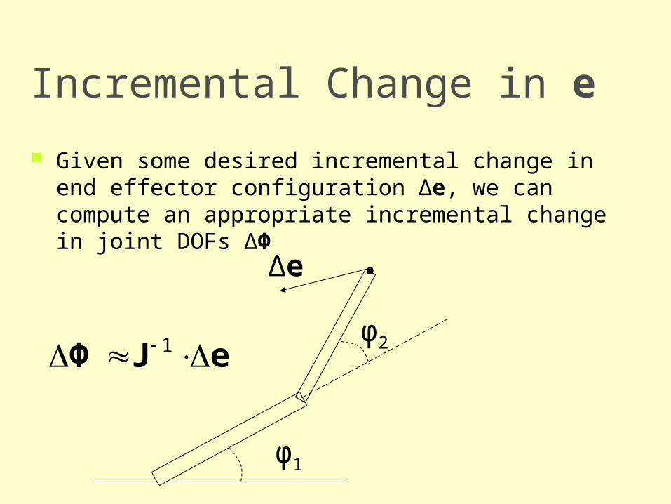
Incremental Change in e
φ2
•
φ1
eJΦ 1
Δe
Given some desired incremental change in end effector configuration Δe, we can compute an appropriate incremental change in joint DOFs ΔΦ
Incremental Changes
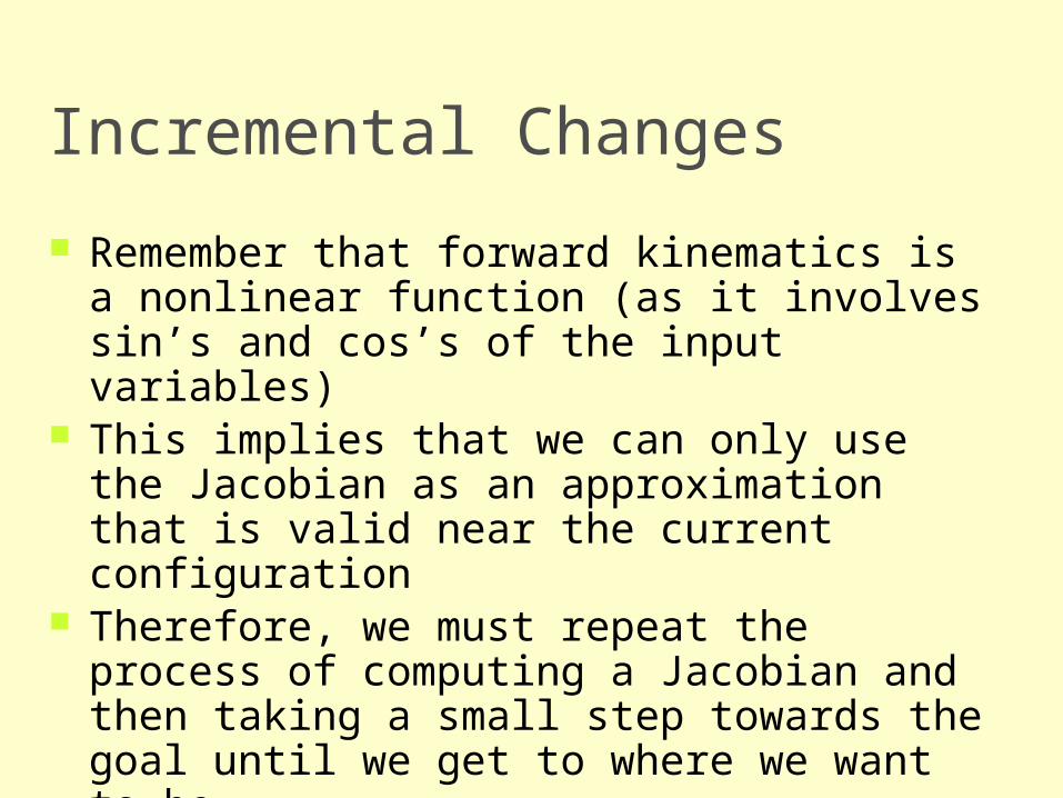
Remember that forward kinematics is a nonlinear function (as it involves sin’s and cos’s of the input variables)
This implies that we can only use the Jacobian as an approximation that is valid near the current configuration
Therefore, we must repeat the process of computing a Jacobian and then taking a small step towards the goal until we get to where we want to be
End Effector Goals
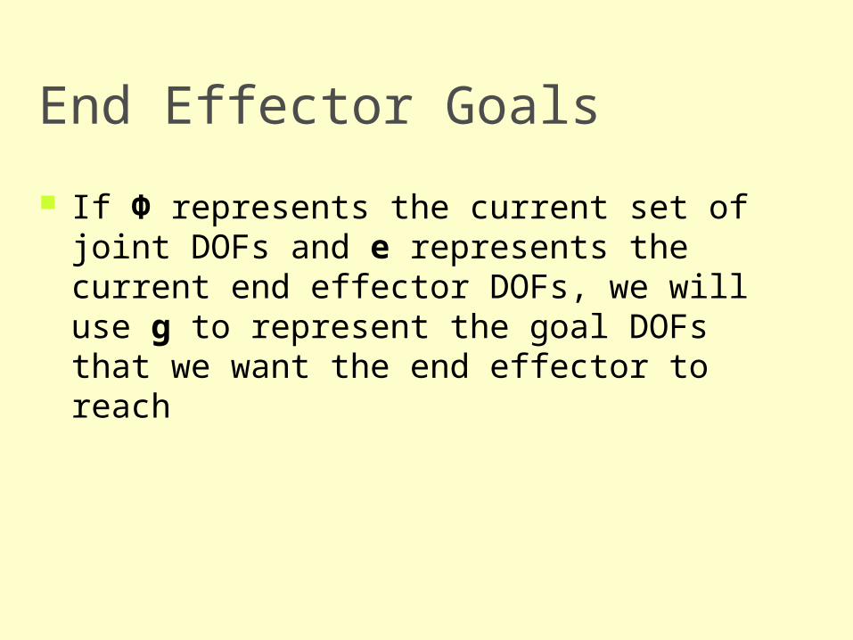
If Φ represents the current set of joint DOFs and e represents the current end effector DOFs, we will use g to represent the goal DOFs that we want the end effector to reach
Choosing Δe
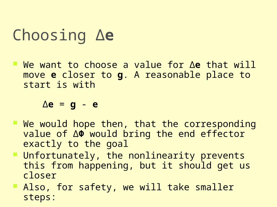
We want to choose a value for Δe that will move e closer to g. A reasonable place to start is with
Δe = g - e
We would hope then, that the corresponding value of ΔΦ would bring the end effector exactly to the goal
Unfortunately, the nonlinearity prevents this from happening, but it should get us closer
Also, for safety, we will take smaller steps:
Δe = β(g - e)
where 0≤ β ≤1
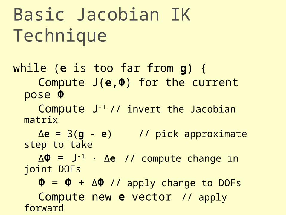
Basic Jacobian IK Technique
while (e is too far from g) {Compute J(e,Φ) for the current pose ΦCompute J-1 // invert the Jacobian matrix
Δe = β(g - e) // pick approximate step to take
ΔΦ = J-1 · Δe // compute change in joint DOFs
Φ = Φ + ΔΦ // apply change to DOFs
Compute new e vector // apply forward// kinematics to see// where we ended up
}
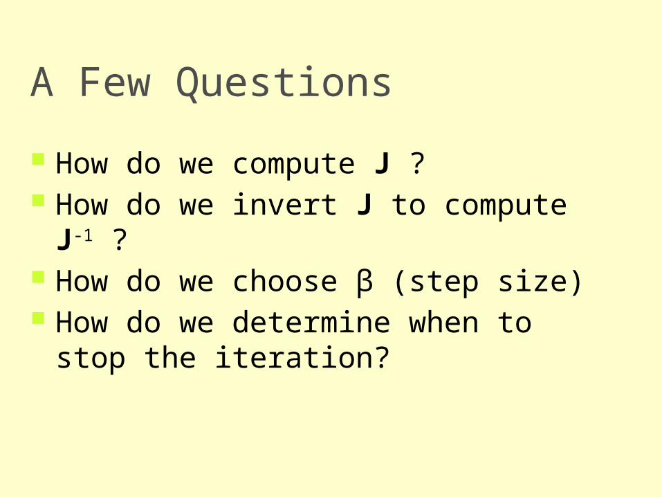
A Few Questions
How do we compute J ? How do we invert J to compute J-1 ? How do we choose β (step size) How do we determine when to stop the
iteration?
Computing the Jacobian
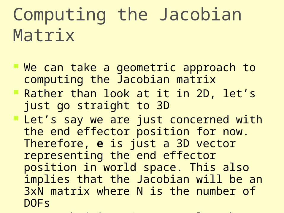
Computing the Jacobian Matrix
We can take a geometric approach to computing the Jacobian matrix
Rather than look at it in 2D, let’s just go straight to 3D
Let’s say we are just concerned with the end effector position for now. Therefore, e is just a 3D vector representing the end effector position in world space. This also implies that the Jacobian will be an 3xN matrix where N is the number of DOFs
For each joint DOF, we analyze how e would change if the DOF changed
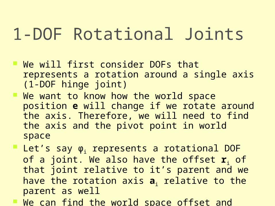
1-DOF Rotational Joints
We will first consider DOFs that represents a rotation around a single axis (1-DOF hinge joint)
We want to know how the world space position e will change if we rotate around the axis. Therefore, we will need to find the axis and the pivot point in world space
Let’s say φi represents a rotational DOF of a joint. We also have the offset ri of that joint relative to it’s parent and we have the rotation axis ai relative to the parent as well
We can find the world space offset and axis by transforming them by their parent joint’s world matrix
1-DOF Rotational Joints
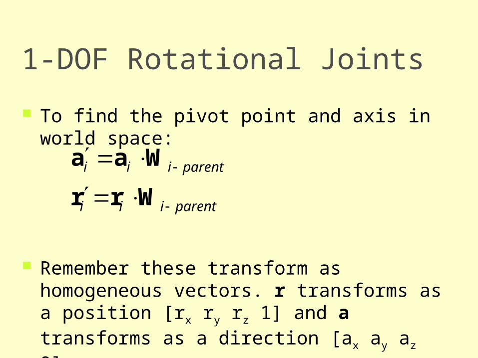
To find the pivot point and axis in world space:
Remember these transform as homogeneous vectors. r transforms as a position [rx ry rz 1] and a transforms as a direction [ax ay az 0]
parentiii
parentiii
Wrr
Waa
Rotational DOFs
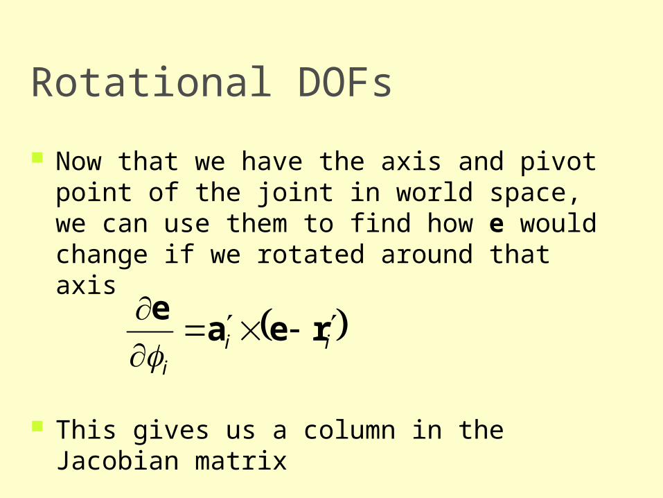
Now that we have the axis and pivot point of the joint in world space, we can use them to find how e would change if we rotated around that axis
This gives us a column in the Jacobian matrix
iii
reae
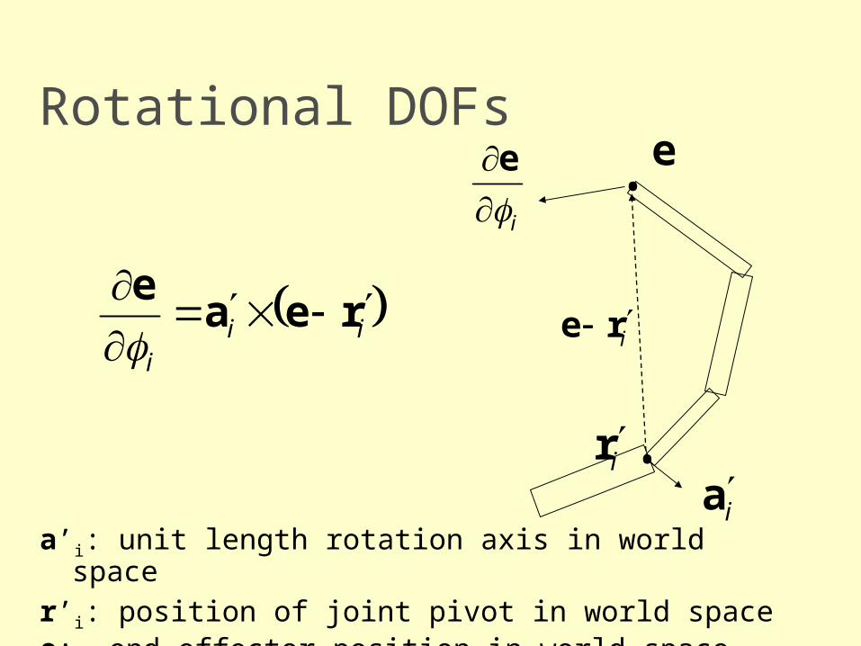
Rotational DOFs
a’i: unit length rotation axis in world space
r’i: position of joint pivot in world spacee: end effector position in world space
iii
reae
•
•i
e
ia
e
ire
ir
3-DOF Rotational Joints
For a 2-DOF or 3-DOF joint, it is actually a little trickier to get the world space axis
Consider how we would find the world space x-axis of a 3-DOF ball joint
Not only do we need to consider the parent’s world matrix, but we need to include the rotation around the next two axes (y and z-axis) as well
This is because those following rotations will rotate the first axis itself
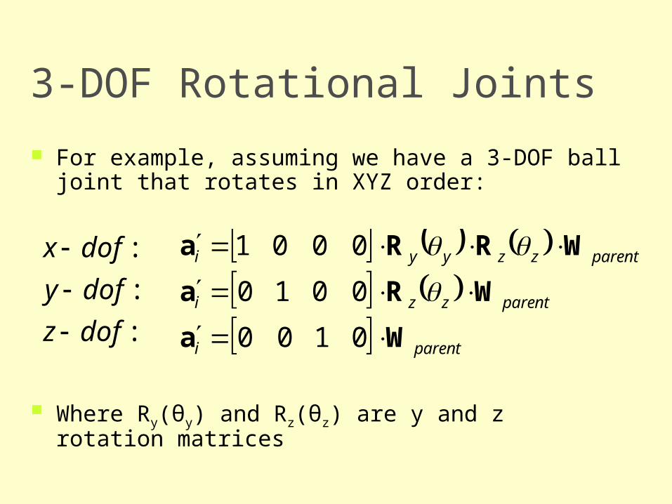
3-DOF Rotational Joints
For example, assuming we have a 3-DOF ball joint that rotates in XYZ order:
Where Ry(θy) and Rz(θz) are y and z rotation matrices
parenti
parentzzi
parentzzyyi
Wa
WRa
WRRa
0100
0010
0001
:
:
:
dofz
dofy
dofx
3-DOF Rotational Joints
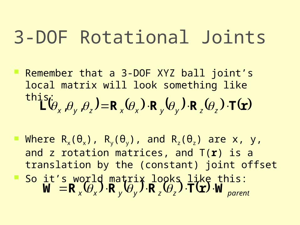
Remember that a 3-DOF XYZ ball joint’s local matrix will look something like this:
Where Rx(θx), Ry(θy), and Rz(θz) are x, y, and z rotation matrices, and T(r) is a translation by the (constant) joint offset
So it’s world matrix looks like this:
rTRRRL zzyyxxzyx ,,
parentzzyyxx WrTRRRW
3-DOF Rotational Joints
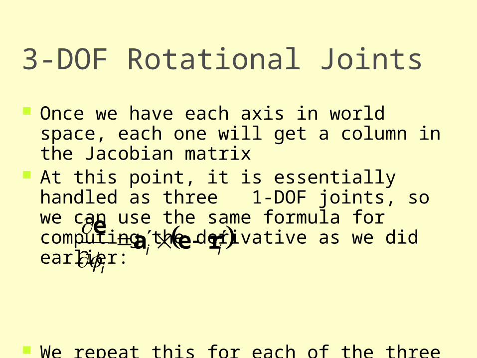
Once we have each axis in world space, each one will get a column in the Jacobian matrix
At this point, it is essentially handled as three 1-DOF joints, so we can use the same formula for computing the derivative as we did earlier:
We repeat this for each of the three axes
iii
reae
Quaternion Joints
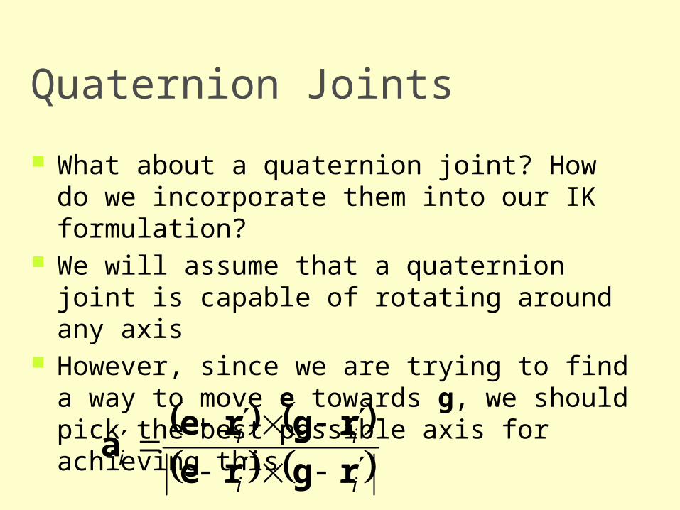
What about a quaternion joint? How do we incorporate them into our IK formulation?
We will assume that a quaternion joint is capable of rotating around any axis
However, since we are trying to find a way to move e towards g, we should pick the best possible axis for achieving this
ii
iii rgre
rgrea
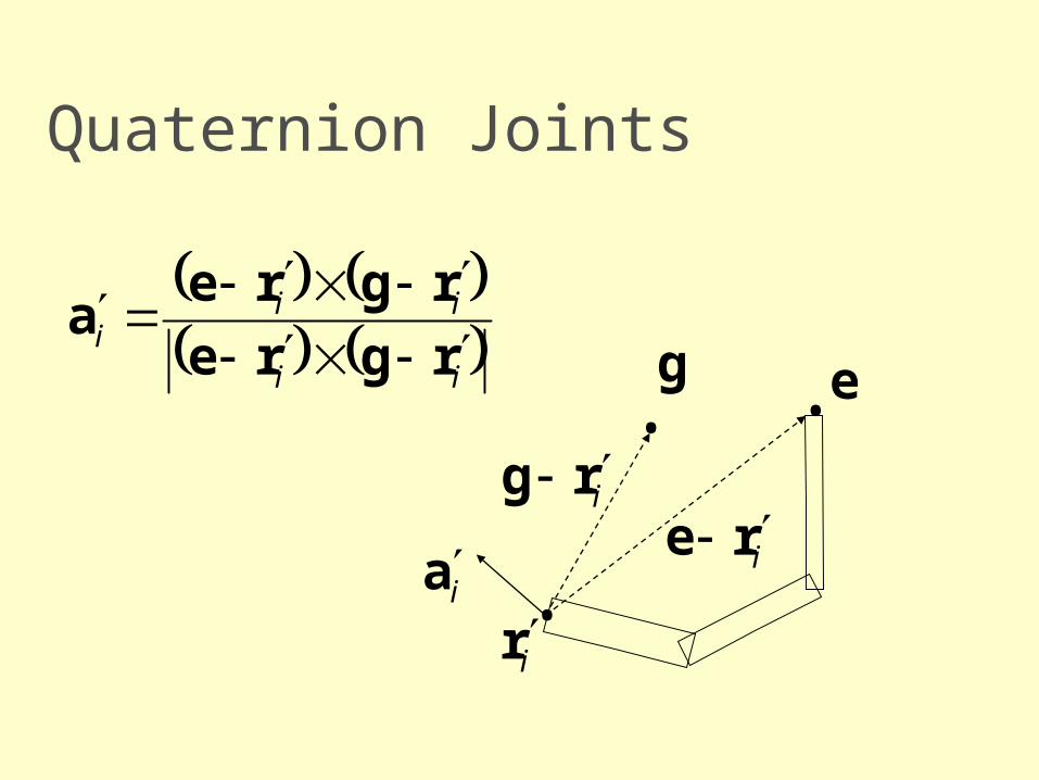
Quaternion Joints
ii
iii rgre
rgrea
•
• •e
irg ire
iria
g
Quaternion Joints
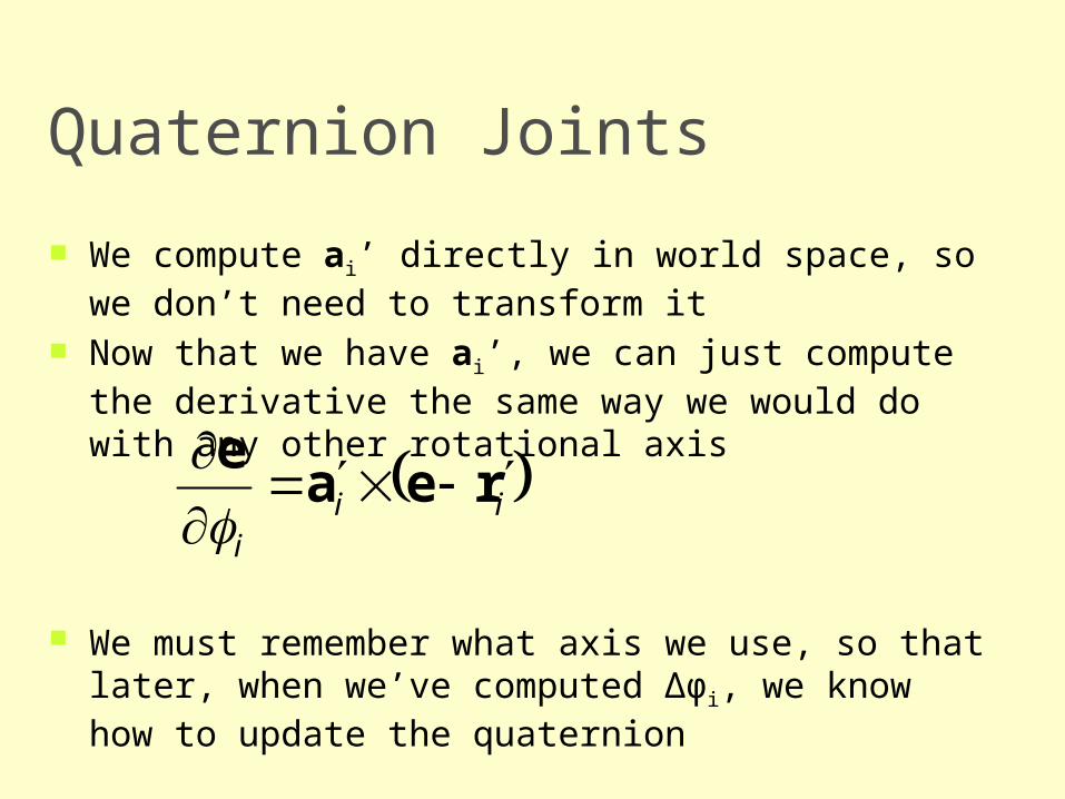
We compute ai’ directly in world space, so we don’t need to transform it
Now that we have ai’, we can just compute the derivative the same way we would do with any other rotational axis
We must remember what axis we use, so that later, when we’ve computed Δφi, we know how to update the quaternion
iii
reae
Translational DOFs
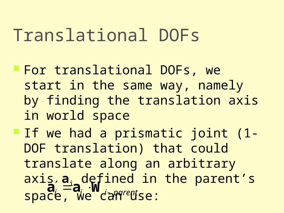
For translational DOFs, we start in the same way, namely by finding the translation axis in world space
If we had a prismatic joint (1-DOF translation) that could translate along an arbitrary axis ai defined in the parent’s space, we can use:
parentiii Waa
Translational DOFs
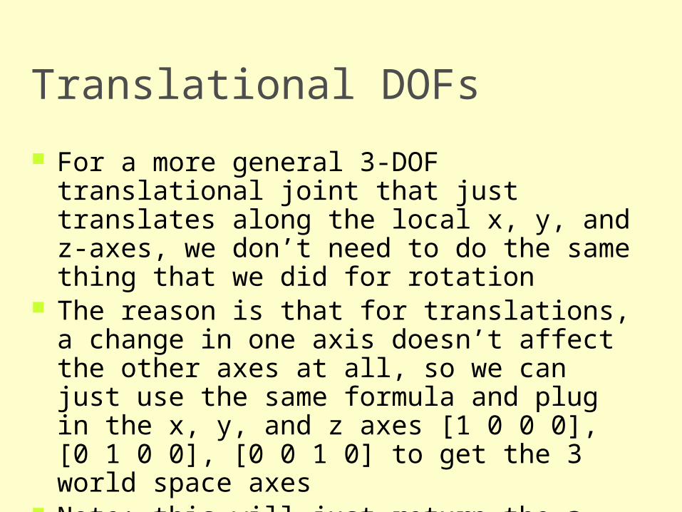
For a more general 3-DOF translational joint that just translates along the local x, y, and z-axes, we don’t need to do the same thing that we did for rotation
The reason is that for translations, a change in one axis doesn’t affect the other axes at all, so we can just use the same formula and plug in the x, y, and z axes [1 0 0 0], [0 1 0 0], [0 0 1 0] to get the 3 world space axes
Note: this will just return the a, b, and c axes of the parent’s world space matrix, and so we don’t actually have to compute them!
Translational DOFs
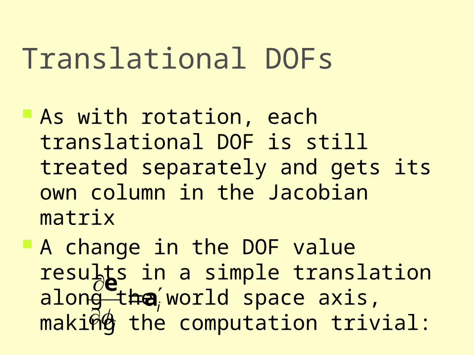
As with rotation, each translational DOF is still treated separately and gets its own column in the Jacobian matrix
A change in the DOF value results in a simple translation along the world space axis, making the computation trivial:
ii
ae
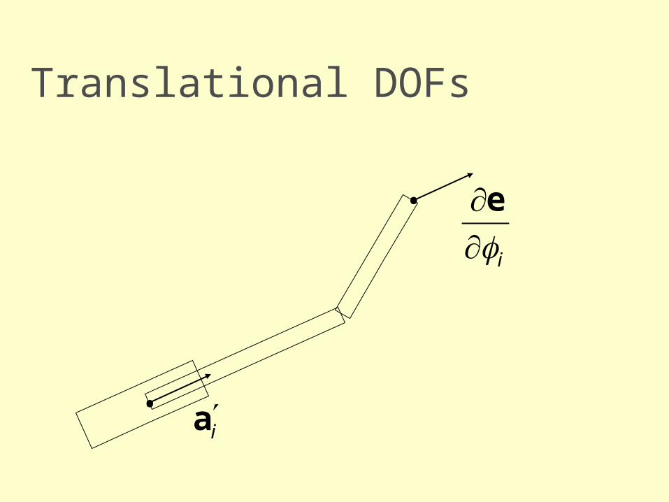
Translational DOFs
ia
ie
•
•
Building the Jacobian
To build the entire Jacobian matrix, we just loop through each DOF and compute a corresponding column in the matrix
If we wanted, we could use more elaborate joint types (scaling, translation along a path, shearing…) and still compute an appropriate derivative
If absolutely necessary, we could always resort to computing a numerical approximation to the derivative
Units & Scaling
What about units? Rotational DOFs use radians and translational
DOFs use meters (or some other measure of distance)
How can we combine their derivatives into the same matrix?
Well, it’s really a bit of a hack, but we just combine them anyway
If desired, we can scale any column to adjust how much the IK will favor using that DOF
Units & Scaling
For example, we could scale all rotations by some constant that causes the IK to behave how we would like
Also, we could use this as an additional way to get control over the behavior of the IK
We can store an additional parameter for each DOF that defines how ‘stiff’ it should behave
If we scale the derivative larger (but preserve direction), the solution will compensate with a smaller value for Δφi, therefore making it act stiff
There are several proposed methods for automatically setting the stiffness to a reasonable default value. They generally work based on some function of the length of the actual bone. The Welman paper talks about this.
End Effector Orientation
End Effector Orientation
We’ve examined how to form the columns of a Jacobian matrix for a position end effector with 3 DOFs
How do we incorporate orientation of the end effector?
We will add more DOFs to the end effector vector e
Which method should we use to represent the orientation? (Euler angles? Quaternions?…)
Actually, a popular method is to use the 3 DOF scaled axis representation!
Scaled Rotation Axis
We learned that any orientation can be represented as a single rotation around some axis
Therefore, we can store an orientation as an 3D vector The direction of the vector is the rotation axis The length of the vector is the angle to rotate in
radians This method has some properties that work well with the
Jacobian approach Continuous and consistent No redundancy or extra constraints It’s also a nice method to store incremental changes
in rotation
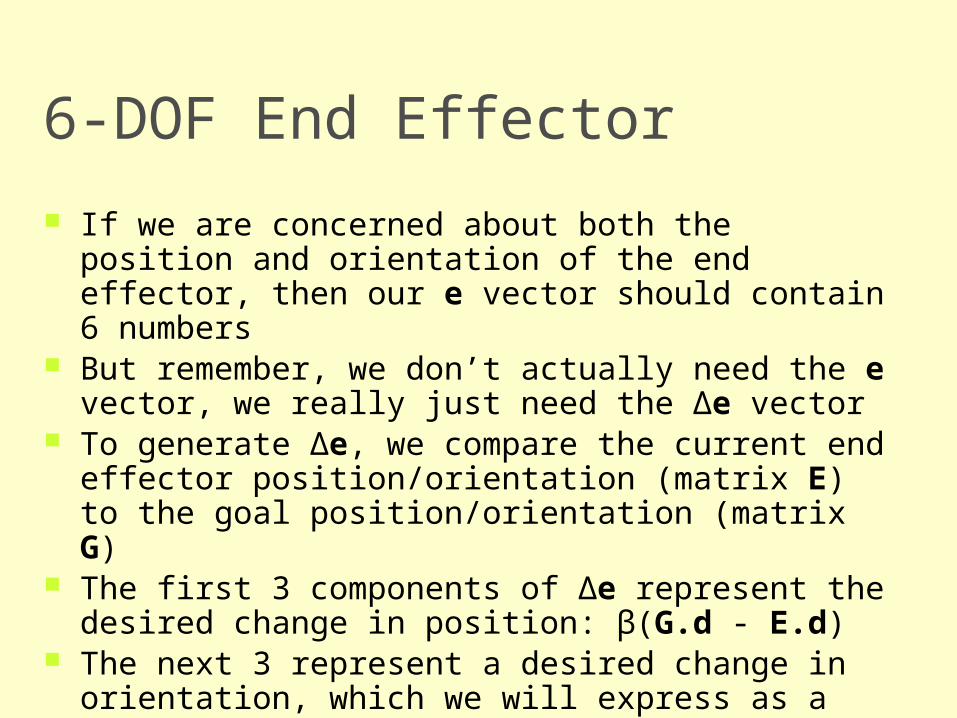
6-DOF End Effector
If we are concerned about both the position and orientation of the end effector, then our e vector should contain 6 numbers
But remember, we don’t actually need the e vector, we really just need the Δe vector
To generate Δe, we compare the current end effector position/orientation (matrix E) to the goal position/orientation (matrix G)
The first 3 components of Δe represent the desired change in position: β(G.d - E.d)
The next 3 represent a desired change in orientation, which we will express as a scaled axis vector
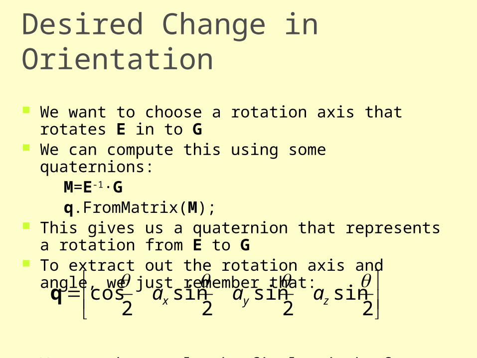
Desired Change in Orientation
We want to choose a rotation axis that rotates E in to G We can compute this using some quaternions:
M=E-1·Gq.FromMatrix(M);
This gives us a quaternion that represents a rotation from E to G
To extract out the rotation axis and angle, we just remember that:
We can then scale the final axis by β
2sin
2sin
2sin
2cos
zyx aaaq
End Effector
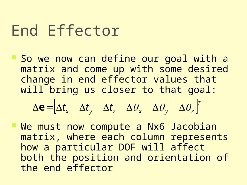
So we now can define our goal with a matrix and come up with some desired change in end effector values that will bring us closer to that goal:
We must now compute a Nx6 Jacobian matrix, where each column represents how a particular DOF will affect both the position and orientation of the end effector
Tzyxzyx ttt e
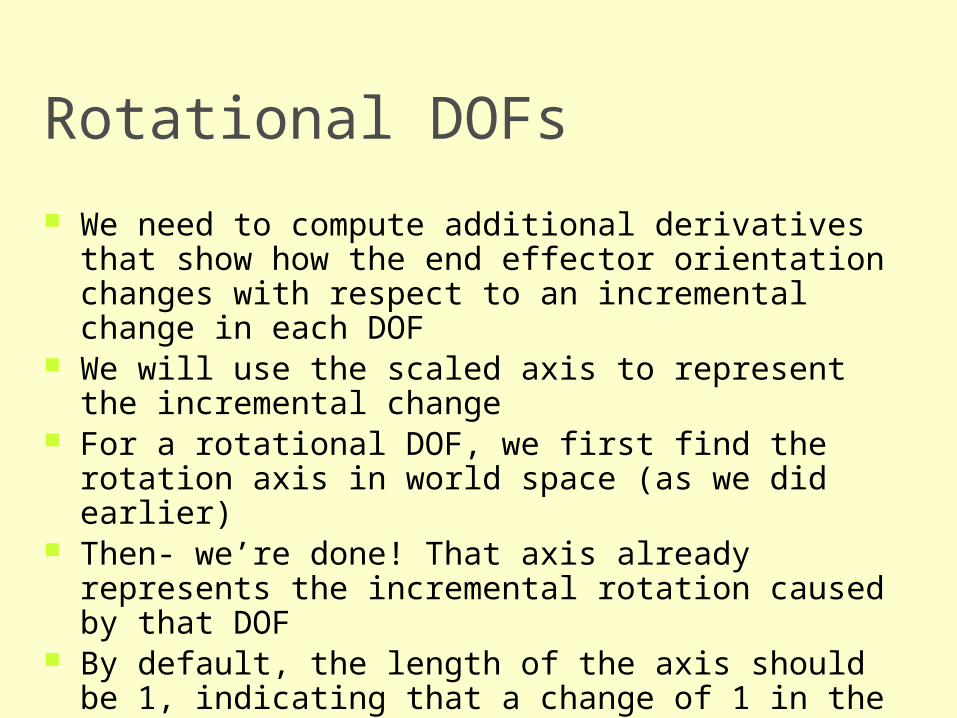
Rotational DOFs
We need to compute additional derivatives that show how the end effector orientation changes with respect to an incremental change in each DOF
We will use the scaled axis to represent the incremental change
For a rotational DOF, we first find the rotation axis in world space (as we did earlier)
Then- we’re done! That axis already represents the incremental rotation caused by that DOF
By default, the length of the axis should be 1, indicating that a change of 1 in the DOF value results in a rotation of 1 radian around the axis. We can scale this by a stiffness value if desired
Rotational DOFs
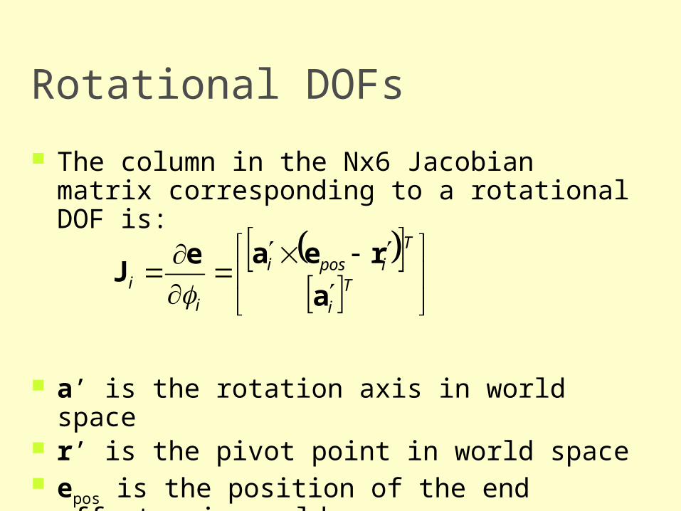
The column in the Nx6 Jacobian matrix corresponding to a rotational DOF is:
a’ is the rotation axis in world space r’ is the pivot point in world space epos is the position of the end effector in world
space
T
i
Tiposi
ii
a
reaeJ
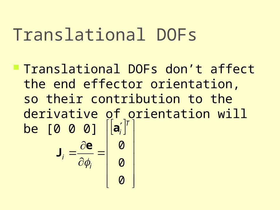
Translational DOFs
Translational DOFs don’t affect the end effector orientation, so their contribution to the derivative of orientation will be [0 0 0]
0
0
0
Ti
ii
a
eJ
Inverse Kinematics (part 2)
CSE169: Computer Animation
Instructor: Steve Rotenberg
UCSD, Winter 2005

Inverting the Jacobian Matrix
Inverting the Jacobian
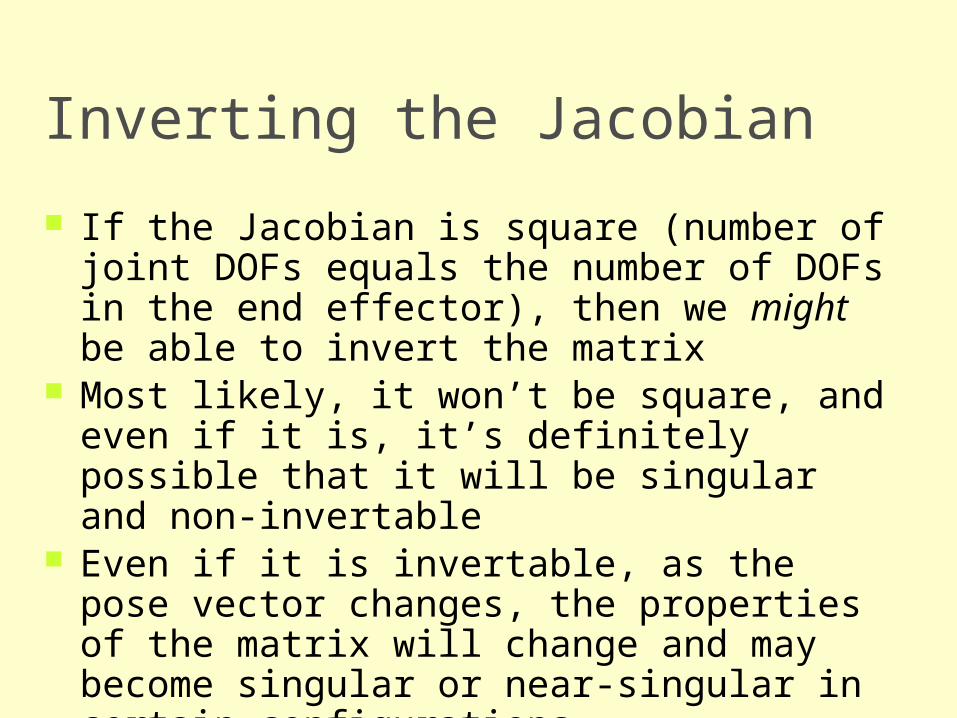
If the Jacobian is square (number of joint DOFs equals the number of DOFs in the end effector), then we might be able to invert the matrix
Most likely, it won’t be square, and even if it is, it’s definitely possible that it will be singular and non-invertable
Even if it is invertable, as the pose vector changes, the properties of the matrix will change and may become singular or near-singular in certain configurations
The bottom line is that just relying on inverting the matrix is not going to work
Underconstrained Systems
If the system has more degrees of freedom in the joints than in the end effector, then it is likely that there will be a continuum of redundant solutions (i.e., an infinite number of solutions)
In this situation, it is said to be underconstrained or redundant
These should still be solvable, and might not even be too hard to find a solution, but it may be tricky to find a ‘best’ solution

Overconstrained Systems
If there are more degrees of freedom in the end effector than in the joints, then the system is said to be overconstrained, and it is likely that there will not be any possible solution
In these situations, we might still want to get as close as possible
However, in practice, overconstrained systems are not as common, as they are not a very useful way to build an animal or robot (they might still show up in some special cases though)
Well-Constrained Systems
If the number of DOFs in the end effector equals the number of DOFs in the joints, the system could be well constrained and invertable
In practice, this will require the joints to be arranged in a way so their axes are not redundant
This property may vary as the pose changes, and even well-constrained systems may have trouble
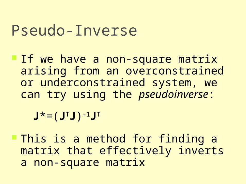
Pseudo-Inverse
If we have a non-square matrix arising from an overconstrained or underconstrained system, we can try using the pseudoinverse:
J*=(JTJ)-1JT
This is a method for finding a matrix that effectively inverts a non-square matrix
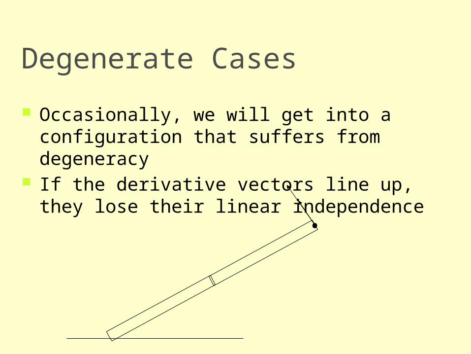
Degenerate Cases
•
Occasionally, we will get into a configuration that suffers from degeneracy
If the derivative vectors line up, they lose their linear independence
Single Value Decomposition
The SVD is an algorithm that decomposes a matrix into a form whose properties can be analyzed easily
It allows us to identify when the matrix is singular, near singular, or well formed
It also tells us about what regions of the multidimensional space are not adequately covered in the singular or near singular configurations
The bottom line is that it is a more sophisticated, but expensive technique that can be useful both for analyzing the matrix and inverting it
Jacobian Transpose
Another technique is to simply take the transpose of the Jacobian matrix!
Surprisingly, this technique actually works pretty well
It is much faster than computing the inverse or pseudo-inverse
Also, it has the effect of localizing the computations. To compute Δφi for joint i, we compute the column in the Jacobian matrix Ji as before, and then just use:
Δφi = JiT · Δe
Jacobian Transpose
With the Jacobian transpose (JT) method, we can just loop through each DOF and compute the change to that DOF directly
With the inverse (JI) or pseudo-inverse (JP) methods, we must first loop through the DOFs, compute and store the Jacobian, invert (or pseudo-invert) it, then compute the change in DOFs, and then apply the change
The JT method is far friendlier on memory access & caching, as well as computations
However, if one prefers quality over performance, the JP method might be better…
Iterating to the Solution
Iteration
Whether we use the JI, JP, or JT method, we must address the issue of iteration towards the solution
We should consider how to choose an appropriate step size β and how to decide when the iteration should stop
When to Stop
There are three main stopping conditions we should account for Finding a successful solution (or close enough) Getting stuck in a condition where we can’t improve
(local minimum) Taking too long (for interactive systems)
All three of these are fairly easy to identify by monitoring the progress of Φ
These rules are just coded into the while() statement for the controlling loop
Finding a Successful Solution
We really just want to get close enough within some tolerance
If we’re not in a big hurry, we can just iterate until we get within some floating point error range
Alternately, we could choose to stop when we get within some tolerance measurable in pixels
For example, we could position an end effector to 0.1 pixel accuracy
This gives us a scheme that should look good and automatically adapt to spend more time when we are looking at the end effector up close (level-of-detail)
Local Minima
If we get stuck in a local minimum, we have several options Don’t worry about it and just accept it as the best we
can do Switch to a different algorithm (CCD…) Randomize the pose vector slightly (or a lot) and try
again Send an error to whatever is controlling the end
effector and tell it to try something else Basically, there are few options that are truly appealing,
as they are likely to cause either an error in the solution or a possible discontinuity in the motion
Taking Too Long
In a time critical situation, we might just limit the iteration to a maximum number of steps
Alternately, we could use internal timers to limit it to an actual time in seconds
Iteration Stepping
Step size Stability Performance

Other IK Issues
Joint Limits
A simple and reasonably effective way to handle joint limits is to simply clamp the pose vector as a final step in each iteration
One can’t compute a proper derivative at the limits, as the function is effectively discontinuous at the boundary
The derivative going towards the limit will be 0, but coming away from the limit will be non-zero. This leads to an inequality condition, which can’t be handled in a continuous manner
We could just choose whether to set the derivative to 0 or non-zero based on a reasonable guess as to which way the joint would go. This is easy in the JT method, but can potentially cause trouble in JI or JP
Higher Order Approximation
The first derivative gives us a linear approximation to the function
We can also take higher order derivatives and construct higher order approximations to the function
This is analogous to approximating a function with a Taylor series
Repeatability
If a given goal vector g always generates the same pose vector Φ, then the system is said to be repeatable
This is not likely to be the case for redundant systems unless we specifically try to enforce it
If we always compute the new pose by starting from the last pose, the system will probably not be repeatable
If, however, we always reset it to a ‘comfortable’ default pose, then the solution should be repeatable
One potential problem with this approach however is that it may introduce sharp discontinuities in the solution
Multiple End Effectors
Remember, that the Jacobian matrix relates each DOF in the skeleton to each scalar value in the e vector
The components of the matrix are based on quantities that are all expressed in world space, and the matrix itself does not contain any actual information about the connectivity of the skeleton
Therefore, we extend the IK approach to handle tree structures and multiple end effectors without much difficulty
We simply add more DOFs to the end effector vector to represent the other quantities that we want to constrain
However, the issue of scaling the derivatives becomes more important as more joints are considered
Multiple Chains
Another approach to handling tree structures and multiple end effectors is to simply treat it as several individual chains
This works for characters often, as we can animate the body with a forward kinematic approach, and then animate each limb with IK by positioning the hand/foot as the end effector goal
This can be faster and simpler, and actually offer a nicer way to control the character
Geometric Constraints
One can also add more abstract geometric constraints to the system Constrain distances, angles within the skeleton Prevent bones from intersecting each other or the
environment Apply different weights to the constraints to signify
their importance Have additional controls that try to maximize the
‘comfort’ of a solution Etc.
Welman talks about this in section 5
Other IK Techniques
Cyclic Coordinate Descent This technique is more of a trigonometric approach and is more
heuristic. It does, however, tend to converge in fewer iterations than the Jacobian methods, even though each iteration is a bit more expensive. Welman talks about this method in section 4.2
Analytical Methods For simple chains, one can directly invert the forward kinematic
equations to obtain an exact solution. This method can be very fast, very predictable, and precisely controllable. With some finesse, one can even formulate good analytical solvers for more complex chains with multiple DOFs and redundancy
Other Numerical Methods There are lots of other general purpose numerical methods for
solving problems that can be cast into f(x)=g format
Jacobian Method as a Black Box
The Jacobian methods were not invented for solving IK. They are a far more general purpose technique for solving systems of non-linear equations
The Jacobian solver itself is a black box that is designed to solve systems that can be expressed as f(x)=g ( e(Φ)=g )
All we need is a method of evaluating f and J for a given value of x to plug it into the solver
If we design it this way, we could conceivably swap in different numerical solvers (JI, JP, JT, damped least-squares, conjugate gradient…)