Sizing storage for Desktop Virtualization - v1 · Sizing storage for Desktop Virtualization Version...

Storage design guidelines

Sizing storage for

Desktop Virtualization

Author(s): Marcel Kleine, Herco van Brug

Version: 1.0

Date: June 4, 2013


Sizing storage for Desktop Virtualization

Version 1.0 June 4, 2013 Page i

© 2013 PQR, all rights reserved.

Niets uit deze uitgave mag worden verveelvoudigd, op geautomatiseerde wijze opgeslagen of openbaar gemaakt in enige vorm of op enigerlei wijze, hetzij elektronisch, mechanisch, door fotokopieën, opnamen of enige andere manier, zonder voorafgaande schriftelijke toestemming van PQR.

No part of this publication may be reproduced, stored in a retrieval system, or transmitted in any form or by any means, electronic, mechanical, photocopying, recording, scanning, or otherwise, without the prior written permission of PQR.



Version 1.0 June 4, 2013 Page ii

DOCUMENT OVERVIEW

REFERENCED DOCUMENTS

Reference Date Description

http://support.microsoft.com/kb/2515143 January 17, 2013

Using Hyper-V™ with large-sector drives in

Windows Server® 2008 and Windows Server 2008

R2 http://technet.microsoft.com/en-us/library/hh831459 February

29, 2012

Hyper-V Support for Large

Sector Disks Overview

http://www.vmware.com/files/pdf/techpaper/Whats-New-VMware-vSphere-51-Storage-Technical-

Whitepaper.pdf

June 2012 What’s New in VMware vSphere® 5.1 –

Storage http://www.netapp.com/us/system/pdf-

reader.aspx?pdfuri=tcm:10-108557-16&m=tr-

4138.pdf

March 2013 Citrix XenDesktop on

NetApp® Storage Solution

Guide http://www.netapp.com/us/system/pdf-

reader.aspx?pdfuri=tcm:10-61632-16&m=tr-3705.pdf

February

2012

NetApp and VMware

View™ Solution Guide

http://support.microsoft.com/kb/2515143

http://technet.microsoft.com/en-us/library/hh831459

http://www.vmware.com/files/pdf/techpaper/Whats-New-VMware-vSphere-51-Storage-Technical-Whitepaper.pdf



http://www.netapp.com/us/system/pdf-reader.aspx?pdfuri=tcm:10-108557-16&m=tr-4138.pdf







Version 1.0 June 4, 2013 Page iii

TABLE OF CONTENTS

1. Why this whitepaper? ....................................................................................................... 1

1.1 Intended audience ........................................................................................................... 1 1.2 Suggestions and improvements ......................................................................................... 1 1.3 Note ................................................................................................................................ 1

2. VDI Variables ................................................................................................................... 2

2.1 Technologies.................................................................................................................... 2 2.2 Reality of VDI deployments ............................................................................................... 3 2.3 Boot storms, logon storms, and steady state ...................................................................... 6 2.4 Without specific requirements ........................................................................................... 7 2.5 Other considerations ........................................................................................................ 8 2.6 IO amplification................................................................................................................ 9 2.7 Stateless versus stateful ................................................................................................. 11

3. Before Storage ............................................................................................................... 12

3.1 Server hardware ............................................................................................................ 12 3.2 Networking and/or Fibre channel fabric ........................................................................... 12 3.3 Conclusion ..................................................................................................................... 15

4. The NetApp storage array ............................................................................................... 16

4.1 NetApp architecture ....................................................................................................... 16 4.2 Read/write ratio ............................................................................................................. 17 4.3 Performance .................................................................................................................. 17 4.4 Processing ..................................................................................................................... 18 4.5 Caching ......................................................................................................................... 19 4.6 Data Footprint Reduction ................................................................................................ 20 4.7 Availability for fault and disaster recovery ........................................................................ 20 4.8 Mixed workloads ............................................................................................................ 21 4.9 Alignment ...................................................................................................................... 21 4.10 Assessments with NetApp ............................................................................................... 22 4.11 The NetApp System Performance Modeler ....................................................................... 22

5. Implementing Storage .................................................................................................... 25

5.1 Validate ......................................................................................................................... 25 5.2 Monitor .......................................................................................................................... 26 5.3 Troubleshooting ............................................................................................................. 27

6. Conclusion ..................................................................................................................... 29

6.1 NetApp array design recommendations ............................................................................ 29

7. More information ............................................................................................................ 30

7.1 About PQR ..................................................................................................................... 30 7.2 Contact.......................................................................................................................... 30 7.3 About the authors .......................................................................................................... 31



Version 1.0 June 4, 2013 Page 1/31

1. WHY THIS WHITEPAPER? When people started building VDI environments, they approached the storage design the same way they had always done with server environments. VDI vendor lab tests gave some indication

about the required IOPS and all was well.

How wrong they were!

As it turned out, the VDI requirements for storage are a world away from server infrastructure requirements. Everything is different as the first VDI projects soon discovered.

Where server infrastructures are pretty constant in their load on the infrastructure, VDI

environments are very wispy in their behavior. Ofcourse there are exceptions but in general, server infrastructures are higher in their demand for storage space than they are for

performance while VDI infrastructures are exactly the other way around. Be aware that this

doesn’t mean that server infrastructures don’t require performance considerations. Especially with disks becoming larger and larger while the IOPS per disk stay the same, the GB/IO ratio is

something to consider in any environment.

But not only was the demand for IOPS a problem, the Read/Write ratio of VDI infrastructure were even worse. Instead of 70/30% R/W% that lab tests had shown, real world scenarios

showed a 15/85% R/W% instead. And since all storage infrastructures to that day were space centric, most were set up with RAID 5 volumes. With the 4x write penalty of RAID 5, the

amount of IOPS fitting on the volumes was much lower than what they intended to deliver had

the VDI workload been read intensive. This means that to deliver the required IOPS (which turned out to be mainly writes), more disks were needed. To add those to the budget after the

project was well underway makes stakeholders very unhappy.

Unfortunately, that’s not the end of the story. Even when IOPS are under control and the amount of spindles has been calculated correctly, still VDI projected failed. It turns out that not

only the amount of IOPS and their read/write ratio was important, also the block size, latency, and several other aspects were exposing new bottlenecks. And with that, the way the different

storage solutions handle different types of workloads, showed once again that not all storage is

created equal and not all VDI deployment models are equal. They all have their specific strengths and weaknesses and require different sizing considerations.

1.1 INTENDED AUDIENCE

This document is intended for Architects, System Administrators, Analysts and IT-Professionals in general who are responsible for and/or interested in designing and implementing storage

solutions for VDI.

1.2 SUGGESTIONS AND IMPROVEMENTS

We did our best to be truthful, clear, complete and accurate in investigating and writing down

the different solutions. Although PQR has a strategic partner relationship with the storage vendor mentioned in this whitepaper our goal is to write an unbiased objective document which

is valuable for the readers. If you have any comments, corrections, or suggestions for improvements of this document, we want to hear from you. We appreciate your feedback.

Please send e-mail to either one of the authors Herco van Brug ([email protected]) and Marcel Kleine

([email protected]) or PQR’s CTO’s Ruben Spruijt ([email protected]) and Jerry Rozeman ([email protected]). Include the product name and version number, and the title of the document in your message.

1.3 NOTE

The intention of this whitepaper is to give insight in how different storage solutions handle the different workloads. As we wrote this whitepaper we sent requests for information to several

vendors. NetApp was the first to respond in the detail level we required for this whitepaper. We started working with that and therefore the first version of this whitepaper includes their

storage solution.

We will keep working with other vendors to get in-depth information about their storage products and we will update this whitepaper when we processed their information.

mailto:[email protected]




2. VDI VARIABLES

When assessing an environment to determine what storage system would fit, we’ve seen there are quite a few variables to take into account. Not all of these variables are directly related to

storage, or even technology. As IT personal we have but one responsibility: providing applications to users, with the required level of availability, performance and with enough

capacity.

Understanding the layers above storage provides an insight on what exactly is coming our way and how it is coming our way. Once we know that – and can still provide availability,

performance and capacity – we are well on our way to a successful project.

Below is an overview of the stack and in the course of the next chapters an overview will be

given of what is important per chapter and how it relates to storage design in general and VDI in particular. This chapter aims to give some insight in most common pitfalls.

A lot of the considerations from this chapter are based on data collected from previous VDI

projects and lab tests. Not all data is extensively explained with graphs and tables; it is to be considered as pragmatic guidelines based on field experience.

2.1 TECHNOLOGIES

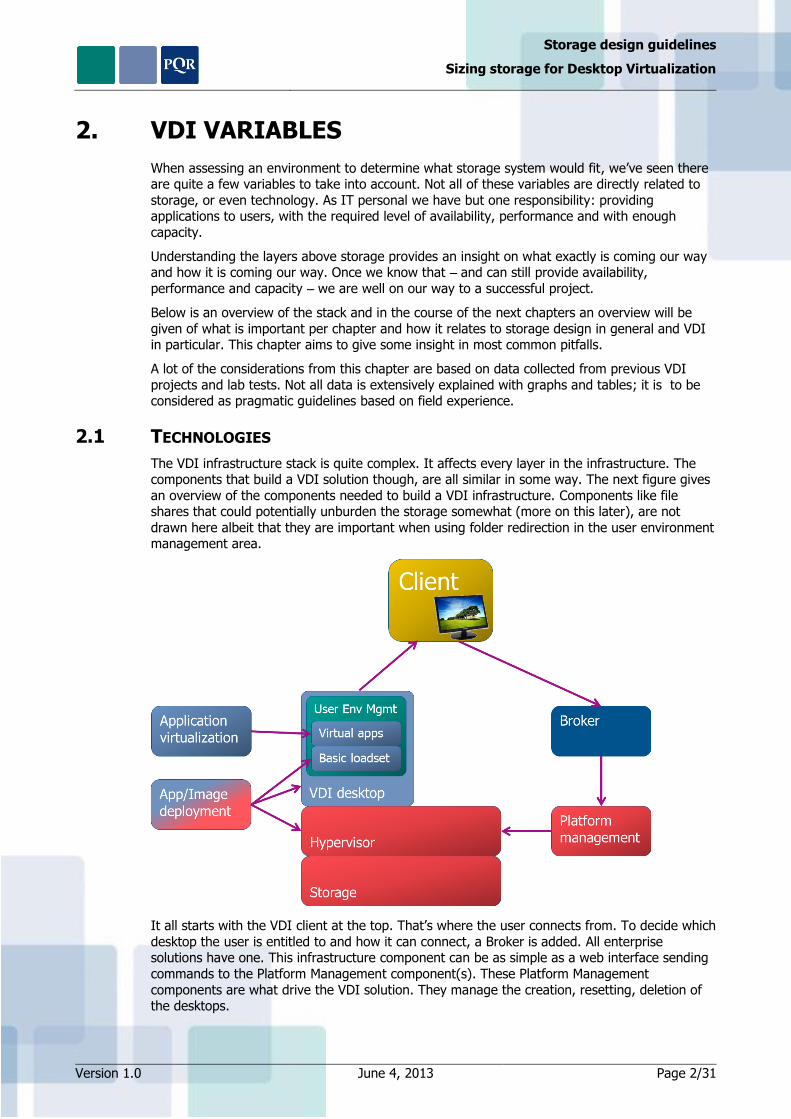
The VDI infrastructure stack is quite complex. It affects every layer in the infrastructure. The components that build a VDI solution though, are all similar in some way. The next figure gives

an overview of the components needed to build a VDI infrastructure. Components like file shares that could potentially unburden the storage somewhat (more on this later), are not

drawn here albeit that they are important when using folder redirection in the user environment management area.

It all starts with the VDI client at the top. That’s where the user connects from. To decide which

desktop the user is entitled to and how it can connect, a Broker is added. All enterprise solutions have one. This infrastructure component can be as simple as a web interface sending

commands to the Platform Management component(s). These Platform Management

components are what drive the VDI solution. They manage the creation, resetting, deletion of the desktops.




All VDI solutions are based on infrastructure components like network, storage, and a hypervisor. Storage can be local to the host or central storage and both can be based on

spinning disks and flash.

Whether the desktops are persistent or non-persistent, they always are based on a master

image containing the basic application loadset and delivered through a deployment mechanism.

They then are filled with (typically) virtual applications that are user and not desktop specific. The final component is the User Environment Management, which regulates everything that the

user needs configured to immediately start working with his or her application. This component also regulates how user profiles are set up and where the user data lands. Folder redirection

especially can greatly decrease the amount of IOPS at login and at steady state, at the expense of the file server.

2.2 REALITY OF VDI DEPLOYMENTS

Starting a VDI project without any resource information about the current infrastructure can be very risky. Even when classifying users correctly into light, medium and heavy user groups, the

applications they use can still put more strain on the infrastructure than anticipated.

A real world scenario is one where 95% of the users were light users in the sense that the average load was only around 3 IOPS. Still, the storage backend was overloaded despite it

being sized for an average of 5 IOPS. The problem was that the light users were playing YouTube movies and Internet Explorer was caching the streams in large 1MB blocks. Those

large blocks were cut down by Windows XP into 64kB blocks and sent to the storage

infrastructure. Where typical VDI IO load (shown in the left picture below) is heavy on 4kB blocks, this stream caching caused a heavy 64kB block profile (right picture below) that the

storage wasn’t designed for.

2.2.1 Typical VDI profile

VDI projects have been around for more than 5 years now. Luckily there’s a trend to be seen

with 9 out of 10 (or perhaps 8 out of 10) projects regarding the load they generate on storage.

If there’s no information on which to base the sizing, these trends are a good starting point. The following graphs show the frontend IOPS generated by a typical VDI infrastructure:




The graph above shows that the typical VDI profile is heavy on writes (85% of all IOPS) and

uses mostly 4kB blocks. Other blocks also occur and make it so the average block size is around 10-12kB. Because of this typical VDI profile nature of almost 100% randomness, the storage

cache has a hard time making sense of the streams and usually gets completely bypassed leading to less than a few percent of cache hits.

If nothing is known about a client’s infrastructure, this may be a good starting point to

prognosticate a new VDI infrastructure. The problem is that a growing percentage of projects don’t adhere to these trends. Some environments have applications that use all resources of the

local desktops. When those are virtualized, they will kill performance.

2.2.2 Typical Office Automation server backend profile

In server backend infrastructures the following graph is more typical.

IOP

S

Block size in kB

Writes

Reads

IOP

S

Block size in kB

Writes

Reads




Sizing for server backends can be just as hard as for VDI. The difference though is that with servers, the first parameter is the size of the dataset they manage. By sizing that correctly

(RAID overhead, growth, required free space, et cetera), the number of hard disks to deliver the needed storage space generally provide more IOPS than the servers need. That’s why a lot

of storage monitoring focuses on storage space and not on storage performance. Only when

performance degrades do people start to look at what the storage is actually doing.

Comparing infrastructures is a dangerous thing. But there is some similarity between the

various office automation infrastructures. They tend to have a 60-70% read workload that has a block size of around 40kB. Because there is some sequentiallity to the data streams the cache

hits of storage solutions average around 30%.

As with VDI, these numbers mean nothing for any specific infrastructure but give some

indication of what a storage solution may need to deliver if nothing else is known.

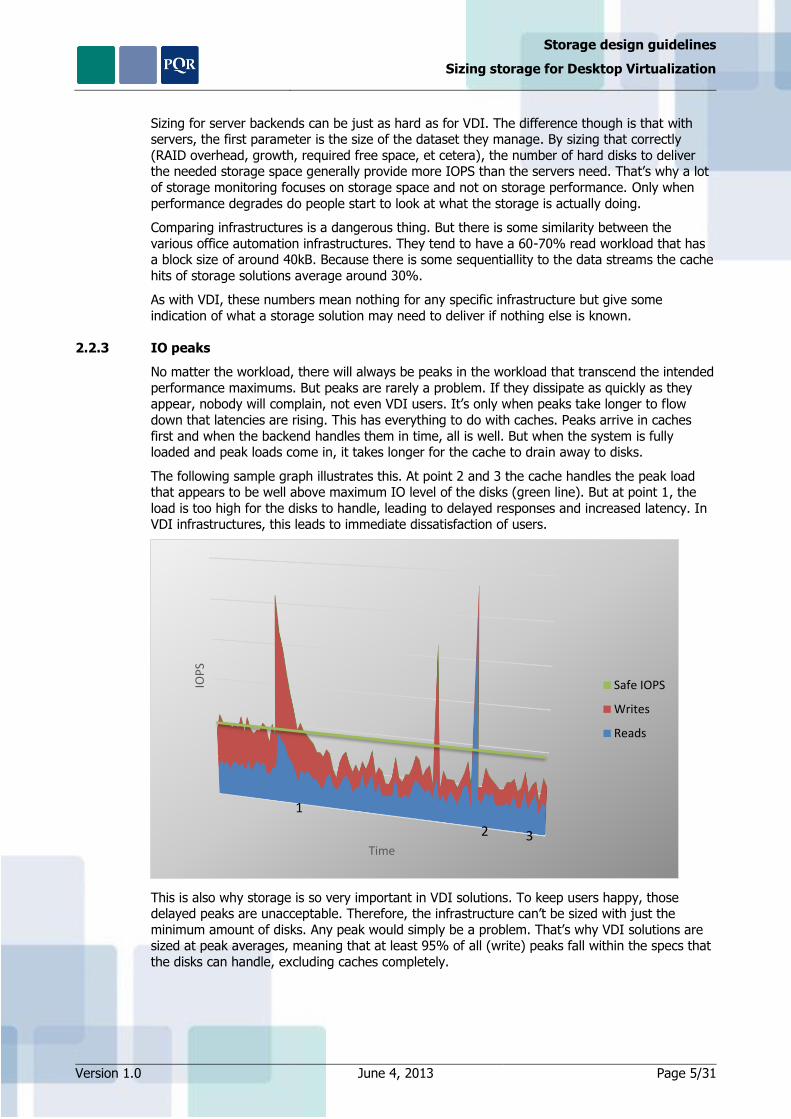
2.2.3 IO peaks

No matter the workload, there will always be peaks in the workload that transcend the intended

performance maximums. But peaks are rarely a problem. If they dissipate as quickly as they appear, nobody will complain, not even VDI users. It’s only when peaks take longer to flow

down that latencies are rising. This has everything to do with caches. Peaks arrive in caches

first and when the backend handles them in time, all is well. But when the system is fully loaded and peak loads come in, it takes longer for the cache to drain away to disks.

The following sample graph illustrates this. At point 2 and 3 the cache handles the peak load that appears to be well above maximum IO level of the disks (green line). But at point 1, the

load is too high for the disks to handle, leading to delayed responses and increased latency. In VDI infrastructures, this leads to immediate dissatisfaction of users.

This is also why storage is so very important in VDI solutions. To keep users happy, those delayed peaks are unacceptable. Therefore, the infrastructure can’t be sized with just the

minimum amount of disks. Any peak would simply be a problem. That’s why VDI solutions are sized at peak averages, meaning that at least 95% of all (write) peaks fall within the specs that

the disks can handle, excluding caches completely.

IOP

S

Time

Safe IOPS

Writes

Reads

1

2 3




2.3 BOOT STORMS, LOGON STORMS, AND STEADY STATE

Everybody that has been dealing with VDI the last few years, knows that it is heavy on writes.

Yet, when VDI projects first started, white papers stated the contrary, predicting a 90% read

infrastructure.

The main reason for this was that they were looking at a single client. When they measured a

single VDI image they observed a picture somewhat like this:

The graph above shows the IO load of a single VDI desktop (as seen on the VDI desktop). On the left there’s a high, read IO load (up to several 100s of IOPS) of the boot of the OS. Then

the user logs in and a 60% read at about 50 IOPS is seen. Then the user starts working with

about 5-10 IOPS at 85% writes for the rest of the day.

Logon storms are often considered problematic. In reality though, only 3% to sometimes 5% of

all users log on simultaneously. That means that the heavy reads of those 3% of users somewhat dissipate against the normal (steady state) operation of everybody else that uses the

infrastructure. In practice, the peak logon at 9 a.m. observed in most VDI infrastructures uses

around 25% extra IOPS, still in the same 15/85% R/W ratio!

That’s why VDI guidelines state that for light, medium and heavy users, the IOs needed are 4,

8 and 12 respectively, and an additional 25% for peak logon times. Sizing for 1000 users at 80% light and 20% heavy would require the storage infrastructure to deliver:

1000 * (80% * 4 + 20% * 12) * 125% = 7000 IOPS at 15% reads and 85% writes.

And that’s it.

Logon storms induce the 25% extra load because of the low concurrency of logons, and boot

storms are taking place outside of office hours. The rest of the day is just steady state use of all the users.

The next factor is boot storms. This introduces a whole new, very heavy read load to the storage although read caches on the host may greatly reduce the reads that need to come from

the array and Citrix PVS can eliminate all reads at boot by caching them for all desktops in the

PVS server’s memory.

When done during office hours, the boot storm has to take place in cache or it will become

unmanageable. If possible, it is best practice to keep the boots outside office hours. That also means that cool features like resetting desktops at user logoff, have to be used sparsely. It’s

IOP

S

Time

Reads

Writes

Steady State

Logon

Boot




recommended to leave the desktop running for other users and only reboot at the night. Even with local read cache on hosts, the boot that takes place during office hours will not be

precached and will flush the cache instead. Only when all desktops boot at once can these caches actually help. So if boot storms need to be handled during office hours (consider 24-

hour businesses), it’s better to have them all boot at once rather than have them all boot in

turns. This will increase processor and memory usage but the performance impact on storage will not just slow it down, it may actually render the storage infrastructure completely unusable.

But in most environments, it is best practice to boot all machines before the users log in. This means that the OS doesn’t have to boot in 30 seconds but it can take much longer, as long as

it’s done by the time the first user arrives. Be aware that it’s also best practice to avoid booting after a user logs off. In environments where users log in and out of different end points, their

desktops preferably stay on in between. If a reboot is performed each time a user logs off, the

strain on the storage would be much higher. Try to avoid boots during office hours.

2.4 WITHOUT SPECIFIC REQUIREMENTS

While it may seem that assessing the current infrastructure for resources will give a closing

overview of the required resources, it’s not as conclusive as it may seem. Assessment tools capture samples at varying intervals. This means that the load at exactly the sample time is

captured but any variations between samples are lost. Statistically, if you take enough samples (300-500 should be a good start), the average will be representative for the load. The same

goes for the amount of desktops measured. Sampling 10 clients doesn’t mean a thing when the

project needs to scale to 1000 clients. The number of clients and the clients themselves should be a very close representation of the total diversity of clients. Only then will assessments give

any usable indication of the resource usage of all clients when extrapolated.

When measuring disk performance, these tools are measuring a number of performance

counters. These then get presented as two distinct numbers: throughput and IOPS.

Assess current infrastructure, spot the difference (services and applications that will not run in

the new infrastructure, upgrades of the Windows platform, new virus scanners, adding

application virtualization, introducing profile management, introducing dynamic provisioning, et cetera).

Light, middle and heavy users concerning backend (Exchange Servers, file servers, database servers) and VDI!

2.4.1 Assessment tools

To get a feel for the resources the current infrastructure requires, there a lot of assessment tools out there. VMware and Microsoft have tools to look at current server and client resources

and calculate the peak usage at different times a day. Both calculate the minimum server hardware to virtualize the measured values by smart interpolation and optimization for their

own virtualization platform. Other tools like Novell’s Platespin Recon can do the same but for

both platforms.

Tools like Liquidware Labs’ Stratusphere can get even more insight into desktop resources and

provide a good indication of how well they would behave when virtualized, even on a per-application basis. The NetApp SPM VDI tool accepts a custom NetApp report in Liquidware Labs

Stratusphere as input. Vendors are making an effort to give much more detail to size VDI.

All these tools though, sample data at specific intervals. Any peaks that occur in between these

intervals will be lost. Whether it’s at 5 minutes or 1 hour intervals doesn’t really matter, peaks

may be short enough to be missed by even 1 second intervals.

All this comes down to statistics. If you sample long enough you’ll probably find enough peaks

to get them in ratio to the overall load. Extrapolating that will give a good probability that it’s close to reality. Also, the law of the large numbers counts here more than anywhere else.

Sampling needs to be representative, across a large enough cross section of the company and




have at least a couple of 100 samples to be statistically valid. But when designing storage, one should always be aware that all assessment tools do is give an indication of reality.

In the end, all the assessment tools do is to provide some indication of the current load. It can still deviate substantially, at least substantially enough to run into trouble once everything is

running off the beautifully designed storage solution. It’s a design matter how much headroom

needs to be calculated in to feel save. And even then, there should always be room to add more if things, despite all of everybody’s best efforts, turn out for the worst.

2.5 OTHER CONSIDERATIONS

But it’s not all about IOPS. There are several other factors that need to be addressed when designing a storage solution.

While all focus on VDI projects seem to go to the delivery of as many IOPS as possible, the virtual desktops also have to land somewhere on disk. When using spindles to deliver IOPS, the

factor IO/GB of a rotating disks is usually low enough that space isn’t an issue. E.g. with 1000 users, needing 10 IOPS per user means that at 80 IOPS per disk in a RAID 1 set, a storage

solution would need 126 disks. With 300GB / disk in RAID 1 that system would give almost

19TB of storage space or 19GB per user. In most VDI infrastructures that’s far more than (non-persistent) user desktops actually need.

To get a feel for the amount of storage that a user desktop needs, the following breakdown has been created. The User, System and Hypervisor layer each need a specific amount of space.

The following picture gives an overview of the sizing of the three different layers. This is

somewhat of a worst-case scenario since not all solutions require a 3D footprint or a spooler that should be able to print 100 pages of a PDF file. Some non-persistent deployments show

that the user and system buffer is hardly used, the desktops use reservations and policies and application deployments don’t apply. In that case the desktops could fit in just under 3GB a

piece. Also, with user data put on CIFS shares (folder redirection), the amount of data per desktop can decrease too. But in general, the space needed to store desktops is built from the

following components:




That means that for 1000 users, at 6.7GB each, the storage system needs 7TB of space. Hosting that in SLC flash disks of 200GB, even in RAID 5, would mean the storage system

needs 48 SSDs. With a practical 20000 IOPS per disk, it will never run out of IOPS, provided that the backplane of the storage solution can handle those 48 disks. Just adding SSD’s to an

array is dangerous though. With the heavy write workload and no intelligence to coalesce IOs

other than the controller does on the SSDs themselves, the life expectancy of those SSDs can be quite low. The whitepaper

http://www.pqr.com/images/stories/Downloads/whitepapers/spinning%20out%20of%20control.pdf explains this in more detail.

It’s important to note where the actually IOPS is happening. While the boot and logon storms are mainly read from and written to the C: drive, the steady state shows a different picture.

Only a few percent of the IOPS still takes place on the C: drive and the rest of the IOPS are

divided equally between the user’s profile and his or her applications.

It may seem to make sense to use some form of auto tiering. This would effectively combine

the IOPS of the SSD’s with the space of HD’s. Unfortunately, all solutions have a scheduled auto tiering principle, meaning that once a day they evaluate hot blocks and move them (usually in

large blocks of multiple dozens of MB’s) to and from SSD’s and HD’s. But when cloning all the

desktops at night, all blocks are hot and need to land in SSD and before they get evaluated, they’re already cleaned up. Solutions that do this inline in either the broker software or the

storage don’t exist yet (H1-2013).

2.6 IO AMPLIFICATION

VDI master images are usually tuned to request as little IOPS as possible. Practice shows that

this can save up to 50% of all IOPS on the infrastructure. But just obtaining savings on the VDI desktop isn’t enough. There are all kinds of factors that amplify the amount of IOPS actually

being requested from the storage.

2.6.1 Linked clones and differencing disks

Until ESX 5.0, the grain size for linked clones was 512 bytes. That means that when a 512 byte

IO comes in, it gets written. When the next IO is 4kB, it gets written right behind the previous 512 byte block. That means that almost all IOs from linked clones are misaligned.

In ESX 5.1, the grain size has been made configurable and defaults to 4kB for redo logs and linked clones. This means that all blocks are at least aligned at 4kB boundaries. If the storage

uses 4kB blocks too then this means that alignment fits perfectly with linked clones. This means

a significant reduction of storage IOs at the cost of the wasted space of blocks smaller than 4kB.

The following figure shows the misalignment of Sparse files (ESXi 5.0 and earlier). The exact same problem occurs in Hyper-V 2008 R2 and earlier as it only supports small-sector disks (512

bytes) for VHDs.

http://www.pqr.com/images/stories/Downloads/whitepapers/spinning%20out%20of%20control.pdf





The next figure shows the improvement of SE sparse files in ESXi 5.1. This too is now supported by Hyper-V 2012 because it now supports large-sector disks.

2.6.2 Profile management storage considerations

Another factor that influences where IOs land is profile management. When parts of profiles are removed from the default location, the system disk may get some leniency and may see a 30%

drop in write IOPS. The solution that serves the profiles however (like a file server) sees about

the same amount of write as the system disk does! That means that profile management increases the total amount of IOPS to the whole system by about 50% as seen from the VDI

desktop.

But file servers handles IOs differently and have their own file system cache. The data usually

lands on a pool different from where VDI desktops land. The advantages in manageability when using profile-management solutions usually outweigh the increase in IOPS but it’s something to

keep an eye on.

2.6.3 Application virtualization

Phase 4 of Project VRC (www.projectvrc.com) shows that the IO impact of application

virtualization. The impact of some solutions are very substantial as the total amount of users that fit on a (VRC) standard box decreases by 10% to sometimes 40%. The impact on storage

however is quite substantial too. Introducing application virtualization may decrease the reads

by some 20% but introduces an increase of 20% in writes.

2.6.4 Virus scanners

In Phase 5 of Project VRC (www.projectvrc.com) the impact of virus scanners was investigated. The impact on IOs is depending heavily on the chosen product. Some products may even be

disqualified as a proper VDI solution because of the 300-400% increase in IOPS they cause. The increase in read IOPS ranges from negligible to almost 50% while the increase in wSrites

averages out at around 15%. This means that antivirus is a definite factor to take into account

when sizing storage for VDI.

2.6.5 Deployment methods

There are three factors that introduce additional VDI load on the storage infrastructure apart from steady state use. The steady-state factor is just the read and write load of when all users

are just using the infrastructure. Then, there are logon storms, boot storms, and deployments.

Logon storms introduce some additional load (some 25%, see chapter 2.3) but do not introduce a different profile as long as the logon concurrency is less than some 5%. Boot storms are best

done outside office hours to make them manageable (see chapter 2.3).

The last factor is deployment. When desktops are deployed by cloning or linked cloning, there is

a lot of large writes coming to the storage. When they are deployed on-the-fly like Citrix’

Provisioning Services (PVS) does, they don’t get deployed before the machine boots, but as the machine boots. That means that with PVS, the deployment (of the write cache differencing

disks) and boot storm happen simultaneously, something that should be avoided during office hours. There’s no point in caching those IOs in a local cache as the majority of the IOPS are

writes which in these deployments are all quite unique.

Other methods like VMware’s linked cloning or Citrix Machine Creation Service (MCS) use

comparable techniques of making a differencing disk that contains the unique properties of a

desktop from a master image.

http://www.projectvrc.com/

http://www.projectvrc.com/




All these methods however increase the IOPS the desktops need once they’re in use.

LAYERING

Whether it’s Citrix Personal vDisk (PVD), Unidesk, or VMware linked clones, all IOs that go into a desktop built with these segmentations, needs to read several layers’ indexes before it knows

where to read or write. That means that all these technologies increase the IOPS that the

desktops need.

With PVS, all reads from the base image come from the PVS memory. But write IOPS increase

somewhat. Depending on the applications and environment setup, this increase can range from a few percent to sometimes 30%. Because of read caching, about 95% of the IOPS seen on the

storage when using PVS are writes.

With VMware linked clones and Citrix Machine Creation Service (MCS) the total IOPS can

increase to 50% with the same typical VDI profile of 15% reads and 85% writes. This has to do

with the increase in metadata updates architectures like these incur.

2.7 STATELESS VERSUS STATEFUL

So far the context of IO amplification has been about stateless VDI desktops. For stateful,

where users are bound to a specific desktop, the numbers are different. All layering techniques don’t apply and deployment is done only once and not daily or even every time a user logs off.

Even profile handling is different because the user has their profile cached on their own, persistent desktop.

But once the desktops are running, the IO profile of the stateful desktops is similar to those of

stateless desktops. It’s the applications that the users use and the way he or she uses it that determine the IOPS the desktop produces. The OS itself, whether it’s Windows XP, Windows 7

or Windows 8, doesn’t require a significant amount of IOPS. In idle state they’re all quite similar. The IOPS that land on the storage from application use is somewhat influenced by the

OS since the OS handles the blocks and coalescing a little differently. Windows 8 has an edge here.

In the end, if applications are delivered in the same way to stateful and stateless desktops, the

steady state IOPS that they produce are practically similar.




3. BEFORE STORAGE

In chapter 2 “VDI variables” the application, operating system and hypervisor layers have been discussed with an emphasis on VDI. The next chapter will discuss server hardware and

networking from a storage perspective.

3.1 SERVER HARDWARE

In the server hardware the actual data blocks generated by applications, operating systems and

hypervisors are put on the wire to the backend storage, this is also where the interface cards live that translate from PCI bus to a network protocol.

Where PCI version 2, still had 2 error bits per 10 bits, a loss of 20% of the total amount of

bandwidth available; though it can still achieve 4Gbit per lane, PCI version 3, the current standard, uses 2 bits per 120 bits for data integrity, a little more than 1% overhead and is

hence more efficient.

PCIe

version bit rate

Interconnect

bandwidth

Bandwidth per lane

per direction

Total bandwidth for

x16 link

PCIe 1.x 2.5GT/s 2Gbps ~250MB/s ~8GB/s

PCIe 2.x 5.0GT/s 4Gbps ~500MB/s ~16GB/s PCIe 3.0 8.0GT/s 8Gbps ~1GB/s ~32GB/s

Interface cards connect to the system bus as described above and connect to the network, be it

Fibre Channel or Ethernet as further described below. Important to know is that the card will support its own queue depth as well.

3.2 NETWORKING AND/OR FIBRE CHANNEL FABRIC

When talking about networking in a storage setup we have to differentiate between frontend

and backend networking. Frontend refers to the traffic coming into the storage array from a

client, whether that’s one of many CIFS clients or one of a few ESXi hosts. Since the implementation of backend networking is very vendor dependent we’ll discuss that later in the

vendor overview portion of this document.

VMware tells us that from a performance perspective it does not matter very much whether you

use FC, iSCSI or NFS to connect to your hosts since there is about a 7% performance difference

between them.

Despite the availability of 10Gbit Ethernet, fibre channel still has a lot of loyal customers that do

not want to move away from what they see as a superior technology, despite the higher price point. IP-based protocols can however be a good alternative for reasons such as cost

avoidance, since generally everyone already has 10Gbit Ethernet or it can be purchased at a

lower price point than a FC SAN. If you are looking at replacing your SAN, don’t overlook IP SAN’s

3.2.1 Fibre Channel

Fibre Channel Protocol (FCP) is a transport protocol (similar to TCP used in IP networks) that

transports SCSI commands over Fibre Channel networks. It runs currently at speeds of 2, 4, 8, and 16Gbit. 32Gbit will be supported in the next few years.

FAN-IN/FAN-OUT

When looking at the connections between hosts, storage arrays and the server access layer, SAN design in a Fibre Channel environment is all about balance. The storage system will have a

number of interfaces, each interface has a supported queue depth and bandwidth.

To optimize the total of the client traffic with what is available on the storage side, the idea is to

make sure we don’t under or over utilize the storage system.




If for example a storage system has 8 storage ports of 4Gbit with a queue depth of 1024 and the LUNs have a queue depth of 32, the number of connected hosts is determined by

multiplying the ports with the queue depth per port and dividing that by the queue depth per LUN: (8*1024)/32 = 256 hosts with one LUN each or 256 LUNs with 1 host.

You can mix and match providing you don’t go over the 256 number, if you use multi-pathing,

divide the number by half.

In this case, 256 hosts with 1 LUN each would mean 32 hosts on average connected to a

storage port. This is not something you would want; ideally try to keep your hosts per storage port ratio around 10:1. If you do small block random access to your array, as is the case with

VDI workloads, you can go a bit higher.

If ports are oversubscribed, a QFULL condition will be returned, which will provide similar

warning as an Ethernet source quench. No IO errors should occur.

BUFFER CREDITS

When linking multiple Fibre Channel switches, a multi-site solution (such as ports connecting to

the remote switch) will need to be given more than the normal amount of buffer credits per port.

This is because of the time it takes a data frame on a Fibre Channel link to travel a certain

distance and is calculated as follows. One frame of 2112 bytes at 1Gbit needs 4 KM’s worth of cable length. That same frame at 4Gbit would only need 1KM.

In case the length of the link is 60KM, sending a single frame would underutilize the link, ideally we would be able to make use of the capacity of the entire length of the link.

As such to be able to use the entire link running at 8Gbit we would need 5KM or 500 meters (4KM/8Gbit) for each frame. A 60KM link would require 60/0.5=120 buffer credits to be able to

fully utilize the link.

Most manufacturers advise to use 150% of the link length in your calculation, which in this case would give 60KM*150%=90KM. 90KM/0.5=180 buffer credits.

The above is a “rule-of-thumb” calculation similar to what is used in the “auto setup” of long range links on a Fibre Channel switch. The exact number of buffer credits would be calculated

taking into account the size of the frame as well since it is not necessarily 2112 bytes but could

be smaller. A frame of 1024 bytes would double your required buffer credits.

PAYLOAD

As mentioned previously, a Fibre Channel network works with 2k packets (2112 bytes), each packet consisting of payload and control information. If you were to use very small blocks or

any value not divisible by 2k to your storage array the payload for (part of) your packets would

not be completely filled. A throughput calculation based on the amount of packets would give a false reading.

3.2.2 Internet Protocol

QUEUE DEPTH

The queue depth is the number of I/O operations that can be run in parallel on a card. If you are designing a configuration for an iSCSI network, you must estimate the queue depth for

each node to avoid application failures.

If a node reaches the maximum number of queued commands, it returns error codes to the

host such as Resource unavailable. Many operating systems cannot recover if the

situation persists for more than 10 seconds. This can result in one or more servers presenting errors to applications and application failures on the servers.




JUMBO FRAMES

By default, iSCSI normally uses standard 1500 byte frames. You can configure the network to

use other Ethernet frame sizes to adjust network performance.

High bandwidth and low latency is desirable for the iSCSI network. Storage and virtual Ethernet

can take advantage of a maximum transmission unit (MTU) up to a 9000 byte “jumbo” frame if

the iSCSI network supports a larger MTU. As a rule of thumb, a larger MTU typically decreases the CPU utilization that is required on both storage array and the connected host. Jumbo

frames significantly improve performance for a software initiator to software target iSCSI network. Therefore, if your iSCSI network uses all software initiators and all software targets,

and the network switches support jumbo frames, then use jumbo frames.

However, if your iSCSI network uses any hardware initiators or hardware targets, or if the

network switches do not support jumbo frames, then use standard frames.

LINE SPEED

Speeds are dependent on Ethernet speeds which are currently 1, 10, and 40Gbit. 100Gbit is

expected over the next few years.

ISCSI

The iSCSI protocol allows clients to send SCSI commands to SCSI storage devices on remote

servers over the TCP/IP protocol allowing for block-level access from the client to the storage array. Unlike traditional Fibre Channel, which requires special-purpose cabling, iSCSI can be run

on existing IP networks.

Since the availability of 10Gbit Ethernet, iSCSI has seen an uptake in recent years due to

diminished cost and complexity factors compared to Fibre Channel.

NFS

Network File System (NFS) is a distributed file system protocol that allows a user on a

client computer to access files over a network in a way comparable to local storage. A remote share (mount point in NFS speak) is mounted on top of a local folder. As such the system’s file

manager sees it as a local folder and you can change directory into it, as it were.

NFS became popular at the time of VMware ESX version 3.5 as an alternative to block-based

protocols like FC and iSCSI. It provides good performance and particularly flexibility. Datastores

can be resized on the fly, it’s thin by default and it runs well on a standard 1Gbit network which everyone has.

Keep in mind that load balancing on NFS when using an EtherChannel (LACP) may not work as expected and only utilize one link. A load balancer can help here but a quick and dirty way to

address this is to create an IP address for each underpinning link pointing to the same mount

point. Despite the fact that your EtherChannel only consists of one logical link, this should help you load balance a bit better. Some online research will point you to more in-depth articles.

CIFS/SMB (V3)

Common Internet File System, CIFS for short is an application layer (OSI) network protocol

used for accessing mainly files on a network. It can be integrated with Active Directory® and has been around for many years. The current version of SMB (v3) allows for multiple MS

Windows Hyper-V hosts to use a file share as a central place to store and run virtual machines.

Also, CIFS/SMB can be used today to host Citrix PVS vDisk that several PVS servers can share. Refer to TR-4138 for details and performance data.

NetApp Data ONTAP® 8.2 has been released at the time of writing this whitepaper and it is expected that the combination of MS Windows Server 2012 and Data ONTAP 8.2 version of the

operating system, particularly in cluster mode, will provide a basis for very scalable Hyper-V

environments built on 10Gbit Ethernet infrastructures.





Note!

Keep in mind the bandwidth for all protocols., IO rate * block size = bandwidth. It does all need

to fit in the pipe!

3.3 CONCLUSION

Apart from the immediate workload of applications that require data, a storage solution has

some internal requirements too. Business requirements want it to be available 100% of the time under all circumstances. From a technical standpoint it’s pretty much impossible to

guarantee 100% availability, but designs can make it so it comes very close.

The first step to protect data is to spread it out across multiple disks in RAID sets. Various RAID sets have different properties, but they all protect from data loss from single-disk failure. Next

to that, data can be replicated between storage systems. This way the data becomes redundant against storage system failure.

And if things do go wrong, not just because of hardware failure or data loss, but also against corruption by applications, the first layer of protection can also be done at the storage level.

Features like asynchronous replication and NetApp Snapshot™ provide such protection but they

also make the storage more complex and bigger.

Then there’s the additional functionality that server virtualization requires from storage

solutions. Moving data from one place to another, cloning data or things like block zeroing can be done more efficiently at the storage level instead of moving it over a network to a server to

process it and send it back.

And lastly, the storage needs to factor in the growth of the data that users produce and also the growth of the business. That and the headroom (free space) that all kinds of applications

require can make a storage solution double in size every 18 to 24 months. Storage solutions therefore have to be flexible, modular, and scalable.

All these factors have to be taken into account when designing a highly available, crash-resistant, and feature-rich storage solution.

In the next paragraphs an overview will be given of the different technologies used in NetApp

storage arrays to provide just that.




4. THE NETAPP STORAGE ARRAY

4.1 NETAPP ARCHITECTURE

NetApp’s architecture is built around its file system: Write Anywhere File Layout (WAFL®) and

its implementation of RAID called RAID-DP®, which is used by storage nodes configured in HA

pairs. LUNs when used, are emulated on the file system, which live on an amended RAID 4 set with not one but two dedicated parity drives per RAID set called RAID-DP.

Traditionally node pairs would either live in the same chassis or would live separated with a MAN/WAN connection between then, the so called MetroCluster™ setup. Currently, NetApp has

brought clustering capabilities to the market with clustered Data ONTAP, in which multiple HA

pairs can be combined under a single namespace.

4.1.1 WAFL

NetApp uses an optimized file system, which acts as a virtualization layer between the disks and the volumes that are presented to the clients. WAFL uses meta-data extensively to prevent

writes taking place unnecessarily. The use of a file system also allows for extra features like space-efficient Snapshot. Several of NetApp’s features are built around WAFL and Snapshot.

OPTIMIZING WRITES

To optimize the incoming IOPS, think of it as if a Tetris (remember the game?) is built in RAM with a vertical for each disk in the system which is filled with data and the parity is pre-

calculated. When cache is either filled half full or a 10 second timer has expired, data will be flushed to disk, effectively making a random workload sequential. This mechanism can increase

the IO rate that an individual disk can support, from 220 for a SAS15k drive to as high as 400

or 500 IOs. Adding to that the virtualization that WAFL brings by referencing each 4k block individually this allows for the write to take place closest to where the write head is at that

time, significantly minimizing seek time.

It does however mean a relatively large metadata map is required that may not fit entirely into

the cache.

OPTIMIZING READS

Due to the write optimization done by WAFL, that is, sequentialising random IOs, the same is

true in reverse. If a sequential stream is sent to the disk, it may very well not end up sequential on disk. This can affect your write performance and as such needs optimization.

Part of that is already done for you, despite the fact that there is no direct spatial locality involved as with other arrays you do have something NetApp that calls temporal locality.

Data written around the same time will largely be located in the same physical area. This helps

a little.

Adding to this the read set feature, a record of which sets of data are regularly read together.

This provides insight into the underlying data that the read ahead algorithm uses to ensure that in most cases, the data has already been requested and read into read cache before VDI client

sends its next read request.

Additionally the “write after read” or WAR feature senses when requested data is logically sequential, it re-writes it observing spatial locality to speed up future reads.

If however you have a large set that needs regular reading like a VDI boot image the advice is to add a read cache card.

4.1.2 RAID-DP

We need to make sure that the data we store, in the event the disk it is stored on breaks, can

still be accessed. For the last 30 years, different implementations of RAID have helped us do

just that. There is however a cost associated with RAID implementation.




When we read the data, a block on the backend will translate to that same block at the frontend, a 1:1 relation if you will. If however we want to write a block, the implemented type

of RAID will require a not just that that block to be written but also a copy of it (in case of RAID 10) or a calculation that can regenerate it (in case of RAID 5/6).

Every write to a RAID 1 or RAID 10 set will require 2 backend writes before it sends back an

acknowledgement. RAID 5 with 4 backend writes and RAID 6 with 6 backend writes for a single frontend write, is even more uneconomical despite the fact that it would give you more net

storage space when compared to RAID 1(0).

If we then add latency to the mix, the 220IOPS for a 15k drive is generally measured at 20ms

latency. If you need 10ms, like you might for a VDI environment for example, you may only have 160 IOPS left. Most vendors will add something of a special sauce to their RAID method

and will optimize writes to improve on this penalty.

The following tables gives an overview of practical numbers of IOs that disks can handle in real live scenarios with a blend of read write ratios, block sizes, and so on, at a reasonable latency.

If latencies can be larger than VDI users find acceptable, the following numbers can be larger. But for VDI sizing, these numbers should be considered best practice.

RAID level Read IOPS 15k Write IOPS 15k Read IOPS 10k Write IOPS 10k

RAID 5 160 45 120 35

RAID 1 160 80 120 60 RAID DP 160 220 120 170

RAID 0 160 150 120 110

NetApp uses RAID-DP, which is a version of RAID 4 only with two dedicated parity drives: one

parity drive for horizontal parity and the other for diagonal parity. This allows for double-disk

failure per RAID set. Normally RAID 6 set would not be economical to write to due to the high overhead, each frontend write would cost on average 6 backend writes. Due to the

implementation of a write-optimizing cache mechanism that sequentialises random writes, and the use of dedicated parity drives, the write penalty is brought back to 1:2, comparable to RAID

1(0).

PQR’s experience is that a NetApp system doing 100% random writes at 4k is not out performed by any other traditional array.

4.2 READ/WRITE RATIO

Now that we know about the RAID penalty, it becomes clear that our read/write ratio is an important factor. In case of 100% reads we don’t need to take anything into account but as

soon as we start writing, say in case of a VDI environment, 80 out of each 100 IOs things start to look different. It’s now easy to see why in high-write workloads, a choice for the most

economical RAID configuration is important.

For example:

1000 frontend IOPS at 20/80 read/write ratio would require 1000*20%=200 read iops with a

1:1 relationship regarding raid penalty. The 800 writes however have 1:2 penalty and translate into 1600 IOPS. A total of 1000:1800 or 1:1.8. This excludes any metadata reads/updates but it

makes the point.

4.3 PERFORMANCE

Modern day SAS disks, which have replaced FC disks almost entirely at the time of writing this

article, can spin at 10k and 15k RPM whereas SATA drives can only reach 7.2k RPM.

As a result for completely random operations the drive that spins the fastest can achieve a

higher rate of Input-output Operations per Second (IOPS), in this case about 220 IOPS for a

SAS 15k drive. If however we are looking at sequential IO, though slower by more than a factor two, due to double the aerial density and therefore twice the amount of sectors per rotation




SATA drives cannot be discounted. If your environment mainly includes sequential reads/writes, a SATA drive will give you a better cost/GB ratio at a comparable performance.

The following graph shows the difference between a SATA, 10000 RPM SAS, and 15000 RPM SAS drive. The horizontal axis shows the IOPS and the vertical axis shows the latency that goes

with those IOPS.

4.3.1 Flash Pool

Solid-state drives can read and write many times faster than magnetic disks but they have

some drawbacks. They suffer from endurance issues and a significantly higher price per GB then traditional disks. For more details on the use of SSD technology in enterprise storage

environments, refer to http://www.pqr.com/images/stories/Downloads/whitepapers/spinning%20out%20of%20control

.pdf.

With WAFL already optimized for writes to magnetic disks, a further write optimization can take place by using Flash Pool™. A Flash Pool is a hybrid aggregate consisting of magnetic disks and

SSD disks. Flash Pool is aware of dedupe and thin provisioning so the amount of flash can logically be much larger than the physically assigned number of blocks. Compression is not

supported inside Flash pools. You can still compress but compressed data will not touch flash.

The read portion of the Flash Pool makes sure hot blocks are pinned depending on the volume settings. The default options are random-read and random-write. It can be set to metadata

only, but in case of VDI, it’s recommended to use the default values..

From a write perspective Flash Pool accelerates random overwrites and the write benefit

mileage will vary based on the percentage of random overwrite in your VDI workload. Sequential writes go straight to disk.

Another advantage of Flash Pool is that unlike a Flash Cache™ (PAM) card, in case of a node

failover, it does not need to again determine which blocks are hot. A Flash pool being able to do both read and write caching is preferred to a Flash cache card.

4.4 PROCESSING

For each IO request that arrives, we need to handle it according to the rules in our array. It needs to be protected by RAID, it may need to be replicated, may be part of a tiered layer.

All of these actions, including some housekeeping after it has been stored, require processor cycles.

0

10

20

30

40

50

60

0 50 100 150 200 250 300

SATA 10k 15k






Any functionality that can be chosen besides the normal store and serve the array is designed for will have an impact. For the most part array manufacturers will put limits in place for their

systems (max replications sessions allowed on a certain platform for example) but when you’re pushing your box to its limits, knowing what the processor impact of functionality and the

frequency at which you use that functionality, impact your processor, is important.

Particularly on entry-level arrays, there is a limit to the number of replication sessions on a particular platform; keep this in mind when you design.

4.5 CACHING

Caching is used in two ways: it can handle incoming writes, which can then be optimized before being sent to disk, or it can be used to store pre-fetched data that is expected to be read in the

(very) near future. Where NetApp uses its NVRAM construction to handle incoming writes, the reads need to be cached as well.

4.5.1 Read Cache

For a read cache the value “Cache hit rate” is important. If we have a predictable dataset, most

of it can be read into cache before the client asks for it, this greatly increases response time to

the host. If we can dedupe our storage and put it into a dedupe-aware cache, we can serve perhaps a significant portion of our reads from cache and as a result have more backend IOs

available for our expensive writes.

The figure below represents the amount of cache used as a percentage of the total dataset.

Extending the cache does not need to go on forever. Generally, no more than 10% of the total

dataset would need to be cached, after which the efficiency levels out.

With a VDI workload being highly random not all of your data can be cached. Most of the

random data however are writes which have already been optimized. The reads during boot and logon storms can be cached quite effectively by utilizing a Flash Cache card. This is a read

cache card, which is dedupe aware, can cache data based on the frequency of access. By combining the previously mentioned read optimization technology with a Flash Cache card, the

entire working set and most of the data can actually be read from cache, bypassing disks for

most (meta)data reads. Volumes that are already on Flash Pool will not use Flash cache, since it makes no sense to cache the data twice. Make sure you keep this in mind when designing your

caching strategy.

Cac

he

hit

rat

io

0

%

1

00

%

Cache size as % of dataset




4.6 DATA FOOTPRINT REDUCTION

Modern storage arrays are increasing functionality every year, since a centralised storage

platform is a significant investment a lot time and energy is put into making the system as

efficient as possible.

Deduplication is a principle where the storage system identifies which blocks have already been

saved before (each block gets hashed) and stores only the pointer when the same block is being written again. In case of an array that stores several Windows VMs or is used as a

backup target, a lot of the same blocks appear. Therefore, the effective use of the physical

disks can be increased manifold. A write in a deduped volume would mean a metadata update, depending on the array this could mean no direct write to disk and therefor a constitute saving.

A read from a deduplicated block that can be cached in a dedupe-aware cache would mean a large portion of the reads can potentially be served from cache. (See Flash Cache and Flash

Pool)

Thin provisioning is another DFR technology in which only blocks that are required by the host

OS are written. This again constitutes space savings but will add to management overhead.

Compression can decrease your storage footprint as well but is not supported by Flash Pool technology.

4.7 AVAILABILITY FOR FAULT AND DISASTER RECOVERY

For fault recovery, a storage feature called NetApp Snapshot technology can be used. Snapshot is a feature of an array, which creates a point-in-time copy of a dataset by either writing the

delta blocks to another volume, also called copy on write, or by adding a pointer to a block connecting it to a Snapshot pool, as is done with the redirect-on-write method. Copy-on-write is

a more traditional way to create Snapshot copies. It does not however require more space and

has a significant performance overhead whereas redirect-on-write only requires a metadata update. Provided that the metadata map can fit into RAM or cache, this would allow for the

quick creation of Snapshot copies, in seconds versus minutes.

To safeguard the data on the array in case of array or even site failure replication is used to

make sure a copy of the data is stored on the remote site. This can be done in one of two ways, namely synchronous or asynchronous.

With synchronous replication a write from the host is not acknowledged until it is stored on

both arrays. This means latency and bandwidth between the sites as well as appropriate ISL configuration is a must. A bad(ly configured) link between the sites in a synchronous replication

scenario will kill the performance on the array. As a rule of thumb 100KM is the limit for synchronous replication since after this distance latency is too high on the link and this will

impact performance on the primary site.

Asynchronous replication has the advantage that it does not need to wait for confirmation from the other side, but has its downsides as well. Firstly a large-enough buffer needs to be present

on the primary side array to cover more throughput than what the underlying link can provide. Application consistency also needs to be addressed here. If the primary site fails, a non-

completed transaction may result in inconsistent data on the remote side. Async replication is often combined with Snapshot technology to make sure the data on the other side is application

consistent.

Both technologies whilst increasing availability, will use extra processor cycles, disk IOPS, and GBs. If you want it, don’t forget to size for it!

NetApp traditionally has had a dual controller fail-over cluster system where both nodes either live in the same chassis (HA pair) or were distributed over two sites (MetroCluster). Inherent to

this design, scaling up or siloing were the only two options if more capacity was needed.

This has been addressed in clustered Data ONTAP. In clustered Data ONTAP, various HA pairs are joined together over a 10Gbit cluster network to provide a scale-out architecture that can




scale to 24 nodes for network storage and 8 nodes for block storage. Capacity can be easily expanded whilst retaining your existing namespaces and avoiding fork-lift upgrade scenario.

4.8 MIXED WORKLOADS

It’s important to know if you run different workloads on a system, how and if you can separate them. Running a highly random, small-block, high-IOPS workload (not particularly VDI) from

the same disks and through the same controller as a high-throughput sequential workload, will get you into trouble!

To be able to properly mix workloads you need to be able to partition your array, either logically

by using some form of Quality of Service (QoS) or physically by dedicating resources to a specific service.

It’s best practice to put workloads with different IO profiles on their own set of disks, e.g. VDI and server workloads should always be separated at the disk level. But what about the other

the components of a typical array (frontend ports, cache, backend ports, et cetera). You need to ask yourself; Can I segment my cache? Can I dedicate my frontend and backend ports to a

volume? If not, how do I guarantee performance for all my apps?

NetApp traditionally had a “share-everything” design in which each process had equal rights to the systems resources, apart from perhaps the “priority” feature where preference to volumes

could be given. Since Data ONTAP 8.2, Quality of Service is integrated and QOS can be determined for IOPs or MB/s at a Vserver, Volume, LUN, or File level. It’s still not a completely

partitionable system but being able to limit access to disk resources combined with with plenty

processor cycles in the system provides a solid basis for combining different types of workloads.

4.9 ALIGNMENT

The first factor that amplifies the IOPS is misalignment. Since VDI infrastructures are

notoriously random block requesters, every misaligned block means two or three requests at the backend. Even at full misalignment, the amplification of IOPS that this will introduce,

depends on the block size that the storage solution is using. With 32kB blocks on disks, the chances of a 4kB block being on two of those blocks on disks is 12% meaning that the load on

the backend increases by 12% because the VDI disk image is misaligned. The larger the blocks on disk, the smaller the amplification.. But it also means that to get the 4kB from disk, the

system needs to read 2x 32kB.

Since NetApp uses 4k blocks at the backend, it is quite important to align the VMs with a high percentage of 4k blocks in VDI. The fact that these days, operating systems use a 1MB partition

offset by default (Win7/8/2012) alignment has become much less of an issue despite NetApp’s relatively small block size. It actually makes NetApp a logical choice for VDI workloads.




4.10 ASSESSMENTS WITH NETAPP

For desktop deployments to be successful, an assessment and storage sizing must be

performed. The assessment captures information about what the users are doing to determine

the infrastructure requirements. Assessment software, such as Liquidware Labs Stratusphere Fit, optionally can be used to collect this data. In most cases, user and application behavior is

not something that can be estimated or generalized because each user interacts with data and applications differently. For this reason, assessments are necessary because they provide the

data that is required to size the storage infrastructure appropriately.

NetApp provides the Liquidware Labs Stratusphere Fit assessment software to their field and partners free of charge. It can assess up to 500 desktops for 45 days and the license can be

renewed.

4.11 THE NETAPP SYSTEM PERFORMANCE MODELER

To properly size a storage system, NetApp offers a tool called the System Performance Modeler.

This tool takes the input from the assessment tool and calculates the appropriate storage controller and disk type and size to meet both the performance and capacity requirements.

Without proper assessment, customers will either pay too much for the solution or the end-user experience will suffer.

Begin sizing the environment by answering the following questions. Most of this data can be

obtained through customer interviews and by performing an assessment. After this information is collected from the customer, a proper sizing can be performed by using the System

Performance Modeler tool.

Sizing Inputs Value Example

Which hypervisor is used to host the virtual desktops (VMware ESXi, Cit-rix XenServer, or Hyper-V)?

VMware ESXi

Which connection broker is used to broker the virtual desktops to the cli-ents (VMware View or Citrix XenDesktop)?

VMware View

Which cloning method is used to provision the desktops (Full clones, na-tive linked clones, View Composer Array Integration [VCAI] linked clones, NetApp Virtual Storage Console [VSC] Clones)?

Native linked clones

Will a disposable file disk and persona (profile) management solution be used?

Yes

What percentage of the total amounts of writes will be redirected to a dis-posable file disk or persona management solution (0%–100%)?

90%

How many different worker (workloads) types require sizing? 1

What are the names of the different worker (workload) types? Helpdesk users

Which protocol will be used to serve the datastores or storage reposito-ries to the hypervisor?

NFS

What is the average number of input/output operations per second (IOPS) per desktop based on your assessment data?

10

How many users will be of this workload type? 2,000

How large is the C:\ drive of the template that will be used for these

workers?

25GB

How much virtual memory is allocated to each virtual desktop? 2GB

http://spm.netapp.com/




Sizing Inputs Value Example

How much unique data will be written to each of the desktops, including temp, swap, and any other data that might be written to the C:\ drive?

2GB

What is the read percentage for this worker type? 20%

What is the write percentage for this worker type? 80%

What is the read I/O size for this worker type? 20K

What is the write I/O size for this worker type? 20K

After collecting the data and the SPM tool can be used to size the Virtual Desktop Infrastructure.

Sizing can be performed for each type of clone since each type has a different performance and capacity requirement. Using the NetApp SPM and selecting VMware Native linked Clones will

then allow the user to enter in the percentage of writes that are offloaded to the disposable file disk or persona-management solution.

After the values are entered, a report is generated showing the recommended storage controller model,

disk drive type, and quantity required.




5. IMPLEMENTING STORAGE

Once the storage has been properly designed, it should be easy to build. But once it’s built, the work is not done. There are still a few steps to take before the storage actually goes into

production.

5.1 VALIDATE

Before the storage system is put into production, it should be validated and tested for

functionality and performance. This requires a test plan that describes the requirements the customer has and the method that will prove these requirements are met. Functional tests are

the easiest to get approval on. They either work or they don’t. The hard part is proving the

system performance as expected.

There are a lot of different testing tools out there that range from free tools to very expensive

testing suites. This chapter isn’t intended to give a comprehensive list but just want to give some indication of the possibilities.

5.1.1 Performance Testing

If the initial requirements are ‘deliver 5000 IOPS at 4kB blocks with 30% reads in 8 streams at

100% randomness with a queue depth of 256 on the storage level’ then that’s pretty easy to

test. Usually though, requirements only state ‘a system that can deliver 5000 IOPS’ without any specification of what those IOPS consist of. In that case you could try to fool the customer and

just put a 4kB block serial workload on it to proof the system works. But if you want to keep a sound relationship with the customer, those IOPS need to be specified as a genuine,

representative workload (like for example depicted in chapter 2.2.1 & 2.2.2).

IOMETER

Although seven years old and counting, Iometer is still the most widely used testing tool for

storage performance. But it can be misused to show stats that aren’t there. Used wrongly, it can show any statistic you want. If you have it send reads in 4k sequential blocks to the

storage it will give a totally different maximum IOPS number than when it’s sending multiple

mixed streams with 50kB average block size at 70% random and 60% reads.

Recommendations for Iometer are that every core of the test server should have its own worker

and all workers have the same workload. Be aware that bottlenecks can very easily exist in the server (like a 1Gbit iSCSI connection) instead of the array. So be sure that the first bottleneck

you encounter is in the storage before concluding it delivers the promised performance.

It’s also recommended that all workers have the same mixed workload instead of each having

different workloads. The idea is that the worker processor load will be distributed evenly and

that a worker will not fall behind others if one thread is taking too much resources (and becomes a bottleneck nobody sees). But it may also make sense to think that different loads

represents real live scenarios more closely. Be sure to monitor the server properly if the latter option is used.

Which is better, similar or different workloads:

Multiple workers with similar load:




Multiple workers, each with a different load:

http://www.iometer.org/.

MEDUSA LABS

A lot more advanced testing can be done with a tool like JDSU’s Medusa Labs Suite. It’s an

application-based data testing solution for anything that has to do with storage solutions.

Especially in multi-layer solutions, this suite can do a lot of the data aggregation and troubleshooting. It’s probably completely at the other end of the spectrum of Iometer and is

mentioned here to show the possible difference in approach of storage testing.

http://www.jdsu.com/ProductLiterature/mltt6-ds-snt-tm-ae.pdf

VRC

The closest thing to real world data is Project Virtual Reality Check. It simulates actual users

and uses applications and pauses as users do. It categorizes users into light, medium, and

heavy as defined by most companies. This is however a server-centric test as it tends to stress the server and not the storage platform. To stress a central storage solution that has been sized

for 5000 users, with a 100 user/host average, you’d need 50 servers and a solid storage area network to really test how the storage behaves. Not everybody has that kind of infrastructure

just for testing. If it’s a preproduction test then the infrastructure may be there and a VRC test

will give a very accurate behavior pattern of the storage. Because the storage load is so heavily dependent on the applications the users use, the test should be built with those applications, or

at least the few applications that are known to ‘misbehave’ compared to average VDI workloads. Building a VRC script to do that can be quite time consuming but may be the only

way to test the new platform as a whole

WORKLOAD IO CAPTURES

The most valid tests on IOs may be the tests where a typical worker (or set of workers) or

application load is captured and played back to the storage, multiplying it if needed. This means that application or user actions don’t have to be scripted which make it easier to set up. Also,

the infrastructure to simulate a lot of users or very large application load can be quite substantial and just playing back the IO patterns requires a much smaller infrastructure.

There are too many tools to mention but some well-known ones are SSSI WIOCP

(http://snia.org/forums/sssi/wiocp) and VDI-Iomark (http://www.vdi-iomark.org/).

Testing with these needs to be done very carefully though. Although it plays back real world IO

patterns, there are plenty of other factors that may give a completely different load once the storage is taken into production. Think about the concurrency of logins, the representativeness

of PoC users (where the captures come from) and the difference of the actual work they do in

their daily lives (think as YouTube as the new VDI killer).

5.2 MONITOR

To make sure that the storage performance as designed, keeps performing in the future, it

needs to be monitored. When asked, most storage administrators can report the available free space without hesitation. But to answer how much performance is left is usually a lot harder.

http://www.iometer.org/

http://www.jdsu.com/ProductLiterature/mltt6-ds-snt-tm-ae.pdf

http://snia.org/forums/sssi/wiocp

http://www.vdi-iomark.org/




Just reactively monitoring GB and IOPS isn’t enough. Even analyzing latency and serialization, cache hits, et cetera, is not enough to ensure the storage keeps performing. To really keep the

storage solution under control, requires a three layer monitoring solution.

The first layer is the operational monitoring. These tools are key to know exactly what is going

on now. They are necessary to trigger alarms and events in cases the current use exceeds

certain thresholds. But this layer is just basic monitoring for health and state.

The next layer makes the storage be predictable. Configuration procedures and automation is

key to have no surprises when adding space or performance to the storage solution. This is not just a set of tools but also a list of procedures. All technical steps in these procedures can (or

should) be automated to make sure the system is consistent and will not have any surprises.

And finally, the monitoring system needs to become smart and needs to be able to analyze

usage and growth. This way the system can start giving signals according to trends. This layer

also contains the decision- and task automation (orchestration). That clears the way for the storage system to be autonomous, meaning it can start making its own decisions. This could be

to start certain procedures for optimization or deployment, but also ordering the next set of disks to expand for future projects.

These three layers of monitoring are key to a dynamic, future-ready storage solution. The

NetApp OnCommand® framework allows for all of the above.

5.3 TROUBLESHOOTING

And if, despite all the preparation, things go wrong, the first ones to complain are the users.

They basically decide whether or not the project is a success. These kind of surprises may not seem likely if preparation was done right. But projects that were unsuccessful despite proper

preparation are more common than a lot of people dare to admit.

It’s not uncommon that test users behave perfectly well and work only with their intended

applications during Proof of Concept testing. Only when the infrastructure gets scaled up to the entire company does their true nature come out and suddenly everybody turns out to be using

Internet Explorer streaming YouTube, caching large 1MB blocks to the storage at rates it’s

simply not designed for.

To understand why the total environment is having performance problems, it’s best to break it

down into manageable layers. In VDI, the layers are best divided into the VM, hypervisor and the storage layer. The next picture shows that

layering and the next step, the breakdown of each

layer. This picture is an example of a virtual machine on top of ESX but the same goes for

Hyper-V. Depending on the nature of the problem, the networking and SAN layer should be

incorporated as well. Even more complex problems

could also incorporate connectivity to Active Directory, databases, load balancers and even

external WAN and client side issues.

To find out what’s going on, the best place to start

is the virtualization layer. Here the various counters are made visible and processor, memory, or disk

congestions are quickly spotted. Be very aware

though that monitoring takes place in just one layer (usually right above the driver layer).

Anything that happens with IOs in the other layers adds to the complexity of troubleshooting these

issues. The way to deal with that is to measure at

as much layers as possible.

Tools like Stratusphere Fit from LiquidwareLabs




can help again by assessing the applications that run inside virtual machines to find out which ones are application in focus or which ones use much more IOPS than in previous tests. Tools

like this measure inside the VM at the driver layer. Next thing is to measure with vscsiStats from the virtual SCSI layer in the VMM, esxtop at the ESX driver layer, and the frontend and backend

IO information on the storage layer.

Once all data is available, it takes some clever thinking to combine it into sensible logic. It’s usually very hard for a specialist on one layer to figure out how to solve the problem across the

whole stack. Even a lot of vendors look at a single layer and most will conclude that their layer works perfectly. To solve a multi-layer problem somebody is needed who oversees and

understands the whole stack.




6. CONCLUSION

Storage people already know this but not all storage is created equal. It’s a dangerous thing to take a storage vendor calculator, just fill in some IO numbers and start ordering disks.

Especially for VDI designs, it’s imperative that the right input parameters be used to properly size the storage infrastructure. Not only the number of IOs but the profile that goes with them

is important. To figure out what this IO profile is can be hard. Assessing the current

infrastructure is a starting point and may provide a good indication of the what the IO profile looks like. But usually, this infrastructure doesn’t just move to the new platform as is. A lot of

things change and migrate like new virus scanners, new ways to deliver (virtualize) applications, application upgrades, et cetera. The impact of these changes will greatly affect the

requirements of the new platform in comparison with the current infrastructure. These changes

have to be calculated into the new design too.

So, before designing a new storage platform, ask yourself this;

What is the IO profile of the different environments that the storage will need to serve?

What is the Read/Write ratio, maximum latency and block sizes of the various

environments? What is the required capacity and hot dataset of the various environments?

When do peaks occur and what are their characteristics?

What is the expected growth and required headroom?

Do I want one storage platform to deliver everything or do I go for dedicated platforms for

every specific task?

Does the platform need to have the same availability across all environments?

Not all customers have enough seats to justify dedicated storage for VDI next to something specifically designed for backend services. A 1000-seat customer will want to have one solution

that can do both. We feel the best thing to have is one enterprise solution that can scale out

(capacity AND performance!) and do workload segregation by providing quality of service for VDI and SBC and backend services. In the end we want infrastructure as a service, and that

includes storage.

6.1 NETAPP ARRAY DESIGN RECOMMENDATIONS

When using a NetApp array for a VDI workload, use clustered Data ONTAP, even if you have

just one HA pair to begin with. It will allow you to scale and do technology refreshes without downtime. When designing for VDI, it’s important to use the best practices the storage vendors

publish. For NetApp, the VMware View solution guide can be found at http://www.netapp.com/us/system/pdf-reader.aspx?pdfuri=tcm:10-61632-16&m=tr-3705.pdf,

the Citrix XenDesktop Solution Guide is available at http://www.netapp.com/us/system/pdf-

reader.aspx?pdfuri=tcm:10-108557-16&m=tr-4138.pdf.

Data ONTAP 8.2 allows for QoS on Vserver, aggregate, volume, and file. When combining

workloads; this is a feature you will want to be able to support mixed workloads.

Since Flash Cache is not supported on the entry level arrays and Flash Pool is, we recommend

the use of Flash Pool. It will not only allow you to start small but also make the most efficient

use of your disks by balancing the IO need with the storage need for both reads and writes. In case of a fail over or reboot your cache won’t need to warm up and any overwrites generated

by your virtual desktops land neatly in SSD.

Use dedupe, it will decrease your data footprint and increase your SSD utilization.

All in all, NetApp inherently provides, and more so with clustered Data ONTAP and the new

features in Data ONTAP 8.2, an excellent fit for VDI solutions of most sizes.







7. MORE INFORMATION

7.1 ABOUT PQR

PQR is the professional ICT infrastructure specialist with a focus on availability of data,

applications and work spaces with optimized user experience in a secure and manageable way.

PQR provides its customers innovative ICT solutions that ensure the optimization of application availability and manageability, without processes getting complex. Simplicity in ICT, that's what

PQR stands for.

PQR has traceable references and a wide range of expertise in the field, proven by many of our

high partner statuses and certifications. PQR is Citrix Platinum Solution Advisor, HP GOLD

Preferred Partner, Microsoft Gold Partner Virtualization, NetApp Star Partner, RES Platinum Partner, VMware Premier Partner en Gold Authorized Consultant Partner, Cisco Premier Certified

Partner, CommVault CASP Value Added Reseller, Dell Enterprise Architecture Certified Partner, HDS Platinum Partner, HP Networking Master Partner, Juniper J-Partner, Veeam Gold

ProPartner, Quest Software Platinum Partner and Wyse Premier Partner.

Customers of PQR can be found in all segments of society and are classified as medium to large

enterprises to whom ICT provisioning is vital for running business. Sales is realized in both

profit and non-profit organizations, a significant part is realized within the healthcare sector, education and local and national government.

PQR informs its clients as a Trusted Advisor about new technologies that keep ICT environments running even easier, creating secure optimal performance and information

accessibility from any location or device. By using consolidation and virtualization techniques,

PQR works towards an easy to use management environment. This not only applies to system administrators but also to users. PQR supports ‘the new way of working' with its Dynamic

Datacenter concept and cloud computing abilities. PQR implements private cloud infrastructures where availability of data, applications and workplaces in a secure and manageable way is key,

and also designs and implements a variety of desktop virtualization solutions like server based

computing, virtual desktop infrastructures (VDI), blade PC's and typical fat clients. In this way PQR is offering an ICT environment that increases productivity and entails significant cost

decreases, not only in management but also in energy consumption.

PQR provides an ICT infrastructure that is stable, flexible and future proof. PQR has extensive

experience in designing and implementing server & storage environments, including networking and security. Traditionally, massive storage environments have been PQR's specialty.

PQR's approach is based on four main pillars:

Data & Systems Availability

Application & Desktop Delivery

Secure Access & Secure Networking

Advanced IT Infrastructure & Management

The PQR approach is always transparent. To avoid common pitfalls of default configurations, only the best suitable solution will be selected, naturally in consultation with the client. During

the whole process of designing up to implementation, PQR carries responsibility to deliver (part of) projects to its final result, as a rule against fixed prices and corresponding guarantees. PQR

calls this Simplicity in ICT. PQR, founded in 1990, is headquartered in De Meern, The

Netherlands, and counts over 100 employees. In fiscal year 20010/2011 posted sales of € 78.7 million and a net after tax profit of € 4.9 million have been recorded. www.PQR.com

7.2 CONTACT

PQR; Tel: +31 (0)30 6629729

E-mail: mailto:[email protected]; www.pqr.com; http://www.virtuall.nl

Twitter: http://www.twitter.com/pqrnl




7.3 ABOUT THE AUTHORS

HERCO VAN BRUG

Herco van Brug was born in 1968 and studied mechanical engineering at the University of

Twente in the Netherlands. Immediately after graduation he started working at Rijnhaave, later Syntegra. When Syntegra was taken over by British Telecom his position shifted to that of

technical specialist, focusing mainly on specialized solutions and migrations. At present he is a Solutions Architect at PQR, with his primary focus being business-continuity solutions in the

data center.

He is the author of the VDI & Storage: Deep Impact whitepaper and several other whitepapers and co-author of the Data & System Availability and Cloud Management Solutions diagrams and

is certified for Microsoft, Red Hat, Citrix, and VMware, while as a VMware Authorized Consultant, he undertakes VMware branded Professional Services assignments. He has been a

speaker at several national conferences and published a number of articles, all related to virtualization.

MARCEL KLEINE

Marcel Kleine was born in 1975 and started his career as a WINTEL system administrator in the late nineties. Around eight years ago, he branched out via VMware to storage. At PQR, as a Sr.

storage consultant he is responsible for design and implementation of NetApp and HDS storage systems for both mid-range and enterprise customers. This involves both the implementation

aspect and the link to virtualization platforms, performance troubleshooting, and sizing systems

based on the applications that are dependent on it. He holds certifications on Microsoft, NetApp and Hitachi technologies.

Team Member Job description Email Twitter

Ruben Spruijt CTO Work space [email protected] @rspruijt Jerry Rozeman CTO Data center [email protected] @jrozeman

Herco van Brug Solution Architect [email protected] @brugh

Marcel Kleine Sr. Storage Consultant [email protected] @marcelkleine

as

PQR B.V.

Rijnzathe 7

3454 PV De Meern

The Netherlands

Tel: +31 (0)30 6629729

Fax: +31 (0)30 6665905

E-mail: [email protected]

www.PQR.com

Sizing storage for Desktop Virtualization - v1 · Sizing storage for Desktop Virtualization Version...

Documents

Transcript of Sizing storage for Desktop Virtualization - v1 · Sizing storage for Desktop Virtualization Version...