Sizing and modeling of a microgrid for integrated ...
85
Sizing and modeling of a microgrid for integrated production of hydrogen Gabriel Marinho Silva TRITA-ITM-EX 2021:597 Master of Science Thesis
Transcript of Sizing and modeling of a microgrid for integrated ...

Sizing and modeling of a microgrid for
integrated production of hydrogen
Gabriel Marinho Silva
TRITA-ITM-EX 2021:597
Master of Science Thesis

ABSTRACT
With increased concerns on climate change, the upcoming hydrogen economy shows to be a
promising alternative for many energetic challenges. As current equipment efficiency advances
and new technologies arise, a frequently asked question is how to produce hydrogen from water
electrolysis with lower costs and lower environmental impact. In the heart of Spanish
innovation, the Polytechnic University of Catalunya (UPC) is building entire new facilities to
study hydrogen technologies and to have its hydrogen feedstock produced on-site. This thesis
has the goal to explore the state-of-the-art environment for realistic equipment available in the
market for hydrogen production, putting together the design of a hydrogen micro-grid for the
best techno-economic performance, as well as to design an energy management system (EMS)
that brings clean hydrogen close to polluting alternative production methods. A power-flow
model was developed taking into account local constraints and specifications to find the best
configurations for a techno-economic analysis. While a grid-connected hydrogen production
is still more costly than the purchasing of retail hydrogen, the microgrid and EMS model
suggested show interesting advantages in reliability and sustainability, with better future
perspectives as electricity and equipment costs go down. Further work is needed to optimize
the EMS down to a component level, which could further improve with data collection from
the microgrid once built.

SAMMANFATTNING
Med den ökade oron för klimatförändringar påvisar sig den kommande väteekonomin vara
ett lovande alternativ för många energi utmaningar. När dagens utrustningseffektivitet
utvecklas och ny teknik uppstår, tillkommer frågan om hur man producerar väte från
vattenelektrolys med lägre kostnader och lägre miljöpåverkan. I hjärtat av spansk innovation
bygger Polytechnic University of Catalunya (UPC) helt nya anläggningar, för att studera väte
teknik och för att få sitt vätgods framställt på plats. Denna avhandling har som mål att
utforska den toppmoderna miljön för realistisk utrustning som finns tillgänglig I marknaden
för väteproduktion, genom att sätta ihop designen av ett väte-mikro-nät för bästa tekno-
ekonomiska prestanda, samt att designa ett energiledningssystem (EMS) som ger rent väte
nära förorenande alternativa produktionsmetoder. En effektflödesmodell utvecklades med
beaktande av lokala begränsningar och specifikationer för att hitta de bästa
konfigurationerna för en teknikekonomisk analys. Även om en nätansluten vätgasproduktion
fortfarande är dyrare än att köpa vätgas i detaljhandeln, visade det sig att mikrogrid- och
EMS-modellen hade ytterligare fördelar vad gäller tillförlitlighet och hållbarhet, med bättre
framtidsperspektiv när el- och utrustningskostnaderna sjunker. Ytterligare arbete krävs för
att optimera EMS ner till komponentnivå, vilket kommer att förbättras ytterligare med
datainsamling från mikronätet när det väl byggts.

ACKNOWLEDGMENTS
First and foremost, I would like to thank God for guiding me throughout the two years of my
masters and all the doors opened along the way.
I would also like to thank the following people, without whom I would not have been able to
complete this research and without whom I would not have made it through my master's
degree.
The Hydrogen Technologies lab team at UPC, especially my supervisor Dr. Attila Husar, whose
insight and knowledge into hydrogen equipment and hydrogen systems steered me through
this thesis.
Dr. Moritz Wegner, who most kindly ceded his time to supervise and orient me in the matters
of microgrids and modeling, for his valuable insights and kind direction. I genuinely thank you
for all the extra work you helped to make this happen.
Dr. Andrew Martin from KTH kindly took me under his supervision and provided valuable
insights to direct this research.
My colleagues at the EIT-Innoenergy masters in Renewable energy have supported me and
given me strength through talks or extra-strong coffees in the past semester!
And most especially, I want to thank my family, Márcia, Vanderlei, and Rafaela, for all the
support you have shown me through these tough times, where concerns and uncertainties were
added to the pandemic situation and distance from our home. I would be nothing without you
three, and once again, your support showed to be vital to my progress.

1 TABLE OF CONTENTS
ABSTRACT ................................................................................................................................. 2
Sammanfattning ......................................................................................................................... 3
Acknowledgments ...................................................................................................................... 4
List of Figures ............................................................................................................................. 7
List of Tables .............................................................................................................................. 9
List of Abbreviations ................................................................................................................ 10
1 Introduction........................................................................................................................12
1.1 Research questions ................................................ Error! Bookmark not defined.
1.2 Limitations ................................................................................................................. 13
1.3 Premises .................................................................................................................... 29
1.4 Structure of the thesis .................................................................................................14
2 Context and state of the art ................................................................................................ 15
2.1 The Polytechnic University of Catalonia and the hydrogen laboratory ..................... 15
2.1.1 Project Description ................................................................................................. 15
2.1.2 Region Description .................................................................................................16
2.2 Hydrogen .................................................................................................................... 17
2.2.1 Hydrogen Market and Applications ........................................................................ 17
2.2.2 The Colors of Hydrogen ......................................................................................... 18
2.3 Electrolysis..................................................................................................................19
2.4 Hydrogen Compression ..............................................................................................21
2.5 Hydrogen Storage .......................................................................................................21
2.5.1 Energy Storage Models and constraints ................................................................ 22
2.6 Fuel Cells ................................................................................................................... 22
2.7 Grid Control ............................................................................................................... 25
2.8 Operation Strategy ..................................................................................................... 26
3 Methodology ...................................................................................................................... 28
3.1 Input and Output Analysis ........................................................................................ 29
3.1.1 Energy Flows and System architecture .................................................................. 29
3.1.2 Input/Output diagram for the microgrid model .................................................... 31
3.2 Technical Objectives .................................................................................................. 33
3.2.1 Technical objectives ............................................................................................... 33
3.2.2 Feasibility ............................................................................................................... 33
3.2.3 Suitability and availability of technology ............................................................... 33
3.2.4 Performance ........................................................................................................... 33

3.2.5 System integration ................................................................................................. 34
3.2.6 Energy availability and system reliability .............................................................. 34
3.3 Environmental Objectives ......................................................................................... 35
3.4 Economic Objectives ................................................................................................. 37
3.5 Technical Data ........................................................................................................... 38
3.5.1 Renewable Power Available ................................................................................... 39
3.5.2 Electrical Load ....................................................................................................... 40
3.5.3 Hydrogen Load ...................................................................................................... 42
3.5.4 Grid prices .............................................................................................................. 43
3.6 Sizing result ............................................................................................................... 44
3.6.1 Project Planning ..................................................................................................... 45
4 Modeling Approach ........................................................................................................... 46
4.1 Scenarios .................................................................................................................... 46
4.1.1 Base case - Grey Hydrogen Purchasing ................................................................. 46
4.1.2 Scenario 1 - PV & Grid-Connected Hydrogen Microgrid ....................................... 47
5 Simulation Results ............................................................................................................. 54
5.1 Base case - Grey Hydrogen Purchasing ..................................................................... 54
5.1.1 Storage Levels ........................................................................................................ 54
5.1.2 Reliability ............................................................................................................... 55
5.1.3 Economics .............................................................................................................. 56
5.1.4 Sustainability and Environment ............................................................................ 58
5.2 Hybrid Solar-PV, Grid, and Hydrogen Microgrid ..................................................... 58
5.2.1 Storage Levels ........................................................................................................ 58
5.2.2 Reliability ............................................................................................................... 60
5.2.3 Equipment performance .........................................................................................61
5.2.4 Sustainability and Environment ............................................................................ 64
5.2.5 Economics .............................................................................................................. 68
6 Result comparison and analysis ........................................................................................ 72
6.1 Storage Capacity and Storage Levels ......................................................................... 72
6.2 Reliability ................................................................................................................... 72
6.3 Sustainability ............................................................................................................. 73
6.4 Economics.................................................................................................................. 73
7 Synthesis and Discussion .................................................................................................. 75
7.1 Summary ................................................................................................................... 76
8 Conclusions........................................................................................................................ 78
9 References ......................................................................................................................... 79
10 Appendix A - Base Case Decision-Making Diagram ..................................................... 84
11 Appendix B - EMS Decision-Making Diagram ............................................................. 85

LIST OF FIGURES
Figure 1. Diagonal Besòs Building C building location and rooftop ......................................... 15
Figure 2. Monthly Direct Normal Irradiation (DNI) in the Barcelona region ..........................16
Figure 3. Mean Power Density map for the Catalan region ...................................................... 17
Figure 4. Global annual demand for hydrogen since 1975. ..................................................... 18
Figure 5. Influence of temperature and pressure on the characteristic I-U-curve of a PEM
electrolysis cell ......................................................................................................................... 20
Figure 6. Most common storage technologies grouped by type. ............................................. 22
Figure 7. Cross-section of a typical PEMFC ............................................................................. 24
Figure 8. Hierarchy of grid control. ......................................................................................... 26
Figure 9. Methodology pathway. .............................................................................................. 28
Figure 10. Representation of the energy and mass flows. ........................................................ 30
Figure 11. The electrical architecture of UPC's microgrid. ....................................................... 30
Figure 12. I/O diagram of UPC's tecno-economic model. ....................................................... 32
Figure 13. Hourly Grid Intensity for the Spanish Electricity Mix ............................................ 36
Figure 14. Hydrogen Technologies Lab, Building I, Floor 3 .................................................... 39
Figure 15. Heat map plot of Barcelona’s Global Horizontal Irradiation. ................................. 40
Figure 16. Daily commercial profile for the electrical load. ......................................................41
Figure 17. Monthly electrical load profile. ............................................................................... 42
Figure 18. Heat map plot of the electrical load profile over one year. ..................................... 42
Figure 19. Heat map plot of the hydrogen load profile over one year...................................... 43
Figure 20. Average grid tariff in Barcelona. ............................................................................. 44
Figure 21. Blueprint of the hydrogen showroom. .................................................................... 45
Figure 22. UPC's Showroom project phases. ........................................................................... 45
Figure 23 Decision-making process of the base case scenario ................................................ 47
Figure 24. Illustration of the green and yellow hydrogen division ........................................... 51
Figure 25. The decision process for consuming green hydrogen. ............................................ 52
Figure 26. SOCH charge point conditions. ............................................................................... 53
Figure 27. Profile of grey hydrogen consumption for a typical summer month. ..................... 54
Figure 28. Instantaneous hydrogen storage and weekly moving average for a grey hydrogen
purchasing scenario. ................................................................................................................ 55
Figure 29. Hydrogen consumed and hydrogen losses on a retail scenario. ............................. 56
Figure 30. Base case weekly costs with hydrogen and electricity. ........................................... 56
Figure 31. Base case costs, with grey hydrogen retail .............................................................. 57
Figure 32. Cost progression over different time horizons for a hydrogen retail scenario. ...... 57
Figure 33. Estimated emissions for a retail hydrogen scenario. .............................................. 58
Figure 34. Hydrogen storage profile for UPC's microgrid ....................................................... 59
Figure 35. Hydrogen microgrid storage profile over a spring month ...................................... 60
Figure 36. State of charge of the microgrid's hydrogen storage .............................................. 60
Figure 37. Electrolyzer and Fuel Cell rates of utilization and the average level of green hydrogen
storage .......................................................................................................................................61
Figure 38. Electrolyzer and Fuel Cell utilization rates ............................................................. 62
Figure 39. Electrolyzer and Fuel Cell utilization rates into typical winter and summer weeks
.................................................................................................................................................. 62
Figure 40. Electricity demand by source ................................................................................. 63
Figure 41. Electrolyzer energy consumption by energy source ................................................ 64
Figure 42. Weekly Renewable Electricity Share. ..................................................................... 65
Figure 43. Weekly Renewable Hydrogen Share. ...................................................................... 65

Figure 44. Renewable electricity and hydrogen share daily .................................................... 66
Figure 45. Source of electricity supplied to the lab in Wh ....................................................... 66
Figure 46. Source of electricity supplied to the lab as a percentage of demand ...................... 67
Figure 47. Green and Yellow hydrogen production shares ...................................................... 67
Figure 48. Weekly CO2 emissions related to the microgrid. ................................................... 68
Figure 49. Overall cost structure over the years for the main case .......................................... 69
Figure 50 Detailed cost structure over the years for the hydrogen microgrid. ........................ 69
Figure 51. Breakdown of investment costs by component ....................................................... 70
Figure 52. Breakdown of investment costs by component and phase ..................................... 70
Figure 53. Cost comparison compression technologies with and without a buffer tank. ......... 71
Figure 54. Cost evolution and ACS of the hydrogen microgrid case. ....................................... 72
Figure 55. ACS cost comparison............................................................................................... 74
Figure 56. ACS evolution for different retail hydrogen prices ................................................. 75

LIST OF TABLES
Table 1. Color Convention for Hydrogen by Production Source ...............................................19
Table 2. The leading available technologies for water electrolysis .......................................... 20
Table 3. Similarities of AEM to AEL and PEMEL technologies ................................................21
Table 4. Comparison of fuel cell technologies .......................................................................... 23
Table 5. Description of solar data from the CAMS Radiation Service. .................................... 40
Table 6. Electronics and electro domestics planned for the lab. ..............................................41
Table 7. Summary of parameters for a base case scenario....................................................... 47
Table 8. Impact of storage size on indicators for a retail hydrogen scenario. ......................... 55
Table 9. Cost scenarios for different hydrogen compression technologies and the use of a buffer
tank. ........................................................................................................................................... 71
Table 10. Qualitative summary of the scenarios compared. .................................................... 77

LIST OF ABBREVIATIONS
AC Alternate Current
ACS Annualized Cost of System
AEL Alkaline Electrolyzer
AEM Anion Exchange Membrane
AFC Alkaline Fuel Cell
BHI Beam Horizontal Irradiation
BI Business Intelligence
BNI Beam NormalIrradiation
BOP Balance of Plant
CAPEX Capital Expenditure
CCUS Carbon Capture Usage and Storage
CH2 Hydrogen Storage Capacity
CO Carbon Dioxide
DC Direct Current
DHI Direct Horizontal Irradiation
DMS Device Management System
DNI Direct Normal Irradiation
DOE Department of Energy
DRI Direct Reduced Iron Steel
EC Electrochemical Compression
EEBE Barcelona East School of Engineering
EIT European Institute of Innovation and Technology
EL Electrolyzer
EMS Energy Management System
EU European Union
FC Fuel Cell
GA
GHG Greenhouse Gases
GHI Global Horizontal Irradiation
GT Incident Irradiation
GW Giga Watt
GWP Global Warming Potential
HNS Hydrogen Not Supplied
HOMER Hybrid Optimization Model for Electric Renewables
HOS Hydrogen On Storage
HS Healthy Storage
HT High Temperature
ICE Internal Combustion Engine
IEA International Energy Agency
IPCC Intergovernmental Panel on Climate Change
IPPC Intergovernmental Panel on Climate Change
KOH Potassium Hydroxide
KTH Kungliga Tekniska Hogskola

LCOH Levelized Cost of Hydrogen
LHSP Loss of Hydrogen Supply Probability
LHV Lower Heating Value
LHVH Hydrogen Lower Heating Value
LPSP Loss of Power Supply Probability
LT Low temperature
MILP Mixed Integer Linear Programming
MINLP Mixed Integer Nonlinear Programming
MJ Mega Joule
NEA Nuclear Energy Agency
OOH Out of Hydrogen
OPEX Operational Expenditure
PCS Power Control System
PEL Electrolyzer Power
PEM Proton Exchange Membrane
PEMEL Proton Exchange Membrane Electrolyzer
PEMFC Proton Exchange Membrane Fuel Cell
PFC Fuel Cell Power
PPV Photovoltaic Power
PV Photovoltaic
RH Hydrogen Gas Constant
ROI Return on Investment
SAM System Advisor Model
SMR Steam Methane Reforming
SOC State of Charge
SOCH State of Charge Hydrogen
SOEL Solid Oxide Electrolyzer
SOFC Solid Oxide Fuel Cell
SOH State of Hydrogen
SS Safety Storage
STC Standard Conditions
TC Cell Temperature
UK United Kingdom
UPC Universitat Polytecnica de Catalunya

1 INTRODUCTION
Humanity is experiencing constant population growth, coupled with increased standard of
living, especially in developing countries. To keep up with the demand created by these factors,
fossil fuel consumption has increased significantly, together with the exhaustion of natural
resources and increasingly intense impacts of human activity on Earth’s climate. Climate
change is a generational challenge that directly affects all countries, with numerous negative
consequences. Rising sea levels, extreme temperatures, inconsistent rainfall generating floods,
heatwaves, and intense droughts are some of the many direct and indirect events linked to
human-related changes in Earth’s climate, causing unprecedented environmental, social, and
economic consequences (IPPC, 2021).
The European Union and countries worldwide have been working to change this worrying
situation, which is worsening year after year. A significant shift is gaining momentum as more
countries join efforts and increase their climate targets. To this end, the European
Commission, a governmental world leader in climate policy, has put hydrogen as one of its key
strategies to achieve climate neutrality. An unprecedented amount of roadmaps and
investments in the hydrogen field were announced by the block’s countries during 2019 and
2020, which are starting to kick-off in 2021 (European Union, 2020).
Hydrogen is high on the European agenda on its mission to achieve Net-Zero emissions by
2050. Some of the goals set to drive the European Union towards the transition to a hydrogen-
based economy are:
In the first phase, from 2020 to 2024, the strategic objective is to install at least 6 GW
of renewable hydrogen electrolyzers in the EU and the production of up to 1 million
tonnes of renewable hydrogen to decarbonize existing hydrogen production, e.g., in
the chemical sector and take-up of hydrogen consumption in new end-use
applications such as other industrial processes and possibly in heavy-duty transport.
In a second phase, from 2025 to 2030, hydrogen needs to become an intrinsic part of
an integrated energy system with a strategic objective to install at least 40 GW of
renewable hydrogen electrolyzers by 2030 and produce up to 10 million tonnes of
renewable hydrogen in the EU29.
In a third phase, from 2030 onwards and towards 2050, renewable hydrogen
technologies should reach maturity and be deployed at a large scale to reach all hard-
to-decarbonize sectors where other alternatives might not be feasible or have higher
costs.
As a member of the European Union, Spain has been trying to boost hydrogen production as a
renewable energy source. The Polytechnic University of Catalonia (UPC) created a project to
set up a hydrogen production network (in the form of a microgrid) to feed its new laboratory
facilities for hydrogen applications as an energy source. As in UPC’s project the renewable
energy generation is limited, there is a critical need to apply state-of-the-art microgrid
management strategies, optimizing hydrogen generation at the lowest operational cost
possible.
Due to their smaller scale, microgrids escape the conventional design of power grids, which
count with a centralized architecture around a large power generation unit. Historically, these
large structures operate on a system level that does not allow sufficient control at lower levels
such as distributors and consumers, making it harder for upcoming technologies such as
intermittent renewable energy generation and electric cars to integrate with the grid.

By integrating smaller generation sources locally, microgrids show a solution to overcome the
problems in centralized generation units. The proximity to consuming loads reduces both
investment and operation costs of transmission and distribution, reducing losses and
increasing the system efficiency. If connected to existing grids, microgrids can contribute to a
large-scale network, adding flexibility and resilience to the overall system. When a grid
connection is unavailable, microgrids are a proven, cost-effective solution to bring energy to
remote areas.
The UPC project has a budget of 1.2 million euros, financed by the Spanish government, and a
project deadline set for 2024. To make this network’s sustainable operation viable, UPC needs
to produce as much hydrogen as possible, at the lowest cost operational cost, and guarantee to
always have hydrogen in storage to maintain its activities. To achieve these goals, this thesis
suggests an ideal sizing of each piece of equipment in the microgrid, and it develops and
optimizes an Energy Management System (EMS) model for the microgrid, seeking to minimize
the university’s costs and maximize its efficiency.
1.1 OVERALL OBJECTIVES • What are the state-of-the-art technologies available in the market, and how would they
affect the technical and economic feasibility of a micro-grid?
• How to design a hydrogen micro-grid for best techno-economic performance?
• How can the designed energy management system make UPC’s hydrogen microgrid more competitive compared to grey hydrogen?
1.2 LIMITATIONS This thesis study studies different off-the-shelf technologies for hydrogen energy systems,
including electrolyzers, hydrogen compressors, hydrogen storage tanks, fuel cells, and energy
management systems. Solar panels and power electronics are included in a simplified
approach, while piping, valves, dryers, and humidity, thermal, and ventilation systems are
neglected.
UPC’s upcoming hydrogen technologies lab and showroom present several challenges that this
study needs to account for. As a publicly funded project and dealing with a large public
institution, the project needs to follow strict regulations and bureaucratic processes that will
affect the project planning.
Some additional limitations and constraints considered in this work are:
• Electricity and hydrogen consumption data are not available, and therefore need to be estimated.
• There is limited space to install all the equipment and a limitation on weight per square
meter, which must be obeyed.
• A limited amount of roof space was conceded for this project (around 200m2), limiting
the amount of renewable energy resources available for hydrogen production.
• The project budget is limited and will be released gradually. Therefore, the installation
will take place during three phases, which will be explained further.
• The time resolution of data used was of 15 minutes, following historical weather data
found. Higher resolutions would increase unfeasible simulation times.
• Additional practical project constraints and managerial decisions such as limited area,
height, weight limit, presence of a piping network, and others are taken into
consideration for the equipment choice.

System sizing and configuration are essential steps for a microgrid to properly operate
according to the microgrid’s objectives (Eriksson and Gray, 2017). In the same way, energy
management systems will consider the systems’ physical characteristics, the sizing step is also
affected by EMS strategies, with a strong correlation (Bocklisch, 2015). It is, therefore, of
interest to use complex mathematical optimization methods to achieve the best possible
combination of equipment sizing by minimizing functions of system constraints (Bizon,
Oproescu, and Raceanu 2015; Eriksson and Gray, 2017).
However, on real projects such as the one carried out by the UPC, time, resources, and
scope is limited, meaning an extensive mathematical sizing optimization would be impossible
to align with project goals. Instead, this thesis aims to assess different scenarios of possible
hydrogen supply and the best strategies to operate its system and support the UPC in its
decision-making process in a feasible and resource-efficient manner.
1.3 STRUCTURE OF THE THESIS This thesis is structured in eight chapters. The introduction chapter raises the problem
question and the constraints and premises to be followed. A contextualization chapter is
presented where state-of-the-art technologies and energy management strategies are
discussed according to the objectives discussed. A methodology chapter follows a detailed
description of the work done, from the initial analysis, data sizing, equipment sizing, and
modeling. The results of each scenario’s simulation are discussed on chapter five, followed by
a comparison of each case in chapter six. The synthesis and discussion summarize the results
and observations achieved, and a conclusion is presented as a final chapter.

2 CONTEXT AND STATE OF THE ART
2.1 THE POLYTECHNIC UNIVERSITY OF CATALONIA AND THE HYDROGEN
LABORATORY The Polytechnic University of Catalonia, or Barcelona Tech, (UPC) is a public institution of
research and higher education in engineering, science, and technology and is one of Europe’s
leading polytechnic schools. Each year, it receives more than 6,000 undergraduate and
master’s students and more than 500 PhDs. It is one of the universities with the highest
employment rate of its graduates: 93% work and 76% researched work in less than three
months. UPC is well-positioned in the leading international rankings.
Within its many research fields, the institution has a renewed research team dedicated to
hydrogen technologies from all steps of the hydrogen value chain. In the past years, the UPC
constructed new facilities on its Diagonal-Besòs campus, gradually moving other existing
facilities in the city towards the integrated campus. More recently, the UPC will move its
hydrogen studies to a new facility.
The new hydrogen technologies laboratory and the pilot plant will be located in Building C at
Barcelona East School of Engineering (EEBE) in UPC’s Diagonal-Besòs Campus in Barcelona,
Spain. This continually evolving laboratory will be dedicated to exploring and testing a wide
range of hydrogen technologies from production, storage to usage. The three main pillars of
the laboratory will be to showcase hydrogen technology, industrial benchmarking of products,
and research/education. The UPC has dedicated a brand-new space of 340m2 for the brand
new lab and roof space of approximately 200m2 for the showroom, combining solar panels,
electrolyzers, hydrogen storage, and fuel cells. A sustainable energy system will be designed
around the lab’s needs regarding electrical energy and hydrogen demands. All the hydrogen
used in the lab will be produced by the showroom designed in this work.
2.1.1 Project Description
The UPC Diagonal-Besòs campus is located in Barcelona, Spain, and comprises several
buildings housing the university’s activities. The new hydrogen technologies lab will be located
on the third floor of the C building, as shown in Figure 1.a and the hydrogen showroom will be
located on the rooftop of the same building, as shown in figure 1.b.
Figure 1. a) Diagonal Besòs Building C building location. B) Building C dedicated rooftop space.
This project intends to plan, execute, and simulate the operation of a hydrogen microgrid to be
installed in the showroom, which will be located on the rooftop of building C.

2.1.2 Region Description
The city of Barcelona is located on the northeast coast of Spain and has a Mediterranean
climate, with dry, hot summers and mild winters. The region has abundant solar resources all
around, with peaks between May and August, typical of regions in the Northern hemisphere,
as shown in Figure 2 (Weatherbase, 2020).
Figure 2. Monthly Direct Normal Irradiation (DNI) in the Barcelona region (SOLARGIS, World Bank Group and ESMAP, 2021).
Spain also has abundant wind resources that make Spain Europe’s country with the second-
largest installed wind energy capacity and a leading country in new installed capacity
(Komusanac, Brindley and Fraile, 2020). Although the Catalan region has abundant wind
resources, they are concentrated far from the Barcelona area, shown in Figure 3. Specifically
to Barcelona city, the mean power density is about ten times smaller than the region’s, making
wind energy unattractive as a clean energy source (World Bank Group et al., no date).

Figure 3. Mean Power Density map for the Catalan region. Source: (Global Wind Atlas, 2021).
2.2 HYDROGEN
2.2.1 Hydrogen Market and Applications
Molecular hydrogen (H2) is a well-known industrial gas with applications connected to dozens
of industries. Due to its high energy content, hydrogen can also be an energy carrier that can
be efficiently converted into electrical energy in fuel cells or burnt as a fuel.
Especially in recent years, hydrogen has been postulated as a potential alternative to fossil
fuels. However, unlike fossil fuels, there are no significant natural hydrogen reserves in the
Earth’s crust. Therefore, developing new, sustainable, efficient, and economically competitive
hydrogen production technologies is essential to foster clean hydrogen technologies.
Hydrogen gas is a commodity already used today, accounting for a market reaching roughly
$130 bn per year (Markets, 2021). The existing hydrogen markets are built on its main features:
light, storable, reactive, has high energy content per unit mass, and can be readily produced at
an industrial scale. The demand for hydrogen for industrial applications, which has grown
more than threefold since 1975, continues to rise, as reported by the IEA in Figure 4 (IEA,
2019b). Around 70 Mt of dedicated hydrogen is currently produced, 76% from natural gas and
almost all the rest (23%) from coal. Annual hydrogen production consumes around 205 billion
m3 of natural gas (6% of global natural gas use) and 107 Mt of coal (2% global coal use). The
primary coal use for hydrogen production is concentrated in China. Since it majorly comes
from the reforming of fossil fuels, the hydrogen market is responsible for around 1% of global
GHG emissions, more than the combined emissions of the UK and Indonesia.

Figure 4. Global annual demand for hydrogen since 1975. “Refining,” “ammonia,” and “other pure” represent industrial applications that require high purity hydrogen. Methanol, DRI (Direct Reduced Iron steel), and “other mixed” represent industrial applications that use hydrogen as part of a mixture of gases (for instance, syngas)(IEA, 2019b).
The current non-energetic uses of hydrogen in the industry are more significant than the
energetic uses. The primary consumption of hydrogen has been in the petroleum industry for
oil refining and upgrading of crude petroleum and in the chemical industry to manufacture
ammonia (mainly for fertilizers), methanol production, and various organic chemicals. Other
important uses are found in the metallurgical industry to produce several metals, including
steel, the food industry for the hydrogenation of edible plant oils to fats (margarine), and the
plastics industry for making various polymers. Lesser applications occur in the electronics,
glass, electric power, and space industries.
Hydrogen can also be produced via electrolysis, a highly energy-intensive process where
electricity forces water to split into hydrogen and oxygen. Until recently, less than 0.1% of
dedicated H2 production was via electrolysis -an insignificant amount compared to the fossil-
based alternatives via this process. At an industrial scale, the hydrogen produced by this route
is mainly used in markets where high-purity hydrogen is required (for example, electronics,
and polysilicon). In addition to the dedicated hydrogen produced through water electrolysis,
around 2% of the total global hydrogen production is generated as a by-product of Chlor-alkali
electrolysis in the chlorine (Cl2) and caustic soda (NaOH) process.
2.2.2 The Colors of Hydrogen
In recent years, colors have been used to refer to different sources of hydrogen production.
“Black,” “grey,” or “brown” refers to the production of hydrogen from coal, natural gas, and
lignite, respectively. “Blue” is commonly used to produce hydrogen from fossil fuels combined
with carbon capture and storage technologies that lead to reduced CO2 emissions. Recently
taking over headlines, “Green Hydrogen” is a term applied to hydrogen production from
renewable electricity (from solar photovoltaics or wind turbines) via the electrolysis route. The
future competitiveness of blue or green hydrogen mainly depends on gas and electricity prices.
As for the hydrogen technologies involved, economies of scale and cheaper raw materials are
vital for a lower levelized cost of hydrogen (IEA, 2019b).
However, the scenario is changing with the advent of renewable energies. As energy
technologies like solar photovoltaics and wind power become cheaper and grow in installed
capacity, electricity prices are falling fast, making electrolysis a viable alternative. Green

hydrogen achieves records every year due to government incentives and falling electricity
prices (Hydrogen Council, 2020).
Table 1. Color Convention for Hydrogen by Production Source
Classification Description
Grey Hydrogen from the steam reforming of natural gas, without CCUS.
Blue Hydrogen from the steam reforming of natural gas or other fossil fuels, with CCUS.
Green Hydrogen from renewable energy sources via water electrolysis.
Yellow Hydrogen produced via water electrolysis with diverse energy sources.
Other colors are used for H2 classification:, turquoise for methane cracking, white for natural
or geological occurrences, and moss for Mosses and Algae via Pyrolysis, Catalytic Reforming,
Steam Gasification, or Anaerobic digestion, with or without CCUS.
2.3 ELECTROLYSIS
Electrolysis is the electrochemical process of inducting a chemical reaction with a running
electrical current. In a hydrogen-specific scenario, water electrolysis is splitting water
molecules into hydrogen and oxygen gas by supplying electrons to the reaction.
As in electrolysis technologies, the overall reaction requires an electrical current supply that
creates a potential between the two electrodes. Following Faraday's law, the hydrogen
produced will be proportional to the electrical current (and thus current density) applied to the
cell. A Faraday efficiency is defined as the ratio between real and theoretical hydrogen
production to adjust the real performance to the deviations from an ideal electrolysis cell.
As demonstrated by A. Buttler and Ursua (Ursua, Gandia and Sanchis, 2012), the efficiency of
an electrolyzer can be described as in equation (1), where ��𝐻2 is the volumetric flow of
hydrogen in Nm3, LHVH2 is the lower heating value of hydrogen gas, and Pel is the power input
in the system for the process to happen. Lower heating value is usually used to evaluate the
entire process, partial efficiencies, and process steps.
𝜂𝐿𝐻𝑉 =��𝐻2𝐿𝐻𝑉𝐻2
𝑃𝑒𝑙 (1)
In-depth explanations on the cell’s electrochemistry can be found in A. Buttler’s review and
other electrochemistry textbooks.
It is interesting to note that the efficiency of the electrolyzer is inversely proportional to the
system voltage, and thus, high current densities (overpotentials) also have a negative effect.
The efficiency also decreases with lower temperature and increased pressures, as shown in
Figure 5.

Figure 5. Influence of temperature and pressure on the characteristic I-U-curve of a PEM electrolysis cell (Source: A. Buttler, H. Spliethoff).
The leading technologies available for water electrolysis are Alkaline (AEL), Proton Exchange
Membrane (PEMEL), and Solid Oxide cells (SOEL), each with its vantages and advantages,
and preferred applications. Table 2 briefly summarizes the differences between these
technologies. Besides the alkaline electrolysis, the most common today, PEMEL and SOEL,
work on a similar principle to their similar fuel cells.
Table 2. The leading available technologies for water electrolysis. (Cornell, 2020)
Technology AEL PEMEL SOEL
Process Aqueous electrolysis "Reversed PEMFC" "Reversed SOFC"
Feed 80% KOH Pure H2O Steam
Operating Temperature 80ºC 100ºC 800-900ºC
Charge Carriers OH-, K+ H+ O2-
Industrial Use Well developed Large scale
High current densities Differential pressure
Recently commercialized
While the leading commercially available technologies are AEL and PEMEL, they can reach
energy conversion close to 80% (Shiva Kumar and Himabindu, 2019); both technologies have
downturns that need to be overcome. PEMEL uses a platinum or platinum group-based
catalyst to overcome the acidic reaction environment, as well as a Nafion polymer and
expensive components that hinder its use in large scales, while AEL, a mature technology, has
a slow reaction time and cannot be appropriately coupled with intermittent renewable energy
generation.
One upcoming technology that has increased attention in the past years is the Anion Exchange
Membrane (AEM) electrolysis. This device combines characteristics of both AEL and PEMEL,
being much cheaper than the latter. For example, AEM devices use cheap catalysts from
alkaline electrolysis and a solid polymer electrolyte architecture, similar to PEMEL. This
combination results in pressured hydrogen being produced at lower costs with similar
efficiencies than its predecessor technologies. Error! Reference source not found.Table
3 Summarizes some of the similarities between the three technologies (Vincent, Lee and Kim,
2020).

Table 3. Similarities of AEM to AEL and PEMEL technologies. Source: (Cornell, 2020)
AEL PEM AEM
Use Of non-noble electrode materials + +
Load variability + +
High current density operation (>10 kNm2) + +
Differential pressure hydrogen and oxygen sides + +
Low cell voltage + +
High purity gases produced + +
Well-established mature technology +
2.4 HYDROGEN COMPRESSION
Hydrogen has the smallest volumetric energy density among known fuels - 0.01079 MJ/L-,
which poses a problem for its energetic applications. The high cost of storing and distributing
hydrogen poses a bottleneck in developing a hydrogen economy, making compression and
storage vital technologies to be developed to make systems viable and competitive (Züttel,
2004; Sdanghi et al., 2019).
Recent advances of material sciences in fields like carbon fiber, reinforced tanks, metal
hydrides, and membranes fomented an innovative space for hydrogen compression and
storage, significantly reducing system weight and increasing volumetric energy density while
reducing energy costs (Cipriani et al., 2014; Sdanghi et al., 2019).
Among the compression methods available in the market, this study explored mainly
diaphragm, metal hydride, and electrochemical compressors
2.5 HYDROGEN STORAGE
According to the various operating conditions required by each end-use application, several
technologies are available for hydrogen storage. Figure 6, proposed by Moradi and Groth,
2019, exhibits the most common storage technologies grouped by type.

Figure 6. a. Most common storage technologies grouped by its type.
In the range of high-pressure storage for small scale storage, such as the project at UPC, the
principal technologies accessed were:
• Gas at a high pressure
• Cryogenic hydrogen (liquid)
• Metal Hydrides
Compressed gas and cryogenic hydrogen are the most mature technologies available in the
market. However, cryogenic hydrogen is highly inefficient and requires intensive energy input,
making it unviable for smaller applications (Barthelemy, Weber and Barbier, 2017). On the
other hand, material-based methods, such as metal hydroxides, are efficient and can be found
in the market but are still in the early stages of development (Lototskyy et al., 2015).
Compressed gas represents an available and reliable technology, commonly used by system
integrators in stationary uses, and microgrids present in the literature (Ulleberg, Nakken and
Eté, 2010).
2.5.1 Energy Storage Models and constraints
Energy storage systems are an essential part of microgrids with renewable energy generation.
They can be modeled in many ways, integrating different strategies and purposes. Most
common methods for storage modeling include those based on energy flow-, dynamic-,
physics-based- or black-box models (Ahlgren and Handberg, 2018).
Energy storage models can become increasingly complex with the addition of new technologies
and complicated system dynamics. The choice of an optimal storage model needs to ponder
the complexity involved, the time-scale involved, and its applicability on the purpose of a study
(Ahlgren and Handberg, 2018).
2.6 FUEL CELLS
Fuel Cells are electrochemical devices where chemical energy from hydrogen fuel is converted
into electricity. These systems work similarly to electrolyzers in a reverse operation, and the
electrical power can be adjusted by controlling the fuel and oxidant (oxygen) flow (Gou, Na
and Diong, 2016).
In a typical fuel cell, the reactants are hydrogen and oxygen gas, and water is the product. As
for the electrochemical devices, different technologies were suggested and validated over the
years, with a few reaching commercial scales, which were considered for this project:
• Proton Exchange Membrane Fuel Cell (PEMFC)
• High-Temperature Proton Exchange Membrane Fuel Cell (HT-PEMFC)
• Alkaline Fuel Cell (AFC)
• Solid Oxide Fuel Cell (SOFC)
Other technologies such as Molten Carbonate and Phosphoric Acid Fuel Cells can also be found
in the market, but only at large-scale, utility, and industrial applications, therefore not fitting
the project considered in this thesis. Table 4 compares different fuel cell technologies available
in the market.

Table 4. Comparison of fuel cell technologies. Source: (DOE, 2016)

While each technology's main principle remains the same, the difference in materials and
operating conditions change their partial reactions. Both PEM and AFC work at lower
temperatures, in the range of 40 to 80ºC, while HT-PEMFC operates at around 200ºC, and
SOFC at 800ºC. While higher temperatures have better kinetics and can use cheaper materials,
it also results in slower start-up times and the need for more sophisticated thermal
management (Mittelsteadt et al., 2015). For more minor scales and coupled with intermittent
renewable energy sources, PEMFC is the most recommended technology and, therefore, will
be explored in-depth.
As its name suggests, PEMFCs are composed of cells containing a membrane that allows
protons (H+) to flow across them. In these systems, hydrogen gas is supplied to the anode side,
where a platinum-based catalyst induces the oxidation of hydrogen molecules into atomic
hydrogen and electrons, as shown in equation (2).
Anode: 𝐻2(𝑔) → 2 𝐻+ + 2𝑒− (2)
Electrons from the anode are conducted to the cathode via an external circuit, which will supply
electricity to a load. A Nafion® based membrane lets protons cross from the anode to the
cathode half-cell, where, meeting with oxygen -typically from the air- and the electrons, react
forming liquid water, as shown in the equation (3).
Cathode: 1
2𝑂2(𝑔) + 2 𝐻+ + 2𝑒− → 𝐻2𝑂(𝑙𝑖𝑞. ) (3)
The overall cell reaction is described in equation (4):
Overall reaction: 1
2𝑂2(𝑔) + 𝐻2(𝑔) → 𝐻2𝑂(𝑙𝑖𝑞. ) (4)
Figure 7. Cross-section of a typical PEMFC. Source: (Abbaspour, Parsa and Sadeghi, 2014)
Performance
Similar to what was explained for electrolysis in section 2.3, the efficiency ηFC of fuel cells can
be determined by Faraday’s law, as indicated in equation (5).
η𝐹𝐶 =P𝐹𝐶
𝐿𝐻𝑉∗nH2
(5)

Where PFC is the electrical power supplied by the fuel cell, LHV is the lower heating value and
nH2 is the molar flow of hydrogen molecules (Cau et al., 2014). The efficiency varies with each
application and the percentage of maximum power the cell can provide, typically around 50
percent (Steilen and Jörissen, 2015).
Lifetime
Fuel Cells suffer degradation from several chemical processes in the catalyst, membrane, and
other components. Typically, the degradation rate can be related to the number of start-ups
the device goes through. Lifetimes can vary from model and manufacturer, ranging from 8000
to 15000 hours for PEMFC (Niakolas et al., 2016).
Balance of plant (BOP)
PEMFCs typically require other components that support the stack’s operation, such as water
and thermal management systems, filters, and power electronics. Control, Operation, and
Management Systems
2.7 GRID CONTROL With the advance of power electronics, necessary for the conversion processes of electrical
power, and digital measuring systems, the energy field has seen an unprecedented increase in
data generation, from a local scale, in micro-grids, to country-wide systems (Kwasinski,
Weaver and Balog, 2016).
The addition of intermittent renewable energy sources introduces an energy mismatch in the
grid that needs to be mitigated through energy storage and control systems (Int Energy Agency,
IEA, 2019). In particular, microgrids gather together various energy generation, storage, and
consumption technologies with different dynamics and profiles, leading to increasing
complexity of monitoring and control (Olivares, Cañizares and Kazerani, 2014). Energy
Management Systems (EMS) can be seen as the ensemble of algorithms and technologies that
orchestrate how energy flows behave in a microgrid. These control strategies are vital for
integrating each component and optimal operation, leading to higher performances at minimal
costs and emissions (Schwaegerl and Tao, 2013).
On a microgrid, as described, an EMS is the intelligence that oversees the controlling and
operation. EMS can also be seen as the efficient execution of a hierarchy of controllers in three
levels: Primary control acts on a local level, controlling impedances and instantaneous
parameters. A secondary level operates corrections to steady-state operations, such as
frequency and voltage discrepancies at the primary loop. A tertiary control manages energy at
different system architectures to optimize stability, environmental issues, system efficiency,
etc. (Minchala-Avila et al., 2015).
To oversee such a dynamic system, a communication interface is created between each control
level. One practical example is the control of batteries. A Device Management System (DMS)
monitors the temperature, current, and voltage levels at a primary level that are used at a
secondary level, at a Power Control System (PCS), to calculate its State of Charge (SOC) and
State of Health (SOH), which in turn are monitored by the EMS at a tertiary level that can
control the power flowing in and out the storage system (Minchala-Avila et al., 2015). A
hierarchy representation of such architecture is represented in Figure 8.

Microgrid
Although sizes and architectures vary from case to case, a microgrid is typically defined as a
group of interconnected loads and distributed energy resources within clearly defined
electrical boundaries that act as a single controllable entity with respect to the grid. (Kwasinski,
Weaver and Balog, 2016).
As a distributed generation strategy, microgrids can incorporate various prime movers, such
as internal combustion engines (ICE), turbines, renewable energy sources such as solar
photovoltaics and wind generators, and fuel cells, storage systems, such as batteries, hydrogen,
and thermal storage, loads, power electronics, and management and control systems that
orchestrate an optimal operation (Kwasinski, Weaver and Balog, 2016).
Some authors also define smaller energy systems as nanogrids related to a building grid with
distributed energy resources and storage systems and picogrids that comprise manageable
loads of a household (Martín-Martínez, Sánchez-Miralles and Rivier, 2016). Although the
project studied in this thesis is centered on a building, this work will refer to the system as a
microgrid.
Figure 8. Hierarchy of grid control.
2.8 OPERATION STRATEGY An increasing number of strategies for tertiary and secondary hierarchies have been published
throughout the past years, from traditional mathematical modelings to sophisticated artificial
intelligence, with different scopes and optimization targets (Garcia, Dufo-López and Bernal-
Agustín, 2019). Commercially available software such as HOMER, SAM, iHOGA, GAMS, and
many other can be found to optimize such microgrid problems.
Optimizing a microgrid requires complex mathematical models, and most of all, objective
functions in line with user goals, such as reducing fossil fuel usage, efficiency, capital cost,
maintenance of storage level, or others (Minchala-Avila et al., 2015). More than 75 energy and
electricity system modeling tools can be found in the market, which shows various
technologies. It also showcases how energy systems modeling can require constant innovation
(Ringkjøb, Haugan and Solbrekke, 2018). A few models stand out for their different
characteristics and innovative approach and are mentioned below.
Optimal Power Flow
EMS
PCS
DMS
Equipment

Optimizing power flows is a challenge significant to micro-grid operation due to the variability
in renewables and load demand. Reverse power flows can also result in energy exports and
need to be monitored for proper modeling. In these models, the main objective is to balance
power generation and the energy demand within the microgrid. Several studies can be found
in the literature optimizing power flow functions via weighted-sum objective, quadratic, and
niching evolutionary algorithm (NEA) for distributed frequency control (Conti et al., 2012;
Andreasson et al., 2013).
Load Shedding
Severe power system disturbances can cause the available control actions not sufficient to
maintain voltage and frequency stability. Unique protective algorithms have been designed to
counteract such system instability issues based on voltage and frequency limits, e.g., under-
voltage load shedding (UVLS) and under-frequency load shedding (UFLS) schemes that work
in load shedding relays. An uncoordinated and non-optimal load shedding scenario is
commonly performed in the system under these circumstances. This fact summed up with the
necessity of a control strategy that guarantees a stable operation of a microgrid when it is
operating in islanded mode motivates the research presented in 23,24, where centralized load
shedding strategies for preventing potential outages are designed
Economic Dispatch
This approach aims to analyze the impact of a grid connection to a system, grid-connected or
isolated (islanded). Objective functions can be to minimize installation and operational costs
or maximize renewable energy share. This optimization problem is essential in an islanded
application, where renewable energy resources and storage need to be used and possible to
guarantee a reliable energy supply all year round. Different approaches have been used for this
type of problem in the literature, such as prediction algorithms, differential algorithms, and
artificial neural networks, for example (Minchala-Avila et al., 2015).
Demand Side Management
This type of control strategy allows users to act as virtual power plants by managing their
demand for electricity based on grid pricing schemes. These systems can be households,
businesses, or organizations, and they help balance the grid while profiting on their energy
production or lower demand. Studies are suggested using game-theory frameworks and
predictive algorithms to optimize systems based on grid prices (Minchala-Avila et al., 2015).
CO2 emissions reduction
Having lower emissions as an objective has been increasingly crucial over the years. Algorithms
can be set to prioritize low emission technologies and maximize renewable energy production
whenever possible, reducing a microgrid’s environmental footprint.
Other Strategies
Other strategies have been in development and show promising results for specific
applications, such as Predictive Optimization, * (MILP and MINLP), Niching evolutionary
algorithm (NEA), Genetic algorithms (GA), Game theory and multi-agents, and adaptive
search algorithms, which will not be explored in this thesis.

3 METHODOLOGY
This chapter discusses the importance of the sizing and design steps when planning a
microgrid and the methodology used in this thesis. Figure 9 shows the pathway followed in this
methodology. The first methodology sub-section exposes an input and output analysis as a first
step to clearly define the model’s constraints and objectives. Following this first analysis, the
methodology for data generation is explained in section 3.5. A system design is suggested
according to the project’s constraints and premises, according to section 3.1.1, with each
component’s input and outputs and their sizing strategy explained. The architecture, sizes, and
the data generated are then used as a base for the modeling simulation in section 3.6.1.
A set of tools was used to support and operate the model. Microsoft Excel was used to estimate
the load and renewable resources data and format it to fit the simulation. Python 3.8 was used
for all the models and graphics generation. Alternatively, the results generated by the model
were integrated into a Power BI dashboard for data management, data analysis, and graphics
generation. HOMER Pro was used as a multi-energy simulation tool to validate the results
obtained by this thesis’ model.
Figure 9. Methodology pathway.

3.1 INPUT AND OUTPUT ANALYSIS Input and Output analysis (I/O) has its origin in economic sciences, and in energy, context is
used to trace energy components from inputs, such as primary energy requirements, to a
manufactured good or service (Peet, 1993).
3.1.1 Assumptions
• The microgrid desired for this thesis project can operate independently using both
renewable energy and a grid connection.
• For the sake of better measuring and controlling, all pieces of equipment will be
connected to an AC bus, and no DC bus will be available.
• The building provides water and air supply with no additional cost to the lab, and
therefore both commodities are not considered in the analysis.
• Other calculation premises will be commented on during the following chapters
3.1.2 Energy Flows and System architecture
The project’s final goal is to have hydrogen and electricity always available for the lab’s needs.
As physical and energetic inputs:
• water and electricity are needed for hydrogen production, which also releases oxygen
• electricity is used for compression
• air and hydrogen are converted into electricity and water, outputs at the fuel cells.
Besides these outputs, data and a customizable control unit are desired. A set of solar panels,
electrolyzers, hydrogen compressors, hydrogen tanks, and fuel cells will be installed to achieve
these outputs. Figure 10 shows the energy and mass fluxes in the system. This thesis does not
intend to study each equipment's physical dynamics and performance down to a component
level, and therefore internal losses caused by secondary equipment (e.g. piping, electric
connections) are neglected. The by-products of electrolyzers and fuel cells, i.e. oxygen and
water, have been determined as not significantly large for an economic collection and thus will
not be monitored.

Figure 10. Representation of the energy and mass flows.
An alternative representation of the system focusing on the electrical architecture is
represented in Figure 11. The choice for an exclusively AC grid was made by the project
manager, which requires additional power converters, but allows the operator to better control
and monitor each piece of equipment .
Figure 11. The electrical architecture of UPC's microgrid.

3.1.3 Input/Output diagram for the microgrid model
An I/O approach was used as a first approach to understanding the desired outcomes of UPC’s
microgrid and tracing the inputs necessary for the model. Figure 12 shows a diagram with the
desired outputs from the microgrid model and the inputs necessary for the model.
The main technical and economic outputs can be seen as performance metrics, which will
create a clear paradigm on which to judge which system configurations are better.

Figure 12. I/O diagram of UPC's tecno-economic model.

3.2 TECHNICAL OBJECTIVES The system sizing needs to follow certain premises, in line with the project objectives discussed
previously. As for any project of this complexity, multiple system configurations could fulfill a
microgrid design problem. Therefore, it is vital to have well-defined criteria or objectives that
enable different system configurations to be compared with each other (Eriksson and Gray,
2017). It is also common for defined objectives to conflict, resulting in an optimization solution
that incorporates trade-offs. (Bizon, Oproescu and Raceanu, 2015).
For energy systems and microgrids, relevant objective functions include technical, economic,
environmental, and socio-political objectives, each with its own set of performance indicators
that allow for a clear distinction between different configurations (Eriksson and Gray, 2017).
Below, an in-depth look into the objectives relevant to this thesis is presented.
3.2.1 Technical objectives
Some of the most common technical goals assessed for hydrogen grids include feasibility,
suitability of technology, performance indicators, and energy availability, and the most utilized
being related to reliability indicators. Guaranteeing a reliable supply of energy to a microgrid
is vital when incorporating intermittent renewable energy generation. The use of hydrogen as
a strategy for short and long-term storage can increase system reliability and significantly
increases sizing complexity (Eriksson and Gray, 2017).
The objectives considered in the sizing step of this project were:
3.2.2 Feasibility
Understanding the feasibility of a renewable energy project relates to the availability of natural
resources such as solar irradiation, wind speeds, and hydrologic resources. A microgrid’s
feasibility can be quantified by meteorological data for the region and analyzing resources and
patterns such as seasonality (Eriksson and Gray, 2017).
3.2.3 Suitability and availability of technology
It is essential to thoroughly assess which technologies are available for implementation and
fulfill specific constraints, such as start-up times, system temperatures, footprint, undercover
placement, and others (Eriksson and Gray, 2017).
For this work, the technology objectives set were:
• Electrolyzers and Fuel Cells need to have fast start-up and response times
• Electrolyzers need to be modular and scalable
• Components need to be commercially available and easy to acquire (off the shelf)
• Components need to be operational under Barcelona’s temperature
• Outside placement is not needed
3.2.4 Performance
Performance can be measured with many indicators across various system levels. For example,
specific indicators such as electrical consumption, efficiency, or response time can be assigned
at a component level. Performance can be measured at a system level by efficiency, water or
fuel consumption, storage capacity, maintenance, operation constraints, and others (Eriksson
and Gray, 2017).
For this work, the performance objectives set were:
• Storage Capacity
• Number of ramp-ups/downs

3.2.5 System integration
For this work, the system integration objectives set were:
• All components need to be connected to an AC bus.
• The system needs to be monitored in real-time by an EMS.
3.2.6 Energy availability and system reliability
Energy availability objectives are vital to guarantee that a system can supply the load at any
given time. When dealing with hydrogen storage, its long-term energy supply characteristic
must account for seasonal variations. In literature, the most frequent indicators for a system’s
reliability are how often the system cannot supply energy to the loads, when excess energy is
curtailed, and how autonomous a system can be.
In the context of this thesis, a grid connection is available. The grid will be responsible for most
of the hydrogen produced, as explained in the constraints section 1.2. It also serves as a
guarantee that electrical power will be continuously available, meaning the probability of not
fulfilling an electrical load is zero. It is, however, not evident that hydrogen load will always be
fulfilled. Therefore, a new indicator is suggested below.
The main objectives assessed are:
• Hydrogen storage’s State Of Charge (SOCH)
For the showroom modeling, an approach of State of Charge (SOC), similar to battery storage,
was considered and can be seen as a measure of the gas density inside the tank in relation to
its nominal density. In its turn, the density depends on the tank’s temperature and pressure,
according to equation (6) used by de Miguel et al. 2015 and Ahlgren and Handberg 2018.
𝑆𝑂𝐶𝐻(%) =𝜌𝐻2(𝑃,𝑇)
𝜌𝐻2 𝑛𝑜𝑚(𝑁𝑊𝑃,𝑇𝑛𝑜𝑚)× 100 (6)
However, as the scope of this thesis work has a power flow approach to the system model and
sizing, a simplified equation is used, considering the state of charge as a percentage of total
storage capacity at a given moment, as described by Brka, Al-Abdeli, and Kothapalli, in
equation (7).
𝑆𝑂𝐶𝐻(%)(𝑡) =𝐸𝐻2(𝑡)
𝐸𝐻,𝑚𝑎𝑥
× 100 (7)
• Loss of Power Supply Probability (LPSP)
The LPSP indicator relates the amount of time when power is unavailable to the
system's total time, as indicated in equation (8).
𝐿𝑃𝑆𝑃 = ∑ Occurrences(𝑃𝑙𝑜𝑎𝑑>𝑃𝑎𝑣𝑎𝑖𝑙𝑎𝑏𝑙𝑒
𝑇𝑡=0 )
𝑇 (8)
Pload is the power demanded by the load, Pavailable is the power available from renewable
energy and energy storage, and T is the total time, i.e., 35040 steps of 15 minutes. The
LPSP can have values between zero and one, and a reliable system minimizes this
function. Reaching values close to zero suggests the system can ensure an adequate
power supply (Yang et al., 2008).

Other secondary objectives assessed are:
• Loss of Hydrogen Supply Probability (LHSP)
As the main objective of UPC’s project is to have a reliable supply of green hydrogen
feedstock, a similar approach to the one used by the LPSP indicator is suggested for
hydrogen supply.
The LHSP indicator is suggested as the ratio of accumulated time where hydrogen is
not available and total time running the system, as indicated in equation (9).
𝐿𝐻𝑆𝑃 = ∑ Occurrences(𝐻𝑙𝑜𝑎𝑑>𝐻𝑎𝑣𝑎𝑖𝑙𝑎𝑏𝑙𝑒
𝑇𝑡=0 )
𝑇 (9)
Hload is the hydrogen consumed by the load at a given time, Havailable is the hydrogen in
storage. The LHSP indicator can also vary between zero and one, where values greater
than zero can mean the disruption of lab operation and, therefore, impact research
activities.
• Hydrogen On Stock (HOS) The “Hydrogen On Stock” indicator is suggested to complement the LHSP as the
percentage of operation time where hydrogen is available for usage. It can be defined
as shown in equation (10):
𝐻𝑂𝑆 = (1 − 𝐿𝑃𝑆𝑃) ∗ 100% = (1 −∑ Occurrences(𝐻𝑙𝑜𝑎𝑑>𝐻𝑎𝑣𝑎𝑖𝑙𝑎𝑏𝑙𝑒
𝑇𝑡=0 )
𝑇) ∗ 100% (10)
For a given time t, HOS assumes a “Boolean” type, being either one, when hydrogen is
available in the storage tanks, or zero, when not.
• Hydrogen Not Supplied (HNS)
The HNS indicator is suggested as the total sum of hydrogen gas that the system will
not supply and therefore needs to be bought from a third party or affect research
operations. The HNS is calculated as the cumulative sum of hydrogen load at the time-
steps where hydrogen is not available in the storage, as shown in equation (11).
𝐻𝑁𝑆 = ∑ (𝐻𝑙𝑜𝑎𝑑)𝑡𝐻𝑎𝑣𝑎𝑖𝑙𝑎𝑏𝑙𝑒=0
𝑇𝑡=0 (11)
Where tHavailable is the time-step where HOS equals zero.
3.3 ENVIRONMENTAL OBJECTIVES Energy systems can be associated today with around 40% of global emissions, which represents
a significant share of human-made climate impact, and a critical point to act for climate change
mitigation (IEA, 2019a). These emissions can significantly vary from country to country,
depending on the technologies and fuels used by the system (IPCC). At a first scope, different
gases can be generated from energy generation and industrial processes. More emissions can
be identified in the supply chain and material production that supports the energy grid. In the
attempt to quantify the gases’ impact on a standard metric, their Global Warming Potential
(GWP) is calculated using carbon dioxide equivalent units (or CO2eq). The total CO2eq can be
calculated by adding the equivalent of each pollutant, which is in turn calculated by multiplying
the mass of the gas emitted by its GWP.

As this thesis does not intend to calculate specific emissions of industrial processes such as
SMR, or the Spanish grid-mix, estimated equivalent emissions found in the literature were
used.
Steam Methane Reforming
SMR emissions can be associated with the CO2 formed in the reforming of natural gas, shown
in equations (12) to (14). However, other emissions can be quantified at a large scale, such as
natural gas leakage and inefficiencies. The overall carbon footprint of current SMR
technologies is estimated to be around 9.3 kg of CO2eq per kilogram of hydrogen produced.
𝐶𝐻4 + 𝐻2𝑂 ↔ 𝐶𝑂 + 3𝐻2 (12)
𝐶𝑂 + 𝐻2𝑂 ↔ 𝐶𝑂2 + 𝐻2 (13)
𝐶𝐻4 + 2𝐻2𝑂 ↔ 𝐶𝑂2 + 4𝐻2 (14)
Grid Mix Emissions
For the main case, emissions will be mostly related to the grid emissions at a given time, which
depends on the mix of generators in operation. The general hydrocarbon combustion is
described in equation (15).
𝐶𝑥𝐻𝑦 + (𝑥 +𝑦
4)𝑂2 → 𝑥𝐶𝑂2 +
𝑦
2𝐻2𝑂 (15)
On a country-level, each generation unit supplying the electric grid can use different fuels and
technology with different efficiencies, making it hard for users to predict emissions. For better
monitoring, the Spanish Electric Grid (Red Eléctrica de España) provides data on a “spot” grid
emission intensity, which considers each technology in the mix and the energy demand at each
hour, see Figure 13.
Figure 13. Hourly Grid Intensity for the Spanish Electricity Mix. Source: E.SIOS
Therefore, to calculate emissions related to electricity consumption in this thesis, equation (16)
is used.
0
0.05
0.1
0.15
0.2
0.25
Ja
nJ
an
Ja
nJ
an
Feb
Feb
Feb
Ma
rM
ar
Ma
rA
pr
Ap
rA
pr
Ma
yM
ay
Ma
yJ
un
Ju
nJ
un
Ju
lJ
ul
Ju
lA
ug
Au
gA
ug
Sep
Sep
Sep
Oct
Oct
Oct
No
vN
ov
No
vD
ecD
ecD
ec
Ca
rbo
n I
nte
nsi
ty (
kg
CO
2/k
Wh
)
Hourly Grid Intensity for the Spanish Electricity Mix

𝐸𝑚𝑖𝑠𝑠𝑖𝑜𝑛𝑠 (𝑘𝑔𝐶𝑂2) = 𝐺𝑟𝑖𝑑 𝑖𝑛𝑡𝑒𝑛𝑠𝑖𝑡𝑦 (𝑘𝑔𝐶𝑂2
𝑘𝑊ℎ) ∗ 𝐸𝑛𝑒𝑟𝑔𝑦 𝑐𝑜𝑛𝑠𝑢𝑚𝑝𝑡𝑖𝑜𝑛 (𝑘𝑊ℎ) (16)
3.4 ECONOMIC OBJECTIVES
Depending on the project, it may be interesting to evaluate economic objectives, such as system
Costs, return on investment, availability of funds, and energy generation cost. According to
Eriksson and Gray, the most common indicator used in literature is the Annualised Cost of
System (ACS), which aims to minimize (Yang et al., 2008; Eriksson and Gray, 2017).
• Annualized Cost of System (ACS)
ACS can be seen as the sum of annualized capital, replacement, operation, and maintenance
costs for the system.
ACS = Cacap + Carep + CaO&M (17)
An annualized cost is defined as the cost a future expense would have if brought to the current
year, according to its interest rate and the distance from the present, shown in equation (18).
𝐶𝑎𝑛𝑢𝑎𝑙𝑖𝑧𝑒𝑑 =C𝑡𝑜𝑡𝑎𝑙
(1+r)𝑖 (18)
Therefore, the total annualized cost is the sum of the annual costs over the project’s lifetime,
as shown in equation (19).
𝐴𝐶𝑆 = ∑C𝑡𝑜𝑡𝑎𝑙
(1+r)𝑖𝑛1 (19)
Cacap is the annualized cost of capital, including the cost of acquiring and installing all systems
components, as shown in the equation (20).
𝐶𝑎𝑐𝑎𝑝 = 𝐶𝐸𝐿 + 𝐶𝐹𝐶 + 𝐶𝑇𝑎𝑛𝑘 + 𝐶𝐶𝑜𝑚𝑝𝑟𝑒𝑠𝑠𝑜𝑟 + 𝐶𝑂𝑡ℎ𝑒𝑟 (20)
Replacement costs will be estimated as the cost of new equipment minus a savaging cost when
this equipment exceeds the operating hours guaranteed by the manufacturer. Maintenance
and operation costs are considered according to each component’s manufacturer. Both these
costs are annualized similarly to what was previously explained.
• Return on investment (ROI) and Payback time
The ROI indicator measures the probability of increasing an investment’s value over time. It is
defined as the ratio between the net returns created by the investment over the investment
cost, as shown in equation (21) (Andrew Beattie, 2021).
𝑅𝑂𝐼 =𝑁𝑒𝑡 𝑟𝑒𝑡𝑢𝑟𝑛 𝑜𝑛 𝑖𝑛𝑣𝑒𝑠𝑡𝑚𝑒𝑛𝑡
𝐶𝑜𝑠𝑡 𝑜𝑓 𝑖𝑛𝑣𝑒𝑠𝑡𝑚𝑒𝑛𝑡∗ 100% (21)
As this project is not focused on creating revenues and thus will not have straightforward
economic returns, this indicator will be assessed as the savings created by a system
configuration concerning the base case scenario, as indicated in equation (22).

𝑅𝑂𝐼∗ =𝐶𝑜𝑠𝑡𝑏𝑎𝑠𝑒𝑐𝑎𝑠𝑒−𝐶𝑜𝑠𝑡𝑠𝑐𝑒𝑛𝑎𝑟𝑖𝑜
𝐶𝑜𝑠𝑡 𝑜𝑓 𝑖𝑛𝑣𝑒𝑠𝑡𝑚𝑒𝑛𝑡∗ 100% (22)
The ROI can also be annualized to include the length of time the project is operated, as in
equation (23)(Andrew Beattie, 2021):
𝐴𝑛𝑛𝑢𝑎𝑙𝑖𝑧𝑒𝑑 𝑅𝑂𝐼∗ = [(1 + 𝑅𝑂𝐼 ∗)1/𝑛 − 1] ∗ 100% (23)
Similarly, the payback time is defined as years when the investment costs equal the savings
generated by a specific scenario. In other words, it is the time necessary to recover the cost of
an investment. Lower payback times translate to more profitable projects, so the objective is
to minimize them (Kagan, 2021).
• Generation cost of energy / Levelized Cost of Hydrogen
Looking into a Levelized cost of hydrogen is essential to fairly compare different scenarios,
considering their costs over the project time. This indicator considers each scenario’s capital
cost and management and operation costs over the project’s lifetime. Costs can vary from a
microgrid’s size and the source of primary energy used to produce hydrogen, and therefore a
standardized measure is defined as the ratio between the Annualized Cost of System (ACS) and
the amount of hydrogen produced.
𝐿𝐶𝑂𝐻 =𝐴𝐶𝑆
𝑀𝐻2 (24)
3.5 TECHNICAL DATA The project studied by this thesis consists of two main parts:
1. the showroom, where the microgrid studied will be installed,
2. the hydrogen lab, which will consume electricity and hydrogen produced by the
microgrid.
UPC’s project will build an entirely new infrastructure for its hydrogen technologies lab, and
therefore, no available data for hydrogen or electricity consumption was available. An
estimative approach was used, simulating the lab’s future infrastructure to generate the data
that feeds into the model.
Figure 14, provided by UPC’s engineering team, shows a blueprint including all of the lab’s
future infrastructure. Hence the following parameters were estimated:
1. the number of testing stations where hydrogen-consuming fuel cells will be operated
2. the workstations where researchers and students will work
3. hydrogen and electricity load

Figure 14. Hydrogen Technologies Lab, Building I, Floor 3. Source: UPC.
3.5.1 Renewable Power Available
As a result of UPC’s plan of adding renewable energy capacity to its grid, roof space was
dedicated to the new hydrogen showroom and hydrogen lab. A total area of 310m2 is available,
with a solar energy generation estimated by UPC’s engineering team of around 10 to 12 kW of
installed capacity.
Since wind resources are not significantly strong enough, the building management is not
interested in installing small-scale wind turbines at this stage, and therefore only solar energy
is considered.
Solar irradiation data was collected from the CAMS Radiation Service, offered by the Solar
Irradiation Data (SoDa) database. SoDa is a multi-disciplinary consortium that brings together
representatives of large environmental research programs across the globe for the generation
and sharing of data to support the advance of renewable energies (SODA, 2000).
Five years’ worth of all-sky solar irradiation data derived from satellite data were collected with
a 15 minute resolution from the CAMS database. The available data provided by the CAMS
service is shown in Table 5. A new dataset was created with one-year data with the average
value was calculated to avoid outliners from local weather and measuring problems. For
subsequent years, a similar solar energy resource is assumed.

Table 5. Description of solar data from the CAMS Radiation Service.
Parameter Standard/Unit
Observation period ISO 8601
Irradiation on the horizontal plane at the top of the atmosphere Wh/m2
Clear sky GHI. Clear sky global irradiation on the horizontal plane at ground level Wh/m2
Clear sky BHI. Clear sky beam irradiation on the horizontal plane at ground level Wh/m2
Clear sky DHI. Clear sky diffuse irradiation on the horizontal plane at ground level Wh/m2 Clear sky BNI. Clear sky beam irradiation on a mobile plane following the sun at normal incidence Wh/m2
GHI. Global irradiation on the horizontal plane at ground level Wh/m2
BHI. Beam irradiation on the horizontal plane at ground level Wh/m2
DHI. Diffuse irradiation on the horizontal plane at ground level Wh/m2
BNI. Beam irradiation on a mobile plane following the sun at normal incidence Wh/m2
Reliability. The proportion of reliable data in the summarization 0-1
A representation of the resulting Global Horizontal Irradiation (GHI) average is shown in
Figure 15. One Time of Day unit represents a quarter of an hour, totaling 96 steps of 15 minutes
for one day.
Figure 15. Heat map plot of Barcelona’s Global Horizontal Irradiation.
3.5.2 Electrical Load
The electrical load had to be estimated according to the expected installations added to the lab.
Table 6 shows the electric appliances considered, together with their expected consumption.

Table 6. Electronics and electro domestics planned for the lab.
Devices Quantity (usual) Power Consumption (W) Total Power (W) Source
Remote computers 8 60 480
(Menezes et al., 2014)
Desktop computers 8 40 320
(Menezes et al., 2014)
Phones 8 10 80
(Menezes et al., 2014)
Lab equipment 1 100 100
(Menezes et al., 2014)
Lights 20 10 200
(Menezes et al., 2014)
Fridge 1 200 200 (McCarthy, 2019)
A commercial load profile was applied as a factor, multiplying the load according to the
expected lab occupancy discussed with the project manager Prof. Husar. A residual factor of
0.1 is considered when the lab may not be used, but electric appliances keep running (fridge
and/or testing equipment).
Figure 16. Daily commercial profile for the electrical load.
Similarly, a seasonal profile was discussed with the lab leader to consider student and
researcher vacations. January and December have low occupancy weeks, as it may happen in
July and September. August is the month usually scheduled for vacations, so the lab is expected
to run on a low capacity at that month, as indicated in Figure 17.

Figure 17. Monthly electrical load profile.
A 10% weekend usage rate and a random variability factor were introduced to simulate the
lab's usage patterns and the variability of electrical loads. The resulting electrical load is
represented as a heat map in Figure 18. It is important to note that while this electrical load is
not accurate, it serves the purpose of the simulations carried out in this thesis. Better results
of optimization can be achieved with actual data collected to size and operate the microgrid.
One Time of Day unit represents a quarter of an hour, totaling 96 steps of 15 minutes.
Figure 18. Heat map plot of the electrical load profile over one year.
3.5.3 Hydrogen Load
Hydrogen will be the lab’s primary energy demand. Hydrogen gas needs to be supplied to the
lab for its daily operations in the test stations. The UPC plans on having ten test stations of
different capacities, plus one ‘climate chamber’ for long-term intensive simulations. Each
station will be equipped with a fuel cell system that will run academic and industrial research

operations, mainly following the profiles of the researchers in charge, which are defined by the
project manager.
The planned testing station fuel cell capacity is as follows:
• Four system-level test stations up to 10 kW Fuel cells, electrolyzers, biogas reformers, compressors, and metal hydride
• Four component-level test stations of 1 kW Membrane, flow field, catalyst, auxiliary system components
• 2 Small test benches for H2 technologies of 2 kW
• 3m x 4m climate chamber for testing systems up to 100 kW
Following a typical fuel cell performance, assuming an average hydrogen consumption of
around 0.19 Nm3/h of hydrogen per kW of installed capacity is reasonable (Intelligent Energy,
2021). Therefore, at a busy day in the lab, an average hydrogen consumption of 9Nm3/h is
expected. This value was scaled to fit a resolution of 15 minutes over a year to generate the data
necessary for the simulation. As done for the electrical load, load profiles, schedules, and
random variability were included in the hydrogen load. A heat map representation of the
hydrogen load is shown in Figure 19. One Time of Day unit represents a quarter of an hour,
totaling 96 steps of 15 minutes.
Figure 19. Heat map plot of the hydrogen load profile over one year.
3.5.4 Grid prices
Grid tariffs were obtained by Spanish grid operator Red Eléctrica de España, which supplies
electricity to UPC’s buildings. The hourly price can be seen in Figure 20, and it is used in all
calculations involving grid consumption (Red Eléctrica de España, 2021).

Figure 20. Average grid tariff in Barcelona.
3.6 SIZING RESULT The sizing estimations were carried out with the following premises:
• Solar PV generation was sized by UPC’s engineers up to 12kW of installed capacity,
according to the roof-space conceded to this project.
• Electrolyzer capacity needs to equal the laboratory’s average hydrogen consumption,
or higher, approaching a steady state, so that it will not run out of hydrogen.
• Compressor size will follow electrolyzer capacity.
• The storage capacity limits the maximum power that can be tested in the laboratory’s test stations but needs to fit the available storage space. It was decided to have a
hydrogen storage capacity equivalent to two days of a high-demand day.
• Storage pressure was chosen to be 400 bar as a recommendation from microgrid integrators contacted for this project.
• Fuel Cells were optionally oversized to allow future electricity demand expansion.
• A complete fuel cell generator was considered, meaning the information provided by
suppliers already includes losses from the BOP.
Figure 21. Blueprint of the hydrogen showroom. Shows a blueprint of the showroom with the
planned positioning of each piece of equipment.

Figure 21. Blueprint of the hydrogen showroom.
3.6.1 Project Planning
The full deployment of the showroom is planned to be done in three phases, as described in
Figure 22.
Figure 22. UPC's Showroom project phases.
The first phase, expected to be completed by December 2022, will include installing a
compressor, 12 kW solar panels, and a 4kW Fuel cell electrical power, capable of producing up
to 3 Nm3/hr hydrogen and storage up to 155 Nm3 of H2.
In the second phase, scheduled to be completed by December 2023, production capacity will
increase to 6 Nm3/hr. Storage will increase to 311 Nm3 H2 storage, with the compressor, the
12kW solar panels, and the 4kW Fuel cell electrical power being maintained.
Finally, in the third phase, scheduled to be completed by December 2024, if more roof space is
allocated, it will be possible to use more than 12kW solar panels and switch to an 8kW Fuel cell
electrical power, maintaining the H2 storage of 311 Nm3, but, increasing the H2 production to
9 Nm3/hr.

4 MODELING APPROACH
4.1 SCENARIOS
4.1.1 Base case - Grey Hydrogen Purchasing
A base case is defined in order to compare future scenarios to how the UPC used to operate its
previous hydrogen lab running without a hydrogen microgrid. This base case represents a
worst-case scenario, where grey hydrogen would be bought from a retail company at market
price.
Previously, a much lower hydrogen consumption was sustained by a weekly replacement of 2-
3 bottles containing 8.9Nm3 hydrogen pressurized at 200 bar. The price paid by the laboratory
reached up to 46€/kg, plus a fixed cost of 30€ per bottle rented. This price is much higher than
the standard for grey hydrogen, as small costumers require relatively more expensive supply
chains (Hydrogen Council, 2020). Therefore, a hydrogen price closer to the ones estimated by
industry is used for this simulation.
A supply chain approach similar to the laboratory’s previous hydrogen consumption is
proposed for the base case, with few adjustments to simulate the reality of what a supply to the
new lab would look like.
In this scenario, a larger storage capacity is suggested to reduce the time to replace hydrogen
bottles.
The logistics around grey hydrogen resupply for a consumer-like UPC are described as below:
• An order is placed when hydrogen reaches a certain safety level.
• The lab control algorithm estimates how much hydrogen is still needed to not run out
of hydrogen during the lead time and places an order.
• A lead time is considered between the order and the delivery.
• Prices of 6-10€/kg are simulated, an estimation based on the project manager’s experience, and a similar value to that paid by larger industrial and commercial players.
• Full bottles replace empty or near-empty ones,
Hydrogen remaining in the bottles that are replaced is lost and considered as a
“cut-off.”
• Replacing the bottles can take from 30 minutes to 1h of work by a technician. A value of 30 minutes per replacement is used.
As for the electricity, in the base case, all supply is guaranteed by the grid at the local hourly
price. Outages are considered to be inexistent.
Both electrical and hydrogen loads are considered the same as described in section 4.2 and
used in other scenarios.

Table 7. Summary of parameters for a base case scenario.
Hydrogen
Type: grey Pressure: 200 bar Storage capacity: 100 kg Hydrogen price: 6€/kg
Electricity Supplied by the grid Follows local grid pricing
Other Parameters Lead time: 1 day Replenishment time: 30’-1h Labor costs: 15€/h
As grey hydrogen is bought from third-party producers, this simulation becomes similar to a
stock management approach. In this chapter, hydrogen storage will also be referred to as
“stock.”
Safety stock is defined as the storage necessary to support a particular demand variation
between placing a purchasing order and stock delivery, also known as the lead time (Romero
and Matsukawa, 2017). Safety storage is a common calculation in logistics, and can also be seen
as the difference between the maximum storage consumption rate (Qmax) during the maximum
lead time (LTmax), and the average consumption rate (Qavg) during regular lead time (LTavg), as
expressed in equation (25). As this thesis does not intend to explore supply chain optimization,
a simple resupply model was used, shown in the equation (26), meaning a new purchase order
is placed whenever storage falls below the safety stock level. After a specific stipulated lead
time, hydrogen enters the storage and is made available for use.
𝑆𝑆 (𝑘𝑔) = (𝑄𝑚𝑎𝑥 (𝑘𝑔/𝑑𝑎𝑦) ∗ 𝐿𝑇𝑚𝑎𝑥(𝑑𝑎𝑦𝑠)) − (𝑄𝑎𝑣𝑔(𝑘𝑔/𝑑𝑎𝑦) ∗ 𝐿𝑇𝑎𝑣𝑔(𝑑𝑎𝑦𝑠)) (25)
𝐸𝑖+𝐿𝑇𝑟𝑒𝑠𝑢𝑝𝑙𝑦
= 𝑆𝑆(𝑘𝑔) + 𝐻𝑆(𝑘𝑔) (26)
Where 𝐸𝑖+𝐿𝑇𝑟𝑒𝑠𝑢𝑝𝑙𝑦
is the amount of hydrogen to be bought, SS is the Safety Storage dependent on
the lead time, and HS is the healthy storage level, a decision variable (50% max storage), all in
kilograms.
When the delivered hydrogen exceeds the total installed storage capacity, the cut-off is
calculated as below:
𝐶𝐹 = (𝐸𝑖 + 𝐸𝑟𝑒𝑠𝑢𝑝𝑙𝑦) − 𝐸𝑚𝑎𝑥 (27)
Where Emax is the maximum amount of hydrogen that can be stored, in kilograms.
The decision-making process of the base case scenario is described in Figure 23 and detailed
in Appendix A.
Figure 23 Decision-making process of the base case scenario
4.1.2 Scenario 1 - PV & Grid-Connected Hydrogen Microgrid
Stock <
Limit Place
order
Receive
order Use H
2 i i+LT

The second scenario considered is the microgrid intended to be installed in the UPC’s
showroom. This scenario aims to study whether a grid-connected hydrogen system can prove
more efficient, economical, and environmental than the base case.
The simplified system architecture shown in Figure 10 was modeled with UPC’s specificities.
Solar energy will be the proprietary source of electricity, but as roof space is scarce and
hydrogen demand is high, a grid connection will be available to complement the required
electrical power. Hydrogen production will be carried out by water electrolysis. The oxygen
generated in this process will not be used. The hydrogen is then compressed -with an additional
power input- and stored in pressurized tanks. When the lab’s electrical demand is higher than
a solar generation, the load is supplied by a fuel cell installed in the showroom. The hydrogen
feedstock is supplied to the fuel cells running tests in the lab (hydrogen load).
In this scenario, an energy management strategy is used to control energy fluxes, according to
the strategy exposed in Annex A. In this scenario, the hydrogen and electrical loads fulfillment
will prioritize minimizing losses and maximizing system efficiency.
Grid Balance
Energy systems rely heavily on power balance for their proper functioning. Especially in a
microgrid, power flows must match to maintain the grid’s stability (Petrollese, 2015). In an
ideal case, production and generation would match energy consumption and power losses, as
shown in equation (28).
0 = 𝑃𝑔𝑒𝑛 − 𝑃𝑙𝑜𝑎𝑑 − 𝑃𝑙𝑜𝑠𝑠 (28)
However, with intermittent renewable energy generation connected to the grid, it becomes
increasingly challenging to maintain such a balance. The power difference is expressed in the
equation (29).
𝑃𝑑𝑖𝑓𝑓1 = 𝑃𝑔𝑒𝑛 − 𝑃𝑙𝑜𝑎𝑑 − 𝑃𝑙𝑜𝑠𝑠 (29)
0 = 𝑃𝑔𝑒𝑛 + 𝑃𝑟𝑒𝑛𝑒𝑤𝑎𝑏𝑙𝑒𝑒𝑛𝑒𝑟𝑔𝑦 − 𝑃𝑙𝑜𝑎𝑑 − 𝑃𝑙𝑜𝑠𝑠
Therefore, a microgrid should be engineered and controlled to minimize power differences by
adding energy storage technologies and energy management strategies, see equation (30).
𝑃𝑑𝑖𝑓𝑓2 = (𝑃𝑔𝑒𝑛 + 𝑃𝑆) − 𝑃𝑙𝑜𝑎𝑑 − 𝑃𝑙𝑜𝑠𝑠 (30)
In this approach, a negative power difference indicates that generation is unable to match the
loads. Storage systems are thus discharged, reducing the power difference and maintaining
system reliability (Yusof and Ahmad, 2016). Similarly, Power differences can be positive when
generation exceeds the required load. In this case, storage systems work as energy sinks,
storing excess generation for future usage (Yusof and Ahmad, 2016). In most applications, the
unmet electrical load can cause more harm and economic losses and is usually prioritized in
management strategies over curtailment (Henriot, 2014). This thesis follows a similar
approach, where unmet hydrogen and electrical load can disrupt research activities.
The purpose of this thesis is to find the best system configuration and management strategy to
guarantee a reliable supply of hydrogen feedstock and electricity on a quarter-hourly time-
scale, using power and load profile data. This work does not intend to study in-depth the

physical behaviors of hydrogen storage. Local dynamic and physics-based models can be
applied at a DMS level for such analysis, as explained in section 2.6.
Instead, this thesis seeks to understand how storage levels behave over time, given the lab’s
hydrogen and electrical load and the available energy sources. In this sense, an energy flow
model is used, as it is typically implemented in EMS and provides a solid understanding of
power flows and the storage charging and discharging process. Such an analysis synergizes
with UPC’s project feasibility phase, as the institution seeks to understand the best
technologies and capacities to be used in this study (Byrne et al., 2018).
It is defined by convention that Pload and Pgen always have positive values in equation (30), and
hydrogen storage power flows can assume a bidirectional flow of energy, with negative values
for charging and positive values for discharging (Gulin, Vašak and Baotić, 2015).
Charging process
The charging process occurs by converting electric energy that exceeds the electrical load into
chemical energy in the hydrogen molecules and thus compensating the power difference Pdiff2
(Gulin, Vašak and Baotić, 2015). This energy flow can be represented by a positive power
consumption on the electrolyzers Pel and no power generation by the fuel cells.
Discharging Process
In contrast, the discharging process is represented by a power generation in the fuel cells, with
a positive value for PFC. During this time, electrolyzers are turned off, and thus their power
consumption is zero.
The convention used for power balance and flows are shown below:
𝐷𝑖𝑠𝑐ℎ𝑎𝑟𝑔𝑒: 𝑃𝐻 < 0 → {𝑃𝐸𝐿 > 0𝑃𝐹𝐶 = 0
(31)
𝐶ℎ𝑎𝑟𝑔𝑒: 𝑃𝐻 > 0 → {𝑃𝐸𝐿 = 0𝑃𝐹𝐶 > 0
(32)
As is the case in many other projects, different storage technologies such as batteries can
increase system reliability. The choice of technology will depend on the power and energy
requirements for charging and discharging and will follow a similar power-flow approach
(Ipsakis et al., 2009).
Energy level
A first-order equation is used to model the energy stored in hydrogen tanks.
𝐸(𝑡) = 𝐸(𝑡 − 1) + ∆𝑡 ∗ (𝜂𝐸𝐿 ∗ 𝑃𝐸𝐿(𝑡) −1
𝜂𝐸𝐿∗ 𝑃𝐹𝐶(𝑡)) (33)
The State Of Charge (SOC) can be calculated by considering the total storage capacity:
𝑆𝑂𝐶(𝑡) = 𝑆𝑂𝐶(𝑡 − 1) +∆𝑡
𝐶𝐻2
∗ (𝜂𝐸𝐿 ∗ 𝑃𝐸𝐿(𝑡) −1
𝜂𝐸𝐿∗ 𝑃𝐹𝐶(𝑡)) (34)
The time step ∆t considered in this model was 15 minutes, and the E(t-1) represents the energy
level on the immediately previous time step. The approach of calculating E(t) for the same time
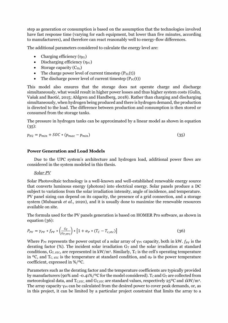
step as generation or consumption is based on the assumption that the technologies involved
have fast response time (varying for each equipment, but lower than five minutes, according
to manufacturers), and therefore can react reasonably well to energy-flow differences.
The additional parameters considered to calculate the energy level are:
• Charging efficiency (ηEL)
• Discharging efficiency (ηFC)
• Storage capacity (CH2)
• The charge power level of current timestep (PEL(t))
• The discharge power level of current timestep (PFC(t))
This model also ensures that the storage does not operate charge and discharge
simultaneously, what would result in higher power losses and thus higher system costs (Gulin,
Vašak and Baotić, 2015; Ahlgren and Handberg, 2018). Rather than charging and discharging
simultaneously, when hydrogen being produced and there is hydrogen demand, the production
is directed to the load. The difference between production and consumption is then stored or
consumed from the storage tanks.
The pressure in hydrogen tanks can be approximated by a linear model as shown in equation
(35):
𝑝𝐻2 = 𝑝𝑚𝑖𝑛 + 𝑆𝑂𝐶 ∗ (𝑝𝑚𝑎𝑥 − 𝑝𝑚𝑖𝑛) (35)
Power Generation and Load Models
Due to the UPC system’s architecture and hydrogen load, additional power flows are
considered in the system modeled in this thesis.
Solar PV
Solar Photovoltaic technology is a well-known and well-established renewable energy source
that converts luminous energy (photons) into electrical energy. Solar panels produce a DC
subject to variations from the solar irradiation intensity, angle of incidence, and temperature.
PV panel sizing can depend on its capacity, the presence of a grid connection, and a storage
system (Mubaarak et al., 2020), and it is usually done to maximize the renewable resources
available on site.
The formula used for the PV panels generation is based on HOMER Pro software, as shown in
equation (36):
𝑃𝑃𝑉 = 𝛾𝑃𝑉 ∗ 𝑓𝑃𝑉 ∗ (𝐺𝑇
𝐺𝑇,𝑆𝑇𝐶) ∗ [1 + 𝛼𝑃 ∗ (𝑇𝐶 − 𝑇𝑐,𝑠𝑡𝑐)] (36)
Where PPV represents the power output of a solar array of γPV capacity, both in kW. 𝑓𝑃𝑉 is the
derating factor (%). The incident solar irradiation GT and the solar irradiation at standard
conditions, GT, STC, are represented in kW/m2. Similarly, TC is the cell’s operating temperature
in ºC, and TC, STC is the temperature at standard condition, and αP is the power temperature
coefficient, expressed in %/ºC.
Parameters such as the derating factor and the temperature coefficients are typically provided
by manufacturers (90% and -0.41%/ºC for the model considered). TC and GT are collected from
meteorological data, and TC,STC, and GT,STC are standard values, respectively 25ºC and 1kW/m2.
The array capacity γPV can be calculated from the desired power to cover peak demands, or, as
in this project, it can be limited by a particular project constraint that limits the array to a

specific maximum power. Based on the area provided by the university, the capacity considered
is 12kW.
Compressor Power
As discussed in chapter 2.3, hydrogen compression can require significant energy inputs to
the electrical load. In this model, a mechanical type of compressor unit is considered. The
specific work of a compressor at an ideal condition can be described by equation (37):
𝐿𝑖𝑠,𝑐 =𝑘
𝑘−1∗ 𝑅𝐻2 ∗ 𝑇𝑖𝑛 ∗ [
𝑝𝑜𝑢𝑡
𝑝𝑖𝑛
𝑘
𝑘−1 − 1] (37)
Where k is 1.4 and represents the ratio of hydrogen gas’ specific heats (cp and cv), and RH2
(4.12 kJ/kg K) represents the hydrogen gas constant. Tin (K) is the temperature at the
compressor’s inlet -considered the same ambient temperature. The pressures pout and pin are
the pressures at the compressor’s exit, considered the same as the hydrogen tanks, and into
the compressor, considered the same as exiting the electrolyzer and a buffer tank.
Yellow Hydrogen Electrical Load
As UPC’s hydrogen demand is significantly higher than its electrical load and its renewable
power generation, grid electricity is used to guarantee hydrogen storage is always at a level that
can supply the lab’s activities. The electrical consumption needed for this hydrogen production
is calculated similarly to the electrolyzer power consumption described in equation (38), in an
opposing direction:
𝑃𝑦𝐸𝐿 = 𝐻𝐿𝑜𝑎𝑑 ∗𝑃𝑁𝑜𝑚𝑖𝑛𝑎𝑙
𝜂𝐸𝐿 (38)
Managing storage of different hydrogen colors
A particular characteristic of the UPC’s showroom is the different scales and hydrogen load
profiles for feedstock and electricity. As the laboratory seeks to maintain its electric
consumption as independent from the grid as possible, it needs to differentiate the storage
used for green and yellow hydrogen, as represented in Figure 24.
Green hydrogen consumed in the fuel cells would provide clean power to the laboratory’s
electric load accounting for daily and monthly seasonal effects. On the other hand, the
consumption of yellow hydrogen produced from the grid would implicate significantly higher
losses during electrolysis, compression, and storage, thus having a higher environmental and
economic impact.
Figure 24. Illustration of the green and yellow hydrogen division
Two different storage management strategies are suggested to guarantee that the lab’s
electricity is always supplied by the lowest carbon-emitting source and the most economical
option. In practice, hydrogen gas has no differentiation between its molecules, and therefore
these storage strategies work on estimations of production and consumption instead of actual
measures of storage level. In cases with a highly modularized storage system, exclusive storage
can be assigned for hydrogen produced from renewable energy, requiring adaptations on the
pipelines and the EMS system.
For green hydrogen storage, two lower-limit levels are set. Instead of a minimum pressure
limit, relative zero is set as the amount of green hydrogen at the beginning of the simulation.
Fuel cells are only supplied by green hydrogen, and a second limit is set for the lab’s test
stations, as represented in Figure 25.
Figure 25. The decision process for consuming green hydrogen.
No upper limit is set for green hydrogen, and 80% of the total capacity is initially set for yellow
hydrogen. The sum of both storages has an upper limit equal to the storage installed capacity.
The decision-making process used in the model follows the simplified explanation below and
is illustrated in Figure 26.
1. Solar PV energy will be used to fulfill the load directly whenever available.
2. When solar energy exceeds electrical demand, it is used for hydrogen production.
3. If electrolyzers are already activated by excess PV energy, AND grid prices are below a
defined threshold, AND SOCH is below 30%, produce more hydrogen. For this
simulation, the price threshold of 0.18 €/kWh is used.
4. When no solar energy is available and hydrogen storage is low, the grid is used
considering:
a. If storage is above a critical level, hydrogen is produced at lower grid fares.
b. If storage is below a critical level, hydrogen is produced at any time.

Figure 26. SOCH charge point conditions.
As for the scenario’s economic feasibility, capital and operational expenditures will be taken
into consideration, as described below:
• Capital Expenditure (CAPEX) Equipment acquisition
▪ Electrolyzers
▪ Compressors
▪ Storage tanks
▪ Fuel Cells
▪ Power electronics
▪ Other Installation (cabinets, piping, cabling, and others)
• Operational Expenditure (OPEX)
Grid-Electricity cost
Maintenance costs
The building will provide solar panels, and therefore are not included in this analysis.
The environmental impact in this scenario will come from grid-related emissions. Barcelona’s
grid emissions are monitored by Spanish operator Red Eléctrica de España and change
according to the share of renewables active in the grid.

5 SIMULATION RESULTS
In this section, the simulation results of the two scenarios described in section 6 are shown. A
logistic approach is used for the base case to resupply grey hydrogen, and an EMS approach is
suggested. After an initial simulation with the specifications laid out by UPC’s engineering
team, changes in parameters were simulated to understand their impact on the overall system.
The lab’s expected hydrogen and electrical load were kept the same for all simulations, as well
as its renewable energy resources.
5.1 BASE CASE - GREY HYDROGEN PURCHASING The base case modeling described in section 4.1.1 was applied for each project phase's expected
hydrogen and electrical load. The results shown in this chapter represent the system fully
operational at phase three and maximum hydrogen load.
5.1.1 Storage Levels
Figure 27 exhibits a closer look into the storage profile for a typical July month. On a typical
week, the steep decrease in storage can be seen during office hours and a slight decrease during
nighttime and weekends. The weekly average storage is indicated as a blue line for a better
understanding of the lab’s yearly storage profile, as shown in Figure 28.
Figure 27. Profile of grey hydrogen consumption for a typical summer month.
While the average storage remains relatively stable within a month, the varying profiles of
hydrogen load and supply chain constraints can result in some false seasonality, which can
implicate cut-off and OOH occurrences when storage reaches the values of a hundred and zero
kg, respectively. The storage capacity’s impact on system reliability was evaluated for similar
supply chain parameters and is shown in Table 8.

Figure 28. Instantaneous hydrogen storage and weekly moving average for a grey hydrogen purchasing scenario.
Table 8. Impact of storage size on OOH and Cut Off indicators for a retail hydrogen scenario.
Max Storage (kg) OOH Cut-Off (kg/year) HNS (kg/year)
25 12% 113.30 370.7
35 1% 63.44 38.1
50 0 25.26 0
75 0 31.53 0
100 0 24.75 0
5.1.2 Reliability
As the safety storage level chosen is relatively high, the base case did not reach SOHs low
enough to disrupt the laboratory’s activities. This indicates that smaller installed capacities
could be selected, reducing the scenario’s costs.
On the other hand, some hydrogen was lost as a cut-off in the replacement of bottles, which
could be more frequent with smaller capacities that require a more complex storage
calculation. Hydrogen cut-off is a problem to be avoided, where significant amounts of
hydrogen can be lost every time bottles are replaced. For the simulated scenario, 1.05% of the
lab’s hydrogen demand is wasted, as shows Figure 29.

Figure 29. Hydrogen consumed and hydrogen losses on a retail scenario.
5.1.3 Economics
Figure 30 shows the estimated expenses with hydrogen purchasing to maintain the
laboratory’s fuel cell activities and costs with electricity purchased from the grid. A somewhat
regular supply of hydrogen can be seen for the lab, which could open the way to negotiate better
prices with suppliers.
Figure 30. Base case weekly costs with hydrogen and electricity.
Over a year, the expenses related to the base case scenario are grey hydrogen purchases, grid
electricity, and the person-hour cost of replacing the storage at each delivery. No installation
or initial investment is considered, and the cost with hydrogen is set as the same after the third

year when all laboratory testing stations are installed, and hydrogen consumption is at its
maximum.
Figure 31 shows the cost projection over time, and Figure 32 shows the ACS estimated for this
scenario.
Figure 31. Base case costs, with grey hydrogen retail
We can see that the impact of bottle rental is significant in the base case scenario. This is a
characteristic of the retail hydrogen business model and, according to the current supplier, it
is impossible for consumers to own the bottles and refill only the hydrogen gas consumed for
such a small hydrogen consumption.
Figure 32 shows the evolution of total cost, and the effect of time over the years. The Anualized
Cost of System for the base case was found to be 418.23 thousand Euros over a period of 20
years. the Levelized Cost of Hydrogen (LCOH) over the 20 years was 9.23€/kg, of which
approximately 63% of this impact comes from fixed costs with bottle rentals.
Figure 32. Cost progression over different time horizons for a hydrogen retail scenario.

5.1.4 Sustainability and Environment
Figure 33 shows the estimated emissions for a hydrogen retail scenario. Grey hydrogen
emissions are those resulting from the steam reforming of natural gas, delivery emissions are
those resulting from the transportation of hydrogen via road transportation and grid emissions
are the emissions resulting from the electrical load.
Besides weeks 31 to 35, when most team members are on vacation, emissions remain
reasonably stable, with minor changes following the defined hydrogen load profile. SMR is the
primary source of CO2 emissions, amounting to approximately 22.6 tons of CO2 in a year, using
an estimative of 9.3 kg of CO2 per kg H2 (Rapier, 2020).
Figure 33. Estimated emissions for a retail hydrogen scenario.
5.2 HYBRID SOLAR-PV, GRID, AND HYDROGEN MICROGRID
As for the base case, the microgrid case simulation was carried out considering the different
installation phases, as described in section 3.6.1. The resulting simulations described in this
section represent the simulation at phase three and hence after the installation is complete.
5.2.1 Storage Levels
Figure 34 shows the instantaneous, daily, and weekly storage profiles.

Figure 34. Hydrogen storage profile for UPC's microgrid
The first notable aspect of the storage level profile is the reliability of the EMS system
implemented. During the entire simulation the system did not fall under dangerously low
levels, neither did it reach the storage’s maximum capacity, which could result in eventual
renewable energy curtailments. While the storage may seem oversized, the installed capacity
is enough for only two days of hydrogen consumption in the lab. Having relatively stable two-
days storage levels can give researchers the freedom to schedule intensive tests a couple of days
in advance, which could be beneficial to the lab’s daily operations and profitability.
Moreover, the storage level is understandably higher and more stable during the laboratory
vacations and holidays (mid-August to September and December-January) due to the reduced
hydrogen feedstock demand.
A robust daily variation can be seen, resulting from a combination of factors. First, hydrogen
demand peaks during work hours, with a substantial consumption when grid prices are high.
At those moments, only excess solar energy is converted into green hydrogen, while the fuel
cells remain offline. Prices are also lower later in the day, between 14 and 18h, which could be
an additional schedule to run the electrolyzers. The refueling behavior could change with
dynamic grid prices or previously agreed on prices, changing the optimization strategy to
reduce electricity expenses. Figure 35 visualizes the daily variations.

Figure 35. Hydrogen microgrid storage profile over a spring month
5.2.2 Reliability
Figure 36. State of charge of the microgrid's hydrogen storage
While daily SOH levels do not reach zero, the lowest level reached is 26.65% of storage by late
February. It is interesting to remember that the lower limit for regular charging was set at 30%
SOCH, at which the electrolyzers begin to recharge the storage when prices are low. This limit
was only reached a few times, while most times, the electrolyzers operated with low fares when
the solar panels already activated them. A critical SOCH of 10% was never noticed, further
proving the system capacity can recover the storage on the assigned schedule times.
It is visible that the microgrid can achieve satisfying reliability for hydrogen supply, which can
be attributed to the hydrogen generated being mostly yellow, produced with grid electricity
that is always readily available for consumption (Mubaarak et al., 2020). The cut-off indicator
did not show any occurrences during the entire simulation, as a higher limit was set for yellow
hydrogen, and green hydrogen production was not enough to surpass demand.

5.2.3 Equipment performance
Rates of Utilization
Figure 37. Electrolyzer and Fuel Cell rates of utilization and the average level of green hydrogen storage
The weekly rates of utilization for the fuel cells and electrolyzers are shown in Figure 37 and
Figure 38.
In Figure 37, the system is considered idle when hydrogen storage is sufficiently high not to
have electrolyzers activated and when there is no available green hydrogen to fuel the fuel cells,
which only happened on the first days of the simulation. Electrolyzer utilization rates increase
during summer, with longer hours of sunlight, and stronger irradiation, reducing the need for
power production from the fuel cells.
As expected, electrolyzers work predominantly during the day, when excess solar energy is
available, and at moments where grid rates are lower. In Figure 38, the intensity of positive
values represents the percentage of electrolyzer capacity in use. Bright yellow markings
represent electrolyzers working at total capacity, while -1 to 0 represent the rate of utilization
of the fuel cells. For the sake of better visualization, fuel cell values were normalized at their
peak power production of close to 3kW. Most of the time, however, the fuel cell system ran
below that value.
Fuel cells utilization rate is typically higher in late evenings, represented by blue dots in Figure
38. in moments where storage levels are high enough not to need the electrolyzer’s
intervention, such as during the night and early morning, fuel cells work fulfilling the small
electrical load of appliances running overnight. Figure 39 zoom in a typical winter and summer
week, showing the average hydrogen storage level, and the fuel cell and electrolyzer’s rates of
utilization.

Figure 38. Electrolyzer and Fuel Cell utilization rates
Figure 39. Electrolyzer and Fuel Cell utilization rates into typical winter and summer weeks

Compressor
While most of the electricity demand comes from laboratory appliances and electronics, the
compressor’s electrical consumption is significant, amounting to nearly 32% of the overall
electricity demand Figure 40. Logically, as hydrogen production increases in peak demand
months, the compressor’s usage and electric demand increase as hydrogen production
increases. Still, the fuel cells were largely sufficient to cover the power needed for both
compressor and laboratory load.
Figure 40. Electricity demand by source
Electrolyzer utilization
Figure 41 indicates that the electrolysis system worked mostly with grid electricity to keep up
with the substantial hydrogen load for the lab’s test stations. When university activities are
usually slower between August and September (weeks 32 to 35), renewable hydrogen
production and share are highest, as green hydrogen gross production naturally follows the
increase in solar irradiance.

Figure 41. Electrolyzer energy consumption by energy source
5.2.4 Sustainability and Environment
Renewable Electricity and Green Hydrogen
Figure 42 and Figure 43 and show in green the share of the total electricity supplied by
renewable energy sources, either directly from solar panels or indirectly via the fuel cells.
Renewable energy electricity is prevalent all year round, peaking at 95.56% in weeks 21 when
solar energy is high and the lab has a reduced hydrogen demand. Daily, renewable electricity
can reach 100% on sunny days and when fuel cells work at night based on green hydrogen
consumption (?), as shown in Figure 44. As a constraint was set for the electrolyzer and the

fuel cell not to work simultaneously, complementary battery storage could improve the overall
renewable electricity share (Ahlgren and Handberg, 2018).
Figure 42. Weekly Renewable Electricity Share.
Figure 43. Weekly Renewable Hydrogen Share.

Figure 44. Renewable electricity and hydrogen share daily
However, the share of green hydrogen supplied to the lab is close to zero during the entire
simulation, reaching 5,64% at its peak in Mid-August. The overall low share is due to two main
reasons: the lab’s hydrogen load being significantly higher than what the available solar panel
capacity can provide and the prioritization of green hydrogen to the showroom’s fuel cells, to
avoid unnecessary losses. Peak renewable hydrogen feedstock is achieved when most lab
activities are on vacation, while solar PV generation is high.
Figure 45. Source of electricity supplied to the lab in Wh

Figure 46. Source of electricity supplied to the lab as a percentage of demand
The profile of electricity supply to the laboratory’s electrical needs and the compressor are
shown in Figure 45 and Figure 46. Most of the electricity is supplied directly by the solar panels,
which increases with solar irradiation towards summer. Both PV electricity generation and
green hydrogen generation increase over the summer, when the system achieves 30.58% of
hydrogen generation from renewable energy, see Figure 47.
Figure 47. Green and Yellow hydrogen production shares
CO2 emissions from this case are related to electricity consumption from the grid, see Figure
48. Therefore, the lab’s emissions (in green) are higher in weeks, where the Spanish grid’s
carbon intensity is higher (in yellow). On a quarter-hourly basis, emissions are lower when

renewable energy generation is higher, which coincides with lower grid prices. Emissions are
also lower in months where the lab staff has a reduced workload. The total emissions were
estimated to be around 19 tons of CO2 per year at Spain’s current electricity mix.
Figure 48. Weekly CO2 emissions related to the microgrid.
5.2.5 Economics
As for the base case, investment, replacement, operation, and maintenance costs were
projected over 20 years.
Some important considerations:
• Equipment prices were obtained from system integrators consulted during this work.
• As both the electrolyzers and fuel cells systems were sized to be highly modular in the
actual project, their replacement cost is considered half of the initial investment,
simulating the replacement of half the modules.
• The building supplies clean water at no cost to the lab, so it was not considered in this
analysis.
• Labor cost is considered when pieces of equipment are installed, for example, in each
project phase and replacements.
Figure 49 groups in CAPEX all the investment costs necessary in the installation dates, in
CAPEX replacements, the costs to replace electrolyzer and fuel cell modules, including labor,
and expenditures with maintenance and electricity. Figure 50 breaks down costs in detail by
each component for in-depth analysis.

Figure 49. Overall cost structure over the years for the main case
Figure 50 Detailed cost structure over the years for the hydrogen microgrid.

Figure 51. Breakdown of investment costs by component
As for the investment necessary, Figure 51 exhibits the cost share of each component installed,
and Figure 52 divides them in each phase. It is visible that considerable impacts on cost come
from the hydrogen compressor and electrolyzers, which is coherent with other studies (Yang
et al., 2008; Ahlgren and Handberg, 2018; Sdanghi et al., 2019; Nastasi et al., 2021;
Christensen, no date). Even with one of the most competitive electrolyzers in the market, the
technology is still expensive, representing 18.7% of total investment and 28.9% of equipment
investment.
Hydrogen compression also significantly impacts cost, amounting to 30.53% of total
investment and 46.5% of equipment investment. Compression costs increase significantly with
the choice of storage pressure, as for the compression energy consumption (Sdanghi et al.,
2019). System integrators contacted recommend adding buffer tanks between the electrolyzers
and compressors to mitigate this high cost. This addition can significantly reduce the required
compression installed capacity.
Figure 52. Breakdown of investment costs by component and phase

To better understand the impact of the hydrogen compression technology chosen and the use
of a buffer tank, a preliminary cost comparison was carried out between five scenarios altering
the compressor technology and installed capacity, as represented in Table 9. An upcoming
Electrochemical Compression () technology was compared to a conventional metal diaphragm
compressor.
Table 9. Cost scenarios for different hydrogen compression technologies and the use of a buffer tank.
Scenarios Compressor Price
Compressor capacity
Modules Total Capacity
Total Compression Cost
Source
Expected average + EC €107,000.00 10kg/day 2 20kg/day €214,000.00 (HyET, 2021)
Total with EC + Buffer €107,000.00 10kg/day 1 10kg/day €107,000.00 (HyET, 2021)
Expected average + Mechanical Compressor without buffer
€17,938.28 1.1kg/day 7 7.7kg/day €125,567.96 (SERA, 2021)
Expected average + Mechanical Compressor WITH buffer
€17,938.28 1.1kg/day 3 3.3kg/day €53,814.84 (SERA, 2021)
Figure 53 exhibits the cost progression of each phase, as well as the total cost. According to the
market data collected, installing a buffer tank can reduce system costs up to 47% for a
mechanical compressor and 27% for EC. Still, even if more expensive at first sight, EC can be
more economical and add several advantages to the system, such as hydrogen filtering,
adaptation to variable loads, and higher compression pressures (HyET, 2021).
Figure 53. Cost comparison of EC and Mechanical compression technologies with and without a buffer tank.
The evolution of ACS for the hydrogen microgrid case is shown in Figure 54.

Figure 54. Cost evolution and ACS of the hydrogen microgrid case.
6 RESULT COMPARISON AND ANALYSIS
This chapter intends to compare both scenarios by their storage levels, reliability, performance,
sustainability, and economics. The chapter describes whether UPC’s microgrid can be
competitive with their current grey hydrogen retail model, or at least not impeditive in the
pursuit of a sustainable hydrogen supply
6.1 STORAGE CAPACITY AND STORAGE LEVELS On a retail hydrogen scenario (base case), larger hydrogen storage is required to mitigate
supply chain effects, which results in higher costs from bottle rental. Additionally, storing large
quantities of such highly explosive gas can stumble on footprint and safety constraints at a
commercial building like UPC’s (Grigoriev et al., 2009). Additionally, even with a large storage
capacity, the number of deliveries in a year would be overwhelming to UPC’s technicians, who,
according to them, would need to dedicate half an hour to one hour of labor for the replacement
of hydrogen bottles, which also increases the risk of accidents by manual intervention.
On the other hand, the hydrogen microgrid and the EMS model could maintain perfect
reliability indicators during the entire simulation time. Such a system can increase the
laboratory's structure and confidence to carry out more extensive research projects, probably
increasing the laboratory’s income over the years.
6.2 RELIABILITY The base case simulated in this thesis relies on some fundamental assumptions particular to
the Barcelona region and is, to a certain degree, already reality for UPC’s hydrogen team. A
well-established hydrogen supply chain and a natural gas network result in reliable lead times,
which in turn help the laboratory’s team to plan their testing schedules, thus minimizing the
chances of hydrogen. In such a scenario, it is reasonable to assume that even intensive fuel cell
testing, such as for heavy-duty transportation cycles, can be scheduled in advance without the
risk of running out of fuel. Similarly, Cut Off hydrogen can be minimized with proper demand
planning.
As this scenario considers a grid connection as the sole source of electricity for the lab’s power
demand, LPSP can be considered zero.

For the main case, however, reliability seems flawless. As demands grow over the years, this
scenario also indicates to be more reliable, as the EMS could be further improved. The system’s
modularity could also favor future expansions without more considerable investment costs,
mitigating eventual decreases in reliability caused by increased hydrogen and electricity
demand.
6.3 SUSTAINABILITY Although third scope emissions were not considered, the microgrid case indicates to be
undoubtedly superior on environmental aspects. As long as the retail market supplies
predominantly grey hydrogen, emissions will be higher than from a microgrid. Additional
emissions from transportation and methane leakage are also inevitable and can amount to a
significant carbon footprint. While emissions from the base case are estimated to be higher
than the microgrid’s, one could argue they are not significant enough to justify the investment
in a complex system that can account for third-scope emissions. However, it is essential to note
that the chosen control strategy focused on reducing grid electricity prices, not considering
punctual emission intensities. Lower emission rates can be achieved by adding an
environmental objective function to the control strategy. Securing a power purchasing
agreement for cheaper local renewable electricity or installing more solar panels would reduce
both the cost and emissions.
Moreover, Spain is becoming a European leader in moving towards renewable energies,
increasing its investments in solar and wind energy (McKinsey, 2020). Spanish grid emissions
are expected to keep decreasing, further reducing emissions related to yellow hydrogen
production. The Spanish grid carbon intensity is forecasted to drop below 100 grams per
kilowatt-hour, which would result in 10.81t of CO2 emissions per year, a 43% decrease under
the same operating conditions.
6.4 ECONOMICS
As mentioned previously, the proposed hydrogen microgrid’s ACS is 66% higher than the base
case, a significantly more costly path, at the considered hydrogen costs and interest rates, as
shown in Figure 55. This result is understandable, as the base case scenario does not involve
initial investments and hydrogen technologies are still moving towards market acceptance
(Hydrogen Council, 2020). On an operational basis, O&M costs were slightly higher for the
microgrid at the grid prices considered. A future reduction in electricity prices could also
change the dynamics of this result, something that is already extensively forecasted by industry
(Hydrogen Council, 2020).

Figure 55. ACS cost comparison
An analysis of the effect of grey hydrogen cost on the base case’s ACS shows that UPC’s
microgrid can be competitive with the base case for retail prices above 15 euros per kilogram
of hydrogen in 15 years, as shows Figure 56. This number seems unrealistic compared to the
low prices of grey hydrogen today, but not too far from hydrogen prices charged by retailers to
small consumers such as research centers. Still, if the natural gas supply is available at the
university, a more direct, on-demand, grey hydrogen production capacity investment could be
made to supply the lab at much lower prices. At the studied timeframe of 20 years, the
microgrid case amounts to approximately €589 thousand euros, while a scenario of retail
hydrogen at 15€/kg would amount to €645 thousand euros. Accounting with the capex cost
reduction forecasted by industry, an ACS of €403 thousand euros could be achieved for the
hydrogen microgrid, slightly more competitive than a 6€/kg of hydrogen scenario.

Figure 56. ACS evolution for different retail hydrogen prices
7 SYNTHESIS AND DISCUSSION
A summary of the results is provided in this chapter, along with Table 10 comparing the results
of both scenarios. While the hydrogen microgrid causes initially a significantly higher cost to
UPC, its ecological and technical advantages might outweigh the economical drawbacks. The
proposed microgrid excels compared to the grey-hydrogen scenario on parameters such as
reliability, sustainability, and social-political influence, while also having better future
perspectives with the forecasted reduction of electricity and equipment cost.
First, it was proven that the storage capacity necessary for the base case scenario was more
prominent than the storage capacity required in the microgrid scenario. This result can be
related primarily to the supply chain constraints and secondly to the need for a more intelligent
demand planning algorithm to guarantee reliable hydrogen supply to the lab in the grey
hydrogen scenario. It was shown that storage capacity needed to be increased to avoid eventual
mismatches in hydrogen supply for the laboratory's activities, increasing the costs with bottle
rentals significantly.
The proposed hydrogen microgrid seems to be preferable on the reliability sphere, because of
its more stable storage levels, responding rapidly to peak demand and peak generation. Having
spare storage levels is especially important for this project, as it gives the laboratory more
flexibility to run unscheduled intensive fuel cell tests that would significantly increase
hydrogen demand. This reliability can be partially attributed to the grid connection that can
provide electricity not just directly to the laboratory but also to the electrolyzers.
Furthermore, as proven by several studies in literature, the methodology applied in this thesis
shows that an EMS has a substantial impact on the system’s storage level, energy consumption,
system reliability, and economics. Depending on the objectives, different parameters of the
microgrid system could be adjusted: further improve renewable energy share, avoid
0
100
200
300
400
500
600
700
800
0 1 2 3 4 5 6 7 8 9 10 11 12 13 14 15 16 17 18 19
AC
S (
€)
Th
ou
san
ds
Years
Sum of 4€ /kg - ACS
Sum of 6€ /kg - ACS
Sum of 10€ /kg - ACS
Sum of 12€ /kg - ACS
Sum of 15€ /kg - ACS
Sum of 17€ /kg - ACS
Sum of Competitive CAPEXACS
Sum of ACS- UPC

curtailments, reduce system capacity, and further reduce costs (Garcia, Dufo-López and
Bernal-Agustín, 2019).
This study also demonstrates that we are not that far from yellow as well as green hydrogen
being competitive with grey hydrogen, , something already expected by key players within
industry (Hydrogen Council, 2020). This opens a discussion to entirely new possibilities of
using hydrogen as feedstock in industry, in applications where high hydrogen demands are
needed, but renewable energy generation is limited or unavailable on site.
However, the base case chosen for comparison was more economical than the hydrogen grid
modeled, which is in line with recent studies carried out by leading consultancy firms and
governmental agencies. Today, it is a fact that grey hydrogen costs are significantly lower than
green hydrogen due to the low price of natural gas and the expensive cost of electricity in many
regions. However, this is set to change in the future. Hydrogen is not only estimated to become
more competitive in the coming decades, but it is also believed to be an essential piece of
solving the climate change puzzle. For example, in the European continent, the climate target
of reaching net-zero emissions by 2050 is believed to be impossible without green and blue
hydrogen (McKinsey, 2020).
Furthermore, the entire energy system will be influenced by the upcoming development of the
hydrogen economy. Carbon emitting prices are hitting consecutive record highs as the world
moves towards cleaner technologies, which will undoubtedly increase the cost of pollution
emitters, such as fossil-fueled electricity and steam methane reforming. The impact of climate
concern goes even further, as carbon pricing moves towards a new paradigm with the advance
of the hydrogen economy. A recent study by BNP Paribas shows that future carbon pricing will
shift from balancing the cost of making natural gas competitive with coal energy generation,
towards the cost difference between the generation of gray and green hydrogen (Lewis, 2020a,
2020b).
Finally, this thesis can be seen as a pilot project for larger as well as smaller grid-connected
hydrogen generation systems and an inspiration to the shift away from grey hydrogen and
fossil-fueled energy to cleaner alternatives, even if not completely green. The model and the
EMS system can be implemented for larger capacities and easily tailored for specific
applications, instigating future work developing the hydrogen economy.
7.1 SUMMARY This chapter presents a summary of the results achieved in this thesis.
• A grid-connected hydrogen production microgrid was designed with solar electricity as renewable energy support, AEM electrolyzers, mechanical compressors, pressurized
storage tanks, and PEM fuel cells.
• An EMS was suggested to maintain satisfactory reliability levels for hydrogen
production, also achieving reliable electricity supply.
• A techno-economic model was also created to assess the system’s viability and compare
different equipment configurations, as well as to compare with a grey hydrogen case.
• The suggested microgrid was found to have higher investment costs, but better
technical and ecological performance over the year than a retail hydrogen scenario.
• The addition of buffer tanks strongly reduces system cost, bringing the microgrid ACS close to that of a retail hydrogen scenario.
• It was found that the proposed system can be competitive on a 15-year horizon at today’s costs against a retail price of 15€/kg of hydrogen.

• It was also found that for the hydrogen system to be competitive with a 10€/kg of
hydrogen scenario, a 69% CAPEX reduction is needed, something not far from what is
forecasted by industry.
Table 10 exhibits a qualitative summary of each performance indicator analyzed in this thesis,
showing that the advantages of a hydrogen microgrid go beyond its more expensive economics.
Table 10. Qualitative summary of the scenarios compared.
Parameter Base Case Hydrogen Micro-grid Storage Capacity - ++ Reliability + +++ Environment - - +++ Economics ++ - Future Perspectives - - +++

8 CONCLUSIONS
This thesis study was written in parallel to UPC’s project timeline. During the project, the thesis
methodology was applied in parallel to the showroom’s planning and engineering phases,
where work such as research of components, contact with suppliers and clients, along with
system sizing and project quotations were carried out to collect data both for the project and
for this thesis. This master thesis also presented a modeling approach for mixed green and
yellow hydrogen microgrids, simulation, and a first look into the optimization of UPC’s
microgrid.
The questions listed in Section Error! Reference source not found. were addressed as
follows:
• What are the state-of-the-art technologies available in the market, and how would they affect the technical and economic feasibility of a micro-grid?
It was found that AEM electrolyzers, mechanical compressors, pressurized storage tanks, and
PEM fuel cells were the optimal technologies for both price and performance, being also easily
accessible in the European market. These technologies show fast response times which gives
the microgrid more flexibility to switch modes according to the laboratory’s dynamic loads.
• How to design a hydrogen micro-grid for best techno-economic performance?
For UPC’s hydrogen needs, a grid-connection is vital, and it will be the main source of energy
for hydrogen production. The granted area for solar panels is enough to supply electricity
directly to electrical loads when solar resource is available, and a small amount of green
hydrogen. It was found that for a safe operation in the hydrogen-consuming laboratory, a
pressurized storage capacity of close to two days of average consumption was necessary, given
that the electrolyzer capacity and the grid connection can guarantee the system does not fall
under critical levels. To achieve pressures of 400 bar and reduce the space taken by cylinders,
a compressor is added to the system, further increasing electricity consumption. A buffer tank
was also found to significantly reduce the system’s CAPEX, as it results in less compression
required. All the technologies assessed are forecasted to improve in the coming years, creating
good perspectives for the feasibility of similar grids. Finally, for green electricity production,
when solar energy is not available, green hydrogen is used in PEM fuel cells that were oversized
on purpose to allow future expansion of lab activities.
• How can the designed energy management system make UPC’s hydrogen microgrid more competitive with grey hydrogen?
The designed EMS has a significant impact on the system’s reliability and environmental
impact. A strategy to manage the storage of different hydrogen colors prevents unnecessary
thermodynamic losses and reduces operation costs, thus improving the microgrid’s ACS. The
EMS was also set to produce hydrogen only at reduced grid prices, which in the future can be
further improved if grid tariffs get lower with time.
The EMS system proposed proved to be a reliable controlling strategy for the modeled
microgrid. Furthermore, the results of the techno-economic analysis resonate with current
market estimations for grey and green hydrogen costs, while the projected electricity and
hydrogen costs reductions indicate a shift in future towards green hydrogen project economic
viability.

9 REFERENCES
Abbaspour, A., Parsa, N. and Sadeghi, M. (2014) ‘A New Feedback Linearization-NSGA-II based Control Design for PEM Fuel Cell’, International Journal of Computer Applications, 97, pp. 25–32. doi:10.5120/17044-7354.
Ahlgren, P. and Handberg, E. (2018) ‘System performance analysis of an isolated microgrid with renewable energy sources and a battery and hydrogen storage system - An evaluation of different storage system configurations’, CODEN:LUTEDX/TEIE [Preprint]. Available at: http://lup.lub.lu.se/student-papers/record/8937880 (Accessed: 26 July 2021).
Andreasson, M. et al. (2013) ‘Distributed vs. centralized power systems frequency control’, in 2013 European Control Conference (ECC). 2013 European Control Conference (ECC), pp. 3524–3529. doi:10.23919/ECC.2013.6669721.
Andrew Beattie (2021) How to Calculate Return on Investment (ROI), Investopedia. Available at: https://www.investopedia.com/articles/basics/10/guide-to-calculating-roi.asp (Accessed: 30 July 2021).
Barthelemy, H., Weber, M. and Barbier, F. (2017) ‘Hydrogen storage: Recent improvements and industrial perspectives’, International Journal of Hydrogen Energy, 42(11), pp. 7254–7262. doi:10.1016/j.ijhydene.2016.03.178.
Bizon, N., Oproescu, M. and Raceanu, M. (2015) ‘Efficient energy control strategies for a Standalone Renewable/Fuel Cell Hybrid Power Source’, Energy Conversion and Management, 90, pp. 93–110. doi:10.1016/j.enconman.2014.11.002.
Brka, A., Al-Abdeli, Y.M. and Kothapalli, G. (2015) ‘The interplay between renewables penetration, costing and emissions in the sizing of stand-alone hydrogen systems’, International Journal of Hydrogen Energy, 40(1), pp. 125–135. doi:10.1016/j.ijhydene.2014.10.132.
Byrne, R.H. et al. (2018) ‘Energy Management and Optimization Methods for Grid Energy Storage Systems’, IEEE Access, 6, pp. 13231–13260. doi:10.1109/ACCESS.2017.2741578.
Cau, G. et al. (2014) ‘Energy management strategy based on short-term generation scheduling for a renewable microgrid using a hydrogen storage system’, Energy Conversion and Management, 87, pp. 820–831. doi:10.1016/j.enconman.2014.07.078.
Christensen, A. (no date) ‘Assessment of Hydrogen Production Costs from Electrolysis: United States and Europe’, p. 73.
Cipriani, G. et al. (2014) ‘Perspective on hydrogen energy carrier and its automotive applications’, International Journal of Hydrogen Energy, 39(16), pp. 8482–8494. doi:10.1016/j.ijhydene.2014.03.174.
Conti, S. et al. (2012) ‘Optimal Dispatching of Distributed Generators and Storage Systems for MV Islanded Microgrids’, IEEE Transactions on Power Delivery, 27(3), pp. 1243–1251. doi:10.1109/TPWRD.2012.2194514.
Cornell, A. (2020) ‘Hydrogen production by electrolysis’.
DOE (2016) ‘Comparison of Fuel Cell Technologies’, p. 1.

Eriksson, E.L.V. and Gray, E.MacA. (2017) ‘Optimization and integration of hybrid renewable energy hydrogen fuel cell energy systems – A critical review’, Applied Energy, 202, pp. 348–364. doi:10.1016/j.apenergy.2017.03.132.
European Union, P.O. of the (2020) ‘A hydrogen strategy for a climate-neutral Europe’. Publications Office of the European Union. Available at: http://op.europa.eu/en/publication-detail/-/publication/5602f358-c136-11ea-b3a4-01aa75ed71a1/language-en (Accessed: 19 August 2021).
Garcia, Y., Dufo-López, R. and Bernal-Agustín, J. (2019) ‘Energy Management in Microgrids with Renewable Energy Sources: A Literature Review’, Applied Sciences, 9, p. 3854. doi:10.3390/app9183854.
Gou, B., Na, W. and Diong, B. (2016) Fuel Cells: Dynamic Modeling and Control with Power Electronics Applications, Second Edition. CRC Press.
Grigoriev, S.A. et al. (2009) ‘Hydrogen safety aspects related to high-pressure polymer electrolyte membrane water electrolysis’, International Journal of Hydrogen Energy, 34(14), pp. 5986–5991. doi:10.1016/j.ijhydene.2009.01.047.
Gulin, M., Vašak, M. and Baotić, M. (2015) ‘Analysis of microgrid power flow optimization with consideration of residual storages state’, in 2015 European Control Conference (ECC). 2015 European Control Conference (ECC), pp. 3126–3131. doi:10.1109/ECC.2015.7331014.
Henriot, A. (2014) ‘Economic Curtailment of Renewable Energy Sources’, p. 1.
Hydrogen Council (2020) ‘Path to hydrogen competitiveness - A cost perspective’. Hydrogen Council.
HyET (2021) Compression | HyET Hydrogen. Available at: https://hyethydrogen.com/compression/ (Accessed: 20 August 2021).
IEA (2019a) Statistics, International Energy Agency, Statistics & Data. Available at: https://www.iea.org/statistics/ (Accessed: 25 November 2019).
IEA (2019b) The Future of Hydrogen – Analysis, IEA. Available at: https://www.iea.org/reports/the-future-of-hydrogen (Accessed: 9 June 2021).
Int Energy Agency, IEA (2019) Renewables - Fuels & Technologies, IEA. Available at: https://www.iea.org/fuels-and-technologies/renewables (Accessed: 23 July 2021).
Intelligent Energy (2021) Our Products / Product Information | Intelligent Energy. Available at: https://www.intelligent-energy.com/our-products/product-information/ (Accessed: 22 August 2021).
IPPC (2021) ‘IPCC — Intergovernmental Panel on Climate Change’. Available at: https://www.ipcc.ch/ (Accessed: 19 August 2021).
Ipsakis, D. et al. (2009) ‘Power management strategies for a stand-alone power system using renewable energy sources and hydrogen storage’, International Journal of Hydrogen Energy, 34(16), pp. 7081–7095. doi:10.1016/j.ijhydene.2008.06.051.
Kagan, J. (2021) Payback Period Definition, Investopedia. Available at: https://www.investopedia.com/terms/p/paybackperiod.asp (Accessed: 3 August 2021).

Komusanac, I., Brindley, G. and Fraile, D. (2020) ‘Wind energy in Europe in 2019, Trends and statistics’. Colin Walsh. Available at: https://windeurope.org/wp-content/uploads/files/about-wind/statistics/WindEurope-Annual-Statistics-2019.pdf (Accessed: 9 August 2021).
Kwasinski, A., Weaver, W. and Balog, R.S. (2016) Microgrids and other Local Area Power and Energy Systems. Cambridge: Cambridge University Press. doi:10.1017/CBO9781139002998.
Lewis, M. (2020a) DEEP DECARBONIZATION - GREEN HYDROGEN, NET ZERO, AND THE FUTURE OF THE EU-ETS. BNP Paribas Asset Management, p. 60.
Lewis, M. (2020b) ‘Why the need for green hydrogen points to higher carbon prices’, Financial Times, 2 October. Available at: https://www.ft.com/content/ecdeabd5-e013-44e1-b885-0b7264923e29 (Accessed: 20 August 2021).
Lototskyy, M.V. et al. (2015) ‘Metal hydride systems for hydrogen storage and supply for stationary and automotive low temperature PEM fuel cell power modules’, International Journal of Hydrogen Energy, 40(35), pp. 11491–11497. doi:10.1016/j.ijhydene.2015.01.095.
Markets, R. and (2021) Global Hydrogen Market Report 2020: Market to Reach $196,934.5 Million by 2030 from $136,185.0 Million in 2019, GlobeNewswire News Room. Available at: https://www.globenewswire.com/news-release/2021/04/12/2207940/28124/en/Global-Hydrogen-Market-Report-2020-Market-to-Reach-196-934-5-Million-by-2030-from-136-185-0-Million-in-2019.html (Accessed: 27 July 2021).
Martín-Martínez, F., Sánchez-Miralles, A. and Rivier, M. (2016) ‘A literature review of Microgrids: A functional layer based classification’, Renewable and Sustainable Energy Reviews, 62, pp. 1133–1153. doi:10.1016/j.rser.2016.05.025.
McCarthy, R. (2019) How Much Power a Fridge Uses - in Watts, Cost & kWh, Reduction Revolution. Available at: https://reductionrevolution.com.au/blogs/news-reviews/fridge-power-consumption (Accessed: 9 August 2021).
McKinsey (2020) Europe’s path to decarbonization | McKinsey. Available at: https://www.mckinsey.com/business-functions/sustainability/our-insights/how-the-european-union-could-achieve-net-zero-emissions-at-net-zero-cost (Accessed: 20 August 2021).
Menezes, A.C. et al. (2014) ‘Estimating the energy consumption and power demand of small power equipment in office buildings’, Energy and Buildings, 75, pp. 199–209. doi:10.1016/j.enbuild.2014.02.011.
de Miguel, N. et al. (2015) ‘Compressed hydrogen tanks for on-board application: Thermal behaviour during cycling’, International Journal of Hydrogen Energy, 40(19), pp. 6449–6458. doi:10.1016/j.ijhydene.2015.03.035.
Minchala-Avila, L.I. et al. (2015) ‘A Review of Optimal Control Techniques Applied to the Energy Management and Control of Microgrids’, Procedia Computer Science, 52, pp. 780–787. doi:10.1016/j.procs.2015.05.133.
Mittelsteadt, C. et al. (2015) ‘Chapter 11 - PEM Electrolyzers and PEM Regenerative Fuel Cells Industrial View’, in Moseley, P.T. and Garche, J. (eds) Electrochemical Energy Storage for Renewable Sources and Grid Balancing. Amsterdam: Elsevier, pp. 159–181. doi:10.1016/B978-0-444-62616-5.00011-5.

Moradi, R. and Groth, K.M. (2019) ‘Hydrogen storage and delivery: Review of the state of the art technologies and risk and reliability analysis’, International Journal of Hydrogen Energy, 44(23), pp. 12254–12269. doi:10.1016/j.ijhydene.2019.03.041.
Mubaarak, S. et al. (2020) ‘Techno-Economic Analysis of Grid-Connected PV and Fuel Cell Hybrid System Using Different PV Tracking Techniques’, Applied Sciences, 10(23), p. 8515. doi:10.3390/app10238515.
Nastasi, B. et al. (2021) ‘Optimized integration of Hydrogen technologies in Island energy systems’, Renewable Energy, 174, pp. 850–864. doi:10.1016/j.renene.2021.04.137.
Niakolas, D.K. et al. (2016) ‘Fuel cells are a commercially viable alternative for the production of “clean” energy’, Ambio, 45(Suppl 1), pp. 32–37. doi:10.1007/s13280-015-0731-z.
Olivares, D.E., Cañizares, C.A. and Kazerani, M. (2014) ‘A Centralized Energy Management System for Isolated Microgrids’, IEEE Transactions on Smart Grid, 5(4), pp. 1864–1875. doi:10.1109/TSG.2013.2294187.
Peet, J. (1993) ‘Input-output methods of energy analysis’, Int. J. of Global Energy Issues, 5, pp. 10–18. doi:10.1504/IJGEI.1993.063626.
Petrollese, M. (2015) Optimal generation scheduling for renewable microgrids using hydrogen storage systems. Available at: https://www.semanticscholar.org/paper/Optimal-generation-scheduling-for-renewable-using-Petrollese/e730832926f87b8eeacb9e8df0760ada1397c281 (Accessed: 19 August 2021).
‘Precio del Hidrógeno’ (no date) Hidrogeno verde. Available at: https://hidrogeno-verde.es/precio-del-hidrogeno/ (Accessed: 1 August 2021).
Rapier, R. (2020) ‘Estimating The Carbon Footprint Of Hydrogen Production’, Forbes, 6 June. Available at: https://www.forbes.com/sites/rrapier/2020/06/06/estimating-the-carbon-footprint-of-hydrogen-production/?sh=923abcc24bd6.
Red Eléctrica de España (2021) PVPC | ESIOS electricidad · datos · transparencia. Available at: https://www.esios.ree.es/es/pvpc (Accessed: 20 August 2021).
Ringkjøb, H.-K., Haugan, P.M. and Solbrekke, I.M. (2018) ‘A review of modelling tools for energy and electricity systems with large shares of variable renewables’, Renewable and Sustainable Energy Reviews, 96, pp. 440–459. doi:10.1016/j.rser.2018.08.002.
Romero, M.P.M. and Matsukawa, H. (2017) ‘How to deal correctly with Lead Time in General Supply Chains’, Keio University, p. 86.
Schwaegerl, C. and Tao, L. (2013) ‘The Microgrids Concept’, in Microgrids. John Wiley & Sons, Ltd, pp. 1–24. doi:10.1002/9781118720677.ch01.
Sdanghi, G. et al. (2019) ‘Review of the current technologies and performances of hydrogen compression for stationary and automotive applications’, Renewable and Sustainable Energy Reviews, 102, pp. 150–170. doi:10.1016/j.rser.2018.11.028.
SERA (2021) Compressors | sera GmbH. Available at: https://www.sera-web.com/en/hydrogen-technology/products_compress/compressors (Accessed: 20 August 2021).

Shiva Kumar, S. and Himabindu, V. (2019) ‘Hydrogen production by PEM water electrolysis – A review’, Materials Science for Energy Technologies, 2(3), pp. 442–454. doi:10.1016/j.mset.2019.03.002.
SODA (2000) Presentation of the Project SoDa. Available at: http://www.soda-pro.com/documents/10157/283290/soda+project_presentation.pdf/54115579-fd61-46a0-9738-165c3e30f9ec (Accessed: 31 July 2021).
SOLARGIS, World Bank Group and ESMAP (2021) Global Solar Atlas. Available at: https://globalsolaratlas.info/detail?c=41.382894,2.177432,11&s=41.382894,2.177432&m=site (Accessed: 8 July 2021).
Steilen, M. and Jörissen, L. (2015) ‘Chapter 10 - Hydrogen Conversion into Electricity and Thermal Energy by Fuel Cells: Use of H2-Systems and Batteries’, in Moseley, P.T. and Garche, J. (eds) Electrochemical Energy Storage for Renewable Sources and Grid Balancing. Amsterdam: Elsevier, pp. 143–158. doi:10.1016/B978-0-444-62616-5.00010-3.
Ulleberg, Ø., Nakken, T. and Eté, A. (2010) ‘The wind/hydrogen demonstration system at Utsira in Norway: Evaluation of system performance using operational data and updated hydrogen energy system modeling tools’, International Journal of Hydrogen Energy, 35(5), pp. 1841–1852. doi:10.1016/j.ijhydene.2009.10.077.
Ursua, A., Gandia, L.M. and Sanchis, P. (2012) ‘Hydrogen Production From Water Electrolysis: Current Status and Future Trends’, Proceedings of the IEEE, 100(2), pp. 410–426. doi:10.1109/JPROC.2011.2156750.
Vincent, I., Lee, E.-C. and Kim, H.-M. (2020) ‘Highly cost-effective platinum-free anion exchange membrane electrolysis for large scale energy storage and hydrogen production’, RSC Advances, 10(61), pp. 37429–37438. doi:10.1039/D0RA07190K.
Weatherbase (2020) Barcelona, Spain Köppen climate classification (Weatherbase), Weatherbase. Available at: http://www.weatherbase.com/weather/weather-summary.php3?s=18180&cityname=Barcelona,+Spain (Accessed: 8 July 2021).
World Bank Group et al. (no date) Global Wind Atlas. Available at: https://globalwindatlas.info (Accessed: 8 July 2021).
Yang, H. et al. (2008) ‘Optimal sizing method for stand-alone hybrid solar–wind system with LPSP technology by using genetic algorithm’, Solar Energy, 82(4), pp. 354–367. doi:10.1016/j.solener.2007.08.005.
Yusof, M.F.M. and Ahmad, A.Z. (2016) ‘Power energy management strategy of micro-grid system’, in 2016 IEEE International Conference on Automatic Control and Intelligent Systems (I2CACIS). 2016 IEEE International Conference on Automatic Control and Intelligent Systems (I2CACIS), pp. 107–112. doi:10.1109/I2CACIS.2016.7885298.
Züttel, A. (2004) ‘Hydrogen storage methods’, Naturwissenschaften, 91(4), pp. 157–172. doi:10.1007/s00114-004-0516-x.

10 APPENDIX A - BASE CASE DECISION-MAKING DIAGRAM
Consume H2
SOCH,i
< LT * Avg cons
i+1
Waiting delivery
Place order for
completing stock at: i + 96 * LT
N
SOCH,i
> 0
Y
Y
Out of H2 =
True
Receiving
delivery
N
N
EI + E
Delivery
EI + E
Delivery >
Max Storage
Y
N
EI = Max
Storage
Cut off =
Max Storage (E + E )
Y
Y

11 APPENDIX B - EMS DECISION-MAKING DIAGRAM