San Jose State University San Jose State University

SJSU ScholarWorks SJSU ScholarWorks

Master's Theses Master's Theses and Graduate Research

2008

Size control and characterization of colloidal magnetic cobalt Size control and characterization of colloidal magnetic cobalt

nanoparticles nanoparticles

Abhishek Singh San Jose State University

Follow this and additional works at: https://scholarworks.sjsu.edu/etd_theses

Recommended Citation Recommended Citation Singh, Abhishek, "Size control and characterization of colloidal magnetic cobalt nanoparticles" (2008). Master's Theses. 3610. DOI: https://doi.org/10.31979/etd.ytu3-p3du https://scholarworks.sjsu.edu/etd_theses/3610

This Thesis is brought to you for free and open access by the Master's Theses and Graduate Research at SJSU ScholarWorks. It has been accepted for inclusion in Master's Theses by an authorized administrator of SJSU ScholarWorks. For more information, please contact scholarworks@sjsu.edu.

SIZE CONTROL AND CHARACTERIZATION OF COLLOIDAL MAGNETIC COBALT NANOP ARTICLES

A Thesis

Presented to

The Faculty of the Department of Chemical and Materials Engineering

San Jose State University

In Partial Fulfillment

of the Requirements for the Degree

Master of Science

by

Abhishek Singh

August 2008

UMI Number: 1459716

Copyright 2008 by

Singh, Abhishek

All rights reserved.

INFORMATION TO USERS

The quality of this reproduction is dependent upon the quality of the copy

submitted. Broken or indistinct print, colored or poor quality illustrations and

photographs, print bleed-through, substandard margins, and improper

alignment can adversely affect reproduction.

In the unlikely event that the author did not send a complete manuscript

and there are missing pages, these will be noted. Also, if unauthorized

copyright material had to be removed, a note will indicate the deletion.

®

UMI UMI Microform 1459716

Copyright 2008 by ProQuest LLC.

All rights reserved. This microform edition is protected against

unauthorized copying under Title 17, United States Code.

ProQuest LLC 789 E. Eisenhower Parkway

PO Box 1346 Ann Arbor, Ml 48106-1346

©2008

Abhishek Singh

ALL RIGHTS RESERVED

APPROVED FOR THE DEPARTMENT OF MATERIALS AND CHEMICAL ENGINEERING

wh Dr. Gregory Young, Department of Chemical and Materials Engineering

m/De Dr. Emily Allen/Department of Chemical and Materials Engineering

K& <^-v.

Dr. Kiumars Parvin, Department of Physics and Astronomy

APPROVED FOR THE UNIVERSITY

,U£c

ABSTRACT

SIZE CONTROL AND CHARACTERIZATION OF COLLOIDAL MAGNETIC

COBALT NANOP ARTICLES

by Abhishek Singh

The overall goals of this research were to synthesize magnetic cobalt

nanoparticles and characterize their structural and magnetic properties. Cobalt

nanoparticles were synthesized via high temperature reduction of cobalt chloride utilizing

two different surfactants, tributylphosphine and trioctylphosphine, and varying the

surfactant-to-reagent molar concentration for each. X-ray diffraction results indicate that

each synthesis condition yielded nanoparticles with an e-cobalt crystal structure, a

resemblance to the P-manganese structure. Transmission electron micrographs indicate

the formation of discrete hexagonal networks among the particles with inter-particle

spacing of 2-5 nm. Sizing analysis found that utilizing a bulkier surfactant yields smaller

mean particle size. Furthermore, utilizing a surfactant at a higher surfactant-to-reagent

molar ratio also yields a smaller mean particle size with a tighter distribution.

Normalized vibrating sample magnetometer results indicate synthesized cobalt

nanoparticles exhibit ferromagnetic behavior at room temperature and increasing

coercivity with mean particle size.

To my parents, Dharam and Yashodhara, my family, friends, and all of my teachers,

Thank you for loving, caring, educating, and inspiring.

TABLE OF CONTENTS

LIST OF FIGURES viii

LIST OF TABLES x

LIST OF EQUATIONS xii

CHAPTER ONE: INTRODUCTION 1

1.1 THE PROMISE OF NANOTECHNOLOGY 1

1.2 SIGNIFICANCE 3

CHAPTER TWO: LITERATURE REVIEW 5

2.1 NANO-PARTICLE SYNTHESIS METHODOLOGIES 5

2.1.1 TOP-DOWN VERSUS BOTTOM-UP APPROACH 5

2.1.2 BOTTOM-UP SYNTHESIS: THERMAL DECOMPOSITION OF ORGANOMETALLIC AND POLYMER COMPOUNDS 6

2.1.3 BOTTOM-UP SYNTHESIS: REDUCTION OF METAL-SALTS 7

2.1.3.1 ISOLATION OF SYNTHESIZED NANO-P ARTICLES 11

2.2 STRUCTURAL CHARACTERIZATION 12

2.2.1 X-RAY DIFFRACTION (XRD) 12

2.2.2 TRANSMISSION ELECTRON MICROSCOPY (TEM) 15

2.3 MAGNETIC ANALYSIS 17

2.3.1 VIBRATING SAMPLE MAGNETOMETER (VSM) 17

2.3.2 HYSTERESIS 19

2.4 SUMMARY 22

CHAPTER THREE: EXPERIMENTAL METHODS 23

3.1 RESEARCH OBJECTIVES 23

vi

3.2 RESEARCH JUSTIFICATION 24

3.3 EXPERIMENTAL OVERVIEW 24

3.4 EXPERIMENTAL SETUP 27

3.5 SYNTHESIS METHOD 29

3.6 X-RAY DIFFRACTION SPECIMEN PREPARATION AND ANALYSIS 33

3.7 TRANSMISSION ELECTRON MICROSCOPY SAMPLE PREPARATION AND ANALYSIS 35

3.8 VIBRATING SAMPLE MAGNETOMETER SAMPLE PREPARATION AND ANALYSIS 39

CHAPTER FOUR: RESULTS 41

4.1 XRD PATTERN ANALYSIS 41

4.2 PARTICLE IMAGING, SIZE, AND SIZE DISTRIBUTION ANALYSIS 51

4.3 VSM ANALYSIS 57

CHAPTER FIVE: DISCUSSION 59

5.1 XRD PATTERN ANALYSIS 59

5.2 TEM, SIZING AND SIZE DISTRIBUTION ANALYSIS 61

5.3 VSM ANALYSIS 63

CHAPTER SIX: SUMMARY AND CONCLUSIONS 64

6.1 SUMMARY 64

6.2 CONCLUSIONS 65

6.3 FUTURE WORK 66

REFERENCES 68

vn

List of Figures

Figure 1. Thermal decomposition of organometallic precursor to nanoparticles 7

Figure 2. Reduction of a metal-salt to metal nanoparticles 8

Figure 3. X-ray diffraction reflection geometry 13

Figure 4. VSM Schematic 18

Figure 5. Reproduction of Yang et al. M vs. H hysteresis loops for 6 and 9.5 nm s-Co

nanoparticles 20

Figure 6. Room temperature M vs. H for cobalt nanoparticles 21

Figure 7. Experimental overview flowchart 26

Figure 8. Synthesis and antechamber with power module 28

Figure 9. Synthesis flowchart 30

Figure 10. Proposed reaction for high-temperature reduction of C0CI2 31

Figure 11. Isolation sequence flowchart 32

Figure 12. XRD sample preparation sequence 34

Figure 13. Zeiss EM109 electron microscope 36

Figure 14. Nebulizer 38

Figure 15. TEM sample preparation sequence 39

Figure 16. Vibrating sample magnetometer 40

Figure 17. VSM control module 40

Figure 18. XRD scan of t-octyl HSR molar ratio synthesized cobalt nanoparticles (AlzaCorp.) 41

Figure 19. XRD scan of t-octyl LSR molar ratio synthesized cobalt nanoparticles (AlzaCorp.) 42

viii

Figure 20. XRD scan of t-butyl HSR molar ratio synthesized cobalt nanoparticles (AlzaCorp.) 42

Figure 21. XRD scan of t-butyl LSR molar ratio synthesized cobalt nanoparticles (SJSU) 43

Figure 22. Corrected lattice parameter vs. diffraction angle for t-octyl HSR, t-octyl LSR, and t-butyl HSR molar ratio synthesized s-cobalt nanoparticles. R2=0.90, 0.92, 0.81, respectively 49

Figure 23. TEM image of t-Octyl HSR molar ratio synthesis cobalt nanoparticles at 400Kx magnification, Bar = 1 Onm 51

Figure 24. TEM image of t-Octyl LSR molar ratio synthesis cobalt nanoparticles at 140Kx magnification, Bar = lOnm 52

Figure 25. TEM image of t-Butyl HSR molar ratio synthesis cobalt nanoparticles at 400Kx magnification, Bar = 50nm 53

Figure 26. TEM image of t-Butyl LSR molar ratio synthesis cobalt nanoparticles at

400Kx magnification, Bar = 50nm 53

Figure 27. Boxplot of size versus surfactant used for cobalt nanoparticle synthesis 54

Figure 28. Lognormal histogram of cobalt nanoparticle size versus surfactant 55

Figure 29. Boxplot of cobalt nanoparticle size versus synthesis condition 56

Figure 30. Lognormal histogram of cobalt nanoparticle size versus surfactant and synthesis condition 57

Figure 31. Normalized magnetization versus applied field for t-octyl HSR (solid black), t-octyl LSR (dashed black), t-butyl HSR (solid gray), and t-octyl LSR (dashed gray) synthesis conditions 58

IX

List of Tables

Table 1. Diffraction comparison of 11 nra cobalt nanoparticles and (3 phase of

manganese [16] 15

Table 2. 22 full-factorial experimental design 25

Table 3. Experimental summary 27

Table 4. Tools summary 29 Table 5. XRD major peaks and relative intensities for cobalt nanoparticles

synthesized using trioctylphosphine (t-octyl) at a high surfactant-to-reagent (HSR) molar ratio, t-octyl at low surfactant-to-reagent (LSR) molar ratio, tributylphosphine (t-butyl) at a HSR molar ratio, and t-butyl at a LSR molar ratio 43

Table 6. Observed d-spacings for cobalt nanoparticles at largest diffraction angle 44

Table 7. Plane indexing results for cobalt nanoparticles 45

Table 8. Major peaks, scan intensities, and indexed planes for cobalt nanoparticles 45

Table 9. Structure factor, F, for t-octyl HSR cobalt nanoparticles 46

Table 10. Structure factor, F, for t-octyl LSR cobalt nanoparticles 46

Table 11. Structure factor, F, for t-butyl HSR cobalt nanoparticles 47

Table 12. Structure factor, F, for t-butyl LSR cobalt nanoparticles 47

Table 13. Observed lattice parameter for indexed planes £-cobalt nanoparticles 48

Table 14. Corrected lattice parameter for all cobalt nanoparticle syntheses conditions...49

Table 15. Calculated vs. scan relative intensity results for cobalt nanoparticles 51

Table 16. Nanoparticle size for t-octyl HSR, t-octyl LSR, t-butyl HSR, and t-butyl LSR molar ratio syntheses conditions 57

x

Table 17. Coercive fields for cobalt nanoparticles 58

Table 18. P(two-tail) two samples assuming unequal variances at 99% confidence matrix for comparing the average size of cobalt nanoparticles 62

XI

List of Equations

Equation 1 5

Equation 2 13

Equation 3 19

Equation 4 44

Equation 5 44

Equation 6 46

Equation 7 46

Equation 8 48

Equation 9 50

Equation 10 50

xn

1

CHAPTER ONE: INTRODUCTION

1.1 The Promise of Nanotechnology

Nanotechnology is defined as a field of technology in which the goal is to control

individual atoms and molecules to create materials and products which are thousands of

times smaller than current technologies [1]. Nanotechnology encompasses dimensions of

100 nanometers and smaller. Materials at the nanoscale give rise to unique structural,

geometric, and magnetic properties. These unique size-dependent properties have been

the major driving force for the study of mono-dispersed nanoparticles in the fields of

microelectronics, data storage, and medicine. In the near future nanotechnology could

make a supercomputer so small it could barely be visible in a microscope [2]. Medical

nanorobots could navigate our bodies eliminating bacteria, alleviating clogged arteries,

and reversing the effects of old age [2]. Low cost solar cells and batteries could replace

coal, oil and nuclear fuels with clean, cheap, and abundant solar energy [2]. Today,

governments, corporations, and venture capitalists worldwide spend more than $8.6

billion on nanotechnology research and development [2]. The U.S. government has

appropriated more than $3.16 billion since 2000 and continues to allot over $1 billion

annually for this field of research [2].

The applications for magnetic nanotechnology are vast including data storage,

DNA sequencing, drug delivery, biomedical sensors, magnetic resonance imaging,

radiation therapy, nanoelectronics, military weapons and defense. An example is the

utilization of magnetic nanoparticles in cancer treatment. Hysteresis is the result of

magnetized remnants that persist after an applied magnetic field is removed. Each cycle

2

of applying a magnetic field generates a hysteresis loop, which has an associated energy

loss proportional to the area of the hysteresis loop [2]. Magnetic nanoparticles with an

effective coercivity can be utilized at a cancerous site in the body. Application of an

alternating magnetic field will result in selective warming at the cancerous site due to

hysteretic energy loss [2]. This increase in temperature can be used to increase the

effectiveness of chemotherapy and radiation based therapies [2]. However, without a set

of uniformly sized nanoparticles it is difficult to control hysteretic energy dissipation,

which could result in collateral damage to surrounding cells and organs.

Current research has shown that solution-based high-temperature synthesis based

on oxidation-reduction of a metallic salt is the predominant method for synthesizing

mono-dispersed cobalt nanoparticles [3, 4]. This technique involves the addition of

reagents into a homogeneous solvent at elevated temperatures, which serves to provide

discrete nucleation sites and allow for size control [3]. The resultant nanoparticles are

uniform in size and composed of an inorganic crystalline core surrounded by an organic

monolayer, which prevents oxidation and conglomeration of the nanoparticles [3].

Recent studies have shown results of cobalt nanoparticles ranging in size from 5-30nm

with standard deviations of 5-15% [3,4,5]. To alter size and size distribution of the

nanoparticles current research has suggested varying reaction time, reaction temperatures,

variation of organic surfactant, and varying molar ratios of surfactant-to-reagent [3]. Of

these variables, current research has indicated that the organic surfactant and the ratio of

surfactant-to-reagent have the best potential for controlling the size and distribution of the

resultant nanoparticles [3].

3

Characterization is critical to ensure that the synthesis procedure is yielding

nanoparticles of the desired size and distribution. Physical characterization of magnetic

nanoparticles includes x-ray diffraction (XRD) and transmission electron microscopy

(TEM). XRD identifies the crystallographic structure of the nanoparticles [6]. A

transmission electron microscope is utilized to capture images of the magnetic

nanoparticles, subsequently utilized for sizing and distribution analysis.

Magnetic analysis is critical for complete characterization of magnetic

nanoparticles. In this study, magnetic analysis will be conducted using a vibrating

sample magnetometer (VSM). The VSM generates voltage readings which are

proportional to the magnetization and volume of the sample [7].

The focus of this study was to characterize mono-disperse magnetic cobalt

nanoparticles synthesized using two surfactants, with differing size side alkyl chains, at

two surfactant-to-reagent molar ratios. XRD was utilized to determine elemental

composition and crystallographic structure and TEM for size and size distribution

analysis. VSM will be used to capture the magnetic properties of the synthesized

nanoparticles.

1.2 Significance

The applications and utilization of magnetic nanoparticles and nanotechnology is a

vast field of opportunity. However, in order to make use of magnetic nanoparticles into a

viable product, characterization to a high level of precision and accuracy is necessary to

understand their size-dependent properties. For all nanoparticle applications, magnetic or

otherwise, it is critical to be able to control physical properties such as size, structure,

4

shape, and self-assembly. For magnetic nanoparticle applications, it is further necessary

to characterize magnetic properties including saturation magnetization, coercivity, and

hysteretic behavior. Only when these properties are characterized and demonstrated

repeatedly can magnetic nanotechnology become viable on an industrial scale.

5

CHAPTER TWO: LITERATURE REVIEW

2.1 Nanoparticle Synthesis Methodologies

2.1.1 Top-down versus Bottom-up Approach

Synthesis of nanoparticles can be accomplished by two approaches: top-down and

bottom-up. In top-down synthesis, a bulk starting material is attenuated physically or

chemically to the desired dimensions. This approach is utilized in the semiconductor

industry to form electronic devices on silicon substrates via deposition of bulk films,

photolithographic patterning, and reactive etching [8]. A second example of top-down

synthesis of nanoparticles is ball-milling, where nanoparticles are created through

controlled mechanical degradation of a bulk starting material [8]. This technique is

utilized by the cosmetics industry for producing items such as lotions and powders. The

primary advantages of top-down synthesis are low cost and high volume manufacturing

capability. However, for most nanoparticle synthesis applications top-down synthesis is

difficult to employ because of controllability issues in size and shape, hence it is not used

very often [8]. In the bottom-up synthesis approach, atoms and molecules are

synthesized into nanoparticles by induced self-assembly, which are then used to build

nanostructures [8]. An example of bottom-up approach is the synthesis of titanium oxide

(TiOa) nanoparticles via hydrolysis of titanium tetrachloride (TiCLt) as shown in Equation

1[8].

TiCl4 + 2H20 -> Ti02 + 4HC1 Equation 1

In the case of microelectronics fabrication, both synthesis approaches are utilized

in order to achieve a final product. In general, the degree of control necessary in order to

6

achieve desired nanoparticle dimensions dictates the synthesis approach. For the case of

magnetic nanoparticles, size and size distribution is of utmost importance in order to

produce key size-dependent structural and magnetic properties, hence a top-down

approach is not applicable. The work of Murray [5] has shown that a solution-based

bottom-up synthesis approach is the best technique for synthesis of uniform cobalt

nanoparticles.

2.1.2 Bottom-up Synthesis: Thermal Decomposition of Organometallic and Polymer Compounds

One bottom-up synthesis technique is thermal decomposition of organometallic or

polymer compounds. This technique has two available routes for synthesis. In one, an

organometallic or polymer compound is reacted with a reducing gas, either hydrogen or

carbon monoxide to yield ligand-free zero-valent metal nanoparticles. In the other route,

a metal-carbonyl precursor is reacted with trioctylphosphine oxide (TOPO) and oleic acid

at elevated temperatures to yield metal nanoparticles, as shown in Figure 1 [9]. These

routes of synthesis follow a simpler process, relative to thermal oxidation-reduction, and

can be integrated to larger scales with ease, however, they yield nanoparticles which are

relatively inconsistent and non-uniform in shape, show relatively larger size distributions

compared to thermal oxidation-reduction, and have limited yield with select metals [9].

The work of Sowka et al. for example shows that thermal decomposition of a cobalt

acrylamid complex yields irregular powder particles which range in size from 10 to 300

microns [9,10]. For applications of magnetic nanoparticles, this range in particle size

would yield differing magnetic properties, hence making a product virtually impossible to

manufacture with this technique.

Trioctylphosphine Oxide Metal-Carbonyl (TQPQ), Oleic Acid

Precursor Hgh-Temperature (-200-300 C)

Figure 1. Thermal decomposition of organometallic precursor to nanoparticles.

2.1.3 Bottom-up Synthesis: Reduction of Metal-Salts

A more feasible route for synthesis of magnetic nanoparticles is high-temperature

(100-300 °C) solution phase reduction of metal salts, which yields a colloidal

suspension of metal nanoparticles. This route is based on a temporally discrete

nucleation event which is followed by relatively rapid growth from solution phase atoms

to nanoparticles and subsequent slower growth of the nanoparticles by Ostwald ripening

[5,11]. Specifically in this synthesis technique, a metal salt is dissolved to supersaturated

levels in organic coordinating solvents at approximately 100 °C. Thereafter, a surfactant

is added to the solution with its purpose being to homogenize the solution and stabilize

nanoparticles upon nucleation [5]. Nucleation is induced rapidly by ramping up the

temperature of the solution to 210 °C and injecting a strong reducing agent [5]. A

temperature greater than 200 °C is necessary to drive the reduction reaction. The

nucleation process proceeds until the ionic metal species falls below the critical

concentration for nucleation. The nucleated atoms grow into nanoparticles and Ostwald

ripening of the nanoparticles then follows. Growth of the nanoparticles can be terminated

by limiting the amount of time that the solution is held at 210 °C. Upon achieving the

desired nanoparticle size, cooling the solution to room temperature halts any further

reaction phenomena [5]. Figure 2 displays the basic reaction.

Oleic Acid, Organophosphine, Organic Solvent Superhydride

Metal Salt — ! • Metal(aq) -100 C, Nitrogen Purge -200 C, Nitrogen Purge

Organic Cap Layer

Figure 2. Reduction of a metal-salt to metal nanoparticles.

The nucleation burst is very short, lasting on the order of 40 seconds [11]. During

this first stage, size distribution remains relatively narrow [11]. The nucleation stage is

then followed by slower growth via Ostwald ripening, where smaller nanoparticles shrink

and eventually dissolve in favor of growth of larger nanoparticles [11]. La Mer's studies

have found that the size distributions become broader during the Ostwald ripening stage,

primarily because Ostwald ripening is not uniform throughout the solution. By

controlling the exposure time of the solution at peak temperature, this synthesis technique

yields mono-disperse nanoparticles which have a crystalline metallic core coordinated by

an organic monolayer as shown in Figure 2 [5].

The work of Murray et al. has shown that the reduction of cobalt acetate

tetrahydrate in diphenylether stabilized by trioctylphosphine, yields cobalt nanoparticles

tunable from 1-15 nanometers (nm) in size with a standard deviation of less than 5% [5].

Similarly the work of Su et al. shows the reduction of cobalt chloride in diphenylether

stabilized by triphenylphosphine, yields cobalt nanoparticles with an average size of 9 nm

with a standard deviation of 7% [3]. The work of Zhao et al. also shows that reduction of

9

cobalt chloride in ethanol and mineral oil solutions yields nanoparticles of 4.7 nm on

average with a standard deviation of 1.6 nm [12]. The work of Zhao et al. shows the

smallest average particle size; however it should be noted that the standard deviation in

size is also the greatest. In the experimental work conducted by Zhao et al. a stabilizing

agent was not used, rather, nucleation and growth were controlled by immediately

transferring formed particles out of solution and further reaction. This transfer process is

limited in precision and is the most likely explanation for the large standard deviation in

nanoparticle size.

In synthesis of magnetic nanoparticles via the reduction of metal salts, variation

of the reaction conditions such as time, temperature, and concentration and type of

reagents and surfactants can be used to control nanoparticle size [5]. In general,

nanoparticle size increases with increasing reaction time and with increasing temperature;

however, these are not preferred tuning parameters for scale-up to mass production levels

[5].

Based on the work of Murray et al. and Su et al., the choice of surfactant and

molar ratio of surfactant-to-reagent are the preferred tuning parameters to control

nanoparticle size [3,5]. Choice of surfactant allows for the utilization of steric effects.

Steric effects arise due to the fact that different atoms and molecules occupy a different

amount of space. During post-nucleation nanoparticle growth, the surfactants in solution

adsorb reversibly to the surfaces of the nanoparticles, resulting in an organic monolayer

shell that surrounds and stabilizes the nanoparticles in solution and restricts their growth

[5]. Larger and bulkier surfactant molecules which bind more tightly to the nanoparticle

10

surface provide greater steric hindrance to the solution surroundings. This serves to slow

the rate of material addition to the encapsulated nanoparticle nuclei, resulting in smaller

average nanoparticle size [11]. Utilizing a larger ratio of surfactant-to-reagent serves to

provide more readily available surfactant molecules for each nucleated nanoparticle.

Murray et al. have suggested that increasing the surfactant-to-reagent concentration leads

to an increase in coordination between nanoparticles [5]. This increase in coordination

yields the formation of a greater number of smaller initial nuclei, which are resistant to

growth [5, 13].

Su et al., utilizing UV-Visible absorption method, found a shift in the maximum

absorption peak, when the ratio of triphenylphosphine-to-cobalt (surfactant-to-reagent)

increases, indicating a decrease in nanoparticle diameter [3]. The UV-Visible absorption

method does not yield accurate average particle sizing data, however, it is an excellent

method for initial process screening for formation of nanoparticles. The work of Murray

et al. suggests that using the bulkier trioctylphosphine surfactant versus tributylphosphine

yields a smaller average nanoparticle size. The work of Yang et al. states that the phenyl

groups in triphenylphosphine can provide greater steric hindrance compared to straight-

chained alkyl groups such as tributyl and trioctyl to control size of nanoparticles [13].

The experimental work of Yang et al. yielded an average nanoparticle size of 7 nm with a

size distribution of approximately 5% [13]. The work of Thanh et al. suggests the use of

peptide capping ligands on cobalt nanoparticles for use in biomedical applications.

Thanh et al. state that peptides chosen with appropriate structural and functional groups

serve to control the nucleation and growth processes to produce desired morphology and

11

internal structure of nanoparticles [14]. Most studies have suggested that varying the

type of surfactant and its relative concentration is an excellent way to engineer

nanoparticle size; however, a single experiment utilizing different surfactants and

different relative concentrations has not been presented, hence a direct comparison is

needed to provide confirmation.

2.1.3.1 Isolation of Synthesized Nanoparticles

Completion of synthesis via the reduction of a metal-salt yields a colloidal

suspension of metal nanoparticles encapsulated by an organic monolayer. The solvent in

which the nanoparticles are suspended is largely an organic waste by-product. For

characterization, isolation of the nanoparticles from the waste by-product is critical.

Isolation techniques employed by many researchers include decantation, centrifugation,

filtration, or a combination of the above followed by polar and non-polar solvent washes.

The washes serve to remove residual organic waste and upon completion, the

nanoparticles are re-dispersed in a non-polar solvent. In their synthesis of cobalt

nanoparticles, Zhao et al. decanted the supernatant and then proceeded to wash the

remnants with ethanol, acetone, and deionized water [12]. Respaud et al. utilized

filtration to isolate cobalt nanoparticles, which were then re-dispersed in a mixture of

tetrahydrofuran and dichloromethane [15]. The imaging results of Respaud et al. were of

low quality when compared to the work of others and it is suspected that the filtration

technique utilized for isolation may be the cause. Sun et al. utilized a combination

technique: first decanting the supernatant, dispersing in a non-polar solvent, then

centrifuging followed by another decanting, and dispersion [16]. Su et al. similarly

12

utilized a centrifuge, then decanted the supernatant, and followed by re-dispersing the

nanoparticles in heptane [3]. Lisiecki et al. in their work decanted the supernatant, and

then utilized a series of centrifuge cycles to isolate different sizes of nanoparticles [17].

Based on results seen thus far, a combination of decantation, polar and non-polar solvent

washes, centrifugation, followed by re-dispersion in a non-polar solvent yields a

magnetic nanoparticle colloidal suspension which is optimal for characterization.

2.2 Structural Characterization

There are many routes in the synthesis of nanoparticles. The results of many

experiments have shown that bottom-up synthesis based on the reduction of metal-salts is

the easiest and most widely used method for preparation of uniform sized metal

nanoparticles [9]. Parameters of importance in structural characterization include: size,

shape, dispersion, elemental identification, and crystallographic structure. X-ray

diffraction (XRD) and transmission electron microscopy (TEM) are two techniques, of

many, which are consistently utilized for such characterization purposes.

2.2.1 X-Ray Diffraction (XRD)

Diffraction can occur when electromagnetic radiation interacts with a periodic

structure whose repeat distance is about the same as the wavelength of the radiation [18].

X-ray wavelengths are on the order of angstroms, in the range of typical interatomic

distances in crystalline solids. Therefore, X-rays can be diffracted from the repeating

patterns of atoms that are characteristic of crystalline materials, yielding information on

crystal structure [18].

13

Consider an X-ray beam incident on a pair of parallel planes, Plane 1 and Plane 2,

separated by an interplanar spacing, d, as shown in Figure 3.

Figure 3. X-ray diffraction reflection geometry.

The two parallel incident rays A and B make an angle 9 with planes PI and P2. A

reflected beam of maximum intensity will result if the waves represented by A' and B'

are in phase, which occurs when the difference in path length between A to A' and B to

B' is an integral number of wavelengths, X [19,20]. Interaction of X-rays with a sample

creates diffracted beams of X-rays related to interplanar spacing in the crystalline

materials according to Bragg's Law, Equation 2 [20].

nX = 2d sin 0 Equation 2

In Equation 2, n is an integer, X is the wavelength of the X-rays, d is the

interplanar spacing, and 6 is the diffraction angle. In X-ray diffraction analysis, the

wavelength, X, is known, and the diffraction angle, 0, is measured. Utilizing Equation 2,

the interplanar spacing, d, can be calculated. Utilizing diffraction data for different

planes the unit cell can be completely mapped. The intensity of the diffraction maximum

14

is also recorded and is related to the strength of those diffractions in the specimen [21].

The intensities of the diffraction maximums are determined by the distribution of the

electrons in the unit cell. The highest electron density is found around atoms and so the

intensities can be utilized to determine what kind of atoms are present and where in the

unit cell they are located [21]. Identification of an element or compound and its crystal

structure is accomplished by comparing the measured intensity data from a specimen

with peaks and relative intensities from a very large set of standard data provided by the

International Center for Diffraction Data (ICDD) and through use of various database

software packages.

The work of Sowka et al. utilized XRD for change in structure of cobalt

nanoparticles synthesized via thermal decomposition of a polymer complex. Sowka et al.

used XRD patterns to understand the mechanism of thermal decomposition of the

polymer complex leading to the formation of cobalt nanoparticles [10]. Elemental cobalt

has two known crystal structures at ambient pressures, hep and fee. Bulk hep structure is

stable at temperatures below 425 °C while bulk fee is the stable structure at higher

temperatures [5]. XRD results from Sun and Murray yielded cobalt nanoparticles, which

are neither hep nor fee. Utilizing relative intensities and interplanar spacing data shown

in Table 1, Sun and Murray were able to prove cobalt nanoparticles have a third phase (s-

Co) which matches with the symmetry of the [3 phase of manganese [16]. This crystal

structure is a complex form of the primitive cubic cell with 20 atoms within at unequal

separation distances [16].

15

Table 1. Diffraction comparison of 11 nm cobalt nanoparticles and p phase of

d-Co (A) 2.73 2.49 2.16 2.04 1.94 1.85 1.63 1.44 1.37 1.2

1.13

man| Relative Intensity

5 4 8

100 56 31 9 7 7

23

18

^anese [it>j. d-Mn (A)

2.823 2.577 2.231 2.104 1.997 1.904 1.6872 1.4874 1.4115 1.2377

1.1721

Relative Intensity

5 5 7

100 60 25 9 6 5

25

20

hkl 210 211 220 221 310 311 321 330 420 510

520

For an infinitely large single crystal, XRD will yield a single line in the

diffraction pattern. However, for nanoparticles XRD patterns will yield broader peaks

because the reciprocal lattice is based on an inverse length scale and so as particle size

decreases the pattern width increases [21]. The work of Shevchenko et al. utilized XRD

to show the variation in diffraction pattern as a function of nanoparticle size [22].

Shevchenko et al. found that the peak width at half-maximum intensity nearly tripled as

CoPt3 nanoparticle size decreased from 5.5 nm to 1.5 nm. Many researchers have utilized

XRD peak widths at half-maximum intensity to determine approximate shifts in

nanoparticle size with further refined sizing data captured via transmission electron

microscopy.

2.2.2 Transmission Electron Microscopy (TEM)

In a transmission electron microscope, a high-energy electron beam is transmitted

through a very thin sample to image and analyze the microstructure of materials at atomic

scale resolution [23]. Electrons are emitted from an electron gun and illuminate the

16

specimen through a two or three stage condenser lens system. An objective lens provides

the formation of either image or diffraction pattern of the specimen [23]. The electron

intensity distribution behind the specimen is magnified with a three or four stage lens

system and viewed on a fluorescent screen [23]. An image can be recorded by direct

exposure of photographic film or via an attached digital camera.

The image of a specimen in a transmission electron microscopy is formed

selectively allowing only the transmitted beam, known as bright-field imaging, or one of

the diffracted beams, referred to as dark-field imaging, down the microscope column

through an aperture [23]. The electrons are accelerated anywhere from 30-400 hundred

kV, yielding wavelengths which are smaller than that of visible light and X-rays. The

electron microscope, however, is limited by aberrations inherent in electromagnetic

lenses, and hence imaging resolution is limited to about 1-2 Angstrom [23].

Sample preparation for TEM in general requires the most time, experience, and

sensitivity compared to most other characterization techniques [23]. A TEM specimen

must be approximately 1000 Angstrom or less in thickness in the area of interest. The

entire specimen must fit into a 3 mm diameter grid. For analysis of nanocolloidal

solutions there are several techniques for sample preparation including: grid submersion,

solution spray method, vacuum evaporation, and eye-drop heated evaporation [3,4,5,24].

In grid submersion, a TEM grid is submerged into the nanocolloidal solution for a short

period of time, followed by a slow drying period for the solvent to evaporate. The work

of Su et al. suggests placing the TEM grid in a covered Petri dish after submersion to

slow the drying rate of the solvent [3]. Su et al. indicate that slowing the drying rate

17

prevents conglomeration of the nanoparticles on the grid [3]. The solution spray method

utilizes a fine mister to apply a small volume of nanocolloidal solution to a grid. Vacuum

evaporation utilizes a low-level vacuum to evaporate solvent after submersion of a TEM

grid. In the eye-drop heated evaporation technique an eye-drop volume of solution is

applied to a TEM grid and then evaporated using a heater. Use of a nebulizer to create a

fine aerosol mist after a sample has been exposed to sonic vibrations has been suggested

as the best preparation technique for nanocolloidal samples [25].

2.3 Magnetic Analysis

To characterize magnetic nanoparticles and understand their properties, geometric

and structural analysis must be complemented with magnetic analysis [26]. In specific,

capturing parameters such as magnetic moment, saturation magnetization, remnant

magnetization, coercivity, and hysteretic behavior is critical for understanding the nature

of these particles and absolutely necessary if their properties are to be exploited for

application purposes.

2.3.1 Vibrating Sample Magnetometer (VSM)

Figure 4 shows a schematic of a vibrating sample magnetometer (VSM). A VSM

contains a variable electromagnet, which provides the magnetic field, detection coils,

which capture the flux emerging from a specimen, a non-magnetic rod where the

specimen is mounted, and a vibration unit which serves to vibrate the specimen [7,27].

18

• Vibration Unit

• 1 ' .

-, 1'

• i

V

"' >r V

• i .

'-

Detection Coils

\ \

Electromagnet

Figure 4. VSM Schematic

The specimen is mounted at the end of the nonmagnetic rod and vibrated via the

vibration unit, using either a loud speaker or modified voice coil motor, at a nominal

frequency [7]. A VSM works on the principles of Faraday's Law of Induction, which

states that an electric field is produced by a changing magnetic field. In a VSM, the

sample is placed in a magnetic field resulting in the sample being magnetized, hence,

having its own magnetic field. The larger the applied field, the greater the magnetization.

In order to detect the magnetization, a change in the magnetic field is necessary. Hence,

the sample is vibrated, causing its magnetic field to change under the applied field, which

generates an electric field that is proportional to its magnetization. The magnetic field

(H) of the electromagnet is varied to capture the materials magnetization (M). The output

result displays the magnetic moment, M, as a function of the applied field, H.

19

2.3.2 Hysteresis

Magnetostatic energy is defined as the energy associated with the magnetization

vector, M, in the presence of an applied magnetic field, H, and is mathematically stated in

Equation 3 [7].

Em = - \(M • H)dv Equation 3

Hysteresis is a property of systems that do not instantly react to external forces

applied upon them and do not return completely to their original state [28]. More simply,

the state of hysteretic systems depends on the path utilized to reach that particular state

[7]. Hysteresis behavior is well known in ferromagnetic materials such as iron, cobalt,

nickel. When an external magnetic field, H, is applied to a ferromagnet, it absorbs some

of the external field by alignment of the magnetic moments with the applied field. Upon

removal of the external field the magnet will retain some field: it is magnetized [28].

The relationship between the applied magnetic field, H, and magnetic moment,

M, is not linear in ferromagnetic materials such as iron, cobalt, and nickel. For example,

results from VSM analysis yields plots of M versus H. this plot shows for linearly

increasing the magnetic field, H, the magnetic moment, M, will follow a curve up to a

point where further increasing the field will yield no additional change in magnetic

moment, M, indicating a state of magnetic saturation. If the magnetic field is then

reversed, the magnetic moment, M, will follow a similar curve, however, offset from the

original curve by an amount called the remnant magnetization. The cause of the offset is

because ferromagnetic materials retain some of the induced magnetization and this has to

be overcome each time the applied field across the material reverses [28]. Hysteresis

20

plots are utilized to extract parameters such as saturation magnetization (Ms), remnant

magnetization (Mr), coercivity (Hc), shape anisotropy, hysteretic square-ness, coercive

square-ness, and energy loss of a material. In Figure 5, Ms, Mr, Hc within a hysteresis

loop are highlighted.

The work of Yang et al. utilized magnetic characterization to capture the change

in coercivity with change in size of cobalt nanoparticles, a reproduction of which is

shown in Figure 5.

H CkC)C!>

Figure 5. Reproduction of Yang et al. M vs. H hysteresis loops for 6 and 9.5 nm s-Co

nanoparticles.

The results of Yang et al. shown in Figure 5 show an increase in coercivity with

size with actual results of coercivity being 247 and 838 Oersteds (Oe) for the 6 and 9.5

nm 8-Co nanoparticles, respectively [13]. The magnetic characterization work of Sun

and Murray reports a coercivity of 500 Oe for 9 nm s-Co nanoparticles, showing

temperature-based decay of coercivity. The work of Yang et al. has also shown data that

samples of synthesized cobalt nanoparticles show no hysteresis behavior at temperatures

above 250 K. From the work of Yang et al. hysteresis behavior is observed at a

21

temperature of 10 K. These results show that hysteresis behavior disappears with

increasing temperature, indicating superparamagnetic behavior of s-Co nanoparticles at

temperatures as low as 250 K. Chiriac et al. performed room temperature VSM analysis

and a reproduction of their result is shown in Figure 6. This work corroborates the work

of Yang et al. in terms of the absence of hysteresis behavior, above 250 K. Chiriac et al.

have reported saturation magnetization values of 121 emu/g for cobalt nanoparticles.

i»«

M(emtt'g) 0 >

•80 •

•t«>4—i—i" '• "?"•' r "»' "!" •'•"»-'•' i T - » "r •"" t"—«—l mm « n OCCD •*» .rw o mm «KD n » mm MOD

H(Oe)

Figure 6. Room temperature M vs. H for cobalt nanoparticles.

The work of Respaud et al. utilized hysteresis data to show an increase in

magnetic anisotropy and mean magnetic moment per cobalt atom, relative to bulk hep

and fee phases, with decreasing nanoparticle size [15]. They speculate that surface

effects and nanoparticle imperfections are the critical reason for this observed

phenomenon [15]. However, the work of Hormes et al. states the changes in magnetic

anisotropy and mean magnetic moment are more closely related to the nanoparticle

interaction with the organic capping layer [29].

J

22

2.4 Summary

In order to exploit magnetic nanoparticles for applications, understanding and

ability to manipulate the synthesis process, verified by structural and magnetic

characterization, is of utmost importance. Magnetic nanoparticles have the potential for

many applications including: data storage, nanoelectronics, bio-medical, and military.

Being able to control their geometric and magnetic properties will allow custom tailoring

to satisfy the different requirements of potential applications. Bottom-up synthesis via

reduction of metal-salts has shown to be the easiest and most reliable technique to

synthesize magnetic nanoparticles. Studying the effect of different surfactants and

concentration values relative to reagents has been suggested as a strong method to control

size and size distributions. Utilizing X-ray diffraction (XRD) and a transmission electron

microscope (TEM), size, shape, and crystal structure can be evaluated and the effects of

the synthesis process manipulation can be observed. A vibrating sample magnetometer

(VSM) can measure changes in magnetization due to a varying applied field and provide

hysteresis behavior from which magnetic parameters can be extracted. The present work

focuses on these studies, so that the potential for magnetic cobalt nanoparticles and their

applications can become a reality.

23

CHAPTER THREE: EXPERIMENTAL METHODS

3.1 Research Obj ectives

The overall goals of this research were to synthesize magnetic cobalt

nanoparticles and characterize their structural and magnetic properties. The first

objective was to demonstrate that average nanoparticle size can be controlled by the

choice of surfactant. The second objective was to show that the molar ratio of surfactant-

to-reagent can be utilized to control size distribution. Cobalt nanoparticles were

synthesized via high temperature reduction of cobalt chloride utilizing two different

surfactants, tributylphosphine and trioctylphosphine, and varying the surfactant-to-

reagent molar concentration in each case. X-ray diffraction and transmission electron

microscopy was utilized for identification of cobalt presence and statistical analysis of

nanoparticle size data, respectively.

The third objective was magnetic analysis of the synthesized cobalt nanoparticles.

A vibrating sample magnetometer was utilized to analyze magnetic behavior and to

extract magnetic parameters including remnant magnetization, saturation magnetization,

coercivity, hysteretic square-ness, and coercive square-ness for each synthesis condition.

The fourth objective was to develop sample preparation methods for transmission

electron microscopy, x-ray diffraction, and vibrating sample magnetometry analysis.

TEM samples required deposition of a colloidal sample onto a TEM grid for analysis.

XRD and VSM analysis required the deposition of nanoparticle product onto a silicon

substrate.

All of the research objectives were successfully met.

24

3.2 Research Justification

Literature has suggested that variation in choice of surfactant used in synthesis

can yield a resultant variation in size, with bulkier surfactants yielding smaller

nanoparticles [3,5,11,13]. Literature has also suggested that increasing the ratio of

surfactant-to-reagent can be utilized to control sizing distribution in nanoparticles [3,5].

Thus far, however, there has been no formal experiment conducted in which the two

parameters, type of surfactant and surfactant-to-reagent molar ratio, have been varied and

the subsequent results presented.

Magnetic analysis work thus far has shown that a compensation temperature or

blocking temperature exists, above which synthesized nanoparticles exhibit paramagnetic

behavior and below which they exhibit hysteretic ferromagnetic behavior. Literature has

also shown increases in coercivity with size [13]. Experimental work in which magnetic

analysis provides saturation magnetization, remnant magnetization, coercivity, hysteretic

square-ness, and coercive square-ness has yet to be conducted.

3.3 Experimental Overview

The experiments in this research were conducted based on a 2 full-factorial

design. The design variables of this experiment are type of surfactant and surfactant-to-

reagent molar ratio. Utilizing a 22 experimental design, two surfactants were evaluated at

two different surfactant-to-reagent molar ratios, yielding a total of four unique conditions.

Three trials were performed for each unique condition to prove repeatability, yielding a

total of 12 synthesis runs. Table 2 summarizes the experimental conditions of this

research.

25

Table 2. 22 full-factorial experimental design. Condition

1 2 3 4

Surfactant tributylphosphine tributylphosphine trioctylphosphine trioctylphosphine

Surfactant-to-Reagent Molar Ratio 2:1 4:1 2:1 4:1

Each unique experimental condition shown in Table 2 followed an overall flow

shown in Figure 7. Upon completion of synthesis of a sample, utilizing the conditions in

Table 2, verification of successful formation of cobalt was acquired via x-ray diffraction.

TEM analysis was then performed to verify synthesis product was cobalt in nanoparticle

form. Finally, VSM analysis was completed to capture magnetic behavior. All analyses

samples originate from the same synthesis batch. XRD and VSM analysis shared the

same sample.

High Temperature

Colloidal Synthesis

No. Develop Product Isolation Method

Full Factorial Experiments

Characterization

TEM Sample Preparation Method

Development

TEM Analysis

XKD/VSM Sample. Preparation Method

Development

XRD Analysis

VSM Analysis

Figure 7. Experimental overview flowchart.

The experimental overview shown in Figure 7 was utilized to confirm synthesis

capability, repeatability, and to collect data for all synthesis conditions listed in Table 2.

Once confidence in synthesis was established, the experimental data was collected as

summarized in Table 3.

27

Synthesis Run

1 2

3 4 5

6 7 8

9 10 11

12

Table 3.

Surfactant tributylphosphine tributylphosphine

tributylphosphine tributylphosphine tributylphosphine

tributylphosphine trioctylphosphine trioctylphosphine

trioctylphosphine trioctylphosphine trioctylphosphine

trioctylphosphine

S:R Molar Ratio 2:1 2:1

2:1 4:1 4:1

4:1 2:1 2:1

2:1 4:1 4:1

4:1

3xperimen

XRD Analysis 1 Sample

1 Sample

1 Sample

1 Sample

tal summary.

TEM Analysis

2 Samples 2 Samples

2 Samples 2 Samples 2 Samples

2 Samples 2 Samples 2 Samples

2 Samples 2 Samples 2 Samples

2 Samples

Sizing Minimum

1000 Particles

Minimum 1000

Particles

Minimum 1000

Particles

Minimum 1000

Particles

VSM Analysis XRD Sample

XRD Sample

XRD Sample

XRD Sample

3.4 Experimental Setup

The synthesis work was carried out in the Chemical and Materials Engineering

Department labs, E203 and E235, at San Jose State University. The synthesis in this

research was carried out in inert atmospheric conditions due to the sensitivity of the pre­

cursor reagents to ambient conditions. The experimental setup utilized in this research

was a synthesis chamber, which was isolated from ambient conditions, and an attached

antechamber, which can be placed under vacuum down to -34 kPa via an attached pump.

The synthesis and antechamber have gas delivery and exhaust lines to allow the flow of

nitrogen gas delivered from a liquid nitrogen dewar. The synthesis chamber was utilized

for all synthesis work and is accessed by an operator via a set of gloves. The

antechamber serves as a load-lock chamber for insertion and extraction of equipment and

28

reagents necessary for synthesis, without exposing the synthesis chamber to ambient

conditions. Figure 8 displays a photograph of the experimental setup for synthesis

showing the synthesis chamber and attached antechamber, above which is the power

module.

Figure 8. Synthesis and antechamber with power module.

XRD sample analysis was conducted at Alza Corporation and at the Materials

Characterization and Metrology Center at San Jose State University. TEM sample

preparation, analysis, and image development was carried out at the Department of

Biological Sciences Electron Microscopy Lab, DH442, at San Jose State University.

VSM analysis was conducted in the Solid State Physics Laboratory, SCI250, at San Jose

State University. Table 4 summarizes the tools utilized in this research and their purpose.

29

Table 4. Tools summary. Equipment

Synthesis and Antechambers

X-ray Diffractometer Transmission Electron Microscope Vibrating Sample Magnetometer

Model Custom

Rigaku Ultima III

PANalytical X'Pert Pro

Zeiss EM 109 Custom

Purpose Inert synthesis environment

Elemental identification, crystallography Particle imaging

Magnetic analysis

3.5 Synthesis Method

The synthesis conducted in this experiment utilizes the inert atmospheric

environment described earlier, commercially available reagents, along with commercially

available glassware and equipment.

The reagents purchased from Sigma-Aldrich, Inc. included anhydrous cobalt

chloride, octyl ether (99%), oleic acid (99+%), trioctylphosphine (90%),

tributylphosphine (97%), lithium triethylboro-hydride (1.0 M solution in tetrahydrofuran,

THF) also known as Super-Hydride®, anhydrous ethanol (99.5+%), acetone (> 99%),

and hexane (> 99%). The glassware and equipment utilized include: Dataplate® digital

hot plate/stirrer, Ohaus digital scale, clamp and stand, magnetic stir bars, gas tight

syringes, 50 mL beakers, 100 mL beakers, 500 mL beakers, 225 mL flasks, 50 mL vials,

graduated cylinders, eye-dropper, tongs, tweezers, scoop, petri dishes, latex gloves, and

parafilm.

Prior to synthesis, all glassware utilized was cleaned with a standard soap solution

followed by an acetone rinse. The cleansed glassware was then placed in an oven and

dried for approximately 12 hours at 125 C. The glassware was then transferred to the

30

antechamber and subsequently to the synthesis chamber with minimum exposure time to

ambient conditions. A typical synthesis was conducted as outlined in Figure 9.

Add Anhydrous CoCl2, Oleic Acid, Octyl Ether, and

Magnetic Stir Bar in a 225 mL Flask.

Heat to 100 C, Stirring at 250 rpm.

Add Organophosphine Surfactant.

Heat to 200 C, Stirring at 250 rpm.

Add Reducing Reagent: Super-Hydride ®.

Allow reaction to proceed for 20 minutes.

Cool to Room Temperature.

Add Anhydrous Erhanol.

Allow to Sit Overnight.

Figure 9. Synthesis flowchart.

At room temperature within the synthesis chamber, shown earlier in Figure 8,

while nitrogen gas is flowing; 0.52g (4 mmol) anhydrous cobalt chloride, 80 mL of

dioctyl ether (99%), and 1.3 mL of oleic acid are added to a flask containing a magnetic

stir bar. The flask is placed onto the digital hot plate/stirrer and the temperature is raised

to 100 C. The stir bar is set to rotate at 350 rpm to promote good mixing. At 100 C, an

organophosphine surfactant is added and the temperature is raised to 200 C. The mixture

of octyl ether (99%), oleic acid, and surfactant comprise the coordinating solvent, which

31

serves to promote dissolution of anhydrous cobalt chloride into cobalt (Co2+) and chloride

(CI") ions. At 200 C, Super-Hydride® (Li(C2H5)3BH) is added which serves to reduce

cobalt ions (Co2+) to neutral cobalt atoms. The solution is continuously mixed and

maintained at 200 C for approximately 20 minutes to allow nucleation and growth of

cobalt nanoparticles. The solution is then cooled to room temperature and 25 mL of

anhydrous ethanol plus a few drops of oleic acid are added to stabilize the nanoparticles

in solution. The final product is a population of magnetic cobalt nanoparticles capped

with an organic layer dispersed in a solution of organic by-product waste. The proposed

reaction, which this synthesis technique follows, is shown in Figure 10.

Metal Salt

Oleic Acid, Organic Solvent

-100 C, Nitrogen Purge Metal(aq.)

Organophosphine, Superhydride

v200?G, Nitrogen Purge

Organic Cap Layer

Figure 10. Proposed reaction for high-temperature reduction of C0CI2.

The solution is then allowed to sit overnight, which allows the magnetic

nanoparticles ample time to migrate to the magnetic stir-bar within the flask. The

nanoparticles are then isolated based on the technique shown in Figure 11.

Decant Supernatant

32

Rinse flask with ethanol and decant

Extract magnetic stir bar to a beaker

Rinse magnetic stir bar with hexane to disperse particles into solution

Decant supernatant and follow with 3x washes with ethanol with

intermediate centrifuging

Disperse final isolated product in 20mL of hexane

Figure 11. Isolation sequence flowchart.

The supernatant is decanted into a waste beaker. The supernatant is comprised of

organic by-products, which hinders XRD, TEM, and VSM analysis hence it is discarded

to hazardous waste for neutralization. The flask containing the magnetic nanoparticle

coated stir bar is then gently rinsed with anhydrous ethanol in order to remove any bulk

remnant by-product. The magnetic nanoparticle coated stir bar is then extracted from the

flask, utilizing another magnetic stir bar, into a clean beaker. Hexane, via a syringe, is

then used to rinse the magnetic nanoparticle coated stir bar. A syringe is utilized because

a strong stream is necessary in order to remove the magnetic cobalt nanoparticles that are

attracted to the magnetic stir bar. Hexane is utilized because it is a non-polar solvent,

which minimizes the probability of interaction between the nanoparticles and solvent.

The hexane dispersion is then washed three times with ethanol to extract as much bound

organic by-products as possible. Each wash is followed by centrifugation and

33

decantation of the supernatant. The final product is a colloidal dispersion of organically

capped magnetic cobalt nanoparticles in hexane, which is stored in a capped vial within

the antechamber at reduced pressure.

3.6 X-ray Diffraction Sample Preparation and Analysis

Several methods of sample preparation were tried for XRD analysis including

centrifugation, vacuum drying, and decanting. The decanting method is the simplest,

where the nanoparticles are allowed to settle to the bottom of test tube and then the

solvent is decanted as much as possible. However, this preparation method yields

samples which have a large amount of by-products and results in XRD scans with a low

signal-to-noise ratio. Vacuum drying and centrifugation are difficult because

nanoparticle yield is low and these methods are not sufficiently effective to collect an

isolated mass of sample which yields high-level XRD results. The best sample

preparation technique was found to be deposition of the cobalt nanoparticles onto a

silicon substrate via evaporation. Samples are prepared on a 25 mm pre-cut silicon

substrate, as outlined in Figure 12.

34

Place 25mL of colloidal solution in 50mL beaker

Al lowt imefor 50% of

hexane to evaporate

Place Si substrate in petri dish on hotplateand heatto 55 C

Using an eye-dropper, place drops of solution

unti lthere is an even film on Si substrate

Heatto 100 C to bake fi lm

Seal specimen in petri dish with parafilm until ready for analysis

Figure 12. XRD sample preparation sequence.

The vial with the final product is shaken up to disperse any settled particles at the

bottom. Twenty-five milliliters of the colloidal magnetic nanoparticle hexane solution

are poured into a 50 mL beaker. Allow a few hours time for approximately 50% of the

solution to evaporate yielding a smaller volume concentrated with magnetic

nanoparticles. Hexane has a relatively high vapor pressure of approximately 130 mm Hg

at room temperature, which allows it to evaporate quickly. Once the solution has been

reduced in volume, a pre-cut silicon substrate is placed in a petri dish, which is set on the

Dataplate® digital hot plate/stirrer. The digital hot plate is set to 55 C in order to allow

quicker evaporation of hexane as drops of colloidal solution are placed onto the substrate.

Using an eye-dropper, drops of colloidal solution are placed on the pre-cut silicon

substrate. Each drop is allowed time to evaporate before the next drop is placed. Typical

35

evaporation time is approximately 10-15 seconds between drops yielding a rate of

addition of approximately 4-6 drops per minute. This is continued until an even film of

magnetic cobalt nanoparticles has been deposited on the entire pre-cut silicon substrate.

The temperature is then raised to 100 C in order to drive off any remaining hexane and to

"bake" the film so that it is adherent to the substrate. The sample is then sealed within a

plastic container with parafilm until analysis.

At Alza Corporation, samples were scanned using a multi-array angle scanning

setup in which the sample stage spins at Vi rotation per second. Large angle range scans

were performed for 20 = 5-110° with a step size of 0.008. Small angle range scans were

performed for 20 = 35-60° with a step size of 0.004. At the Materials Characterization

and Metrology Center at San Jose State University, small angle range scans were

conducted for 20 = 40-60° with a step size of 0.1. A scan rate of 0.05° per minute with

the system in parallel beam alignment mode was utilized to acquire the best scan

resolution.

3.7 Transmission Electron Microscopy Sample Preparation and Analysis

TEM sample preparation, analysis, and image development was conducted at the

Department of Biological Sciences Electron Microscopy Lab, DH442 at San Jose State

University. A Zeiss EM 109 electron microscope, shown in Figure 13, was utilized for

analysis.

36

Figure 13. Zeiss EM 109 electron microscope.

Several techniques for TEM sample preparation were utilized in this study

including: dip-method, vacuum drying, drop-method, and spray-method. In each

preparation technique, a 3mm circular mesh silicon monoxide (SiO)/formvar coated TEM

grid, is exposed to the colloidal cobalt suspension.

In the dip-method, the TEM grid is dipped in the solution using a pair of tweezers.

Upon extraction, the hexane is allowed to evaporate until the grid is dry. Two different

drying techniques were used: natural evaporation and hot-plate assisted evaporation. For

natural evaporation, the grid was allowed to sit in ambient conditions until dry whereas in

hot-plated assisted evaporation, the TEM Grid was suspended a half-inch over the hot­

plate surface via a pair of tweezers and allowed to dry with the hot-plate set at 50 C.

Both of these techniques yielded inconsistent results on a grid-to-grid basis. Dispersion

of the nanoparticles was relatively non-uniform throughout the mesh of the grid and

results displayed a high level of agglomeration of nanoparticles in meshes where material

was present.

37

In the vacuum drying method, an eye-dropper was utilized to place a drop of

colloidal cobalt solution onto the TEM grid. The grid was then placed in vacuum

chamber for drying. This method was very ineffective because the strength of the

vacuum overwhelmed the grid and solution. In many cases the grid was damaged and in

other cases the grids which maintained form were found to have little to no material

deposited on them.

The drop-method, suggested by Kurt Langworthy from the Electron Microscope

Facility at the University of Oregon, was utilized in an effort to control the exposure of

the TEM grid to the colloidal solution with the goal to maximize dispersion and minimize

agglomeration. The TEM grid was suspended a half-inch over a hot-plate set at 50 C. A

glass pipette was utilized to add small drops of colloidal cobalt solution, one at a time, to

the TEM grid, allowing sufficient time for drying in between additions. This technique

yielded better results relative to the dip-method, however, agglomeration still served as a

major issue.

The spray-method has been the most utilized technique for TEM analysis. Dr.

Andrew M. Minor from the National Center of Electron Microscopy at Lawrence

Berkeley National Laboratory suggested utilizing a nebulizer which creates an atomized

mist from colloidal solution. In this technique the TEM grid is sprayed with colloidal

cobalt suspension using the nebulizer, shown in Figure 14.

38

- • " > .

•J Figure 14. Nebulizer

Ten milliliters of colloidal solution are placed into the nebulizer. After attaching

the bulb assembly, the nebulizer is utilized to horizontally spray an ultra-fine mist of

colloidal solution onto a TEM grid, which is held in front of its nozzle with a pair of

tweezers. The TEM grid is allowed approximately 5 minutes to dry off excess solvent

and then analyzed using the Zeiss EM 109 electron microscope. Results via the spray-

method provided consistent results of well-dispersed nanoparticles in discrete hexagonal

networks throughout the TEM grid meshes. The TEM sample preparation sequence is

summarized in Figure 15.

39

Place 10 mL of Colloidal Solution into Nebulizer.

Attach Bulb Assembly.

Hold TEM Grid in Front of Nebulizer Nozzle with

Tweezers.

Using Bulb, Horizontally Spray Mist of Colloidal Solution onto

TEM Grid.

Allow 5 Minutes for Evaporation of Solvent.

Proceed with TEM Analysis.

Figure 15. TEM sample preparation sequence.

TEM images were captured via camera on high-resolution film. Standard dark­

room techniques were utilized to develop the negatives and prints. The prints were then

scanned into JPG image files using a Canon 3200dpi scanner. UTHSCSA Image Tool 3

imaging software, developed at the University of Texas Health Science Center at San

Antonio, was utilized to perform particle sizing analysis.

3.8 Vibrating Sample Magnetometer Sample Preparation and Analysis

A vibrating sample magnetometer was utilized to capture the magnetic response

of a sample under a varying magnetic field. The VSM utilized in this research is

displayed in Figure 16.

40

Figure 16. Vibrating sample magnetometer.

The VSM is attached to a control module, shown in Figure 17, which extracts

measurements from the VSM and relays it to a computer.

Figure 17. VSM control module.

XRD samples are used directly for VSM analysis. The preparation technique is

outlined in Figure 13. Once the samples are ready, they are mounted onto the VSM

sample holder via double-sided tape. In this research analysis was conducted at room

temperature.

41

CHAPTER FOUR: RESULTS

4.1 XRD Pattern Analysis

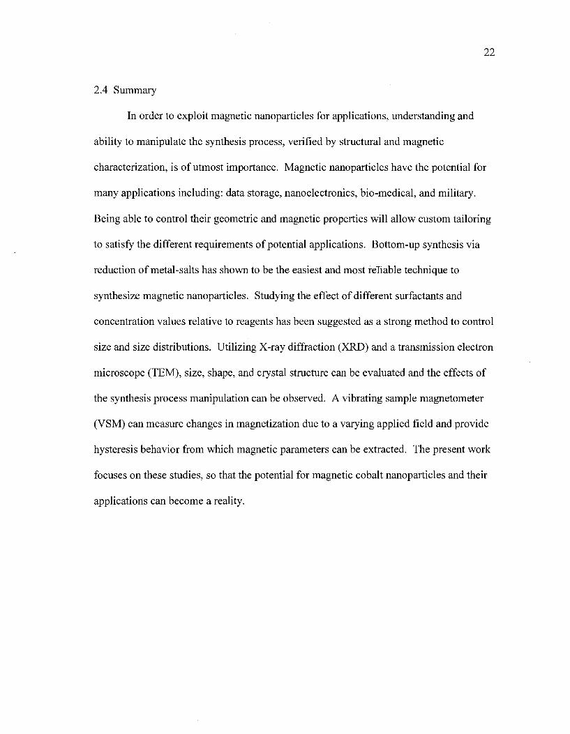
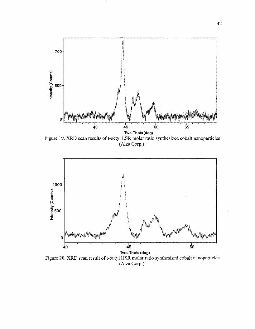
Figures 18-21 display the XRD scan results for cobalt nanoparticles synthesized

using trioctylphosphine (t-octyl) at a high surfactant-to-reagent (HSR) molar ratio, t-octyl

at low surfactant-to-reagent (LSR) molar ratio, tributylphosphine (t-butyl) at a HSR

molar ratio, and t-butyl at a LSR molar ratio, respectively.

45 Two-Theta (deg)

Figure 18. XRD scan result of t-octyl HSR molar ratio synthesized cobalt nanoparticles (Alza Corp.).

42

700

£ c 3 o O,

o c «

500H

o-

I I m

w W#^#*H^ ')'""'"'"i"'""""i"""""""r'"

40 ""r- '"""r >""*" r •"•x"""'""T"i"""""[""""

55 50 "">""" '""">" ' ""T

45 Two-Theta(deg)

Figure 19. XRD scan results of t-octyl LSR molar ratio synthesized cobalt nanoparticles (Alza Corp.).

45 Two-Theta (deg)

Figure 20. XRD scan result of t-butyl HSR molar ratio synthesized cobalt nanoparticles (Alza Corp.).

43

Two-Theta (cleg)

Figure 21. XRD scan result of t-butyl LSR molar ratio synthesized cobalt nanoparticles (SJSU).

All four scans show four peaks near the same relative angles. The t-butyl LSR

scan shows a peak at 26 = 41.727, at relatively low intensity. Table 5 summarizes the

major peaks and relative intensities seen in all four sample scans.

Table 5. XRD major peaks and relative intensities for cobalt nanoparticles synthesized using trioctylphosphine (t-octyl) at a high surfactant-to-reagent (HSR) molar ratio, t-octyl

at low surfactant-to-reagent (LSR) molar ratio, tributylphosphine (t-butyl) at a HSR molar ratio,

t-octyl HSR

29 44.5943 46.1929 47.1700 49.6428

Rel. Int. (%)

100.00 23.88 32.60 15.50

and t-buty t-octyl LSR

29 44.5195 45.6878 47.1106 49.5219

Rel. Int. (%)

100.00 16.42 29.44 16.23

at a LSR molar ratio. t-butyl HSR

29 44.6469 46.2646 47.1535 49.6164

Rel. Int. (%)

100.00 25.25 32.87 17.84

t-butyl LSR

29 41.727 44.504 46.217 47.013

.••'.••'• ,; ;•' :,:'.":' .;* .' s- ..'.• ?,:;" \t--.,' ..•• 49.495

Rel. Int. (%) 6.30

100.00 29.30 34.90 16.10

44

Re-arranging and using Bragg's Law in Equation 4, the observed d-spacing was

calculated for each of these peaks. Table 6 displays the d-spacings for the largest

diffraction peaks for all four sets of syntheses conditions.

d = -2sin#

Equation 4

Table 6. Observed d-spacings for cobalt nanoparticles at largest diffraction angle.

Condition t-octyl HSR t-octyl LSR t-butyl HSR t-butyl LSR

Peak (29) 49.6248 49.5219 49.6164 49.4950

d-spacing (A) 1.8350 1.8392 1.8359 1.8401

The results in Table 6 show d-spacing values very similar to each other, which is

as expected since the major peak angles are very similar.

Using Equation 5 with the assumption a cubic structure, the observed d-spacings,

and the lattice parameter of cobalt, each diffraction peak in Table 4 was indexed to a

crystal plane. Sun et al. have reported a lattice parameter of 6.30 A for the e-cobalt

structure [16]. Table 7 displays plane indexing results based on matching sin (0) to

(l2/4a2)(h2+k2+l2) in Equation 5.

1 _4s in 2 6>_/z 2 +£ 2 +/ 2

d2 ~ X2 ~~ a2 Equation 5

45

Table 7. Plane indexin t-octyl HSR

sin2(9) Match t-octyl LSR

sin2(0) Match

g results for cobalt nanoparticles. t-butyl HSR

sin2(0) Match

0.1440 0.1539 0.1601 0.1761

0.1440 0.1539 0.1602 0.1760

0.1435 0.1507 0.1597 0.1754

0.1435 0.1507 0.1597 0.1754

0.1443 0.1543 0.1600 0.1760

0.1442 0.1543 0.1602 0.1760

t-butyl LSR sin2(0) 0.1268 0.1434 0.1540 0.1591 0.1752

Match 0.1266 0.1437 0.1540 0.1592 0.1751

Indexed Plane 111 442 620 620 311

Table 7 shows that the peaks in Figure 18-21 are associated with the (442), (620),

(620), and (311) crystal planes. This simplifies to the primitive planes: (221), (310),

(310), and (311) which is associated with the s-cobalt crystal structure [13,16,30]. The

scan in Figure 21, shows a peak at 29 = 41.727 which is associated with the (111) plane.

For the e-cobalt crystal structure, the (221) plane is known to show the greatest

level of diffraction intensity [13,16]. Table 8 summarizes the major peaks, relative

intensities and indexed planes for all four scans.

Table 8. Major peaks, scan intensities, and indexed planes for cobalt nanoparticles. t-octyl HSR

29

Rel. Int. (%)

t-octyl LSR

20

Rel. Int. (%)

t-butyl HSR

29

Rel. Int. (%)

44.5943 46.1929 47.1700 49.6428

100.00 23.88 32.60 15.50

44.5195 45.6878 47.1106 49.5219

100.00 16.42 29.44 16.23

44.6469 46.2646 47.1535 49.6164

100.00 25.25 32.87 17.84

t-buty

29 41.7270 44.5040 46.2170 47.0130 49.4950

LSR Rel. Int. (%) 6.30

100.00 29.30 34.90 16.10

Planes

hkl 111 442 620 620 311

The results in Table 8 display an excellent match with 100% relative intensity on

the (442) plane for all samples. The (221) and (310) planes are not seen in the XRD

pattern due to extinction, s-cobalt is a form of the [3-manganese crystal structure which

follows a fee cubic structure, however, with atoms at unequal distances from each other

[5]. For calculation purposes a typical fee structure is assumed, hence atomic locations

46

are known to be (0,0,0), QA, lA, 0), (lA, 0, V2), (0, lA, lA). Using Equation 6, the structure

factor can be calculated which provides information on extinction of planes.

F = fc+ fco exp[2m(0.5h + 0.5k + 01)] + fCo exp[2m(0h + 0.5k + 0.5/)] + fCo exp[2;ri(0.5A + 0k + 0.5/)] E q u a t i o n 6

In Equation 6, when the integer within the exponent is odd or even, the exponent

has a value of-1 or +1, respectively. The value of the atomic scattering factor, fc0, is

determined using tabulated data [19]. Plotting tabulated values of fa> versus diffraction

angle, the relationship in Equation 7 is established for the atomic scattering factor of

cobalt, fc0.

- 1 . 3 5 ^

fCo=25.35e A Equation 7

Tables 9-12, display the calculated structure factor, F, indicating planes which

diffract for trioctylphosphine and tributylphosphine synthesized nanoparticles,

respectively.

Table 9. Structure factor, F, for t-octyl HSR cobalt nanoparticles. t-octyl HSR

29 44.5943 46.1929 47.1700 49.6248

sin (0) / 1 0.2463 0.2546 0.2597 0.2724

f(Co) 18.1798 17.9759 17.8530 17.5499

F(Co) 72.7190 71.9035 71.4119 70.1996

Int.(rel) 100.00% 23.88% 32.60% 15.50%

Plane (hkl) 442 620 620 311

Table 10. Structure factor, F, for t-octyl LSR cobalt nanoparticles. t-octyl LSR

20

44.5195

45.6878

47.1106

49.5219

sin (0) /

0.2459

0.2520 0.2594

0.2719

f(Co)

18.1894

18.0399

17.8604

17.5624

F(Co)

72.7575

72.1597

71.4416

70.2498

Int.(rel)

100.00%

16.42%

29.44%

16.23%

Plane

(hkl)

442

620

620

311

47

Table 11. Structure factor, F, for t-butyl HSR cobalt nanoparticles.

t-butyl HSR

29 sin (9) / X f(Co) F(Co) Int(rel)

44.6469

46.2646

47.1535

49.6164

0.2465

0.2550

0.2596

0.2723

18.1730

17.9668

17.8550

17.5509

72.6920

71.8673

71.4202

70.2037

100.00%

25.25%

32.87%

17.84%

Plane

(hkl)

111

442

620

620

311

Table 12. Structure factor, F, for t-butyl LSR cobalt nanoparticles. t-butyl LSR

29 41.7270 44.5040 46.2170 47.0130 49.4950

sin (9) / 1 0.2312 0.2458 0.2548 0.2589 0.2717

f(Co) 18.5542 18.1914 17.9728 17.8726 17.5657

F(Co) 74.2169 72.7655 71.8913 71.4906 70.2629

Int.(rel) 6.30%

100.00% 29.30% 34.90% 16.10%

Plane (hkl) 111 442 620 620 311

From Sun et al., the lattice parameter for the s-cobalt structure is reported as 6.30

A [16]. To confirm Equation 5 is utilized to calculate the observed lattice parameter for

the indexed planes for e-cobalt. Table 13 displays the observed lattice parameter for each

indexed plane for each synthesis condition. At the largest 29 value, the results show a

lattice parameter of 6.2983, 6.2995, 6.2993, and 6.2974 A for t-octyl HSR, t-octyl LSR, t-

butyl HSR, t-butyl LSR synthesis conditions, respectively. The calculated lattice

parameters at the largest diffraction peaks are within 0.05% of the value reported by Sun

etal.

48

Table 13. Observed lattice parameter for indexed planes s-cobalt nanoparticles.

Plane (hkl) 111

442 -221 620-310 620-310

311

t-octyl HSR (A) t-octyl LSR (A) t-butyl HSR

(A)

6.3003 6.2996 6.3013 6.2983

6.3008 6.3002 6.2995 6.2995

6.2992 6.2997 6.3033 6.2993

t-butyl LSR (A) 6.2946 6.3067 6.2997 6.3027 6.2974

The lattice parameters calculated in Table 13, however, do not account for

systematic error associated with the analysis. The systematic error results because the x-

ray focused beam is not in the plane of the sample; hence, the entirety of the sample is

not at the focal point of the beam. This systematic error is larger at low angles and

should be accounted for in order to have a more precise lattice parameter value [19].

Assuming that the largest source of error in the measurement is the displacement of the

sample from the diffractometer axis, an extrapolation of the lattice parameter can be

made from Equation 8. This corrective method only applies to Bragg-Brentano geometry

[19]. Hence, it is not utilized for t-butyl LSR which was scanned using parallel beam

alignment.

/ c o s 2 # T- *• o

a - a0 + a0k Equation 8

sin^

In Equation 8, a is the observed lattice parameter from indexed planes listed in

Table 13, 0 is the diffraction angle, and ao is the calculated lattice parameter. A plot of a

vs. (cos2 0)/(sin 0) for t-octyl HSR, t-octyl LSR, and t-butyl HSR molar ratio synthesis

conditions is displayed in Figure 22.

49

6.310

6.305

6.300

6.295

-•—t-octyl HSR ••- t-octyJLSR •it- t-bntvl HSR

6 290 i .900 2,000 2.100

(cos2 0)/{>in 0)

2.20 2.300

Figure 22. Corrected lattice parameter vs. diffraction angle for t-octyl HSR, t-octyl LSR, and t-butyl HSR molar ratio synthesized e-cobalt nanoparticles. R2=0.90, 0.92, 0.81,

respectively.

Linear fitted lines to the data in Figure 22 yield an extrapolation to the y-intercept

which is a corrected lattice parameter value. Table 14 summarizes the corrected lattice

parameter values for all synthesis conditions. The results in Table 14 indicate that the

corrected lattice parameters are within 0.25% of the value reported by Sun et al.

Table 14. Corrected lattice parameter for all cobalt nanoparticle syntheses conditions.

Condition t-octyl HSR t-octyl LSR t-butyl HSR t-butyl LSR

Corrected Lattice Parameter, a (A) 6.2860 6.2900 6.3030 N/A

50

The sample utilized in this analysis is assumed to be a randomly oriented powder.

In order to evaluate the nature of randomization, intensity is calculated using Equation 9

and compared to the results of the scan.

ha ~ \F\ pLPe~2M Equation 9

In Equation 9, F is the structure factor, p is the multiplicity factor, LP is the

Lorenz Polarization factor, and M is the temperature factor. The structure factor results

for all syntheses conditions are provided in Tables 9-12. The multiplicity factor is

acquired from reference tables and the temperature factor, M, is determined by Equation

10.

x, riisoor M =

A®

In Equation 10, T is temperature of the sample taken to be 298K, A is the atomic

weight, 58.933, 0 is the Debeye temperature which is 385K for cobalt, cp(x) is acquired

from reference tables [19], x is defined as T/ 0, 9 is the diffraction angle, and X is 1.5406

A.

Table 15 displays the calculated intensity results along with the results from the

scan. The calculated intensity results are normalized to the highest intensity plane

(422/221) to get relative intensity. The calculated results and scan results indicate that

the (442) is the strongest intensity plane. However, there is a significant difference in

relative intensities when comparing the calculated and observed intensities for the (620)

and (311) planes. The calculated intensity indicates a strong diffraction intensity is

expected, however, the observed relative intensities indicate a sharp drop-off from the

^(x) + | ' s i n # v

X Equation 10

51

(442) to the (620) and (311) planes. This result is consistent across all synthesis

conditions.

Table 15. Calculated vs. scan relative intensity results for cobalt nanoparticles.

Planes (hkl) 111 442 620 620 311

t-octyl HSR 1/1(442)

Calc. (%)

100.00 90.29 84.94 73.14

I/Io Obs. (%)

100.00 23.88 32.60 15.50

t-octy 1/1(442)

Calc. (%)

LSR I/Io Obs. (%)

t-butyl 1/1(442)

Calc. (%)

100.00 92.78 84.84 73.24

100.00 16.42 29.44 16.23

100.00 90.19 85.31 73.43

HSR I/Io Obs. (%)

100.00 25.25 32.87 17.84

t-buty] 1/1(442)

Calc. (%)

40.07 100.00 89.63 85.27 73.28

I LSR I/Io Obs. (%) 6.30

100.00 29.30 34.90 16.10

4.2 Particle Imaging, Size, and Size Distribution Analysis

After attempting many different techniques, the best TEM results were acquired by

using samples which were prepared by the spray-method. In this method, isolated

solutions of cobalt nanoparticles were placed in a nebulizer. The nebulizer was utilized

to create a fine mist which was sprayed onto a TEM grid. Figure 23 displays a TEM

image of t-octyl HSR synthesized cobalt nanoparticles at 400,000 times magnification.

Figure 23. TEM image of t-octyl HSR molar ratio synthesis cobalt nanoparticles at 400Kx magnification, Bar = lOnm.

52

Figure 24 displays a TEM image of t-octyl LSR synthesized cobalt nanoparticles

at 140,000 times magnification.

Figure 24. TEM image of t-octyl LSR molar ratio synthesis cobalt nanoparticles at

140Kx magnification, Bar = lOnm.

Figure 25 displays a TEM image of t-butyl HSR synthesized cobalt nanoparticles

at 400,000 times magnification.

53

Figure 25. TEM image of t-butyl HSR molar ratio synthesis cobalt nanoparticles at 400Kx magnification, Bar = 25nm.

Figure 26 displays a TEM image of t-butyl HSR synthesized cobalt nanoparticles

at 400,000 times magnification.

Figure 26. TEM image of t-butyl LSR molar ratio synthesis cobalt nanoparticles at 400Kx magnification, Bar = 50nm.

Images were captured in sufficient quantity to be able to size at a minimum 1000

particles for each synthesis condition. UTHSCSA Image Tool 3 imaging software,

developed at the University of Texas Health Science Center at San Antonio, was utilized

54

to perform particle sizing analysis. Figure 27 displays a boxplot of size versus surfactant

utilized for cobalt nanoparticle synthesis.

20

15

I 10"

"^ .'; .I5-

t-OData t-B Data

Figure 27. Boxplot of size versus surfactant used for cobalt nanoparticle synthesis.

Figure 27 displays utilizing trioctylphosphine versus tributylphosphine yields a

smaller average nanoparticle size. Figure 28 displays a histogram of cobalt nanoparticle

size versus surfactant utilized. In Figure 28, the solid line indicates trioctylphosphine and

the dashed line indicates tributylphosphine.

f

*

55

250-

200-

> u g 150-3 or V it

100-

50-

0-

/ / / /

"——i 1 ^ — \ —

1 s 1 1

/ \ / \ 1 \

I \ 1 \ 1 \ 1 \ 1 \ 1 1

\ \ \ \

v \

\

1 1 :—i

2.5 5.0 7.5 10.0 12.5 15.0 17.5

Variable t-0 Data t-B Data

Lognormal

Figure 28. Lognormal histogram of cobalt nanoparticle size versus surfactant.

The results in Figures 27 and 28 show that utilizing trioctylphosphine as a

surfactant yields an average cobalt nanoparticle size of 8.05 ± 1.59 nm, whereas

tributylphosphine yields 13.65 ± 1.61 nm. This data set is further divided into a boxplot

of size versus t-octyl HSR, t-octyl LSR, t-butyl HSR, and t-butyl LSR synthesis

conditions, displayed in Figure 29.

56

20-

15-

S

C

I 10" ^

1

t-o HSR

E5

1-0 LSR l-B HSR t-B LSR

Figure 29. Boxplot of cobalt nanoparticle size versus synthesis condition.

Figure 29 displays that using a higher molar ratio of surfactant-to-reagent yields a

smaller average nanoparticle size. Figure 30 displays a histogram of size versus t-octyl

HSR, t-octyl LSR, t-butyl HSR, and t-butyl LSR synthesis conditions.

57

250-

ZBO"

gr i5o^ • ' c

V •3 .

• o r w t 100-

50-

o-* f ,: 2.5

1

5.0

/ \ / \ I i

/ \ '' '

1 V > ' '•< ^

1 \ > \ < : -

^ ^̂ .. _ -̂ * — i i i i i

Variable

t-0 HSR t-0 LSR t-BHSR

t-BLSR

7.5 10.0 12.5 15.0 17.5 D a t a Lognormal

Figure 30. Lognormal histogram of cobalt nanoparticle size versus surfactant and

synthesis condition.

The resultant nanoparticle sizes in Figures 29 and 30 are summarized in Table 16.

Table 16. Nanoparticle size for t-octyl HSR, t-octyl LSR, t-butyl HSR, and t-butyl LSR molar ratio syntheses conditions. Condition

t-octyl HSR

t-octyl LSR

t-butyl HSR

t-butyl LSR

Size (ran)

6.87 ±0.89

9.22 ±1.24

12.47 ±0.88

14.84 ±1.26

Population

1009

1009

1009

1009

4.3 VSM Analysis

VSM analysis was conducted in the Solid State Physics Laboratory, SCI250, at

San Jose State University. Samples utilized for XRD analysis were used directly for VSM

analysis. The samples are approximately 3-5mg in weight deposited on a 5x5mm silicon

substrate. For magnetic measurements, a field range of-10,000 to +10,000 Oe was

58

applied. Figure 31 displays moment versus field overlay for cobalt nanoparticles at all

syntheses conditions.

1 i"'« I

Figure 31. Normalized magnetization versus applied field for t-octyl HSR (solid black), t-octyl LSR (dashed black), t-butyl HSR (solid gray), and t-octyl LSR (dashed gray)

synthesis conditions. For all synthesis conditions, cobalt nanoparticles display ferromagnetic behavior

at room temperature.

The coercive fields for each synthesis condition were found to be between 390-

500 Oe. Smaller particles synthesized using trioctylphosphine displayed a lower

coercivity compared to larger particles synthesized using tributylphosphine. Table 17

summarizes the coercivity for all synthesis conditions.

Table 17. Coercive fields for cobalt nanoparticles. Condition

t-octyl HSR

t-octyl LSR

t-butyl HSR

t-butyl LSR

Mean Particle Size (nm)

6.87 ±0.89

9.22 ±1.22

12.47 ±0.88

14.84 ±1.26

Coercivity (Oe)

393.4

397.6

397.3

493.6

59

CHAPTER FIVE: DISCUSSION

5.1 XRD Pattern Analysis

The XRD pattern analysis results in Table 6 show that the observed d-spacing is

very similar for all synthesis conditions in this experiment. Table 7 shows that the plane

indexing for each synthesis condition matches with the (442) plane displaying the

strongest diffraction intensity with the (620) and (311) planes following. The t-butyl

LSR condition does show diffraction at low intensity at the (111) plane. This yields two

conclusions: first, all synthesis conditions yield the same crystal structure and second, the

crystal structure is not the hexagonal close packed structure found at ambient conditions

or the face-centered cubic (fee) structure observed at temperatures above 722 K, in bulk

cobalt. The pattern results for all synthesized samples show the (442), (620), and (311)

displaying the strongest intensity. These planes are indicative of a meta-stable structure,

s-cobalt, which is a form of the (3-manganese crystal structure. The (111) plane seen in

the t-butyl LSR sample is an occurrence due to two possible reasons: low energy stacking

faults yielding diffraction at (111) and possible oxidation. Solution based synthesis is not

thermodynamically controlled and hence low energy stacking faults are a probable

phenomena seen in nanoparticles [16]. The other scenario is the possibility of oxidation:

cobalt oxide has a NaCl crystal structure which would diffract at (111) planes with 20

values very close to the observed scan value. Since the intensity of the peak is low

relative to the others either could be a viable scenario, however, the sample does continue

to show strongest diffraction intensity in the (442), (620), and (311) planes, which

follows the s-cobalt symmetry. This crystal structure is a complex form of the primitive

60

cubic cell with 20 atoms within at unequal separation distances [16]. The primitive

planes which are characteristic of the s-cobalt structure are (221), (310), and (311).

Atomic scattering factor calculations based on Equation 6, which are summarized in

Tables 9-12 show that the first two planes, (221) and (310) are not seen in the diffraction

pattern due to systematic extinction. The scan results for each synthesis condition also

show that there are two peaks, both index to the (620) plane. This splitting could be due

to CUKOI and CUKH2 radiation; however, this is largely seen at higher wavelengths. A

more probable cause is low energy stacking faults in the crystal. The hexagonal closed

packed (hep) structure of cobalt has a diffraction peak which lies approximately 29=46.5

degrees which is very close to the first peak indexed at (620) in all synthesis conditions.

The lattice parameter reported by Sun et al. is 6.30 A [16]. In this study, at

highest diffraction angle, the results show a lattice parameter of 6.2983, 6.2995, 6.2993,

and 6.2974 A for t-octyl HSR, t-octyl LSR, t-butyl HSR, t-butyl LSR synthesis

conditions, respectively. These values are within 0.05% of the reported value by Sun et

al. The observed lattice parameter does not take into account systematic error which can

be corrected for samples characterized using Bragg-Brentano geometry. The results from

this calculation yield a corrected lattice parameter of 6.286, 6.290, and 6.303, for t-octyl

HSR, t-octyl LSR, t-butyl HSR synthesis conditions, respectively. The scan of t-butyl

LSR was done using parallel beam geometry for which the corrected lattice parameter

analysis is invalid. The corrected lattice parameter values are within 0.25% of that

reported by Sun et al.

61

In Table 15, the calculated intensity results are shown versus the actual intensity

results from each synthesis condition scan. The results in Table 15 show that calculated

results and scan results indicate that the (442) is the strongest intensity plane across all

syntheses conditions. There is a significant difference in relative intensities when

comparing the calculated and observed intensities for the (620) and (311) planes. The

calculated intensity indicate a strong diffraction intensity is expected, however, the

observed relative intensities indicate a sharp drop-off from the (442) to the (620) and

(311) planes. This result is consistent across all synthesis conditions. This result is

indicative that the samples in all syntheses conditions are not randomized powders,

rather, they have a preference in orientation which is consistent across all conditions and

shows alignment to the strongest diffracting plane, (442).

5.2 TEM, Sizing and Size Distribution Analysis

In Figures 23-26 TEM scans for each synthesis condition display cobalt

nanoparticles in discrete hexagonal networks across the TEM grid sections. This

hexagonal network is formed on a consistent basis and the scans display particles within

the network are separated by an average range of 2-5 nm. The density of the network is

largely dictated by the amount of polar to non-polar solvent washes performed. The

number of washes yields a purified dilute solution. Figures 23, 25, and 26 are

characteristic of solutions washed 3-5 times. Figure 24 represents a solution which

underwent a series of 7 washes yielding a less dense string network. This is indicative

that 3-5 wash cycles yields a dense network of nanoparticles and further wash cycles

yield nanoparticle loss yielding less dense networks.

62

Sizing results in Figure 27 and 28 show a boxplot and histogram of t-octyl

synthesized versus t-butyl synthesized nanoparticles, respectively. The boxplot and

histogram show visual evidence of distinction between the t-butyl and t-octyl synthesized

particles. The histogram was plotted using a lognormal fit in order to exploit asymmetry;

however, the results in Figure 28 display a Gaussian distribution with mild deviations for

both groups of nanoparticles. Figures 29 and 30 display a further breakdown of the

overall data to the four synthesis conditions: t-octyl HSR, t-octyl LSR, t-butyl HSR, and

t-octyl LSR. The histogram in Figure 30 was also plotted using a lognormal fit to exploit

any form of asymmetry; however, again the distributions are Gaussian with mild

deviations. To compare the mean particle size among the groups, a two sample t-test

assuming unequal variances analysis was conducted. The analysis is based on a two-tail

distribution with a 99% confidence level. The results are summarized in Table 18.

Table 18. P(two-tail) two samples assuming unequal variances at 99% confidence matrix

t-octyl All

t-octyl HSR

t-octyl LSR

t-butyl HSR

t-butyl LSR

t-butyl All

tor comp t-octyl

All

<0.1%

<0.1%

<0.1%

aring the avt t-octyl HSR

<0.1%

<0.1%

<0.1%

<0.1%

;rage size ot t-octyl LSR

<0.1%

<0.1%

<0.1%

<0.1%

cobalt nano t-butyl HSR

<0.1%

<0.1%

<0.1%

<0.1%

particles. t-butyl LSR

<0.1%

<0.1%

<0.1%

<0.1%

t-butyl All

<0.1%

<0.1%

<0.1%

Table 18 displays comparisons between all t-test combinations. First combined

data for t-octyl is compared to t-butyl synthesis. The results indicate the probability that

63

the mean particle size is different between t-octyl versus t-butyl based synthesis due to

chance is less than 0.1%. Conversely, the probability that the two mean particles sizes

are different due to the surfactant utilized is greater than 99%. Similarly comparing t-

octyl HSR mean versus t-octyl LSR mean particle size shows that the probability that the

two means are different due to the difference in surfactant-to-reagent ratio is greater than

99%. The results in comparing t-butyl HSR and t-butyl LSR synthesis conditions yields

the same result. For completeness, the other combinations were analyzed as well and all

indicate significant statistical differences.

5.3 VSM Analysis

The overlayed M-H graphs in Figure 31 display open hysteresis loops for all

syntheses conditions, indicating ferromagnetic behavior at room temperature. The results

in Table 17 show coercivity values between 390-500 Oe indicating that the synthesized

cobalt nanoparticles behave as single domain magnets. The coercivity can be seen

increasing with nanoparticle size, with smaller t-octyl synthesized particles displaying

lower coercive field compared to larger t-butyl synthesized particles.

64

CHAPTER SIX: SUMMARY AND CONCLUSION

6.1 Summary

In this study, cobalt nanoparticles were synthesized via high temperature thermal

oxidation and reduction of cobalt (II) chloride utilizing two surfactants; tributylphosphine

and trioctylphosphine at 2:1 and 4:1 surfactant-to-reagent molar ratios. An x-ray

diffractometer, transmission electron microscope, and a vibrating sample magnetometer

were used to analyze the synthesis product for elemental identification and crystal

structure, particle size and morphology, and magnetic behavior, respectively.

The XRD results of this study indicate that all synthesis conditions yield cobalt as

the final product. Crystallographic analysis indicates that all syntheses conditions yield a

meta-stable structure known as s-cobalt. For t-octyl HSR, t-octyl LSR, and t-butyl HSR

syntheses conditions, the corrected lattice parameters for s-cobalt were 6.2860, 6.2900,

and 6.3030 A, respectively. The t-butyl LSR sample was scanned using parallel beam

geometry and had an observed lattice parameter of 6.2974 A. These lattice parameter

values were found to be within 0.25% of the reported value by Sun et al.

TEM results of this study display the formation of spherical cobalt nanoparticles

with a dense metallic core surrounded by an organic shell for all syntheses conditions. A

TEM sample preparation method was developed which utilizes a series of polar and non-

polar solvent washes to isolate the product and a nebulizer to apply the nanoparticles to a

TEM grid. The results show the formation of discrete hexagonal networks across TEM

grid samples with an average separation distance of 2-5 nm between nanoparticles.

65

Results also show that increasing the number of washes yields a less dense string-like

network of nanoparticles.

Particle size analysis was conducted utilizing ImageTool software developed by

the University of Texas Health Science Center at San Antonio. The results show that

trioctylphosphine based synthesis yields an average particle size of 8.05 ± 1.59 nm and

tributylphosphine based synthesis yields 13.65 ± 1.61 nm. Further partitioning the results

into the four synthesis condition found an average size of 6.87 ± 0.89, 9.22 ± 1.24, 12.47

± 0.88, 14.84 ± 1.26 nm for t-octyl HSR, t-octyl LSR, t-butyl HSR, and t-butyl LSR

condition, respectively. Statistical analysis was performed to compare the means of each

synthesis condition and the results indicate that each mean is statistically significant.

Magnetic analysis was done at ambient temperature utilizing a vibrating sample

magnetometer, applying a field ranging from -10,000 to 10,000 Oe. For all syntheses

conditions, the results display open hysteresis loops indicative of ferromagnetic behavior

at room temperature. Coercivity was calculated to be between 390-500 Oe for all

syntheses conditions, indicative that the cobalt nanoparticles behave as single domain

magnets with smaller trioctylphosphine synthesized nanoparticles displaying lower

coercivity relative to larger nanoparticles synthesized by tributylphosphine.

6.2 Conclusions

All the objectives of this research were successfully met. Magnetic cobalt

nanoparticles were successfully synthesized via thermal oxidation-reduction of cobalt (II)

chloride. X-ray diffraction characterization displayed the formation of an s-cobalt

66

structure for all syntheses conditions. Analysis found a lattice parameter within 0.25% of

the literature reported 6.30 A.

By utilizing two surfactants with differing size alkyl side chains, it was demonstrated that

mean nanoparticle size can be controlled, with the bulkier trioctylphosphine yielding

smaller average nanoparticles. It was further demonstrated that varying the surfactant-to-

reagent molar ratio also serves to control mean particle size, with higher surfactant-to-

reagent molar ratio yielding small particles. Magnetic analysis displayed open hysteresis

loops for all syntheses conditions, indicating room-temperature ferromagnetic behavior.

Further analysis found that coercivity ranged from 390 to 500 Oe, with small

nanoparticles displaying lower coercive field relative to larger particles.

6.3 Future Work

The development of cobalt nanoparticles remains in its early phases. Synthesis

techniques and characterization methods have been proven. There are many objectives to

follow up in research in order to make cobalt nanoparticles a viable industrial product.

Stability is one of the foremost concerns to address. Current research has not

shown any demonstration of long-term stability of synthesized nanoparticles. In order to

be viable for marketable products, these nanoparticles have to be proven to be stable for

extended periods of time. Particle size, distribution, morphology, and agglomeration are

key parameters to monitor in order to understand and attack concerns of stability.

Disposal methods are a follow-up concerns. Magnetic nanoparticles such as

cobalt are toxic and adequate and appropriate methods for neutralization and disposal are

necessary in order to make manufacturing environmentally feasible. For industrial

67

applications, hazardous waste containment and disaster handling methods are crucial

criteria.

Scale-up is the utmost of facets to address. Current research has demonstrated

synthesis and product yields on a bench-scale. Future research must analyze the effects

of scale and how particle size, size control, morphology behave with increases in

production scale. Current research displays bench-scale synthesis yield of less than 20%

with most experimental studies yielding on the order of 1-5%. In order to be viable for

manufacturing yield has to achieve a minimum of 80%.

The field of nanotechnology products is immense; however, without proper

development of these technologies, there will be no fruition.

68

REFERENCES

1. Nanotechnology, [Online]. Available at http://www.webopedia.eom/TERM/N/nanotechnology.html (accessed 16 February 2006).

2. Lux Research, Inc., The Nanotechnology Report 2004, [Online]. Available at http://www.physorg.com/news842.html (accessed 10 February 2006).

3. Y.K. Su, CM. Shen, T.Z. Yang, H.T. Yang, H.L. Li and H.J. Gao, "Synthesis and Characterization of Monodisperse Cobalt Nanocrystals and Nanocrystalline Superlattices, " Advanced Nanomaterials and Nanodevices IUMRS-ICEM, pp. 486-500 (June 2002).

4. V.F. Puntes, K.M. Krishnan and A.P. Alivisatos, "Colloidal Nanocrystal Shape and Size Control: The Case of Cobalt, " Science, Vol. 291, pp. 2115-2117 (March 2001).

5. C.B. Murray, S. Sun, W. Gaschler, H. Doyle, T.A. Betley and C.R. Kagan, "Colloidal Synthesis of Nanocrystals and Nanocrystal Superlattices, " IBM Journal of Research and Development, Vol. 45, No. 1, pp. 47-56 (January 2001).

6. B.E. Warren, X-Ray Diffraction, (Dover Publications, Inc., New York, 1990), pp. 7-12,27-35.

7. R.L. Comstock, Introduction to Magnetism and Magnetic Recording, (John Wiley & Sons, Inc., New York, 1999), pp. 52-56.

8. R. Kairoutdinov, Methods for the Synthesis of Nanoparticles and Nanomaterials, [Online], Available at http://www.uaf.edu/chem/467Sp05/lecture20.pdf, (accessed 27 February 2006).

9. B. Chaudret, "Chemical Synthesis of Magnetic Metal Nanoparticles, " Ecole Franco-Roumaine: Magnetisme des systemes nanoscopiques et structures hybrides,pp. 1-15,(2003).

10. E. Sowka, M. Leonowicz, B. Andrzejewski, A.D. Pomogailo, and G.I. Dzhardimalieva, Cobalt nanoparticles processed by thermal decomposition of metal containing monomer, [Online], Available at http://materialsscience.pwr.wroc.pl/ap/articles/ms 2005 022.pdf, (accessed 27 February 2006).

11. V.L. Khmov, Semiconductor and Metal Nanocrystals Synthesis and Electronic and Optical Properties, (Marcel Dekker, Inc., New York, 2004), pp 1-61, 387-417.

12. Y.W. Zhao, R.K. Zheng, X.X. Zhang, and J.Q. Xiao, "A Simple Method to Prepare Uniform Co Nanoparticles, " IEEE Transactions on Magnetics, Vol. 39, No. 5, pp. 2764-2766, (September 2003).

13. H.T. Yang, Y.K. Su, CM. Shen, T.Z. Yang, and H.J. Gao, "Synthesis and magnetic properties of s-cobalt nanoparticles, " Surface and Interface Analysis, 36, John Wiley and Sons, Ltd., pp. 155-160, (2004).

14. N.T.K. Thanh, V.F. Puntes, L.D. Tung, and D.G. Fernig, "Peptides as capping ligandsfor in situ synthesis of water soluble Co nanoparticles for bioapplications, " Journal of Physics: Conference Series No. 17, pp. 70-76, (2005).

15. M. Respaud, J.M. Broto, H. Rakoto, A.R. Fert, L. Thomas, B. Barbara, M. Verelst, E. Snoeck, P. Lecante, A. Mosset, J. Osuna, T. Ould Ely, C. Amiens, And B. Chaudret, "Surface effects on the magnetic properties ofultrafine cobalt particles, " The American Physical Society Physical Review B, Vol. 57, No. 5, pp. 2925-2935 (February 1998).

16. S. Sun and C.B. Murray, "Synthesis ofmonodisperse cobalt nanocrystals and their assembly into magnetic superlattices, " Journal of Applied Physics, Vol. 85, No. 8, pp. 4325-4330, (April 1999).

17.1. Lisiecki and M.P. Pileni, "Synthesis of Weil-Defined and Low Size Distribution Cobalt Nanocrystals: The Limited Influence of Reverse Micelles, " Langmuir, 19, pp. 9486-9489 (2003).

18. University of Wisconsin-Madison, Materials Research Science and Engineering Center for Nanostructured Interfaces, X-Ray Diffraction and Scanning Probe Microscopy, [Online], Available at http://mrsec.wisc.edu/Edetc/modules/xray/X-raystm.pdf, (accessed 1 March 2006).

19. B.D. Cullity, S.R. Stock, Elements of X-Ray Diffraction 3rd Edition, (Prentice Hall, 2001)

20. P.J. Schields, Bragg's Law and Diffraction: How waves reveal the atomic structure of crystals, [Online], Available at

70

21. J.R. Connolly, Introduction to X-ray Powder Diffraction, [Online], Available at: http://epswww.unm.edu/xrd/xrdclass/01 -XRD-Intro.pdf, (accessed 10 March 2006).

22. E.V. Shevchenko, D.V. Talapin, A.L. Rogach, A. Kornowski, M. Haase, and H. Weller, "Colloidal Synthesis and Self-Assembly ofCoPts Nanocrystals, " Journal of American Chemical Society, 124, pp. 11480-11485, (2002).

23. The Hebrew University of Jerusalem, TEM Basics, [Online], Available at http://www.nanoscience.huji.ac.il/unit/tem basics.htm, (accessed 22 March 2006).

24. G.L. Williams, J.K. Vohs, J.J. Brege and B.D. Fahlman, "Supercritical Fluid Facilitated Growth of Copper and Aluminum Oxide Nanoparticles, " Journal of Chemical Education, Vol. 82, No. 5, pp. 771-774 (May 2005).

25. A. Minor, National Center for Electron Microscopy, Lawrence Berkeley National Laboratory, (2006)

26. J. Hormes, H. Modrow, H. Bonnemann and C.S.S.R. Kumar, "The influence of various coatings on the electronic, magnetic, and geometric properties of cobalt nanoparticles," Journal of Applied Physics, 97, pp. 10R102-1-10R102-6, (2005)

27. D. Speliotis, ADE Technologies, Inc., Getting the Most From Your Vibrating Sample Magnetometer, [Online], Available at http://www.dms-magnetics.com/pdf/vsmmost.pdf, (accessed 4 March 2006).

28. Wikipedia The Free Encyclopedia, Hysteresis, [Online], Available at http://en.wikipedia.org/wiki/Hysteresis, (accessed 15 March 2006)

29. J. Hormes, H. Modrow, H. Bonnemann and C.S.S.R. Kumar, "The influence of various coatings on the electronic, magnetic, and geometric properties of cobalt nanoparticles," Journal of Applied Physics, 97, pp. 10R102-1-10R102-6, (2005)

30. Y. Bao, M. Beerman, A.B. Pakhomov, and K.M. Krishnan, "Controlled crystalline structure and surface stability of cobalt nanocrystals," Journal of Physical Chemistry B, 109, pp. 7220-7222, (2005)