
six sigma green belt handbook.pdf
364
Statistical Quality Control for the Six Sigma Green Belt
-
Upload
ashok-sharma -
Category
Documents
-
view
319 -
download
26
Transcript of six sigma green belt handbook.pdf

Statistical Quality Control for the Six Sigma Green Belt
H1277 CH00_FM.indd iH1277 CH00_FM.indd i 3/8/07 6:12:26 PM3/8/07 6:12:26 PM

Also available from ASQ Quality Press:
Applied Statistics for the Six Sigma Green BeltBhisham C. Gupta and H. Fred Walker
The Certified Six Sigma Green Belt HandbookRoderick A. Munro, Matthew J. Maio, Mohamed B. Nawaz, Govindarajan Ramu, and Daniel J. Zrymiak
Transactional Six Sigma for Green Belts: Maximizing Service and Manufacturing ProcessesSamuel E. Windsor
The Executive Guide to Understanding and Implementing Lean Six Sigma: The Financial ImpactRobert M. Meisel, Steven J. Babb, Steven F. Marsh, & James P. Schlichting
Applying the Science of Six Sigma to the Art of Sales and MarketingMichael J. Pestorius
Six Sigma Project Management: A Pocket GuideJeffrey N. Lowenthal
Six Sigma for the Next Millennium: A CSSBB GuidebookKim H. Pries
The Certified Quality Engineer Handbook, Second EditionRoger W. Berger, Donald W. Benbow, Ahmad K. Elshennawy, and H. Fred Walker, editors
The Certified Quality Technician HandbookDonald W. Benbow, Ahmad K. Elshennawy, and H. Fred Walker
The Certified Manager of Quality/Organizational Excellence Handbook: Third EditionRussell T. Westcott, editor
Business Performance through Lean Six Sigma: Linking the Knowledge Worker, the Twelve Pillars, and BaldrigeJames T. Schutta
To request a complimentary catalog of ASQ Quality Press publications, call 800-248-1946, or visit our Web site at http://qualitypress.asq.org.
H1277 CH00_FM.indd iiH1277 CH00_FM.indd ii 3/8/07 6:12:26 PM3/8/07 6:12:26 PM
Statistical Quality Control for the Six Sigma Green Belt
Bhisham C. GuptaH. Fred Walker
ASQ Quality PressMilwaukee, Wisconsin
H1277 CH00_FM.indd iiiH1277 CH00_FM.indd iii 3/8/07 6:12:27 PM3/8/07 6:12:27 PM
American Society for Quality, Quality Press, Milwaukee 53203© 2007 by American Society for QualityAll rights reserved. Published 2007Printed in the United States of America12 11 10 09 08 07 06 5 4 3 2 1
Library of Congress Cataloging-in-Publication Data
Gupta, Bhisham C., 1942– Statistical quality control for the Six sigma green belt / Bhisham C.Gupta and H. Fred Walker. p. cm. Includes index. ISBN 978-0-87389-686-3 (hard cover : alk. paper) 1. Six sigma (Quality control standard) 2. Quality control—Statistical methods. I. Walker, H. Fred, 1963– II. Title.
TS156.G8674 2007 658.5′62—dc22 2007000315
No part of this book may be reproduced in any form or by any means, electronic, mechanical, photocopying, recording, or otherwise, without the prior written permission of the publisher.
Publisher: William A. TonyAcquisitions Editor: Matt MeinholzProject Editor: Paul O’MaraProduction Administrator: Randall Benson
ASQ Mission: The American Society for Quality advances individual, organizational, and community excellence worldwide through learning, quality improvement, and knowledge exchange.
Attention Bookstores, Wholesalers, Schools, and Corporations: ASQ Quality Press books, videotapes, audiotapes, and software are available at quantity discounts with bulk purchases for business, educational, or instructional use. For information, please contact ASQ Quality Press at 800-248-1946, or write to ASQ Quality Press, P.O. Box 3005, Milwaukee, WI 53201-3005.
To place orders or to request a free copy of the ASQ Quality Press Publications Catalog, including ASQ membership information, call 800-248-1946. Visit our Web site at www.asq.org or http://qualitypress.asq.org.
Printed on acid-free paper
H1277 CH00_FM.indd ivH1277 CH00_FM.indd iv 3/8/07 6:12:27 PM3/8/07 6:12:27 PM

In loving memory of my parents, Roshan Lal and Sodhan Devi. —Bhisham
In loving memory of my father, Carl Ellsworth Walker. —Fred
H1277 CH00_FM.indd vH1277 CH00_FM.indd v 3/8/07 6:12:27 PM3/8/07 6:12:27 PM

H1277 CH00_FM.indd viH1277 CH00_FM.indd vi 3/8/07 6:12:27 PM3/8/07 6:12:27 PM
vii
Contents
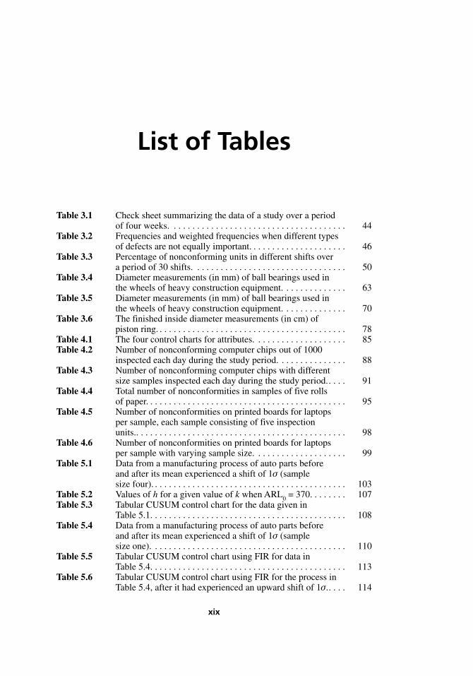
List of Figures . . . . . . . . . . . . . . . . . . . . . . . . . . . . . . . . . . . . . . . . . . . . . xiiiList of Tables . . . . . . . . . . . . . . . . . . . . . . . . . . . . . . . . . . . . . . . . . . . . . . xixPreface . . . . . . . . . . . . . . . . . . . . . . . . . . . . . . . . . . . . . . . . . . . . . . . . . . xxiAcknowledgments . . . . . . . . . . . . . . . . . . . . . . . . . . . . . . . . . . . . . . . . . . xxiii
Chapter 1 Introduction to Statistical Quality Control . . . . . . . . . . 11.1 Identifying the Tools of SQC . . . . . . . . . . . . . . . . . . . . . . . . . . . 21.2 Relating SQC to Applied Statistics and to DOE . . . . . . . . . . . . 21.3 Understanding the Role of Statistics in SQC . . . . . . . . . . . . . . 41.4 Making Decisions Based on Quantitative Data . . . . . . . . . . . . . 51.5 Practical versus Theoretical or Statistical Significance . . . . . . . 51.6 Why We Cannot Measure Everything . . . . . . . . . . . . . . . . . . . . 71.7 A Word on the Risks Associated with Making Bad
Decisions . . . . . . . . . . . . . . . . . . . . . . . . . . . . . . . . . . . . . . . . . . 7
Chapter 2 Elements of a Sample Survey . . . . . . . . . . . . . . . . . . . . . 112.1 Basic Concepts of Sampling . . . . . . . . . . . . . . . . . . . . . . . . . . . 11
Sampling Designs. . . . . . . . . . . . . . . . . . . . . . . . . . . . . . . . . . . 142.2 Simple Random Sampling . . . . . . . . . . . . . . . . . . . . . . . . . . . . . 15
2.2.1 Estimation of a Population Mean and Population Total 162.2.2 Confidence Interval for a Population Mean and
Population Total . . . . . . . . . . . . . . . . . . . . . . . . . . . . . . 202.2.3 Determination of Sample Size . . . . . . . . . . . . . . . . . . . 20
2.3 Stratified Random Sampling . . . . . . . . . . . . . . . . . . . . . . . . . . . 212.3.1 Estimation of a Population Mean and
Population Total . . . . . . . . . . . . . . . . . . . . . . . . . . . . . . 222.3.2 Confidence Interval for a Population Mean and
Population Total . . . . . . . . . . . . . . . . . . . . . . . . . . . . . . 242.3.3 Determination of Sample Size . . . . . . . . . . . . . . . . . . . 26
2.4 Systematic Random Sampling . . . . . . . . . . . . . . . . . . . . . . . . . . 272.4.1 Estimation of a Population Mean and
Population Total . . . . . . . . . . . . . . . . . . . . . . . . . . . . . . 28
H1277 CH00_FM.indd viiH1277 CH00_FM.indd vii 3/8/07 6:12:27 PM3/8/07 6:12:27 PM
viii Contents
2.4.2 Confidence Interval for a Population Mean and Population Total . . . . . . . . . . . . . . . . . . . . . . . . . . . 30
2.4.3 Determination of Sample Size . . . . . . . . . . . . . . . . . . . 302.5 Cluster Random Sampling . . . . . . . . . . . . . . . . . . . . . . . . . . . . . 32
2.5.1 Estimation of a Population Mean and Population Total . . . . . . . . . . . . . . . . . . . . . . . . . . . . . . 33
2.5.2 Confidence Interval for a Population Mean and Population Total . . . . . . . . . . . . . . . . . . . . . . . . . . . . . . 34
2.5.3 Determination of Sample Size . . . . . . . . . . . . . . . . . . . 37
Chapter 3 Phase I (Detecting Large Shifts)—SPC: Control Charts for Variables . . . . . . . . . . . . . . . . . . . . . . . . . . . . . 39
3.1 Basic Definition of Quality and Its Benefits . . . . . . . . . . . . . . . 403.2 SPC . . . . . . . . . . . . . . . . . . . . . . . . . . . . . . . . . . . . . . . . . . . . . . 41
Check Sheet . . . . . . . . . . . . . . . . . . . . . . . . . . . . . . . . . . . . . . . 43Pareto Chart . . . . . . . . . . . . . . . . . . . . . . . . . . . . . . . . . . . . . . . 45Cause-and-Effect (Fishbone or Ishikawa) Diagram . . . . . . . . . 47Defect Concentration Diagram. . . . . . . . . . . . . . . . . . . . . . . . . 48Run Chart . . . . . . . . . . . . . . . . . . . . . . . . . . . . . . . . . . . . . . . . . 50
3.3 Control Charts for Variables . . . . . . . . . . . . . . . . . . . . . . . . . . . 51Process Evaluation . . . . . . . . . . . . . . . . . . . . . . . . . . . . . . . . . . 51Action on Process . . . . . . . . . . . . . . . . . . . . . . . . . . . . . . . . . . . 51Action on Output . . . . . . . . . . . . . . . . . . . . . . . . . . . . . . . . . . . 51Variation . . . . . . . . . . . . . . . . . . . . . . . . . . . . . . . . . . . . . . . . . . 52Common Causes or Random Causes . . . . . . . . . . . . . . . . . . . . 52Special Causes or Assignable Causes. . . . . . . . . . . . . . . . . . . . 52Local Actions and Actions on the System . . . . . . . . . . . . . . . . 53Preparation for Use of Control Charts . . . . . . . . . . . . . . . . . . . 55Benefits of Control Charts . . . . . . . . . . . . . . . . . . . . . . . . . . . . 56Rational Samples for a Control Chart . . . . . . . . . . . . . . . . . . . 57ARL . . . . . . . . . . . . . . . . . . . . . . . . . . . . . . . . . . . . . . . . . . . . . 57OC Curve . . . . . . . . . . . . . . . . . . . . . . . . . . . . . . . . . . . . . . . . . 593.3.1 Shewhart X
– and R Control Charts . . . . . . . . . . . . . . . . . 60
3.3.2 Shewhart X– and R Control Charts When Process
Mean µ and Process Standard Deviation σ Are Known. . . . . . . . . . . . . . . . . . . . . . . . . . . . . . . . . . . . . . 68
3.3.3 Shewhart Control Chart for Individual Observations . . . . . . . . . . . . . . . . . . . . . . . . . . . . . . . . . 69
3.3.4 Shewhart X– and S Control Charts . . . . . . . . . . . . . . . . . 72
3.4 Process Capability . . . . . . . . . . . . . . . . . . . . . . . . . . . . . . . . . . . 79
Chapter 4 Phase I (Detecting Large Shifts)—SPC: Control Charts for Attributes . . . . . . . . . . . . . . . . . . . . . . . . . . . . 83
4.1 Control Charts for Attributes . . . . . . . . . . . . . . . . . . . . . . . . . . . 834.2 The p Chart: Control Chart for Fraction of Nonconforming
Units . . . . . . . . . . . . . . . . . . . . . . . . . . . . . . . . . . . . . . . . . . . . . 85Control Limits for the p Chart . . . . . . . . . . . . . . . . . . . . . . . . . 85
H1277 CH00_FM.indd viiiH1277 CH00_FM.indd viii 3/8/07 6:12:27 PM3/8/07 6:12:27 PM
Contents ix
4.2.1 The p Chart: Control Chart for Fraction Nonconforming with Variable Samples . . . . . . . . . . . . 89
4.3 The np Chart: Control Chart for Number of Nonconforming Units . . . . . . . . . . . . . . . . . . . . . . . . . . . . . . . . . . . . . . . . . . . . . 92
Control Limits for the np Control Chart. . . . . . . . . . . . . . . . . . 924.4 The c Chart (Nonconformities versus Nonconforming
Units) . . . . . . . . . . . . . . . . . . . . . . . . . . . . . . . . . . . . . . . . . . . . 934.5 The u Chart . . . . . . . . . . . . . . . . . . . . . . . . . . . . . . . . . . . . . . . . 96
Chapter 5 Phase II (Detecting Small Shifts)—SPC: Cumulative Sum, Moving Average, and Exponentially Weighted Moving Average Control Charts . . . . . . . . . . . . . . . . . . . . . . . . . . . . . . . . . 101
5.1 Basic Concepts of the CUSUM Control Chart . . . . . . . . . . . . . 102CUSUM Control Chart versus Shewhart X
–-R Control
Chart . . . . . . . . . . . . . . . . . . . . . . . . . . . . . . . . . . . . . . . . . . . . . 1025.2 Designing a CUSUM Control Chart . . . . . . . . . . . . . . . . . . . . . 104
5.2.1 Two- Sided CUSUM Control Chart Using Numerical Procedure . . . . . . . . . . . . . . . . . . . . . . . . . . . . . . . . . . . 106
5.2.2 The Fast Initial Response Feature for the CUSUM Control Chart . . . . . . . . . . . . . . . . . . . . . . . . . . . . . . . . 112
5.2.3 Combined Shewhart- CUSUM Control Chart . . . . . . . . 1155.2.4 CUSUM Control Chart for Controlling Process
Variability . . . . . . . . . . . . . . . . . . . . . . . . . . . . . . . . . . . 1165.3 The MA Control Chart . . . . . . . . . . . . . . . . . . . . . . . . . . . . . . . 1175.4 The EWMA Control Chart . . . . . . . . . . . . . . . . . . . . . . . . . . . . 120
Chapter 6 Process Capability Indices . . . . . . . . . . . . . . . . . . . . . . . 1276.1 Development of Process Capability Indices . . . . . . . . . . . . . . . 1276.2 PCI Cp . . . . . . . . . . . . . . . . . . . . . . . . . . . . . . . . . . . . . . . . . . . . 1306.3 PCI Cpk . . . . . . . . . . . . . . . . . . . . . . . . . . . . . . . . . . . . . . . . . . . . 1356.4 PCI Cpm . . . . . . . . . . . . . . . . . . . . . . . . . . . . . . . . . . . . . . . . . . . 1366.5 PCI Cpmk . . . . . . . . . . . . . . . . . . . . . . . . . . . . . . . . . . . . . . . . . . . 1386.6 PCI Cpnst . . . . . . . . . . . . . . . . . . . . . . . . . . . . . . . . . . . . . . . . . . . 139
Examples Comparing Cpnst with PCIs Cpk and Cpm. . . . . . . . . . 1416.6.1 Certain Features of the Capability Index Cpnst . . . . . . . 142
6.7 PCIs Pp and Ppk . . . . . . . . . . . . . . . . . . . . . . . . . . . . . . . . . . . . . 144
Chapter 7 Measurement Systems Analysis . . . . . . . . . . . . . . . . . . . 1477.1 Using SQC to Understand Variability . . . . . . . . . . . . . . . . . . . . 148
Variability in the Production or Service Delivery Process . . . . 148Variability in the Measurement Process . . . . . . . . . . . . . . . . . . 148
7.2 Evaluating Measurement System Performance . . . . . . . . . . . . . 1497.2.1 MSA Based on Range. . . . . . . . . . . . . . . . . . . . . . . . . . 1507.2.2 MSA Based on ANOVA . . . . . . . . . . . . . . . . . . . . . . . . 156
7.3 MCIs . . . . . . . . . . . . . . . . . . . . . . . . . . . . . . . . . . . . . . . . . . . . . 162MCI as a Percentage of Process Variation (MCIpv) . . . . . . . . . 162MCI as a Percentage of Process Specification (MCIps) . . . . . . 163
H1277 CH00_FM.indd ixH1277 CH00_FM.indd ix 3/8/07 6:12:27 PM3/8/07 6:12:27 PM
x Contents
Chapter 8 PRE-control . . . . . . . . . . . . . . . . . . . . . . . . . . . . . . . . . . . 1658.1 PRE- control Background. . . . . . . . . . . . . . . . . . . . . . . . . . . . . . 165
8.1.1 What Are We Trying to Accomplish with PRE- control?. . . . . . . . . . . . . . . . . . . . . . . . . . . . . . . . . 166
8.1.2 The Conditions Necessary for PRE- control to Be Valid. . . . . . . . . . . . . . . . . . . . . . . . . . . . . . . . . . . 166
8.2 Global Perspective on the Use of PRE- control (Understanding the Color- Coding Scheme) . . . . . . . . . . . . . . . 167
8.3 The Mechanics of PRE- control . . . . . . . . . . . . . . . . . . . . . . . . . 168Step 1: Ensure the Process Is Sufficiently Capable . . . . . . . . . 168Step 2: Establish the PRE- control Zones . . . . . . . . . . . . . . . . . 169Step 3: Verify That the Process Is Ready to Begin PRE- control . . . . . . . . . . . . . . . . . . . . . . . . . . . . . . . . . . . . . . . 169Step 4: Begin Sampling . . . . . . . . . . . . . . . . . . . . . . . . . . . . . . 169Step 5: Apply the PRE- control Rules . . . . . . . . . . . . . . . . . . . . 169
8.4 The Statistical Basis for PRE- control . . . . . . . . . . . . . . . . . . . . 1708.5 Advantages and Disadvantages of PRE- control . . . . . . . . . . . . 170
8.5.1 Advantages of PRE- control . . . . . . . . . . . . . . . . . . . . . 1718.5.2 Disadvantages of PRE- control . . . . . . . . . . . . . . . . . . . 171
8.6 What Comes After PRE- control? . . . . . . . . . . . . . . . . . . . . . . . 172
Chapter 9 Acceptance Sampling . . . . . . . . . . . . . . . . . . . . . . . . . . . . 1739.1 The Intent of Acceptance Sampling . . . . . . . . . . . . . . . . . . . . . 1739.2 Sampling Inspection versus 100 Percent Inspection . . . . . . . . . 1749.3 Sampling Concepts . . . . . . . . . . . . . . . . . . . . . . . . . . . . . . . . . . 175
9.3.1 Lot- by-Lot versus Average Quality Protection. . . . . . 1759.3.2 The OC Curve. . . . . . . . . . . . . . . . . . . . . . . . . . . . . . . 1759.3.3 Plotting the OC Curve . . . . . . . . . . . . . . . . . . . . . . . . 1769.3.4 Acceptance Sampling by Attributes . . . . . . . . . . . . . . 1779.3.5 Acceptable Quality Limit . . . . . . . . . . . . . . . . . . . . . . 1789.3.6 Lot Tolerance Percent Defective. . . . . . . . . . . . . . . . . 1789.3.7 Producer’s and Consumer’s Risks . . . . . . . . . . . . . . . 1789.3.8 Average Outgoing Quality . . . . . . . . . . . . . . . . . . . . . 1789.3.9 Average Outgoing Quality Limit . . . . . . . . . . . . . . . . 1799.3.10 Lot Size, Sample Size, and Acceptance Number . . . . 180
9.4 Types of Attribute Sampling Plans . . . . . . . . . . . . . . . . . . . . . . 1829.4.1 Single Sampling Plans . . . . . . . . . . . . . . . . . . . . . . . . . 1829.4.2 Double Sampling Plans. . . . . . . . . . . . . . . . . . . . . . . . . 1849.4.3 OC Curve for a Double Sampling Plan. . . . . . . . . . . . . 1849.4.4 Multiple Sampling Plans. . . . . . . . . . . . . . . . . . . . . . . . 1869.4.5 AOQ and AOQL for Double and Multiple Plans . . . . . 1869.4.6 Average Sample Number . . . . . . . . . . . . . . . . . . . . . . . 186
9.5 Sampling Standards and Plans. . . . . . . . . . . . . . . . . . . . . . . . . . 1889.5.1 ANSI/ASQ Z1.4-2003 . . . . . . . . . . . . . . . . . . . . . . . . . 1889.5.2 Levels of Inspection . . . . . . . . . . . . . . . . . . . . . . . . . . . 1899.5.3 Types of Sampling . . . . . . . . . . . . . . . . . . . . . . . . . . . . 1919.5.4 Dodge- Romig Tables . . . . . . . . . . . . . . . . . . . . . . . . . . 193
H1277 CH00_FM.indd xH1277 CH00_FM.indd x 3/8/07 6:12:27 PM3/8/07 6:12:27 PM
Contents xi
9.6 Variables Sampling Plans . . . . . . . . . . . . . . . . . . . . . . . . . . . . . 1939.6.1 ANSI/ASQ Z1.9-2003 . . . . . . . . . . . . . . . . . . . . . . . . . 194
9.7 Sequential Sampling Plans . . . . . . . . . . . . . . . . . . . . . . . . . . . . 1999.8 Continuous Sampling Plans . . . . . . . . . . . . . . . . . . . . . . . . . . . . 201
9.8.1 Types of Continuous Sampling Plans . . . . . . . . . . . . . . 2019.9 Variables Plan When the Standard Deviation Is Known . . . . . . 203
Chapter 10 Computer Resources to Support SQC: MINITAB . . . 22510.1 Using MINITAB—Version 14 . . . . . . . . . . . . . . . . . . . . . . . . 225
Getting Started with MINITAB . . . . . . . . . . . . . . . . . . . . . . 226Creating a New Worksheet . . . . . . . . . . . . . . . . . . . . . . . . . . 226Saving a Data File. . . . . . . . . . . . . . . . . . . . . . . . . . . . . . . . . 227Retrieving a Saved MINITAB Data File. . . . . . . . . . . . . . . . 227Saving a MINITAB Project. . . . . . . . . . . . . . . . . . . . . . . . . . 227Print Options . . . . . . . . . . . . . . . . . . . . . . . . . . . . . . . . . . . . . 228
10.2 The Shewhart Xbar- R Control Chart . . . . . . . . . . . . . . . . . . . 22810.3 The Shewhart Xbar- R Control Chart When Process
Mean µ and Process Standard Deviation σ Are Known . . . . . 23010.4 The Shewhart Control Chart for Individual Observations . . . 23010.5 The Shewhart Xbar- S Control Chart—Equal Sample
Size . . . . . . . . . . . . . . . . . . . . . . . . . . . . . . . . . . . . . . . . . . . . . 23110.6 The Shewhart Xbar- S Control Chart—Sample Size
Variable . . . . . . . . . . . . . . . . . . . . . . . . . . . . . . . . . . . . . . . . . 23310.7 Process Capability Analysis . . . . . . . . . . . . . . . . . . . . . . . . . . 23510.8 The p Chart: Control Chart for Fraction Nonconforming
Units . . . . . . . . . . . . . . . . . . . . . . . . . . . . . . . . . . . . . . . . . . . . 23810.9 The p Chart: Control Chart for Fraction Nonconforming
Units with Variable Sample Size . . . . . . . . . . . . . . . . . . . . . . 23910.10 The np Chart: Control Chart for Nonconforming Units . . . . 23910.11 The c Chart . . . . . . . . . . . . . . . . . . . . . . . . . . . . . . . . . . . . . . . 24010.12 The u Chart . . . . . . . . . . . . . . . . . . . . . . . . . . . . . . . . . . . . . . 24110.13 The u Chart: Variable Sample Size . . . . . . . . . . . . . . . . . . . . 24210.14 Designing a CUSUM Control Chart . . . . . . . . . . . . . . . . . . . 24310.15 The FIR Feature for a CUSUM Control Chart . . . . . . . . . . . 24510.16 The MA Control Chart . . . . . . . . . . . . . . . . . . . . . . . . . . . . . . 24510.17 The EWMA Control Chart . . . . . . . . . . . . . . . . . . . . . . . . . . 24710.18 Measurement System Capability Analysis . . . . . . . . . . . . . . 249
10.18.1 Measurement System Capability Analysis (Using Crossed Designs). . . . . . . . . . . . . . . . . . . . 250
Chapter 11 Computer Resources to Support SQC: JMP . . . . . . . 26111.1 Using JMP—Version 6.0 . . . . . . . . . . . . . . . . . . . . . . . . . . . . 261
Getting Started with JMP . . . . . . . . . . . . . . . . . . . . . . . . . . . 263Creating a New Data Table . . . . . . . . . . . . . . . . . . . . . . . . . . 264Opening an Existing JMP File . . . . . . . . . . . . . . . . . . . . . . . 265Saving JMP Files . . . . . . . . . . . . . . . . . . . . . . . . . . . . . . . . . 265Print Options . . . . . . . . . . . . . . . . . . . . . . . . . . . . . . . . . . . . . 266Using JMP Images for Reporting . . . . . . . . . . . . . . . . . . . . . 267
H1277 CH00_FM.indd xiH1277 CH00_FM.indd xi 3/8/07 6:12:27 PM3/8/07 6:12:27 PM
11.2 The Shewhart XBar and R Control Chart . . . . . . . . . . . . . . . 26811.3 The Shewhart XBar and S Control Chart—Equal
Sample Size . . . . . . . . . . . . . . . . . . . . . . . . . . . . . . . . . . . . . . 27011.4 The Shewhart XBar and S Control Chart—Sample Size
Variable . . . . . . . . . . . . . . . . . . . . . . . . . . . . . . . . . . . . . . . . . 27211.5 The Shewhart Control Chart for Individual
Observations . . . . . . . . . . . . . . . . . . . . . . . . . . . . . . . . . . . . . 27311.6 Process Capability Analysis . . . . . . . . . . . . . . . . . . . . . . . . . . 27511.7 The p Chart: Control Chart for Fraction Nonconforming
Units with Constant Sample Size . . . . . . . . . . . . . . . . . . . . . . 27711.8 The p Chart: Control Chart for Fraction Nonconforming
Units with Sample Size Varying . . . . . . . . . . . . . . . . . . . . . . 28111.9 The np Chart: Control Chart for Nonconforming Units . . . . 28111.10 The c Chart . . . . . . . . . . . . . . . . . . . . . . . . . . . . . . . . . . . . . . . 28211.11 The u Chart with Constant Sample Size . . . . . . . . . . . . . . . . 28411.12 The u Chart: Control Chart for Fraction Nonconforming
Units with Sample Size Varying . . . . . . . . . . . . . . . . . . . . . . 28611.13 The CUSUM Chart . . . . . . . . . . . . . . . . . . . . . . . . . . . . . . . . 28611.14 The Uniformly Weighted Moving Average Chart . . . . . . . . . 28811.15 The EWMA Control Chart . . . . . . . . . . . . . . . . . . . . . . . . . . 29011.16 Measurement System Capability Analysis . . . . . . . . . . . . . . 292
11.16.1 Measurement System Capability Analysis (Using Crossed Designs). . . . . . . . . . . . . . . . . . . . 293
Appendix Statistical Factors and Tables . . . . . . . . . . . . . . . . . . . . . 299
Bibliography . . . . . . . . . . . . . . . . . . . . . . . . . . . . . . . . . . . . . . . . . . . . . . 327Index . . . . . . . . . . . . . . . . . . . . . . . . . . . . . . . . . . . . . . . . . . . . . . . . . . . . 331
xii Contents
H1277 CH00_FM.indd xiiH1277 CH00_FM.indd xii 3/8/07 6:12:27 PM3/8/07 6:12:27 PM
xiii
List of Figures
Figure 1.1 The five tool types of SQC. . . . . . . . . . . . . . . . . . . . . . . . . . . . 2Figure 1.2 Relationship among applied statistics, SQC, and DOE. . . . . . 3Figure 1.3 Order of SQC topics in process or transactional Six Sigma. . . 4Figure 1.4 Detecting statistical differences. . . . . . . . . . . . . . . . . . . . . . . . 6Figure 1.5 Detecting practical and statistical differences. . . . . . . . . . . . . 6Figure 1.6 Sample versus population. . . . . . . . . . . . . . . . . . . . . . . . . . . . . 7Figure 3.1 Flowchart of a process. . . . . . . . . . . . . . . . . . . . . . . . . . . . . . . 41Figure 3.2 Pareto chart for data in Example 3.1.. . . . . . . . . . . . . . . . . . . . 45Figure 3.3 Pareto chart when weighted frequencies are used. . . . . . . . . . 47Figure 3.4 An initial form of a cause- and-effect diagram. . . . . . . . . . . . . 48Figure 3.5 A complete cause- and-effect diagram. . . . . . . . . . . . . . . . . . . 49Figure 3.6 A rectangular prism- shaped product that has been
damaged. . . . . . . . . . . . . . . . . . . . . . . . . . . . . . . . . . . . . . . . . . 49Figure 3.7 A run chart. . . . . . . . . . . . . . . . . . . . . . . . . . . . . . . . . . . . . . . . 50Figure 3.8 A control chart with a UCL and an LCL. . . . . . . . . . . . . . . . . 54Figure 3.9 OC curves for the x– chart with 3σ limits for different
sample sizes n. . . . . . . . . . . . . . . . . . . . . . . . . . . . . . . . . . . . . . 59Figure 3.10 The X– and R control charts, constructed using MINITAB,
for the ball bearing data in Table 3.4. . . . . . . . . . . . . . . . . . . . . . 65Figure 3.11 The MR control chart, constructed using MINITAB, for
the ball bearing data in Table 3.5. . . . . . . . . . . . . . . . . . . . . . . 71Figure 3.12 The X
– and S control charts, constructed using MINITAB,
for the ball bearing data in Table 3.4. . . . . . . . . . . . . . . . . . . . . 75Figure 3.13 The X
– and S control charts for variable sample sizes,
constructed using MINITAB, for the piston ring data in Table 3.6. . . . . . . . . . . . . . . . . . . . . . . . . . . . . . . . . . . . . . . . . . 77
Figure 3.14 Three illustrations of the concept of process capability, where (a) shows a process that is stable but not capable, (b) shows a process that is stable and barely capable, and (c) shows a process that is stable and capable. . . . . . . . . . . . . 80
Figure 4.1 MINITAB printout of the p chart for nonconforming computer chips, using trial control limits from the data in Table 4.2. . . . . . . . . . . . . . . . . . . . . . . . . . . . . . . . . . . . . . . . 89
Figure 4.2 MINITAB printout of the p chart for nonconforming chips with variable sample sizes, using trial control limits for the data in Table 4.3. . . . . . . . . . . . . . . . . . . . . . . . . . . . . . 91
H1277 CH00_FM.indd xiiiH1277 CH00_FM.indd xiii 3/8/07 6:12:28 PM3/8/07 6:12:28 PM
Figure 4.3 MINITAB printout of the np chart for nonconforming computer chips, using trial control limits for the data in Table 4.2. . . . . . . . . . . . . . . . . . . . . . . . . . . . . . . . . . . . . . . . 93
Figure 4.4 The c control chart of nonconformities for the data in Table 4.4. . . . . . . . . . . . . . . . . . . . . . . . . . . . . . . . . . . . . . . . 95
Figure 4.5 The u chart of nonconformities for the data in Table 4.5, constructed using MINITAB. . . . . . . . . . . . . . . . . . . . . . . . . . 99
Figure 4.6 The u chart of nonconformities for the data in Table 4.6, constructed using MINITAB. . . . . . . . . . . . . . . . . . . . . . . . . . 100
Figure 5.1 X–-R control chart for the data in Table 5.1. . . . . . . . . . . . . . . . 105Figure 5.2 CUSUM chart for the data in Table 5.1. . . . . . . . . . . . . . . . . . 105Figure 5.3 MINITAB printout of a two- sided CUSUM control chart
for the data in Table 5.1. . . . . . . . . . . . . . . . . . . . . . . . . . . . . . 109Figure 5.4 MINITAB printout of the X– control chart for individual
values in Table 5.4. . . . . . . . . . . . . . . . . . . . . . . . . . . . . . . . . . 111Figure 5.5 MINITAB printout of the CUSUM control chart for
individual values in Table 5.4. . . . . . . . . . . . . . . . . . . . . . . . . . 111Figure 5.6 MINITAB printout of the two- sided CUSUM control
chart for the data in Table 5.5 using FIR. . . . . . . . . . . . . . . . . 113Figure 5.7 MINITAB printout of the MA control chart for the data
in Table 5.4. . . . . . . . . . . . . . . . . . . . . . . . . . . . . . . . . . . . . . . . 120Figure 5.8 MINITAB printout of the EWMA control chart for the
data in Table 5.4. . . . . . . . . . . . . . . . . . . . . . . . . . . . . . . . . . . . 125Figure 6.1 Flowchart of a process. . . . . . . . . . . . . . . . . . . . . . . . . . . . . . . 128Figure 7.1 Approximate sampling distribution of sample statistics
X– with sample size five. . . . . . . . . . . . . . . . . . . . . . . . . . . . . . . 148
Figure 7.2 Components of total variation. . . . . . . . . . . . . . . . . . . . . . . . . . 149Figure 7.3 The distinction between accurate and precise, where (a) is
accurate and precise, (b) is accurate but not precise, (c) is not accurate but precise, and (d) is neither accurate nor precise. . . . . . . . . . . . . . . . . . . . . . . . . . . . . . . . . . . . . . . . . . . . . . . . 151
Figure 7.4 The linear relationship between the actual and the observed values. . . . . . . . . . . . . . . . . . . . . . . . . . . . . . . . . . . . . 152
Figure 7.5 Percent contribution of variance components for the data in Example 7.1. . . . . . . . . . . . . . . . . . . . . . . . . . . . . . . . . . . . . 159
Figure 7.6 X– and R charts for the data in Example 7.1. . . . . . . . . . . . . . . . 160
Figure 7.7 Interaction between operators and parts for the data in Example 7.1. . . . . . . . . . . . . . . . . . . . . . . . . . . . . . . . . . . . . . . 161
Figure 7.8 Scatter plot for measurements versus operators. . . . . . . . . . . . 161Figure 7.9 Scatter plot for measurements versus parts (bolts). . . . . . . . . . 162Figure 8.1 Relationships among the SQC tools. . . . . . . . . . . . . . . . . . . . . 165Figure 8.2 A barely capable process. . . . . . . . . . . . . . . . . . . . . . . . . . . . . 167Figure 8.3 PRE- control zones. . . . . . . . . . . . . . . . . . . . . . . . . . . . . . . . . . 168Figure 8.4 A process with process capability equal to one.. . . . . . . . . . . . 170Figure 9.1 An OC curve. . . . . . . . . . . . . . . . . . . . . . . . . . . . . . . . . . . . . . . 176Figure 9.2 AOQ curve for N = ∞, n = 50, c = 3. . . . . . . . . . . . . . . . . . . . . 180Figure 9.3 Effect on an OC curve of changing sample size (n) when
acceptance number (c) is held constant. . . . . . . . . . . . . . . . . . 181Figure 9.4 Effect of changing acceptance number (c) when sample
size (n) is held constant. . . . . . . . . . . . . . . . . . . . . . . . . . . . . . . 181Figure 9.5 Effect of changing lot size (N) when acceptance number
(c) and sample size (n) are held constant. . . . . . . . . . . . . . . . . 183
xiv List of Figures
H1277 CH00_FM.indd xivH1277 CH00_FM.indd xiv 3/8/07 6:12:28 PM3/8/07 6:12:28 PM
Figure 9.6 OC curves for sampling plans having the sample size equal to 10 percent of the lot size. . . . . . . . . . . . . . . . . . . . . . . . . . . . 183
Figure 9.7 OC curve for double sampling plan where n1 = 75, c1 = 0, r1 = 3, n2 = 75, c2 = 3, and r2 = 4. . . . . . . . . . . . . . . . . . . . . . . 185
Figure 9.8 AOQ curve for double sampling plan. . . . . . . . . . . . . . . . . . . . 186Figure 9.9 ASN curve for double sampling plan. . . . . . . . . . . . . . . . . . . . 188Figure 9.10 Switching rules for normal, tightened, and reduced
inspection. . . . . . . . . . . . . . . . . . . . . . . . . . . . . . . . . . . . . . . . . 190Figure 9.11 Structure and organization of ANSI/ASQ Z1.9-2003. . . . . . . . 195Figure 9.12 Decision areas for a sequential sampling plan. . . . . . . . . . . . . 199Figure 9.13 ANSI/ASQ Z1.4-2003 Table VIII: Limit numbers for
reduced inspection. . . . . . . . . . . . . . . . . . . . . . . . . . . . . . . . . . 205Figure 9.14 ANSI/ASQ Z1.4-2003 Table I: Sample size code letters. . . . . 206Figure 9.15 ANSI/ASQ Z1.4-2003 Table II- A: Single sampling plans
for normal inspection. . . . . . . . . . . . . . . . . . . . . . . . . . . . . . . . 207Figure 9.16 ANSI/ASQ Z1.4-2003 Table III- A: Double sampling
plans for normal inspection. . . . . . . . . . . . . . . . . . . . . . . . . . . 208Figure 9.17 ANSI/ASQ Z1.4-2003 Table IV- A: Multiple sampling
plans for normal inspection. . . . . . . . . . . . . . . . . . . . . . . . . . . 209Figure 9.18 4.20 ANSI/ASQ Z1.9-2003 Table A-2: Sample size
code letters. . . . . . . . . . . . . . . . . . . . . . . . . . . . . . . . . . . . . . . . 211Figure 9.19 ANSI/ASQ Z1.9-2003 Table C-1: Master table for normal
and tightened inspection for plans based on variability unknown (single specification limit—Form 1). . . . . . . . . . . . . 212
Figure 9.20 ANSI/ASQ Z1.9-2003 Table B-5: Table for estimating the lot percent nonconforming using standard deviation method. . . . . . . . . . . . . . . . . . . . . . . . . . . . . . . . . . . . . . . . . . . 213
Figure 9.21 ANSI/ASQ Z1.9-2003 Table B-3: Master table for normal and tightened inspection for plans based on variability unknown (double specification limit and Form 2—single specification limit). . . . . . . . . . . . . . . . . . . . . . . . . . . . . . . . . . 222
Figure 10.1 The welcome screen in MINITAB. . . . . . . . . . . . . . . . . . . . . . 226Figure 10.2 Showing the menu command options. . . . . . . . . . . . . . . . . . . . 227Figure 10.3 MINITAB window showing the Xbar-R Chart dialog
box. . . . . . . . . . . . . . . . . . . . . . . . . . . . . . . . . . . . . . . . . . . . . . 229Figure 10.4 MINITAB window showing the Xbar-R Chart - Options
dialog box. . . . . . . . . . . . . . . . . . . . . . . . . . . . . . . . . . . . . . . . . 230Figure 10.5 MINITAB window showing the Individuals- Moving
Range Chart dialog box. . . . . . . . . . . . . . . . . . . . . . . . . . . . . . . 231Figure 10.6 MINITAB window showing the Xbar-S Chart dialog
box. . . . . . . . . . . . . . . . . . . . . . . . . . . . . . . . . . . . . . . . . . . . . . 232Figure 10.7 MINITAB windows showing the Xbar- S Chart and
Xbar- S Chart - Options dialog boxes. . . . . . . . . . . . . . . . . . . 234Figure 10.8 MINITAB window showing the Capability Analysis
(Normal Distribution) dialog box. . . . . . . . . . . . . . . . . . . . . . . 237Figure 10.9 MINITAB windows showing the process capability
analysis. . . . . . . . . . . . . . . . . . . . . . . . . . . . . . . . . . . . . . . . . . . 237Figure 10.10 MINITAB window showing the P Chart dialog box. . . . . . . . 238Figure 10.11 MINITAB window showing the C Chart dialog box. . . . . . . . 241Figure 10.12 MINITAB window showing the U Chart dialog box. . . . . . . . 242Figure 10.13 MINITAB window showing the CUSUM Chart dialog
box. . . . . . . . . . . . . . . . . . . . . . . . . . . . . . . . . . . . . . . . . . . . . . 244
List of Figures xv
H1277 CH00_FM.indd xvH1277 CH00_FM.indd xv 3/8/07 6:12:28 PM3/8/07 6:12:28 PM
Figure 10.14 MINITAB window showing the CUSUM Chart - Options dialog box. . . . . . . . . . . . . . . . . . . . . . . . . . . . . . . . . . . . . . . . . 245
Figure 10.15 MINITAB window showing the Moving Average Chart dialog box. . . . . . . . . . . . . . . . . . . . . . . . . . . . . . . . . . . . . . . . . 246
Figure 10.16 MINITAB window showing the EWMA Chart dialog box. . . . . . . . . . . . . . . . . . . . . . . . . . . . . . . . . . . . . . . . . . . . . . 248
Figure 10.17 Screen showing the selections Stat > Quality Tools > Gage Study > Gage R&R Study (Crossed). . .. . . . . . . . . . . . . 252
Figure 10.18 Gage R&R Study (Crossed) dialog box. . . . . . . . . . . . . . . . . . 252Figure 10.19 Gage R&R Study (Crossed) - Options dialog box. . . . . . . . . . 253Figure 10.20 Percent contribution of variance components for the
data in Example 10.12. . . . . . . . . . . . . . . . . . . . . . . . . . . . . . . 257Figure 10.21 X– and R charts for the data in Example 10.12. . . . . . . . . . . . . . 258Figure 10.22 Interaction between operators and parts for the data in
Example 10.12. . . . . . . . . . . . . . . . . . . . . . . . . . . . . . . . . . . . . 258Figure 10.23 Scatter plot for measurements versus operators. . . . . . . . . . . . 259Figure 10.24 Scatter plot for measurements versus parts (bolts). . . . . . . . . . 259Figure 11.1 JMP Starter display. . . . . . . . . . . . . . . . . . . . . . . . . . . . . . . . . . 262Figure 11.2 JMP drop- down menus. . . . . . . . . . . . . . . . . . . . . . . . . . . . . . . 262Figure 11.3 JMP file processing commands. . . . . . . . . . . . . . . . . . . . . . . . 263Figure 11.4 JMP statistical analysis commands. . . . . . . . . . . . . . . . . . . . . . 264Figure 11.5 Creating a new data table. . . . . . . . . . . . . . . . . . . . . . . . . . . . . 264Figure 11.6 A new data table. . . . . . . . . . . . . . . . . . . . . . . . . . . . . . . . . . . . 265Figure 11.7 Opening an existing JMP file. . . . . . . . . . . . . . . . . . . . . . . . . . 266Figure 11.8 Saving a newly created JMP file. . . . . . . . . . . . . . . . . . . . . . . . 266Figure 11.9 Saving an existing JMP file. . . . . . . . . . . . . . . . . . . . . . . . . . . 267Figure 11.10 Printing JMP output. . . . . . . . . . . . . . . . . . . . . . . . . . . . . . . . . 267Figure 11.11 Generating an XBar and R chart. . . . . . . . . . . . . . . . . . . . . . . . 268Figure 11.12 XBar chart dialog box. . . . . . . . . . . . . . . . . . . . . . . . . . . . . . . . 269Figure 11.13 Generating an XBar and S chart. . . . . . . . . . . . . . . . . . . . . . . . 271Figure 11.14 XBar chart dialog box. . . . . . . . . . . . . . . . . . . . . . . . . . . . . . . . 271Figure 11.15 XBar and S chart dialog box. . . . . . . . . . . . . . . . . . . . . . . . . . . 273Figure 11.16 Generating a control chart for individual observations. . . . . . . 274Figure 11.17 IR chart dialog box. . . . . . . . . . . . . . . . . . . . . . . . . . . . . . . . . . 275Figure 11.18 Capability analysis based on an XBar and S chart
for Example 11.5. . . . . . . . . . . . . . . . . . . . . . . . . . . . . . . . . . . 277Figure 11.19 Process capability analysis dialog box. . . . . . . . . . . . . . . . . . . 278Figure 11.20 Process capability analysis output. . . . . . . . . . . . . . . . . . . . . . 279Figure 11.21 Generating a p chart. . . . . . . . . . . . . . . . . . . . . . . . . . . . . . . . . 280Figure 11.22 p chart dialog box. . . . . . . . . . . . . . . . . . . . . . . . . . . . . . . . . . . 280Figure 11.23 Generating a c chart. . . . . . . . . . . . . . . . . . . . . . . . . . . . . . . . . 282Figure 11.24 c chart dialog box. . . . . . . . . . . . . . . . . . . . . . . . . . . . . . . . . . . 283Figure 11.25 Generating a u chart. . . . . . . . . . . . . . . . . . . . . . . . . . . . . . . . . 284Figure 11.26 u chart dialog box. . . . . . . . . . . . . . . . . . . . . . . . . . . . . . . . . . . 285Figure 11.27 Generating a CUSUM chart. . . . . . . . . . . . . . . . . . . . . . . . . . . 287Figure 11.28 CUSUM chart dialog box. . . . . . . . . . . . . . . . . . . . . . . . . . . . . 287Figure 11.29 Specify Stats dialog box. . . . . . . . . . . . . . . . . . . . . . . . . . . . . . 288Figure 11.30 Generating a UWMA chart. . . . . . . . . . . . . . . . . . . . . . . . . . . . 289Figure 11.31 UWMA chart dialog box. . . . . . . . . . . . . . . . . . . . . . . . . . . . . 290Figure 11.32 Generating an EWMA chart. . . . . . . . . . . . . . . . . . . . . . . . . . . 291Figure 11.33 EWMA chart dialog box. . . . . . . . . . . . . . . . . . . . . . . . . . . . . . 292Figure 11.34 Initiating a Gage R&R. . . . . . . . . . . . . . . . . . . . . . . . . . . . . . . 295Figure 11.35 Gage R&R dialog box. . . . . . . . . . . . . . . . . . . . . . . . . . . . . . . 295
xvi List of Figures
H1277 CH00_FM.indd xviH1277 CH00_FM.indd xvi 3/8/07 6:12:28 PM3/8/07 6:12:28 PM

Figure 11.36 Completed Gage R&R dialog box. . . . . . . . . . . . . . . . . . . . . . 296Figure 11.37 Y, Response variability charts. . . . . . . . . . . . . . . . . . . . . . . . . . 296Figure 11.38 Continuing the Gage R&R. . . . . . . . . . . . . . . . . . . . . . . . . . . . 297Figure 11.39 Variance components. . . . . . . . . . . . . . . . . . . . . . . . . . . . . . . . 297Figure 11.40 Gage R&R dialog box. . . . . . . . . . . . . . . . . . . . . . . . . . . . . . . 297Figure 11.41 Gage R&R output. . . . . . . . . . . . . . . . . . . . . . . . . . . . . . . . . . . 298
List of Figures xvii
H1277 CH00_FM.indd xviiH1277 CH00_FM.indd xvii 3/8/07 6:12:28 PM3/8/07 6:12:28 PM

H1277 CH00_FM.indd xviiiH1277 CH00_FM.indd xviii 3/8/07 6:12:28 PM3/8/07 6:12:28 PM
xix
List of Tables
Table 3.1 Check sheet summarizing the data of a study over a period of four weeks. . . . . . . . . . . . . . . . . . . . . . . . . . . . . . . . . . . . . . 44
Table 3.2 Frequencies and weighted frequencies when different types of defects are not equally important. . . . . . . . . . . . . . . . . . . . . 46
Table 3.3 Percentage of nonconforming units in different shifts over a period of 30 shifts. . . . . . . . . . . . . . . . . . . . . . . . . . . . . . . . . 50
Table 3.4 Diameter measurements (in mm) of ball bearings used in the wheels of heavy construction equipment. . . . . . . . . . . . . . 63
Table 3.5 Diameter measurements (in mm) of ball bearings used in the wheels of heavy construction equipment. . . . . . . . . . . . . . 70
Table 3.6 The finished inside diameter measurements (in cm) of piston ring. . . . . . . . . . . . . . . . . . . . . . . . . . . . . . . . . . . . . . . . . 78
Table 4.1 The four control charts for attributes. . . . . . . . . . . . . . . . . . . . 85Table 4.2 Number of nonconforming computer chips out of 1000
inspected each day during the study period. . . . . . . . . . . . . . . 88Table 4.3 Number of nonconforming computer chips with different
size samples inspected each day during the study period. . . . . 91Table 4.4 Total number of nonconformities in samples of five rolls
of paper. . . . . . . . . . . . . . . . . . . . . . . . . . . . . . . . . . . . . . . . . . . 95Table 4.5 Number of nonconformities on printed boards for laptops
per sample, each sample consisting of five inspection units. . . . . . . . . . . . . . . . . . . . . . . . . . . . . . . . . . . . . . . . . . . . . . 98
Table 4.6 Number of nonconformities on printed boards for laptops per sample with varying sample size. . . . . . . . . . . . . . . . . . . . 99
Table 5.1 Data from a manufacturing process of auto parts before and after its mean experienced a shift of 1σ (sample size four). . . . . . . . . . . . . . . . . . . . . . . . . . . . . . . . . . . . . . . . . . 103
Table 5.2 Values of h for a given value of k when ARL0 = 370. . . . . . . . 107Table 5.3 Tabular CUSUM control chart for the data given in
Table 5.1. . . . . . . . . . . . . . . . . . . . . . . . . . . . . . . . . . . . . . . . . . 108Table 5.4 Data from a manufacturing process of auto parts before
and after its mean experienced a shift of 1σ (sample size one). . . . . . . . . . . . . . . . . . . . . . . . . . . . . . . . . . . . . . . . . . 110
Table 5.5 Tabular CUSUM control chart using FIR for data in Table 5.4. . . . . . . . . . . . . . . . . . . . . . . . . . . . . . . . . . . . . . . . . . 113
Table 5.6 Tabular CUSUM control chart using FIR for the process in Table 5.4, after it had experienced an upward shift of 1σ. . . . . 114
H1277 CH00_FM.indd xixH1277 CH00_FM.indd xix 3/8/07 6:12:28 PM3/8/07 6:12:28 PM
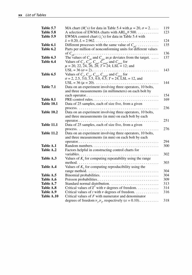
Table 5.7 MA chart (Mi’s) for data in Table 5.4 with µ = 20, σ = 2. . . . . 119Table 5.8 A selection of EWMA charts with ARL0
~= 500. . . . . . . . . . . . 123Table 5.9 EWMA control chart (zi’s) for data in Table 5.4 with
λ = 0.20, L = 2.962. . . . . . . . . . . . . . . . . . . . . . . . . . . . . . . . . . 124Table 6.1 Different processes with the same value of Cpk. . . . . . . . . . . . 135Table 6.2 Parts per million of nonconforming units for different values
of Cpk. . . . . . . . . . . . . . . . . . . . . . . . . . . . . . . . . . . . . . . . . . . . . 136Table 6.3 The values of Cpk and Cpm as µ deviates from the target. . . . . 137Table 6.4 Values of Cp, Cpk, Cpm, Cpmk, and Cpnst for
µ = 20, 22, 24, 26, 28; T = 24; LSL = 12; and USL = 36 (σ = 2).. . . . . . . . . . . . . . . . . . . . . . . . . . . . . . . . . . . 143
Table 6.5 Values of Cp, Cpk, Cpm, Cpmk, and Cpnst for σ = 2, 2.5, 3.0, 3.5, 4.0, 4.5; T = 24, LSL = 12, and USL = 36 (µ = 20). . . . . . . . . . . . . . . . . . . . . . . . . . . . . . . . . . 144
Table 7.1 Data on an experiment involving three operators, 10 bolts, and three measurements (in millimeters) on each bolt by each operator. . . . . . . . . . . . . . . . . . . . . . . . . . . . . . . . . . . . . . . 154
Table 8.1 PRE- control rules. . . . . . . . . . . . . . . . . . . . . . . . . . . . . . . . . . . 169Table 10.1 Data of 25 samples, each of size five, from a given
process. . . . . . . . . . . . . . . . . . . . . . . . . . . . . . . . . . . . . . . . . . . 236Table 10.2 Data on an experiment involving three operators, 10 bolts,
and three measurements (in mm) on each bolt by each operator. . . . . . . . . . . . . . . . . . . . . . . . . . . . . . . . . . . . . . . . . . . 251
Table 11.1 Data of 25 samples, each of size five, from a given process. . . . . . . . . . . . . . . . . . . . . . . . . . . . . . . . . . . . . . . . . . . 276
Table 11.2 Data on an experiment involving three operators, 10 bolts, and three measurements (in mm) on each bolt by each operator. . . . . . . . . . . . . . . . . . . . . . . . . . . . . . . . . . . . . . . . . . . 294
Table A.1 Random numbers. . . . . . . . . . . . . . . . . . . . . . . . . . . . . . . . . . . 300Table A.2 Factors helpful in constructing control charts for
variables . . . . . . . . . . . . . . . . . . . . . . . . . . . . . . . . . . . . . . . . . . 302Table A.3 Values of K1 for computing repeatability using the range
method. . . . . . . . . . . . . . . . . . . . . . . . . . . . . . . . . . . . . . . . . . . 303Table A.4 Values of K2 for computing reproducibility using the
range method. . . . . . . . . . . . . . . . . . . . . . . . . . . . . . . . . . . . . . 304Table A.5 Binomial probabilities. . . . . . . . . . . . . . . . . . . . . . . . . . . . . . . 304Table A.6 Poisson probabilities. . . . . . . . . . . . . . . . . . . . . . . . . . . . . . . . . 309Table A.7 Standard normal distribution. . . . . . . . . . . . . . . . . . . . . . . . . . 313Table A.8 Critical values of χ2 with ν degrees of freedom. . . . . . . . . . . . 314Table A.9 Critical values of t with ν degrees of freedom. . . . . . . . . . . . . 316Table A.10 Critical values of F with numerator and denominator
degrees of freedom ν1,ν2, respectively (α = 0.10). . . . . . . . . . . 318
xx List of Tables
H1277 CH00_FM.indd xxH1277 CH00_FM.indd xx 3/8/07 6:12:28 PM3/8/07 6:12:28 PM

xxi
Preface
Statistical Quality Control for the Six Sigma Green Belt was written as a desk reference and instructional aid for those individuals currently involved with, or preparing for involvement with, Six Sigma project
teams. As Six Sigma team members, Green Belts help select, collect data for, and assist with the interpretation of a variety of statistical or quantitative tools within the context of the Six Sigma methodology.
Composed of steps or phases titled Define, Measure, Analyze, Improve, and Control (DMAIC), the Six Sigma methodology calls for the use of many more statistical tools than is reasonable to address in one book. Accordingly, the intent of this book is to provide for Green Belts and Six Sigma team mem-bers a thorough discussion of the statistical quality control tools addressing both the underlying statistical concepts and the application. More advanced topics of a statistical or quantitative nature will be discussed in two additional books that, together with the first book in this series, Applied Statistics for the Six Sigma Green Belt, and this book, will comprise a four- book series.
While it is beyond the scope of this book and series to cover the DMAIC methodology specifically, this book and series focus on concepts, applica-tions, and interpretations of the statistical tools used during, and as part of, the DMAIC methodology. Of particular interest in the books in this series is an applied approach to the topics covered while providing a detailed discus-sion of the underlying concepts.
In fact, one very controversial aspect of Six Sigma training is that, in many cases, this training is targeted at the Six Sigma Black Belt and is all too commonly delivered to large groups of people with the assumption that all trainees have a fluent command of the statistically based tools and tech-niques. In practice this commonly leads to a good deal of concern and dis-comfort on behalf of trainees, as it quickly becomes difficult to keep up with and successfully complete Black Belt–level training without the benefit of truly understanding these tools and techniques.
So let us take a look together at Statistical Quality Control for the Six Sigma Green Belt. What you will learn is that these statistically based tools and techniques aren’t mysterious, they aren’t scary, and they aren’t overly difficult to understand. As in learning any topic, once you learn the basics, it is easy to build on that knowledge—trying to start without a knowledge of the basics, however, is generally the beginning of a difficult situation.
H1277 CH00_FM.indd xxiH1277 CH00_FM.indd xxi 3/8/07 6:12:29 PM3/8/07 6:12:29 PM

H1277 CH00_FM.indd xxiiH1277 CH00_FM.indd xxii 3/8/07 6:12:29 PM3/8/07 6:12:29 PM

xxiii
Acknowledgments
We would like to thank Professors John Brunette, Cheng Peng, Merle Guay, and Peggy Moore of the University of Southern Maine for reading the final draft line by line. Their comments and sugges-
tions have proven to be invaluable. We also thank Laurie McDermott, admin-istrative associate of the Department of Mathematics and Statistics of the University of Southern Maine, for help in typing the various drafts of the manuscript. In addition, we are grateful to the several anonymous reviewers, whose constructive suggestions greatly improved the presentations, and to our students, whose input was invaluable. We also want to thank Matt Mein-holz and Paul O’Mara of ASQ Quality Press for their patience and coopera-tion throughout the preparation of this project.
We acknowledge MINITAB for permitting us to reprint screen shots in this book. MINITAB and the MINITAB logo are registered trademarks of MINITAB. We also thank the SAS Institute for permitting us to reprint screen shots of JMP v. 6.0 (© 2006 SAS Institute). SAS, JMP, and all other SAS Institute product or service names are registered trademarks or trademarks of the SAS Institute in the United States and other countries. We would like to thank IBM for granting us permission to reproduce excerpts from Quality Institute manual entitled, Process Control, Capability and Improvement (© 1984 IBM Corporation and the IBM Quality Institute).
The authors would also like to thank their families. Bhisham is indebted to his wife, Swarn; his daughters, Anita and Anjali; his son, Shiva; his sons- in-law, Prajay and Mark; and his granddaughter, Priya, for their deep love and devotion. Fred would like to acknowledge the patience and support pro-vided by his wife, Julie, and sons, Carl and George, as he worked on this book. Without the encouragement of both their families, such projects would not be possible or meaningful.
—Bhisham C. Gupta —H. Fred Walker
H1277 CH00_FM.indd xxiiiH1277 CH00_FM.indd xxiii 3/8/07 6:12:29 PM3/8/07 6:12:29 PM

H1277 CH00_FM.indd xxivH1277 CH00_FM.indd xxiv 3/8/07 6:12:29 PM3/8/07 6:12:29 PM
1
Statistical quality control (SQC) refers to a set of interrelated tools used to monitor and improve process performance.
Definition 1.1 A process, for the purposes of this book, is a set of tasks or activities that change the form, fit, or function of one or more input(s) by adding value as is required or requested by a customer.
Defined in this manner, a process is associated with production and ser-vice delivery operations. Because Six Sigma applies to both production and service delivery/transactional operations, understanding and mastering the topics related to SQC is important to the Six Sigma Green Belt.
In this book, SQC tools are introduced and discussed from the perspec-tive of application rather than theoretical development. From this perspective, you can consider the SQC tools as statistical “alarm bells” that send signals when there are one or more problems with a particular process. As you learn more about the application of SQC tools, it will be helpful to understand that these tools have general guidelines and rules of thumb for both design and interpretation; however, these tools are intended to be tailored to each com-pany for use in a specific application. This means that when preparing to use SQC tools, choices must be made that impact how certain parameters within the tools are calculated, as well as how individual stakeholders involved with these tools actually interpret statistical data and results. Accordingly, choices related to the types of tools used, sample size and frequency, rules of interpre-tation, and acceptable levels of risk have a substantial impact on what comes out of these tools as far as usable information.
Critical to your understanding of SQC as a Six Sigma Green Belt is that SQC and statistical process control (SPC) are different. As noted earlier, SQC refers to a set of interrelated tools. SPC is but one of the tools that make up SQC. Many quality professionals continue to use the term SPC incorrectly by implying that SPC is used for process monitoring as a stand- alone tool. Prior to using SPC, we need to ensure that our process is set up correctly and, as much as possible, is in a state of statistical control. Likewise, once the process is in a state of statistical control, we need valid SPC data to facilitate
1
Introduction to Statistical Quality Control
H1277 ch01.indd 1H1277 ch01.indd 1 3/8/07 12:33:05 PM3/8/07 12:33:05 PM
2 Chapter One
our understanding of process capability and to enable the use of acceptance sampling.
1.1 Identifying the Tools of SQC
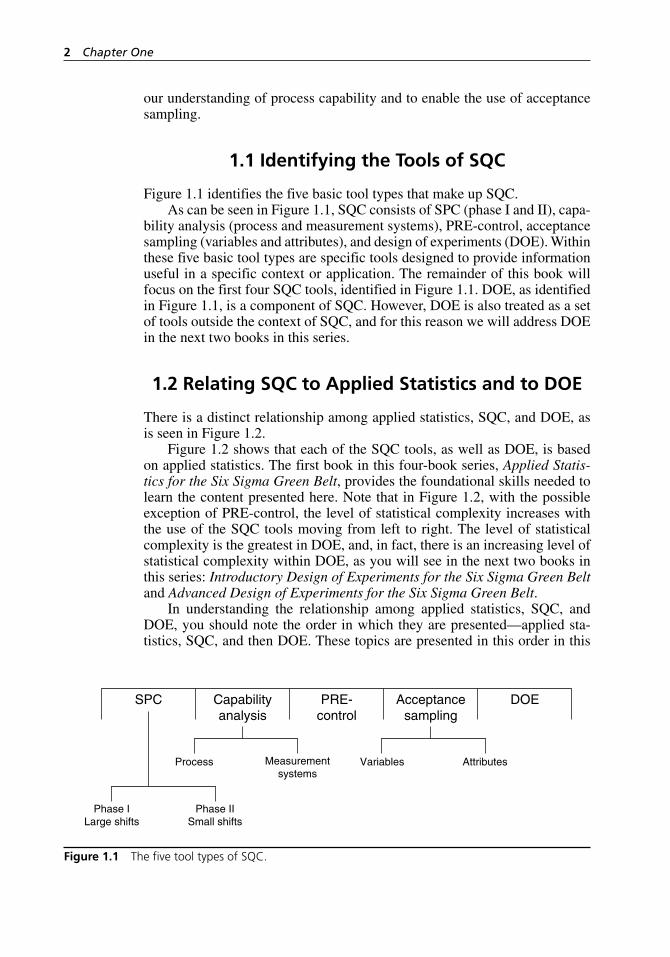
Figure 1.1 identifies the five basic tool types that make up SQC.As can be seen in Figure 1.1, SQC consists of SPC (phase I and II), capa-
bility analysis (process and measurement systems), PRE- control, acceptance sampling (variables and attributes), and design of experiments (DOE). Within these five basic tool types are specific tools designed to provide information useful in a specific context or application. The remainder of this book will focus on the first four SQC tools, identified in Figure 1.1. DOE, as identified in Figure 1.1, is a component of SQC. However, DOE is also treated as a set of tools outside the context of SQC, and for this reason we will address DOE in the next two books in this series.
1.2 Relating SQC to Applied Statistics and to DOE
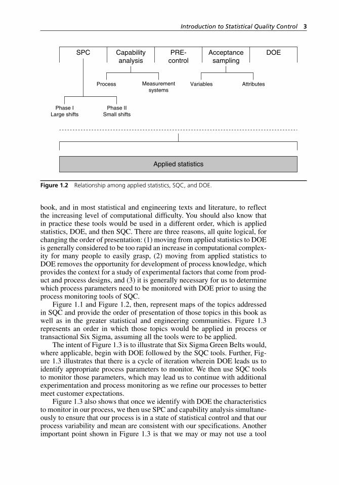
There is a distinct relationship among applied statistics, SQC, and DOE, as is seen in Figure 1.2.
Figure 1.2 shows that each of the SQC tools, as well as DOE, is based on applied statistics. The first book in this four- book series, Applied Statis-tics for the Six Sigma Green Belt, provides the foundational skills needed to learn the content presented here. Note that in Figure 1.2, with the possible exception of PRE- control, the level of statistical complexity increases with the use of the SQC tools moving from left to right. The level of statistical complexity is the greatest in DOE, and, in fact, there is an increasing level of statistical complexity within DOE, as you will see in the next two books in this series: Introductory Design of Experiments for the Six Sigma Green Belt and Advanced Design of Experiments for the Six Sigma Green Belt.
In understanding the relationship among applied statistics, SQC, and DOE, you should note the order in which they are presented—applied sta-tistics, SQC, and then DOE. These topics are presented in this order in this
SPC Capabilityanalysis
PRE-control
Acceptancesampling
DOE
Phase ILarge shifts
Phase IISmall shifts
Process Measurementsystems
Variables Attributes
Figure 1.1 The five tool types of SQC.
H1277 ch01.indd 2H1277 ch01.indd 2 3/8/07 12:33:05 PM3/8/07 12:33:05 PM
Introduction to Statistical Quality Control 3
book, and in most statistical and engineering texts and literature, to reflect the increasing level of computational difficulty. You should also know that in practice these tools would be used in a different order, which is applied statistics, DOE, and then SQC. There are three reasons, all quite logical, for changing the order of presentation: (1) moving from applied statistics to DOE is generally considered to be too rapid an increase in computational complex-ity for many people to easily grasp, (2) moving from applied statistics to DOE removes the opportunity for development of process knowledge, which provides the context for a study of experimental factors that come from prod-uct and process designs, and (3) it is generally necessary for us to determine which process parameters need to be monitored with DOE prior to using the process monitoring tools of SQC.
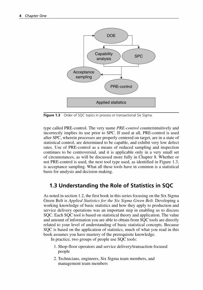
Figure 1.1 and Figure 1.2, then, represent maps of the topics addressed in SQC and provide the order of presentation of those topics in this book as well as in the greater statistical and engineering communities. Figure 1.3 represents an order in which those topics would be applied in process or transactional Six Sigma, assuming all the tools were to be applied.
The intent of Figure 1.3 is to illustrate that Six Sigma Green Belts would, where applicable, begin with DOE followed by the SQC tools. Further, Fig-ure 1.3 illustrates that there is a cycle of iteration wherein DOE leads us to identify appropriate process parameters to monitor. We then use SQC tools to monitor those parameters, which may lead us to continue with additional experimentation and process monitoring as we refine our processes to better meet customer expectations.
Figure 1.3 also shows that once we identify with DOE the characteristics to monitor in our process, we then use SPC and capability analysis simultane-ously to ensure that our process is in a state of statistical control and that our process variability and mean are consistent with our specifications. Another important point shown in Figure 1.3 is that we may or may not use a tool
SPC Capabilityanalysis
PRE-control
Acceptancesampling
DOE
Phase ILarge shifts
Phase IISmall shifts
Process Measurementsystems
Variables Attributes
Applied statistics
Figure 1.2 Relationship among applied statistics, SQC, and DOE.
H1277 ch01.indd 3H1277 ch01.indd 3 3/8/07 12:33:06 PM3/8/07 12:33:06 PM
4 Chapter One
type called PRE- control. The very name PRE-control counterintuitively and incorrectly implies its use prior to SPC. If used at all, PRE- control is used after SPC, wherein processes are properly centered on target, are in a state of statistical control, are determined to be capable, and exhibit very low defect rates. Use of PRE- control as a means of reduced sampling and inspection continues to be controversial, and it is applicable only in a very small set of circumstances, as will be discussed more fully in Chapter 8. Whether or not PRE- control is used, the next tool type used, as identified in Figure 1.3, is acceptance sampling. What all these tools have in common is a statistical basis for analysis and decision making.
1.3 Understanding the Role of Statistics in SQC
As noted in section 1.2, the first book in this series focusing on the Six Sigma Green Belt is Applied Statistics for the Six Sigma Green Belt. Developing a working knowledge of basic statistics and how they apply to production and service delivery operations was an important step in enabling us to discuss SQC. Each SQC tool is based on statistical theory and application. The value and amount of information you are able to obtain from SQC tools are directly related to your level of understanding of basic statistical concepts. Because SQC is based on the application of statistics, much of what you read in this book assumes you have mastery of the prerequisite knowledge.
In practice, two groups of people use SQC tools:
1. Shop-floor operators and service delivery/transaction-focused people
2. Technicians, engineers, Six Sigma team members, and management team members
SPCCapabilityanalysis
PRE-control
Acceptancesampling
DOE
Applied statistics
Figure 1.3 Order of SQC topics in process or transactional Six Sigma.
H1277 ch01.indd 4H1277 ch01.indd 4 3/8/07 12:33:06 PM3/8/07 12:33:06 PM
Introduction to Statistical Quality Control 5
Each group using SQC tools has different roles and responsibilities rela-tive to the use and implementation of the tools. For example, people in group 1 are commonly expected to collect data for, generate, and react to SQC tools. People in group 2 are commonly expected to design and implement SQC tools. They are also expected to critically analyze data from these tools and make decisions based on information gained from them.
1.4 Making Decisions Based on Quantitative Data
In practice, we are asked to make decisions based on quantitative and qualita-tive data on a regular basis.
Definition 1.2 Quantitative data are numerical data obtained from direct measurement or tally/count. Direct measurement uses a scale for measurement and reference, and tally/count uses direct observa-tion as a basis for summarizing occurrences of some phenomenon.
Definition 1.3 Qualitative data are nonnumerical data obtained from direct observation, survey, personal experience, beliefs, percep-tions, and perhaps historical records.
It is important to acknowledge that application of both quantitative and qualitative data has value and can be entirely appropriate in a professional work environment depending on the types of decisions we need to make. It is also important to acknowledge the difficulty in defending the use of qualitative data to make decisions in the design and process improvement efforts most commonly encountered by the Six Sigma Green Belt. Key, then, to obtaining the maximum value of information from SQC tools is realizing the power of quantitative data, because what can be directly measured can be validated and verified.
1.5 Practical versus Theoretical or Statistical Significance
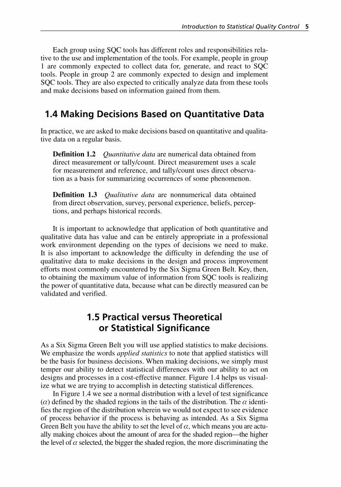
As a Six Sigma Green Belt you will use applied statistics to make decisions. We emphasize the words applied statistics to note that applied statistics will be the basis for business decisions. When making decisions, we simply must temper our ability to detect statistical differences with our ability to act on designs and processes in a cost- effective manner. Figure 1.4 helps us visual-ize what we are trying to accomplish in detecting statistical differences.
In Figure 1.4 we see a normal distribution with a level of test significance (α) defined by the shaded regions in the tails of the distribution. The α identi-fies the region of the distribution wherein we would not expect to see evidence of process behavior if the process is behaving as intended. As a Six Sigma Green Belt you have the ability to set the level of α, which means you are actu-ally making choices about the amount of area for the shaded region—the higher the level of α selected, the bigger the shaded region, the more discriminating the
H1277 ch01.indd 5H1277 ch01.indd 5 3/8/07 12:33:06 PM3/8/07 12:33:06 PM
6 Chapter One
test, and the more expensive it will be to make process improvement changes. While making any decisions related to α has financial implications, to under-stand practical differences we need to look at Figure 1.5.
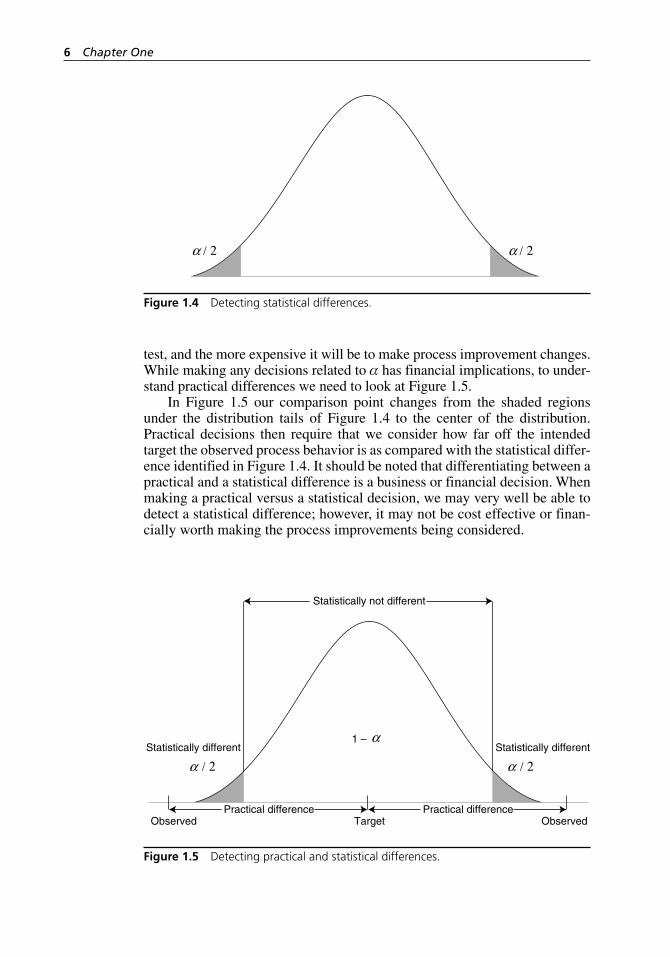
In Figure 1.5 our comparison point changes from the shaded regions under the distribution tails of Figure 1.4 to the center of the distribution. Practical decisions then require that we consider how far off the intended target the observed process behavior is as compared with the statistical differ-ence identified in Figure 1.4. It should be noted that differentiating between a practical and a statistical difference is a business or financial decision. When making a practical versus a statistical decision, we may very well be able to detect a statistical difference; however, it may not be cost effective or finan-cially worth making the process improvements being considered.
Figure 1.4 Detecting statistical differences.
Statistically not different
Statistically different Statistically different
Observed ObservedTargetPractical difference Practical difference
1 –
Figure 1.5 Detecting practical and statistical differences.
H1277 ch01.indd 6H1277 ch01.indd 6 3/8/07 12:33:06 PM3/8/07 12:33:06 PM
Introduction to Statistical Quality Control 7
1.6 Why We Cannot Measure Everything
Whether in process- oriented industries such as manufacturing or in transactional- oriented industries, the volume of operations is sufficiently large to prohibit measurement of all the important characteristics in all units of production or all transactions. And even if we could measure some selected quality characteristic in all units of production or in all transactions, it is well known that we simply would not identify every discrepancy or mistake. So managing a balance between the volume of measurement and the probability of making errors during the measurement process requires us to rely on the power of statistics.
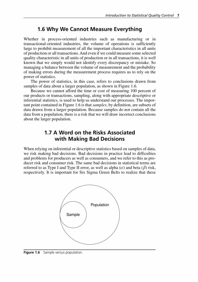
The power of statistics, in this case, refers to conclusions drawn from samples of data about a larger population, as shown in Figure 1.6.
Because we cannot afford the time or cost of measuring 100 percent of our products or transactions, sampling, along with appropriate descriptive or inferential statistics, is used to help us understand our processes. The impor-tant point contained in Figure 1.6 is that samples, by definition, are subsets of data drawn from a larger population. Because samples do not contain all the data from a population, there is a risk that we will draw incorrect conclusions about the larger population.
1.7 A Word on the Risks Associated with Making Bad Decisions
When relying on inferential or descriptive statistics based on samples of data, we risk making bad decisions. Bad decisions in practice lead to difficulties and problems for producers as well as consumers, and we refer to this as pro-ducer risk and consumer risk. The same bad decisions in statistical terms are referred to as Type I and Type II error, as well as alpha (α) and beta (β) risk, respectively. It is important for Six Sigma Green Belts to realize that these
Population
Sample
Figure 1.6 Sample versus population.
H1277 ch01.indd 7H1277 ch01.indd 7 3/8/07 12:33:06 PM3/8/07 12:33:06 PM
8 Chapter One
risks exist and that people from different functional areas within an organi-zation may use different terms to describe the same thing. Lastly, we must realize that choices made during the design of SQC tools, choices related to selection of consumer and producer risk levels, quite dramatically impact performance of the tools and the subsequent information they produce for decision making.
It is not enough to simply identify the risks associated with making bad decisions; the Six Sigma Green Belt must also know the following key points:
Sooner or later, a bad decision will be made
The risks associated with making bad decisions are quantified in probabilistic terms
α and β risks added together do not equal one
Even though α and β go in opposite directions (that is, if α increases, β decreases), there is no direct relationship between α and β
The values of α and β can be kept as low as we want by increasing the sample size
Definition 1.4 Probability is the chance that an event or outcome will or will not occur. Probability is quantified as a number between zero and one where the chance that an event or outcome will not occur in perfect certainty is zero and the chance that it will occur with perfect certainty is one. The chance that an event or outcome will not occur added to the chance that it will occur add up to one.
Definition 1.5 Producer risk is the risk of failing to pass a prod-uct or service delivery transaction on to a customer when, in fact, the product or service delivery transaction meets the customer qual-ity expectations. The probability of making a producer risk error is quantified in terms of α.
Definition 1.6 Consumer risk is the risk of passing a product or service delivery transaction on to a customer under the assump-tion that the product or service delivery transaction meets customer quality expectations when, in fact, the product or service delivery is defective or unsatisfactory. The probability of making a consumer risk error is quantified in terms of β.
A critically important point, and a point that many people struggle to under-stand, is the difference between the probability that an event will or will not occur and the probabilities associated with consumer and producer risk—they simply are not the same thing. As noted earlier, probability is the percent chance that an event will or will not occur, wherein the percent chances of an event occurring or not occurring add up to one. The probability associated with making an error for the consumer, quantified as β, is a value ranging
•
•
•
•
•
H1277 ch01.indd 8H1277 ch01.indd 8 3/8/07 12:33:07 PM3/8/07 12:33:07 PM

Introduction to Statistical Quality Control 9
between zero and one. The probability associated with making an error for the producer, quantified as α, is also a value between zero and one. The key here is that α and β do not add up to one. In practice, one sets an acceptable level of α and then applies some form of test procedure (some application of an SQC tool in this case) so that the probability of committing a β error is accept-ably small. So defining a level of α does not automatically set the level of β.
In closing, the chapters that follow discuss the collection of data and the design, application, and interpretation of each of the various SQC tools. You should have the following two goals while learning about SQC: (1) to master these tools at a conceptual level, and (2) to keep in perspective that the use of these tools requires tailoring them to your specific application while balanc-ing practical and statistical differences.
H1277 ch01.indd 9H1277 ch01.indd 9 3/8/07 12:33:07 PM3/8/07 12:33:07 PM

H1277 ch01.indd 10H1277 ch01.indd 10 3/8/07 12:33:07 PM3/8/07 12:33:07 PM
11
The science of sampling is as old as our civilization. When trying new cuisine, for example, we take only a small bite to decide whether the taste is to our liking—an idea that goes back to when civilization
began. However, modern advances in sampling techniques have taken place only in the twentieth century. Now, sampling is a matter of routine, and the effects of the outcomes can be felt in our daily lives. Most of the decisions regarding government policies, marketing (including trade), and manufactur-ing are based on the outcomes of various samplings conducted in different fields. The particular type of sampling used for a given situation depends on factors such as the composition of the population and the objectives of the sampling as well as time and budget availability. Because sampling is an integral part of SQC, this chapter focuses on the various types of sampling, estimation problems, and sources of error.
2.1 Basic Concepts of Sampling
The primary objective of sampling is to make inferences about population parameters (population mean, population total, population proportion, and population variance) using information contained in a sample taken from the population. To make such inferences, which are usually in the form of estimates of parameters and which are otherwise unknown, we collect data from the population under investigation. The aggregate of these data consti-tutes a sample. Each data point in the sample provides us information about the population parameter. Collecting each data point costs time and money, so it is important that some balance is kept while taking a sample. Too small a sample may not provide enough information to obtain proper estimates, and too large a sample may result in a waste of resources. This is why it is very important to remember that in any sampling procedure an appropriate sampling scheme—normally known as the sample design—is put in place.
The sample size is usually determined by the degree of precision desired in the estimates and the budgetary restrictions. If θ is the population param-eter of interest, θ is an estimator of θ, and E is the desired margin of error of estimation (absolute value of the difference between θ and θ), then the sample
2
Elements of a Sample Survey
H1277 ch02.indd 11H1277 ch02.indd 11 3/8/07 5:31:09 PM3/8/07 5:31:09 PM
12 Chapter Two
size is usually determined by specifying the value of E and the probability with which we will indeed achieve that value of E.
In this chapter we will briefly study four different sample designs: simple random sampling, stratified random sampling, systematic random sampling, and cluster random sampling from a finite population. But before we study these sam-ple designs, some common terms used in sampling theory must be introduced.
Definition 2.1 A population is a collection of all conceivable indi-viduals, elements, numbers, or entities that possess a characteristic of interest.
For example, if we are interested in the ability of employees with a spe-cific job title or classification to perform specific job functions, the population may be defined as all employees with a specific job title working at the com-pany of interest across all sites of the company. If, however, we are interested in the ability of employees with a specific job title or classification to perform specific job functions at a particular location, the population may be defined as all employees with the specific job title working only at the selected site or location. Populations, therefore, are shaped by the point or level of interest.
Populations can be finite or infinite. A population where all the elements are easily identifiable is considered finite, and a population where all the ele-ments are not easily identifiable is considered infinite. For example, a batch or lot of production is normally considered a finite population, whereas all the production that may be produced from a certain manufacturing line would normally be considered infinite.
It is important to note that in statistical applications, the term infinite is used in the relative sense. For instance, if we are interested in studying the products produced or the service delivery iterations occurring over a given period of time, the population may be considered as finite or infinite, depend-ing on one’s frame of reference. It is important to note that the frame of ref-erence (finite or infinite) directly impacts the selection of formulae used to calculate some statistics of interest.
In most statistical applications, studying each and every element of a population is not only time consuming and expensive but also potentially impossible. For example, if we want to study the average lifespan of a par-ticular kind of electric bulb manufactured by a company, we cannot study the whole population without testing each and every bulb. Simply put, in almost all studies we end up studying only a small portion, called a sample, of the population.
Definition 2.2 A portion of a population selected for study is called a sample.
Definition 2.3 The target population is the population about which we want to make inferences based on the information contained in a sample.
H1277 ch02.indd 12H1277 ch02.indd 12 3/8/07 5:31:10 PM3/8/07 5:31:10 PM
Elements of a Sample Survey 13
Definition 2.4 The population from which a sample is selected is called a sampled population.
Normally, the sampled population and the target population coincide with each other because every effort is made to ensure that the sampled pop-ulation is the same as the target population. However, situations arise when the sampled population does not cover the whole target population. In such cases, conclusions made about the sampled population are usually not appli-cable for the target population.
Before taking a sample, it is important that the target population be divided into nonoverlapping units, usually known as sampling units. Note that the sampling units in a given population may not always be the same. In fact, sampling units are determined by the sample design chosen. For exam-ple, in sampling voters in a metropolitan area, the sampling units might be an individual voter, the voters in a family, or all voters in a city block. Similarly, in sampling parts from a manufacturing plant, sampling units might be each individual part or a box containing several parts.
Definition 2.5 A list of all sampling units is called the sampling frame.
Before selecting a sample, one must decide the method of measurement. Commonly used methods in survey sampling are personal interviews, telephone interviews, physical measurements, direct observations, and mailed question-naires. No matter what method of measurement is used, it is very important that the person taking the sample know what measurements are to be taken.
Individuals who collect samples are usually called fieldworkers. This is true regardless of their location—whether they are collecting the samples in a house, in a manufacturing plant, or in a city or town. All fieldworkers should be well acquainted with what measurements to take and how to take them. Good training of all fieldworkers is an important aspect of any sampling pro-cedure. The accuracy of the measurements, which affects the final results, depends on how well the fieldworkers are trained.
It is quite common to select a small sample and examine it very care-fully. This practice in sample surveying is usually called a pretest. The pre-test allows us to make any necessary improvements in the questionnaire or method of measurement and to eliminate any difficulties in taking the mea-surements. It also allows a review of the quality of the measurements, or in the case of questionnaires, the quality of the returns.
Once the data are collected, the next step is to determine how to organize, summarize, and analyze them. This goal can easily be achieved by using methods of descriptive statistics discussed in Chapters 3 and 4 of Applied Statistics for the Six Sigma Green Belt, the first book of this series.
Brief descriptions of various sample design—simple random sampling, stratified random sampling, systematic random sampling, and cluster random
H1277 ch02.indd 13H1277 ch02.indd 13 3/8/07 5:31:10 PM3/8/07 5:31:10 PM
14 Chapter Two
sampling—are given in the following text. Later in this chapter we will see some results pertaining to these sample designs.
Sampling Designs
The most commonly used sample design is simple random sampling. This design consists of selecting n (sample size) sampling units in such a way that each unit has the same chance of being selected. If the population is finite of size N, however, then the simple random sampling design may be defined as selecting n (sample size) sampling units in such a way that each sample of
size n, out of N
n
⎛
⎝⎜⎞
⎠⎟ possible samples, has the same chance of being selected.
Example 2.1 Suppose a Six Sigma Green Belt wants to take a sample of some machine parts manufactured during a shift at a given plant. Because the parts from which the Six Sigma Green Belt wants to take the sample are manufactured during the same shift at the same plant, it is quite safe to assume that all parts are similar. Therefore, a simple random sampling design is the most appropriate.
The second sampling design is stratified random sampling, which at the same cost as simple random sampling may give improved results. However, the stratified random sampling design is most appropriate when a population can be divided into various nonoverlapping groups, called strata, such that the sampling units in each stratum are similar but may vary stratum to stra-tum. Each stratum is treated as a population by itself, and a simple random sample is taken from each of these subpopulations or strata.
In the manufacturing world, this type of situation can arise often. For instance, in Example 2.1, if the sample is taken from a population of parts that were manufactured either in different plants or in different shifts, then stratified random sampling would be more appropriate than simple random sampling across all the shifts or plants. In addition, there is the advantage of administrative convenience. For example, if the machine parts in the exam-ple are manufactured in plants located in different parts of the country, then stratified random sampling would be beneficial. Each plant may have a qual-ity department, which can conduct the sampling within each plant. To obtain better results in this case, the quality departments in all the plants should communicate with each other before sampling to ensure that the same sam-pling norms will be followed. Another example of stratified random sampling in manufacturing is when samples are taken of products manufactured in different batches. In this case, products manufactured in different batches constitute different strata.
A third kind of sampling design is systematic random sampling. This procedure is the easiest one, and it is particularly useful in manufacturing processes where the sampling is done on line. Under this scheme, the first item is randomly selected, and thereafter every mth item manufactured is selected until we have a sample of desired size. Systematic random sampling is not only easy to select, but under certain conditions it is also more precise than simple random sampling.
H1277 ch02.indd 14H1277 ch02.indd 14 3/8/07 5:31:10 PM3/8/07 5:31:10 PM
Elements of a Sample Survey 15
The fourth and last sampling design we will consider here is cluster ran-dom sampling. In cluster random sampling, each sampling unit is a group or cluster of smaller units. In the manufacturing environment, this sampling scheme is particularly useful because it is not very easy to prepare a list of each part that constitutes a frame. On the other hand, it may be much easier to prepare a list of boxes, where each box contains many parts. Hence, a cluster random sample is merely a simple random sample of these boxes. Another advantage of cluster random sampling is that by selecting a simple random sample of only a few clusters, we can, in fact, have quite a large sample of smaller units, which clearly has been achieved at a minimum cost.
As mentioned earlier, the primary objective of sampling is to make infer-ences about population parameters using information contained in a sample taken from such a population. In the rest of this chapter, certain results per-taining to each sample design discussed earlier will be presented. However, some basic definitions, which will be useful in studying the estimation prob-lems, will first be given.
Definition 2.6 The value assigned to a population parameter based on the information contained in a sample is called a point estimate or simply an estimate of the population parameter. The sample statistic used to calculate such an estimate is called an estimator.
Definition 2.7 An interval formed by a pair of values obtained by using the information contained in a sample such that the interval contains the true value of an unknown population parameter with certain probability is called a confidence interval. The probability with which it contains the true value of the unknown parameter is called the confidence coefficient.
Definition 2.8 The difference between an estimate and the true value of the estimated parameter is called the error of estimation. The maximum value of the error of estimation with a given probabil-ity is called the margin of error.
2.2 Simple Random Sampling
Simple random sampling is the most basic form of sampling design. A simple random sample can be drawn from an infinite or finite population. There are two techniques for taking a simple random sample from a finite population: sampling with replacement and sampling without replacement. Simple ran-dom sampling with replacement from a finite population and simple random sampling from an infinite population have the same statistical properties.
Definition 2.9 When sampling without replacement from a finite population, a random sample is called a simple random sample if
each sample of size n, out of N
n
⎛
⎝⎜⎞
⎠⎟ possible samples, has the same
chance of being selected.
H1277 ch02.indd 15H1277 ch02.indd 15 3/8/07 5:31:10 PM3/8/07 5:31:10 PM
16 Chapter Two
Definition 2.10 When sampling from an infinite population or sampling with replacement from a finite population, a random sam-ple is called a simple random sample if each sampling unit has the same chance of being included in the sample.
A simple random sample can be taken by using tables of random num-bers, which consist of digits 0, 1, 2, . . . , 9 such that each digit has the same chance of being selected. A table of random numbers, Table A.1, is given in the appendix. The first step in selecting a simple random sample using a table of random numbers is to label all the sampling units 0 to (N – 1). If N is a four- digit number, for example, the labels will look like 0000, 0001, . . . , 9999. (Note that Table A.1 can be used for selecting a random sample from a population up to one million subjects.) Once all the sampling units are labeled, the second step is to select the same number of digits (columns) from the table of random numbers that matches the number of digits in N. Third, one must read down n (≤ N) numbers from the selected columns, starting from any arbitrary point and ignoring any repeated numbers. Note that if the sampling is done with replacement, we do not ignore the repeated numbers. The fourth and last step for taking a simple random sample of size n is to select the n sampling units with labels matching these numbers.
This method of selecting simple random samples is not as easy as it appears. In manufacturing, it may not even be possible to label all the parts. For example, suppose we want to select a simple random sample of 50 ball bearings from a big lot or a container full of such ball bearings. Now the question is whether it is economical or even possible to label all these ball bearings every time we want to select a sample. The answer is no. The method described earlier is more to develop statistical theory. In practice, to select simple random samples, we use some convenient methods so that no particu-lar sampling unit is given any preferential treatment. For instance, to select a simple random sample of 50 units from a container, we first mix all the ball bearings and then select 50 of them from several spots in the container. This sampling technique is sometimes called convenience sampling.
2.2.1 Estimation of a Population Mean and Population Total
Let y1, y2, . . . , yN be the sampling units of a population under consideration, and let y1, y2, . . . , yn be a simple random sample from this population. Define the population parameters as follows:
µ = population mean
σ2 = population variance
T = population total
N = population size
and the sample statistics
y– = sample mean
s2 = sample variance
n = sample size
H1277 ch02.indd 16H1277 ch02.indd 16 3/8/07 5:31:10 PM3/8/07 5:31:10 PM
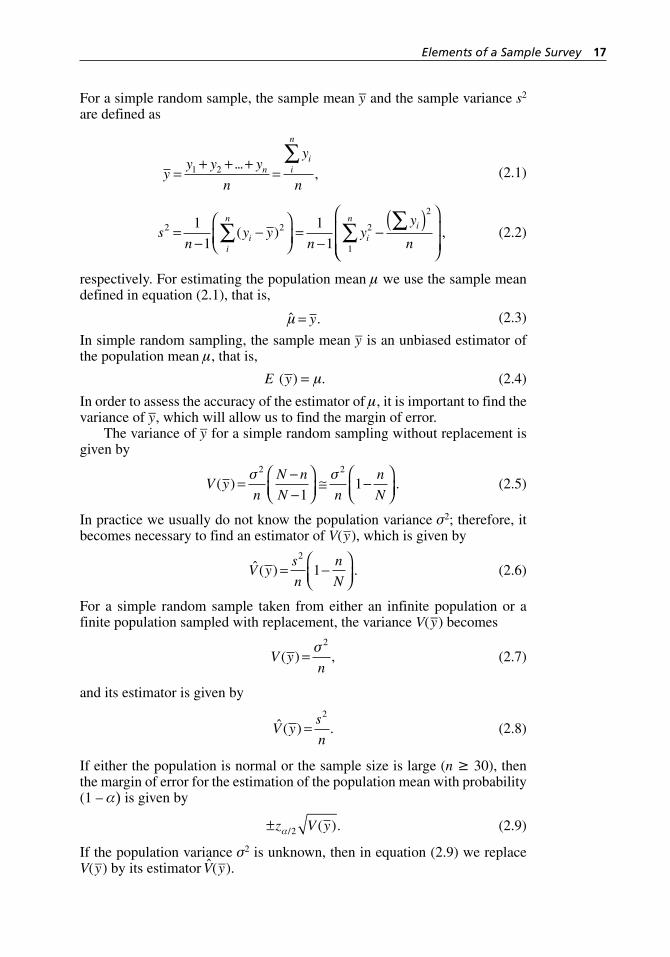
Elements of a Sample Survey 17
For a simple random sample, the sample mean y– and the sample variance s2 are defined as
y
y y y
n
y
nn
ii
n
=+ + +
=∑
1 2 ...,
(2.1)
sn
y yn
yy
nii
n
i
ni2 2 2
1
2
1
1
1
1=
−−
⎛
⎝⎜⎞
⎠⎟=
−−
( )⎛∑ ∑ ∑
( )⎝⎝⎜⎜
⎞
⎠⎟⎟
,
(2.2)
respectively. For estimating the population mean µ we use the sample mean defined in equation (2.1), that is,
ˆ .µ = y (2.3)
In simple random sampling, the sample mean y– is an unbiased estimator of the population mean µ, that is,
E ( ) .y = µ (2.4)
In order to assess the accuracy of the estimator of µ, it is important to find the variance of y–, which will allow us to find the margin of error.
The variance of y– for a simple random sampling without replacement is given by
V y
n
N n
N n
n
N( ) .=
−−
⎛⎝⎜
⎞⎠⎟
≅ −⎛⎝⎜
⎞⎠⎟
σ σ2 2
11
(2.5)
In practice we usually do not know the population variance σ2; therefore, it becomes necessary to find an estimator of V(y–), which is given by
ˆ ( ) .V ys
n
n
N= −
⎛⎝⎜
⎞⎠⎟
2
1
(2.6)
For a simple random sample taken from either an infinite population or a finite population sampled with replacement, the variance V(y–) becomes
V y
n( ) ,=
σ2
(2.7)
and its estimator is given by
ˆ ( ) .V y
s
n=
2
(2.8)
If either the population is normal or the sample size is large (n ≥ 30), then the margin of error for the estimation of the population mean with probability (1 – α) is given by
±z V yα/ ( ).2 (2.9)
If the population variance σ2 is unknown, then in equation (2.9) we replace V(y–) by its estimator V(y–).
H1277 ch02.indd 17H1277 ch02.indd 17 3/8/07 5:31:10 PM3/8/07 5:31:10 PM
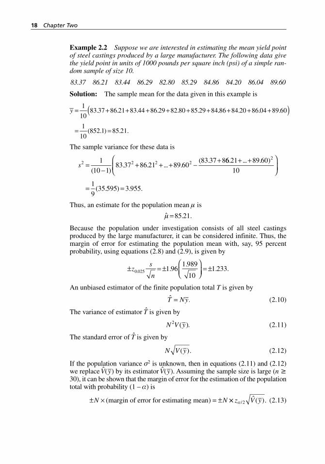
18 Chapter Two
Example 2.2 Suppose we are interested in estimating the mean yield point of steel castings produced by a large manufacturer. The following data give the yield point in units of 1000 pounds per square inch (psi) of a simple ran-dom sample of size 10.
83.37 86.21 83.44 86.29 82.80 85.29 84.86 84.20 86.04 89.60
Solution: The sample mean for the data given in this example is
y = + + + + + +1
1083 37 86 21 83 44 86 29 82 80 85 29 84. . . . . . .. . . .
( . ) . .
86 84 20 86 04 89 60
1
10852 1 85 21
+ + +
= =
( )
The sample variance for these data is
s2 2 2 21
10 183 37 86 21 89 60
83 37 8=
−+ + + −
+( )
. . ... .( . 66 21 89 60
10
1
935 595 3 955
2. ... . )
( . ) . .
+ +⎛
⎝⎜⎞
⎠⎟
= =
Thus, an estimate for the population mean µ is
ˆ . .µ = 85 21
Because the population under investigation consists of all steel castings produced by the large manufacturer, it can be considered infinite. Thus, the margin of error for estimating the population mean with, say, 95 percent probability, using equations (2.8) and (2.9), is given by
± = ±
⎛⎝⎜
⎞⎠⎟
= ±zs
n0 025 1 96
1 989
101 233. .
.. .
An unbiased estimator of the finite population total T is given by
ˆ .T Ny= (2.10)
The variance of estimator T is given by
N V y2 ( ). (2.11)
The standard error of T is given by
N V y( ). (2.12)
If the population variance σ2 is unknown, then in equations (2.11) and (2.12) we replace V(y–) by its estimator V(y–). Assuming the sample size is large (n ≥ 30), it can be shown that the margin of error for the estimation of the population total with probability (1 – α) is
± × = ±N N( )margin of error for estimating mean ×× z V yα/ˆ ( ).2 (2.13)
H1277 ch02.indd 18H1277 ch02.indd 18 3/8/07 5:31:11 PM3/8/07 5:31:11 PM
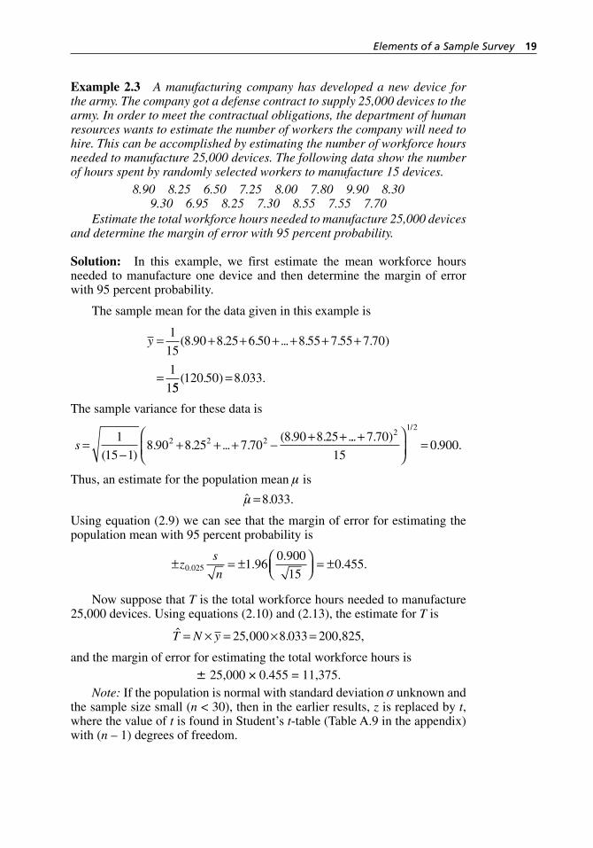
Elements of a Sample Survey 19
Example 2.3 A manufacturing company has developed a new device for the army. The company got a defense contract to supply 25,000 devices to the army. In order to meet the contractual obligations, the department of human resources wants to estimate the number of workers the company will need to hire. This can be accomplished by estimating the number of workforce hours needed to manufacture 25,000 devices. The following data show the number of hours spent by randomly selected workers to manufacture 15 devices.
8.90 8.25 6.50 7.25 8.00 7.80 9.90 8.309.30 6.95 8.25 7.30 8.55 7.55 7.70
Estimate the total workforce hours needed to manufacture 25,000 devices and determine the margin of error with 95 percent probability.
Solution: In this example, we first estimate the mean workforce hours needed to manufacture one device and then determine the margin of error with 95 percent probability.
The sample mean for the data given in this example is
y = + + + + + +
=
1
158 90 8 25 6 50 8 55 7 55 7 70
1
1
( . . . ... . . . )
55120 50 8 033( . ) . .=
The sample variance for these data is
s =−
+ + + −+ +1
15 18 90 8 25 7 70
8 90 8 252 2 2
( ). . ... .
( . . .... . ). .
/+⎛
⎝⎜⎞
⎠⎟=
7 70
150 900
21 2
Thus, an estimate for the population mean µ is
ˆ . .µ = 8 033
Using equation (2.9) we can see that the margin of error for estimating the population mean with 95 percent probability is
± = ± ⎛⎝⎜
⎞⎠⎟ = ±z
s
n0 025 1 96
0 900
150 455. .
.. .
Now suppose that T is the total workforce hours needed to manufacture 25,000 devices. Using equations (2.10) and (2.13), the estimate for T is
ˆ , . , ,T N y= × = × =25 000 8 033 200 825
and the margin of error for estimating the total workforce hours is ± 25,000 × 0.455 = 11,375.
Note: If the population is normal with standard deviation σ unknown and the sample size small (n < 30), then in the earlier results, z is replaced by t, where the value of t is found in Student’s t-table (Table A.9 in the appendix) with (n – 1) degrees of freedom.
H1277 ch02.indd 19H1277 ch02.indd 19 3/8/07 5:31:11 PM3/8/07 5:31:11 PM
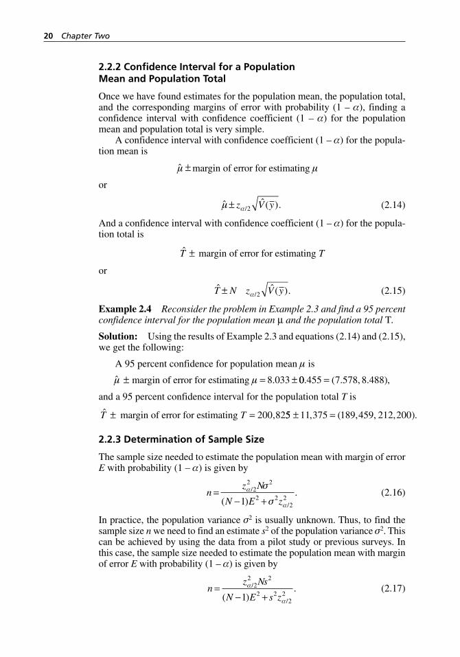
20 Chapter Two
2.2.2 Confidence Interval for a Population Mean and Population Total
Once we have found estimates for the population mean, the population total, and the corresponding margins of error with probability (1 – α), finding a confidence interval with confidence coefficient (1 – α) for the population mean and population total is very simple.
A confidence interval with confidence coefficient (1 – α) for the popula-tion mean is
ˆ margin of error for estimating
or
ˆ ˆ ( )./z V y2 (2.14)
And a confidence interval with confidence coefficient (1 – α) for the popula-tion total is
T Tmargin of error for estimating
or
ˆ ˆ ( )./T N z V y2 (2.15)
Example 2.4 Reconsider the problem in Example 2.3 and find a 95 percent confidence interval for the population mean µ and the population total T.
Solution: Using the results of Example 2.3 and equations (2.14) and (2.15), we get the following:
A 95 percent confidence for population mean µ is
ˆ .margin of error for estimating 8 033 00 455 7 578 8 488. ( . , . ),
and a 95 percent confidence interval for the population total T is
ˆ ,T Tmargin of error for estimating 200 8255 11 375 189 459 212 200, ( , , , ).
2.2.3 Determination of Sample Size
The sample size needed to estimate the population mean with margin of error E with probability (1 – α) is given by
n
z N
N E z=
− +α
α
σ
σ/
/( ).2
2 2
2 22
21 (2.16)
In practice, the population variance σ2 is usually unknown. Thus, to find the sample size n we need to find an estimate s2 of the population variance σ2. This can be achieved by using the data from a pilot study or previous surveys. In this case, the sample size needed to estimate the population mean with margin of error E with probability (1 – α) is given by
n
z Ns
N E s z=
− +α
α
/
/( ).2
2 2
2 22
21 (2.17)
H1277 ch02.indd 20H1277 ch02.indd 20 3/8/07 5:31:11 PM3/8/07 5:31:11 PM
Elements of a Sample Survey 21
If the population size N is large, then the factor (N – 1) in equation (2.17) is usually replaced by N.
Note: The sample size needed to estimate the population total with mar-gin of error E′ with probability (1 – α) can be found by using equation (2.16) or (2.17) depending on whether the population variance σ2 is known and replacing E with (E′/N).
Example 2.5 Suppose in Example 2.3 we would like the margin of error for estimating the population mean to be 0.25 with probability 0.99. Determine the appropriate sample size to achieve this goal.
Solution: From the information provided to us, we have
E z= =0 25 2 5752. , . ,/α
and from Example 2.3, we have N = 25,000 and s = 0.900.Plugging these values into equation (2.17) and replacing the factor (N – 1) in the denominator by N, we get
n = × ×+
( . ) ( , ) ( . )
, ( . ) (
2 575 25 000 0 900
25 000 0 25
2 2
2 00 900 2 575
86
2 2. ) ( . )
.≅
Note that the sample size for estimating the population total with margin of error 6250 (= 25,000 × 0.25) is again equal to 86. To attain a sample of size 86, we take another simple random sample of size 71, which is usually known as a supplemental sample, and then combine this sample with the one that we had already taken, which was of size 15.
2.3 Stratified Random Sampling
It is not uncommon in a manufacturing process for a characteristic of inter-est to vary from country to country, region to region, plant to plant, or machine to machine. For example, a Six Sigma Green Belt might be inter-ested in finding the longevity of parts manufactured in different regions of the United States. Clearly, the longevity of such parts may vary from region to region depending on where the parts are manufactured. This could be due to differences in raw materials, training of the workers, or differences in machines. In such cases where the population is heterogeneous, we get more precise estimates by using a sample design known as stratified ran-dom sampling. In stratified random sampling, the population is divided into different nonoverlapping groups, called strata, such that they consti-tute the whole population; the population is as homogeneous as possible within each stratum but varies between strata. Then a stratified random sample is taken by selecting a simple random sample from each stratum.
Some of the advantages of stratified random sampling over simple ran-dom sampling are as follows:
H1277 ch02.indd 21H1277 ch02.indd 21 3/8/07 5:31:12 PM3/8/07 5:31:12 PM
22 Chapter Two
1. It provides more precise estimates for population parameters than simple random sampling would provide with the same sample size.
2. A stratified sample is more convenient to administer, which may result in a lower cost for sampling.
3. It provides a simple random sample for each subgroup or stratum, which are homogeneous. Therefore, these samples can prove to be very useful for studying each individual subgroup separately without incurring any extra cost.
Before we look into how to use the information obtained from a stratified random sample to estimate population parameters, we will briefly discuss the process of generating a stratified random sample:
Divide the sampling population of N units into nonoverlapping sub-populations or strata of N1, N2, . . . , NK units, respectively. These strata constitute the whole population of N units. That is, N = N1 + N2 + . . . +NK.
Select independently from each stratum a simple random sample of size n1, n2, . . . , nK so that n = n1 + n2 + . . . + nK is the total sample size.
To make full use of stratification, the strata sizes N1, N2, . . . , NK must be known.
2.3.1 Estimation of a Population Mean and Population Total
Let y y y y y y y yN N K11 12 1 21 22 2 11 2, , . . . , ; , , . . . , ; . . .; , KK KNy K2,... , be the sampling units in 1, 2, . . . , Kth stratum, respectively, and let y y y y y yn n11 12 1 21 22 21 2, , . . . , ; , , . . . , ; ...; , , ...,y y yK K KnK1 2 be the simple random samples of sizes n1, n2, . . . , nK from them, respectively. Let µ and T be the population mean and population total, respectively, and let µi, Ti, σ i
2 be the population mean, total, and vari-ance of the ith stratum, respectively. Then, we have
T T Ni
i
K
i ii
K
= == =∑ ∑
1 1
µ ,
(2.18)
µ µ= =
=∑T N
NNi i
i
K1
1
.
(2.19)
Let y–i be the sample mean of the simple random sample from the ith stratum. From the previous section we know that y–i is an unbiased estimator of the mean µi of the ith stratum. An unbiased estimator of the population mean µ, which we denote as y–st, is given by
ˆ ,µ = =
=∑y
NN yst i i
i
K1
1 (2.20)
•
•
•
H1277 ch02.indd 22H1277 ch02.indd 22 3/8/07 5:31:12 PM3/8/07 5:31:12 PM
Elements of a Sample Survey 23
where
y
nyi
iij
j
ni
==
∑1
1
.
(2.21)
An estimator of the population total T is given by
ˆ ˆ ˆ .T T N N y N yii
K
i ii
K
i ii
K
st= = = = ×= = =∑ ∑ ∑
1 1 1
µ
(2.22)
Recall that from equation (2.5) we have
V y
n
N n
Nii
i
i i
i
( ) .=−−
⎛⎝⎜
⎞⎠⎟
σ2
1
(2.23)
From equations (2.20) and (2.23), it follows that the variance of the estimator y–st of the population mean µ is given by
V yN
N V y
NN
n
N n
N
st i ii
K
ii
i
i i
i
( ) ( )=
=−−
=∑1
1
22
1
22
2σ
111
⎛⎝⎜
⎞⎠⎟=
∑i
K
.
(2.24)
An estimator of the variance in equation (2.24) is given by
ˆ ( ) .V yN
Ns
n
n
Nst ii
i
i
ii
K
= −⎛⎝⎜
⎞⎠⎟=
∑11
22
2
1 (2.25)
From equations (2.22) and (2.25), it follows that the variance of the estimator of the population total T is given by
V T N V y
Nn
N n
N
st
ii
i
i i
ii
K
( ˆ) ( )=
=−−
⎛⎝⎜
⎞⎠⎟=
∑
2
22
1 1
σ..
(2.26)
An estimator of the variance in equation (2.26) is given by
ˆ ( ˆ) ˆ ( )
.
V T N V y
Ns
n
n
N
st
ii
i
i
ii
K
=
= −⎛⎝⎜
⎞⎠⎟=
∑
2
22
1
1
(2.27)
If either the population is normal or the sample size is large (n ≥ 30), then the margin of error for the estimation of the population mean with probability (1 – α) is given by
± = ±−−
⎛⎝⎜
⎞⎠⎟
z V y zN
Nn
N n
Nst ii
i
i i
iiα α
σ/ /( )2 2
221
1==∑
1
K
.
(2.28)
H1277 ch02.indd 23H1277 ch02.indd 23 3/8/07 5:31:12 PM3/8/07 5:31:12 PM
24 Chapter Two
When the strata variances are unknown, which is usually the case, the stra-tum variance σ i
2 in equation (2.28) is replaced by its estimator si2 . Then the
margin of error for the estimation of the population mean with probability (1 – α) is given by
± −⎛⎝⎜
⎞⎠⎟=
∑zN
Ns
n
n
Nii
i
i
ii
K
α/ .22
2
1
11
(2.29)
The margin of error for the estimation of the population total with probability (1 – α) is given by
±−−
⎛⎝⎜
⎞⎠⎟=
∑z Nn
N n
Nii
i
i i
ii
K
α
σ/ .2
22
1 1
(2.30)
Again, when the strata variances are unknown, the stratum variance σ i2 in
equation (2.30) is replaced by its estimator si2 . Then the margin of error for
the estimation of the population total with probability (1 – α) is given by
± −⎛⎝⎜
⎞⎠⎟=
∑z Ns
n
n
Nii
i
i
ii
K
α/ .22
2
1
1
(2.31)
2.3.2 Confidence Interval for a Population Mean and Population Total
From equations (2.29) and (2.31) we have the margins of error for estimating the population mean and population total with probability (1 – α). A confi-dence interval with confidence coefficient (1 – α) for the population mean and population total is given by
ˆ /µ α± −⎛⎝⎜
⎞⎠⎟=
∑zN
Ns
n
n
Nii
i
i
ii
K
22
2
1
11
(2.32)
and
ˆ ,/T z Ns
n
n
Nii
i
i
ii
K
± −⎛⎝⎜
⎞⎠⎟=
∑α 22
2
1
1
(2.33)
respectively.
Notes
1. An estimate y– of the population mean obtained from a simple random sample coincides with estimate y–st obtained from a stratified random sample if in every stratum ni/Ni is equal to n/N.
2. If the sample size in every stratum relative to the stratum size is small (ni /Ni < 5%), then the factor ni/Ni in equations (2.25) through (2.33) is usually ignored.
H1277 ch02.indd 24H1277 ch02.indd 24 3/8/07 5:31:12 PM3/8/07 5:31:12 PM
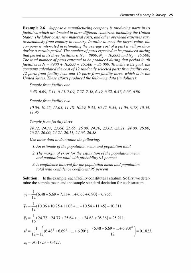
Elements of a Sample Survey 25
Example 2.6 Suppose a manufacturing company is producing parts in its facilities, which are located in three different countries, including the United States. The labor costs, raw material costs, and other overhead expenses vary tremendously from country to country. In order to meet the target value, the company is interested in estimating the average cost of a part it will produce during a certain period. The number of parts expected to be produced during that period in its three facilities is N1 = 8900, N2 = 10,600, and N3 = 15,500. The total number of parts expected to be produced during that period in all facilities is N = 8900 + 10,600 + 15,500 = 35,000. To achieve its goal, the company calculated the cost of 12 randomly selected parts from facility one, 12 parts from facility two, and 16 parts from facility three, which is in the United States. These efforts produced the following data (in dollars):
Sample from facility one
6.48, 6.69, 7.11, 6.15, 7.09, 7.27, 7.58, 6.49, 6.32, 6.47, 6.63, 6.90
Sample from facility two
10.06, 10.25, 11.03, 11.18, 10.29, 9.33, 10.42, 9.34, 11.06, 9.78, 10.54, 11.45
Sample from facility three
24.72, 24.77, 25.64, 25.65, 26.09, 24.70, 25.05, 23.21, 24.00, 26.00, 26.21, 26.00, 24.21, 26.11, 24.63, 26.38
Use these data to determine the following:
1. An estimate of the population mean and population total
2. The margin of error for the estimation of the population mean and population total with probability 95 percent
3. A confidence interval for the population mean and population total with confidence coefficient 95 percent
Solution: In the example, each facility constitutes a stratum. So first we deter-mine the sample mean and the sample standard deviation for each stratum.
y11
126 48 6 69 7 11 6 63 6 90 6 765= + + + + +( ) =. . . ... . . . ,
yy21
1210 06 10 25 11 03 10 54 11 45= + + + + +( ) =. . . ... . . 110 311
1
1624 72 24 77 25 64 24 63 23
. ,
. . . ... .y = + + + + + 66 38 25 211
1
12 16 48 6 69 61
2 2 2
. . ,
( . . ... .
( ) =
=−
+ + +s 9906 48 6 69 6 90
120 18232
2
)( . . ... . )
. ,− + + +⎛⎝⎜
⎞⎠⎟
=
ss1 0 1823 0 427= =. . ,
H1277 ch02.indd 25H1277 ch02.indd 25 3/8/07 5:31:12 PM3/8/07 5:31:12 PM
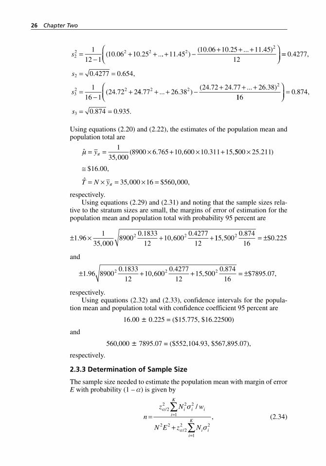
26 Chapter Two
s22 2 21
12 110 06 10 25=
−+ +( . . .... . )
( . . ... . )+ − + + +⎛⎝⎜
⎞⎠⎟
11 4510 06 10 25 11 45
122
2
==
= =
=−
+
0 4277
0 4277 0 654
1
16 124 72 2
2
32 2
. ,
. . ,
( .
s
s 44 77 26 3824 72 24 77 26 382 2
2
. ... . )( . . ... . )+ + − + + +
1160 874
0 874 0 9353
⎛⎝⎜
⎞⎠⎟
=
= =
. ,
. . .s
Using equations (2.20) and (2.22), the estimates of the population mean and population total are
ˆ,
( . , . ,µ = = × + × +yst1
35 0008900 6 765 10 600 10 311 15 5500 25 211
16 00
35 000 16 560
×
≅
= × = × =
. )
$ . ,
ˆ , $T N yst ,, ,000
respectively.Using equations (2.29) and (2.31) and noting that the sample sizes rela-
tive to the stratum sizes are small, the margins of error of estimation for the population mean and population total with probability 95 percent are
± × + +1 96
1
35 0008900
0 1833
1210 600
0 4277
122 2.
,
.,
.115 500
0 874
160 2252,
.$ .= ±
and
± + +1 96 8900
0 1833
1210 600
0 4277
1215 500
02 2 2..
,.
,..
$ . ,874
167895 07= ±
respectively.Using equations (2.32) and (2.33), confidence intervals for the popula-
tion mean and population total with confidence coefficient 95 percent are
16.00 ± 0.225 = ($15.775, $16.22500)
and
560,000 ± 7895.07 = ($552,104.93, $567,895.07),
respectively.
2.3.3 Determination of Sample Size
The sample size needed to estimate the population mean with margin of error E with probability (1 – α) is given by
n
z N w
N E z N
i i ii
K
i ii
K=
+
=
=
∑
∑
α
α
σ
σ
/
/
/
,2
2 2 2
1
2 22
2 2
1
(2.34)
H1277 ch02.indd 26H1277 ch02.indd 26 3/8/07 5:31:12 PM3/8/07 5:31:12 PM
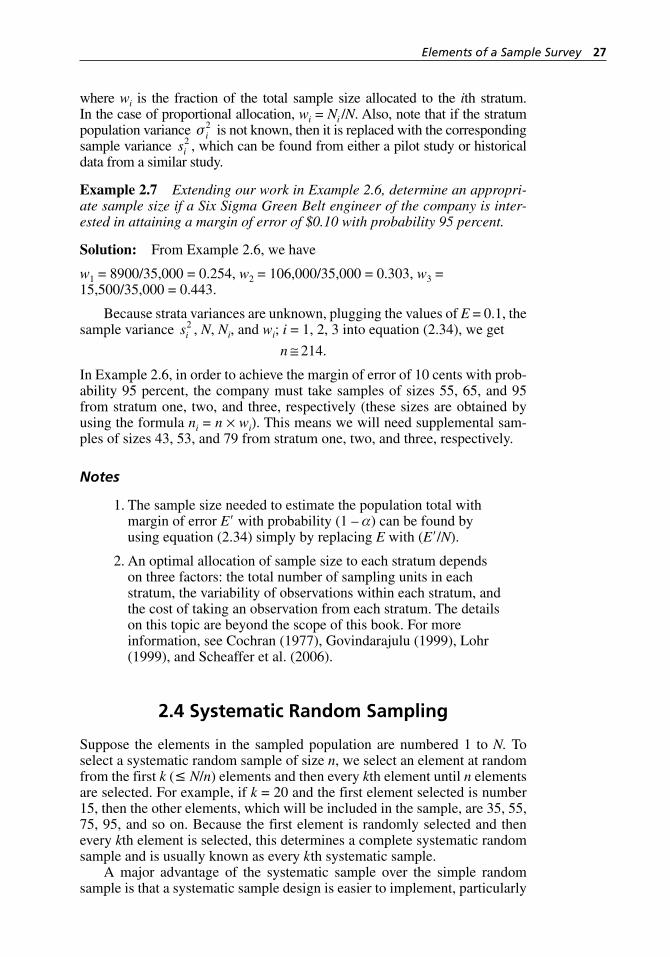
Elements of a Sample Survey 27
where wi is the fraction of the total sample size allocated to the ith stratum. In the case of proportional allocation, wi = Ni /N. Also, note that if the stratum population variance σ i
2 is not known, then it is replaced with the corresponding sample variance si
2 , which can be found from either a pilot study or historical data from a similar study.
Example 2.7 Extending our work in Example 2.6, determine an appropri-ate sample size if a Six Sigma Green Belt engineer of the company is inter-ested in attaining a margin of error of $0.10 with probability 95 percent.
Solution: From Example 2.6, we have
w1 = 8900/35,000 = 0.254, w2 = 106,000/35,000 = 0.303, w3 = 15,500/35,000 = 0.443.
Because strata variances are unknown, plugging the values of E = 0.1, the sample variance si
2 , N, Ni, and wi; i = 1, 2, 3 into equation (2.34), we get
n ≅ 214.
In Example 2.6, in order to achieve the margin of error of 10 cents with prob-ability 95 percent, the company must take samples of sizes 55, 65, and 95 from stratum one, two, and three, respectively (these sizes are obtained by using the formula ni = n × wi). This means we will need supplemental sam-ples of sizes 43, 53, and 79 from stratum one, two, and three, respectively.
Notes
1. The sample size needed to estimate the population total with margin of error E′ with probability (1 – α) can be found by using equation (2.34) simply by replacing E with (E′/N).
2. An optimal allocation of sample size to each stratum depends on three factors: the total number of sampling units in each stratum, the variability of observations within each stratum, and the cost of taking an observation from each stratum. The details on this topic are beyond the scope of this book. For more information, see Cochran (1977), Govindarajulu (1999), Lohr (1999), and Scheaffer et al. (2006).
2.4 Systematic Random Sampling
Suppose the elements in the sampled population are numbered 1 to N. To select a systematic random sample of size n, we select an element at random from the first k (≤ N/n) elements and then every kth element until n elements are selected. For example, if k = 20 and the first element selected is number 15, then the other elements, which will be included in the sample, are 35, 55, 75, 95, and so on. Because the first element is randomly selected and then every kth element is selected, this determines a complete systematic random sample and is usually known as every kth systematic sample.
A major advantage of the systematic sample over the simple random sample is that a systematic sample design is easier to implement, particularly
H1277 ch02.indd 27H1277 ch02.indd 27 3/8/07 5:31:13 PM3/8/07 5:31:13 PM
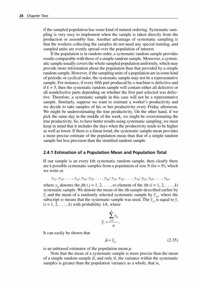
28 Chapter Two
if the sampled population has some kind of natural ordering. Systematic sam-pling is very easy to implement when the sample is taken directly from the production or assembly line. Another advantage of systematic sampling is that the workers collecting the samples do not need any special training, and sampled units are evenly spread over the population of interest.
If the population is in random order, a systematic random sample provides results comparable with those of a simple random sample. Moreover, a system-atic sample usually covers the whole sampled population uniformly, which may provide more information about the population than that provided by a simple random sample. However, if the sampling units of a population are in some kind of periodic or cyclical order, the systematic sample may not be a representative sample. For instance, if every fifth part produced by a machine is defective and if k = 5, then the systematic random sample will contain either all defective or all nondefective parts depending on whether the first part selected was defec-tive. Therefore, a systematic sample in this case will not be a representative sample. Similarly, suppose we want to estimate a worker’s productivity and we decide to take samples of his or her productivity every Friday afternoon. We might be underestimating the true productivity. On the other hand, if we pick the same day in the middle of the week, we might be overestimating the true productivity. So, to have better results using systematic sampling, we must keep in mind that it includes the days when the productivity tends to be higher as well as lower. If there is a linear trend, the systematic sample mean provides a more precise estimate of the population mean than that of a simple random sample but less precision than the stratified random sample.
2.4.1 Estimation of a Population Mean and Population Total
If our sample is an every kth systematic random sample, then clearly there are k possible systematic samples from a population of size N (kn = N), which we write as
y11, y12, . . . , y1n; y21, y22, . . . , y2n; y31, y32, . . . , y3n; yk1, yk2, . . . , ykn,
where yij denotes the jth ( j = 1, 2, . . . , n) element of the ith (i = 1, 2, . . . , k) systematic sample. We denote the mean of the ith sample described earlier by y–i and the mean of a randomly selected systematic sample by y–sy, where the subscript sy means that the systematic sample was used. The y–sy is equal to y–i (i = 1, 2, . . . , k) with probability 1/k, where
y
y
ni
ijj
n
= =∑
1 .
It can easily be shown that
µ = ysy
(2.35)
is an unbiased estimator of the population mean µ.Note that the mean of a systematic sample is more precise than the mean
of a simple random sample if, and only if, the variance within the systematic samples is greater than the population variance as a whole, that is,
H1277 ch02.indd 28H1277 ch02.indd 28 3/8/07 5:31:13 PM3/8/07 5:31:13 PM
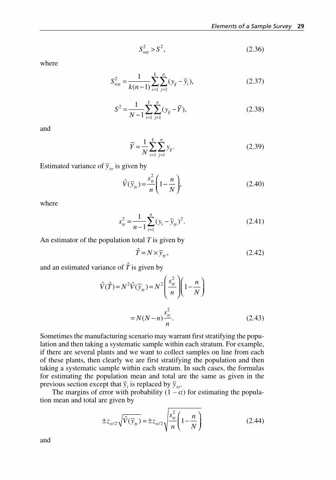
Elements of a Sample Survey 29
S Swsy
2 2> ,
(2.36)
where
S
k ny ywsy ij i
j
n
i
k2
11
1
1=
−−
==∑∑( )
( ),
(2.37)
S
Ny Yij
j
n
i
k2
11
1
1=
−−
==∑∑ ( ),
(2.38)
and
Y
Nyij
j
n
i
k
===
∑∑1
11
.
(2.39)
Estimated variance of y–sy is given by
ˆ ( ) ,V ys
n
n
Nsysy= −
⎛⎝⎜
⎞⎠⎟
2
1
(2.40)
where
s
ny ysy i sy
i
n2 2
1
1
1=
−−
=∑( ) .
(2.41)
An estimator of the population total T is given by
ˆ ,T N ysy= ×
(2.42)
and an estimated variance of T is given by
ˆ ( ˆ) ˆ ( )V T N V y Ns
n
n
Nsysy= =
⎛
⎝⎜
⎞
⎠⎟ −
⎛⎝⎜
⎞⎠⎟
2 22
1
= −N N n
s
nsy( ) .2
(2.43)
Sometimes the manufacturing scenario may warrant first stratifying the popu-lation and then taking a systematic sample within each stratum. For example, if there are several plants and we want to collect samples on line from each of these plants, then clearly we are first stratifying the population and then taking a systematic sample within each stratum. In such cases, the formulas for estimating the population mean and total are the same as given in the previous section except that y–i is replaced by y–sy.
The margins of error with probability (1 – α) for estimating the popula-tion mean and total are given by
± = ± −
⎛⎝⎜
⎞⎠⎟
z V y zs
n
n
Nsysy
α α/ /ˆ ( )2 2
2
1
(2.44)
and
H1277 ch02.indd 29H1277 ch02.indd 29 3/8/07 5:31:13 PM3/8/07 5:31:13 PM
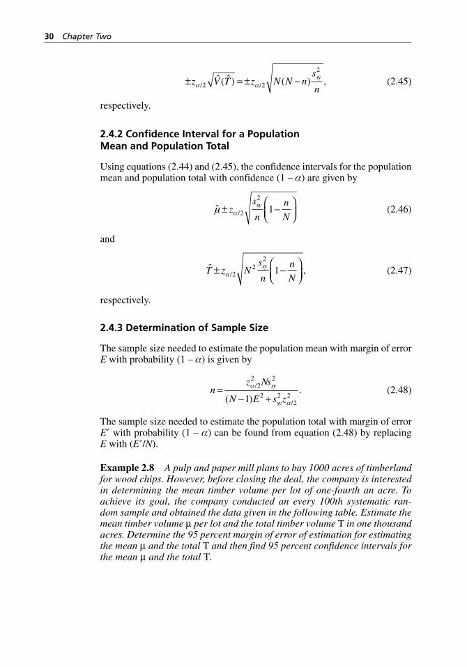
30 Chapter Two
± = ± −z V T z N N n
s
nsy
α α/ /ˆ ( ˆ) ( ) ,2 2
2
(2.45)
respectively.
2.4.2 Confidence Interval for a Population Mean and Population Total
Using equations (2.44) and (2.45), the confidence intervals for the population mean and population total with confidence (1 – α) are given by
ˆ /µ α± −⎛⎝⎜
⎞⎠⎟
zs
n
n
Nsy
2
2
1
(2.46)
and
ˆ ,/T z Ns
n
n
Nsy± −
⎛⎝⎜
⎞⎠⎟α 2
22
1
(2.47)
respectively.
2.4.3 Determination of Sample Size
The sample size needed to estimate the population mean with margin of error E with probability (1 – α) is given by
nz Ns
N E s z
sy
sy
=− +
α
α
/
/( ).2
2 2
2 22
21
(2.48)
The sample size needed to estimate the population total with margin of error E′ with probability (1 – α) can be found from equation (2.48) by replacing E with (E′/N).
Example 2.8 A pulp and paper mill plans to buy 1000 acres of timberland for wood chips. However, before closing the deal, the company is interested in determining the mean timber volume per lot of one- fourth an acre. To achieve its goal, the company conducted an every 100th systematic ran-dom sample and obtained the data given in the following table. Estimate the mean timber volume µ per lot and the total timber volume T in one thousand acres. Determine the 95 percent margin of error of estimation for estimating the mean µ and the total T and then find 95 percent confidence intervals for the mean µ and the total T.
H1277 ch02.indd 30H1277 ch02.indd 30 3/8/07 5:31:13 PM3/8/07 5:31:13 PM
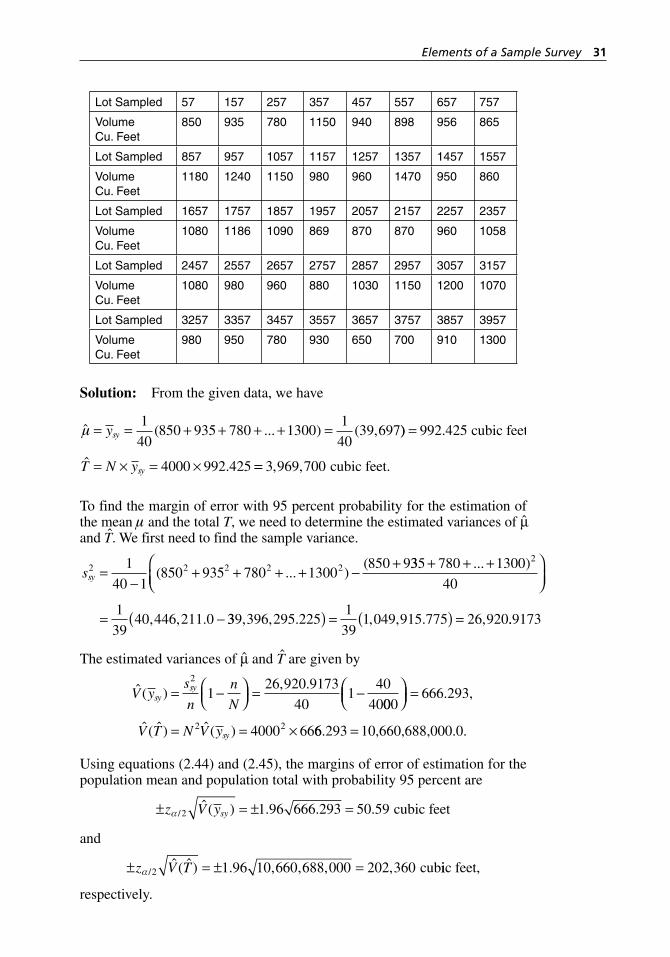
Elements of a Sample Survey 31
Lot Sampled 57 157 257 357 457 557 657 757
Volume Cu. Feet
850 935 780 1150 940 898 956 865
Lot Sampled 857 957 1057 1157 1257 1357 1457 1557
Volume Cu. Feet
1180 1240 1150 980 960 1470 950 860
Lot Sampled 1657 1757 1857 1957 2057 2157 2257 2357
Volume Cu. Feet
1080 1186 1090 869 870 870 960 1058
Lot Sampled 2457 2557 2657 2757 2857 2957 3057 3157
Volume Cu. Feet
1080 980 960 880 1030 1150 1200 1070
Lot Sampled 3257 3357 3457 3557 3657 3757 3857 3957
Volume Cu. Feet
980 950 780 930 650 700 910 1300
Solution: From the given data, we have
ˆ ( ... ) ( ,µ = = + + + + =ysy1
40850 935 780 1300
1
4039 697)) .
ˆ .
=
= × = ×
992 425
4000 992 425
cubic feet
T N ysy == 3 969 700, , cubic feet.
To find the margin of error with 95 percent probability for the estimation of the mean µ and the total T, we need to determine the estimated variances of µ and T. We first need to find the sample variance.
ssy2 2 2 2 21
40 1850 935 780 1300
850 9=−
+ + + + − +( ... )
( 335 780 1300
40
1
3940 446 211 0
2+ + +⎛⎝⎜
⎞⎠⎟
= −
... )
, , . 339 396 295 2251
391 049 915 775 26 920, , . , , . ,( ) = ( ) = ..9173
The estimated variances of µ and T are given by
ˆ ( ), .
V ys
n
n
Nsy
sy= −⎛⎝⎜
⎞⎠⎟ = −
2
126 920 9173
401
40
40000
4000 662 2
⎛⎝⎜
⎞⎠⎟ =
= = ×
666.293,
ˆ ( ˆ) ˆ ( )V T N V ysy 66 293. = 10,660,688,000.0.
Using equations (2.44) and (2.45), the margins of error of estimation for the population mean and population total with probability 95 percent are
± = ± =z V ysyα /
ˆ ( ) . . .2 1 96 666 293 50 59 cubic feet
and
± = ± =z V Tα/ˆ ( ˆ) . , , , ,2 1 96 10 660 688 000 202 360 cubiic feet,
respectively.
H1277 ch02.indd 31H1277 ch02.indd 31 3/8/07 5:31:13 PM3/8/07 5:31:13 PM
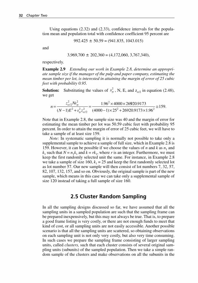
32 Chapter Two
Using equations (2.32) and (2.33), confidence intervals for the popula-tion mean and population total with confidence coefficient 95 percent are
992.425 ± 50.59 = (941.835, 1043.015)
and
3,969,700 ± 202,360 = (4,172,060, 3,767,340),
respectively.
Example 2.9 Extending our work in Example 2.8, determine an appropri-ate sample size if the manager of the pulp and paper company, estimating the mean timber per lot, is interested in attaining the margin of error of 25 cubic feet with probability 0.95.
Solution: Substituting the values of ssy2 , N, E, and zα/2 in equation (2.48),
we get
nz Ns
N E s z
sy
sy
=− +
=× ×α
α
/
/( )
.22 2
2 22
2
2
1
1 96 4000 269920 9173
4000 1 25 26920 9173 1 96159
2 2
.
( ) . ..
− × + ×≅
Note that in Example 2.8, the sample size was 40 and the margin of error for estimating the mean timber per lot was 50.59 cubic feet with probability 95 percent. In order to attain the margin of error of 25 cubic feet, we will have to take a sample of at least size 159.
Note: In systematic sampling it is normally not possible to take only a supplemental sample to achieve a sample of full size, which in Example 2.8 is 159. However, it can be possible if we choose the values of n and k as n1 and k1 such that N = n1k1 and k = rk1, where r is an integer. Furthermore, we must keep the first randomly selected unit the same. For instance, in Example 2.8 we take a sample of size 160, k1 = 25 and keep the first randomly selected lot as lot number 57. Our new sample will then consist of lot numbers 7, 32, 57, 82, 107, 132, 157, and so on. Obviously, the original sample is part of the new sample, which means in this case we can take only a supplemental sample of size 120 instead of taking a full sample of size 160.
2.5 Cluster Random Sampling
In all the sampling designs discussed so far, we have assumed that all the sampling units in a sampled population are such that the sampling frame can be prepared inexpensively, but this may not always be true. That is, to prepare a good frame listing is very costly, or there are not enough funds to meet that kind of cost, or all sampling units are not easily accessible. Another possible scenario is that all the sampling units are scattered, so obtaining observations on each sampling unit is not only very costly, but also very time consuming. In such cases we prepare the sampling frame consisting of larger sampling units, called clusters, such that each cluster consists of several original sam-pling units (subunits) of the sampled population. Then we take a simple ran-dom sample of the clusters and make observations on all the subunits in the
H1277 ch02.indd 32H1277 ch02.indd 32 3/8/07 5:31:14 PM3/8/07 5:31:14 PM
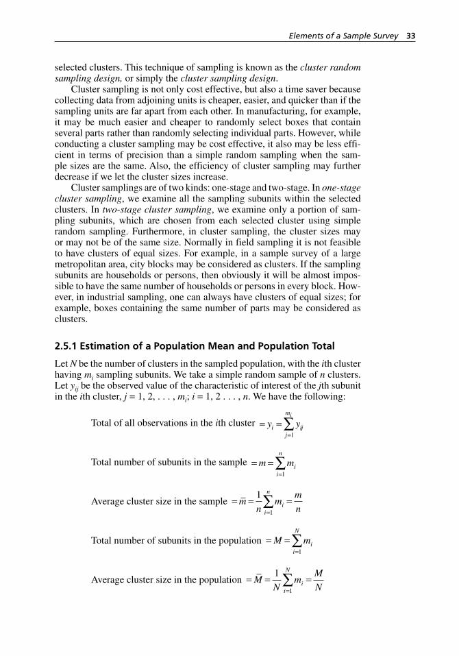
Elements of a Sample Survey 33
selected clusters. This technique of sampling is known as the cluster random sampling design, or simply the cluster sampling design.
Cluster sampling is not only cost effective, but also a time saver because collecting data from adjoining units is cheaper, easier, and quicker than if the sampling units are far apart from each other. In manufacturing, for example, it may be much easier and cheaper to randomly select boxes that contain several parts rather than randomly selecting individual parts. However, while conducting a cluster sampling may be cost effective, it also may be less effi-cient in terms of precision than a simple random sampling when the sam-ple sizes are the same. Also, the efficiency of cluster sampling may further decrease if we let the cluster sizes increase.
Cluster samplings are of two kinds: one- stage and two- stage. In one-stage cluster sampling, we examine all the sampling subunits within the selected clusters. In two-stage cluster sampling, we examine only a portion of sam-pling subunits, which are chosen from each selected cluster using simple random sampling. Furthermore, in cluster sampling, the cluster sizes may or may not be of the same size. Normally in field sampling it is not feasible to have clusters of equal sizes. For example, in a sample survey of a large metropolitan area, city blocks may be considered as clusters. If the sampling subunits are households or persons, then obviously it will be almost impos-sible to have the same number of households or persons in every block. How-ever, in industrial sampling, one can always have clusters of equal sizes; for example, boxes containing the same number of parts may be considered as clusters.
2.5.1 Estimation of a Population Mean and Population Total
Let N be the number of clusters in the sampled population, with the ith cluster having mi sampling subunits. We take a simple random sample of n clusters. Let yij be the observed value of the characteristic of interest of the jth subunit in the ith cluster, j = 1, 2, . . . , mi; i = 1, 2 . . . , n. We have the following:
Total of all observations in the ith cluster = ==
∑y yi ijj
mi
1
Total number of subunits in the sample = ==∑m mii
n
1
Average cluster size in the sample = = ==∑m
nm
m
nii
n1
1
Total number of subunits in the population = ==∑M mii
N
1
Average cluster size in the population = = ==∑M
Nm
M
Nii
N1
1
H1277 ch02.indd 33H1277 ch02.indd 33 3/8/07 5:31:14 PM3/8/07 5:31:14 PM
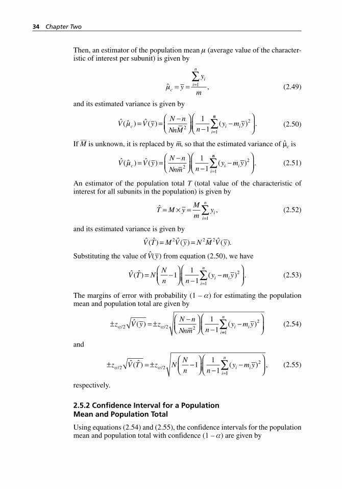
34 Chapter Two
Then, an estimator of the population mean µ (average value of the character-istic of interest per subunit) is given by
ˆ ,µc
ii
n
y
y
m= = =
∑1
(2.49)
and its estimated variance is given by
ˆ ( ˆ ) ˆ ( ) ( )V V yN n
NnM ny m yc i i
i
µ = =−⎛
⎝⎜⎞⎠⎟ −
−=
22
1
1
1
nn
∑⎛
⎝⎜⎞
⎠⎟.
(2.50)
If M—
is unknown, it is replaced by m–, so that the estimated variance of µc is
ˆ ( ˆ ) ˆ ( ) ( )V V yN n
Nnm ny m yc i i
i
µ = =−⎛
⎝⎜⎞⎠⎟ −
−=
22
1
1
1
nn
∑⎛
⎝⎜⎞
⎠⎟.
(2.51)
An estimator of the population total T (total value of the characteristic of interest for all subunits in the population) is given by
ˆ ,T M yM
myi
i
n
= × ==∑
1 (2.52)
and its estimated variance is given by
ˆ ( ˆ) ˆ ( ) ˆ ( ).V T M V y N M V y= =2 2 2
Substituting the value of V(y–) from equation (2.50), we have
ˆ ( ˆ) ( ) .V T NN
n ny m yi i
i
n
= −⎛⎝⎜
⎞⎠⎟ −
−⎛
⎝⎜⎞
⎠⎟=∑1
1
12
1
(2.53)
The margins of error with probability (1 – α) for estimating the population mean and population total are given by
± = ±−⎛
⎝⎜⎞⎠⎟ −
−z V y zN n
Nnm ny m yi i
iα α/ /
ˆ ( ) ( )2 2 221
1 ==∑
⎛
⎝⎜⎞
⎠⎟1
n
(2.54)
and
± = ± −⎛⎝⎜
⎞⎠⎟ −
−=
z V T z NN
n ny m yi i
iα α/ /
ˆ ( ˆ) ( )2 221
1
1 11
n
∑⎛
⎝⎜⎞
⎠⎟,
(2.55)
respectively.
2.5.2 Confidence Interval for a Population Mean and Population Total
Using equations (2.54) and (2.55), the confidence intervals for the population mean and population total with confidence (1 – α) are given by
H1277 ch02.indd 34H1277 ch02.indd 34 3/8/07 5:31:14 PM3/8/07 5:31:14 PM
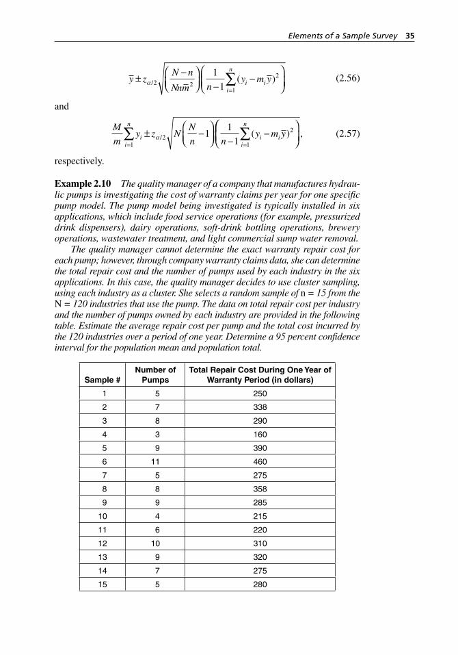
Elements of a Sample Survey 35
y zN n
Nnm ny m yi i
i
n
±−⎛
⎝⎜⎞⎠⎟ −
−⎛
⎝⎜⎞
⎠⎟=∑α/ ( )2 2
2
1
1
1
(2.56)
and
M
my z N
N
n ny m yi
i
n
i ii
n
= =∑ ∑± −
⎛⎝⎜
⎞⎠⎟ −
−1
22
1
11
1α/ ( )⎛⎛
⎝⎜⎞
⎠⎟,
(2.57)
respectively.
Example 2.10 The quality manager of a company that manufactures hydrau-lic pumps is investigating the cost of warranty claims per year for one specific pump model. The pump model being investigated is typically installed in six applications, which include food service operations (for example, pressurized drink dispensers), dairy operations, soft- drink bottling operations, brewery operations, wastewater treatment, and light commercial sump water removal.
The quality manager cannot determine the exact warranty repair cost for each pump; however, through company warranty claims data, she can determine the total repair cost and the number of pumps used by each industry in the six applications. In this case, the quality manager decides to use cluster sampling, using each industry as a cluster. She selects a random sample of n = 15 from the N = 120 industries that use the pump. The data on total repair cost per industry and the number of pumps owned by each industry are provided in the following table. Estimate the average repair cost per pump and the total cost incurred by the 120 industries over a period of one year. Determine a 95 percent confidence interval for the population mean and population total.
Sample #Number of
PumpsTotal Repair Cost During One Year of
Warranty Period (in dollars)
1 5 250
2 7 338
3 8 290
4 3 160
5 9 390
6 11 460
7 5 275
8 8 358
9 9 285
10 4 215
11 6 220
12 10 310
13 9 320
14 7 275
15 5 280
H1277 ch02.indd 35H1277 ch02.indd 35 3/8/07 5:31:14 PM3/8/07 5:31:14 PM
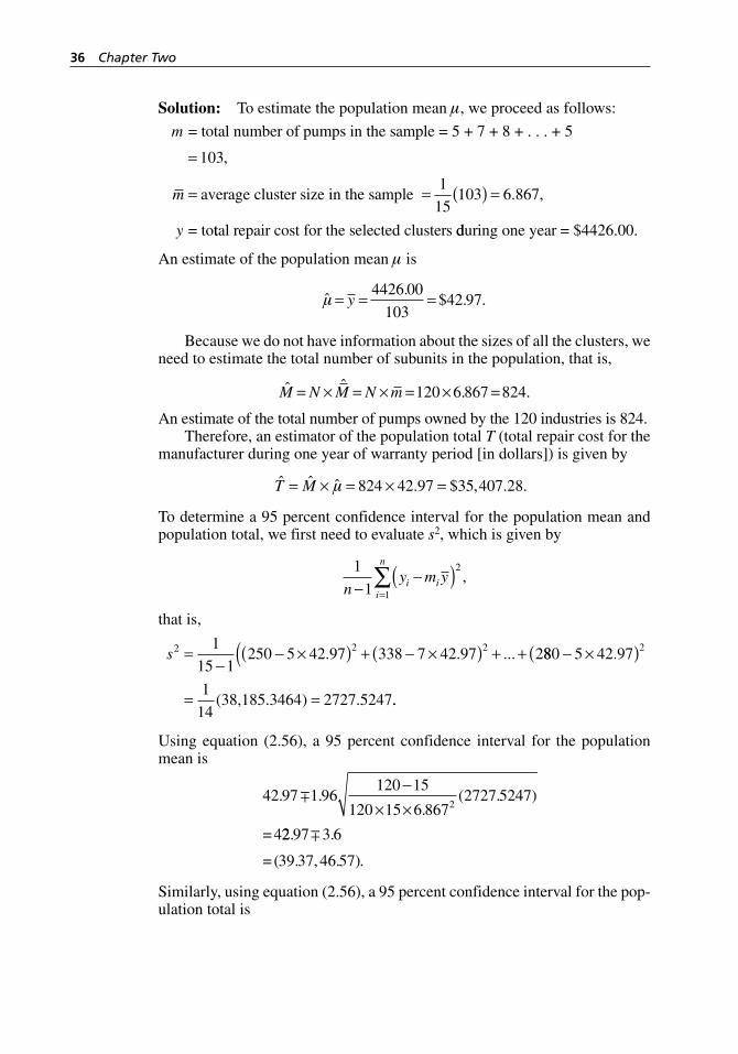
36 Chapter Two
Solution: To estimate the population mean µ, we proceed as follows:
m = total number of pumps in the sample = 5 + 7 + 8 + . . . + 5
average cluster
=
=
103,
m size in the sample
= to
= ( ) =1
15103 6 867. ,
y ttal repair cost for the selected clusters dduring one year = $4426.00.
An estimate of the population mean µ is
ˆ
.$ . .µ = = =y
4426 00
10342 97
Because we do not have information about the sizes of all the clusters, we need to estimate the total number of subunits in the population, that is,
ˆ ˆ . .M N M N m= × = × = × =120 6 867 824
An estimate of the total number of pumps owned by the 120 industries is 824.Therefore, an estimator of the population total T (total repair cost for the
manufacturer during one year of warranty period [in dollars]) is given by
ˆ ˆ ˆ . $ , . .T M= × = × =µ 824 42 97 35 407 28
To determine a 95 percent confidence interval for the population mean and population total, we first need to evaluate s2, which is given by
1
1
2
1ny m yi i
i
n
−−( )
=∑ ,
that is,
s2 2 21
15 1250 5 42 97 338 7 42 97 2=
−− ×( ) + − ×( ) + +. . ... 880 5 42 97
1
1438 185 3464 2727 5247
2− ×( )(= =
.
( , . ) . ..
Using equation (2.56), a 95 percent confidence interval for the population mean is
Similarly, using equation (2.56), a 95 percent confidence interval for the pop-ulation total is
H1277 ch02.indd 36H1277 ch02.indd 36 3/8/07 6:22:09 PM3/8/07 6:22:09 PM
Elements of a Sample Survey 37
2.5.3 Determination of Sample Size
The sample size needed to estimate the population mean with margin of error E with probability (1 – α) is given by
n
z Ns
NM E z s≥
+α
α
/
/
,22 2
2 22
2 2
(2.58)
where
s
ny m yi i
i
n2 2
1
1
1=
−−
=∑( ) .
The sample size needed to estimate the population total with margin of error E′ with probability (1 – α) can be found from equation (2.58) by replacing E with (E′/M).
Example 2.11 In Example 2.10, determine the sample size if the quality manager wants to estimate the repair cost per pump with a margin of error $2.00 with 95 percent probability.
Solution: Using equation (2.58), the desired sample size is
n ≥
+( . ) ( )( . )
( )( . ) ( )
1 96 120 2727 5247
120 6 867 2
2
2 2 (( . ) ( . ). .
1 96 2727 524737 97
2=
The sample size should be n = 38. Note that in order to determine the sample size, we needed s2 and m–, for which we need to have a sample and thus the sample size, which in fact we want to determine. The solution for this problem, as discussed in details in Applied Statistics for the Six Sigma Green Belt, is to evaluate these quantities either by using some similar data if already available or by taking a smaller sample, as we did in this example.
H1277 ch02.indd 37H1277 ch02.indd 37 3/8/07 6:22:21 PM3/8/07 6:22:21 PM

H1277 ch02.indd 38H1277 ch02.indd 38 3/8/07 5:31:15 PM3/8/07 5:31:15 PM
39
The concept of quality is centuries old. However, the concept of SQC is less than a century old. SQC is merely a set of interrelated tools that includes SPC, DOE, acceptance sampling, and other tools used
to monitor and improve quality. SPC consists of several tools that are useful for process monitoring. The quality control chart, which is the center of our discussion in this chapter, is one of these tools. Walter A. Shewhart, from Bell Telephone Laboratories, was the first person to apply statistical methods to quality improvement when, in 1924, he presented the first quality control chart. In 1931, Shewhart wrote a book on SQC titled Economic Control of Quality of Manufactured Product (D. Van Nostrand Co.). The publication of this book set the notion of SQC in full swing. In the initial stages, the accep-tance of the notion of SQC in the United States was almost negligible. It was only during World War II, when the armed services adopted the statistically designed sampling inspection schemes, that the concept of SQC started to gain acceptance in American industry.
The complete adoption of modern SQC was limited from the 1950s to the late 1970s, however, because American manufacturers believed that quality and productivity couldn’t go hand in hand. American manufacturers argued that producing goods of high quality would cost more because high qual-ity would mean buying raw materials of higher grade, hiring more qualified personnel, and providing more training to workers, all of which would trans-late into higher costs. American manufacturers also believed that producing higher- quality goods would slow down productivity because better- qualified and better- trained workers would not compromise quality to meet their daily quotas, which would further add to the cost of their product. As a consequence, they believed they would not be able to compete in the world market and would therefore lose their market share. The industrial revolution in Japan, however, proved that American manufacturers were wrong. This revolution followed the visit of a famous American statistician, W. Edwards Deming, in 1950.
Deming (1986, 2) wrote, “Improvement of quality transfers waste of man- hours and of machine- time into the manufacture of good product and better service. The result is a chain reaction—lower costs, better competitive position,
3
Phase I (Detecting Large Shifts)—SPC: Control Charts for Variables
H1277 ch03.indd 39H1277 ch03.indd 39 3/8/07 5:38:57 PM3/8/07 5:38:57 PM
40 Chapter Three
and happier people on the job, jobs and more jobs.” Deming describes this chain reaction as follows:
Improve quality → cost decreases because of less work, fewer mistakes, fewer delays or snags, better use of machine time and materials → pro-ductivity improves → capture the market with better quality and lower price → stay in business → provide jobs and more jobs. (3)
After Deming’s visit in 1950, this message of a chain reaction appeared on blackboards in every meeting room of top management in the industrial world of Japan. Once the management in Japan adopted the philosophy of this chain reaction, everyone had one common goal of achieving quality.
3.1 Basic Definition of Quality and Its Benefits
Different authors have defined the concept of quality in different ways. We define it as Deming did: a product is of good quality if it meets the needs of a customer and the customer is glad that he or she bought that product. The customer may be internal or external, an individual or a corporation. If a product meets the needs of the customer, the customer is bound to buy that product again and again. On the contrary, if a product does not meet the needs of a customer, then he or she will not buy that product even if he or she is an internal customer. Consequently, that product will be deemed of bad quality, and eventually it is bound to go out of the market.
Other components of a product’s quality are its reliability, how much maintenance it demands, and, when the need arises, how easily and how fast one can get it serviced. In evaluating the quality of a product, its attractability and rate of depreciation also play an important role.
As described by Deming in his telecast conferences, the benefits of better quality are numerous. First and foremost is that it enhances the overall image and reputation of the company by meeting the needs of its customers and thus making them happy. A happy customer is bound to buy the product again and again. Also, a happy customer is likely to share a good experience with the product with friends, relatives, and neighbors. Therefore, the company gets publicity without spending a dime, and this results in more sales and higher profits. Higher profits lead to higher stock prices, which means higher net worth of the company. Better quality provides workers satisfaction and pride in their workmanship. A satisfied worker goes home happy, which makes his or her family happy. A happy family boosts the morale of a worker, which means greater dedication and loyalty to the company.
Another benefit of better quality is decreased cost. This is due to the need for less rework, thus less scrap, fewer raw materials used, and fewer workforce hours and machine hours wasted. Ultimately, this means increased productiv-ity, a better competitive position, increased sales, and a higher market share. On the other hand, losses due to poor quality are enormous. Poor quality not only affects sales and the competitive position, but it also carries with it high hidden costs that are usually not calculated and therefore not known with precision. These costs include unusable product, product sold at a discounted
H1277 ch03.indd 40H1277 ch03.indd 40 3/8/07 5:38:58 PM3/8/07 5:38:58 PM
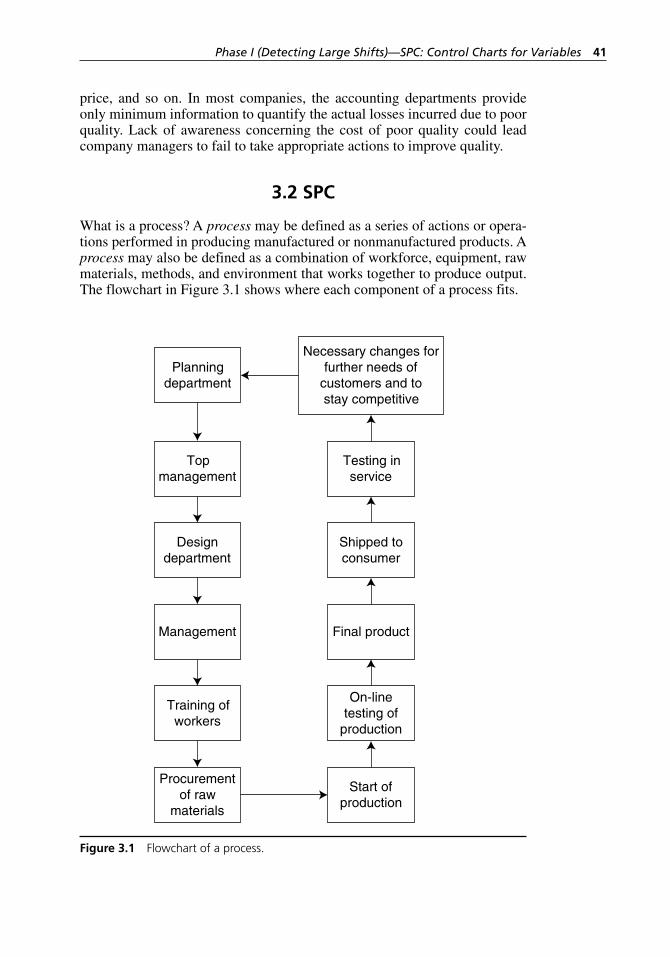
Phase I (Detecting Large Shifts)—SPC: Control Charts for Variables 41
price, and so on. In most companies, the accounting departments provide only minimum information to quantify the actual losses incurred due to poor quality. Lack of awareness concerning the cost of poor quality could lead company managers to fail to take appropriate actions to improve quality.
3.2 SPC
What is a process? A process may be defined as a series of actions or opera-tions performed in producing manufactured or nonmanufactured products. A process may also be defined as a combination of workforce, equipment, raw materials, methods, and environment that works together to produce output. The flowchart in Figure 3.1 shows where each component of a process fits.
On-linetesting of
production
Start ofproduction
Necessary changes forfurther needs of
customers and tostay competitive
Final product
Shipped toconsumer
Testing inservice
Planningdepartment
Topmanagement
Designdepartment
Management
Training ofworkers
Procurementof raw
materials
Figure 3.1 Flowchart of a process.
H1277 ch03.indd 41H1277 ch03.indd 41 3/8/07 5:38:58 PM3/8/07 5:38:58 PM
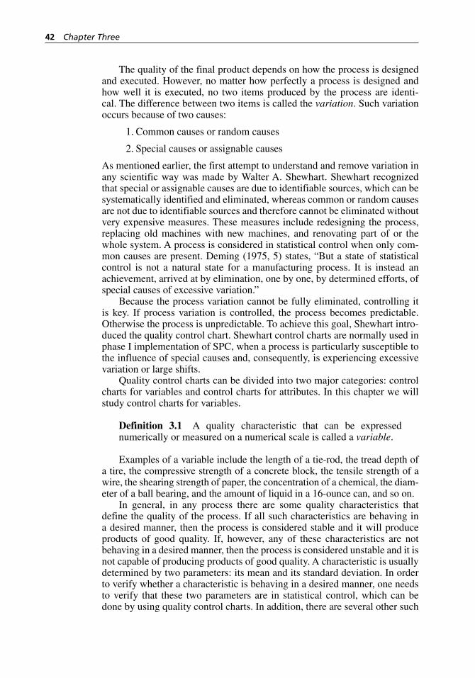
42 Chapter Three
The quality of the final product depends on how the process is designed and executed. However, no matter how perfectly a process is designed and how well it is executed, no two items produced by the process are identi-cal. The difference between two items is called the variation. Such variation occurs because of two causes:
1. Common causes or random causes
2. Special causes or assignable causes
As mentioned earlier, the first attempt to understand and remove variation in any scientific way was made by Walter A. Shewhart. Shewhart recognized that special or assignable causes are due to identifiable sources, which can be systematically identified and eliminated, whereas common or random causes are not due to identifiable sources and therefore cannot be eliminated without very expensive measures. These measures include redesigning the process, replacing old machines with new machines, and renovating part of or the whole system. A process is considered in statistical control when only com-mon causes are present. Deming (1975, 5) states, “But a state of statistical control is not a natural state for a manufacturing process. It is instead an achievement, arrived at by elimination, one by one, by determined efforts, of special causes of excessive variation.”
Because the process variation cannot be fully eliminated, controlling it is key. If process variation is controlled, the process becomes predictable. Otherwise the process is unpredictable. To achieve this goal, Shewhart intro-duced the quality control chart. Shewhart control charts are normally used in phase I implementation of SPC, when a process is particularly susceptible to the influence of special causes and, consequently, is experiencing excessive variation or large shifts.
Quality control charts can be divided into two major categories: control charts for variables and control charts for attributes. In this chapter we will study control charts for variables.
Definition 3.1 A quality characteristic that can be expressed numerically or measured on a numerical scale is called a variable.
Examples of a variable include the length of a tie- rod, the tread depth of a tire, the compressive strength of a concrete block, the tensile strength of a wire, the shearing strength of paper, the concentration of a chemical, the diam-eter of a ball bearing, and the amount of liquid in a 16-ounce can, and so on.
In general, in any process there are some quality characteristics that define the quality of the process. If all such characteristics are behaving in a desired manner, then the process is considered stable and it will produce products of good quality. If, however, any of these characteristics are not behaving in a desired manner, then the process is considered unstable and it is not capable of producing products of good quality. A characteristic is usually determined by two parameters: its mean and its standard deviation. In order to verify whether a characteristic is behaving in a desired manner, one needs to verify that these two parameters are in statistical control, which can be done by using quality control charts. In addition, there are several other such
H1277 ch03.indd 42H1277 ch03.indd 42 3/8/07 5:38:58 PM3/8/07 5:38:58 PM
Phase I (Detecting Large Shifts)—SPC: Control Charts for Variables 43
tools that are valuable in achieving process stability. These tools, including the control charts, constitute an integral part of SPC. SPC is very useful in any process related to manufacturing, service, or retail industries. This set of tools consists of the following:
1. Histogram
2. Stem-and-leaf diagram
3. Scatter diagram
4. Run chart (also known as a line graph or a time series graph)
5. Check sheet
6. Pareto chart
7. Cause-and-effect diagram (also known as a fishbone or Ishikawa diagram)
8. Defect concentration diagram
9. Control charts
These tools of SPC form a simple but very powerful structure for quality improvement. Once workers become fully familiar with these tools, manage-ment must get involved to implement SPC for an ongoing quality- improvement process. Management must create an environment where these tools become part of the day- to-day production or service process. The implementation of SPC without management’s involvement and cooperation is bound to fail. In addition to discussing these tools, we will also explore here some of the ques-tions that arise while implementing SPC.
Every job, whether in a manufacturing company or in a service company, involves a process. As described earlier, each process consists of a certain number of steps. No matter how well the process is planned, designed, and executed, there is always some potential for variability. In some cases this variability may be very little, while in other cases it may be very high. If the variability is very little, it is usually due to some common causes that are unavoidable and cannot be controlled. If the variability is too high, we expect that in addition to the common causes there are some other causes, usually known as assignable causes, present in the process. Any process working under only common causes or chance causes is considered to be in statistical control. If a process is working under both common and assignable causes, it is considered unstable, or not in statistical control.
The first four tools in the SPC tools list are discussed in the first volume of this series, Applied Statistics for the Six Sigma Green Belt. In this chapter and the two that follow, we will discuss the rest of these tools.
Check Sheet
In order to improve the quality of a product, management must try to reduce the variation of all the quality characteristics; that is, the process must be brought to a stable condition. In any SPC procedure used to stabilize a process, it is
H1277 ch03.indd 43H1277 ch03.indd 43 3/8/07 5:38:58 PM3/8/07 5:38:58 PM
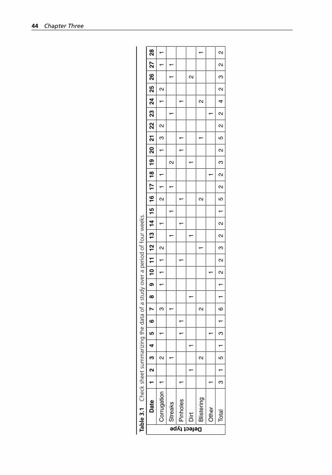
44 Chapter Three
Tab
le 3
.1
Che
ck s
heet
sum
mar
izin
g th
e da
ta o
f a
stud
y ov
er a
per
iod
of f
our
wee
ks.
Defect type
Dat
e1
23
45
67
89
1011
1213
1415
1617
1819
2021
2223
2425
2627
28
Cor
ruga
tion
12
13
11
12
12
11
13
21
21
1
Str
eaks
11
11
12
11
1
Pin
hole
s1
11
11
11
11
Dir
t1
11
11
2
Blis
terin
g2
21
21
21
Oth
er1
11
11
Tota
l3
15
13
16
11
22
32
21
52
23
25
22
42
32
2
H1277 ch03.indd 44H1277 ch03.indd 44 3/8/07 5:38:58 PM3/8/07 5:38:58 PM
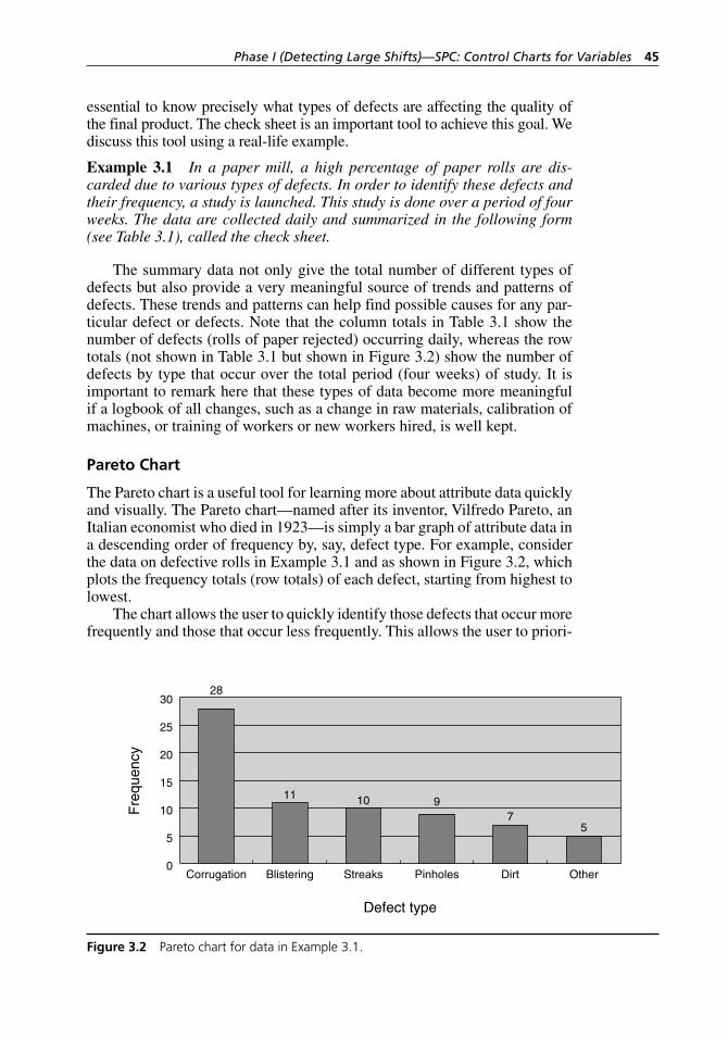
Phase I (Detecting Large Shifts)—SPC: Control Charts for Variables 45
essential to know precisely what types of defects are affecting the quality of the final product. The check sheet is an important tool to achieve this goal. We discuss this tool using a real- life example.
Example 3.1 In a paper mill, a high percentage of paper rolls are dis-carded due to various types of defects. In order to identify these defects and their frequency, a study is launched. This study is done over a period of four weeks. The data are collected daily and summarized in the following form (see Table 3.1), called the check sheet.
The summary data not only give the total number of different types of defects but also provide a very meaningful source of trends and patterns of defects. These trends and patterns can help find possible causes for any par-ticular defect or defects. Note that the column totals in Table 3.1 show the number of defects (rolls of paper rejected) occurring daily, whereas the row totals (not shown in Table 3.1 but shown in Figure 3.2) show the number of defects by type that occur over the total period (four weeks) of study. It is important to remark here that these types of data become more meaningful if a logbook of all changes, such as a change in raw materials, calibration of machines, or training of workers or new workers hired, is well kept.
Pareto Chart
The Pareto chart is a useful tool for learning more about attribute data quickly and visually. The Pareto chart—named after its inventor, Vilfredo Pareto, an Italian economist who died in 1923—is simply a bar graph of attribute data in a descending order of frequency by, say, defect type. For example, consider the data on defective rolls in Example 3.1 and as shown in Figure 3.2, which plots the frequency totals (row totals) of each defect, starting from highest to lowest.
The chart allows the user to quickly identify those defects that occur more frequently and those that occur less frequently. This allows the user to priori-
0
5
10
15
20
25
30
OtherDirtPinholesStreaksBlisteringCorrugation
28
11 10 97
5
Defect type
Fre
quen
cy
Figure 3.2 Pareto chart for data in Example 3.1.
H1277 ch03.indd 45H1277 ch03.indd 45 3/8/07 5:38:59 PM3/8/07 5:38:59 PM
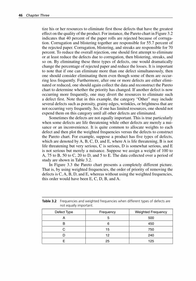
46 Chapter Three
tize his or her resources to eliminate first those defects that have the greatest effect on the quality of the product. For instance, the Pareto chart in Figure 3.2 indicates that 40 percent of the paper rolls are rejected because of corruga-tion. Corrugation and blistering together are responsible for 55.7 percent of the rejected paper. Corrugation, blistering, and streaks are responsible for 70 percent. To reduce the overall rejection, one should first attempt to eliminate or at least reduce the defects due to corrugation, then blistering, streaks, and so on. By eliminating these three types of defects, one would dramatically change the percentage of rejected paper and reduce the losses. It is important to note that if one can eliminate more than one defect simultaneously, then one should consider eliminating them even though some of them are occur-ring less frequently. Furthermore, after one or more defects are either elimi-nated or reduced, one should again collect the data and reconstruct the Pareto chart to determine whether the priority has changed. If another defect is now occurring more frequently, one may divert the resources to eliminate such a defect first. Note that in this example, the category “Other” may include several defects such as porosity, grainy edges, wrinkles, or brightness that are not occurring very frequently. So, if one has limited resources, one should not expend them on this category until all other defects are eliminated.
Sometimes the defects are not equally important. This is true particularly when some defects are life threatening while other defects are merely a nui-sance or an inconvenience. It is quite common to allocate weights to each defect and then plot the weighted frequencies versus the defects to construct the Pareto chart. For example, suppose a product has five types of defects, which are denoted by A, B, C, D, and E, where A is life threatening, B is not life threatening but very serious, C is serious, D is somewhat serious, and E is not serious but merely a nuisance. Suppose we assign a weight of 100 to A, 75 to B, 50 to C, 20 to D, and 5 to E. The data collected over a period of study are shown in Table 3.2.
In Figure 3.3 the Pareto chart presents a completely different picture. That is, by using weighted frequencies, the order of priority of removing the defects is C, A, B, D, and E, whereas without using the weighted frequencies, this order would have been E, C, D, B, and A.
Table 3.2 Frequencies and weighted frequencies when different types of defects are not equally important.
Defect Type Frequency Weighted Frequency
A 5 500
B 6 450
C 15 750
D 12 240
E 25 125
H1277 ch03.indd 46H1277 ch03.indd 46 3/8/07 5:38:59 PM3/8/07 5:38:59 PM
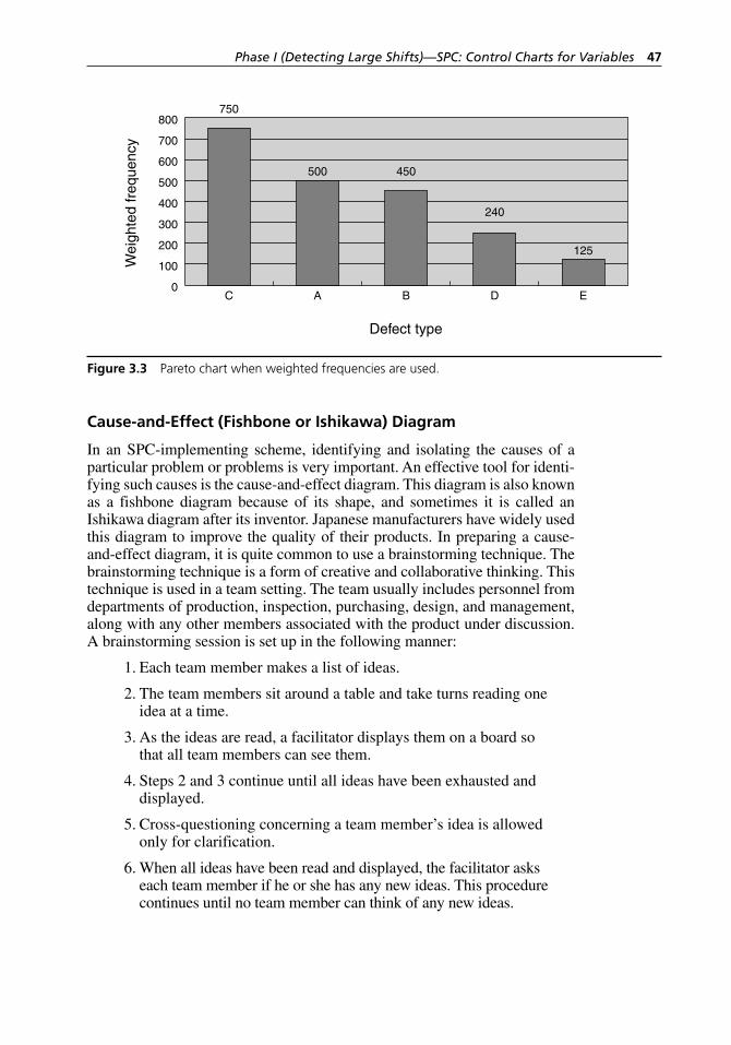
Phase I (Detecting Large Shifts)—SPC: Control Charts for Variables 47
Cause-and-Effect (Fishbone or Ishikawa) Diagram
In an SPC- implementing scheme, identifying and isolating the causes of a particular problem or problems is very important. An effective tool for identi-fying such causes is the cause- and-effect diagram. This diagram is also known as a fishbone diagram because of its shape, and sometimes it is called an Ishikawa diagram after its inventor. Japanese manufacturers have widely used this diagram to improve the quality of their products. In preparing a cause- and-effect diagram, it is quite common to use a brainstorming technique. The brainstorming technique is a form of creative and collaborative thinking. This technique is used in a team setting. The team usually includes personnel from departments of production, inspection, purchasing, design, and management, along with any other members associated with the product under discussion. A brainstorming session is set up in the following manner:
1. Each team member makes a list of ideas.
2. The team members sit around a table and take turns reading one idea at a time.
3. As the ideas are read, a facilitator displays them on a board so that all team members can see them.
4. Steps 2 and 3 continue until all ideas have been exhausted and displayed.
5. Cross-questioning concerning a team member’s idea is allowed only for clarification.
6. When all ideas have been read and displayed, the facilitator asks each team member if he or she has any new ideas. This procedure continues until no team member can think of any new ideas.
0
100
200
300
400
500
600
700
800750
500 450
240
125
EDBAC
Wei
ghte
d fr
eque
ncy
Defect type
Figure 3.3 Pareto chart when weighted frequencies are used.
H1277 ch03.indd 47H1277 ch03.indd 47 3/8/07 5:38:59 PM3/8/07 5:38:59 PM
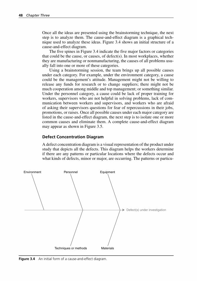
48 Chapter Three
Once all the ideas are presented using the brainstorming technique, the next step is to analyze them. The cause- and-effect diagram is a graphical tech-nique used to analyze these ideas. Figure 3.4 shows an initial structure of a cause- and-effect diagram.
The five spines in Figure 3.4 indicate the five major factors or categories that could be the cause, or causes, of defect(s). In most workplaces, whether they are manufacturing or nonmanufacturing, the causes of all problems usu-ally fall into one or more of these categories.
Using a brainstorming session, the team brings up all possible causes under each category. For example, under the environment category, a cause could be the management’s attitude. Management might not be willing to release any funds for research or to change suppliers; there might not be much cooperation among middle and top management; or something similar. Under the personnel category, a cause could be lack of proper training for workers, supervisors who are not helpful in solving problems, lack of com-munication between workers and supervisors, and workers who are afraid of asking their supervisors questions for fear of repercussions in their jobs, promotions, or raises. Once all possible causes under each major category are listed in the cause- and-effect diagram, the next step is to isolate one or more common causes and eliminate them. A complete cause- and-effect diagram may appear as shown in Figure 3.5.
Defect Concentration Diagram
A defect concentration diagram is a visual representation of the product under study that depicts all the defects. This diagram helps the workers determine if there are any patterns or particular locations where the defects occur and what kinds of defects, minor or major, are occurring. The patterns or particu-
Environment Personnel Equipment
Techniques or methods Materials
Defect(s) under investigation
Figure 3.4 An initial form of a cause- and-effect diagram.
H1277 ch03.indd 48H1277 ch03.indd 48 3/8/07 5:38:59 PM3/8/07 5:38:59 PM
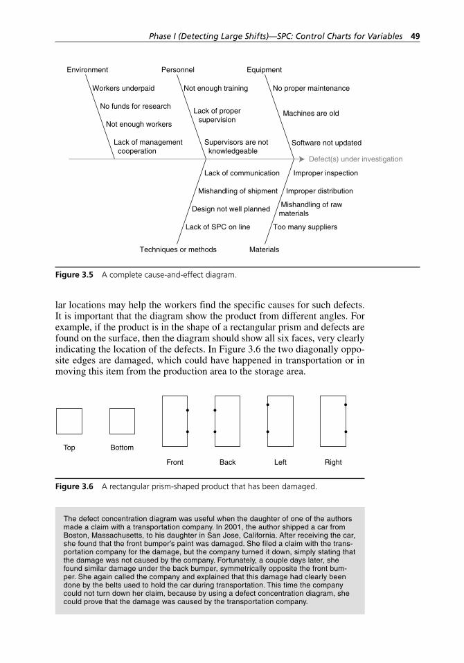
Phase I (Detecting Large Shifts)—SPC: Control Charts for Variables 49
lar locations may help the workers find the specific causes for such defects. It is important that the diagram show the product from different angles. For example, if the product is in the shape of a rectangular prism and defects are found on the surface, then the diagram should show all six faces, very clearly indicating the location of the defects. In Figure 3.6 the two diagonally oppo-site edges are damaged, which could have happened in transportation or in moving this item from the production area to the storage area.
Environment Personnel Equipment
Techniques or methods Materials
Defect(s) under investigation
Workers underpaid Not enough training No proper maintenance
No funds for research
Not enough workers
Lack of propersupervision
Machines are old
Lack of management cooperation
Lack of communication Improper inspection
Mishandling of shipment Improper distribution
Design not well planned Mishandling of rawmaterials
Lack of SPC on line Too many suppliers
Supervisors are not knowledgeable
Software not updated
Figure 3.5 A complete cause- and-effect diagram.
Top Bottom
Front Back Left Right
Figure 3.6 A rectangular prism- shaped product that has been damaged.
The defect concentration diagram was useful when the daughter of one of the authors made a claim with a transportation company. In 2001, the author shipped a car from Boston, Massachusetts, to his daughter in San Jose, California. After receiving the car, she found that the front bumper’s paint was damaged. She filed a claim with the trans-portation company for the damage, but the company turned it down, simply stating that the damage was not caused by the company. Fortunately, a couple days later, she found similar damage under the back bumper, symmetrically opposite the front bum-per. She again called the company and explained that this damage had clearly been done by the belts used to hold the car during transportation. This time the company could not turn down her claim, because by using a defect concentration diagram, she could prove that the damage was caused by the transportation company.
H1277 ch03.indd 49H1277 ch03.indd 49 3/8/07 5:38:59 PM3/8/07 5:38:59 PM
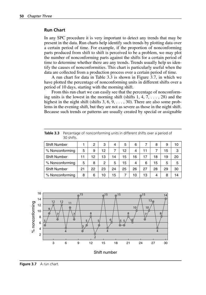
50 Chapter Three
Run Chart
In any SPC procedure it is very important to detect any trends that may be present in the data. Run charts help identify such trends by plotting data over a certain period of time. For example, if the proportion of nonconforming parts produced from shift to shift is perceived to be a problem, we may plot the number of nonconforming parts against the shifts for a certain period of time to determine whether there are any trends. Trends usually help us iden-tify the causes of nonconformities. This chart is particularly useful when the data are collected from a production process over a certain period of time.
A run chart for data in Table 3.3 is shown in Figure 3.7, in which we have plotted the percentage of nonconforming units in different shifts over a period of 10 days, starting with the morning shift.
From this run chart we can easily see that the percentage of nonconform-ing units is the lowest in the morning shift (shifts 1, 4, 7, . . . , 28) and the highest in the night shift (shifts 3, 6, 9, . . . , 30). There are also some prob-lems in the evening shift, but they are not as severe as those in the night shift. Because such trends or patterns are usually created by special or assignable
Table 3.3 Percentage of nonconforming units in different shifts over a period of 30 shifts.
Shift Number 1 2 3 4 5 6 7 8 9 10
% Nonconforming 5 9 12 7 12 4 11 7 15 3
Shift Number 11 12 13 14 15 16 17 18 19 20
% Nonconforming 5 8 2 5 15 4 6 15 5 5
Shift Number 21 22 23 24 25 26 27 28 29 30
% Nonconforming 8 6 10 15 7 10 13 4 8 14
2
4
6
8
10
12
14
16
30272421181512963
% n
onco
nfor
min
g
Shift number
5
9
12 12
4
11
7 7 7
15
3
5
8 8 8
2
5 5 5
15 15 15
4 4
6 6
10 10
13
14
Figure 3.7 A run chart.
H1277 ch03.indd 50H1277 ch03.indd 50 3/8/07 5:38:59 PM3/8/07 5:38:59 PM
Phase I (Detecting Large Shifts)—SPC: Control Charts for Variables 51
causes, the run chart will certainly prompt the management to explore how the various shifts differ. Does the quality of the raw materials differ from shift to shift? Is there inadequate training of workers in the later shifts? Are evening- and late- shift workers more susceptible to fatigue? Are there envi-ronmental problems that increase in severity as the day wears on?
Deming (1986, 313) points out that sometimes the frequency distribution of a set of data does not give a true picture of the data, whereas a run chart can bring out the real problems of the data. The frequency distribution gives us the overall picture of the data, but it does not show us any trends or patterns that may be present in the process on a short- term basis.
Control charts make up perhaps the most important part of SPC. We will study some of the basic concepts of control charts in the following section, and then in the rest of this chapter and the next two chapters we will study the various kinds of control charts.
3.3 Control Charts for Variables
A control chart is a simple but very powerful statistical device used to keep a process predictable. As noted by Duncan (1986), a control chart is (1) a device for describing in concrete terms what a state of statistical control is, (2) a device for attaining control, and (3) a device for judging whether control has been attained.
Before the control charts are implemented in any process, it is important to understand the process and have a concrete plan for future actions that would be needed to improve the process.
Process Evaluation
Process evaluation includes not only the study of the final product, but also the study of all the intermediate steps or outputs that describes the actual operating state of the process. For example, in the paper production process, wood chips and pulp may be considered as intermediate outputs. If the data on process evaluation are collected, analyzed, and interpreted correctly, they can show where and when a corrective action is necessary to make the whole process work more efficiently.
Action on Process
Action on process is important for any process because it prevents the pro-duction of an out- of-specification product. An action on process may include changes in raw materials, operator training, equipment, design, or other mea-sures. The effects of such actions on a process should be monitored closely, and further action should be taken if necessary.
Action on Output
If the process evaluation indicates that no further action on the process is necessary, the last action is to ship the final product to its destination. Note
H1277 ch03.indd 51H1277 ch03.indd 51 3/8/07 5:39:00 PM3/8/07 5:39:00 PM
52 Chapter Three
that some people believe action on output consists of sampling plans and dis-carding the out- of-specification product, which has already been produced. Obviously, such an action on the output is futile and expensive. We are inter-ested in correcting the output before it is produced. This goal can be achieved through the use of control charts.
Any process with a lot of variation is bad and is bound to produce prod-ucts of inferior quality. Control charts can help detect variation in any pro-cess. As described earlier, in any process there are two causes of variation: common causes or random causes, and special causes or assignable causes.
Variation
No process can produce two products that are exactly alike or possess exactly the same characteristics. Any process is bound to contain some sources of variation. The difference between two products may be very large, moderate, very small, or even undetectable, depending on the source of variation, but certainly there is always some difference. For example, the moisture content in any two rolls of paper, the opacity in any two spools of paper, and the brightness of two lots of pulp will always vary. Our aim is to trace back as far as possible the sources of such variation and eliminate them. The first step is to separate the common and special causes of such sources of variation.
Common Causes or Random Causes
Common causes or random causes are the sources of variation within a pro-cess that is in statistical control. The causes behave like a constant system of chance. While individual measured values may all be different, as a group they tend to form a pattern that can be explained by a statistical distribution that can generally be characterized by:
1. Location parameter
2. Dispersion parameter
3. Shape (the pattern of variation, whether it is symmetrical, right skewed, left skewed, and so on)
Special Causes or Assignable Causes
Special causes or assignable causes refer to any source of variation that can-not be adequately explained by any single distribution of the process out-put, as otherwise would be the case if the process were in statistical control. Unless all the special causes of variation are identified and corrected, they will continue to affect the process output in an unpredictable way. Any pro-cess with assignable causes is considered unstable and hence not in statistical control. However, any process free of assignable causes is considered stable and therefore in statistical control. Assignable causes can be corrected by local actions, while common causes or random causes can be corrected only by actions on the system.
H1277 ch03.indd 52H1277 ch03.indd 52 3/8/07 5:39:00 PM3/8/07 5:39:00 PM
Phase I (Detecting Large Shifts)—SPC: Control Charts for Variables 53
Local Actions and Actions on the System
Local Actions
1. Are usually required to eliminate special causes of variation
2. Can usually be taken by people close to the process
3. Can correct about 15 percent of process problems
Deming (1982) believed that as much as 6 percent of all system variations is due to special or assignable causes, while no more than 94 percent of the variations is due to common causes.
Actions on the System
1. Are usually required to reduce the variation due to common causes
2. Almost always require management action for correction
3. Are needed to correct about 85 percent of process problems
Furthermore, Deming (1951) points out that there is an important relation-ship between the two types of variations and the two types of actions needed to reduce such variations. We will discuss this point in more detail.
Special causes of variation can be detected by simple statistical tech-niques. These causes of variation are not the same in all the operations involved. Detecting special causes of variation and removing them is usually the responsibility of someone directly connected to the operation, although management is sometimes in a better position to correct them. Resolving a special cause of variation usually requires local action.
The extent of common causes of variation can be indicated by simple statistical techniques, but the causes themselves need more exploration in order to be isolated. It is usually management’s responsibility to correct the common causes of variation, although personnel directly involved with the operation are sometimes in a better position to identify such causes and pass them on to management for an appropriate action. Overall, resolving com-mon causes of variation usually requires action on the system.
As we noted earlier, about 15 percent (or according to Deming, 6 per-cent) of industrial process troubles are correctable by the local action taken by people directly involved with the operation, while 85 percent are correct-able only by management’s action on the system. Confusion about the type of action required is very costly to the organization in terms of wasted efforts, delayed resolution of trouble, and other aggravating problems. So, it would be wrong to take local action (for example, changing an operator or calibrat-ing a machine) when, in fact, management action on the system was required (for example, selecting a supplier that can provide better and consistent raw materials).
All of this reasoning shows that strong statistical analysis of any opera-tion in any industrial production is necessary. Control charts are perhaps the best tool to separate the special causes from the common causes.
H1277 ch03.indd 53H1277 ch03.indd 53 3/8/07 5:39:00 PM3/8/07 5:39:00 PM
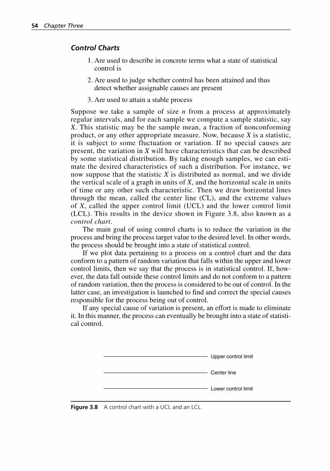
54 Chapter Three
Control Charts
1. Are used to describe in concrete terms what a state of statistical control is
2. Are used to judge whether control has been attained and thus detect whether assignable causes are present
3. Are used to attain a stable process
Suppose we take a sample of size n from a process at approximately regular intervals, and for each sample we compute a sample statistic, say X. This statistic may be the sample mean, a fraction of nonconforming product, or any other appropriate measure. Now, because X is a statistic, it is subject to some fluctuation or variation. If no special causes are present, the variation in X will have characteristics that can be described by some statistical distribution. By taking enough samples, we can esti-mate the desired characteristics of such a distribution. For instance, we now suppose that the statistic X is distributed as normal, and we divide the vertical scale of a graph in units of X, and the horizontal scale in units of time or any other such characteristic. Then we draw horizontal lines through the mean, called the center line (CL), and the extreme values of X, called the upper control limit (UCL) and the lower control limit (LCL). This results in the device shown in Figure 3.8, also known as a control chart.
The main goal of using control charts is to reduce the variation in the process and bring the process target value to the desired level. In other words, the process should be brought into a state of statistical control.
If we plot data pertaining to a process on a control chart and the data conform to a pattern of random variation that falls within the upper and lower control limits, then we say that the process is in statistical control. If, how-ever, the data fall outside these control limits and do not conform to a pattern of random variation, then the process is considered to be out of control. In the latter case, an investigation is launched to find and correct the special causes responsible for the process being out of control.
If any special cause of variation is present, an effort is made to eliminate it. In this manner, the process can eventually be brought into a state of statisti-cal control.
Center line
Upper control limit
Lower control limit
Figure 3.8 A control chart with a UCL and an LCL.
H1277 ch03.indd 54H1277 ch03.indd 54 3/8/07 5:39:00 PM3/8/07 5:39:00 PM
Phase I (Detecting Large Shifts)—SPC: Control Charts for Variables 55
Shewhart strongly recommended that a process should not be judged to be in control unless the pattern of random variation has persisted for some time and for a sizable volume of output.
Note: If a control chart shows a process in statistical control, it does not mean that all special causes have been completely eliminated; rather, it sim-ply means that for all practical purposes, it is reasonable to assume or adopt a hypothesis of common causes only.
Preparation for Use of Control Charts
In order for control charts to serve their intended purpose, it is important to take the following preparatory steps prior to implementing the control charts:
1. Establish an environment suitable for action: Any statistical method will fail unless management has prepared a responsive environment.
2. Define the process and determine the characteristics to be studied: The process must be understood in terms of its relationship to the other operations and users and in terms of the process elements (for example, people, equipment, materials, methods, and environment) that affect it at each stage. Some of the techniques discussed earlier, such as the Pareto chart or the fishbone diagram, can help make these relationships visible. Once the process is well understood, the next step is to determine which characteristics are affecting the process, which characteristics should be studied in depth, and which characteristics should be controlled.
3. Determine the correlation between characteristics: For an efficient and effective study, take advantage of the relationship between characteristics. If several characteristics of an item are positively correlated, it may be sufficient to chart only one of them. If there are some characteristics that are negatively correlated, a deeper study is required before any corrective action on such characteristics can be taken.
4. Define the measurement system: The characteristic must be operationally defined so that the findings can be communicated to all concerned in ways that have the same meaning today as they did yesterday. This includes specifying what information is to be gathered, where it should be gathered, how it should be gathered, and under what conditions it should be gathered. The operational definition is very important for collecting data because it can impact the control charts in many ways. Moreover, the analysis of data depends on how the data are collected. This is why it is extremely important that the data contain the pertinent information and are valid (for example, appropriate sampling
H1277 ch03.indd 55H1277 ch03.indd 55 3/8/07 5:39:00 PM3/8/07 5:39:00 PM
56 Chapter Three
schemes are used) so that the analysis and the interpretation of the results are done appropriately. Moreover, one should always keep in mind that each measurement system has its own inherent variability. Thus, the accuracy of any measurement system is as important as the elimination of the special causes affecting the process.
5. Minimize unnecessary variation: Unnecessary external causes of variation should be reduced before the study begins. Methods for reducing these causes include overcontrolling the process and avoiding obvious problems that could and should be corrected even without the use of control charts. Note that in all cases a process log should be kept. It should include all relevant events (big or small) such as procedural changes, new raw materials, or change of operators. This will aid in the analysis of subsequent problems.
6. Consider the customer’s needs: This includes any subsequent processes that use the product or service as an input and the final end- item customer. For example, a computer manufacturing company is a customer of the semiconductor industry; a car manufacturing company is a customer of tire manufacturing companies; and in a paper mill, the papermaking unit is a customer of the pulp- making unit.
Note that the most important quality characteristic is to produce what the cus-tomer wants. In other words, the company should deliver a product that meets the needs of the customer. A company may produce excellent things, but if it can’t meet the needs of the customer, then the customer is not going to buy that product. So, for example, the pulp- making mill should produce the kind of pulp wanted by the papermaking mill. In this particular case, the pulp and paper mills are part of the same company, but if the pulp- making mill cannot deliver the kind of pulp the papermaking mill needs, the papermaking mill will seek another supplier. Process innovation and customer satisfaction are the most important factors in the success of any manufacturing process.
Benefits of Control Charts
Properly used control charts can:
1. Be used by operators for ongoing control of a process
2. Help the process perform consistently and predictably
3. Allow the process to achieve higher quality, higher effective capacity (because there will be either no rejection or less rejection), and hence a lower cost per unit
4. Provide a common language for discussing process performance
5. Help distinguish special causes from common causes for variability and serve as a guide for management to take local action or action on the system
H1277 ch03.indd 56H1277 ch03.indd 56 3/8/07 5:39:00 PM3/8/07 5:39:00 PM
Phase I (Detecting Large Shifts)—SPC: Control Charts for Variables 57
Rational Samples for a Control Chart
It is important to note that the samples used to prepare a control chart should represent subgroups of output that are as homogeneous as possible. In other words, the subgroups should be such that if special causes are present, they will show up in differences between the subgroups rather than in differences between the members of a subgroup. A natural subgroup, for example, would be the output of a given shift. It is not correct to take the product of an arbi-trary period of time as a subgroup, especially if the subgroup overlapped two or more shifts. This is because if a sample comes from two or more shifts, any differences between the shifts will be averaged out, and consequently, the plotted point won’t indicate the presence of any special causes due to shifts. As another example, if the process used six machines, it would be bet-ter to take a sample from the output of each machine than to have a sample that consists of items from all six machines. This is because the difference between the machines may be the special cause of variation. It will be easier to detect this special cause if a sample is taken from each machine. Thus, it is true that careful selection of a subgroup or sample is perhaps the most important item in setting up a control chart.
The next step in selecting a sample is to determine the sample size. Fac-tors usually considered in determining the sample size and the frequency of the samples are the average run length (ARL) and the operating characteristic curve, also known as an OC curve. We will discuss both the ARL and the OC curve.
ARL
Definition 3.2 A run is a number of successive points plotted in a control chart.
Definition 3.3 An average run length is the average number of points plotted before a point falls outside the control limits, indicat-ing the process is out of control.
In Shewhart control charts, the ARL can be determined by using the formula
ARL =
1
p,
(3.1)
where p is the probability that any point will fall outside the control limits. It is quite common to use ARL as a benchmark for checking the performance of a control chart.
To illustrate, consider a process quality characteristic that is normally distributed. For an X
– control chart with 3σ control limits, the probability that
a point will fall outside the control limits when the process is stable is p = 0.0027, which is the probability that a normal random variable deviates from the mean µ by at least 3σ. The ARL for the X
– control chart when the process
is stable is
H1277 ch03.indd 57H1277 ch03.indd 57 3/8/07 5:39:01 PM3/8/07 5:39:01 PM
58 Chapter Three
ARL0
1
0 0027370= =
..
In other words, when the process is stable, we should expect that, on the average, an out- of-control signal or false alarm will occur once in every 370 samples. The ARL can also be used to determine how often a false alarm will occur, simply by multiplying the ARL0 by the time t between the samples. For example, if samples are taken every 30 minutes, a false alarm will occur on the average once every 185 hours. On the other hand, ARL can be used in the same manner to find out how long it will take before a given shift in the process mean is detected. This concept, which we are going to discuss in depth in section 3.3, is illustrated in the following example using an X
– control
chart.
Example 3.2 Suppose a process quality characteristic that is normally distributed is plotted in a Shewhart X
– control chart with 3σ control limits.
Suppose that the process mean µ0 experiences an upward shift of 1.5σ. Deter-mine how long, on the average, it will take to detect this shift if a sample of size four is taken every hour.
Solution: Because the process mean has experienced an upward shift of 1.5σ, the new process mean will be µ0 + 1.5σ. Furthermore, because the sam-ple size is four, the UCL in this case is also µ σ µ
σµ σ0 0 03 3
41 5+ = + = +x . .
In other words, the CL of the control chart will coincide with the UCL. The probability p that a point will fall beyond the control limits is
p P z P z= ≤ − + ≥
≅ +
=
( ) ( )
. .
. .
6 0
0 00000 0 5
0 5
Consequently, the ARL is given by
ARL = =
1
0 52
..
Therefore, it will take an average of two hours to detect a shift of 1.5σ in the process mean.
In practice, the decision of how large the samples should be and how frequently they should be taken is based on the cost of taking samples and how quickly one would like to detect the shift. Large samples taken more frequently would certainly give better protection against shifts because it will take less time to detect any given shift. For instance, in Example 3.2, if the samples are taken every half hour instead of every hour, then it will take only one hour instead of two to detect the shift of 1.5σ, and the process will produce fewer nonconforming units. So, when calculating the cost of taking samples, one must consider how much money will be saved by detecting the shift more quickly and producing fewer nonconforming units.
H1277 ch03.indd 58H1277 ch03.indd 58 3/8/07 5:39:01 PM3/8/07 5:39:01 PM
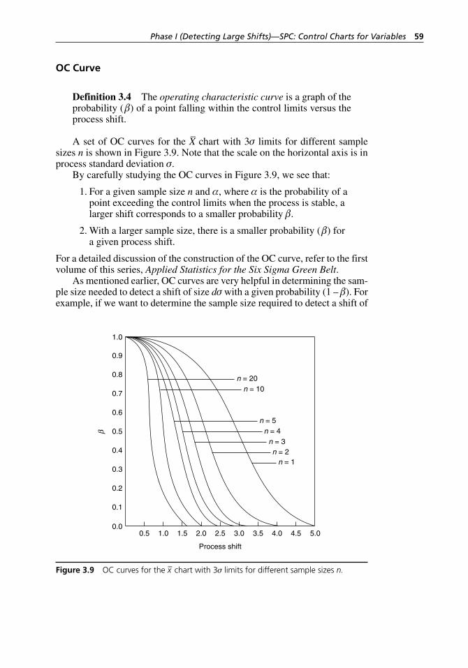
Phase I (Detecting Large Shifts)—SPC: Control Charts for Variables 59
OC Curve
Definition 3.4 The operating characteristic curve is a graph of the probability ( β) of a point falling within the control limits versus the process shift.
A set of OC curves for the X– chart with 3σ limits for different sample sizes n is shown in Figure 3.9. Note that the scale on the horizontal axis is in process standard deviation σ.
By carefully studying the OC curves in Figure 3.9, we see that:
1. For a given sample size n and α, where α is the probability of a point exceeding the control limits when the process is stable, a larger shift corresponds to a smaller probability β.
2. With a larger sample size, there is a smaller probability ( β) for a given process shift.
For a detailed discussion of the construction of the OC curve, refer to the first volume of this series, Applied Statistics for the Six Sigma Green Belt.
As mentioned earlier, OC curves are very helpful in determining the sam-ple size needed to detect a shift of size dσ with a given probability (1 – β). For example, if we want to determine the sample size required to detect a shift of
0.0
0.1
0.2
0.3
0.4
0.5
0.6
0.7
0.8
0.9
1.0
5.04.54.03.53.02.52.01.51.00.5
n = 20n = 10
n = 1n = 2
n = 5n = 4
n = 3
Process shift
Figure 3.9 OC curves for the x– chart with 3σ limits for different sample sizes n.
H1277 ch03.indd 59H1277 ch03.indd 59 3/8/07 5:39:01 PM3/8/07 5:39:01 PM
60 Chapter Three
1σ with probability 95 percent, from Figure 3.9, with d = 1 and β = 0.05, we find the size n will be slightly higher than 20.
Having studied some basic concepts of control charts, we now discuss some special control charts that are very popular and useful in any industry, manufacturing or nonmanufacturing.
3.3.1 Shewhart X– and R Control Charts
Certain rules are widely followed in preparing Shewhart X– and R control charts:
1. Take a series of samples from the process under investigation. Samples consisting of four or five items taken frequently are usually good, for the following reasons:
a. Samples of size four or five are more cost effective.
b. If samples are larger than 10, the estimate of process standard deviation obtained using the range is not very efficient. Moreover, the R chart is also not very effective.
c. With samples of size four or five, there are fewer chances for any special causes occurring during the collection of a sample. It is commonly known that if the type of variation is changing (special cause vs. common cause variation), the sample size should be as small as possible so that the average of samples does not mask the changes.
2. Enough samples should be collected so that the major source of variation has an opportunity to occur. Generally, at least 25 samples of size four or five is considered sufficient to give a good test for process stability.
3. During the collection of data, a complete log of any changes in the process, such as changes in raw materials, operators, or tools or any calibration of tools, machines, and so on, must be maintained. Keeping a log is important for finding the special causes in a process.
Calculation of Sample Statistics
The sample statistics that need to be determined in order to prepare Shewhart X– and R control charts are the sample mean (x–) and the sample range (R). For
example, let x1, x2, . . . , xn be a random sample from a process that is under investigation. We have
x
x x x
nn=
+ + +1 2 ...,
(3.2)
R x xi i= −max min( ) ( ).
(3.3)
H1277 ch03.indd 60H1277 ch03.indd 60 3/8/07 5:39:01 PM3/8/07 5:39:01 PM
Phase I (Detecting Large Shifts)—SPC: Control Charts for Variables 61
Example 3.3 Let 5, 6, 9, 7, 8, 6, 9, 7, 6, and 5 be a random sample from a process under investigation. Find the sample mean and the sample range.
Solution: Using these data, we have
x
R xi
=+ + + + + + + + +
=
= −
5 6 9 7 8 6 9 7 6 5
106 8. ,
( )max min (( ) .xi = − =9 5 4
Calculation of Control Limits
Step 1. First, calculate x–i and Ri for the ith sample, for i = 1, 2, 3, . . . , m, where m is the number of samples collected during the study period.
Step 2. Calculate
R
R R R
mm=
+ + +1 2 ...,
(3.4)
x
x x x
mm=
+ + +1 2 ....
(3.5)
Step 3. Calculate the 3σ control limits for the X– control chart
UCL = x
xn
xR
d n
x A R
x+
= +
= +
= +
3
3
32
2
ˆ
ˆ
,
σ
σ
(3.6)
CL = x , (3.7)
LCL = x
xn
xR
d n
x A R
x−
= −
= −
= −
3
3
32
2
ˆ
ˆ
,
σ
σ
(3.8)
where the values of A2 and d2 for various sample sizes are given in Table A.2.
H1277 ch03.indd 61H1277 ch03.indd 61 3/8/07 5:39:01 PM3/8/07 5:39:01 PM
62 Chapter Three
Note: Instead of calculating 3σ limits (common in the United States), we can also calculate the probability limits (common in Europe) at the desired level of significance α simply by replacing 3 with zα/2 in equations (3.6) and (3.8). Thus, the control limits will be
UCL = x zn
x zR
d n
+
= +
α
α
σ/
/
ˆ
,
2
22
(3.9)
LCL = x zn
x zR
d n
−
= −
α
α
σ/
/
ˆ
.
2
22
(3.10)
Step 4. Calculate the control limits for the R control chart
UCL = R
R dR
d
d
dR
D R
R+
= +
= +
=
3
3
1 3
32
3
2
4
ˆ
( )
,
σ
(3.11)
CL = R, (3.12)
LCL = R
R dR
d
d
dR
D R
R−
= −
= −
=
3
3
1 3
32
3
2
3
ˆ
( )
,
σ
(3.13)
where the values of D3 and D4 for various sample sizes are given in Table A.2. The first implementation of control charts is referred to as phase I. In phase I it is important that we calculate the preliminary control limits, which allows us to find the extent of variation in sample means and sample ranges if the pro-cess is stable. In other words, at this point only common causes would affect the process. If all the plotted points fall within the control limits and there is no evidence of any pattern, then the control limits are suitable for a current or future process. However, if some points exceed the control limits, then such points are ignored and every effort is made to eliminate any evident special causes present in the process. Fresh control limits are then calculated by using the remaining data, and the whole process is repeated again. Remember that
H1277 ch03.indd 62H1277 ch03.indd 62 3/8/07 5:39:01 PM3/8/07 5:39:01 PM
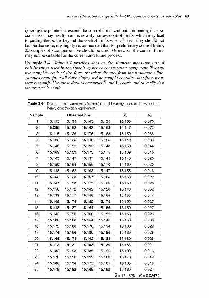
Phase I (Detecting Large Shifts)—SPC: Control Charts for Variables 63
ignoring the points that exceed the control limits without eliminating the spe-cial causes may result in unnecessarily narrow control limits, which may lead to putting the points beyond the control limits when, in fact, they should not be. Furthermore, it is highly recommended that for preliminary control limits, 25 samples of size four or five should be used. Otherwise, the control limits may not be suitable for the current and future process.
Example 3.4 Table 3.4 provides data on the diameter measurements of ball bearings used in the wheels of heavy construction equipment. Twenty- five samples, each of size four, are taken directly from the production line. Samples come from all three shifts, and no sample contains data from more than one shift. Use these data to construct X– and R charts and to verify that the process is stable.
Table 3.4 Diameter measurements (in mm) of ball bearings used in the wheels of heavy construction equipment.
Sample Observations x–i Ri
1 15.155 15.195 15.145 15.125 15.155 0.070
2 15.095 15.162 15.168 15.163 15.147 0.073
3 15.115 15.126 15.176 15.183 15.150 0.068
4 15.122 15.135 15.148 15.155 15.140 0.033
5 15.148 15.152 15.192 15.148 15.160 0.044
6 15.169 15.159 15.173 15.175 15.169 0.016
7 15.163 15.147 15.137 15.145 15.148 0.026
8 15.150 15.164 15.156 15.170 15.160 0.020
9 15.148 15.162 15.163 15.147 15.155 0.016
10 15.152 15.138 15.167 15.155 15.153 0.029
11 15.147 15.158 15.175 15.160 15.160 0.028
12 15.158 15.172 15.142 15.120 15.148 0.052
13 15.133 15.177 15.145 15.165 15.155 0.044
14 15.148 15.174 15.155 15.175 15.155 0.027
15 15.143 15.137 15.164 15.156 15.150 0.027
16 15.142 15.150 15.168 15.152 15.153 0.026
17 15.132 15.168 15.154 15.146 15.150 0.036
18 15.172 15.188 15.178 15.194 15.183 0.022
19 15.174 15.166 15.186 15.194 15.180 0.028
20 15.166 15.178 15.192 15.184 15.180 0.026
21 15.172 15.187 15.193 15.180 15.183 0.021
22 15.182 15.198 15.185 15.195 15.190 0.016
23 15.170 15.150 15.192 15.180 15.173 0.042
24 15.186 15.194 15.175 15.185 15.185 0.019
25 15.178 15.192 15.168 15.182 15.180 0.024–x– = 15.1628 R
– = 0.03479
H1277 ch03.indd 63H1277 ch03.indd 63 3/8/07 5:39:02 PM3/8/07 5:39:02 PM
64 Chapter Three
Solution: From Table A.2 for a sample of size n = 4, we have D3 = 0 and D4 = 2.282. Thus, the control limits for the R chart are
LCL
UCL
= = × =
= = × =
D R
D R
3
4
0 0 03479 0
2 282 0 03479 0
. ,
. . .. .07936
It is customary to prepare the R chart first and verify that all the plotted points fall within the control limits, and only then proceed to construct the X
– chart. In
fact, the concept of bringing the process variability under control first and then proceeding to control the average does make a lot of sense. This is because it is almost impossible to bring the process average under control without control-ling the process variability.
The R chart for the preceding data is given in Figure 3.10, which shows that all the plotted points fall within the control limits and that there is no evidence of any special pattern. Therefore, we may conclude that the only variation present in the process is due to common causes. In this case, we can proceed to calculate the control limits for the X
– chart. From Table A.2 for a
sample of size n = 4, we get A2 = 0.729. We have
LCL
UC
= − = − × =x A R2 15 1628 0 729 0 03479 15 13746. . . . ,
LL = + = + × =x A R2 15 1628 0 729 0 03479 15 18814. . . . .
The X– chart for these data is given in Figure 3.10, which shows that point 22
exceeds the UCL. Moreover, there are too many consecutive points that fall below the CL. This indicates that the process is not under control and that there are some special causes present that are affecting the process average. A thorough investigation should be launched to find the special causes, and appropriate action should be taken to eliminate them before recalculating the control limits for an ongoing process.
A process is considered out of control not only when the points exceed the control limits, but also when the points show patterns of nonrandomness. The Western Electric Statistical Quality Control Handbook (1956, 27) gives a set of decision rules for determining nonrandom patterns on control charts. In particular, it suggests the patterns are nonrandom if:
1. Two out of three successive points exceed the 2σ warning limits
2. Four out of five successive points fall at a distance of 1σ or beyond from the CL
3. Eight successive points fall on one side of the CL
4. Seven successive points run either upward or downward
3.3.1.1 Interpretation of Shewhart X– and R Control Charts
We should investigate any out- of-control points—that is, points on or beyond the 3σ control limits—or any patterns of nonrandomness on the R chart before interpreting the X
– chart. As discussed earlier, the reason for doing this is sim-
ple. It is not possible to bring the average under control without first bringing
H1277 ch03.indd 64H1277 ch03.indd 64 3/8/07 5:39:02 PM3/8/07 5:39:02 PM
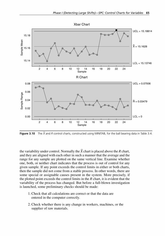
Phase I (Detecting Large Shifts)—SPC: Control Charts for Variables 65
the variability under control. Normally the X– chart is placed above the R chart,
and they are aligned with each other in such a manner that the average and the range for any sample are plotted on the same vertical line. Examine whether one, both, or neither chart indicates that the process is out of control for any given sample. If any point exceeds the control limits in either or both charts, then the sample did not come from a stable process. In other words, there are some special or assignable causes present in the system. More precisely, if the plotted point exceeds the control limits in the R chart, it is evident that the variability of the process has changed. But before a full- blown investigation is launched, some preliminary checks should be made:
1. Check that all calculations are correct or that the data are entered in the computer correctly.
2. Check whether there is any change in workers, machines, or the supplier of raw materials.
15.14
15.16
15.18
24222018161412108642
0.00
0.04
0.08
0.06
0.02
24222018161412108642
UCL = 15.18814
X = 15.1628
LCL = 15.13746
UCL = 0.07936
R = 0.03479
LCL = 0
Sample
Sample
R Chart
Xbar ChartS
ampl
e R
ange
Sam
ple
Mea
n
Figure 3.10 The X– and R control charts, constructed using MINITAB, for the ball bearing data in Table 3.4.
H1277 ch03.indd 65H1277 ch03.indd 65 3/8/07 5:39:02 PM3/8/07 5:39:02 PM
66 Chapter Three
If the points exceed the control limits in the X– chart, then the process mean
has changed. Again, follow the preliminary checks before launching an investigation.
If points exceed the limits in both the X– chart and the R chart, this usually
indicates that a sudden shift has occurred in the lot from which the samples were taken. In such cases, after making the preliminary checks, there should be an investigation concentrating on the period during which that lot was produced. Depending on the process, stopping production until the special causes are detected should be considered.
In addition to points exceeding the control limits, nonrandom patterns such as a run of seven points moving upward or downward, or a run of eight successive points falling above or below the CL should be checked.
An upward run or a run above the CL in an R chart indicates:
1. A greater variability or a tendency of perpetuating a greater variability in the output of the process is occurring. This may be due to new material of undesirable low quality or a difference between the shifts. Immediate attention to detect special causes is warranted.
2. The measurement system has changed.
A downward run or a run below the CL in an R chart indicates:
1. A smaller variability or a tendency of perpetuating a smaller variability in the output of the process is occurring. This is usually a good sign for the process. A thorough investigation should be made so that similar conditions are maintained as long as possible. Similar conditions should be implemented elsewhere in the process.
2. The measurement system has changed.
A run relative to an X– chart indicates:
1. The process average has changed or is still changing.
2. The measurement system has changed.
3.3.1.2 Extending the Current Control Limits for Future Control
If current data from at least 25 sample periods are contained within the cur-rent control limits, we may use these limits to cover future periods. However, these limits are used for future periods on the condition that immediate action will be taken if any out- of-control indication appears or if the points consis-tently fall very close to the CL. The latter case indicates that the process has improved and that new control limits should be recalculated. Again, note that in any case, control limits for future use should be extended for only 25 to 30 sample periods at a time.
It is pertinent to note that a change in sample size will affect the control limits for both the X
– chart and the R chart; therefore, whenever there is a
H1277 ch03.indd 66H1277 ch03.indd 66 3/8/07 5:39:02 PM3/8/07 5:39:02 PM
Phase I (Detecting Large Shifts)—SPC: Control Charts for Variables 67
change in sample size, new control limits should be recalculated. This situa-tion may arise if it is decided to take smaller samples more frequently, which usually is the case when one wants to catch larger shifts (larger than 1.5σ) without increasing the total number of parts sampled over the whole sam-pling period. Another scenario is when it is decided to increase the sample size but sample less frequently, which usually is the case when one wants to catch smaller shifts (shifts of 1.5σ or smaller). To recalculate the new control limits, proceed as follows:
1. Estimate the process standard deviation using the existing sample size
ˆ ,σ =
R
d2 (3.14)
where R– is the sample range average for the period with ranges
in control, and the value of d2 is found in Table A.2 for the existing sample size.
2. Using the values for d2, D3, D4, and A2 from Table A.2 for the new sample size, calculate the new range and control limits as follows:
Estimate the new sample range average, that is,
R dnew = ×2 ˆ .σ (3.15)
Then the new control limits for the X– control chart are
LCL
CL
UCL
= − ×
=
= + ×
x A R
x
x A R
2
2
new
new
,
,
,
(3.16)
and the new control limits for the R control chart are
LCL
CL
UCL
= ×
=
= ×
D R
R
D R
3
4
new
new
new
,
,
.
(3.17)
Example 3.5 To illustrate the technique of calculating the new control lim-its, consider the X
– and R control charts developed for the ball bearing data
in Example 3.4. The charts in Figure 3.10 are based on a sample size of four. Because one point in the X
– chart exceeded the control limit, there may be
a small shift in the process mean. Thus, the Six Sigma Green Belt wants to increase the sample size to six. Determine the control limits required for the new samples of size six for both the X
– chart and the R chart.
Solution: From Table A.2 for n = 4, d2 = 2.059. From Example 3.4 and using equation (3.14), we have
H1277 ch03.indd 67H1277 ch03.indd 67 3/8/07 5:39:03 PM3/8/07 5:39:03 PM
68 Chapter Three
ˆ .
.. .σ = = =
R
d2
0 03479
2 0590 0169
Again, from Table A.2 for n = 6, d2 = 2.534. Using equation (3.15), we have
Rnew = × =2 534 0 0169 0 0428246. . . .
The new control limits for the X– control chart for samples of size six are
LCL
CL
= − × =
=
15 1628 0 483 0 0428246 15 1421
15 1
. . . . ,
. 6628
15 1628 0 483 0 0428246 15 18348
,
. . . . .UCL = + × =
The new control limits for the R control chart for samples of size six are
LCL
CL
UCL
= × =
=
= ×
0 0 0428246 0
0 0428246
2 004 0
. ,
. ,
. .00428246 0 08582= . .
Note that the net result of increasing the sample size is to narrow the control limits for the X
– chart and to move the CL and the control limits for the R chart
higher. This is because the expected range value for the larger sample increases. In this example, however, the LCL for the R chart remains the same because the value of D3 for sample sizes four and six is zero.
3.3.2 Shewhart X– and R Control Charts When Process
Mean and Process Standard Deviation Are Known
If the process mean µ and the process standard deviation σ are known, then the X
– chart and the R chart are developed as follows:
Step 1. Calculate x–i and Ri for the ith sample for i = 1, 2, 3, . . . , m, where m is the number of samples collected during the study period.
Step 2. Calculate the control limits for the X– control chart
UCL = µ
σ+ 3n
,
(3.18)
CL = µ, (3.19)
LCL = µ
σ− 3n
.
(3.20)
Note: Instead of calculating 3σ limits, we can also calculate the probability limits at the desired level of significance α simply by replacing 3 with zα/2 in equations (3.18) and (3.20).
H1277 ch03.indd 68H1277 ch03.indd 68 3/8/07 5:39:03 PM3/8/07 5:39:03 PM
Phase I (Detecting Large Shifts)—SPC: Control Charts for Variables 69
Step 3. Calculate the control limits for the R control chart.
Recalling that σ = R/d2 and σR = d3σ, we have
UCL = d
d d
d d
D
R2
2 3
2 3
2
3
3
3
σ σ
σ σ
σ
σ
+
= +
= +
=
( )
,
(3.21)
CL = σ, (3.22)
LCL = d
d d
d d
D
R2
2 3
2 3
1
3
3
3
σ σ
σ σ
σ
σ
−
= −
= −
=
( )
,
(3.23)
where the values of D1 and D2 for various sample sizes are given in Table A.2.
3.3.3 Shewhart Control Chart for Individual Observations
Sometimes it is necessary to study SPC using individual observations only because it may not be feasible to form rational subgroups of size greater than one. This scenario, for example, would arise when:
1. Sampling is very expensive and it is not economical to take samples of size greater than one.
2. Observations are collected through experimentation and it may take several days or weeks to take one observation.
3. The circumstances warrant that each unit must be inspected or the process is completely automated, so that the measurement on each observation can be taken without much extra expense.
4. Only a few units are produced each day and the difference is between the units and not within the units, so one observation from each unit is sufficient.
5. Sampling is destructive and the units are very expensive. For example, certain bulbs for projectors are very expensive. If we want to study the life of such bulbs, then collecting the data will cause the bulbs to be destroyed.
The control charts for individual observations are very similar to X– and R con-
trol charts. However, in the case of individual observations, because the sam-ple contains only one observation, it is not possible to find the sample range in the usual manner. Instead, we find the sample range as the absolute difference between the two successive observations. This type of sample range is usually known as the moving range (MR), that is,
H1277 ch03.indd 69H1277 ch03.indd 69 3/8/07 5:39:03 PM3/8/07 5:39:03 PM
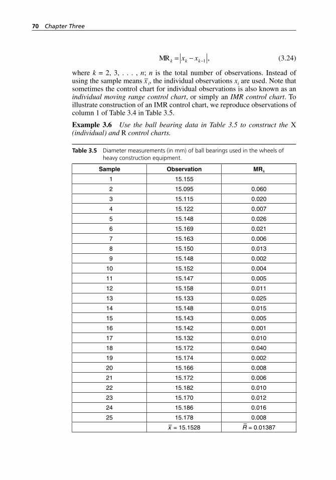
70 Chapter Three
MRk k kx x= − −1 ,
(3.24)
where k = 2, 3, . . . , n; n is the total number of observations. Instead of using the sample means x–i, the individual observations xi are used. Note that sometimes the control chart for individual observations is also known as an individual moving range control chart, or simply an IMR control chart. To illustrate construction of an IMR control chart, we reproduce observations of column 1 of Table 3.4 in Table 3.5.
Example 3.6 Use the ball bearing data in Table 3.5 to construct the X (individual) and R control charts.
Table 3.5 Diameter measurements (in mm) of ball bearings used in the wheels of heavy construction equipment.
Sample Observation MRk
1 15.155
2 15.095 0.060
3 15.115 0.020
4 15.122 0.007
5 15.148 0.026
6 15.169 0.021
7 15.163 0.006
8 15.150 0.013
9 15.148 0.002
10 15.152 0.004
11 15.147 0.005
12 15.158 0.011
13 15.133 0.025
14 15.148 0.015
15 15.143 0.005
16 15.142 0.001
17 15.132 0.010
18 15.172 0.040
19 15.174 0.002
20 15.166 0.008
21 15.172 0.006
22 15.182 0.010
23 15.170 0.012
24 15.186 0.016
25 15.178 0.008
x– = 15.1528 R– = 0.01387
H1277 ch03.indd 70H1277 ch03.indd 70 3/8/07 5:39:03 PM3/8/07 5:39:03 PM
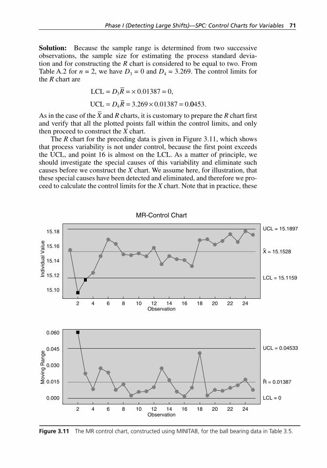
Phase I (Detecting Large Shifts)—SPC: Control Charts for Variables 71
Solution: Because the sample range is determined from two successive observations, the sample size for estimating the process standard devia-tion and for constructing the R chart is considered to be equal to two. From Table A.2 for n = 2, we have D3 = 0 and D4 = 3.269. The control limits for the R chart are
LCL
UCL
= = × =
= = × =
D R
D R
3
4
0 01387 0
3 269 0 01387 0
. ,
. . .00453.
As in the case of the X– and R charts, it is customary to prepare the R chart first
and verify that all the plotted points fall within the control limits, and only then proceed to construct the X chart.
The R chart for the preceding data is given in Figure 3.11, which shows that process variability is not under control, because the first point exceeds the UCL, and point 16 is almost on the LCL. As a matter of principle, we should investigate the special causes of this variability and eliminate such causes before we construct the X chart. We assume here, for illustration, that these special causes have been detected and eliminated, and therefore we pro-ceed to calculate the control limits for the X chart. Note that in practice, these
15.14
15.12
15.10
15.16
15.18
24222018161412108642
0.000
0.030
0.060
0.045
0.015
24222018161412108642
UCL = 15.1897
X = 15.1528
LCL = 15.1159
UCL = 0.04533
R = 0.01387
LCL = 0
Observation
Observation
MR-Control Chart
Mov
ing
Ran
geIn
divi
dual
Val
ue
Figure 3.11 The MR control chart, constructed using MINITAB, for the ball bearing data in Table 3.5.
H1277 ch03.indd 71H1277 ch03.indd 71 3/8/07 5:39:03 PM3/8/07 5:39:03 PM
72 Chapter Three
observations should be ignored after detecting and eliminating the special causes, and the control limits should be recalculated. Again, from Table A.2 for a sample of size n = 2, we get d2 = 1.128. Thus, we have
LCL = − = − = − =x xR
d3 3 15 1528 3
0 01387
1 12815 1
2
ˆ ..
..σ 1159
3 3 15 1528 30 01387
1 1282
,
ˆ ..
.UCL = + = + = +x x
R
dσ == 15 1897. .
Notice, however, there is little difference in how we compute the control limits for the X
– chart and the X chart. For calculating the control limits of the
X chart, we always use sample size n = 1. In other words, we do not use the sample size n = 2 or the control limits as x ± 3 2σ ; rather, we simply use the control limits as x ± 3σ because n = 2 is used only for determining the control limits of the R chart and for estimating σ. The X chart for the preced-ing data is given in Figure 3.11, which shows that points 2 and 3 fall below the LCL. Moreover, there are too many consecutive points that fall above the CL. This indicates that the process is not under control and that there are some special causes present that are affecting the process average. Therefore, a thorough investigation should be launched to find the special causes, and appropriate action should be taken to eliminate them.
Note: There are some limitations of using Shewhart charts for individual observations. If the process characteristic is nonnormal, the rules applicable to the X
– chart may not hold for the X chart, because x– usually behaves like nor-
mal as a result of the central limit theorem, even if the process distribution is not normal. This would not be true for individual observations. Therefore, in such cases the X charts may give signals of special causes when they are not actually present. Also, note that the ranges are not independent, because the two adjacent ranges have a common point. Hence a run of successive points falling near or beyond the control limits does not have the same significance as in an ordinary control chart. For more detailed discussion on this topic, we recommend Montgomery (2005b), an excellent source.
3.3.4 Shewhart X– and S Control Charts
The X– and S control charts, similar to the X
– and R control charts, are devel-
oped from measured process output data, and both X– and S charts are used
together. The standard deviation s is usually a more efficient indicator of pro-cess variability than the range, particularly when the sample sizes are large (10 or greater). The sample standard deviation s for the S chart is calculated using all the data points rather than just the maximum and minimum values in a data set, as is done for the R chart. S charts are usually preferred over R charts when:
The sample is of size 10 or larger
The sample size is variable
The process is automated so the s for each sample can be easily calculated
•
•
•
H1277 ch03.indd 72H1277 ch03.indd 72 3/8/07 5:39:04 PM3/8/07 5:39:04 PM
Phase I (Detecting Large Shifts)—SPC: Control Charts for Variables 73
The sample standard deviation s is determined using the formula
sn
xn
xi ii
n
i
n
=1
1
12
1
2
1−−
⎛
⎝⎜⎞
⎠⎟⎛
⎝⎜⎜
⎞
⎠⎟⎟==
∑∑ .
(3.25)
The control limits for the X– and S control charts are determined as shown in
the following section.
Calculation of Control Limits
Step 1. First, calculate x–i and si for the ith sample, for i = 1, 2, 3, . . . , m, where m is the number of samples collected during the study period.
Step 2. Calculate
s
s s s
mm=
+ + +1 2 ...,
(3.26)
x
x x x
mm=
+ + +1 2 ....
(3.27)
Step 3. Calculate the control limits for the X– chart
UCL = xn
xs
c n
x A s
+
= +
= +
3
34
3
ˆ
,
σ
(3.28)
CL = x , (3.29)
LCL = xn
xs
c n
x A s
−
= −
= −
3
34
3
ˆ
,
σ
(3.30)
where the values of A3 and c4 for various sample sizes are given in Table A.2.Note: Instead of calculating 3σ limits, we can also calculate the probabil-
ity limits at the desired level of significance α simply by replacing 3 with zα/2 in equations (3.24) and (3.25). Thus, the control limits will be
UCL = x zn
x zs
c n
+
= +
α
α
σ/
/
ˆ
,
2
24
(3.31)
H1277 ch03.indd 73H1277 ch03.indd 73 3/8/07 5:39:04 PM3/8/07 5:39:04 PM
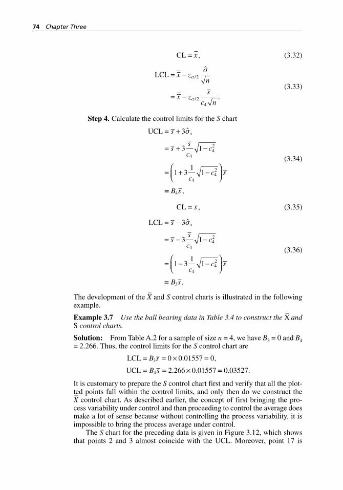
74 Chapter Three
CL = x , (3.32)
LCL = x zn
x zs
c n
−
= −
α
α
σ/
/
ˆ
.
2
24
(3.33)
Step 4. Calculate the control limits for the S chart
UCL = s
ss
cc
cc s
s+
= + −
= + −⎛⎝⎜
⎞⎠⎟
3
3 1
1 31
1
442
442
σ
== B s4 ,
(3.34)
CL = s , (3.35)
LCL = s
ss
cc
cc s
s−
= − −
= − −⎛⎝⎜
⎞⎠⎟
3
3 1
1 31
1
442
442
σ
== B s3 .
(3.36)
The development of the X–
and S control charts is illustrated in the following example.
Example 3.7 Use the ball bearing data in Table 3.4 to construct the X– and
S control charts.
Solution: From Table A.2 for a sample of size n = 4, we have B3 = 0 and B4 = 2.266. Thus, the control limits for the S control chart are
LCL =
UCL
B s
B s
3
4
0 0 01557 0
2 266 0 01557
= × =
= = ×
. ,
. . == 0 03527. .
It is customary to prepare the S control chart first and verify that all the plot-ted points fall within the control limits, and only then do we construct the X– control chart. As described earlier, the concept of first bringing the pro-
cess variability under control and then proceeding to control the average does make a lot of sense because without controlling the process variability, it is impossible to bring the process average under control.
The S chart for the preceding data is given in Figure 3.12, which shows that points 2 and 3 almost coincide with the UCL. Moreover, point 17 is
H1277 ch03.indd 74H1277 ch03.indd 74 3/8/07 5:39:04 PM3/8/07 5:39:04 PM
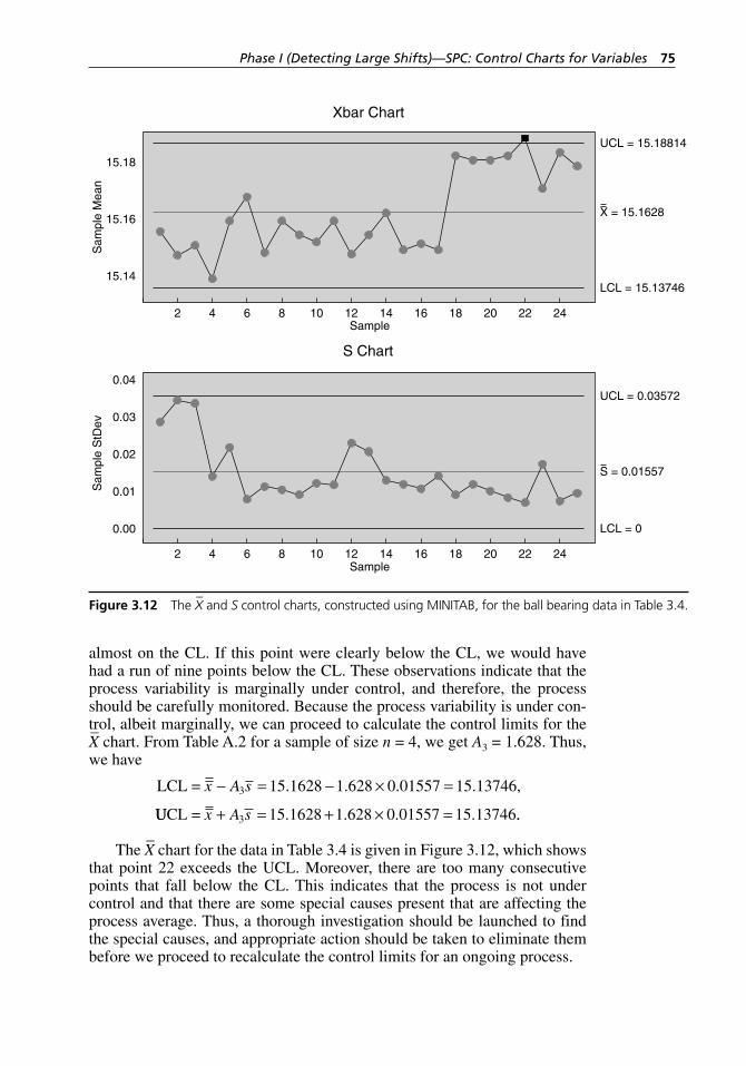
Phase I (Detecting Large Shifts)—SPC: Control Charts for Variables 75
almost on the CL. If this point were clearly below the CL, we would have had a run of nine points below the CL. These observations indicate that the process variability is marginally under control, and therefore, the process should be carefully monitored. Because the process variability is under con-trol, albeit marginally, we can proceed to calculate the control limits for the X– chart. From Table A.2 for a sample of size n = 4, we get A3 = 1.628. Thus,
we have
LCL = x A s− = − × =3 15 1628 1 628 0 01557 15 13746. . . . ,
UUCL = x A s+ = + × =3 15 1628 1 628 0 01557 15 13746. . . . ..
The X– chart for the data in Table 3.4 is given in Figure 3.12, which shows
that point 22 exceeds the UCL. Moreover, there are too many consecutive points that fall below the CL. This indicates that the process is not under control and that there are some special causes present that are affecting the process average. Thus, a thorough investigation should be launched to find the special causes, and appropriate action should be taken to eliminate them before we proceed to recalculate the control limits for an ongoing process.
15.14
15.16
15.18
24222018161412108642
0.00
0.02
0.04
0.03
0.01
24222018161412108642
UCL = 15.18814
X = 15.1628
LCL = 15.13746
UCL = 0.03572
S = 0.01557
LCL = 0
Sample
Sample
S Chart
Xbar ChartS
ampl
e S
tDev
Sam
ple
Mea
n
Figure 3.12 The X– and S control charts, constructed using MINITAB, for the ball bearing data in Table 3.4.
H1277 ch03.indd 75H1277 ch03.indd 75 3/8/07 5:39:04 PM3/8/07 5:39:04 PM
76 Chapter Three
3.3.4.1 Shewhart X– and S Control Charts
When Sample Size Is Variable
Sometimes it is not possible to select samples of the same size. In such cases we construct the X
– and S control charts by using the weighted mean –x– and the
square root of the pooled estimator s2 of σ2 as the CLs for the X– and S charts,
respectively. The upper and lower control limits are calculated for individual samples. For example, if the sample sizes are n1, n2, n3, . . . , nm, then the weighted mean –x– and the pooled estimator s2 are given by
x
n x
n
n x
N
i ii
m
ii
m
i ii
m
= ==
=
=∑
∑
∑1
1
1 ,
(3.37)
s s
n s
n
n si ii
m
ii
m
i ii= =
−
−=
−=
=
=∑
∑2
2
1
1
2
1
1
1
1( )
( )
( )mm
N m
∑−
,
(3.38)
where N = n1 + n2 + n3 + . . . + nm; m is the number of samples selected during the study period.
The control limits for the X– and S charts are given by
UCLx ix A s= + 3 , (3.39)
LCLx ix A s= − 3 , (3.40)
and
UCLs is B s= + 4 , (3.41)
LCLs is B s= − 3 , (3.42)
respectively. The values A3, B3, and B4 depend on the individual sample sizes. To illustrate the development of these charts, we use the data presented in Example 3.8.
Example 3.8 A manufacturing process produces piston rings with a fin-ished inside diameter of 9 centimeters and a standard deviation of 0.03 cen-timeter. From this process, 30 samples of variable sizes are carefully selected so that no sample comes from two machines or two shifts. In other words, every effort is made to ensure that no sample masks any special causes. The data are shown in Table 3.6. Construct X
– and S control charts for these data
H1277 ch03.indd 76H1277 ch03.indd 76 3/8/07 5:39:04 PM3/8/07 5:39:04 PM
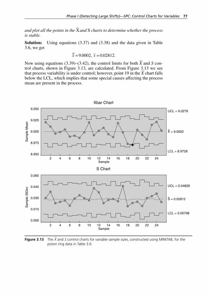
Phase I (Detecting Large Shifts)—SPC: Control Charts for Variables 77
and plot all the points in the X– and S charts to determine whether the process
is stable.
Solution: Using equations (3.37) and (3.38) and the data given in Table 3.6, we get
x s= =9 0002 0 02812. , . .
Now using equations (3.39)–(3.42), the control limits for both X– and S con-
trol charts, shown in Figure 3.13, are calculated. From Figure 3.13 we see that process variability is under control; however, point 19 in the X
– chart falls
below the LCL, which implies that some special causes affecting the process mean are present in the process.
9.000
8.975
8.950
9.025
9.050
24222018161412108642
0.000
0.030
0.060
0.045
0.015
24222018161412108642
UCL = 9.0276
LCL = 8.9728
UCL = 0.04826
LCL = 0.00798
X = 9.0002
S = 0.02812
Sample
Sample
S Chart
Xbar Chart
Sam
ple
StD
evS
ampl
e M
ean
Figure 3.13 The X– and S control charts for variable sample sizes, constructed using MINITAB, for the
piston ring data in Table 3.6.
H1277 ch03.indd 77H1277 ch03.indd 77 3/8/07 5:39:05 PM3/8/07 5:39:05 PM
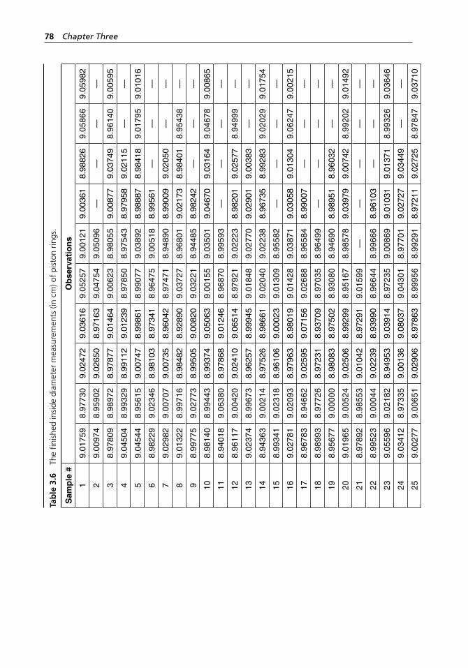
78 Chapter Three
Tab
le 3
.6
The
finis
hed
insi
de d
iam
eter
mea
sure
men
ts (i
n cm
) of
pist
on r
ings
.
Sam
ple
#O
bse
rvat
ion
s
19.
0175
98.
9773
09.
0247
29.
0361
69.
0525
79.
0012
19.
0036
18.
9882
69.
0586
69.
0598
2
29.
0097
48.
9590
29.
0265
08.
9716
39.
0475
49.
0509
6—
——
—
38.
9780
98.
9897
28.
9787
79.
0146
49.
0062
38.
9805
59.
0087
79.
0374
98.
9614
09.
0059
5
49.
0450
48.
9932
98.
9911
29.
0123
98.
9785
08.
9754
38.
9795
89.
0211
5—
—
59.
0454
48.
9561
59.
0074
78.
9986
18.
9907
79.
0389
28.
9888
78.
9841
89.
0179
59.
0101
6
68.
9822
99.
0234
68.
9810
38.
9734
18.
9647
59.
0051
88.
9956
1—
——
79.
0298
29.
0070
79.
0073
58.
9604
28.
9747
18.
9489
08.
9900
99.
0205
0—
—
89.
0132
28.
9971
68.
9848
28.
9289
09.
0372
78.
9680
19.
0217
38.
9840
18.
9543
8—
98.
9977
59.
0277
38.
9950
59.
0082
09.
0322
18.
9448
58.
9824
2—
——
108.
9814
08.
9944
38.
9937
49.
0506
39.
0015
59.
0350
19.
0467
09.
0316
49.
0467
89.
0086
5
118.
9401
89.
0638
08.
9786
89.
0124
68.
9687
08.
9959
3—
——
—
128.
9611
79.
0042
09.
0241
09.
0651
48.
9792
19.
0222
38.
9820
19.
0257
78.
9499
9—
139.
0237
48.
9967
38.
9625
78.
9994
59.
0184
89.
0277
09.
0290
19.
0038
3—
—
148.
9436
39.
0021
48.
9752
68.
9866
19.
0204
09.
0223
88.
9673
58.
9928
39.
0202
99.
0175
4
158.
9934
19.
0231
88.
9610
69.
0002
39.
0130
98.
9558
2—
——
—
169.
0278
19.
0209
38.
9796
38.
9801
99.
0142
89.
0387
19.
0305
89.
0130
49.
0624
79.
0021
5
178.
9678
38.
9466
29.
0259
59.
0715
69.
0268
88.
9658
48.
9900
7—
——
188.
9899
38.
9772
68.
9723
18.
9370
98.
9703
58.
9649
9—
——
—
198.
9567
79.
0000
08.
9808
38.
9750
28.
9308
08.
9469
08.
9895
18.
9603
2—
—
209.
0196
59.
0052
49.
0250
68.
9929
98.
9516
78.
9857
89.
0397
99.
0074
28.
9920
29.
0149
2
218.
9789
28.
9855
39.
0104
28.
9729
19.
0159
9—
——
——
228.
9952
39.
0004
49.
0223
98.
9399
08.
9664
48.
9966
68.
9610
3—
——
239.
0559
69.
0218
28.
9495
39.
0391
48.
9723
59.
0086
99.
0103
19.
0137
18.
9932
69.
0364
6
249.
0341
28.
9733
59.
0013
69.
0803
79.
0430
18.
9770
19.
0272
79.
0344
9—
—
259.
0027
79.
0065
19.
0290
68.
9786
38.
9995
68.
9929
18.
9721
19.
0272
58.
9784
79.
0371
0
H1277 ch03.indd 78H1277 ch03.indd 78 3/8/07 5:39:05 PM3/8/07 5:39:05 PM
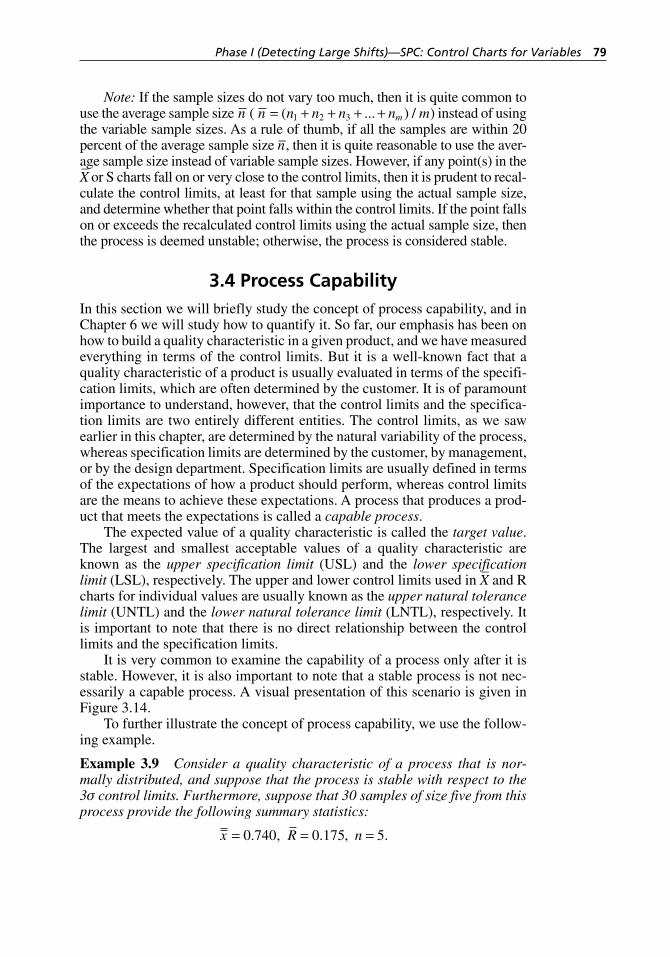
Phase I (Detecting Large Shifts)—SPC: Control Charts for Variables 79
Note: If the sample sizes do not vary too much, then it is quite common to use the average sample size n n n n n n mm( ( ... ) /= + + + +1 2 3 ) instead of using the variable sample sizes. As a rule of thumb, if all the samples are within 20 percent of the average sample size n–, then it is quite reasonable to use the aver-age sample size instead of variable sample sizes. However, if any point(s) in the X– or S charts fall on or very close to the control limits, then it is prudent to recal-
culate the control limits, at least for that sample using the actual sample size, and determine whether that point falls within the control limits. If the point falls on or exceeds the recalculated control limits using the actual sample size, then the process is deemed unstable; otherwise, the process is considered stable.
3.4 Process CapabilityIn this section we will briefly study the concept of process capability, and in Chapter 6 we will study how to quantify it. So far, our emphasis has been on how to build a quality characteristic in a given product, and we have measured everything in terms of the control limits. But it is a well- known fact that a quality characteristic of a product is usually evaluated in terms of the specifi-cation limits, which are often determined by the customer. It is of paramount importance to understand, however, that the control limits and the specifica-tion limits are two entirely different entities. The control limits, as we saw earlier in this chapter, are determined by the natural variability of the process, whereas specification limits are determined by the customer, by management, or by the design department. Specification limits are usually defined in terms of the expectations of how a product should perform, whereas control limits are the means to achieve these expectations. A process that produces a prod-uct that meets the expectations is called a capable process.
The expected value of a quality characteristic is called the target value. The largest and smallest acceptable values of a quality characteristic are known as the upper specification limit (USL) and the lower specification limit (LSL), respectively. The upper and lower control limits used in X
– and R
charts for individual values are usually known as the upper natural tolerance limit (UNTL) and the lower natural tolerance limit (LNTL), respectively. It is important to note that there is no direct relationship between the control limits and the specification limits.
It is very common to examine the capability of a process only after it is stable. However, it is also important to note that a stable process is not nec-essarily a capable process. A visual presentation of this scenario is given in Figure 3.14.
To further illustrate the concept of process capability, we use the follow-ing example.
Example 3.9 Consider a quality characteristic of a process that is nor-mally distributed, and suppose that the process is stable with respect to the 3σ control limits. Furthermore, suppose that 30 samples of size five from this process provide the following summary statistics:
x R n= = =0 740 0 175 5. , . , .
H1277 ch03.indd 79H1277 ch03.indd 79 3/8/07 5:39:05 PM3/8/07 5:39:05 PM
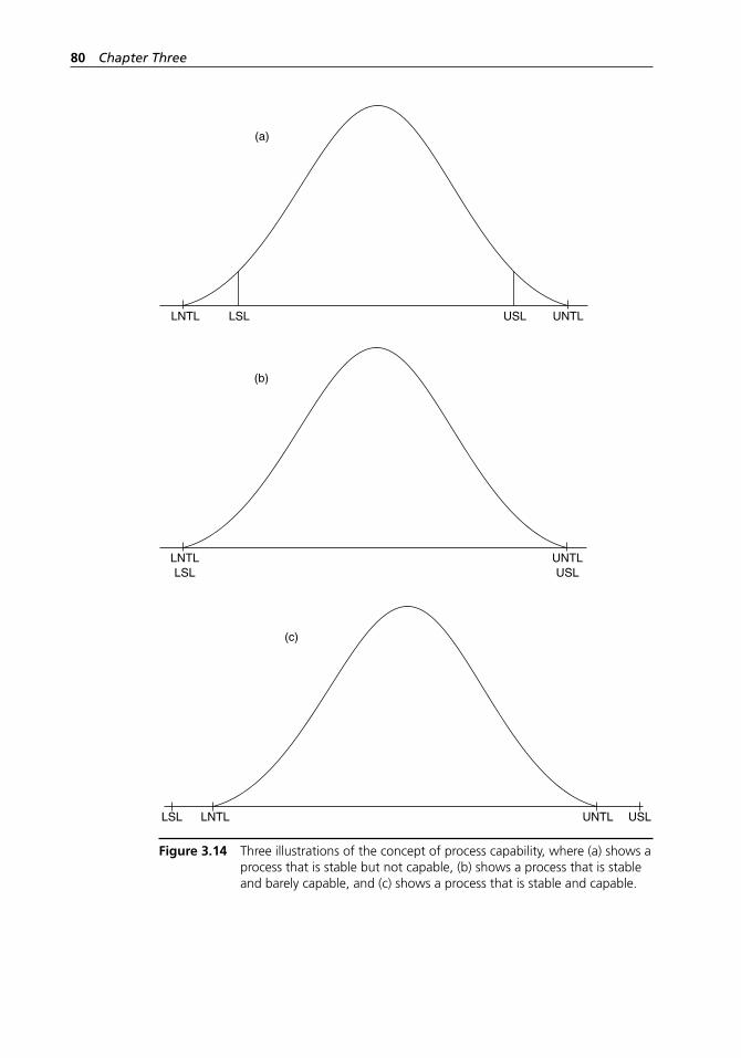
80 Chapter Three
(a)
LNTL LSL USL UNTL
Figure 3.14 Three illustrations of the concept of process capability, where (a) shows a process that is stable but not capable, (b) shows a process that is stable and barely capable, and (c) shows a process that is stable and capable.
(b)
LNTLLSL USL
UNTL
(c)
LNTLLSL USLUNTL
H1277 ch03.indd 80H1277 ch03.indd 80 3/8/07 5:39:05 PM3/8/07 5:39:05 PM
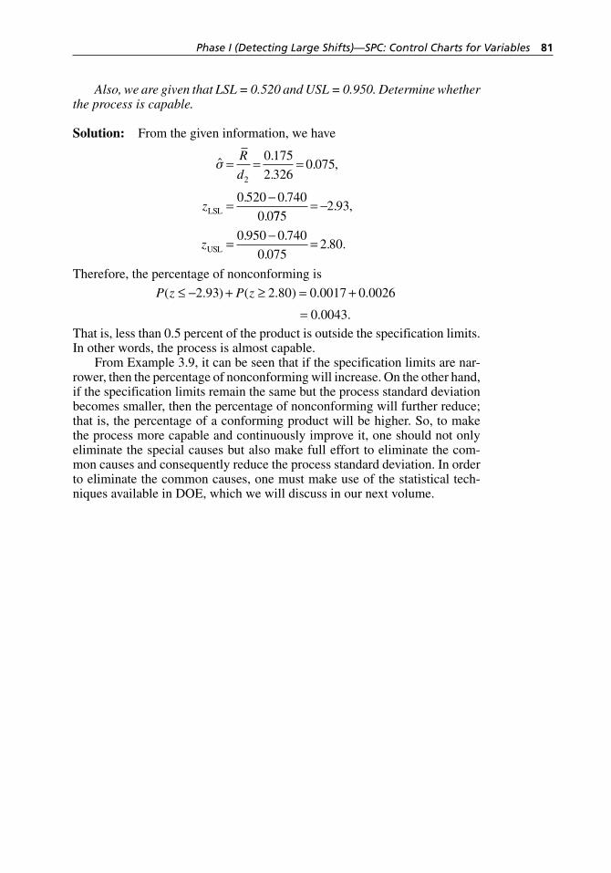
Phase I (Detecting Large Shifts)—SPC: Control Charts for Variables 81
Also, we are given that LSL = 0.520 and USL = 0.950. Determine whether the process is capable.
Solution: From the given information, we have
ˆ .
.. ,
. .
.
σ = = =
=−
R
d
z
2
0 175
2 3260 075
0 520 0 740
0 0LSL 7752 93
0 950 0 740
0 0752 80
= −
=−
=
. ,
. .
.. .zUSL
Therefore, the percentage of nonconforming is
P z P z( . ) ( . ) . .
. .
≤ − + ≥ = +
=
2 93 2 80 0 0017 0 0026
0 0043That is, less than 0.5 percent of the product is outside the specification limits. In other words, the process is almost capable.
From Example 3.9, it can be seen that if the specification limits are nar-rower, then the percentage of nonconforming will increase. On the other hand, if the specification limits remain the same but the process standard deviation becomes smaller, then the percentage of nonconforming will further reduce; that is, the percentage of a conforming product will be higher. So, to make the process more capable and continuously improve it, one should not only eliminate the special causes but also make full effort to eliminate the com-mon causes and consequently reduce the process standard deviation. In order to eliminate the common causes, one must make use of the statistical tech-niques available in DOE, which we will discuss in our next volume.
H1277 ch03.indd 81H1277 ch03.indd 81 3/8/07 5:39:05 PM3/8/07 5:39:05 PM

H1277 ch03.indd 82H1277 ch03.indd 82 3/8/07 5:39:05 PM3/8/07 5:39:05 PM
83
As noted in the previous chapter, quality characteristics are usually of two types: variables and attributes. In Chapter 3, we studied control charts for variables for detecting large shifts. However, not all qual-
ity characteristics can be numerically measured. For example, we may be interested in finding out whether the new- car paint meets the specifications in terms of shine, uniformity, and scratches. In this example we cannot quantify the shine, the blemishes, or the scratches. In other words, we cannot numeri-cally measure the shine, the uniformity, or the scratches; consequently, to study the quality of paint on new cars, we cannot use control charts for vari-ables. This type of situation sometimes arises when a quality characteristic is measurable, but because of cost, time, or both, we do not want to take the measurements. Rather, we may prefer to use a more economical method, such as a go or no- go gauge. Therefore, it is important that we study con-trol charts appropriate for quality characteristics that cannot be numerically measured. Such control charts are called control charts for attributes. In this chapter, we will study various control charts for attributes for detecting large shifts, which usually occur in phase I implementation of SPC.
4.1 Control Charts for Attributes
When a quality characteristic cannot be numerically measured, we classify such product as defective or nondefective. In SPC it has become more com-mon to use the terminology conforming or nonconforming instead of non-defective or defective. Throughout this book, we shall use conforming or nonconforming.
Definition 4.1 A quality characteristic that classifies any product as conforming or nonconforming is called an attribute.
4
Phase I (Detecting Large Shifts)—SPC: Control Charts for Attributes
H1277 ch04.indd 83H1277 ch04.indd 83 3/8/07 5:50:05 PM3/8/07 5:50:05 PM
84 Chapter Four
For instance, quality characteristics such as the determination that a soda can is not leaking, a stud has regular edges, a rod fits into a slot, a 100-watt lightbulb meets the desired standard, and a steel rivet meets the manufac-turer’s quality specifications are examples of attributes. Note that the data collected on a quality characteristic that is an attribute are simply count data. Moreover, the sample sizes when using control charts for attributes are nor-mally much larger (usually in the hundreds) than a sample of size four or five that we usually use in control charts for variables.
In general, variable control charts are more informative than attribute control charts. They are very effective in detecting a defect even before it occurs, whereas attribute control charts are used only after the defects have occurred. There are cases, however, when variable control charts have limitations. For example, consider a product that is nonconforming due to any one of 10 quality characteristics that do not conform to speci-fications. In this case we cannot control all 10 quality characteristics by using one variable control chart, because one variable control chart can control only one quality characteristic at a time. Therefore, to control all 10 quality characteristics, we will have to use 10 different variable con-trol charts. On the other hand, one attribute control chart can study all the quality characteristics because a nonconforming unit is nonconforming irrespective of the number of quality characteristics that do not conform to specifications. We can conclude that both variable and attribute control charts have pros and cons.
In some cases the quality characteristic is such that instead of classifying a unit as conforming or nonconforming, it records the number of nonconfor-mities per manufactured unit—for example, the number of holes in a roll of paper, the number of irregularities per unit area of a spool of cloth, the num-ber of blemishes on a painted surface, the number of loose ends in a circuit board, the number of nonconformities per unit length of a cable, the number of nonconformities of all types in an assembled unit, and so on. In such cases, we use control charts that fall under the category of control charts for attri-butes. These control charts are used to reduce the number of nonconformities per unit length, area, or volume of a single manufactured unit, or to reduce the number of nonconformities per manufactured or assembled unit.
The control charts for attributes are quite similar to the control charts for variables; that is, the CL and the control limits are set in the same manner as in the control charts for variables. However, it is important to note that the reasons for using control charts for variables and control charts for attri-butes are quite distinct. As noted in Chapter 3, the purpose of using control charts for variables in any process is to reduce the variability due to special or assignable causes, whereas control charts for attributes are used to moni-tor the number of nonconforming units, the number of nonconformities per manufactured or assembled unit, or simply the number of nonconformities per unit length, area, or volume of a single manufactured unit.
In this chapter, we will study four types of control charts for attributes: the p chart, the np chart, the c chart, and the u chart. Table 4.1 gives a very brief description of these charts, which can help determine the appropriate type of control chart for the quality characteristic under investigation.
H1277 ch04.indd 84H1277 ch04.indd 84 3/8/07 5:50:06 PM3/8/07 5:50:06 PM
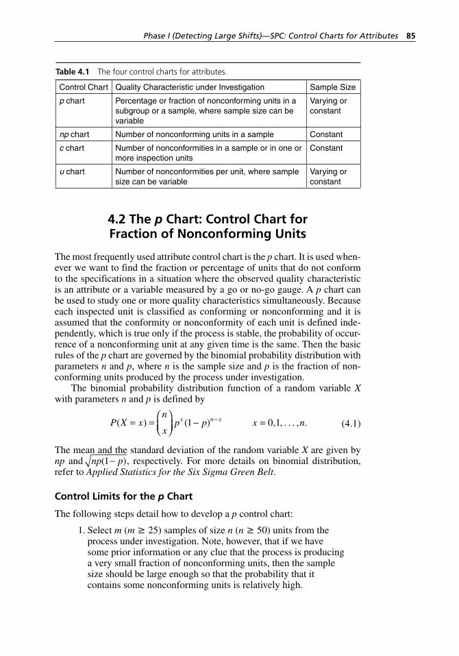
Phase I (Detecting Large Shifts)—SPC: Control Charts for Attributes 85
4.2 The p Chart: Control Chart for Fraction of Nonconforming Units
The most frequently used attribute control chart is the p chart. It is used when-ever we want to find the fraction or percentage of units that do not conform to the specifications in a situation where the observed quality characteristic is an attribute or a variable measured by a go or no- go gauge. A p chart can be used to study one or more quality characteristics simultaneously. Because each inspected unit is classified as conforming or nonconforming and it is assumed that the conformity or nonconformity of each unit is defined inde-pendently, which is true only if the process is stable, the probability of occur-rence of a nonconforming unit at any given time is the same. Then the basic rules of the p chart are governed by the binomial probability distribution with parameters n and p, where n is the sample size and p is the fraction of non-conforming units produced by the process under investigation.
The binomial probability distribution function of a random variable X with parameters n and p is defined by
P X xn
xp p x nx n x( ) ( ) , , . . . , .= =
⎛⎝⎜
⎞⎠⎟
− =−1 0 1
(4.1)
The mean and the standard deviation of the random variable X are given by np and np p( )1− , respectively. For more details on binomial distribution, refer to Applied Statistics for the Six Sigma Green Belt.
Control Limits for the p Chart
The following steps detail how to develop a p control chart:
1. Select m (m ≥ 25) samples of size n (n ≥ 50) units from the process under investigation. Note, however, that if we have some prior information or any clue that the process is producing a very small fraction of nonconforming units, then the sample size should be large enough so that the probability that it contains some nonconforming units is relatively high.
Table 4.1 The four control charts for attributes.
Control Chart Quality Characteristic under Investigation Sample Size
p chart Percentage or fraction of nonconforming units in a subgroup or a sample, where sample size can be variable
Varying or constant
np chart Number of nonconforming units in a sample Constant
c chart Number of nonconformities in a sample or in one or more inspection units
Constant
u chart Number of nonconformities per unit, where sample size can be variable
Varying or constant
H1277 ch04.indd 85H1277 ch04.indd 85 3/8/07 5:50:06 PM3/8/07 5:50:06 PM
86 Chapter Four
2. Find the number of nonconforming units in each sample.
3. Find the fraction pi of nonconforming units for each sample, that is,
p
x
ni = ,
(4.2)
where x is the number of nonconforming units in the ith (i = 1, 2, . . . , m) sample.
4. Find the average nonconforming p– over the m samples, that is,
p
p p p
mm=
+ + +1 2 ....
(4.3)
The value of p– determines the CL for the p chart and is an estimate of p, the process fraction of nonconforming units.
5. Using the well- known result that the binomial distribution with parameters n and p for large n can be approximated by the normal distribution with mean np and variance np(1–p), it can be seen that p– will be approximately normally distributed
with mean p and standard deviation p p
n
( )1−. Hence the
upper and lower 3σ control limits and the CL for the p chart are
UCL = +
−p
p p
n3
1( ),
(4.4)
CL = p, (4.5)
LCL = −
−p
p p
n3
1( ).
(4.6)
In equations (4.4) and (4.5), p p
n
( )1− is an estimator of
p p
n
( )1−, the stan-
dard deviation of p. Furthermore, if the control charts are being implemented for the first time, then the control limits given by equations (4.4)–(4.6) should be treated as the trial limits. In other words, before using these control limits any further, the points corresponding to all the samples used to determine these limits should be plotted and verified, and it should be established that all the points fall within these control limits and that there is no evident pat-tern present. If any sample points exceed the control limits or if there is any pattern, then the possible special causes should be detected and eliminated before recalculating the control limits for future use. When recalculating the control limits, points that exceeded the trial control limits should be ignored, provided any special causes related to such points have been detected and eliminated.
H1277 ch04.indd 86H1277 ch04.indd 86 3/8/07 5:50:06 PM3/8/07 5:50:06 PM

Phase I (Detecting Large Shifts)—SPC: Control Charts for Attributes 87
Note: Sometimes for small values of p–, n, or both, the value of the LCL may be negative. In such cases, we always set the LCL at zero because the fraction of nonconforming units can never go below zero.
Interpreting the Control Chart for Fraction Nonconforming
1. If any point or points exceed the upper or lower control limit, we conclude that the process is not stable and that some special causes are present in the process.
2. The presence of special causes, which may be favorable or unfavorable, must be investigated, and appropriate action(s) should be taken.
3. A point above the UCL is generally an indication that:
The control limit or the plotted point is in error.
The process performance has deteriorated or is deteriorating.
The measurement system has changed.
4. A point below the LCL is generally an indication that:
The control limit or the plotted point is in error.
The process performance has improved or is improving. This condition of the process should be investigated very carefully so that such conditions of improvement are implemented on a permanent basis at this location and elsewhere in the industry.
The measurement system has changed.
5. As in the case of X– and R charts, or X
– and S charts, the presence
of any unusual patterns or trends is either an indication of an unstable process or an advance warning of conditions that, if left unattended or without any appropriate action, could make the process unstable.
6. If p– is moderately high (np– ≥ 5), then an approximately equal number of points should fall on either side of the CL. Therefore, either of the following conditions could indicate that the process has shifted or a trend of a shift has started:
A run of seven or more points going up or going down.
A run of seven or more points falling below or above the CL.
7. A run above the CL or a run going up generally indicates that:
The process performance has deteriorated and may still be deteriorating.
The measurement system has changed.
8. A run below the CL or a run going down generally indicates that:
•
•
•
•
•
•
•
•
•
•
H1277 ch04.indd 87H1277 ch04.indd 87 3/8/07 5:50:06 PM3/8/07 5:50:06 PM
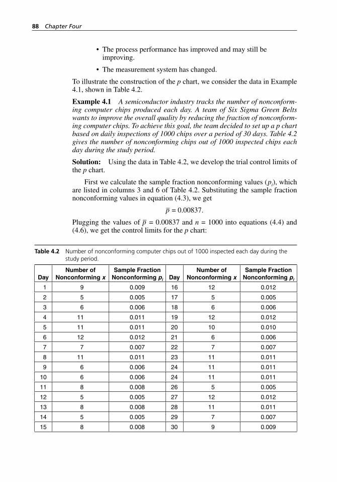
88 Chapter Four
The process performance has improved and may still be improving.
The measurement system has changed.
To illustrate the construction of the p chart, we consider the data in Example 4.1, shown in Table 4.2.
Example 4.1 A semiconductor industry tracks the number of nonconform-ing computer chips produced each day. A team of Six Sigma Green Belts wants to improve the overall quality by reducing the fraction of nonconform-ing computer chips. To achieve this goal, the team decided to set up a p chart based on daily inspections of 1000 chips over a period of 30 days. Table 4.2 gives the number of nonconforming chips out of 1000 inspected chips each day during the study period.
Solution: Using the data in Table 4.2, we develop the trial control limits of the p chart.
First we calculate the sample fraction nonconforming values (pi), which are listed in columns 3 and 6 of Table 4.2. Substituting the sample fraction nonconforming values in equation (4.3), we get
p– = 0.00837.
Plugging the values of p– = 0.00837 and n = 1000 into equations (4.4) and (4.6), we get the control limits for the p chart:
•
•
Table 4.2 Number of nonconforming computer chips out of 1000 inspected each day during the study period.
DayNumber of
Nonconforming xSample Fraction
Nonconforming pi DayNumber of
Nonconforming xSample Fraction
Nonconforming pi
1 9 0.009 16 12 0.012
2 5 0.005 17 5 0.005
3 6 0.006 18 6 0.006
4 11 0.011 19 12 0.012
5 11 0.011 20 10 0.010
6 12 0.012 21 6 0.006
7 7 0.007 22 7 0.007
8 11 0.011 23 11 0.011
9 6 0.006 24 11 0.011
10 6 0.006 24 11 0.011
11 8 0.008 26 5 0.005
12 5 0.005 27 12 0.012
13 8 0.008 28 11 0.011
14 5 0.005 29 7 0.007
15 8 0.008 30 9 0.009
H1277 ch04.indd 88H1277 ch04.indd 88 3/8/07 5:50:06 PM3/8/07 5:50:06 PM
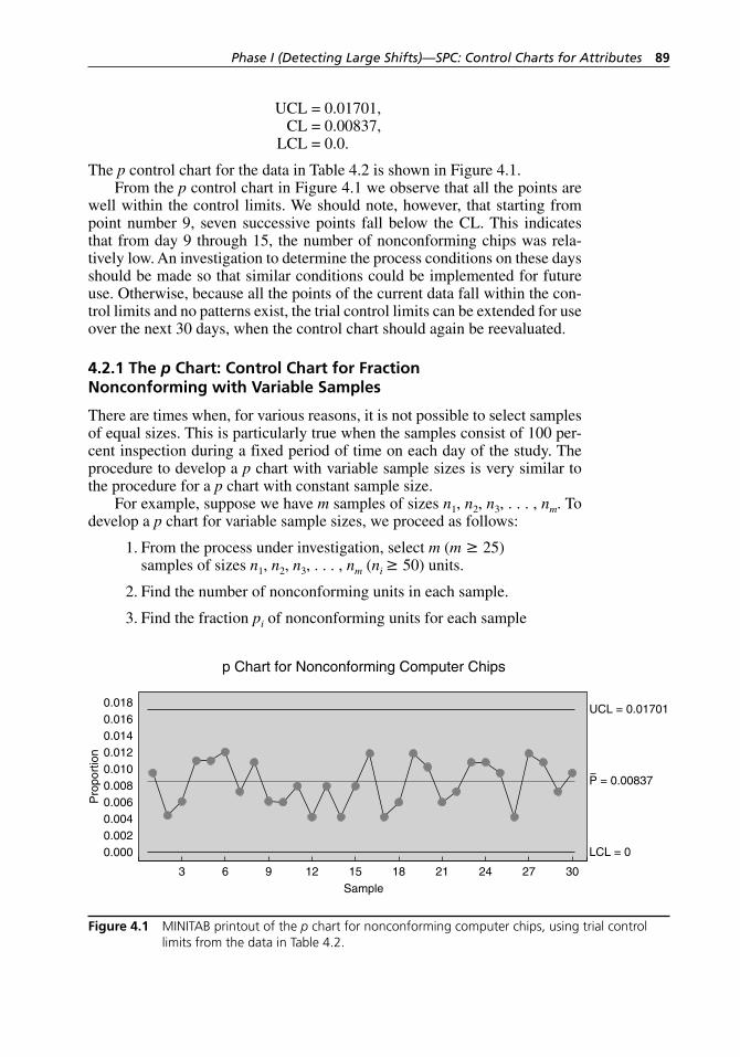
Phase I (Detecting Large Shifts)—SPC: Control Charts for Attributes 89
UCL = 0.01701, CL = 0.00837, LCL = 0.0.
The p control chart for the data in Table 4.2 is shown in Figure 4.1.From the p control chart in Figure 4.1 we observe that all the points are
well within the control limits. We should note, however, that starting from point number 9, seven successive points fall below the CL. This indicates that from day 9 through 15, the number of nonconforming chips was rela-tively low. An investigation to determine the process conditions on these days should be made so that similar conditions could be implemented for future use. Otherwise, because all the points of the current data fall within the con-trol limits and no patterns exist, the trial control limits can be extended for use over the next 30 days, when the control chart should again be reevaluated.
4.2.1 The p Chart: Control Chart for Fraction Nonconforming with Variable Samples
There are times when, for various reasons, it is not possible to select samples of equal sizes. This is particularly true when the samples consist of 100 per-cent inspection during a fixed period of time on each day of the study. The procedure to develop a p chart with variable sample sizes is very similar to the procedure for a p chart with constant sample size.
For example, suppose we have m samples of sizes n1, n2, n3, . . . , nm. To develop a p chart for variable sample sizes, we proceed as follows:
1. From the process under investigation, select m (m ≥ 25) samples of sizes n1, n2, n3, . . . , nm (ni ≥ 50) units.
2. Find the number of nonconforming units in each sample.
3. Find the fraction pi of nonconforming units for each sample
0.0000.0020.0040.0060.0080.0100.0120.0140.0160.018
30272421181512963
UCL = 0.01701
P = 0.00837
LCL = 0
Sample
p Chart for Nonconforming Computer Chips
Pro
port
ion
Figure 4.1 MINITAB printout of the p chart for nonconforming computer chips, using trial control limits from the data in Table 4.2.
H1277 ch04.indd 89H1277 ch04.indd 89 3/8/07 5:50:07 PM3/8/07 5:50:07 PM
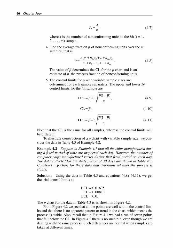
90 Chapter Four
p
x
nii
= ,
(4.7)
where x is the number of nonconforming units in the ith (i = 1, 2, . . . , m) sample.
4. Find the average fraction p– of nonconforming units over the m samples, that is,
p
n p n p n p
n n n nm m
m
=+ + +
+ + + +1 1 2 2
1 2 3
...
....
(4.8)
The value of p– determines the CL for the p chart and is an estimate of p, the process fraction of nonconforming units.
5. The control limits for p with variable sample sizes are determined for each sample separately. The upper and lower 3σ control limits for the ith sample are
UCL = +
−p
p p
ni
31( )
,
(4.9)
CL = p, (4.10)
LCL = −
−p
p p
ni
31( )
.
(4.11)
Note that the CL is the same for all samples, whereas the control limits will be different.
To illustrate construction of a p chart with variable sample size, we con-sider the data in Table 4.3 of Example 4.2.
Example 4.2 Suppose in Example 4.1 that all the chips manufactured dur-ing a fixed period of time are inspected each day. However, the number of computer chips manufactured varies during that fixed period on each day. The data collected for the study period of 30 days are shown in Table 4.3. Construct a p chart for these data and determine whether the process is stable.
Solution: Using the data in Table 4.3 and equations (4.8)–(4.11), we get the trial control limits as
UCL = 0.01675, CL = 0.00813, LCL = 0.0.
The p chart for the data in Table 4.3 is as shown in Figure 4.2.From Figure 4.2 we see that all the points are well within the control lim-
its and that there is no apparent pattern or trend in the chart, which means the process is stable. Also, recall that in Figure 4.1 we had a run of seven points that fell below the CL. In Figure 4.2 there is no such run, even though we are dealing with the same process. Such differences are normal when samples are taken at different times.
H1277 ch04.indd 90H1277 ch04.indd 90 3/8/07 5:50:07 PM3/8/07 5:50:07 PM
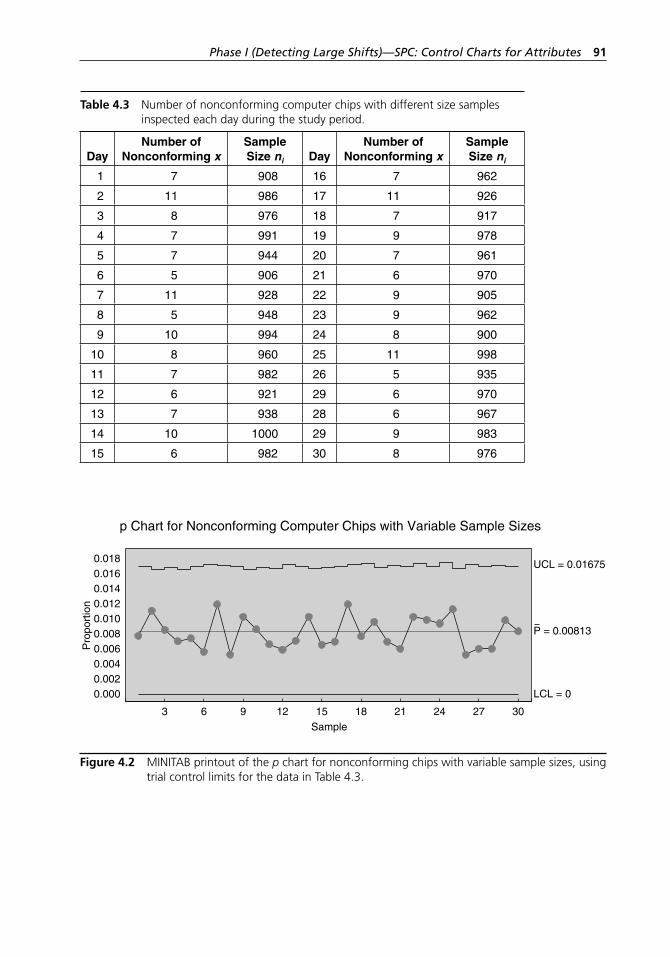
Phase I (Detecting Large Shifts)—SPC: Control Charts for Attributes 91
Table 4.3 Number of nonconforming computer chips with different size samples inspected each day during the study period.
DayNumber of
Nonconforming xSample Size ni Day
Number of Nonconforming x
Sample Size ni
1 7 908 16 7 962
2 11 986 17 11 926
3 8 976 18 7 917
4 7 991 19 9 978
5 7 944 20 7 961
6 5 906 21 6 970
7 11 928 22 9 905
8 5 948 23 9 962
9 10 994 24 8 900
10 8 960 25 11 998
11 7 982 26 5 935
12 6 921 29 6 970
13 7 938 28 6 967
14 10 1000 29 9 983
15 6 982 30 8 976
0.0000.0020.0040.0060.0080.0100.0120.0140.0160.018
30272421181512963
UCL = 0.01675
P = 0.00813
LCL = 0
Sample
p Chart for Nonconforming Computer Chips with Variable Sample Sizes
Pro
port
ion
Figure 4.2 MINITAB printout of the p chart for nonconforming chips with variable sample sizes, using trial control limits for the data in Table 4.3.
H1277 ch04.indd 91H1277 ch04.indd 91 3/8/07 5:50:07 PM3/8/07 5:50:07 PM
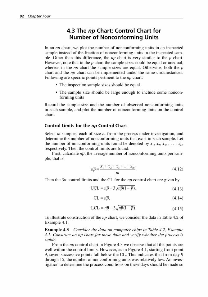
92 Chapter Four
4.3 The np Chart: Control Chart for Number of Nonconforming Units
In an np chart, we plot the number of nonconforming units in an inspected sample instead of the fraction of nonconforming units in the inspected sam-ple. Other than this difference, the np chart is very similar to the p chart. However, note that in the p chart the sample sizes could be equal or unequal, whereas in the np chart the sample sizes are equal. Otherwise, both the p chart and the np chart can be implemented under the same circumstances. Following are specific points pertinent to the np chart:
The inspection sample sizes should be equal
The sample size should be large enough to include some noncon-forming units
Record the sample size and the number of observed nonconforming units in each sample, and plot the number of nonconforming units on the control chart.
Control Limits for the np Control Chart
Select m samples, each of size n, from the process under investigation, and determine the number of nonconforming units that exist in each sample. Let the number of nonconforming units found be denoted by x1, x2, x3, . . . , xm, respectively. Then the control limits are found.
First, calculate np–, the average number of nonconforming units per sam-ple, that is,
np
x x x x
mm=
+ + + +1 2 3 ....
(4.12)
Then the 3σ control limits and the CL for the np control chart are given by
UCL = + −np np p3 1( ),
(4.13)
CL = np, (4.14)
LCL = − −np np p3 1( ).
(4.15)
To illustrate construction of the np chart, we consider the data in Table 4.2 of Example 4.1.
Example 4.3 Consider the data on computer chips in Table 4.2, Example 4.1. Construct an np chart for these data and verify whether the process is stable.
From the np control chart in Figure 4.3 we observe that all the points are well within the control limits. However, as in Figure 4.1, starting from point 9, seven successive points fall below the CL. This indicates that from day 9 through 15, the number of nonconforming units was relatively low. An inves-tigation to determine the process conditions on these days should be made so
•
•
H1277 ch04.indd 92H1277 ch04.indd 92 3/8/07 5:50:07 PM3/8/07 5:50:07 PM
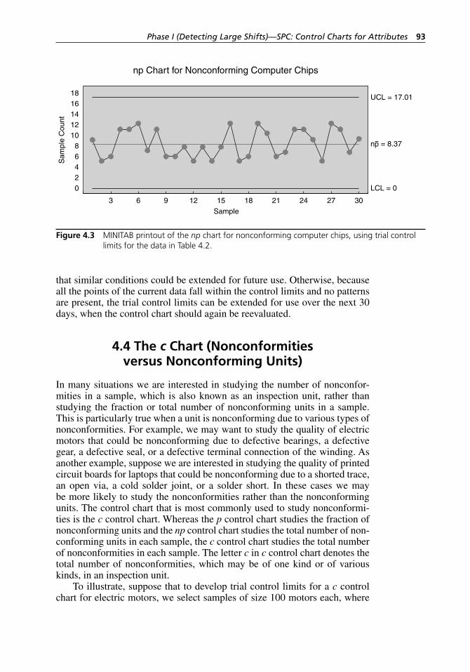
Phase I (Detecting Large Shifts)—SPC: Control Charts for Attributes 93
that similar conditions could be extended for future use. Otherwise, because all the points of the current data fall within the control limits and no patterns are present, the trial control limits can be extended for use over the next 30 days, when the control chart should again be reevaluated.
4.4 The c Chart (Nonconformities versus Nonconforming Units)
In many situations we are interested in studying the number of nonconfor-mities in a sample, which is also known as an inspection unit, rather than studying the fraction or total number of nonconforming units in a sample. This is particularly true when a unit is nonconforming due to various types of nonconformities. For example, we may want to study the quality of electric motors that could be nonconforming due to defective bearings, a defective gear, a defective seal, or a defective terminal connection of the winding. As another example, suppose we are interested in studying the quality of printed circuit boards for laptops that could be nonconforming due to a shorted trace, an open via, a cold solder joint, or a solder short. In these cases we may be more likely to study the nonconformities rather than the nonconforming units. The control chart that is most commonly used to study nonconformi-ties is the c control chart. Whereas the p control chart studies the fraction of nonconforming units and the np control chart studies the total number of non-conforming units in each sample, the c control chart studies the total number of nonconformities in each sample. The letter c in c control chart denotes the total number of nonconformities, which may be of one kind or of various kinds, in an inspection unit.
To illustrate, suppose that to develop trial control limits for a c control chart for electric motors, we select samples of size 100 motors each, where
02468
1012141618
30272421181512963
UCL = 17.01
np = 8.37
LCL = 0
Sample
np Chart for Nonconforming Computer ChipsS
ampl
e C
ount
Figure 4.3 MINITAB printout of the np chart for nonconforming computer chips, using trial control limits for the data in Table 4.2.
H1277 ch04.indd 93H1277 ch04.indd 93 3/8/07 5:50:08 PM3/8/07 5:50:08 PM

94 Chapter Four
each sample would be considered as one inspection unit or several inspec-tion units, depending on how the inspection units are defined. Note that the size of an inspection unit is purely a matter of convenience, but the c control charts are constructed with sample sizes or the number of inspection units in a sample being equal. It can be shown that under certain conditions (condi-tions of a Poisson process, which are briefly discussed in Applied Statistics for the Six Sigma Green Belt), the number of nonconformities c is distributed according to a Poisson probability distribution with parameter λ, where λ is the average number of nonconformities per inspection unit. The Poisson probability distribution is defined as
p x
e
xx
x
( )!
, , , , ,= =− λ λ
0 1 2 3 . . .
(4.16)
where the mean and the variance of the Poisson distribution are given by λ. Now suppose that we select m samples, with each sample being one inspec-tion unit, and let the number of nonconformities in these samples be c1, c2, c3, . . . , cm, respectively. Then the parameter λ, which is usually unknown, is estimated by
ˆ ...
.λ = =+ + + +
cc c c c
mm1 2 3
(4.17)
The 3σ control limits for the c control chart are defined as follows:
UCL = +c c3 , (4.18)
CL = c , (4.19)
LCL = −c c3 . (4.20)
Note that for small values of c– (≤ 5), the Poisson distribution is asymmetric: the value of a Type I error (α) above the UCL and below the LCL is usually not the same. For small values of c– it may be more prudent to use probability control limits rather than the 3σ control limits. The probability control limits can be found by using Poisson distribution tables.
To illustrate construction of a c control chart using 3σ control limits, we consider the data in Table 4.4 of Example 4.4.
Example 4.4 A paper mill has detected that almost 90 percent of rejected paper rolls is due to nonconformities of two types: holes and wrinkles in the paper. The Six Sigma Green Belt team in the mill decides to set up control charts to reduce or eliminate the number of these nonconformities. To set up the control charts, the team collected data by taking random samples of five rolls each day for 30 days and counting the number of nonconformities (holes and wrinkles) in each sample. The data are shown in Table 4.4. Set up a c control chart using these data.
Solution: Using the data in Table 4.4, the estimate of the population param-eter is given by
H1277 ch04.indd 94H1277 ch04.indd 94 3/8/07 5:50:08 PM3/8/07 5:50:08 PM
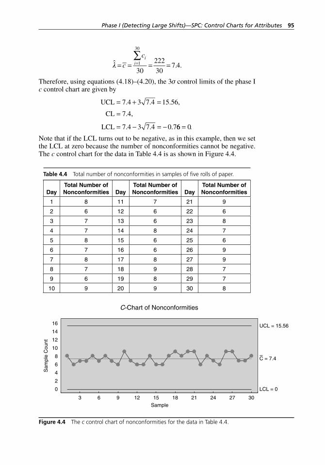
Phase I (Detecting Large Shifts)—SPC: Control Charts for Attributes 95
ˆ . .λ = = = ==
∑c
cii 1
30
30
222
307 4
Therefore, using equations (4.18)–(4.20), the 3σ control limits of the phase I c control chart are given by
UCL
CL
LCL
= + =
=
= − = −
7 4 3 7 4 15 56
7 4
7 4 3 7 4 0 7
. . . ,
. ,
. . . 66 0= .
Note that if the LCL turns out to be negative, as in this example, then we set the LCL at zero because the number of nonconformities cannot be negative. The c control chart for the data in Table 4.4 is as shown in Figure 4.4.
Table 4.4 Total number of nonconformities in samples of five rolls of paper.
DayTotal Number of Nonconformities Day
Total Number of Nonconformities Day
Total Number of Nonconformities
1 8 11 7 21 9
2 6 12 6 22 6
3 7 13 6 23 8
4 7 14 8 24 7
5 8 15 6 25 6
6 7 16 6 26 9
7 8 17 8 27 9
8 7 18 9 28 7
9 6 19 8 29 7
10 9 20 9 30 8
0
2
4
6
8
10
12
14
16
30272421181512963
UCL = 15.56
C = 7.4
LCL = 0
Sample
C-Chart of Nonconformities
Sam
ple
Cou
nt
Figure 4.4 The c control chart of nonconformities for the data in Table 4.4.
H1277 ch04.indd 95H1277 ch04.indd 95 3/8/07 5:50:08 PM3/8/07 5:50:08 PM
96 Chapter Four
From Figure 4.4, we can see that the process is stable. In other words, there are no special causes present, and the only causes that are affecting the process are the common causes. To eliminate the imperfections in the paper, the management must take action on the system, such as examining the qual-ity of the wood chips and pulp, replacing old equipment, and providing more training for the workers. Also, to further enhance the process and eliminate the nonconformities, the quality engineers should use the techniques avail-able in DOE, which we will discuss in our next volume, Design of Experi-ments for the Six Sigma Green Belt.
Notes
1. If the economic factors and time allow, one should take samples or inspection units large enough so that the LCL is positive. The LCL can be positive only if c– > 9. This means that the sample size should be such that it can catch nine or more nonconformities with high probability. An advantage of having a positive LCL is that it will allow us to see the conditions under which the nonconformities are very low, and consequently it will give us the opportunity to perpetuate these conditions on- site and implement them elsewhere in the industry.
2. As noted earlier, the size of the inspection unit is usually determined based on what is convenient. However, to determine the actual inspection unit size, one should also take into consideration the statistical characteristics of the process, such as the ARL, the state of the process (that is, whether the process has deteriorated or improved), and other factors that may require us to increase or decrease the sample size. So, while using control charts for nonconformities, particularly in phase I, situations may arise when the sample size may vary. In these situations, we use the u control chart instead of the c control chart. We will discuss the u control chart in the following section.
If the samples consist of n inspection units, then the control limits for the c control chart are given by
UCL = +nc nc3 , (4.21)
CL = nc , (4.22)
LCL = −nc nc3 . (4.23)
4.5 The u Chart
The u control chart is essentially the c control chart except that the u con-trol chart is always based on the number of nonconformities per inspection
H1277 ch04.indd 96H1277 ch04.indd 96 3/8/07 5:50:08 PM3/8/07 5:50:08 PM
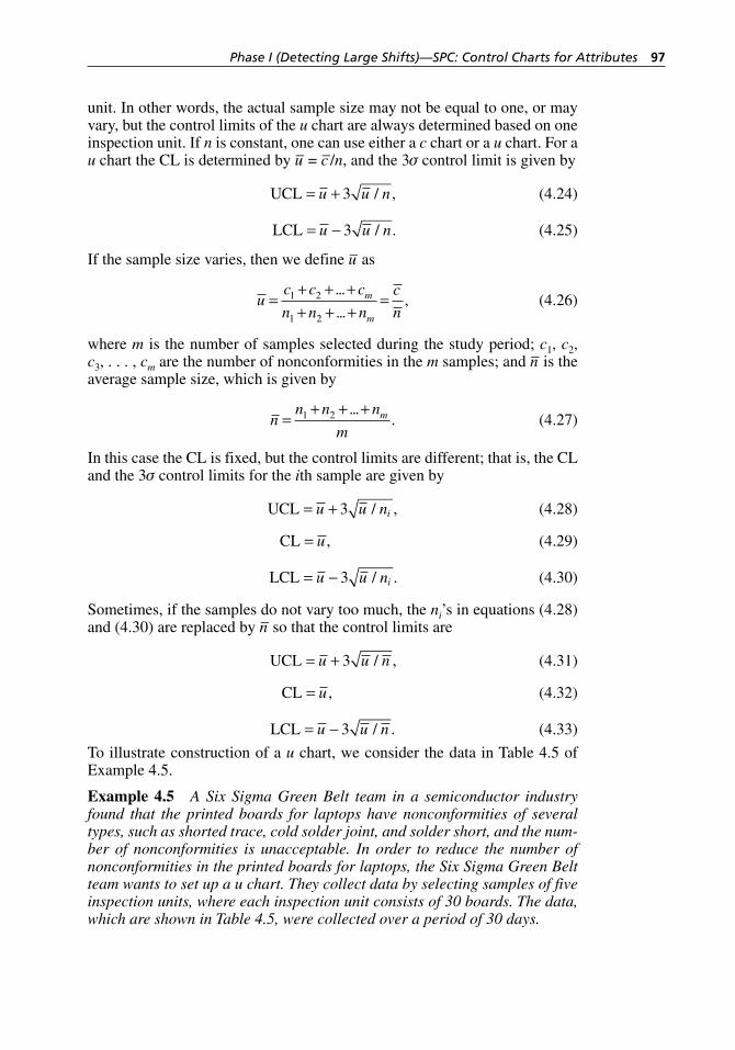
Phase I (Detecting Large Shifts)—SPC: Control Charts for Attributes 97
unit. In other words, the actual sample size may not be equal to one, or may vary, but the control limits of the u chart are always determined based on one inspection unit. If n is constant, one can use either a c chart or a u chart. For a u chart the CL is determined by u– = c–/n, and the 3σ control limit is given by
UCL = +u u n3 / , (4.24)
LCL = −u u n3 / . (4.25)
If the sample size varies, then we define u– as
u
c c c
n n n
c
nm
m
=+ + ++ + +
=1 2
1 2
...
...,
(4.26)
where m is the number of samples selected during the study period; c1, c2, c3, . . . , cm are the number of nonconformities in the m samples; and n– is the average sample size, which is given by
n
n n n
mm=
+ + +1 2 ....
(4.27)
In this case the CL is fixed, but the control limits are different; that is, the CL and the 3σ control limits for the ith sample are given by
UCL = +u u ni3 / , (4.28)
CL = u , (4.29)
LCL = −u u ni3 / . (4.30)
Sometimes, if the samples do not vary too much, the ni’s in equations (4.28) and (4.30) are replaced by n– so that the control limits are
UCL = +u u n3 / , (4.31)
CL = u , (4.32)
LCL = −u u n3 / . (4.33)
To illustrate construction of a u chart, we consider the data in Table 4.5 of Example 4.5.
Example 4.5 A Six Sigma Green Belt team in a semiconductor industry found that the printed boards for laptops have nonconformities of several types, such as shorted trace, cold solder joint, and solder short, and the num-ber of nonconformities is unacceptable. In order to reduce the number of nonconformities in the printed boards for laptops, the Six Sigma Green Belt team wants to set up a u chart. They collect data by selecting samples of five inspection units, where each inspection unit consists of 30 boards. The data, which are shown in Table 4.5, were collected over a period of 30 days.
H1277 ch04.indd 97H1277 ch04.indd 97 3/8/07 5:50:08 PM3/8/07 5:50:08 PM
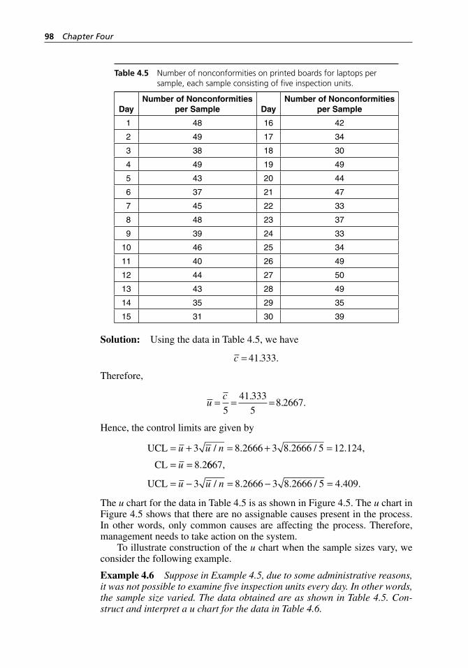
98 Chapter Four
Solution: Using the data in Table 4.5, we have
c = 41 333. .
Therefore,
u
c= = =
5
41 333
58 2667
.. .
Hence, the control limits are given by
UCL
CL
= + = + =
= =
u u n
u
3 8 2666 3 8 2666 5 12 124
8 2
/ . . / . ,
. 6667
3 8 2666 3 8 2666 5 4 409
,
/ . . / . .UCL = − = − =u u n
The u chart for the data in Table 4.5 is as shown in Figure 4.5. The u chart in Figure 4.5 shows that there are no assignable causes present in the process. In other words, only common causes are affecting the process. Therefore, management needs to take action on the system.
To illustrate construction of the u chart when the sample sizes vary, we consider the following example.
Example 4.6 Suppose in Example 4.5, due to some administrative reasons, it was not possible to examine five inspection units every day. In other words, the sample size varied. The data obtained are as shown in Table 4.5. Con-struct and interpret a u chart for the data in Table 4.6.
Table 4.5 Number of nonconformities on printed boards for laptops per sample, each sample consisting of five inspection units.
DayNumber of Nonconformities
per Sample DayNumber of Nonconformities
per Sample
1 48 16 42
2 49 17 34
3 38 18 30
4 49 19 49
5 43 20 44
6 37 21 47
7 45 22 33
8 48 23 37
9 39 24 33
10 46 25 34
11 40 26 49
12 44 27 50
13 43 28 49
14 35 29 35
15 31 30 39
H1277 ch04.indd 98H1277 ch04.indd 98 3/8/07 5:50:09 PM3/8/07 5:50:09 PM
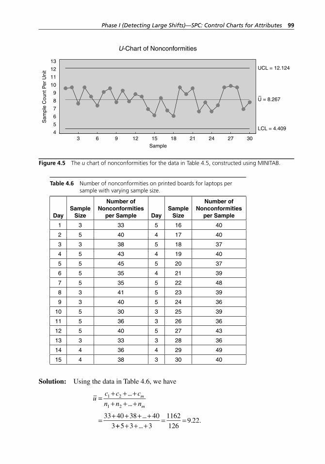
Phase I (Detecting Large Shifts)—SPC: Control Charts for Attributes 99
Solution: Using the data in Table 4.6, we have
uc c c
n n nm
m
=+ + ++ + +
=+ + + +
1 2
1 2
33 40 38 40
3
...
...
...
++ + + += =
5 3 3
1162
1269 22
.... .
5
4
6
7
8
9
10
11
12
13
30272421181512963
UCL = 12.124
U = 8.267
LCL = 4.409
Sample
U-Chart of NonconformitiesS
ampl
e C
ount
Per
Uni
t
Figure 4.5 The u chart of nonconformities for the data in Table 4.5, constructed using MINITAB.
Table 4.6 Number of nonconformities on printed boards for laptops per sample with varying sample size.
DaySample
Size
Number of Nonconformities
per Sample DaySample
Size
Number of Nonconformities
per Sample
1 3 33 5 16 40
2 5 40 4 17 40
3 3 38 5 18 37
4 5 43 4 19 40
5 5 45 5 20 37
6 5 35 4 21 39
7 5 35 5 22 48
8 3 41 5 23 39
9 3 40 5 24 36
10 5 30 3 25 39
11 5 36 3 26 36
12 5 40 5 27 43
13 3 33 3 28 36
14 4 36 4 29 49
15 4 38 3 30 40
H1277 ch04.indd 99H1277 ch04.indd 99 3/8/07 5:50:09 PM3/8/07 5:50:09 PM
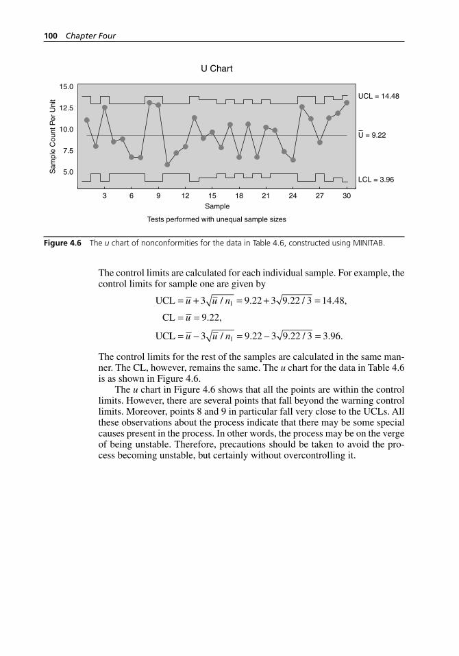
100 Chapter Four
The control limits are calculated for each individual sample. For example, the control limits for sample one are given by
UCL
CL
UC
= + = + =
= =
u u n
u
3 9 22 3 9 22 3 14 48
9 22
1/ . . / . ,
. ,
LL = − = − =u u n3 9 22 3 9 22 3 3 961/ . . / . .
The control limits for the rest of the samples are calculated in the same man-ner. The CL, however, remains the same. The u chart for the data in Table 4.6 is as shown in Figure 4.6.
The u chart in Figure 4.6 shows that all the points are within the control limits. However, there are several points that fall beyond the warning control limits. Moreover, points 8 and 9 in particular fall very close to the UCLs. All these observations about the process indicate that there may be some special causes present in the process. In other words, the process may be on the verge of being unstable. Therefore, precautions should be taken to avoid the pro-cess becoming unstable, but certainly without overcontrolling it.
5.0
7.5
10.0
12.5
15.0
30272421181512963
UCL = 14.48
U = 9.22
LCL = 3.96
Sample
U Chart
Sam
ple
Cou
nt P
er U
nit
Tests performed with unequal sample sizes
Figure 4.6 The u chart of nonconformities for the data in Table 4.6, constructed using MINITAB.
H1277 ch04.indd 100H1277 ch04.indd 100 3/8/07 5:50:09 PM3/8/07 5:50:09 PM
101
In Chapters 3 and 4 we studied Shewhart control charts for detecting large shifts in any process. In this chapter we will study the next generation of control charts: cumulative sum (CUSUM), moving average (MA), and
exponentially weighted moving average (EWMA) control charts. As noted earlier, the large shifts usually occur in phase I of implementing SPC, when a process has a strong influence of special causes and, consequently, large shifts are occurring in the process. By the time phase I implementation of SPC is over, most of the special causes are eliminated or at least reduced, and as a result, the occurrence of large shifts becomes a rare event. In other words, after phase I implementation of SPC is complete and phase II imple-mentation commences, the process is usually under control; as a result, it may be having only small shifts. Shewhart control charts are known to be not very effective in detecting small shifts that are less than 1.5σ. One possibility when the shifts are small is to increase the sensitivity of the Shewhart control charts by using the following criteria from Western Electric (1956, 27):
a. Two out of three consecutive points fall outside the 2σ warning limits
b. Four out of five consecutive points fall at a distance of 1σ or more from the CL
c. Eight consecutive points fall above or below the CL
5
Phase II (Detecting Small Shifts)—SPC: Cumulative Sum, Moving Average,
and Exponentially Weighted Moving
Average Control Charts
H1277 ch05.indd 101H1277 ch05.indd 101 3/8/07 12:35:02 PM3/8/07 12:35:02 PM
102 Chapter Five
If one point falls outside the 3σ control limits or if any conditions from this list occur, the process is considered to be out of control. Subsequently, an appropriate action is taken, such as increasing the sampling frequency, increasing the sample size, or both. However, even though these actions do increase the sensitivity, as Champ and Woodall (1987) point out, using these rules, the in- control ARL is only 91.75. Under normality, the false- alarm rate is little more than four times the false- alarm rate of a Shewhart chart when the criteria from Western Electric are not used. Moreover, the advantage of the simplicity of Shewhart charts, which is an important feature, is lost. Keeping all this in mind, it is fair to say that when the shifts are small, the Shewhart chart with these modifications is not a viable alternative to the CUSUM con-trol chart. Also, the CUSUM control chart has another major advantage over the Shewhart control chart. In the CUSUM control chart, the ith point uses the information contained in all the samples collected at time i and before, whereas the Shewhart control chart uses only the information contained in the ith sample. In other words, the Shewhart control chart ignores all infor-mation provided by the samples collected before the ith sample. But at the same time, we must note that this feature of the CUSUM control chart makes the plotted points dependent, and therefore it is difficult to interpret any pat-tern other than when the point exceeds the decision interval for an upward or downward shift.
Other control charts that are very effective in detecting small shifts are the MA and EWMA control charts. CUSUM, MA, and EWMA control charts are excellent alternatives to the Shewhart control chart for controlling processes in phase II. Relatively speaking, the MA chart is not as effective as CUSUM and EWMA charts. The CUSUM and EWMA control charts can be used to monitor not only the process mean but also the process variance and the fraction nonconforming and nonconformities. However, our major focus of discussion of these control charts is on the process mean. An excel-lent reference for a detailed study of CUSUM control charts is Hawkins and Olwell (1998).
5.1 Basic Concepts of the CUSUM Control Chart
CUSUM Control Chart versus Shewhart X–-R Control Chart
The basic assumptions of a CUSUM control chart are:
1. The observations are independently and identically normally distributed with mean µ and standard deviation σ.
2. The mean µ and standard deviation σ are known.
Note that in practice the parameters µ and σ are never known. Hence, we always end up estimating them. It is very important to remember that while estimating these parameters, precision is essential. Even a small error, par-ticularly in estimating µ, will have an accumulative effect, which will cause false alarms. One way to avoid such problems is to take very large samples when estimating these parameters.
H1277 ch05.indd 102H1277 ch05.indd 102 3/8/07 12:35:03 PM3/8/07 12:35:03 PM
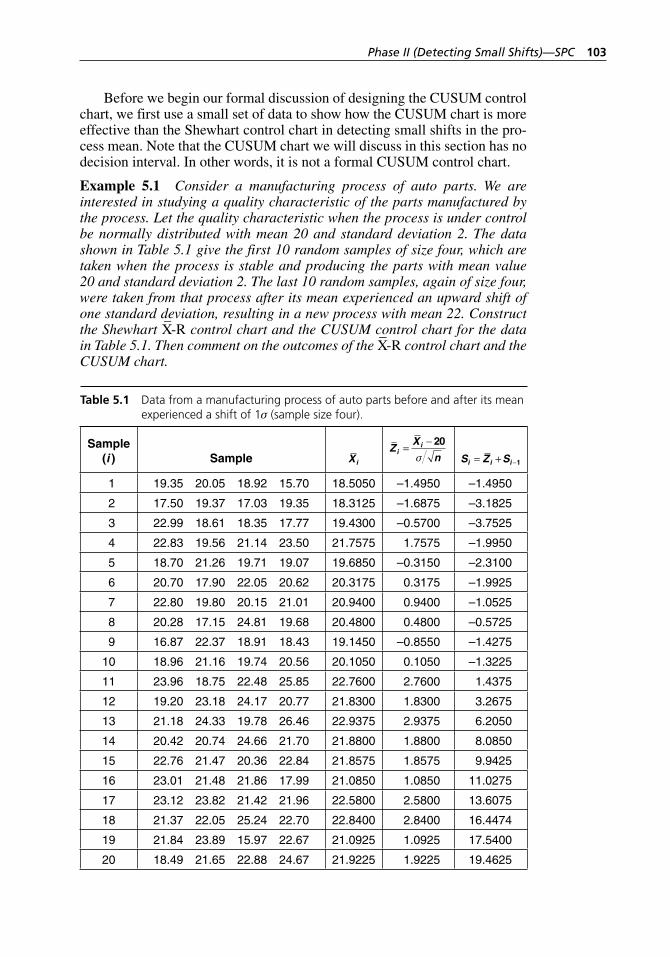
Phase II (Detecting Small Shifts)—SPC 103
Before we begin our formal discussion of designing the CUSUM control chart, we first use a small set of data to show how the CUSUM chart is more effective than the Shewhart control chart in detecting small shifts in the pro-cess mean. Note that the CUSUM chart we will discuss in this section has no decision interval. In other words, it is not a formal CUSUM control chart.
Example 5.1 Consider a manufacturing process of auto parts. We are interested in studying a quality characteristic of the parts manufactured by the process. Let the quality characteristic when the process is under control be normally distributed with mean 20 and standard deviation 2. The data shown in Table 5.1 give the first 10 random samples of size four, which are taken when the process is stable and producing the parts with mean value 20 and standard deviation 2. The last 10 random samples, again of size four, were taken from that process after its mean experienced an upward shift of one standard deviation, resulting in a new process with mean 22. Construct the Shewhart X
–-R control chart and the CUSUM control chart for the data
in Table 5.1. Then comment on the outcomes of the X–-R control chart and the
CUSUM chart.
Table 5.1 Data from a manufacturing process of auto parts before and after its mean experienced a shift of 1σ (sample size four).
Sample (i ) Sample Xi
ZX
ni
i= − 20
σ S Z Si i i= + −1
1 19.35 20.05 18.92 15.70 18.5050 –1.4950 –1.4950
2 17.50 19.37 17.03 19.35 18.3125 –1.6875 –3.1825
3 22.99 18.61 18.35 17.77 19.4300 –0.5700 –3.7525
4 22.83 19.56 21.14 23.50 21.7575 1.7575 –1.9950
5 18.70 21.26 19.71 19.07 19.6850 –0.3150 –2.3100
6 20.70 17.90 22.05 20.62 20.3175 0.3175 –1.9925
7 22.80 19.80 20.15 21.01 20.9400 0.9400 –1.0525
8 20.28 17.15 24.81 19.68 20.4800 0.4800 –0.5725
9 16.87 22.37 18.91 18.43 19.1450 –0.8550 –1.4275
10 18.96 21.16 19.74 20.56 20.1050 0.1050 –1.3225
11 23.96 18.75 22.48 25.85 22.7600 2.7600 1.4375
12 19.20 23.18 24.17 20.77 21.8300 1.8300 3.2675
13 21.18 24.33 19.78 26.46 22.9375 2.9375 6.2050
14 20.42 20.74 24.66 21.70 21.8800 1.8800 8.0850
15 22.76 21.47 20.36 22.84 21.8575 1.8575 9.9425
16 23.01 21.48 21.86 17.99 21.0850 1.0850 11.0275
17 23.12 23.82 21.42 21.96 22.5800 2.5800 13.6075
18 21.37 22.05 25.24 22.70 22.8400 2.8400 16.4474
19 21.84 23.89 15.97 22.67 21.0925 1.0925 17.5400
20 18.49 21.65 22.88 24.67 21.9225 1.9225 19.4625
H1277 ch05.indd 103H1277 ch05.indd 103 3/8/07 12:35:03 PM3/8/07 12:35:03 PM
104 Chapter Five
Solution: As described earlier, the basic principle of the CUSUM chart is to detect small shifts in the process mean at time i by calculating the accumu-lated sum Si of deviations of the sample means X X Xi1 2, , . . . , from the target value (µ0) measured in standard deviation units. That is,
SX
n
X
nS
Z S
ij
j
ii
i
i i
=−
=−
+
= +=
−
−
∑( ) ( )
,
µ
σ
µ
σ
0
1
01
1
(5.1)
where Z Z Zi1 2, , . . . , are the standardized values of X X Xi1 2, , . . . , , respec-tively. In Example 5.1, the target value is 20 and the accumulated sum of deviations of the sample means from the target value at time i, when mea-sured in standard deviation units, is given in column 5 of Table 5.1. From equation (5.1) one can see that if the samples come from a stable process with mean µ1, the points (i, Si) when plotted on a chart will:
a. Randomly scatter around the zero line
b. Clearly show an upward trend
c. Clearly show a downward trend
The result depends on whether µ1 = µ0, µ1 > µ0, or µ1 < µ0.The X
–-R control chart and the CUSUM chart are as shown in Figures 5.1
and 5.2. The X–-R control chart shows that the process is clearly stable and
showing no abnormality other than sample number 13, which comes close to the UCL. In other words, the chart is not detecting that the samples start-ing with the 11th sample came from the process after it had experienced an upward shift of one standard deviation. However, the CUSUM chart shows an upward trend, which started at the 11th sample. Furthermore, as noted by Lucas (1982), CUSUM control charts give tighter process control than clas-sical control charts such as Shewhart control charts. With the tighter control provided by CUSUM control charts, more emphasis is placed on keeping the process on target rather than allowing it to drift within the limits. Moreover, the sensitivity of the CUSUM control chart would not be seriously affected if we took samples of size n = 1 instead of n > 1. In fact, CUSUM control charts more frequently use n = 1 or individual values. In CUSUM control charts for individual values, the quantities X
–i, Z
–i, and σ/ n in Table 5.1 are replaced by
Xi, Zi, and σ, respectively. We will look at developing the CUSUM control chart in the next section.
5.2 Designing a CUSUM Control Chart
In section 5.1 we saw that CUSUM charts are very effective in detecting small shifts. Unlike the X
– Shewhart control charts, CUSUM control charts
can be designed to detect one- sided or two- sided shifts. These charts are defined by two parameters, k and h, called the reference value and the deci-sion interval, which are defined in section 5.2.1. The two- sided process con-trol using the CUSUM control chart is achieved by concurrently using two
H1277 ch05.indd 104H1277 ch05.indd 104 3/8/07 12:35:03 PM3/8/07 12:35:03 PM
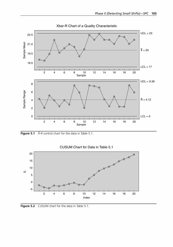
Phase II (Detecting Small Shifts)—SPC 105
18.0
19.5
21.0
22.5
2018161412108642
UCL = 23
X = 20
LCL = 17
Sample
Xbar-R Chart of a Quality CharacteristicS
ampl
e M
ean
0
2
4
6
8
2018161412108642
UCL = 9.39
R = 4.12
LCL = 0
Sample
Sam
ple
Ran
ge
Figure 5.1 X–-R control chart for the data in Table 5.1.
5
0
-5
10
15
20
2018161412108642Index
iS
CUSUM Chart for Data in Table 5.1
Figure 5.2 CUSUM chart for the data in Table 5.1.
H1277 ch05.indd 105H1277 ch05.indd 105 3/8/07 12:35:03 PM3/8/07 12:35:03 PM
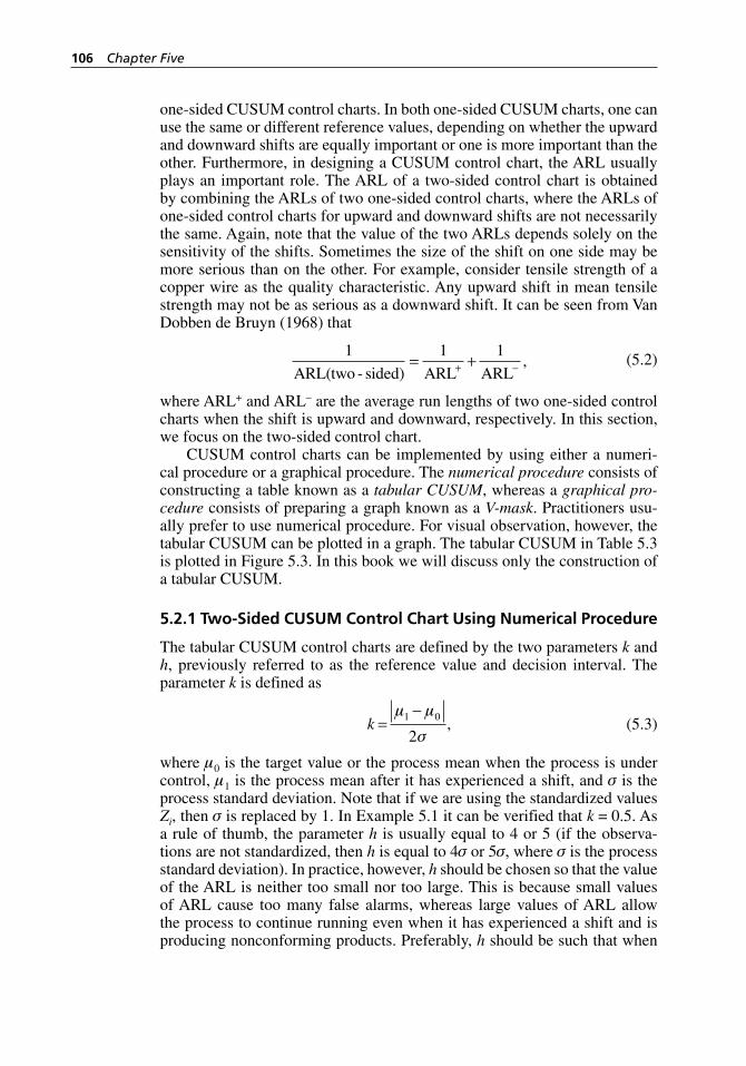
106 Chapter Five
one- sided CUSUM control charts. In both one- sided CUSUM charts, one can use the same or different reference values, depending on whether the upward and downward shifts are equally important or one is more important than the other. Furthermore, in designing a CUSUM control chart, the ARL usually plays an important role. The ARL of a two- sided control chart is obtained by combining the ARLs of two one- sided control charts, where the ARLs of one- sided control charts for upward and downward shifts are not necessarily the same. Again, note that the value of the two ARLs depends solely on the sensitivity of the shifts. Sometimes the size of the shift on one side may be more serious than on the other. For example, consider tensile strength of a copper wire as the quality characteristic. Any upward shift in mean tensile strength may not be as serious as a downward shift. It can be seen from Van Dobben de Bruyn (1968) that
1 1 1
ARL(two - sided) ARL ARL= ++ − ,
(5.2)
where ARL+ and ARL– are the average run lengths of two one- sided control charts when the shift is upward and downward, respectively. In this section, we focus on the two- sided control chart.
CUSUM control charts can be implemented by using either a numeri-cal procedure or a graphical procedure. The numerical procedure consists of constructing a table known as a tabular CUSUM, whereas a graphical pro-cedure consists of preparing a graph known as a V-mask. Practitioners usu-ally prefer to use numerical procedure. For visual observation, however, the tabular CUSUM can be plotted in a graph. The tabular CUSUM in Table 5.3 is plotted in Figure 5.3. In this book we will discuss only the construction of a tabular CUSUM.
5.2.1 Two- Sided CUSUM Control Chart Using Numerical Procedure
The tabular CUSUM control charts are defined by the two parameters k and h, previously referred to as the reference value and decision interval. The parameter k is defined as
k =
−µ µ
σ1 0
2,
(5.3)
where µ0 is the target value or the process mean when the process is under control, µ1 is the process mean after it has experienced a shift, and σ is the process standard deviation. Note that if we are using the standardized values Zi, then σ is replaced by 1. In Example 5.1 it can be verified that k = 0.5. As a rule of thumb, the parameter h is usually equal to 4 or 5 (if the observa-tions are not standardized, then h is equal to 4σ or 5σ, where σ is the process standard deviation). In practice, however, h should be chosen so that the value of the ARL is neither too small nor too large. This is because small values of ARL cause too many false alarms, whereas large values of ARL allow the process to continue running even when it has experienced a shift and is producing nonconforming products. Preferably, h should be such that when
H1277 ch05.indd 106H1277 ch05.indd 106 3/8/07 12:35:04 PM3/8/07 12:35:04 PM
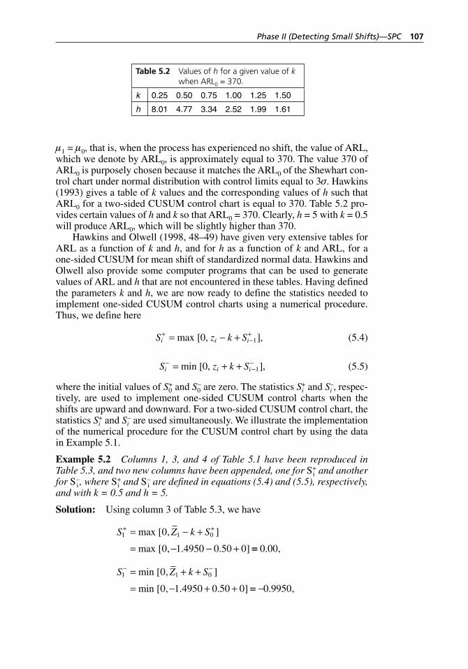
Phase II (Detecting Small Shifts)—SPC 107
µ1 = µ0, that is, when the process has experienced no shift, the value of ARL, which we denote by ARL0, is approximately equal to 370. The value 370 of ARL0 is purposely chosen because it matches the ARL0 of the Shewhart con-trol chart under normal distribution with control limits equal to 3σ. Hawkins (1993) gives a table of k values and the corresponding values of h such that ARL0 for a two-sided CUSUM control chart is equal to 370. Table 5.2 pro-vides certain values of h and k so that ARL0 = 370. Clearly, h = 5 with k = 0.5 will produce ARL0, which will be slightly higher than 370.
Hawkins and Olwell (1998, 48–49) have given very extensive tables for ARL as a function of k and h, and for h as a function of k and ARL, for a one- sided CUSUM for mean shift of standardized normal data. Hawkins and Olwell also provide some computer programs that can be used to generate values of ARL and h that are not encountered in these tables. Having defined the parameters k and h, we are now ready to define the statistics needed to implement one- sided CUSUM control charts using a numerical procedure. Thus, we define here
S z k Si i i+
−+= − +max [0, 1], (5.4)
S z k Si i i−
−−= + +min [0, 1], (5.5)
where the initial values of S0+ and S0
– are zero. The statistics Si+ and Si
–, respec-tively, are used to implement one- sided CUSUM control charts when the shifts are upward and downward. For a two- sided CUSUM control chart, the statistics Si
+ and Si– are used simultaneously. We illustrate the implementation
of the numerical procedure for the CUSUM control chart by using the data in Example 5.1.
Example 5.2 Columns 1, 3, and 4 of Table 5.1 have been reproduced in Table 5.3, and two new columns have been appended, one for Si
+ and another for Si
–, where Si+ and Si
– are defined in equations (5.4) and (5.5), respectively, and with k = 0.5 and h = 5.
Solution: Using column 3 of Table 5.3, we have
S Z k S1 1 00
0 1 4950 0 50 0
+ += − +
= − − +
max
max
[ , ]
[ , . . ] == 0 00. ,
S Z k S1 1 00
0 1 4950 0 50 0
− −= + +
= − + +
min
min
[ , ]
[ , . . ] == −0 9950. ,
Table 5.2 Values of h for a given value of k when ARL0 = 370.
k 0.25 0.50 0.75 1.00 1.25 1.50
h 8.01 4.77 3.34 2.52 1.99 1.61
H1277 ch05.indd 107H1277 ch05.indd 107 3/8/07 12:35:04 PM3/8/07 12:35:04 PM
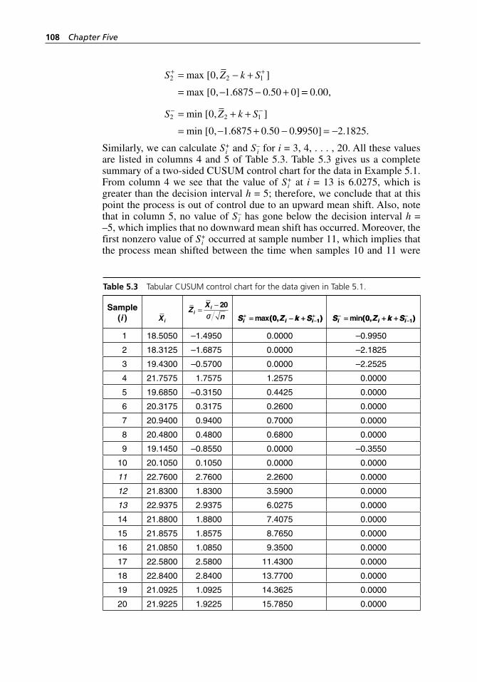
108 Chapter Five
S Z k S2 2 10
0 1 6875 0 50 0
+ += − +
= − − +
max
max
[ , ]
[ , . . ] == 0 00. ,
S Z k S2 2 10
0 1 6875 0 50 0
− −= + +
= − + −
min
min
[ , ]
[ , . . .99950 2 1825] . .= −Similarly, we can calculate Si
+ and S i– for i = 3, 4, . . . , 20. All these values
are listed in columns 4 and 5 of Table 5.3. Table 5.3 gives us a complete summary of a two- sided CUSUM control chart for the data in Example 5.1. From column 4 we see that the value of Si
+ at i = 13 is 6.0275, which is greater than the decision interval h = 5; therefore, we conclude that at this point the process is out of control due to an upward mean shift. Also, note that in column 5, no value of S i
– has gone below the decision interval h = –5, which implies that no downward mean shift has occurred. Moreover, the first nonzero value of Si
+ occurred at sample number 11, which implies that the process mean shifted between the time when samples 10 and 11 were
Table 5.3 Tabular CUSUM control chart for the data given in Table 5.1.
Sample (i ) Xi
ZX
ni
i 20
SS ZZ kk SSii ii ii++
−−++== −− ++max(( ,, ))00 11 SS ZZ kk SSii ii ii
−−−−
−−== ++ ++min(( ,, ))00 11
1 18.5050 –1.4950 0.0000 –0.9950
2 18.3125 –1.6875 0.0000 –2.1825
3 19.4300 –0.5700 0.0000 –2.2525
4 21.7575 1.7575 1.2575 0.0000
5 19.6850 –0.3150 0.4425 0.0000
6 20.3175 0.3175 0.2600 0.0000
7 20.9400 0.9400 0.7000 0.0000
8 20.4800 0.4800 0.6800 0.0000
9 19.1450 –0.8550 0.0000 –0.3550
10 20.1050 0.1050 0.0000 0.0000
11 22.7600 2.7600 2.2600 0.0000
12 21.8300 1.8300 3.5900 0.0000
13 22.9375 2.9375 6.0275 0.0000
14 21.8800 1.8800 7.4075 0.0000
15 21.8575 1.8575 8.7650 0.0000
16 21.0850 1.0850 9.3500 0.0000
17 22.5800 2.5800 11.4300 0.0000
18 22.8400 2.8400 13.7700 0.0000
19 21.0925 1.0925 14.3625 0.0000
20 21.9225 1.9225 15.7850 0.0000
H1277 ch05.indd 108H1277 ch05.indd 108 3/8/07 12:35:05 PM3/8/07 12:35:05 PM
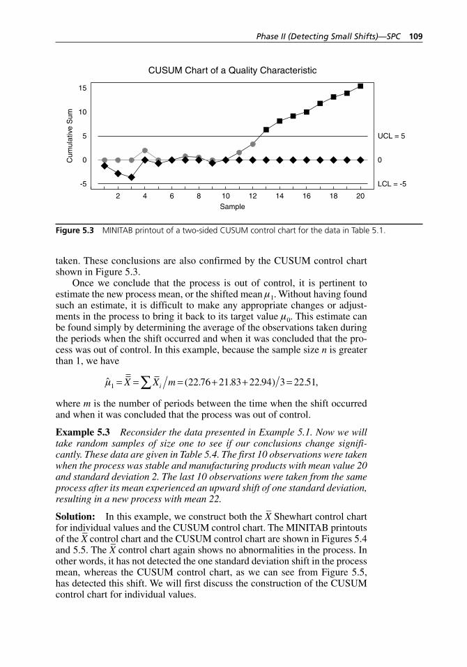
Phase II (Detecting Small Shifts)—SPC 109
taken. These conclusions are also confirmed by the CUSUM control chart shown in Figure 5.3.
Once we conclude that the process is out of control, it is pertinent to estimate the new process mean, or the shifted mean µ1. Without having found such an estimate, it is difficult to make any appropriate changes or adjust-ments in the process to bring it back to its target value µ0. This estimate can be found simply by determining the average of the observations taken during the periods when the shift occurred and when it was concluded that the pro-cess was out of control. In this example, because the sample size n is greater than 1, we have
ˆ ( . . . ) . ,µ1 22 76 21 83 22 94 3 22 51= = = + + =∑X X mi
where m is the number of periods between the time when the shift occurred and when it was concluded that the process was out of control.
Example 5.3 Reconsider the data presented in Example 5.1. Now we will take random samples of size one to see if our conclusions change signifi-cantly. These data are given in Table 5.4. The first 10 observations were taken when the process was stable and manufacturing products with mean value 20 and standard deviation 2. The last 10 observations were taken from the same process after its mean experienced an upward shift of one standard deviation, resulting in a new process with mean 22.
Solution: In this example, we construct both the X– Shewhart control chart
for individual values and the CUSUM control chart. The MINITAB printouts of the X
– control chart and the CUSUM control chart are shown in Figures 5.4
and 5.5. The X– control chart again shows no abnormalities in the process. In
other words, it has not detected the one standard deviation shift in the process mean, whereas the CUSUM control chart, as we can see from Figure 5.5, has detected this shift. We will first discuss the construction of the CUSUM control chart for individual values.
5
0
-5
10
15
2018161412108642Sample
Cum
ulat
ive
Sum
CUSUM Chart of a Quality Characteristic
UCL = 5
0
LCL = -5
Figure 5.3 MINITAB printout of a two- sided CUSUM control chart for the data in Table 5.1.
H1277 ch05.indd 109H1277 ch05.indd 109 3/8/07 12:35:05 PM3/8/07 12:35:05 PM
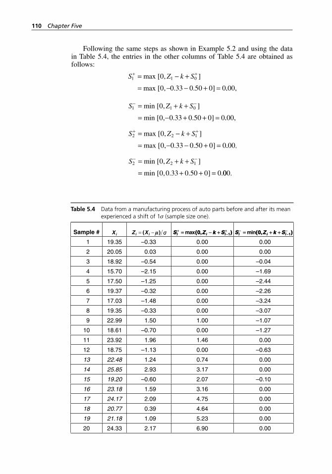
110 Chapter Five
Following the same steps as shown in Example 5.2 and using the data in Table 5.4, the entries in the other columns of Table 5.4 are obtained as follows:
S Z k S1 1 00
0 0 33 0 50 0 0
+ += − +
= − − + =
max
max
[ , ]
[ , . . ] .. ,00
S Z k S1 1 00
0 0 33 0 50 0 0
− −= + +
= − + + =
min
min
[ , ]
[ , . . ] .. ,00
S Z k S2 2 10
0 0 33 0 50 0 0
+ += − +
= − − + =
max
max
[ , ]
[ , . . ] .. ,00
S Z k S2 2 10
0 0 33 0 50 0 0
− −= + +
= + + =
min
min
[ , ]
[ , . . ] .000.
Table 5.4 Data from a manufacturing process of auto parts before and after its mean experienced a shift of 1σ (sample size one).
Sample # Xi Z Xi i( ) SS ZZ kk SSii ii ii++
−−++== −− ++max(( ,, ))00 11 SS ZZ kk SSii ii ii
−−−−
−−== ++ ++min(( ,, ))00 11
1 19.35 –0.33 0.00 0.00
2 20.05 0.03 0.00 0.00
3 18.92 –0.54 0.00 –0.04
4 15.70 –2.15 0.00 –1.69
5 17.50 –1.25 0.00 –2.44
6 19.37 –0.32 0.00 –2.26
7 17.03 –1.48 0.00 –3.24
8 19.35 –0.33 0.00 –3.07
9 22.99 1.50 1.00 –1.07
10 18.61 –0.70 0.00 –1.27
11 23.92 1.96 1.46 0.00
12 18.75 –1.13 0.00 –0.63
13 22.48 1.24 0.74 0.00
14 25.85 2.93 3.17 0.00
15 19.20 –0.60 2.07 –0.10
16 23.18 1.59 3.16 0.00
17 24.17 2.09 4.75 0.00
18 20.77 0.39 4.64 0.00
19 21.18 1.09 5.23 0.00
20 24.33 2.17 6.90 0.00
H1277 ch05.indd 110H1277 ch05.indd 110 3/8/07 12:35:05 PM3/8/07 12:35:05 PM
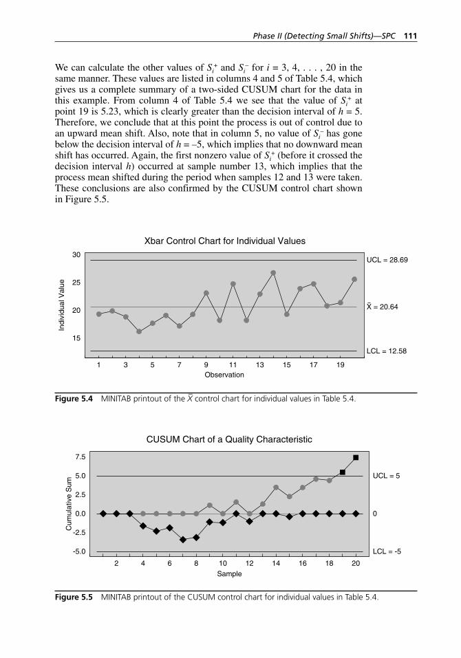
Phase II (Detecting Small Shifts)—SPC 111
We can calculate the other values of Si+ and Si
– for i = 3, 4, . . . , 20 in the same manner. These values are listed in columns 4 and 5 of Table 5.4, which gives us a complete summary of a two- sided CUSUM chart for the data in this example. From column 4 of Table 5.4 we see that the value of Si
+ at point 19 is 5.23, which is clearly greater than the decision interval of h = 5. Therefore, we conclude that at this point the process is out of control due to an upward mean shift. Also, note that in column 5, no value of Si
– has gone below the decision interval of h = –5, which implies that no downward mean shift has occurred. Again, the first nonzero value of Si
+ (before it crossed the decision interval h) occurred at sample number 13, which implies that the process mean shifted during the period when samples 12 and 13 were taken. These conclusions are also confirmed by the CUSUM control chart shown in Figure 5.5.
15
20
25
30
191715131197531
UCL = 28.69
X = 20.64
LCL = 12.58
Observation
Xbar Control Chart for Individual Values
Indi
vidu
al V
alue
Figure 5.4 MINITAB printout of the X– control chart for individual values in Table 5.4.
2.5
0.0
-5.0
-2.5
5.0
7.5
2018161412108642Sample
Cum
ulat
ive
Sum
CUSUM Chart of a Quality Characteristic
UCL = 5
0
LCL = -5
Figure 5.5 MINITAB printout of the CUSUM control chart for individual values in Table 5.4.
H1277 ch05.indd 111H1277 ch05.indd 111 3/8/07 12:35:06 PM3/8/07 12:35:06 PM
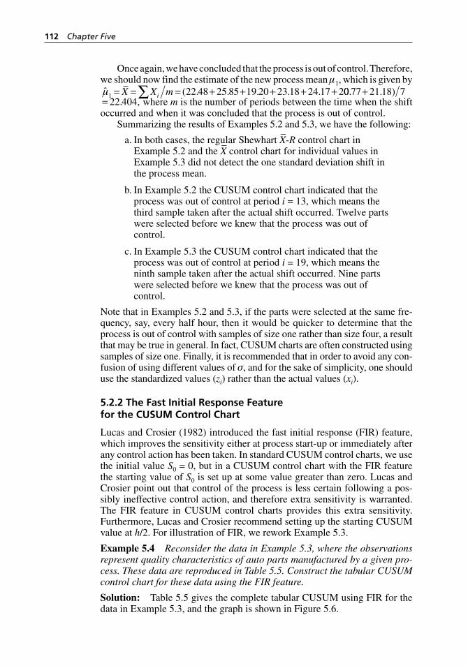
112 Chapter Five
Once again, we have concluded that the process is out of control. Therefore, we should now find the estimate of the new process mean µ1, which is given by ˆ ( . . . . .µ1 22 48 25 85 19 20 23 18 24 17 2= = = + + + + +∑X X mi 00 77 21 18 7. . )+
22 404. ,= where m is the number of periods between the time when the shift occurred and when it was concluded that the process is out of control.
Summarizing the results of Examples 5.2 and 5.3, we have the following:
a. In both cases, the regular Shewhart X–-R control chart in
Example 5.2 and the X– control chart for individual values in
Example 5.3 did not detect the one standard deviation shift in the process mean.
b. In Example 5.2 the CUSUM control chart indicated that the process was out of control at period i = 13, which means the third sample taken after the actual shift occurred. Twelve parts were selected before we knew that the process was out of control.
c. In Example 5.3 the CUSUM control chart indicated that the process was out of control at period i = 19, which means the ninth sample taken after the actual shift occurred. Nine parts were selected before we knew that the process was out of control.
Note that in Examples 5.2 and 5.3, if the parts were selected at the same fre-quency, say, every half hour, then it would be quicker to determine that the process is out of control with samples of size one rather than size four, a result that may be true in general. In fact, CUSUM charts are often constructed using samples of size one. Finally, it is recommended that in order to avoid any con-fusion of using different values of σ, and for the sake of simplicity, one should use the standardized values (zi) rather than the actual values (xi).
5.2.2 The Fast Initial Response Feature for the CUSUM Control Chart
Lucas and Crosier (1982) introduced the fast initial response (FIR) feature, which improves the sensitivity either at process start- up or immediately after any control action has been taken. In standard CUSUM control charts, we use the initial value S0 = 0, but in a CUSUM control chart with the FIR feature the starting value of S0 is set up at some value greater than zero. Lucas and Crosier point out that control of the process is less certain following a pos-sibly ineffective control action, and therefore extra sensitivity is warranted. The FIR feature in CUSUM control charts provides this extra sensitivity. Furthermore, Lucas and Crosier recommend setting up the starting CUSUM value at h/2. For illustration of FIR, we rework Example 5.3.
Example 5.4 Reconsider the data in Example 5.3, where the observations represent quality characteristics of auto parts manufactured by a given pro-cess. These data are reproduced in Table 5.5. Construct the tabular CUSUM control chart for these data using the FIR feature.
Solution: Table 5.5 gives the complete tabular CUSUM using FIR for the data in Example 5.3, and the graph is shown in Figure 5.6.
H1277 ch05.indd 112H1277 ch05.indd 112 3/8/07 12:35:06 PM3/8/07 12:35:06 PM
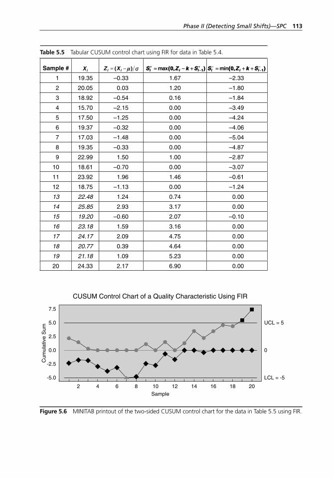
Phase II (Detecting Small Shifts)—SPC 113
Table 5.5 Tabular CUSUM control chart using FIR for data in Table 5.4.
Sample # Xi Z Xi i( ) SS ZZ kk SSii ii ii++
−−++== −− ++max(( ,, ))00 11 SS ZZ kk SSii ii ii
−−−−
−−== ++ ++min(( ,, ))00 11
1 19.35 –0.33 1.67 –2.33
2 20.05 0.03 1.20 –1.80
3 18.92 –0.54 0.16 –1.84
4 15.70 –2.15 0.00 –3.49
5 17.50 –1.25 0.00 –4.24
6 19.37 –0.32 0.00 –4.06
7 17.03 –1.48 0.00 –5.04
8 19.35 –0.33 0.00 –4.87
9 22.99 1.50 1.00 –2.87
10 18.61 –0.70 0.00 –3.07
11 23.92 1.96 1.46 –0.61
12 18.75 –1.13 0.00 –1.24
13 22.48 1.24 0.74 0.00
14 25.85 2.93 3.17 0.00
15 19.20 –0.60 2.07 –0.10
16 23.18 1.59 3.16 0.00
17 24.17 2.09 4.75 0.00
18 20.77 0.39 4.64 0.00
19 21.18 1.09 5.23 0.00
20 24.33 2.17 6.90 0.00
2.5
0.0
-5.0
-2.5
5.0
7.5
2018161412108642Sample
Cum
ulat
ive
Sum
CUSUM Control Chart of a Quality Characteristic Using FIR
UCL = 5
0
LCL = -5
Figure 5.6 MINITAB printout of the two- sided CUSUM control chart for the data in Table 5.5 using FIR.
H1277 ch05.indd 113H1277 ch05.indd 113 3/8/07 12:35:06 PM3/8/07 12:35:06 PM
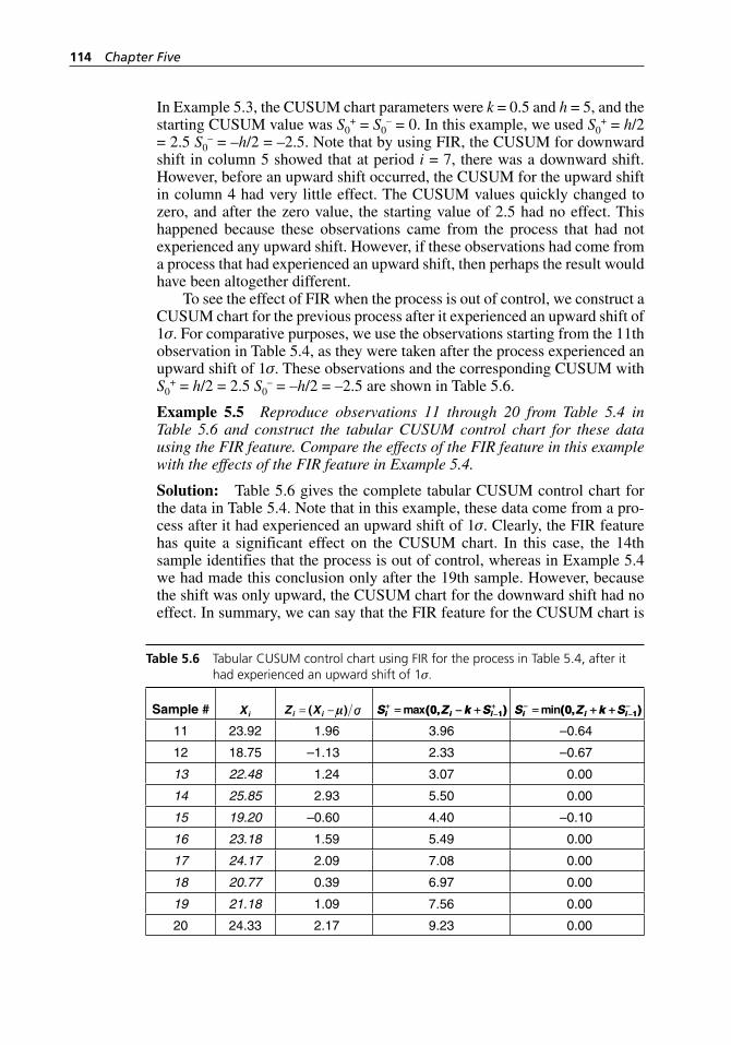
114 Chapter Five
In Example 5.3, the CUSUM chart parameters were k = 0.5 and h = 5, and the starting CUSUM value was S0
+ = S0– = 0. In this example, we used S0
+ = h/2 = 2.5 S0
– = –h/2 = –2.5. Note that by using FIR, the CUSUM for downward shift in column 5 showed that at period i = 7, there was a downward shift. However, before an upward shift occurred, the CUSUM for the upward shift in column 4 had very little effect. The CUSUM values quickly changed to zero, and after the zero value, the starting value of 2.5 had no effect. This happened because these observations came from the process that had not experienced any upward shift. However, if these observations had come from a process that had experienced an upward shift, then perhaps the result would have been altogether different.
To see the effect of FIR when the process is out of control, we construct a CUSUM chart for the previous process after it experienced an upward shift of 1σ. For comparative purposes, we use the observations starting from the 11th observation in Table 5.4, as they were taken after the process experienced an upward shift of 1σ. These observations and the corresponding CUSUM with S0
+ = h/2 = 2.5 S0– = –h/2 = –2.5 are shown in Table 5.6.
Example 5.5 Reproduce observations 11 through 20 from Table 5.4 in Table 5.6 and construct the tabular CUSUM control chart for these data using the FIR feature. Compare the effects of the FIR feature in this example with the effects of the FIR feature in Example 5.4.
Solution: Table 5.6 gives the complete tabular CUSUM control chart for the data in Table 5.4. Note that in this example, these data come from a pro-cess after it had experienced an upward shift of 1σ. Clearly, the FIR feature has quite a significant effect on the CUSUM chart. In this case, the 14th sample identifies that the process is out of control, whereas in Example 5.4 we had made this conclusion only after the 19th sample. However, because the shift was only upward, the CUSUM chart for the downward shift had no effect. In summary, we can say that the FIR feature for the CUSUM chart is
Table 5.6 Tabular CUSUM control chart using FIR for the process in Table 5.4, after it had experienced an upward shift of 1σ.
Sample # Xi Z Xi i( ) SS ZZ kk SSii ii ii++
−−++== −− ++max(( ,, ))00 11 SS ZZ kk SSii ii ii
−−−−
−−== ++ ++min(( ,, ))00 11
11 23.92 1.96 3.96 –0.64
12 18.75 –1.13 2.33 –0.67
13 22.48 1.24 3.07 0.00
14 25.85 2.93 5.50 0.00
15 19.20 –0.60 4.40 –0.10
16 23.18 1.59 5.49 0.00
17 24.17 2.09 7.08 0.00
18 20.77 0.39 6.97 0.00
19 21.18 1.09 7.56 0.00
20 24.33 2.17 9.23 0.00
H1277 ch05.indd 114H1277 ch05.indd 114 3/8/07 12:35:07 PM3/8/07 12:35:07 PM
Phase II (Detecting Small Shifts)—SPC 115
very valuable whenever there is some change in the process; otherwise, the FIR feature has no significant effect.
One-Sided CUSUM Control Chart
In our previous discussion we noted that a situation can arise where one may be interested in detecting a shift in one direction only, that is, in either the upward or downward direction instead of both directions simultaneously. In applications, situations do arise where the shift in one direction is more seri-ous than a shift in the other direction, as, for example, in the case of tensile strength of a copper wire. In such cases, to construct the CUSUM control chart, one needs to calculate only S+ or S– depending on whether we are inter-ested in detecting an upward or downward shift. However, to construct a one- sided CUSUM, one must note that the values of k and h are not the same as for a two- sided CUSUM control chart with the same value of ARL. In other words, if we keep the same values of k and h for a one- sided CUSUM as for a two- sided CUSUM, then the value of ARL will be much higher. For more discussion on this topic, see Hawkins and Olwell (1998).
5.2.3 Combined Shewhart- CUSUM Control Chart
As Hawkins and Olwell (1998, 71) put it, “CUSUMs are excellent diagnos-tics for detecting and diagnosing step changes in process parameters. How-ever, these are not the only changes that can occur. Transient special causes are also an important reality, and an important source of quality problems. They cannot be ignored, and relying solely on CUSUM charts for SPC is shortsighted. Just as Shewhart charts are not particularly effective in detect-ing less- than-massive persistent changes in a process parameter, the CUSUM charts are not particularly effective in detecting massive transient changes in process parameters. In fact, the CUSUMs are meant to detect persistent but small changes in process parameters. Proper SPC requires the use of both types of controls: CUSUMs for persistent but small changes and Shewhart charts for large transient problems.”
Lucas (1982) introduced a combined Shewhart- CUSUM quality control scheme. The combined Shewhart- CUSUM control chart gives an out- of-con-trol signal if the most recent sample is either outside the Shewhart control limits or beyond the CUSUM decision interval value. Lucas recommends using the standardized values zi for the combined Shewhart- CUSUM control chart, which is
z
xi
i=−( )
,µ
σ0
where µ0 is the target mean value and σ is the process standard deviation. Note that if rational subgroups of size n > 1 are used, then zi, xi, and σ are replaced by z–i, x
–i, and σ/ n , respectively.
In the combined Shewhart- CUSUM control chart, an out- of-control sig-nal at time i is given not only when Si
+ or Si– exceeds the decision interval
value h, but also when the zi or z–i falls outside the Shewhart control limits.
H1277 ch05.indd 115H1277 ch05.indd 115 3/8/07 12:35:07 PM3/8/07 12:35:07 PM
116 Chapter Five
It can be seen from Lucas (1982) that ARL0 for the combined Shewhart- CUSUM chart with h = 5, k = 0.5, and Shewhart control limits ±3 is 223.9 without the FIR feature and 206.5 with the FIR feature (S0 = 2.5). Both these values are much smaller than 370, the ARL0 for an in- control Shewhart control chart. This would cause the process to have more frequent false alarms. For example, if samples are taken every hour, the Shewhart control chart would cause a false alarm every 15.4 days, whereas combined, a Shewhart- CUSUM chart without the FIR feature would cause a false alarm every 9.3 days, and with the FIR feature every 8.5 days. In order to avoid this scenario, Lucas recommends taking Shewhart control limits ±3.5, which results in ARL0 being approximately equal to 392.7 without the FIR feature and 359.7 with the FIR feature, again with S0 = 2.5. These values of ARL0 are certainly more comparable to 370. Thus, the combined Shewhart- CUSUM chart can be implemented just by using the basic CUSUM chart so that an out- of-control signal occurs whenever either the CUSUM value exceeds the decision interval value or the abso-lute value of zi or z–i becomes greater than 3.5.
5.2.4 CUSUM Control Chart for Controlling Process Variability
No process is immune to changes in variability. Consequently, any unno-ticed changes in process variability can adversely affect the conclusion made about the process mean using CUSUM charts. Hence, while using CUSUM charts, controlling process variability is as important as controlling the pro-cess mean.
Consider a process with its quality characteristic Xi distributed as normal with mean µ and variance σ2. Then the standardized random variable
Z
Xi
i=− µ
σ
is distributed as standard normal. Hawkins (1981) showed that the random
variable Zi is approximately distributed as normal with mean 0.822 and standard deviation 0.349; that is, the random variable
V
Zi
i=− 0 822
0 349
.
.
is distributed as standard normal. Furthermore, when the variance of Xi increases, the mean of Vi will increase. However, any change in the mean of Vi can be detected by designing a two- sided CUSUM chart, as follows:
V v k Vi i i+
−+= − +max [ , ],0 1 (5.6)
V v k Vi i i−
−−= + +min [ , ],0 1 (5.7)
where V0+ = V0
– = 0 and k and h are the reference value and the decision inter-val. As Hawkins and Olwell (1998) point out, we can use the FIR feature in
H1277 ch05.indd 116H1277 ch05.indd 116 3/8/07 12:35:07 PM3/8/07 12:35:07 PM
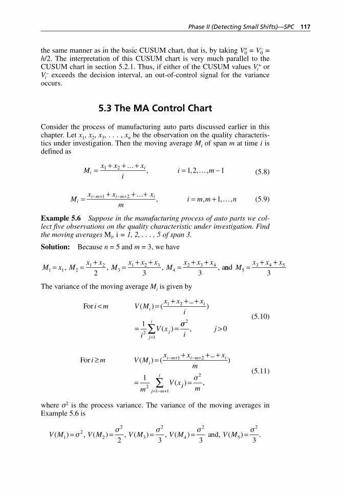
Phase II (Detecting Small Shifts)—SPC 117
the same manner as in the basic CUSUM chart, that is, by taking V0+ = V0
– = h/2. The interpretation of this CUSUM chart is very much parallel to the CUSUM chart in section 5.2.1. Thus, if either of the CUSUM values Vi
+ or Vi
– exceeds the decision interval, an out- of-control signal for the variance occurs.
5.3 The MA Control Chart
Consider the process of manufacturing auto parts discussed earlier in this chapter. Let x1, x2, x3, . . . , xn be the observation on the quality characteris-tics under investigation. Then the moving average Mi of span m at time i is defined as
M
x x x
ii mi
i= + + + = −1 2 1 2 1...
, , , .. . ,
(5.8)
M
x x x
mi m m ni
i m i m i= + + + = +− + − +1 2 1...
, , , . . . ,
(5.9)
Example 5.6 Suppose in the manufacturing process of auto parts we col-lect five observations on the quality characteristic under investigation. Find the moving averages Mi, i = 1, 2, . . . , 5 of span 3.
Solution: Because n = 5 and m = 3, we have
M x Mx x
Mx x x
Mx x x
1 1 21 2
31 2 3
42 3 4
2 3 3= =
+=
+ +=
+ +, , , , annd M
x x x5
3 4 5
3=
+ +
The variance of the moving average Mi is given by
For i m V Mx x x
i
iV x
ii
jj
i
< =+ + +
= ==
∑
( ) (...
)
( )
1 2
21
1 σσ2
0i
j, >
(5.10)
For i m V Mx x x
m
mV x
ii m i m i≥ =
+ + +
=
− + − +( ) (...
)
(
1 2
2
1jj
j m
i
m) ,
= − +∑ =1 1
2σ
(5.11)
where σ2 is the process variance. The variance of the moving averages in Example 5.6 is
V M V M V M V M( ) , ( ) , ( ) , ( )1
22
2
3
2
4
2
2 3 3= = = =σ
σ σ σand, V M( ) .5
2
3=
σ
H1277 ch05.indd 117H1277 ch05.indd 117 3/8/07 12:35:07 PM3/8/07 12:35:07 PM
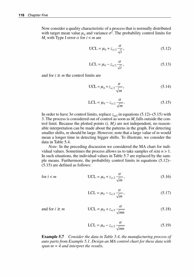
118 Chapter Five
Now consider a quality characteristic of a process that is normally distributed with target mean value µ0 and variance σ2. The probability control limits for Mi with Type I error α for i < m are
UCL = +µ
σα0 2z
i,
(5.12)
LCL = −µ
σα0 2z
i,
(5.13)
and for i ≥ m the control limits are
UCL = +µ
σα0 2z
m,
(5.14)
LCL = −µ
σα0 2z
m.
(5.15)
In order to have 3σ control limits, replace zα/2 in equations (5.12)–(5.15) with 3. The process is considered out of control as soon as Mi falls outside the con-trol limit. Because the plotted points (i, Mi) are not independent, no reason-able interpretation can be made about the patterns in the graph. For detecting smaller shifts, m should be large. However, note that a large value of m would mean a longer time in detecting bigger shifts. To illustrate, we consider the data in Table 5.4.
Note: In the preceding discussion we considered the MA chart for indi-vidual values. Sometimes the process allows us to take samples of size n > 1. In such situations, the individual values in Table 5.7 are replaced by the sam-ple means. Furthermore, the probability control limits in equations (5.12)–(5.15) are defined as follows:
for i < m
UCL = +µσ
α0 2zin
,
(5.16)
LCL = −µ
σα0 2z
in,
(5.17)
and for i ≥ m
UCL = +µσ
α0 2zmn
(5.18)
LCL = −µ
σα0 2z
mn (5.19)
Example 5.7 Consider the data in Table 5.4, the manufacturing process of auto parts from Example 5.1. Design an MA control chart for these data with span m = 4 and interpret the results.
H1277 ch05.indd 118H1277 ch05.indd 118 3/8/07 12:35:08 PM3/8/07 12:35:08 PM
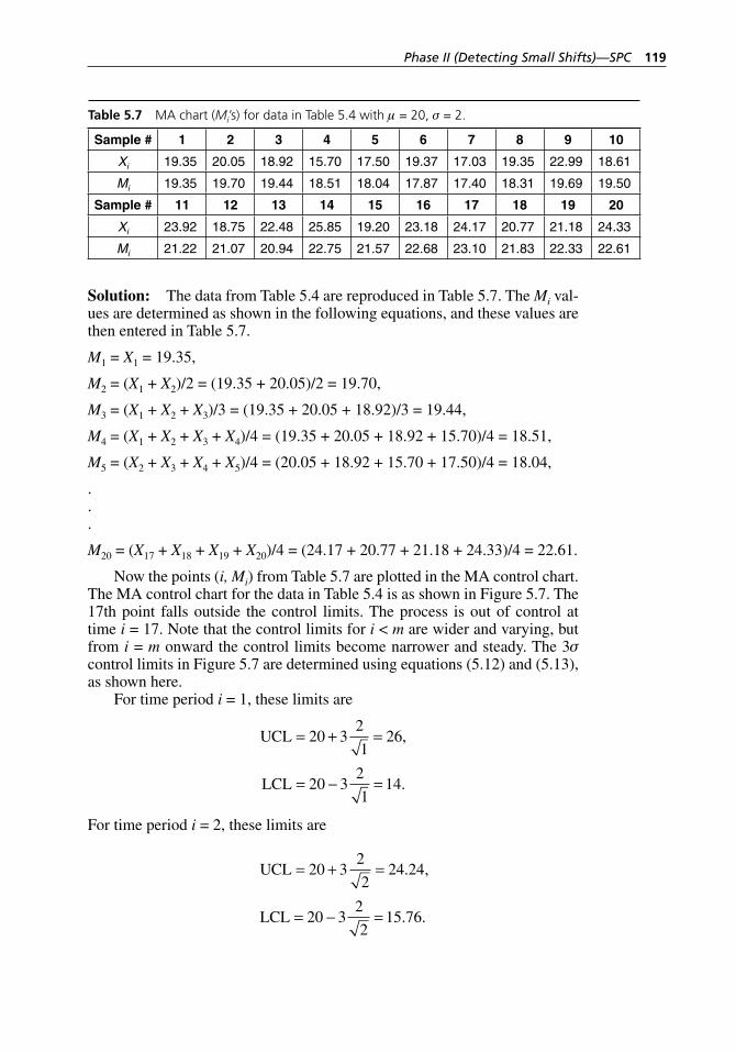
Phase II (Detecting Small Shifts)—SPC 119
Solution: The data from Table 5.4 are reproduced in Table 5.7. The Mi val-ues are determined as shown in the following equations, and these values are then entered in Table 5.7.
M1 = X1 = 19.35,
M2 = (X1 + X2)/2 = (19.35 + 20.05)/2 = 19.70,
M3 = (X1 + X2 + X3)/3 = (19.35 + 20.05 + 18.92)/3 = 19.44,
M4 = (X1 + X2 + X3 + X4)/4 = (19.35 + 20.05 + 18.92 + 15.70)/4 = 18.51,
M5 = (X2 + X3 + X4 + X5)/4 = (20.05 + 18.92 + 15.70 + 17.50)/4 = 18.04,
.
.
.
M20 = (X17 + X18 + X19 + X20)/4 = (24.17 + 20.77 + 21.18 + 24.33)/4 = 22.61.
Now the points (i, Mi) from Table 5.7 are plotted in the MA control chart. The MA control chart for the data in Table 5.4 is as shown in Figure 5.7. The 17th point falls outside the control limits. The process is out of control at time i = 17. Note that the control limits for i < m are wider and varying, but from i = m onward the control limits become narrower and steady. The 3σ control limits in Figure 5.7 are determined using equations (5.12) and (5.13), as shown here.
For time period i = 1, these limits are
UCL
LCL
= + =
= − =
20 32
126
20 32
114
,
.
For time period i = 2, these limits are
UCL
LCL
= + =
= − =
20 32
224 24
20 32
215 76
. ,
. .
Table 5.7 MA chart (Mi’s) for data in Table 5.4 with µ = 20, σ = 2.
Sample # 1 2 3 4 5 6 7 8 9 10
Xi 19.35 20.05 18.92 15.70 17.50 19.37 17.03 19.35 22.99 18.61
Mi 19.35 19.70 19.44 18.51 18.04 17.87 17.40 18.31 19.69 19.50
Sample # 11 12 13 14 15 16 17 18 19 20
Xi 23.92 18.75 22.48 25.85 19.20 23.18 24.17 20.77 21.18 24.33
Mi 21.22 21.07 20.94 22.75 21.57 22.68 23.10 21.83 22.33 22.61
H1277 ch05.indd 119H1277 ch05.indd 119 3/8/07 12:35:08 PM3/8/07 12:35:08 PM
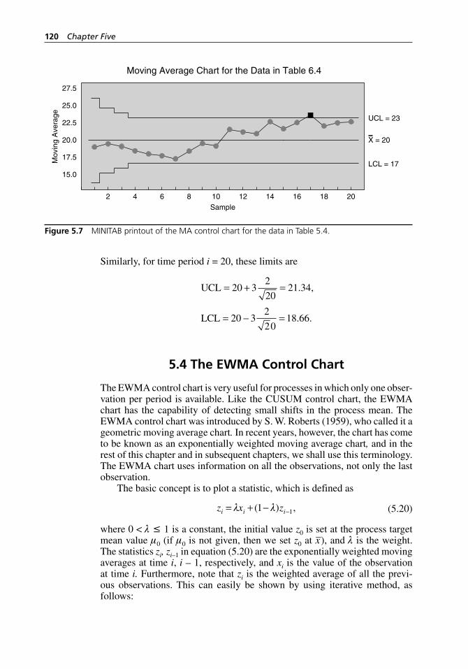
120 Chapter Five
Similarly, for time period i = 20, these limits are
UCL
LCL
= + =
= − =
20 32
2021 34
20 32
2018 66
. ,
. .
5.4 The EWMA Control Chart
The EWMA control chart is very useful for processes in which only one obser-vation per period is available. Like the CUSUM control chart, the EWMA chart has the capability of detecting small shifts in the process mean. The EWMA control chart was introduced by S. W. Roberts (1959), who called it a geometric moving average chart. In recent years, however, the chart has come to be known as an exponentially weighted moving average chart, and in the rest of this chapter and in subsequent chapters, we shall use this terminology. The EWMA chart uses information on all the observations, not only the last observation.
The basic concept is to plot a statistic, which is defined as
z x zi i i= + − −λ λ( ) ,1 1 (5.20)
where 0 < λ ≤ 1 is a constant, the initial value z0 is set at the process target mean value µ0 (if µ0 is not given, then we set z0 at x–), and λ is the weight. The statistics zi, zi–1 in equation (5.20) are the exponentially weighted moving averages at time i, i – 1, respectively, and xi is the value of the observation at time i. Furthermore, note that zi is the weighted average of all the previ-ous observations. This can easily be shown by using iterative method, as follows:
22.5
20.0
15.0
17.5
25.0
27.5
2018161412108642Sample
Mov
ing
Ave
rage
Moving Average Chart for the Data in Table 6.4
UCL = 23
LCL = 17
X = 20
Figure 5.7 MINITAB printout of the MA control chart for the data in Table 5.4.
H1277 ch05.indd 120H1277 ch05.indd 120 3/8/07 12:35:08 PM3/8/07 12:35:08 PM
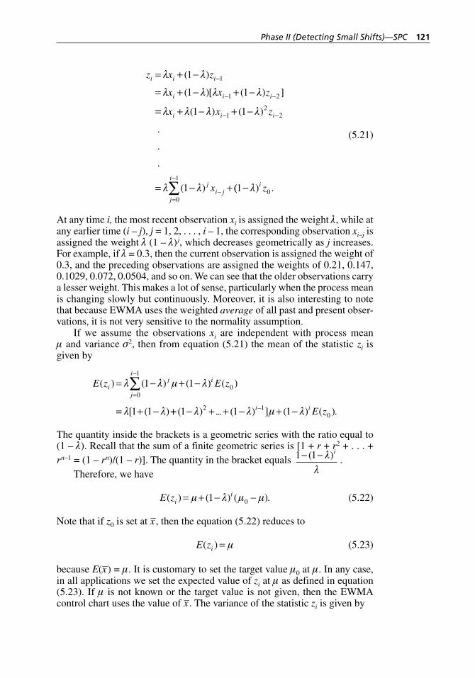
Phase II (Detecting Small Shifts)—SPC 121
z x z
x x z
i i i
i i i
= + −
= + − + −−
− −
λ λ
λ λ λ λ
( )
( )[ ( ) ]
1
1 1
1
1 2
== + − + −
= − +
− −
−
λ λ λ λ
λ λ
x x z
x
i i i
ji j
( ) ( )
.
.
.
( )
1 1
1
12
2
(( ) .1 00
1
−=
−
∑ λ i
j
i
z
(5.21)
At any time i, the most recent observation xi is assigned the weight λ, while at any earlier time (i – j), j = 1, 2, . . . , i – 1, the corresponding observation xi–j is assigned the weight λ (1 – λ) j, which decreases geometrically as j increases. For example, if λ = 0.3, then the current observation is assigned the weight of 0.3, and the preceding observations are assigned the weights of 0.21, 0.147, 0.1029, 0.072, 0.0504, and so on. We can see that the older observations carry a lesser weight. This makes a lot of sense, particularly when the process mean is changing slowly but continuously. Moreover, it is also interesting to note that because EWMA uses the weighted average of all past and present obser-vations, it is not very sensitive to the normality assumption.
If we assume the observations xi are independent with process mean µ and variance σ2, then from equation (5.21) the mean of the statistic zi is given by
E z E zij i
j
i
( ) ( ) ( ) ( )
[ ( )
= − + −
= + −
=
−
∑λ λ µ λ
λ λ
1 1
1 1
00
1
++ − + + − + −−( ) ... ( ) ] ( ) ( ).1 1 12 10λ λ µ λi i E z
The quantity inside the brackets is a geometric series with the ratio equal to (1 – λ). Recall that the sum of a finite geometric series is [1 + r + r2 + . . . + rn–1 = (1 – rn)/(1 – r)]. The quantity in the bracket equals 1 1− −( )λ
λ
i
.Therefore, we have
E zii( ) ( ) ( ).= + − −µ λ µ µ1 0 (5.22)
Note that if z0 is set at x–, then the equation (5.22) reduces to
E zi( ) = µ (5.23)
because E(x–) = µ. It is customary to set the target value µ0 at µ. In any case, in all applications we set the expected value of zi at µ as defined in equation (5.23). If µ is not known or the target value is not given, then the EWMA control chart uses the value of x–. The variance of the statistic zi is given by
H1277 ch05.indd 121H1277 ch05.indd 121 3/8/07 12:35:08 PM3/8/07 12:35:08 PM
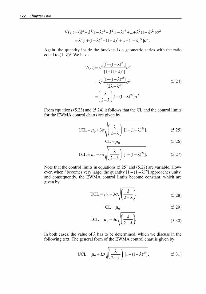
122 Chapter Five
V zii( ) ( ( ) ( ) ... ( ) )= + − + − + + −λ λ λ λ λ λ λ σ2 2 2 2 4 2 21 1 1 22
2 2 4 2 21 1 1 1= + − + − + + −λ λ λ λ σ[ ( ) ( ) ... ( ) ] .i
Again, the quantity inside the brackets is a geometric series with the ratio equal to (1–λ)2. We have
V zi
i
( )[ ( ) ]
[ ( ) ]
[ ( )
=− −− −
=− −
λλ
λσ
λλ
22
22
22
1 1
1 1
1 1 ii
i
]
[ ]
[ ( ) ] .
2
21 1
22
2 2
λ λσ
λ
λλ σ
−
=−
⎛⎝⎜
⎞⎠⎟
− −
(5.24)
From equations (5.23) and (5.24) it follows that the CL and the control limits for the EWMA control charts are given by
UCL = +
−⎛⎝⎜
⎞⎠⎟
− −µ σλ
λλ0
232
1 1[ ( ) ],i
(5.25)
CL = µ0, (5.26)
LCL = −
−⎛⎝⎜
⎞⎠⎟
− −µ σλ
λλ0
232
1 1[ ( ) ].i
(5.27)
Note that the control limits in equations (5.25) and (5.27) are variable. How-ever, when i becomes very large, the quantity [1 – (1 – λ)2i] approaches unity, and consequently, the EWMA control limits become constant, which are given by
UCL = +−
⎛⎝⎜
⎞⎠⎟
µ σλ
λ0 3
2,
(5.28)
CL = µ0, (5.29)
LCL = −−
⎛⎝⎜
⎞⎠⎟
µ σλ
λ0 3
2.
(5.30)
In both cases, the value of λ has to be determined, which we discuss in the following text. The general form of the EWMA control chart is given by
UCL = +
−⎛⎝⎜
⎞⎠⎟ − −µ σ
λλ
λ02
21 1L i[ ( ) ],
(5.31)
H1277 ch05.indd 122H1277 ch05.indd 122 3/8/07 12:35:09 PM3/8/07 12:35:09 PM
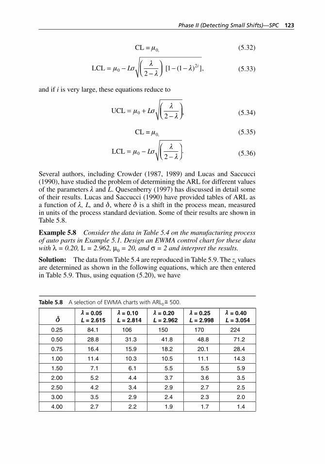
Phase II (Detecting Small Shifts)—SPC 123
CL = µ0, (5.32)
LCL = −−
⎛⎝⎜
⎞⎠⎟ − −µ σ
λλ
λ02
21 1L i[ ( ) ],
(5.33)
and if i is very large, these equations reduce to
UCL = +−
⎛⎝⎜
⎞⎠⎟
µ σλ
λ0
2L ,
(5.34)
CL = µ0, (5.35)
LCL = −−
⎛⎝⎜
⎞⎠⎟
µ σλ
λ0
2L .
(5.36)
Several authors, including Crowder (1987, 1989) and Lucas and Saccucci (1990), have studied the problem of determining the ARL for different values of the parameters λ and L. Quesenberry (1997) has discussed in detail some of their results. Lucas and Saccucci (1990) have provided tables of ARL as a function of λ, L, and δ, where δ is a shift in the process mean, measured in units of the process standard deviation. Some of their results are shown in Table 5.8.
Example 5.8 Consider the data in Table 5.4 on the manufacturing process of auto parts in Example 5.1. Design an EWMA control chart for these data with λ = 0.20, L = 2.962, µ0 = 20, and σ = 2 and interpret the results.
Solution: The data from Table 5.4 are reproduced in Table 5.9. The zi values are determined as shown in the following equations, which are then entered in Table 5.9. Thus, using equation (5.20), we have
Table 5.8 A selection of EWMA charts with ARL0~= 500.
= 0.05 L = 2.615
= 0.10 L = 2.814
= 0.20 L = 2.962
= 0.25 L = 2.998
= 0.40 L = 3.054
0.25 84.1 106 150 170 224
0.50 28.8 31.3 41.8 48.8 71.2
0.75 16.4 15.9 18.2 20.1 28.4
1.00 11.4 10.3 10.5 11.1 14.3
1.50 7.1 6.1 5.5 5.5 5.9
2.00 5.2 4.4 3.7 3.6 3.5
2.50 4.2 3.4 2.9 2.7 2.5
3.00 3.5 2.9 2.4 2.3 2.0
4.00 2.7 2.2 1.9 1.7 1.4
H1277 ch05.indd 123H1277 ch05.indd 123 3/8/07 12:35:09 PM3/8/07 12:35:09 PM
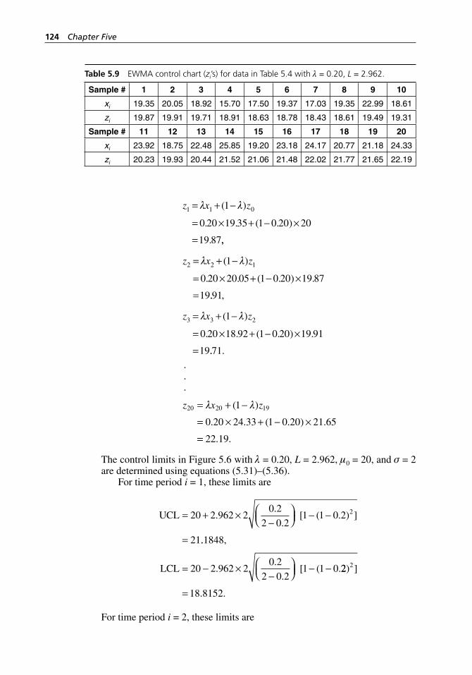
124 Chapter Five
z x z1 1 01
0 20 19 35 1 0 20 20
19 87
= + −
= × + − ×
=
λ λ( )
. . ( . )
. ,,
z x z2 2 11
0 20 20 05 1 0 20 19 87
19
= + −
= × + − ×
=
λ λ( )
. . ( . ) .
.. ,91
z x z3 3 21
0 20 18 92 1 0 20 19 91
19
= + −
= × + − ×
=
λ λ( )
. . ( . ) .
.. .71 . . .
z x z20 20 191
0 20 24 33 1 0 20 21 65
= + −
= × + − ×
λ λ( )
. . ( . ) .
== 22 19. .
The control limits in Figure 5.6 with λ = 0.20, L = 2.962, µ0 = 20, and σ = 2 are determined using equations (5.31)–(5.36).
For time period i = 1, these limits are
UCL = + ×−
⎛⎝⎜
⎞⎠⎟ − −
=
20 2 962 20 2
2 0 21 1 0 2
21
2..
.[ ( . ) ]
.. ,
..
.[ ( .
1848
20 2 962 20 2
2 0 21 1 0LCL = − ×
−⎛⎝⎜
⎞⎠⎟ − − 22
18 8152
2) ]
. .=
For time period i = 2, these limits are
Table 5.9 EWMA control chart (zi’s) for data in Table 5.4 with λ = 0.20, L = 2.962.
Sample # 1 2 3 4 5 6 7 8 9 10
xi 19.35 20.05 18.92 15.70 17.50 19.37 17.03 19.35 22.99 18.61
zi 19.87 19.91 19.71 18.91 18.63 18.78 18.43 18.61 19.49 19.31
Sample # 11 12 13 14 15 16 17 18 19 20
xi 23.92 18.75 22.48 25.85 19.20 23.18 24.17 20.77 21.18 24.33
zi 20.23 19.93 20.44 21.52 21.06 21.48 22.02 21.77 21.65 22.19
H1277 ch05.indd 124H1277 ch05.indd 124 3/8/07 12:35:09 PM3/8/07 12:35:09 PM
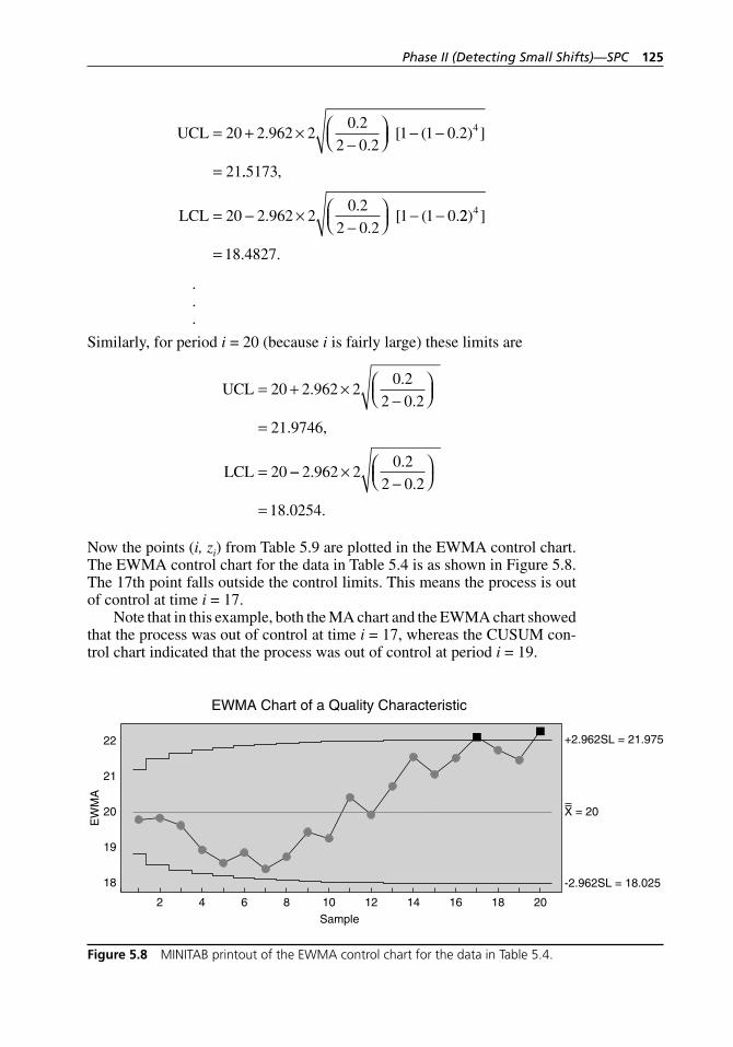
Phase II (Detecting Small Shifts)—SPC 125
UCL = + ×−
⎛⎝⎜
⎞⎠⎟ − −
=
20 2 962 20 2
2 0 21 1 0 2
21
4..
.[ ( . ) ]
.. ,
..
.[ ( .
5173
20 2 962 20 2
2 0 21 1 0LCL = − ×
−⎛⎝⎜
⎞⎠⎟ − − 22
18 4827
4) ]
. .=
. . .
Similarly, for period i = 20 (because i is fairly large) these limits are
UCL
LCL
= + ×−
⎛⎝⎜
⎞⎠⎟
=
=
20 2 962 20 2
2 0 2
21 9746
20
..
.
. ,
−− ×−
⎛⎝⎜
⎞⎠⎟
=
2 962 20 2
2 0 2
18 0254
..
.
. .
Now the points (i, zi) from Table 5.9 are plotted in the EWMA control chart. The EWMA control chart for the data in Table 5.4 is as shown in Figure 5.8. The 17th point falls outside the control limits. This means the process is out of control at time i = 17.
Note that in this example, both the MA chart and the EWMA chart showed that the process was out of control at time i = 17, whereas the CUSUM con-trol chart indicated that the process was out of control at period i = 19.
20
19
18
21
22
2018161412108642Sample
EW
MA
EWMA Chart of a Quality Characteristic
+2.962SL = 21.975
-2.962SL = 18.025
X = 20
Figure 5.8 MINITAB printout of the EWMA control chart for the data in Table 5.4.
H1277 ch05.indd 125H1277 ch05.indd 125 3/8/07 12:35:09 PM3/8/07 12:35:09 PM

H1277 ch05.indd 126H1277 ch05.indd 126 3/8/07 12:35:10 PM3/8/07 12:35:10 PM
127
In Chapter 3 we defined a process as a series of actions or operations performed in producing manufactured or nonmanufactured products. A process may also be defined as a combination of workforce, equipment,
raw materials, methods, and environment that works together to produce out-put. Figure 6.1, which was presented earlier as Figure 3.1, shows where each component of a process fits.
The quality of the final product depends on how the process is designed and executed. However, no matter how perfectly a process is designed or how well it is executed, no two items produced by the process are identical. The difference between two items is called the variation. Such variation occurs because of two causes:
1. Common causes or random causes
2. Special causes or assignable causes
Shewhart was the first to attempt to understand and remove variation in a very systematic way, in 1924 when he presented the graph of a control chart. In Chapters 3, 4, and 5 we studied various types of control charts, includ-ing Shewhart control charts, and noted that they help bring the process into control. Recall that a process is brought into control by eliminating special or assignable causes so that the process contains only common or random causes, and consequently, the process is stable and thus predictable. To study process capability, it is essential that the process is stable; otherwise, study-ing process capability is simply a futile exercise.
6.1 Development of Process Capability Indices
Once the process is under statistical control and thus predictable, the next concern of a manufacturer is to ensure that he or she can deliver the prod-uct the consumer wants. In other words, the manufacturer wants to determine whether the process is capable of delivering the desired product. One way to
6
Process Capability Indices
H1277 ch06.indd 127H1277 ch06.indd 127 3/8/07 12:36:31 PM3/8/07 12:36:31 PM
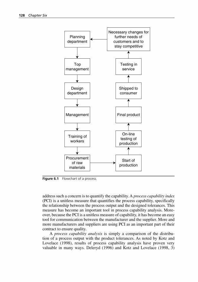
128 Chapter Six
address such a concern is to quantify the capability. A process capability index (PCI) is a unitless measure that quantifies the process capability, specifically the relationship between the process output and the designed tolerances. This measure has become an important tool in process capability analysis. More-over, because the PCI is a unitless measure of capability, it has become an easy tool for communication between the manufacturer and the supplier. More and more manufacturers and suppliers are using PCI as an important part of their contract to ensure quality.
A process capability analysis is simply a comparison of the distribu-tion of a process output with the product tolerances. As noted by Kotz and Lovelace (1998), results of process capability analysis have proven very valuable in many ways. Deleryd (1996) and Kotz and Lovelace (1998, 3)
On-linetesting of
production
Start ofproduction
Necessary changes forfurther needs of
customers and tostay competitive
Final product
Shipped toconsumer
Testing inservice
Planningdepartment
Topmanagement
Designdepartment
Management
Training ofworkers
Procurementof raw
materials
Figure 6.1 Flowchart of a process.
H1277 ch06.indd 128H1277 ch06.indd 128 3/8/07 12:36:31 PM3/8/07 12:36:31 PM
Process Capability Indices 129
developed a list of the 13 most common ways of using the results of process capability analysis:
1. As a basis in the improvement process.
2. As an alarm clock.
3. As specifications for investments. By giving specifications for levels of PCIs expected to be reached by new machines, the purchasing process is facilitated.
4. As a certificate for customers. The supplier is able to attach with the delivery the results from the process capability studies conducted when the actual products were produced.
5. As a basis for new constructions. By knowing the capability of the production processes, the designer knows how to set reasonable specifications in order to make the product manufacturable.
6. For control of maintenance efforts. By continuously conducting process capability studies, it is possible to see if some machines are gradually deteriorating.
7. As specifications for introducing new products.
8. For assessing reasonableness of customer demands.
9. For motivation of coworkers.
10. For deciding priorities in the improvement process.
11. As a base for inspection activities.
12. As a receipt for improvement.
13. For formulating quality improvement programs.
To implement a process capability analysis, one needs to consider the following:
1. The target value specification, which is usually defined by the customer.
2. The specification limits, which should be defined by the customer or the customer’s technical staff and agreed upon by the manufacturer. Furthermore, the specification limits should be such that they allow manufacturing variability without jeopardizing proper function of the product.
3. An analysis of the process that would allow the manufacturer to determine whether the product can meet the customer’s specifications.
Once production starts, the manufacturer conducts capability studies to com-pare the measures of the quality characteristic of the manufactured product with the specification limits. This is where PCIs are used.
H1277 ch06.indd 129H1277 ch06.indd 129 3/8/07 12:36:32 PM3/8/07 12:36:32 PM
130 Chapter Six
The first- generation PCIs were established by Japanese manufacturers in the 1970s. They used the following indices:
Cp—Inherent capability of a process
k—Position of the process in relation to the target value
Cpk—Position of the 6σ process in relation to the target value
Cpl—Position of the 6σ process in relation to the LSL
Cpu—Position of the 6σ process in relation to the USL
In this chapter we will study these and various other capability indices fre-quently used in process capability analysis. This book does not cover every aspect of these indices. However, an excellent reference for a more detailed study is Kotz and Lovelace (1998).
Throughout the study of these indices, we are going to assume that the process producing the desired quality characteristic is under control and thus predictable.
6.2 PCI Cp
Let X be the process quality characteristic we want to monitor. Let USL and LSL be the upper specification limit and lower specification limit, respec-tively. The performance of the process with respect to these limits is defined as follows:
Percentage of nonconforming produced by the process at the upper end = P(X > USL),
Percentage of nonconforming produced by the process at the lower end = P(X < LSL).
The total percentage of nonconforming products produced by the process is defined as
P(X < LSL or X > USL) = 1 – P(LSL < X < USL).
In the preceding paragraph we saw the performance of the process with respect to the specification limits. Now we will look at the performance of the process with respect to the natural tolerance limits (NTLs), that is, the UNTL and the LNTL.
The performance of the process with respect to the NTLs is the percent-age of the product produced by the process with its quality characteristic falling within the interval (µ – 3σ, µ + 3σ), where µ and σ, respectively, are the mean and the standard deviation of the process quality characteristic. Assuming that the process quality characteristic is normally distributed and that the process is under control, the percentage of the product produced by the process with its quality characteristic falling within the interval (µ – 3σ, µ + 3σ) is approximately 99.74 percent. As noted earlier, a PCI is the com-parison between what a process is expected to produce and what it is actually
H1277 ch06.indd 130H1277 ch06.indd 130 3/8/07 12:36:32 PM3/8/07 12:36:32 PM
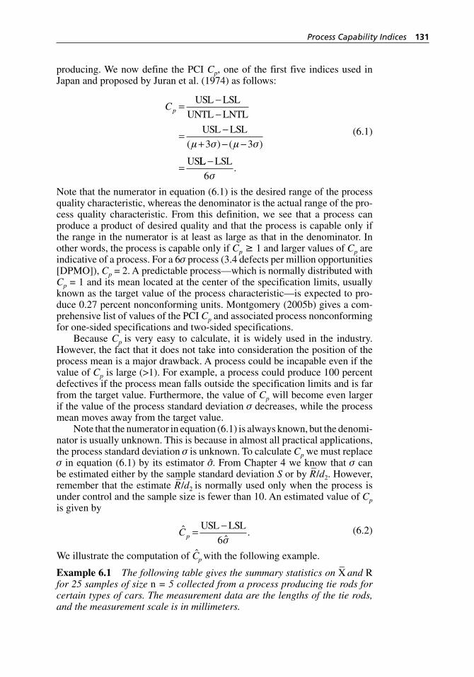
Process Capability Indices 131
producing. We now define the PCI Cp, one of the first five indices used in Japan and proposed by Juran et al. (1974) as follows:
Cp =−−
=−
+ − −
=
USL LSL
UNTL LNTL
USL LSL
US
( ) ( )µ σ µ σ3 3
LL LSL−6σ
.
(6.1)
Note that the numerator in equation (6.1) is the desired range of the process quality characteristic, whereas the denominator is the actual range of the pro-cess quality characteristic. From this definition, we see that a process can produce a product of desired quality and that the process is capable only if the range in the numerator is at least as large as that in the denominator. In other words, the process is capable only if Cp ≥ 1 and larger values of Cp are indicative of a process. For a 6σ process (3.4 defects per million opportunities [DPMO]), Cp = 2. A predictable process—which is normally distributed with Cp = 1 and its mean located at the center of the specification limits, usually known as the target value of the process characteristic—is expected to pro-duce 0.27 percent nonconforming units. Montgomery (2005b) gives a com-prehensive list of values of the PCI Cp and associated process nonconforming for one- sided specifications and two- sided specifications.
Because Cp is very easy to calculate, it is widely used in the industry. However, the fact that it does not take into consideration the position of the process mean is a major drawback. A process could be incapable even if the value of Cp is large (>1). For example, a process could produce 100 percent defectives if the process mean falls outside the specification limits and is far from the target value. Furthermore, the value of Cp will become even larger if the value of the process standard deviation σ decreases, while the process mean moves away from the target value.
Note that the numerator in equation (6.1) is always known, but the denomi-nator is usually unknown. This is because in almost all practical applications, the process standard deviation σ is unknown. To calculate Cp we must replace σ in equation (6.1) by its estimator σ. From Chapter 4 we know that σ can be estimated either by the sample standard deviation S or by R
–/d2. However,
remember that the estimate R–/d2 is normally used only when the process is
under control and the sample size is fewer than 10. An estimated value of Cp is given by
ˆ
ˆ.Cp =
−USL LSL
6σ (6.2)
We illustrate the computation of Cp with the following example.
Example 6.1 The following table gives the summary statistics on X– and R
for 25 samples of size n = 5 collected from a process producing tie rods for certain types of cars. The measurement data are the lengths of the tie rods, and the measurement scale is in millimeters.
H1277 ch06.indd 131H1277 ch06.indd 131 3/8/07 12:36:32 PM3/8/07 12:36:32 PM
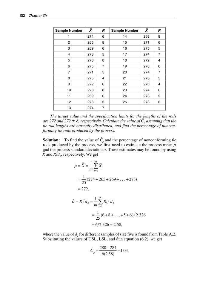
132 Chapter Six
Sample Number X–
R Sample Number X–
R
1 274 6 14 268 8
2 265 8 15 271 6
3 269 6 16 275 5
4 273 5 17 274 7
5 270 8 18 272 4
6 275 7 19 270 6
7 271 5 20 274 7
8 275 4 21 273 5
9 272 6 22 270 4
10 273 8 23 274 6
11 269 6 24 273 5
12 273 5 25 273 6
13 274 7
The target value and the specification limits for the lengths of the rods are 272 and 272 ± 8, respectively. Calculate the value of Cp assuming that the tie rod lengths are normally distributed, and find the percentage of noncon-forming tie rods produced by the process.
Solution: To find the value of Cp and the percentage of nonconforming tie rods produced by the process, we first need to estimate the process mean µ and the process standard deviation σ. These estimates may be found by using –X– and R
–/d2, respectively. We get
ˆ
(
,
Xm
Xii
m1
1
25274 265 269 273
272
1
. . . )
5 6
ˆ
( .
.
R dm
R dii
m
21
21
125
6 8 2 326
6 2 3226 2 58. ,
. . . )
where the value of d2 for different samples of size five is found from Table A.2. Substituting the values of USL, LSL, and σ in equation (6.2), we get
ˆ( . )
. ,Cp =−
=280 284
6 2 581 03
H1277 ch06.indd 132H1277 ch06.indd 132 3/8/07 12:36:32 PM3/8/07 12:36:32 PM
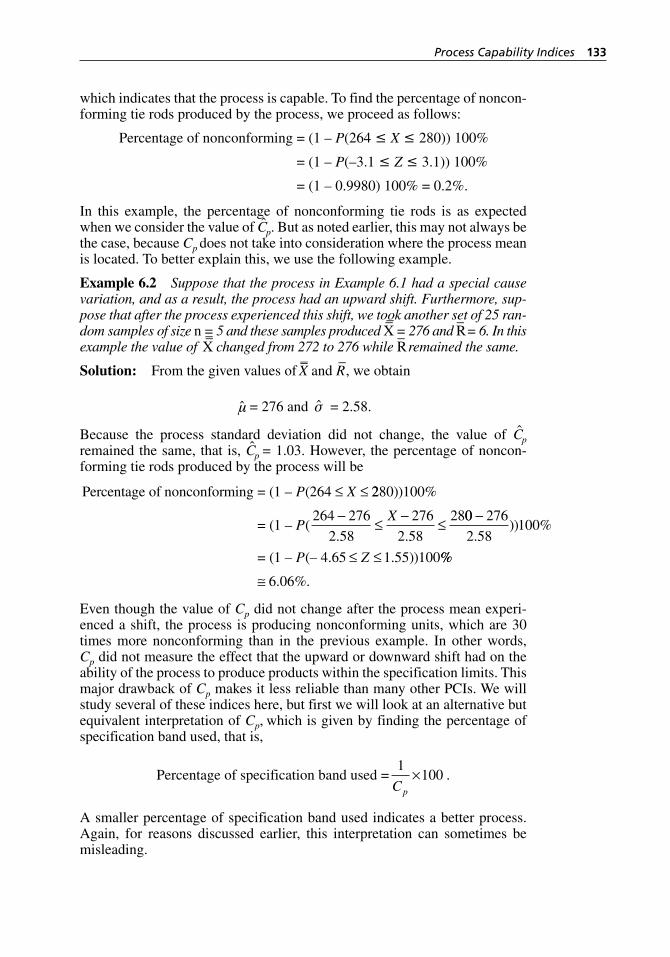
Process Capability Indices 133
which indicates that the process is capable. To find the percentage of noncon-forming tie rods produced by the process, we proceed as follows:
Percentage of nonconforming = (1 – P(264 ≤ X ≤ 280)) 100%
= (1 – P(–3.1 ≤ Z ≤ 3.1)) 100%
= (1 – 0.9980) 100% = 0.2%.
In this example, the percentage of nonconforming tie rods is as expected when we consider the value of Cp. But as noted earlier, this may not always be the case, because Cp does not take into consideration where the process mean is located. To better explain this, we use the following example.
Example 6.2 Suppose that the process in Example 6.1 had a special cause variation, and as a result, the process had an upward shift. Furthermore, sup-pose that after the process experienced this shift, we took another set of 25 ran-dom samples of size n = 5 and these samples produced
–X–
= 276 and R– = 6. In this
example the value of –X– changed from 272 to 276 while R
– remained the same.
Solution: From the given values of –X– and R
–, we obtain
µ = 276 and σ = 2.58.
Because the process standard deviation did not change, the value of Cp remained the same, that is, Cp = 1.03. However, the percentage of noncon-forming tie rods produced by the process will be
Percentage of nonconforming = (1 – (264P X≤ ≤ 2280))100%
= (1 – (PX264 276
2 58
276
2 58
28− ≤ − ≤. .
00 276
2 58100
−
≤ ≤.
)) %
= (1 – (– 4.65 1.55))100P Z %%
6.06%.≅
Even though the value of Cp did not change after the process mean experi-enced a shift, the process is producing nonconforming units, which are 30 times more nonconforming than in the previous example. In other words, Cp did not measure the effect that the upward or downward shift had on the ability of the process to produce products within the specification limits. This major drawback of Cp makes it less reliable than many other PCIs. We will study several of these indices here, but first we will look at an alternative but equivalent interpretation of Cp, which is given by finding the percentage of specification band used, that is,
Percentage of specification band used =1
100Cp
× .
A smaller percentage of specification band used indicates a better process. Again, for reasons discussed earlier, this interpretation can sometimes be misleading.
H1277 ch06.indd 133H1277 ch06.indd 133 3/8/07 12:36:33 PM3/8/07 12:36:33 PM
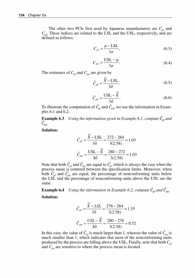
134 Chapter Six
The other two PCIs first used by Japanese manufacturers are Cpl and Cpu. These indices are related to the LSL and the USL, respectively, and are defined as follows:
Cpl =
−µ
σ
LSL
3,
(6.3)
Cpu =
−USL µ
σ3.
(6.4)
The estimates of Cpl and Cpu are given by
ˆ
ˆ,C
Xpl =
− LSL
3σ (6.5)
ˆ
ˆ.C
Xpu =
−USL
3σ (6.6)
To illustrate the computation of Cpl and Cpu, we use the information in Exam-ples 6.1 and 6.2.
Example 6.3 Using the information given in Example 6.1, compute Cpl and Cpu.
Solution:
ˆˆ ( . )
.
ˆ
CX
CX
pl
pu
=−
=−
=
=−
LSL
USL
3
272 264
3 2 581 03
σ
33
280 272
3 2 581 03
ˆ ( . ).
σ=
−=
Note that both Cpl and Cpu are equal to Cp, which is always the case when the process mean is centered between the specification limits. Moreover, when both Cpl and Cpu are equal, the percentage of nonconforming units below the LSL and the percentage of nonconforming units above the USL are the same.
Example 6.4 Using the information in Example 6.2, compute Cpl and Cpu.
Solution:
ˆˆ ( . )
.
ˆ
CX LSL
CUSL X
pl
pu
=−
=−
=
=−
3
276 264
3 2 581 55
σ
33
280 276
3 2 580 52
ˆ ( . ).
σ=
−=
In this case, the value of Cpl is much larger than 1, whereas the value of Cpu is much smaller than 1, which indicates that most of the nonconforming units produced by the process are falling above the USL. Finally, note that both Cpl and Cpu are sensitive to where the process mean is located.
H1277 ch06.indd 134H1277 ch06.indd 134 3/8/07 12:36:33 PM3/8/07 12:36:33 PM
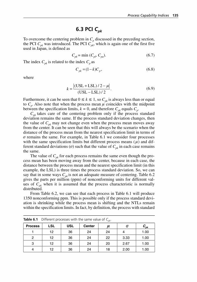
Process Capability Indices 135
6.3 PCI Cpk
To overcome the centering problem in Cp discussed in the preceding section, the PCI Cpk was introduced. The PCI Cpk, which is again one of the first five used in Japan, is defined as
Cpk = min (Cpl, Cpu). (6.7)
The index Cpk is related to the index Cp as
C k Cpk p= −( ) ,1
(6.8)
where
k =
+ −−
( ) /
( ) /.
USL LSL
USL LSL
2
2
µ
(6.9)
Furthermore, it can be seen that 0 ≤ k ≤ 1, so Cpk is always less than or equal to Cp. Also note that when the process mean µ coincides with the midpoint between the specification limits, k = 0, and therefore Cpk equals Cp.
Cpk takes care of the centering problem only if the process standard deviation remains the same. If the process standard deviation changes, then the value of Cpk may not change even when the process mean moves away from the center. It can be seen that this will always be the scenario when the distance of the process mean from the nearest specification limit in terms of σ remains the same. For example, in Table 6.1 we consider four processes with the same specification limits but different process means ( µ) and dif-ferent standard deviations (σ) such that the value of Cpk in each case remains the same.
The value of Cpk for each process remains the same even though the pro-cess mean has been moving away from the center, because in each case, the distance between the process mean and the nearest specification limit (in this example, the LSL) is three times the process standard deviation. So, we can say that in some ways Cpk is not an adequate measure of centering. Table 6.2 gives the parts per million (ppm) of nonconforming units for different val-ues of Cpk when it is assumed that the process characteristic is normally distributed.
From Table 6.2, we can see that each process in Table 6.1 will produce 1350 nonconforming ppm. This is possible only if the process standard devi-ation is shrinking while the process mean is shifting and the NTLs remain within the specification limits. In fact, by definition, the process with standard
Table 6.1 Different processes with the same value of Cpk.
Process LSL USL Center Cpk
1 12 36 24 24 4 1.00
2 12 36 24 22 3.33 1.00
3 12 36 24 20 2.67 1.00
4 12 36 24 18 2.00 1.00
H1277 ch06.indd 135H1277 ch06.indd 135 3/8/07 12:36:33 PM3/8/07 12:36:33 PM
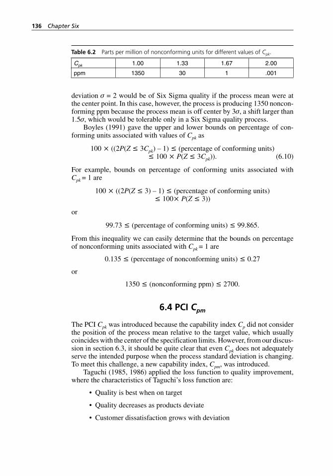
136 Chapter Six
deviation σ = 2 would be of Six Sigma quality if the process mean were at the center point. In this case, however, the process is producing 1350 noncon-forming ppm because the process mean is off center by 3σ, a shift larger than 1.5σ, which would be tolerable only in a Six Sigma quality process.
Boyles (1991) gave the upper and lower bounds on percentage of con-forming units associated with values of Cpk as
100 × ((2P(Z ≤ 3Cpk) – 1) ≤ (percentage of conforming units) ≤ 100 × P(Z ≤ 3Cpk)). (6.10)
For example, bounds on percentage of conforming units associated with Cpk = 1 are
100 × ((2P(Z ≤ 3) – 1) ≤ (percentage of conforming units) ≤ 100× P(Z ≤ 3))
or
99.73 ≤ (percentage of conforming units) ≤ 99.865.
From this inequality we can easily determine that the bounds on percentage of nonconforming units associated with Cpk = 1 are
0.135 ≤ (percentage of nonconforming units) ≤ 0.27
or
1350 ≤ (nonconforming ppm) ≤ 2700.
6.4 PCI Cpm
The PCI Cpk was introduced because the capability index Cp did not consider the position of the process mean relative to the target value, which usually coincides with the center of the specification limits. However, from our discus-sion in section 6.3, it should be quite clear that even Cpk does not adequately serve the intended purpose when the process standard deviation is changing. To meet this challenge, a new capability index, Cpm, was introduced.
Taguchi (1985, 1986) applied the loss function to quality improvement, where the characteristics of Taguchi’s loss function are:
Quality is best when on target
Quality decreases as products deviate
Customer dissatisfaction grows with deviation
•
•
•
Table 6.2 Parts per million of nonconforming units for different values of Cpk.
Cpk 1.00 1.33 1.67 2.00
ppm 1350 30 1 .001
H1277 ch06.indd 136H1277 ch06.indd 136 3/8/07 12:36:34 PM3/8/07 12:36:34 PM
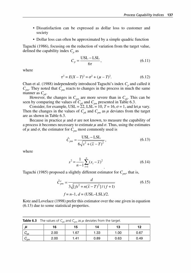
Process Capability Indices 137
Dissatisfaction can be expressed as dollar loss to customer and society
Dollar loss can often be approximated by a simple quadric function
Taguchi (1986), focusing on the reduction of variation from the target value, defined the capability index Cp as
Cp =
−USL LSL
6τ,
(6.11)
where
τ2 = E(X – T)2 = σ2 + ( µ – T)2. (6.12)
Chan et al. (1988) independently introduced Taguchi’s index Cp and called it Cpm. They noted that Cpm reacts to changes in the process in much the same manner as Cpk.
However, the changes in Cpm are more severe than in Cpk. This can be seen by comparing the values of Cpk and Cpm presented in Table 6.3.
Consider, for example, USL = 22, LSL = 10, T = 16, σ = 1, and let µ vary. Then the changes in the values of Cpk and Cpm as µ deviates from the target are as shown in Table 6.3.
Because in practice µ and σ are not known, to measure the capability of a process it becomes necessary to estimate µ and σ. Thus, using the estimates of µ and σ, the estimator for Cpm most commonly used is
ˆ( )
,Cs x T
pm =−
+ −
USL LSL
6 2 2
(6.13)
where
s
nx xi
i
n2 2
1
1
1=
−−
=∑( )
. (6.14)
Taguchi (1985) proposed a slightly different estimator for Cpm, that is,
ˆ[ ( ) ] / ( )
′ =+ − +
Cd
fs n x T fpm
3 12 2
(6.15)
f = n–1, d = (USL–LSL)/2.
Kotz and Lovelace (1998) prefer this estimator over the one given in equation (6.13) due to some statistical properties.
•
•
Table 6.3 The values of Cpk and Cpm as µ deviates from the target.
16 15 14 13 12
Cpk 2.00 1.67 1.33 1.00 0.67
Cpm 2.00 1.41 0.89 0.63 0.49
H1277 ch06.indd 137H1277 ch06.indd 137 3/8/07 12:36:34 PM3/8/07 12:36:34 PM
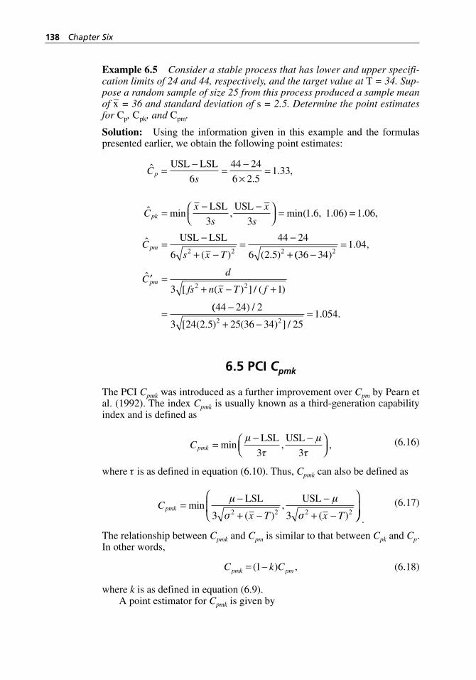
138 Chapter Six
Example 6.5 Consider a stable process that has lower and upper specifi-cation limits of 24 and 44, respectively, and the target value at T = 34. Sup-pose a random sample of size 25 from this process produced a sample mean of x– = 36 and standard deviation of s = 2.5. Determine the point estimates for Cp, Cpk, and Cpm.
Solution: Using the information given in this example and the formulas presented earlier, we obtain the following point estimates:
ˆ
.. ,C
sp =
−=
−×
=USL LSL
6
44 24
6 2 51 33
ˆ , ( . , . )Cx
s
x
spk =
− −⎛⎝⎜
⎞⎠⎟ =min
LSL USLmin
3 31 6 1 06 ==
=−
+ −=
−
+
1 06
6
44 24
6 2 52 2 2
. ,
ˆ( ) ( . )
Cs x T
pmUSL LSL
(( ). ,
ˆ[ ( ) ] / ( )
36 341 04
3 1
2
2 2
−=
′ =+ − +
=
Cd
fs n x T fpm
(( ) /
[ ( . ) ( ) ] /. .
44 24 2
3 24 2 5 25 36 34 251 054
2 2
−
+ −=
6.5 PCI Cpmk
The PCI Cpmk was introduced as a further improvement over Cpm by Pearn et al. (1992). The index Cpmk is usually known as a third- generation capability index and is defined as
Cpmk =
− −⎛⎝⎜
⎞⎠⎟min
LSL USLµ
τ
µ
τ3 3, ,
(6.16)
where τ is as defined in equation (6.10). Thus, Cpmk can also be defined as
C
x T x Tpmk =
−
+ −
−
+ −
⎛
⎝⎜
⎞min
LSL USLµ
σ
µ
σ3 32 2 2 2( ),
( ) ⎠⎠⎟
.
(6.17)
The relationship between Cpmk and Cpm is similar to that between Cpk and Cp. In other words,
C k Cpmk pm= −( ) ,1
(6.18)
where k is as defined in equation (6.9).A point estimator for Cpmk is given by
H1277 ch06.indd 138H1277 ch06.indd 138 3/8/07 12:36:34 PM3/8/07 12:36:34 PM
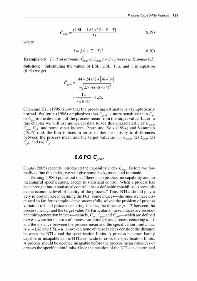
Process Capability Indices 139
ˆ ( ) /
ˆ,C
x Tpmk =
− + −USL LSL 2
3τ (6.19)
where
ˆ ( )τ = + −s x T2 2 . (6.20)
Example 6.6 Find an estimator Cpmk of Cpmk for the process in Example 6.5.
Solution: Substituting the values of LSL, USL, T, s, and x– in equation (6.19) we get
ˆ ( ) /
. ( )
.
Cpmk =− + −
+ −
=
44 24 2 36 34
3 2 5 36 34
12
3 10 2
2 2
551 25= . .
Chen and Hsu (1995) show that the preceding estimator is asymptotically normal. Wallgren (1996) emphasizes that Cpmk is more sensitive than Cpk or Cpm to the deviation of the process mean from the target value. Later in this chapter we will use numerical data to see this characteristic of Cpmk, Cpm, Cpk, and some other indices. Pearn and Kotz (1994) and Vännman (1995) rank the four indices in terms of their sensitivity to differences between the process mean and the target value as (1) Cpmk, (2) Cpm, (3) Cpk, and (4) Cp.
6.6 PCI Cpnst
Gupta (2005) recently introduced the capability index Cpnst. Before we for-mally define this index, we will give some background and rationale.
Deming (1986) points out that “there is no process, no capability and no meaningful specifications, except in statistical control. When a process has been brought into a statistical control it has a definable capability, expressible as the economic level of quality of the process.” Thus, NTLs should play a very important role in defining the PCI. Some indices—the ones we have dis-cussed so far, for example—have successfully solved the problem of process variation (σ) and process centering (that is, the distance µ – T between the process mean µ and the target value T). Particularly, these indices are second- and third- generation indices—namely, Cpk, Cpm, and Cpmk—which are defined as we saw earlier in terms of process variation (σ) and process centering µ – T and the distance between the process mean and the specification limits, that is, µ – LSL and USL – µ. However, none of these indices consider the distance between the NTLs and the specification limits. A process becomes barely capable or incapable as the NTLs coincide or cross the specification limits. A process should be deemed incapable before the process mean coincides or crosses the specification limits. Once the position of the NTLs is determined
H1277 ch06.indd 139H1277 ch06.indd 139 3/8/07 12:36:34 PM3/8/07 12:36:34 PM
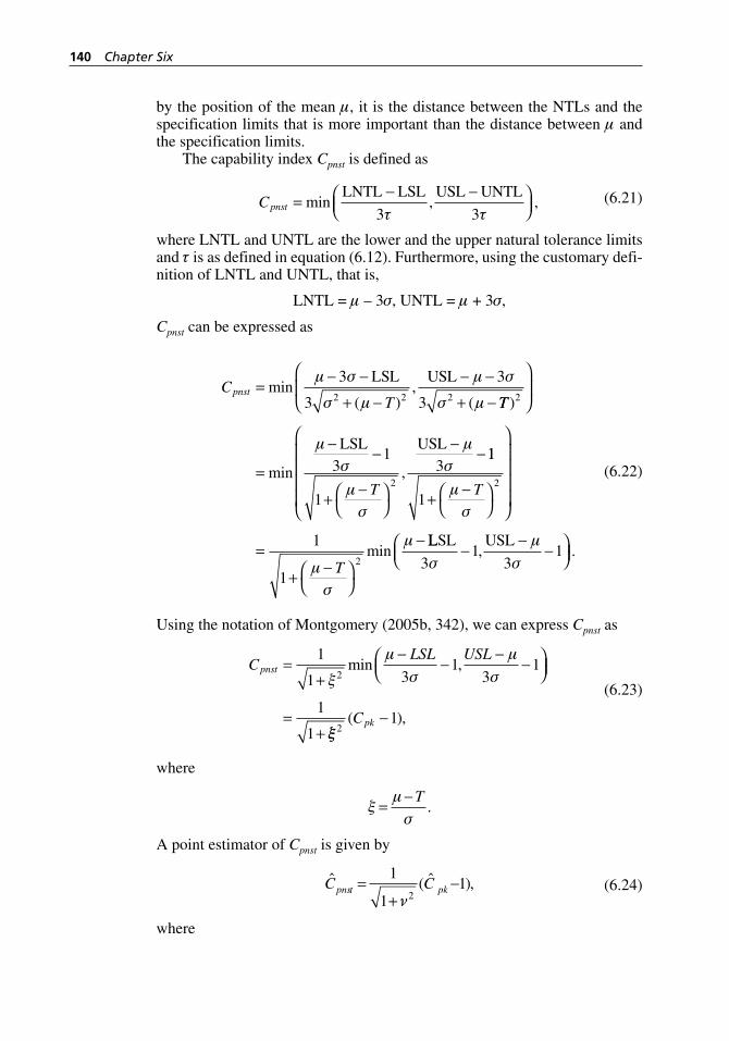
140 Chapter Six
by the position of the mean µ, it is the distance between the NTLs and the specification limits that is more important than the distance between µ and the specification limits.
The capability index Cpnst is defined as
Cpnst =
− −⎛⎝⎜
⎞⎠⎟min , ,
LNTL LSL USL UNTL
3 3τ τ (6.21)
where LNTL and UNTL are the lower and the upper natural tolerance limits and τ is as defined in equation (6.12). Furthermore, using the customary defi-nition of LNTL and UNTL, that is,
LNTL = µ – 3σ, UNTL = µ + 3σ,
Cpnst can be expressed as
CT
pnst =− −
+ −
− −
+ −min
( ),
(
µ σ
σ µ
µ σ
σ µ
3
3
3
32 2 2
LSL USL
TT
T
)
min ,
2
2
31
1
3
⎛
⎝⎜
⎞
⎠⎟
=
− −
+ −⎛⎝
⎞⎠
− −µσ
µσ
µσ
LSL USL11
1
1
1
2
2
+ −⎛⎝
⎞⎠
⎛
⎝
⎜⎜⎜⎜
⎞
⎠
⎟⎟⎟⎟
=
+ −⎛⎝
⎞⎠
−
µσ
µσ
µ
T
Tmin
LLSL USL
31
31
σ
µ
σ−
−−⎛
⎝⎜⎞⎠⎟, .
(6.22)
Using the notation of Montgomery (2005b, 342), we can express Cpnst as
CLSL USL
pnst =+
−−
−−⎛
⎝⎜⎞⎠⎟
=+
1
1 31
31
1
1
2ξ
µ
σ
µ
σmin ,
ξξ21( ),Cpk −
(6.23)
where
ξ
µ
σ=
− T.
A point estimator of Cpnst is given by
ˆ ( ˆ ),C Cpnst pk=+
−1
11
2ν (6.24)
where
H1277 ch06.indd 140H1277 ch06.indd 140 3/8/07 12:36:34 PM3/8/07 12:36:34 PM
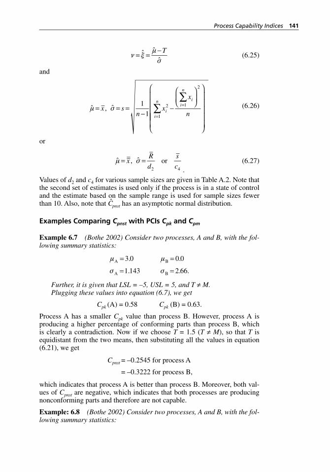
Process Capability Indices 141
ν ξ
µ
σ= =
−ˆ ˆˆ
T
(6.25)
and
ˆ , ˆµ σ= = =−
−
⎛
⎝⎜⎞
⎠⎟⎛
⎝
⎜⎜⎜
=
=
∑∑x s
nx
x
ni
ii
n
i
n1
12 1
2
1⎜⎜⎜
⎞
⎠
⎟⎟⎟⎟⎟
(6.26)
or
ˆ , ˆµ σ= =x
R
d
s
c2 4
or.
(6.27)
Values of d2 and c4 for various sample sizes are given in Table A.2. Note that the second set of estimates is used only if the process is in a state of control and the estimate based on the sample range is used for sample sizes fewer than 10. Also, note that Cpnst has an asymptotic normal distribution.
Examples Comparing Cpnst with PCIs Cpk and Cpm
Example 6.7 (Bothe 2002) Consider two processes, A and B, with the fol-lowing summary statistics:
µ µ
σ σ
A B
A B
= =
= =
3 0 0 0
1 143 2 66
. .
. . .
Further, it is given that LSL = –5, USL = 5, and T ≠ M.Plugging these values into equation (6.7), we get
Cpk (A) = 0.58 Cpk (B) = 0.63.
Process A has a smaller Cpk value than process B. However, process A is producing a higher percentage of conforming parts than process B, which is clearly a contradiction. Now if we choose T = 1.5 (T ≠ M), so that T is equidistant from the two means, then substituting all the values in equation (6.21), we get
Cpnst = –0.2545 for process A
= –0.3222 for process B,
which indicates that process A is better than process B. Moreover, both val-ues of Cpnst are negative, which indicates that both processes are producing nonconforming parts and therefore are not capable.
Example: 6.8 (Bothe 2002) Consider two processes, A and B, with the fol-lowing summary statistics:
H1277 ch06.indd 141H1277 ch06.indd 141 3/8/07 12:36:34 PM3/8/07 12:36:34 PM
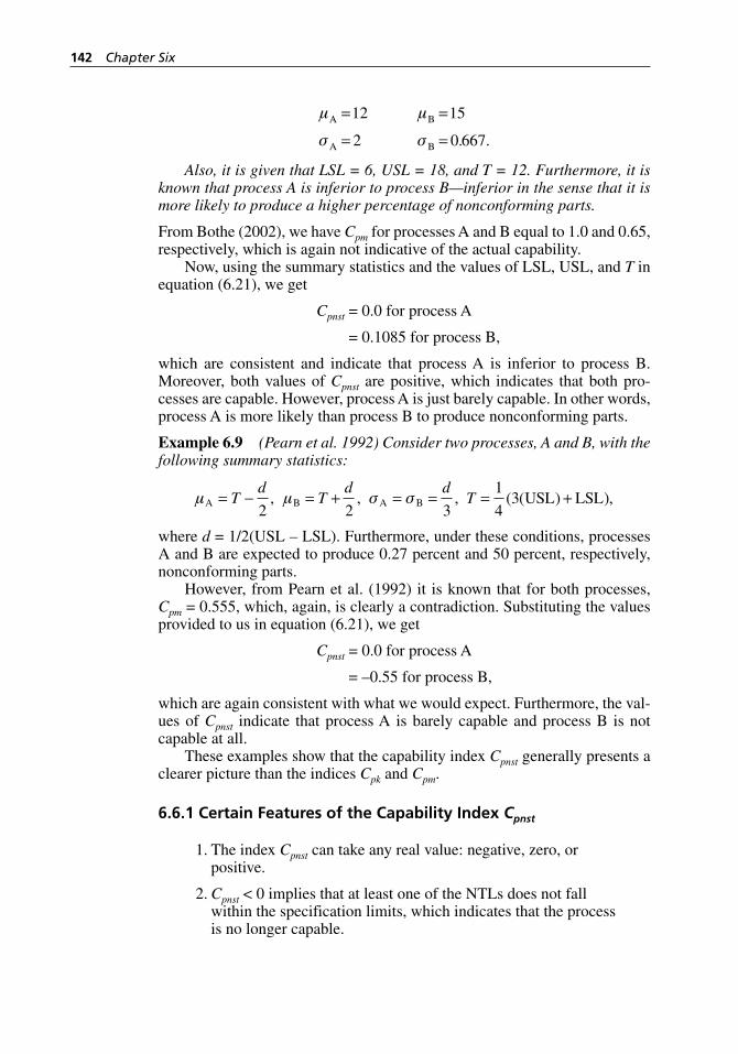
142 Chapter Six
µ µ
σ σ
A B
A B
= =
= =
12 15
2 0 667. .
Also, it is given that LSL = 6, USL = 18, and T = 12. Furthermore, it is known that process A is inferior to process B—inferior in the sense that it is more likely to produce a higher percentage of nonconforming parts.
From Bothe (2002), we have Cpm for processes A and B equal to 1.0 and 0.65, respectively, which is again not indicative of the actual capability.
Now, using the summary statistics and the values of LSL, USL, and T in equation (6.21), we get
Cpnst = 0.0 for process A
= 0.1085 for process B,
which are consistent and indicate that process A is inferior to process B. Moreover, both values of Cpnst are positive, which indicates that both pro-cesses are capable. However, process A is just barely capable. In other words, process A is more likely than process B to produce nonconforming parts.
Example 6.9 (Pearn et al. 1992) Consider two processes, A and B, with the following summary statistics:
µ µ σ σA B A B USL LSL= − = + = = = +T
dT
d dT
2 2 3
1
43, , , ( ( ) ),
where d = 1/2(USL – LSL). Furthermore, under these conditions, processes A and B are expected to produce 0.27 percent and 50 percent, respectively, nonconforming parts.
However, from Pearn et al. (1992) it is known that for both processes, Cpm = 0.555, which, again, is clearly a contradiction. Substituting the values provided to us in equation (6.21), we get
Cpnst = 0.0 for process A
= –0.55 for process B,
which are again consistent with what we would expect. Furthermore, the val-ues of Cpnst indicate that process A is barely capable and process B is not capable at all.
These examples show that the capability index Cpnst generally presents a clearer picture than the indices Cpk and Cpm.
6.6.1 Certain Features of the Capability Index Cpnst
1. The index Cpnst can take any real value: negative, zero, or positive.
2. Cpnst < 0 implies that at least one of the NTLs does not fall within the specification limits, which indicates that the process is no longer capable.
H1277 ch06.indd 142H1277 ch06.indd 142 3/8/07 12:36:35 PM3/8/07 12:36:35 PM
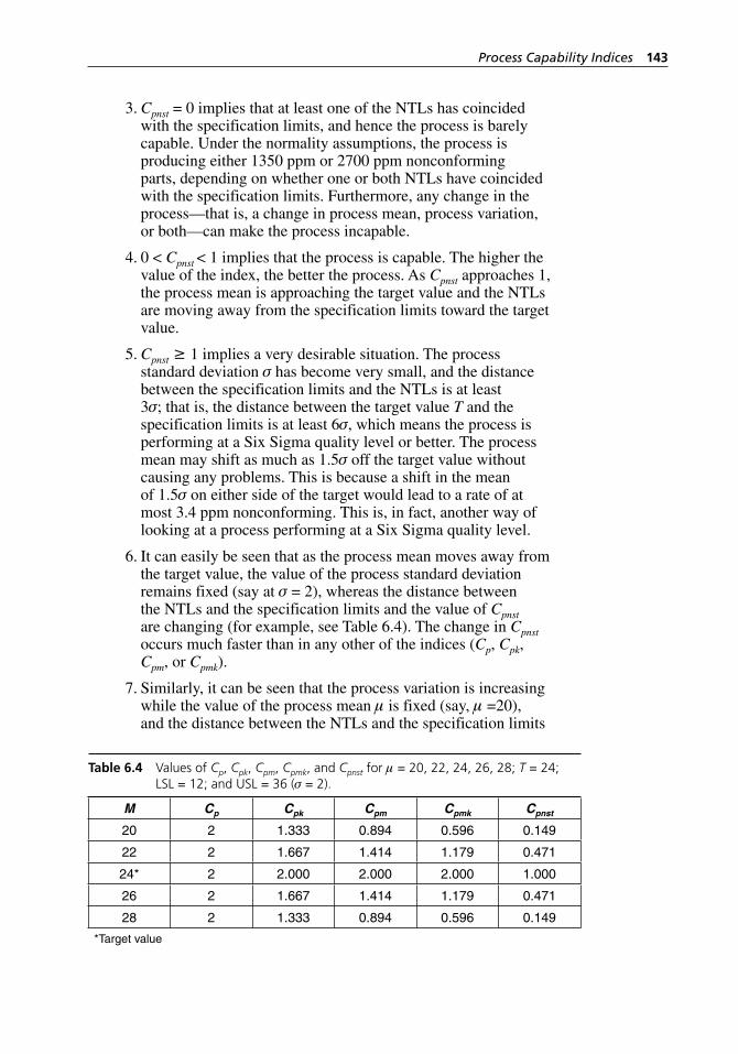
Process Capability Indices 143
3. Cpnst = 0 implies that at least one of the NTLs has coincided with the specification limits, and hence the process is barely capable. Under the normality assumptions, the process is producing either 1350 ppm or 2700 ppm nonconforming parts, depending on whether one or both NTLs have coincided with the specification limits. Furthermore, any change in the process—that is, a change in process mean, process variation, or both—can make the process incapable.
4. 0 < Cpnst < 1 implies that the process is capable. The higher the value of the index, the better the process. As Cpnst approaches 1, the process mean is approaching the target value and the NTLs are moving away from the specification limits toward the target value.
5. Cpnst ≥ 1 implies a very desirable situation. The process standard deviation σ has become very small, and the distance between the specification limits and the NTLs is at least 3σ; that is, the distance between the target value T and the specification limits is at least 6σ, which means the process is performing at a Six Sigma quality level or better. The process mean may shift as much as 1.5σ off the target value without causing any problems. This is because a shift in the mean of 1.5σ on either side of the target would lead to a rate of at most 3.4 ppm nonconforming. This is, in fact, another way of looking at a process performing at a Six Sigma quality level.
6. It can easily be seen that as the process mean moves away from the target value, the value of the process standard deviation remains fixed (say at σ = 2), whereas the distance between the NTLs and the specification limits and the value of Cpnst are changing (for example, see Table 6.4). The change in Cpnst occurs much faster than in any other of the indices (Cp, Cpk, Cpm, or Cpmk).
7. Similarly, it can be seen that the process variation is increasing while the value of the process mean µ is fixed (say, µ =20), and the distance between the NTLs and the specification limits
Table 6.4 Values of Cp, Cpk, Cpm, Cpmk, and Cpnst for µ = 20, 22, 24, 26, 28; T = 24; LSL = 12; and USL = 36 (σ = 2).
M Cp Cpk Cpm Cpmk Cpnst
20 2 1.333 0.894 0.596 0.149
22 2 1.667 1.414 1.179 0.471
24* 2 2.000 2.000 2.000 1.000
26 2 1.667 1.414 1.179 0.471
28 2 1.333 0.894 0.596 0.149
*Target value
H1277 ch06.indd 143H1277 ch06.indd 143 3/8/07 12:36:35 PM3/8/07 12:36:35 PM
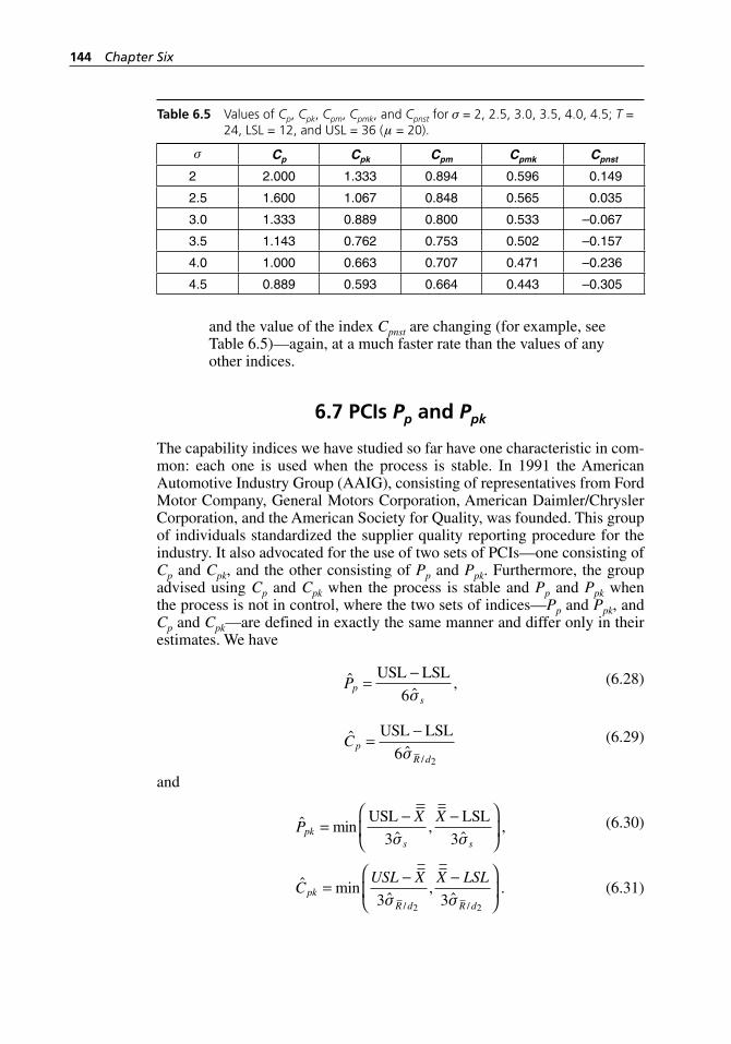
144 Chapter Six
and the value of the index Cpnst are changing (for example, see Table 6.5)—again, at a much faster rate than the values of any other indices.
6.7 PCIs Pp and Ppk
The capability indices we have studied so far have one characteristic in com-mon: each one is used when the process is stable. In 1991 the American Automotive Industry Group (AAIG), consisting of representatives from Ford Motor Company, General Motors Corporation, American Daimler/Chrysler Corporation, and the American Society for Quality, was founded. This group of individuals standardized the supplier quality reporting procedure for the industry. It also advocated for the use of two sets of PCIs—one consisting of Cp and Cpk, and the other consisting of Pp and Ppk. Furthermore, the group advised using Cp and Cpk when the process is stable and Pp and Ppk when the process is not in control, where the two sets of indices—Pp and Ppk, and Cp and Cpk—are defined in exactly the same manner and differ only in their estimates. We have
ˆ
ˆ,Pp
s
=−USL LSL
6σ (6.28)
ˆˆ
,/
CpR d
=−USL LSL
62
σ
(6.29)
and
ˆ minˆ
,ˆ
,PX X
pks s
=− −⎛
⎝⎜
⎞
⎠⎟
USL LSL
3 3σ σ
(6.30)
ˆ minˆ
,ˆ/ /
CUSL X X LSL
pkR d R d
=− −⎛
⎝⎜
⎞
⎠⎟3 3
2 2σ σ
.
(6.31)
Table 6.5 Values of Cp, Cpk, Cpm, Cpmk, and Cpnst for σ = 2, 2.5, 3.0, 3.5, 4.0, 4.5; T = 24, LSL = 12, and USL = 36 (µ = 20).
σ Cp Cpk Cpm Cpmk Cpnst
2 2.000 1.333 0.894 0.596 0.149
2.5 1.600 1.067 0.848 0.565 0.035
3.0 1.333 0.889 0.800 0.533 –0.067
3.5 1.143 0.762 0.753 0.502 –0.157
4.0 1.000 0.663 0.707 0.471 –0.236
4.5 0.889 0.593 0.664 0.443 –0.305
H1277 ch06.indd 144H1277 ch06.indd 144 3/8/07 12:36:35 PM3/8/07 12:36:35 PM
Process Capability Indices 145
In other words, they differ only in the method in which one estimates the standard deviation. The estimate σs is the usual standard deviation
s x x mnijj
m
i
n
= − −==
∑∑ ( ) / ( ),2
11
1 and ˆ //σ R d R d2 2= is an estimate obtained
using the subgroup ranges Ri, i = 1, 2, . . . , m and the corresponding value of d2. Note that the estimate σs measures the process variability by using the variability within and between subgroups, whereas ˆ
/σ R d2 uses only the vari-
ability within the subgroups. When the process is stable, there is very little variability between the subgroups; the two sets of indices are essentially the same because the estimates σs and ˆ /σ R d2
are approximately equal. But if the process is not stable, there is potentially a very large variability between the subgroups. This would mean that ˆ /σ R d2
underestimates the process standard deviation, and consequently Cpk would overestimate the process capability. Fortunately, this situation will not arise, because the use of Cpk is recom-mended only when the process is stable.
Kotz and Lovelace (1998, 253) strongly argue against the use of Pp and Ppk: “We highly recommend against using these indices when the process is not in statistical control. Under these conditions, the P-numbers are meaning-less with regard to process capability, have no tractable statistical properties, and infer nothing about long- term capability of the process. Worse still, they provide no motivation to the user- companies to get their process in control. The P-numbers are a step backwards in the efforts to properly quantify pro-cess capability, and a step towards statistical terrorism in its undiluted form.” Montgomery (2005b, 349) agrees with Kotz and Lovelace: “The process per-formance indices Pp and Ppk are more than a step backwards. They are a waste of engineering and management effort—they tell you nothing.” The authors wholeheartedly agree with Kotz and Lovelace and Montgomery. No one can judge a process when its future behavior is so unpredictable.
H1277 ch06.indd 145H1277 ch06.indd 145 3/8/07 12:36:35 PM3/8/07 12:36:35 PM

H1277 ch06.indd 146H1277 ch06.indd 146 3/8/07 12:36:35 PM3/8/07 12:36:35 PM
147
Measurement Systems Analysis (MSA) is used to understand and quantify the variability associated with measurements and mea-surement systems. In the Measurement Systems Analysis Reference
Manual, the Automotive Industry Action Group (AIAG) and MSA Work Group (2002, 64) define measurement and measurement systems as follows:
Definition 7.1 Measurement: “the assignment of numbers [or val-ues] to material things to represent the relations among them with respect to particular properties.”
Definition 7.2 Measurement system: “the collection of instruments or gauges, standards, operations, methods, fixtures, software, person-nel, environment and assumptions used to quantify a unit of measure or fix assessment to the feature characteristic being measured; the complete process used to obtain measurements.”
These definitions will serve as the basis of our discussion. However, we must first provide a clarification. The term MSA is commonly used interchange-ably with the term Gage repeatability and reproducibility (Gage R&R). MSA is a more comprehensive analysis quantifying variability components from gage stability, gage bias, gage linearity, and gage repeatability and reproduc-ibility (that is, variability from operator measurements). Gage R&R is, in fact, a subset or component of MSA. The underlying reason for mistaken interchange of the two terms is that many, if not most, problems with mea-surement systems are detected and corrected with the Gage R&R procedure without having to continue with a more comprehensive MSA. For a detailed discussion of analysis techniques for gage stability, gage bias, and gage lin-earity, see AIAG and MSA Work Group (2002).
7
Measurement Systems Analysis
H1277 ch07.indd 147H1277 ch07.indd 147 3/8/07 5:58:27 PM3/8/07 5:58:27 PM
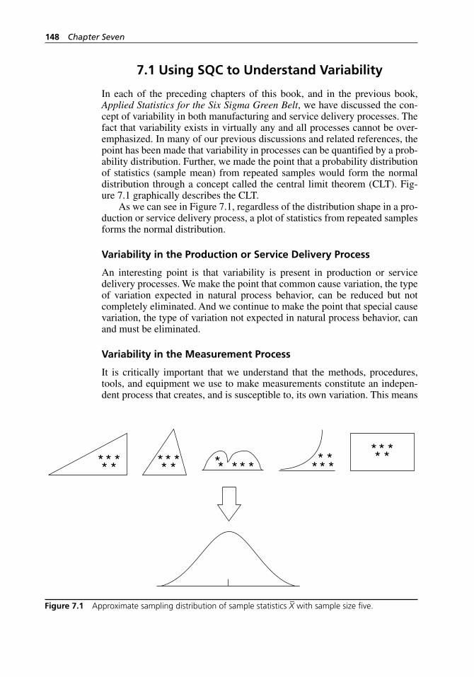
148 Chapter Seven
7.1 Using SQC to Understand Variability
In each of the preceding chapters of this book, and in the previous book, Applied Statistics for the Six Sigma Green Belt, we have discussed the con-cept of variability in both manufacturing and service delivery processes. The fact that variability exists in virtually any and all processes cannot be over-emphasized. In many of our previous discussions and related references, the point has been made that variability in processes can be quantified by a prob-ability distribution. Further, we made the point that a probability distribution of statistics (sample mean) from repeated samples would form the normal distribution through a concept called the central limit theorem (CLT). Fig-ure 7.1 graphically describes the CLT.
As we can see in Figure 7.1, regardless of the distribution shape in a pro-duction or service delivery process, a plot of statistics from repeated samples forms the normal distribution.
Variability in the Production or Service Delivery Process
An interesting point is that variability is present in production or service delivery processes. We make the point that common cause variation, the type of variation expected in natural process behavior, can be reduced but not completely eliminated. And we continue to make the point that special cause variation, the type of variation not expected in natural process behavior, can and must be eliminated.
Variability in the Measurement Process
It is critically important that we understand that the methods, procedures, tools, and equipment we use to make measurements constitute an indepen-dent process that creates, and is susceptible to, its own variation. This means
** ** * ** ** *** ** *
* ** * *** * * *
Figure 7.1 Approximate sampling distribution of sample statistics X– with sample size five.
H1277 ch07.indd 148H1277 ch07.indd 148 3/8/07 5:58:28 PM3/8/07 5:58:28 PM
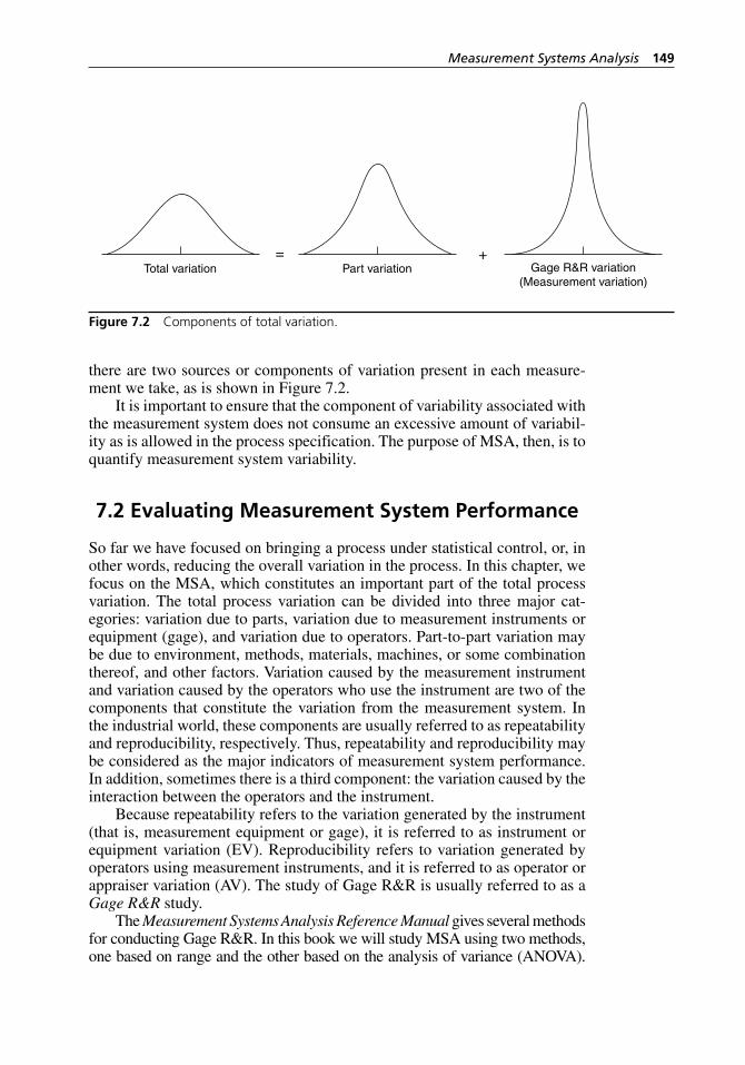
Measurement Systems Analysis 149
there are two sources or components of variation present in each measure-ment we take, as is shown in Figure 7.2.
It is important to ensure that the component of variability associated with the measurement system does not consume an excessive amount of variabil-ity as is allowed in the process specification. The purpose of MSA, then, is to quantify measurement system variability.
7.2 Evaluating Measurement System Performance
So far we have focused on bringing a process under statistical control, or, in other words, reducing the overall variation in the process. In this chapter, we focus on the MSA, which constitutes an important part of the total process variation. The total process variation can be divided into three major cat-egories: variation due to parts, variation due to measurement instruments or equipment (gage), and variation due to operators. Part- to-part variation may be due to environment, methods, materials, machines, or some combination thereof, and other factors. Variation caused by the measurement instrument and variation caused by the operators who use the instrument are two of the components that constitute the variation from the measurement system. In the industrial world, these components are usually referred to as repeatability and reproducibility, respectively. Thus, repeatability and reproducibility may be considered as the major indicators of measurement system performance. In addition, sometimes there is a third component: the variation caused by the interaction between the operators and the instrument.
Because repeatability refers to the variation generated by the instrument (that is, measurement equipment or gage), it is referred to as instrument or equipment variation (EV). Reproducibility refers to variation generated by operators using measurement instruments, and it is referred to as operator or appraiser variation (AV). The study of Gage R&R is usually referred to as a Gage R&R study.
The Measurement Systems Analysis Reference Manual gives several methods for conducting Gage R&R. In this book we will study MSA using two methods, one based on range and the other based on the analysis of variance (ANOVA).
= +Total variation Part variation Gage R&R variation
(Measurement variation)
Figure 7.2 Components of total variation.
H1277 ch07.indd 149H1277 ch07.indd 149 3/8/07 5:58:28 PM3/8/07 5:58:28 PM
150 Chapter Seven
Because ANOVA is an advanced statistical technique that is not covered in our first volume, Applied Statistics for the Six Sigma Green Belt, or in this book, details will be kept to a minimum. We will focus our attention on explaining and interpreting the results of an example that we will work out using computer software.
7.2.1 MSA Based on Range
Various authors, including IBM (1986) and Barrentine (2003), have presented a form of what is known as the range method. Before we discuss the details of this method, we will define certain terms, namely, measurement capability index, K1-Factor, and K2-Factor. In addition, we will define some other terms that are very useful in understanding the MSA.
An MSA is a technique for collecting and analyzing data to evaluate the effectiveness of the measurement process. To collect data, we randomly select some parts and then select a certain number of operators (usually three or more, but as a general rule, the more the better). Each operator takes mul-tiple measurements (at least two) on each part, and all the parts are measured in random order. These measurements are also known as trials. Using the terminology of the control charts discussed in earlier chapters, the measure-ments on each part (or the number of trials) constitute a rational subgroup, and the number of parts times the number of operators constitutes the num-ber of subgroups or samples. Then R
– is defined as the average of the ranges
of trials within the same operator, and –R– is defined as the average of the R
–’s
between the operators.
Definition 7.3 The measurement capability index (MCI) is a mea-surement that quantifies our belief that the gage is reliable enough to support decisions made under the existing circumstances.
The MCI relates to four characteristics of a measurement system, which are the key to any measurement system. These characteristics are:
1. Precision
2. Accuracy
3. Stability
4. Linearity
The characteristic precision is further subdivided into two categories: repeat-ability and reproducibility.
Definition 7.4 Repeatability measures the preciseness (consis-tency) of the observations taken under the same conditions, which is achieved by computing the variance of such observations.
H1277 ch07.indd 150H1277 ch07.indd 150 3/8/07 5:58:28 PM3/8/07 5:58:28 PM
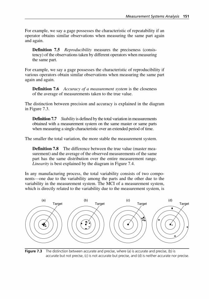
Measurement Systems Analysis 151
For example, we say a gage possesses the characteristic of repeatability if an operator obtains similar observations when measuring the same part again and again.
Definition 7.5 Reproducibility measures the preciseness (consis-tency) of the observations taken by different operators when measuring the same part.
For example, we say a gage possesses the characteristic of reproducibility if various operators obtain similar observations when measuring the same part again and again.
Definition 7.6 Accuracy of a measurement system is the closeness of the average of measurements taken to the true value.
The distinction between precision and accuracy is explained in the diagram in Figure 7.3.
Definition 7.7 Stability is defined by the total variation in measurements obtained with a measurement system on the same master or same parts when measuring a single characteristic over an extended period of time.
The smaller the total variation, the more stable the measurement system.
Definition 7.8 The difference between the true value (master mea-surement) and the average of the observed measurements of the same part has the same distribution over the entire measurement range. Linearity is best explained by the diagram in Figure 7.4.
In any manufacturing process, the total variability consists of two compo-nents—one due to the variability among the parts and the other due to the variability in the measurement system. The MCI of a measurement system, which is directly related to the variability due to the measurement system, is
(a) (b) (c) (d)Target Target Target Target
Figure 7.3 The distinction between accurate and precise, where (a) is accurate and precise, (b) is accurate but not precise, (c) is not accurate but precise, and (d) is neither accurate nor precise.
H1277 ch07.indd 151H1277 ch07.indd 151 3/8/07 5:58:28 PM3/8/07 5:58:28 PM
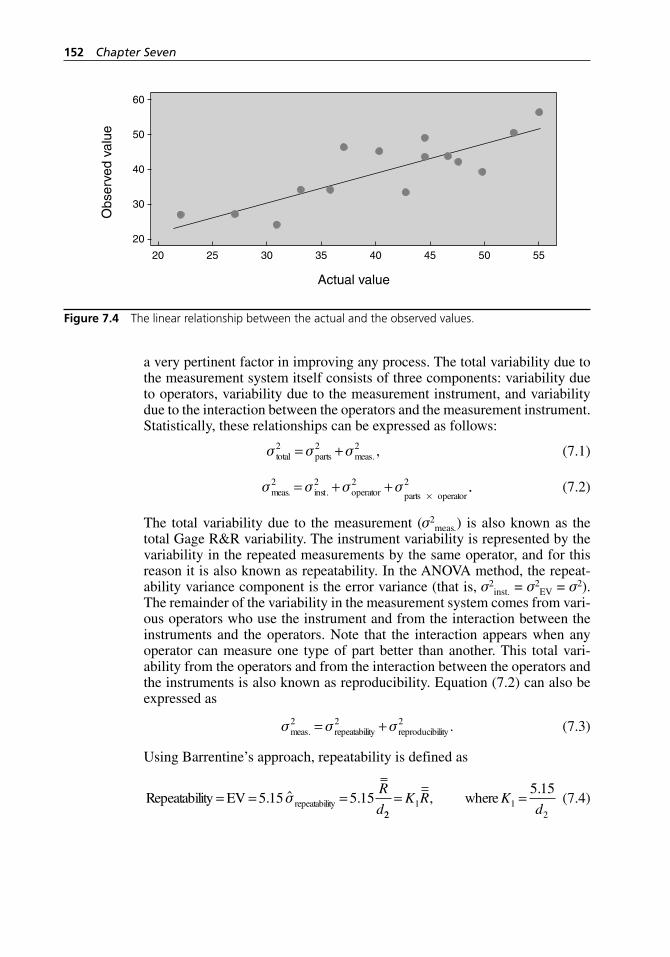
152 Chapter Seven
a very pertinent factor in improving any process. The total variability due to the measurement system itself consists of three components: variability due to operators, variability due to the measurement instrument, and variability due to the interaction between the operators and the measurement instrument. Statistically, these relationships can be expressed as follows:
σ σ σtotal parts meas
2 2 2= + . , (7.1)
σ σ σ σmeas. inst operator parts operator
2 2 2 2= + +×. ..
(7.2)
The total variability due to the measurement (σ2meas.) is also known as the
total Gage R&R variability. The instrument variability is represented by the variability in the repeated measurements by the same operator, and for this reason it is also known as repeatability. In the ANOVA method, the repeat-ability variance component is the error variance (that is, σ2
inst. = σ2EV = σ2).
The remainder of the variability in the measurement system comes from vari-ous operators who use the instrument and from the interaction between the instruments and the operators. Note that the interaction appears when any operator can measure one type of part better than another. This total vari-ability from the operators and from the interaction between the operators and the instruments is also known as reproducibility. Equation (7.2) can also be expressed as
σ σ σmeas repeatability reproducibility. .2 2 2= +
(7.3)
Using Barrentine’s approach, repeatability is defined as
Repeatability EV repeatability= = =5 15 5 15. ˆ .σR
d221 1
2
5 15= =K R K
d,
.where
(7.4)
20
30
40
50
60
5550454035302520
Actual value
Obs
erve
d va
lue
Figure 7.4 The linear relationship between the actual and the observed values.
H1277 ch07.indd 152H1277 ch07.indd 152 3/8/07 5:58:28 PM3/8/07 5:58:28 PM
Measurement Systems Analysis 153
and where the factor 5.15 represents the 99 percent range of the standard normal distribution, which follows from the fact that
P(–2.575 ≤ Z ≤ 2.575) = 0.99. (7.5)
Note that the AIAG recommends using the factor 6 instead of 5.15 because it covers almost 100 percent—or to be exact, 99.74 percent—of the range. Val-ues of K1 for various sample sizes (that is, the number of trials or the number of measurements taken on the same part by the same operator) are given in Table A.3. Duncan (1986) points out that this estimation procedure should be slightly modified if N = r × n = (# operators) × (# parts) is less than 16. If N is less than 16, then K1 is defined as
K
d1
2
5 15=
..
*
(7.6)
The values of d2* are listed in Duncan (1986), Table D3. The values of K1
listed in Table A.3 are determined according to the value of N. Again, using Barrentine’s notation (2003, 57), the Reproducibility = AV, ignoring the inter-action term, is defined as
Reproducibility AV
EV= = −
×( )
( )
( ),K R
r nx22
2
(7.7)
where r is the number of trials, n is the number of parts or samples, EV is as given in equation (7.4), Rx is the range of the operator’s means, and the factor K2 is defined as
K
d2
2
5 15=
..
*
(7.8)
The value of d2* can be found from Duncan’s Table D3 by selecting g = 1
and m = n (# operators). For example, if we have five operators, then from Duncan’s Table D3 for g = 1, m = 5, we have
K2
5 15
2 482 077= =
.
.. .
We now illustrate the range-based method and then the ANOVA method with the following example.
Example 7.1 A manufacturer of bolts (parts) used in automotive applica-tions has installed a new measuring gage. In order to perform the MSA on the new gage, the quality manager randomly selects three Six Sigma Green Belts from the quality control department, who decide to conduct the MSA by taking a random sample of 10 bolts. Each Six Sigma Green Belt takes three measurements on each bolt, which is randomly selected. The data obtained are as shown in Table 7.1.
H1277 ch07.indd 153H1277 ch07.indd 153 3/8/07 5:58:28 PM3/8/07 5:58:28 PM
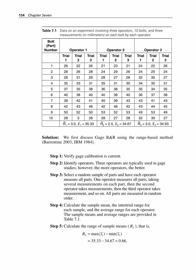
154 Chapter Seven
Table 7.1 Data on an experiment involving three operators, 10 bolts, and three measurements (in millimeters) on each bolt by each operator.
Bolt (Part)
Number Operator 1 Operator 2 Operator 3
Trial 1
Trial 2
Trial 3
Trial 1
Trial 2
Trial 3
Trial 1
Trial 2
Trial 3
1 26 22 26 21 23 21 24 22 26
2 28 26 28 24 29 26 24 25 24
3 28 31 28 28 27 28 32 30 27
4 35 33 31 35 31 30 34 35 31
5 37 35 38 36 38 35 35 34 35
6 40 38 40 40 38 40 36 37 38
7 39 42 41 40 39 43 43 41 43
8 42 43 46 42 46 42 43 44 45
9 50 52 50 53 52 53 49 53 49
10 28 3 28 28 27 28 32 30 27
R–
1 = 3.0, x–1 = 35.33 R–
2 = 2.5, x–2 = 34.67 R–
3 = 3.0, x–3 = 34.93
Solution: We first discuss Gage R&R using the range-based method (Barrentine 2003, IBM 1984).
Step 1: Verify gage calibration is current.
Step 2: Identify operators. Three operators are typically used in gage studies; however, the more operators, the better.
Step 3: Select a random sample of parts and have each operator measure all parts. One operator measures all parts, taking several measurements on each part, then the second operator takes measurements, then the third operator takes measurement, and so on. All parts are measured in random order.
Step 4: Calculate the sample mean, the intertrial range for each sample, and the average range for each operator. The sample means and average ranges are provided in Table 7.1.
Step 5: Calculate the range of sample means ( Rx ), that is,
R x xx i i= −
= − =
max min( ) ( )
. . . .35 33 34 67 0 66
H1277 ch07.indd 154H1277 ch07.indd 154 3/8/07 5:58:29 PM3/8/07 5:58:29 PM
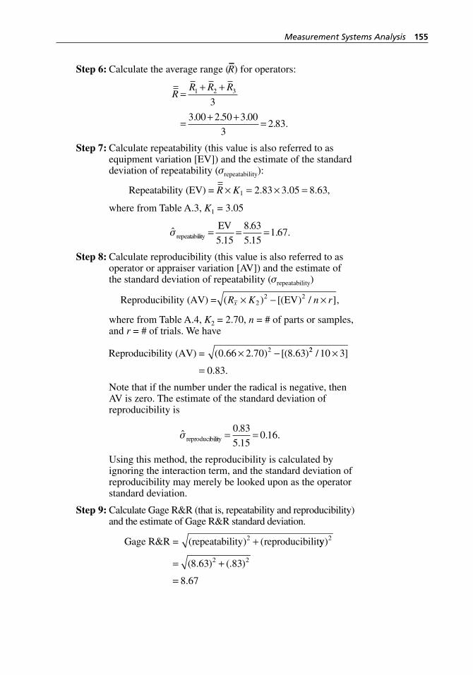
Measurement Systems Analysis 155
Step 6: Calculate the average range (–R–) for operators:
RR R R
=+ +
=+ +
=
1 2 3
3
3 00 2 50 3 00
32 83
. . .. .
Step 7: Calculate repeatability (this value is also referred to as equipment variation [EV]) and the estimate of the standard deviation of repeatability (σrepeatability):
Repeatability (EV) = R K× = × =1 2 83 3 05 8 63. . . ,
where from Table A.3, K1 = 3.05
ˆ
.
.
.. .σ repeatability
EV= = =
5 15
8 63
5 151 67
Step 8: Calculate reproducibility (this value is also referred to as operator or appraiser variation [AV]) and the estimate of the standard deviation of repeatability (σrepeatability)
Reproducibility (AV) = EV( ) [( ) / ],R K n rx × − ×22 2
where from Table A.4, K2 = 2.70, n = # of parts or samples, and r = # of trials. We have
Reproducibility (AV) = ( . . ) [( . )0 66 2 70 8 632× − 22 10 3
0 83
/ ]
. .
×
=Note that if the number under the radical is negative, then AV is zero. The estimate of the standard deviation of reproducibility is
ˆ .
.. .σ reproducibility = =
0 83
5 150 16
Using this method, the reproducibility is calculated by ignoring the interaction term, and the standard deviation of reproducibility may merely be looked upon as the operator standard deviation.
Step 9: Calculate Gage R&R (that is, repeatability and reproducibility) and the estimate of Gage R&R standard deviation.
Gage R&R = repeatability reproducibilit( ) (2 + yy)
( . ) (. )
.
2
2 28 63 83
8 67
= +
=
H1277 ch07.indd 155H1277 ch07.indd 155 3/8/07 5:58:29 PM3/8/07 5:58:29 PM
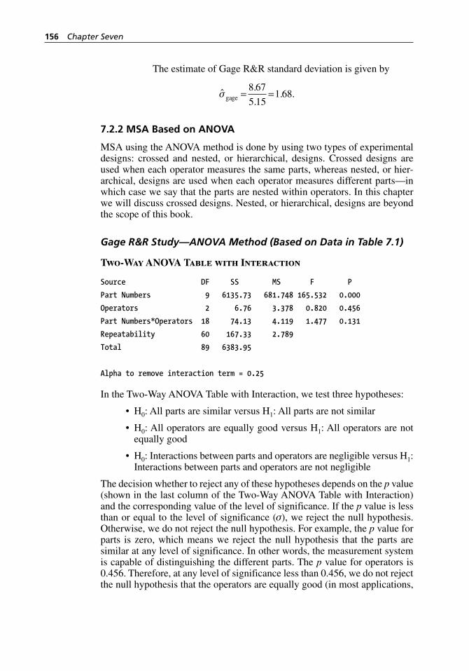
156 Chapter Seven
The estimate of Gage R&R standard deviation is given by
ˆ .
.. .σgage = =
8 67
5 151 68
7.2.2 MSA Based on ANOVA
MSA using the ANOVA method is done by using two types of experimental designs: crossed and nested, or hierarchical, designs. Crossed designs are used when each operator measures the same parts, whereas nested, or hier-archical, designs are used when each operator measures different parts—in which case we say that the parts are nested within operators. In this chapter we will discuss crossed designs. Nested, or hierarchical, designs are beyond the scope of this book.
Gage R&R Study—ANOVA Method (Based on Data in Table 7.1)
Two-Way ANOVA Table with Interaction
Source DF SS MS F P
Part Numbers 9 6135.73 681.748 165.532 0.000
Operators 2 6.76 3.378 0.820 0.456
Part Numbers*Operators 18 74.13 4.119 1.477 0.131
Repeatability 60 167.33 2.789
Total 89 6383.95
Alpha to remove interaction term = 0.25
In the Two- Way ANOVA Table with Interaction, we test three hypotheses:
H0: All parts are similar versus H1: All parts are not similar
H0: All operators are equally good versus H1: All operators are not equally good
H0: Interactions between parts and operators are negligible versus H1: Interactions between parts and operators are not negligible
The decision whether to reject any of these hypotheses depends on the p value (shown in the last column of the Two- Way ANOVA Table with Interaction) and the corresponding value of the level of significance. If the p value is less than or equal to the level of significance (σ), we reject the null hypothesis. Otherwise, we do not reject the null hypothesis. For example, the p value for parts is zero, which means we reject the null hypothesis that the parts are similar at any level of significance. In other words, the measurement system is capable of distinguishing the different parts. The p value for operators is 0.456. Therefore, at any level of significance less than 0.456, we do not reject the null hypothesis that the operators are equally good (in most applications,
•
•
•
H1277 ch07.indd 156H1277 ch07.indd 156 3/8/07 5:58:29 PM3/8/07 5:58:29 PM
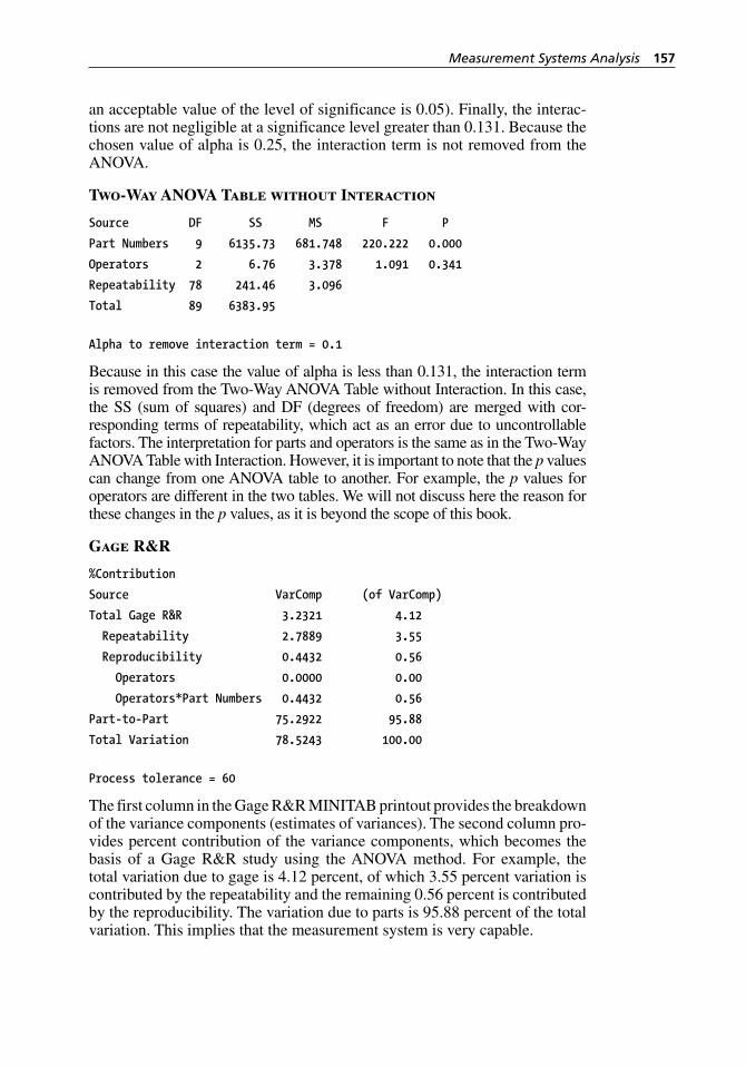
Measurement Systems Analysis 157
an acceptable value of the level of significance is 0.05). Finally, the interac-tions are not negligible at a significance level greater than 0.131. Because the chosen value of alpha is 0.25, the interaction term is not removed from the ANOVA.
Two-Way ANOVA Table without Interaction
Source DF SS MS F P
Part Numbers 9 6135.73 681.748 220.222 0.000
Operators 2 6.76 3.378 1.091 0.341
Repeatability 78 241.46 3.096
Total 89 6383.95
Alpha to remove interaction term = 0.1
Because in this case the value of alpha is less than 0.131, the interaction term is removed from the Two- Way ANOVA Table without Interaction. In this case, the SS (sum of squares) and DF (degrees of freedom) are merged with cor-responding terms of repeatability, which act as an error due to uncontrollable factors. The interpretation for parts and operators is the same as in the Two- Way ANOVA Table with Interaction. However, it is important to note that the p values can change from one ANOVA table to another. For example, the p values for operators are different in the two tables. We will not discuss here the reason for these changes in the p values, as it is beyond the scope of this book.
Gage R&R
%Contribution
Source VarComp (of VarComp)
Total Gage R&R 3.2321 4.12
Repeatability 2.7889 3.55
Reproducibility 0.4432 0.56
Operators 0.0000 0.00
Operators*Part Numbers 0.4432 0.56
Part-to-Part 75.2922 95.88
Total Variation 78.5243 100.00
Process tolerance = 60
The first column in the Gage R&R MINITAB printout provides the breakdown of the variance components (estimates of variances). The second column pro-vides percent contribution of the variance components, which becomes the basis of a Gage R&R study using the ANOVA method. For example, the total variation due to gage is 4.12 percent, of which 3.55 percent variation is contributed by the repeatability and the remaining 0.56 percent is contributed by the reproducibility. The variation due to parts is 95.88 percent of the total variation. This implies that the measurement system is very capable.
H1277 ch07.indd 157H1277 ch07.indd 157 3/8/07 5:58:29 PM3/8/07 5:58:29 PM
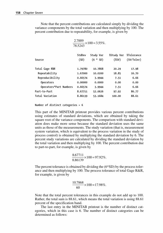
158 Chapter Seven
Note that the percent contributions are calculated simply by dividing the variance components by the total variation and then multiplying by 100. The percent contribution due to repeatability, for example, is given by
2 7889
78 5243100 3 55
.
.. %.× =
StdDev Study Var %Study Var %Tolerance
Source (SD) (6 * SD) (%SV) (SV/Toler)
Total Gage R&R 1.79780 10.7868 20.29 17.98
Repeatability 1.67000 10.0200 18.85 16.70
Reproducibility 0.66574 3.9944 7.51 6.66
Operators 0.00000 0.0000 0.00 0.00
Operators*Part Numbers 0.66574 3.9944 7.51 6.66
Part-to-Part 8.67711 52.0626 97.92 86.77
Total Variation 8.86139 53.1684 100.00 88.61
Number of distinct categories = 6
This part of the MINITAB printout provides various percent contributions using estimates of standard deviations, which are obtained by taking the square root of the variance components. The comparison with standard devi-ation does make more sense because the standard deviation uses the same units as those of the measurements. The study variation (that is, measurement system variation, which is equivalent to the process variation in the study of process control) is obtained by multiplying the standard deviation by 6. The percent study variations are calculated by dividing the standard deviation by the total variation and then multiplying by 100. The percent contribution due to part- to-part, for example, is given by
8 67711
8 86139100 97 92
.
.. %.× =
The percent tolerance is obtained by dividing the (6*SD) by the process toler-ance and then multiplying by 100. The process tolerance of total Gage R&R, for example, is given by
10 7868
60100 17 98
.. %.× =
Note that the total percent tolerances in this example do not add up to 100. Rather, the total sum is 88.61, which means the total variation is using 88.61 percent of the specification band.
The last entry in the MINITAB printout is the number of distinct cat-egories, which in this case is 6. The number of distinct categories can be determined as follows:
H1277 ch07.indd 158H1277 ch07.indd 158 3/8/07 5:58:29 PM3/8/07 5:58:29 PM
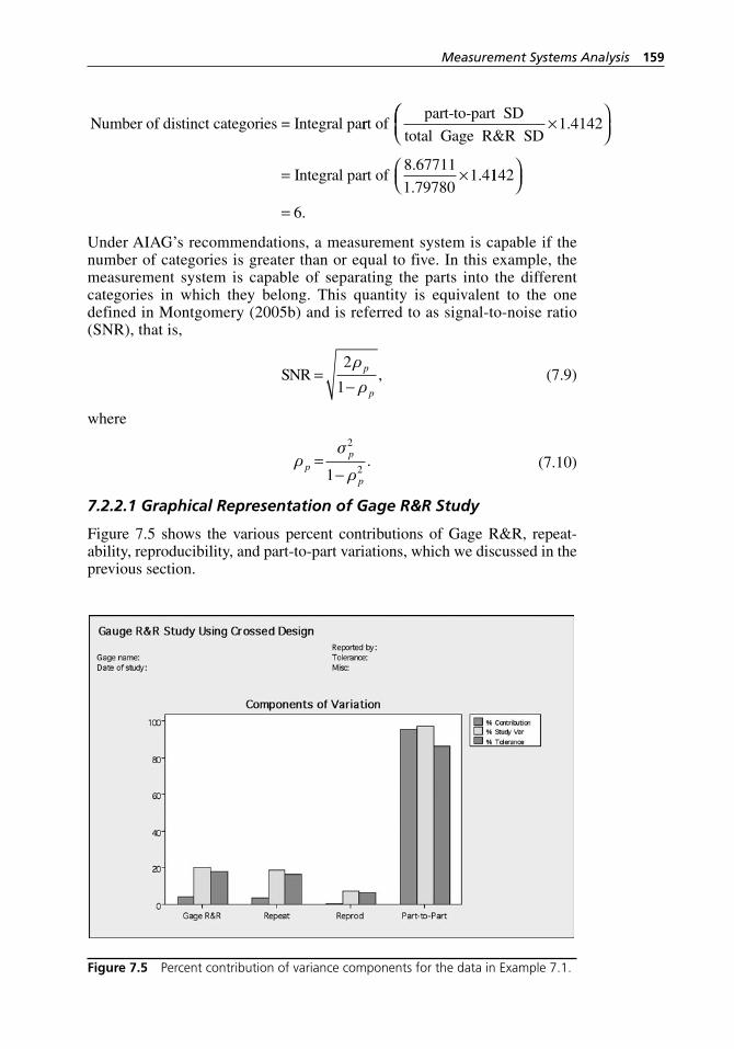
Measurement Systems Analysis 159
Number of distinct categories = Integral parrt ofpart-to-part SD
total Gage R&R SD×1 4142.
⎛⎛⎝⎜
⎞⎠⎟
= ×Integral part of8 67711
1 797801 4
.
.. 1142
6
⎛⎝⎜
⎞⎠⎟
= .
Under AIAG’s recommendations, a measurement system is capable if the number of categories is greater than or equal to five. In this example, the measurement system is capable of separating the parts into the different categories in which they belong. This quantity is equivalent to the one defined in Montgomery (2005b) and is referred to as signal- to-noise ratio (SNR), that is,
SNR =−2
1
ρ
ρp
p
,
(7.9)
where
ρσ
ρp
p
p
=−
2
21.
(7.10)
7.2.2.1 Graphical Representation of Gage R&R Study
Figure 7.5 shows the various percent contributions of Gage R&R, repeat-ability, reproducibility, and part- to-part variations, which we discussed in the previous section.
Figure 7.5 Percent contribution of variance components for the data in Example 7.1.
H1277 ch07.indd 159H1277 ch07.indd 159 3/8/07 5:58:29 PM3/8/07 5:58:29 PM
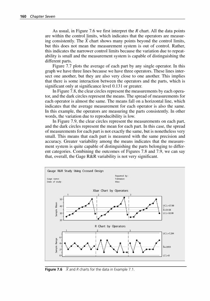
160 Chapter Seven
As usual, in Figure 7.6 we first interpret the R chart. All the data points are within the control limits, which indicates that the operators are measur-ing consistently. The X
– chart shows many points beyond the control limits,
but this does not mean the measurement system is out of control. Rather, this indicates the narrower control limits because the variation due to repeat-ability is small and the measurement system is capable of distinguishing the different parts.
Figure 7.7 plots the average of each part by any single operator. In this graph we have three lines because we have three operators. These lines inter-sect one another, but they are also very close to one another. This implies that there is some interaction between the operators and the parts, which is significant only at significance level 0.131 or greater.
In Figure 7.8, the clear circles represent the measurements by each opera-tor, and the dark circles represent the means. The spread of measurements for each operator is almost the same. The means fall on a horizontal line, which indicates that the average measurement for each operator is also the same. In this example, the operators are measuring the parts consistently. In other words, the variation due to reproducibility is low.
In Figure 7.9, the clear circles represent the measurements on each part, and the dark circles represent the mean for each part. In this case, the spread of measurements for each part is not exactly the same, but is nonetheless very small. This means that each part is measured with the same precision and accuracy. Greater variability among the means indicates that the measure-ment system is quite capable of distinguishing the parts belonging to differ-ent categories. Combining the outcomes of Figures 7.8 and 7.9, we can say that, overall, the Gage R&R variability is not very significant.
Figure 7.6 X– and R charts for the data in Example 7.1.
H1277 ch07.indd 160H1277 ch07.indd 160 3/8/07 5:58:30 PM3/8/07 5:58:30 PM
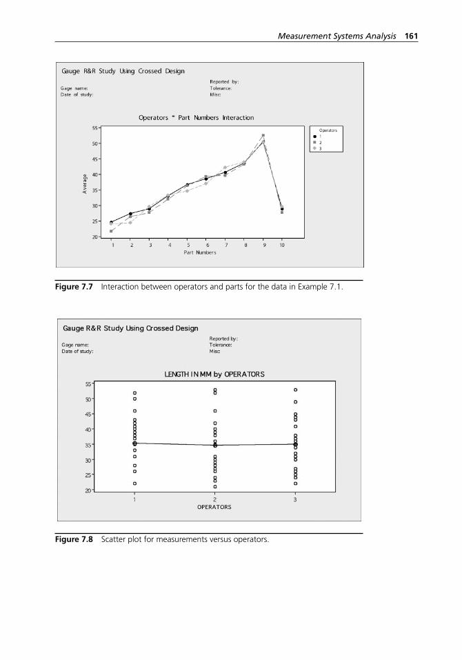
Measurement Systems Analysis 161
Figure 7.7 Interaction between operators and parts for the data in Example 7.1.
Figure 7.8 Scatter plot for measurements versus operators.
H1277 ch07.indd 161H1277 ch07.indd 161 3/8/07 5:58:30 PM3/8/07 5:58:30 PM
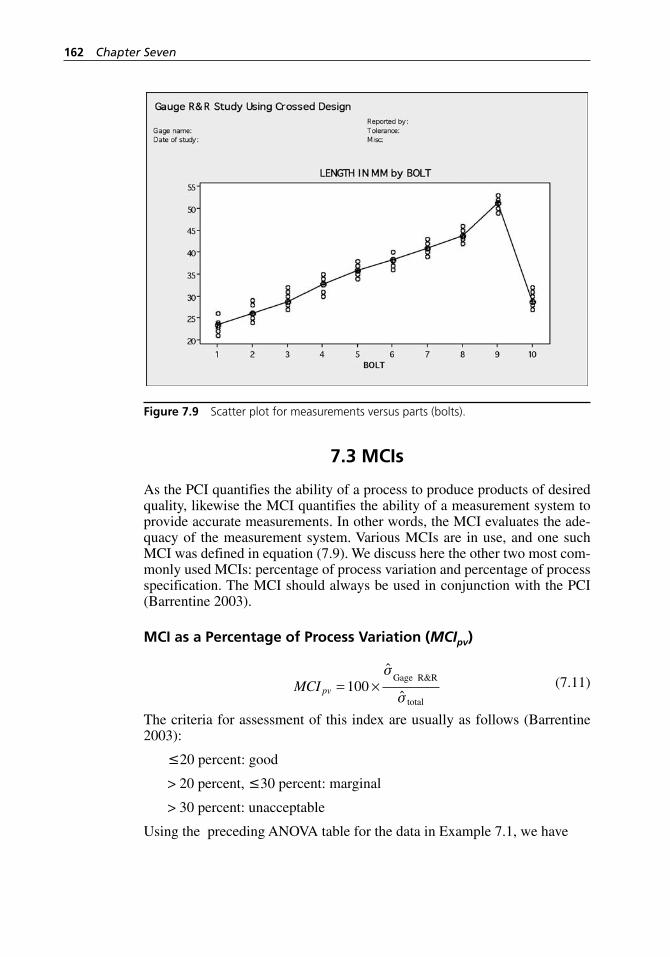
162 Chapter Seven
7.3 MCIs
As the PCI quantifies the ability of a process to produce products of desired quality, likewise the MCI quantifies the ability of a measurement system to provide accurate measurements. In other words, the MCI evaluates the ade-quacy of the measurement system. Various MCIs are in use, and one such MCI was defined in equation (7.9). We discuss here the other two most com-monly used MCIs: percentage of process variation and percentage of process specification. The MCI should always be used in conjunction with the PCI (Barrentine 2003).
MCI as a Percentage of Process Variation (MCIpv)
MCI pv = ×100
ˆ
ˆ
σ
σ
Gage R&R
total (7.11)
The criteria for assessment of this index are usually as follows (Barrentine 2003):
≤20 percent: good
> 20 percent, ≤30 percent: marginal
> 30 percent: unacceptable
Using the preceding ANOVA table for the data in Example 7.1, we have
Figure 7.9 Scatter plot for measurements versus parts (bolts).
H1277 ch07.indd 162H1277 ch07.indd 162 3/8/07 5:58:30 PM3/8/07 5:58:30 PM
Measurement Systems Analysis 163
MCI pv = × =100
1 79780
8 8613920
.
.%.
This MCI indicates that the measurement system is good.
MCI as a Percentage of Process Specification (MCIps)
MCI ps =
×
−
6 σGage R&R
USL LSL (7.12)
The criteria for assessment of this index are the same as MCIpv (Barrentine 2003):
≤20 percent: good
> 20 percent, ≤30 percent: marginal
> 30 percent: unacceptable
Again, using the preceding ANOVA table for the data in Example 7.1 and with process tolerance 60, we have
MCI ps = ×
×=100
6 1 79780
6018
.%.
Thus, this MCI indicates that the measurement system is good.
H1277 ch07.indd 163H1277 ch07.indd 163 3/8/07 5:58:31 PM3/8/07 5:58:31 PM

H1277 ch07.indd 164H1277 ch07.indd 164 3/8/07 5:58:31 PM3/8/07 5:58:31 PM
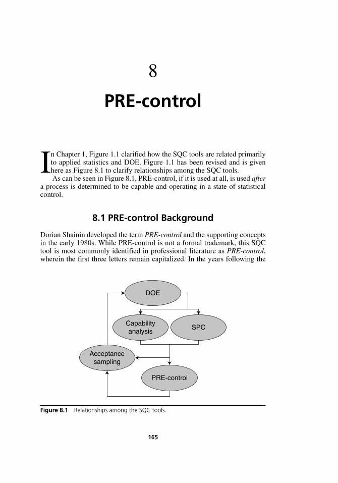
165
In Chapter 1, Figure 1.1 clarified how the SQC tools are related primarily to applied statistics and DOE. Figure 1.1 has been revised and is given here as Figure 8.1 to clarify relationships among the SQC tools.As can be seen in Figure 8.1, PRE- control, if it is used at all, is used after
a process is determined to be capable and operating in a state of statistical control.
8.1 PRE- control Background
Dorian Shainin developed the term PRE-control and the supporting concepts in the early 1980s. While PRE- control is not a formal trademark, this SQC tool is most commonly identified in professional literature as PRE-control, wherein the first three letters remain capitalized. In the years following the
8
PRE-control
SPCCapabilityanalysis
PRE-control
Acceptancesampling
DOE
Figure 8.1 Relationships among the SQC tools.
H1277 ch08.indd 165H1277 ch08.indd 165 3/8/07 12:37:39 PM3/8/07 12:37:39 PM
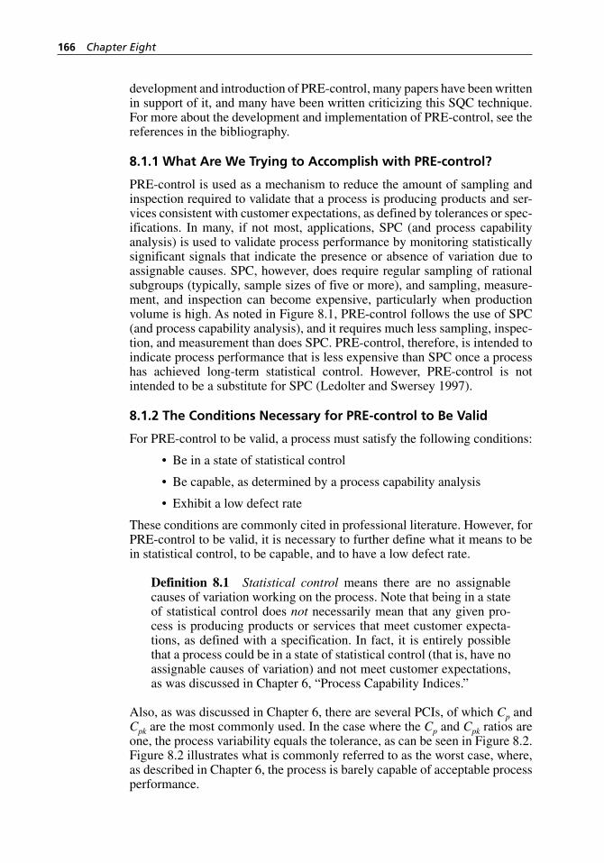
166 Chapter Eight
development and introduction of PRE- control, many papers have been written in support of it, and many have been written criticizing this SQC technique. For more about the development and implementation of PRE- control, see the references in the bibliography.
8.1.1 What Are We Trying to Accomplish with PRE- control?
PRE-control is used as a mechanism to reduce the amount of sampling and inspection required to validate that a process is producing products and ser-vices consistent with customer expectations, as defined by tolerances or spec-ifications. In many, if not most, applications, SPC (and process capability analysis) is used to validate process performance by monitoring statistically significant signals that indicate the presence or absence of variation due to assignable causes. SPC, however, does require regular sampling of rational subgroups (typically, sample sizes of five or more), and sampling, measure-ment, and inspection can become expensive, particularly when production volume is high. As noted in Figure 8.1, PRE- control follows the use of SPC (and process capability analysis), and it requires much less sampling, inspec-tion, and measurement than does SPC. PRE- control, therefore, is intended to indicate process performance that is less expensive than SPC once a process has achieved long- term statistical control. However, PRE- control is not intended to be a substitute for SPC (Ledolter and Swersey 1997).
8.1.2 The Conditions Necessary for PRE- control to Be Valid
For PRE- control to be valid, a process must satisfy the following conditions:
Be in a state of statistical control
Be capable, as determined by a process capability analysis
Exhibit a low defect rate
These conditions are commonly cited in professional literature. However, for PRE- control to be valid, it is necessary to further define what it means to be in statistical control, to be capable, and to have a low defect rate.
Definition 8.1 Statistical control means there are no assignable causes of variation working on the process. Note that being in a state of statistical control does not necessarily mean that any given pro-cess is producing products or services that meet customer expecta-tions, as defined with a specification. In fact, it is entirely possible that a process could be in a state of statistical control (that is, have no assignable causes of variation) and not meet customer expectations, as was discussed in Chapter 6, “Process Capability Indices.”
Also, as was discussed in Chapter 6, there are several PCIs, of which Cp and Cpk are the most commonly used. In the case where the Cp and Cpk ratios are one, the process variability equals the tolerance, as can be seen in Figure 8.2. Figure 8.2 illustrates what is commonly referred to as the worst case, where, as described in Chapter 6, the process is barely capable of acceptable process performance.
•
•
•
H1277 ch08.indd 166H1277 ch08.indd 166 3/8/07 12:37:40 PM3/8/07 12:37:40 PM
PRE-control 167
We see in Figure 8.2 that any process drift or shift will result in the pro-duction of products or services outside customer specifications or tolerances. So for PRE- control to be a valid SQC tool, the process capability ratio must be something greater than one, which means there is some room for the pro-cess to vary and yet still produce products or services that meet customer expectations. How high the PCI Cpk should be to make PRE- control valid is commonly defined in professional literature as 1.5, which equates to six stan-dard deviations of variability consuming only 0.88 of the tolerance. Process capability ratios at or above two are commonly considered to be economi-cally unjustified. And because PRE- control is valid only on processes with capability ratios at or above 1.5, and processes with capability ratios above 2 are not particularly common, PRE- control has a fairly limited range of use.
Lastly, what constitutes a low defect rate as a condition validating the use of PRE- control is a matter of debate. There are no guidelines, heuristics, or rules of thumb to qualify a process as having a low defect rate. Several publi-cations cited in the bibliography identify the term “near zero” defect rate to describe the conditions necessary to validate the use of PRE- control. It is clear that whatever value is selected for a low defect rate standard, the process must be inherently stable and capable, and it must have been through enough itera-tions of process improvement that defects are extremely unlikely to occur.
8.2 Global Perspective on the Use of PRE- control (Understanding the Color- Coding Scheme)
PRE-control uses a color- coding scheme associated with each of six zones consistent with Figure 8.3.
Figure 8.3 shows two green zones (some authors consider there to be only one large green zone), two yellow zones, and two red zones. Because PRE- control is based on the standard normal distribution, which is a symmetrical distribution, there is one green, one yellow, and one red zone on each side of the process target (center). Whether or not intended by the originator of
LNTLLSL USL
UNTLTarget
Figure 8.2 A barely capable process.
H1277 ch08.indd 167H1277 ch08.indd 167 3/8/07 12:37:40 PM3/8/07 12:37:40 PM
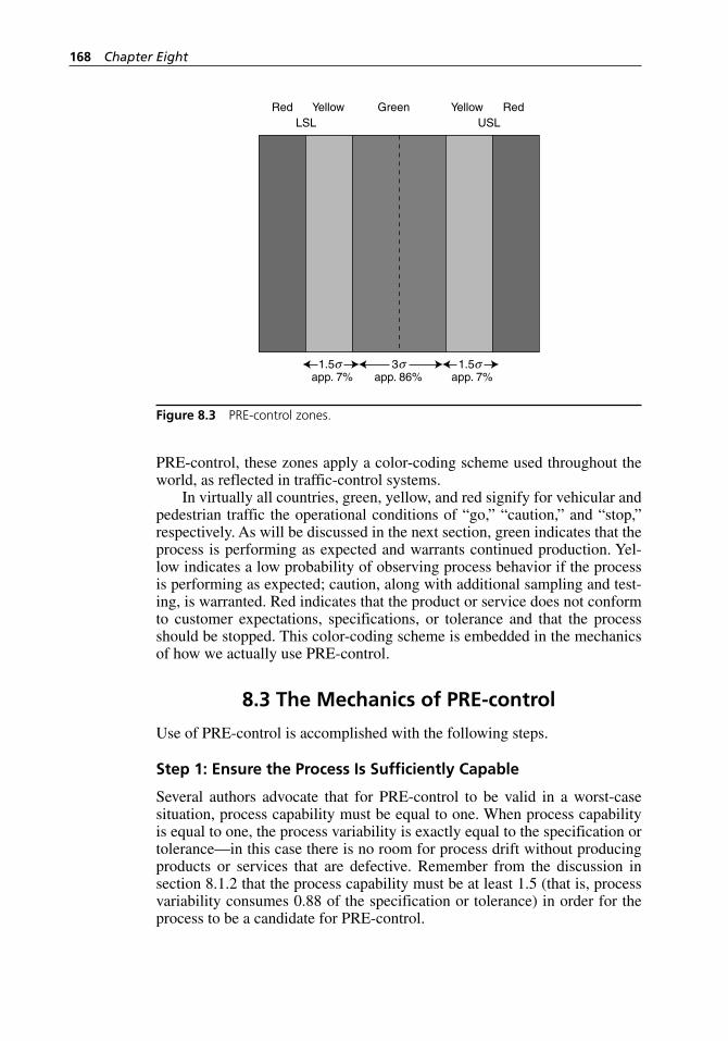
168 Chapter Eight
PRE-control, these zones apply a color- coding scheme used throughout the world, as reflected in traffic- control systems.
In virtually all countries, green, yellow, and red signify for vehicular and pedestrian traffic the operational conditions of “go,” “caution,” and “stop,” respectively. As will be discussed in the next section, green indicates that the process is performing as expected and warrants continued production. Yel-low indicates a low probability of observing process behavior if the process is performing as expected; caution, along with additional sampling and test-ing, is warranted. Red indicates that the product or service does not conform to customer expectations, specifications, or tolerance and that the process should be stopped. This color- coding scheme is embedded in the mechanics of how we actually use PRE- control.
8.3 The Mechanics of PRE- control
Use of PRE- control is accomplished with the following steps.
Step 1: Ensure the Process Is Sufficiently Capable
Several authors advocate that for PRE- control to be valid in a worst- case situation, process capability must be equal to one. When process capability is equal to one, the process variability is exactly equal to the specification or tolerance—in this case there is no room for process drift without producing products or services that are defective. Remember from the discussion in section 8.1.2 that the process capability must be at least 1.5 (that is, process variability consumes 0.88 of the specification or tolerance) in order for the process to be a candidate for PRE- control.
RedRed YellowYellow GreenLSL USL
app. 7% app. 86% app. 7%1.5 1.53
Figure 8.3 PRE- control zones.
H1277 ch08.indd 168H1277 ch08.indd 168 3/8/07 12:37:40 PM3/8/07 12:37:40 PM
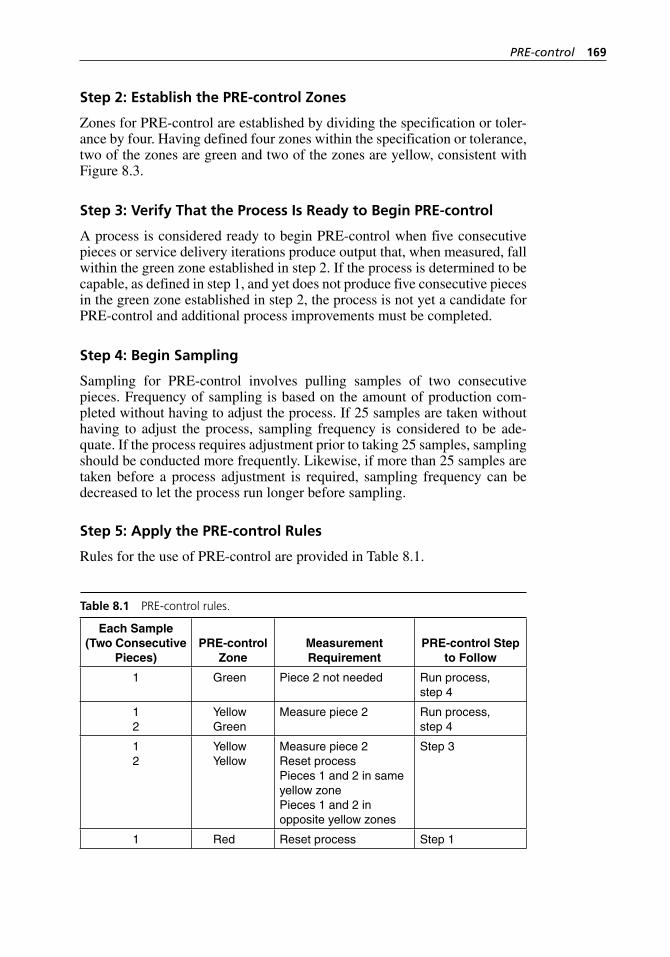
PRE-control 169
Step 2: Establish the PRE- control Zones
Zones for PRE- control are established by dividing the specification or toler-ance by four. Having defined four zones within the specification or tolerance, two of the zones are green and two of the zones are yellow, consistent with Figure 8.3.
Step 3: Verify That the Process Is Ready to Begin PRE- control
A process is considered ready to begin PRE- control when five consecutive pieces or service delivery iterations produce output that, when measured, fall within the green zone established in step 2. If the process is determined to be capable, as defined in step 1, and yet does not produce five consecutive pieces in the green zone established in step 2, the process is not yet a candidate for PRE- control and additional process improvements must be completed.
Step 4: Begin Sampling
Sampling for PRE- control involves pulling samples of two consecutive pieces. Frequency of sampling is based on the amount of production com-pleted without having to adjust the process. If 25 samples are taken without having to adjust the process, sampling frequency is considered to be ade-quate. If the process requires adjustment prior to taking 25 samples, sampling should be conducted more frequently. Likewise, if more than 25 samples are taken before a process adjustment is required, sampling frequency can be decreased to let the process run longer before sampling.
Step 5: Apply the PRE- control Rules
Rules for the use of PRE- control are provided in Table 8.1.
Table 8.1 PRE- control rules.
Each Sample (Two Consecutive
Pieces)PRE-control
ZoneMeasurement Requirement
PRE-control Step to Follow
1 Green Piece 2 not needed Run process, step 4
12
YellowGreen
Measure piece 2 Run process, step 4
12
YellowYellow
Measure piece 2Reset processPieces 1 and 2 in same yellow zonePieces 1 and 2 in opposite yellow zones
Step 3
1 Red Reset process Step 1
H1277 ch08.indd 169H1277 ch08.indd 169 3/8/07 12:37:40 PM3/8/07 12:37:40 PM
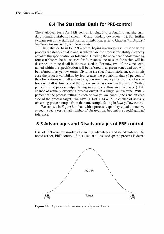
170 Chapter Eight
8.4 The Statistical Basis for PRE- control
The statistical basis for PRE- control is related to probability and the stan-dard normal distribution (mean = 0 and standard deviation = 1). For further explanation of the standard normal distribution, refer to Chapter 7 in Applied Statistics for the Six Sigma Green Belt.
The statistical basis for PRE- control begins in a worst- case situation with a process capability equal to one, in which case the process variability is exactly equal to the specification or tolerance. Dividing the specification/tolerance by four establishes the boundaries for four zones, the reasons for which will be described in more detail in the next section. For now, two of the zones con-tained within the specification will be referred to as green zones and two will be referred to as yellow zones. Dividing the specification/tolerance, or in this case the process variability, by four creates the probability that 86 percent of the observations will fall within the green zones and 7 percent of the observa-tions will fall within each of the yellow zones, as shown in Figure 8.3. With 7 percent of the process output falling in a single yellow zone, we have (1/14) chance of actually observing process output in a single yellow zone. With 7 percent of the process falling in each of two yellow zones (one zone on each side of the process target), we have (1/14)(1/14) = 1/196 chance of actually observing process output from the same sample falling in both yellow zones.
We can see in Figure 8.4 that, with a process capability equal to one, we expect to see a very small number of observations beyond the specifications/tolerance.
8.5 Advantages and Disadvantages of PRE- control
Use of PRE- control involves balancing advantages and disadvantages. As noted earlier, PRE- control, if it is used at all, is used after a process is deter-
LNTLLSL USL
UNTLTarget
99.74%
Figure 8.4 A process with process capability equal to one.
H1277 ch08.indd 170H1277 ch08.indd 170 3/8/07 12:37:40 PM3/8/07 12:37:40 PM
PRE-control 171
mined to be capable and operating in a state of statistical control. Addition-ally, PRE- control has its supporters and critics. Therefore, one must consider and balance these advantages and disadvantages prior to using PRE- control.
8.5.1 Advantages of PRE- control
Conditions may warrant the use of PRE- control, as has been discussed throughout this chapter. The following list provides the advantages of using this SQC tool:
It is much easier for shop- floor operators to use than SPC
There is a cost savings from reduced measurement, as compared with SPC
The measurement devices needed to support PRE- control (go/no-go gages) are less expensive than measurement devices for continuous variables
PRE-control does not require computation and charting, as does SPC
PRE-control provides process performance data faster than SPC does (remember that SPC requires 25 subgroups/samples to be drawn, control limits to be calculated, and charting to be completed before any conclusions can be made about process performance)
PRE-control is designed to ensure that defective products and ser-vices do not reach the customer (as compared with SPC, which is designed to detect assignable cause variation)
8.5.2 Disadvantages of PRE- control
PRE- control also presents certain disadvantages when compared with other SQC tools such as SPC. Montgomery (2005a, 475) summarizes these disadvantages:
Because SPC is commonly discontinued when PRE- control begins, diagnostic information contained as patterns of assignable cause variation in control charts is lost
Historical records of process performance (that is, records of why assignable cause variation occurred) over time are lost
Small sample sizes with PRE- control reduce the ability to detect “even moderate- to-large shifts”
PRE-control provides no information helpful in establishing statisti-cal control or in reducing variability
PRE-control is extremely sensitive to deviations from being in statis-tical control and being capable
•
•
•
•
•
•
•
•
•
•
•
H1277 ch08.indd 171H1277 ch08.indd 171 3/8/07 12:37:40 PM3/8/07 12:37:40 PM
172 Chapter Eight
PRE-control “will likely lead to unnecessary tampering with the process”
PRE-control will have “more false alarms or more missed signals than the control chart” (Wheeler and Chambers 1992, 82)
8.6 What Comes After PRE- control?
In Chapter 1 a point was made that the use of SQC tools should be tailored to the specific needs of a situation. This tailoring referred to how the various SQC tools are designed, implemented, and interpreted. This tailoring also referred to the use of the SQC tools relative to each other. Figure 1.1, and later Figure 8.1, was provided to help show the relationship among the SQC tools.
A quick review of Figure 8.1 reveals that use of acceptance sampling follows use of either (1) capability analysis and SPC, or (2) PRE- control. Acceptance sampling for variables and attributes is the subject of Chapter 9.
It should be noted that in order for acceptance sampling to be a valid SQC tool, there must be some objective evidence that a process is operat-ing in a state of statistical control, is determined to be capable, and exhibits an acceptably low defect rate. It should also be noted that use of acceptance sampling may not be required to support production operations, because the consumer may elect not to use this SQC tool, perhaps in favor of mutually supportive, long- term supplier relationships based on the use of other tools, techniques, or methods.
•
•
H1277 ch08.indd 172H1277 ch08.indd 172 3/8/07 12:37:40 PM3/8/07 12:37:40 PM
173
9.1 The Intent of Acceptance Sampling1
Acceptance sampling is a method for inspecting a product. Inspection can be done with screening (also called sorting, or 100 percent inspection), in which all units are inspected, or with sampling. Acceptance sampling is the process of inspecting a portion of the product in a lot for the purpose of mak-ing a decision regarding classification of the entire lot as either conforming or nonconforming to quality specifications.
Whether inspection is done with screening or with sampling, the results can be used for different purposes, as follows:
1. To distinguish between good lots and bad lots using acceptance sampling plans (as in incoming material inspection and final product inspection).
2. To distinguish between good products and bad products.
3. To determine the status of process control and whether the process is changing. This is usually done in conjunction with control charts.
4. To evaluate process capability. In this case, inspection is used to determine whether the process exhibits excessive variation and whether it is approaching or exceeding the specification limits.
5. To determine process adjustment. Based on inspection results of process output, as depicted by a histogram, for example, the process mean may require adjustment and/or process variation may need to be reduced. A process might require adjustment even though all the units produced to date conform to the quality standards agreed upon with the customer.
Originally published in a slightly different form in R. W. Berger, D. W. Benbow, A. K. Elshen-nawy, and H. F. Walker, eds., The Certified Quality Engineer Handbook, 2nd ed. (Milwaukee, WI: ASQ Quality Press, 2007), 190–242. Reprinted with permission.
9
Acceptance Sampling
H1277 ch09.indd 173H1277 ch09.indd 173 3/8/07 12:38:07 PM3/8/07 12:38:07 PM
174 Chapter Nine
6. To rate the accuracy of inspectors or inspection equipment by comparing the inspection results with the corresponding standards. An inspection operation can result in two types of error: classification of a conforming unit as nonconforming and classification of a nonconforming unit as conforming. The probabilities of both types of errors can be easily estimated using probability theory and other statistical methods.
7. To serve as a mechanism for evaluating vendors in terms of their products’ quality. Vendors that consistently deliver high- quality products can receive preferred status involving reduced inspection and priority in bidding for new contracts, while vendors that do not stand up to quality requirements could be warned or discontinued altogether. This type of procedure is known as vendor qualification or vendor certification.
The last three uses of inspection might be seen as feedback about the produc-tion processes, the measurement processes, and the supplier.
9.2 Sampling Inspection versus 100 Percent Inspection
Sampling provides the economic advantage of lower inspection costs due to fewer units being inspected. In addition, the time required to inspect a sample is substantially less than that required for the entire lot, and there is less damage to the product due to reduced handling. Most inspectors find that selection and inspection of a random sample is less tedious and monotonous than inspection of the complete lot. Another advantage of sampling inspec-tion is related to the supplier/customer relationship. By inspecting a small fraction of the lot and forcing the supplier to screen 100 percent in case of lot rejection (which is the case for rectifying inspection), the customer empha-sizes that the supplier must be concerned with quality. On the other hand, the variability inherent in sampling results in sampling errors: rejection of lots of conforming quality and acceptance of lots of nonconforming quality.
Acceptance sampling is most appropriate when inspection costs are high and when 100 percent inspection is monotonous and can cause inspec-tor fatigue and boredom, resulting in degraded performance and increased error rates. Obviously, sampling is the only choice available for destructive inspection. Rectifying sampling is a form of acceptance sampling. Sample units detected as nonconforming are discarded from the lot, replaced with conforming units, or repaired. Rejected lots are subject to 100 percent screen-ing, which can involve discarding, replacing, or repairing units detected as nonconforming.
In certain situations, it is preferable to inspect 100 percent of the prod-uct. This would be the case for critical or complex products, where the cost of making the wrong decision would be too high. Screening is appropriate when the fraction nonconforming is extremely high. In this case, most of the
H1277 ch09.indd 174H1277 ch09.indd 174 3/8/07 12:38:07 PM3/8/07 12:38:07 PM
Acceptance Sampling 175
lots would be rejected under acceptance sampling, and those accepted would be so as a result of statistical variations rather than better quality. Screening is also appropriate when the fraction nonconforming is not known and an estimate based on a large sample is needed.
9.3 Sampling Concepts
Sampling may be performed according to the type of quality characteristics to be inspected. There are three major categories of sampling plans: sampling plans for attributes, sampling plans for variables, and special sampling plans. It should be noted that acceptance sampling is not advised for processes in continuous production and in a state of statistical control. For these processes, Deming provides decision rules for selecting either 100 percent inspection or no inspection.1
9.3.1 Lot- by-Lot versus Average Quality Protection
For continuing processes, sampling plans based on average quality protection have characteristics calculated from the binomial and/or Poisson distribu-tions. For processes not considered to be continuing, sampling plans based on lot- by-lot protection have characteristics calculated from the hypergeometric distribution, which takes the lot size into consideration.
Sampling plans based on the Poisson and binomial distributions are more common than those based on the hypergeometric distribution. This is due to the complexity of calculating plans based on the hypergeometric distri-bution. New software on personal computers, however, may eliminate this drawback.
9.3.2 The OC Curve
No matter which type of attribute sampling plan is considered, the most important evaluation tool is the OC curve.
The OC curve allows a sampling plan to be almost completely evalu-ated at a glance, giving a pictorial view of the probabilities of accepting lots submitted at varying levels of percent defective. The OC curve illustrates the risks involved in acceptance sampling. Figure 9.1 shows an OC curve for a sample size n of 50 drawn from an infinite lot size, with an acceptance number c of 3.
As can be seen by the OC curve, if the lot were 100 percent to specifica-tions, the probability of acceptance Pa would also be 100 percent. But if the lot were 13.4 percent defective, there would be a 10 percent probability of acceptance. There are two types of OC curves to consider: (1) type A OC curves and (2) type B OC curves. Type A OC curves are used to calculate the probability of acceptance on a lot- by-lot basis when the lot is not a product of a continuous process. These OC curves are calculated using the hypergeo-metric distribution.
H1277 ch09.indd 175H1277 ch09.indd 175 3/8/07 12:38:07 PM3/8/07 12:38:07 PM
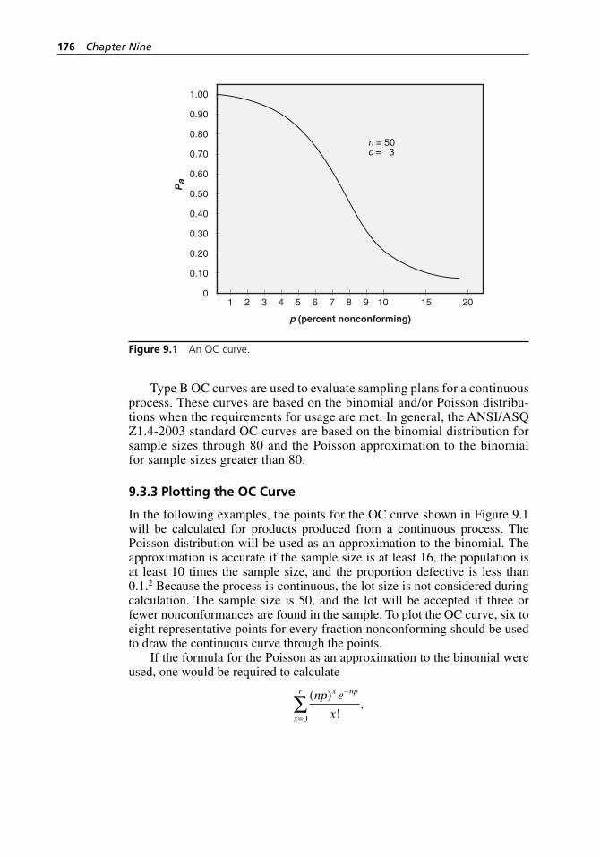
176 Chapter Nine
Type B OC curves are used to evaluate sampling plans for a continuous process. These curves are based on the binomial and/or Poisson distribu-tions when the requirements for usage are met. In general, the ANSI/ASQ Z1.4-2003 standard OC curves are based on the binomial distribution for sample sizes through 80 and the Poisson approximation to the binomial for sample sizes greater than 80.
9.3.3 Plotting the OC Curve
In the following examples, the points for the OC curve shown in Figure 9.1 will be calculated for products produced from a continuous process. The Poisson distribution will be used as an approximation to the binomial. The approximation is accurate if the sample size is at least 16, the population is at least 10 times the sample size, and the proportion defective is less than 0.1.2 Because the process is continuous, the lot size is not considered during calculation. The sample size is 50, and the lot will be accepted if three or fewer nonconformances are found in the sample. To plot the OC curve, six to eight representative points for every fraction nonconforming should be used to draw the continuous curve through the points.
If the formula for the Poisson as an approximation to the binomial were used, one would be required to calculate
( )
!,
–np e
x
x np
x
r
=∑
0
0
0.10
1 2 3 4 5 6 7 8 9 10 15
n = 50c = 3
20
0.20
0.30
0.40
0.50
0.60
0.70
Pa
p (percent nonconforming)
0.80
0.90
1.00
Figure 9.1 An OC curve.
H1277 ch09.indd 176H1277 ch09.indd 176 3/8/07 12:38:08 PM3/8/07 12:38:08 PM
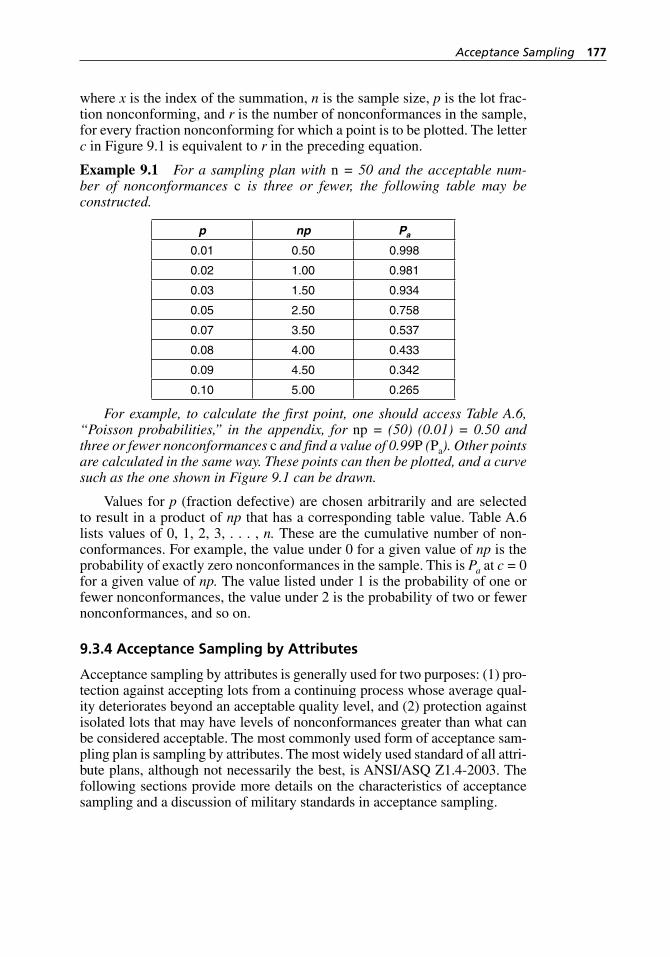
Acceptance Sampling 177
where x is the index of the summation, n is the sample size, p is the lot frac-tion nonconforming, and r is the number of nonconformances in the sample, for every fraction nonconforming for which a point is to be plotted. The letter c in Figure 9.1 is equivalent to r in the preceding equation.
Example 9.1 For a sampling plan with n = 50 and the acceptable num-ber of nonconformances c is three or fewer, the following table may be constructed.
p np Pa
0.01 0.50 0.998
0.02 1.00 0.981
0.03 1.50 0.934
0.05 2.50 0.758
0.07 3.50 0.537
0.08 4.00 0.433
0.09 4.50 0.342
0.10 5.00 0.265
For example, to calculate the first point, one should access Table A.6, “Poisson probabilities,” in the appendix, for np = (50) (0.01) = 0.50 and three or fewer nonconformances c and find a value of 0.99P (Pa). Other points are calculated in the same way. These points can then be plotted, and a curve such as the one shown in Figure 9.1 can be drawn.
Values for p (fraction defective) are chosen arbitrarily and are selected to result in a product of np that has a corresponding table value. Table A.6 lists values of 0, 1, 2, 3, . . . , n. These are the cumulative number of non-conformances. For example, the value under 0 for a given value of np is the probability of exactly zero nonconformances in the sample. This is Pa at c = 0 for a given value of np. The value listed under 1 is the probability of one or fewer nonconformances, the value under 2 is the probability of two or fewer nonconformances, and so on.
9.3.4 Acceptance Sampling by Attributes
Acceptance sampling by attributes is generally used for two purposes: (1) pro-tection against accepting lots from a continuing process whose average qual-ity deteriorates beyond an acceptable quality level, and (2) protection against isolated lots that may have levels of nonconformances greater than what can be considered acceptable. The most commonly used form of acceptance sam-pling plan is sampling by attributes. The most widely used standard of all attri-bute plans, although not necessarily the best, is ANSI/ASQ Z1.4-2003. The following sections provide more details on the characteristics of acceptance sampling and a discussion of military standards in acceptance sampling.
H1277 ch09.indd 177H1277 ch09.indd 177 3/8/07 12:38:08 PM3/8/07 12:38:08 PM
178 Chapter Nine
9.3.5 Acceptable Quality Limit
As part of the revision of ANSI/ASQC Z1.4-1993, acceptable quality level (AQL) has been changed to acceptable quality limit (AQL) in ANSI/ASQ Z1.4-2003 and is defined as the quality level that is the worst tolerable process average when a continuing series of lots is submitted for acceptance sam-pling. This means that a lot that has a fraction defective equal to the AQL has a high probability (generally in the area of 0.95, although it may vary) of being accepted. As a result, plans that are based on AQL, such as ANSI/ASQ Z1.4-2003, favor the producer in getting lots accepted that are in the general neighborhood of the AQL for fraction defective in a lot.
9.3.6 Lot Tolerance Percent Defective
The lot tolerance percent defective (LTPD), expressed in percent defective, is the poorest quality in an individual lot that should be accepted. The LTPD has a low probability of acceptance. In many sampling plans, the LTPD is the percent defective having a 10 percent probability of acceptance.
9.3.7 Producer’s and Consumer’s Risks
There are risks involved in using acceptance sampling plans. These risks are (1) producer’s risk and (2) consumer’s risk. These risks correspond with Type I and Type II errors in hypothesis testing. The definitions of producer’s and consumer’s risks are:
Producer’s risk (α). The producer’s risk for any given sampling plan is the probability of rejecting a lot that is within the acceptable qual-ity level.3 This means that the producer faces the possibility (at level of significance α) of having a lot rejected even though the lot has met the requirements stipulated by the AQL level.
Consumer’s risk (β). The consumer’s risk for any given sampling plan is the probability of acceptance (usually 10 percent) for a designated numerical value of relatively poor submitted quality.4 The consumer’s risk, therefore, is the probability of accepting a lot that has a quality level equal to the LTPD.
9.3.8 Average Outgoing Quality
The average outgoing quality (AOQ) is the expected average quality of out-going products, including all accepted lots, plus all rejected lots that have been sorted 100 percent and have had all the nonconforming units replaced by conforming units.
There is a given AOQ for specific fractions nonconforming of submitted lots sampled under a given sampling plan. When the fraction nonconforming is very low, a large majority of the lots will be accepted as submitted. The few lots that are rejected will be sorted 100 percent and have all nonconforming units replaced with conforming units. Thus, the AOQ will always be less than
H1277 ch09.indd 178H1277 ch09.indd 178 3/8/07 12:38:08 PM3/8/07 12:38:08 PM
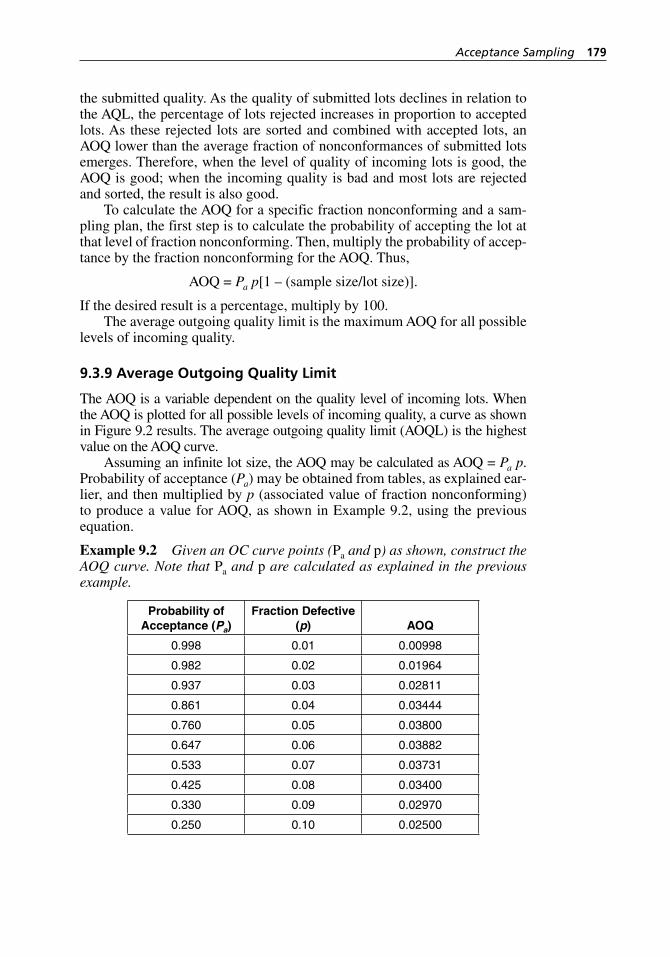
Acceptance Sampling 179
the submitted quality. As the quality of submitted lots declines in relation to the AQL, the percentage of lots rejected increases in proportion to accepted lots. As these rejected lots are sorted and combined with accepted lots, an AOQ lower than the average fraction of nonconformances of submitted lots emerges. Therefore, when the level of quality of incoming lots is good, the AOQ is good; when the incoming quality is bad and most lots are rejected and sorted, the result is also good.
To calculate the AOQ for a specific fraction nonconforming and a sam-pling plan, the first step is to calculate the probability of accepting the lot at that level of fraction nonconforming. Then, multiply the probability of accep-tance by the fraction nonconforming for the AOQ. Thus,
AOQ = Pa p[1 – (sample size/lot size)].
If the desired result is a percentage, multiply by 100.The average outgoing quality limit is the maximum AOQ for all possible
levels of incoming quality.
9.3.9 Average Outgoing Quality Limit
The AOQ is a variable dependent on the quality level of incoming lots. When the AOQ is plotted for all possible levels of incoming quality, a curve as shown in Figure 9.2 results. The average outgoing quality limit (AOQL) is the highest value on the AOQ curve.
Assuming an infinite lot size, the AOQ may be calculated as AOQ = Pa p. Probability of acceptance (Pa) may be obtained from tables, as explained ear-lier, and then multiplied by p (associated value of fraction nonconforming) to produce a value for AOQ, as shown in Example 9.2, using the previous equation.
Example 9.2 Given an OC curve points (Pa and p) as shown, construct the AOQ curve. Note that Pa and p are calculated as explained in the previous example.
Probability of Acceptance (Pa)
Fraction Defective (p) AOQ
0.998 0.01 0.00998
0.982 0.02 0.01964
0.937 0.03 0.02811
0.861 0.04 0.03444
0.760 0.05 0.03800
0.647 0.06 0.03882
0.533 0.07 0.03731
0.425 0.08 0.03400
0.330 0.09 0.02970
0.250 0.10 0.02500
H1277 ch09.indd 179H1277 ch09.indd 179 3/8/07 12:38:08 PM3/8/07 12:38:08 PM
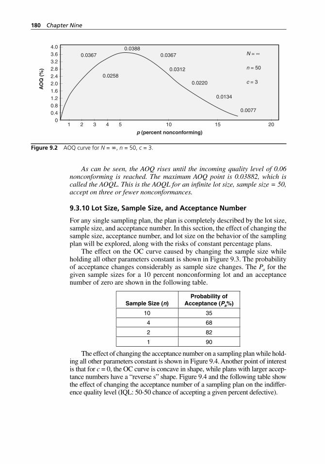
180 Chapter Nine
As can be seen, the AOQ rises until the incoming quality level of 0.06 nonconforming is reached. The maximum AOQ point is 0.03882, which is called the AOQL. This is the AOQL for an infinite lot size, sample size = 50, accept on three or fewer nonconformances.
9.3.10 Lot Size, Sample Size, and Acceptance Number
For any single sampling plan, the plan is completely described by the lot size, sample size, and acceptance number. In this section, the effect of changing the sample size, acceptance number, and lot size on the behavior of the sampling plan will be explored, along with the risks of constant percentage plans.
The effect on the OC curve caused by changing the sample size while holding all other parameters constant is shown in Figure 9.3. The probability of acceptance changes considerably as sample size changes. The Pa for the given sample sizes for a 10 percent nonconforming lot and an acceptance number of zero are shown in the following table.
Sample Size (n)Probability of
Acceptance (Pa%)
10 35
4 68
2 82
1 90
The effect of changing the acceptance number on a sampling plan while hold-ing all other parameters constant is shown in Figure 9.4. Another point of interest is that for c = 0, the OC curve is concave in shape, while plans with larger accep-tance numbers have a “reverse s” shape. Figure 9.4 and the following table show the effect of changing the acceptance number of a sampling plan on the indiffer-ence quality level (IQL: 50-50 chance of accepting a given percent defective).
1 2 3 4 5
0.0367
0.0258
0.03880.0367
0.0312
0.0220
0.0134
0.0077
10 15 20
N = ∞
n = 50
c = 3
4.03.63.22.82.42.01.61.20.80.4
0
p (percent nonconforming)
AO
Q (
%)
Figure 9.2 AOQ curve for N = ∞, n = 50, c = 3.
H1277 ch09.indd 180H1277 ch09.indd 180 3/8/07 12:38:08 PM3/8/07 12:38:08 PM
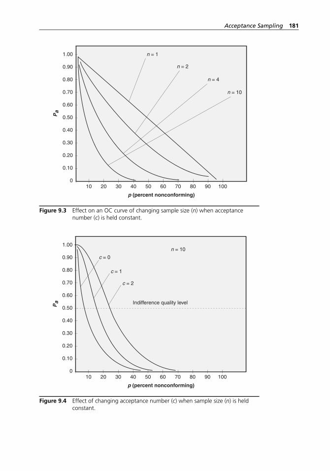
Acceptance Sampling 181
0
0.10
10 20 30 40 50 60 70 80 90 100
n = 1
n = 2
n = 4
n = 10
0.20
0.30
0.40
0.50
0.60
0.70
Pa
p (percent nonconforming)
0.80
0.90
1.00
Figure 9.3 Effect on an OC curve of changing sample size (n) when acceptance number (c) is held constant.
0
0.10
10 20 30 40 50 60 70 80 90 100
c = 0
c = 1
c = 2
n = 10
Indifference quality level
0.20
0.30
0.40
0.50
0.60
0.70
Pa
p (percent nonconforming)
0.80
0.90
1.00
Figure 9.4 Effect of changing acceptance number (c) when sample size (n) is held constant.
H1277 ch09.indd 181H1277 ch09.indd 181 3/8/07 12:38:08 PM3/8/07 12:38:08 PM
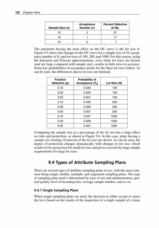
182 Chapter Nine
Sample Size (n)Acceptance Number (c)
Percent Defective at IQL
10 2 27
10 1 17
10 0 7
The parameter having the least effect on the OC curve is the lot size N. Figure 9.5 shows the changes in the OC curve for a sample size of 10, accep-tance number of 0, and lot sizes of 100, 200, and 1000. For this reason, using the binomial and Poisson approximations, even when lot sizes are known (and are large compared with sample size), results in little error in accuracy. Some key probabilities of acceptance points for the three lot sizes follow. As can be seen, the differences due to lot size are minimal.
Fraction Defective (p)
Probability of Acceptance (Pa) Lot Size (N)
0.10 0.330 100
0.30 0.023 100
0.50 0.001 100
0.10 0.340 200
0.30 0.026 200
0.50 0.001 200
0.10 0.347 1000
0.30 0.028 1000
0.50 0.001 1000
Computing the sample size as a percentage of the lot size has a large effect on risks and protection, as shown in Figure 9.6. In this case, plans having a sample size totaling 10 percent of the lot size are shown. As can be seen, the degree of protection changes dramatically with changes in lot size, which results in low protection for small lot sizes and gives excessively large sample requirements for large lot sizes.
9.4 Types of Attribute Sampling Plans
There are several types of attribute sampling plans in use, with the most com-mon being single, double, multiple, and sequential sampling plans. The type of sampling plan used is determined by ease of use and administration, gen-eral quality level of incoming lots, average sample number, and so on.
9.4.1 Single Sampling Plans
When single sampling plans are used, the decision to either accept or reject the lot is based on the results of the inspection of a single sample of n items
H1277 ch09.indd 182H1277 ch09.indd 182 3/8/07 12:38:09 PM3/8/07 12:38:09 PM
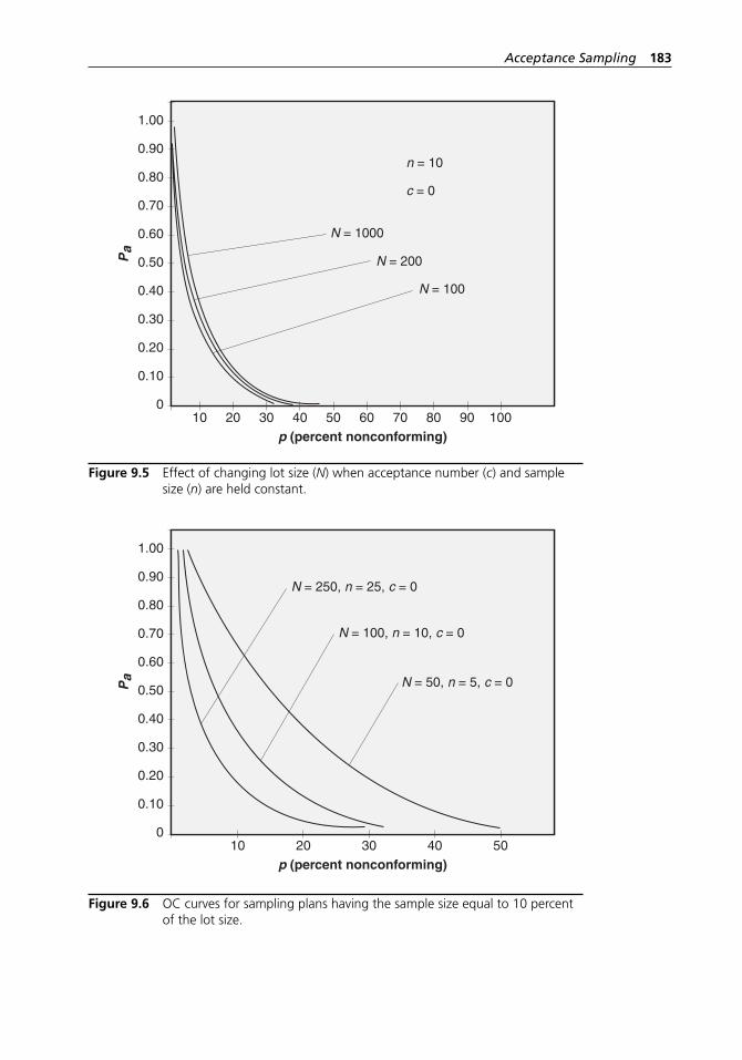
Acceptance Sampling 183
0
0.10
10 20 30 40 50 60 70 80 90 100
N = 1000
N = 200
N = 100
n = 10
c = 0
0.20
0.30
0.40
0.50
0.60
0.70
Pa
p (percent nonconforming)
0.80
0.90
1.00
Figure 9.5 Effect of changing lot size (N) when acceptance number (c) and sample size (n) are held constant.
0
0.10
10 20 30 40 50
N = 250, n = 25, c = 0
N = 100, n = 10, c = 0
N = 50, n = 5, c = 0
0.20
0.30
0.40
0.50
0.60
0.70
Pa
p (percent nonconforming)
0.80
0.90
1.00
Figure 9.6 OC curves for sampling plans having the sample size equal to 10 percent of the lot size.
H1277 ch09.indd 183H1277 ch09.indd 183 3/8/07 12:38:09 PM3/8/07 12:38:09 PM
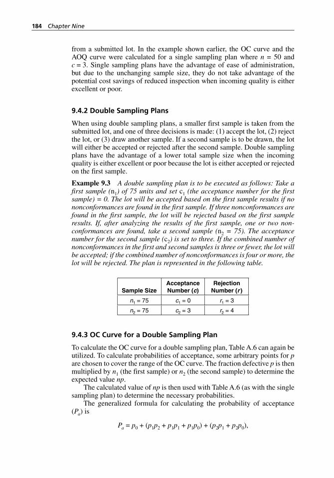
184 Chapter Nine
from a submitted lot. In the example shown earlier, the OC curve and the AOQ curve were calculated for a single sampling plan where n = 50 and c = 3. Single sampling plans have the advantage of ease of administration, but due to the unchanging sample size, they do not take advantage of the potential cost savings of reduced inspection when incoming quality is either excellent or poor.
9.4.2 Double Sampling Plans
When using double sampling plans, a smaller first sample is taken from the submitted lot, and one of three decisions is made: (1) accept the lot, (2) reject the lot, or (3) draw another sample. If a second sample is to be drawn, the lot will either be accepted or rejected after the second sample. Double sampling plans have the advantage of a lower total sample size when the incoming quality is either excellent or poor because the lot is either accepted or rejected on the first sample.
Example 9.3 A double sampling plan is to be executed as follows: Take a first sample (n1) of 75 units and set c1 (the acceptance number for the first sample) = 0. The lot will be accepted based on the first sample results if no nonconformances are found in the first sample. If three nonconformances are found in the first sample, the lot will be rejected based on the first sample results. If, after analyzing the results of the first sample, one or two non-conformances are found, take a second sample (n2 = 75). The acceptance number for the second sample (c2) is set to three. If the combined number of nonconformances in the first and second samples is three or fewer, the lot will be accepted; if the combined number of nonconformances is four or more, the lot will be rejected. The plan is represented in the following table.
Sample SizeAcceptance Number (c)
Rejection Number (r )
n1 = 75 c1 = 0 r1 = 3
n2 = 75 c2 = 3 r2 = 4
9.4.3 OC Curve for a Double Sampling Plan
To calculate the OC curve for a double sampling plan, Table A.6 can again be utilized. To calculate probabilities of acceptance, some arbitrary points for p are chosen to cover the range of the OC curve. The fraction defective p is then multiplied by n1 (the first sample) or n2 (the second sample) to determine the expected value np.
The calculated value of np is then used with Table A.6 (as with the single sampling plan) to determine the necessary probabilities.
The generalized formula for calculating the probability of acceptance (Pa) is
Pa = p0 + (p1p2 + p1p1 + p1p0) + (p2p1 + p2p0),
H1277 ch09.indd 184H1277 ch09.indd 184 3/8/07 12:38:09 PM3/8/07 12:38:09 PM
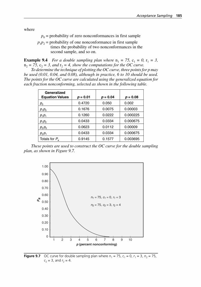
Acceptance Sampling 185
where
p0 = probability of zero nonconformances in first sample
p1p2 = probability of one nonconformance in first sample times the probability of two nonconformances in the second sample, and so on.
Example 9.4 For a double sampling plan where n1 = 75, c1 = 0, r1 = 3, n2 = 75, c2 = 3, and r2 = 4, show the computations for the OC curve.
To determine the technique of plotting the OC curve, three points for p may be used (0.01, 0.04, and 0.08), although in practice, 6 to 10 should be used. The points for the OC curve are calculated using the generalized equation for each fraction nonconforming, selected as shown in the following table.
Generalized Equation Values p = 0.01 p = 0.04 p = 0.08
p0 0.4720 0.050 0.002
p1p0 0.1676 0.0075 0.00003
p1p1 0.1260 0.0222 0.000225
p1p2 0.0433 0.0334 0.000675
p2p0 0.0623 0.0112 0.00009
p2p1 0.0433 0.0334 0.000675
Totals for Pa 0.9145 0.1577 0.003695
These points are used to construct the OC curve for the double sampling plan, as shown in Figure 9.7.
0
0.10
1 2 3 4 5 6 7 8 9 10
n1 = 75, c1 = 0, r1 = 3
n2 = 75, c2 = 3, r2 = 4
0.20
0.30
0.40
0.50
0.60
0.70
Pa
p (percent nonconforming)
0.80
0.90
1.00
Figure 9.7 OC curve for double sampling plan where n1 = 75, c1 = 0, r1 = 3, n2 = 75, c2 = 3, and r2 = 4.
H1277 ch09.indd 185H1277 ch09.indd 185 3/8/07 12:38:09 PM3/8/07 12:38:09 PM
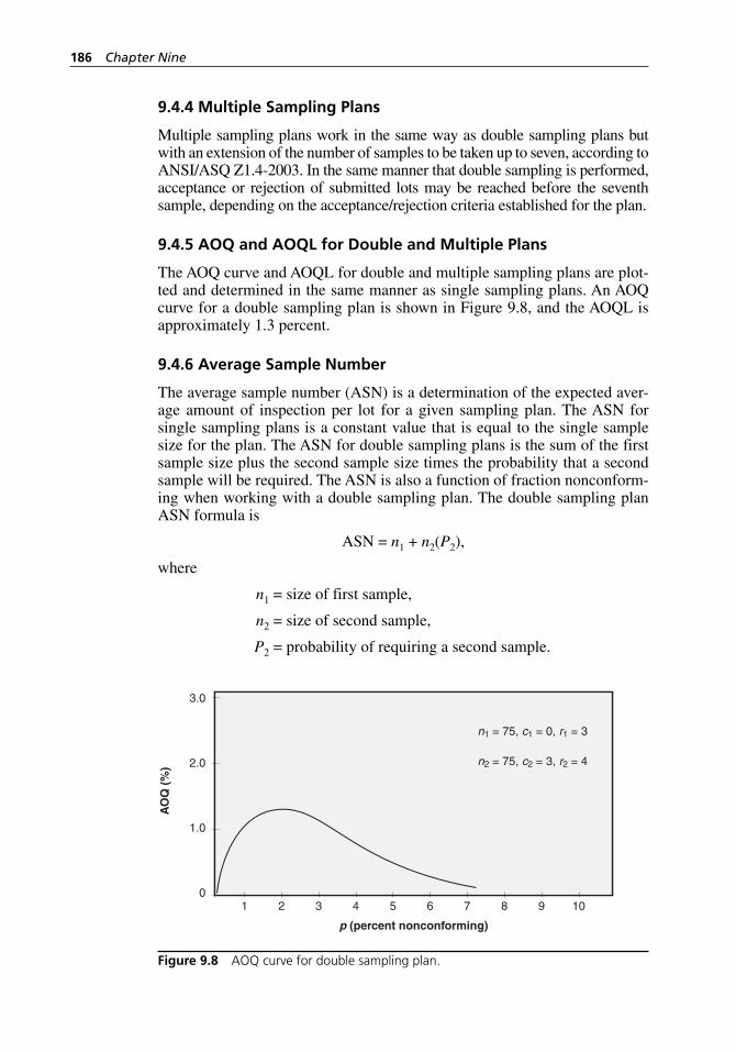
186 Chapter Nine
9.4.4 Multiple Sampling Plans
Multiple sampling plans work in the same way as double sampling plans but with an extension of the number of samples to be taken up to seven, according to ANSI/ASQ Z1.4-2003. In the same manner that double sampling is performed, acceptance or rejection of submitted lots may be reached before the seventh sample, depending on the acceptance/rejection criteria established for the plan.
9.4.5 AOQ and AOQL for Double and Multiple Plans
The AOQ curve and AOQL for double and multiple sampling plans are plot-ted and determined in the same manner as single sampling plans. An AOQ curve for a double sampling plan is shown in Figure 9.8, and the AOQL is approximately 1.3 percent.
9.4.6 Average Sample Number
The average sample number (ASN) is a determination of the expected aver-age amount of inspection per lot for a given sampling plan. The ASN for single sampling plans is a constant value that is equal to the single sample size for the plan. The ASN for double sampling plans is the sum of the first sample size plus the second sample size times the probability that a second sample will be required. The ASN is also a function of fraction nonconform-ing when working with a double sampling plan. The double sampling plan ASN formula is
ASN = n1 + n2(P2),
where
n1 = size of first sample,
n2 = size of second sample,
P2 = probability of requiring a second sample.
0
1.0
1 2 3 4 5 6 7 8 9 10
n1 = 75, c1 = 0, r1 = 3
n2 = 75, c2 = 3, r2 = 42.0
p (percent nonconforming)
3.0
AO
Q (
%)
Figure 9.8 AOQ curve for double sampling plan.
H1277 ch09.indd 186H1277 ch09.indd 186 3/8/07 12:38:09 PM3/8/07 12:38:09 PM
Acceptance Sampling 187
Example 9.5 The double sampling plan in the earlier section was
n1 = 75, c1 = 0, r1 = 3,
n2 = 75, c2 = 3, r2 = 4.
A second sample is required if, on the first sample, one or two non-conformances are noted
If zero nonconformances are found in the first sample, the lot is accepted
If three or more nonconformances are found in the first sample, the lot is rejected
Denote the probability of making a decision, accept or reject, on the first sample as P(D1). Then,
P(D1) = P(0) + P (3 or more),
P(0) = The probability of 0 nonconformances on the first sample,
P (3 or more) = The probability of 3 or more nonconformances on the first sample,
P2 = 1 – P(D1), then ASN = n1 + n2(P2).
When using Table A.6 to calculate the probability of three or more non-conformances, remember that the probability is given by
(1 – probability of 2 or fewer nonconformances) in the sample.
The ASN will be plotted for several values of fraction nonconforming p, and an ASN curve will be plotted. An example of the ASN calculation for the fraction nonconforming p = 0.01 is shown in the following equation. Several other points need to be plotted for other values of p. Figure 9.9 shows an ASN curve for the example.
When p = 0.01:
P(0) = Probability of 0 nonconformances in sample = 0.4724,
P (3 or more) = Probability of 3 or more nonconformances in sample = 0.0410,
P(D1) = Probability of a decision on the first sample (using the preceding equation) = 0.4724 + 0.0410 = 0.5134,
Then P2 = Probability of requiring a second sample = 1 – 0.5134 = 0.4866.
Thus, the ASN is:
ASN(0.01) = Average sample number for a lot quality p = 0.01
= n1 + n2 (P2)
= 75 + 75 (0.4866) = 111.50 or 112.
•
•
•
H1277 ch09.indd 187H1277 ch09.indd 187 3/8/07 12:38:09 PM3/8/07 12:38:09 PM
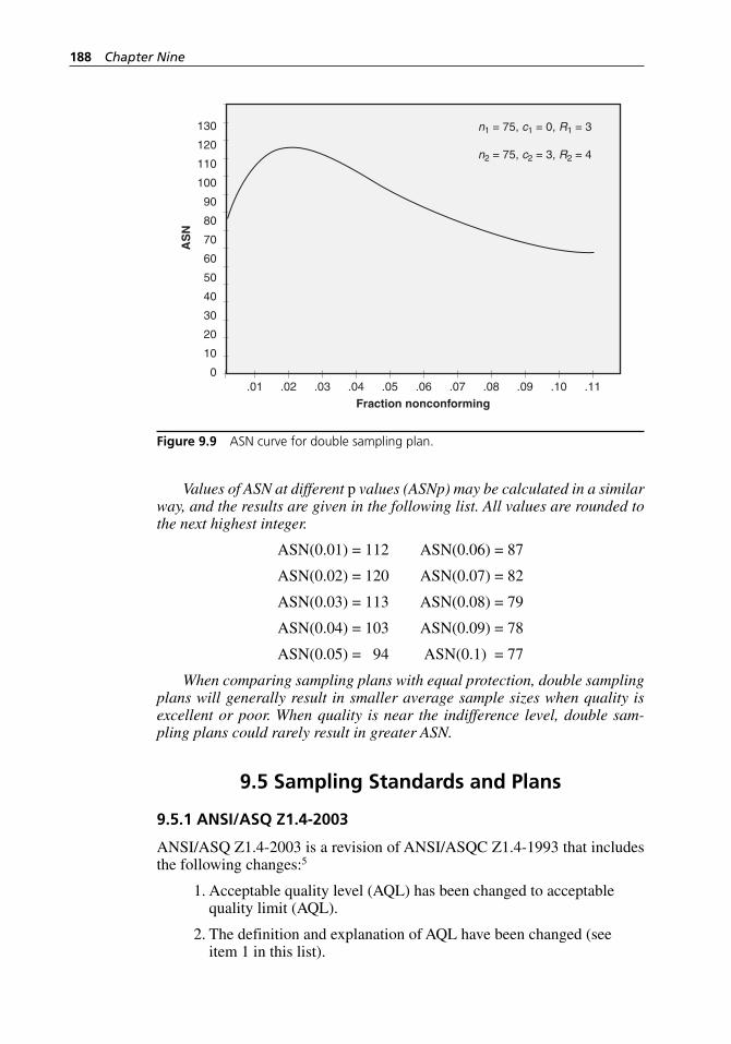
188 Chapter Nine
Values of ASN at different p values (ASNp) may be calculated in a similar way, and the results are given in the following list. All values are rounded to the next highest integer.
ASN(0.01) = 112 ASN(0.06) = 87
ASN(0.02) = 120 ASN(0.07) = 82
ASN(0.03) = 113 ASN(0.08) = 79
ASN(0.04) = 103 ASN(0.09) = 78
ASN(0.05) = 94 ASN(0.1) = 77
When comparing sampling plans with equal protection, double sampling plans will generally result in smaller average sample sizes when quality is excellent or poor. When quality is near the indifference level, double sam-pling plans could rarely result in greater ASN.
9.5 Sampling Standards and Plans
9.5.1 ANSI/ASQ Z1.4-2003
ANSI/ASQ Z1.4-2003 is a revision of ANSI/ASQC Z1.4-1993 that includes the following changes:5
1. Acceptable quality level (AQL) has been changed to acceptable quality limit (AQL).
2. The definition and explanation of AQL have been changed (see item 1 in this list).
0
10
.01 .02 .03 .04 .05 .06 .07 .08 .09 .10 .11
n1 = 75, c1 = 0, R1 = 3
n2 = 75, c2 = 3, R2 = 4
20
30
40
50
60
70
Fraction nonconforming
80
90
100
110
120
130
AS
N
Figure 9.9 ASN curve for double sampling plan.
H1277 ch09.indd 188H1277 ch09.indd 188 3/8/07 12:38:10 PM3/8/07 12:38:10 PM
Acceptance Sampling 189
3. The discontinuation of inspection rule has been changed. See later sections in this chapter.
4. ANSI/ASQC A2-1987 has been changed to ANSI/ASQ A3534-2-1993.
5. ANSI/ASQC Q3 has been changed to ASQC Q3-1988.
Other than these changes and changes to the footnotes of some tables, all tables, table numbers, and procedures used in MIL- STD-105E (which was canceled in 1995) and ANSI/ASQC Z1.4-1993 have been retained.
ANSI/ASQ Z1.4-2003 is probably the most commonly used standard for attribute sampling plans, but its wide recognition and acceptance could be due to government contracts stipulating the standard rather than its statistical importance. Producers submitting products at a nonconformance level within AQL have a high probability of having the lot accepted by the customer.
When using ANSI/ASQ Z1.4-2003, the characteristics under consider-ation should be classified. The general classifications are critical, major, and minor defects:
A critical defect is a defect that judgment and experience indicate is likely to result in hazardous or unsafe conditions for the individuals using, maintaining, or depending on the product; or it is a defect that judgment and experience indicate is likely to prevent performance of the unit. In practice, critical characteristics are commonly inspected to an AQL level of 0.40 to 0.65 percent, if not 100 percent inspected. One hundred percent inspection is recommended for critical charac-teristics if possible. Acceptance numbers are always zero for critical defects.
A major defect is a defect other than critical that is likely to result in failure or to reduce materially the usability of the unit of product for its intended purpose. In practice, AQL levels for major defects are generally about 1 percent.
A minor defect is a defect that is not likely to reduce materially the usability of the unit of product for its intended purpose. In practice, AQL levels for minor defects generally range from 1.5 percent to 2.5 percent.
9.5.2 Levels of Inspection
There are seven levels of inspection used in ANSI/ASQ Z1.4-2003: reduced inspection, normal inspection, tightened inspection, and four levels of special inspection. The special inspection levels should be used only when small sample sizes are necessary and large risks can be tolerated. When using ANSI/ASQ Z1.4-2003, a set of switching rules must be followed as to the use of reduced, normal, and tightened inspection.
The following guidelines are taken from ANSI/ASQ Z1.4-2003:
Initiation of inspection. Normal inspection Level II will be used at the start of inspection unless otherwise directed by the responsible authority.
•
•
•
H1277 ch09.indd 189H1277 ch09.indd 189 3/8/07 12:38:10 PM3/8/07 12:38:10 PM
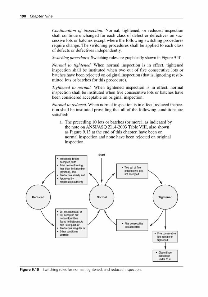
190 Chapter Nine
Continuation of inspection. Normal, tightened, or reduced inspection shall continue unchanged for each class of defect or defectives on suc-cessive lots or batches except where the following switching procedures require change. The switching procedures shall be applied to each class of defects or defectives independently.
Switching procedures. Switching rules are graphically shown in Figure 9.10.
Normal to tightened. When normal inspection is in effect, tightened inspection shall be instituted when two out of five consecutive lots or batches have been rejected on original inspection (that is, ignoring resub-mitted lots or batches for this procedure).
Tightened to normal. When tightened inspection is in effect, normal inspection shall be instituted when five consecutive lots or batches have been considered acceptable on original inspection.
Normal to reduced. When normal inspection is in effect, reduced inspec-tion shall be instituted providing that all of the following conditions are satisfied:
a. The preceding 10 lots or batches (or more), as indicated by the note on ANSI/ASQ Z1.4-2003 Table VIII, also shown as Figure 9.13 at the end of this chapter, have been on normal inspection and none have been rejected on original inspection.
• Preceding 10 lots accepted, with• Total nonconforming less than limit number (optional), and• Production steady, and• Approved by responsible authority
• Two out of five consecutive lots not accepted
• Five consecutive lots accepted
• Five consecutive lots remain on tightened
• Discontinue inspection under Z1.4
Reduced Normal
Start
Tightened
• Lot not accepted, or• Lot accepted but nonconformities found lie between Ac and Re of plan, or• Production irregular, or• Other conditions warrant
Figure 9.10 Switching rules for normal, tightened, and reduced inspection.
H1277 ch09.indd 190H1277 ch09.indd 190 3/8/07 12:38:10 PM3/8/07 12:38:10 PM
Acceptance Sampling 191
b. The total number of defectives (or defects) in the sample from the preceding 10 lots or batches (or such other number as was used for condition (a)) is equal to or less than the applicable number given in Table VIII of ANSI/ASQ Z1.4-2003 (shown as Figure 9.13 at the end of this chapter). If double or multiple sampling is in use, all samples inspected should be included, not first samples only.
c. Production is at a steady rate.
d. Reduced inspection is considered desirable by the responsible authority.
Reduced to normal. When reduced inspection is in effect, normal inspection shall be instituted if any of the following occur on original inspection:
a. A lot or batch is rejected.
b. A lot or batch is considered acceptable under reduced inspection but the sampling procedures terminated without either acceptance or rejection criteria having been met. In these circumstances, the lot or batch will be considered acceptable, but normal inspection will be reinstated starting with the new lot or batch.
c. Production becomes irregular or delayed.
d. Other conditions warrant that normal inspection shall be instituted.
Discontinuation of inspection. If the cumulative number of lots not accepted in a sequence of consecutive lots on tightened inspection reaches five, the acceptance procedures of this standard shall be discontinued. Inspection under the provisions of this standard shall not be resumed until corrective action has been taken. Tightened inspection shall then be used as “normal to tightened.”
9.5.3 Types of Sampling
ANSI/ASQ Z1.4-2003 allows for three types of sampling:
1. Single sampling
2. Double sampling
3. Multiple sampling
The choice of the type of plan depends on many variables. Single sampling is the easiest to administer and perform, but it usually results in the largest average total inspection (ATI). Double sampling results in a lower ATI than single sampling, but it requires more decisions to be made, such as:
Accept the lot after the first sample
Reject the lot after the first sample
Take a second sample
•
•
•
H1277 ch09.indd 191H1277 ch09.indd 191 3/8/07 12:38:10 PM3/8/07 12:38:10 PM
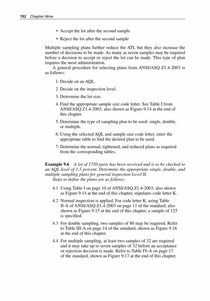
192 Chapter Nine
Accept the lot after the second sample
Reject the lot after the second sample
Multiple sampling plans further reduce the ATI, but they also increase the number of decisions to be made. As many as seven samples may be required before a decision to accept or reject the lot can be made. This type of plan requires the most administration.
A general procedure for selecting plans from ANSI/ASQ Z1.4-2003 is as follows:
1. Decide on an AQL.
2. Decide on the inspection level.
3. Determine the lot size.
4. Find the appropriate sample size code letter. See Table I from ANSI/ASQ Z1.4-2003, also shown as Figure 9.14 at the end of this chapter.
5. Determine the type of sampling plan to be used: single, double, or multiple.
6. Using the selected AQL and sample size code letter, enter the appropriate table to find the desired plan to be used.
7. Determine the normal, tightened, and reduced plans as required from the corresponding tables.
Example 9.6 A lot of 1750 parts has been received and is to be checked to an AQL level of 1.5 percent. Determine the appropriate single, double, and multiple sampling plans for general inspection Level II.
Steps to define the plans are as follows:
4.1 Using Table I on page 10 of ANSI/ASQ Z1.4-2003, also shown as Figure 9.14 at the end of this chapter, stipulates code letter K.
4.2 Normal inspection is applied. For code letter K, using Table II- A of ANSI/ASQ Z1.4-2003 on page 11 of the standard, also shown as Figure 9.15 at the end of this chapter, a sample of 125 is specified.
4.3 For double sampling, two samples of 80 may be required. Refer to Table III- A on page 14 of the standard, shown as Figure 9.16 at the end of this chapter.
4.4 For multiple sampling, at least two samples of 32 are required and it may take up to seven samples of 32 before an acceptance or rejection decision is made. Refer to Table IV- A on page 17 of the standard, shown as Figure 9.17 at the end of this chapter.
•
•
H1277 ch09.indd 192H1277 ch09.indd 192 3/8/07 12:38:10 PM3/8/07 12:38:10 PM
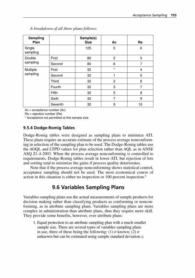
Acceptance Sampling 193
A breakdown of all three plans follows:
Sampling Plan
Sample(s) Size Ac Re
Single sampling
125 5 6
Double sampling
First 80 2 5
Second 80 6 7
Multiple sampling
First 32 * 4
Second 32 1 5
Third 32 2 6
Fourth 32 3 7
Fifth 32 5 8
Sixth 32 7 9
Seventh 32 9 10
Ac = acceptance number (Ac)Re = rejection number (Re)* Acceptance not permitted at this sample size.
9.5.4 Dodge- Romig Tables
Dodge-Romig tables were designed as sampling plans to minimize ATI. These plans require an accurate estimate of the process average nonconform-ing in selection of the sampling plan to be used. The Dodge- Romig tables use the AOQL and LTPD values for plan selection rather than AQL as in ANSI/ASQ Z1.4-2003. When the process average nonconforming is controlled to requirements, Dodge- Romig tables result in lower ATI, but rejection of lots and sorting tend to minimize the gains if process quality deteriorates.
Note that if the process average nonconforming shows statistical control, acceptance sampling should not be used. The most economical course of action in this situation is either no inspection or 100 percent inspection.6
9.6 Variables Sampling Plans
Variables sampling plans use the actual measurements of sample products for decision making rather than classifying products as conforming or noncon-forming, as in attribute sampling plans. Variables sampling plans are more complex in administration than attribute plans, thus they require more skill. They provide some benefits, however, over attribute plans:
1. Equal protection to an attribute sampling plan with a much smaller sample size. There are several types of variables sampling plans in use, three of these being the following: (1) σ known; (2) σ unknown but can be estimated using sample standard deviation s;
H1277 ch09.indd 193H1277 ch09.indd 193 3/8/07 12:38:10 PM3/8/07 12:38:10 PM
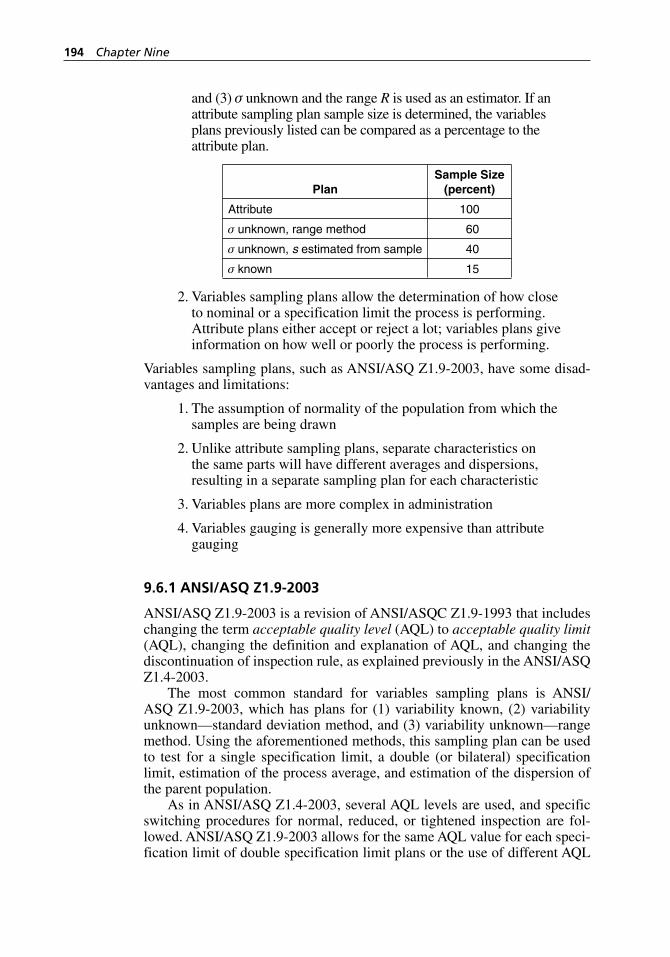
194 Chapter Nine
and (3) σ unknown and the range R is used as an estimator. If an attribute sampling plan sample size is determined, the variables plans previously listed can be compared as a percentage to the attribute plan.
PlanSample Size
(percent)
Attribute 100
σ unknown, range method 60
σ unknown, s estimated from sample 40
σ known 15
2. Variables sampling plans allow the determination of how close to nominal or a specification limit the process is performing. Attribute plans either accept or reject a lot; variables plans give information on how well or poorly the process is performing.
Variables sampling plans, such as ANSI/ASQ Z1.9-2003, have some disad-vantages and limitations:
1. The assumption of normality of the population from which the samples are being drawn
2. Unlike attribute sampling plans, separate characteristics on the same parts will have different averages and dispersions, resulting in a separate sampling plan for each characteristic
3. Variables plans are more complex in administration
4. Variables gauging is generally more expensive than attribute gauging
9.6.1 ANSI/ASQ Z1.9-2003
ANSI/ASQ Z1.9-2003 is a revision of ANSI/ASQC Z1.9-1993 that includes changing the term acceptable quality level (AQL) to acceptable quality limit (AQL), changing the definition and explanation of AQL, and changing the discontinuation of inspection rule, as explained previously in the ANSI/ASQ Z1.4-2003.
The most common standard for variables sampling plans is ANSI/ASQ Z1.9-2003, which has plans for (1) variability known, (2) variability unknown—standard deviation method, and (3) variability unknown—range method. Using the aforementioned methods, this sampling plan can be used to test for a single specification limit, a double (or bilateral) specification limit, estimation of the process average, and estimation of the dispersion of the parent population.
As in ANSI/ASQ Z1.4-2003, several AQL levels are used, and specific switching procedures for normal, reduced, or tightened inspection are fol-lowed. ANSI/ASQ Z1.9-2003 allows for the same AQL value for each speci-fication limit of double specification limit plans or the use of different AQL
H1277 ch09.indd 194H1277 ch09.indd 194 3/8/07 12:38:10 PM3/8/07 12:38:10 PM
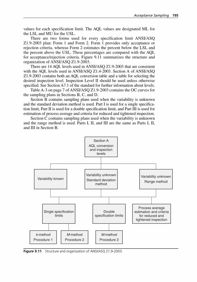
Acceptance Sampling 195
values for each specification limit. The AQL values are designated ML for the LSL and MU for the USL.
There are two forms used for every specification limit ANSI/ASQ Z1.9-2003 plan: Form 1 and Form 2. Form 1 provides only acceptance or rejection criteria, whereas Form 2 estimates the percent below the LSL and the percent above the USL. These percentages are compared with the AQL for acceptance/rejection criteria. Figure 9.11 summarizes the structure and organization of ANSI/ASQ Z1.9-2003.
There are 14 AQL levels used in ANSI/ASQ Z1.9-2003 that are consistent with the AQL levels used in ANSI/ASQ Z1.4-2003. Section A of ANSI/ASQ Z1.9-2003 contains both an AQL conversion table and a table for selecting the desired inspection level. Inspection Level II should be used unless otherwise specified. See Section A7.1 of the standard for further information about levels.
Table A-3 on page 7 of ANSI/ASQ Z1.9-2003 contains the OC curves for the sampling plans in Sections B, C, and D.
Section B contains sampling plans used when the variability is unknown and the standard deviation method is used. Part I is used for a single specifica-tion limit, Part II is used for a double specification limit, and Part III is used for estimation of process average and criteria for reduced and tightened inspection.
Section C contains sampling plans used when the variability is unknown and the range method is used. Parts I, II, and III are the same as Parts I, II, and III in Section B.
Section AAQL conversionand inspection
levels
Variability unknownStandard deviation
method
Variability known
Single specificationlimits
k-methodProcedure 1
M-methodProcedure 2
M-methodProcedure 2
Doublespecification limits
Process averageestimation and criteria
for reduced andtightened inspection
Variability unknownRange method
Figure 9.11 Structure and organization of ANSI/ASQ Z1.9-2003.
H1277 ch09.indd 195H1277 ch09.indd 195 3/8/07 12:38:11 PM3/8/07 12:38:11 PM
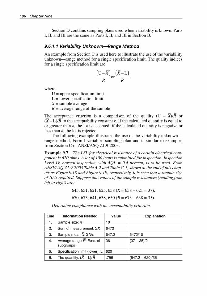
196 Chapter Nine
Section D contains sampling plans used when variability is known. Parts I, II, and III are the same as Parts I, II, and III in Section B.
9.6.1.1 Variability Unknown—Range Method
An example from Section C is used here to illustrate the use of the variability unknown—range method for a single specification limit. The quality indices for a single specification limit are
U L−( ) −( )X
R
X
Ror ,
whereU = upper specification limitL = lower specification limitX– = sample average
R– = average range of the sample
The acceptance criterion is a comparison of the quality (U – X–)/R
– or
(X– – L)/R
– to the acceptability constant k. If the calculated quantity is equal to
or greater than k, the lot is accepted; if the calculated quantity is negative or less than k, the lot is rejected.
The following example illustrates the use of the variability unknown—range method, Form I variables sampling plan and is similar to examples from Section C of ANSI/ASQ Z1.9-2003.
Example 9.7 The LSL for electrical resistance of a certain electrical com-ponent is 620 ohms. A lot of 100 items is submitted for inspection. Inspection Level IV, normal inspection, with AQL = 0.4 percent, is to be used. From ANSI/ASQ Z1.9-2003 Table A-2 and Table C-1, shown at the end of this chap-ter as Figure 9.18 and Figure 9.19, respectively, it is seen that a sample size of 10 is required. Suppose that values of the sample resistances (reading from left to right) are:
645, 651, 621, 625, 658 (R = 658 – 621 = 37),
670, 673, 641, 638, 650 (R = 673 – 638 = 35).
Determine compliance with the acceptability criterion.
Line Information Needed Value Explanation
1. Sample size: n 10
2. Sum of measurement: ΣX 6472
3. Sample mean X–: ΣX/n 647.2 6472/10
4. Average range R–: R/no. of
subgroups36 (37 + 35)/2
5. Specification limit (lower): L 620
6. The quantity: (X– – L)/R
–.756 (647.2 – 620)/36
H1277 ch09.indd 196H1277 ch09.indd 196 3/8/07 12:38:11 PM3/8/07 12:38:11 PM
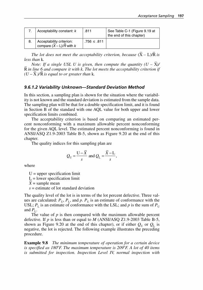
Acceptance Sampling 197
7. Acceptability constant: k .811 See Table C-1 (Figure 9.19 at the end of this chapter)
8. Acceptability criterion: compare (X
– – L)/R
– with k
.756 ≤ .811
The lot does not meet the acceptability criterion, because (X– – L)/R
– is
less than k.Note: If a single USL U is given, then compute the quantity (U – X
–)/
R– in line 6 and compare it with k. The lot meets the acceptability criterion if
(U – X– )/R
– is equal to or greater than k.
9.6.1.2 Variability Unknown—Standard Deviation Method
In this section, a sampling plan is shown for the situation where the variabil-ity is not known and the standard deviation is estimated from the sample data. The sampling plan will be that for a double specification limit, and it is found in Section B of the standard with one AQL value for both upper and lower specification limits combined.
The acceptability criterion is based on comparing an estimated per-cent nonconforming with a maximum allowable percent nonconforming for the given AQL level. The estimated percent nonconforming is found in ANSI/ASQ Z1.9-2003 Table B-5, shown as Figure 9.20 at the end of this chapter.
The quality indices for this sampling plan are
Q
X
sQ
X
sU L
U L=
−=
−and ,
where
U = upper specification limitL = lower specification limitX– = sample mean
s = estimate of lot standard deviation
The quality level of the lot is in terms of the lot percent defective. Three val-ues are calculated: PU, PL, and p. PU is an estimate of conformance with the USL; PL is an estimate of conformance with the LSL; and p is the sum of PU and PL.
The value of p is then compared with the maximum allowable percent defective. If p is less than or equal to M (ANSI/ASQ Z1.9-2003 Table B-5, shown as Figure 9.20 at the end of this chapter), or if either QU or QL is negative, the lot is rejected. The following example illustrates the preceding procedure.
Example 9.8 The minimum temperature of operation for a certain device is specified as 180°F. The maximum temperature is 209°F. A lot of 40 items is submitted for inspection. Inspection Level IV, normal inspection with
H1277 ch09.indd 197H1277 ch09.indd 197 3/8/07 12:38:11 PM3/8/07 12:38:11 PM
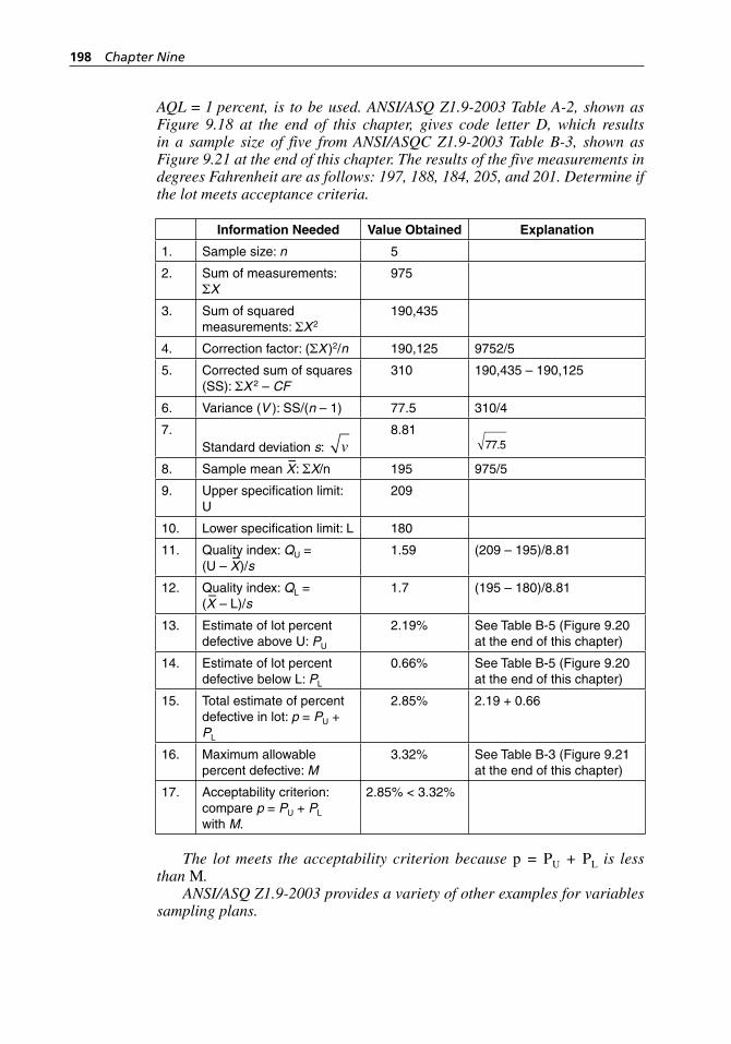
198 Chapter Nine
AQL = 1 percent, is to be used. ANSI/ASQ Z1.9-2003 Table A-2, shown as Figure 9.18 at the end of this chapter, gives code letter D, which results in a sample size of five from ANSI/ASQC Z1.9-2003 Table B-3, shown as Figure 9.21 at the end of this chapter. The results of the five measurements in degrees Fahrenheit are as follows: 197, 188, 184, 205, and 201. Determine if the lot meets acceptance criteria.
Information Needed Value Obtained Explanation
1. Sample size: n 5
2. Sum of measurements: ΣX
975
3. Sum of squared measurements: ΣX2
190,435
4. Correction factor: (ΣX )2/n 190,125 9752/5
5. Corrected sum of squares (SS): ΣX 2 – CF
310 190,435 – 190,125
6. Variance (V ): SS/(n – 1) 77.5 310/4
7.Standard deviation s: v
8.8177.5
8. Sample mean X–: ΣX/n 195 975/5
9. Upper specification limit: U
209
10. Lower specification limit: L 180
11. Quality index: QU = (U – X
–)/s
1.59 (209 – 195)/8.81
12. Quality index: QL = (X– – L)/s
1.7 (195 – 180)/8.81
13. Estimate of lot percent defective above U: PU
2.19% See Table B-5 (Figure 9.20 at the end of this chapter)
14. Estimate of lot percent defective below L: PL
0.66% See Table B-5 (Figure 9.20 at the end of this chapter)
15. Total estimate of percent defective in lot: p = PU + PL
2.85% 2.19 + 0.66
16. Maximum allowable percent defective: M
3.32% See Table B-3 (Figure 9.21 at the end of this chapter)
17. Acceptability criterion: compare p = PU + PL with M.
2.85% < 3.32%
The lot meets the acceptability criterion because p = PU + PL is less than M.
ANSI/ASQ Z1.9-2003 provides a variety of other examples for variables sampling plans.
H1277 ch09.indd 198H1277 ch09.indd 198 3/8/07 12:38:11 PM3/8/07 12:38:11 PM
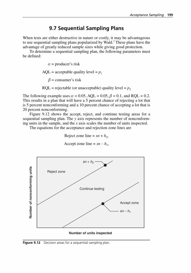
Acceptance Sampling 199
9.7 Sequential Sampling Plans
When tests are either destructive in nature or costly, it may be advantageous to use sequential sampling plans popularized by Wald.7 These plans have the advantage of greatly reduced sample sizes while giving good protection.
To determine a sequential sampling plan, the following parameters must be defined:
α = producer’s risk
AQL = acceptable quality level = p1
β = consumer’s risk
RQL = rejectable (or unacceptable) quality level = p2
The following example uses α = 0.05, AQL = 0.05, β = 0.1, and RQL = 0.2. This results in a plan that will have a 5 percent chance of rejecting a lot that is 5 percent nonconforming and a 10 percent chance of accepting a lot that is 20 percent nonconforming.
Figure 9.12 shows the accept, reject, and continue testing areas for a sequential sampling plan. The y axis represents the number of nonconform-ing units in the sample, and the x axis scales the number of units inspected.
The equations for the acceptance and rejection zone lines are
Reject zone line = sn + h2,
Accept zone line = sn – h1,
Number of units inspected
Reject zone
Continue testing
Accept zone
sn + h2
sn – h1
Nu
mb
er o
f n
on
con
form
ing
un
its
Figure 9.12 Decision areas for a sequential sampling plan.
H1277 ch09.indd 199H1277 ch09.indd 199 3/8/07 12:38:11 PM3/8/07 12:38:11 PM
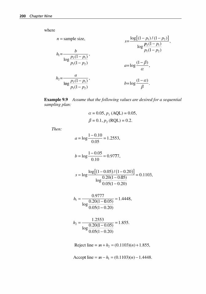
200 Chapter Nine
where
n
hb
p p
p p
ha
=
−−
sample size,
=
=
12 1
1 2
2
11
log( )( )
,
loog( )( )
,p p
p p2 1
1 2
11
−−
log ( ) / ( )
logs
p p1 21 1− −[ ]=
pp p
p p
a
b
2 1
1 2
11
1
1
( )( )
,
log( )
,
log( )
.
−−
−
−
=
=
β
α
α
β
Example 9.9 Assume that the following values are desired for a sequential sampling plan:
α = 0.05, p1 (AQL) = 0.05,
β = 0.1, p2 (RQL) = 0.2.
Then:
a
b
=−
=
=−
=
log.
.. ,
log.
..
1 0 10
0 051 2553
1 0 05
0 100 97777
1 0 05 1 0 200 20 1 0
,
loglog . / .
log. ( .
s =−( ) −( )[ ]
− 005
0 05 1 0 20
0 1103
0 97770 20 11
)
. ( . )
. ,
.
log. (
−
=
= −h00 05
0 05 1 0 20
1 4448
1 25530 202
. )
. ( . )
. ,
.
log. (
−
=
=h11 0 05
0 05 1 0 20
1 855−−
=. )
. ( . )
. .
Reject line =
Accep
sn h n+ = +2 0 1103 1 855( . )( ) . ,
tt line = − = −sn h n1 0 1103 1 4448( . )( ) . .
H1277 ch09.indd 200H1277 ch09.indd 200 3/8/07 12:38:11 PM3/8/07 12:38:11 PM
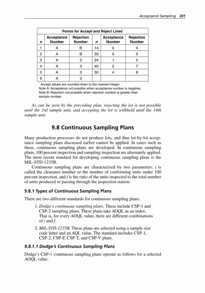
Acceptance Sampling 201
Points for Accept and Reject Lines*
nAcceptance
NumberRejection Number n
Acceptance Number
Rejection Number
1 A B 14 0 4
2 A B 20 0 5
3 A 3 24 1 5
4 A 3 40 2 7
5 A 3 50 4 8
6 A 3* Accept values are rounded down to the nearest integer.Note A: Acceptance not possible when acceptance number is negative.Note B: Rejection not possible when rejection number is greater than sample number.
As can be seen by the preceding plan, rejecting the lot is not possible until the 3rd sample unit, and accepting the lot is withheld until the 14th sample unit.
9.8 Continuous Sampling Plans
Many production processes do not produce lots, and thus lot- by-lot accep-tance sampling plans discussed earlier cannot be applied. In cases such as these, continuous sampling plans are developed. In continuous sampling plans, 100 percent inspection and sampling inspection are alternately applied. The most recent standard for developing continuous sampling plans is the MIL- STD-1235B.
Continuous sampling plans are characterized by two parameters: i is called the clearance number or the number of conforming units under 100 percent inspection, and f is the ratio of the units inspected to the total number of units produced or passing through the inspection station.
9.8.1 Types of Continuous Sampling Plans
There are two different standards for continuous sampling plans:
1. Dodge’s continuous sampling plans. These include CSP-1 and CSP-2 sampling plans. These plans take AOQL as an index. That is, for every AOQL value, there are different combinations of i and f.
2. MIL-STD-1235B. These plans are selected using a sample size code letter and an AQL value. The standard includes CSP-1, CSP-2, CSP- F, CSP- T, and CSP- V plans.
9.8.1.1 Dodge’s Continuous Sampling Plans
Dodge’s CSP-1 continuous sampling plans operate as follows for a selected AOQL value:
H1277 ch09.indd 201H1277 ch09.indd 201 3/8/07 12:38:12 PM3/8/07 12:38:12 PM
202 Chapter Nine
1. Start with 100 percent inspection
2. When i (clearance number) consecutive number of units are found free from nonconformities, 100 percent inspection is then substituted with sampling inspection
2.1. A fraction of f units is randomly selected and then inspected
2.1.1. If one nonconformity is found, the 100 percent inspection procedure is to restart again and the cycle is repeated
Dodge’s CSP-2 continuous sampling plans operate as follows for a selected value of AOQL:
1. Start with 100 percent inspection
2. When i (clearance number) consecutive number of units are found free from nonconformities, 100 percent inspection is then substituted with sampling inspection
2.1. A fraction of f units is randomly selected and then inspected
2.1.1. If one nonconformity is found, the sampling inspection continues and the following procedure (2.1.2) is initiated
2.1.2. The number of conforming units (after finding the nonconformity) is counted
2.1.2.1. If i consecutive number are found free of nonconformities, sampling inspection continues
2.1.2.2. If one nonconformity is found, 100 percent inspection is reinstated
9.8.1.2 MIL- STD-1235B
The standard uses the same parameters, i and f, as previously defined. The standard includes CSP-1, CSP-2, CSP- F, CSP- T, and CSP- V plans.
CSP-1 and CSP-2 plans operate in the same way as Dodge’s CSP-1 and CSP-2 plans, but they are selected based on a sample size code letter and an AQL value as a quality index. The sample size code letter is selected based on the number of units in the production interval.
CSP-F plans work the same way as CSP-1 plans, providing alternate sequences of 100 percent and sampling inspection procedures, but the differ-ence is that AOQL and the number of units in the production interval are used in this case to characterize the plans. Once AOQL and f values are selected, go to the corresponding table to read i, the clearance number. CSP- F is a single- level continuous sampling scheme.
CSP-T plans provide reduced sampling frequency once the product shows superior quality. The CSP- T plan works as follows:
H1277 ch09.indd 202H1277 ch09.indd 202 3/8/07 12:38:12 PM3/8/07 12:38:12 PM
Acceptance Sampling 203
1. Start with 100 percent inspection
2. When i (clearance number) consecutive number of units are found free from nonconformities, 100 percent inspection is then substituted with sampling inspection
3. A fraction of f units is randomly selected and then inspected
3.1. If one nonconformity is found, the inspector reinstates 100 percent inspection
3.2. If the inspector finds i consecutive units free from nonconformities, the frequency f is reduced to f/2
3.2.1. If one nonconformity is found, the inspector switches back to 100 percent inspection
3.2.2. If the inspector finds i consecutive units free from nonconformities, the frequency f is reduced to f/4
3.2.2.1. If one nonconformity is found, 100 percent inspection is reinstated
CSP-V plans work the same way as CSP- T plans but with reduced i instead of reduced f. The procedure is as follows:
1. Start with 100 percent inspection
2. When i (clearance number) consecutive number of units are found free from nonconformities, 100 percent inspection is then substituted with sampling inspection
3. A fraction of f units is randomly selected and then inspected
3.1. If one nonconformity is found, the inspector reinstates 100 percent inspection
3.2. If the inspector finds i consecutive units free from nonconformities, the inspection continues with inspecting the same fraction f
3.2.1. If one nonconformity is found, the inspector switches back to 100 percent inspection
3.2.2. If the inspector finds i/3, the sampling inspection continues with the same fraction f
9.9 Variables Plan When the Standard Deviation Is Known
There are applications for developing a variables plan when the standard deviation is known, as outlined in Burr.8 These plans are based on the Z-test for testing for differences in means. The equation is
Z
X
n=
− µ
σ /.
H1277 ch09.indd 203H1277 ch09.indd 203 3/8/07 12:38:12 PM3/8/07 12:38:12 PM
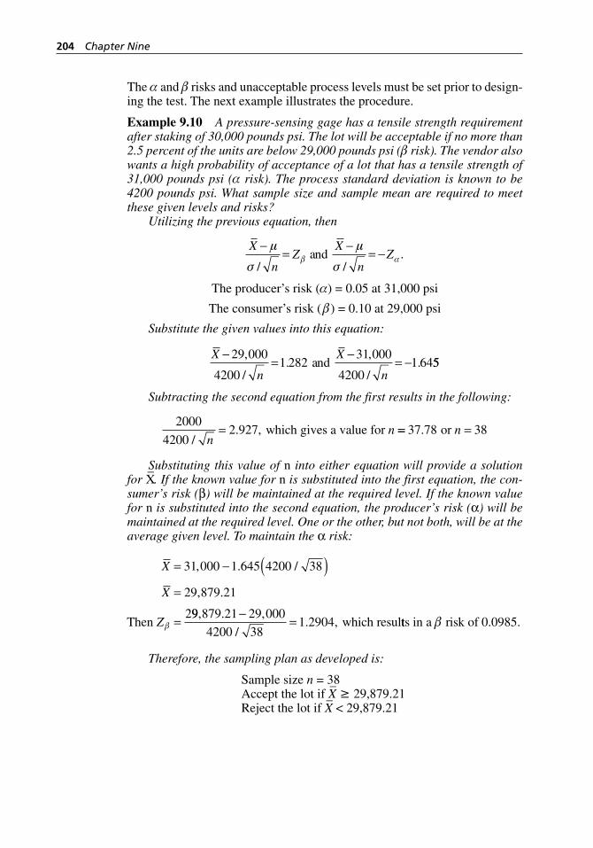
204 Chapter Nine
The α and β risks and unacceptable process levels must be set prior to design-ing the test. The next example illustrates the procedure.
Example 9.10 A pressure- sensing gage has a tensile strength requirement after staking of 30,000 pounds psi. The lot will be acceptable if no more than 2.5 percent of the units are below 29,000 pounds psi (β risk). The vendor also wants a high probability of acceptance of a lot that has a tensile strength of 31,000 pounds psi (α risk). The process standard deviation is known to be 4200 pounds psi. What sample size and sample mean are required to meet these given levels and risks?
Utilizing the previous equation, then
X
nZ
X
nZ
−=
−= −
µ
σ
µ
σβ α
/ /.and
The producer’s risk (α) = 0.05 at 31,000 psi
The consumer’s risk ( β) = 0.10 at 29,000 psi
Substitute the given values into this equation:
X
n
X
n
−=
−= −
29 000
42001 282
31 000
42001 64
,
/.
,
/.and 55
Subtracting the second equation from the first results in the following:
2000
42002 927
/. ,
nn= which gives a value for == =37 78 38. or n
Substituting this value of n into either equation will provide a solution for X
–. If the known value for n is substituted into the first equation, the con-
sumer’s risk (β) will be maintained at the required level. If the known value for n is substituted into the second equation, the producer’s risk (α) will be maintained at the required level. One or the other, but not both, will be at the average given level. To maintain the α risk:
X
X
Z
= − ( )=
=
31 000 1 645 4200 38
29 879 21
2
, . /
, .
Then β99 879 21 29 000
4200 381 2904
, . ,
/. ,
− = which resultts in a risk of 0.0985.β
Therefore, the sampling plan as developed is:
Sample size n = 38 Accept the lot if X
– ≥ 29,879.21
Reject the lot if X– < 29,879.21
H1277 ch09.indd 204H1277 ch09.indd 204 3/8/07 12:38:12 PM3/8/07 12:38:12 PM
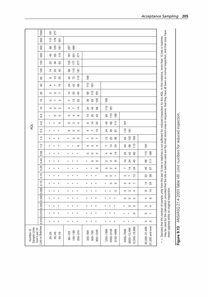
Acceptance Sampling 205
Num
ber
ofS
ampl
e U
nits
from
Las
t 10
Lots
or
Bat
ches
AQ
L
20–2
9
30–4
9
50–7
9
80–1
29
130–
199
200–
319
320–
499
500–
799
800–
1249
1250
–199
9
2000
–314
9
3150
–499
9
5000
–799
9
8000
–12,
499
12,5
00–1
9,99
9
20,0
00–3
1,49
9
31,5
00 a
nd o
ver
* * * * * * * * * * * *
* * * * * * * * * * * *
* * * * * * * * * * * *
* * * * * * * * * * * *
* * * * * * * * * * * 0
* * * * * * * * * * 0 0
* * * * * *
* * *
* * *
* * *
* * * 0 0
0 1* * 0
* 0 0 2 4
0 0 2 4 8
0 2 4 8 14
2 4 7 14 24
0 0 1 3 7 13 22 38
* * 0 0 2 4 7 14 24 40 67
* 0 0 2 4 8 14 24 40 68 111
* * * 0 0 2 4 8 14 25 42 69 115
186
181* * 0 0 2 4 7 14 24 40 68 110
* 0 0 1 3 7 13 22 38 63 105
169
* * *
* * *
* * *
* * *
* * *
* * *
0 0 2 4 7 14 24 40 67 110
181
* * 0 0 2 4 8 14 24 49 68 111
* 0 0 2 4 8 14 25 42 69 115
186
0 0 2 4 7 14 24 40 68 110
181
0 1 3 7 13 22 39 63 105
2 3 7 14 25 40 68 110
181
4 7 14 24 42 68 113
181
181
169
1898 13 25 42 72 115
14 22 40 68 115
181
22 36 63 105
177
277
40 63 110
181
301
471
68 105
181
297
490
115
178
301
181
277
0.01
50.
025
0.04
00.
065
0.10
0.15
0.25
0.40
0.65
1.0
1.5
2.5
4.0
6.5
1015
2540
6510
015
025
040
065
010
000.
010
= D
enot
es th
at th
e nu
mbe
r of
sam
ple
units
from
the
last
10
lots
or
batc
hes
is n
ot s
uffic
ient
for
redu
ced
insp
ectio
n fo
r th
is A
QL.
In th
is in
stan
ce, m
ore
than
10
lots
or
batc
hes
may
be
used
for
the
calc
ulat
ion,
pro
vide
d th
at th
e lo
ts o
r ba
tche
s us
ed a
re th
e m
ost r
ecen
t one
s in
seq
uenc
e, th
at th
ey h
ave
all b
een
on n
orm
al in
spec
tion,
and
that
non
e ha
ve
bee
n re
ject
ed w
hile
on
orig
inal
insp
ectio
n.
*
Fig
ure
9.1
3 A
NSI
/ASQ
Z1.
4-20
03 T
able
VIII
: Lim
it nu
mbe
rs f
or r
educ
ed in
spec
tion.
H1277 ch09.indd 205H1277 ch09.indd 205 3/8/07 12:38:12 PM3/8/07 12:38:12 PM
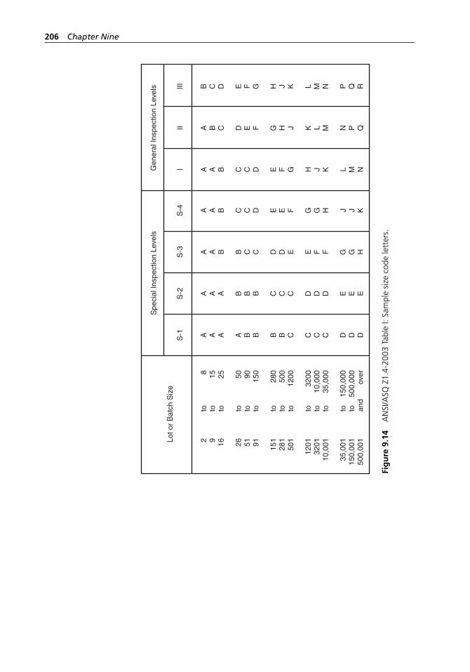
206 Chapter Nine
Lot o
r B
atch
Siz
e
2 9 16 26 51 91 151
281
501
1201
3201
10,0
01
35,0
0115
0,00
150
0,00
1
to to to to to to to to to to to to to to and
8 15 25 50 90 150
280
500
1200
3200
10,0
0035
,000
150,
000
500,
000
over
A A A A B B B B C C C C D D DS-1
A A A B B B C C C D D D E E ES-2
A A B B C C D D E E F F G G HS-3
A A B C C D E E F G G H J J KS-4
A A B C C D E F G H J K L M NI
A B C D E F G H J K L M N P QII
Spe
cial
Insp
ectio
n Le
vels
Gen
eral
Insp
ectio
n Le
vels B C D E F G H J K L M N P Q RIII
Fig
ure
9.1
4 A
NSI
/ASQ
Z1.
4-20
03 T
able
I: S
ampl
e si
ze c
ode
lett
ers.
H1277 ch09.indd 206H1277 ch09.indd 206 3/8/07 12:38:12 PM3/8/07 12:38:12 PM
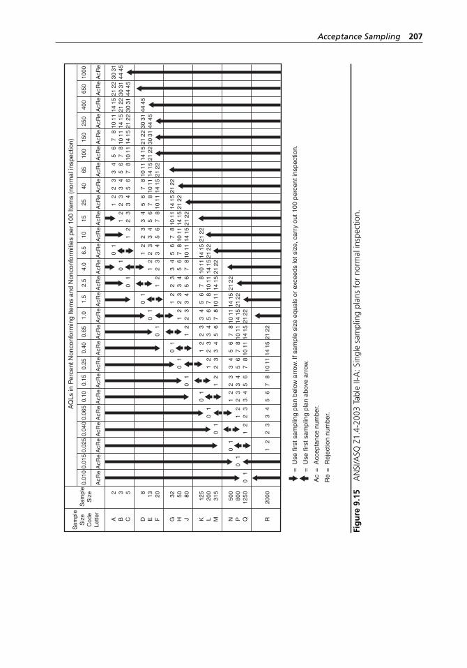
Acceptance Sampling 207
Sam
ple
Siz
eC
ode
Lette
r
Sam
ple
Siz
e
AQ
Ls in
Per
cent
Non
conf
orm
ing
Item
s an
d N
onco
nfor
miti
es p
er 1
00 It
ems
(nor
mal
insp
ectio
n)
A B C D E F G H J K L M N P Q R
2 3 5 8 13 20 32 50 80 125
200
315
500
800
1250
2000
11
1 2
1 2 3
1 2 3 4
1 2 3 4 6
1 2 3 4 6 8
1 2 3 4 6 8 11
1 2 3 4 6 8 11 15
1 2 3 4 6 8 11 15 22
1 2 3 4 6 8 11 15 22
1 2 3 4 6 8 11 15 22
1 2 3 4 6 8 11 15 22
1 2 3 4 6 8 11 15 22
1 2 3 4 6 8 11 15 22
2 3 4 6 8 11 15 22
2 3 4 6 8 11 15 22
2 3 4 6 8 11 15 22
3 4 6 8 11 15 22
4 6 8 11 15 22
6 8 11 15 22
8 11 15 22 31
11 15 22 31 45
15 22 31 45
22 31 45
31 45
00
Re
Ac
Re
Ac
Re
Ac
Re
Ac
Re
Ac
Re
Ac
Re
Ac
Re
Ac
Re
Ac
Re
Ac
Re
Ac
Re
Ac
Re
Ac
Re
Ac
Re
Ac
Re
Ac
Re
Ac
Re
Ac
Re
Ac
Re
Ac
Re
Ac
Re
Ac
Re
Ac
Re
Ac
Re
Ac
Re
Ac
0.01
50.
025
0.04
00.
065
0.10
0.15
0.25
0.40
0.65
1.0
1.5
2.5
4.0
6.5
1015
2540
6510
015
025
040
065
010
000.
010
0 1
0 1 2
0 1 2 3
0 1 2 3 5
0 1 2 3 5 7
0 1 2 3 5 7 10
0 1 2 3 5 7 10 14
0 1 2 3 5 7 10 14 21
0 1 2 3 5 7 10 14 21
0 1 2 3 5 7 10 14 21
0 1 2 3 5 7 10 14 21
0 1 2 3 5 7 10 14 21
0 1 2 3 5 7 10 14 21
1 2 3 5 7 10 14 21
1 2 3 5 7 10 14 21
1 2 3 5 7 10 14 21
2 3 5 7 10 14 21
3 5 7 10 14 21
5 7 10 14 21
7 10 14 21 30
10 14 21 30 44
14 21 30 44
21 30 44
30 44
= U
se fi
rst s
ampl
ing
plan
bel
ow a
rrow
. If s
ampl
e si
ze e
qual
s or
exc
eeds
lot s
ize,
car
ry o
ut 1
00 p
erce
nt in
spec
tion.
= U
se fi
rst s
ampl
ing
plan
abo
ve a
rrow
.
= A
ccep
tanc
e nu
mbe
r.
= R
ejec
tion
num
ber.
Ac
Re
Fig
ure
9.1
5 A
NSI
/ASQ
Z1.
4-20
03 T
able
II- A
: Sin
gle
sam
plin
g pl
ans
for
norm
al in
spec
tion.
H1277 ch09.indd 207H1277 ch09.indd 207 3/8/07 12:38:12 PM3/8/07 12:38:12 PM
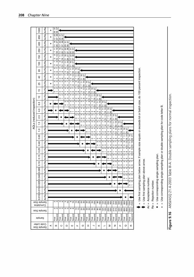
208 Chapter Nine
Sample SizeCode Letter
Sample
Sample Size
CumulativeSample Size
AQ
Ls (
redu
ced
insp
ectio
n)
A B C D E F G H J K L M N P Q R
Firs
tS
econ
dF
irst
Sec
ond
Firs
tS
econ
dF
irst
Sec
ond
Firs
tS
econ
dF
irst
Sec
ond
Firs
tS
econ
dF
irst
Sec
ond
Firs
tS
econ
dF
irst
Sec
ond
Firs
tS
econ
dF
irst
Sec
ond
Firs
tS
econ
dF
irst
Sec
ond
Firs
tS
econ
d
2 2 3 3 5 5 8 8 13 13 20 20 32 32 50 50 80 80 125
125
200
200
315
315
500
500
800
800
1250
1250
2 4 3 6 5 10 8 16 13 26 20 40 32 64 50 100 80 160
125
250
200
400
315
630
500
1000 80
016
0012
5025
000 1
2 2
0 1 0 3
2 2 3 4
0 1 0 3 1 4
2 2 3 4 4 5
0 1 0 3 1 4 2 6
2 2 3 4 4 5 5 7
0 1 0 3 1 4 2 6 3 8
2 2 3 4 4 5 5 7 7 9
0 1 0 3 1 4 2 6 3 8 5 12
2 2 3 4 4 5 5 7 7 9 9 13
0 1 0 3 1 4 2 6 3 8 5 12 7 18
2 2 3 4 4 5 5 7 7 9 9 13 11 1 9
0 1 0 3 1 4 2 6 3 8 5 12 7 18 11 26
2 2 3 4 4 5 5 7 7 9 9 13 11 19 16 27
0 1 0 3 1 4 2 6 3 8 5 12 7 18 11 26
2 2 3 4 4 5 5 7 7 9 9 13 11 19 16 27
0 1 0 3 1 4 2 6 3 8 5 12 7 18 11 26
2 2 3 4 4 5 5 7 7 9 9 13 11 19 16 27
0 1 0 3 1 4 2 6 3 8 5 12 7 18 11 26
2 2 3 4 4 5 5 7 7 9 9 13 11 19 16 27
0 1 0 3 1 4 2 6 3 8 5 12 7 18 11 26
2 2 3 4 4 5 5 7 7 9 9 13 11 19 16 27
0 1 0 3 1 4 2 6 3 8 5 12 7 18 11 26
2 2 3 4 4 5 5 7 7 9 9 13 11 19 16 27
0 1 0 3 1 4 2 6 3 8 5 12 7 18 11 26
2 2 3 4 4 5 5 7 7 9 9 13 11 19 16 27
0 1 0 3 1 4 2 6 3 8 5 12 7 18 11 26
2 2 3 4 4 5 5 7 7 9 9 13 11 19 16 27
0 3 1 4 2 6 3 8 5 12 7 18 11 26
3 4 4 5 5 7 7 9 9 13 11 19 16 27
1 4 2 6 3 8 5 12 7 18 11 26
4 5 5 7 7 9 9 13 11 19 16 27
2 6 3 8 5 12 7 18 11 26
5 7 7 9 9 13 11 19 16 27
3 8 5 12 7 18 11 26
7 9 9 13 11 19 16 27
5 12 7 18 11 26 17 37
9 13 11 19 16 27 22 38
7 18 11 26 17 37 25 56
11 19 16 27 22 38 31 57
11 26 17 37 25 56
16 27 22 38 31 57
17 37 25 56
22 38 31 57
25 5631 57
Re
Ac
Re
Ac
Re
Ac
Re
Ac
Re
Ac
Re
Ac
Re
Ac
Re
Ac
Re
Ac
Re
Ac
Re
Ac
Re
Ac
Re
Ac
Re
Ac
Re
Ac
Re
Ac
Re
Ac
Re
Ac
Re
Ac
Re
Ac
Re
Ac
Re
Ac
Re
Ac
Re
Ac
Re
Ac
Re
Ac
0.01
50.
025
0.04
00.
065
0.10
0.15
0.25
0.40
0.65
1.0
1.5
2.5
4.0
6.5
1015
2540
6510
015
025
040
065
010
000.
010
= U
se fi
rst s
ampl
ing
plan
bel
ow a
rrow
. If s
ampl
e si
ze e
qual
s or
exc
eeds
lot o
r ba
tch
size
, do
100
perc
ent i
nspe
ctio
n.
= U
se fi
rst s
ampl
ing
plan
abo
ve a
rrow
.
= A
ccep
tanc
e nu
mbe
r.
= R
ejec
tion
num
ber.
= U
se c
orre
spon
ding
sin
gle
sam
plin
g pl
an.
Ac
Re
= U
se c
orre
spon
ding
sin
gle
sam
plin
g pl
an o
r do
uble
sam
plin
g pl
an fo
r co
de le
tter
B.
+
++
++
++
++
+
Fig
ure
9.1
6 A
NSI
/ASQ
Z1.
4-20
03 T
able
III- A
: Dou
ble
sam
plin
g pl
ans
for
norm
al in
spec
tion.
H1277 ch09.indd 208H1277 ch09.indd 208 3/8/07 12:38:12 PM3/8/07 12:38:12 PM
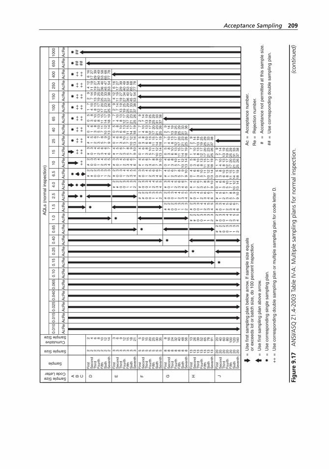
Acceptance Sampling 209
Sample SizeCode Letter
Sample
Sample Size
CumulativeSample Size
AQ
Ls (
norm
al in
spec
tion)
A CB D E F G H
Firs
tS
econ
dT
hird
Fou
rth
Fift
hS
ixth
Sev
enth
Firs
tS
econ
dT
hird
Fou
rth
Fift
hS
ixth
Sev
enth
Firs
tS
econ
dT
hird
Fou
rth
Fift
hS
ixth
Sev
enth
Firs
tS
econ
dT
hird
Fou
rth
Fift
hS
ixth
Sev
enth
Firs
tS
econ
dT
hird
Fou
rth
Fift
hS
ixth
Sev
enth
2 2 2 2 2 2 2 3 3 3 3 3 3 3 5 5 5 5 5 5 5 8 8 8 8 8 8 8 13 13 13 13 13 13 13
2 4 6 8 10 12 14
2 2 2 3 3 3 3
# # 0 0 1 1 2
2 3 3 4 4 5 5
# 0 0 1 2 3 4
3 3 4 5 6 6 7
# 0 1 2 3 4 6
4 5 6 7 8 9 10
# 1 2 3 5 7 9
4 6 8 10 11 12 14
0 1 3 5 7 10 13
5 8 10 13 15 17 19
0 3 6 8 11 14 18
7 10 13 17 20 23 26
1 4 8 12 17 21 25
9 14 19 25 29 33 38
2 7 13 19 25 31 37
12 19 27 34 40 47 54
4 11 19 27 36 45 53
16 27 39 49 58 68 78
6 17 29 40 53 65 772 2 2 3 3 3 3
# # 0 0 1 1 2
2 3 3 4 4 5 5
# 0 0 1 2 3 4
3 3 4 5 6 6 7
# 0 1 2 3 4 6
4 5 6 7 8 9 10
# 1 2 3 5 7 9
4 6 8 10 11 12 14
0 1 3 5 7 10 13
5 8 10 13 15 17 19
0 3 6 8 11 14 18
7 10 13 17 20 23 26
1 4 8 12 17 21 25
9 14 19 25 29 33 38
2 7 13 19 25 31 37
12 19 27 34 40 47 54
4 11 19 27 36 45 53
16 27 39 49 58 68 78
6 17 29 40 53 65 77
2 2 2 3 3 3 3
# # 0 0 1 1 2
2 3 3 4 4 5 5
# 0 0 1 2 3 4
3 3 4 5 6 6 7
# 0 1 2 3 4 6
4 5 6 7 8 9 10
# 1 2 3 5 7 9
4 6 8 10 11 12 14
0 1 3 5 7 10 13
5 8 10 13 15 17 19
0 3 6 8 11 14 18
7 10 13 17 20 23 26
1 4 8 12 17 21 25
9 14 19 25 29 33 38
2 7 13 19 25 31 372 2 2 3 3 3 3
# # 0 0 1 1 2
2 3 3 4 4 5 5
# 0 0 1 2 3 4
3 3 4 5 6 6 7
# 0 1 2 3 4 6
4 5 6 7 8 9 10
# 1 2 3 5 7 9
4 6 8 10 11 12 14
0 1 3 5 7 10 13
5 8 10 13 15 17 19
0 3 6 8 11 14 18
7 10 13 17 20 23 26
1 4 8 12 17 21 25
9 14 19 25 29 33 38
2 7 13 19 25 31 37
2 2 2 3 3 3 3
# # 0 0 1 1 2
2 3 3 4 4 5 5
# 0 0 1 2 3 4
3 3 4 5 6 6 7
# 0 1 2 3 4 6
4 5 6 7 8 9 10
# 1 2 3 5 7 9
4 6 8 10 11 12 14
0 1 3 5 7 10 13
5 8 10 13 15 17 19
0 3 6 8 11 14 18
7 10 13 17 20 23 26
1 4 8 12 17 21 25
9 14 19 25 29 33 38
2 7 13 19 25 31 37
2 2 2 3 3 3 3
# # 0 0 1 1 2
2 3 3 4 4 5 5
# 0 0 1 2 3 4
3 3 4 5 6 6 7
# 0 1 2 3 4 6
4 5 6 7 8 9 10
# 1 2 3 5 7 9
4 6 8 10 11 12 14
0 1 3 5 7 10 13
5 8 10 13 15 17 19
0 3 6 8 11 14 18
7 10 13 17 20 23 26
1 4 8 12 17 21 25
9 14 19 25 29 33 38
2 7 13 19 25 31 37
3 6 9 12 15 18 21 5 10 15 20 25 30 35 8 16 24 32 40 48 56 13 26 39 52 65 78 91
Re
Ac
Re
Ac
Re
Ac
Re
Ac
Re
Ac
Re
Ac
Re
Ac
Re
Ac
Re
Ac
Re
Ac
Re
Ac
Re
Ac
Re
Ac
Re
Ac
Re
Ac
Re
Ac
Re
Ac
Re
Ac
Re
Ac
Re
Ac
Re
Ac
Re
Ac
Re
Ac
Re
Ac
Re
Ac
Re
Ac
0.01
50.
025
0.04
00.
065
0.10
0.15
0.25
0.40
0.65
1.0
1.5
2.5
4.0
6.5
1015
2540
6510
015
025
040
065
010
000.
010
= U
se fi
rst s
ampl
ing
plan
bel
ow a
rrow
. If s
ampl
e si
ze e
qual
s
or
exce
eds
lot o
r ba
tch
size
, do
100
perc
ent i
nspe
ctio
n.
= U
se fi
rst s
ampl
ing
plan
abo
ve a
rrow
.
= U
se c
orre
spon
ding
sin
gle
sam
plin
g pl
an.
= U
se c
orre
spon
ding
dou
ble
sam
plin
g pl
an o
r m
ultip
le s
ampl
ing
plan
for
code
lette
r D
.
✸ ++
= A
ccep
tanc
e nu
mbe
r.
= R
ejec
tion
num
ber.
= A
ccep
tanc
e no
t per
mitt
ed a
t thi
s sa
mpl
e si
ze.
= U
se c
orre
spon
ding
dou
ble
sam
plin
g pl
an.
Ac
Re # ##
JF
irst
Sec
ond
Thi
rdF
ourt
hF
ifth
Six
thS
even
th
20 20 20 20 20 20 20
20 40 60 80 100
120
140
✸
✸
✸
✸
✸
✸
✸
✸✸
++
++
++
++
++
++
++
++
++
++
++
++
++
++
++
++
++
######
✸✸
✸✸
✸✸
✸✸
✸
Fig
ure
9.1
7 A
NSI
/ASQ
Z1.
4-20
03 T
able
IV- A
: Mul
tiple
sam
plin
g pl
ans
for
norm
al in
spec
tion.
(c
ontin
ued)
H1277 ch09.indd 209H1277 ch09.indd 209 3/8/07 12:38:13 PM3/8/07 12:38:13 PM
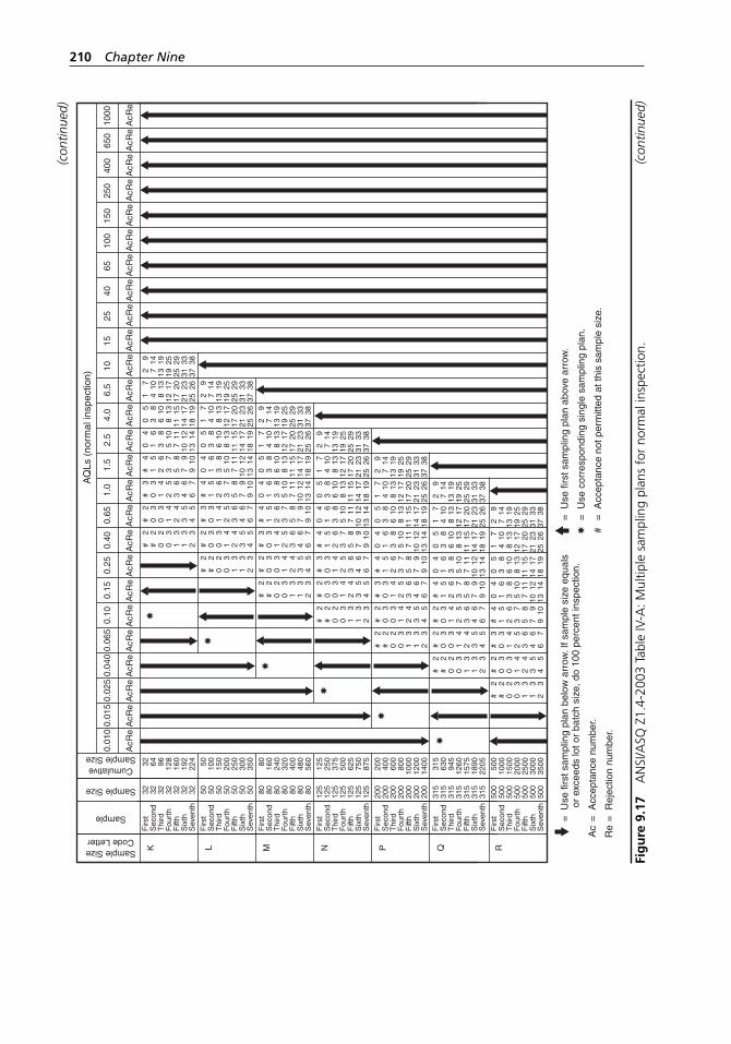
210 Chapter Nine
Sample SizeCode Letter
Sample
Sample Size
CumulativeSample Size
AQ
Ls (
norm
al in
spec
tion)
K L M N P Q
Firs
tS
econ
dT
hird
Fou
rth
Fift
hS
ixth
Sev
enth
Firs
tS
econ
dT
hird
Fou
rth
Fift
hS
ixth
Sev
enth
Firs
tS
econ
dT
hird
Fou
rth
Fift
hS
ixth
Sev
enth
Firs
tS
econ
dT
hird
Fou
rth
Fift
hS
ixth
Sev
enth
Firs
tS
econ
dT
hird
Fou
rth
Fift
hS
ixth
Sev
enth
50 50 50 50 50 50 50 80 80 80 80 80 80 80 125
125
125
125
125
125
125
200
200
200
200
200
200
200
315
315
315
315
315
315
315
50 100
150
200
250
300
350
Firs
tS
econ
dT
hird
Fou
rth
Fift
hS
ixth
Sev
enth
32 32 32 32 32 32 32
32 64 96 128
160
192
224
2 2 2 3 3 3 3
# # 0 0 1 1 2
2 3 3 4 4 5 5
# 0 0 1 2 3 4
3 3 4 5 6 6 7
# 0 1 2 3 4 6
4 5 6 7 8 9 10
# 1 2 3 5 7 9
4 6 8 10 11 12 14
0 1 3 5 7 10 13
5 8 10 13 15 17 19
0 3 6 8 11 14 18
7 10 13 17 20 23 26
1 4 8 12 17 21 25
9 14 19 25 29 33 38
2 7 13 19 25 31 37
2 2 2 3 3 3 3
# # 0 0 1 1 2
2 3 3 4 4 5 5
# 0 0 1 2 3 4
3 3 4 5 6 6 7
# 0 1 2 3 4 6
4 5 6 7 8 9 10
# 1 2 3 5 7 9
4 6 8 10 11 12 14
0 1 3 5 7 10 13
5 8 10 13 15 17 19
0 3 6 8 11 14 18
7 10 13 17 20 23 26
1 4 8 12 17 21 25
9 14 19 25 29 33 38
2 7 13 19 25 31 37
2 2 2 3 3 3 3
# # 0 0 1 1 2
2 3 3 4 4 5 5
# 0 0 1 2 3 4
3 3 4 5 6 6 7
# 0 1 2 3 4 6
4 5 6 7 8 9 10
# 1 2 3 5 7 9
4 6 8 10 11 12 14
0 1 3 5 7 10 13
5 8 10 13 15 17 19
0 3 6 8 11 14 18
7 10 13 17 20 23 26
1 4 8 12 17 21 25
9 14 19 25 29 33 38
2 7 13 19 25 31 37
2 2 2 3 3 3 3
# # 0 0 1 1 2
2 3 3 4 4 5 5
# 0 0 1 2 3 4
3 3 4 5 6 6 7
# 0 1 2 3 4 6
4 5 6 7 8 9 10
# 1 2 3 5 7 9
4 6 8 10 11 12 14
0 1 3 5 7 10 13
5 8 10 13 15 17 19
0 3 6 8 11 14 18
7 10 13 17 20 23 26
1 4 8 12 17 21 25
9 14 19 25 29 33 38
2 7 13 19 25 31 372 2 2 3 3 3 3
# # 0 0 1 1 2
2 3 3 4 4 5 5
# 0 0 1 2 3 4
3 3 4 5 6 6 7
# 0 1 2 3 4 6
4 5 6 7 8 9 10
# 1 2 3 5 7 9
4 6 8 10 11 12 14
0 1 3 5 7 10 13
5 8 10 13 15 17 19
0 3 6 8 11 14 18
7 10 13 17 20 23 26
1 4 8 12 17 21 25
9 14 19 25 29 33 38
2 7 13 19 25 31 37
2 2 2 3 3 3 3
# # 0 0 1 1 2
2 3 3 4 4 5 5
# 0 0 1 2 3 4
2 3 4 5 6 6 7
# 0 1 2 3 4 6
4 5 6 7 8 9 10
# 1 2 3 5 7 9
4 6 8 10 11 12 14
0 1 3 5 7 10 13
5 8 10 13 15 17 19
0 3 6 8 11 14 18
7 10 13 17 20 23 26
1 4 8 12 17 21 25
9 14 19 25 29 33 38
2 7 13 19 25 31 37
2 2 2 3 3 3 3
# # 0 0 1 1 2
2 3 3 4 4 5 5
# 0 0 1 2 3 4
3 3 4 5 6 6 7
# 0 1 2 3 4 6
4 5 6 7 8 9 10
# 1 2 3 5 7 9
4 6 8 10 11 12 14
0 1 3 5 7 10 13
5 8 10 13 15 17 19
0 3 6 8 11 14 18
7 10 13 17 20 23 26
1 4 8 12 17 21 25
9 14 19 25 29 33 38
2 7 13 19 25 31 37
80 160
240
320
400
480
560
125
250
375
500
625
750
875
200
400
600
800
1000
1200
1400 315
630
945
1260
1575
1890
2205
Re
Ac
Re
Ac
Re
Ac
Re
Ac
Re
Ac
Re
Ac
Re
Ac
Re
Ac
Re
Ac
Re
Ac
Re
Ac
Re
Ac
Re
Ac
Re
Ac
Re
Ac
Re
Ac
Re
Ac
Re
Ac
Re
Ac
Re
Ac
Re
Ac
Re
Ac
Re
Ac
Re
Ac
Re
Ac
Re
Ac
0.01
50.
025
0.04
00.
065
0.10
0.15
0.25
0.40
0.65
1.0
1.5
2.5
4.0
6.5
1015
2540
6510
015
025
040
065
010
000.
010
= U
se fi
rst s
ampl
ing
plan
bel
ow a
rrow
. If s
ampl
e si
ze e
qual
s
or
exce
eds
lot o
r ba
tch
size
, do
100
perc
ent i
nspe
ctio
n.
= A
ccep
tanc
e nu
mbe
r.
= R
ejec
tion
num
ber.
Ac
Re
= U
se fi
rst s
ampl
ing
plan
abo
ve a
rrow
.
= U
se c
orre
spon
ding
sin
gle
sam
plin
g pl
an.
= A
ccep
tanc
e no
t per
mitt
ed a
t thi
s sa
mpl
e si
ze.
✸ #
RF
irst
Sec
ond
Thi
rdF
ourt
hF
ifth
Six
thS
even
th
500
500
500
500
500
500
500
500
1000
1500
2000
2500
3000
3500
✸
✸
✸
✸
✸
✸
Fig
ure
9.1
7 A
NSI
/ASQ
Z1.
4-20
03 T
able
IV- A
: Mul
tiple
sam
plin
g pl
ans
for
norm
al in
spec
tion.
(c
ontin
ued)
(con
tinue
d)
H1277 ch09.indd 210H1277 ch09.indd 210 3/8/07 12:38:13 PM3/8/07 12:38:13 PM
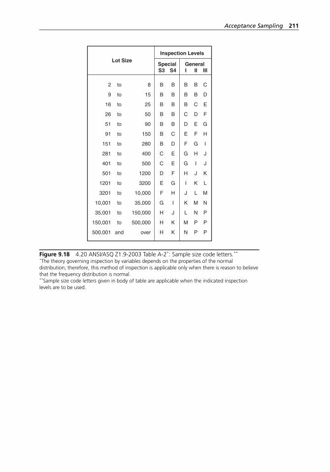
Acceptance Sampling 211
2
9
16
26
51
91
151
281
401
501
1201
3201
10,001
35,001
150,001
500,001
to
to
to
to
to
to
to
to
to
to
to
to
to
to
to
and
8
15
25
50
90
150
280
400
500
1200
3200
10,000
35,000
150,000
500,000
over
B
B
B
B
B
B
B
C
C
D
E
F
G
H
H
H
B
B
B
B
B
C
D
E
E
F
G
H
I
J
K
K
B
B
B
C
D
E
F
G
G
H
I
J
K
L
M
N
B
B
C
D
E
F
G
H
I
J
K
L
M
N
P
P
C
D
E
F
G
H
I
J
J
K
L
M
N
P
P
P
S3 S4 I II III
Lot SizeInspection Levels
Special General
Figure 9.18 4.20 ANSI/ASQ Z1.9-2003 Table A-2*: Sample size code letters.**
*The theory governing inspection by variables depends on the properties of the normal distribution; therefore, this method of inspection is applicable only when there is reason to believe that the frequency distribution is normal.**Sample size code letters given in body of table are applicable when the indicated inspection levels are to be used.
H1277 ch09.indd 211H1277 ch09.indd 211 3/8/07 12:38:14 PM3/8/07 12:38:14 PM
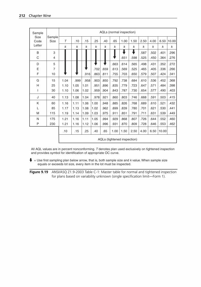
212 Chapter Nine
SampleSizeCodeLetter
SampleSize
AQLs (normal inspection)
AQLs (tightened inspection)
T
k
.10
k
.15
k
.25
k
.40
k
.65
k
1.00
k
1.50
k
2.50
k
4.00
k
6.50
k
10.00
k
B
C
D
E
F
G
H
I
K
L
M
N
P
J
3
4
5
7
10
15
25
30
60
85
115
175
230
40
.296
.276
.272
.266
.341
.368
.398
.403
.432
.441
.449
.460
.462
.415
.401
.364
.352
.336
.424
.452
.484
.490
.521
.530
.539
.552
.553
10.00
.503
.502
.450
.431
.405
.507
.536
.571
.577
.610
.621
.631
.644
.646
6.50
.591
.587
.525
.498
.465
.579
.610
.647
.654
.689
.701
.711
.726
.728
4.00
.668
.598
.565
.525
.650
.684
.723
.730
.768
.780
.791
.807
.809
2.50
.746
.651
.614
.569
.703
.738
.779
.787
.826
.839
.851
.868
.870
1.50
.803
.663
.613
.755
.792
.835
.843
.885
.899
.911
.929
.931
1.00
.860
.659
.811
.850
.896
.904
.948
.962
.975
.994
.996
.65
.921
.702
.863
.903
.951
.959
1.00
1.02
1.03
1.05
1.06
.40
.978
.916
.958
1.01
1.02
1.06
1.08
1.09
1.11
1.12
.25
1.04
.999
1.05
1.06
1.11
1.13
1.14
1.16
1.16
.15
1.08
1.04
1.10
1.10
1.16
1.17
1.19
1.21
1.21
.10
1.13
All AQL values are in percent nonconforming. T denotes plan used exclusively on tightened inspection and provides symbol for identification of appropriate OC curve.
= Use first sampling plan below arrow, that is, both sample size and k value. When sample size equals or exceeds lot size, every item in the lot must be inspected.
Figure 9.19 ANSI/ASQ Z1.9-2003 Table C-1: Master table for normal and tightened inspection for plans based on variability unknown (single specification limit—Form 1).
H1277 ch09.indd 212H1277 ch09.indd 212 3/8/07 12:38:14 PM3/8/07 12:38:14 PM
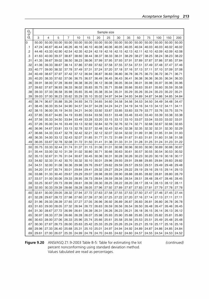
Acceptance Sampling 213
Sample sizeQUorQL
0 .1 .2 .3 .31.32.33.34.35.36.37.38.39
50.0047.2444.4641.6341.3541.0640.7740.4940.2039.9139.6239.3339.03
50.0046.6743.3340.0039.6739.3339.0038.6738.3338.0037.6737.3337.00
50.0046.4442.9039.3739.0238.6738.3237.9737.6237.2836.9336.5836.23
50.0046.2642.5438.8738.5038.1437.7837.4237.0636.6936.3335.9835.62
50.0046.1642.3538.6038.2337.8637.4937.1236.7536.3836.0235.6535.29
50.0046.1042.2438.4438.0637.6937.3136.9436.5736.2035.8335.4635.10
50.0046.0842.1938.3737.9937.6237.2436.8736.4936.1235.7535.3835.02
50.0046.0642.1638.3337.9537.5837.2036.8336.4536.0835.7135.3434.97
50.0046.0542.1538.3137.9337.5537.1836.8036.4336.0535.6835.3134.94
50.0046.0542.1338.2937.9137.5437.1636.7836.4136.0435.6635.2934.93
50.0046.0442.1138.2737.8937.5137.1336.7536.3836.0135.6335.2634.89
50.0046.0342.1038.2537.8737.4937.1136.7336.3635.9835.6135.2434.87
50.0046.0342.0938.2437.8637.4837.1036.7236.3535.9735.6035.2334.86
50.0046.0242.0938.2337.8537.4737.0936.7136.3435.9635.5935.2234.85
50.0046.0242.0838.2237.8437.4637.0836.7136.3335.9635.5835.2134.84
.40
.41
.42
.43
.44
.45
.46
.47
.48
.49
38.7438.4538.1537.8537.5637.2636.9636.6636.3536.05
36.6736.3336.0035.6735.3335.0034.6734.3334.0033.67
35.8835.5435.1934.8534.5034.1633.8133.4733.1232.78
35.2634.9034.5534.1933.8433.4933.1332.7832.4332.08
34.9334.5734.2133.8533.4933.1332.7832.4232.0731.72
34.7334.3734.0033.6433.2832.9232.5732.2131.8531.50
34.6534.2833.9233.5633.2032.8432.4832.1231.7731.41
34.6034.2433.8733.5133.1532.7932.4332.0731.7231.36
34.5834.2133.8533.4833.1232.7632.4032.0431.6931.33
34.5634.1933.8333.4633.1032.7432.3832.0231.6731.31
34.5334.1633.7933.4333.0732.7132.3531.9931.6331.28
34.5034.1333.7733.4033.0432.6832.3231.9631.6131.25
34.4934.1233.7633.3933.0332.6732.3131.9531.6031.24
34.4834.1133.7533.3833.0232.6632.3031.9431.5831.23
34.4734.1133.7433.3833.0132.6532.2931.9331.5831.22
.50
.51
.52
.53
.54
.55
.56
.57
.58
.59
35.7535.4435.1334.8234.5134.2033.8833.5733.2532.93
33.3333.0032.6732.3332.0031.6731.3331.0030.6730.33
32.4432.1031.7631.4231.0830.7430.4030.0629.7329.39
31.7431.3931.0430.7030.3630.0129.6729.3328.9928.66
31.3731.0230.6730.3229.9829.6429.2928.9528.6128.28
31.1530.8030.4530.1029.7629.4129.0728.7328.3928.05
31.0630.7130.3630.0129.6729.3228.9828.6428.3027.96
31.0130.6630.3129.9629.6229.2728.9328.5928.2527.92
30.9830.6330.2829.9329.5929.2428.9028.5628.2227.89
30.9630.6130.2629.9129.5729.2228.8828.5428.2027.87
30.9330.5730.2329.8829.5329.1928.8528.5128.1727.83
30.9030.5530.2029.8529.5129.1628.8228.4828.1427.81
30.8930.5430.1929.8429.4929.1528.8128.4728.1327.79
30.8830.5330.1829.8329.4829.1428.8028.4628.1227.78
30.8730.5230.1729.8229.4829.1328.7928.4528.1127.78
.60
.61
.62
.63
.64
.65
.66
.67
.68
.69
32.6132.2831.9631.6331.3030.9730.6330.3029.9629.61
30.0029.6729.3329.0028.6728.3328.0027.6727.3327.00
29.0528.7228.3928.0527.7227.3927.0626.7326.4026.07
28.3227.9827.6527.3226.9926.6626.3326.0025.6825.35
27.9427.6027.2726.9426.6126.2825.9625.6325.3124.99
27.7227.3927.0526.7226.3926.0725.7425.4225.1024.78
27.6327.3026.9626.6326.3125.9825.6625.3325.0124.70
27.5827.2526.9226.5926.2625.9325.6125.2924.9724.65
27.5527.2226.8926.5626.2325.9025.5825.2624.9424.62
27.5327.2026.8726.5426.2125.8825.5625.2424.9224.60
27.5027.1626.8326.5026.1825.8525.5325.2124.8924.57
27.4727.1426.8126.4826.1525.8325.5125.1924.8724.55
27.4627.1326.8026.4726.1425.8225.4925.1724.8624.54
27.4527.1126.7826.4626.1325.8125.4825.1624.8524.53
27.4427.1126.7826.4526.1225.8025.4825.1624.8424.52
3 4 5 7 10 15 20 25 30 35 50 75 100 150 200
Figure 9.20 ANSI/ASQ Z1.9-2003 Table B-5: Table for estimating the lot (continued)percent nonconforming using standard deviation method.
Values tabulated are read as percentages.
H1277 ch09.indd 213H1277 ch09.indd 213 3/8/07 12:38:14 PM3/8/07 12:38:14 PM
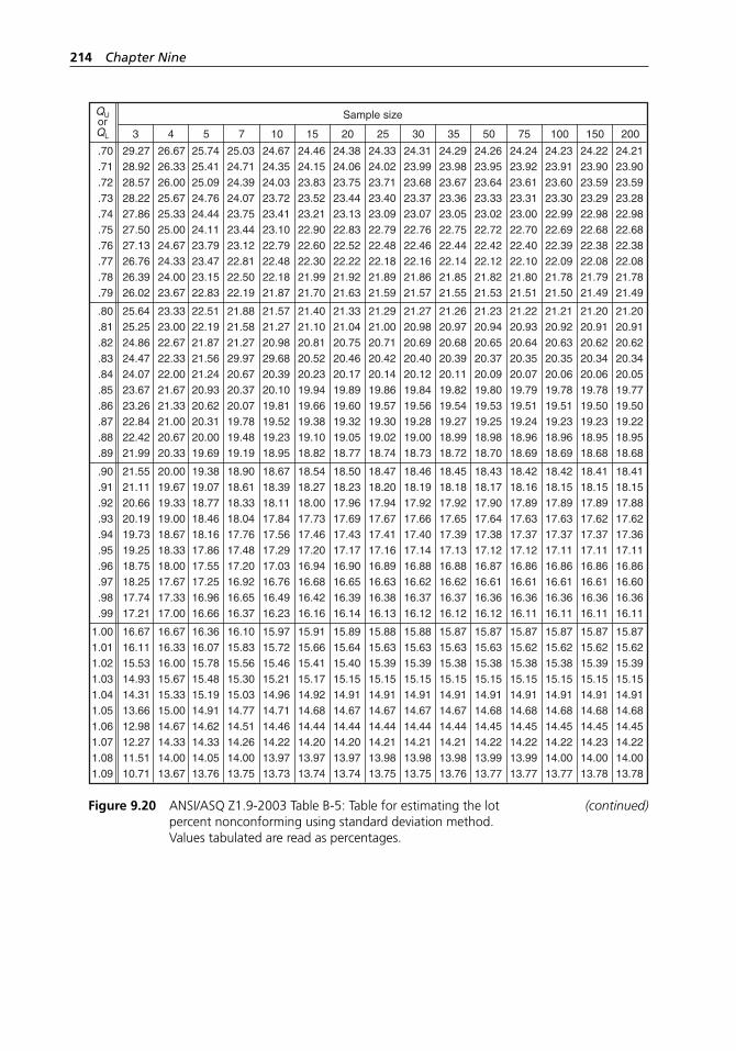
214 Chapter Nine
Sample sizeQUorQL
.70
.71
.72
.73
.74
.75
.76
.77
.78
.79
29.2728.9228.5728.2227.8627.5027.1326.7626.3926.02
26.6726.3326.0025.6725.3325.0024.6724.3324.0023.67
25.7425.4125.0924.7624.4424.1123.7923.4723.1522.83
25.0324.7124.3924.0723.7523.4423.1222.8122.5022.19
24.6724.3524.0323.7223.4123.1022.7922.4822.1821.87
24.4624.1523.8323.5223.2122.9022.6022.3021.9921.70
24.3824.0623.7523.4423.1322.8322.5222.2221.9221.63
24.3324.0223.7123.4023.0922.7922.4822.1821.8921.59
24.3123.9923.6823.3723.0722.7622.4622.1621.8621.57
24.2923.9823.6723.3623.0522.7522.4422.1421.8521.55
24.2623.9523.6423.3323.0222.7222.4222.1221.8221.53
24.2423.9223.6123.3123.0022.7022.4022.1021.8021.51
24.2323.9123.6023.3022.9922.6922.3922.0921.7821.50
24.2223.9023.5923.2922.9822.6822.3822.0821.7921.49
24.2123.9023.5923.2822.9822.6822.3822.0821.7821.49
.80
.81
.82
.83
.84
.85
.86
.87
.88
.89
25.6425.2524.8624.4724.0723.6723.2622.8422.4221.99
23.3323.0022.6722.3322.0021.6721.3321.0020.6720.33
22.5122.1921.8721.5621.2420.9320.6220.3120.0019.69
21.8821.5821.2729.9720.6720.3720.0719.7819.4819.19
21.5721.2720.9829.6820.3920.1019.8119.5219.2318.95
21.4021.1020.8120.5220.2319.9419.6619.3819.1018.82
21.3321.0420.7520.4620.1719.8919.6019.3219.0518.77
21.2921.0020.7120.4220.1419.8619.5719.3019.0218.74
21.2720.9820.6920.4020.1219.8419.5619.2819.0018.73
21.2620.9720.6820.3920.1119.8219.5419.2718.9918.72
21.2320.9420.6520.3720.0919.8019.5319.2518.9818.70
21.2220.9320.6420.3520.0719.7919.5119.2418.9618.69
21.2120.9220.6320.3520.0619.7819.5119.2318.9618.69
21.2020.9120.6220.3420.0619.7819.5019.2318.9518.68
21.2020.9120.6220.3420.0519.7719.5019.2218.9518.68
.90
.91
.92
.93
.94
.95
.96
.97
.98
.99
21.5521.1120.6620.1919.7319.2518.7518.2517.7417.21
20.0019.6719.3319.0018.6718.3318.0017.6717.3317.00
19.3819.0718.7718.4618.1617.8617.5517.2516.9616.66
18.9018.6118.3318.0417.7617.4817.2016.9216.6516.37
18.6718.3918.1117.8417.5617.2917.0316.7616.4916.23
18.5418.2718.0017.7317.4617.2016.9416.6816.4216.16
18.5018.2317.9617.6917.4317.1716.9016.6516.3916.14
18.4718.2017.9417.6717.4117.1616.8916.6316.3816.13
18.4618.1917.9217.6617.4017.1416.8816.6216.3716.12
18.4518.1817.9217.6517.3917.1316.8816.6216.3716.12
18.4318.1717.9017.6417.3817.1216.8716.6116.3616.12
18.4218.1617.8917.6317.3717.1216.8616.6116.3616.11
18.4218.1517.8917.6317.3717.1116.8616.6116.3616.11
18.4118.1517.8917.6217.3717.1116.8616.6116.3616.11
18.4118.1517.8817.6217.3617.1116.8616.6016.3616.11
1.001.011.021.031.041.051.061.071.081.09
16.6716.1115.5314.9314.3113.6612.9812.2711.5110.71
16.6716.3316.0015.6715.3315.0014.6714.3314.0013.67
16.3616.0715.7815.4815.1914.9114.6214.3314.0513.76
16.1015.8315.5615.3015.0314.7714.5114.2614.0013.75
15.9715.7215.4615.2114.9614.7114.4614.2213.9713.73
15.9115.6615.4115.1714.9214.6814.4414.2013.9713.74
15.8915.6415.4015.1514.9114.6714.4414.2013.9713.74
15.8815.6315.3915.1514.9114.6714.4414.2113.9813.75
15.8815.6315.3915.1514.9114.6714.4414.2113.9813.75
15.8715.6315.3815.1514.9114.6714.4414.2113.9813.76
15.8715.6315.3815.1514.9114.6814.4514.2213.9913.77
15.8715.6215.3815.1514.9114.6814.4514.2213.9913.77
15.8715.6215.3815.1514.9114.6814.4514.2214.0013.77
15.8715.6215.3915.1514.9114.6814.4514.2314.0013.78
15.8715.6215.3915.1514.9114.6814.4514.2214.0013.78
3 4 5 7 10 15 20 25 30 35 50 75 100 150 200
Figure 9.20 ANSI/ASQ Z1.9-2003 Table B-5: Table for estimating the lot (continued)percent nonconforming using standard deviation method.
Values tabulated are read as percentages.
H1277 ch09.indd 214H1277 ch09.indd 214 3/8/07 12:38:14 PM3/8/07 12:38:14 PM
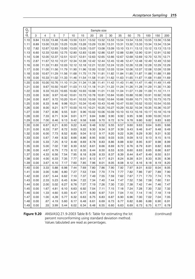
Acceptance Sampling 215
Sample sizeQUorQL
1.101.111.121.131.141.151.161.171.181.19
9.848.897.826.605.082.870.000.000.000.00
13.3313.0012.6712.3312.0011.6711.3311.0010.6710.33
13.4813.2012.9312.6512.3712.1011.8311.5611.2911.02
13.4913.2513.0012.7512.5112.2712.0311.7911.5611.33
13.5013.2613.0312.8012.5712.3412.1211.9011.6811.46
13.5113.2813.0512.8312.6112.3912.1811.9611.7511.54
13.5213.2913.0712.8512.6312.4212.2112.0011.7911.58
13.5213.3013.0812.8612.6512.4412.2212.0211.8111.61
13.5313.3113.0912.8712.6612.4512.2412.0311.8211.62
13.5413.3113.1012.8812.6712.4612.2512.0411.8411.63
13.5413.3213.1112.8912.6812.4712.2612.0611.8511.65
13.5513.3313.1212.9012.6912.4812.2812.0711.8711.67
13.5513.3413.1212.9112.7012.4912.2812.0811.8811.68
13.5613.3413.1312.9112.7012.4912.2912.0911.8811.69
13.5613.3413.1312.9212.7112.5012.2912.0911.8911.69
1.201.211.221.231.241.251.261.271.281.29
0.000.000.000.000.000.000.000.000.000.00
10.00 9.67 9.33 9.008.678.338.007.677.337.00
10.7610.5010.239.979.729.469.218.968.718.46
11.1010.8710.6510.4210.209.989.779.559.349.13
11.2411.0310.8210.6110.4110.2110.009.819.619.42
11.3411.1310.9310.7310.5310.3410.159.969.779.58
11.3811.1810.9810.7810.5910.4010.2110.02
9.849.66
11.4111.2111.0110.8110.6210.4310.2510.06
9.889.70
11.4211.2211.0310.8410.6410.4610.2710.09
9.909.72
11.4311.2411.0410.8510.6610.4710.2910.10
9.929.74
11.4611.2611.0710.8810.6910.5010.3210.13
9.959.78
11.4711.2811.0910.9010.7110.5210.3410.16
9.989.80
11.4811.2911.0910.9110.7210.5310.3510.17
9.999.82
11.4911.3011.1010.9210.7310.5410.3610.1810.00
9.83
11.4911.3011.1110.9210.7310.5510.3710.1910.01
9.83
1.301.311.321.331.341.351.361.371.381.39
0.000.000.000.000.000.000.000.000.000.00
6.676.336.005.675.335.004.674.334.003.67
8.217.977.737.497.257.026.796.566.336.10
8.938.728.528.328.127.927.737.547.357.17
9.229.038.858.668.488.308.127.957.777.60
9.409.229.048.868.698.528.358.188.017.85
9.489.309.128.958.788.618.448.288.127.96
9.529.349.179.008.838.668.508.338.178.01
9.559.379.209.038.868.698.538.378.218.05
9.579.399.229.058.888.728.558.398.248.08
9.609.439.269.098.928.768.608.448.288.12
9.639.469.299.128.958.798.638.478.318.16
9.649.479.309.138.978.818.658.498.338.18
9.659.489.319.158.988.828.668.508.358.19
9.669.499.329.158.998.838.678.518.368.20
1.401.411.421.431.441.451.461.471.481.49
0.000.000.000.000.000.000.000.000.000.00
3.333.002.672.332.001.671.331.00.67.33
5.885.665.445.235.024.814.604,394.193.99
6.986.806.626.456.276.105.935.775.605.44
7.447.277.106.946.786.636.476.326.176.02
7.697.537.377.227.076.926.776.636.486.34
7.807.647.497.347.197.046.906.756.616.48
7.867.707.557.407.267.116.976.836.696.55
7.907.747.597.447.307.157.016.876.736.60
7.927.777.627.477.337.187.046.906.776.63
7.977.827.677.527.387.247.106.966.826.69
8.017.867.717.567.427.287.147.006.866.73
8.027.877.737.587.447.307.167.026.886.75
8.047.897.747.607.467.327.187.046.906.77
8.057.907.757.617.477.327.197.056.916.78
3 4 5 7 10 15 20 25 30 35 50 75 100 150 200
Figure 9.20 ANSI/ASQ Z1.9-2003 Table B-5: Table for estimating the lot (continued)percent nonconforming using standard deviation method.
Values tabulated are read as percentages.
H1277 ch09.indd 215H1277 ch09.indd 215 3/8/07 12:38:14 PM3/8/07 12:38:14 PM
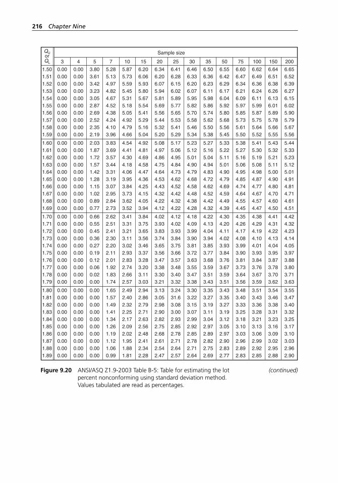
216 Chapter Nine
Sample sizeQUorQL
1.501.511.521.531.541.551.561.571.581.59
0.000.000.000.000.000.000.000.000.000.00
0.000.000.000.000.000.000.000.000.000.00
3.803.613.423.233.052.872.692.522.352.19
5.285.134.974.824.674.524.384.244.103.96
5.875.735.595.455.315.185.054.924.794.66
6.206.065.935.805.675.545.415.295.165.04
6.346.206.075.945.815.695.565.445.325.20
6.416.286.156.025.895.775.655.535.415.29
6.466.336.206.075.955.825.705.585.465.34
6.506.366.236.115.985.865.745.625.505.38
6.556.426.296.176.045.925.805.685.565.45
6.606.476.346.216.095.975.855.735.615.50
6.626.496.366.246.115.995.875.755.645.52
6.646.516.386.266.136.015.895.785.665.55
6.656.526.396.276.156.025.905.795.675.56
1.601.611.621.631.641.651.661.671.681.69
0.000.000.000.000.000.000.000.000.000.00
0.000.000.000.000.000.000.000.000.000.00
2.031.871.721.571.421.281.151.020.890.77
3.833.693.573.443.313.193.072.952.842.73
4.544.414.304.184.063.953.843.733.623.52
4.924.814.694.584.474.364.254.154.053.94
5.084.974.864.754.644.534.434.324.224.12
5.175.064.954.844.734.624.524.424.324.22
5.235.125.014.904.794.684.584.484.384.28
5.275.165.044.944.834.724.624.524.424.32
5.335.225.115.014.904.794.694.594.494.39
5.385.275.165.064.954.854.744.644.554.45
5.415.305.195.084.984.874.774.674.574.47
5.435.325.215.115.004.904.804.704.604.50
5.445.335.235.125.014.914.814.714.614.51
1.701.711.721.731.741.751.761.771.781.79
0.000.000.000.000.000.000.000.000.000.00
0.000.000.000.000.000.000.000.000.000.00
0.660.550.450.360.270.190.120.060.020.00
2.622.512.412.302.202.112.011.921.831.74
3.413.313.213.113.022.932.832.742.662.57
3.843.753.653.563.463.373.283.203.113.03
4.023.933.833.743.653.563.473.383.303.21
4.124.023.933.843.753.663.573.483.403.32
4.184.093.993.903.813.723.633.553.473.38
4.224.134.043.943.853.773.683.593.513.43
4.304.204.114.023.933.843.763.673.593.51
4.354.264.174.083.993.903.813.733.643.56
4.384.294.194.104.013.933.843.763.673.59
4.414.314.224.134.043.953.873.783.703.62
4.424.324.234.144.053.973.883.803.713.63
1.801.811.821.831.841.851.861.871.881.89
0.000.000.000.000.000.000.000.000.000.00
0.000.000.000.000.000.000.000.000.000.00
0.000.000.000.000.000.000.000.000.000.00
1.651.571.491.411.341.261.191.121.060.99
2.492.402.322.252.172.092.021.951.881.81
2.942.862.792.712.632.562.482.412.342.28
3.133.052.982.902.822.752.682.612.542.47
3.2431.63.083.002.932.852.782.712.642.57
3.303.223.153.072.992.922.852.782.712.64
3.353.273.193.113.042.972.892.822.752.69
3.433.353.273.193.123.052.972.902.832.77
3.483.403.333.253.183.103.032.962.892.83
3.513.433.363.283.213.133.062.992.922.85
3.543.463.383.313.233.163.093.022.952.88
3.553.473.403.323.253.173.103.032.962.90
3 4 5 7 10 15 20 25 30 35 50 75 100 150 200
Figure 9.20 ANSI/ASQ Z1.9-2003 Table B-5: Table for estimating the lot (continued)percent nonconforming using standard deviation method.
Values tabulated are read as percentages.
H1277 ch09.indd 216H1277 ch09.indd 216 3/8/07 12:38:14 PM3/8/07 12:38:14 PM
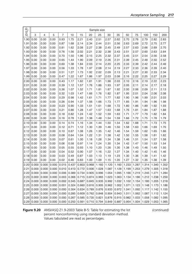
Acceptance Sampling 217
Sample sizeQUorQL
1.901.911.921.931.941.951.961.971.981.99
0.00 0.00 0.00 0.00 0.00 0.00 0.00 0.00 0.00 0.00
0.00 0.00 0.00 0.00 0.00 0.00 0.00 0.00 0.00 0.00
0.00 0.00 0.00 0.00 0.00 0.00 0.00 0.00 0.00 0.00
0.93 0.87 0.81 0.76 0.70 0.65 0.60 0.56 0.51 0.47
1.75 1.68 1.62 1.56 1.50 1.44 1.38 1.33 1.27 1.22
2.21 2.14 2.08 2.02 1.96 1.90 1.84 1.78 1.73 1.67
2.40 2.34 2.27 2.21 2.15 2.09 2.03 1.97 1.92 1.86
2.51 2.44 2.38 2.32 2.25 2.19 2.14 2.08 2.02 1.97
2.57 2.51 2.45 2.38 2.32 2.26 2.20 2.14 2.09 2.03
2.62 2.56 2.49 2.43 2.37 2.31 2.25 2.19 2.13 2.08
2.70 2.63 2.57 2.51 2.45 2.39 2.33 2.27 2.21 2.16
2.76 2.69 2.63 2.57 2.51 2.45 2.39 2.33 2.27 2.22
2.79 2.72 2.66 2.60 2.54 2.48 2.42 2.36 2.30 2.25
2.82 2.75 2.69 2.63 2.56 2.50 2.44 2.39 2.33 2.27
2.83 2.77 2.70 2.64 2.58 2.52 2.46 2.40 2.34 2.29
2.002.012.022.032.042.052.062.072.082.09
0.00 0.00 0.00 0.00 0.00 0.00 0.00 0.00 0.00 0.00
0.00 0.00 0.00 0.00 0.00 0.00 0.00 0.00 0.00 0.00
0.00 0.00 0.00 0.00 0.00 0.00 0.00 0.00 0.00 0.00
0.43 0.39 0.36 0.32 0.29 0.26 0.23 0.21 0.18 0.16
1.17 1.12 1.07 1.03 0.98 0.94 0.90 0.86 0.82 0.78
1.62 1.57 1.52 1.47 1.42 1.37 1.33 1.28 1.24 1.20
1.81 1.76 1.71 1.66 1.61 1.56 1.51 1.47 1.42 1.38
1.91 1.86 1.81 1.76 1.71 1.66 1.61 1.57 1.52 1.48
1.98 1.93 1.87 1.82 1.77 1.73 1.68 1.63 1.59 1.54
2.03 1.97 1.92 1.87 1.82 1.77 1.72 1.68 1.63 1.59
2.10 2.05 2.00 1.95 1.90 1.85 1.80 1.76 1.71 1.66
2.16 2.11 2.06 2.01 1.96 1.91 1.86 1.81 1.77 1.72
2.19 2.14 2.09 2.04 1.99 1.94 1.89 1.84 1.79 1.75
2.22 2.17 2.11 2.06 2.01 1.96 1.92 1.87 1.82 1.78
2.23 2.18 2.13 2.08 2.03 1.98 1.93 1.88 1.84 1.79
2.102.112.122.132.142.152.162.172.182.19
0.00 0.00 0.00 0.00 0.00 0.00 0.00 0.00 0.00 0.00
0.00 0.00 0.00 0.00 0.00 0.00 0.00 0.00 0.00 0.00
0.00 0.00 0.00 0.00 0.00 0.00 0.00 0.00 0.00 0.00
0.14 0.12 0.10 0.08 0.07 0.06 0.05 0.04 0.03 0.02
0.74 0.71 0.67 0.64 0.61 0.58 0.55 0.52 0.49 0.46
1.16 1.12 1.08 1.04 1.00 0.97 0.93 0.90 0.87 0.83
1.34 1.30 1.26 1.22 1.18 1.14 1.10 1.07 1.03 1.00
1.44 1.39 1.35 1.31 1.28 1.24 1.20 1.16 1.13 1.09
1.50 1.46 1.42 1.38 1.34 1.30 1.26 1.22 1.19 1.15
1.54 1.50 1.46 1.42 1.38 1.34 1.30 1.27 1.23 1.20
1.62 1.58 1.54 1.50 1.46 1.42 1.38 1.34 1.30 1.27
1.68 1.63 1.59 1.55 1.51 1.47 1.43 1.40 1.36 1.32
1.71 1.66 1.62 1.58 1.54 1.50 1.46 1.42 1.39 1.35
1.73 1.69 1.65 1.61 1.57 1.53 1.49 1.45 1.41 1.38
1.75 1.70 1.66 1.62 1.58 1.54 1.50 1.46 1.42 1.39
2.202.212.222.232.242.252.262.272.282.29
0.0000.0000.0000.0000.0000.0000.0000.0000.0000.000
0.0000.0000.0000.0000.0000.0000.0000.0000.0000.000
0.0000.0000.0000.0000.0000.0000.0000.0000.0000.000
0.0150.0100.0060.0030.0020.0010.0000.0000.0000.000
0.4370.4130.3890.3660.3450.3240.3040.2850.2670.250
0.8030.7720.7340.7150.6870.6600.6340.6090.5850.561
0.9680.9360.9050.8740.8450.8160.7890.7620.7350.710
1.1601.0280.9960.9650.9350.9050.8760.8480.8210.794
1.1201.0871.0541.0230.9920.9620.9330.9040.8760.849
1.1601.1281.0951.0631.0321.0020.9720.9430.9150.887
1.2331.1991.1661.1341.1021.0711.0411.0110.9820.954
1.2871.2531.2191.1861.1541.1231.0921.0621.0331.004
1.3141.2791.2451.2121.1801.1481.1171.0871.0581.029
1.3401.3051.2711.2381.2051.1731.1421.1121.0821.053
1.3521.3181.2841.2501.2181.1861.1551.1241.0951.065
3 4 5 7 10 15 20 25 30 35 50 75 100 150 200
Figure 9.20 ANSI/ASQ Z1.9-2003 Table B-5: Table for estimating the lot (continued)percent nonconforming using standard deviation method.
Values tabulated are read as percentages.
H1277 ch09.indd 217H1277 ch09.indd 217 3/8/07 12:38:14 PM3/8/07 12:38:14 PM
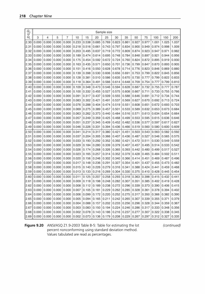
218 Chapter Nine
Sample sizeQUorQL
2.302.312.322.332.342.352.362.372.382.39
0.0000.0000.0000.0000.0000.0000.0000.0000.0000.000
0.0000.0000.0000.0000.0000.0000.0000.0000.0000.000
0.0000.0000.0000.0000.0000.0000.0000.0000.0000.000
0.0000.0000.0000.0000.0000.0000.0000.0000.0000.000
0.2330.2180.2030.1890.1750.1630.1510.1390.1280.118
0.5380.5160.4950.4740.4540.4350.4160.3980.3810.364
0.6850.6610.6370.6140.5920.5710.5500.5300.5100.491
0.7690.7430.7190.6950.6720.6500.6280.6060.5860.566
0.8230.7970.7720.7480.7240.7010.6780.6560.6350.614
0.8610.8340.8090.7840.7600.7360.7140.6910.6700.648
0.9270.9000.8740.8480.8240.7990.7760.7530.7300.709
0.9770.9490.9230.8970.8720.8470.8230.7990.7770.754
1.0010.9740.9470.9210.8950.8700.8460.8220.7990.777
1.0250.9980.9710.9440.9190.8930.8690.8450.8220.799
1.0371.0090.9820.9560.9300.9050.8800.8560.8330.810
2.402.412.422.432.442.452.462.472.482.49
0.0000.0000.0000.0000.0000.0000.0000.0000.0000.000
0.0000.0000.0000.0000.0000.0000.0000.0000.0000.000
0.0000.0000.0000.0000.0000.0000.0000.0000.0000.000
0.0000.0000.0000.0000.0000.0000.0000.0000.0000.000
0.1090.1000.0910.0830.0760.0690.0630.0570.0510.046
0.3480.3320.3170.3020.2880.2750.2620.2490.2370.226
0.4730.4550.4370.4210.4040.3890.3730.3590.3450.331
0.5460.5270.5090.4910.4740.4570.4400.4250.4090.394
0.5940.5750.5550.5370.5190.5010.4840.4680.4520.436
0.6280.6080.5880.5690.5510.5330.5160.4990.4820.466
0.6870.6670.6460.6270.6080.5890.5710.5530.5360.519
0.7320.7110.6910.6700.6510.6320.6130.5950.5770.560
0.7550.7330.7120.6920.6720.6530.6340.6150.5970.580
0.7770.7550.7340.7130.6930.6730.6540.6360.6170.600
0.7870.7660.7440.7240.7030.6840.6640.6460.6270.609
2.502.512.522.532.542.552.562.572.582.59
0.0000.0000.0000.0000.0000.0000.0000.0000.0000.000
0.0000.0000.0000.0000.0000.0000.0000.0000.0000.000
0.0000.0000.0000.0000.0000.0000.0000.0000.0000.000
0.0000.0000.0000.0000.0000.0000.0000.0000.0000.000
0.0410.0370.0330.0290.0260.0230.0200.0170.0150.013
0.2140.2040.1930.1840.1740.1650.1560.1480.1400.133
0.3170.3050.2920.2800.2680.2570.2460.2360.2260.216
0.3800.3660.3520.3390.3260.3140.3020.2910.2790.269
0.4210.4070.3920.3790.3650.3520.3400.3270.3160.304
0.4510.4360.4210.4070.3930.3790.3660.3540.3410.330
0.5030.4870.4720.4570.4420.4280.4140.4010.3880.375
0.5430.5270.5110.4950.4800.4650.4510.4370.4240.410
0.5630.5460.5300.5140.4990.4840.4690.4550.4410.428
0.5820.5650.5490.5330.5170.5020.4870.4730.4590.445
0.5920.5750.5590.5420.5270.5110.4960.4820.4680.454
2.602.612.622.632.642.652.662.672.682.69
0.0000.0000.0000.0000.0000.0000.0000.0000.0000.000
0.0000.0000.0000.0000.0000.0000.0000.0000.0000.000
0.0000.0000.0000.0000.0000.0000.0000.0000.0000.000
0.0000.0000.0000.0000.0000.0000.0000.0000.0000.000
0.0110.0090.0080.0070.0060.0050.0040.0030.0020.002
0.1250.1180.1120.1050.0990.0940.0880.0830.0780.073
0.2070.1980.1890.1810.1720.1650.1570.1500.1430.136
0.2580.2480.2380.2290.2200.2110.2020.1940.1860.179
0.2930.2820.2720.2620.2520.2420.2330.2240.2160.208
0.3180.3070.2960.2850.2750.2650.2560.2460.2370.229
0.3630.3510.3390.3280.3170.3070.2960.2860.2770.267
0.3980.3850.3730.3610.3500.3390.3280.3170.3070.297
0.4150.4020.3900.3780.3660.3550.3440.3330.3220.312
0.4320.4190.4060.3940.3820.3710.3590.3480.3380.327
0.4410.4280.4150.4020.3900.3790.3670.3560.3450.335
3 4 5 7 10 15 20 25 30 35 50 75 100 150 200
Figure 9.20 ANSI/ASQ Z1.9-2003 Table B-5: Table for estimating the lot (continued)percent nonconforming using standard deviation method.
Values tabulated are read as percentages.
H1277 ch09.indd 218H1277 ch09.indd 218 3/8/07 12:38:14 PM3/8/07 12:38:14 PM
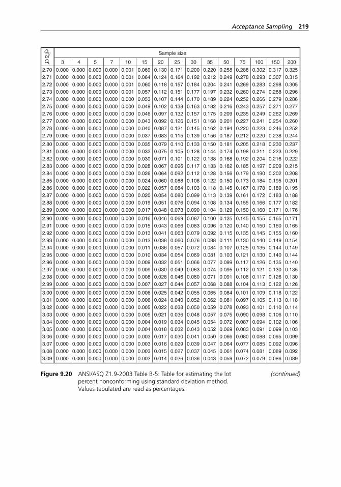
Acceptance Sampling 219
Sample sizeQUorQL
2.702.712.722.732.742.752.762.772.782.79
0.0000.0000.0000.0000.0000.0000.0000.0000.0000.000
0.0000.0000.0000.0000.0000.0000.0000.0000.0000.000
0.0000.0000.0000.0000.0000.0000.0000.0000.0000.000
0.0000.0000.0000.0000.0000.0000.0000.0000.0000.000
0.0010.0010.0010.0010.0000.0000.0000.0000.0000.000
0.0690.0640.0600.0570.0530.0490.0460.0430.0400.037
0.1300.1240.1180.1120.1070.1020.0970.0920.0870.083
0.1710.1640.1570.1510.1440.1380.1320.1260.1210.115
0.2000.1920.1840.1770.1700.1630.1570.1510.1450.139
0.2200.2120.2040.1970.1890.1820.1750.1680.1620.156
0.2580.2490.2410.2320.2240.2160.2090.2010.1940.187
0.2880.2780.2690.2600.2520.2430.2350.2270.2200.212
0.3020.2930.2830.2740.2660.2570.2490.2410.2230.220
0.3170.3070.2980.2880.2790.2710.2620.2540.2460.238
0.3250.3150.3050.2960.2860.2770.2690.2600.2520.244
2.802.812.822.832.842.852.862.872.882.89
0.0000.0000.0000.0000.0000.0000.0000.0000.0000.000
0.0000.0000.0000.0000.0000.0000.0000.0000.0000.000
0.0000.0000.0000.0000.0000.0000.0000.0000.0000.000
0.0000.0000.0000.0000.0000.0000.0000.0000.0000.000
0.0000.0000.0000.0000.0000.0000.0000.0000.0000.000
0.0350.0320.0300.0280.0260.0240.0220.0200.0190.017
0.0790.0750.0710.0670.0640.0600.0570.0540.0510.048
0.1100.1050.1010.0960.0920.0880.0840.0800.0760.073
0.1330.1280.1220.1170.1120.1080.1030.0990.0940.090
0.1500.1440.1380.1330.1280.1220.1180.1130.1080.104
0.1810.1740.1680.1620.1560.1500.1450.1390.1340.129
0.2050.1980.1920.1850.1790.1730.1670.1610.1550.150
0.2180.2110.2040.1970.1900.1840.1780.1720.1660.160
0.2300.2230.2160.2090.2020.1950.1890.1830.1770.171
0.2370.2290.2220.2150.2080.2010.1950.1880.1820.176
2.902.912.922.932.942.952.962.972.982.99
0.0000.0000.0000.0000.0000.0000.0000.0000.0000.000
0.0000.0000.0000.0000.0000.0000.0000.0000.0000.000
0.0000.0000.0000.0000.0000.0000.0000.0000.0000.000
0.0000.0000.0000.0000.0000.0000.0000.0000.0000.000
0.0000.0000.0000.0000.0000.0000.0000.0000.0000.000
0.0160.0150.0130.0120.0110.0100.0090.0090.0080.007
0.0460.0430.0410.0380.0360.0340.0320.0300.0280.027
0.0690.0660.0630.0600.0570.0540.0510.0490.0460.044
0.0870.0830.0790.0760.0720.0690.0660.0630.0600.057
0.1000.0960.0920.0880.0840.0810.0770.0740.0710.068
0.1250.1200.1150.1110.1070.1030.0990.0950.0910.088
0.1450.1400.1350.1300.1250.1210.1170.1120.1080.104
0.1550.1500.1450.1400.1350.1300.1260.1210.1170.113
0.1650.1600.1550.1490.1440.1400.1350.1300.1260.122
0.1710.1650.1600.1540.1490.1440.1400.1350.1300.126
3.003.013.023.033.043.053.063.073.083.09
0.0000.0000.0000.0000.0000.0000.0000.0000.0000.000
0.0000.0000.0000.0000.0000.0000.0000.0000.0000.000
0.0000.0000.0000.0000.0000.0000.0000.0000.0000.000
0.0000.0000.0000.0000.0000.0000.0000.0000.0000.000
0.0000.0000.0000.0000.0000.0000.0000.0000.0000.000
0.0060.0060.0050.0050.0040.0040.0030.0030.0030.002
0.0250.0240.0220.0210.0190.0180.0170.0160.0150.014
0.0420.0400.0380.0360.0340.0320.0300.0290.0270.026
0.0550.0520.0500.0480.0450.0430.0410.0390.0370.036
0.0650.0620.0590.0570.0540.0520.0500.0470.0450.043
0.0840.0810.0780.0750.0720.0690.0660.0640.0610.059
0.1010.0970.0930.0900.0870.0830.0800.0770.0740.072
0.1090.1050.1010.0980.0940.0910.0880.0850.0810.079
0.1180.1130.1100.1060.1020.0990.0950.0920.0890.086
0.1220.1180.1140.1100.1060.1030.0990.0960.0920.089
3 4 5 7 10 15 20 25 30 35 50 75 100 150 200
Figure 9.20 ANSI/ASQ Z1.9-2003 Table B-5: Table for estimating the lot (continued)percent nonconforming using standard deviation method.
Values tabulated are read as percentages.
H1277 ch09.indd 219H1277 ch09.indd 219 3/8/07 12:38:15 PM3/8/07 12:38:15 PM
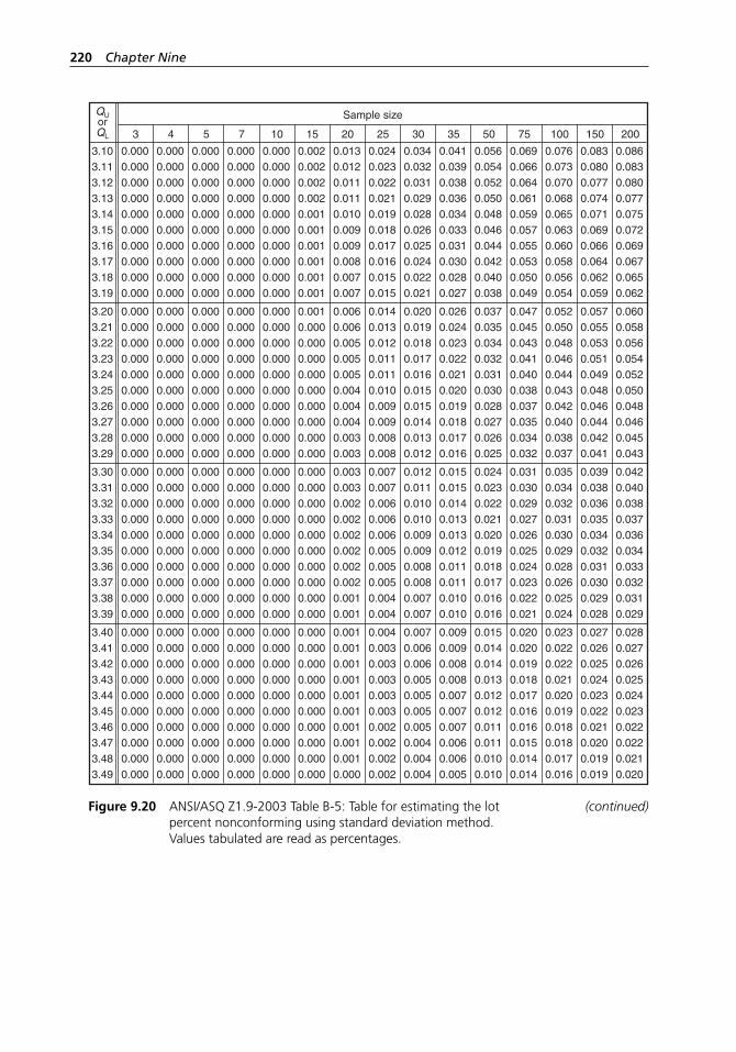
220 Chapter Nine
Sample sizeQUorQL
3.103.113.123.133.143.153.163.173.183.19
0.0000.0000.0000.0000.0000.0000.0000.0000.0000.000
0.0000.0000.0000.0000.0000.0000.0000.0000.0000.000
0.0000.0000.0000.0000.0000.0000.0000.0000.0000.000
0.0000.0000.0000.0000.0000.0000.0000.0000.0000.000
0.0000.0000.0000.0000.0000.0000.0000.0000.0000.000
0.0020.0020.0020.0020.0010.0010.0010.0010.0010.001
0.0130.0120.0110.0110.0100.0090.0090.0080.0070.007
0.0240.0230.0220.0210.0190.0180.0170.0160.0150.015
0.0340.0320.0310.0290.0280.0260.0250.0240.0220.021
0.0410.0390.0380.0360.0340.0330.0310.0300.0280.027
0.0560.0540.0520.0500.0480.0460.0440.0420.0400.038
0.0690.0660.0640.0610.0590.0570.0550.0530.0500.049
0.0760.0730.0700.0680.0650.0630.0600.0580.0560.054
0.0830.0800.0770.0740.0710.0690.0660.0640.0620.059
0.0860.0830.0800.0770.0750.0720.0690.0670.0650.062
3.203.213.223.233.243.253.263.273.283.29
0.0000.0000.0000.0000.0000.0000.0000.0000.0000.000
0.0000.0000.0000.0000.0000.0000.0000.0000.0000.000
0.0000.0000.0000.0000.0000.0000.0000.0000.0000.000
0.0000.0000.0000.0000.0000.0000.0000.0000.0000.000
0.0000.0000.0000.0000.0000.0000.0000.0000.0000.000
0.0010.0000.0000.0000.0000.0000.0000.0000.0000.000
0.0060.0060.0050.0050.0050.0040.0040.0040.0030.003
0.0140.0130.0120.0110.0110.0100.0090.0090.0080.008
0.0200.0190.0180.0170.0160.0150.0150.0140.0130.012
0.0260.0240.0230.0220.0210.0200.0190.0180.0170.016
0.0370.0350.0340.0320.0310.0300.0280.0270.0260.025
0.0470.0450.0430.0410.0400.0380.0370.0350.0340.032
0.0520.0500.0480.0460.0440.0430.0420.0400.0380.037
0.0570.0550.0530.0510.0490.0480.0460.0440.0420.041
0.0600.0580.0560.0540.0520.0500.0480.0460.0450.043
3.303.313.323.333.343.353.363.373.383.39
0.0000.0000.0000.0000.0000.0000.0000.0000.0000.000
0.0000.0000.0000.0000.0000.0000.0000.0000.0000.000
0.0000.0000.0000.0000.0000.0000.0000.0000.0000.000
0.0000.0000.0000.0000.0000.0000.0000.0000.0000.000
0.0000.0000.0000.0000.0000.0000.0000.0000.0000.000
0.0000.0000.0000.0000.0000.0000.0000.0000.0000.000
0.0030.0030.0020.0020.0020.0020.0020.0020.0010.001
0.0070.0070.0060.0060.0060.0050.0050.0050.0040.004
0.0120.0110.0100.0100.0090.0090.0080.0080.0070.007
0.0150.0150.0140.0130.0130.0120.0110.0110.0100.010
0.0240.0230.0220.0210.0200.0190.0180.0170.0160.016
0.0310.0300.0290.0270.0260.0250.0240.0230.0220.021
0.0350.0340.0320.0310.0300.0290.0280.0260.0250.024
0.0390.0380.0360.0350.0340.0320.0310.0300.0290.028
0.0420.0400.0380.0370.0360.0340.0330.0320.0310.029
3.403.413.423.433.443.453.463.473.483.49
0.0000.0000.0000.0000.0000.0000.0000.0000.0000.000
0.0000.0000.0000.0000.0000.0000.0000.0000.0000.000
0.0000.0000.0000.0000.0000.0000.0000.0000.0000.000
0.0000.0000.0000.0000.0000.0000.0000.0000.0000.000
0.0000.0000.0000.0000.0000.0000.0000.0000.0000.000
0.0000.0000.0000.0000.0000.0000.0000.0000.0000.000
0.0010.0010.0010.0010.0010.0010.0010.0010.0010.000
0.0040.0030.0030.0030.0030.0030.0020.0020.0020.002
0.0070.0060.0060.0050.0050.0050.0050.0040.0040.004
0.0090.0090.0080.0080.0070.0070.0070.0060.0060.005
0.0150.0140.0140.0130.0120.0120.0110.0110.0100.010
0.0200.0200.0190.0180.0170.0160.0160.0150.0140.014
0.0230.0220.0220.0210.0200.0190.0180.0180.0170.016
0.0270.0260.0250.0240.0230.0220.0210.0200.0190.019
0.0280.0270.0260.0250.0240.0230.0220.0220.0210.020
3 4 5 7 10 15 20 25 30 35 50 75 100 150 200
Figure 9.20 ANSI/ASQ Z1.9-2003 Table B-5: Table for estimating the lot (continued)percent nonconforming using standard deviation method.
Values tabulated are read as percentages.
H1277 ch09.indd 220H1277 ch09.indd 220 3/8/07 12:38:15 PM3/8/07 12:38:15 PM
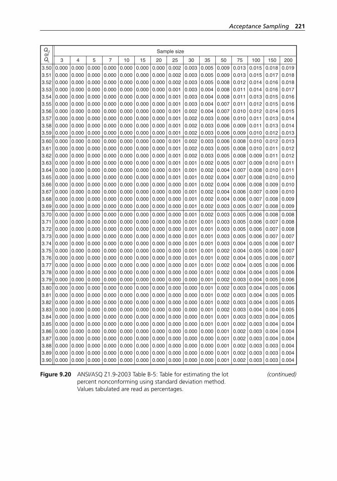
Acceptance Sampling 221
Sample sizeQUorQL
3.503.513.523.533.543.553.563.573.583.59
0.0000.0000.0000.0000.0000.0000.0000.0000.0000.000
0.0000.0000.0000.0000.0000.0000.0000.0000.0000.000
0.0000.0000.0000.0000.0000.0000.0000.0000.0000.000
0.0000.0000.0000.0000.0000.0000.0000.0000.0000.000
0.0000.0000.0000.0000.0000.0000.0000.0000.0000.000
0.0000.0000.0000.0000.0000.0000.0000.0000.0000.000
0.0000.0000.0000.0000.0000.0000.0000.0000.0000.000
0.0020.0020.0020.0010.0010.0010.0010.0010.0010.001
0.0030.0030.0030.0030.0030.0030.0020.0020.0020.002
0.0050.0050.0050.0040.0040.0040.0040.0030.0030.003
0.0090.0090.0080.0080.0080.0070.0070.0060.0060.006
0.0130.0130.0120.0110.0110.0110.0100.0100.0090.009
0.0150.0150.0140.0140.0130.0120.0120.0110.0110.010
0.0180.0170.0160.0160.0150.0150.0140.0130.0130.012
0.0190.0180.0180.0170.0160.0160.0150.0140.0140.013
3.603.613.623.633.643.653.663.673.683.69
0.0000.0000.0000.0000.0000.0000.0000.0000.0000.000
0.0000.0000.0000.0000.0000.0000.0000.0000.0000.000
0.0000.0000.0000.0000.0000.0000.0000.0000.0000.000
0.0000.0000.0000.0000.0000.0000.0000.0000.0000.000
0.0000.0000.0000.0000.0000.0000.0000.0000.0000.000
0.0000.0000.0000.0000.0000.0000.0000.0000.0000.000
0.0000.0000.0000.0000.0000.0000.0000.0000.0000.000
0.0010.0010.0010.0010.0010.0010.0000.0000.0000.000
0.0020.0020.0020.0010.0010.0010.0010.0010.0010.001
0.0030.0030.0030.0020.0020.0020.0020.0020.0020.002
0.0060.0050.0050.0050.0040.0040.0040.0040.0040.003
0.0080.0080.0080.0070.0070.0070.0060.0060.0060.005
0.0100.0100.0090.0090.0080.0080.0080.0070.0070.007
0.0120.0110.0110.0100.0100.0100.0090.0090.0080.008
0.0130.0120.0120.0110.0110.0100.0100.0100.0090.009
3.703.713.723.733.743.753.763.773.783.79
0.0000.0000.0000.0000.0000.0000.0000.0000.0000.000
0.0000.0000.0000.0000.0000.0000.0000.0000.0000.000
0.0000.0000.0000.0000.0000.0000.0000.0000.0000.000
0.0000.0000.0000.0000.0000.0000.0000.0000.0000.000
0.0000.0000.0000.0000.0000.0000.0000.0000.0000.000
0.0000.0000.0000.0000.0000.0000.0000.0000.0000.000
0.0000.0000.0000.0000.0000.0000.0000.0000.0000.000
0.0000.0000.0000.0000.0000.0000.0000.0000.0000.000
0.0010.0010.0010.0010.0010.0010.0010.0010.0000.000
0.0020.0010.0010.0010.0010.0010.0010.0010.0010.001
0.0030.0030.0030.0030.0030.0020.0020.0020.0020.002
0.0050.0050.0050.0050.0040.0040.0040.0040.0040.003
0.0060.0060.0060.0060.0050.0050.0050.0050.0040.004
0.0080.0070.0070.0070.0060.0060.0060.0060.0050.005
0.0080.0080.0080.0070.0070.0070.0070.0060.0060.006
3.803.813.823.833.843.853.863.873.883.893.90
0.0000.0000.0000.0000.0000.0000.0000.0000.0000.0000.000
0.0000.0000.0000.0000.0000.0000.0000.0000.0000.0000.000
0.0000.0000.0000.0000.0000.0000.0000.0000.0000.0000.000
0.0000.0000.0000.0000.0000.0000.0000.0000.0000.0000.000
0.0000.0000.0000.0000.0000.0000.0000.0000.0000.0000.000
0.0000.0000.0000.0000.0000.0000.0000.0000.0000.0000.000
0.0000.0000.0000.0000.0000.0000.0000.0000.0000.0000.000
0.0000.0000.0000.0000.0000.0000.0000.0000.0000.0000.000
0.0000.0000.0000.0000.0000.0000.0000.0000.0000.0000.000
0.0010.0010.0010.0010.0010.0010.0000.0000.0000.0000.000
0.0020.0020.0020.0020.0010.0010.0010.0010.0010.0010.001
0.0030.0030.0030.0030.0030.0020.0020.0020.0020.0020.002
0.0040.0040.0040.0040.0030.0030.0030.0030.0030.0030.003
0.0050.0050.0050.0040.0040.0040.0040.0040.0030.0030.003
0.0060.0050.0050.0050.0050.0040.0040.0040.0040.0040.004
3 4 5 7 10 15 20 25 30 35 50 75 100 150 200
Figure 9.20 ANSI/ASQ Z1.9-2003 Table B-5: Table for estimating the lot (continued)percent nonconforming using standard deviation method.
Values tabulated are read as percentages.
H1277 ch09.indd 221H1277 ch09.indd 221 3/8/07 12:38:15 PM3/8/07 12:38:15 PM
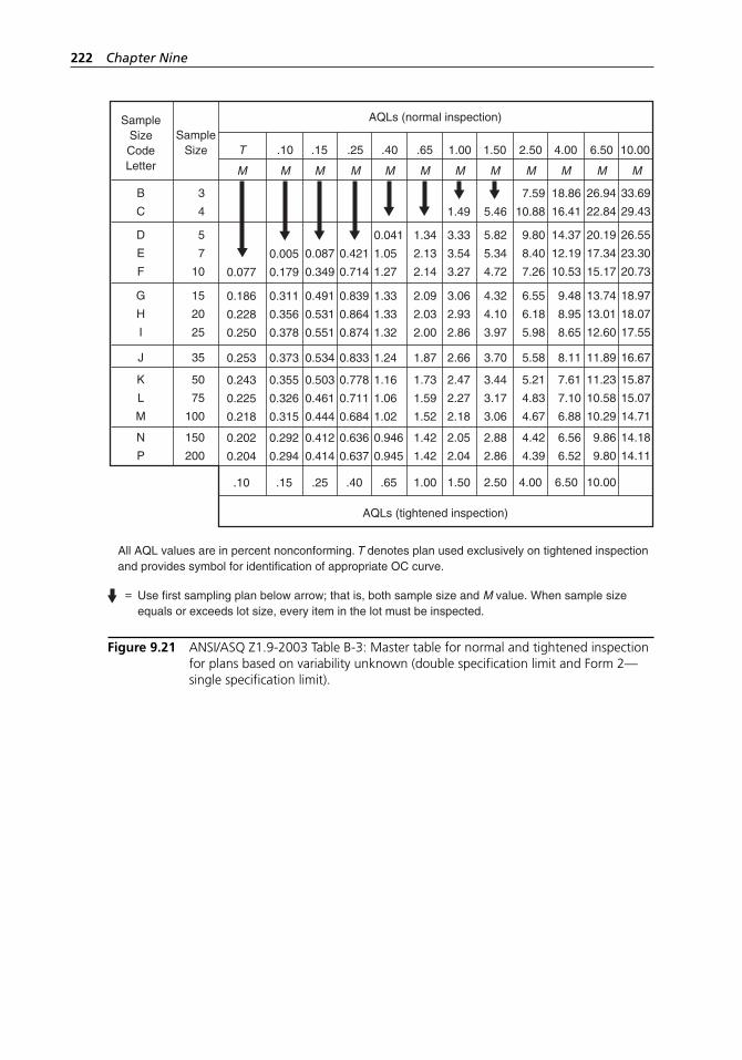
222 Chapter Nine
SampleSizeCodeLetter
SampleSize
AQLs (normal inspection)
AQLs (tightened inspection)
T
M
.10
M
.15
M
.25
M
.40
M
.65
M
1.00
M
1.50
M
2.50
M
4.00
M
6.50
M
10.00
M
B
C
D
E
F
G
H
I
K
L
M
N
P
J
3
4
5
7
10
15
20
25
50
75
100
150
200
35
33.69
29.43
26.55
23.30
20.73
18.97
18.07
17.55
15.87
15.07
14.71
14.18
14.11
16.67
26.94
22.84
20.19
17.34
15.17
13.74
13.01
12.60
11.23
10.58
10.29
9.86
9.80
10.00
11.89
18.86
16.41
14.37
12.19
10.53
9.48
8.95
8.65
7.61
7.10
6.88
6.56
6.52
6.50
8.11
7.59
10.88
9.80
8.40
7.26
6.55
6.18
5.98
5.21
4.83
4.67
4.42
4.39
4.00
5.58
5.46
5.82
5.34
4.72
4.32
4.10
3.97
3.44
3.17
3.06
2.88
2.86
2.50
3.70
1.49
3.33
3.54
3.27
3.06
2.93
2.86
2.47
2.27
2.18
2.05
2.04
1.50
2.66
1.34
2.13
2.14
2.09
2.03
2.00
1.73
1.59
1.52
1.42
1.42
1.00
1.87
0.041
1.05
1.27
1.33
1.33
1.32
1.16
1.06
1.02
0.946
0.945
.65
1.24
0.421
0.714
0.839
0.864
0.874
0.778
0.711
0.684
0.636
0.637
.40
0.833
0.087
0.349
0.491
0.531
0.551
0.503
0.461
0.444
0.412
0.414
.25
0.534
0.311
0.356
0.378
0.355
0.326
0.315
0.292
0.294
.15
0.373
0.186
0.228
0.250
0.005
0.1790.077
0.243
0.225
0.218
0.202
0.204
.10
0.253
All AQL values are in percent nonconforming. T denotes plan used exclusively on tightened inspection and provides symbol for identification of appropriate OC curve.
Use first sampling plan below arrow; that is, both sample size and M value. When sample size equals or exceeds lot size, every item in the lot must be inspected.
=
Figure 9.21 ANSI/ASQ Z1.9-2003 Table B-3: Master table for normal and tightened inspection for plans based on variability unknown (double specification limit and Form 2—single specification limit).
H1277 ch09.indd 222H1277 ch09.indd 222 3/8/07 12:38:15 PM3/8/07 12:38:15 PM

Acceptance Sampling 223
Notes
1. W. E. Deming, Out of the Crisis (Cambridge, MA: MIT Center for Advanced Engineer-ing, 1986).
2. J. M. Juran and F. N. Gryna Jr., Quality Planning and Analysis (New York: McGraw- Hill, 1980).
3. ASQ Statistics Division, Glossary and Tables for Statistical Quality Control, 4th ed. (Milwaukee, WI: ASQ Quality Press, 2004).
4. Ibid. 5. ANSI/ASQ Z1.4-2003, Sampling Procedures and Tables for Inspection by Attributes
(Milwaukee, WI: ASQ Quality Press, 2003). 6. Deming, Crisis. 7. A. Wald, Sequential Analysis (New York: Dover, 1973). 8. W. Burr, Statistical Quality Control Methods (New York: Marcel Dekker, 1976).
H1277 ch09.indd 223H1277 ch09.indd 223 3/8/07 12:38:15 PM3/8/07 12:38:15 PM

H1277 ch09.indd 224H1277 ch09.indd 224 3/8/07 12:38:15 PM3/8/07 12:38:15 PM

225
In the past two decades, the use of technology to analyze complicated data has increased substantially, which not only has made the analysis much easier, but also has reduced the time required to complete the analy-
sis. To facilitate statistical analysis, many companies use personal computer (PC)–based statistical application software. Several software packages are available, including BMDP, JMP, MINITAB, SAS, SPSS, and SYSTAT, to name a few. A great deal of effort has been expended in the development of these software packages to create graphical user interfaces that allow soft-ware users to complete statistical analysis activities without having to know a computer programming or scripting language. We believe that publishing a book about applied statistics without acknowledging and addressing the importance and usefulness of statistical software is not in the best interests of the reader. Accordingly, in this and the next chapter, we will briefly discuss two very popular statistical packages: MINITAB and JMP. It is our explicit intent not to endorse either software package, as each has different strengths and features/capabilities.
10.1 Using MINITAB—Version 14
MINITAB has the option of using commands from the menu bar, typing in Session commands, or using both. As shown in Figure 10.1 in the Windows environment, it has the look and feel of most other Windows applications, where the menu options help you to easily navigate through the software.
Once you are in MINITAB, you will see the heading MINITAB - Unti-tled and three windows:
1. The Data window (Worksheet) is used to enter data in columns labeled C1, C2, C3, . . . , C4000.
2. The Session window displays the output and also allows you to enter commands when using the command language.
10
Computer Resources to Support SQC: MINITAB
H1277 ch10.indd 225H1277 ch10.indd 225 3/8/07 6:07:44 PM3/8/07 6:07:44 PM
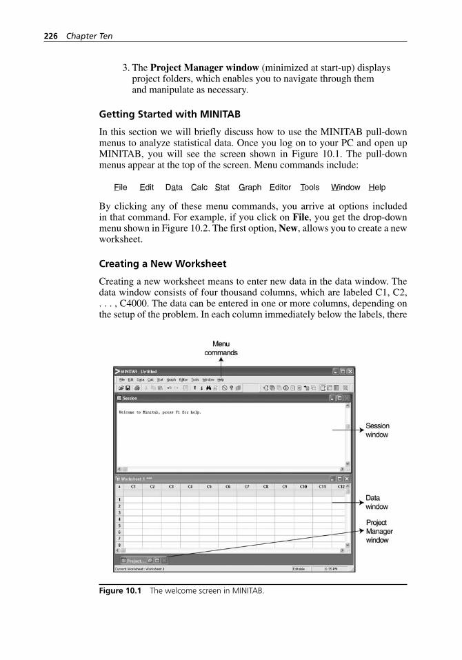
226 Chapter Ten
3. The Project Manager window (minimized at start- up) displays project folders, which enables you to navigate through them and manipulate as necessary.
Getting Started with MINITAB
In this section we will briefly discuss how to use the MINITAB pull- down menus to analyze statistical data. Once you log on to your PC and open up MINITAB, you will see the screen shown in Figure 10.1. The pull- down menus appear at the top of the screen. Menu commands include:
File Edit Data Calc Stat Graph Editor Tools Window Help
By clicking any of these menu commands, you arrive at options included in that command. For example, if you click on File, you get the drop- down menu shown in Figure 10.2. The first option, New, allows you to create a new worksheet.
Creating a New Worksheet
Creating a new worksheet means to enter new data in the data window. The data window consists of four thousand columns, which are labeled C1, C2, . . . , C4000. The data can be entered in one or more columns, depending on the setup of the problem. In each column immediately below the labels, there
Figure 10.1 The welcome screen in MINITAB.
H1277 ch10.indd 226H1277 ch10.indd 226 3/8/07 6:07:44 PM3/8/07 6:07:44 PM
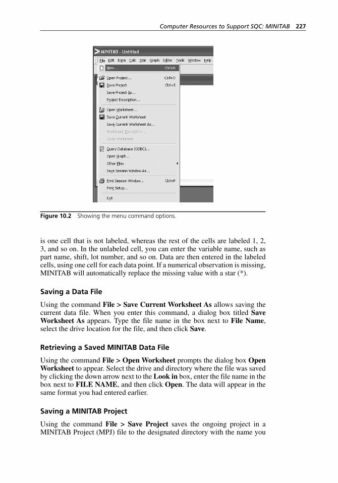
Computer Resources to Support SQC: MINITAB 227
is one cell that is not labeled, whereas the rest of the cells are labeled 1, 2, 3, and so on. In the unlabeled cell, you can enter the variable name, such as part name, shift, lot number, and so on. Data are then entered in the labeled cells, using one cell for each data point. If a numerical observation is missing, MINITAB will automatically replace the missing value with a star (*).
Saving a Data File
Using the command File > Save Current Worksheet As allows saving the current data file. When you enter this command, a dialog box titled Save Worksheet As appears. Type the file name in the box next to File Name, select the drive location for the file, and then click Save.
Retrieving a Saved MINITAB Data File
Using the command File > Open Worksheet prompts the dialog box Open Worksheet to appear. Select the drive and directory where the file was saved by clicking the down arrow next to the Look in box, enter the file name in the box next to FILE NAME, and then click Open. The data will appear in the same format you had entered earlier.
Saving a MINITAB Project
Using the command File > Save Project saves the ongoing project in a MINITAB Project (MPJ) file to the designated directory with the name you
Figure 10.2 Showing the menu command options.
H1277 ch10.indd 227H1277 ch10.indd 227 3/8/07 6:07:44 PM3/8/07 6:07:44 PM
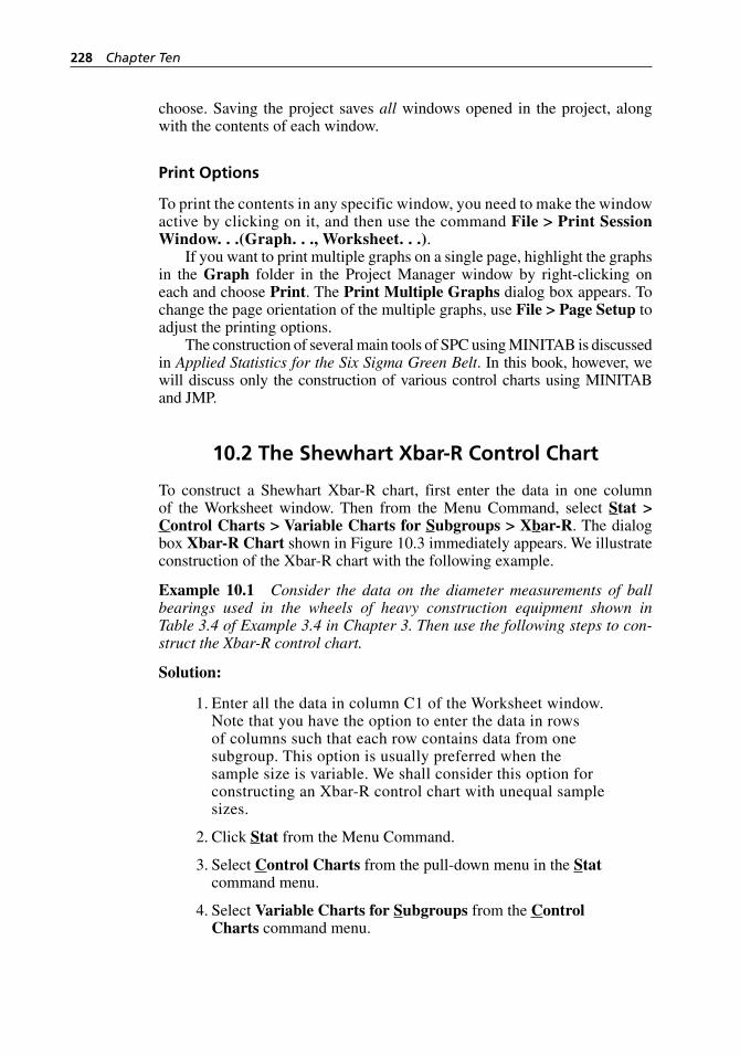
228 Chapter Ten
choose. Saving the project saves all windows opened in the project, along with the contents of each window.
Print Options
To print the contents in any specific window, you need to make the window active by clicking on it, and then use the command File > Print SessionWindow. . .(Graph. . ., Worksheet. . .).
If you want to print multiple graphs on a single page, highlight the graphs in the Graph folder in the Project Manager window by right- clicking on each and choose Print. The Print Multiple Graphs dialog box appears. To change the page orientation of the multiple graphs, use File > Page Setup to adjust the printing options.
The construction of several main tools of SPC using MINITAB is discussed in Applied Statistics for the Six Sigma Green Belt. In this book, however, we will discuss only the construction of various control charts using MINITAB and JMP.
10.2 The Shewhart Xbar- R Control Chart
To construct a Shewhart Xbar- R chart, first enter the data in one column of the Worksheet window. Then from the Menu Command, select Stat > Control Charts > Variable Charts for Subgroups > Xbar-R. The dialog box Xbar-R Chart shown in Figure 10.3 immediately appears. We illustrate construction of the Xbar- R chart with the following example.
Example 10.1 Consider the data on the diameter measurements of ball bearings used in the wheels of heavy construction equipment shown in Table 3.4 of Example 3.4 in Chapter 3. Then use the following steps to con-struct the Xbar- R control chart.
Solution:
1. Enter all the data in column C1 of the Worksheet window. Note that you have the option to enter the data in rows of columns such that each row contains data from one subgroup. This option is usually preferred when the sample size is variable. We shall consider this option for constructing an Xbar- R control chart with unequal sample sizes.
2. Click Stat from the Menu Command.
3. Select Control Charts from the pull- down menu in the Stat command menu.
4. Select Variable Charts for Subgroups from the Control Charts command menu.
H1277 ch10.indd 228H1277 ch10.indd 228 3/8/07 6:07:44 PM3/8/07 6:07:44 PM
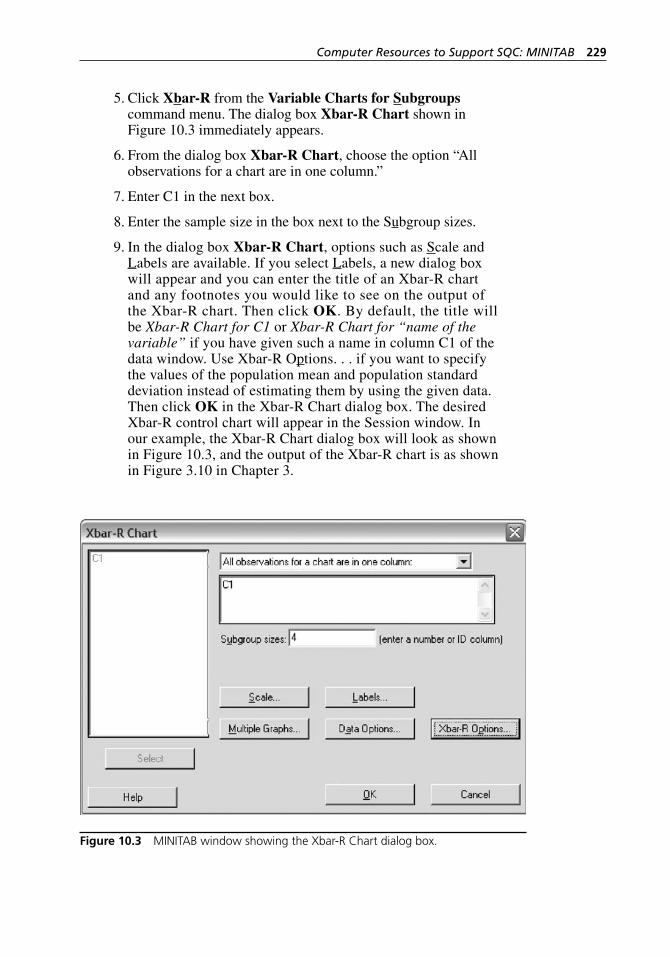
Computer Resources to Support SQC: MINITAB 229
5. Click Xbar-R from the Variable Charts for Subgroups command menu. The dialog box Xbar-R Chart shown in Figure 10.3 immediately appears.
6. From the dialog box Xbar-R Chart, choose the option “All observations for a chart are in one column.”
7. Enter C1 in the next box.
8. Enter the sample size in the box next to the Subgroup sizes.
9. In the dialog box Xbar-R Chart, options such as Scale and Labels are available. If you select Labels, a new dialog box will appear and you can enter the title of an Xbar- R chart and any footnotes you would like to see on the output of the Xbar- R chart. Then click OK. By default, the title will be Xbar-R Chart for C1 or Xbar-R Chart for “name of the variable” if you have given such a name in column C1 of the data window. Use Xbar- R Options. . . if you want to specify the values of the population mean and population standard deviation instead of estimating them by using the given data. Then click OK in the Xbar- R Chart dialog box. The desired Xbar- R control chart will appear in the Session window. In our example, the Xbar- R Chart dialog box will look as shown in Figure 10.3, and the output of the Xbar- R chart is as shown in Figure 3.10 in Chapter 3.
Figure 10.3 MINITAB window showing the Xbar-R Chart dialog box.
H1277 ch10.indd 229H1277 ch10.indd 229 3/8/07 6:07:44 PM3/8/07 6:07:44 PM
230 Chapter Ten
10.3 The Shewhart Xbar- R Control Chart When Process Mean and Process Standard Deviation Are Known
To construct a Shewhart Xbar- R control chart when process mean µ and pro-cess standard deviation σ are known, follow steps 1 through 8 of the solution shown in Example 10.1. Then click Xbar- R Options. . . . A new dialog box, shown in Figure 10.4, will appear. In the boxes next to Mean and Standard deviation, enter the specified values and then click OK. Then click OK again in the Xbar- R Chart dialog box. The desired Xbar- R control chart will appear in the Session window.
10.4 The Shewhart Control Chart for Individual Observations
To construct a Shewhart control chart for individual observations, first enter the data in one column, say C1, of the Worksheet window. Then from the Menu Command, select Stat > Control Charts > Variable Charts for Indi-viduals > I-MR. The dialog box Individuals-Moving Range Chart, shown in Figure 10.5, appears. We illustrate the construction of a Shewhart control chart for individual observations with the following example.
Example 10.2 Consider the data on the diameter measurements of ball bearings used in the wheels of heavy construction equipment shown in Table 3.5 of Example 3.6 in Chapter 3. Then use the following steps to con-struct the Shewhart control chart for individual observations.
Figure 10.4 MINITAB window showing the Xbar-R Chart - Options dialog box.
H1277 ch10.indd 230H1277 ch10.indd 230 3/8/07 6:07:45 PM3/8/07 6:07:45 PM
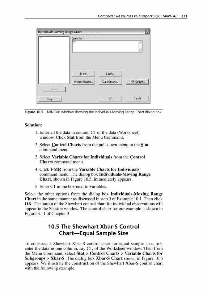
Computer Resources to Support SQC: MINITAB 231
Solution:
1. Enter all the data in column C1 of the data (Worksheet) window. Click Stat from the Menu Command.
2. Select Control Charts from the pull- down menu in the Stat command menu.
3. Select Variable Charts for Individuals from the Control Charts command menu.
4. Click I-MR from the Variable Charts for Individuals command menu. The dialog box Individuals-Moving Range Chart, shown in Figure 10.5, immediately appears.
5. Enter C1 in the box next to Variables.
Select the other options from the dialog box Individuals-Moving Range Chart in the same manner as discussed in step 9 of Example 10.1. Then click OK. The output of the Shewhart control chart for individual observations will appear in the Session window. The control chart for our example is shown in Figure 3.11 of Chapter 3.
10.5 The Shewhart Xbar- S Control Chart—Equal Sample Size
To construct a Shewhart Xbar- S control chart for equal sample size, first enter the data in one column, say C1, of the Worksheet window. Then from the Menu Command, select Stat > Control Charts > Variable Charts for Subgroups > Xbar-S. The dialog box Xbar-S Chart shown in Figure 10.6 appears. We illustrate the construction of the Shewhart Xbar- S control chart with the following example.
Figure 10.5 MINITAB window showing the Individuals- Moving Range Chart dialog box.
H1277 ch10.indd 231H1277 ch10.indd 231 3/8/07 6:07:45 PM3/8/07 6:07:45 PM
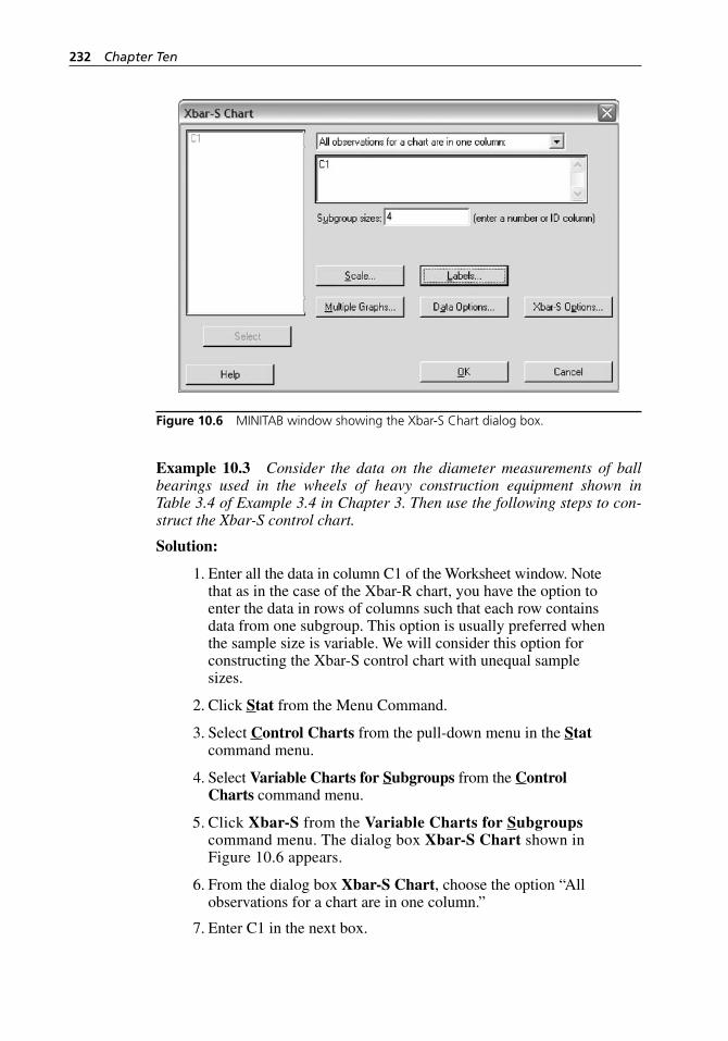
232 Chapter Ten
Example 10.3 Consider the data on the diameter measurements of ball bearings used in the wheels of heavy construction equipment shown in Table 3.4 of Example 3.4 in Chapter 3. Then use the following steps to con-struct the Xbar- S control chart.
Solution:
1. Enter all the data in column C1 of the Worksheet window. Note that as in the case of the Xbar- R chart, you have the option to enter the data in rows of columns such that each row contains data from one subgroup. This option is usually preferred when the sample size is variable. We will consider this option for constructing the Xbar- S control chart with unequal sample sizes.
2. Click Stat from the Menu Command.
3. Select Control Charts from the pull- down menu in the Stat command menu.
4. Select Variable Charts for Subgroups from the Control Charts command menu.
5. Click Xbar-S from the Variable Charts for Subgroups command menu. The dialog box Xbar-S Chart shown in Figure 10.6 appears.
6. From the dialog box Xbar-S Chart, choose the option “All observations for a chart are in one column.”
7. Enter C1 in the next box.
Figure 10.6 MINITAB window showing the Xbar-S Chart dialog box.
H1277 ch10.indd 232H1277 ch10.indd 232 3/8/07 6:07:45 PM3/8/07 6:07:45 PM
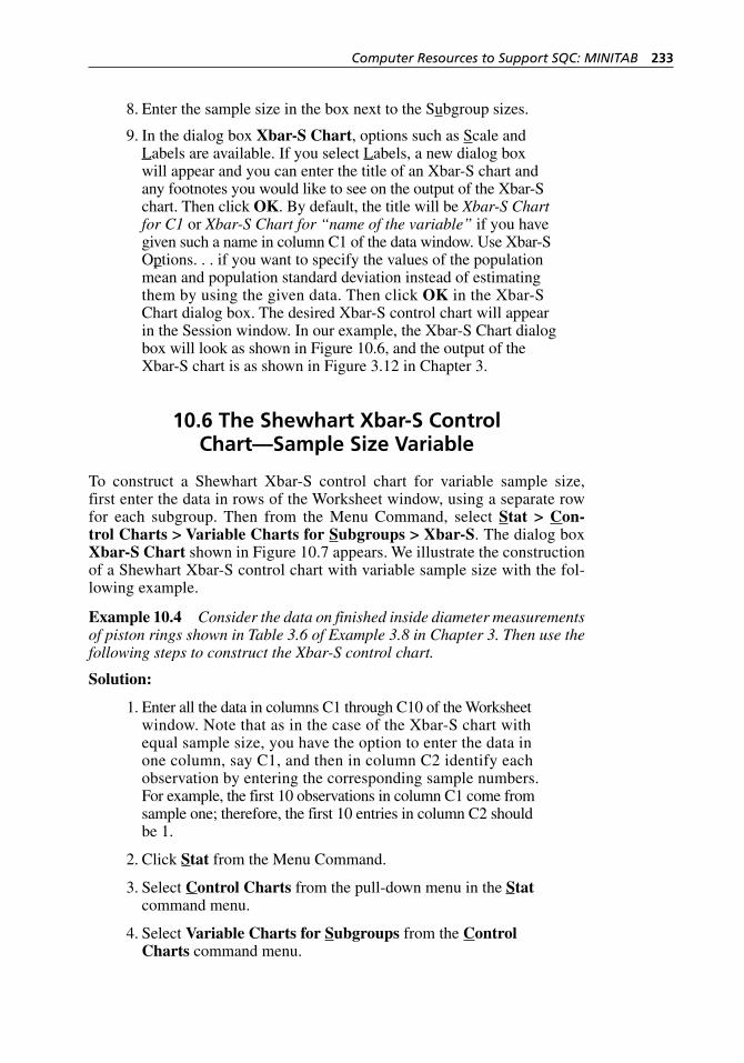
Computer Resources to Support SQC: MINITAB 233
8. Enter the sample size in the box next to the Subgroup sizes.
9. In the dialog box Xbar-S Chart, options such as Scale and Labels are available. If you select Labels, a new dialog box will appear and you can enter the title of an Xbar- S chart and any footnotes you would like to see on the output of the Xbar- S chart. Then click OK. By default, the title will be Xbar-S Chart for C1 or Xbar-S Chart for “name of the variable” if you have given such a name in column C1 of the data window. Use Xbar- S Options. . . if you want to specify the values of the population mean and population standard deviation instead of estimating them by using the given data. Then click OK in the Xbar- S Chart dialog box. The desired Xbar- S control chart will appear in the Session window. In our example, the Xbar- S Chart dialog box will look as shown in Figure 10.6, and the output of the Xbar- S chart is as shown in Figure 3.12 in Chapter 3.
10.6 The Shewhart Xbar- S Control Chart—Sample Size Variable
To construct a Shewhart Xbar- S control chart for variable sample size, first enter the data in rows of the Worksheet window, using a separate row for each subgroup. Then from the Menu Command, select Stat > Con-trol Charts > Variable Charts for Subgroups > Xbar-S. The dialog box Xbar-S Chart shown in Figure 10.7 appears. We illustrate the construction of a Shewhart Xbar- S control chart with variable sample size with the fol-lowing example.
Example 10.4 Consider the data on finished inside diameter measurements of piston rings shown in Table 3.6 of Example 3.8 in Chapter 3. Then use the following steps to construct the Xbar- S control chart.
Solution:
1. Enter all the data in columns C1 through C10 of the Worksheet window. Note that as in the case of the Xbar- S chart with equal sample size, you have the option to enter the data in one column, say C1, and then in column C2 identify each observation by entering the corresponding sample numbers. For example, the first 10 observations in column C1 come from sample one; therefore, the first 10 entries in column C2 should be 1.
2. Click Stat from the Menu Command.
3. Select Control Charts from the pull- down menu in the Stat command menu.
4. Select Variable Charts for Subgroups from the Control Charts command menu.
H1277 ch10.indd 233H1277 ch10.indd 233 3/8/07 6:07:45 PM3/8/07 6:07:45 PM
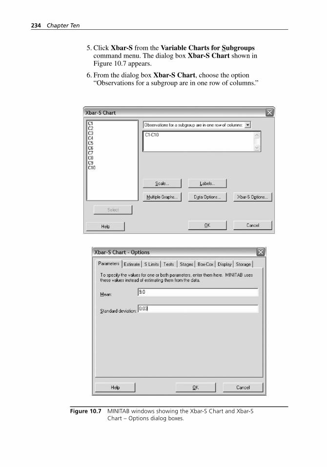
234 Chapter Ten
5. Click Xbar-S from the Variable Charts for Subgroups command menu. The dialog box Xbar-S Chart shown in Figure 10.7 appears.
6. From the dialog box Xbar-S Chart, choose the option “Observations for a subgroup are in one row of columns.”
Figure 10.7 MINITAB windows showing the Xbar- S Chart and Xbar- S Chart – Options dialog boxes.
H1277 ch10.indd 234H1277 ch10.indd 234 3/8/07 6:07:45 PM3/8/07 6:07:45 PM
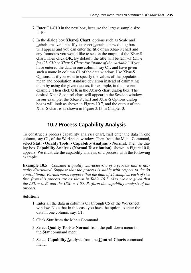
Computer Resources to Support SQC: MINITAB 235
7. Enter C1-C10 in the next box, because the largest sample size is 10.
8. In the dialog box Xbar-S Chart, options such as Scale and Labels are available. If you select Labels, a new dialog box will appear and you can enter the title of an Xbar- S chart and any footnotes you would like to see on the output of the Xbar- S chart. Then click OK. By default, the title will be Xbar-S Chart for C1-C10 or Xbar-S Chart for “name of the variable” if you have entered the data in one column, say C1, and have given such a name in column C1 of the data window. Use Xbar- S Options. . . if you want to specify the values of the population mean and population standard deviation instead of estimating them by using the given data as, for example, in the present example. Then click OK in the Xbar- S chart dialog box. The desired Xbar- S control chart will appear in the Session window. In our example, the Xbar- S chart and Xbar- S Options dialog boxes will look as shown in Figure 10.7, and the output of the Xbar- S chart is as shown in Figure 3.13 in Chapter 3.
10.7 Process Capability Analysis
To construct a process capability analysis chart, first enter the data in one column, say C1, of the Worksheet window. Then from the Menu Command, select Stat > Quality Tools > Capability Analysis > Normal. Then the dia-log box Capability Analysis (Normal Distribution), shown in Figure 10.8, appears. We illustrate the capability analysis of a process with the following example.
Example 10.5 Consider a quality characteristic of a process that is nor-mally distributed. Suppose that the process is stable with respect to the 3σ control limits. Furthermore, suppose that the data of 25 samples, each of size five, from this process are as shown in Table 10.1. Also, we are given that the LSL = 0.95 and the USL = 1.05. Perform the capability analysis of the process.
Solution:
1. Enter all the data in columns C1 through C5 of the Worksheet window. Note that in this case you have the option to enter the data in one column, say, C1.
2. Click Stat from the Menu Command.
3. Select Quality Tools > Normal from the pull- down menu in the Stat command menu.
4. Select Capability Analysis from the Control Charts command menu.
H1277 ch10.indd 235H1277 ch10.indd 235 3/8/07 6:07:46 PM3/8/07 6:07:46 PM
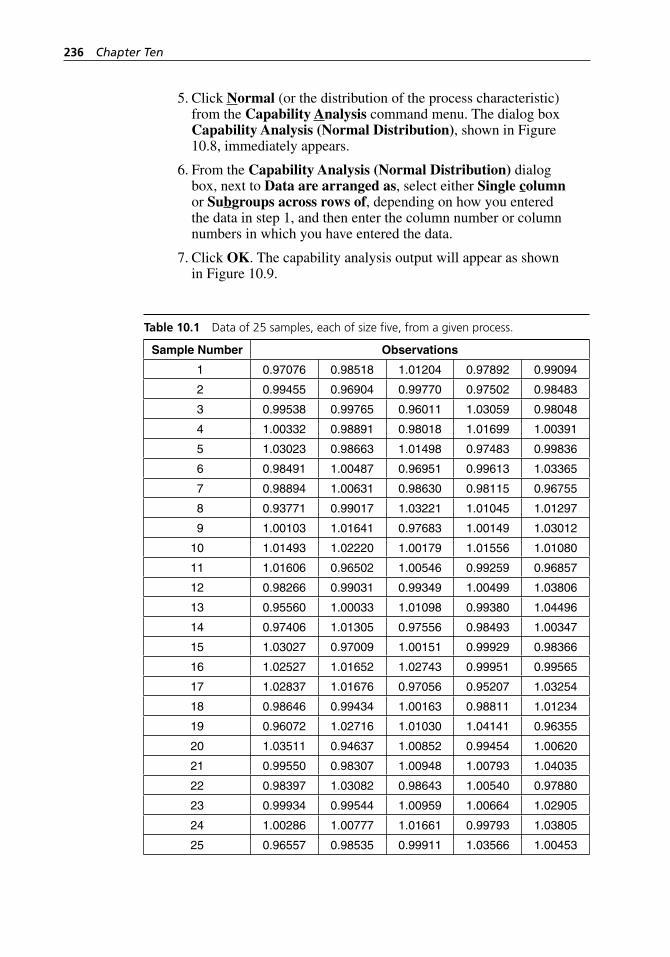
236 Chapter Ten
5. Click Normal (or the distribution of the process characteristic) from the Capability Analysis command menu. The dialog box Capability Analysis (Normal Distribution), shown in Figure 10.8, immediately appears.
6. From the Capability Analysis (Normal Distribution) dialog box, next to Data are arranged as, select either Single column or Subgroups across rows of, depending on how you entered the data in step 1, and then enter the column number or column numbers in which you have entered the data.
7. Click OK. The capability analysis output will appear as shown in Figure 10.9.
Table 10.1 Data of 25 samples, each of size five, from a given process.
Sample Number Observations
1 0.97076 0.98518 1.01204 0.97892 0.99094
2 0.99455 0.96904 0.99770 0.97502 0.98483
3 0.99538 0.99765 0.96011 1.03059 0.98048
4 1.00332 0.98891 0.98018 1.01699 1.00391
5 1.03023 0.98663 1.01498 0.97483 0.99836
6 0.98491 1.00487 0.96951 0.99613 1.03365
7 0.98894 1.00631 0.98630 0.98115 0.96755
8 0.93771 0.99017 1.03221 1.01045 1.01297
9 1.00103 1.01641 0.97683 1.00149 1.03012
10 1.01493 1.02220 1.00179 1.01556 1.01080
11 1.01606 0.96502 1.00546 0.99259 0.96857
12 0.98266 0.99031 0.99349 1.00499 1.03806
13 0.95560 1.00033 1.01098 0.99380 1.04496
14 0.97406 1.01305 0.97556 0.98493 1.00347
15 1.03027 0.97009 1.00151 0.99929 0.98366
16 1.02527 1.01652 1.02743 0.99951 0.99565
17 1.02837 1.01676 0.97056 0.95207 1.03254
18 0.98646 0.99434 1.00163 0.98811 1.01234
19 0.96072 1.02716 1.01030 1.04141 0.96355
20 1.03511 0.94637 1.00852 0.99454 1.00620
21 0.99550 0.98307 1.00948 1.00793 1.04035
22 0.98397 1.03082 0.98643 1.00540 0.97880
23 0.99934 0.99544 1.00959 1.00664 1.02905
24 1.00286 1.00777 1.01661 0.99793 1.03805
25 0.96557 0.98535 0.99911 1.03566 1.00453
H1277 ch10.indd 236H1277 ch10.indd 236 3/8/07 6:07:46 PM3/8/07 6:07:46 PM
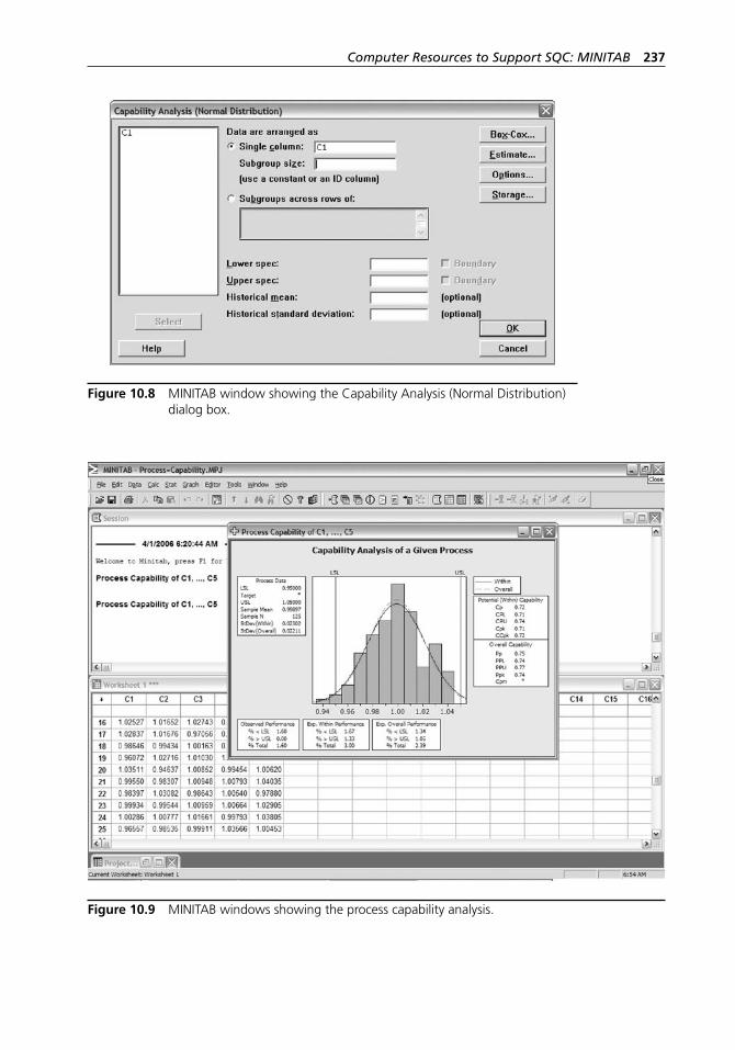
Computer Resources to Support SQC: MINITAB 237
Figure 10.8 MINITAB window showing the Capability Analysis (Normal Distribution) dialog box.
Figure 10.9 MINITAB windows showing the process capability analysis.
H1277 ch10.indd 237H1277 ch10.indd 237 3/8/07 6:07:46 PM3/8/07 6:07:46 PM
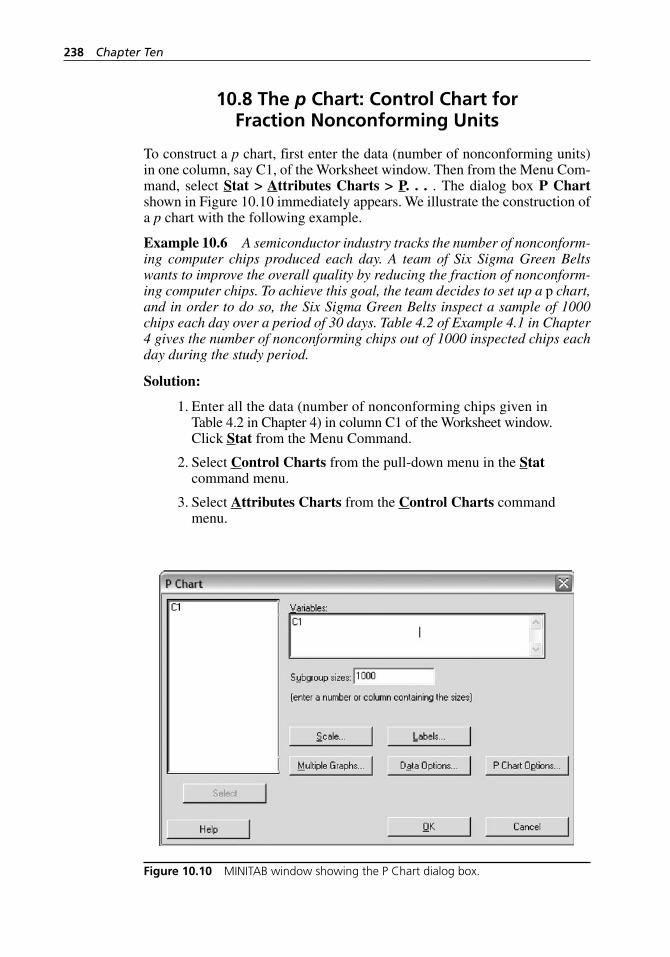
238 Chapter Ten
10.8 The p Chart: Control Chart for Fraction Nonconforming Units
To construct a p chart, first enter the data (number of nonconforming units) in one column, say C1, of the Worksheet window. Then from the Menu Com-mand, select Stat > Attributes Charts > P. . . . The dialog box P Chart shown in Figure 10.10 immediately appears. We illustrate the construction of a p chart with the following example.
Example 10.6 A semiconductor industry tracks the number of nonconform-ing computer chips produced each day. A team of Six Sigma Green Belts wants to improve the overall quality by reducing the fraction of nonconform-ing computer chips. To achieve this goal, the team decides to set up a p chart, and in order to do so, the Six Sigma Green Belts inspect a sample of 1000 chips each day over a period of 30 days. Table 4.2 of Example 4.1 in Chapter 4 gives the number of nonconforming chips out of 1000 inspected chips each day during the study period.
Solution:
1. Enter all the data (number of nonconforming chips given in Table 4.2 in Chapter 4) in column C1 of the Worksheet window. Click Stat from the Menu Command.
2. Select Control Charts from the pull- down menu in the Stat command menu.
3. Select Attributes Charts from the Control Charts command menu.
Figure 10.10 MINITAB window showing the P Chart dialog box.
H1277 ch10.indd 238H1277 ch10.indd 238 3/8/07 6:07:46 PM3/8/07 6:07:46 PM
Computer Resources to Support SQC: MINITAB 239
4. Click P. . . from the Attributes Charts command menu. The dialog box P Chart shown in Figure 10.10 appears.
5. Enter C1 in the box next to Variables.
6. Enter the sample size in the box next to the Subgroup sizes.
7. In the dialog box P Chart, options such as Scale and Labels are available. If you select Labels, a new dialog box will appear and you can enter the title of a p chart and any footnotes you would like to see on the output of the p chart. Then click OK. By default, the title will be P Chart for C1 or P Chart for “name of the variable” if you have given such a name in column C1 of the data window. Use P Chart Options. . . if you want to specify the values of fraction of nonconforming in the population instead of estimating them using the given data. Then click OK in the P Chart dialog box. The desired p control chart will appear in the Session window. Thus, in our example, the output of the p chart is shown in Figure 4.1 in Chapter 4.
10.9 The p Chart: Control Chart for Fraction Nonconforming Units with Variable Sample Size
Constructing a p chart with variable sample size is the same as construct-ing a p chart with fixed sample size, except in this case we enter the data on number of nonconforming units in column C1 and the corresponding sample sizes in column C2; and in step 6, instead of entering the sample size in the box next to the Subgroup sizes, we enter C2.
10.10 The np Chart: Control Chart for Nonconforming Units
In an np chart we plot the number of nonconforming units in an inspected sample. The np chart is very similar to the p chart, except that in the p chart we plot the fraction nonconforming units in each inspected sample. More-over, in a p chart the sample sizes could be equal or unequal, whereas in an np chart, the sample sizes are equal. Otherwise, a p chart and an np chart can be implemented under the same circumstances. We summarize here some specific points that are important for an np chart:
The inspection sample sizes should be equal
The sample size should be large enough to include some noncon-forming units
Record the sample size and number of nonconforming units (np) in each sample and plot the number of nonconforming units on the control chart.
To construct an np control chart, follow all the steps for a p control chart in section 10.8.
•
•
H1277 ch10.indd 239H1277 ch10.indd 239 3/8/07 6:07:46 PM3/8/07 6:07:46 PM

240 Chapter Ten
10.11 The c Chart
In many situations, we are interested in studying the number of nonconformi-ties in a sample, which is also called the inspection unit, rather than studying the fraction nonconforming or total number of nonconforming in the sample. To construct the c chart, first enter the data (number of nonconformities) in one column, say C1, of the Worksheet window. Then from the Menu Com-mand, select Stat > Attributes Charts > C. . . The dialog box C Chart, shown in Figure 10.11, immediately appears. We illustrate the construction of a c chart with the following example.
Example 10.7 A paper mill has detected that almost 90 percent of rejected paper rolls are due to nonconformities of two types: holes and wrinkles in the paper. The Six Sigma Green Belt team in the mill decides to set up control charts to reduce or eliminate the number of these nonconformities. To set up the control charts, the team collects data by taking random samples of five rolls each day for 30 days and counting the number of nonconformities (holes and wrinkles) in each sample. The data are shown in Table 4.4 of Example 4.4 in Chapter 4. Set up a c control chart using these data.
Solution:
1. Enter all the data (number of nonconformities given in Table 4.4 in Chapter 4) in column C1 of the Worksheet window. Click Stat from the Menu Command.
2. Select Control Charts from the pull- down menu in the Stat command menu.
3. Select Attributes Charts from the Control Charts command menu.
4. Click C. . . from the Attributes Charts command menu. The dialog box C Chart, shown in Figure 10.11, appears.
5. Enter C1 in the box next to Variables.
6. In the dialog box C Chart, options such as Scale and Labels are available. If you select Labels, a new dialog box will appear and you can enter the title of a c chart and any footnotes you would like to see on the output of the c chart. Then click OK. By default, the title will be C Chart for C1 or C Chart for “name of the variable” if you have given such a name, say “nonconformities,” in column C1 of the data window. Use C Chart Options. . . if you want to specify the mean value of nonconformities in the population instead of estimating it using the given data. Then click OK in the C chart dialog box. The desired c control chart will appear in the Session window. Thus, in our example, the output of the c chart is shown in Figure 4.4 in Chapter 4.
H1277 ch10.indd 240H1277 ch10.indd 240 3/8/07 6:07:46 PM3/8/07 6:07:46 PM
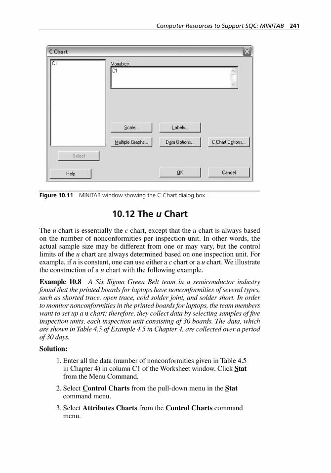
Computer Resources to Support SQC: MINITAB 241
10.12 The u Chart
The u chart is essentially the c chart, except that the u chart is always based on the number of nonconformities per inspection unit. In other words, the actual sample size may be different from one or may vary, but the control limits of the u chart are always determined based on one inspection unit. For example, if n is constant, one can use either a c chart or a u chart. We illustrate the construction of a u chart with the following example.
Example 10.8 A Six Sigma Green Belt team in a semiconductor industry found that the printed boards for laptops have nonconformities of several types, such as shorted trace, open trace, cold solder joint, and solder short. In order to monitor nonconformities in the printed boards for laptops, the team members want to set up a u chart; therefore, they collect data by selecting samples of five inspection units, each inspection unit consisting of 30 boards. The data, which are shown in Table 4.5 of Example 4.5 in Chapter 4, are collected over a period of 30 days.
Solution:
1. Enter all the data (number of nonconformities given in Table 4.5 in Chapter 4) in column C1 of the Worksheet window. Click Stat from the Menu Command.
2. Select Control Charts from the pull- down menu in the Stat command menu.
3. Select Attributes Charts from the Control Charts command menu.
Figure 10.11 MINITAB window showing the C Chart dialog box.
H1277 ch10.indd 241H1277 ch10.indd 241 3/8/07 6:07:47 PM3/8/07 6:07:47 PM
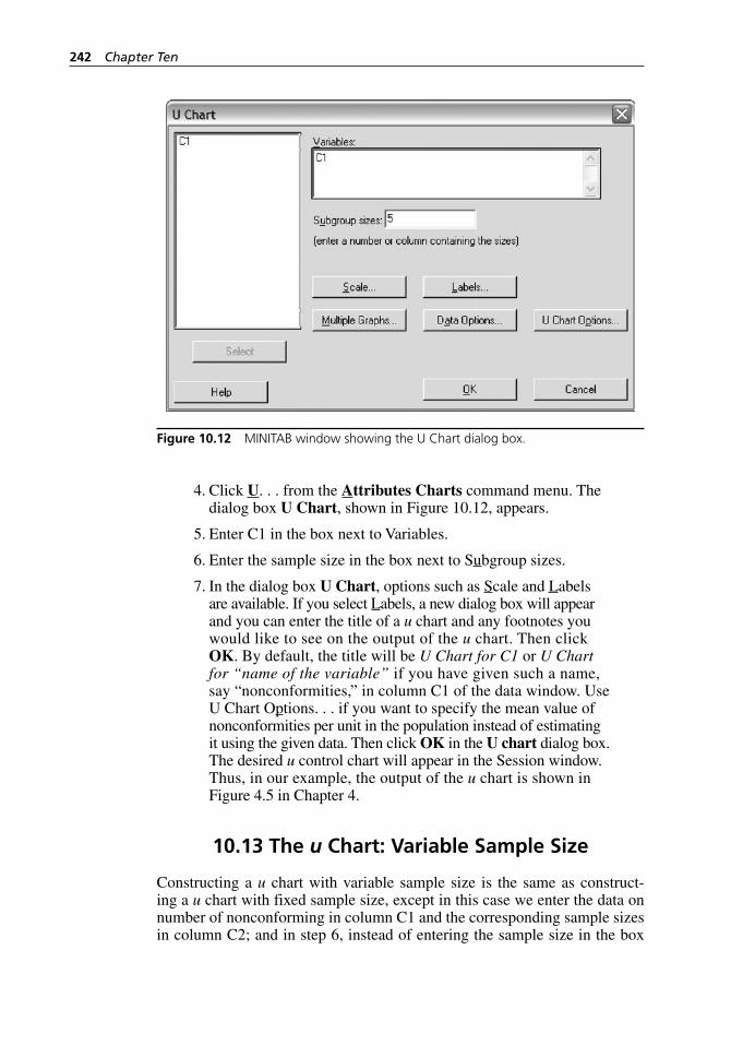
242 Chapter Ten
4. Click U. . . from the Attributes Charts command menu. The dialog box U Chart, shown in Figure 10.12, appears.
5. Enter C1 in the box next to Variables.
6. Enter the sample size in the box next to Subgroup sizes.
7. In the dialog box U Chart, options such as Scale and Labels are available. If you select Labels, a new dialog box will appear and you can enter the title of a u chart and any footnotes you would like to see on the output of the u chart. Then click OK. By default, the title will be U Chart for C1 or U Chart for “name of the variable” if you have given such a name, say “nonconformities,” in column C1 of the data window. Use U Chart Options. . . if you want to specify the mean value of nonconformities per unit in the population instead of estimating it using the given data. Then click OK in the U chart dialog box. The desired u control chart will appear in the Session window. Thus, in our example, the output of the u chart is shown in Figure 4.5 in Chapter 4.
10.13 The u Chart: Variable Sample Size
Constructing a u chart with variable sample size is the same as construct-ing a u chart with fixed sample size, except in this case we enter the data on number of nonconforming in column C1 and the corresponding sample sizes in column C2; and in step 6, instead of entering the sample size in the box
Figure 10.12 MINITAB window showing the U Chart dialog box.
H1277 ch10.indd 242H1277 ch10.indd 242 3/8/07 6:07:47 PM3/8/07 6:07:47 PM
Computer Resources to Support SQC: MINITAB 243
next to the Subgroup sizes, we enter C2. For an example of a u chart, see Figure 4.6 in Chapter 4.
10.14 Designing a CUSUM Control Chart
CUSUM charts are very effective in detecting small shifts. Unlike the X–
Shewhart control charts, CUSUM control charts can be designed to detect one-sided or two- sided shifts. These charts are defined by two parameters, k and h, which are called the reference value and the decision interval, respec-tively, and are defined in section 5.2.1. The two- sided process control by using a CUSUM control chart is achieved by concurrently using two one- sided CUSUM control charts. In both one- sided CUSUM charts one can use the same or different reference values depending on whether the upward and downward shifts are equally important. We discuss the construction of CUSUM control charts with the following example.
Example 10.9 Consider a manufacturing process of auto parts. We are interested in studying a quality characteristic of the parts manufactured by the process. Let the quality characteristic when the process is under control be normally distributed with mean 20 and standard deviation 2. The data shown in Table 5.1 of Example 5.1 in Chapter 5 give the first 10 random samples of size four, which are taken when the process is stable and pro-ducing the parts with mean value 20 and standard deviation 2. The last 10 random samples, again of size four, were taken from that process after its mean experienced an upward shift of one standard deviation, resulting in a new process with mean 22. Construct a Shewhart CUSUM control chart for the data in Table 5.1.
Solution:
1. Enter all the data in Table 5.1 of Chapter 5 in columns C1 through C4 (observations for each subgroup are entered in one row of columns) of the Worksheet window. Click Stat from the Menu Command.
2. Select Control Charts from the pull- down menu in the Stat command menu.
3. Select Time Weighted Charts from the Control Charts command menu.
4. Click CUSUM from the Control Charts command menu. The dialog box CUSUM Chart, shown in Figure 10.13, appears.
5. From the dialog box CUSUM Chart, choose the option “Observations for a subgroup are in one row of columns.”
6. Enter C1-C4 in the next box, because the sample size is four.
7. Enter the target value in the box next to Target, which in our example is 20.
H1277 ch10.indd 243H1277 ch10.indd 243 3/8/07 6:07:47 PM3/8/07 6:07:47 PM
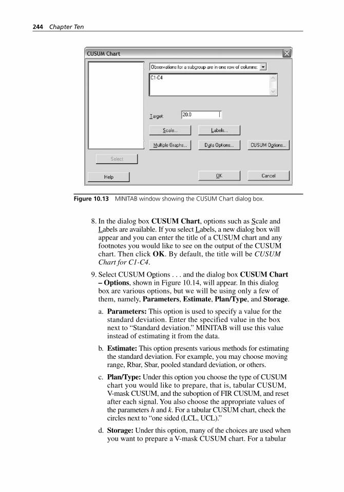
244 Chapter Ten
8. In the dialog box CUSUM Chart, options such as Scale and Labels are available. If you select Labels, a new dialog box will appear and you can enter the title of a CUSUM chart and any footnotes you would like to see on the output of the CUSUM chart. Then click OK. By default, the title will be CUSUM Chart for C1-C4.
9. Select CUSUM Options . . . and the dialog box CUSUM Chart – Options, shown in Figure 10.14, will appear. In this dialog box are various options, but we will be using only a few of them, namely, Parameters, Estimate, Plan/Type, and Storage.
a. Parameters: This option is used to specify a value for the standard deviation. Enter the specified value in the box next to “Standard deviation.” MINITAB will use this value instead of estimating it from the data.
b. Estimate: This option presents various methods for estimating the standard deviation. For example, you may choose moving range, Rbar, Sbar, pooled standard deviation, or others.
c. Plan/Type: Under this option you choose the type of CUSUM chart you would like to prepare, that is, tabular CUSUM, V-mask CUSUM, and the suboption of FIR CUSUM, and reset after each signal. You also choose the appropriate values of the parameters h and k. For a tabular CUSUM chart, check the circles next to “one sided (LCL, UCL).”
d. Storage: Under this option, many of the choices are used when you want to prepare a V-mask CUSUM chart. For a tabular
Figure 10.13 MINITAB window showing the CUSUM Chart dialog box.
H1277 ch10.indd 244H1277 ch10.indd 244 3/8/07 6:07:47 PM3/8/07 6:07:47 PM
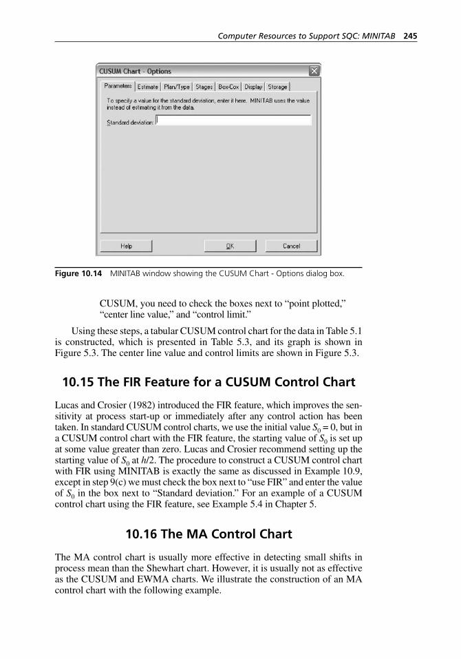
Computer Resources to Support SQC: MINITAB 245
CUSUM, you need to check the boxes next to “point plotted,” “center line value,” and “control limit.”
Using these steps, a tabular CUSUM control chart for the data in Table 5.1 is constructed, which is presented in Table 5.3, and its graph is shown in Figure 5.3. The center line value and control limits are shown in Figure 5.3.
10.15 The FIR Feature for a CUSUM Control Chart
Lucas and Crosier (1982) introduced the FIR feature, which improves the sen-sitivity at process start- up or immediately after any control action has been taken. In standard CUSUM control charts, we use the initial value S0 = 0, but in a CUSUM control chart with the FIR feature, the starting value of S0 is set up at some value greater than zero. Lucas and Crosier recommend setting up the starting value of S0 at h/2. The procedure to construct a CUSUM control chart with FIR using MINITAB is exactly the same as discussed in Example 10.9, except in step 9(c) we must check the box next to “use FIR” and enter the value of S0 in the box next to “Standard deviation.” For an example of a CUSUM control chart using the FIR feature, see Example 5.4 in Chapter 5.
10.16 The MA Control Chart
The MA control chart is usually more effective in detecting small shifts in process mean than the Shewhart chart. However, it is usually not as effective as the CUSUM and EWMA charts. We illustrate the construction of an MA control chart with the following example.
Figure 10.14 MINITAB window showing the CUSUM Chart - Options dialog box.
H1277 ch10.indd 245H1277 ch10.indd 245 3/8/07 6:07:47 PM3/8/07 6:07:47 PM
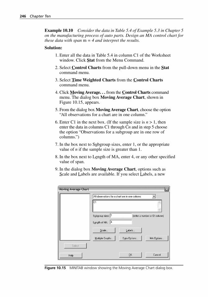
246 Chapter Ten
Example 10.10 Consider the data in Table 5.4 of Example 5.3 in Chapter 5 on the manufacturing process of auto parts. Design an MA control chart for these data with span m = 4 and interpret the results.
Solution:
1. Enter all the data in Table 5.4 in column C1 of the Worksheet window. Click Stat from the Menu Command.
2. Select Control Charts from the pull- down menu in the Stat command menu.
3. Select Time Weighted Charts from the Control Charts command menu.
4. Click Moving Average. . . from the Control Charts command menu. The dialog box Moving Average Chart, shown in Figure 10.15, appears.
5. From the dialog box Moving Average Chart, choose the option “All observations for a chart are in one column.”
6. Enter C1 in the next box. (If the sample size is n > 1, then enter the data in columns C1 through Cn and in step 5 choose the option “Observations for a subgroup are in one row of columns.”)
7. In the box next to Subgroup sizes, enter 1, or the appropriate value of n if the sample size is greater than 1.
8. In the box next to Length of MA, enter 4, or any other specified value of span.
9. In the dialog box Moving Average Chart, options such as Scale and Labels are available. If you select Labels, a new
Figure 10.15 MINITAB window showing the Moving Average Chart dialog box.
H1277 ch10.indd 246H1277 ch10.indd 246 3/8/07 6:07:47 PM3/8/07 6:07:47 PM
Computer Resources to Support SQC: MINITAB 247
dialog box will appear and you can enter the title of a Moving Average chart and any footnotes that you would like to see on the output of the Moving Average chart. Then click OK. By default, the title will be Moving Average Chart for C1.
10. Select MA Options . . . and the dialog box Moving Average Chart – Options will appear. In this dialog box are various options, but we will be using only a few of them, namely, Parameters, Estimate, S Limits, and Storage.
a. Parameters: This option is used to specify a value of the mean and a value of the standard deviation. Enter the specified values in the boxes next to “Mean” and “Standard deviation.” MINITAB will use this value instead of estimating it from the data.
b. Estimate: This option presents various methods for estimating the mean and the standard deviation. For example, you may choose moving range, Rbar, Sbar, and others.
c. S Limits: Under this option you choose, for example, control limits, bounds on control limits, and sample size.
d. Storage: Under this option, check the boxes next to “point plotted,” “center line value,” and “control limit” and then click OK. Finally, click OK in the Moving Average Chart dialog box.
Using these steps, the MA control chart for the data in Table 5.4 is con-structed. It is presented in Table 5.7, and its graph is shown in Figure 5.7. The center line value and control limits are shown in Figure 5.7.
10.17 The EWMA Control Chart
The EWMA control chart is very useful for processes in which only one observation per period may be available. We discuss the construction of an EWMA control chart using MINITAB with the following example.
Example 10.11 Consider the data in Table 5.4 of Example 5.3 in Chapter 5 on the manufacturing process of auto parts. Design an EWMA control chart for these data with λ = 0.20, L = 2.962, µ0 = 20, and σ = 2 and interpret the results.
Solution:
1. Enter all the data in Table 5.4 in column C1 of the Worksheet window. Click Stat from the Menu Command.
2. Select Control Charts from the pull- down menu in the Stat command menu.
3. Select Time Weighted Charts from the Control Charts command menu.
H1277 ch10.indd 247H1277 ch10.indd 247 3/8/07 6:07:48 PM3/8/07 6:07:48 PM
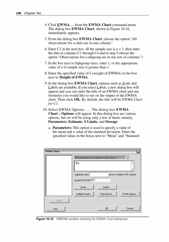
248 Chapter Ten
4. Click EWMA. . . from the EWMA Chart command menu. The dialog box EWMA Chart, shown in Figure 10.16, immediately appears.
5. From the dialog box EWMA Chart, choose the option “All observations for a chart are in one column.”
6. Enter C1 in the next box. (If the sample size is n > 1, then enter the data in columns C1 through Cn and in step 5 choose the option “Observations for a subgroup are in one row of columns.”)
7. In the box next to Subgroup sizes, enter 1, or the appropriate value of n if sample size is greater than 1.
8. Enter the specified value of λ (weight of EWMA) in the box next to Weight of EWMA.
9. In the dialog box EWMA Chart, options such as Scale and Labels are available. If you select Labels, a new dialog box will appear and you can enter the title of an EWMA chart and any footnotes you would like to see on the output of the EWMA chart. Then click OK. By default, the title will be EWMA Chart for C1.
10. Select EWMA Options. . . . The dialog box EWMA Chart – Options will appear. In this dialog box are various options, but we will be using only a few of them, namely, Parameters, Estimate, S Limits, and Storage.
a. Parameters: This option is used to specify a value of the mean and a value of the standard deviation. Enter the specified values in the boxes next to “Mean” and “Standard
Figure 10.16 MINITAB window showing the EWMA Chart dialog box.
H1277 ch10.indd 248H1277 ch10.indd 248 3/8/07 6:07:48 PM3/8/07 6:07:48 PM
Computer Resources to Support SQC: MINITAB 249
deviation.” MINITAB will use this value instead of estimating it from the data.
b. Estimate: This option presents various methods for estimating the standard deviation. For example, you may choose Average moving range, Rbar, Sbar, Pooled standard deviation, or others.
c. S Limits: Under this option you choose, for example, Display control limits, bounds on control limits, and sample size. In this example, under the option Display control limits, enter the value of L = 2.962 in the box next to “These multiples of the standard deviation.”
d. Storage: Under this option, check the boxes next to “point plotted,” “center line value,” and “control limit” and then click OK. Finally, click OK in the EWMA Chart dialog box.
Using these steps, the EWMA control chart for the data in Table 5.4 is con-structed. It is presented in Table 5.9, and its graph is shown in Figure 5.8. The center line value and control limits are shown in Figure 5.8.
10.18 Measurement System Capability Analysis
The measurement system plays an important role in any effort to improve a process. In any process, the total process variation consists of two sources:
Part-to-part variation
Measurement system variation
If the measurement system variation is large compared with part- to-part variation, the measurement system cannot adequately discriminate between parts for complete process evaluation. In other words, the measurement sys-tem is not capable. It becomes very important to perform measurement sys-tem capability analysis.
Suppose we measure a quality characteristic of a part and let t be the total observed value of the quality characteristic, p be its true value, and e be the measurement error. Then, we have
t = p + e. (10.1)
Assume now that the true value of the quality characteristic and the measure-ment error are normally distributed with mean µ and 0 and variances σ p
2 and σm
2 , respectively. Then it can be shown that
σ σ σt p m
2 2 2= + , (10.2)
where σ t2 is the variance of the total observed values. Furthermore, the error
variance σm2 usually consists of two components: one due to gage variation
(repeatability) and the other due to operator variation (reproducibility). The
•
•
H1277 ch10.indd 249H1277 ch10.indd 249 3/8/07 6:07:48 PM3/8/07 6:07:48 PM
250 Chapter Ten
purpose of measurement system capability analysis is to separate these com-ponents and analyze them. In other words, we have
σ σ σmeasurement error reproducibilty repeat
2 2= + aability2 .
To study these components, we usually use the ANOVA technique, which is also known as Gage R&R study. When using the ANOVA technique, we commonly deal with two types of situations: (1) when each operator measures the same specimens of a part, and (2) when each operator measures different specimens of a part. The designs used under these situations are known as crossed and nested designs, respectively. The following section discusses the Gage R&R study using MINITAB and crossed designs. We do not discuss nested designs here, as they are beyond the scope of this book.
10.18.1 Measurement System Capability Analysis (Using Crossed Designs)
A manufacturer of tubes used in automotive applications has installed a new measuring gage. The Six Sigma Green Belt team is interested in determining how well the new gage measures the inside diameter of the tube. In other words, the team is interested in performing the measurement system capabil-ity analysis. We discuss the measurement system capability analysis with the following example.
Example 10.12 A manufacturer of bolts (parts) used in automotive applications has installed a new measuring gage. In order to perform the MSA on the new gage, the quality manager randomly selects three Six Sigma Green Belts from the quality control department, who decide to take a ran-dom sample of 10 bolts. Each Six Sigma Green Belt takes three measurements on each bolt, which is selected randomly. The data obtained are shown in Table 10.2.
Estimate the repeatability and reproducibility of the measurement system.
Estimate how much of the total process variation is due to the mea-surement system.
If the tube diameter specifications are 70 ± 10, what can we say about the discrimination power of the measurement system? In other words, is the measurement system capable of discriminating between different parts?
Solution: We have already discussed this example earlier, in Chapter 7. Here we discuss step by step how to set up MINITAB to find the solution to this or any other similar problem.
1. Following the steps discussed in section 10.1, start up MINITAB. The screen titled MINITAB – UNTITLED will appear first.
•
•
•
H1277 ch10.indd 250H1277 ch10.indd 250 3/8/07 6:07:48 PM3/8/07 6:07:48 PM
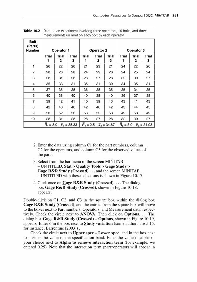
Computer Resources to Support SQC: MINITAB 251
2. Enter the data using column C1 for the part numbers, column C2 for the operators, and column C3 for the observed values of the parts.
3. Select from the bar menu of the screen MINITAB – UNTITLED, Stat > Quality Tools > Gage Study > Gage R&R Study (Crossed) . . . and the screen MINITAB – UNTITLED with these selections is shown in Figure 10.17.
4. Click once on Gage R&R Study (Crossed). . . . The dialog box Gage R&R Study (Crossed), shown in Figure 10.18, appears.
Double-click on C1, C2, and C3 in the square box within the dialog box Gage R&R Study (Crossed), and the entries from the square box will move to the boxes next to Part numbers, Operators, and Measurement data, respec-tively. Check the circle next to ANOVA. Then click on Options. . .. The dialog box Gage R&R Study (Crossed) – Options, shown in Figure 10.19, appears. Enter 6 in the box next to Study variation (some authors use 5.15, for instance, Barrentine [2003]) .
Check the circle next to Upper spec – Lower spec, and in the box next to it enter the value of the specification band. Enter the value of alpha of your choice next to Alpha to remove interaction term (for example, we entered 0.25). Note that the interaction term (part*operator) will appear in
Table 10.2 Data on an experiment involving three operators, 10 bolts, and three measurements (in mm) on each bolt by each operator.
Bolt (Parts)
Number Operator 1 Operator 2 Operator 3
Trial 1
Trial 2
Trial 3
Trial 1
Trial 2
Trial 3
Trial 1
Trial 2
Trial 3
1 26 22 26 21 23 21 24 22 26
2 28 26 28 24 29 26 24 25 24
3 28 31 28 28 27 28 32 30 27
4 35 33 31 35 31 30 34 35 31
5 37 35 38 36 38 35 35 34 35
6 40 38 40 40 38 40 36 37 38
7 39 42 41 40 39 43 43 41 43
8 42 43 46 42 46 42 43 44 45
9 50 52 50 53 52 53 49 53 49
10 28 31 28 28 27 28 32 30 27
R–
1 = 3.0 x–1 = 35.33 R–
2 = 2.5 x–2 = 34.67 R–
3 = 3.0 x–3 = 34.93
H1277 ch10.indd 251H1277 ch10.indd 251 3/8/07 6:07:48 PM3/8/07 6:07:48 PM
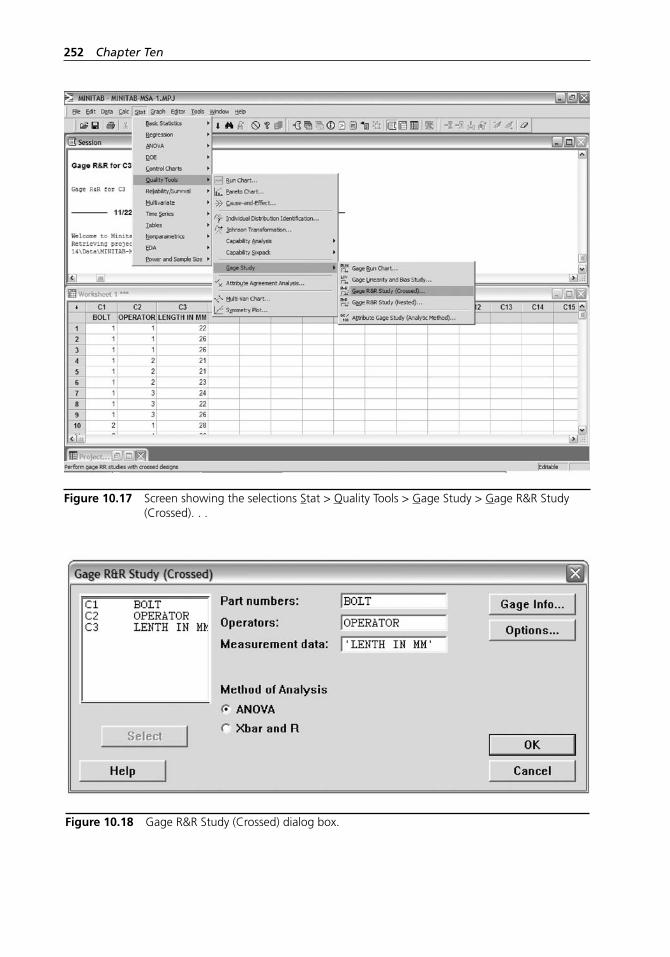
252 Chapter Ten
Figure 10.17 Screen showing the selections Stat > Quality Tools > Gage Study > Gage R&R Study (Crossed). . .
Figure 10.18 Gage R&R Study (Crossed) dialog box.
H1277 ch10.indd 252H1277 ch10.indd 252 3/8/07 6:07:49 PM3/8/07 6:07:49 PM
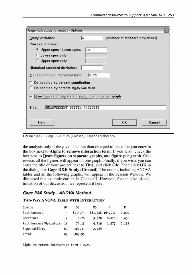
Computer Resources to Support SQC: MINITAB 253
the analysis only if the p value is less than or equal to the value you enter in the box next to Alpha to remove interaction term. If you wish, check the box next to Draw figures on separate graphs, one figure per graph. Oth-erwise, all the figures will appear on one graph. Finally, if you wish, you can enter the title of your project next to Title, and click OK. Then click OK in the dialog box Gage R&R Study (Crossed). The output, including ANOVA tables and all the following graphs, will appear in the Session Window. We discussed this example earlier, in Chapter 7. However, for the sake of con-tinuation of our discussion, we represent it here.
Gage R&R Study—ANOVA Method
Two-Way ANOVA Table with Interaction
Source DF SS MS F P
Part Numbers 9 6135.73 681.748 165.532 0.000
Operators 2 6.76 3.378 0.820 0.456
Part Numbers*Operators 18 74.13 4.119 1.477 0.131
Repeatability 60 167.33 2.789
Total 89 6383.95
Alpha to remove interaction term = 0.25
Figure 10.19 Gage R&R Study (Crossed) - Options dialog box.
H1277 ch10.indd 253H1277 ch10.indd 253 3/8/07 6:07:49 PM3/8/07 6:07:49 PM
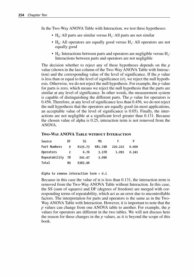
254 Chapter Ten
In the Two- Way ANOVA Table with Interaction, we test three hypotheses:
H0: All parts are similar versus H1: All parts are not similar
H0: All operators are equally good versus H1: All operators are not equally good
H0: Interactions between parts and operators are negligible versus H1: Interactions between parts and operators are not negligible
The decision whether to reject any of these hypotheses depends on the p value (shown in the last column of the Two- Way ANOVA Table with Interac-tion) and the corresponding value of the level of significance. If the p value is less than or equal to the level of significance (σ), we reject the null hypoth-esis. Otherwise, we do not reject the null hypothesis. For example, the p value for parts is zero, which means we reject the null hypothesis that the parts are similar at any level of significance. In other words, the measurement system is capable of distinguishing the different parts. The p value for operators is 0.456. Therefore, at any level of significance less than 0.456, we do not reject the null hypothesis that the operators are equally good (in most applications, an acceptable value of the level of significance is 0.05). Finally, the inter-actions are not negligible at a significant level greater than 0.131. Because the chosen value of alpha is 0.25, interaction term is not removed from the ANOVA.
Two-Way ANOVA Table without Interaction
Source DF SS MS F P
Part Numbers 9 6135.73 681.748 220.222 0.000
Operators 2 6.76 3.378 1.091 0.341
Repeatability 78 241.47 3.096
Total 89 6383.96
Alpha to remove interaction term = 0.1
Because in this case the value of α is less than 0.131, the interaction term is removed from the Two- Way ANOVA Table without Interaction. In this case, the SS (sum of squares) and DF (degrees of freedom) are merged with cor-responding terms of repeatability, which act as an error due to uncontrollable factors. The interpretation for parts and operators is the same as in the Two- Way ANOVA Table with Interaction. However, it is important to note that the p values can change from one ANOVA table to another. For example, the p values for operators are different in the two tables. We will not discuss here the reason for these changes in the p values, as it is beyond the scope of this book.
•
•
•
H1277 ch10.indd 254H1277 ch10.indd 254 3/8/07 6:07:49 PM3/8/07 6:07:49 PM
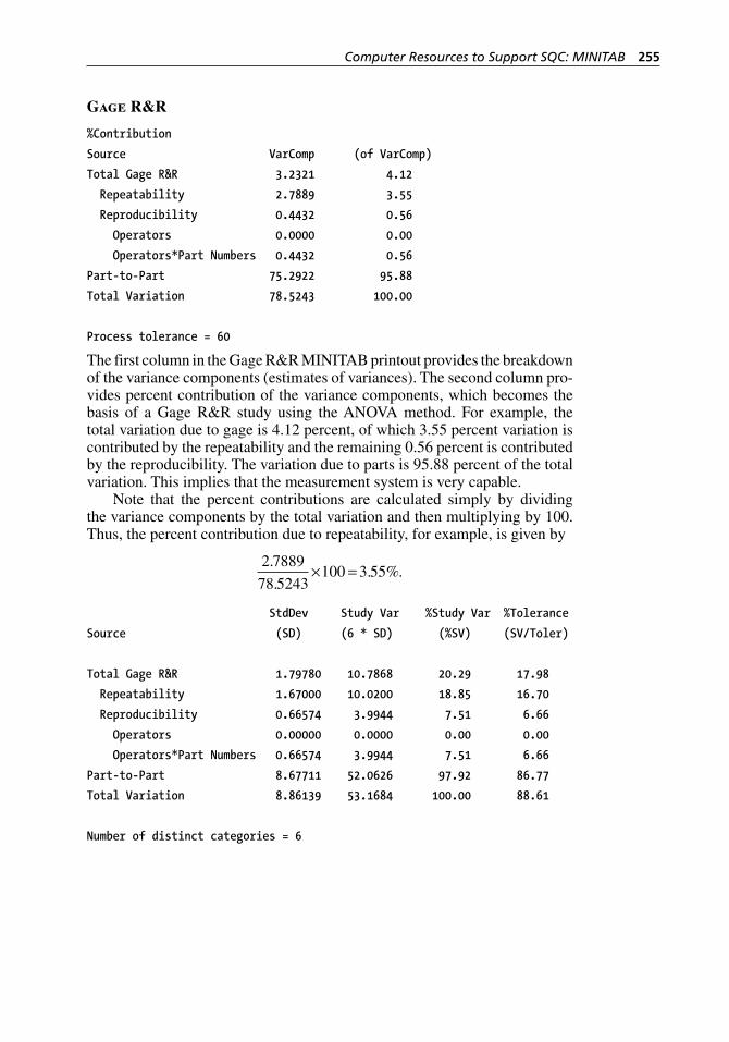
Computer Resources to Support SQC: MINITAB 255
Gage R&R
%Contribution
Source VarComp (of VarComp)
Total Gage R&R 3.2321 4.12
Repeatability 2.7889 3.55
Reproducibility 0.4432 0.56
Operators 0.0000 0.00
Operators*Part Numbers 0.4432 0.56
Part-to-Part 75.2922 95.88
Total Variation 78.5243 100.00
Process tolerance = 60
The first column in the Gage R&R MINITAB printout provides the breakdown of the variance components (estimates of variances). The second column pro-vides percent contribution of the variance components, which becomes the basis of a Gage R&R study using the ANOVA method. For example, the total variation due to gage is 4.12 percent, of which 3.55 percent variation is contributed by the repeatability and the remaining 0.56 percent is contributed by the reproducibility. The variation due to parts is 95.88 percent of the total variation. This implies that the measurement system is very capable.
Note that the percent contributions are calculated simply by dividing the variance components by the total variation and then multiplying by 100. Thus, the percent contribution due to repeatability, for example, is given by
2 7889
78 5243100 3 55
.
.. %.× =
StdDev Study Var %Study Var %Tolerance
Source (SD) (6 * SD) (%SV) (SV/Toler)
Total Gage R&R 1.79780 10.7868 20.29 17.98
Repeatability 1.67000 10.0200 18.85 16.70
Reproducibility 0.66574 3.9944 7.51 6.66
Operators 0.00000 0.0000 0.00 0.00
Operators*Part Numbers 0.66574 3.9944 7.51 6.66
Part-to-Part 8.67711 52.0626 97.92 86.77
Total Variation 8.86139 53.1684 100.00 88.61
Number of distinct categories = 6
H1277 ch10.indd 255H1277 ch10.indd 255 3/8/07 6:07:49 PM3/8/07 6:07:49 PM
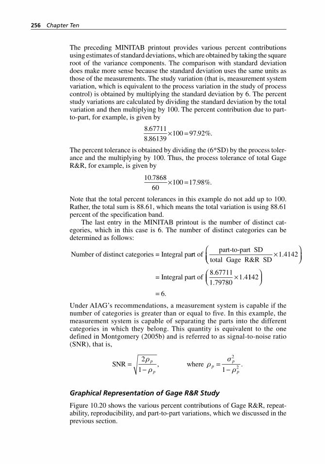
256 Chapter Ten
The preceding MINITAB printout provides various percent contributions using estimates of standard deviations, which are obtained by taking the square root of the variance components. The comparison with standard deviation does make more sense because the standard deviation uses the same units as those of the measurements. The study variation (that is, measurement system variation, which is equivalent to the process variation in the study of process control) is obtained by multiplying the standard deviation by 6. The percent study variations are calculated by dividing the standard deviation by the total variation and then multiplying by 100. The percent contribution due to part- to-part, for example, is given by
8 67711
8 86139100 97 92
.
.. %.× =
The percent tolerance is obtained by dividing the (6*SD) by the process toler-ance and the multiplying by 100. Thus, the process tolerance of total Gage R&R, for example, is given by
10 7868
60100 17 98
.. %.× =
Note that the total percent tolerances in this example do not add up to 100. Rather, the total sum is 88.61, which means the total variation is using 88.61 percent of the specification band.
The last entry in the MINITAB printout is the number of distinct cat-egories, which in this case is 6. The number of distinct categories can be determined as follows:
Number of distinct categories = Integral parrt ofpart-to-part SD
total Gage R&R SD×
⎛1 4142.
⎝⎝⎜⎞⎠⎟
×= Integral part of8 67711
1 797801 4
.
.. 1142
6
⎛⎝⎜
⎞⎠⎟
= .
Under AIAG’s recommendations, a measurement system is capable if the number of categories is greater than or equal to five. In this example, the measurement system is capable of separating the parts into the different categories in which they belong. This quantity is equivalent to the one defined in Montgomery (2005b) and is referred to as signal- to-noise ratio (SNR), that is,
SNR where=−
=−
2
1 1
2
2
ρ
ρρ
σ
ρp
pp
p
p
, .
Graphical Representation of Gage R&R Study
Figure 10.20 shows the various percent contributions of Gage R&R, repeat-ability, reproducibility, and part- to-part variations, which we discussed in the previous section.
H1277 ch10.indd 256H1277 ch10.indd 256 3/8/07 6:07:49 PM3/8/07 6:07:49 PM
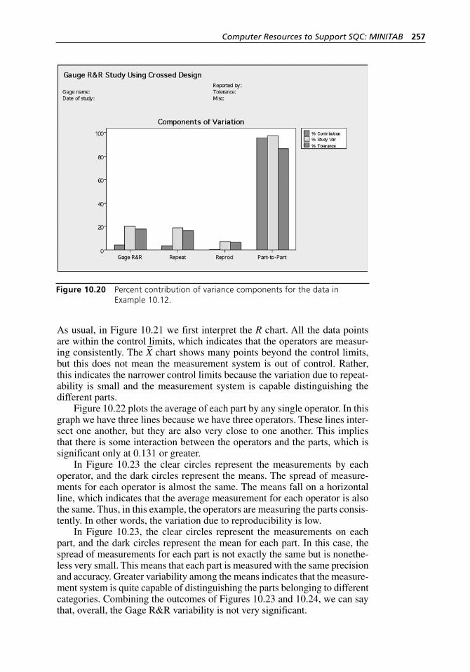
Computer Resources to Support SQC: MINITAB 257
As usual, in Figure 10.21 we first interpret the R chart. All the data points are within the control limits, which indicates that the operators are measur-ing consistently. The X
– chart shows many points beyond the control limits,
but this does not mean the measurement system is out of control. Rather, this indicates the narrower control limits because the variation due to repeat-ability is small and the measurement system is capable distinguishing the different parts.
Figure 10.22 plots the average of each part by any single operator. In this graph we have three lines because we have three operators. These lines inter-sect one another, but they are also very close to one another. This implies that there is some interaction between the operators and the parts, which is significant only at 0.131 or greater.
In Figure 10.23 the clear circles represent the measurements by each operator, and the dark circles represent the means. The spread of measure-ments for each operator is almost the same. The means fall on a horizontal line, which indicates that the average measurement for each operator is also the same. Thus, in this example, the operators are measuring the parts consis-tently. In other words, the variation due to reproducibility is low.
In Figure 10.23, the clear circles represent the measurements on each part, and the dark circles represent the mean for each part. In this case, the spread of measurements for each part is not exactly the same but is nonethe-less very small. This means that each part is measured with the same precision and accuracy. Greater variability among the means indicates that the measure-ment system is quite capable of distinguishing the parts belonging to different categories. Combining the outcomes of Figures 10.23 and 10.24, we can say that, overall, the Gage R&R variability is not very significant.
Figure 10.20 Percent contribution of variance components for the data in Example 10.12.
H1277 ch10.indd 257H1277 ch10.indd 257 3/8/07 6:07:49 PM3/8/07 6:07:49 PM
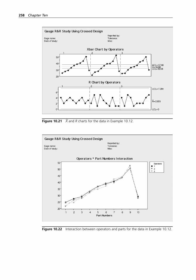
258 Chapter Ten
Figure 10.21 X– and R charts for the data in Example 10.12.
Figure 10.22 Interaction between operators and parts for the data in Example 10.12.
H1277 ch10.indd 258H1277 ch10.indd 258 3/8/07 6:07:50 PM3/8/07 6:07:50 PM
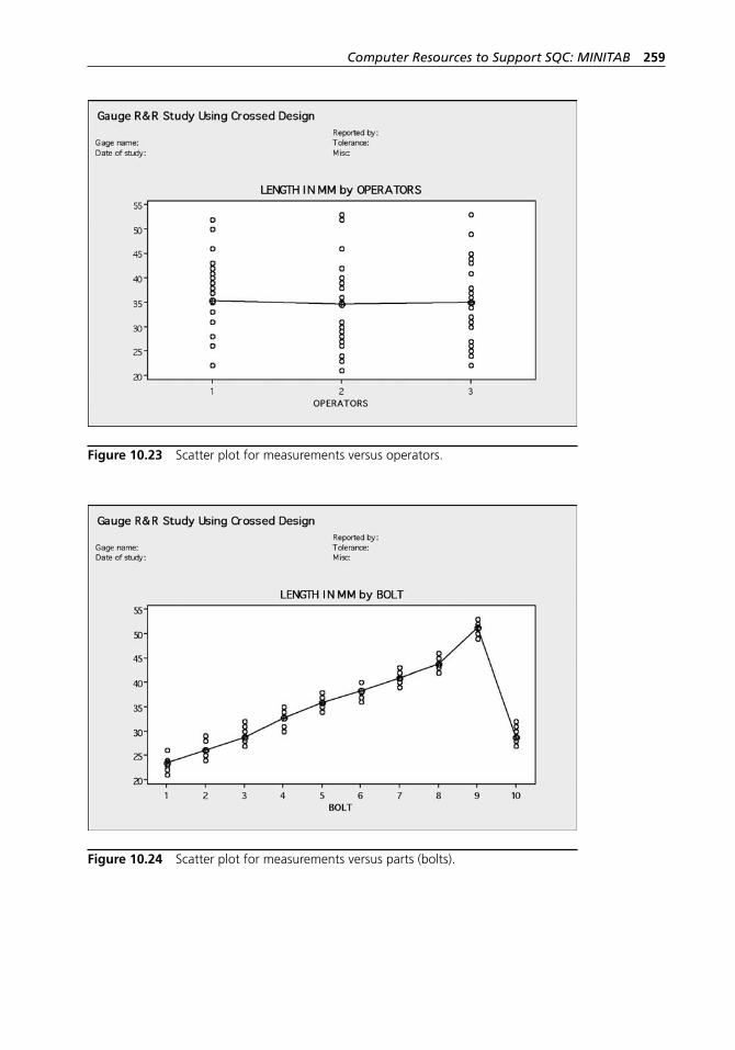
Computer Resources to Support SQC: MINITAB 259
Figure 10.23 Scatter plot for measurements versus operators.
Figure 10.24 Scatter plot for measurements versus parts (bolts).
H1277 ch10.indd 259H1277 ch10.indd 259 3/8/07 6:07:50 PM3/8/07 6:07:50 PM

H1277 ch10.indd 260H1277 ch10.indd 260 3/8/07 6:07:50 PM3/8/07 6:07:50 PM

261
Use of all the SQC tools discussed in this book began with hand calcu-lation. Aside from the tediousness of the calculations, data transcrip-tion, and calculation errors, the amount of time required to complete
the calculations and related graphing drove the need for computer support of SQC applications. Now there are many desktop statistical application soft-ware packages available to support SQC, and the focus of this chapter is on one of those software packages: JMP. In this chapter we will limit our discus-sion of topics to demonstrating the use of JMP for the tools and techniques discussed throughout this book, and we will emphasize the use of JMP for phase I and II SPC charts, process capability, and MSA. We will not discuss the use of JMP for acceptance sampling or PRE- control, as JMP is not spe-cifically designed in Version 6.0 to support these SQC tools and techniques.
It is not our intent as authors to endorse any one software package, as each package has particular strengths and areas for improvement. We do, however, feel the need to introduce JMP as a software package that is very popular, that is statistically very powerful, and that supports the statistical content discussed in each of the four books in the Six Sigma Green Belt series. In order to gain the most benefit from the material in this chapter, readers should have basic computing literacy.
11.1 Using JMP—Version 6.0
When launching JMP, you will see the screen shown in Figure 11.1, which identifies JMP Starter as the topmost heading, indicating that there are no open files. Immediately below the drop- down menu is a dialog box, also with the heading of JMP Starter.
The JMP Starter is designed to assist new(er) JMP users by providing easily accessible prompts for and brief descriptions of the most common functions needed to start a JMP session. The JMP Starter is organized around categories of functions whereby you can select any of the categories of func-tions listed on the left side of Figure 11.1. The current category displayed is File, and the functions corresponding to the File category are shown in
11
Computer Resources to Support SQC: JMP
H1277 ch11.indd 261H1277 ch11.indd 261 3/8/07 12:39:47 PM3/8/07 12:39:47 PM
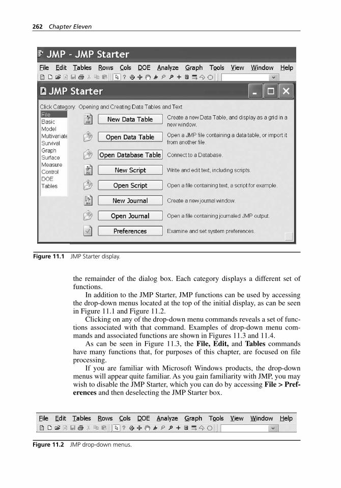
262 Chapter Eleven
the remainder of the dialog box. Each category displays a different set of functions.
In addition to the JMP Starter, JMP functions can be used by accessing the drop- down menus located at the top of the initial display, as can be seen in Figure 11.1 and Figure 11.2.
Clicking on any of the drop- down menu commands reveals a set of func-tions associated with that command. Examples of drop- down menu com-mands and associated functions are shown in Figures 11.3 and 11.4.
As can be seen in Figure 11.3, the File, Edit, and Tables commands have many functions that, for purposes of this chapter, are focused on file processing.
If you are familiar with Microsoft Windows products, the drop- down menus will appear quite familiar. As you gain familiarity with JMP, you may wish to disable the JMP Starter, which you can do by accessing File > Pref-erences and then deselecting the JMP Starter box.
Figure 11.1 JMP Starter display.
Figure 11.2 JMP drop- down menus.
H1277 ch11.indd 262H1277 ch11.indd 262 3/8/07 12:39:48 PM3/8/07 12:39:48 PM
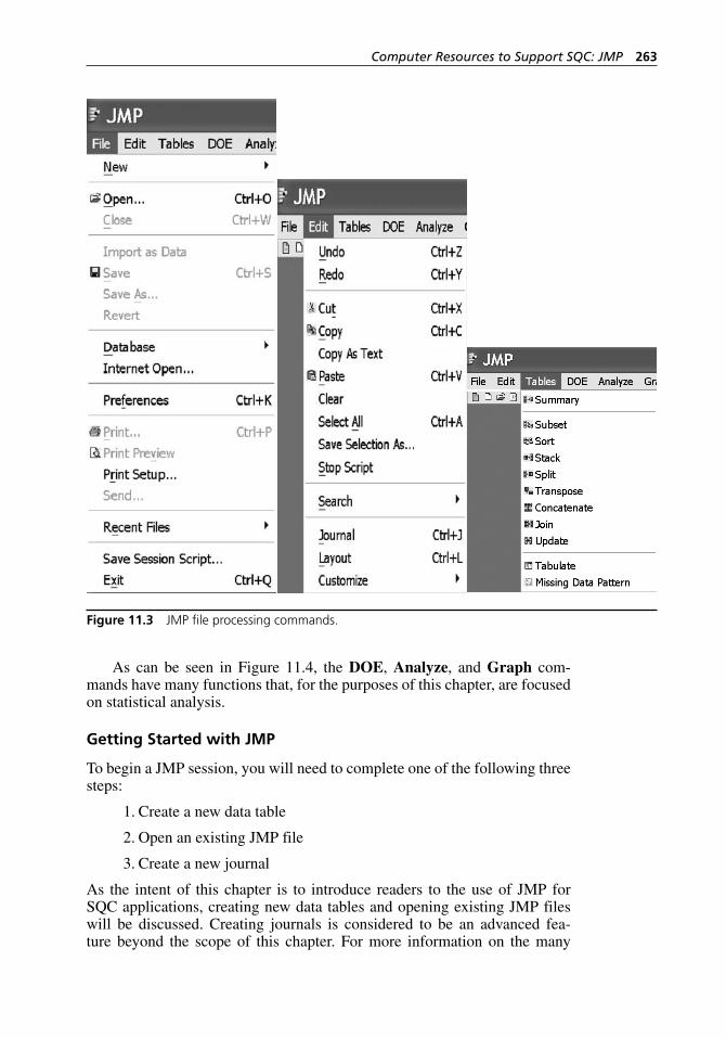
Computer Resources to Support SQC: JMP 263
As can be seen in Figure 11.4, the DOE, Analyze, and Graph com-mands have many functions that, for the purposes of this chapter, are focused on statistical analysis.
Getting Started with JMP
To begin a JMP session, you will need to complete one of the following three steps:
1. Create a new data table
2. Open an existing JMP file
3. Create a new journal
As the intent of this chapter is to introduce readers to the use of JMP for SQC applications, creating new data tables and opening existing JMP files will be discussed. Creating journals is considered to be an advanced fea-ture beyond the scope of this chapter. For more information on the many
Figure 11.3 JMP file processing commands.
H1277 ch11.indd 263H1277 ch11.indd 263 3/8/07 12:39:48 PM3/8/07 12:39:48 PM
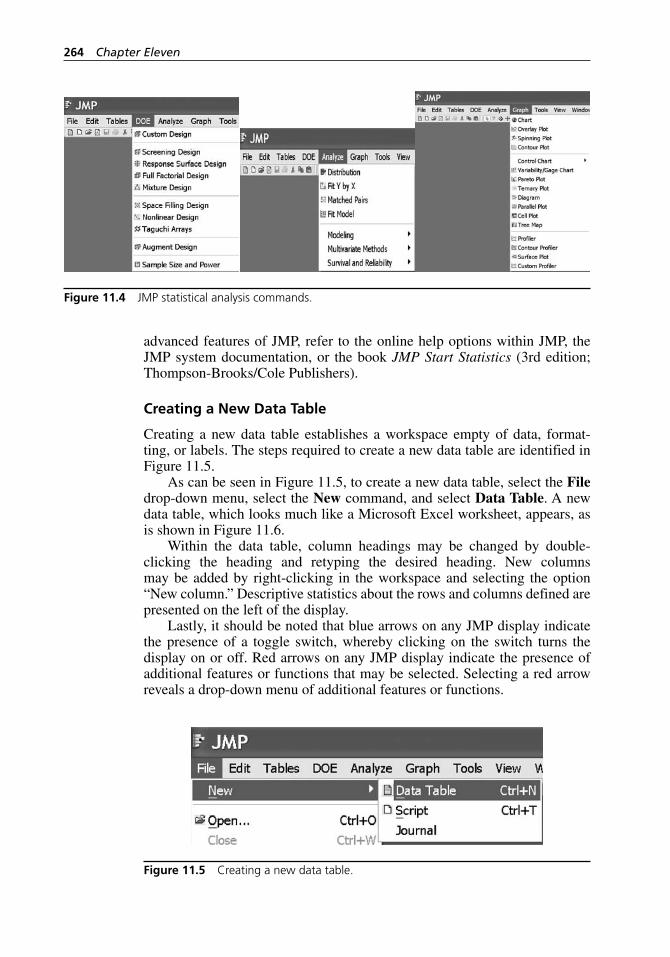
264 Chapter Eleven
advanced features of JMP, refer to the online help options within JMP, the JMP system documentation, or the book JMP Start Statistics (3rd edition; Thompson- Brooks/Cole Publishers).
Creating a New Data Table
Creating a new data table establishes a workspace empty of data, format-ting, or labels. The steps required to create a new data table are identified in Figure 11.5.
As can be seen in Figure 11.5, to create a new data table, select the File drop- down menu, select the New command, and select Data Table. A new data table, which looks much like a Microsoft Excel worksheet, appears, as is shown in Figure 11.6.
Within the data table, column headings may be changed by double- clicking the heading and retyping the desired heading. New columns may be added by right- clicking in the workspace and selecting the option “New column.” Descriptive statistics about the rows and columns defined are presented on the left of the display.
Lastly, it should be noted that blue arrows on any JMP display indicate the presence of a toggle switch, whereby clicking on the switch turns the display on or off. Red arrows on any JMP display indicate the presence of additional features or functions that may be selected. Selecting a red arrow reveals a drop- down menu of additional features or functions.
Figure 11.4 JMP statistical analysis commands.
Figure 11.5 Creating a new data table.
H1277 ch11.indd 264H1277 ch11.indd 264 3/8/07 12:39:49 PM3/8/07 12:39:49 PM
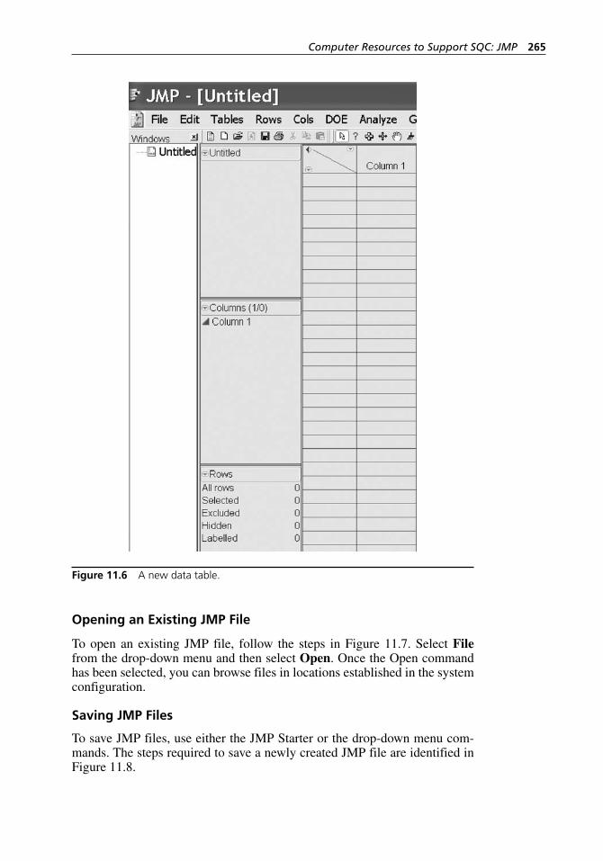
Computer Resources to Support SQC: JMP 265
Figure 11.6 A new data table.
Opening an Existing JMP File
To open an existing JMP file, follow the steps in Figure 11.7. Select File from the drop- down menu and then select Open. Once the Open command has been selected, you can browse files in locations established in the system configuration.
Saving JMP Files
To save JMP files, use either the JMP Starter or the drop- down menu com-mands. The steps required to save a newly created JMP file are identified in Figure 11.8.
H1277 ch11.indd 265H1277 ch11.indd 265 3/8/07 12:39:49 PM3/8/07 12:39:49 PM
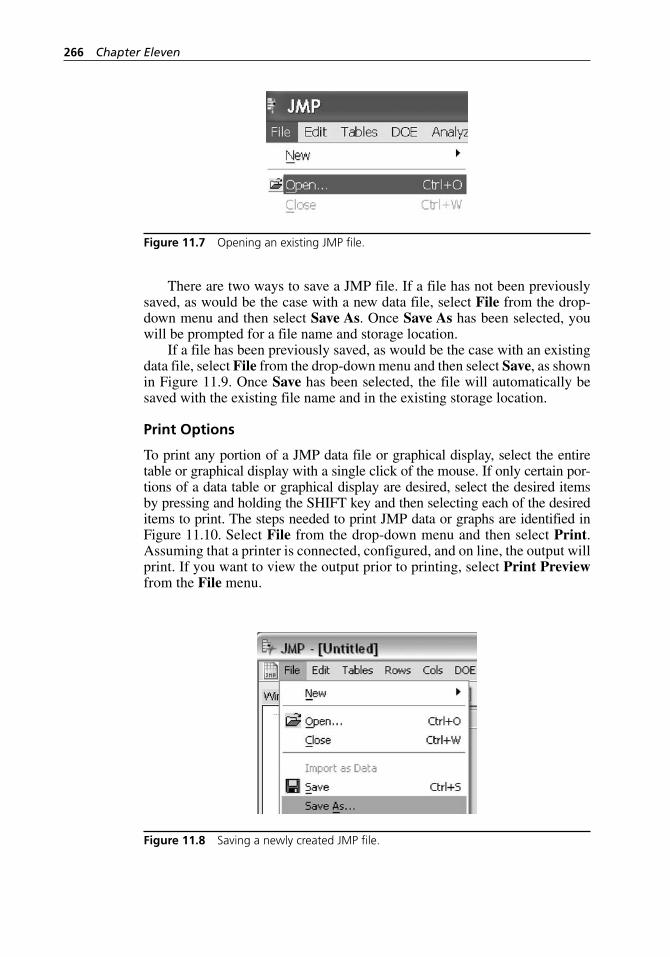
266 Chapter Eleven
There are two ways to save a JMP file. If a file has not been previously saved, as would be the case with a new data file, select File from the drop- down menu and then select Save As. Once Save As has been selected, you will be prompted for a file name and storage location.
If a file has been previously saved, as would be the case with an existing data file, select File from the drop- down menu and then select Save, as shown in Figure 11.9. Once Save has been selected, the file will automatically be saved with the existing file name and in the existing storage location.
Print Options
To print any portion of a JMP data file or graphical display, select the entire table or graphical display with a single click of the mouse. If only certain por-tions of a data table or graphical display are desired, select the desired items by pressing and holding the SHIFT key and then selecting each of the desired items to print. The steps needed to print JMP data or graphs are identified in Figure 11.10. Select File from the drop- down menu and then select Print. Assuming that a printer is connected, configured, and on line, the output will print. If you want to view the output prior to printing, select Print Preview from the File menu.
Figure 11.8 Saving a newly created JMP file.
Figure 11.7 Opening an existing JMP file.
H1277 ch11.indd 266H1277 ch11.indd 266 3/8/07 12:39:50 PM3/8/07 12:39:50 PM
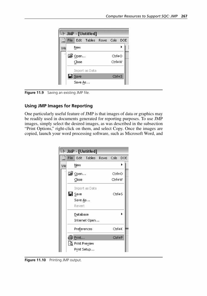
Computer Resources to Support SQC: JMP 267
Using JMP Images for Reporting
One particularly useful feature of JMP is that images of data or graphics may be readily used in documents generated for reporting purposes. To use JMP images, simply select the desired images, as was described in the subsection “Print Options,” right- click on them, and select Copy. Once the images are copied, launch your word processing software, such as Microsoft Word, and
Figure 11.9 Saving an existing JMP file.
Figure 11.10 Printing JMP output.
H1277 ch11.indd 267H1277 ch11.indd 267 3/8/07 12:39:50 PM3/8/07 12:39:50 PM

268 Chapter Eleven
then open your document and paste the images. This powerful feature elimi-nates the need for import/export functions.
11.2 The Shewhart XBar and R Control Chart
To create an XBar and R chart we begin by entering data into column 1 of a new data table. Once the data have been entered, we generate the chart by following the steps identified in Figure 11.11.
As can be seen in Figure 11.11, we first select Graph from the drop- down menu, then select Control Chart, and then XBar. A dialog box will be presented, as shown in Figure 11.12.
The dialog box in Figure 11.12 requires us to select a variable. The data table in this case contains only one variable, which is identified as “Column 1” in the Select Columns box, located in the upper left section of the dialog box. At this point, we would select the variable (click with the mouse) and assign it to the Process block, located in the upper center section of the dialog box, which indicates that a numeric variable is required.
Three additional points about the dialog box should be noted at this time. First, in an effort to anticipate the most frequently requested control chart, JMP automatically assumes we want to create an XBar and R chart. If any other type of variables control chart is desired, we must select the new
Figure 11.11 Generating an XBar and R chart.
H1277 ch11.indd 268H1277 ch11.indd 268 3/8/07 12:39:50 PM3/8/07 12:39:50 PM
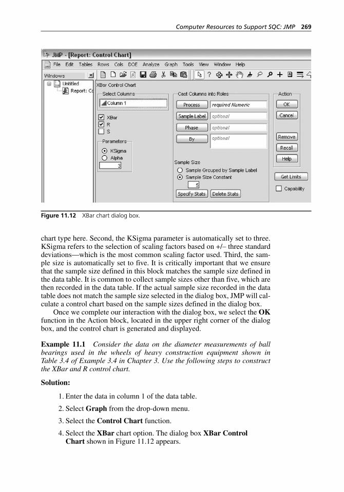
Computer Resources to Support SQC: JMP 269
chart type here. Second, the KSigma parameter is automatically set to three. KSigma refers to the selection of scaling factors based on +/– three standard deviations—which is the most common scaling factor used. Third, the sam-ple size is automatically set to five. It is critically important that we ensure that the sample size defined in this block matches the sample size defined in the data table. It is common to collect sample sizes other than five, which are then recorded in the data table. If the actual sample size recorded in the data table does not match the sample size selected in the dialog box, JMP will cal-culate a control chart based on the sample sizes defined in the dialog box.
Once we complete our interaction with the dialog box, we select the OK function in the Action block, located in the upper right corner of the dialog box, and the control chart is generated and displayed.
Example 11.1 Consider the data on the diameter measurements of ball bearings used in the wheels of heavy construction equipment shown in Table 3.4 of Example 3.4 in Chapter 3. Use the following steps to construct the XBar and R control chart.
Solution:
1. Enter the data in column 1 of the data table.
2. Select Graph from the drop- down menu.
3. Select the Control Chart function.
4. Select the XBar chart option. The dialog box XBar Control Chart shown in Figure 11.12 appears.
Figure 11.12 XBar chart dialog box.
H1277 ch11.indd 269H1277 ch11.indd 269 3/8/07 12:39:51 PM3/8/07 12:39:51 PM
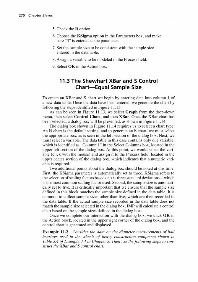
270 Chapter Eleven
5. Check the R option.
6. Choose the KSigma option in the Parameters box, and make sure “3” is entered as the parameter.
7. Set the sample size to be consistent with the sample size entered in the data table.
8. Assign a variable to be modeled in the Process field.
9. Select OK in the Action box.
11.3 The Shewhart XBar and S Control Chart—Equal Sample Size
To create an XBar and S chart we begin by entering data into column 1 of a new data table. Once the data have been entered, we generate the chart by following the steps identified in Figure 11.13.
As can be seen in Figure 11.13, we select Graph from the drop- down menu, then select Control Chart, and then XBar. Once the XBar chart has been selected, a dialog box will be presented, as shown in Figure 11.14.
The dialog box shown in Figure 11.14 requires us to select a chart type. An R chart is the default setting, and to generate an S chart, we must select the appropriate box, as is seen in the left section of the dialog box. Next, we must select a variable. The data table in this case contains only one variable, which is identified as “Column 1” in the Select Columns box, located in the upper left section of the dialog box. At this point, we would select the vari-able (click with the mouse) and assign it to the Process field, located in the upper center section of the dialog box, which indicates that a numeric vari-able is required.
Two additional points about the dialog box should be noted at this time. First, the KSigma parameter is automatically set to three. KSigma refers to the selection of scaling factors based on +/– three standard deviations—which is the most common scaling factor used. Second, the sample size is automati-cally set to five. It is critically important that we ensure that the sample size defined in this block matches the sample size defined in the data table. It is common to collect sample sizes other than five, which are then recorded in the data table. If the actual sample size recorded in the data table does not match the sample size selected in the dialog box, JMP will calculate a control chart based on the sample sizes defined in the dialog box.
Once we complete our interaction with the dialog box, we click OK in the Action block, located in the upper right corner of the dialog box, and the control chart is generated and displayed.
Example 11.2 Consider the data on the diameter measurements of ball bearings used in the wheels of heavy construction equipment shown in Table 3.4 of Example 3.4 in Chapter 3. Then use the following steps to con-struct the XBar and S control chart.
H1277 ch11.indd 270H1277 ch11.indd 270 3/8/07 12:39:51 PM3/8/07 12:39:51 PM
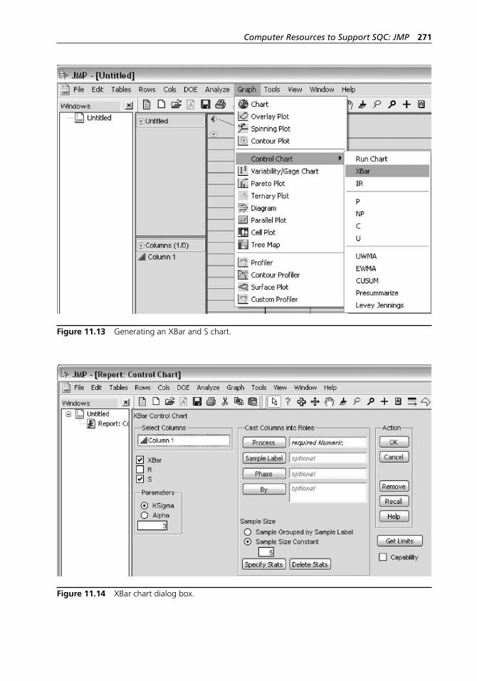
Computer Resources to Support SQC: JMP 271
Figure 11.13 Generating an XBar and S chart.
Figure 11.14 XBar chart dialog box.
H1277 ch11.indd 271H1277 ch11.indd 271 3/8/07 12:39:51 PM3/8/07 12:39:51 PM
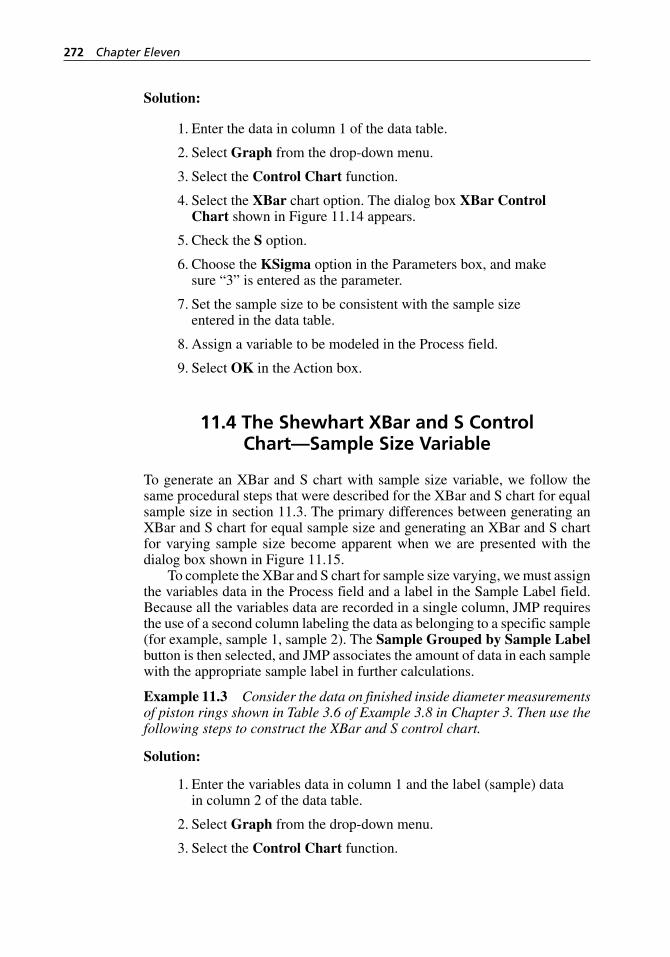
272 Chapter Eleven
Solution:
1. Enter the data in column 1 of the data table.
2. Select Graph from the drop- down menu.
3. Select the Control Chart function.
4. Select the XBar chart option. The dialog box XBar Control Chart shown in Figure 11.14 appears.
5. Check the S option.
6. Choose the KSigma option in the Parameters box, and make sure “3” is entered as the parameter.
7. Set the sample size to be consistent with the sample size entered in the data table.
8. Assign a variable to be modeled in the Process field.
9. Select OK in the Action box.
11.4 The Shewhart XBar and S Control Chart—Sample Size Variable
To generate an XBar and S chart with sample size variable, we follow the same procedural steps that were described for the XBar and S chart for equal sample size in section 11.3. The primary differences between generating an XBar and S chart for equal sample size and generating an XBar and S chart for varying sample size become apparent when we are presented with the dialog box shown in Figure 11.15.
To complete the XBar and S chart for sample size varying, we must assign the variables data in the Process field and a label in the Sample Label field. Because all the variables data are recorded in a single column, JMP requires the use of a second column labeling the data as belonging to a specific sample (for example, sample 1, sample 2). The Sample Grouped by Sample Label button is then selected, and JMP associates the amount of data in each sample with the appropriate sample label in further calculations.
Example 11.3 Consider the data on finished inside diameter measurements of piston rings shown in Table 3.6 of Example 3.8 in Chapter 3. Then use the following steps to construct the XBar and S control chart.
Solution:
1. Enter the variables data in column 1 and the label (sample) data in column 2 of the data table.
2. Select Graph from the drop- down menu.
3. Select the Control Chart function.
H1277 ch11.indd 272H1277 ch11.indd 272 3/8/07 12:39:52 PM3/8/07 12:39:52 PM
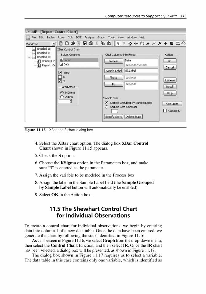
Computer Resources to Support SQC: JMP 273
4. Select the XBar chart option. The dialog box XBar Control Chart shown in Figure 11.15 appears.
5. Check the S option.
6. Choose the KSigma option in the Parameters box, and make sure “3” is entered as the parameter.
7. Assign the variable to be modeled in the Process box.
8. Assign the label in the Sample Label field (the Sample Grouped by Sample Label button will automatically be enabled).
9. Select OK in the Action box.
11.5 The Shewhart Control Chart for Individual Observations
To create a control chart for individual observations, we begin by entering data into column 1 of a new data table. Once the data have been entered, we generate the chart by following the steps identified in Figure 11.16.
As can be seen in Figure 11.16, we select Graph from the drop- down menu, then select the Control Chart function, and then select IR. Once the IR chart has been selected, a dialog box will be presented, as shown in Figure 11.17.
The dialog box shown in Figure 11.17 requires us to select a variable. The data table in this case contains only one variable, which is identified as
Figure 11.15 XBar and S chart dialog box.
H1277 ch11.indd 273H1277 ch11.indd 273 3/8/07 12:39:52 PM3/8/07 12:39:52 PM
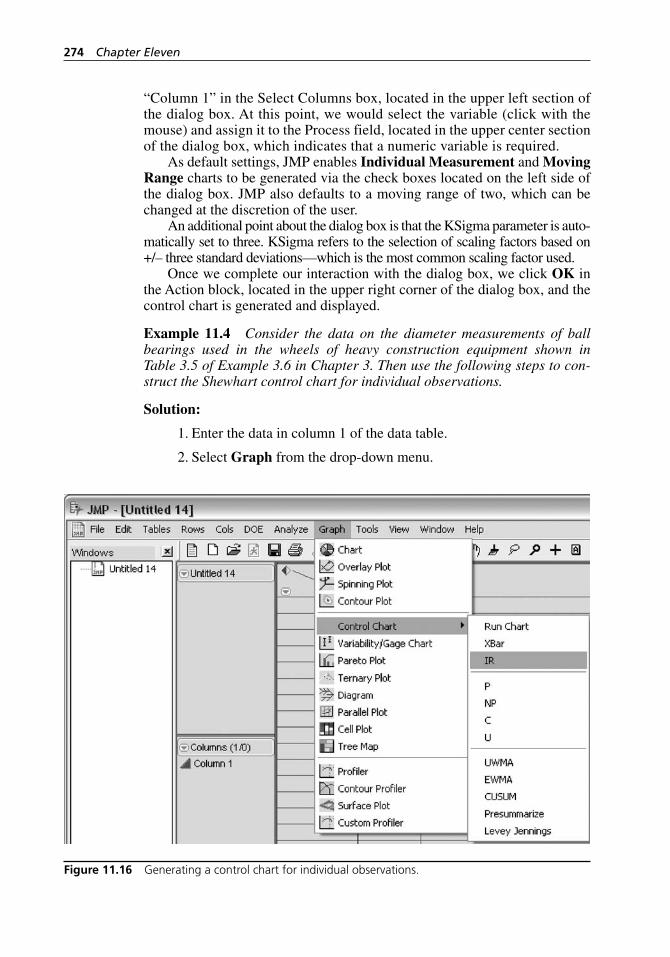
274 Chapter Eleven
“Column 1” in the Select Columns box, located in the upper left section of the dialog box. At this point, we would select the variable (click with the mouse) and assign it to the Process field, located in the upper center section of the dialog box, which indicates that a numeric variable is required.
As default settings, JMP enables Individual Measurement and Moving Range charts to be generated via the check boxes located on the left side of the dialog box. JMP also defaults to a moving range of two, which can be changed at the discretion of the user.
An additional point about the dialog box is that the KSigma parameter is auto-matically set to three. KSigma refers to the selection of scaling factors based on +/– three standard deviations—which is the most common scaling factor used.
Once we complete our interaction with the dialog box, we click OK in the Action block, located in the upper right corner of the dialog box, and the control chart is generated and displayed.
Example 11.4 Consider the data on the diameter measurements of ball bearings used in the wheels of heavy construction equipment shown in Table 3.5 of Example 3.6 in Chapter 3. Then use the following steps to con-struct the Shewhart control chart for individual observations.
Solution:
1. Enter the data in column 1 of the data table.
2. Select Graph from the drop- down menu.
Figure 11.16 Generating a control chart for individual observations.
H1277 ch11.indd 274H1277 ch11.indd 274 3/8/07 12:39:52 PM3/8/07 12:39:52 PM
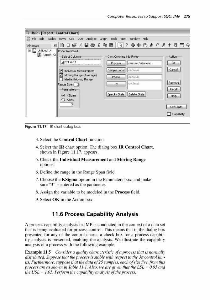
Computer Resources to Support SQC: JMP 275
3. Select the Control Chart function.
4. Select the IR chart option. The dialog box IR Control Chart, shown in Figure 11.17, appears.
5. Check the Individual Measurement and Moving Range options.
6. Define the range in the Range Span field.
7. Choose the KSigma option in the Parameters box, and make sure “3” is entered as the parameter.
8. Assign the variable to be modeled in the Process field.
9. Select OK in the Action box.
11.6 Process Capability Analysis
A process capability analysis in JMP is conducted in the context of a data set that is being evaluated for process control. This means that in the dialog box presented for any of the control charts, a check box for a process capabil-ity analysis is presented, enabling the analysis. We illustrate the capability analysis of a process with the following example.
Example 11.5 Consider a quality characteristic of a process that is normally distributed. Suppose that the process is stable with respect to the 3σ control lim-its. Furthermore, suppose that the data of 25 samples, each of size five, from this process are as shown in Table 11.1. Also, we are given that the LSL = 0.95 and the USL = 1.05. Perform the capability analysis of the process.
Figure 11.17 IR chart dialog box.
H1277 ch11.indd 275H1277 ch11.indd 275 3/8/07 12:39:53 PM3/8/07 12:39:53 PM
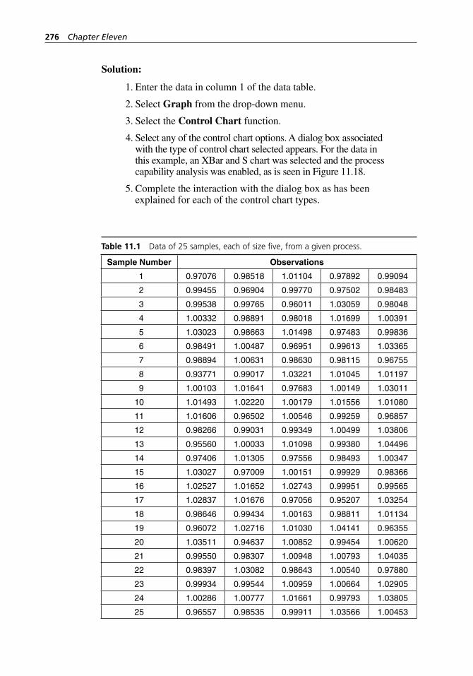
276 Chapter Eleven
Solution:
1. Enter the data in column 1 of the data table.
2. Select Graph from the drop- down menu.
3. Select the Control Chart function.
4. Select any of the control chart options. A dialog box associated with the type of control chart selected appears. For the data in this example, an XBar and S chart was selected and the process capability analysis was enabled, as is seen in Figure 11.18.
5. Complete the interaction with the dialog box as has been explained for each of the control chart types.
Table 11.1 Data of 25 samples, each of size five, from a given process.
Sample Number Observations
1 0.97076 0.98518 1.01104 0.97892 0.99094
2 0.99455 0.96904 0.99770 0.97502 0.98483
3 0.99538 0.99765 0.96011 1.03059 0.98048
4 1.00332 0.98891 0.98018 1.01699 1.00391
5 1.03023 0.98663 1.01498 0.97483 0.99836
6 0.98491 1.00487 0.96951 0.99613 1.03365
7 0.98894 1.00631 0.98630 0.98115 0.96755
8 0.93771 0.99017 1.03221 1.01045 1.01197
9 1.00103 1.01641 0.97683 1.00149 1.03011
10 1.01493 1.02220 1.00179 1.01556 1.01080
11 1.01606 0.96502 1.00546 0.99259 0.96857
12 0.98266 0.99031 0.99349 1.00499 1.03806
13 0.95560 1.00033 1.01098 0.99380 1.04496
14 0.97406 1.01305 0.97556 0.98493 1.00347
15 1.03027 0.97009 1.00151 0.99929 0.98366
16 1.02527 1.01652 1.02743 0.99951 0.99565
17 1.02837 1.01676 0.97056 0.95207 1.03254
18 0.98646 0.99434 1.00163 0.98811 1.01134
19 0.96072 1.02716 1.01030 1.04141 0.96355
20 1.03511 0.94637 1.00852 0.99454 1.00620
21 0.99550 0.98307 1.00948 1.00793 1.04035
22 0.98397 1.03082 0.98643 1.00540 0.97880
23 0.99934 0.99544 1.00959 1.00664 1.02905
24 1.00286 1.00777 1.01661 0.99793 1.03805
25 0.96557 0.98535 0.99911 1.03566 1.00453
H1277 ch11.indd 276H1277 ch11.indd 276 3/8/07 6:25:04 PM3/8/07 6:25:04 PM
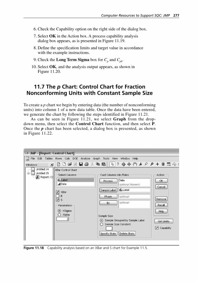
Computer Resources to Support SQC: JMP 277
6. Check the Capability option on the right side of the dialog box.
7. Select OK in the Action box. A process capability analysis dialog box appears, as is presented in Figure 11.19.
8. Define the specification limits and target value in accordance with the example instructions.
9. Check the Long Term Sigma box for Cp and Cpk.
10. Select OK, and the analysis output appears, as shown in Figure 11.20.
11.7 The p Chart: Control Chart for Fraction Nonconforming Units with Constant Sample Size
To create a p chart we begin by entering data (the number of nonconforming units) into column 1 of a new data table. Once the data have been entered, we generate the chart by following the steps identified in Figure 11.21.
As can be seen in Figure 11.21, we select Graph from the drop- down menu, then select the Control Chart function, and then select P. Once the p chart has been selected, a dialog box is presented, as shown in Figure 11.22.
Figure 11.18 Capability analysis based on an XBar and S chart for Example 11.5.
H1277 ch11.indd 277H1277 ch11.indd 277 3/8/07 12:39:53 PM3/8/07 12:39:53 PM
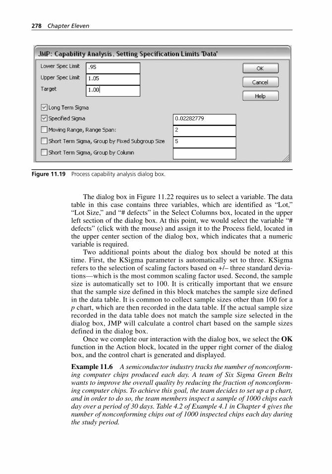
278 Chapter Eleven
The dialog box in Figure 11.22 requires us to select a variable. The data table in this case contains three variables, which are identified as “Lot,” “Lot Size,” and “# defects” in the Select Columns box, located in the upper left section of the dialog box. At this point, we would select the variable “# defects” (click with the mouse) and assign it to the Process field, located in the upper center section of the dialog box, which indicates that a numeric variable is required.
Two additional points about the dialog box should be noted at this time. First, the KSigma parameter is automatically set to three. KSigma refers to the selection of scaling factors based on +/– three standard devia-tions—which is the most common scaling factor used. Second, the sample size is automatically set to 100. It is critically important that we ensure that the sample size defined in this block matches the sample size defined in the data table. It is common to collect sample sizes other than 100 for a p chart, which are then recorded in the data table. If the actual sample size recorded in the data table does not match the sample size selected in the dialog box, JMP will calculate a control chart based on the sample sizes defined in the dialog box.
Once we complete our interaction with the dialog box, we select the OK function in the Action block, located in the upper right corner of the dialog box, and the control chart is generated and displayed.
Example 11.6 A semiconductor industry tracks the number of nonconform-ing computer chips produced each day. A team of Six Sigma Green Belts wants to improve the overall quality by reducing the fraction of nonconform-ing computer chips. To achieve this goal, the team decides to set up a p chart, and in order to do so, the team members inspect a sample of 1000 chips each day over a period of 30 days. Table 4.2 of Example 4.1 in Chapter 4 gives the number of nonconforming chips out of 1000 inspected chips each day during the study period.
Figure 11.19 Process capability analysis dialog box.
H1277 ch11.indd 278H1277 ch11.indd 278 3/8/07 12:39:54 PM3/8/07 12:39:54 PM
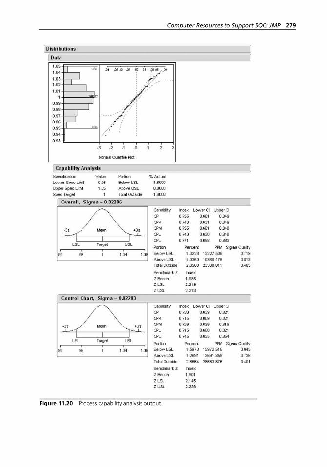
Computer Resources to Support SQC: JMP 279
Figure 11.20 Process capability analysis output.
H1277 ch11.indd 279H1277 ch11.indd 279 3/8/07 12:39:54 PM3/8/07 12:39:54 PM
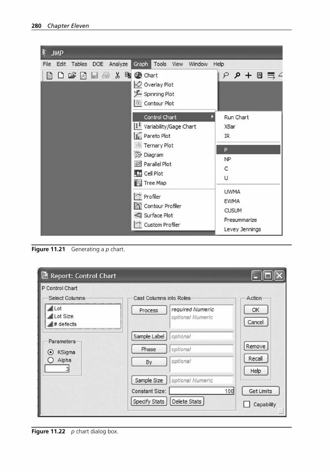
280 Chapter Eleven
Figure 11.21 Generating a p chart.
Figure 11.22 p chart dialog box.
H1277 ch11.indd 280H1277 ch11.indd 280 3/8/07 12:39:55 PM3/8/07 12:39:55 PM
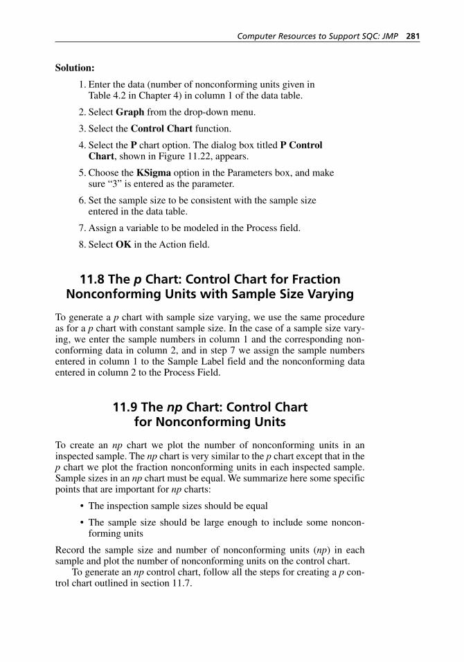
Computer Resources to Support SQC: JMP 281
Solution:
1. Enter the data (number of nonconforming units given in Table 4.2 in Chapter 4) in column 1 of the data table.
2. Select Graph from the drop- down menu.
3. Select the Control Chart function.
4. Select the P chart option. The dialog box titled P Control Chart, shown in Figure 11.22, appears.
5. Choose the KSigma option in the Parameters box, and make sure “3” is entered as the parameter.
6. Set the sample size to be consistent with the sample size entered in the data table.
7. Assign a variable to be modeled in the Process field.
8. Select OK in the Action field.
11.8 The p Chart: Control Chart for Fraction Nonconforming Units with Sample Size Varying
To generate a p chart with sample size varying, we use the same procedure as for a p chart with constant sample size. In the case of a sample size vary-ing, we enter the sample numbers in column 1 and the corresponding non-conforming data in column 2, and in step 7 we assign the sample numbers entered in column 1 to the Sample Label field and the nonconforming data entered in column 2 to the Process Field.
11.9 The np Chart: Control Chart for Nonconforming Units
To create an np chart we plot the number of nonconforming units in an inspected sample. The np chart is very similar to the p chart except that in the p chart we plot the fraction nonconforming units in each inspected sample. Sample sizes in an np chart must be equal. We summarize here some specific points that are important for np charts:
The inspection sample sizes should be equal
The sample size should be large enough to include some noncon-forming units
Record the sample size and number of nonconforming units (np) in each sample and plot the number of nonconforming units on the control chart.
To generate an np control chart, follow all the steps for creating a p con-trol chart outlined in section 11.7.
•
•
H1277 ch11.indd 281H1277 ch11.indd 281 3/8/07 12:39:56 PM3/8/07 12:39:56 PM
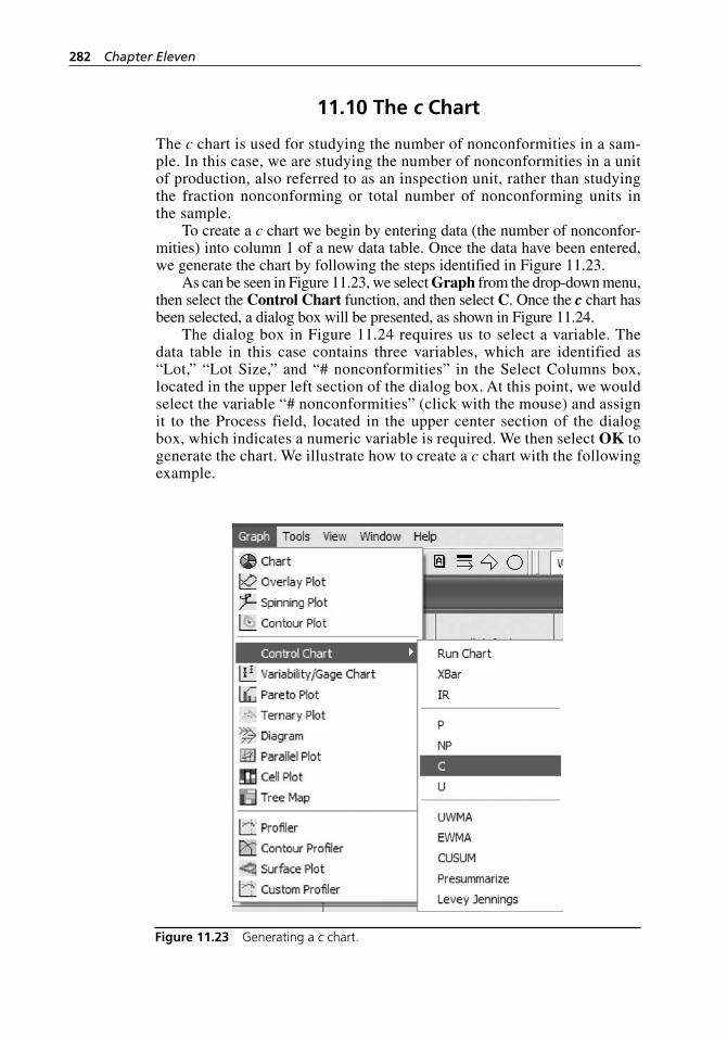
282 Chapter Eleven
11.10 The c Chart
The c chart is used for studying the number of nonconformities in a sam-ple. In this case, we are studying the number of nonconformities in a unit of production, also referred to as an inspection unit, rather than studying the fraction nonconforming or total number of nonconforming units in the sample.
To create a c chart we begin by entering data (the number of nonconfor-mities) into column 1 of a new data table. Once the data have been entered, we generate the chart by following the steps identified in Figure 11.23.
As can be seen in Figure 11.23, we select Graph from the drop- down menu, then select the Control Chart function, and then select C. Once the c chart has been selected, a dialog box will be presented, as shown in Figure 11.24.
The dialog box in Figure 11.24 requires us to select a variable. The data table in this case contains three variables, which are identified as “Lot,” “Lot Size,” and “# nonconformities” in the Select Columns box, located in the upper left section of the dialog box. At this point, we would select the variable “# nonconformities” (click with the mouse) and assign it to the Process field, located in the upper center section of the dialog box, which indicates a numeric variable is required. We then select OK to generate the chart. We illustrate how to create a c chart with the following example.
Figure 11.23 Generating a c chart.
H1277 ch11.indd 282H1277 ch11.indd 282 3/8/07 12:39:56 PM3/8/07 12:39:56 PM
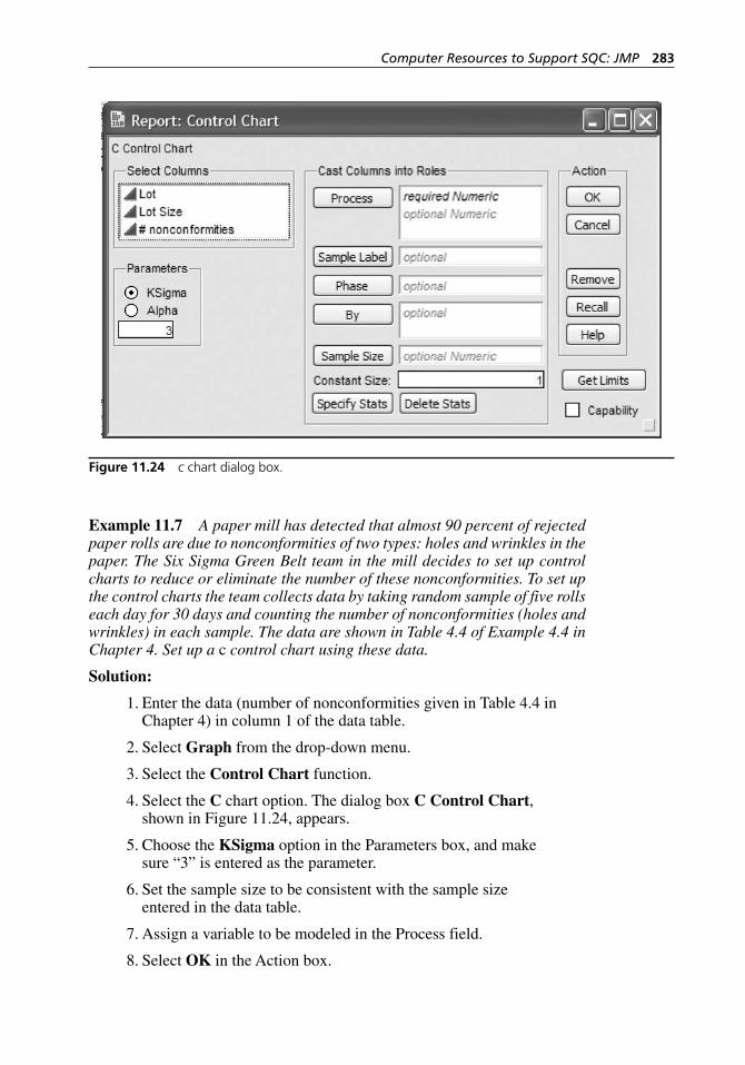
Computer Resources to Support SQC: JMP 283
Example 11.7 A paper mill has detected that almost 90 percent of rejected paper rolls are due to nonconformities of two types: holes and wrinkles in the paper. The Six Sigma Green Belt team in the mill decides to set up control charts to reduce or eliminate the number of these nonconformities. To set up the control charts the team collects data by taking random sample of five rolls each day for 30 days and counting the number of nonconformities (holes and wrinkles) in each sample. The data are shown in Table 4.4 of Example 4.4 in Chapter 4. Set up a c control chart using these data.
Solution:
1. Enter the data (number of nonconformities given in Table 4.4 in Chapter 4) in column 1 of the data table.
2. Select Graph from the drop- down menu.
3. Select the Control Chart function.
4. Select the C chart option. The dialog box C Control Chart, shown in Figure 11.24, appears.
5. Choose the KSigma option in the Parameters box, and make sure “3” is entered as the parameter.
6. Set the sample size to be consistent with the sample size entered in the data table.
7. Assign a variable to be modeled in the Process field.
8. Select OK in the Action box.
Figure 11.24 c chart dialog box.
H1277 ch11.indd 283H1277 ch11.indd 283 3/8/07 12:39:56 PM3/8/07 12:39:56 PM
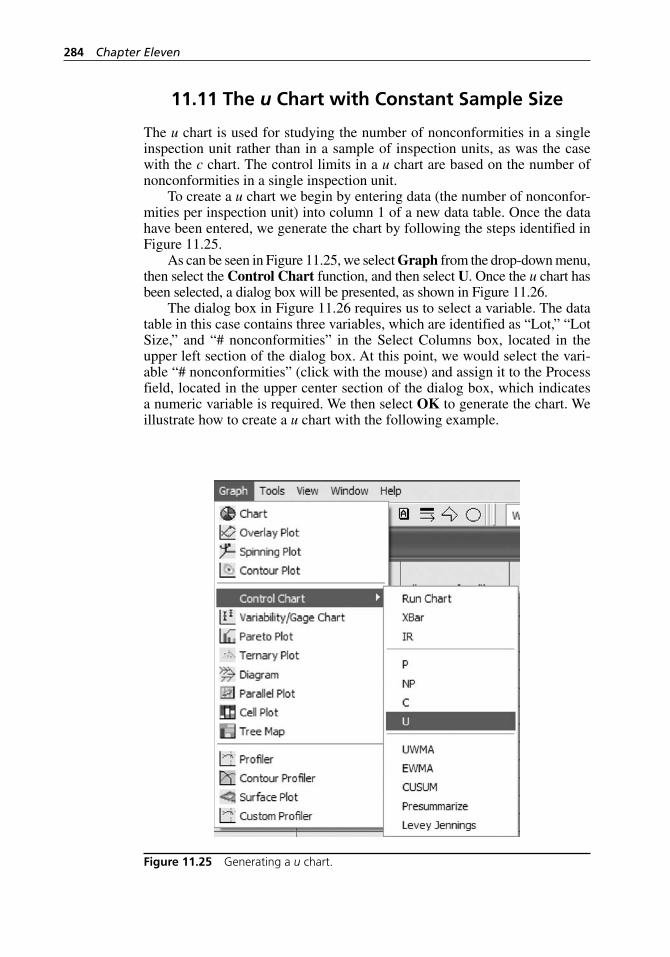
284 Chapter Eleven
11.11 The u Chart with Constant Sample Size
The u chart is used for studying the number of nonconformities in a single inspection unit rather than in a sample of inspection units, as was the case with the c chart. The control limits in a u chart are based on the number of nonconformities in a single inspection unit.
To create a u chart we begin by entering data (the number of nonconfor-mities per inspection unit) into column 1 of a new data table. Once the data have been entered, we generate the chart by following the steps identified in Figure 11.25.
As can be seen in Figure 11.25, we select Graph from the drop- down menu, then select the Control Chart function, and then select U. Once the u chart has been selected, a dialog box will be presented, as shown in Figure 11.26.
The dialog box in Figure 11.26 requires us to select a variable. The data table in this case contains three variables, which are identified as “Lot,” “Lot Size,” and “# nonconformities” in the Select Columns box, located in the upper left section of the dialog box. At this point, we would select the vari-able “# nonconformities” (click with the mouse) and assign it to the Process field, located in the upper center section of the dialog box, which indicates a numeric variable is required. We then select OK to generate the chart. We illustrate how to create a u chart with the following example.
Figure 11.25 Generating a u chart.
H1277 ch11.indd 284H1277 ch11.indd 284 3/8/07 12:39:57 PM3/8/07 12:39:57 PM
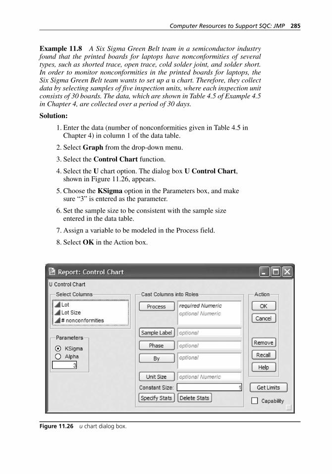
Computer Resources to Support SQC: JMP 285
Example 11.8 A Six Sigma Green Belt team in a semiconductor industry found that the printed boards for laptops have nonconformities of several types, such as shorted trace, open trace, cold solder joint, and solder short. In order to monitor nonconformities in the printed boards for laptops, the Six Sigma Green Belt team wants to set up a u chart. Therefore, they collect data by selecting samples of five inspection units, where each inspection unit consists of 30 boards. The data, which are shown in Table 4.5 of Example 4.5 in Chapter 4, are collected over a period of 30 days.
Solution:
1. Enter the data (number of nonconformities given in Table 4.5 in Chapter 4) in column 1 of the data table.
2. Select Graph from the drop- down menu.
3. Select the Control Chart function.
4. Select the U chart option. The dialog box U Control Chart, shown in Figure 11.26, appears.
5. Choose the KSigma option in the Parameters box, and make sure “3” is entered as the parameter.
6. Set the sample size to be consistent with the sample size entered in the data table.
7. Assign a variable to be modeled in the Process field.
8. Select OK in the Action box.
Figure 11.26 u chart dialog box.
H1277 ch11.indd 285H1277 ch11.indd 285 3/8/07 12:39:57 PM3/8/07 12:39:57 PM
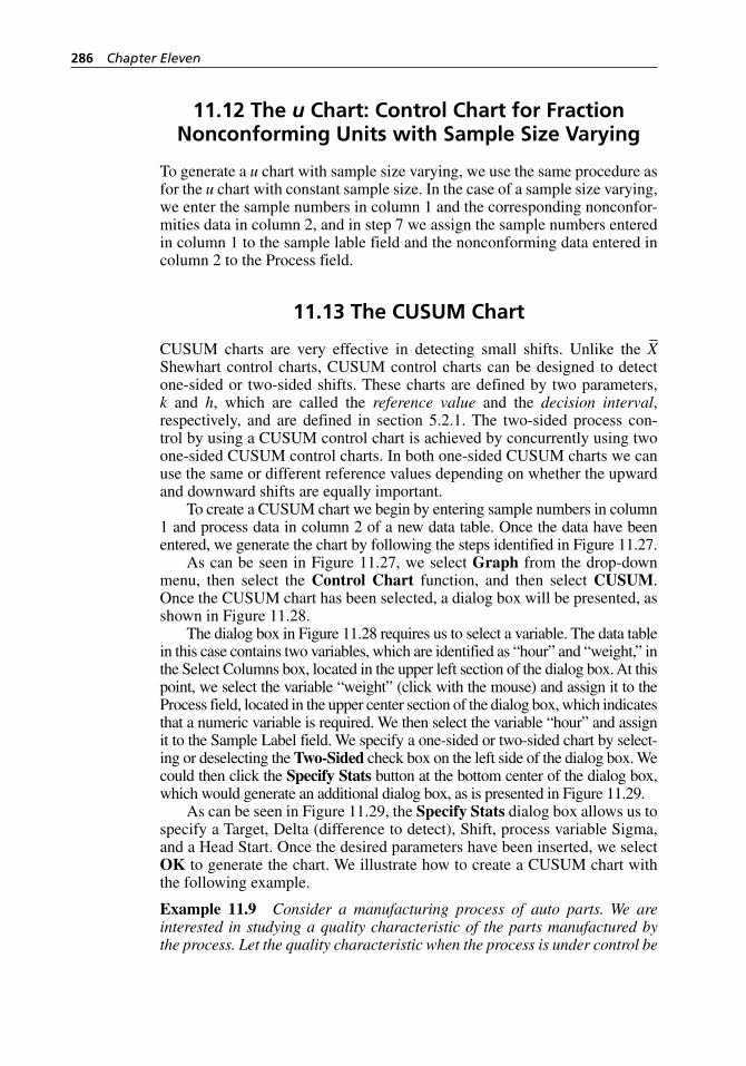
286 Chapter Eleven
11.12 The u Chart: Control Chart for Fraction Nonconforming Units with Sample Size Varying
To generate a u chart with sample size varying, we use the same procedure as for the u chart with constant sample size. In the case of a sample size varying, we enter the sample numbers in column 1 and the corresponding nonconfor-mities data in column 2, and in step 7 we assign the sample numbers entered in column 1 to the sample lable field and the nonconforming data entered in column 2 to the Process field.
11.13 The CUSUM Chart
CUSUM charts are very effective in detecting small shifts. Unlike the X–
Shewhart control charts, CUSUM control charts can be designed to detect one- sided or two- sided shifts. These charts are defined by two parameters, k and h, which are called the reference value and the decision interval, respectively, and are defined in section 5.2.1. The two- sided process con-trol by using a CUSUM control chart is achieved by concurrently using two one- sided CUSUM control charts. In both one- sided CUSUM charts we can use the same or different reference values depending on whether the upward and downward shifts are equally important.
To create a CUSUM chart we begin by entering sample numbers in column 1 and process data in column 2 of a new data table. Once the data have been entered, we generate the chart by following the steps identified in Figure 11.27.
As can be seen in Figure 11.27, we select Graph from the drop- down menu, then select the Control Chart function, and then select CUSUM. Once the CUSUM chart has been selected, a dialog box will be presented, as shown in Figure 11.28.
The dialog box in Figure 11.28 requires us to select a variable. The data table in this case contains two variables, which are identified as “hour” and “weight,” in the Select Columns box, located in the upper left section of the dialog box. At this point, we select the variable “weight” (click with the mouse) and assign it to the Process field, located in the upper center section of the dialog box, which indicates that a numeric variable is required. We then select the variable “hour” and assign it to the Sample Label field. We specify a one- sided or two- sided chart by select-ing or deselecting the Two-Sided check box on the left side of the dialog box. We could then click the Specify Stats button at the bottom center of the dialog box, which would generate an additional dialog box, as is presented in Figure 11.29.
As can be seen in Figure 11.29, the Specify Stats dialog box allows us to specify a Target, Delta (difference to detect), Shift, process variable Sigma, and a Head Start. Once the desired parameters have been inserted, we select OK to generate the chart. We illustrate how to create a CUSUM chart with the following example.
Example 11.9 Consider a manufacturing process of auto parts. We are interested in studying a quality characteristic of the parts manufactured by the process. Let the quality characteristic when the process is under control be
H1277 ch11.indd 286H1277 ch11.indd 286 3/8/07 12:39:57 PM3/8/07 12:39:57 PM
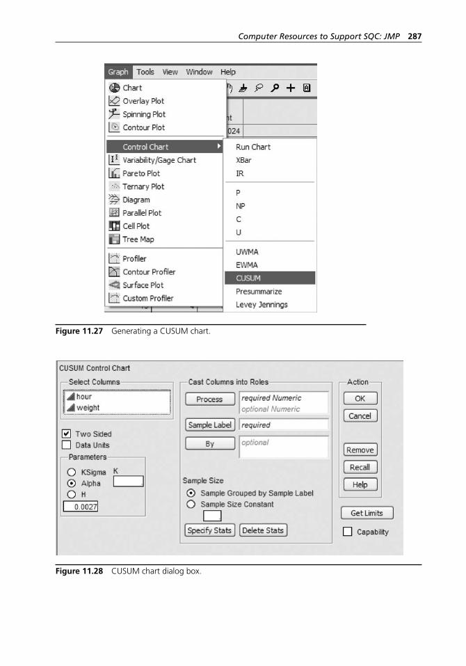
Computer Resources to Support SQC: JMP 287
Figure 11.27 Generating a CUSUM chart.
Figure 11.28 CUSUM chart dialog box.
H1277 ch11.indd 287H1277 ch11.indd 287 3/8/07 12:39:58 PM3/8/07 12:39:58 PM
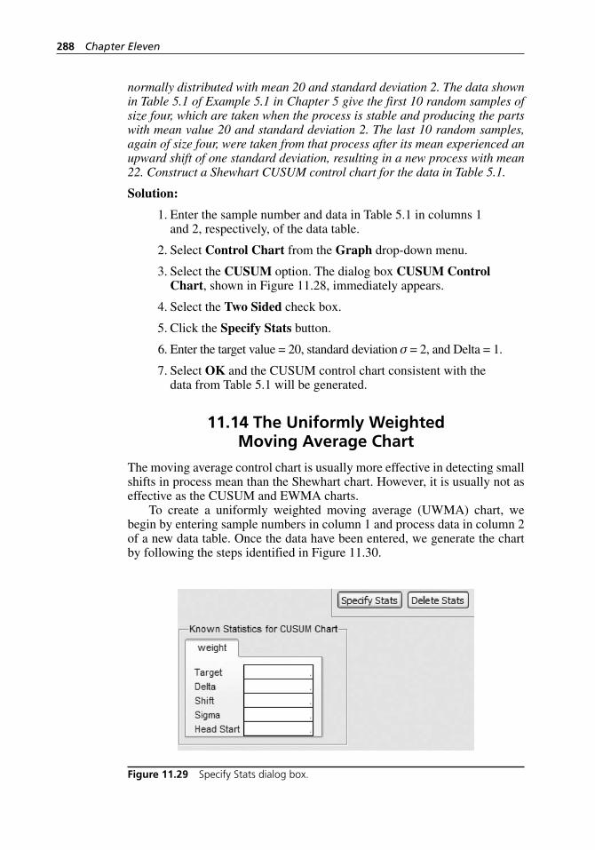
288 Chapter Eleven
normally distributed with mean 20 and standard deviation 2. The data shown in Table 5.1 of Example 5.1 in Chapter 5 give the first 10 random samples of size four, which are taken when the process is stable and producing the parts with mean value 20 and standard deviation 2. The last 10 random samples, again of size four, were taken from that process after its mean experienced an upward shift of one standard deviation, resulting in a new process with mean 22. Construct a Shewhart CUSUM control chart for the data in Table 5.1.
Solution:
1. Enter the sample number and data in Table 5.1 in columns 1 and 2, respectively, of the data table.
2. Select Control Chart from the Graph drop- down menu.
3. Select the CUSUM option. The dialog box CUSUM Control Chart, shown in Figure 11.28, immediately appears.
4. Select the Two Sided check box.
5. Click the Specify Stats button.
6. Enter the target value = 20, standard deviation σ = 2, and Delta = 1.
7. Select OK and the CUSUM control chart consistent with the data from Table 5.1 will be generated.
11.14 The Uniformly Weighted Moving Average Chart
The moving average control chart is usually more effective in detecting small shifts in process mean than the Shewhart chart. However, it is usually not as effective as the CUSUM and EWMA charts.
To create a uniformly weighted moving average (UWMA) chart, we begin by entering sample numbers in column 1 and process data in column 2 of a new data table. Once the data have been entered, we generate the chart by following the steps identified in Figure 11.30.
Figure 11.29 Specify Stats dialog box.
H1277 ch11.indd 288H1277 ch11.indd 288 3/8/07 12:39:58 PM3/8/07 12:39:58 PM
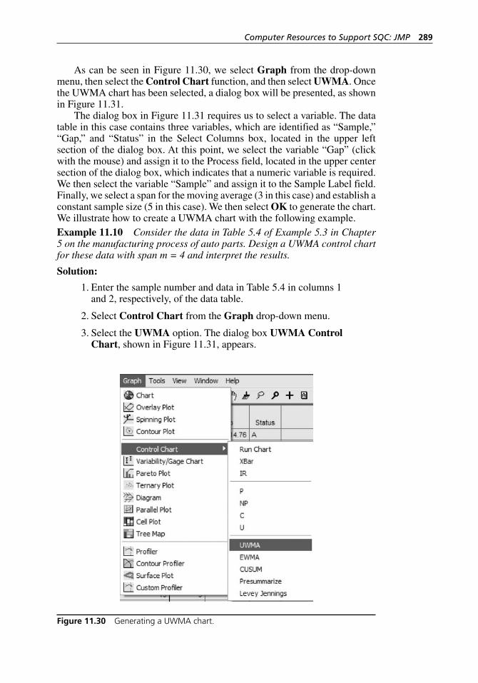
Computer Resources to Support SQC: JMP 289
As can be seen in Figure 11.30, we select Graph from the drop- down menu, then select the Control Chart function, and then select UWMA. Once the UWMA chart has been selected, a dialog box will be presented, as shown in Figure 11.31.
The dialog box in Figure 11.31 requires us to select a variable. The data table in this case contains three variables, which are identified as “Sample,” “Gap,” and “Status” in the Select Columns box, located in the upper left section of the dialog box. At this point, we select the variable “Gap” (click with the mouse) and assign it to the Process field, located in the upper center section of the dialog box, which indicates that a numeric variable is required. We then select the variable “Sample” and assign it to the Sample Label field. Finally, we select a span for the moving average (3 in this case) and establish a constant sample size (5 in this case). We then select OK to generate the chart. We illustrate how to create a UWMA chart with the following example.Example 11.10 Consider the data in Table 5.4 of Example 5.3 in Chapter 5 on the manufacturing process of auto parts. Design a UWMA control chart for these data with span m = 4 and interpret the results.
Solution:
1. Enter the sample number and data in Table 5.4 in columns 1 and 2, respectively, of the data table.
2. Select Control Chart from the Graph drop- down menu.
3. Select the UWMA option. The dialog box UWMA Control Chart, shown in Figure 11.31, appears.
Figure 11.30 Generating a UWMA chart.
H1277 ch11.indd 289H1277 ch11.indd 289 3/8/07 12:39:58 PM3/8/07 12:39:58 PM
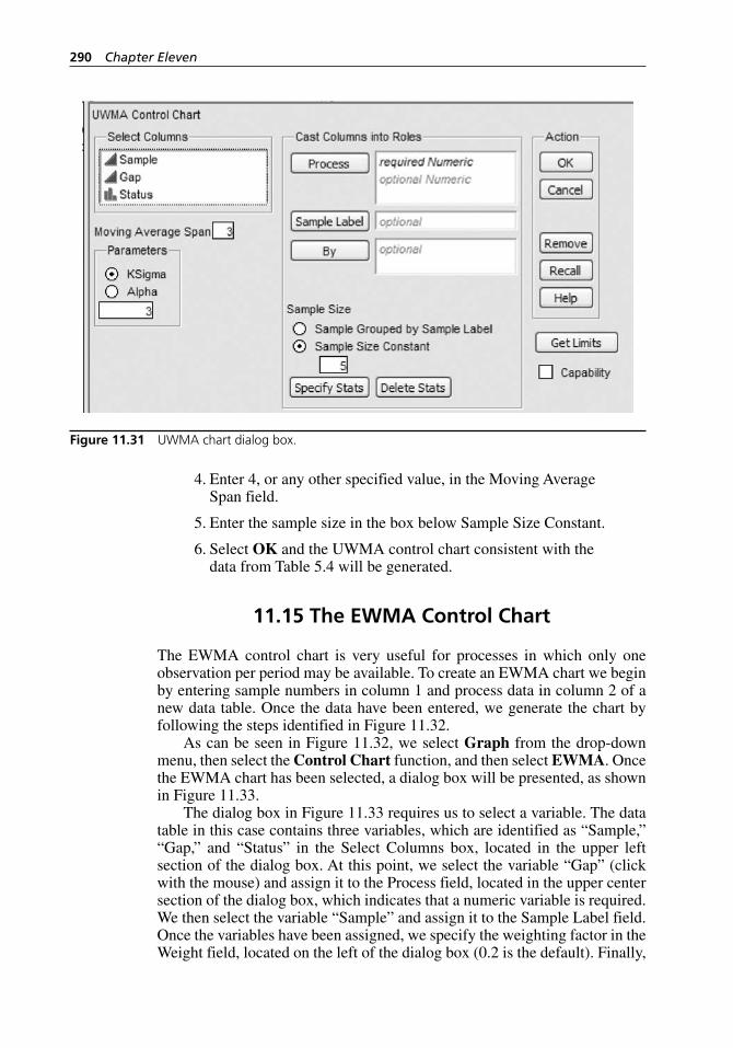
290 Chapter Eleven
4. Enter 4, or any other specified value, in the Moving Average Span field.
5. Enter the sample size in the box below Sample Size Constant.
6. Select OK and the UWMA control chart consistent with the data from Table 5.4 will be generated.
11.15 The EWMA Control Chart
The EWMA control chart is very useful for processes in which only one observation per period may be available. To create an EWMA chart we begin by entering sample numbers in column 1 and process data in column 2 of a new data table. Once the data have been entered, we generate the chart by following the steps identified in Figure 11.32.
As can be seen in Figure 11.32, we select Graph from the drop- down menu, then select the Control Chart function, and then select EWMA. Once the EWMA chart has been selected, a dialog box will be presented, as shown in Figure 11.33.
The dialog box in Figure 11.33 requires us to select a variable. The data table in this case contains three variables, which are identified as “Sample,” “Gap,” and “Status” in the Select Columns box, located in the upper left section of the dialog box. At this point, we select the variable “Gap” (click with the mouse) and assign it to the Process field, located in the upper center section of the dialog box, which indicates that a numeric variable is required. We then select the variable “Sample” and assign it to the Sample Label field. Once the variables have been assigned, we specify the weighting factor in the Weight field, located on the left of the dialog box (0.2 is the default). Finally,
Figure 11.31 UWMA chart dialog box.
H1277 ch11.indd 290H1277 ch11.indd 290 3/8/07 12:39:59 PM3/8/07 12:39:59 PM
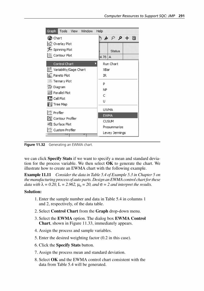
Computer Resources to Support SQC: JMP 291
we can click Specify Stats if we want to specify a mean and standard devia-tion for the process variable. We then select OK to generate the chart. We illustrate how to create an EWMA chart with the following example.
Example 11.11 Consider the data in Table 5.4 of Example 5.3 in Chapter 5 on the manufacturing process of auto parts. Design an EWMA control chart for these data with λ = 0.20, L = 2.962, µ0 = 20, and σ = 2 and interpret the results.
Solution:
1. Enter the sample number and data in Table 5.4 in columns 1 and 2, respectively, of the data table.
2. Select Control Chart from the Graph drop- down menu.
3. Select the EWMA option. The dialog box EWMA Control Chart, shown in Figure 11.33, immediately appears.
4. Assign the process and sample variables.
5. Enter the desired weighting factor (0.2 in this case).
6. Click the Specify Stats button.
7. Assign the process mean and standard deviation.
8. Select OK and the EWMA control chart consistent with the data from Table 5.4 will be generated.
Figure 11.32 Generating an EWMA chart.
H1277 ch11.indd 291H1277 ch11.indd 291 3/8/07 12:39:59 PM3/8/07 12:39:59 PM
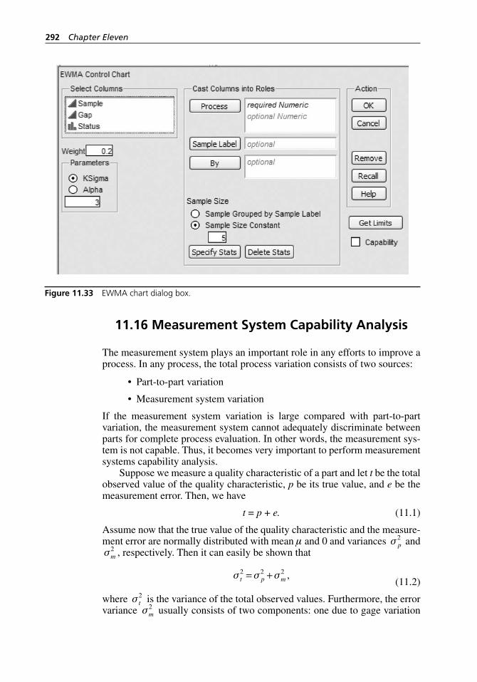
292 Chapter Eleven
11.16 Measurement System Capability Analysis
The measurement system plays an important role in any efforts to improve a process. In any process, the total process variation consists of two sources:
Part-to-part variation
Measurement system variation
If the measurement system variation is large compared with part- to-part variation, the measurement system cannot adequately discriminate between parts for complete process evaluation. In other words, the measurement sys-tem is not capable. Thus, it becomes very important to perform measurement systems capability analysis.
Suppose we measure a quality characteristic of a part and let t be the total observed value of the quality characteristic, p be its true value, and e be the measurement error. Then, we have
t = p + e. (11.1)
Assume now that the true value of the quality characteristic and the measure-ment error are normally distributed with mean µ and 0 and variances σ p
2 and σm
2 , respectively. Then it can easily be shown that
σ σ σt p m
2 2 2= + , (11.2)
where σ t2 is the variance of the total observed values. Furthermore, the error
variance σm2 usually consists of two components: one due to gage variation
•
•
Figure 11.33 EWMA chart dialog box.
H1277 ch11.indd 292H1277 ch11.indd 292 3/8/07 12:40:00 PM3/8/07 12:40:00 PM
Computer Resources to Support SQC: JMP 293
(repeatability) and the other due to operator variation (reproducibility). The purpose of measurement system capability analysis is to separate these com-ponents and analyze them. In other words, we have
σ σ σmeasurement error reproducibilty repea
2 2= + ttability2 .
To study these components, we usually use the ANOVA technique, which is also known as Gage R&R study. When using the ANOVA technique, we commonly deal with two types of situations: (1) when each operator mea-sures the same specimens of a part, and (2) when each operator measures dif-ferent specimens of a part. The designs used in these situations are known as crossed and nested designs, respectively. The following section discusses the Gage R&R study using JMP and crossed designs. We do not discuss nested designs here, as they are beyond the scope of this book.
11.16.1 Measurement System Capability Analysis (Using Crossed Designs)
A manufacturer of tubes used in automotive applications has installed a new measuring gage. The Six Sigma Green Belt team is interested in determin-ing how well the new gage measures the inside diameter of the tube. In other words, the team is interested in performing the measurement system capabil-ity analysis. We discuss the measurement system capability analysis with the following example.
Example 11.12 A manufacturer of bolts (parts) used in automotive applications has installed a new measuring gage. In order to perform the MSA on the new gage, the quality manager randomly selects three Six Sigma Green Belt operators from the department of quality control, who decide to take a random sample of 10 bolts. Each operator takes three measurements on each bolt, which is selected randomly. The data obtained are shown in Table 11.2.
Estimate the repeatability and reproducibility of the measurement system.
Estimate how much of the total process variation is due to the mea-surement system.
If the tube diameter specifications are 70 ± 10, what can we say about the discrimination power of the measurement system? In other words, is the measurement system capable of discriminating between different parts?
Solution: We have already discussed this example earlier, in Chapter 7. Here we discuss step by step how to set up JMP to find the solution to this or any other similar problem.
•
•
•
H1277 ch11.indd 293H1277 ch11.indd 293 3/8/07 12:40:00 PM3/8/07 12:40:00 PM
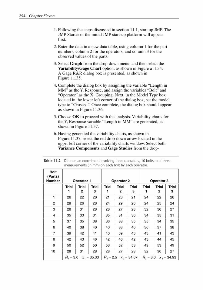
294 Chapter Eleven
1. Following the steps discussed in section 11.1, start up JMP. The JMP Starter or the initial JMP start- up platform will appear first.
2. Enter the data in a new data table, using column 1 for the part numbers, column 2 for the operators, and column 3 for the observed values of the parts.
3. Select Graph from the drop- down menu, and then select the Variability/Gage Chart option, as shown in Figure a11.34. A Gage R&R dialog box is presented, as shown in Figure 11.35.
4. Complete the dialog box by assigning the variable “Length in MM” as the Y, Response, and assign the variables “Bolt” and “Operator” as the X, Grouping. Next, in the Model Type box located in the lower left corner of the dialog box, set the model type to “Crossed.” Once complete, the dialog box should appear as shown in Figure 11.36.
5. Choose OK to proceed with the analysis. Variability charts for the Y, Response variable “Length in MM” are generated, as shown in Figure 11.37.
6. Having generated the variability charts, as shown in Figure 11.37, select the red drop- down arrow located in the upper left corner of the variability charts window. Select both Variance Components and Gage Studies from the drop-
Table 11.2 Data on an experiment involving three operators, 10 bolts, and three measurements (in mm) on each bolt by each operator.
Bolt (Parts)
Number Operator 1 Operator 2 Operator 3
Trial 1
Trial 2
Trial 3
Trial 1
Trial 2
Trial 3
Trial 1
Trial 2
Trial 3
1 26 22 26 21 23 21 24 22 26
2 28 26 28 24 29 26 24 25 24
3 28 31 28 28 27 28 32 30 27
4 35 33 31 35 31 30 34 35 31
5 37 35 38 36 38 35 35 34 35
6 40 38 40 40 38 40 36 37 38
7 39 42 41 40 39 43 43 41 43
8 42 43 46 42 46 42 43 44 45
9 50 52 50 53 52 53 49 53 49
10 28 31 28 28 27 28 32 30 27
R–
1 = 3.0 x–1 = 35.33 R–
2 = 2.5 x–2 = 34.67 R–
3 = 3.0 x–3 = 34.93
H1277 ch11.indd 294H1277 ch11.indd 294 3/8/07 6:25:14 PM3/8/07 6:25:14 PM
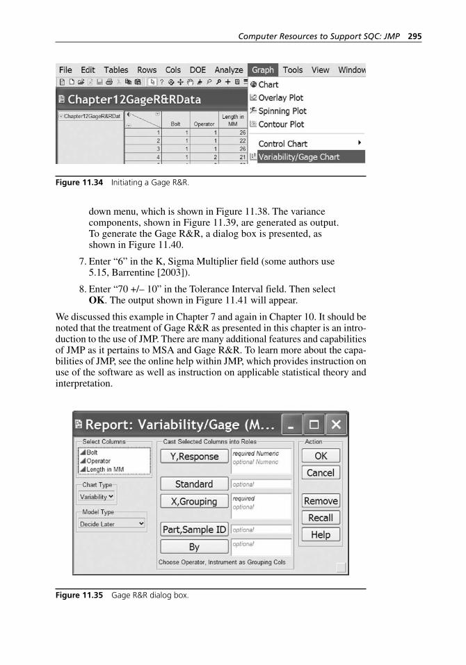
Computer Resources to Support SQC: JMP 295
down menu, which is shown in Figure 11.38. The variance components, shown in Figure 11.39, are generated as output. To generate the Gage R&R, a dialog box is presented, as shown in Figure 11.40.
7. Enter “6” in the K, Sigma Multiplier field (some authors use 5.15, Barrentine [2003]).
8. Enter “70 +/– 10” in the Tolerance Interval field. Then select OK. The output shown in Figure 11.41 will appear.
We discussed this example in Chapter 7 and again in Chapter 10. It should be noted that the treatment of Gage R&R as presented in this chapter is an intro-duction to the use of JMP. There are many additional features and capabilities of JMP as it pertains to MSA and Gage R&R. To learn more about the capa-bilities of JMP, see the online help within JMP, which provides instruction on use of the software as well as instruction on applicable statistical theory and interpretation.
Figure 11.34 Initiating a Gage R&R.
Figure 11.35 Gage R&R dialog box.
H1277 ch11.indd 295H1277 ch11.indd 295 3/8/07 12:40:00 PM3/8/07 12:40:00 PM
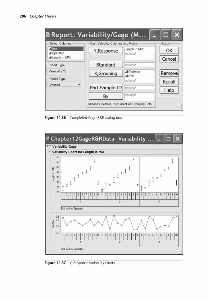
296 Chapter Eleven
Figure 11.36 Completed Gage R&R dialog box.
Figure 11.37 Y, Response variability charts.
H1277 ch11.indd 296H1277 ch11.indd 296 3/8/07 12:40:01 PM3/8/07 12:40:01 PM
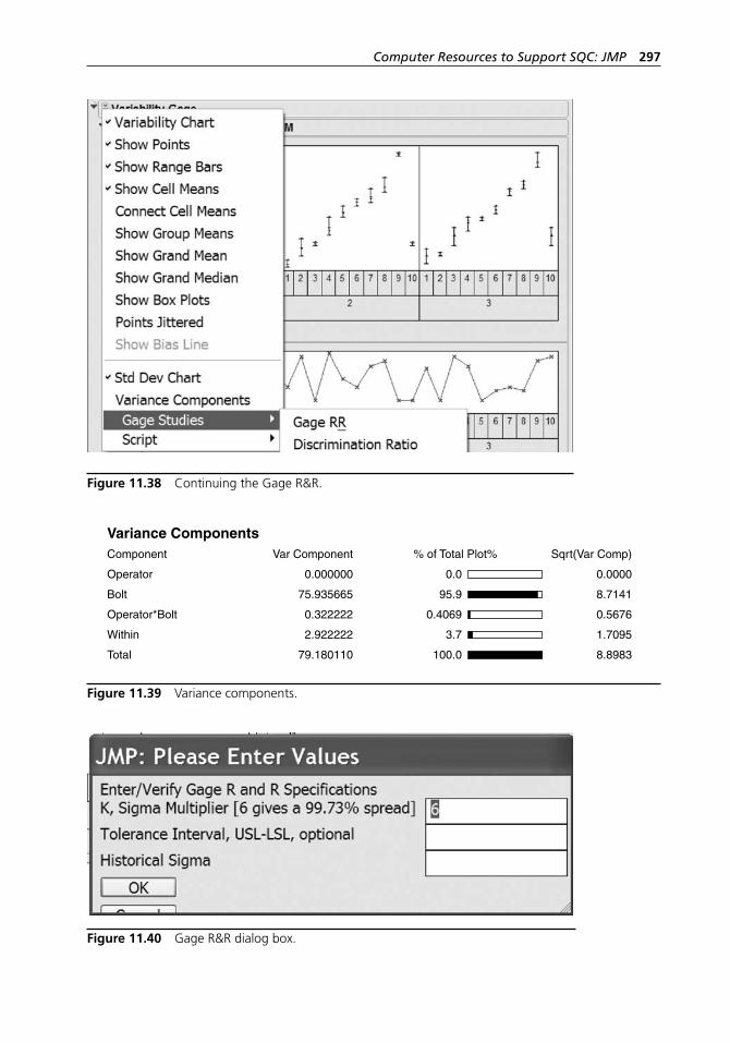
Computer Resources to Support SQC: JMP 297
Figure 11.38 Continuing the Gage R&R.
Variance ComponentsComponent Var Component % of Total Plot% Sqrt(Var Comp)
Operator 0.000000 0.0 0.0000
Bolt 75.935665 95.9 8.7141
Operator*Bolt 0.322222 0.4069 0.5676
Within 2.922222 3.7 1.7095
Total 79.180110 100.0 8.8983
Figure 11.39 Variance components.
Figure 11.40 Gage R&R dialog box.
H1277 ch11.indd 297H1277 ch11.indd 297 3/8/07 12:40:02 PM3/8/07 12:40:02 PM
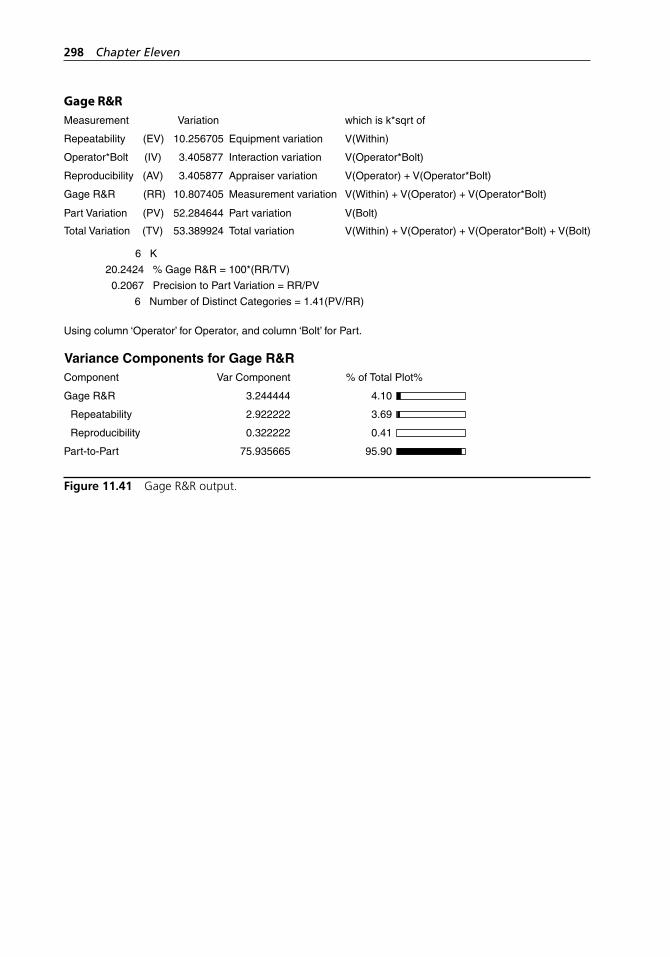
298 Chapter Eleven
Variance Components for Gage R&RComponent Var Component % of Total Plot%
Gage R&R 3.244444 4.10
Repeatability 2.922222 3.69
Reproducibility 0.322222 0.41
Part-to-Part 75.935665 95.90
Gage R&R
Gage R&R
Measurement
Repeatability
Operator*Bolt
Reproducibility
Part Variation
Total Variation
(EV)
(IV)
(AV)
(RR)
(PV)
(TV)
Variation
10.256705
3.405877
3.405877
10.807405
52.284644
53.389924
Equipment variation
Interaction variation
Appraiser variation
Measurement variation
Part variation
Total variation
which is k*sqrt of
V(Within)
V(Operator*Bolt)
V(Operator) + V(Operator*Bolt)
V(Within) + V(Operator) + V(Operator*Bolt)
V(Bolt)
V(Within) + V(Operator) + V(Operator*Bolt) + V(Bolt)
6 K
20.2424 % Gage R&R = 100*(RR/TV)
0.2067 Precision to Part Variation = RR/PV
6 Number of Distinct Categories = 1.41(PV/RR)
Using column ‘Operator’ for Operator, and column ‘Bolt’ for Part.
Figure 11.41 Gage R&R output.
H1277 ch11.indd 298H1277 ch11.indd 298 3/8/07 12:40:03 PM3/8/07 12:40:03 PM

Appendix
Statistical Factors and Tables
299
H1277 ch12 App.indd 299H1277 ch12 App.indd 299 3/8/07 12:57:06 PM3/8/07 12:57:06 PM
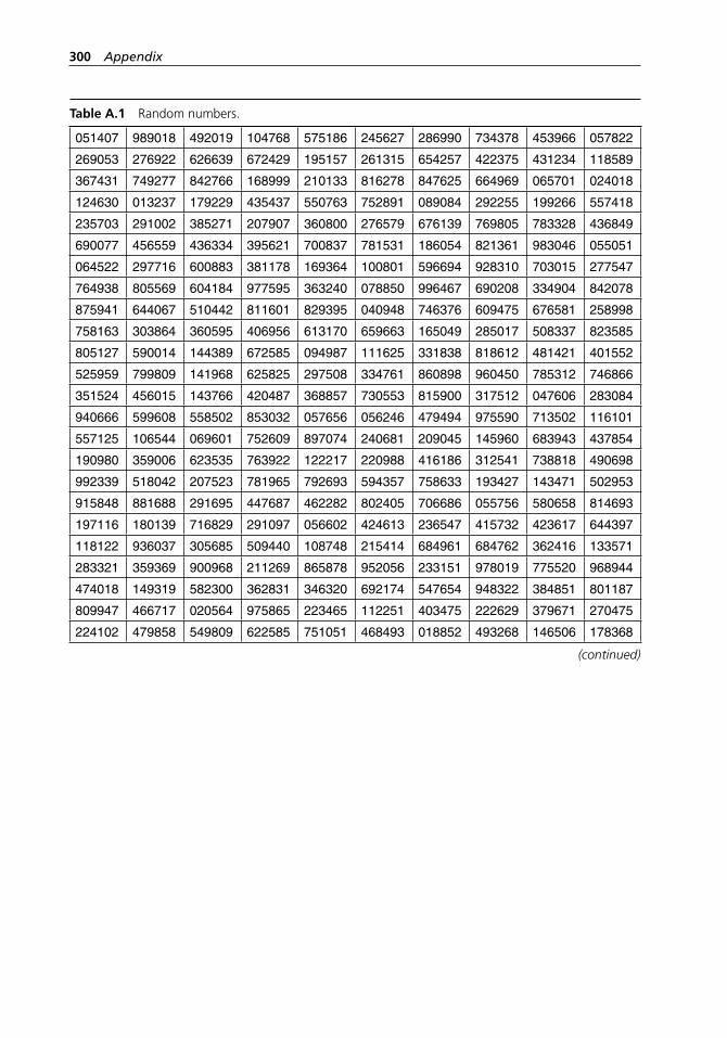
300 Appendix
Table A.1 Random numbers.
051407 989018 492019 104768 575186 245627 286990 734378 453966 057822
269053 276922 626639 672429 195157 261315 654257 422375 431234 118589
367431 749277 842766 168999 210133 816278 847625 664969 065701 024018
124630 013237 179229 435437 550763 752891 089084 292255 199266 557418
235703 291002 385271 207907 360800 276579 676139 769805 783328 436849
690077 456559 436334 395621 700837 781531 186054 821361 983046 055051
064522 297716 600883 381178 169364 100801 596694 928310 703015 277547
764938 805569 604184 977595 363240 078850 996467 690208 334904 842078
875941 644067 510442 811601 829395 040948 746376 609475 676581 258998
758163 303864 360595 406956 613170 659663 165049 285017 508337 823585
805127 590014 144389 672585 094987 111625 331838 818612 481421 401552
525959 799809 141968 625825 297508 334761 860898 960450 785312 746866
351524 456015 143766 420487 368857 730553 815900 317512 047606 283084
940666 599608 558502 853032 057656 056246 479494 975590 713502 116101
557125 106544 069601 752609 897074 240681 209045 145960 683943 437854
190980 359006 623535 763922 122217 220988 416186 312541 738818 490698
992339 518042 207523 781965 792693 594357 758633 193427 143471 502953
915848 881688 291695 447687 462282 802405 706686 055756 580658 814693
197116 180139 716829 291097 056602 424613 236547 415732 423617 644397
118122 936037 305685 509440 108748 215414 684961 684762 362416 133571
283321 359369 900968 211269 865878 952056 233151 978019 775520 968944
474018 149319 582300 362831 346320 692174 547654 948322 384851 801187
809947 466717 020564 975865 223465 112251 403475 222629 379671 270475
224102 479858 549809 622585 751051 468493 018852 493268 146506 178368
(continued)
H1277 ch12 App.indd 300H1277 ch12 App.indd 300 3/8/07 12:57:06 PM3/8/07 12:57:06 PM
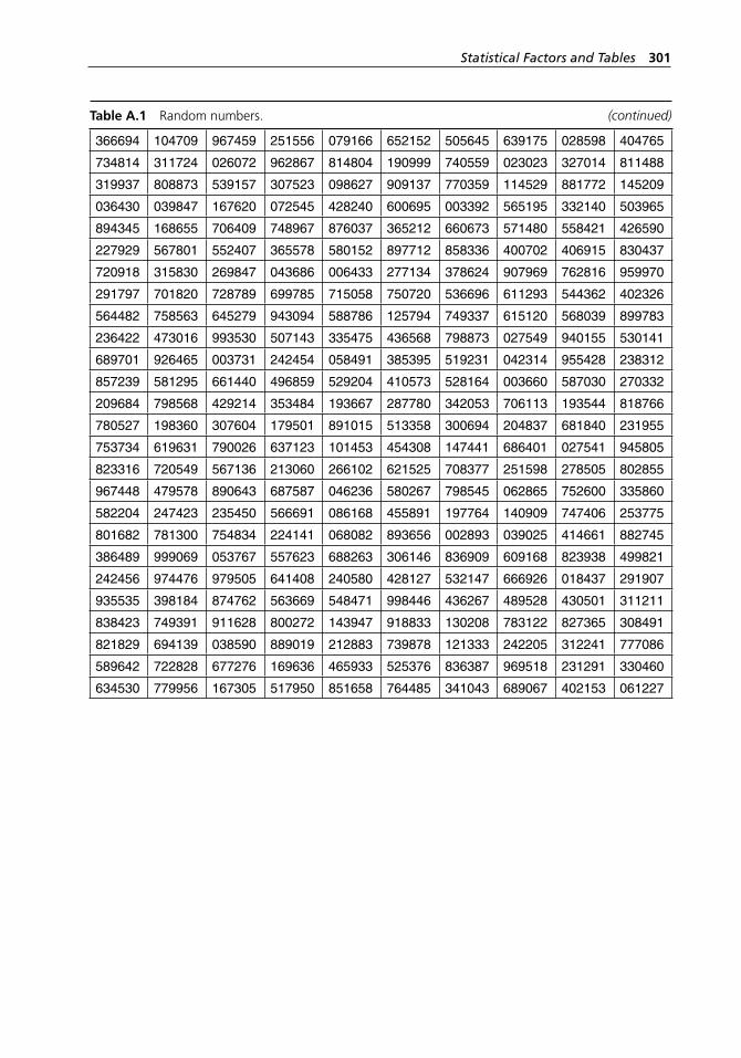
Statistical Factors and Tables 301
Table A.1 Random numbers.
366694 104709 967459 251556 079166 652152 505645 639175 028598 404765
734814 311724 026072 962867 814804 190999 740559 023023 327014 811488
319937 808873 539157 307523 098627 909137 770359 114529 881772 145209
036430 039847 167620 072545 428240 600695 003392 565195 332140 503965
894345 168655 706409 748967 876037 365212 660673 571480 558421 426590
227929 567801 552407 365578 580152 897712 858336 400702 406915 830437
720918 315830 269847 043686 006433 277134 378624 907969 762816 959970
291797 701820 728789 699785 715058 750720 536696 611293 544362 402326
564482 758563 645279 943094 588786 125794 749337 615120 568039 899783
236422 473016 993530 507143 335475 436568 798873 027549 940155 530141
689701 926465 003731 242454 058491 385395 519231 042314 955428 238312
857239 581295 661440 496859 529204 410573 528164 003660 587030 270332
209684 798568 429214 353484 193667 287780 342053 706113 193544 818766
780527 198360 307604 179501 891015 513358 300694 204837 681840 231955
753734 619631 790026 637123 101453 454308 147441 686401 027541 945805
823316 720549 567136 213060 266102 621525 708377 251598 278505 802855
967448 479578 890643 687587 046236 580267 798545 062865 752600 335860
582204 247423 235450 566691 086168 455891 197764 140909 747406 253775
801682 781300 754834 224141 068082 893656 002893 039025 414661 882745
386489 999069 053767 557623 688263 306146 836909 609168 823938 499821
242456 974476 979505 641408 240580 428127 532147 666926 018437 291907
935535 398184 874762 563669 548471 998446 436267 489528 430501 311211
838423 749391 911628 800272 143947 918833 130208 783122 827365 308491
821829 694139 038590 889019 212883 739878 121333 242205 312241 777086
589642 722828 677276 169636 465933 525376 836387 969518 231291 330460
634530 779956 167305 517950 851658 764485 341043 689067 402153 061227
(continued)
H1277 ch12 App.indd 301H1277 ch12 App.indd 301 3/8/07 12:57:06 PM3/8/07 12:57:06 PM
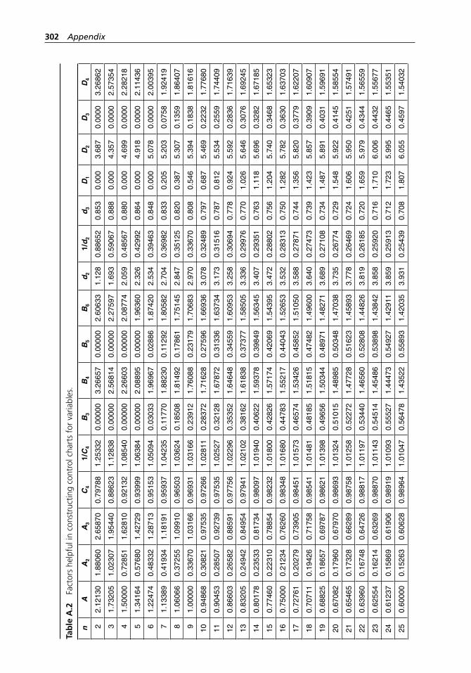
302 Appendix
Tab
le A
.2
Fact
ors
help
ful i
n co
nstr
uctin
g co
ntro
l cha
rts
for
varia
bles
.
nA
A2
A3
C4
1/C
4B
3B
4B
5B
6d
21/
d2
d3
D1
D2
D3
D4
22.
1213
01.
8806
02.
6587
00.
7978
81.
2533
20.
0000
03.
2665
70.
0000
02.
6063
31.
128
0.88
652
0.85
30.
000
3.68
70.
0000
3.26
862
31.
7320
51.
0230
71.
9544
00.
8862
31.
1283
80.
0000
02.
5681
40.
0000
02.
2759
71.
693
0.59
067
0.88
80.
000
4.35
70.
0000
2.57
354
41.
5000
00.
7285
11.
6281
00.
9213
21.
0854
00.
0000
02.
2660
30.
0000
02.
0877
42.
059
0.48
567
0.88
00.
000
4.69
90.
0000
2.28
218
51.
3416
40.
5768
01.
4272
90.
9399
91.
0638
40.
0000
02.
0889
50.
0000
01.
9636
02.
326
0.42
992
0.86
40.
000
4.91
80.
0000
2.11
436
61.
2247
40.
4833
21.
2871
30.
9515
31.
0509
40.
0303
31.
9696
70.
0288
61.
8742
02.
534
0.39
463
0.84
80.
000
5.07
80.
0000
2.00
395
71.
1338
90.
4193
41.
1819
10.
9593
71.
0423
50.
1177
01.
8823
00.
1129
21.
8058
22.
704
0.36
982
0.83
30.
205
5.20
30.
0758
1.92
419
81.
0606
60.
3725
51.
0991
00.
9650
31.
0362
40.
1850
81.
8149
20.
1786
11.
7514
52.
847
0.35
125
0.82
00.
387
5.30
70.
1359
1.86
407
91.
0000
00.
3367
01.
0316
60.
9693
11.
0316
60.
2391
21.
7608
80.
2317
91.
7068
32.
970
0.33
670
0.80
80.
546
5.39
40.
1838
1.81
616
100.
9486
80.
3082
10.
9753
50.
9726
61.
0281
10.
2837
21.
7162
80.
2759
61.
6693
63.
078
0.32
489
0.79
70.
687
5.46
90.
2232
1.77
680
110.
9045
30.
2850
70.
9273
90.
9753
51.
0252
70.
3212
81.
6787
20.
3133
61.
6373
43.
173
0.31
516
0.78
70.
812
5.53
40.
2559
1.74
409
120.
8660
30.
2658
20.
8859
10.
9775
61.
0229
60.
3535
21.
6464
80.
3455
91.
6095
33.
258
0.30
694
0.77
80.
924
5.59
20.
2836
1.71
639
130.
8320
50.
2494
20.
8495
40.
9794
11.
0210
20.
3816
21.
6183
80.
3737
71.
5850
53.
336
0.29
976
0.77
01.
026
5.64
60.
3076
1.69
245
140.
8017
80.
2353
30.
8173
40.
9809
71.
0194
00.
4062
21.
5937
80.
3984
91.
5634
53.
407
0.29
351
0.76
31.
118
5.69
60.
3282
1.67
185
150.
7746
00.
2231
00.
7885
40.
9823
21.
0180
00.
4282
61.
5717
40.
4206
91.
5439
53.
472
0.28
802
0.75
61.
204
5.74
00.
3468
1.65
323
160.
7500
00.
2123
40.
7626
00.
9834
81.
0168
00.
4478
31.
5521
70.
4404
31.
5265
33.
532
0.28
313
0.75
01.
282
5.78
20.
3630
1.63
703
170.
7276
10.
2027
90.
7390
50.
9845
11.
0157
30.
4657
41.
5342
60.
4585
21.
5105
03.
588
0.27
871
0.74
41.
356
5.82
00.
3779
1.62
207
180.
7071
10.
1942
60.
7175
80.
9854
11.
0148
10.
4818
51.
5181
50.
4748
21.
4960
03.
640
0.27
473
0.73
91.
423
5.85
70.
3909
1.60
907
190.
6882
50.
1865
70.
6978
70.
9862
11.
0139
80.
4965
61.
5034
40.
4897
11.
4827
13.
689
0.27
108
0.73
41.
487
5.89
10.
4031
1.59
691
200.
6708
20.
1796
00.
6797
00.
9869
31.
0132
40.
5101
51.
4898
50.
5034
81.
4703
83.
735
0.26
774
0.72
91.
548
5.92
20.
4145
1.58
554
210.
6546
50.
1732
80.
6628
90.
9875
81.
0125
80.
5227
21.
4772
80.
5162
31.
4589
33.
778
0.26
469
0.72
41.
606
5.95
00.
4251
1.57
491
220.
6396
00.
1674
80.
6472
60.
9881
71.
0119
70.
5344
01.
4656
00.
5280
81.
4482
63.
819
0.26
185
0.72
01.
659
5.97
90.
4344
1.56
559
230.
6255
40.
1621
40.
6326
90.
9887
01.
0114
30.
5451
41.
4548
60.
5389
81.
4384
23.
858
0.25
920
0.71
61.
710
6.00
60.
4432
1.55
677
240.
6123
70.
1586
90.
6190
60.
9891
91.
0109
30.
5552
71.
4447
30.
5492
71.
4291
13.
859
0.25
913
0.71
21.
723
5.99
50.
4465
1.55
351
250.
6000
00.
1526
30.
6062
80.
9896
41.
0104
70.
5647
81.
4352
20.
5589
31.
4203
53.
931
0.25
439
0.70
81.
807
6.05
50.
4597
1.54
032
H1277 ch12 App.indd 302H1277 ch12 App.indd 302 3/8/07 12:57:07 PM3/8/07 12:57:07 PM
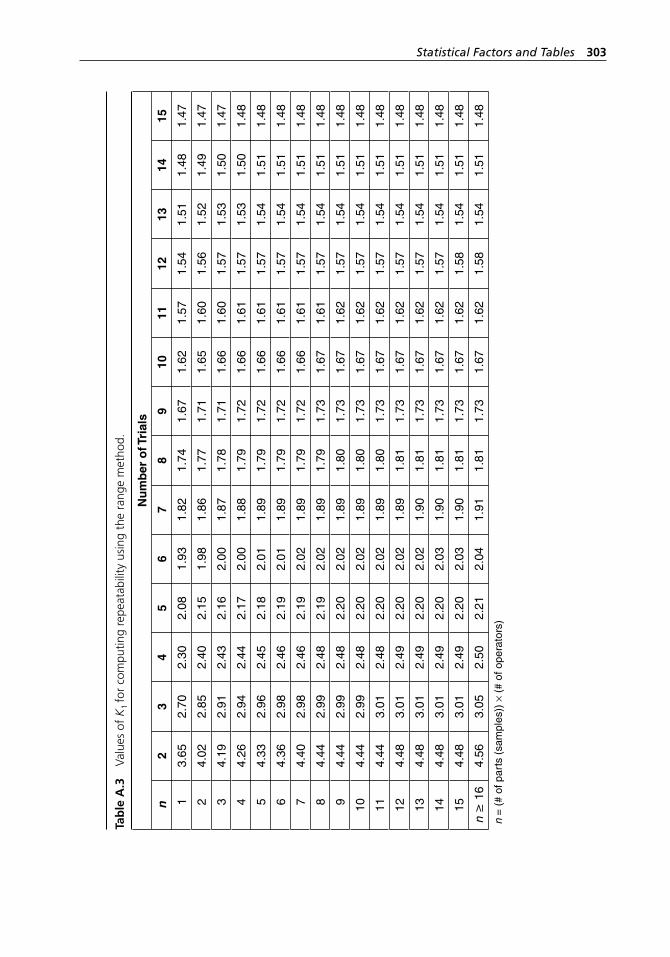
Statistical Factors and Tables 303
Tab
le A
.3
Valu
es o
f K
1 fo
r co
mpu
ting
repe
atab
ility
usi
ng t
he r
ange
met
hod.
Nu
mb
er o
f Tri
als
n2
34
56
78
910
1112
1314
15
13.
652.
702.
302.
081.
931.
821.
741.
671.
621.
571.
541.
511.
481.
47
24.
022.
852.
402.
151.
981.
861.
771.
711.
651.
601.
561.
521.
491.
47
34.
192.
912.
432.
162.
001.
871.
781.
711.
661.
601.
571.
531.
501.
47
44.
262.
942.
442.
172.
001.
881.
791.
721.
661.
611.
571.
531.
501.
48
54.
332.
962.
452.
182.
011.
891.
791.
721.
661.
611.
571.
541.
511.
48
64.
362.
982.
462.
192.
011.
891.
791.
721.
661.
611.
571.
541.
511.
48
74.
402.
982.
462.
192.
021.
891.
791.
721.
661.
611.
571.
541.
511.
48
84.
442.
992.
482.
192.
021.
891.
791.
731.
671.
611.
571.
541.
511.
48
94.
442.
992.
482.
202.
021.
891.
801.
731.
671.
621.
571.
541.
511.
48
104.
442.
992.
482.
202.
021.
891.
801.
731.
671.
621.
571.
541.
511.
48
114.
443.
012.
482.
202.
021.
891.
801.
731.
671.
621.
571.
541.
511.
48
124.
483.
012.
492.
202.
021.
891.
811.
731.
671.
621.
571.
541.
511.
48
134.
483.
012.
492.
202.
021.
901.
811.
731.
671.
621.
571.
541.
511.
48
144.
483.
012.
492.
202.
031.
901.
811.
731.
671.
621.
571.
541.
511.
48
154.
483.
012.
492.
202.
031.
901.
811.
731.
671.
621.
581.
541.
511.
48
n ≥
16
4.56
3.05
2.50
2.21
2.04
1.91
1.81
1.73
1.67
1.62
1.58
1.54
1.51
1.48
n =
(#
of p
arts
(sa
mpl
es))
× (
# of
ope
rato
rs)
H1277 ch12 App.indd 303H1277 ch12 App.indd 303 3/8/07 12:57:08 PM3/8/07 12:57:08 PM
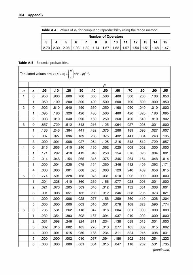
304 Appendix
Table A.5 Binomial probabilities.
Tabulated values are P X xn
xp px n x( ) ( )= =
⎛
⎝⎜⎜
⎞
⎠⎟⎟
− −1 .
p
n x .05 .10 .20 .30 .40 .50 .60 .70 .80 .90 .95
1 0 .950 .900 .800 .700 .600 .500 .400 .300 .200 .100 .050
1 .050 .100 .200 .300 .400 .500 .600 .700 .800 .900 .950
2 0 .902 .810 .640 .490 .360 .250 .160 .090 .040 .010 .003
1 .095 .180 .320 .420 .480 .500 .480 .420 .320 .180 .095
2 .003 .010 .040 .090 .160 .250 .360 .490 .640 .810 .902
3 0 .857 .729 .512 .343 .216 .125 .064 .027 .008 .001 .000
1 .136 .243 .384 .441 .432 .375 .288 .189 .096 .027 .007
2 .007 .027 .096 .189 .288 .375 .432 .441 .384 .243 .135
3 .000 .001 .008 .027 .064 .125 .216 .343 .512 .729 .857
4 0 .815 .656 .410 .240 .130 .062 .025 .008 .002 .000 .000
1 .171 .292 .410 .412 .346 .250 .154 .076 .026 .004 .001
2 .014 .048 .154 .265 .345 .375 .346 .264 .154 .048 .014
3 .000 .004 .025 .075 .154 .250 .346 .412 .409 .292 .171
4 .000 .000 .001 .008 .025 .063 .129 .240 .409 .656 .815
5 0 .774 .591 .328 .168 .078 .031 .010 .002 .000 .000 .000
1 .204 .328 .410 .360 .259 .156 .077 .028 .006 .001 .000
2 .021 .073 .205 .309 .346 .312 .230 .132 .051 .008 .001
3 .001 .008 .051 .132 .230 .312 .346 .308 .205 .073 .021
4 .000 .000 .006 .028 .077 .156 .259 .360 .410 .328 .204
5 .000 .000 .000 .003 .010 .031 .078 .168 .328 .590 .774
6 0 .735 .531 .262 .118 .047 .016 .004 .001 .000 .000 .000
1 .232 .354 .393 .302 .187 .094 .037 .010 .002 .000 .000
2 .031 .098 .246 .324 .311 .234 .138 .059 .015 .001 .000
3 .002 .015 .082 .185 .276 .313 .277 .185 .082 .015 .002
4 .000 .001 .015 .059 .138 .234 .311 .324 .246 .098 .031
5 .000 .000 .002 .010 .037 .094 .186 .302 .393 .354 .232
6 .000 .000 .000 .001 .004 .015 .047 .118 .262 .531 .735
Table A.4 Values of K2 for computing reproducibility using the range method.
Number of Operators
3 4 5 6 7 8 9 10 11 12 13 14 15
2.70 2.30 2.08 1.93 1.82 1.74 1.67 1.62 1.57 1.54 1.51 1.48 1.47
(continued)
H1277 ch12 App.indd 304H1277 ch12 App.indd 304 3/8/07 12:57:08 PM3/8/07 12:57:08 PM
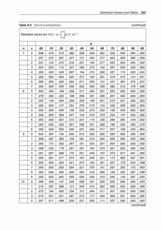
Statistical Factors and Tables 305
(continued)
Table A.5 Binomial probabilities.
Tabulated values are P X xn
xp px n x( ) ( )= =
⎛
⎝⎜⎜
⎞
⎠⎟⎟
− −1 .
p
n x .05 .10 .20 .30 .40 .50 .60 .70 .80 .90 .95
7 0 .698 .478 .210 .082 .028 .008 .002 .000 .000 .000 .000
1 .257 .372 .367 .247 .131 .055 .017 .004 .000 .000 .000
2 .041 .124 .275 .318 .261 .164 .077 .025 .004 .000 .000
3 .004 .023 .115 .227 .290 .273 .194 .097 .029 .003 .000
4 .000 .003 .029 .097 .194 .273 .290 .227 .115 .023 .004
5 .000 .000 .004 .025 .077 .164 .261 .318 .275 .124 .041
6 .000 .000 .000 .004 .017 .055 .131 .247 .367 .372 .257
7 .000 .000 .000 .000 .002 .008 .028 .082 .210 .478 .698
8 0 .663 .430 .168 .058 .017 .004 .001 .000 .000 .000 .000
1 .279 .383 .335 .198 .089 .031 .008 .001 .000 .000 .000
2 .052 .149 .294 .296 .209 .109 .041 .010 .001 .000 .000
3 .005 .033 .147 .254 .279 .219 .124 .048 .009 .000 .000
4 .000 .005 .046 .136 .232 .273 .232 .136 .046 .005 .000
5 .000 .000 .009 .047 .124 .219 .279 .254 .147 .033 .005
6 .000 .000 .001 .010 .041 .110 .209 .296 .294 .149 .052
7 .000 .000 .000 .001 .008 .031 .089 .198 .335 .383 .279
8 .000 .000 .000 .000 .001 .004 .017 .057 .168 .430 .664
9 0 .630 .387 .134 .040 .010 .002 .000 .000 .000 .000 .000
1 .298 .387 .302 .156 .061 .018 .004 .000 .000 .000 .000
2 .063 .172 .302 .267 .161 .070 .021 .004 .000 .000 .000
3 .008 .045 .176 .267 .251 .164 .074 .021 .003 .000 .000
4 .001 .007 .066 .172 .251 .246 .167 .073 .017 .001 .000
5 .000 .001 .017 .073 .167 .246 .251 .172 .066 .007 .001
6 .000 .000 .003 .021 .074 .164 .251 .267 .176 .045 .008
7 .000 .000 .000 .004 .021 .070 .161 .267 .302 .172 .063
8 .000 .000 .000 .000 .004 .018 .060 .156 .302 .387 .298
9 .000 .000 .000 .000 .000 .002 .010 .040 .134 .387 .630
10 0 .599 .349 .107 .028 .006 .001 .000 .000 .000 .000 .000
1 .315 .387 .268 .121 .040 .010 .002 .000 .000 .000 .000
2 .075 .194 .302 .234 .121 .044 .011 .001 .000 .000 .000
3 .010 .057 .201 .267 .215 .117 .042 .009 .001 .000 .000
4 .001 .011 .088 .200 .251 .205 .111 .037 .006 .000 .000
(continued)
(continued)
H1277 ch12 App.indd 305H1277 ch12 App.indd 305 3/8/07 12:57:09 PM3/8/07 12:57:09 PM
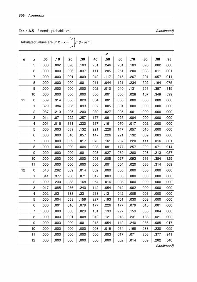
306 Appendix
Table A.5 Binomial probabilities.
Tabulated values are P X xn
xp px n x( ) ( )= =
⎛
⎝⎜⎜
⎞
⎠⎟⎟
− −1 .
p
n x .05 .10 .20 .30 .40 .50 .60 .70 .80 .90 .95
5 .000 .002 .026 .103 .201 .246 .201 .103 .026 .002 .000
6 .000 .000 .006 .037 .111 .205 .251 .200 .088 .011 .001
7 .000 .000 .001 .009 .042 .117 .215 .267 .201 .057 .011
8 .000 .000 .000 .001 .011 .044 .121 .234 .302 .194 .075
9 .000 .000 .000 .000 .002 .010 .040 .121 .268 .387 .315
10 .000 .000 .000 .000 .000 .001 .006 .028 .107 .349 .599
11 0 .569 .314 .086 .020 .004 .001 .000 .000 .000 .000 .000
1 .329 .384 .236 .093 .027 .005 .001 .000 .000 .000 .000
2 .087 .213 .295 .200 .089 .027 .005 .001 .000 .000 .000
3 .014 .071 .222 .257 .177 .081 .023 .004 .000 .000 .000
4 .001 .016 .111 .220 .237 .161 .070 .017 .002 .000 .000
5 .000 .003 .039 .132 .221 .226 .147 .057 .010 .000 .000
6 .000 .000 .010 .057 .147 .226 .221 .132 .039 .003 .000
7 .000 .000 .002 .017 .070 .161 .237 .220 .111 .016 .001
8 .000 .000 .000 .004 .023 .081 .177 .257 .222 .071 .014
9 .000 .000 .000 .001 .005 .027 .089 .200 .295 .213 .087
10 .000 .000 .000 .000 .001 .005 .027 .093 .236 .384 .329
11 .000 .000 .000 .000 .000 .001 .004 .020 .086 .314 .569
12 0 .540 .282 .069 .014 .002 .000 .000 .000 .000 .000 .000
1 .341 .377 .206 .071 .017 .003 .000 .000 .000 .000 .000
2 .099 .230 .283 .168 .064 .016 .003 .000 .000 .000 .000
3 :017 .085 .236 .240 .142 .054 .012 .002 .000 .000 .000
4 .002 .021 .133 .231 .213 .121 .042 .008 .001 .000 .000
5 .000 .004 .053 .159 .227 .193 .101 .030 .003 .000 .000
6 .000 .001 .016 .079 .177 .226 .177 .079 .016 .001 .000
7 .000 .000 .003 .029 .101 .193 .227 .159 .053 .004 .000
8 .000 .000 .001 .008 .042 .121 .213 .231 .133 .021 .002
9 .000 .000 .000 .001 .013 .054 .142 .240 .236 .085 .017
10 .000 .000 .000 .000 .003 .016 .064 .168 .283 .230 .099
11 .000 .000 .000 .000 .000 .003 .017 .071 .206 .377 .341
12 .000 .000 .000 .000 .000 .000 .002 .014 .069 .282 .540
(continued)
(continued)
H1277 ch12 App.indd 306H1277 ch12 App.indd 306 3/8/07 12:57:09 PM3/8/07 12:57:09 PM
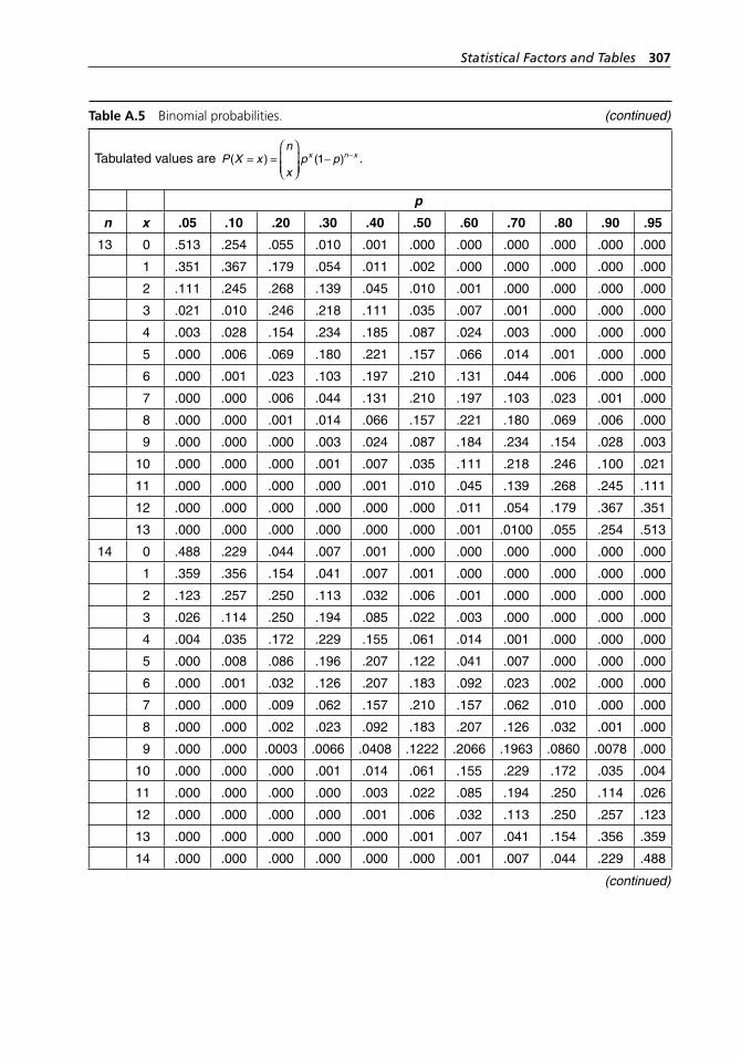
Statistical Factors and Tables 307
Table A.5 Binomial probabilities.
Tabulated values are P X xn
xp px n x( ) ( )= =
⎛
⎝⎜⎜
⎞
⎠⎟⎟
− −1 .
p
n x .05 .10 .20 .30 .40 .50 .60 .70 .80 .90 .95
13 0 .513 .254 .055 .010 .001 .000 .000 .000 .000 .000 .000
1 .351 .367 .179 .054 .011 .002 .000 .000 .000 .000 .000
2 .111 .245 .268 .139 .045 .010 .001 .000 .000 .000 .000
3 .021 .010 .246 .218 .111 .035 .007 .001 .000 .000 .000
4 .003 .028 .154 .234 .185 .087 .024 .003 .000 .000 .000
5 .000 .006 .069 .180 .221 .157 .066 .014 .001 .000 .000
6 .000 .001 .023 .103 .197 .210 .131 .044 .006 .000 .000
7 .000 .000 .006 .044 .131 .210 .197 .103 .023 .001 .000
8 .000 .000 .001 .014 .066 .157 .221 .180 .069 .006 .000
9 .000 .000 .000 .003 .024 .087 .184 .234 .154 .028 .003
10 .000 .000 .000 .001 .007 .035 .111 .218 .246 .100 .021
11 .000 .000 .000 .000 .001 .010 .045 .139 .268 .245 .111
12 .000 .000 .000 .000 .000 .000 .011 .054 .179 .367 .351
13 .000 .000 .000 .000 .000 .000 .001 .0100 .055 .254 .513
14 0 .488 .229 .044 .007 .001 .000 .000 .000 .000 .000 .000
1 .359 .356 .154 .041 .007 .001 .000 .000 .000 .000 .000
2 .123 .257 .250 .113 .032 .006 .001 .000 .000 .000 .000
3 .026 .114 .250 .194 .085 .022 .003 .000 .000 .000 .000
4 .004 .035 .172 .229 .155 .061 .014 .001 .000 .000 .000
5 .000 .008 .086 .196 .207 .122 .041 .007 .000 .000 .000
6 .000 .001 .032 .126 .207 .183 .092 .023 .002 .000 .000
7 .000 .000 .009 .062 .157 .210 .157 .062 .010 .000 .000
8 .000 .000 .002 .023 .092 .183 .207 .126 .032 .001 .000
9 .000 .000 .0003 .0066 .0408 .1222 .2066 .1963 .0860 .0078 .000
10 .000 .000 .000 .001 .014 .061 .155 .229 .172 .035 .004
11 .000 .000 .000 .000 .003 .022 .085 .194 .250 .114 .026
12 .000 .000 .000 .000 .001 .006 .032 .113 .250 .257 .123
13 .000 .000 .000 .000 .000 .001 .007 .041 .154 .356 .359
14 .000 .000 .000 .000 .000 .000 .001 .007 .044 .229 .488
(continued)
(continued)
H1277 ch12 App.indd 307H1277 ch12 App.indd 307 3/8/07 12:57:10 PM3/8/07 12:57:10 PM
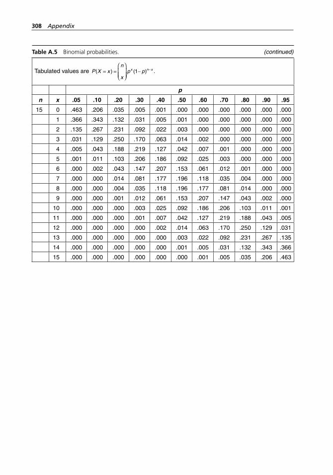
308 Appendix
Table A.5 Binomial probabilities.
Tabulated values are P X xn
xp px n x( ) ( )= =
⎛
⎝⎜⎜
⎞
⎠⎟⎟
− −1 .
p
n x .05 .10 .20 .30 .40 .50 .60 .70 .80 .90 .95
15 0 .463 .206 .035 .005 .001 .000 .000 .000 .000 .000 .000
1 .366 .343 .132 .031 .005 .001 .000 .000 .000 .000 .000
2 .135 .267 .231 .092 .022 .003 .000 .000 .000 .000 .000
3 .031 .129 .250 .170 .063 .014 .002 .000 .000 .000 .000
4 .005 .043 .188 .219 .127 .042 .007 .001 .000 .000 .000
5 .001 .011 .103 .206 .186 .092 .025 .003 .000 .000 .000
6 .000 .002 .043 .147 .207 .153 .061 .012 .001 .000 .000
7 .000 .000 .014 .081 .177 .196 .118 .035 .004 .000 .000
8 .000 .000 .004 .035 .118 .196 .177 .081 .014 .000 .000
9 .000 .000 .001 .012 .061 .153 .207 .147 .043 .002 .000
10 .000 .000 .000 .003 .025 .092 .186 .206 .103 .011 .001
11 .000 .000 .000 .001 .007 .042 .127 .219 .188 .043 .005
12 .000 .000 .000 .000 .002 .014 .063 .170 .250 .129 .031
13 .000 .000 .000 .000 .000 .003 .022 .092 .231 .267 .135
14 .000 .000 .000 .000 .000 .001 .005 .031 .132 .343 .366
15 .000 .000 .000 .000 .000 .000 .001 .005 .035 .206 .463
(continued)
H1277 ch12 App.indd 308H1277 ch12 App.indd 308 3/8/07 12:57:11 PM3/8/07 12:57:11 PM
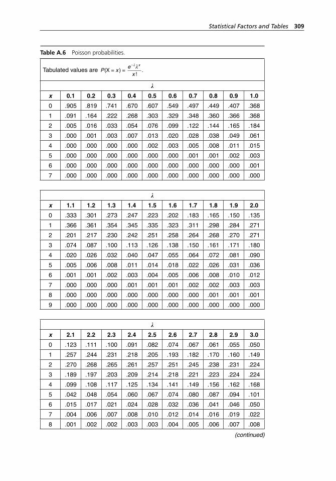
Statistical Factors and Tables 309
Table A.6 Poisson probabilities.
Tabulated values are P xe
x
x
(X = ) =− λ λ
!.
k
x 0.1 0.2 0.3 0.4 0.5 0.6 0.7 0.8 0.9 1.0
0 .905 .819 .741 .670 .607 .549 .497 .449 .407 .368
1 .091 .164 .222 .268 .303 .329 .348 .360 .366 .368
2 .005 .016 .033 .054 .076 .099 .122 .144 .165 .184
3 .000 .001 .003 .007 .013 .020 .028 .038 .049 .061
4 .000 .000 .000 .000 .002 .003 .005 .008 .011 .015
5 .000 .000 .000 .000 .000 .000 .001 .001 .002 .003
6 .000 .000 .000 .000 .000 .000 .000 .000 .000 .001
7 .000 .000 .000 .000 .000 .000 .000 .000 .000 .000
k
x 1.1 1.2 1.3 1.4 1.5 1.6 1.7 1.8 1.9 2.0
0 .333 .301 .273 .247 .223 .202 .183 .165 .150 .135
1 .366 .361 .354 .345 .335 .323 .311 .298 .284 .271
2 .201 .217 .230 .242 .251 .258 .264 .268 .270 .271
3 .074 .087 .100 .113 .126 .138 .150 .161 .171 .180
4 .020 .026 .032 .040 .047 .055 .064 .072 .081 .090
5 .005 .006 .008 .011 .014 .018 .022 .026 .031 .036
6 .001 .001 .002 .003 .004 .005 .006 .008 .010 .012
7 .000 .000 .000 .001 .001 .001 .002 .002 .003 .003
8 .000 .000 .000 .000 .000 .000 .000 .001 .001 .001
9 .000 .000 .000 .000 .000 .000 .000 .000 .000 .000
k
x 2.1 2.2 2.3 2.4 2.5 2.6 2.7 2.8 2.9 3.0
0 .123 .111 .100 .091 .082 .074 .067 .061 .055 .050
1 .257 .244 .231 .218 .205 .193 .182 .170 .160 .149
2 .270 .268 .265 .261 .257 .251 .245 .238 .231 .224
3 .189 .197 .203 .209 .214 .218 .221 .223 .224 .224
4 .099 .108 .117 .125 .134 .141 .149 .156 .162 .168
5 .042 .048 .054 .060 .067 .074 .080 .087 .094 .101
6 .015 .017 .021 .024 .028 .032 .036 .041 .046 .050
7 .004 .006 .007 .008 .010 .012 .014 .016 .019 .022
8 .001 .002 .002 .003 .003 .004 .005 .006 .007 .008
(continued)
H1277 ch12 App.indd 309H1277 ch12 App.indd 309 3/8/07 12:57:11 PM3/8/07 12:57:11 PM
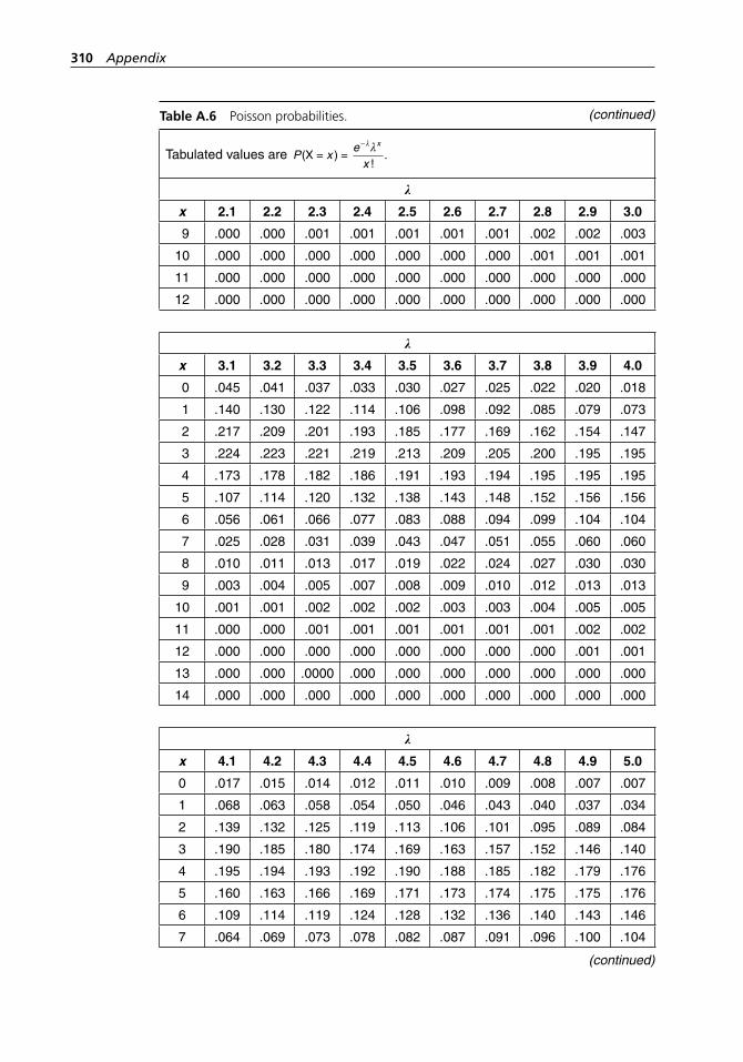
310 Appendix
Table A.6 Poisson probabilities.
Tabulated values are P xe
x
x
(X = ) =− λ λ
!.
k
x 2.1 2.2 2.3 2.4 2.5 2.6 2.7 2.8 2.9 3.0
9 .000 .000 .001 .001 .001 .001 .001 .002 .002 .003
10 .000 .000 .000 .000 .000 .000 .000 .001 .001 .001
11 .000 .000 .000 .000 .000 .000 .000 .000 .000 .000
12 .000 .000 .000 .000 .000 .000 .000 .000 .000 .000
k
x 3.1 3.2 3.3 3.4 3.5 3.6 3.7 3.8 3.9 4.0
0 .045 .041 .037 .033 .030 .027 .025 .022 .020 .018
1 .140 .130 .122 .114 .106 .098 .092 .085 .079 .073
2 .217 .209 .201 .193 .185 .177 .169 .162 .154 .147
3 .224 .223 .221 .219 .213 .209 .205 .200 .195 .195
4 .173 .178 .182 .186 .191 .193 .194 .195 .195 .195
5 .107 .114 .120 .132 .138 .143 .148 .152 .156 .156
6 .056 .061 .066 .077 .083 .088 .094 .099 .104 .104
7 .025 .028 .031 .039 .043 .047 .051 .055 .060 .060
8 .010 .011 .013 .017 .019 .022 .024 .027 .030 .030
9 .003 .004 .005 .007 .008 .009 .010 .012 .013 .013
10 .001 .001 .002 .002 .002 .003 .003 .004 .005 .005
11 .000 .000 .001 .001 .001 .001 .001 .001 .002 .002
12 .000 .000 .000 .000 .000 .000 .000 .000 .001 .001
13 .000 .000 .0000 .000 .000 .000 .000 .000 .000 .000
14 .000 .000 .000 .000 .000 .000 .000 .000 .000 .000
k
x 4.1 4.2 4.3 4.4 4.5 4.6 4.7 4.8 4.9 5.0
0 .017 .015 .014 .012 .011 .010 .009 .008 .007 .007
1 .068 .063 .058 .054 .050 .046 .043 .040 .037 .034
2 .139 .132 .125 .119 .113 .106 .101 .095 .089 .084
3 .190 .185 .180 .174 .169 .163 .157 .152 .146 .140
4 .195 .194 .193 .192 .190 .188 .185 .182 .179 .176
5 .160 .163 .166 .169 .171 .173 .174 .175 .175 .176
6 .109 .114 .119 .124 .128 .132 .136 .140 .143 .146
7 .064 .069 .073 .078 .082 .087 .091 .096 .100 .104
(continued)
(continued)
H1277 ch12 App.indd 310H1277 ch12 App.indd 310 3/8/07 12:57:12 PM3/8/07 12:57:12 PM
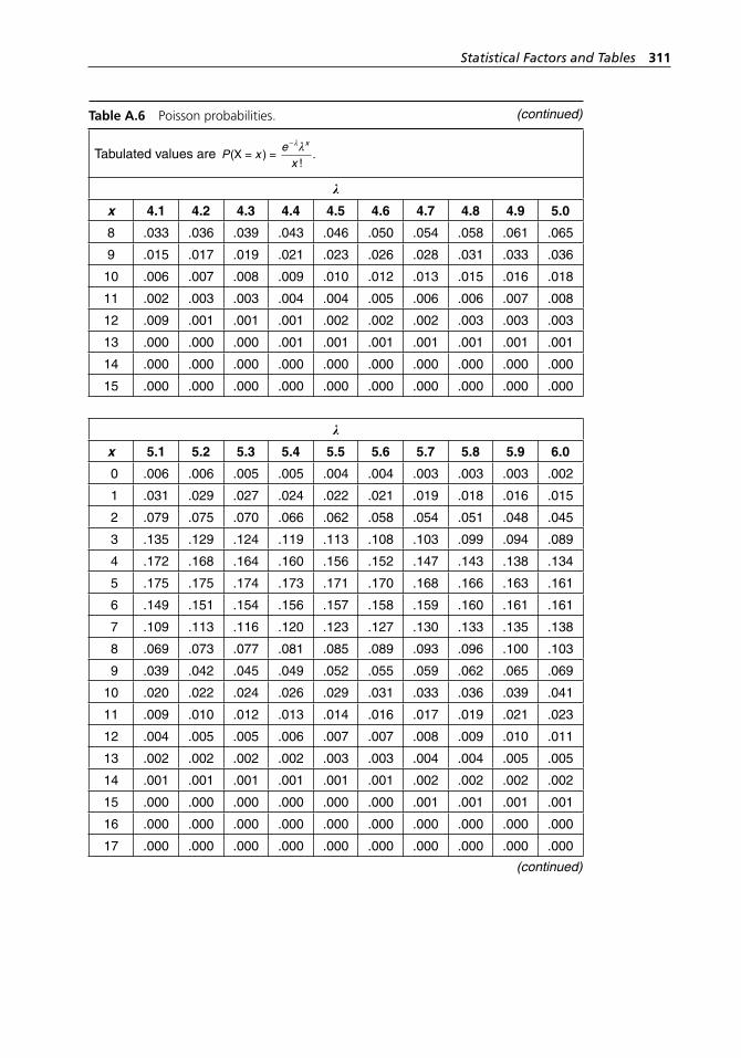
Statistical Factors and Tables 311
Table A.6 Poisson probabilities.
Tabulated values are P xe
x
x
(X = ) =− λ λ
!.
k
x 4.1 4.2 4.3 4.4 4.5 4.6 4.7 4.8 4.9 5.0
8 .033 .036 .039 .043 .046 .050 .054 .058 .061 .065
9 .015 .017 .019 .021 .023 .026 .028 .031 .033 .036
10 .006 .007 .008 .009 .010 .012 .013 .015 .016 .018
11 .002 .003 .003 .004 .004 .005 .006 .006 .007 .008
12 .009 .001 .001 .001 .002 .002 .002 .003 .003 .003
13 .000 .000 .000 .001 .001 .001 .001 .001 .001 .001
14 .000 .000 .000 .000 .000 .000 .000 .000 .000 .000
15 .000 .000 .000 .000 .000 .000 .000 .000 .000 .000
k
x 5.1 5.2 5.3 5.4 5.5 5.6 5.7 5.8 5.9 6.0
0 .006 .006 .005 .005 .004 .004 .003 .003 .003 .002
1 .031 .029 .027 .024 .022 .021 .019 .018 .016 .015
2 .079 .075 .070 .066 .062 .058 .054 .051 .048 .045
3 .135 .129 .124 .119 .113 .108 .103 .099 .094 .089
4 .172 .168 .164 .160 .156 .152 .147 .143 .138 .134
5 .175 .175 .174 .173 .171 .170 .168 .166 .163 .161
6 .149 .151 .154 .156 .157 .158 .159 .160 .161 .161
7 .109 .113 .116 .120 .123 .127 .130 .133 .135 .138
8 .069 .073 .077 .081 .085 .089 .093 .096 .100 .103
9 .039 .042 .045 .049 .052 .055 .059 .062 .065 .069
10 .020 .022 .024 .026 .029 .031 .033 .036 .039 .041
11 .009 .010 .012 .013 .014 .016 .017 .019 .021 .023
12 .004 .005 .005 .006 .007 .007 .008 .009 .010 .011
13 .002 .002 .002 .002 .003 .003 .004 .004 .005 .005
14 .001 .001 .001 .001 .001 .001 .002 .002 .002 .002
15 .000 .000 .000 .000 .000 .000 .001 .001 .001 .001
16 .000 .000 .000 .000 .000 .000 .000 .000 .000 .000
17 .000 .000 .000 .000 .000 .000 .000 .000 .000 .000
(continued)
(continued)
H1277 ch12 App.indd 311H1277 ch12 App.indd 311 3/8/07 12:57:12 PM3/8/07 12:57:12 PM
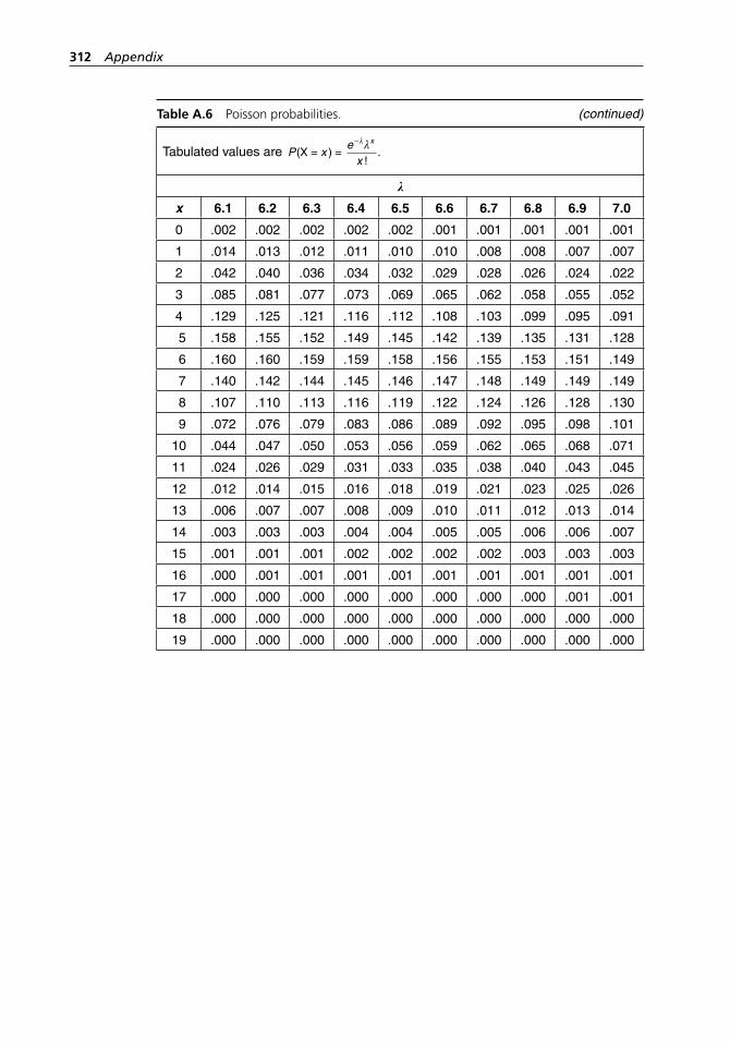
312 Appendix
Table A.6 Poisson probabilities.
Tabulated values are P xe
x
x
(X = ) =− λ λ
!.
k
x 6.1 6.2 6.3 6.4 6.5 6.6 6.7 6.8 6.9 7.0
0 .002 .002 .002 .002 .002 .001 .001 .001 .001 .001
1 .014 .013 .012 .011 .010 .010 .008 .008 .007 .007
2 .042 .040 .036 .034 .032 .029 .028 .026 .024 .022
3 .085 .081 .077 .073 .069 .065 .062 .058 .055 .052
4 .129 .125 .121 .116 .112 .108 .103 .099 .095 .091
5 .158 .155 .152 .149 .145 .142 .139 .135 .131 .128
6 .160 .160 .159 .159 .158 .156 .155 .153 .151 .149
7 .140 .142 .144 .145 .146 .147 .148 .149 .149 .149
8 .107 .110 .113 .116 .119 .122 .124 .126 .128 .130
9 .072 .076 .079 .083 .086 .089 .092 .095 .098 .101
10 .044 .047 .050 .053 .056 .059 .062 .065 .068 .071
11 .024 .026 .029 .031 .033 .035 .038 .040 .043 .045
12 .012 .014 .015 .016 .018 .019 .021 .023 .025 .026
13 .006 .007 .007 .008 .009 .010 .011 .012 .013 .014
14 .003 .003 .003 .004 .004 .005 .005 .006 .006 .007
15 .001 .001 .001 .002 .002 .002 .002 .003 .003 .003
16 .000 .001 .001 .001 .001 .001 .001 .001 .001 .001
17 .000 .000 .000 .000 .000 .000 .000 .000 .001 .001
18 .000 .000 .000 .000 .000 .000 .000 .000 .000 .000
19 .000 .000 .000 .000 .000 .000 .000 .000 .000 .000
(continued)
H1277 ch12 App.indd 312H1277 ch12 App.indd 312 3/8/07 12:57:13 PM3/8/07 12:57:13 PM
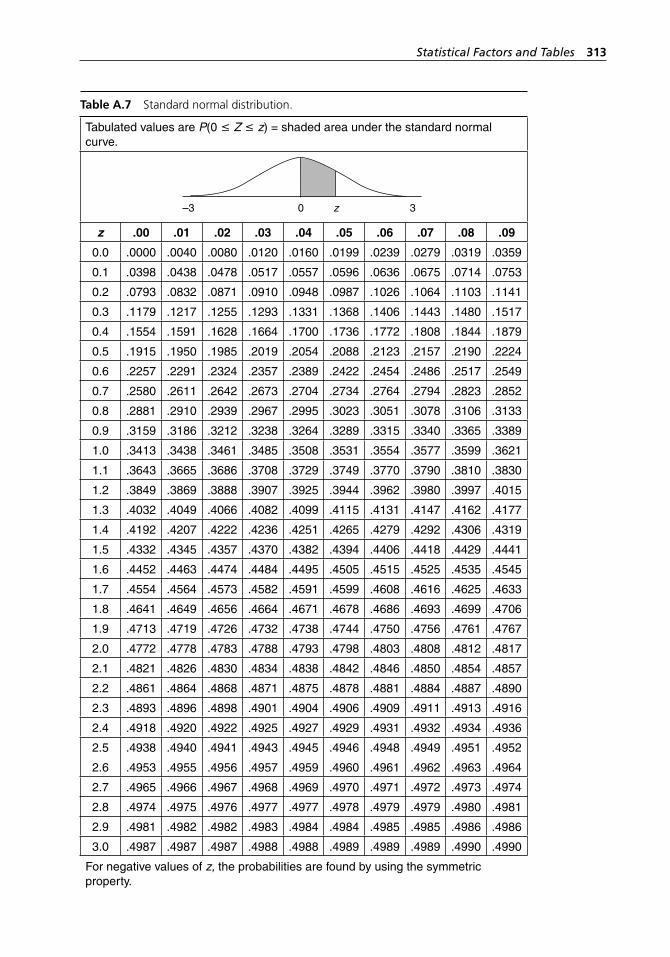
Statistical Factors and Tables 313
Table A.7 Standard normal distribution.
Tabulated values are P(0 ≤ Z ≤ z) = shaded area under the standard normal curve.
–3 0 z 3
z .00 .01 .02 .03 .04 .05 .06 .07 .08 .09
0.0 .0000 .0040 .0080 .0120 .0160 .0199 .0239 .0279 .0319 .0359
0.1 .0398 .0438 .0478 .0517 .0557 .0596 .0636 .0675 .0714 .0753
0.2 .0793 .0832 .0871 .0910 .0948 .0987 .1026 .1064 .1103 .1141
0.3 .1179 .1217 .1255 .1293 .1331 .1368 .1406 .1443 .1480 .1517
0.4 .1554 .1591 .1628 .1664 .1700 .1736 .1772 .1808 .1844 .1879
0.5 .1915 .1950 .1985 .2019 .2054 .2088 .2123 .2157 .2190 .2224
0.6 .2257 .2291 .2324 .2357 .2389 .2422 .2454 .2486 .2517 .2549
0.7 .2580 .2611 .2642 .2673 .2704 .2734 .2764 .2794 .2823 .2852
0.8 .2881 .2910 .2939 .2967 .2995 .3023 .3051 .3078 .3106 .3133
0.9 .3159 .3186 .3212 .3238 .3264 .3289 .3315 .3340 .3365 .3389
1.0 .3413 .3438 .3461 .3485 .3508 .3531 .3554 .3577 .3599 .3621
1.1 .3643 .3665 .3686 .3708 .3729 .3749 .3770 .3790 .3810 .3830
1.2 .3849 .3869 .3888 .3907 .3925 .3944 .3962 .3980 .3997 .4015
1.3 .4032 .4049 .4066 .4082 .4099 .4115 .4131 .4147 .4162 .4177
1.4 .4192 .4207 .4222 .4236 .4251 .4265 .4279 .4292 .4306 .4319
1.5 .4332 .4345 .4357 .4370 .4382 .4394 .4406 .4418 .4429 .4441
1.6 .4452 .4463 .4474 .4484 .4495 .4505 .4515 .4525 .4535 .4545
1.7 .4554 .4564 .4573 .4582 .4591 .4599 .4608 .4616 .4625 .4633
1.8 .4641 .4649 .4656 .4664 .4671 .4678 .4686 .4693 .4699 .4706
1.9 .4713 .4719 .4726 .4732 .4738 .4744 .4750 .4756 .4761 .4767
2.0 .4772 .4778 .4783 .4788 .4793 .4798 .4803 .4808 .4812 .4817
2.1 .4821 .4826 .4830 .4834 .4838 .4842 .4846 .4850 .4854 .4857
2.2 .4861 .4864 .4868 .4871 .4875 .4878 .4881 .4884 .4887 .4890
2.3 .4893 .4896 .4898 .4901 .4904 .4906 .4909 .4911 .4913 .4916
2.4 .4918 .4920 .4922 .4925 .4927 .4929 .4931 .4932 .4934 .4936
2.5 .4938 .4940 .4941 .4943 .4945 .4946 .4948 .4949 .4951 .4952
2.6 .4953 .4955 .4956 .4957 .4959 .4960 .4961 .4962 .4963 .4964
2.7 .4965 .4966 .4967 .4968 .4969 .4970 .4971 .4972 .4973 .4974
2.8 .4974 .4975 .4976 .4977 .4977 .4978 .4979 .4979 .4980 .4981
2.9 .4981 .4982 .4982 .4983 .4984 .4984 .4985 .4985 .4986 .4986
3.0 .4987 .4987 .4987 .4988 .4988 .4989 .4989 .4989 .4990 .4990
For negative values of z, the probabilities are found by using the symmetric property.
H1277 ch12 App.indd 313H1277 ch12 App.indd 313 3/8/07 12:57:13 PM3/8/07 12:57:13 PM
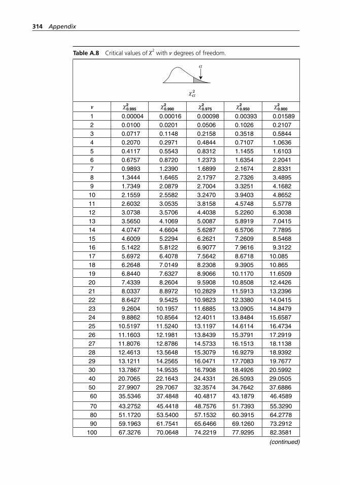
314 Appendix
Table A.8 Critical values of χ2 with ν degrees of freedom.
2
m χ20.995 χ2
0.990 χ20.975 χ2
0.950 χ20.900
1 0.00004 0.00016 0.00098 0.00393 0.015892 0.0100 0.0201 0.0506 0.1026 0.21073 0.0717 0.1148 0.2158 0.3518 0.58444 0.2070 0.2971 0.4844 0.7107 1.06365 0.4117 0.5543 0.8312 1.1455 1.61036 0.6757 0.8720 1.2373 1.6354 2.20417 0.9893 1.2390 1.6899 2.1674 2.83318 1.3444 1.6465 2.1797 2.7326 3.48959 1.7349 2.0879 2.7004 3.3251 4.168210 2.1559 2.5582 3.2470 3.9403 4.865211 2.6032 3.0535 3.8158 4.5748 5.577812 3.0738 3.5706 4.4038 5.2260 6.303813 3.5650 4.1069 5.0087 5.8919 7.041514 4.0747 4.6604 5.6287 6.5706 7.789515 4.6009 5.2294 6.2621 7.2609 8.546816 5.1422 5.8122 6.9077 7.9616 9.312217 5.6972 6.4078 7.5642 8.6718 10.08518 6.2648 7.0149 8.2308 9.3905 10.86519 6.8440 7.6327 8.9066 10.1170 11.650920 7.4339 8.2604 9.5908 10.8508 12.442621 8.0337 8.8972 10.2829 11.5913 13.239622 8.6427 9.5425 10.9823 12.3380 14.041523 9.2604 10.1957 11.6885 13.0905 14.847924 9.8862 10.8564 12.4011 13.8484 15.658725 10.5197 11.5240 13.1197 14.6114 16.473426 11.1603 12.1981 13.8439 15.3791 17.291927 11.8076 12.8786 14.5733 16.1513 18.113828 12.4613 13.5648 15.3079 16.9279 18.939229 13.1211 14.2565 16.0471 17.7083 19.767730 13.7867 14.9535 16.7908 18.4926 20.599240 20.7065 22.1643 24.4331 26.5093 29.050550 27.9907 29.7067 32.3574 34.7642 37.6886 60 35.5346 37.4848 40.4817 43.1879 46.4589
70 43.2752 45.4418 48.7576 51.7393 55.3290 80 51.1720 53.5400 57.1532 60.3915 64.2778 90 59.1963 61.7541 65.6466 69.1260 73.2912100 67.3276 70.0648 74.2219 77.9295 82.3581
(continued)
H1277 ch12 App.indd 314H1277 ch12 App.indd 314 3/8/07 12:57:14 PM3/8/07 12:57:14 PM
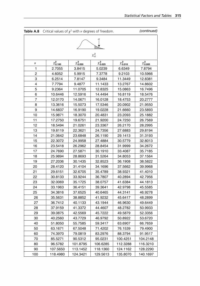
Statistical Factors and Tables 315
Table A.8 Critical values of χ2 with ν degrees of freedom.
2
m χ20.100 χ2
0.050 χ20.025 χ2
0.010 χ20.005
1 2.7055 3.8415 5.0239 6.6349 7.8794 2 4.6052 5.9915 7.3778 9.2103 10.5966 3 6.2514 7.8147 9.3484 11.3449 12.8381 4 7.7794 9.4877 11.1433 13.2767 14.8602 5 9.2364 11.0705 12.8325 15.0863 16.7496 6 10.6446 12.5916 14.4494 16.8119 18.5476 7 12.0170 14.0671 16.0128 18.4753 20.2777 8 13.3616 15.5073 17.5346 20.0902 21.9550 9 14.6837 16.9190 19.0228 21.6660 23.589310 15.9871 18.3070 20.4831 23.2093 25.188211 17.2750 19.6751 21.9200 24.7250 26.756912 18.5494 21.0261 23.3367 26.2170 28.299513 19.8119 22.3621 24.7356 27.6883 29.819414 21.0642 23.6848 26.1190 29.1413 31.319315 22.3072 24.9958 27.4884 30.5779 32.801316 23.5418 26.2962 28.8454 31.9999 34.267217 24.7690 27.5871 30.1910 33.4087 35.718518 25.9894 28.8693 31.5264 34.8053 37.156419 27.2036 30.1435 32.8523 36.1908 38.582220 28.4120 31.4104 34.1696 37.5662 39.996821 29.6151 32.6705 35.4789 38.9321 41.401022 30.8133 33.9244 36.7807 40.2894 42.795623 32.0069 35.1725 38.0757 41.6384 44.181324 33.1963 36.4151 39.3641 42.9798 45.558525 34.3816 37.6525 40.6465 44.3141 46.9278 26 35.5631 38.8852 41.9232 45.6417 48.2899 27 36.7412 40.1133 43.1944 46.9630 49.6449 28 37.9159 41.3372 44.4607 48.2782 50.9933 29 39.0875 42.5569 45.7222 49.5879 52.3356 30 40.2560 43.7729 46.9792 50.8922 53.6720 40 51.8050 55.7585 59.3417 63.6907 66.7659 50 63.1671 67.5048 71.4202 76.1539 79.4900 60 74.3970 79.0819 83.2976 88.3794 91.9517 70 85.5271 90.5312 95.0231 100.4251 104.2148 80 96.5782 101.8795 106.6285 112.3288 116.3210 90 107.5650 113.1452 118.1360 124.1162 128.2290100 118.4980 124.3421 129.5613 135.8070 140.1697
(continued)
H1277 ch12 App.indd 315H1277 ch12 App.indd 315 3/8/07 12:57:14 PM3/8/07 12:57:14 PM
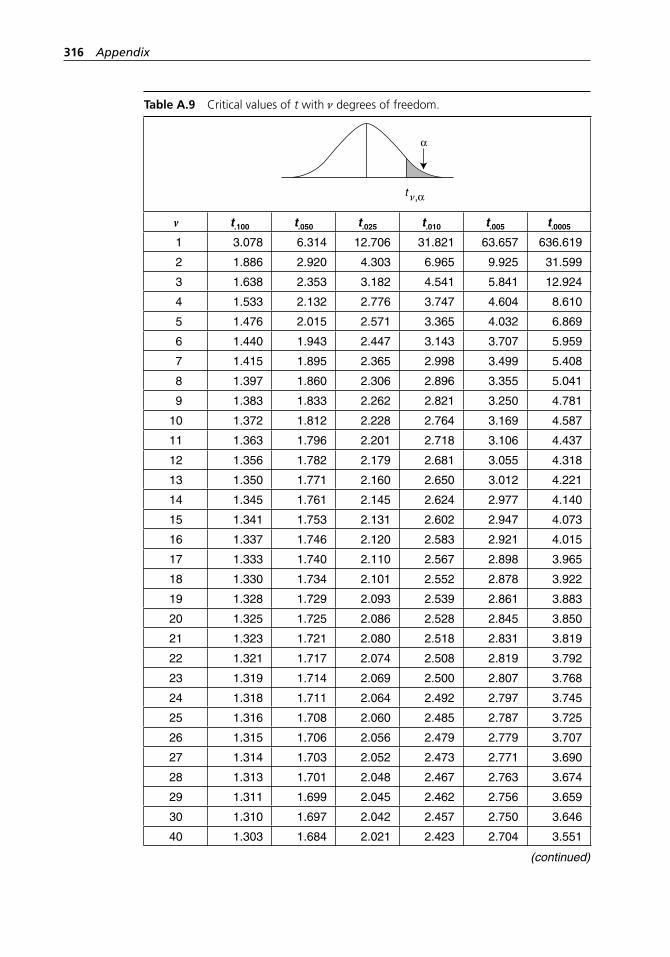
316 Appendix
(continued)
Table A.9 Critical values of t with ν degrees of freedom.
t ,
m t.100 t.050 t.025 t.010 t.005 t.0005
1 3.078 6.314 12.706 31.821 63.657 636.619
2 1.886 2.920 4.303 6.965 9.925 31.599
3 1.638 2.353 3.182 4.541 5.841 12.924
4 1.533 2.132 2.776 3.747 4.604 8.610
5 1.476 2.015 2.571 3.365 4.032 6.869
6 1.440 1.943 2.447 3.143 3.707 5.959
7 1.415 1.895 2.365 2.998 3.499 5.408
8 1.397 1.860 2.306 2.896 3.355 5.041
9 1.383 1.833 2.262 2.821 3.250 4.781
10 1.372 1.812 2.228 2.764 3.169 4.587
11 1.363 1.796 2.201 2.718 3.106 4.437
12 1.356 1.782 2.179 2.681 3.055 4.318
13 1.350 1.771 2.160 2.650 3.012 4.221
14 1.345 1.761 2.145 2.624 2.977 4.140
15 1.341 1.753 2.131 2.602 2.947 4.073
16 1.337 1.746 2.120 2.583 2.921 4.015
17 1.333 1.740 2.110 2.567 2.898 3.965
18 1.330 1.734 2.101 2.552 2.878 3.922
19 1.328 1.729 2.093 2.539 2.861 3.883
20 1.325 1.725 2.086 2.528 2.845 3.850
21 1.323 1.721 2.080 2.518 2.831 3.819
22 1.321 1.717 2.074 2.508 2.819 3.792
23 1.319 1.714 2.069 2.500 2.807 3.768
24 1.318 1.711 2.064 2.492 2.797 3.745
25 1.316 1.708 2.060 2.485 2.787 3.725
26 1.315 1.706 2.056 2.479 2.779 3.707
27 1.314 1.703 2.052 2.473 2.771 3.690
28 1.313 1.701 2.048 2.467 2.763 3.674
29 1.311 1.699 2.045 2.462 2.756 3.659
30 1.310 1.697 2.042 2.457 2.750 3.646
40 1.303 1.684 2.021 2.423 2.704 3.551
H1277 ch12 App.indd 316H1277 ch12 App.indd 316 3/8/07 12:57:15 PM3/8/07 12:57:15 PM
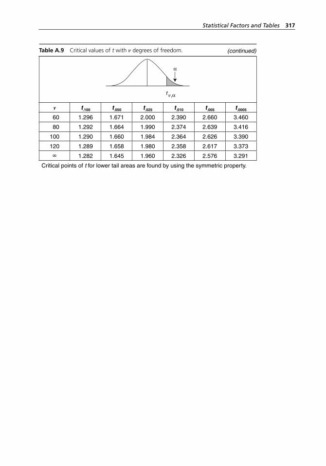
Statistical Factors and Tables 317
Table A.9 Critical values of t with ν degrees of freedom.
t ,
m t.100 t.050 t.025 t.010 t.005 t.0005
60 1.296 1.671 2.000 2.390 2.660 3.460
80 1.292 1.664 1.990 2.374 2.639 3.416
100 1.290 1.660 1.984 2.364 2.626 3.390
120 1.289 1.658 1.980 2.358 2.617 3.373
∞ 1.282 1.645 1.960 2.326 2.576 3.291
Critical points of t for lower tail areas are found by using the symmetric property.
(continued)
H1277 ch12 App.indd 317H1277 ch12 App.indd 317 3/8/07 12:57:16 PM3/8/07 12:57:16 PM
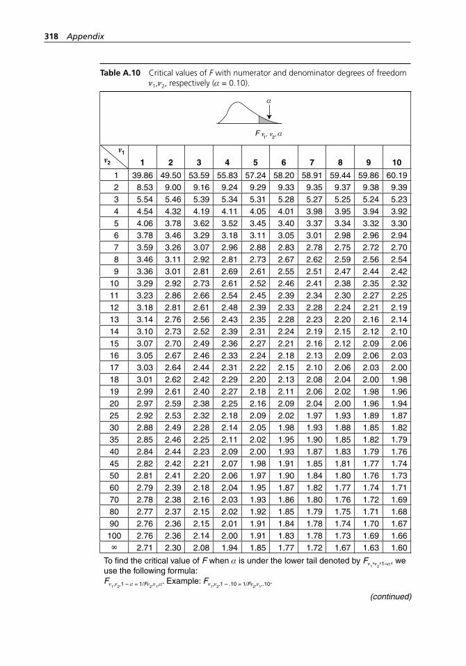
318 Appendix
Table A.10 Critical values of F with numerator and denominator degrees of freedom ν1,ν2, respectively (α = 0.10).
F , 1 2,
m1
m2 1 2 3 4 5 6 7 8 9 10
1 39.86 49.50 53.59 55.83 57.24 58.20 58.91 59.44 59.86 60.19 2 8.53 9.00 9.16 9.24 9.29 9.33 9.35 9.37 9.38 9.39 3 5.54 5.46 5.39 5.34 5.31 5.28 5.27 5.25 5.24 5.23 4 4.54 4.32 4.19 4.11 4.05 4.01 3.98 3.95 3.94 3.92 5 4.06 3.78 3.62 3.52 3.45 3.40 3.37 3.34 3.32 3.30 6 3.78 3.46 3.29 3.18 3.11 3.05 3.01 2.98 2.96 2.94 7 3.59 3.26 3.07 2.96 2.88 2.83 2.78 2.75 2.72 2.70 8 3.46 3.11 2.92 2.81 2.73 2.67 2.62 2.59 2.56 2.54 9 3.36 3.01 2.81 2.69 2.61 2.55 2.51 2.47 2.44 2.4210 3.29 2.92 2.73 2.61 2.52 2.46 2.41 2.38 2.35 2.3211 3.23 2.86 2.66 2.54 2.45 2.39 2.34 2.30 2.27 2.2512 3.18 2.81 2.61 2.48 2.39 2.33 2.28 2.24 2.21 2.1913 3.14 2.76 2.56 2.43 2.35 2.28 2.23 2.20 2.16 2.1414 3.10 2.73 2.52 2.39 2.31 2.24 2.19 2.15 2.12 2.1015 3.07 2.70 2.49 2.36 2.27 2.21 2.16 2.12 2.09 2.0616 3.05 2.67 2.46 2.33 2.24 2.18 2.13 2.09 2.06 2.0317 3.03 2.64 2.44 2.31 2.22 2.15 2.10 2.06 2.03 2.0018 3.01 2.62 2.42 2.29 2.20 2.13 2.08 2.04 2.00 1.9819 2.99 2.61 2.40 2.27 2.18 2.11 2.06 2.02 1.98 1.9620 2.97 2.59 2.38 2.25 2.16 2.09 2.04 2.00 1.96 1.9425 2.92 2.53 2.32 2.18 2.09 2.02 1.97 1.93 1.89 1.8730 2.88 2.49 2.28 2.14 2.05 1.98 1.93 1.88 1.85 1.8235 2.85 2.46 2.25 2.11 2.02 1.95 1.90 1.85 1.82 1.7940 2.84 2.44 2.23 2.09 2.00 1.93 1.87 1.83 1.79 1.7645 2.82 2.42 2.21 2.07 1.98 1.91 1.85 1.81 1.77 1.7450 2.81 2.41 2.20 2.06 1.97 1.90 1.84 1.80 1.76 1.7360 2.79 2.39 2.18 2.04 1.95 1.87 1.82 1.77 1.74 1.7170 2.78 2.38 2.16 2.03 1.93 1.86 1.80 1.76 1.72 1.6980 2.77 2.37 2.15 2.02 1.92 1.85 1.79 1.75 1.71 1.6890 2.76 2.36 2.15 2.01 1.91 1.84 1.78 1.74 1.70 1.67100 2.76 2.36 2.14 2.00 1.91 1.83 1.78 1.73 1.69 1.66∞ 2.71 2.30 2.08 1.94 1.85 1.77 1.72 1.67 1.63 1.60
To find the critical value of F when α is under the lower tail denoted by Fν1,ν2
,1–α, we use the following formula:Fν1,ν2,1 – α = 1/Fν2,ν1,α
. Example: Fν1,ν2,1 – .10 = 1/Fν2,ν1,.10.
(continued)
H1277 ch12 App.indd 318H1277 ch12 App.indd 318 3/8/07 12:57:16 PM3/8/07 12:57:16 PM
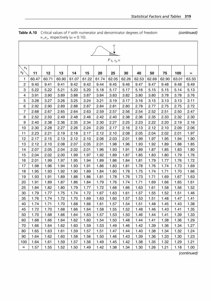
Statistical Factors and Tables 319
Table A.10 Critical values of F with numerator and denominator degrees of freedom ν1,ν2, respectively (α = 0.10).
F , 1 2,
m1
m2 11 12 13 14 15 20 25 30 40 50 75 100 ∞
1 60.47 60.71 60.90 61.07 61.22 61.74 62.05 62.26 62.53 62.69 62.90 63.01 63.33 2 9.40 9.41 9.41 9.42 9.42 9.44 9.45 9.46 9.47 9.47 9.48 9.48 9.49 3 5.22 5.22 5.21 5.20 5.20 5.18 5.17 5.17 5.16 5.15 5.15 5.14 5.13 4 3.91 3.90 3.89 3.88 3.87 3.84 3.83 3.82 3.80 3.80 3.78 3.78 3.76 5 3.28 3.27 3.26 3.25 3.24 3.21 3.19 3.17 3.16 3.15 3.13 3.13 3.11 6 2.92 2.90 2.89 2.88 2.87 2.84 2.81 2.80 2.78 2.77 2.75 2.75 2.72 7 2.68 2.67 2.65 2.64 2.63 2.59 2.57 2.56 2.54 2.52 2.51 2.50 2.47 8 2.52 2.50 2.49 2.48 2.46 2.42 2.40 2.38 2.36 2.35 2.33 2.32 2.30 9 2.40 2.38 2.36 2.35 2.34 2.30 2.27 2.25 2.23 2.22 2.20 2.19 2.1610 2.30 2.28 2.27 2.26 2.24 2.20 2.17 2.16 2.13 2.12 2.10 2.09 2.0611 2.23 2.21 2.19 2.18 2.17 2.12 2.10 2.08 2.05 2.04 2.02 2.01 1.9712 2.17 2.15 2.13 2.12 2.10 2.06 2.03 2.01 1.99 1.97 1.95 1.94 1.9013 2.12 2.10 2.08 2.07 2.05 2.01 1.98 1.96 1.93 1.92 1.89 1.88 1.8514 2.07 2.05 2.04 2.02 2.01 1.96 1.93 1.91 1.89 1.87 1.85 1.83 1.8015 2.04 2.02 2.00 1.99 1.97 1.92 1.89 1.87 1.85 1.83 1.80 1.79 1.7616 2.01 1.99 1.97 1.95 1.94 1.89 1.86 1.84 1.81 1.79 1.77 1.76 1.7217 1.98 1.96 1.94 1.93 1.91 1.86 1.83 1.81 1.78 1.76 1.74 1.73 1.6918 1.95 1.93 1.92 1.90 1.89 1.84 1.80 1.78 1.75 1.74 1.71 1.70 1.6619 1.93 1.91 1.89 1.88 1.86 1.81 1.78 1.76 1.73 1.71 1.69 1.67 1.6320 1.91 1.89 1.87 1.86 1.84 1.79 1.76 1.74 1.71 1.69 1.66 1.65 1.6125 1.84 1.82 1.80 1.79 1.77 1.72 1.68 1.66 1.63 1.61 1.58 1.56 1.5230 1.79 1.77 1.75 1.74 1.72 1.67 1.63 1.61 1.57 1.55 1.52 1.51 1.4635 1.76 1.74 1.72 1.70 1.69 1.63 1.60 1.57 1.53 1.51 1.48 1.47 1.4140 1.74 1.71 1.70 1.68 1.66 1.61 1.57 1.54 1.51 1.48 1.45 1.43 1.3845 1.72 1.70 1.68 1.66 1.64 1.58 1.55 1.52 1.48 1.46 1.43 1.41 1.3550 1.70 1.68 1.66 1.64 1.63 1.57 1.53 1.50 1.46 1.44 1.41 1.39 1.3360 1.68 1.66 1.64 1.62 1.60 1.54 1.50 1.48 1.44 1.41 1.38 1.36 1.2970 1.66 1.64 1.62 1.60 1.59 1.53 1.49 1.46 1.42 1.39 1.36 1.34 1.2780 1.65 1.63 1.61 1.59 1.57 1.51 1.47 1.44 1.40 1.38 1.34 1.32 1.2490 1.64 1.62 1.60 1.58 1.56 1.50 1.46 1.43 1.39 1.36 1.33 1.30 1.23100 1.64 1.61 1.59 1.57 1.56 1.49 1.45 1.42 1.38 1.35 1.32 1.29 1.21∞ 1.57 1.55 1.52 1.50 1.49 1.42 1.38 1.34 1.30 1.26 1.21 1.18 1.00
(continued)
(continued)
H1277 ch12 App.indd 319H1277 ch12 App.indd 319 3/8/07 12:57:16 PM3/8/07 12:57:16 PM
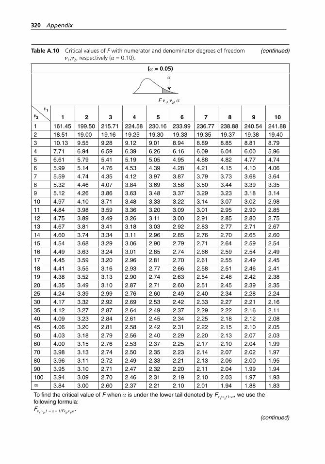
320 Appendix
Table A.10 Critical values of F with numerator and denominator degrees of freedom ν1,ν2, respectively (α = 0.10).
(α = 0.05)
F 1, 2,
m1
m2 1 2 3 4 5 6 7 8 9 10
1 161.45 199.50 215.71 224.58 230.16 233.99 236.77 238.88 240.54 241.882 18.51 19.00 19.16 19.25 19.30 19.33 19.35 19.37 19.38 19.403 10.13 9.55 9.28 9.12 9.01 8.94 8.89 8.85 8.81 8.794 7.71 6.94 6.59 6.39 6.26 6.16 6.09 6.04 6.00 5.965 6.61 5.79 5.41 5.19 5.05 4.95 4.88 4.82 4.77 4.746 5.99 5.14 4.76 4.53 4.39 4.28 4.21 4.15 4.10 4.067 5.59 4.74 4.35 4.12 3.97 3.87 3.79 3.73 3.68 3.648 5.32 4.46 4.07 3.84 3.69 3.58 3.50 3.44 3.39 3.359 5.12 4.26 3.86 3.63 3.48 3.37 3.29 3.23 3.18 3.1410 4.97 4.10 3.71 3.48 3.33 3.22 3.14 3.07 3.02 2.9811 4.84 3.98 3.59 3.36 3.20 3.09 3.01 2.95 2.90 2.8512 4.75 3.89 3.49 3.26 3.11 3.00 2.91 2.85 2.80 2.7513 4.67 3.81 3.41 3.18 3.03 2.92 2.83 2.77 2.71 2.6714 4.60 3.74 3.34 3.11 2.96 2.85 2.76 2.70 2.65 2.6015 4.54 3.68 3.29 3.06 2.90 2.79 2.71 2.64 2.59 2.5416 4.49 3.63 3.24 3.01 2.85 2.74 2.66 2.59 2.54 2.4917 4.45 3.59 3.20 2.96 2.81 2.70 2.61 2.55 2.49 2.4518 4.41 3.55 3.16 2.93 2.77 2.66 2.58 2.51 2.46 2.4119 4.38 3.52 3.13 2.90 2.74 2.63 2.54 2.48 2.42 2.3820 4.35 3.49 3.10 2.87 2.71 2.60 2.51 2.45 2.39 2.3525 4.24 3.39 2.99 2.76 2.60 2.49 2.40 2.34 2.28 2.2430 4.17 3.32 2.92 2.69 2.53 2.42 2.33 2.27 2.21 2.1635 4.12 3.27 2.87 2.64 2.49 2.37 2.29 2.22 2.16 2.1140 4.09 3.23 2.84 2.61 2.45 2.34 2.25 2.18 2.12 2.0845 4.06 3.20 2.81 2.58 2.42 2.31 2.22 2.15 2.10 2.0550 4.03 3.18 2.79 2.56 2.40 2.29 2.20 2.13 2.07 2.0360 4.00 3.15 2.76 2.53 2.37 2.25 2.17 2.10 2.04 1.9970 3.98 3.13 2.74 2.50 2.35 2.23 2.14 2.07 2.02 1.9780 3.96 3.11 2.72 2.49 2.33 2.21 2.13 2.06 2.00 1.9590 3.95 3.10 2.71 2.47 2.32 2.20 2.11 2.04 1.99 1.94100 3.94 3.09 2.70 2.46 2.31 2.19 2.10 2.03 1.97 1.93∞ 3.84 3.00 2.60 2.37 2.21 2.10 2.01 1.94 1.88 1.83
To find the critical value of F when α is under the lower tail denoted by Fν1,ν2
,1–α, we use the following formula:Fν1,ν2,1 – α = 1/Fν2,ν1,α
.
(continued)
(continued)
H1277 ch12 App.indd 320H1277 ch12 App.indd 320 3/8/07 12:57:17 PM3/8/07 12:57:17 PM
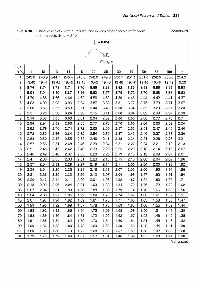
Statistical Factors and Tables 321
Table A.10 Critical values of F with numerator and denominator degrees of freedom ν1,ν2, respectively (α = 0.10).
(α = 0.05)
F 1, 2,
m1
m2 11 12 13 14 15 20 25 30 40 50 75 100 ∞
1 243.0 243.9 244.7 245.4 246.0 248.0 249.3 250.1 251.1 251.8 252.6 253.0 254.3 2 19.40 19.41 19.42 19.42 19.43 19.45 19.46 19.46 19.47 19.48 19.48 19.49 19.50 3 8.76 8.74 8.73 8.71 8.70 8.66 8.63 8.62 8.59 8.58 8.56 8.55 8.53 4 5.94 5.91 5.89 5.87 5.86 5.80 5.77 5.75 5.72 5.70 5.68 5.66 5.63 5 4.70 4.68 4.66 4.64 4.62 4.56 4.52 4.50 4.46 4.44 4.42 4.41 4.37 6 4.03 4.00 3.98 3.96 3.94 3.87 3.83 3.81 3.77 3.75 3.73 3.71 3.67 7 3.60 3.57 3.55 3.53 3.51 3.44 3.40 3.38 3.34 3.32 3.29 3.27 3.23 8 3.31 3.28 3.26 3.24 3.22 3.15 3.11 3.08 3.04 3.02 2.99 2.97 2.93 9 3.10 3.07 3.05 3.03 3.01 2.94 2.89 2.86 2.83 2.80 2.77 2.76 2.7110 2.94 2.91 2.89 2.86 2.85 2.77 2.73 2.70 2.66 2.64 2.60 2.59 2.5411 2.82 2.79 2.76 2.74 2.72 2.65 2.60 2.57 2.53 2.51 2.47 2.46 2.4012 2.72 2.69 2.66 2.64 2.62 2.54 2.50 2.47 2.43 2.40 2.37 2.35 2.3013 2.63 2.60 2.58 2.55 2.53 2.46 2.41 2.38 2.34 2.31 2.28 2.26 2.2114 2.57 2.53 2.51 2.48 2.46 2.39 2.34 2.31 2.27 2.24 2.21 2.19 2.1315 2.51 2.48 2.45 2.42 2.40 2.33 2.28 2.25 2.20 2.18 2.14 2.12 2.0716 2.46 2.42 2.40 2.37 2.35 2.28 2.23 2.19 2.15 2.12 2.09 2.07 2.0117 2.41 2.38 2.35 2.33 2.31 2.23 2.18 2.15 2.10 2.08 2.04 2.02 1.9618 2.37 2.34 2.31 2.29 2.27 2.19 2.14 2.11 2.06 2.04 2.00 1.98 1.9219 2.34 2.31 2.28 2.26 2.23 2.16 2.11 2.07 2.03 2.00 1.96 1.94 1.8820 2.31 2.28 2.25 2.22 2.20 2.12 2.07 2.04 1.99 1.97 1.93 1.91 1.8425 2.20 2.16 2.14 2.11 2.09 2.01 1.96 1.92 1.87 1.84 1.80 1.78 1.7130 2.13 2.09 2.06 2.04 2.01 1.93 1.88 1.84 1.79 1.76 1.72 1.70 1.6235 2.07 2.04 2.01 1.99 1.96 1.88 1.82 1.79 1.74 1.70 1.66 1.63 1.5640 2.04 2.00 1.97 1.95 1.92 1.84 1.78 1.74 1.69 1.66 1.61 1.59 1.5145 2.01 1.97 1.94 1.92 1.89 1.81 1.75 1.71 1.66 1.63 1.58 1.55 1.4750 1.99 1.95 1.92 1.89 1.87 1.78 1.73 1.69 1.63 1.60 1.55 1.52 1.4460 1.95 1.92 1.89 1.86 1.84 1.75 1.69 1.65 1.59 1.56 1.51 1.48 1.3970 1.93 1.89 1.86 1.84 1.81 1.72 1.66 1.62 1.57 1.53 1.48 1.45 1.3580 1.91 1.88 1.84 1.82 1.79 1.70 1.64 1.60 1.54 1.51 1.45 1.43 1.3290 1.90 1.86 1.83 1.80 1.78 1.69 1.63 1.59 1.53 1.49 1.44 1.41 1.30100 1.89 1.85 1.82 1.79 1.77 1.68 1.62 1.57 1.52 1.48 1.42 1.39 1.28∞ 1.79 1.75 1.72 1.69 1.67 1.57 1.51 1.46 1.39 1.35 1.28 1.24 1.00
(continued)
(continued)
H1277 ch12 App.indd 321H1277 ch12 App.indd 321 3/8/07 12:57:18 PM3/8/07 12:57:18 PM
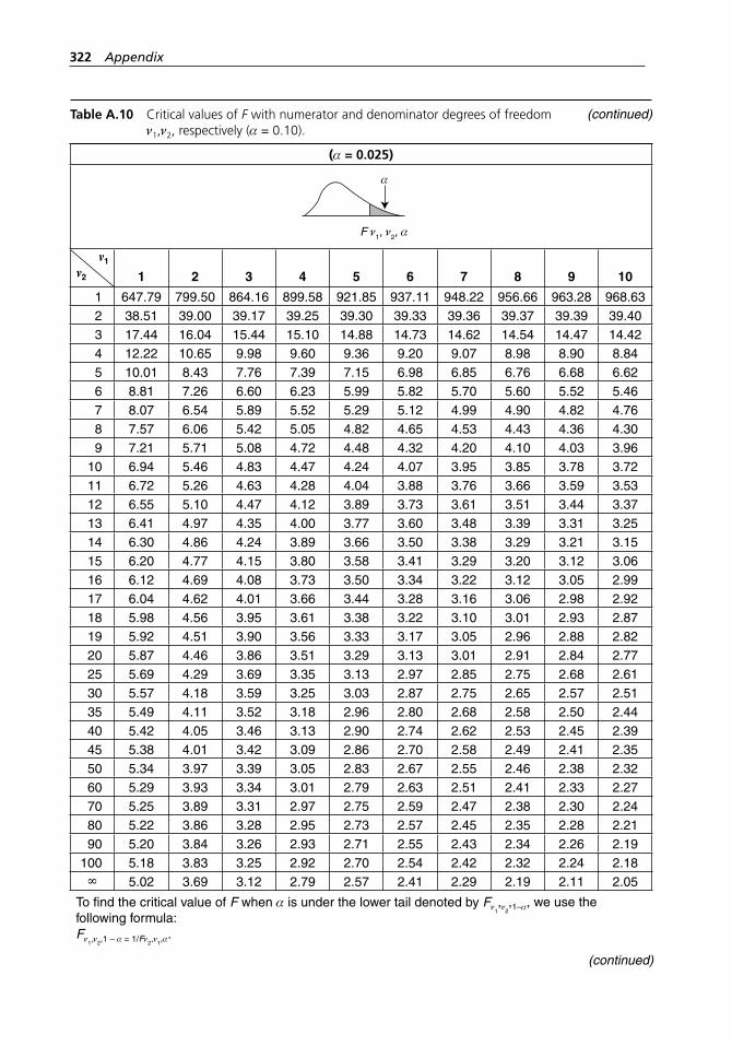
322 Appendix
Table A.10 Critical values of F with numerator and denominator degrees of freedom ν1,ν2, respectively (α = 0.10).
(α = 0.025)
F 1, 2,
m1
m2 1 2 3 4 5 6 7 8 9 10
1 647.79 799.50 864.16 899.58 921.85 937.11 948.22 956.66 963.28 968.63 2 38.51 39.00 39.17 39.25 39.30 39.33 39.36 39.37 39.39 39.40 3 17.44 16.04 15.44 15.10 14.88 14.73 14.62 14.54 14.47 14.42 4 12.22 10.65 9.98 9.60 9.36 9.20 9.07 8.98 8.90 8.84 5 10.01 8.43 7.76 7.39 7.15 6.98 6.85 6.76 6.68 6.62 6 8.81 7.26 6.60 6.23 5.99 5.82 5.70 5.60 5.52 5.46 7 8.07 6.54 5.89 5.52 5.29 5.12 4.99 4.90 4.82 4.76 8 7.57 6.06 5.42 5.05 4.82 4.65 4.53 4.43 4.36 4.30 9 7.21 5.71 5.08 4.72 4.48 4.32 4.20 4.10 4.03 3.9610 6.94 5.46 4.83 4.47 4.24 4.07 3.95 3.85 3.78 3.7211 6.72 5.26 4.63 4.28 4.04 3.88 3.76 3.66 3.59 3.5312 6.55 5.10 4.47 4.12 3.89 3.73 3.61 3.51 3.44 3.3713 6.41 4.97 4.35 4.00 3.77 3.60 3.48 3.39 3.31 3.2514 6.30 4.86 4.24 3.89 3.66 3.50 3.38 3.29 3.21 3.1515 6.20 4.77 4.15 3.80 3.58 3.41 3.29 3.20 3.12 3.0616 6.12 4.69 4.08 3.73 3.50 3.34 3.22 3.12 3.05 2.9917 6.04 4.62 4.01 3.66 3.44 3.28 3.16 3.06 2.98 2.9218 5.98 4.56 3.95 3.61 3.38 3.22 3.10 3.01 2.93 2.8719 5.92 4.51 3.90 3.56 3.33 3.17 3.05 2.96 2.88 2.8220 5.87 4.46 3.86 3.51 3.29 3.13 3.01 2.91 2.84 2.7725 5.69 4.29 3.69 3.35 3.13 2.97 2.85 2.75 2.68 2.6130 5.57 4.18 3.59 3.25 3.03 2.87 2.75 2.65 2.57 2.5135 5.49 4.11 3.52 3.18 2.96 2.80 2.68 2.58 2.50 2.4440 5.42 4.05 3.46 3.13 2.90 2.74 2.62 2.53 2.45 2.3945 5.38 4.01 3.42 3.09 2.86 2.70 2.58 2.49 2.41 2.3550 5.34 3.97 3.39 3.05 2.83 2.67 2.55 2.46 2.38 2.3260 5.29 3.93 3.34 3.01 2.79 2.63 2.51 2.41 2.33 2.2770 5.25 3.89 3.31 2.97 2.75 2.59 2.47 2.38 2.30 2.2480 5.22 3.86 3.28 2.95 2.73 2.57 2.45 2.35 2.28 2.2190 5.20 3.84 3.26 2.93 2.71 2.55 2.43 2.34 2.26 2.19
100 5.18 3.83 3.25 2.92 2.70 2.54 2.42 2.32 2.24 2.18∞ 5.02 3.69 3.12 2.79 2.57 2.41 2.29 2.19 2.11 2.05
To find the critical value of F when α is under the lower tail denoted by Fν1,ν2
,1–α, we use the following formula:Fν1,ν2,1 – α = 1/Fν2,ν1,α
.
(continued)
(continued)
H1277 ch12 App.indd 322H1277 ch12 App.indd 322 3/8/07 12:57:19 PM3/8/07 12:57:19 PM
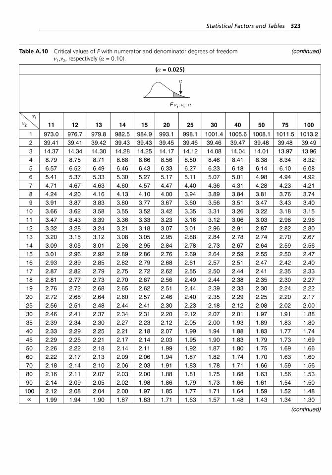
Statistical Factors and Tables 323
Table A.10 Critical values of F with numerator and denominator degrees of freedom ν1,ν2, respectively (α = 0.10).
(α = 0.025)
F 1, 2,
m1
m2 11 12 13 14 15 20 25 30 40 50 75 100
1 973.0 976.7 979.8 982.5 984.9 993.1 998.1 1001.4 1005.6 1008.1 1011.5 1013.2 2 39.41 39.41 39.42 39.43 39.43 39.45 39.46 39.46 39.47 39.48 39.48 39.49 3 14.37 14.34 14.30 14.28 14.25 14.17 14.12 14.08 14.04 14.01 13.97 13.96 4 8.79 8.75 8.71 8.68 8.66 8.56 8.50 8.46 8.41 8.38 8.34 8.32 5 6.57 6.52 6.49 6.46 6.43 6.33 6.27 6.23 6.18 6.14 6.10 6.08 6 5.41 5.37 5.33 5.30 5.27 5.17 5.11 5.07 5.01 4.98 4.94 4.92 7 4.71 4.67 4.63 4.60 4.57 4.47 4.40 4.36 4.31 4.28 4.23 4.21 8 4.24 4.20 4.16 4.13 4.10 4.00 3.94 3.89 3.84 3.81 3.76 3.74 9 3.91 3.87 3.83 3.80 3.77 3.67 3.60 3.56 3.51 3.47 3.43 3.4010 3.66 3.62 3.58 3.55 3.52 3.42 3.35 3.31 3.26 3.22 3.18 3.1511 3.47 3.43 3.39 3.36 3.33 3.23 3.16 3.12 3.06 3.03 2.98 2.9612 3.32 3.28 3.24 3.21 3.18 3.07 3.01 2.96 2.91 2.87 2.82 2.8013 3.20 3.15 3.12 3.08 3.05 2.95 2.88 2.84 2.78 2.74 2.70 2.6714 3.09 3.05 3.01 2.98 2.95 2.84 2.78 2.73 2.67 2.64 2.59 2.5615 3.01 2.96 2.92 2.89 2.86 2.76 2.69 2.64 2.59 2.55 2.50 2.4716 2.93 2.89 2.85 2.82 2.79 2.68 2.61 2.57 2.51 2.47 2.42 2.4017 2.87 2.82 2.79 2.75 2.72 2.62 2.55 2.50 2.44 2.41 2.35 2.3318 2.81 2.77 2.73 2.70 2.67 2.56 2.49 2.44 2.38 2.35 2.30 2.2719 2.76 2.72 2.68 2.65 2.62 2.51 2.44 2.39 2.33 2.30 2.24 2.2220 2.72 2.68 2.64 2.60 2.57 2.46 2.40 2.35 2.29 2.25 2.20 2.1725 2.56 2.51 2.48 2.44 2.41 2.30 2.23 2.18 2.12 2.08 2.02 2.0030 2.46 2.41 2.37 2.34 2.31 2.20 2.12 2.07 2.01 1.97 1.91 1.8835 2.39 2.34 2.30 2.27 2.23 2.12 2.05 2.00 1.93 1.89 1.83 1.8040 2.33 2.29 2.25 2.21 2.18 2.07 1.99 1.94 1.88 1.83 1.77 1.7445 2.29 2.25 2.21 2.17 2.14 2.03 1.95 1.90 1.83 1.79 1.73 1.6950 2.26 2.22 2.18 2.14 2.11 1.99 1.92 1.87 1.80 1.75 1.69 1.6660 2.22 2.17 2.13 2.09 2.06 1.94 1.87 1.82 1.74 1.70 1.63 1.6070 2.18 2.14 2.10 2.06 2.03 1.91 1.83 1.78 1.71 1.66 1.59 1.5680 2.16 2.11 2.07 2.03 2.00 1.88 1.81 1.75 1.68 1.63 1.56 1.5390 2.14 2.09 2.05 2.02 1.98 1.86 1.79 1.73 1.66 1.61 1.54 1.50100 2.12 2.08 2.04 2.00 1.97 1.85 1.77 1.71 1.64 1.59 1.52 1.48∞ 1.99 1.94 1.90 1.87 1.83 1.71 1.63 1.57 1.48 1.43 1.34 1.30
(continued)
(continued)
H1277 ch12 App.indd 323H1277 ch12 App.indd 323 3/8/07 12:57:19 PM3/8/07 12:57:19 PM
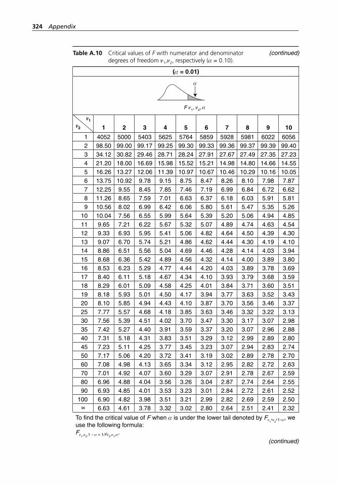
324 Appendix
Table A.10 Critical values of F with numerator and denominator degrees of freedom ν1,ν2, respectively (α = 0.10).
(α = 0.01)
F 1, 2,
m1
m2 1 2 3 4 5 6 7 8 9 10
1 4052 5000 5403 5625 5764 5859 5928 5981 6022 60562 98.50 99.00 99.17 99.25 99.30 99.33 99.36 99.37 99.39 99.403 34.12 30.82 29.46 28.71 28.24 27.91 27.67 27.49 27.35 27.234 21.20 18.00 16.69 15.98 15.52 15.21 14.98 14.80 14.66 14.555 16.26 13.27 12.06 11.39 10.97 10.67 10.46 10.29 10.16 10.056 13.75 10.92 9.78 9.15 8.75 8.47 8.26 8.10 7.98 7.877 12.25 9.55 8.45 7.85 7.46 7.19 6.99 6.84 6.72 6.628 11.26 8.65 7.59 7.01 6.63 6.37 6.18 6.03 5.91 5.819 10.56 8.02 6.99 6.42 6.06 5.80 5.61 5.47 5.35 5.26
10 10.04 7.56 6.55 5.99 5.64 5.39 5.20 5.06 4.94 4.8511 9.65 7.21 6.22 5.67 5.32 5.07 4.89 4.74 4.63 4.5412 9.33 6.93 5.95 5.41 5.06 4.82 4.64 4.50 4.39 4.3013 9.07 6.70 5.74 5.21 4.86 4.62 4.44 4.30 4.19 4.1014 8.86 6.51 5.56 5.04 4.69 4.46 4.28 4.14 4.03 3.9415 8.68 6.36 5.42 4.89 4.56 4.32 4.14 4.00 3.89 3.8016 8.53 6.23 5.29 4.77 4.44 4.20 4.03 3.89 3.78 3.6917 8.40 6.11 5.18 4.67 4.34 4.10 3.93 3.79 3.68 3.5918 8.29 6.01 5.09 4.58 4.25 4.01 3.84 3.71 3.60 3.5119 8.18 5.93 5.01 4.50 4.17 3.94 3.77 3.63 3.52 3.4320 8.10 5.85 4.94 4.43 4.10 3.87 3.70 3.56 3.46 3.3725 7.77 5.57 4.68 4.18 3.85 3.63 3.46 3.32 3.22 3.1330 7.56 5.39 4.51 4.02 3.70 3.47 3.30 3.17 3.07 2.9835 7.42 5.27 4.40 3.91 3.59 3.37 3.20 3.07 2.96 2.8840 7.31 5.18 4.31 3.83 3.51 3.29 3.12 2.99 2.89 2.8045 7.23 5.11 4.25 3.77 3.45 3.23 3.07 2.94 2.83 2.7450 7.17 5.06 4.20 3.72 3.41 3.19 3.02 2.89 2.78 2.7060 7.08 4.98 4.13 3.65 3.34 3.12 2.95 2.82 2.72 2.6370 7.01 4.92 4.07 3.60 3.29 3.07 2.91 2.78 2.67 2.5980 6.96 4.88 4.04 3.56 3.26 3.04 2.87 2.74 2.64 2.5590 6.93 4.85 4.01 3.53 3.23 3.01 2.84 2.72 2.61 2.52
100 6.90 4.82 3.98 3.51 3.21 2.99 2.82 2.69 2.59 2.50∞ 6.63 4.61 3.78 3.32 3.02 2.80 2.64 2.51 2.41 2.32
To find the critical value of F when α is under the lower tail denoted by Fν1,ν2
,1–α, we use the following formula:Fν1,ν2,1 – α = 1/Fν2,ν1,α
.
(continued)
(continued)
H1277 ch12 App.indd 324H1277 ch12 App.indd 324 3/8/07 12:57:20 PM3/8/07 12:57:20 PM
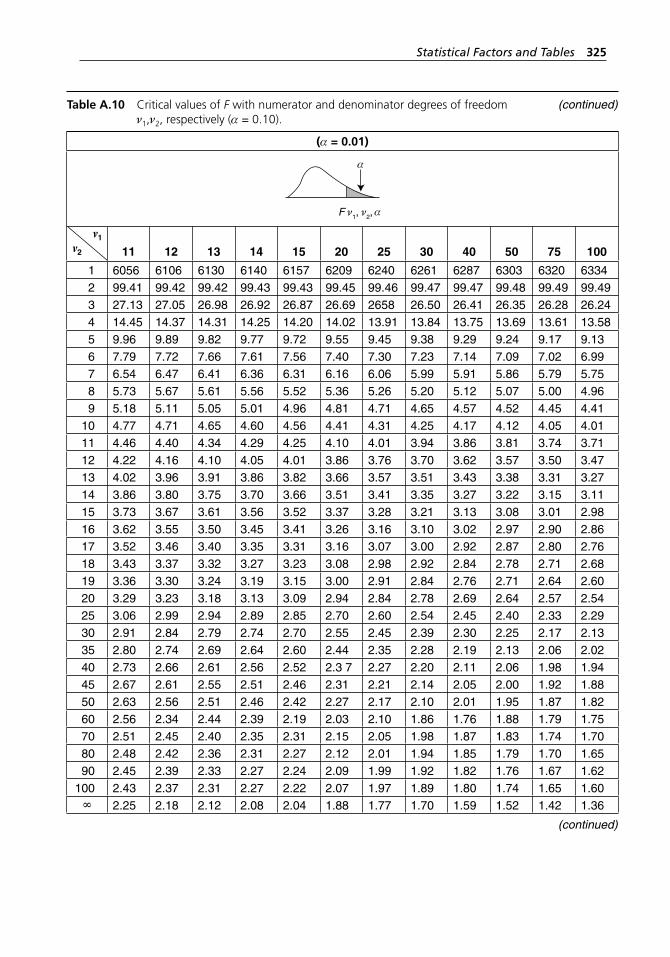
Statistical Factors and Tables 325
Table A.10 Critical values of F with numerator and denominator degrees of freedom ν1,ν2, respectively (α = 0.10).
(α = 0.01)
F 1, 2,
m1
m2 11 12 13 14 15 20 25 30 40 50 75 100
1 6056 6106 6130 6140 6157 6209 6240 6261 6287 6303 6320 63342 99.41 99.42 99.42 99.43 99.43 99.45 99.46 99.47 99.47 99.48 99.49 99.493 27.13 27.05 26.98 26.92 26.87 26.69 2658 26.50 26.41 26.35 26.28 26.244 14.45 14.37 14.31 14.25 14.20 14.02 13.91 13.84 13.75 13.69 13.61 13.585 9.96 9.89 9.82 9.77 9.72 9.55 9.45 9.38 9.29 9.24 9.17 9.136 7.79 7.72 7.66 7.61 7.56 7.40 7.30 7.23 7.14 7.09 7.02 6.997 6.54 6.47 6.41 6.36 6.31 6.16 6.06 5.99 5.91 5.86 5.79 5.758 5.73 5.67 5.61 5.56 5.52 5.36 5.26 5.20 5.12 5.07 5.00 4.969 5.18 5.11 5.05 5.01 4.96 4.81 4.71 4.65 4.57 4.52 4.45 4.41
10 4.77 4.71 4.65 4.60 4.56 4.41 4.31 4.25 4.17 4.12 4.05 4.0111 4.46 4.40 4.34 4.29 4.25 4.10 4.01 3.94 3.86 3.81 3.74 3.7112 4.22 4.16 4.10 4.05 4.01 3.86 3.76 3.70 3.62 3.57 3.50 3.4713 4.02 3.96 3.91 3.86 3.82 3.66 3.57 3.51 3.43 3.38 3.31 3.2714 3.86 3.80 3.75 3.70 3.66 3.51 3.41 3.35 3.27 3.22 3.15 3.1115 3.73 3.67 3.61 3.56 3.52 3.37 3.28 3.21 3.13 3.08 3.01 2.9816 3.62 3.55 3.50 3.45 3.41 3.26 3.16 3.10 3.02 2.97 2.90 2.8617 3.52 3.46 3.40 3.35 3.31 3.16 3.07 3.00 2.92 2.87 2.80 2.7618 3.43 3.37 3.32 3.27 3.23 3.08 2.98 2.92 2.84 2.78 2.71 2.6819 3.36 3.30 3.24 3.19 3.15 3.00 2.91 2.84 2.76 2.71 2.64 2.6020 3.29 3.23 3.18 3.13 3.09 2.94 2.84 2.78 2.69 2.64 2.57 2.5425 3.06 2.99 2.94 2.89 2.85 2.70 2.60 2.54 2.45 2.40 2.33 2.2930 2.91 2.84 2.79 2.74 2.70 2.55 2.45 2.39 2.30 2.25 2.17 2.1335 2.80 2.74 2.69 2.64 2.60 2.44 2.35 2.28 2.19 2.13 2.06 2.0240 2.73 2.66 2.61 2.56 2.52 2.3 7 2.27 2.20 2.11 2.06 1.98 1.9445 2.67 2.61 2.55 2.51 2.46 2.31 2.21 2.14 2.05 2.00 1.92 1.8850 2.63 2.56 2.51 2.46 2.42 2.27 2.17 2.10 2.01 1.95 1.87 1.8260 2.56 2.34 2.44 2.39 2.19 2.03 2.10 1.86 1.76 1.88 1.79 1.7570 2.51 2.45 2.40 2.35 2.31 2.15 2.05 1.98 1.87 1.83 1.74 1.7080 2.48 2.42 2.36 2.31 2.27 2.12 2.01 1.94 1.85 1.79 1.70 1.6590 2.45 2.39 2.33 2.27 2.24 2.09 1.99 1.92 1.82 1.76 1.67 1.62
100 2.43 2.37 2.31 2.27 2.22 2.07 1.97 1.89 1.80 1.74 1.65 1.60∞ 2.25 2.18 2.12 2.08 2.04 1.88 1.77 1.70 1.59 1.52 1.42 1.36
(continued)
(continued)
H1277 ch12 App.indd 325H1277 ch12 App.indd 325 3/8/07 12:57:21 PM3/8/07 12:57:21 PM

H1277 ch12 App.indd 326H1277 ch12 App.indd 326 3/8/07 12:57:21 PM3/8/07 12:57:21 PM

327
ANSI/ASQ. 2003. ANSI/ASQ Z1.4-2003: Sampling Procedures and Tables for Inspection by Attributes. Milwaukee, WI: ASQ Quality Press.
———. 2003. ANSI/ASQ Z1.9-2003: Sampling Procedures and Tables for Inspection by Variables for Percent Nonconforming. Milwaukee, WI: ASQ Quality Press.
Automotive Industry Action Group (AIAG) and Measurement Systems Anal-ysis (MSA) Work Group. 2002. Measurement Systems Analysis Refer-ence Manual. 3rd ed. Dearborn, MI: Automotive Industry Action Group Press.
Barrentine, L. 2003. Concepts for R&R Studies. 2nd ed. Milwaukee, WI: ASQ Quality Press.
Berger, R., D. Benbow, A. Elshennawy, and H. F. Walker. 2007. The Certi-fied Quality Engineer Handbook. 2nd ed. Milwaukee, WI: ASQ Quality Press.
Bothe, D. R. 2002. Discussion paper. Journal of Quality Technology 34 (1): 32–37.
Boyles, R. A. 1991. “The Taguchi Capability Index.” Journal of Quality Tech-nology 23 (1): 17–26.
Brown, N. 1966. “Zero Defects the Easy Way with Target Area Control.” Modern Machine Shop, 96–100.
Champ, C. M., and W. H. Woodall. 1987. “Exact Results for Shewhart Control Charts with Supplementary Run Rules.” Technometrics 29 (4): 393–399.
Chan, L. K., S. W. Cheng, and F. A. Spring. 1988. “A New Measure of Pro-cess Capability: Cpm.” Journal of Quality Technology 20:162–175.
Chen, S. M., and N. F. Hsu. 1995. “The Asymptotic Distribution of the Process Capability Index Cpmk.” Commun. Statist.-Theory and Method 24 (5): 1279–1291.
Cochran, W. G. 1977. Sampling Techniques. 3rd ed. New York: John Wiley & Sons.
Crowder, S. V. 1987. “Computation of ARL for Combined Individual Mea-surements and Moving Range Charts.” Journal of Quality Technology 19 (1): 98–102.
Bibliography
H1277 ch13_BIB.indd 327H1277 ch13_BIB.indd 327 3/8/07 12:57:48 PM3/8/07 12:57:48 PM
328 Bibliography
———. 1989. “Design of Exponentially Weighted Moving Average Schemes.” Journal of Quality Technology 21 (2): 155–162.
Deleryd, M. 1996. “Process Capability Studies in Theory and Practice.” Licentiate thesis, Lulea University of Technology, Lulea, Sweden.
Deming, W. E. 1950. Some Theory of Sampling. New York: John Wiley & Sons.
———. 1951. Elementary Principles of the Statistical Control of Quality. 2nd ed. Tokyo: Nippon Kagaku Gijutsu Remmei.
———. 1975. “On Some Statistical Aids toward Economic Production.” Interfaces 5 (4): 5.
———. 1982. Quality, Productivity, and Competitive Position. Cambridge, MA: MIT, Center for Advanced Engineering Study.
———. 1986. Out of the Crisis. Boston, MA: MIT, Center for Advanced Engineering Study.
Duncan, A. J. 1986. Quality Control and Industrial Statistics. 5th ed. Home-wood, IL: Irwin.
Ford Motor Company. 1984. Continuing Process Control and Process Capa-bility Improvement, Dearborn, MI.
Govindarajulu, Z. 1999. Elements of Sampling Theory and Methods. Upper Saddle River, NJ: Prentice Hall.
Gryna, F. M., R.C.H. Chua, and J. A. DeFeo. 2007. Jurans Quality Plan-ning & Analysis for Enterprise Quality. 5th ed. New York: McGraw- Hill Publishing.
Gupta, B. C. 2005. “A New Process Capability Index Cpnst.” Journal of Com-binatorics, Information & System Sciences 30:67–79.
Gupta, B. C., and C. Peng. 2004. “On the Distributional and Inferential Char-acterization of the Process Capability Index Cpnst.” Journal of Statistics and Applications 1 (1): 63–72.
Gupta, B. C., and F. H. Walker. 2005. Applied Statistics for the Six Sigma Green Belt. Milwaukee, WI: ASQ Quality Press.
Hawkins, D. M. 1981. “A CUSUM for a Scale Parameter.” Journal of Quality Technology 13 (4): 228–231.
———. 1993. “Cumulative Sum Control Charting, an Underutilized SPC Tool.” Quality Engineering 5 (3): 463–477.
Hawkins, D. M., and D. H. Olwell. 1998. Cumulative Sum Charts and Chart-ing for Quality Improvement. New York: Springer-Verlag.
Hsiang, T. C., and G. Taguchi. 1985. “A Tutorial on Quality Control and Assurance—The Taguchi Methods.” ASA annual meeting, Las Vegas, NV.
IBM (International Business Machines Corporation). 1984. Process Control, Capability and Improvement. Thornwood, NY: The Quality Institute.
Juran, J., and A. B. Godfrey. 1999. Juran’s Quality Handbook. 5th ed. New York: McGraw- Hill Publishing.
Juran, J. M., F. M. Gryna, and R. S. Bingham Jr. 1974. Quality Control Hand-book. New York: McGraw- Hill.
Kane, V. E. 1986. “Process Capability Indices.” Journal of Quality Technol-ogy 18:41–52.
H1277 ch13_BIB.indd 328H1277 ch13_BIB.indd 328 3/8/07 12:57:48 PM3/8/07 12:57:48 PM
Bibliography 329
Kotz, S., and C. R. Lovelace. 1998. Process Capability Indices in Theory and Practice. London and New York: Arnold.
Ledolter, J., and A. Swersey. 1997. “An Evaluation of PRE- Control.” Journal of Quality Technology 29 (2): 163–171.
Lohr, S. L. 1999. Sampling: Design and Analysis. Pacific Grove, CA: Dux-bury Press.
Lucas, J. M. 1982. “Combined Shewhart- CUSUM Quality Control Schemes.” Journal of Quality Technology 14 (2): 51–59.
Lucas, J. M., and R. B. Crosier. 1982. “Fast Initial Response for CUSUM Quality Control Schemes.” Technometrics 24 (3): 199–205.
Lucas, J. M., and M. S. Saccucci. 1990. “Exponentially Weighted Moving Average Control Schemes: Properties and Enhancements.” Technometrics 32 (1): 1–29.
Montgomery, D. C. 2005a. Design and Analysis of Experiments. 6th ed. New York: John Wiley & Sons.
———. 2005b. Introduction to Statistical Quality Control. 5th ed. New York: John Wiley & Sons.
Ott, E., E. Schilling, and D. Neubauer. 2005. Process Quality Control: Trou-bleshooting and Interpretation of Data. 4th ed. Milwaukee, WI: ASQ Quality Press.
Pearn, W. L., and S. Kotz. 1994. “Application Element’s Method for Calcu-lating Second and Third Generation Process Capability Indices for Non- normal Pearsonian Populations.” Quality Engineering 7 (1): 139–145.
Pearn, W. L., S. Kotz, and N. L. Johnson. 1992. “Distributional and Inferen-tial Properties of Process Capability Indices.” Journal of Quality Technol-ogy 24:216–231.
Quesenberry, C. P. 1997. SPC Methods for Quality Improvement. New York: John Wiley and Sons.
Roberts, S. W. 1959. “Control Chart Tests Based on Geometric Moving Aver-ages.” Technometrics 1 (3): 239–250.
Ryan, T. P. 2000. Statistical Methods for Quality Improvement. 2nd ed. New York: John Wiley & Sons.
Scheaffer, R. L., et al. 2006. Elementary Survey Sampling. 6th ed. Belmont, CA: Duxbury Press.
Schilling, E. G. 1982. Acceptance Sampling in Quality Control. New York:Marcel Dekker.
Shainin, D. 1984. “Better Than Good Old X-Bar and R Charts.” In ASQC Quality Congress Transactions, 302–307. Milwaukee, WI: ASQC Qual-ity Press.
Shewhart, W. A. 1980. Economic Control of Quality of Manufactured Prod-uct. New York: D. Van Nostrand Company.
Smith, G. 1991. Statistical Process Control and Quality Improvement. New York: Macmillan Publishing.
Spiring, F. A. 1997. “A Unifying Approach to Process Capability Indices.” Journal of Quality Technology 29 (1): 49–58.
Stephens, K. S. 2001. The Handbook of Applied Acceptance Sampling Plans, Procedures and Principles. Milwaukee, WI: ASQ Quality Press.
H1277 ch13_BIB.indd 329H1277 ch13_BIB.indd 329 3/8/07 12:57:48 PM3/8/07 12:57:48 PM

330 Bibliography
Taguchi, G. 1986. Introduction to Quality Engineering. Tokyo: Asian Pro-ductivity Organization.
Traver, R. 1985. “Pre-Control: A Good Alternative to X-Bar–R Charts.” ASQC Quality Progress, September, 11–14.
Urdhwareshee, H. 2006. “The Power of Pre- Control.” http://www.sympho-nytech.com/articles/precontrol.htm.
Van Dobben de Bruyn, C. S. 1968. “Cumulative Sum Tests.” In Theory and Practice. London: Griffin.
Vännman, K. 1995. “A Unified Approach to Capability Indices.” Statistica Sinica 5:805–820.
Wallgren, E. 1996. “Properties of the Taguchi Capability Index for Markov Dependent Quality Characteristic.” University of Oreboro, Sweden.
Wescott, R. 2007. The Certified Manager of Quality/Organizational Excel-lence Handbook. 3rd ed. Milwaukee, WI: ASQ Quality Press.
Western Electric. 1956. Statistical Quality Control Handbook. Indianapolis, IN: Western Electric Corporation.
Wheeler, D., and D. Chambers. 1992. Understanding Statistical Process Control. 2nd ed. Knoxville, TN: SPC Press.
Wheeler, D., and R. Lyday. 1989. Evaluating the Measurement Process. 2nd ed. Knoxville, TN: SPC Press.
H1277 ch13_BIB.indd 330H1277 ch13_BIB.indd 330 3/8/07 12:57:48 PM3/8/07 12:57:48 PM
331
Page numbers followed by f or t refer to figures or tables, respectively.
A
acceptable quality limit (AQL), 178, 194acceptance number, sampling plans
and, 180–182acceptance sampling, 2. See also
samplingby attributes, 177double sampling plans, 184intent of, 173–174multiple sampling plans, 186standards, 188–193switching procedures, 190–191, 190fby variables, 193–194
accuracy, vs. precision, 151, 151faccuracy of measurement system,
defined, 151action on output, 51–52action on process, 51actions on system, for variation, 53alpha (α) risk, 7–9ANOVA, MSA based on, 156–162ANSI/ASQ Z1.4-2003, 188–189, 205f,
206f, 207f, 208f, 209–210flevels of inspection in, 189–191types of sampling and, 191–193
ANSI/ASQ Z1.9-2003, 194–198, 211f, 212f, 213–221f, 222f
AQL levels in, 195Form 1 for, 195
Form 2 for, 195structure and organization of,
195fAOQ. See average outgoing quality
(AOQ)AOQL. See average outgoing quality
limit (AOQL)applied statistics, SQC and, 2–3, 3fAQL. See acceptable quality limit
(AQL)ARL. See average run length
(ARL)ASN. See average sample number
(ASN)assignable causes, of variation. See
special causes, of variationasymptotically normal, 139attributes
acceptance sampling by, 177control charts for, 83–84, 85t
c charts, 93–96np charts, 92–93p charts, 85–90u charts, 96–100
defined, 83attribute sampling plans. See also
sampling plansANSI/ASQ Z1.4-2003 and, 189double, 184–185multiple, 186single, 182–184vs. variables sampling plans,
193–194
Index
H1277 ch14_IDX.indd 331H1277 ch14_IDX.indd 331 3/8/07 1:37:58 PM3/8/07 1:37:58 PM
332 Index
average outgoing quality (AOQ), 178–179
for double/multiple sampling plans, 186
average outgoing quality limit (AOQL), 179–180
for double/multiple sampling plans, 186
average quality protection, 175average run length (ARL), 57–58
of two-sided control chart, 106average sample number (ASN),
186–188
B
bad decisions, risk associated with making, 7–9
beta (β) risk, 7–9binomial distribution, 85, 86, 175, 176
C
calibration, 45, 60capability analysis, 2cause-and-effect diagram, 43, 47–48, 48fc control charts, 93–96
JMP for creating, 282–283MINITAB for, 240
center line (CL), for control charts, 54central limit theorem (CLT), 148, 148fcheck sheets, 43–45, 44fcluster random sampling, 15, 32–37.
See also samplingadvantages of, 33confidence interval for population
mean for, 34–37confidence interval for population
total for, 34–37determination of sample size for, 37estimation of population mean for,
33–34estimation of population total for,
33–34one-stage, 33two-stage, 33
combined Shewhart-CUSUM control charts, 115–116
common causes, of variation, 52confidence coefficients, 15confidence intervals, 15conforming, use of term, 83consumer risk, 178
defined, 8continuous sampling plans, 201
types of, 201–203control charts, 43, 54f
action on output for, 51–52action on process for, 51for attributes, 83–84, 85t
c charts, 93–96np charts, 92–93p charts, 85–90u charts, 96–100
benefits of, 56center line for, 54exponentially weighted moving
average (see exponentially weighted moving average (EWMA) control charts)
lower control limit for, 54moving average (see moving average
(MA) control charts)preparation for use of, 55–56process evaluation for, 51rational samples for, 57for separating separate causes from
common causes, 53Shewhart (see Shewhart control
charts)upper control limit for, 54uses of, 54variation and, 52–53
control limits (CL)calculation of, for Shewhart X bar
and R control charts, 61–64calculation of, for Shewhart X bar
and S control charts, 73–75for np control charts, 92–93
correlation between characteristics, determining, 55
critical defects, 189
H1277 ch14_IDX.indd 332H1277 ch14_IDX.indd 332 3/8/07 1:37:59 PM3/8/07 1:37:59 PM
Index 333
cumulative sum (CUSUM) control charts, 101–102. See also combined Shewhart-CUSUM control charts
basic assumptions of, 102for controlling process variability,
116–117designing, 104–106detecting small shifts and, 101FIR feature for, 112–115, 245JMP for creating, 286–288MINITAB for, 243–245one-sided, 104–106, 115two-sided, 104–106two-sided, using numerical
procedure, 106–112vs. Shewhart X bar-R control charts,
102–104, 105fCUSUM control charts. See
cumulative sum (CUSUM) control charts
D
decision making, on quantitative data, 5
defect concentration diagram, 43, 48–49, 49f
defect rate, 167defects
critical, 189major, 189minor, 189
Deming, W. Edwards, 39–40design of experiments (DOE), SQC
and, 2–3distinct categories, determining
number of, 158–159Dodge-Romig tables, 193Dodge’s continuous sampling plans,
201–202double sampling, 191–192,
193fdouble sampling plans
AOQ curve for, 186AOQL for, 186
double, 184OC curve for, 184–185
downward shift, 102, 106, 115, 243, 286
E
Economic Control of Quality of Manufactured Product (Shewhart), 39
environmentas a category in a cause-and-effect
diagram, 48, 48f, 49fas cause of part-to-part variation,
149as part of a process, 41, 55, 127in preparing control charts, 55
error of estimation, 15estimate, 15estimator, 15EWMA control charts. See
exponentially weighted moving average (EWMA) control charts
exponentially weighted moving average (EWMA) control charts, 101–102, 120–125
JMP for creating, 290–292MINITAB for, 247–249
F
fast initial response (FIR) feature, for CUSUM control charts, 112–115, 245
fieldworkers, 13finite populations, 12FIR feature. See fast initial response
(FIR) feature, for CUSUM control charts
fishbone. See cause-and-effect diagram
Form 1, for ANSI/ASQ Z1.9-2003, 195
Form 2, for ANSI/ASQ Z1.9-2003, 195
H1277 ch14_IDX.indd 333H1277 ch14_IDX.indd 333 3/8/07 1:37:59 PM3/8/07 1:37:59 PM
334 Index
G
Gage repeatability and reproducibility (Gage R&R) study, 147. See also measurement system analysis (MSA); measurement system performance
ANOVA method for, 156–159graphical representation of, 159–162,
256–259JMP for, 293–298, 295f, 296f, 297f,
298fMINITAB for, 250–259total, 152
geometric series, 121–122
H
histograms, 43
I
individual observations, Shewhart control charts for, 69
infinite populations, 12inspection
levels of, 189–191sampling vs. 100 percent, 174–175
interaction between instruments and operators, 149, 152
Ishikawa diagram. See cause-and-effect diagram
J
JMP software packagefor capability analysis, 275–277for creating c control charts,
282–283, 282f, 283ffor creating CUSUM control charts,
286–288, 287f, 288ffor creating EWMA control charts,
290–292, 291f, 292fcreating new data table for, 264–265for creating p control charts,
277–281, 280ffor creating u control charts,
284–286, 284f, 285f
for creating UWMA chart, 288–290, 289f, 290f
for Gage R&R study, 293–298getting started with, 263–264for measurement system capability
analysis, 292–298, 295f, 296f, 297f, 298f
normal quantile plot, 279fopening existing files, 265print options, 266for process capability analysis,
275–277, 278f, 279fsaving files, 265–266Starter, 261–262for Shewhart control chart for
individual observations, 273–275
for Shewhart Xbar and R control charts, 268–270
for Shewhart Xbar and S control charts
with equal sample size, 270–272with sample size variable,
272–273using, 261–263using images for reporting, 267–268
L
linearity, 151, 151fline graphs. See run chartslocal actions, for variation, 53lot-by-lot sampling, 175lot size, sampling plans and,
180–182lot tolerance percent defective (LTPD),
178lower control limit (LCL), for control
charts, 54LTPD. See lot tolerance percent
defective (LTPD)
M
MA control charts. See moving average (MA) control charts
major defects, 189margin of error, 15
H1277 ch14_IDX.indd 334H1277 ch14_IDX.indd 334 3/8/07 1:37:59 PM3/8/07 1:37:59 PM
Index 335
MCI. See measurement capability index (MCI)
measurementdefined, 147volume of operations and, 7
measurement capability index (MCI), 150, 162
as percentage of process specification, 163
as percentage of process variation, 162–163
measurement system, defined, 147measurement system analysis (MSA),
147based on ANOVA, 156–162based on range, 150–156
measurement system capability analysis
computer resources for, 249–259JMP for, 292–298, 295f, 296f, 297f,
298fMINITAB for, 249–259
measurement system performance, evaluating, 149–162. See also Gage repeatability and reproducibility (Gage R&R) study
measurement system variation, 249, 292–293
MIL-STD-1235B, 202–203MINITAB
for c control charts, 240creating new worksheet, 226–227for CUSUM control charts,
243–245for EWMA control charts, 247–249getting starting with, 226for MA control charts, 245–247for measurement system capability
analysis, 249–259for np control charts, 239for p control charts, 238–239print options for, 228for process capability analysis,
235–237retrieving saved MINITAB data file,
227saving data file, 227
saving project, 227–228for Shewhart control chart for
individual observations, 230–231
for Shewhart Xbar and R control charts, 228–229
for Shewhart Xbar and S control charts
equal sample size, 231–233sample size variable, 233–235
for u control charts, 241–243using, 225–226
minor defects, 189moving average (MA) control charts,
101–102, 117–120MINITAB for, 245–247
moving range (MR), 69MSA. See measurement system
analysis (MSA)multiple sampling, 191–192, 193fmultiple sampling plans, 186
AOQ curve for, 186AOQL for, 186
N
near zero, 167nonconforming, use of term, 83normal inspection to reduced
inspection, 190–191normal inspection to tightened
inspection, 190np control charts, 92–93
JMP for creating, 281MINITAB for, 239
O
OC curve. See operating characteristic (OC) curve
100 percent inspection, 174–175one-sided CUSUM control charts,
104–106, 115one-stage cluster random sampling, 33operating characteristic (OC) curve,
57, 59–60, 175–176for double sampling plans, 184–185plotting, 176–177
H1277 ch14_IDX.indd 335H1277 ch14_IDX.indd 335 3/8/07 1:37:59 PM3/8/07 1:37:59 PM
336 Index
P
Pareto charts, 43, 45–46, 45f, 47fpart-to-part variation, 149, 249,
292–293patterns
of defects, 45, 48–49of nonrandomness, 64, 66presence of unusual, 87of random variation, 54, 55using run charts to identify, 50–51,Western Electric criteria, 64
p control charts, 85–90control chart for fraction
nonconforming with variable samples, 89–90
control limits for, 85–87interpreting, for fraction
nonconforming, 87–89JMP for creating, 277–281, 280fMINITAB for, 238–239
point estimate. See estimatePoisson distribution, 94, 175, 176population, sampled, 13population mean, confidence interval
for, 20for cluster random sampling, 34–37for simple random sampling, 20for systematic random sampling, 30
population mean, estimation of, 16–19
for cluster random sampling, 33–34for simple random sampling, 16–19for stratified random sampling,
22–24for systematic random sampling,
28–30populations
defined, 12finite, 12infinite, 12target, 12
population totalconfidence interval for, 20
for cluster random sampling, 34–37for simple random sampling, 20for systematic random sampling, 30
estimation of, 16–19for cluster random sampling, 33–34for simple random sampling, 16–19for stratified random sampling,
22–24for systematic random sampling,
28–30practical versus theoretical difference,
5–6precision, vs. accuracy, 151, 151fPRE-control, 2
advantages of, 170–171background of, 165–166color-coding scheme for, 167–168disadvantages of, 171–172goals of, 166mechanics of, 168–169necessary conditions for valid,
166–167statistical basis for, 170
pretests, 13probability, defined, 8process
defined, 1, 41flowchart of, 41fvariation and, 52
process capability, 79–81, 80fprocess capability analysis, 128–129
implementing, 129JMP for creating, 275–277MINITAB for, 235–237ways of using results of, 129
process capability indices (PCIs), 127–145, 166
Cp, 130–134Cpk, 135–136Cpm, 136–138Cpmk, 138–139Cpnst, 139–144defined, 128development of, 127–130first-generation, 130flowchart of, 128fPp and Ppk, 144–145
process evaluation, 1process Six Sigma, order of topics in,
3–4, 4f
H1277 ch14_IDX.indd 336H1277 ch14_IDX.indd 336 3/8/07 1:37:59 PM3/8/07 1:37:59 PM
Index 337
process variability, CUSUM control charts for controlling, 116–117
producer risk, 178defined, 8
Q
qualitative data, defined, 5quality
benefits of better, 40–41defined, 40
quality characteristics, 7, 56, 79, 83behavior of, 42examples of attributes, 84reducing variation of, 43using a p chart to study, 85
quality control charts, 39, 42categories of, 42
quantitative data, decision-making and, 5
R
random causes. See common causes, of variation
range method, 150rational samples, for control charts,
57reduced inspection to normal
inspection, 191repeatability, 149
defined, 150–151, 152–153reproducibility, 149
defined, 151, 153risks
bad decisions and, 7–9consumer, 8, 178producer, 8, 178
run, defined, 57run charts, 43, 49f, 50–51
S
sample, defined, 12sample designs, 11
cluster random sampling, 15simple random sampling, 13
stratified random sampling, 13, 14systematic random sampling, 13, 14
sampled population, defined, 13sample mean, defined, 17samples, 5f, 7
determining size of, 57–60sample size
average run length and, 57–58determination of, 20–21
average run length for, 57–58for cluster random sampling, 37operating characteristic curve for,
57, 59–60for simple random sampling, 20–21for stratified random sampling,
26–27for systematic random sampling,
30–32operating characteristic curve and,
57, 59–60sampling plans and, 180–182variable, for Shewhart X bar and S
control charts, 76–79sample statistics, calculation of, for
Shewhart X bar and R control charts, 60–61
sample variance, defined, 17sampling
acceptance (see acceptance sampling)
advantages of, 174basic concepts of, 11–15cluster random (see cluster random
sampling)concepts of, 175–182double, 191–192, 193fmultiple, 191–192, 193fsimple random (see simple random
sampling)single, 191–192, 193fstandards, 188–193stratified random (see stratified
random sampling)systematic random (see systematic
random sampling)types of, ASI/ASQ Z1.4-2003 and,
191–193
H1277 ch14_IDX.indd 337H1277 ch14_IDX.indd 337 3/8/07 1:37:59 PM3/8/07 1:37:59 PM
338 Index
sampling frame, defined, 13sampling inspection, 174–175sampling plans. See also attribute
sampling plansacceptance number and, 180–182continuous, 201–203lot size and, 180–182sample size and, 180–182sequential, 199–201standards for, 188–193variables, 193–198
scatter diagram, 43sequential sampling plans, 199–201
decision areas for, 199fShainin, Dorian, 165Shewhart, Walter A., 39, 42Shewhart control charts. See also
combined Shewhart-CUSUM control charts
for individual observations, MINITAB for, 230–231
individual observations for, 69–72Shewhart Xbar and R control charts
calculation of control limits for, 61–64
calculation of sample statistics for, 60–61
constructing, with known process mean and process standard deviation, 230
constructing, with MINITAB, 228–229
extending current control limits for future control for, 66–68
interpretation of, 64–66JMP software package for, 268–270rules for preparing, 60vs. CUSUM control charts, 102–104when process mean and process
standard deviation are known, 68–69
Shewhart Xbar and S control chartscalculation of control limits for,
73–75constructing, with MINITAB
for equal sample size, 231–233for variable sample size, 233–235
vs. R charts, 72–73when sample size is variable, 76–79
simple random sample, defined, 15–16simple random sampling, 13, 14,
15–21. See also samplingconfidence interval for population
mean for, 20confidence interval for population
total for, 20determination of sample size for,
20–21estimation of population mean for,
16–19estimation of population total for,
16–19single sampling plans, 182–184,
191–192, 193fSix Sigma
order of topics in process of, 3transactional, 3–4, 4f
Six Sigma Green Belt, statistical quality control and, 1
SPC. See statistical process control (SPC)
special causes, of variation, 52SQC. See statistical quality control
(SQC)stability, defined, 151stable process, 79standard normal distribution, 167,
170statistical control, defined, 166statistical process control (SPC), 1–2,
41–51tools of, 43–51
statistical quality control (SQC), 2applied statistics and, 2–4defined, 1design of experiments and, 2–4relationships among tools of, 165frole of statistics in, 4–5Six Sigma Green Belt and, 1tool types of, 2, 2funderstanding variability with,
148–149use of modern, 39
statistical significance, 5–6
H1277 ch14_IDX.indd 338H1277 ch14_IDX.indd 338 3/8/07 1:37:59 PM3/8/07 1:37:59 PM
Index 339
statisticsapplied, SQC and, 2–4role of, in SQC, 4–5
stem-and-leaf diagram, 43stratified random sampling, 13, 14,
21–27. See also sampling; stratified random sampling
advantages of, 21–22confidence interval for population
mean for, 24–27confidence interval for population
total for, 24–27determination of sample size for,
26–27estimation of population mean for,
22–24estimation of population total for,
22–24process of, 22
systematic random sampling, 13, 14, 27–32
advantages of, 27–28confidence interval for population
mean for, 30confidence interval for population
total for, 30determination of sample size for,
30–32estimation of population mean for,
28–30estimation of population total for,
28–30
T
target populations, 12test significance (α), level of, 5–6tightened inspection to normal
inspection, 190time series graphs. See run chartstotal Gage R&R variability, 152total process variation, 149. See also
variationmeasurement system variation, 249part-to-part variation source, 249
total variability, components of, 151–152
transactional Six Sigma, order of topics in, 3–4, 4f
two-sided CUSUM control charts, 104–106
using numerical procedure, 106–112two-stage cluster random sampling, 33Type I error, 7–9Type II error, 7–9
U
u control charts, 96–100JMP for creating, 284–286MINITAB for, 241–243
uniformly weighted moving average (UWMA) chart, JMP for creating, 288–290
upper control line (UCL), for control charts, 54
upward shift, 102, 106, 115, 243, 286UWMA. See uniformly weighted
moving average (UWMA) chart, JMP for creating
V
variabilityin measurement process, 148–149in production/service delivery
process, 148total, components of, 151–152
variable, defined, 42variables sampling plans, 193–198
ANSI/ASQ Z1.9-2003 and, 194–198benefits of, over attribute plans,
193–194when standard deviation is known,
203–204variation. See also total process
variationactions on system for, 53causes of, 42, 127common causes of, 52controlling, 42defined, 42due to measurement instruments, 149due to operators, 149
H1277 ch14_IDX.indd 339H1277 ch14_IDX.indd 339 3/8/07 1:37:59 PM3/8/07 1:37:59 PM

340 Index
local actions for, 53minimizing unnecessary, 56part-to-part, 149special causes of, 52
vendor certification, 174vendor qualification, 174V-mask, 106, 244
W
Western Electric criteriafor detecting small shifts, 101–102for determining nonrandom patterns
on control charts, 64
H1277 ch14_IDX.indd 340H1277 ch14_IDX.indd 340 3/8/07 1:37:59 PM3/8/07 1:37:59 PM