Transactions of the ASABE

Vol. 51(2): 413-424 � 2008 American Society of Agricultural and Biological Engineers ISSN 0001-2351 413

SITE‐SPECIFIC DECISION‐MAKING BASED ON RTK GPSSURVEY AND SIX ALTERNATIVE ELEVATION DATA SOURCES:

SOIL EROSION PREDICTIONS

C. S. Renschler, D. C. Flanagan

ABSTRACT. Precision farming equipment based on Global Positioning Systems (GPS) enables landowners to gather spatiallydistributed topographic data in real‐time kinematic (RTK) mode, which has the potential to be used in addition to or assubstitute for commonly available topographic data sources (e.g., U.S. Geological Survey (USGS) topographic contour linesand/or digital elevation models). The latter are considered insufficiently accurate in their topographical representation ofwatershed boundaries, slopes, and upslope contributing areas to be able to meaningfully apply detailed process‐based soilerosion assessment tools at the field scale. In this second of two articles discussing the usefulness of the available data setsfrom a decision‐maker's perspective, the same comprehensive accuracy tests that were used for these topographicalparameters are applied to the spatially distributed soil erosion assessment results simulated by the Water Erosion PredictionProject (WEPP) model supported by Geographic Information Systems (GIS). The impact of the accuracy of six alternativetopographical data sources on predicting soil erosion rates using WEPP is compared to on‐site soil erosion predictions usingelevation measurements from a survey‐grade RTK GPS with centimeter accuracy. Results show that the more precisetopographic measurements with a photogrammetric survey or any differential GPS units yield more precise on‐site soil losspredictions for individual raster cells (0.01 ha) and hillslope areas of interest (0.5 ha). However, the best WEPP predictionsfor average annual off‐site runoff (-18.3% error) and sediment yield (-2.7% error) from upslope contributing areas of about4 ha within the 30 ha watershed were achieved using the USGS 10 ft contours. These results demonstrate that in this case,the runoff and sediment yield predictions using DEMs based on the commonly available contour lines can be even better thanthose from the more precise and costly topographic data sets. The contours also allowed successful application of the WEPPmodel to identify all 11 hillslope areas of interest (0.5 ha) with soil loss (10) or deposition (1) problems that were initiallymapped in the field as larger rills and sedimentation areas, respectively.

Keywords. Accuracy, Decision‐making, Erosion, Global positioning systems, Modeling, Topography, Watershed, WEPP.

ne of the most fundamental requirements for mod‐eling landscape topography and soil erosion pro‐cesses is the accurate representation of topo-graphy. To be useful for decision‐makers, soil ero‐

sion models must have simple data requirements, must con‐sider spatial and temporal variability in hydrological and soilerosion processes, and must be applicable to a variety of re‐gions with minimum calibration (Renschler and Harbor,2002). Over the past few years, more land users have beenable to gather more accurate site‐specific information aboutsoil, vegetation, and plant residue characteristics from preci‐

Submitted for review in June 2006 as manuscript number SW 6528;approved for publication by the Soil & Water Division of ASABE inFebruary 2008.

The use of trade names does not imply endorsement by the Universityat Buffalo (SUNY) or the USDA Agricultural Research Service.

The authors are Chris S. Renschler, Associate Professor, Departmentof Geography, National Center for Geographic Information and Analysis(NCGIA), University at Buffalo - The State University of New York,Buffalo, New York; and Dennis C. Flanagan, ASABE Member Engineer,Agricultural Engineer, USDA‐ARS National Soil Erosion ResearchLaboratory, West Lafayette, Indiana. Corresponding author: Chris S.Renschler, Department of Geography, National Center for GeographicInformation and Analysis (NCGIA), University at Buffalo - The StateUniversity of New York, 116 Wilkeson Quad, Buffalo, NY 14261; phone:716‐645‐2722, ext. 23; fax: 716‐645‐2329; e‐mail: rensch@buffalo.edu.

sion farming techniques based on more accurate Global Posi‐tioning Systems (GPS) at a reasonable cost. Land users, suchas precision farmers, utilize these spatially distributed GPSdata mainly for applications such as yield monitoring andprecision application of nutrient and pest management. Be‐sides these main purposes of gathering soil and plant parame‐ters for site‐specific agricultural management support at aunique location (x and y), elevation data (z) are also recordedby a GPS data logger. However, these elevation data, whichare continuously gathered on a moving vehicle in real‐timekinematic (RTK) mode, have hardly been used in the past forbest management practices (BMPs) in soil and water con‐servation.

As Clark and Lee (1998) and Wilson et al. (1998) demon‐strated in different research projects, GPS elevation data havethe potential to be used for topographic mapping as well asfor topographic analysis such as flowpath, channel, and wa‐tershed delineation. Alternatively, geo‐referenced common‐ly available data sources such as topographical maps, soilsurveys, and rectified aerial photographs (orthophotos) areall readily available. These data sources depend on field sur‐veys at a certain point of time in the past and are designed tobe useful at the 1:24,000 scale of U.S. Geological Survey to‐pographical maps (USGS, 2006). These data sets are usuallyavailable nationwide and are provided free of charge by U.S.federal agencies (USGS, 2006; NRCS, 2006). Renschler et

O

414 TRANSACTIONS OF THE ASABE

al. (2002a) analyzed the impact of the accuracy of six alterna‐tive topographical data sources on watershed topography anddelineation in comparison to GPS measurements of a survey‐grade GPS with centimeter accuracy. The results demon‐strated that the most accurate and expensive alternativeswere most useful for determining elevation and slopes in theflow direction, while there was not much difference betweenalternative topographic data sources in obtaining upslopedrainage areas and delineation of the channel network andwatershed boundary. User‐friendly soil erosion assessmenttools such as the Geospatial Interface for the Water ErosionPrediction Project (GeoWEPP) model are capable of usingthese sources of information and precision farming data setsto support the decision‐making process for sustainable landuse and soil and water conservation (Renschler, 2003).

The Water Erosion Prediction Project (WEPP; Flanaganand Nearing, 1995; Flanagan et al., 2001) model is a physi‐cally based, continuous simulation, erosion prediction toolfor use on personal computers. It was developed through ajoint effort of several federal agencies, including the USDAAgricultural Research Service (ARS), USDA Natural Re‐sources Conservation Service (NRCS), USDA Forest Service(FS), and the USDI Bureau of Land Management (BLM), toreplace more empirically based technologies such as the Uni‐versal Soil Loss Equation (USLE; Wischmeier and Smith,1978) and RUSLE (Revised USLE; Renard et al., 1997).WEPP simulates the important physical processes related toerosion by water, including infiltration, runoff, detachmentby rainfall, detachment by flow, sediment transport, sedimentdeposition, plant growth, and residue decomposition andmanagement. The model is applicable to small watersheds(<250 ha) as well as to individual hillslope profiles (Flanaganet al., 2001).

In order to assist users with application of WEPP to smallwatersheds, interfaces between the model and GeographicInformation Systems (GIS) were created that allow use ofspatial digital elevation data for an area to be automaticallyprocessed into hillslope profile and channel input slope files(Cochrane and Flanagan, 2003), ultimately culminating intwo sets of WEPP‐GIS tools. The first was the GeoWEPPsoftware (Renschler et al., 2002b; Renschler, 2003), which isan ArcView 3.2 extension soon to migrate to be an ArcGIS9 (ESRI, 2006) extension. The second is a web‐based WEPP‐GIS interface (Flanagan et al., 2004a, 2004b) that uses theopen‐source Mapserver environment (UNM, 2006). All ofthese WEPP interfaces rely on the TOPAZ (TopographicParameterization; Garbrecht and Martz, 1997) digital land‐scape analysis tool to delineate channels, watersheds, andsub‐basins.

OBJECTIVES

The main objective of this article is to analyze the impactof the accuracy of six alternative topographical data sourceson predicting runoff and soil erosion rates using the WEPPmodel (Flanagan and Nearing, 1995). To test the applicabilityand accuracy of six alternative methods, seven data sets wereobtained for a topographic analysis, and all results werecompared to the most recently gathered and most preciseavailable data set: a highly accurate survey‐grade GPS unitin RTK mode. Instead of gathering data in optimal conditions(e.g., a sufficient number and optimum distribution of GPSsatellites in view), all the GPS data sets were collected at the

same time with a typical contour‐parallel management pat‐tern and speed within a three‐day period without any extraGPS measurements along the fields, e.g., fences, ditches, orterraces. This allows comparing equipment performance un‐der realistic farming conditions and an assessment of their fitfor use in topographic analysis and watershed delineation (fora photo of the GPS platform on an all‐terrain vehicle (ATV),refer to Renschler et al., 2002a).

While the previous companion article analyzed the effectof alternative data gathering methods solely on watershed to‐pography and delineation (Renschler et al., 2002a), this ar‐ticle evaluates the accuracy of each of the alternatives inobtaining elevation data and using their topographic parame‐ters for soil erosion prediction at three decision‐maker'sscales of interest. The areas that decision‐makers would beinterested in assessing, i.e., Total Maximum Daily Loads(TMDLs) of small watersheds and best management practic‐es (BMPs) along channels, are here referred to as “contribut‐ing areas of interest.” In this study, the latter category wouldinclude the entire watershed scale (30 ha; see W‐2 in fig. 1)and its channel contributing hillslope areas (>4 ha; approxi‐mately similar size as neighboring W‐11 in fig. 1). At a moredetailed scale, a decision‐maker may be interested in site‐specific locations to mitigate selected areas of concern, or“hillslope areas of interest” (0.5 ha), for the optimization ofBMP locations. The most detailed resolution possible, buthardly considered by a decision‐maker for making anylocation‐based land cover change, would be the single‐rastercells, or “hillslope locations of interest” (0.01 ha). Out ofpractical reasons for decision‐makers, the six alternative to‐pographic data methods were paired in three groups of simi‐lar applicability and costs:

� Alternative A: two methods that are (1) nationwide ap‐plicable and (2) include additional costs.

� Alternative B: two methods that are (1) local/regionaldependent and (2) include additional costs.

� Alternative C: two methods that are (1) nationwide ap‐plicable and (2) include no costs.

MATERIALSTEST SITE LOCATION

The test site for this accuracy assessment study was a30�ha watershed (W‐2) in continuous corn with a convention‐al tillage rotation at the Deep Loess Research Station in Trey‐nor, Iowa (Kramer et al., 1999) (fig. 1). This experimentalwatershed enables not only the accuracy tests of topographi‐cal characteristics based on the various available terrain datasets, but also the effects of these different topographical datasets on the accuracy of surface runoff and sediment yield pre‐dictions. The observed runoff and sediment discharges at theoutlet of this fairly large, entirely agricultural‐use watershedW‐2 and its smaller neighboring W‐11 (an area that wouldrepresent a channel contributing hillslope area for W‐2) pro‐vide the opportunity to compare these measurements with thesoil erosion model predictions (Renschler and Harbor, 2002;Cochrane and Flanagan, 1999).

DGPS SURVEYS

The pseudo‐range GPS units commonly used in precisionfarming provide on‐the‐go elevation data, although at a muchlower accuracy. Like carrier‐phase receivers, they use the

415Vol. 51(2): 413-424

Outlet

(a) Target watershed W-2 and68 GPS checkpoints

N

km

(b) Mapped larger rills, ephemeralgullies, and DGPS tracks

(c) Triangular irregular network (TIN) points (d) USGS 10 ft contour lines in topographic map

Figure 1. Field surveys of target watershed W‐2 at Treynor, Iowa, with (a) GPS checkpoints; (b) GPS locations of large rills, ephemeral gullies, andfield management tracks; (c) photogrammetric derived TIN, and (d) USGS topographical map with watershed boundaries for watersheds W‐2 (north‐ernmost), W‐1, and W‐11 (southernmost). In figure 1a, the delineation of the target watershed was performed by visual interpretation and was inten‐tionally beyond the actual watershed to gather additional GPS measurements surrounding the watershed to avoid interpolation boundary effects. Dueto accessibility, no GPS measurements were taken below the gully headcut and discharge measurement station at the outlet of watershed W‐2. In fig‐ure�1b, circles indicate hillslope areas of interest (0.5 ha) with accelerated soil loss (black circles) and deposition (gray circle).

differential GPS (DGPS) technique (Tyler et al., 1997) to im‐prove accuracy beyond the level that can be obtained fromsatellite signals alone. Most pseudo‐range DGPS (hereafterreferred to as DGPS) receivers used in U.S. agriculture todayutilize one of two types of broadcast differential correctionsignals (U.S. Coast Guard correction beacon and wide‐areaDGPS correction network; for details, see Renschler et al.,2002a). Two DGPS units were mounted on each of the ATVs,with four separate antennas and data loggers (Renschler etal., 2002a). The coordinated DGPS RTK measurements took

place by operating both ATVs with a typical managementspeed (10 km h-1) and a 5 to 10 m distance between vehiclesas they traversed all management strips in contour‐parallel(~4 m spacing) in the 30 ha watershed W‐2. In addition to theDGPS RTK data sets, the watershed boundary, lines of pre‐ferred surface flow (such as larger rills, ephemeral gullies,and defined channels), and a more or less regular raster of68�checkpoints were mapped for accuracy testing of all avail‐able elevation data sets to represent these watershed charac‐teristics at these locations (Renschler et al., 2002a).

416 TRANSACTIONS OF THE ASABE

The most accurate, survey‐grade GPS systems that are com‐mercially available are alleged to be as accurate as conventionaltopographic surveys when operated in a stop‐and‐go datacollection mode (Clark and Lee, 1998). The skill level requiredto successfully complete an RTK GPS survey is high. Therefore,it was desired to investigate other DGPS units and softwarepackages designed such that non‐surveyors are able to gather,process, and analyze spatially distributed information with aminimum of additional expertise.

In this study, the four different DGPS data sets were col‐lected from four DGPS receiver setups mounted on two ATVsduring a three‐day period just before seedbed preparations on28 to 30 March 2000 (Renschler et al., 2002a). The DGPSsystems mounted on the vehicles included one survey‐gradeRTK DGPS using a local base station for correction (the mostaccurate GPS unit, referred to as RTK GPS), one survey‐grade DGPS operating in a lower‐accuracy mode with CoastGuard beacon correction (DGPS (B)), and two systems com‐monly used for precision farming applications: one a virtualbase station (Ag‐DGPS (V)) and one with the Coast Guardcorrection (Ag‐DGPS (B)).

Alternative AAs an alternative to the expensive, survey‐grade RTK GPS

system, alternative A provided the next most accurate terraininformation. A low‐altitude photogrammetric survey wasconducted by a contractor for the test site in 1997 and con‐sisted of points in a triangular irregular network (TIN). Alter‐native A also included a precision agriculture DGPS(Ag‐DGPS) RTK unit with a nationwide available correctionsignal from a virtual base station provider (Omnistar).

Alternative BAlternative B was either a single survey‐grade GPS or a less

expensive precision agriculture DGPS unit. Both units obtaineda correction signal from the closest U.S. Coast Guard/Corps ofEngineers beacon station (about 25 km to Omaha, Nebraska).Much of the crop‐producing area of the U.S. is within range ofone or more stations in this correction network; however, the ac‐curacy of the correction degrades with increasing distance fromthe correction station. Thus, alternative B would only be oflocalized application, usable within the effective range of CoastGuard beacon station corrections.

Alternative CAlternative C, the no‐cost option, used either contour lines

from topographic maps or a 30 m raster DEM, both providedby the U.S. Geological Survey (USGS, 2006). The U.S. Na‐tional Map Accuracy Standards allow 10 ft contour lines ona topographic map at the 1:24,000 scale that have no morethan 10% of randomly tested elevation points with errors ofmore than 1.5 times the distance between contours (BoB,1947). The 30 m Level 1 DEM (9 points per ha) is the less ac‐curate of the two commonly available DEM sources. Formore details about these three alternatives, see Renschler etal. (2002a).

METHODSTOPOGRAPHIC DATA PROCESSING

The available topographic data sets were originally storedas line (contour lines only) and point measurements (TIN andall other GPS data sets). The 30 m raster DEM was simply

converted to a 10 m DEM (Arc command RESAMPLE),while all other data sets in line and point format were con‐verted to a 10 m raster through an interpolation procedurespecifically designed for terrain applications (Arc commandTOPOGRID) in the Geographical Information System (GIS)ArcGIS (ESRI, 2006). The topographic parameters eleva‐tion, upslope drainage area, and slope in the flow directionwere investigated. In this study, the commonly available TO‐PAZ software (Garbrecht and Martz, 1997) was used for de‐riving these parameters as well as the watershed boundarydelineation and flowpaths draining into channels. DEM pix‐els with a contributing area of 4 ha and larger were markedas potential channel cells for each of the data sources. Thedataset‐delineated drainage patterns came closest to the fieldsurvey mapping of gullies and defined channels when a criti‐cal source area (CSA) of 4 ha was chosen for delineatingchannels in the watershed. Renschler et al. (2002c) analyzedthe impact of raster sizes ranging from 4 to 30 m on watershedarea and other topographic parameters for this particular in‐terpolation algorithm. The analysis revealed that the 10 mresolution provided the best support for interpolating theDEMs for the Treynor experimental watersheds (e.g., an in‐terpolation of smaller grid size would require additional in‐formation between contours or TIN points).

WEPP MODEL INPUT

As in previous WEPP watershed simulation studies atTreynor, Iowa (Cochrane and Flanagan, 1999; Renschler andHarbor, 2002), the soil erosion assessment with WEPP (ver‐sion 2002.7) in this study was applied to the experimental wa‐tershed W‐2. The WEPP model required daily observedclimate records from 1985‐1990 to simulate a continuouscorn rotation under conventional tillage. The soil parameterswere prepared to represent the conditions of a silt loam soilseries (Marshall‐Monona‐Ida‐Napier) developed on deeploess (Karlen et al., 1999; Kramer et al., 1999). The Geospa‐tial Interface for WEPP (GeoWEPP) currently offers twomethods to predict surface runoff and sediment yields at twodifferent scales (Renschler et al., 2002b; Renschler, 2003):the watershed method and the flowpath method. While thewatershed method enables the simulation of small wa‐tersheds with representative hillslopes for contributing areas,the flowpath method allows assessing the soil erosion and de‐position pattern in landscapes (Renschler, 2003). The ap‐plication of the flowpath method has the advantage ofpredicting spatially distributed erosion patterns within thewatershed. This method creates soil erosion maps by simulat‐ing all possible flowpaths contributing to a channel indepen‐dently and weighting the soil loss and deposition along eachflowpath by its contributing area and flowpath length (Coch‐rane and Flanagan, 2003). In contrast to the flowpath methodand its results for the hillslope areas, the watershed methodconsiders channel processes, routing the runoff and sedimentto the watershed outlet. The accuracy of the elevation data aswell as their derivatives such as slope, upslope drainage area,channel network, and watershed boundary were evaluated bycomparing them with the field survey of these features (Ren‐schler et al., 2002a).

ACCURACY ASSESSMENT

The accuracy tests were performed on the basis of averageannual event‐based runoff for the watershed outlet and aver‐

417Vol. 51(2): 413-424

age annual sediment yields into channels (watershed method)and soil loss/deposition pattern on hillslopes (flowpath meth‐od). A total of three different spatial scales were selected tobe representative for various decision‐making procedures:“contributing areas of interest” that include channel contrib‐uting hillslope areas (>4 ha) and the entire watershed scale(30 ha), selected areas of concern or “hillslope areas of inter‐est” (0.5 ha), and single raster cells or “hillslope locations ofinterest” (0.01 ha). These three scales represent areas that arerelevant to on‐ and off‐site assessment in soil and water con‐servation. While it is highly unlikely that a precision farmerwould consider changing the land use for a single hillslopelocation of interest (10 × 10 m) based on a high soil loss pre‐diction, the hillslope areas of interest (7 × 7 raster cells) aresufficiently large to be considered for either economic or soiland water conservation reasons.

High soil loss regions predicted by WEPP do not necessar‐ily indicate anything about the presence of ephemeral gullies,since the WEPP hillslope simulations conducted using theflowpath method only compute interrill and rill detachmentor deposition. However, the observations of larger rills and/orephemeral gullies in the field give an indication of apparentsoil erosion problem hot spots. These areas are usually whereconcentrated flow may lead to increased soil loss. In order forWEPP to simulate ephemeral gully erosion accurately, theseephemeral gullies have to be delineated as channels in theWEPP model parameter setup. However, the mapped largerrills and/or ephemeral gullies in the watershed W‐2 were notpermanent features and were therefore not identified as chan‐nels for the average annual soil loss predictions with WEPP.

In addition to the visual comparisons, three quantitativetests were performed to compare average annual soil loss anddeposition based on each of the alternatives with the predic‐tions from the most accurate data obtained by the survey‐grade RTK GPS measurements.

Comparisons of Hillslope Locations of Interest (SingleRaster Cells)

Instead of using all the survey‐grade GPS RTK data in theless accurate kinematic mode, additional GPS data were col‐lected with the same system at the highest accuracy level(non‐kinematic mode). At 68 checkpoints that were distrib‐uted as a more or less regular lattice over the watershed area(figs. 1a and b), individual readings were averaged at thesame location (one reading per second over at least 30 s).From these 68 checkpoints, 33 checkpoints (or hillslope loca‐tions of interest) were within the common (overlapping) areaof all watershed areas delineated by the seven data sets. Forthese 33 locations, averages and standard deviations (SD) ofthe 10 m raster data were determined. To compare an alterna‐tive data set with the most accurate data set, the coefficient

of determination (CD; r2), root mean square error (RMSE),and model efficiency (ME) were used as accuracy measures.

The RMSE by definition is given by:

( )

n

OPn

iii∑

=

−

= 1

2

RMSE (1)

where n is the number of observations, P is the “representa‐tive” or predicted model value at a given point i (e.g., eleva‐tion from less accurate equipment), and O is the “true” orobserved value at the same point i (e.g., elevation from moreaccurate survey‐grade RTK GPS).

The ME method (Nash and Sutcliffe, 1970) is usually usedto gauge the performance of a series of model results in com‐parison to observed values:

( )

( )∑

∑

=

=

−

−

−=n

ii

n

iii

OO

OP

1

2

1

2

1ME (2)

where O is the mean of all observed values.ME can range from −∞ to 1, and the closer the value is to

1, the better the model representation. Negative ME valuesindicate that the fit is poor and unacceptable (in fact, the aver‐age of all observations would be a better predictor).

In addition to the 33 checkpoints at selected locations, apixel‐to‐pixel comparison between the 10 m raster data lay‐ers was calculated and mapped as a continuous layer. This al‐lowed evaluating the difference between alternative methodsand the best available data (RTK elevations) within the com‐mon (overlapping) watershed areas. The absolute error (AE)is the difference between the “true” or observed value (O) andthe “representative” or predicted model value (P) for a value(e.g., elevation) at a given pixel. This test was chosen to showthe relative accuracy of all other data sets to the two most ac‐curate data sets (RTK GPS and alternative A TIN), whichwere expected to have the least AE due to their vertical accu‐racy (table 1).

Comparison of Hillslope Areas of Interest (PixelNeighborhoods)

In contrast to the one‐dimensional approach of comparinga series of checkpoints and the two‐dimensional approach ofa pixel‐to‐pixel comparison, a new filter was developed toevaluate the spatially distributed RMSE and ME for the cen‐tral pixel within an n × m pixel rectangular area. The rootmean square error filter value (RMSEFV) is derived as:

Table 1. Topographic data sources and vertical accuracies.Method

(applicability) Data Set Data Type (correction signal) Equipment and Method UsedVertical

AccuracyPoints(ha‐1)

Most accurate RTK GPSSurvey‐grade GPS

(2nd unit as base station)Ashtech Z‐Surveyor

(two units) RTK ~2‐6 cm ~900

Alternative ATIN Triangular irregular network Aerial photogrammetry (1997) ~1 m ~90

Ag‐DGPS (V) Precision Ag‐GPS (virtual base) Trimble AgGPS124 ~2 m ~900

Alternative BDGPS (B) Survey‐grade‐GPS (beacon base) Trimble Pathfinder Pro XRS ~2 m ~900

Ag‐DGPS (B) Precision Ag‐GPS (beacon base) Starlink Invicta 210A ~2 m ~900

Alternative C10 ft DLG 10 ft contour lines, USGS Aerial photogrammetry (1952/1956) ~4.5 m n.a. (lines)30 m DEM 30 m DEM raster, USGS High‐altitude photogrammetry (1970) ~7 m ~9 (lattice)

418 TRANSACTIONS OF THE ASABE

( )

mn

OPm

jijij

n

ix,y *

RMSEFV 1

2

1∑∑==

−

= (3)

where x and y are the coordinates of the central pixel of an(n�× m)‐sized filter, n is the number of pixels in the x‐direction, and m is the number of pixels in the y‐direction.

The filter to derive the model efficiency filter value(MEFV) can be described mathematically as:

( )

( )∑∑

∑∑

==

==

−

−

−=m

j

nmij

n

i

m

jijij

n

ix,y

OO

OP

1

2

1

1

2

11MEFV (4)

where parameters x, y, n, m, P, i, and O are defined as in theRMSEFV, and O is the mean of all observed values of the(n�× m)‐sized filter.

RMSEFV and MEFV were applied as filters with n = 7 bym = 7 pixels to ensure a sufficiently high number of samples(7 × 7 = 49 samples). The practical reason to apply this filterwas to analyze the spatial distribution of more and less accu‐rate areas. Analogous to the approach of test limits describedfor the pixel‐to‐pixel comparison, the filters were applied tocompare the different alternatives. Note that alternative Bhad an area with missing values for the Ag‐DGPS (B), whichwas thus masked and therefore not included in any spatialanalysis of alternative B.

RESULTS AND DISCUSSIONCONTRIBUTING AREAS OF INTEREST (>4 TO 30 ha)

The outline of the watershed boundary based on the loca‐tion of the watershed outlet (as set on the delineated channelclosest to the existing discharge measurement station; fig. 2)indicates that all data sets except the 30 m DEM data matchmore or less the outlined watershed boundary mapped in thefield. A quantitative analysis of the total watershed area dem‐onstrates the best fit of the derived watersheds based on themost accurate RTK GPS (30.1 ha; 0.3% error), TIN (30.4 ha;1.3% error), and freely available DLG 10 ft contour line dataset (29.2 ha; -2.6% error). The delineation of the DEM pixelswith a contributing area of at least 4 ha indicates potentialchannel cells for each of the data sources (fig. 2). The drain‐age patterns came closest to the field survey mapping of gul‐lies and defined channels when a critical source area (CSA)of 4 ha was chosen for delineating channels in the W‐2 wa‐tershed. A minimum source channel length (MSCL) of 30 mwas set very low to delineate, as much as possible, potentiallypreferred pathways to channels that have a CSA larger than4 ha. The drainage patterns of the RTK GPS, the TIN, and theDLG data sets showed the best visual agreement with themapped gullies and channels. Due to uncertainties in the cen‐tral portion of the watershed (possibly caused by the shadoweffect of the hidden beacon corrections), the two other DGPSdata sets have areas with parallel flow rather than a singlechannel outline. The 30 m DEM drainage pattern and wa‐tershed boundary differ greatly from the observed features inthe watershed.

WEPP simulation results of the watershed method for theW‐2 and W‐11 watershed outlet demonstrate that the averageannual surface runoff over the six‐year period was better pre‐dicted for the larger watershed W‐2 (table 2). Even though the

Field SurveyWatershed(30.0 ha)

Most Accurate DEMRTK GPS(30.1 ha)

Alternative A

TIN(30.4 ha)

Ag‐DGPS (V)(31.8 ha)

Outlet

Alternative B Alternative CDGPS (B)(32.6 ha)

Ag‐DGPS (B)(24.8 ha)

10 ft DLG(29.2 ha)

30 m DEM(28.8 ha)

Figure 2. Comparison of observed larger rills and ephemeral gullies with DEM delineated channels and watershed boundary. Note that delineatedchannels include also preferred flow lines with a contributing area >0.4 ha.

419Vol. 51(2): 413-424

Table 2. Observed and simulated watershed size, average annual runoff, and sediment yields for the watershed method(W‐2 and W‐11) and flowpath method (W‐2) at Treynor, Iowa, based on different 10 m DEM data sets.[a]

Method Data Set

Watershed Size Average Annual RunoffAverage AnnualSediment Yield

ha % error mm year‐1 % error t ha‐1 year‐1 % error

Watershed method for W‐2 (contributing area 30.0 ha)Observed 30.0 n.a. 40.2 n.a. 6.6 n.a.

Alternative A TIN 30.0 0.0 34.2 ‐14.9 10.1 53.0

Alternative C 10 ft DLG 29.1 ‐3.0 40.9 1.7 15.4 133.330 m DEM 29.9 ‐0.3 41.4 3.0 15.2 130.3

Watershed method for W‐11 (contributing area 5.9 ha; similar to contributing flowpath areas for W‐2)Observed 5.9 n.a. 50.7 n.a. 14.6 n.a.

Alternative A TIN 5.7 ‐3.4 40.2 ‐20.7 16.8 15.1

Alternative C 10 ft DLG 6.3 6.8 41.1 ‐18.9 16.6 13.730 m DEM 6.8 15.3 47.0 ‐7.3 19.9 36.3

Flowpath method for W‐2 (contributing flowpath areas >4 ha; compared to observed data set for W‐11)Most accurate RTK GPS 30.1 0.3 35.4 ‐30.2 11.7 ‐19.9

Alternative A TIN 30.4 1.3 34.7 ‐31.6 10.2 ‐30.1Ag‐DGPS (V) 31.8 6.0 28.1 ‐44.6 5.0 ‐65.8

Alternative B DGPS (B) 32.6 8.6 28.4 ‐44.0 7.2 ‐49.3Ag‐DGPS (B) 24.8 ‐17.3 36.0 ‐29.0 10.9 ‐25.3

Alternative C 10 ft DLG 29.2 ‐2.6 41.4 ‐18.3 14.2 ‐2.730 m DEM 28.8 ‐4.0 37.4 ‐26.2 9.7 ‐33.6

[a] Note that the observed watershed area for 30.0 ha watershed W‐2 is compared with the total flowpath contributing area for W‐2; the observed averageannual runoff and sediment yields for 5.9 ha watershed W‐11 are comparable to amounts expected to be contributed by flowpath contributing area intoW‐2 channels (data for comparison was taken from Renschler et al., 2002c, where alternatives in B were not available). Note also that watershed areas forflowpath and watershed methods may differ due to the fact that the contributing areas for the representative hillslopes are rectangular and rounding maylead to smaller discrepancies.

runoff was up to 20% underpredicted for the smaller W‐11watershed, the 15% overpredicted average annual sedimentyields were much better than those for W‐2. The erodibilityparameters for the channels could have been possibly opti-mized further to match the observed values at W‐2, but sincethe focus of this study was the soil loss prediction on the hill‐slope contributing areas (>4 ha), the simulation results forW‐11 (5.9 ha) were assumed to be acceptable as a comparisonbasis for the various elevation data sets' flowpath methoderosion results. The delineation errors of areas for both wa‐tersheds based on the TIN data set and the commonly avail‐able 10 ft DLG were less than 7% (table 2).

Even though the flowpath contributing area was predictedquite well through the GPS data sets, all of them showed anunderestimation of average annual event runoff by at least30% of the observed 50.7 mm year-1 (table 2). One possiblereason for the differences between observed and predictedrunoff is lateral subsurface flow contributions from the hill‐slopes to the channel. WEPP v2002.7 only predicts overlandflow due to surface runoff and does not properly track any lat‐eral subsurface flow that may exit the hillslopes and enter thechannel. On steep topography such as this watershed in Iowa,a substantial amount of water may have moved in this man‐ner.

While the watershed method allows predicting the runoffand sediment yield for the outlet based on representative hill‐slopes (aggregation of information BEFORE running themodel), the flowpath method predicts the runoff and sedi‐ment contribution for the hillslopes into the channels basedon interpolating all possible hillslope flowpaths (aggregationof information AFTER running the model). The averageannual event‐based sediment yield predictions for contribu‐tions from the hillslopes into the channels (5.0 t ha-1 year-1

to 14.2 t ha-1 year-1) were within the range of the observed6.6 t ha-1 year-1 for the 30 ha W‐2 watershed and 14.6 t ha-1

year-1 for the adjacent 6 ha W‐11 watershed. Since both ex‐perimental watersheds were comparable due to the same landuse and soils characteristics for the simulation time period,W‐11 with a relatively short channel was therefore a good in‐dicator for expected sediment yields directly from hillslopes(see also Renschler and Harbor, 2002). The reduced observedaverage annual sediment yield for W‐2 indicates the relative‐ly large amount of sediment that is deposited (likely onlytemporarily) in the channel network. Surprisingly, the 10 ftDLG (2.7% underestimation) and the DGPS (19.9% underes‐timation) predictions showed the best results for predictingthe average annual event‐based sediment yield from the hill‐slopes into the channels (table 2). While site‐specificdecision‐making at the watershed scale is important for theoff‐site assessment of agricultural watersheds, a more de‐tailed analysis of particular hillslope locations will help to de‐cide which hillslope areas to select to mitigate increasedsediment contributions, e.g., with the location of best man‐agement practices (BMPs) such as buffer‐strips or field bor‐ders (Renschler and Lee, 2005).

HILLSLOPE AREAS OF INTEREST (0.5 ha)The soil loss and deposition predictions for the most accu‐

rate RTK GPS data set perfectly identified the erosion and de‐position problem regions of the eleven selected hillslopeareas of interest at the 0.5 ha scale (fig. 3). All ten hillslopeareas of interest with increased soil erosion as well as the onearea with increased sediment deposition were indicated cor‐rectly and matched the visual survey. There were also at leastthree areas of erosion that were predicted using the RTK GPSdata set but were not necessarily identified as a larger rill or

420 TRANSACTIONS OF THE ASABE

Figure 3. Field survey of observed larger rills and ephemeral gullies and simulated average annual soil loss for 0.5 ha hillslope areas of interest. Notethat soil loss is mapped relative to tolerable soil loss target T (11.2 t ha-1 year-1). Hillslope locations with T < 0 (black) indicate deposition, 0 < T < 1(white) indicate tolerable soil loss, and T > 1 indicate soil loss greater than 11.2 t ha-1 year-1. Circles in observed and most accurate data sets indicatehillslope areas of interest for increased deposition (gray circle) and increased soil loss (black circles). Note that the northeast area of alternative B wasmasked due to equipment failure of Ag‐DGPS (B).

ephemeral gully in the field. While both the TIN‐ and theDLG‐based predictions successfully indicated all hillslopeareas of interest successfully, both of them have limitations.The TIN‐based predictions have relatively low estimates ofextreme soil loss and deposition. The DLG‐based predictionsinstead show at least four more areas of potential deposition.This is based on the fact that the interpolated contour lines al‐low a smooth transition from hillslopes to the channel areathat increases the likelihood of deposition areas along thechannels. The other DGPS‐based predictions were less suc‐cessful in indicating the hillslope areas of interest due to de‐formed watershed boundary and terrain characteristics. Thiswas also apparent in the predictions based on the 30 m DEMdata set.

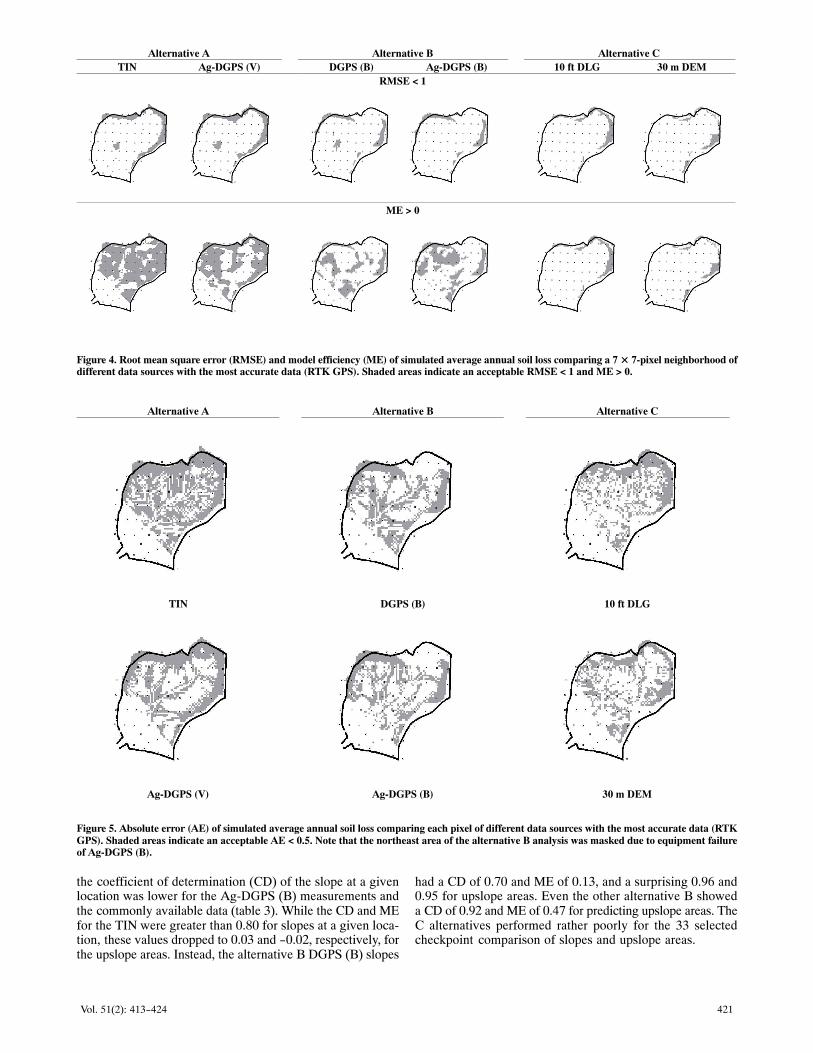
The quantitative filter test for RMSE and ME demon‐strates the relative difference of acceptance areas among al‐ternative data sets in comparison to the most accurate RTKGPS data. The RMSE filter map with an acceptance of anRMSE < 1 (fig. 4) shows that both alternatives in A and theDGPS (B) of alternative B have similar acceptable predic‐tions for upper hillslope areas around the watershed bound‐ary. However, most of the map has RMSE of 1 and higher.The MEFV shows its strength when using an ME > 0 (fig. 4);in this case, the TIN data set shows the largest area of agree‐ment with the RTK GPS data. It is now clear that both alterna‐tives in A are more accurate than alternatives in B. Eventhough the 10 ft DLG was able to identify the hillslope areasof interest, both alternatives in C show almost no agreementwithin the watershed in comparison to the soil loss predic‐

tions based on the RTK GPS unit. This indicates that the morea decision‐maker would demand quantitative estimates forsmaller areas within a watershed, the more likely one needsto invest in more accurate topographic measurement systemssuch as a RTK GPS, a photogrammetric derived TIN, or anAg‐DGPS (V) system.

HILLSLOPE LOCATIONS OF INTEREST (0.01 ha)If a site‐specific decision‐maker requires exact soil loss

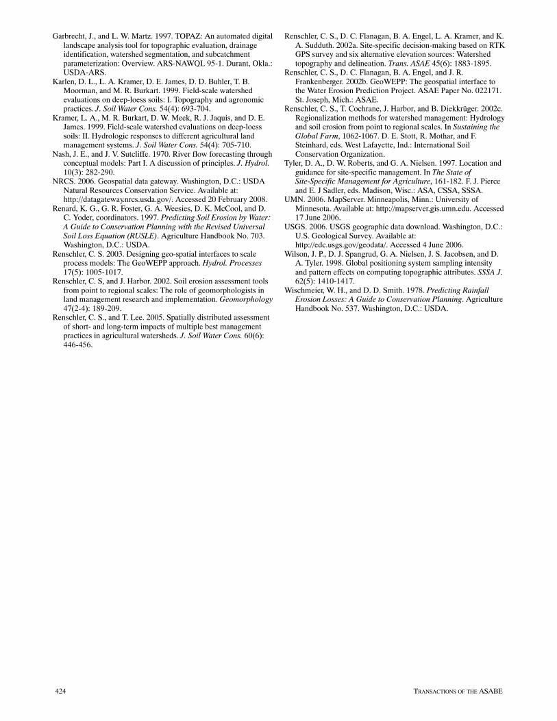
estimates for each raster cell or hillslope location of interest,one has to investigate at the scale of 0.01 ha. An absolute er‐ror analysis of a raster cell‐based analysis indicates that bothalternatives in A have the largest agreement when allowinga maximum absolute error of 50% of the average annual soilloss based on the most accurate RTK GPS unit (fig. 5). TheTIN has the best coverage, while the Ag‐DGPS (V) andDGPS (B) seem to have problems, particularly on the mid‐slope areas. The remaining alternatives indicate only reliablequantitative soil loss estimates below 50% absolute error forthe upper hillslope areas in a raster cell to cell comparison.The main problem here lies in the combination of errors in theslope and upslope (contributing) areas for each raster cell.

A comparison of slopes and upslope areas for all three al‐ternative data sets with the most accurate RTK GPS data forthe 33 selected checkpoints is shown in table 3. While Ren‐schler et al. (2002a) demonstrated that the averages for eleva‐tion of the GPS data sets at a given location were relativelyclose to each other (within about a 1.5 m margin that corre‐sponds to the accuracy levels given by the manufacturers),

421Vol. 51(2): 413-424

Alternative A Alternative B Alternative CTIN Ag‐DGPS (V) DGPS (B) Ag‐DGPS (B) 10 ft DLG 30 m DEM

RMSE < 1

ME > 0

Figure 4. Root mean square error (RMSE) and model efficiency (ME) of simulated average annual soil loss comparing a 7 × 7‐pixel neighborhood ofdifferent data sources with the most accurate data (RTK GPS). Shaded areas indicate an acceptable RMSE < 1 and ME > 0.

Alternative A Alternative B Alternative C

TIN DGPS (B) 10 ft DLG

Ag‐DGPS (V) Ag‐DGPS (B) 30 m DEM

Figure 5. Absolute error (AE) of simulated average annual soil loss comparing each pixel of different data sources with the most accurate data (RTKGPS). Shaded areas indicate an acceptable AE < 0.5. Note that the northeast area of the alternative B analysis was masked due to equipment failureof Ag‐DGPS (B).

the coefficient of determination (CD) of the slope at a givenlocation was lower for the Ag‐DGPS (B) measurements andthe commonly available data (table 3). While the CD and MEfor the TIN were greater than 0.80 for slopes at a given loca‐tion, these values dropped to 0.03 and -0.02, respectively, forthe upslope areas. Instead, the alternative B DGPS (B) slopes

had a CD of 0.70 and ME of 0.13, and a surprising 0.96 and0.95 for upslope areas. Even the other alternative B showeda CD of 0.92 and ME of 0.47 for predicting upslope areas. TheC alternatives performed rather poorly for the 33 selectedcheckpoint comparison of slopes and upslope areas.

422 TRANSACTIONS OF THE ASABE

Table 3. Slopes and upslope areas in flow direction at 33 checkpoints based on different data sets.[a]

Method(applicability) Data Set

Slopes Upslope Contributing AreasCD RMSE ME CD RMSE ME

Alternative ATIN 0.8560 0.1479 0.8007 0.0253 3.0772 ‐0.0221

Ag‐DGPS (V) 0.5101 0.3743 ‐0.2768 0.0033 8.7387 ‐7.2429

Alternative BDGPS (B) 0.7011 0.3081 0.1295 0.9584 0.6719 0.9524

Ag‐DGPS (B) 0.2535 0.4321 ‐0.7123 0.9229 2.2495 0.4666

Alternative C10 ft DLG 0.1325 0.5522 ‐1.6784 0.2393 3.1303 ‐0.047130 m DEM 0.1446 0.4551 ‐0.8188 0.0800 3.4976 ‐0.3072

[a] For averages and standard deviations, see Renschler et al. (2002a); CD = coefficient of determination (r2), RMSE = root mean square error, and ME =model efficiency.

Table 4. Soil loss in flow direction at 33 checkpoints based on different data sets.

Method(applicability) Data Set

Average AnnualSoil Loss

(t ha‐1 year‐1)

StandardDeviation

(%)CD(r2) RMSE ME

Most accurate RTK GPS 10.91 9.67 n.a. n.a. n.a.

Alternative ATIN 10.85 9.40 0.5237 0.6403 0.4624

Ag‐DGPS (V) 5.23 4.62 0.2402 0.9224 ‐0.1156

Alternative BDGPS (B) 5.94 4.93 0.4092 0.8070 0.1275

Ag‐DGPS (B) 9.22 11.31 0.2000 1.0193 ‐0.3921

Alternative C10 ft DLG 14.28 15.49 0.0732 1.4777 ‐1.818730 m DEM 15.30 12.89 0.2609 1.1236 ‐0.8297

Table 5. Overall ranking of average annual runoff, sediment yield, and soil erosion predictions at various scales of interest.[a]

Method(applicability) Data Set

Contributing Areas of Interest,>4 ha

Hillslope Areas of Interest,0.5 ha

Hillslope Locations of Interest,0.01 ha (100 m2)

Area RunoffSediment

Yield Circles Moving filterAll

pixels 33 selected pixelsMost Accurate RTK GPS 1 4 2 1 RMSE ME AE CD RMSE ME

Alternative ATIN 2 5 4 2 2 1 1 1 1 1

Ag‐DGPS (V) 5 7 7 7 1 2 2 4 3 3

Alternative BDGPS (B) 6 6 6 6 3 4 3 2 2 2

Ag‐DGPS (B) 7 3 3 4 4 3 4 5 4 4

Alternative C10 ft DLG 3 1 1 2 5 5 5 6 6 630 m DEM 4 2 5 5 6 6 6 3 5 5

[a] Methods of comparison to the most accurate RTK GPS data set: RMSE = root mean square error, ME = model efficiency, and AE = absolute error.

In terms of soil loss predictions at the 33 checkpoints, theaverages and standard deviations showed large differencesamong alternatives (table 4). While the RTK GPS and theTIN produced the best average values in this regard, the otheralternatives were scattered around these averages in a widerange. The TIN and DGPS (B) showed the best results withthe highest CDs, the lowest RMSEs, and positive ME values.The best alternative was the TIN, which had an ME of 0.46for soil loss. All other alternatives performed comparativelypoorly for the selected 33 checkpoints.

SOIL EROSION PREDICTIONS ACROSS SCALES

A comprehensive ranking of performance of all alterna‐tives across scales indicated that the TIN data offers the bestalternative compared to the survey‐grade RTK GPS measure‐ments at all scales of interest (table 5). Surprisingly, the com‐monly available 10 ft contour lines from USGS are the nextbest alternative if one were only interested in runoff and sedi‐ment yield predictions of smaller subwatersheds larger than4 ha and the identification of critical areas within the 30 hawatershed. The TIN and the Ag‐DGPS (B) offer the best soilloss prediction at smaller scales.

A ranking of all the alternatives providing topographic in‐formation through elevation and their products for the pointscale, such as slopes, upslope areas, and soil loss, reveals avery comprehensive picture about error or uncertainty propa‐gation through the data processing. The TIN and DGPS (B)

data sets show the most consistent ranking among the topthree positions in the comparison with the most accurate RTKGPS data (table 6). Assuming that the variability of weather,soils, and land cover parameters are negligible, and that thesoil loss in this watershed can be considered as a function in‐cluding the slope and upstream contributing areas at a partic‐ular location, it seems that accurate representation of thesecombined two parameters provides the basis for accurate soilloss prediction. Therefore, the TIN and DGPS (B) come in asthe two top alternatives compared to the RTK GPS measure‐ments for elevation and its derivatives in the data processingand modeling sequence.

We are aware that the methodology presented here wastested on only one small watershed with steep slopes, typicalof highly erodible land, but atypical of many of the agricul‐tural lands in the U.S. to which WEPP might be applied. Theresults in much flatter terrain would have been significantlyinfluenced by the DGPS measurement variations due to GPSsatellites in view and the availability of beacon correctionsignals (distance to beacon).

SUMMARY AND CONCLUSIONSThe use of digital topographic data from commonly avail‐

able data sources and precision farming GPS data offers soiland water conservation decision‐makers the possibility of

423Vol. 51(2): 413-424

Table 6. Overall ranking of quantitative values on elevation, slopes, upslope areas, andsoil loss for 33 checkpoints (hillslope locations of interest) based on different data sets.[a]

Method(applicability) Data Set Elevation[b] Slopes Upslope Areas Soil Loss

OverallCumulative Ranks

Most Accurate RTK GPS CD RMSE ME CD RMSE ME CD RMSE ME CD RMSE ME CD RMSE ME

Alternative ATIN 1 4 4 1 1 1 5 3 3 1 1 1 8 9 9

Ag‐DGPS (V) 3 2 2 3 3 3 6 6 6 4 3 3 16 14 12

Alternative BDGPS (B) 2 1 1 2 2 2 1 1 1 2 2 2 7 6 6

Ag‐DGPS (B) 5 3 3 4 4 4 2 2 2 5 4 4 16 15 13

Alternative C10 ft DLG 4 5 5 6 6 6 3 4 4 6 6 6 19 21 2130 m DEM 6 6 6 5 5 5 4 5 5 3 5 5 18 21 16

[a] CD = coefficient of determination (r2), RMSE = root mean square error, and ME = model efficiency.[b] See quantitative values in Renschler et al. (2002a).

using this topographic data for running soil erosion predic‐tion tools such as the Water Erosion Prediction Project(WEPP) model. The analysis of accurate topographical rep‐resentation in the raw elevation data, the discretization of to‐pographical parameters, the distributed simulation output,and the simulation results for the watershed outlet are criticalto site‐specific decision‐making. In addition to the choice ofthe target raster size and the most appropriate interpolationalgorithm, the variability of elevation representation, topo‐graphical parameter discretization, their impact on modelpredictions, and comparison with observed values based ona wide range of available data sources need to be investigatedin each watershed analysis using GIS.

This study demonstrates that not only the accuracy of thedata source but also the appropriate handling and consequentanalysis of topographical data within the GIS model environ‐ment have an impact on useful prediction results. This studyillustrates that survey‐grade RTK GPS data, a photogram‐metric survey (TIN), to some extent precision farming‐typedifferential GPS, and even interpolated DEMs based on com‐monly available 10 ft contour lines from USGS topographicmaps can be used for effective soil loss estimates in small wa‐tersheds. The results show that the more precise topographicmeasurements with an RTK GPS, a photogrammetric survey(TIN), and DGPS yield more precise on‐site soil loss predic‐tions at all scales ranging from individual raster cells (0.01ha) and hillslope areas (0.5 ha) to small watersheds (>4 ha).The results at the small watershed scale demonstrate thatDEMs based on USGS 10 ft contour lines from commonlyavailable data can be as good as the most accurate data sets(RTK GPS or TIN) in predicting average annual off‐site run‐off (-18.3% error) and sediment yield (-2.7% error) with theWEPP model for the upslope contributing areas of 4 ha orlarger within the 30 ha watershed. As with the RTK GPS andTIN data sets, the contours also allowed successful identifi‐cation of all 11 hillslope areas of concern with known soil loss(10) or deposition (1) problems. In addition to this visual in‐spection of hillslope areas of interest, at the individual rastercell scale, two newly developed statistical filters utilizing theroot mean square error (RMSE) and Nash‐Sutcliffe model ef‐ficiency (ME) values allowed visualization and quantifica‐tion of the spatially distributed accuracy in predicting theobserved values within the watershed (TIN had largest areawith ME > 0 when compared with RTK GPS). An overallranking based on quantitative values for predicted elevations,slopes, upslope areas, and simulated soil loss values for33�checkpoints revealed that the best alternative sources oftopographic data to substitute for survey‐grade RTK GPSwere the photogrammetric survey (TIN) or the DGPS with abeacon correction.

ACKNOWLEDGEMENTSWe want to thank Bernard A. Engel of the Department of

Agricultural and Biological Engineering, Purdue University,West Lafayette, Indiana, for the discussion of the results. Wealso want to acknowledge Kenneth A. Sudduth, Robert L.Mahurin, and Michael J. Krumpelman of the USDA‐ARSCropping Systems and Water Quality Research Unit, Colum‐bia, Missouri, for their efforts in gathering the RTK GPS fielddata. The authors especially want to thank Larry A. Kramer,who just recently retired from the USDA‐ARS Deep LoessResearch Station at Treynor, Iowa, for his service and con‐tributions to establish extremely valuable long‐time soil ero‐sion measurement series for the experimental watersheds.The College of Arts and Sciences, University at Buffalo, andthe USDA ARS National Soil Erosion Research Laboratoryprovided financial assistance to publish this research.

REFERENCESBoB. 1947. United States National Map Accuracy Standards.

Revised 17 June 1947. Washington, D.C.: U.S. Bureau of theBudget.

Clark, R. L., and R. Lee. 1998. Development of topographical mapsfor precision farming with kinematic GPS. Trans. ASAE 41(4):909‐916.

Cochrane, T. A., and D. C. Flanagan. 1999. Assessing water erosionin small watersheds using WEPP with GIS and digital elevationmodels. J. Soil Water Cons. 54(4): 678‐685.

Cochrane, T. A., and D. C. Flanagan. 2003. Representative hillslopemethods for applying the WEPP model with DEMs and GIS.Trans. ASAE 46(4): 1041‐1049.

ESRI. 2006. ArcInfo 8 - User's Guide. Ver. 8. Redlands, Cal.:Environmental Systems Research Institute, Inc. Available at:www.esri.com/software/arcgis/arcinfo/. Accessed 17 June 2006.

Flanagan, D. C., and M. A. Nearing, eds. 1995. USDA‐WaterErosion Prediction Project: Hillslope profile and watershedmodel documentation. NSERL Report No. 10. West Lafayette,Ind.: USDA‐ARS National Soil Erosion Research Laboratory.

Flanagan, D. C., J. C. Ascough II, M. A. Nearing, and J. M. Laflen.2001. Chapter 7: The Water Erosion Prediction Project (WEPP)Model. In Landscape Erosion and Evolution Modeling,145‐199. R. S. Harmon and W. W. Doe III, eds. New York, N.Y.:Kluwer Academic / Plenum Publishers.

Flanagan, D. C., J. R. Frankenberger, C. S. Renschler, and B. A.Engel. 2004a. Development of web‐based GIS interfaces forapplication of the WEPP model. In Proc. ISCO 2004: 13th Intl.Soil Conserv. Org. Conf., Paper No. 419. Brisbane, Queensland,Australia: International Soil Conservation Organization.

Flanagan, D. C., J. R. Frankenberger, and B. A. Engel. 2004b.Web‐based GIS application of the WEPP model. ASAE PaperNo. 042024. St. Joseph, Mich.: ASAE.

424 TRANSACTIONS OF THE ASABE

Garbrecht, J., and L. W. Martz. 1997. TOPAZ: An automated digitallandscape analysis tool for topographic evaluation, drainageidentification, watershed segmentation, and subcatchmentparameterization: Overview. ARS‐NAWQL 95‐1. Durant, Okla.:USDA‐ARS.

Karlen, D. L., L. A. Kramer, D. E. James, D. D. Buhler, T. B.Moorman, and M. R. Burkart. 1999. Field‐scale watershedevaluations on deep‐loess soils: I. Topography and agronomicpractices. J. Soil Water Cons. 54(4): 693‐704.

Kramer, L. A., M. R. Burkart, D. W. Meek, R. J. Jaquis, and D. E.James. 1999. Field‐scale watershed evaluations on deep‐loesssoils: II. Hydrologic responses to different agricultural landmanagement systems. J. Soil Water Cons. 54(4): 705‐710.

Nash, J. E., and J. V. Sutcliffe. 1970. River flow forecasting throughconceptual models: Part I. A discussion of principles. J. Hydrol.10(3): 282‐290.

NRCS. 2006. Geospatial data gateway. Washington, D.C.: USDANatural Resources Conservation Service. Available at:http://datagateway.nrcs.usda.gov/. Accessed 20 February 2008.

Renard, K. G., G. R. Foster, G. A. Weesies, D. K. McCool, and D.C. Yoder, coordinators. 1997. Predicting Soil Erosion by Water:A Guide to Conservation Planning with the Revised UniversalSoil Loss Equation (RUSLE). Agriculture Handbook No. 703.Washington, D.C.: USDA.

Renschler, C. S. 2003. Designing geo‐spatial interfaces to scaleprocess models: The GeoWEPP approach. Hydrol. Processes17(5): 1005‐1017.

Renschler, C. S, and J. Harbor. 2002. Soil erosion assessment toolsfrom point to regional scales: The role of geomorphologists inland management research and implementation. Geomorphology47(2‐4): 189‐209.

Renschler, C. S., and T. Lee. 2005. Spatially distributed assessmentof short‐ and long‐term impacts of multiple best managementpractices in agricultural watersheds. J. Soil Water Cons. 60(6):446‐456.

Renschler, C. S., D. C. Flanagan, B. A. Engel, L. A. Kramer, and K.A. Sudduth. 2002a. Site‐specific decision‐making based on RTKGPS survey and six alternative elevation sources: Watershedtopography and delineation. Trans. ASAE 45(6): 1883‐1895.

Renschler, C. S., D. C. Flanagan, B. A. Engel, and J. R.Frankenberger. 2002b. GeoWEPP: The geospatial interface tothe Water Erosion Prediction Project. ASAE Paper No. 022171.St. Joseph, Mich.: ASAE.

Renschler, C. S., T. Cochrane, J. Harbor, and B. Diekkrüger. 2002c.Regionalization methods for watershed management: Hydrologyand soil erosion from point to regional scales. In Sustaining theGlobal Farm, 1062‐1067. D. E. Stott, R. Mothar, and F.Steinhard, eds. West Lafayette, Ind.: International SoilConservation Organization.

Tyler, D. A., D. W. Roberts, and G. A. Nielsen. 1997. Location andguidance for site‐specific management. In The State ofSite‐Specific Management for Agriculture, 161‐182. F. J. Pierceand E. J Sadler, eds. Madison, Wisc.: ASA, CSSA, SSSA.

UMN. 2006. MapServer. Minneapolis, Minn.: University ofMinnesota. Available at: http://mapserver.gis.umn.edu. Accessed17 June 2006.

USGS. 2006. USGS geographic data download. Washington, D.C.:U.S. Geological Survey. Available at:http://edc.usgs.gov/geodata/. Accessed 4 June 2006.

Wilson, J. P., D. J. Spangrud, G. A. Nielsen, J. S. Jacobsen, and D.A. Tyler. 1998. Global positioning system sampling intensityand pattern effects on computing topographic attributes. SSSA J.62(5): 1410‐1417.

Wischmeier, W. H., and D. D. Smith. 1978. Predicting RainfallErosion Losses: A Guide to Conservation Planning. AgricultureHandbook No. 537. Washington, D.C.: USDA.