Jeff Valenti

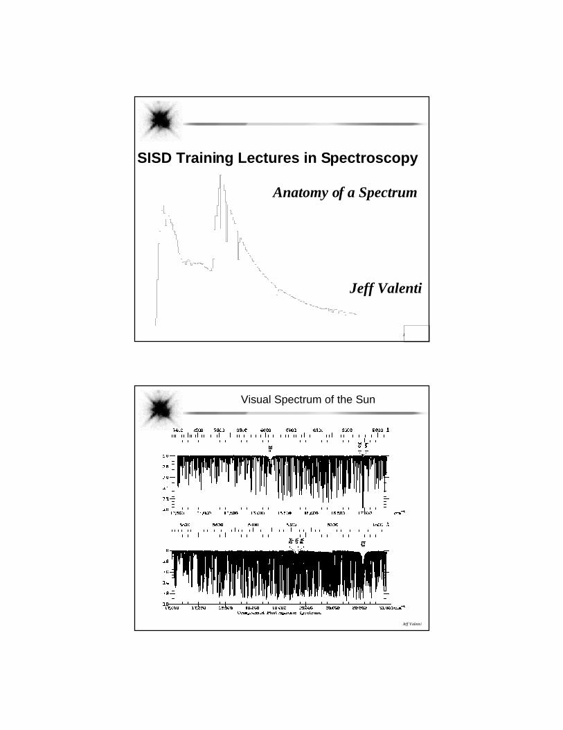
SISD Training Lectures in Spectroscopy

Jeff Valenti

Anatomy of a Spectrum

Jeff Valenti

Visual Spectrum of the Sun

Jeff Valenti

Blue Spectrum of the Sun

Jeff Valenti

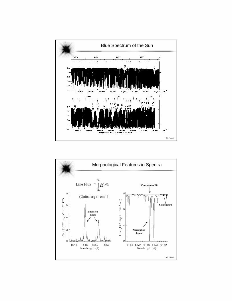
Morphological Features in Spectra

EmissionLines

AbsorptionLines

Continuum Fit

Continuum

Line Flux = ∫ λ λλ

λF d

1

2

)cm s erg :(Units -2-1

Jeff Valenti

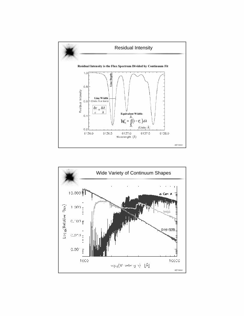
Residual Intensity

Residual Intensity is the Flux Spectrum Divided by Continuum Fit

Line Width

Lin

e D

epth

km/s) or A :(Unitso

λλ∆=∆

c

v

eqW r d= −( )∫ 1

1

2

λ

λ

λλ

Equivalent Width:

)A :(Unitso

Jeff Valenti

Wide Variety of Continuum Shapes

Jeff Valenti

Planck Function

« Assumptions¥ Uniform temperature source¥ Source is opaque

« Mathematical description

( ) 1/exp/2 52

−=

kThchc

Bλ

λλ

Units : erg

s cm A ster 2 o

Emitting Area

h Planck Constant 6.63 erg s= = × −10 27

c Speed of Light 3.00 cm s-1= = ×1010

k Boltzmann Constant 1.38 erg K-1= = × −10 16

( )cmLight ofh Wavelengt =λ( )K eTemperatur Uniform =T

Jeff Valenti

Computed Blackbody Spectra

WienLaw

( ) 1/exp/2 52

−=

kThc

hcB

λλ

λ

Rayleigh-JeansTail

Jeff Valenti

Wien Displacement Law

« Blackbody peak wavelength inversely proportional to temperature« Find peak wavelength by solving:

( ) 1/exp/2 52

−=

kThchc

Bλ

λλ

0d

d=

λλB

where

( ) ye y =− −15 where kT

hcy

pkλ=

97.4 :solution Numerical =y

λ pk cm KT = 0 29.

Wien Law: T = → =300 10 K mpkλ µT = → =3000 1 K mpkλ µT = → =30 000 0 1, . K mpkλ µ

Jeff Valenti

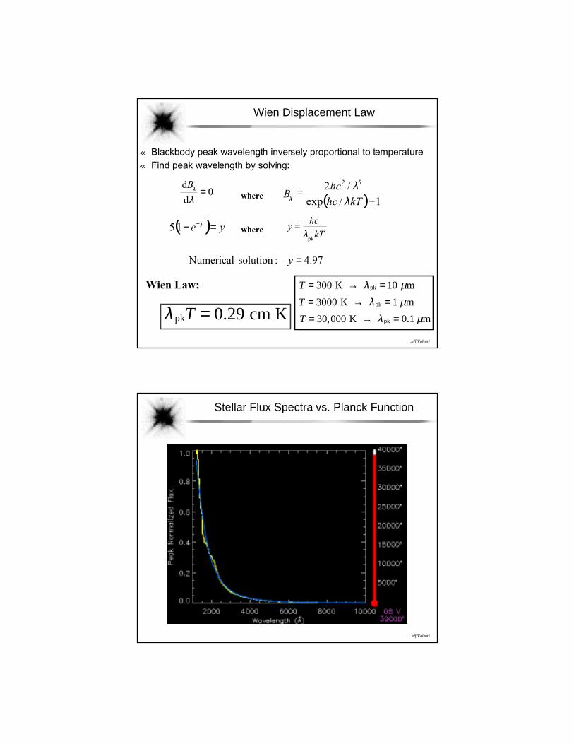
Stellar Flux Spectra vs. Planck Function

Jeff Valenti

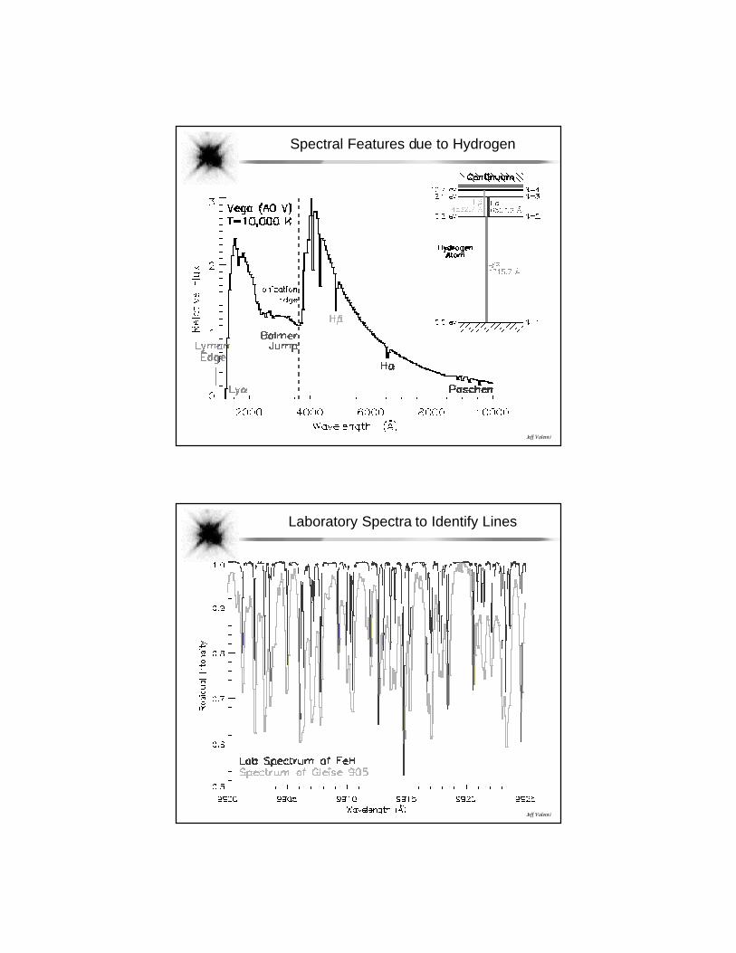
Spectral Features due to Hydrogen

Jeff Valenti

Laboratory Spectra to Identify Lines

Jeff Valenti

Line Identification References

« Labelled Spectral Atlases¥ Solar Photosphere, 0.36-22 micron (Wallace et al. 1991-1999)¥ Sunspot, 0.39-21 micron (Wallace et al. 1992-2000)¥ Arcturus (K1 III), 0.37-5.3 micron (Hinkle et al. 1995-2000)

« Printed Line Lists¥ Atomic and Ionic Spectrum Lines Below 2000 A (Kelly 1987)¥ FUV lines in solar spectrum (Sandlin et al. 1986, ApJS, 61, 801)¥ Ultraviolet Multiplet Table (Moore 1950)¥ A Multiplet Table of Astrophysical Interest (Moore 1945)

« Electronic Media¥ Kurucz CD-ROM Series (1993-1999)¥ Vienna Atomic Line Database (VALD, Kupka et al. 1999, A&AS, 138)

http://www.astro.univie.ac.at./~vald/

¥ Atomic Data for Resonance Absorption Lines (Morton 1991, ApJS)http://www.hia.nrc.ca/staff/dcm/atomic_data.html

Jeff Valenti

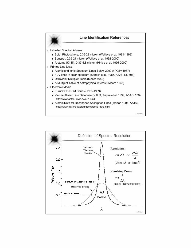
Definition of Spectral Resolution

IntrinsicThoriumProfile

Observed Profile

FWHM

λ∆

λ

Resolution:

Rc= ∆ ∆λ λλ

or

)s kmor A :(Units 1-o

Resolving Power:

λλ

∆=R

ess)Dimensionl :(Units

Jeff Valenti

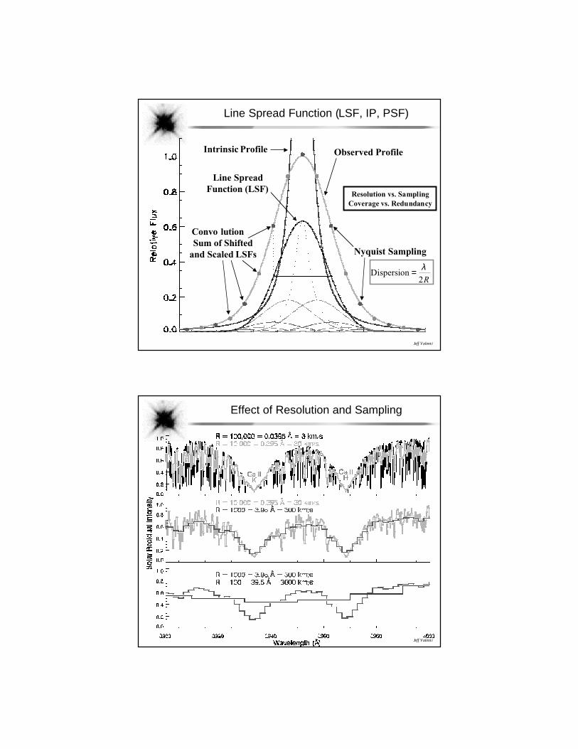
Line Spread Function (LSF, IP, PSF)

Intrinsic Profile

Line SpreadFunction (LSF)

Sum of Shiftedand Scaled LSFs

Observed Profile

Nyquist Sampling

R2 Dispersion

λ=

Convo lution

Resolution vs. SamplingCoverage vs. Redundancy

Jeff Valenti

Effect of Resolution and Sampling

Jeff Valenti

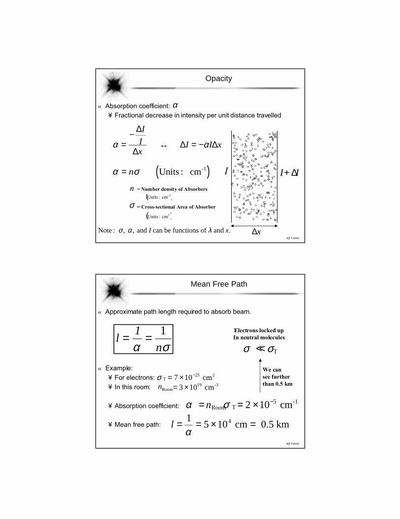
Opacity

« Absorption coefficient:¥ Fractional decrease in intensity per unit distance travelled

α

α α=−

↔ = −

∆

∆∆ ∆

I

Ix

I I x

∆x

I I I+ ∆α σ= ( )n Units : cm-1

n = Number density of Absorbers

σ = Cross-sectional Area of Absorber

( )-3cm :Units

( )2cm :Units

Note : , , and can be functions of and .σ α λI x

Jeff Valenti

Mean Free Path

« Approximate path length required to absorb beam.

« Example:¥ For electrons:¥ In this room:

¥ Absorption coefficient:

¥ Mean free path:

l1

n= =

α σ1

σ T2 cm= × −7 10 25

nRoom-3 cm= ×3 1019

α σ= = × −nRoom T-1 cm2 10 5

l = = × =15 104

α cm 0.5 km

Electrons locked upIn neutral molecules

σ σ<< T

We cansee furtherthan 0.5 km

Jeff Valenti

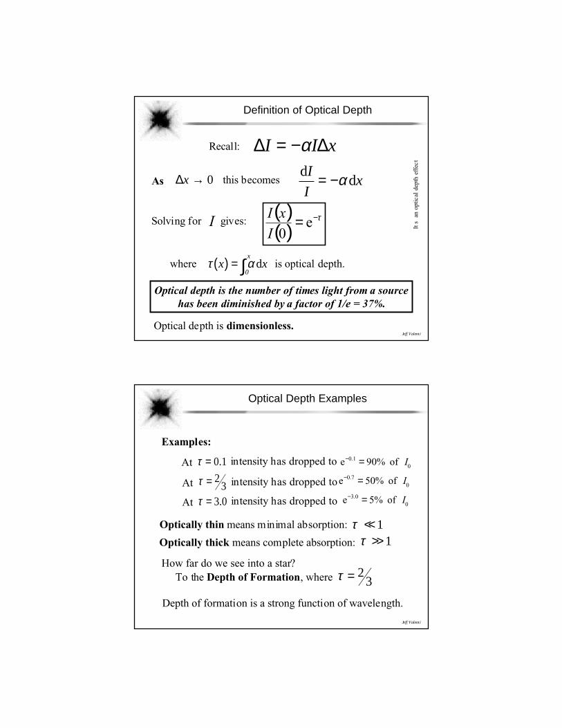
Definition of Optical Depth

Recall: ∆ ∆I I x= −α

As ∆x → 0 this becomesd

dI

Ix= −α

Solving for I gives:( )( )

τ−= e0I

xI

where τ αx x0

x

( ) = ∫ d is optical depth.

Optical depth is the number of times light from a sourcehas been diminished by a factor of 1/e = 37%.

Optical depth is dimensionless.

Its

an o

ptic

al d

epth

eff

ect

Jeff Valenti

Optical Depth Examples

At τ = 0 1. intensity has dropped to0

1.0 of %90e I=−

At τ = 23 intensity has dropped to 0

7.0 of %50e I=−

At τ = 3 0. intensity has dropped to 00.3 of %5e I=−

Examples:

Optically thin means minimal absorption: τ <<1Optically thick means complete absorption: τ >>1

How far do we see into a star?To the Depth of Formation, where τ = 2

3

Depth of formation is a strong function of wavelength.

Jeff Valenti

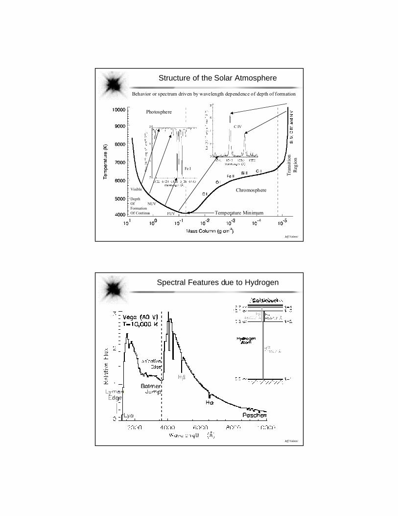
Structure of the Solar Atmosphere

Chromosphere

Photosphere

Tra

nsit

ion

Reg

ion

Temperature Minimum

Visible

NUV

FUV

DepthOfFormationOf Continua

C IV

Fe I

Behavior or spectrum driven by wavelength dependence of depth of formation

Jeff Valenti

Spectral Features due to Hydrogen

Jeff Valenti

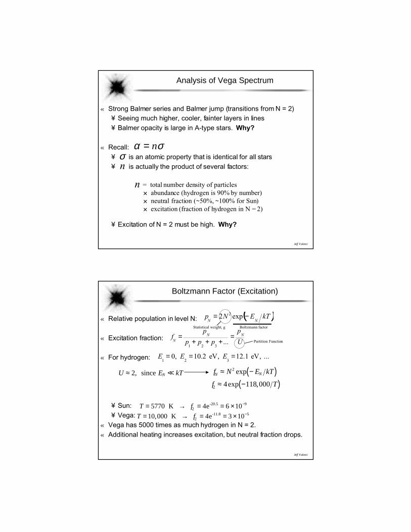
Analysis of Vega Spectrum

« Strong Balmer series and Balmer jump (transitions from N = 2)¥ Seeing much higher, cooler, fainter layers in lines¥ Balmer opacity is large in A-type stars. Why?

« Recall:¥ is an atomic property that is identical for all stars¥ is actually the product of several factors:

¥ Excitation of N = 2 must be high. Why?

α σ= nσn

n = total number density of particles× abundance (hydrogen is 90% by number)× neutral fraction (~50%, ~100% for Sun)× excitation (fraction of hydrogen in N = 2)

Jeff Valenti

Boltzmann Factor (Excitation)

« Relative population in level N:

« Excitation fraction:

« For hydrogen:

¥ Sun:¥ Vega:

« Vega has 5000 times as much hydrogen in N = 2.« Additional heating increases excitation, but neutral fraction drops.

( )kTENpNN

−= exp2 2

Statistical weight, g Boltzmann factor

U

p

ppp

pf NNN

=+++

=...

321Partition Function

... ,Ve 1.12 ,Ve 2.10 ,0321

=== EEE

U E kTN≈ <<2, since f N E kTN N≈ −( )2 exp

f T2 4 118 000≈ −( )exp ,

T f= → = = × −5770 4 6 1029 K e-20.5

T f= → = = × −10 000 4 3 1025, K e-11.8

Jeff Valenti

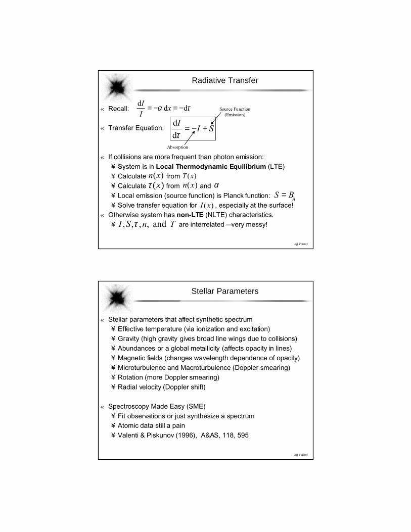
Radiative Transfer

« Recall:

« Transfer Equation:

« If collisions are more frequent than photon emission:¥ System is in Local Thermodynamic Equilibrium (LTE)¥ Calculate from¥ Calculate from and¥ Local emission (source function) is Planck function:¥ Solve transfer equation for , especially at the surface!

« Otherwise system has non-LTE (NLTE) characteristics.¥ are interrelated — very messy!

τα d dd −=−= xII

SII +−=τd

d

Absorption

Source Function(Emission)

)(xnτ ( )x

)(xT)(xn α

λBS =)(xI

TnSI and ,,,, τ

Jeff Valenti

Stellar Parameters

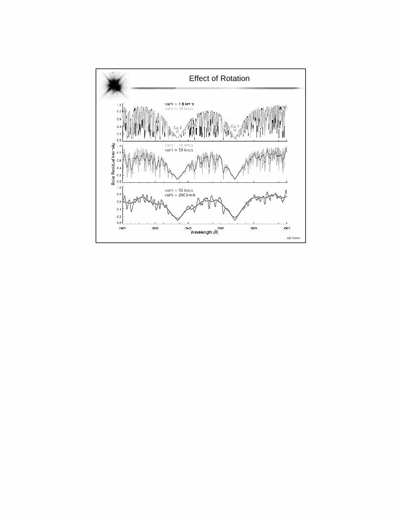
« Stellar parameters that affect synthetic spectrum¥ Effective temperature (via ionization and excitation)¥ Gravity (high gravity gives broad line wings due to collisions)¥ Abundances or a global metallicity (affects opacity in lines)¥ Magnetic fields (changes wavelength dependence of opacity)¥ Microturbulence and Macroturbulence (Doppler smearing)¥ Rotation (more Doppler smearing)¥ Radial velocity (Doppler shift)

« Spectroscopy Made Easy (SME)¥ Fit observations or just synthesize a spectrum¥ Atomic data still a pain¥ Valenti & Piskunov (1996), A&AS, 118, 595

Jeff Valenti

Effect of Rotation