Sirindhorn International Institute of Technology ECS 315 ... 2013 ALL.pdf · ... Probability and...
230
Sirindhorn International Institute of Technology Thammasat University School of Information, Computer and Communication Technology ECS 315: Probability and Random Processes Asst. Prof. Dr. Prapun Suksompong [email protected] October 3, 2013 This note covers fundamental concepts in probability and a brief touch on random processes for undergraduate students in electronics and communication engineering. It is designed for a one-semester course at Sirindhorn International Institute of Technology (SIIT). Despite my best endeavors, this note will not be error-free. I hope that none of the mistakes are misleading. But since probability can be a subtle subject, if I have made some slips of principle, do not hesitate to tell me about them. Greater minds than mine have erred in this field. 1
-
Upload
nguyenxuyen -
Category
Documents
-
view
219 -
download
0
Transcript of Sirindhorn International Institute of Technology ECS 315 ... 2013 ALL.pdf · ... Probability and...

Sirindhorn International Institute of Technology
Thammasat University
School of Information, Computer and Communication Technology
ECS 315: Probability and Random Processes
Asst. Prof. Dr. Prapun [email protected]
October 3, 2013
This note covers fundamental concepts in probability and a brief touch onrandom processes for undergraduate students in electronics and communicationengineering. It is designed for a one-semester course at Sirindhorn InternationalInstitute of Technology (SIIT).
Despite my best endeavors, this note will not be error-free. I hope that noneof the mistakes are misleading. But since probability can be a subtle subject,if I have made some slips of principle, do not hesitate to tell me about them.Greater minds than mine have erred in this field.
1

Contents
1 Probability and You 41.1 Randomness . . . . . . . . . . . . . . . . . . . . . . . . . . . . . 41.2 Background on Some Frequently Used Examples . . . . . . . . . 61.3 A Glimpse at Probability Theory . . . . . . . . . . . . . . . . . 8
2 Review of Set Theory 12
3 Classical Probability 17
4 Enumeration / Combinatorics / Counting 204.1 Four Principles . . . . . . . . . . . . . . . . . . . . . . . . . . . 204.2 Four Kinds of Counting Problems . . . . . . . . . . . . . . . . . 264.3 Binomial Theorem and Multinomial Theorem . . . . . . . . . . 364.4 Famous Example: Galileo and the Duke of Tuscany . . . . . . . 384.5 Application: Success Runs . . . . . . . . . . . . . . . . . . . . . 39
5 Probability Foundations 44
6 Event-based Independence and Conditional Probability 536.1 Event-based Conditional Probability . . . . . . . . . . . . . . . 536.2 Event-based Independence . . . . . . . . . . . . . . . . . . . . . 666.3 Bernoulli Trials . . . . . . . . . . . . . . . . . . . . . . . . . . . 72
7 Random variables 78
8 Discrete Random Variables 838.1 PMF: Probability Mass Function . . . . . . . . . . . . . . . . . 848.2 CDF: Cumulative Distribution Function . . . . . . . . . . . . . 878.3 Families of Discrete Random Variables . . . . . . . . . . . . . . 908.4 Some Remarks . . . . . . . . . . . . . . . . . . . . . . . . . . . 100
9 Expectation and Variance 1019.1 Expectation of Discrete Random Variable . . . . . . . . . . . . . 1019.2 Function of a Discrete Random Variable . . . . . . . . . . . . . 1069.3 Expectation of a Function of a Discrete Random Variable . . . . 1079.4 Variance and Standard Deviation . . . . . . . . . . . . . . . . . 110
10 Continuous Random Variables 11510.1 From Discrete to Continuous Random Variables . . . . . . . . . 11510.2 Properties of PDF and CDF for Continuous Random Variables . 11910.3 Expectation and Variance . . . . . . . . . . . . . . . . . . . . . 12410.4 Families of Continuous Random Variables . . . . . . . . . . . . 127
10.4.1 Uniform Distribution . . . . . . . . . . . . . . . . . . . . 12710.4.2 Gaussian Distribution . . . . . . . . . . . . . . . . . . . 129
2
10.4.3 Exponential Distribution . . . . . . . . . . . . . . . . . . 13610.5 Function of Continuous Random Variables: SISO . . . . . . . . 139
11 Multiple Random Variables 14411.1 A Pair of Discrete Random Variables . . . . . . . . . . . . . . . 14411.2 Extending the Definitions to Multiple RVs . . . . . . . . . . . . 15711.3 Function of Discrete Random Variables . . . . . . . . . . . . . . 15911.4 Expectation of Function of Discrete Random Variables . . . . . 16111.5 Linear Dependence . . . . . . . . . . . . . . . . . . . . . . . . . 16411.6 Pairs of Continuous Random Variables . . . . . . . . . . . . . . 17111.7 Function of a Pair of Continuous Random Variables: MISO . . . 177
12 Three Types of Random Variables 184
13 Transform methods: Characteristic Functions 188
14 Limiting Theorems 19114.1 Law of Large Numbers (LLN) . . . . . . . . . . . . . . . . . . . 19114.2 Central Limit Theorem (CLT) . . . . . . . . . . . . . . . . . . . 193
15 Random Vector 198
16 Introduction to Stochastic Processes (Random Processes) 20116.1 Autocorrelation Function and WSS . . . . . . . . . . . . . . . . 20416.2 Power Spectral Density (PSD) . . . . . . . . . . . . . . . . . . . 207
A Math Review 212A.1 Summations . . . . . . . . . . . . . . . . . . . . . . . . . . . . . 212A.2 Inequalities . . . . . . . . . . . . . . . . . . . . . . . . . . . . . 215A.3 Calculus . . . . . . . . . . . . . . . . . . . . . . . . . . . . . . . 220
3
Sirindhorn International Institute of Technology
Thammasat University
School of Information, Computer and Communication Technology
ECS315 2013/1 Part I.1 Dr.Prapun
1 Probability and You
Whether you like it or not, probabilities rule your life. If you haveever tried to make a living as a gambler, you are painfully awareof this, but even those of us with more mundane life stories areconstantly affected by these little numbers.
Example 1.1. Some examples from daily life where probabilitycalculations are involved are the determination of insurance premi-ums, the introduction of new medications on the market, opinionpolls, weather forecasts, and DNA evidence in courts. Probabil-ities also rule who you are. Did daddy pass you the X or the Ychromosome? Did you inherit grandma’s big nose?
Meanwhile, in everyday life, many of us use probabilities in ourlanguage and say things like “I’m 99% certain” or “There is a one-in-a-million chance” or, when something unusual happens, ask therhetorical question “What are the odds?”. [17, p 1]
1.1 Randomness
1.2. Many clever people have thought about and debated whatrandomness really is, and we could get into a long philosophicaldiscussion that could fill up a whole book. Let’s not. The Frenchmathematician Laplace (1749–1827) put it nicely:
“Probability is composed partly of our ignorance, partlyof our knowledge.”
4
Inspired by Laplace, let us agree that you can use probabilitieswhenever you are faced with uncertainty. [17, p 2]
1.3. Random phenomena arise because of [13]:
(a) our partial ignorance of the generating mechanism
(b) the laws governing the phenomena may be fundamentally ran-dom (as in quantum mechanics; see also Ex. 1.7.)
(c) our unwillingness to carry out exact analysis because it is notworth the trouble
Example 1.4. Communication Systems [23]: The essence ofcommunication is randomness.
(a) Random Source: The transmitter is connected to a randomsource, the output of which the receiver cannot predict withcertainty.
• If a listener knew in advance exactly what a speakerwould say, and with what intonation he would say it,there would be no need to listen!
(b) Noise: There is no communication problem unless the trans-mitted signal is disturbed during propagation or reception ina random way.
(c) Probability theory is used to evaluate the performance of com-munication systems.
Example 1.5. Random numbers are used directly in the transmis-sion and security of data over the airwaves or along the Internet.
(a) A radio transmitter and receiver could switch transmissionfrequencies from moment to moment, seemingly at random,but nevertheless in synchrony with each other.
(b) The Internet data could be credit-card information for a con-sumer purchase, or a stock or banking transaction secured bythe clever application of random numbers.
5

Example 1.6. Randomness is an essential ingredient in games ofall sorts, computer or otherwise, to make for unexpected actionand keen interest.
Example 1.7. On a more profound level, quantum physiciststeach us that everything is governed by the laws of probability.They toss around terms like the Schrodinger wave equation andHeisenberg’s uncertainty principle, which are much too difficult formost of us to understand, but one thing they do mean is that thefundamental laws of physics can only be stated in terms of proba-bilities. And the fact that Newton’s deterministic laws of physicsare still useful can also be attributed to results from the theory ofprobabilities. [17, p 2]
1.8. Most people have preconceived notions of randomness thatoften differ substantially from true randomness. Truly randomdata sets often have unexpected properties that go against intuitivethinking. These properties can be used to test whether data setshave been tampered with when suspicion arises. [21, p 191]
• [14, p 174]: “people have a very poor conception of random-ness; they do not recognize it when they see it and they cannotproduce it when they try”
Example 1.9. Apple ran into an issue with the random shufflingmethod it initially employed in its iPod music players: true ran-domness sometimes produces repetition, but when users heard thesame song or songs by the same artist played back-to-back, theybelieved the shuffling wasn’t random. And so the company madethe feature “less random to make it feel more random,” said Applefounder Steve Jobs. [14, p 175]
1.2 Background on Some Frequently Used Examples
Probabilists love to play with coins and dice. We like the idea oftossing coins, rolling dice, and drawing cards as experiments thathave equally likely outcomes.
1.10. Coin flipping or coin tossing is the practice of throwinga coin in the air to observe the outcome.
6

When a coin is tossed, it does not necessarily fall heads ortails; it can roll away or stand on its edge. Nevertheless, we shallagree to regard “head” (H) and “tail” (T) as the only possibleoutcomes of the experiment. [4, p 7]
• Typical experiment includes
“Flip a coin N times. Observe the sequence of heads andtails” or “Observe the number of heads.”
1.11. Historically, dice is the plural of die , but in modern stan-dard English dice is used as both the singular and the plural. [Ex-cerpted from Compact Oxford English Dictionary.]
• Usually assume six-sided dice
• Usually observe the number of dots on the side facing up-wards.
1.12. A complete set of cards is called a pack or deck.
(a) The subset of cards held at one time by a player during agame is commonly called a hand.
(b) For most games, the cards are assembled into a deck, andtheir order is randomized by shuffling.
(c) A standard deck of 52 cards in use today includes thirteenranks of each of the four French suits.
• The four suits are called spades (♠), clubs (♣), hearts(♥), and diamonds (♦). The last two are red, the firsttwo black.
(d) There are thirteen face values (2, 3, . . . , 10, jack, queen, king,ace) in each suit.
• Cards of the same face value are called of the same kind.
• “court” or face card: a king, queen, or jack of any suit.
7

1.3 A Glimpse at Probability Theory
1.13. Probabilities are used in situations that involve random-ness. A probability is a number used to describe how likelysomething is to occur, and probability (without indefinite arti-cle) is the study of probabilities. It is “the art of being certainof how uncertain you are .” [17, p 2–4] If an event is certainto happen, it is given a probability of 1. If it is certain not tohappen, it has a probability of 0. [7, p 66]
1.14. Probabilities can be expressed as fractions, as decimal num-bers, or as percentages. If you toss a coin, the probability to getheads is 1/2, which is the same as 0.5, which is the same as 50%.There are no explicit rules for when to use which notation.
• In daily language, proper fractions are often used and oftenexpressed, for example, as “one in ten” instead of 1/10 (“onetenth”). This is also natural when you deal with equally likelyoutcomes.
• Decimal numbers are more common in technical and sci-entific reporting when probabilities are calculated from data.Percentages are also common in daily language and often with“chance” replacing “probability.”
• Meteorologists, for example, typically say things like “thereis a 20% chance of rain.” The phrase “the probability of rainis 0.2” means the same thing.
• When we deal with probabilities from a theoretical viewpoint,we always think of them as numbers between 0 and 1, not aspercentages.
• See also 3.5.
[17, p 10]
Definition 1.15. Important terms [13]:
(a) An activity or procedure or observation is called a randomexperiment if its outcome cannot be predicted precisely be-cause the conditions under which it is performed cannot bepredetermined with sufficient accuracy and completeness.
8
• The term “experiment” is to be construed loosely. We donot intend a laboratory situation with beakers and testtubes.
• Tossing/flipping a coin, rolling a dice, and drawing a cardfrom a deck are some examples of random experiments.
(b) A random experiment may have several separately identifiableoutcomes. We define the sample space Ω as a collectionof all possible (separately identifiable) outcomes/results/mea-surements of a random experiment. Each outcome (ω) is anelement, or sample point, of this space.
• Rolling a dice has six possible identifiable outcomes(1, 2, 3, 4, 5, and 6).
(c) Events are sets (or classes) of outcomes meeting some spec-ifications.
• Any1 event is a subset of Ω.
• Intuitively, an event is a statement about the outcome(s)of an experiment.
The goal of probability theory is to compute the probability of var-ious events of interest. Hence, we are talking about a set functionwhich is defined on subsets of Ω.
Example 1.16. The statement “when a coin is tossed, the prob-ability to get heads is l/2 (50%)” is a precise statement.
(a) It tells you that you are as likely to get heads as you are toget tails.
(b) Another way to think about probabilities is in terms of aver-age long-term behavior. In this case, if you toss the coinrepeatedly, in the long run you will get roughly 50% headsand 50% tails.
1For our class, it may be less confusing to allow event A to be any collection of outcomes(, i.e. any subset of Ω).
In more advanced courses, when we deal with uncountable Ω, we limit our interest to onlysome subsets of Ω. Technically, the collection of these subsets must form a σ-algebra.
9

Although the outcome of a random experiment is unpredictable,there is a statistical regularity about the outcomes. What youcannot be certain of is how the next toss will come up. [17, p 4]
1.17. Long-run frequency interpretation : If the probabilityof an event A in some actual physical experiment is p, then webelieve that if the experiment is repeated independently over andover again, then a theorem called the law of large numbers(LLN) states that, in the long run, the event A will happen ap-proximately 100p% of the time. In other words, if we repeat anexperiment a large number of times then the fraction of times theevent A occurs will be close to P (A).
Example 1.18. Return to the coin tossing experiment in Ex. 1.16:
Definition 1.19. Let A be one of the events of a random exper-iment. If we conduct a sequence of n independent trials of thisexperiment, and if the event A occurs in N(A, n) out of these ntrials, then the fraction
is called the relative frequency of the event A in these n trials.
1.20. The long-run frequency interpretation mentioned in 1.17can be restated as
P (A) “=” limn→∞
N(A, n)
n.
1.21. Another interpretation: The probability of an outcome canbe interpreted as our subjective probability, or degree of belief,that the outcome will occur. Different individuals will no doubtassign different probabilities to the same outcomes.
10
1.22. In terms of practical range, probability theory is comparablewith geometry ; both are branches of applied mathematics thatare directly linked with the problems of daily life. But while prettymuch anyone can call up a natural feel for geometry to some extent,many people clearly have trouble with the development of a goodintuition for probability.
• Probability and intuition do not always agree. In no otherbranch of mathematics is it so easy to make mistakesas in probability theory.
• Students facing difficulties in grasping the concepts of prob-ability theory might find comfort in the idea that even thegenius Leibniz, the inventor of differential and integral cal-culus along with Newton, had difficulties in calculating theprobability of throwing 11 with one throw of two dice. (SeeEx. 3.4.)
[21, p 4]
11
2 Review of Set Theory
Example 2.1. Let Ω = 1, 2, 3, 4, 5, 6
2.2. Venn diagram is very useful in set theory. It is often usedto portray relationships between sets. Many identities can be readout simply by examining Venn diagrams.
2.3. If ω is a member of a set A, we write ω ∈ A.
Definition 2.4. Basic set operations (set algebra)
• Complementation: Ac = ω : ω /∈ A.
• Union: A ∪B = ω : ω ∈ A or ω ∈ B
Here “or”is inclusive; i.e., if ω ∈ A, we permit ω to belongeither to A or to B or to both.
• Intersection: A ∩B = ω : ω ∈ A and ω ∈ B
Hence, ω ∈ A if and only if ω belongs to both A and B.
A ∩B is sometimes written simply as AB.
• The set difference operation is defined by B \A = B ∩Ac.
B \ A is the set of ω ∈ B that do not belong to A.
When A ⊂ B, B \A is called the complement of A in B.
12

2.5. Basic Set Identities:
• Idempotence: (Ac)c = A
• Commutativity (symmetry):
A ∪B = B ∪ A , A ∩B = B ∩ A
• Associativity:
A ∩ (B ∩ C) = (A ∩B) ∩ C A ∪ (B ∪ C) = (A ∪B) ∪ C
• Distributivity
A ∪ (B ∩ C) = (A ∪B) ∩ (A ∪ C)
A ∩ (B ∪ C) = (A ∩B) ∪ (A ∩ C)
• de Morgan laws
(A ∪B)c = Ac ∩Bc
(A ∩B)c = Ac ∪Bc
2.6. Disjoint Sets:
• Sets A and B are said to be disjoint (A ⊥ B) if and only ifA ∩B = ∅. (They do not share member(s).)
• A collection of sets (Ai : i ∈ I) is said to be pairwise dis-joint or mutually exclusive [9, p. 9] if and only if Ai∩Aj = ∅when i 6= j.
Example 2.7. Sets A, B, and C are pairwise disjoint if
2.8. For a set of sets, to avoid the repeated use of the word “set”,we will call it a collection/class/family of sets.
13

Definition 2.9. Given a set S, a collection Π = (Aα : α ∈ I) ofsubsets2 of S is said to be a partition of S if
(a) S =⋃Aα∈I and
(b) For all i 6= j, Ai ⊥ Aj (pairwise disjoint).
Remarks:
• The subsets Aα, α ∈ I are called the parts of the partition.
• A part of a partition may be empty, but usually there is noadvantage in considering partitions with one or more emptyparts.
Example 2.10 (Slide:maps).
Example 2.11. Let E be the set of students taking ECS315
Definition 2.12. The cardinality (or size) of a collection or setA, denoted |A|, is the number of elements of the collection. Thisnumber may be finite or infinite.
• A finite set is a set that has a finite number of elements.
• A set that is not finite is called infinite.
• Countable sets:2In this case, the subsets are indexed or labeled by α taking values in an index or label
set I
14

Empty set and finite sets are automatically countable.
An infinite set A is said to be countable if the elementsof A can be enumerated or listed in a sequence: a1, a2, . . . .
• A singleton is a set with exactly one element.
Ex. 1.5, .8, π. Caution: Be sure you understand the difference between
the outcome -8 and the event −8, which is the set con-sisting of the single outcome −8.
2.13. We can categorize sets according to their cardinality:
Example 2.14. Examples of countably infinite sets:
• the set N = 1, 2, 3, . . . of natural numbers,
• the set 2k : k ∈ N of all even numbers,
• the set 2k − 1 : k ∈ N of all odd numbers,
• the set Z of integers,
15

Set Theory Probability TheorySet Event
Universal set Sample Space (Ω)Element Outcome (ω)
Table 1: The terminology of set theory and probability theory
Event LanguageA A occursAc A does not occur
A ∪B Either A or B occurA ∩B Both A and B occur
Table 2: Event Language
Example 2.15. Example of uncountable sets3:
• R = (−∞,∞)
• interval [0, 1]
• interval (0, 1]
• (2, 3) ∪ [5, 7)
Definition 2.16. Probability theory renames some of the termi-nology in set theory. See Table 1 and Table 2.
• Sometimes, ω’s are called states, and Ω is called the statespace.
2.17. Because of the mathematics required to determine proba-bilities, probabilistic methods are divided into two distinct types,discrete and continuous. A discrete approach is used when thenumber of experimental outcomes is finite (or infinite but count-able). A continuous approach is used when the outcomes are con-tinuous (and therefore infinite). It will be important to keep inmind which case is under consideration since otherwise, certainparadoxes may result.
3We use a technique called diagonal argument to prove that a set is not countable andhence uncountable.
16

3 Classical Probability
Classical probability, which is based upon the ratio of the numberof outcomes favorable to the occurrence of the event of interest tothe total number of possible outcomes, provided most of the prob-ability models used prior to the 20th century. It is the first typeof probability problems studied by mathematicians, most notably,Frenchmen Fermat and Pascal whose 17th century correspondencewith each other is usually considered to have started the system-atic study of probabilities. [17, p 3] Classical probability remainsof importance today and provides the most accessible introductionto the more general theory of probability.
Definition 3.1. Given a finite sample space Ω, the classicalprobability of an event A is
P (A) =|A||Ω| (1)
[6, Defn. 2.2.1 p 58]. In traditional language, a probability isa fraction in which the bottom represents the number of possi-ble outcomes, while the number on top represents the number ofoutcomes in which the event of interest occurs.
• Assumptions: When the following are not true, do not calcu-late probability using (1).
Finite Ω: The number of possible outcomes is finite.
Equipossibility: The outcomes have equal probability ofoccurrence.
• The bases for identifying equipossibility were often
physical symmetry (e.g. a well-balanced dice, made ofhomogeneous material in a cubical shape) or
a balance of information or knowledge concerning the var-ious possible outcomes.
• Equipossibility is meaningful only for finite sample space, and,in this case, the evaluation of probability is accomplishedthrough the definition of classical probability.
17

• We will NOT use this definition beyond this section. We willsoon introduce a formal definition in Section 5.
• In many problems, when the finite sample space does notcontain equally likely outcomes, we can redefine the samplespace to make the outcome equipossible.
Example 3.2 (Slide). In drawing a card from a deck, there are 52equally likely outcomes, 13 of which are diamonds. This leads toa probability of 13/52 or 1/4.
3.3. Basic properties of classical probability: From Definition 3.1,we can easily verified4 the properties below.
• P (A) ≥ 0
• P (Ω) = 1
• P (∅) = 0
• P (Ac) = 1− P (A)
• P (A ∪ B) = P (A) + P (B)− P (A ∩ B) which comes directlyfrom
|A ∪B| = |A|+ |B| − |A ∩B|.
• A ⊥ B ⇒ P (A ∪B) = P (A) + P (B)
• Suppose Ω = ω1, . . . , ωn and P (ωi) = 1n . Then P (A) =∑
ω∈AP (ω).
The probability of an event is equal to the sum of theprobabilities of its component outcomes because outcomesare mutually exclusive
4Because we will not rely on Definition 3.1 beyond this section, we will not worry abouthow to prove these properties. In Section 5, we will prove the same properties in a moregeneral setting.
18

Example 3.4 (Slides). When rolling two dice, there are 36 (equiprob-able) possibilities.
P [sum of the two dice = 5] = 4/36.
Though one of the finest minds of his age, Leibniz was notimmune to blunders: he thought it just as easy to throw 12 witha pair of dice as to throw 11. The truth is...
P [sum of the two dice = 11] =
P [sum of the two dice = 12] =
Definition 3.5. In the world of gambling, probabilities are oftenexpressed by odds. To say that the odds are n:1 against the eventA means that it is n times as likely that A does not occur thanthat it occurs. In other words, P (Ac) = nP (A) which impliesP (A) = 1
n+1 and P (Ac) = nn+1 .
“Odds” here has nothing to do with even and odd numbers.The odds also mean what you will win, in addition to getting yourstake back, should your guess prove to be right. If I bet $1 on ahorse at odds of 7:1, I get back $7 in winnings plus my $1 stake.The bookmaker will break even in the long run if the probabilityof that horse winning is 1/8 (not 1/7). Odds are “even” when theyare 1:1 - win $1 and get back your original $1. The correspondingprobability is 1/2.
3.6. It is important to remember that classical probability relieson the assumption that the outcomes are equally likely.
Example 3.7. Mistake made by the famous French mathemati-cian Jean Le Rond d’Alembert (18th century) who is an author ofseveral works on probability:
“The number of heads that turns up in those two tosses canbe 0, 1, or 2. Since there are three outcomes, the chances of eachmust be 1 in 3.”
19
Sirindhorn International Institute of Technology
Thammasat University
School of Information, Computer and Communication Technology
ECS315 2013/1 Part I.2 Dr.Prapun
4 Enumeration / Combinatorics / Counting
There are many probability problems, especially those concernedwith gambling, that can ultimately be reduced to questions aboutcardinalities of various sets. Combinatorics is the study of sys-tematic counting methods, which we will be using to find the car-dinalities of various sets that arise in probability.
4.1 Four Principles
4.1. Addition Principle (Rule of sum):
• When there are m cases such that the ith case has ni options,for i = 1, . . . ,m, and no two of the cases have any options incommon, the total number of options is n1 + n2 + · · ·+ nm.
• In set-theoretic terms, suppose that a finite set S can be par-titioned5 into (pairwise disjoint parts) S1, S2, . . . , Sm. Then,
|S| = |S1|+ |S2|+ · · ·+ |Sm|.5The art of applying the addition principle is to partition the set S to be counted into
“manageable parts”; that is, parts which we can readily count. But this statement needs tobe qualified. If we partition S into too many parts, then we may have defeated ourselves.For instance, if we partition S into parts each containing only one element, then applying the
20

In words, if you can count the number of elements in all ofthe parts of a partition of S, then |S| is simply the sum of thenumber of elements in all the parts.
Example 4.2. We may find the number of people living in a coun-try by adding up the number from each province/state.
Example 4.3. [1, p 28] Suppose we wish to find the number ofdifferent courses offered by SIIT. We partition the courses accord-ing to the department in which they are listed. Provided there isno cross-listing (cross-listing occurs when the same course is listedby more than one department), the number of courses offered bySIIT equals the sum of the number of courses offered by each de-partment.
Example 4.4. [1, p 28] A student wishes to take either a mathe-matics course or a biology course, but not both. If there are fourmathematics courses and three biology courses for which the stu-dent has the necessary prerequisites, then the student can choosea course to take in 4 + 3 = 7 ways.
Example 4.5. Let A, B, and C be finite sets. How many triplesare there of the form (a,b,c), where a ∈ A, b ∈ B, c ∈ C?
4.6. Tree diagrams: When a set can be constructed in severalsteps or stages, we can represent each of the n1 ways of completingthe first step as a branch of a tree. Each of the ways of completingthe second step can be represented as n2 branches starting from
addition principle is the same as counting the number of parts, and this is basically the sameas listing all the objects of S. Thus, a more appropriate description is that the art of applyingthe addition principle is to partition the set S into not too many manageable parts.[1, p 28]
21

the ends of the original branches, and so forth. The size of the setthen equals the number of branches in the last level of the tree,and this quantity equals
n1 × n2 × · · ·4.7. Multiplication Principle (Rule of product):
• When a procedure/operation can be broken down into msteps,such that there are n1 options for step 1,and such that after the completion of step i−1 (i = 2, . . . ,m)there are ni options for step i (for each way of completing stepi− 1),the number of ways of performing the procedure is n1n2 · · ·nm.
• In set-theoretic terms, if sets S1, . . . , Sm are finite, then |S1×S2 × · · · × Sm| = |S1| · |S2| · · · · · |Sm|.• For k finite sets A1, ..., Ak, there are |A1|× · · · × |Ak| k-tuples
of the form (a1, . . . , ak) where each ai ∈ Ai.
Example 4.8. Suppose that a deli offers three kinds of bread,three kinds of cheese, four kinds of meat, and two kinds of mustard.How many different meat and cheese sandwiches can you make?
First choose the bread. For each choice of bread, you thenhave three choices of cheese, which gives a total of 3 × 3 = 9bread/cheese combinations (rye/swiss, rye/provolone, rye/ched-dar, wheat/swiss, wheat/provolone ... you get the idea). Thenchoose among the four kinds of meat, and finally between thetwo types of mustard or no mustard at all. You get a total of3× 3× 4× 3 = 108 different sandwiches.
Suppose that you also have the choice of adding lettuce, tomato,or onion in any combination you want. This choice gives another2 x 2 x 2 = 8 combinations (you have the choice “yes” or “no”three times) to combine with the previous 108, so the total is now108× 8 = 864.
That was the multiplication principle. In each step you haveseveral choices, and to get the total number of combinations, mul-tiply. It is fascinating how quickly the number of combinations
22

grow. Just add one more type of bread, cheese, and meat, respec-tively, and the number of sandwiches becomes 1,920. It would takeyears to try them all for lunch. [17, p 33]
Example 4.9 (Slides). In 1961, Raymond Queneau, a French poetand novelist, wrote a book called One Hundred Thousand BillionPoems. The book has ten pages, and each page contains a sonnet,which has 14 lines. There are cuts between the lines so that eachline can be turned separately, and because all lines have the samerhyme scheme and rhyme sounds, any such combination gives areadable sonnet. The number of sonnets that can be obtained inthis way is thus 1014 which is indeed a hundred thousand billion.Somebody has calculated that it would take about 200 millionyears of nonstop reading to get through them all. [17, p 34]
Example 4.10. There are 2n binary strings/sequences of lengthn.
Example 4.11. For a finite set A, the cardinality of its power set2A is
|2A| = 2|A|.
Example 4.12. (Slides) Jack is so busy that he’s always throwinghis socks into his top drawer without pairing them. One morningJack oversleeps. In his haste to get ready for school, (and still abit sleepy), he reaches into his drawer and pulls out 2 socks. Jackknows that 4 blue socks, 3 green socks, and 2 tan socks are in hisdrawer.
(a) What are Jack’s chances that he pulls out 2 blue socks tomatch his blue slacks?
23

(b) What are the chances that he pulls out a pair of matchingsocks?
Example 4.13. [1, p 29–30] Determine the number of positiveintegers that are factors of the number
34 × 52 × 117 × 138.
The numbers 3,5,11, and 13 are prime numbers. By the funda-mental theorem of arithmetic, each factor is of the form
3i × 5j × 11k × 13`,
where 0 ≤ i ≤ 4, 0 ≤ j ≤ 2, 0 ≤ k ≤ 7, and 0 ≤ ` ≤ 8. There arefive choices for i, three for j, eight for k, and nine for `. By themultiplication principle, the number of factors is
5× 3× 8× 9 = 1080.
4.14. Subtraction Principle : Let A be a set and let S be alarger set containing A. Then
|A| = |S| − |S \ A|
• When S is the same as Ω, we have |A| = |S| − |Ac|
• Using the subtraction principle makes sense only if it is easierto count the number of objects in S and in S \ A than tocount the number of objects in A.
Example 4.15. Chevalier de Mere’s Scandal of Arithmetic:
Which is more likely, obtaining at least one six in 4 tossesof a fair dice (event A), or obtaining at least one doublesix in 24 tosses of a pair of dice (event B)?
24

We have
P (A) =64 − 54
64= 1−
(5
6
)4
≈ .518
and
P (B) =3624 − 3524
3624 = 1−(
35
36
)24
≈ .491.
Therefore, the first case is more probable.Remark 1: Probability theory was originally inspired by gam-
bling problems. In 1654, Chevalier de Mere invented a gamblingsystem which bet even money6 on event B above. However, whenhe began losing money, he asked his mathematician friend Pas-cal to analyze his gambling system. Pascal discovered that theChevalier’s system would lose about 51 percent of the time. Pas-cal became so interested in probability and together with anotherfamous mathematician, Pierre de Fermat, they laid the foundationof probability theory. [U-X-L Encyclopedia of Science]
Remark 2: de Mere originally claimed to have discovered acontradiction in arithmetic. De Mere correctly knew that it wasadvantageous to wager on occurrence of event A, but his experienceas gambler taught him that it was not advantageous to wager onoccurrence of event B. He calculated P (A) = 1/6 + 1/6 + 1/6 +1/6 = 4/6 and similarly P (B) = 24 × 1/36 = 24/36 which isthe same as P (A). He mistakenly claimed that this evidenced acontradiction to the arithmetic law of proportions, which says that46 should be the same as 24
36 . Of course we know that he could notsimply add up the probabilities from each tosses. (By De Mereslogic, the probability of at least one head in two tosses of a faircoin would be 2× 0.5 = 1, which we know cannot be true). [21, p3]
4.16. Division Principle (Rule of quotient): When a finiteset S is partitioned into equal-sized parts of m elements each, thereare |S|m parts.
6Even money describes a wagering proposition in which if the bettor loses a bet, he or shestands to lose the same amount of money that the winner of the bet would win.
25

4.2 Four Kinds of Counting Problems
4.17. Choosing objects from a collection is called sampling, andthe chosen objects are known as a sample. The four kinds ofcounting problems are [9, p 34]:
(a) Ordered sampling of r out of n items with replacement: nr;
(b) Ordered sampling of r ≤ n out of n items without replace-ment: (n)r;
(c) Unordered sampling of r ≤ n out of n items without replace-ment:
(nr
);
(d) Unordered sampling of r out of n items with replacement:(n+r−1
r
).
• See 4.33 for “bars and stars” argument.
Many counting problems can be simplified/solved by realizingthat they are equivalent to one of these counting problems.
4.18. Ordered Sampling: Given a set of n distinct items/objects,select a distinct ordered7 sequence (word) of length r drawn fromthis set.
(a) Ordered sampling with replacement : µn,r = nr
• Ordered sampling of r out of n items with replacement.
• The “with replacement” part means “an object can bechosen repeatedly.”
• Example: From a deck of n cards, we draw r cards withreplacement; i.e., we draw a card, make a note of it, putthe card back in the deck and re-shuffle the deck beforechoosing the next card. How many different sequences ofr cards can be drawn in this way? [9, Ex. 1.30]
7Different sequences are distinguished by the order in which we choose objects.
26

(b) Ordered sampling without replacement :
(n)r =r−1∏i=0
(n− i) =n!
(n− r)!= n · (n− 1) · · · (n− (r − 1))︸ ︷︷ ︸
r terms
; r ≤ n
• Ordered sampling of r ≤ n out of n items without re-placement.
• The “without replacement” means “once we choose anobject, we remove that object from the collection and wecannot choose it again.”
• In Excel, use PERMUT(n,r).
• Sometimes referred to as “the number of possible r-permutationsof n distinguishable objects”
• Example: The number of sequences8 of size r drawn froman alphabet of size n without replacement.
(3)2 = 3 × 2 = 6 is the number of sequences of size 2drawn from an alphabet of size 3 without replacement.
Suppose the alphabet set is A, B, C. We can list allsequences of size 2 drawn from A, B, C without re-placement:
A BA CB AB CC AC B
• Example: From a deck of 52 cards, we draw a hand of 5cards without replacement (drawn cards are not placedback in the deck). How many hands can be drawn in thisway?
8Elements in a sequence are ordered.
27

• For integers r, n such that r > n, we have (n)r = 0.
• We define (n)0 = 1. (This makes sense because we usuallytake the empty product to be 1.)
• (n)1 = n
• (n)r = (n−(r−1))(n)r−1. For example, (7)5 = (7−4)(7)4.
• (1)r =
1, if r = 10, if r > 1
• Extended definition: The definition in product form
(n)r =r−1∏i=0
(n− i) = n · (n− 1) · · · (n− (r − 1))︸ ︷︷ ︸r terms
can be extended to any real number n and a non-negativeinteger r.
Example 4.19. (Slides) The Seven Card Hustle: Take five redcards and two black cards from a pack. Ask your friend to shufflethem and then, without looking at the faces, lay them out in a row.Bet that them cant turn over three red cards. The probability thatthey CAN do it is
Definition 4.20. For any integer n greater than 1, the symbol n!,pronounced “n factorial,” is defined as the product of all positiveintegers less than or equal to n.
(a) 0! = 1! = 1
(b) n! = n(n− 1)!
(c) n! =∞∫0
e−ttndt
(d) Computation:
28

(i) MATLAB: Use factorial(n). Since double precision num-bers only have about 15 digits, the answer is only accuratefor n ≤ 21. For larger n, the answer will have the rightmagnitude, and is accurate for the first 15 digits.
(ii) Google’s web search box built-in calculator: Use n!
(e) Approximation: Stirling’s Formula [5, p. 52]:
n! ≈√
2πnnne−n =(√
2πe)e(n+ 1
2) ln(ne ). (2)
In some references, the sign ≈ is replaced by ∼ to emphasizethat the ratio of the two sides converges to unity as n→∞.
4.21. Factorial and Permutation : The number of arrange-ments (permutations) of n ≥ 0 distinct items is (n)n = n!.
• Meaning: The number of ways that n distinct objects can beordered.
A special case of ordered sampling without replacementwhere r = n.
• In MATLAB, use perms(v), where v is a row vector of lengthn, to creates a matrix whose rows consist of all possible per-mutations of the n elements of v. (So the matrix will containn! rows and n columns.)
Example 4.22. In MATLAB, perms([3 4 7]) gives
7 4 37 3 44 7 34 3 73 4 73 7 4
29

Similarly, perms(’abcd’) gives
dcba dcab dbca dbac dabc dacbcdba cdab cbda cbad cabd cadbbcda bcad bdca bdac badc bacdacbd acdb abcd abdc adbc adcb
Example 4.23. (Slides) Finger-Smudge on Touch-Screen Devices
Example 4.24. (Slides) Probability of coincidence birthday : Prob-ability that there is at least two people who have the same birth-day9 in a group of r persons:
Classical Probability 1) Birthday Paradox: In a group of 23 randomly selected people, the probability that
at least two will share a birthday (assuming birthdays are equally likely to occur on any given day of the year) is about 0.5. See also (3).
Events
2) ( ) ( ) 1
111
1 0.37
11 1n nn n
ni i
ii
e
P A P A n nn
−−
↓==↓
− ≈−
⎛ ⎞⎛ ⎞− − ≤ − ≤ −⎜ ⎟ ⎜ ⎟⎝ ⎠ ⎝ ⎠
∏∩ [Szekely’86, p 14].
2 4 6 8 10
0
0.5
11
1−
e
11
x−⎛⎜
⎝⎞⎟⎠
x−
x 1−( ) x
x−x 1−⋅
101 x
a) ( ) ( ) ( )1 2 1 214
P A A P A P A∩ − ≤
Random Variable
3) Let i.i.d. 1, , rX X… be uniformly distributed on a finite set 1, , na a… . Then, the
probability that 1, , rX X… are all distinct is ( )( )112
1
, 1 1 1r rr
nu
i
ip n r en
−− −
=
⎛ ⎞= − − ≈ −⎜ ⎟⎝ ⎠
∏ .
a) Special case: the birthday paradox in (1).
0 5 10 15 20 25 30 35 40 45 50 550
0.1
0.2
0.3
0.4
0.5
0.6
0.7
0.8
0.9
1
r
pu(n,r) for n = 365
23365
rn==
( ),up n r
( )121
r rne−
−−
0 50 100 150 200 250 300 3500
0.1
0.2
0.3
0.4
0.5
0.6
n
0.90.70.50.30.1
ppppp
=====
23365
rn==
rn
b) The approximation comes from 1 xx e+ ≈ . c) From the approximation, to have ( ),up n r p= , we need
Figure 1: pu(n, r): The probability of the event that at least one element appearstwice in random sample of size r with replacement is taken from a populationof n elements.
Example 4.25. It is surprising to see how quickly the probabilityin Example 4.24 approaches 1 as r grows larger.
9We ignore February 29 which only comes in leap years.
30

Birthday Paradox : In a group of 23 randomly selected peo-ple, the probability that at least two will share a birthday (assum-ing birthdays are equally likely to occur on any given day of theyear10) is about 0.5.
• At first glance it is surprising that the probability of 2 peoplehaving the same birthday is so large11, since there are only 23people compared with 365 days on the calendar. Some of thesurprise disappears if you realize that there are
(232
)= 253
pairs of people who are going to compare their birthdays. [3,p. 9]
Example 4.26. Another variant of the birthday coincidence para-dox: The group size must be at least 253 people if you want aprobability > 0.5 that someone will have the same birthday asyou. [3, Ex. 1.13] (The probability is given by 1−
(364365
)r.)
• A naive (but incorrect) guess is that d365/2e = 183 peoplewill be enough. The “problem” is that many people in thegroup will have the same birthday, so the number of differentbirthdays is smaller than the size of the group.
• On late-night television’s The Tonight Show with Johnny Car-son, Carson was discussing the birthday problem in one of hisfamous monologues. At a certain point, he remarked to hisaudience of approximately 100 people: “Great! There must
10In reality, birthdays are not uniformly distributed. In which case, the probability of amatch only becomes larger for any deviation from the uniform distribution. This result canbe mathematically proved. Intuitively, you might better understand the result by thinking ofa group of people coming from a planet on which people are always born on the same day.
11In other words, it was surprising that the size needed to have 2 people with the samebirthday was so small.
31

be someone here who was born on my birthday!” He was offby a long shot. Carson had confused two distinctly differentprobability problems: (1) the probability of one person out ofa group of 100 people having the same birth date as Carsonhimself, and (2) the probability of any two or more people outof a group of 101 people having birthdays on the same day.[21, p 76]
4.27. Now, let’s revisit ordered sampling of r out of n differentitems without replacement. This is also called the number of pos-sible r-permutations of n different items. One way to look at thesampling is to first consider the n! permutations of the n items.Now, use only the first r positions. Because we do not care aboutthe last n−r positions, we will group the permutations by the firstr positions. The size of each group will be the number of possiblepermutations of the n− r items that has not already been used inthe first r positions. So, each group will contain (n− r)! members.By the division principle, the number of groups is n!/(n− r)!.4.28. The number of permutations of n = n1 + n2 + · · · + nr
objects of which n1 are of one type, n2 are of one type, n2 are ofsecond type, . . . , and nr are of an rth type is
n!
n1!n2! · · ·nr!.
Example 4.29. The number of permutations of AABC
Example 4.30. Bar Codes: A part is labeled by printing withfour thick lines, three medium lines, and two thin lines. If eachordering of the nine lines represents a different label, how manydifferent labels can be generated by using this scheme?
4.31. Binomial coefficient :(n
r
)=
(n)rr!
=n!
(n− r)!r!
32

(a) Read “n choose r”.
(b) Meaning:
(i) Unordered sampling of r ≤ n out of n distinct itemswithout replacement
(ii) The number of subsets of size r that can be formed froma set of n elements (without regard to the order of selec-tion).
(iii) The number of combinations of n objects selected r at atime.
(iv) the number of r-combinations of n objects.
(v) The number of (unordered) sets of size r drawn from analphabet of size n without replacement.
(c) Computation:
(i) MATLAB:
• nchoosek(n,r), where n and r are nonnegative inte-gers, returns
(nr
).
• nchoosek(v,r), where v is a row vector of length n,creates a matrix whose rows consist of all possiblecombinations of the n elements of v taken r at a time.The matrix will contains
(nr
)rows and r columns.
Example: nchoosek(’abcd’,2) gives
abacad
33
bcbdcd
(ii) Excel: combin(n,r)
(iii) Mathcad: combin(n,r)
(iv) Maple:(nr
)(v) Google’s web search box built-in calculator: n choose r
(d) Reflection property:(nr
)=(nn−r).
(e)(nn
)=(n0
)= 1.
(f)(n1
)=(nn−1
)= n.
(g)(nr
)= 0 if n < r or r is a negative integer.
(h) maxr
(nr
)=(
n
bn+12 c).
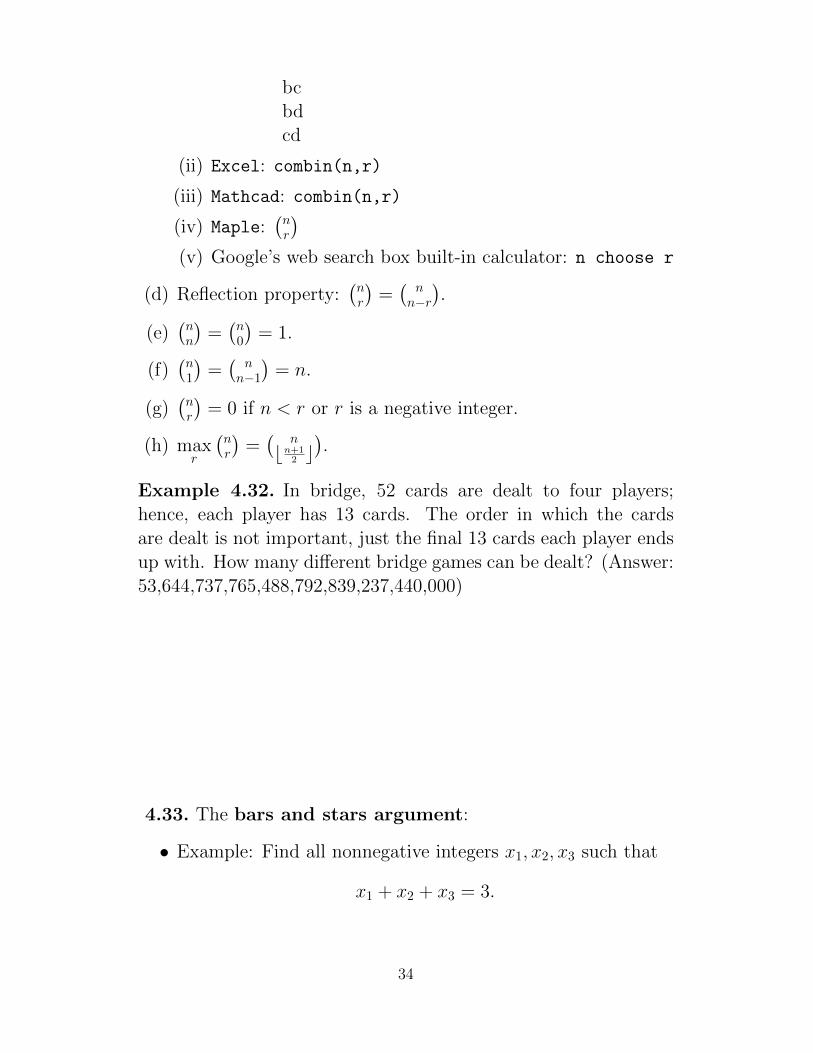
Example 4.32. In bridge, 52 cards are dealt to four players;hence, each player has 13 cards. The order in which the cardsare dealt is not important, just the final 13 cards each player endsup with. How many different bridge games can be dealt? (Answer:53,644,737,765,488,792,839,237,440,000)
4.33. The bars and stars argument:
• Example: Find all nonnegative integers x1, x2, x3 such that
x1 + x2 + x3 = 3.
34

0 + 0 + 3 1 1 10 + 1 + 2 1 1 10 + 2 + 1 1 1 10 + 3 + 0 1 1 11 + 0 + 2 1 1 11 + 1 + 1 1 1 11 + 2 + 0 1 1 12 + 0 + 1 1 1 12 + 1 + 0 1 1 13 + 0 + 0 1 1 1
• There are(n+r−1
r
)=(n+r−1n−1
)distinct vector x = xn1 of non-
negative integers such that x1 + x2 + · · · + xn = r. We usen− 1 bars to separate r 1’s.
(a) Suppose we further require that the xi are strictly positive(xi ≥ 1), then there are
(r−1n−1
)solutions.
(b) Extra Lower-bound Requirement : Suppose we fur-ther require that xi ≥ ai where the ai are some givennonnegative integers, then the number of solution is(
r − (a1 + a2 + · · ·+ an) + n− 1
n− 1
).
Note that here we work with equivalent problem: y1 +y2 + · · ·+ yn = r −∑n
i=1 ai where yi ≥ 0.
• Consider the distribution of r = 10 indistinguishable ballsinto n = 5 distinguishable cells. Then, we only concern withthe number of balls in each cell. Using n − 1 = 4 bars, wecan divide r = 10 stars into n = 5 groups. For example,****|***||**|* would mean (4,3,0,2,1). In general, there are(n+r−1
r
)ways of arranging the bars and stars.
4.34. Unordered sampling with replacement : There aren items. We sample r out of these n items with replacement.Because the order in the sequences is not important in this kindof sampling, two samples are distinguished by the number of eachitem in the sequence. In particular, Suppose r letters are drawn
35

with replacement from a set a1, a2, . . . , an. Let xi be the numberof ai in the drawn sequence. Because we sample r times, we knowthat, for every sample, x1 + x2 + · · ·xn = r where the xi are non-negative integers. Hence, there are
(n+r−1
r
)possible unordered
samples with replacement.
4.3 Binomial Theorem and Multinomial Theorem
4.35. Binomial theorem : Sometimes, the number(nr
)is called
a binomial coefficient because it appears as the coefficient ofxryn−r in the expansion of the binomial (x+y)n. More specifically,for any positive integer n, we have,
(x+ y)n =n∑r=0
(n
r
)xryn−r (3)
(Slide) To see how we get (3), let’s consider a smaller case ofn = 3. The expansion of (x+y)3 can be found using combinatorialreasoning instead of multiplying the three terms out. When (x +y)3 = (x+y)(x+y)(x+y) is expanded, all products of a term in thefirst sum, a term in the second sum, and a term in the third sumare added. Terms of the form x3, x2y, xy2, and y3 arise. To obtaina term of the form x3, an x must be chosen in each of the sums,and this can be done in only one way. Thus, the x3 term in theproduct has a coefficient of 1. To obtain a term of the form x2y,an x must be chosen in two of the three sums (and consequentlya y in the other sum). Hence. the number of such terms is thenumber of 2-combinations of three objects, namely,
(32
). Similarly,
the number of terms of the form xy2 is the number of ways to pickone of the three sums to obtain an x (and consequently take a yfrom each of the other two terms). This can be done in
(31
)ways.
Finally, the only way to obtain a y3 term is to choose the y foreach of the three sums in the product, and this can be done inexactly one way. Consequently. it follows that
(x+ y)3 = x3 + 3x2y + 3xy2 + y3.
Now, let’s state a combinatorial proof of the binomial theorem(3). The terms in the product when it is expanded are of the form
36
xryn−r for r = 0, 1, 2, . . . , n. To count the number of terms of theform xryn−r, note that to obtain such a term it is necessary tochoose r xs from the n sums (so that the other n− r terms in theproduct are ys). Therefore. the coefficient of xryn−r is
(nr
).
From (3), if we let x = y = 1, then we get another importantidentity:
n∑r=0
(n
r
)= 2n. (4)
4.36. Multinomial Counting : The multinomial coefficient(n
n1 n2 · · · nr
)is defined as
r∏i=1
(n−
i−1∑k=0
nk
ni
)=
(n
n1
)·(n− n1
n2
)·(n− n1 − n2
n3
)· · ·(nrnr
)=
n!r∏i=1
ni!.
We have seen this before in (4.28). It is the number of ways that
we can arrange n =r∑i=1
ni tokens when having r types of symbols
and ni indistinguishable copies/tokens of a type i symbol.
4.37. Multinomial Theorem :
(x1 + . . .+ xr)n =
∑ n!
i1!i2! · · · ir!xi11 x
i22 · · ·xirr ,
where the sum ranges over all ordered r-tuples of integers i1, . . . , irsatisfying the following conditions:
i1 ≥ 0, . . . , ir ≥ 0, i1 + i2 + · · ·+ ir = n.
When r = 2 this reduces to the binomial theorem.
37

Sirindhorn International Institute of Technology
Thammasat University
School of Information, Computer and Communication Technology
ECS315 2013/1 Part I.3 Dr.Prapun4.38. Further reading on combinatorial ideas: the pigeon-hole
principle, inclusion-exclusion principle, generating functions andrecurrence relations, and flows in networks.
4.4 Famous Example: Galileo and the Duke of Tuscany
Example 4.39. When you toss three dice, the chance of the sumbeing 10 is greater than the chance of the sum being 9.
• The Grand Duke of Tuscany “ordered” Galileo to explain aparadox arising in the experiment of tossing three dice [2]:
“Why, although there were an equal number of 6 par-titions of the numbers 9 and 10, did experience statethat the chance of throwing a total 9 with three fairdice was less than that of throwing a total of 10?”
• Partitions of sums 11, 12, 9 and 10 of the game of three fairdice:
1+4+6=11 1+5+6=12 3+3+3=9 1+3+6=102+3+6=11 2+4+6=12 1+2+6=9 1+4+5=102+4+5=11 3+4+5=12 1+3+5=9 2+2+6=101+5+5=11 2+5+5=12 1+4+4=9 2+3+5=103+3+5=11 3+3+6=12 2+2+5=9 2+4+4=103+4+4=11 4+4+4=12 2+3+4=9 3+3+3=10
The partitions above are not equivalent. For example, fromthe addenda 1, 2, 6, the sum 9 can come up in 3! = 6 different
38

ways; from the addenda 2, 2, 5, the sum 9 can come up in3!
2!1! = 3 different ways; the sum 9 can come up in only oneway from 3, 3, 3.
• Remarks : Let Xi be the outcome of the ith dice and Sn bethe sum X1 +X2 + · · ·+Xn.
(a) P [S3 = 9] = P [S3 = 12] = 2563 < 27
63 = P [S3 = 10] =P [S3 = 11]. Note that the difference between the twoprobabilities is only 1
108 .
(b) The range of Sn is from n to 6n. So, there are 6n−n+1 =5n+ 1 possible values.
(c) The pmf of Sn is symmetric around its expected value atn+6n
2 = 7n2 .
P [Sn = m] = P [Sn = 7n−m].
0 5 10 15 20 250
0.02
0.04
0.06
0.08
0.1
0.12
0.14
n=3n=4
Figure 2: pmf of Sn for n = 3 and n = 4.
4.5 Application: Success Runs
Example 4.40. We are all familiar with “success runs” in manydifferent contexts. For example, we may be or follow a tennisplayer and count the number of consecutive times the player’s firstserve is good. Or we may consider a run of forehand winners. Abasketball player may be on a “hot streak” and hit his or hershots perfectly for a number of plays in row.
39

In all the examples, whether you should or should not be amazedby the observation depends on a lot of other information. Theremay be perfectly reasonable explanations for any particular successrun. But we should be curious as to whether randomness couldalso be a perfectly reasonable explanation. Could the hot streakof a player simply be a snapshot of a random process, one that weparticularly like and therefore pay attention to?
In 1985, cognitive psychologists Amos Taversky and ThomasGilovich examined12 the shooting performance of the Philadelphia76ers, Boston Celtics and Cornell University’s men’s basketballteam. They sought to discover whether a player’s previous shothad any predictive effect on his or her next shot. Despite basketballfans’ and players’ widespread belief in hot streaks, the researchersfound no support for the concept. (No evidence of nonrandombehavior.) [14, p 178]
4.41. Academics call the mistaken impression that a randomstreak is due to extraordinary performance the hot-hand fallacy.Much of the work on the hot-hand fallacy has been done in thecontext of sports because in sports, performance is easy to defineand measure. Also, the rules of the game are clear and definite,data are plentiful and public, and situations of interest are repli-cated repeatedly. Not to mention that the subject gives academicsa way to attend games and pretend they are working. [14, p 178]
Example 4.42. Suppose that two people are separately asked totoss a fair coin 120 times and take note of the results. Heads isnoted as a “one” and tails as a “zero”. The following two lists ofcompiled zeros and ones result
1 1 0 0 1 0 0 1 0 1 1 0 0 1 0 0 0 1 1 0 1 0 1 0 0 1 1 0 1 00 1 0 1 0 1 1 0 1 1 0 0 1 1 0 1 1 1 0 1 0 0 1 0 0 1 1 0 1 00 1 1 0 1 0 0 1 1 0 1 0 1 1 0 0 1 1 1 0 0 1 0 1 0 1 0 0 0 10 1 0 1 0 1 0 1 0 1 1 0 0 1 0 0 1 0 1 1 0 0 1 0 0 1 1 0 1 1
and12“The Hot Hand in Basketball: On the Misperception of Random Sequences”
40

1 1 1 0 0 0 1 1 1 0 1 0 1 1 1 1 1 1 0 1 0 0 0 1 1 0 0 1 1 01 0 1 0 0 0 1 1 0 1 0 0 1 1 1 0 1 0 0 0 0 1 0 1 1 1 0 1 1 00 1 1 1 0 1 1 0 0 1 1 1 1 1 1 0 1 1 0 1 0 1 1 1 0 0 0 0 0 00 0 1 1 0 1 1 1 0 1 1 1 1 0 1 1 1 1 0 1 0 1 1 0 1 1 0 1 0 1
One of the two individuals has cheated and has fabricated a list ofnumbers without having tossed the coin. Which list is more likelybe the fabricated list? [21, Ex. 7.1 p 42–43]
The answer is later provided in Example 4.48.
Definition 4.43. A run is a sequence of more than one consecu-tive identical outcomes, also known as a clump.
Definition 4.44. Let Rn represent the length of the longest runof heads in n independent tosses of a fair coin. Let An(x) be theset of (head/tail) sequences of length n in which the longest runof heads does not exceed x. Let an(x) = ‖An(x)‖.Example 4.45. If a fair coin is flipped, say, three times, we caneasily list all possible sequences:
HHH, HHT, HTH, HTT, THH, THT, TTH, TTT
and accordingly derive:
x P [R3 = x] a3(x)
0 1/8 11 4/8 42 2/8 73 1/8 8
4.46. Consider an(x). Note that if n ≤ x, then an(x) = 2n becauseany outcome is a favorable one. (It is impossible to get more thanthree heads in three coin tosses). For n > x, we can partitionAn(x) by the position k of the first tail. Observe that k must be≤ x + 1 otherwise we will have more than x consecutive heads inthe sequence which contradicts the definition of An(x). For eachk ∈ 1, 2, . . . , x+ 1, the favorable sequences are in the form
HH . . . H︸ ︷︷ ︸k−1 heads
T XX . . .X︸ ︷︷ ︸n−k positions
41

where, to keep the sequences in An(x), the last n − k positions13
must be in An−k(x). Thus,
an(x) =x+1∑k=1
an−k(x) for n > x.
In conclusion, we have
an(x) =
∑xj=0 an−j−1(x), n > x,
2n n ≤ x
[20]. The following MATLAB function calculates an(x)
function a = a nx(n,x)a = [2.ˆ(1:x) zeros(1,n−x)];a(x+1) = 1+sum(a(1:x));for k = (x+2):n
a(k) = sum(a((k−1−x):(k−1)));enda = a(n);
4.47. Similar technique can be used to contract Bn(x) defined asthe set of sequences of length n in which the longest run of headsand the longest run of tails do not exceed x. To check whethera sequence is in Bn(x), first we convert it into sequence of S andD by checking each adjacent pair of coin tosses in the originalsequence. S means the pair have same outcome and D means theyare different. This process gives a sequence of length n−1. Observethat a string of x−1 consecutive S’s is equivalent to a run of lengthx. This put us back to the earlier problem of finding an(x) wherethe roles of H and T are now played by S and D, respectively. (Thelength of the sequence changes from n to n − 1 and the max runlength is x − 1 for S instead of x for H.) Hence, bn(x) = ‖Bn(x)‖can be found by
bn(x) = 2an−1(x− 1)
[20].
13Strictly speaking, we need to consider the case when n = x+ 1 separately. In such case,when k = x+ 1, we have A0(x). This is because the sequence starts with x heads, then a tail,and no more space left. In which case, this part of the partition has only one element; so weshould define a0(x) = 1. Fortunately, for x ≥ 1, this is automatically satisfied in an(x) = 2n.
42

Example 4.48. Continue from Example 4.42. We can check thatin 120 tosses of a fair coin, there is a very large probability that atsome point during the tossing process, a sequence of five or moreheads or five or more tails will naturally occur. The probability ofthis is
2120 − b120(4)
2120≈ 0.9865.
0.9865. In contrast to the second list, the first list shows no suchsequence of five heads in a row or five tails in a row. In the firstlist, the longest sequence of either heads or tails consists of threein a row. In 120 tosses of a fair coin, the probability of the longestsequence consisting of three or less in a row is equal to
b120(3)
2120≈ 0.000053,
which is extremely small indeed. Thus, the first list is almostcertainly a fake. Most people tend to avoid noting long sequencesof consecutive heads or tails. Truly random sequences do not sharethis human tendency! [21, Ex. 7.1 p 42–43]
43
Sirindhorn International Institute of Technology
Thammasat University
School of Information, Computer and Communication Technology
ECS315 2013/1 Part II Dr.Prapun
5 Probability Foundations
Constructing the mathematical foundations of probability theoryhas proven to be a long-lasting process of trial and error. Theapproach consisting of defining probabilities as relative frequenciesin cases of repeatable experiments leads to an unsatisfactory theory.The frequency view of probability has a long history that goesback to Aristotle. It was not until 1933 that the great Russianmathematician A. N. Kolmogorov (1903-1987) laid a satisfactorymathematical foundation of probability theory. He did this bytaking a number of axioms as his starting point, as had been donein other fields of mathematics. [21, p 223]
We will try to avoid several technical details14 15 in this class.Therefore, the definition given below is not the “complete” defini-tion. Some parts are modified or omitted to make the definitioneasier to understand.
14To study formal definition of probability, we start with the probability space (Ω,A, P ).Let Ω be an arbitrary space or set of points ω. Recall (from Definition 1.15) that, viewedprobabilistically, a subset of Ω is an event and an element ω of Ω is a sample point . Eachevent is a collection of outcomes which are elements of the sample space Ω.
The theory of probability focuses on collections of events, called event σ-algebras, typ-ically denoted by A (or F), that contain all the events of interest (regarding the randomexperiment E) to us, and are such that we have knowledge of their likelihood of occurrence.The probability P itself is defined as a number in the range [0, 1] associated with each eventin A.
15The class 2Ω of all subsets can be too large for us to define probability measures withconsistency, across all member of the class. (There is no problem when Ω is countable.)
44

Definition 5.1. Kolmogorov’s Axioms for Probability [12]:A probability measure16 is a real-valued set function17 that sat-isfies
P1 Nonnegativity :P (A) ≥ 0.
P2 Unit normalization :
P (Ω) = 1.
P3 Countable additivity or σ-additivity : For every countablesequence (An)
∞n=1 of disjoint events,
P
( ∞⋃n=1
An
)=
∞∑n=1
P (An).
• The number P (A) is called the probability of the event A
• The entire sample space Ω is called the sure event or thecertain event.
• If an event A satisfies P (A) = 1, we say that A is an almost-sure event.
• A support of P is any set A for which P (A) = 1.
From the three axioms18, we can derive many more propertiesof probability measure. These properties are useful for calculatingprobabilities.
16Technically, probability measure is defined on a σ-algebra A of Ω. The triple (Ω,A, P ) iscalled a probability measure space , or simply a probability space
17A real-valued set function is a function the maps sets to real numbers.18Remark: The axioms do not determine probabilities; the probabilities are assigned based
on our knowledge of the system under study. (For example, one approach is to base probabilityassignments on the simple concept of equally likely outcomes.) The axioms enable us to easilycalculate the probabilities of some events from knowledge of the probabilities of other events.
45

5.2. P (∅) = 0.
5.3. Finite additivity19: If A1, . . . , An are disjoint events, then
P
(n⋃i=1
Ai
)=
n∑i=1
P (Ai).
Special case when n = 2: Addition rule (Additivity)
If A ∩B = ∅, then P (A ∪B) = P (A) + P (B). (5)
19It is not possible to go backwards and use finite additivity to derive countable additivity(P3).
46
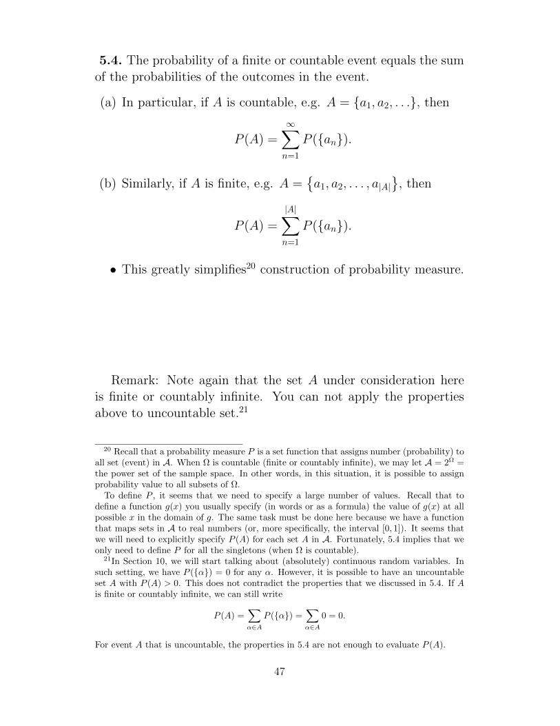
5.4. The probability of a finite or countable event equals the sumof the probabilities of the outcomes in the event.
(a) In particular, if A is countable, e.g. A = a1, a2, . . ., then
P (A) =∞∑n=1
P (an).
(b) Similarly, if A is finite, e.g. A =a1, a2, . . . , a|A|
, then
P (A) =
|A|∑n=1
P (an).
• This greatly simplifies20 construction of probability measure.
Remark: Note again that the set A under consideration hereis finite or countably infinite. You can not apply the propertiesabove to uncountable set.21
20 Recall that a probability measure P is a set function that assigns number (probability) toall set (event) in A. When Ω is countable (finite or countably infinite), we may let A = 2Ω =the power set of the sample space. In other words, in this situation, it is possible to assignprobability value to all subsets of Ω.
To define P , it seems that we need to specify a large number of values. Recall that todefine a function g(x) you usually specify (in words or as a formula) the value of g(x) at allpossible x in the domain of g. The same task must be done here because we have a functionthat maps sets in A to real numbers (or, more specifically, the interval [0, 1]). It seems thatwe will need to explicitly specify P (A) for each set A in A. Fortunately, 5.4 implies that weonly need to define P for all the singletons (when Ω is countable).
21In Section 10, we will start talking about (absolutely) continuous random variables. Insuch setting, we have P (α) = 0 for any α. However, it is possible to have an uncountableset A with P (A) > 0. This does not contradict the properties that we discussed in 5.4. If Ais finite or countably infinite, we can still write
P (A) =∑α∈A
P (α) =∑α∈A
0 = 0.
For event A that is uncountable, the properties in 5.4 are not enough to evaluate P (A).
47
Example 5.5. A random experiment can result in one of the out-comes a, b, c, d with probabilities 0.1, 0.3, 0.5, and 0.1, respec-tively. Let A denote the event a, b, B the event b, c, d, and Cthe event d.
• P (A) =
• P (B) =
• P (C) =
• P (Ac) =
• P (A ∩B) =
• P (A ∩ C) =
5.6. Monotonicity : If A ⊂ B, then P (A) ≤ P (B)
Example 5.7. Let A be the event to roll a 6 and B the eventto roll an even number. Whenever A occurs, B must also occur.However, B can occur without A occurring if you roll 2 or 4.
5.8. If A ⊂ B, then P (B \ A) = P (B)− P (A)
5.9. P (A) ∈ [0, 1].
5.10. P (A∩B) can not exceed P (A) and P (B). In other words,“the composition of two events is always less probable than (or atmost equally probable to) each individual event.”
48

Example 5.11 (Slides). Experiments by psychologists Kahnemanand Tversky.
Example 5.12. Let us consider Mrs. Boudreaux and Mrs. Thi-bodeaux who are chatting over their fence when the new neighborwalks by. He is a man in his sixties with shabby clothes and adistinct smell of cheap whiskey. Mrs.B, who has seen him before,tells Mrs. T that he is a former Louisiana state senator. Mrs. Tfinds this very hard to believe. “Yes,” says Mrs.B, “he is a formerstate senator who got into a scandal long ago, had to resign, andstarted drinking.” “Oh,” says Mrs. T, “that sounds more likely.”“No,” says Mrs. B, “I think you mean less likely.”
Strictly speaking, Mrs. B is right. Consider the following twostatements about the shabby man: “He is a former state senator”and “He is a former state senator who got into a scandal long ago,had to resign, and started drinking.” It is tempting to think thatthe second is more likely because it gives a more exhaustive expla-nation of the situation at hand. However, this reason is preciselywhy it is a less likely statement. Note that whenever somebodysatisfies the second description, he must also satisfy the first butnot vice versa. Thus, the second statement has a lower probability(from Mrs. Ts subjective point of view; Mrs. B of course knowswho the man is).
This example is a variant of examples presented in the bookJudgment under Uncertainty [11] by Economics Nobel laureateDaniel Kahneman and co-authors Paul Slovic and Amos Tversky.They show empirically how people often make similar mistakeswhen they are asked to choose the most probable among a set ofstatements. It certainly helps to know the rules of probability. Amore discomforting aspect is that the more you explain somethingin detail, the more likely you are to be wrong. If you want to becredible, be vague. [17, p 11–12]
49
5.13. Complement Rule:
P (Ac) = 1− P (A) .
• “The probability that something does not occur can be com-puted as one minus the probability that it does occur.”
• Named “probability’s Trick Number One” in [10]
5.14. Probability of a union (not necessarily disjoint):
P (A ∪B) = P (A) + P (B)− P (A ∩B)
• P (A ∪B) ≤ P (A) + P (B).
• Approximation: If P (A) P (B) then we may approximateP (A ∪B) by P (A).
Example 5.15 (Slides). Combining error probabilities from vari-ous sources in DNA testing
Example 5.16. In his bestseller Innumeracy, John Allen Paulostells the story of how he once heard a local weatherman claim thatthere was a 50% chance of rain on Saturday and a 50% chance ofrain on Sunday and thus a 100% chance of rain during the weekend.Clearly absurd, but what is the error?
Answer: Faulty use of the addition rule (5)!If we let A denote the event that it rains on Saturday and B
the event that it rains on Sunday, in order to use P (A ∪ B) =P (A)+P (B), we must first confirm that A and B cannot occur at
50

the same time (P (A∩B) = 0). More generally, the formula that isalways holds regardless of whether P (A∩B) = 0 is given by 5.14:
P (A ∪B) = P (A) + P (B)− P (A ∩B).
The event “A∩B” describes the case in which it rains both days.To get the probability of rain over the weekend, we now add 50%and 50%, which gives 100%, but we must then subtract the prob-ability that it rains both days. Whatever this is, it is certainlymore than 0 so we end up with something less than 100%, just likecommon sense tells us that we should.
You may wonder what the weatherman would have said if thechances of rain had been 75% each day. [17, p 12]
5.17. Probability of a union of three events:
P (A ∪B ∪ C) = P (A) + P (B) + P (C)
− P (A ∩B)− P (A ∩ C)− P (B ∩ C)
+ P (A ∩B ∩ C)
5.18. Two bounds:
(a) Subadditivity or Boole’s Inequality: If A1, . . . , An areevents, not necessarily disjoint, then
P
(n⋃i=1
Ai
)≤
n∑i=1
P (Ai).
(b) σ-subadditivity or countable subadditivity: If A1, A2,. . . is a sequence of measurable sets, not necessarily disjoint,then
P
( ∞⋃i=1
Ai
)≤
∞∑i=1
P (Ai)
• This formula is known as the union bound in engineer-ing.
51
5.19. If a (finite) collection B1, B2, . . . , Bn is a partition of Ω,then
P (A) =n∑i=1
P (A ∩Bi)
Similarly, if a (countable) collection B1, B2, . . . is a partitionof Ω, then
P (A) =∞∑i=1
P (A ∩Bi)
5.20. Connection to classical probability theory: Consider anexperiment with finite sample space Ω = ω1, ω2, . . . , ωn in whicheach outcome ωi is equally likely. Note that n = |Ω|.
We must have
P (ωi) =1
n, ∀i.
Now, given any event finite22 event A, we can apply 5.4 to get
P (A) =∑ω∈A
P (ω) =∑ω∈A
1
n=|A|n
=|A||Ω| .
We can then say that the probability theory we are working onright now is an extension of the classical probability theory. Whenthe conditons/assumptions of classical probability theory are met,then we get back the defining definition of classical classical prob-ability. The extended part gives us ways to deal with situationwhere assumptions of classical probability theory are not satisfied.
22In classical probability, the sample space is finite; therefore, any event is also finite.
52

6 Event-based Independence and Conditional
Probability
Example 6.1. Roll a dice. . .Example
3
Roll a fair dice
Sneak peek:Figure 3: Conditional Probability Example: Sneak Peek
Example 6.2 (Slides). Diagnostic Tests.
6.1 Event-based Conditional Probability
Definition 6.3. Conditional Probability : The conditional prob-ability P (A|B) of event A, given that event B 6= ∅ occurred, isgiven by
P (A|B) =P (A ∩B)
P (B). (6)
• Some ways to say23 or express the conditional probability,P (A|B), are:
the “probability of A, given B”
the “probability of A, knowing B”
the “probability of A happening, knowing B has alreadyoccurred”
23Note also that although the symbol P (A|B) itself is practical, it phrasing in words can beso unwieldy that in practice, less formal descriptions are used. For example, we refer to “theprobability that a tested-positive person has the disease” instead of saying “the conditionalprobability that a randomly chosen person has the disease given that the test for this personreturns positive result.”
53

• Defined only when P (B) > 0.
If P (B) = 0, then it is illogical to speak of P (A|B); thatis P (A|B) is not defined.
6.4. Interpretation : Sometimes, we refer to P (A) as
• a priori probability , or
• the prior probability of A, or
• the unconditional probability of A.
It is sometimes useful to interpret P (A) as our knowledge ofthe occurrence of event A before the experiment takes place. Con-ditional probability P (A|B) is the updated probability of theevent A given that we now know that B occurred (but we still donot know which particular outcome in the set B occurred).
Example 6.5. Back to Example 6.1
Example
3
Roll a fair dice
Sneak peek:Figure 4: Sneak Peek: A Revisit
54

Example 6.6. In diagnostic tests Example 6.2, we learn whetherwe have the disease from test result. Originally, before taking thetest, the probability of having the disease is 0.01%. Being testedpositive from the 99%-accurate test updates the probability ofhaving the disease to about 1%.
More specifically, let D be the event that the testee has thedisease and TP be the event that the test returns positive result.
• Before taking the test, the probability of having the diseaseis P (D) = 0.01%.
• Using 99%-accurate test means
P (TP |D) = 0.99 and P (T cP |Dc) = 0.99.
• Our calculation shows that P (D|TP ) ≈ 0.01.
6.7. “Prelude” to the concept of “independence”:If the occurrence of B does not give you more information aboutA, then
P (A|B) = P (A) (7)
and we say that A and B are independent .
• Meaning: “learning that eventB has occurred does not changethe probability that event A occurs.”
We will soon define “independence” in Section 6.2. Property(7) can be regarded as a “practical” definition for independence.However, there are some “technical” issues24 that we need to dealwith when we actually define independence.
24Here, the statement assume P (B) > 0 because it considers P (A|B). The concept ofindependence to be defined in Section 6.2 will not rely directly on conditional probability andtherefore it will include the case where P (B) = 0.
55

6.8. Similar properties to the three probability axioms:
(a) Nonnegativity: P (A|B) ≥ 0
(b) Unit normalization: P (Ω|B) = 1.
In fact, for any event A such that B ⊂ A, we have P (A|B) =1.
This impliesP (Ω|B) = P (B|B) = 1.
(c) Countable additivity: For every countable sequence (An)∞n=1
of disjoint events,
P
( ∞⋃n=1
An
∣∣∣∣∣B)
=∞∑n=1
P (An|B).
• In particular, if A1 ⊥ A2,
P (A1 ∪ A2 |B ) = P (A1 |B ) + P (A2 |B )
6.9. More Properties:
• P (A|Ω) = P (A)
• P (Ac|B) = 1− P (A|B)
• P (A ∩B|B) = P (A|B)
• P (A1 ∪ A2|B) = P (A1|B) + P (A2|B)− P (A1 ∩ A2|B).
• P (A ∩B) ≤ P (A|B)
56

6.10. When Ω is finite and all outcomes have equal probabilities,
P (A|B) =P (A ∩B)
P (B)=|A ∩B| / |Ω||B| / |Ω| =
|A ∩B||B| .
This formula can be regarded as the classical version of conditionalprobability.
Example 6.11. Someone has rolled a fair dice twice. You knowthat one of the rolls turned up a face value of six. The probabilitythat the other roll turned up a six as well is 1
11 (not 16). [21,
Example 8.1, p. 244]
6.12. Probability of compound events
(a) P (A ∩B) = P (A)P (B|A)
(b) P (A ∩B ∩ C) = P (A ∩B)× P (C|A ∩B)
(c) P (A ∩B ∩ C) = P (A)× P (B|A)× P (C|A ∩B)
When we have many sets intersected in the conditioned part, weoften use “,” instead of “∩”.
Example 6.13. Most people reason as follows to find the proba-bility of getting two aces when two cards are selected at randomfrom an ordinary deck of cards:
(a) The probability of getting an ace on the first card is 4/52.
(b) Given that one ace is gone from the deck, the probability ofgetting an ace on the second card is 3/51.
(c) The desired probability is therefore
4
52× 3
51.
[21, p 243]
Question: What about the unconditional probability P (B)?
57

Example 6.14. You know that roughly 5% of all used cars havebeen flood-damaged and estimate that 80% of such cars will laterdevelop serious engine problems, whereas only 10% of used carsthat are not flood-damaged develop the same problems. Of course,no used car dealer worth his salt would let you know whether yourcar has been flood damaged, so you must resort to probabilitycalculations. What is the probability that your car will later runinto trouble?
You might think about this problem in terms of proportions.
If you solved the problem in this way, congratulations. Youhave just used the law of total probability.
6.15. Total Probability Theorem : If a (finite or infinitely)countable collection of events B1, B2, . . . is a partition of Ω, then
P (A) =∑i
P (A|Bi)P (Bi). (8)
This is a formula25 for computing the probability of an eventthat can occur in different ways.
6.16. Special case:
P (A) = P (A|B)P (B) + P (A|Bc)P (Bc).
This gives exactly the same calculation as what we discussed inExample 6.14.
25The tree diagram is useful for helping you understand the process. However, then thenumber of possible cases is large (many Bi for the partition), drawing the tree diagram maybe too time-consuming and therefore you should also learn how to apply the total probabilitytheorem directly without the help of the tree diagram.
58
Example 6.17. Continue from the “Diagnostic Tests” Example6.2 and Example 6.6.
P (TP ) = P (TP ∩D) + P (TP ∩Dc)
= P (TP |D)P (D) + P (TP |Dc )P (Dc) .
For conciseness, we define
pd = P (D)
andpTE = P (TP |Dc) = P (T cP |D).
Then,P (TP ) = (1− pTE)pD + pTE(1− pD).
6.18. Bayes’ Theorem:
(a) Form 1:
P (B|A) = P (A|B)P (B)
P (A).
(b) Form 2: If a (finite or infinitely) countable collection of eventsB1, B2, . . . is a partition of Ω, then
P (Bk|A) = P (A|Bk)P (Bk)
P (A)=
P (A|Bk)P (Bk)∑i P (A|Bi)P (Bi)
.
• Extremely useful for making inferences about phenomena thatcannot be observed directly.
• Sometimes, these inferences are described as “reasoning aboutcauses when we observe effects”.
59

Example 6.19. Continue from the “Disease Testing” Examples6.2, 6.6, and 6.17:
P (D |TP ) =P (D ∩ TP )
P (TP )=P (TP |D )P (D)
P (TP )
=(1− pTE)pD
(1− pTE)pD + pTE(1− pD)Effect of pTE
1
pTE = 1 – 0.99 = 0.01
0 0.1 0.2 0.3 0.4 0.5 0.6 0.7 0.8 0.9 10
0.1
0.2
0.3
0.4
0.5
0.6
0.7
0.8
0.9
1
pTE = 1 – 0.9 = 0.1
pTE = 1 – 0.5 = 0.5
pD
P(D|TP)
Figure 5: Probability P (D |TP ) that a person will have the disease given thatthe test result is positive. The conditional probability is evaluated as a func-tion of PD which tells how common the disease is. Thee values of test errorprobability pTE are shown.
Example 6.20. Medical Diagnostic: Because a new medical pro-cedure has been shown to be effective in the early detection of anillness, a medical screening of the population is proposed. Theprobability that the test correctly identifies someone with the ill-ness as positive is 0.99, and the probability that the test correctlyidentifies someone without the illness as negative is 0.95. The in-cidence of the illness in the general population is 0.0001. You takethe test, and the result is positive. What is the probability thatyou have the illness? [15, Ex. 2-37]
60

Example 6.21. Bayesian networks are used on the Web sites ofhigh-technology manufacturers to allow customers to quickly di-agnose problems with products. An oversimplified example is pre-sented here.
A printer manufacturer obtained the following probabilities froma database of test results. Printer failures are associated with threetypes of problems: hardware, software, and other (such as connec-tors), with probabilities 0.1, 0.6, and 0.3, respectively. The prob-ability of a printer failure given a hardware problem is 0.9, givena software problem is 0.2, and given any other type of problem is0.5. If a customer enters the manufacturers Web site to diagnosea printer failure, what is the most likely cause of the problem?
Let the events H, S, and O denote a hardware, software, orother problem, respectively, and let F denote a printer failure.
Example 6.22 (Slides). Prosecutor’s Fallacy and the Murder ofNicole Brown
6.23. In practice, here is how we use the total probability theoremand Bayes’ theorem:
Usually, we work with a system, which of course has input andoutput. There can be many possibilities for inputs and there can bemany possibilities for output. Normally, for deterministic system,we may have a specification that tells what would be the outputgiven that a specific input is used. Intuitively, we may think of this
61
as a table of mapping between input and output. For system withrandom component(s), when a specific input is used, the output isnot unique. This mean we needs conditional probability to describethe output (given an input). Of course, this conditional probabilitycan be different for different inputs.
We will assume that there are many cases that the input canhappen. The event that the ith case happens is denoted by Bi. Weassume that we consider all possible cases. Therefore, the unionof these Bi will automatically be Ω. If we also define the cases sothat they do not overlap, then the Bi partitions Ω.
Similarly, there are many cases that the output can happen.The event that the jth case happens is depenoted by Aj. Weassume that the Aj also partitions Ω.
In this way, the system itself can be described by the condi-tional probabilities of the form P (Aj|Bi). This replace the tablementioned above as the specification of the system. Note thateven when this information is not available, we can still obtain anapproximation of the conditional probability by repeating trials ofinputting Bi in to the system to find the relative frequency of theoutput Aj.
Now, when the system is used in actual situation. Differentinput cases can happen with different probabilities. These aredescribed by the prior probabilities P (Bi). Combining this withthe conditional probabilities P (Aj|Bi) above, we can use the totalprobability theorem to find the probability of occurrence for out-put and, even more importantly, for someone who cannot directlyobserve the input, Bayes’ theorem can be used to infer the value(or the probability) of the input from the observed output of thesystem.
In particular, total probability theorem deals with the calcula-tion of the output probabilities P (Aj):
P (Aj) =∑i
P (Aj ∩Bi) =∑i
P (Aj |Bi )P (Bi).
Bayes’ theorem calculates the probability that Bk was the inputevent when the observer can only observe the output of the system
62
and the observed value of the output is Aj:
P (Bk |Aj ) =P (Aj ∩Bk)
P (Aj)=
P (Aj |Bk )P (Bk)∑i
P (Aj |Bi )P (Bi).
Example 6.24. In the early 1990s, a leading Swedish tabloidtried to create an uproar with the headline “Your ticket is thrownaway!”. This was in reference to the popular Swedish TV show“Bingolotto” where people bought lottery tickets and mailed themto the show. The host then, in live broadcast, drew one ticket froma large mailbag and announced a winner. Some observant reporternoticed that the bag contained only a small fraction of the hun-dreds of thousands tickets that were mailed. Thus the conclusion:Your ticket has most likely been thrown away!
Let us solve this quickly. Just to have some numbers, let ussay that there are a total of N = 100, 000 tickets and that n =1, 000 of them are chosen at random to be in the final drawing.If the drawing was from all tickets, your chance to win wouldbe 1/N = 1/100, 000. The way it is actually done, you need toboth survive the first drawing to get your ticket into the bag andthen get your ticket drawn from the bag. The probability to getyour entry into the bag is n/N = 1, 000/100, 000. The conditionalprobability to be drawn from the bag, given that your entry is init, is 1/n = 1/1, 000. Multiply to get 1/N = 1/100, 000 once more.There were no riots in the streets. [17, p 22]
6.25. Chain rule of conditional probability [9, p 58]:
P (A ∩B|C) = P (B|C)P (A|B ∩ C).
Example 6.26. Your teacher tells the class there will be a surpriseexam next week. On one day, Monday-Friday, you will be told inthe morning that an exam is to be given on that day. You quicklyrealize that the exam will not be given on Friday; if it was, it wouldnot be a surprise because it is the last possible day to get theexam. Thus, Friday is ruled out, which leaves Monday-Thursday.But then Thursday is impossible also, now having become the lastpossible day to get the exam. Thursday is ruled out, but then
63

Wednesday becomes impossible, then Tuesday, then Monday, andyou conclude: There is no such thing as a surprise exam! But theteacher decides to give the exam on Tuesday, and come Tuesdaymorning, you are surprised indeed.
This problem, which is often also formulated in terms of sur-prise fire drills or surprise executions, is known by many names, forexample, the “hangman’s paradox” or by serious philosophers asthe “prediction paradox.” To resolve it, let’s treat it as a probabil-ity problem. Suppose that the day of the exam is chosen randomlyamong the five days of the week. Now start a new school week.What is the probability that you get the test on Monday? Obvi-ously 1/5 because this is the probability that Monday is chosen.If the test was not given on Monday. what is the probability thatit is given on Tuesday? The probability that Tuesday is chosento start with is 1/5, but we are now asking for the conditionalprobability that the test is given on Tuesday, given that it was notgiven on Monday. As there are now four days left, this conditionalprobability is 1/4. Similarly, the conditional probabilities that thetest is given on Wednesday, Thursday, and Friday conditioned onthat it has not been given thus far are 1/3, 1/2, and 1, respectively.
We could define the “surprise index” each day as the probabilitythat the test is not given. On Monday, the surprise index is there-fore 0.8, on Tuesday it has gone down to 0.75, and it continues togo down as the week proceeds with no test given. On Friday, thesurprise index is 0, indicating absolute certainty that the test willbe given that day. Thus, it is possible to give a surprise test butnot in a way so that you are equally surprised each day, and it isnever possible to give it so that you are surprised on Friday. [17,p 23–24]
Example 6.27. Today Bayesian analysis is widely employed through-out science and industry. For instance, models employed to deter-mine car insurance rates include a mathematical function describ-ing, per unit of driving time, your personal probability of havingzero, one, or more accidents. Consider, for our purposes, a sim-plified model that places everyone in one of two categories: highrisk, which includes drivers who average at least one accident each
64

year, and low risk, which includes drivers who average less thanone.
If, when you apply for insurance, you have a driving recordthat stretches back twenty years without an accident or one thatgoes back twenty years with thirty-seven accidents, the insurancecompany can be pretty sure which category to place you in. But ifyou are a new driver, should you be classified as low risk (a kid whoobeys the speed limit and volunteers to be the designated driver)or high risk (a kid who races down Main Street swigging from ahalf-empty $2 bottle of Boone’s Farm apple wine)?
Since the company has no data on you, it might assign youan equal prior probability of being in either group, or it mightuse what it knows about the general population of new driversand start you off by guessing that the chances you are a high riskare, say, 1 in 3. In that case the company would model you as ahybrid–one-third high risk and two-thirds low risk–and charge youone-third the price it charges high-risk drivers plus two-thirds theprice it charges low-risk drivers.
Then, after a year of observation, the company can employ thenew datum to reevaluate its model, adjust the one-third and two-third proportions it previously assigned, and recalculate what itought to charge. If you have had no accidents, the proportion oflow risk and low price it assigns you will increase; if you have hadtwo accidents, it will decrease. The precise size of the adjustmentis given by Bayes’s theory. In the same manner the insurancecompany can periodically adjust its assessments in later years toreflect the fact that you were accident-free or that you twice hadan accident while driving the wrong way down a one-way street,holding a cell phone with your left hand and a doughnut withyour right. That is why insurance companies can give out “gooddriver” discounts: the absence of accidents elevates the posteriorprobability that a driver belongs in a low-risk group. [14, p 111-112]
65
6.2 Event-based Independence
Plenty of random things happen in the world all the time, most ofwhich have nothing to do with one another. If you toss a coin andI roll a dice, the probability that you get heads is 1/2 regardless ofthe outcome of my dice. Events that are unrelated to each otherin this way are called independent.
Definition 6.28. Two events A, B are called (statistically26)independent if
P (A ∩B) = P (A)P (B) (9)
• Notation: A |= B• Read “A and B are independent” or “A is independent of B”
• We call (9) the multiplication rule for probabilities.
• If two events are not independent, they are dependent. In-tuitively, if two events are dependent, the probability of onechanges with the knowledge of whether the other has oc-curred.
6.29. Intuition: Again, here is how you should think about inde-pendent events: “If one event has occurred, the probability of theother does not change.”
P (A|B) = P (A) and P (B|A) = P (B). (10)
In other words, “the unconditional and the conditional probabili-ties are the same”. We can almost use (10) as the definitions forindependence. This is what we mentioned in 6.7. However, we use(9) instead because it (1) also works with events whose probabili-ties are zero and (2) also has clear symmetry in the expression (sothat A |= B and B |= A can clearly be seen as the same). In fact,in 6.33, we show how (10) can be used to define independence withextra condition that deals with the case when zero probability isinvolved.
26Sometimes our definition for independence above does not agree with the everyday-language use of the word “independence”. Hence, many authors use the term “statisticallyindependence” to distinguish it from other definitions.
66

Example 6.30. [25, Ex. 5.4] Which of the following pairs of eventsare independent?
(a) The card is a club, and the card is black.
Example: Club & Black
1
spades
clubs
hearts
diamonds
Figure 6: A Deck of Cards
(b) The card is a king, and the card is black.
6.31. An event with probability 0 or 1 is independent of any event(including itself).
• In particular, ∅ and Ω are independent of any events.
6.32. An event A is independent of itself if and only if P (A) is 0or 1.
6.33. Two events A, B with positive probabilities are independentif and only if P (B |A) = P (B), which is equivalent to P (A |B ) =P (A).
When A and/or B has zero probability, A and B are automat-ically independent.
6.34. When A and B have nonzero probabilities, the followingstatements are equivalent:
67

6.35. The following four statements are equivalent:
A |= B, A |= Bc, Ac |= B, Ac |= Bc.
Example 6.36. If P (A|B) = 0.4, P (B) = 0.8, and P (A) = 0.5,are the events A and B independent? [15]
6.37. Keep in mind that independent and disjoint are notsynonyms. In some contexts these words can have similar mean-ings, but this is not the case in probability.
• If two events cannot occur at the same time (they are disjoint),are they independent? At first you might think so. After all,they have nothing to do with each other, right? Wrong! Theyhave a lot to do with each other. If one has occurred, we knowfor certain that the other cannot occur. [17, p 12]
• To check whether A and B are disjoint, you only need tolook at the sets themselves and see whether they have sharedelement(s). This can be answered without knowing probabil-ities.
To check whether A and B are independent, you need to lookat the probabilities P (A), P (B), and P (A ∩B).
• Reminder: If events A and B are disjoint, you calculate theprobability of the union A ∪ B by adding the probabilitiesof A and B. For independent events A and B you calculatethe probability of the intersection A ∩ B by multiplying theprobabilities of A and B.
68

• The two statements A ⊥ B and A |= B can occur simultane-ously only when P (A) = 0 and/or P (B) = 0.
Reverse is not true in general.
Example 6.38. Experiment of flipping a fair coin twice. Ω =HH,HT, TH, TT. Define event A to be the event that the firstflip gives a H; that is A = HH,HT. Event B is the event thatthe second flip gives a H; that is B = HH,TH. Note that eventhough the events A and B are not disjoint, they are independent.
Example 6.39 (Slides). Prosecutor’s fallacy : In 1999, a Britishjury convicted Sally Clark of murdering two of her children whohad died suddenly at the ages of 11 and 8 weeks, respectively.A pediatrician called in as an expert witness claimed that thechance of having two cases of infant sudden death syndrome, or“cot deaths,” in the same family was 1 in 73 million. There wasno physical or other evidence of murder, nor was there a motive.Most likely, the jury was so impressed with the seemingly astro-nomical odds against the incidents that they convicted. But wheredid the number come from? Data suggested that a baby born intoa family similar to the Clarks faced a 1 in 8,500 chance of dyinga cot death. Two cot deaths in the same family, it was argued,therefore had a probability of (1/8, 500)2 which is roughly equal to1/73,000.000.
Did you spot the error? I hope you did. The computationassumes that successive cot deaths in the same family are inde-pendent events. This assumption is clearly questionable, and evena person without any medical expertise might suspect that geneticfactors play a role. Indeed, it has been estimated that if thereis one cot death, the next child faces a much larger risk, perhaps
69

around 1/100. To find the probability of having two cot deaths inthe same family, we should thus use conditional probabilities andarrive at the computation 1/8, 500×1/100, which equals l/850,000.Now, this is still a small number and might not have made the ju-rors judge differently. But what does the probability 1/850,000have to do with Sallys guilt? Nothing! When her first child died,it was certified to have been from natural causes and there wasno suspicion of foul play. The probability that it would happenagain without foul play was 1/100, and if that number had beenpresented to the jury, Sally would not have had to spend threeyears in jail before the verdict was finally overturned and the ex-pert witness (certainly no expert in probability) found guilty of“serious professional misconduct.”
You may still ask the question what the probability 1/100 hasto do with Sallys guilt. Is this the probability that she is inno-cent? Not at all. That would mean that 99% of all mothers whoexperience two cot deaths are murderers! The number 1/100 issimply the probability of a second cot death, which only meansthat among all families who experience one cot death, about 1%will suffer through another. If probability arguments are used incourt cases, it is very important that all involved parties under-stand some basic probability. In Sallys case, nobody did.
References: [14, 118–119] and [17, 22–23].
Definition 6.40. Three events A1, A2, A3 are independent if andonly if
P (A1 ∩ A2) = P (A1)P (A2)
P (A1 ∩ A3) = P (A1)P (A3)
P (A2 ∩ A3) = P (A2)P (A3)
P (A1 ∩ A2 ∩ A3) = P (A1)P (A2)P (A3)
Remarks :
(a) When the first three equations hold, we say that the threeevents are pairwise independent.
(b) We may use the term “mutually independence” to furtheremphasize that we have “independence” instead of “pairwiseindependence”.
70

Definition 6.41. The events A1, A2, . . . , An are independent ifand only if for any subcollection Ai1, Ai2, . . . , Aik,
P (Ai1 ∩ Ai2 ∩ · · · ∩ Aik) = P (Ai1)× P (Ai2)× · · · × P (Ain) .
• Note that part of the requirement is that
P (A1 ∩ A2 ∩ · · · ∩ An) = P (A1)× P (A2)× · · · × P (An) .
Therefore, if someone tells us that the events A1, A2, . . . , An
are independent, then one of the properties that we can con-clude is that
P (A1 ∩ A2 ∩ · · · ∩ An) = P (A1)× P (A2)× · · · × P (An) .
• Equivalently, this is the same as the requirement that
P
⋂j∈J
Aj
=∏j∈J
P (Aj) ∀J ⊂ [n] and |J | ≥ 2
• Note that the case when j = 1 automatically holds. The casewhen j = 0 can be regarded as the ∅ event case, which is alsotrivially true.
6.42. Four events A,B,C,D are pairwise independent if andonly if they satisfy the following six conditions:
P (A ∩B) = P (A)P (B),
P (A ∩ C) = P (A)P (C),
P (A ∩D) = P (A)P (D),
P (B ∩ C) = P (B)P (C),
P (B ∩D) = P (B)P (D), and
P (C ∩D) = P (C)P (D).
They are independent if and only if they are pairwise independent(satisfy the six conditions above) and also satisfy the following fivemore conditions:
P (B ∩ C ∩D) = P (B)P (C)P (D),
P (A ∩ C ∩D) = P (A)P (C)P (D),
P (A ∩B ∩D) = P (A)P (B)P (D),
P (A ∩B ∩ C) = P (A)P (B)P (C), and
P (A ∩B ∩ C ∩D) = P (A)P (B)P (C)P (D).
71
6.3 Bernoulli Trials
Example 6.43. Consider the following random experiments
(a) Flip a coin 10 times. We are interested in the number of headsobtained.
(b) Of all bits transmitted through a digital transmission channel,10% are received in error. We are interested in the number ofbits in error in the next five bits transmitted.
(c) A multiple-choice test contains 10 questions, each with fourchoices, and you guess at each question. We are interested inthe number of questions answered correctly.
These examples illustrate that a general probability model thatincludes these experiments as particular cases would be very useful.
Example 6.44. Each of the random experiments in Example 6.43can be thought of as consisting of a series of repeated, randomtrials. In all cases, we are interested in the number of trials thatmeet a specified criterion. The outcome from each trial eithermeets the criterion or it does not; consequently, each trial can besummarized as resulting in either a success or a failure.
Definition 6.45. A Bernoulli trial involves performing an ex-periment once and noting whether a particular event A occurs.
The outcome of the Bernoulli trial is said to be
(a) a “success” if A occurs and
(b) a “failure” otherwise.
We may view the outcome of a single Bernoulli trial as the out-come of a toss of an unfair coin for which the probability of heads(success) is p = P (A) and the probability of tails (failure) is 1− p.
• The labeling (“success” and “failure”) is not meant to be lit-eral and sometimes has nothing to do with the everyday mean-ing of the words. We can just as well use A and B or 0 and1.
72

Example 6.46. Examples of Bernoulli trials: Flipping a coin,deciding to vote for candidate A or candidate B, giving birth toa boy or girl, buying or not buying a product, being cured or notbeing cured, even dying or living are examples of Bernoulli trials.
• Actions that have multiple outcomes can also be modeled asBernoulli trials if the question you are asking can be phrasedin a way that has a yes or no answer, such as “Did the diceland on the number 4?” or “Is there any ice left on the NorthPole?”
Definition 6.47. (Independent) Bernoulli Trials = a Bernoullitrial is repeated many times.
(a) It is usually assumed that the trials are independent. Thisimplies that the outcome from one trial has no effect on theoutcome to be obtained from any other trial.
(b) Furthermore, it is often reasonable to assume that the prob-ability of a success in each trial is constant.
An outcome of the complete experiment is a sequence of suc-cesses and failures which can be denoted by a sequence of onesand zeroes.
Example 6.48. If we toss unfair coin n times, we obtain thespace Ω = H,Tn consisting of 2n elements of the form (ω1, ω2, . . . , ωn)where ωi = H or T.
Example 6.49. What is the probability of two failures and threesuccesses in five Bernoulli trials with success probability p.
We observe that the outcomes with three successes in five trialsare 11100, 11010, 11001, 10110, 10101, 10011, 01110, 01101, 01011,and 00111. We note that the probability of each outcome is aproduct of five probabilities, each related to one Bernoulli trial.In outcomes with three successes, three of the probabilities are pand the other two are 1 − p. Therefore, each outcome with threesuccesses has probability (1− p)2p3. There are 10 of them. Hence,the total probability is 10(1− p)2p3
73

6.50. The probability of exactly n1 success in n = n0+n1 bernoullitrials is (
n
n1
)(1− p)n−n1pn1 =
(n
n0
)(1− p)n0pn−n0.
Example 6.51. At least one occurrence of a 1-in-n-chance eventin n repeated trials:
0 5 10 15 20 25 30 35 40 45 500
0.1
0.2
0.3
0.4
0.5
0.6
0.7
0.8
0.9
1
n
n Bernoulli trials
1
Assume success probability = 1/n
#successes 1P
#successes 1P
#successes 0P #successes 2P
#successes 3P
10.3679
e
11 0.6321
e
10.1839
2e
Figure 7: A 1-in-n-chance event in n repeated Bernoulli trials
Example 6.52. Digital communication over unreliable chan-nels : Consider a communication system below
74

Here, we consider a simple channel called binary symmetricchannel:
This channel can be described as a channel that introduces ran-dom bit errors with probability p.
A crude digital communication system would put binary infor-mation into the channel directly; the receiver then takes whatevervalue that shows up at the channel output as what the sendertransmitted. Such communication system would directly suffer biterror probability of p.
In situation where this error rate is not acceptable, error controltechniques are introduced to reduce the error rate in the deliveredinformation.
One method of reducing the error rate is to use error-correctingcodes:
A simple error-correcting code is the repetition code. Exam-ple of such code is described below:
(a) At the transmitter, the “encoder” box performs the followingtask:
(i) To send a 1, it will send 11111 through the channel.
(ii) To send a 0, it will send 00000 through the channel.
75

(b) When the five bits pass through the channel, it may be cor-rupted. Assume that the channel is binary symmetric andthat it acts on each of the bit independently.
(c) At the receiver, we (or more specifically, the decoder box) get5 bits, but some of the bits may be changed by the channel.
To determine what was sent from the transmitter, the receiverapply the majority rule : Among the 5 received bits,
(i) if #1 > #0, then it claims that “1” was transmitted,
(ii) if #0 > #1, then it claims that “0” was transmitted.
Error Control Coding
1
Repetition Code at Tx: Repeat the bit n times.
Channel: Binary Symmetric Channel (BSC) with bit error probability p.
Majority Vote at Rx
0 0.05 0.1 0.15 0.2 0.25 0.3 0.35 0.4 0.45 0.50
0.05
0.1
0.15
0.2
0.25
0.3
0.35
0.4
0.45
0.5
n = 15
n = 5
n = 1
n = 25
p
P
Figure 8: Bit error probability for a simple system that uses repetition codeat the transmitter (repeat each bit n times) and majority vote at the receiver.The channel is assumed to be binary symmetric with bit error probability p.
76

Exercise 6.53 (F2011). Kakashi and Gai are eternal rivals. Kakashiis a little stronger than Gai and hence for each time that they fight,the probability that Kakashi wins is 0.55. In a competition, theyfight n times (where n is odd). Assume that the results of the fightsare independent. The one who wins more will win the competition.
Suppose n = 3, what is the probability that Kakashi wins thecompetition.
77
Sirindhorn International Institute of Technology
Thammasat University
School of Information, Computer and Communication Technology
ECS315 2013/1 Part III.1 Dr.Prapun
7 Random variables
In performing a chance experiment, one is often not interestedin the particular outcome that occurs but in a specific numericalvalue associated with that outcome. In fact, for most applica-tions, measurements and observations are expressed as numericalquantities.
Example 7.1. Take this course and observe your grades.
7.2. The advantage of working with numerical quantities is thatwe can perform mathematical operations on them.
In the mathematics of probability, averages are called expecta-tions or expected values.
78

Definition 7.3. A real-valued function X(ω) defined for all pointsω in a sample space Ω is called a random variable (r.v. or RV)27.
• So, a random variable is a rule that assigns a numerical valueto each possible outcome of a chance experiment.
• Intuitively, a random variable is a variable that takes on itsvalues by chance.
• The convention is to use capital letters such as X, Y, Z todenote random variables.
Example 7.4. Roll a fair dice: Ω = 1, 2, 3, 4, 5, 6.
27The term “random variable” is a misnomer. Technically, if you look at the definitioncarefully, a random variable is a deterministic function; that is, it is not random and it is nota variable. [Toby Berger][25, p 254]
• As a function, it is simply a rule that maps points/outcomes ω in Ω to real numbers.
• It is also a deterministic function; nothing is random about the mapping/assignment.The randomness in the observed values is due to the underlying randomness of theargument of the function X, namely the experiment outcomes ω.
• In other words, the randomness in the observed value of X is induced by the underlyingrandom experiment, and hence we should be able to compute the probabilities of theobserved values in terms of the probabilities of the underlying outcomes.
79

Example 7.5 (Three Coin Tosses). Counting the number of headsin a sequence of three coin tosses.Three Coin Tosses
3
TTT,TTH,THT,THH,HTT,HTH,HHT,HHH
0, TTT
1, TTH,THT,HTT
2, THH,HTH,HHT
3, HHH
N
TTT
HHH
HTT
THT
TTH
HHT
HTH
HHT
Real number line 0 1 2 3 4
Example 7.6 (Sum of Two Dice). If S is the sum of the dotswhen rolling one fair dice twice, the random variable S assigns thenumerical value i+j to the outcome (i, j) of the chance experiment.
Example 7.7. Continue from Example 7.4,
(a) What is the probability that X = 4?
(b) What is the probability that Y = 4?
80

Definition 7.8. Events involving random variables:
• [some condition(s) on X] = the set of outcomes in Ω such thatX(ω) satisfies the conditions.
• [X ∈ B] = ω ∈ Ω : X(ω) ∈ B• [a ≤ X < b] = [X ∈ [a, b)] = ω ∈ Ω : a ≤ X(ω) < b• [X > a] = ω ∈ Ω : X(ω) > a• [X = x] = ω ∈ Ω : X(ω) = x We usually use the corresponding lowercase letter to de-
note
(a) a possible value (realization) of the random variable
(b) the value that the random variable takes on
(c) the running values for the random variable
All of the above items are sets of outcomes. They are all events!
Example 7.9. Continue from Examples 7.4 and 7.7,
(a) [X = 4] = ω : X(ω) = 4(b) [Y = 4] = ω : Y (ω) = 4 =
ω : (ω − 3)2 = 4
Definition 7.10. To avoid double use of brackets (round brack-ets over square brackets), we write P [X ∈ B] when we meansP ([X ∈ B]). Hence,
P [X ∈ B] = P ([X ∈ B]) = P (ω ∈ Ω : X(ω) ∈ B) .Similarly,
P [X < x] = P ([X < x]) = P (ω ∈ Ω : X(ω) < x) .Example 7.11. In Example 7.5 (Three Coin Tosses), if the coinis fair, thenP [N < 2] =
81

7.12. At a certain point in most probability courses, the samplespace is rarely mentioned anymore and we work directly with ran-dom variables. The sample space often “disappears” along withthe “(ω)” of X(ω) but they are really there in the background.
Definition 7.13. A set S is called a support of a random variableX if P [X ∈ S] = 1.
• To emphasize that S is a support of a particular variable X,we denote a support of X by SX .
• Practically, we define a support of a random variable X to bethe set of all the “possible” values of X.28
• For any random variable, the set R of all real numbers isalways a support; however, it is not that useful because it doesnot further limit the possible values of the random variable.
• Recall that a support of a probability measure P is any setA ⊂ Ω such that P (A) = 1.
Definition 7.14. The probability distribution is a descriptionof the probabilities associated with the random variable.
7.15. There are three types of of random variables. The first type,which will be discussed in Section 8, is called discrete randomvariable . To tell whether a random variable is discrete, one simpleway is to consider the “possible” values of the random variable.If it is limited to only a finite or countably infinite number ofpossibilities, then it is discrete. We will later discuss continuousrandom variables whose possible values can be anywhere insome intervals of real numbers.
28Later on, you will see that 1) a default support of a discrete random variable is the setof values where the pmf is strictly positive and 2) a default support of a continuous randomvariable is the set of values where the pdf is strictly positive.
82

8 Discrete Random Variables
Intuitively, to tell whether a random variable is discrete, we simplyconsider the possible values of the random variable. If the randomvariable is limited to only a finite or countably infinite number ofpossibilities, then it is discrete.
Example 8.1. Voice Lines: A voice communication system fora business contains 48 external lines. At a particular time, thesystem is observed, and some of the lines are being used. Let therandom variable X denote the number of lines in use. Then, Xcan assume any of the integer values 0 through 48. [15, Ex 3-1]
Definition 8.2. A random variable X is said to be a discreterandom variable if there exists a countable number of distinctreal numbers xk such that∑
k
P [X = xk] = 1. (11)
In other words, X is a discrete random variable if and only if Xhas a countable support.
Example 8.3. For the random variable N in Example 7.5 (ThreeCoin Tosses),
For the random variable S in Example 7.6 (Sum of Two Dice),
8.4. Although the support SX of a random variable X is defined asany set S such that P [X ∈ S] = 1. For discrete random variable,SX is usually set to be x : pX(x) > 0, the set of all “possiblevalues” of X.
Definition 8.5. Important Special Case: An integer-valued ran-dom variable is a discrete random variable whose xk in (11)above are all integers.
83

8.6. Recall, from 7.14, that the probability distribution of arandom variable X is a description of the probabilities associatedwith X.
For a discrete random variable, the distribution is often char-acterized by just a list of the possible values (x1, x2, x3, . . .) alongwith the probability of each:
(P [X = x1] , P [X = x2] , P [X = x3] , . . . , respectively) .
In some cases, it is convenient to express the probability interms of a formula. This is especially useful when dealing with arandom variable that has an unbounded number of outcomes. Itwould be tedious to list all the possible values and the correspond-ing probabilities.
8.1 PMF: Probability Mass Function
Definition 8.7. When X is a discrete random variable satisfying(11), we define its probability mass function (pmf) by29
pX(x) = P [X = x].
• Sometimes, when we only deal with one random variable orwhen it is clear which random variable the pmf is associatedwith, we write p(x) or px instead of pX(x).
• The argument (x) of a pmf ranges over all real numbers.Hence, the pmf is defined for x that is not among the xkin (11). In such case, the pmf is simply 0. This is usuallyexpressed as “pX(x) = 0, otherwise” when we specify a pmffor a particular r.v.
29Many references (including [15] and MATLAB) use fX(x) for pmf instead of pX(x). We willNOT use fX(x) for pmf. Later, we will define fX(x) as a probability density function whichwill be used primarily for another type of random variable (continuous r.v.)
84
Example 8.8. Continue from Example 7.5. N is the number ofheads in a sequence of three coin tosses.
8.9. Graphical Description of the Probability Distribution: Tra-ditionally, we use stem plot to visualize pX . To do this, we grapha pmf by marking on the horizontal axis each value with nonzeroprobability and drawing a vertical bar with length proportional tothe probability.
8.10. Any pmf p(·) satisfies two properties:
(a) p(·) ≥ 0
(b) there exists numbers x1, x2, x3, . . . such that∑
k p(xk) = 1 andp(x) = 0 for other x.
When you are asked to verify that a function is a pmf, check thesetwo properties.
8.11. Finding probability from pmf: for any subset B of R, wecan find
P [X ∈ B] =∑xk∈B
P [X = xk] =∑xk∈B
pX(xk).
In particular, for integer-valued random variables,
P [X ∈ B] =∑k∈B
P [X = k] =∑k∈B
pX(k).
85
8.12. Steps to find probability of the form P [some condition(s) on X]when the pmf pX(x) is known.
(a) Find the support of X.
(b) Consider only the x inside the support. Find all values of xthat satisfies the condition(s).
(c) Evaluate the pmf at x found in the previous step.
(d) Add the pmf values from the previous step.
Example 8.13. Suppose a random variable X has pmf
pX (x) =
c/x, x = 1, 2, 3,0, otherwise.
(a) The value of the constant c is
(b) Sketch of pmf
(c) P [X = 1]
(d) P [X ≥ 2]
(e) P [X > 3]
86

8.14. Any function p(·) on R which satisfies
(a) p(·) ≥ 0, and
(b) there exists numbers x1, x2, x3, . . . such that∑
k p(xk) = 1 andp(x) = 0 for other x
is a pmf of some discrete random variable.
8.2 CDF: Cumulative Distribution Function
Definition 8.15. The (cumulative) distribution function (cdf )of a random variable X is the function FX(x) defined by
FX (x) = P [X ≤ x] .
• The argument (x) of a cdf ranges over all real numbers.
• From its definition, we know that 0 ≤ FX ≤ 1.
• Think of it as a function that collects the “probability mass”from −∞ up to the point x.
8.16. From pmf to cdf: In general, for any discrete random vari-able with possible values x1, x2, . . ., the cdf of X is given by
FX(x) = P [X ≤ x] =∑xk≤x
pX(xk).
Example 8.17. Continue from Examples 7.5, 7.11, and 8.8 whereN is defined as the number of heads in a sequence of three cointosses. We have
pN(0) = pN(3) =1
8and pN(1) = pN(2) =
3
8.
(a) FN(0)
(b) FN(1.5)
87
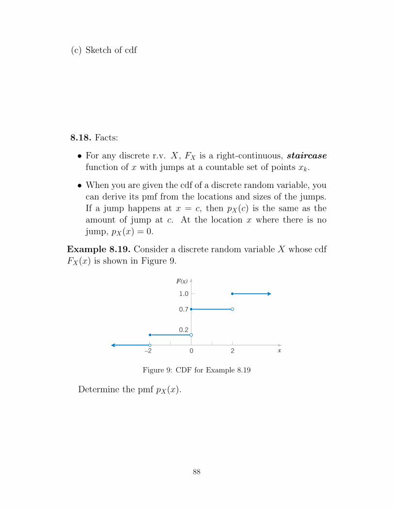
(c) Sketch of cdf
8.18. Facts:
• For any discrete r.v. X, FX is a right-continuous, staircasefunction of x with jumps at a countable set of points xk.
• When you are given the cdf of a discrete random variable, youcan derive its pmf from the locations and sizes of the jumps.If a jump happens at x = c, then pX(c) is the same as theamount of jump at c. At the location x where there is nojump, pX(x) = 0.
Example 8.19. Consider a discrete random variable X whose cdfFX(x) is shown in Figure 9. 3-3 CUMULATIVE DISTRIBUTION FUNCTIONS 73
0
0.2
2–2
0.7
1.0
x
F(x)
Figure 3-3 Cumulative distribution function forExample 3-7.
Figure 3-4 Cumulative distributionfunction for Example 3-8.
0 2
0.9971.000
x
0.886
1
F(x)
3-32. Determine the cumulative distribution function of therandom variable in Exercise 3-14.
3-33. Determine the cumulative distribution function forthe random variable in Exercise 3-15; also determine the fol-lowing probabilities:(a) (b)(c) (d)
3-34. Determine the cumulative distribution function for therandom variable in Exercise 3-16; also determine the followingprobabilities:(a) (b)(c) (d)
3-35. Determine the cumulative distribution function forthe random variable in Exercise 3-21.
3-36. Determine the cumulative distribution function forthe random variable in Exercise 3-22.
3-37. Determine the cumulative distribution function forthe random variable in Exercise 3-23.
3-38. Determine the cumulative distribution function forthe variable in Exercise 3-24.
Verify that the following functions are cumulative distributionfunctions, and determine the probability mass function and therequested probabilities.
3-39.
(a) (b)(c) (d)
3-40. Errors in an experimental transmission channel arefound when the transmission is checked by a certifier that de-tects missing pulses. The number of errors found in an eight-bit byte is a random variable with the following distribution:
F1x2 μ
0 x 10.7 1 x 40.9 4 x 71 7 x
P1X 22P11 X 22P1X 22P1X 32
F1x2 •0 x 10.5 1 x 31 3 x
P11 X 22P1X 22P1X 32P1X 1.52
P1X 02P11.1 X 12P1X 2.22P1X 1.252
Determine each of the following probabilities:(a) (b)(c) (d)(e)
3-41.
(a) (b)(c) (d)(e) (f)
3-42. The thickness of wood paneling (in inches) that a cus-tomer orders is a random variable with the following cumula-tive distribution function:
Determine the following probabilities:(a) (b)(c) (d)(e)
3-43. Determine the cumulative distribution function forthe random variable in Exercise 3-28.
3-44. Determine the cumulative distribution function forthe random variable in Exercise 3-29.
3-45. Determine the cumulative distribution function forthe random variable in Exercise 3-30.
3-46. Determine the cumulative distribution function forthe random variable in Exercise 3-31.
P1X 122P1X 142P1X 5162P1X 142P1X 1182
F1x2 μ
0 x 180.2 18 x 140.9 14 x 381 38 x
P110 X 102P10 X 102P1X 02P140 X 602P1X 402P1X 502
F1x2 μ
0 x 100.25 10 x 300.75 30 x 501 50 x
P1X 22P1X 42P1X 52P1X 72P1X 42
EXERCISES FOR SECTION 3-3
JWCL232_c03_066-106.qxd 1/7/10 10:58 AM Page 73
Figure 9: CDF for Example 8.19
Determine the pmf pX(x).
88
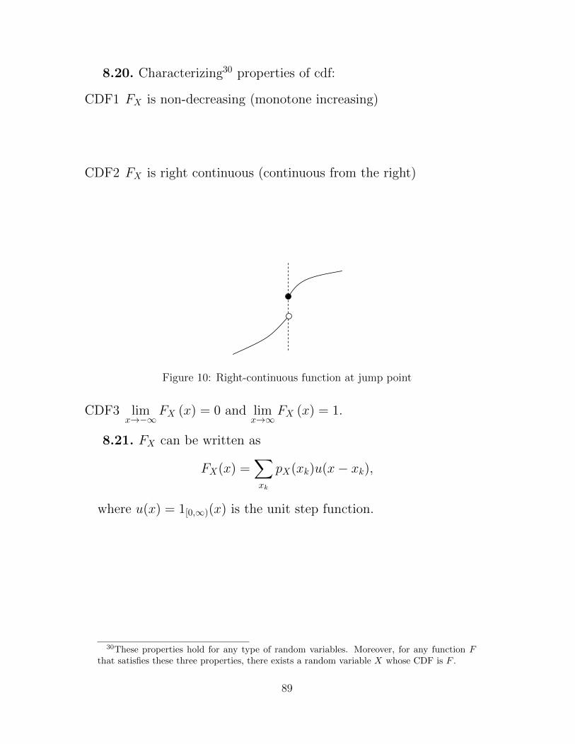
8.20. Characterizing30 properties of cdf:
CDF1 FX is non-decreasing (monotone increasing)
CDF2 FX is right continuous (continuous from the right)
x 0P X x
countable set C, 0XP C
XF is continuous
25) Every random variable can be written as a sum of a discrete random variable and a
continuous random variable.
26) A random variable can have at most countably many point x such that
0P X x .
27) The (cumulative) distribution function (cdf) induced by a probability P on
, is the function ,F x P x .
The (cumulative) distribution function (cdf) of the random variable X is the
function ,X
XF x P x P X x .
The distribution XP can be obtained from the distribution function by setting
,X
XP x F x ; that isXF uniquely determines
XP .
0 1XF
XF is non-decreasing
XF is right continuous:
x lim limX X X Xy x y xy x
F x F y F y F x P X x
.
lim 0Xx
F x
and lim 1Xx
F x
.
x lim lim ,X
X X Xy x y xy x
F x F y F y P x P X x
.
XP X x P x F x F x = the jump or saltus in F at x.
x y
,P x y F y F x
,P x y F y F x
Figure 10: Right-continuous function at jump point
CDF3 limx→−∞
FX (x) = 0 and limx→∞
FX (x) = 1.
8.21. FX can be written as
FX(x) =∑xk
pX(xk)u(x− xk),
where u(x) = 1[0,∞)(x) is the unit step function.
30These properties hold for any type of random variables. Moreover, for any function Fthat satisfies these three properties, there exists a random variable X whose CDF is F .
89
Sirindhorn International Institute of Technology
Thammasat University
School of Information, Computer and Communication Technology
ECS315 2013/1 Part III.2 Dr.Prapun
8.3 Families of Discrete Random Variables
Many physical systems can be modeled by the same or similarrandom experiments and random variables. In this subsection,we present the analysis of several discrete random variables thatfrequently arise in applications.31
Definition 8.22. X is uniformly distributed on a finite set Sif
pX(x) = P [X = x] =
1|S| , x ∈ S,0, otherwise,
• We write X ∼ U(S) or X ∼ Uniform(S).
• Read “X is uniform on S” or “X is a uniform random variableon set S”.
• The pmf is usually referred to as the uniform discrete distri-bution.
• Simulation: When the support S contains only consecutive in-tegers32, it can be generated by the command randi in MATLAB
(R2008b).
31As mention in 7.12, we often omit a discussion of the underlying sample space of therandom experiment and directly describe the distribution of a particular random variable.
32or, with minor manipulation, only uniformly spaced numbers
90

Example 8.23. X is uniformly distributed on 1, 2, . . . , n if
In MATLAB, X can be generated by randi(10).
Example 8.24. Uniform pmf is used when the random variablecan take finite number of “equally likely” or “totally random” val-ues.
• Classical game of chance / classical probability
• Fair gaming devices (well-balanced coins and dice, well-shuffleddecks of cards)
Example 8.25. Roll a fair dice. Let X be the outcome.
Definition 8.26. X is a Bernoulli random variable if
pX (x) =
1− p, x = 0,p, x = 1,0, otherwise,
p ∈ (0, 1)
• Write X ∼ B(1, p) or X ∼ Bernoulli(p)
• X takes only two values: 0 or 1
Definition 8.27. X is a binary random variable if
pX (x) =
1− p, x = a,p, x = b,0, otherwise,
p ∈ (0, 1), b > a.
• X takes only two values: a or b
91

Definition 8.28. X is a binomial random variable with sizen ∈ N and parameter p ∈ (0, 1) if
pX (x) =
(nx
)px(1− p)n−x, x ∈ 0, 1, 2, . . . , n,
0, otherwise(12)
• Write X ∼ B(n, p) or X ∼ binomial(p).
Observe that B(1, p) is Bernoulli with parameter p.
• To calculate pX(x), can use binopdf(x,n,p) in MATLAB.
• Interpretation: X is the number of successes in n independentBernoulli trials.
Example 8.29. An optical inspection system is to distinguishamong different part types. The probability of a correct classi-fication of any part is 0.98. Suppose that three parts are inspectedand that the classifications are independent.
(a) Let the random variable X denote the number of parts thatare correctly classified. Determine the probability mass func-tion of X. [15, Q3-20]
(b) Let the random variable Y denote the number of parts thatare incorrectly classified. Determine the probability massfunction of Y .
Solution :
(a) X is a binomial random variable with n = 3 and p = 0.98.Hence,
pX (x) =
(3x
)0.98x(0.02)3−x, x ∈ 0, 1, 2, 3,
0, otherwise(13)
In particular, pX(0) = 8 × 10⁻⁶, pX(1) = 0.001176, pX(2) =0.057624, and pX(3) = 0.941192. Note that in MATLAB, theseprobabilities can be calculated by evaluatingbinopdf(0:3,3,0.98).
92

(b) Y is a binomial random variable with n = 3 and p = 0.02.Hence,
pY (y) =
(3y
)0.02y(0.98)3−y, y ∈ 0, 1, 2, 3,
0, otherwise(14)
In particular, pY (0) = 0.941192, pY (1) = 0.057624, pY (2) =0.001176, and pY (3) = 8 × 10⁻⁶. Note that in MATLAB, theseprobabilities can be calculated by evaluatingbinopdf(0:3,3,0.02).
Alternatively, note that there are three parts. IfX of them areclassified correctly, then the number of incorrectly classifiedparts is n − X, which is what we defined as Y . Therefore,Y = 3 − X. Hence, pY (y) = P [Y = y] = P [3−X = y] =P [X = 3− y] = pX(3− y).
Example 8.30. Daily Airlines flies from Amsterdam to Londonevery day. The price of a ticket for this extremely popular flightroute is $75. The aircraft has a passenger capacity of 150. Theairline management has made it a policy to sell 160 tickets for thisflight in order to protect themselves against no-show passengers.Experience has shown that the probability of a passenger beinga no-show is equal to 0.1. The booked passengers act indepen-dently of each other. Given this overbooking strategy, what is theprobability that some passengers will have to be bumped from theflight?
Solution : This problem can be treated as 160 independenttrials of a Bernoulli experiment with a success rate of p = 9/10,where a passenger who shows up for the flight is counted as a suc-cess. Use the random variable X to denote number of passengersthat show up for a given flight. The random variable X is bino-mial distributed with the parameters n = 160 and p = 9/10. Theprobability in question is given by
P [X > 150] = 1− P [X ≤ 150] = 1− FX(150).
In MATLAB, we can enter 1-binocdf(150,160,9/10) to get 0.0359.Thus, the probability that some passengers will be bumped fromany given flight is roughly 3.6%. [21, Ex 4.1]
93
Definition 8.31. A geometric random variable X is defined bythe fact that for some constant β ∈ (0, 1),
pX(k + 1) = β × pX(k)
for all k ∈ S where S can be either N or N ∪ 0.(a) When its support is N = 1, 2, . . .,
pX(x) =
(1− β) βx−1, x = 1, 2, . . .0, otherwise.
• Write X ∼ G1 (β) or geometric1 (β).
• In MATLAB, to evaluate pX(x), use geopdf(x-1,1-β).
• Interpretation: X is the number of trials required inBernoulli trials to achieve the first success.
In particular, in a series of Bernoulli trials (independenttrials with constant probability p of a success), let therandom variable X denote the number of trials until thefirst success. Then X is a geometric random variable withparameter β = 1− p and
pX(x) =
(1− β) βx−1, x = 1, 2, . . .0, otherwise
=
p(1− p)x−1, x = 1, 2, . . .0, otherwise.
(b) When its support is N ∪ 0,
pX(x) =
(1− β) βx, x = 0, 1, 2, . . .0, otherwise
=
p(1− p)x, x = 0, 1, 2, . . .0, otherwise.
• Write X ∼ G0 (β) or geometric0 (β).
• In MATLAB, to evaluate pX(x), use geopdf(x,1-β).
• Interpretation: X is the number of failures in Bernoullitrials before the first success occurs.
94

8.32. In 1837, the famous French mathematician Poisson intro-duced a probability distribution that would later come to be knownas the Poisson distribution, and this would develop into one of themost important distributions in probability theory. As is often re-marked, Poisson did not recognize the huge practical importance ofthe distribution that would later be named after him. In his book,he dedicates just one page to this distribution. It was Bortkiewiczin 1898, who first discerned and explained the importance of thePoisson distribution in his book Das Gesetz der Kleinen Zahlen(The Law of Small Numbers). [21]
Definition 8.33. X is a Poisson random variable with param-eter α > 0 if
pX (x) =
e−αα
x
x! , x = 0, 1, 2, . . .0, otherwise
• In MATLAB, use poisspdf(x,alpha).
• Write X ∼ P (α) or Poisson(α).
• We will see later in Example 9.7 that α is the “average” orexpected value of X.
• Instead of X, Poisson random variable is usually denoted byΛ. The parameter α is often replaced by λτ where λ is referredto as the intensity/rate parameter of the distribution
Example 8.34. The first use of the Poisson model is said to havebeen by a Prussian (German) physician, Bortkiewicz, who foundthat the annual number of late-19th-century Prussian (German)soldiers kicked to death by horses fitted a Poisson distribution [6,p 150],[3, Ex 2.23]33.
33I. J. Good and others have argued that the Poisson distribution should be called theBortkiewicz distribution, but then it would be very difficult to say or write.
95

Example 8.35. The number of hits to a popular website duringa 1-minute interval is given by N ∼ P(α) where α = 2.
(a) Find the probability that there is at least one hit between3:00AM and 3:01AM.
(b) Find the probability that there are at least 2 hits during thetime interval above.
8.36. One of the reasons why Poisson distribution is important isbecause many natural phenomenons can be modeled by Poissonprocesses .
Definition 8.37. A Poisson process (PP) is a random arrange-ment of “marks” (denoted by “×” below) on the time line.
The “marks” may indicate the arrival times or occurrences ofevent/phenomenon of interest.
Example 8.38. Examples of processes that can be modeled byPoisson process include
(a) the sequence of times at which lightning strikes occur or mailcarriers get bitten within some region
(b) the emission of particles from a radioactive source
96
(c) the arrival of
• telephone calls at a switchboard or at an automatic phone-switching system
• urgent calls to an emergency center
• (filed) claims at an insurance company
• incoming spikes (action potential) to a neuron in humanbrain
(d) the occurrence of
• serious earthquakes
• traffic accidents
• power outages
in a certain area.
(e) page view requests to a website
8.39. It is convenient to consider the Poisson process in terms ofcustomers arriving at a facility.
We focus on a type of Poisson process that is called homogeneousPoisson process.
Definition 8.40. For homogeneous Poisson process, there isonly one parameter that describes the whole process. This numberis call the rate and usually denoted by λ.
Example 8.41. If you think about modeling customer arrival asa Poisson process with rate λ = 5 customers/hour, then it meansthat during any fixed time interval of duration 1 hour (say, fromnoon to 1PM), you expect to have about 5 customers arriving inthat interval. If you consider a time interval of duration two hours(say, from 1PM to 3PM), you expect to have about 2 × 5 = 10customers arriving in that time interval.
8.42. One important fact which we will revisit later is that, for ahomogeneous Poisson process, the number of arrivals during a timeinterval of duration T is a Poisson random variable with parameterα = λT .
97

Example 8.43. Examples of Poisson random variables :
• #photons emitted by a light source of intensity λ [photon-s/second] in time τ
• #atoms of radioactive material undergoing decay in time τ
• #clicks in a Geiger counter in τ seconds when the averagenumber of click in 1 second is λ.
• #dopant atoms deposited to make a small device such as anFET
• #customers arriving in a queue or workstations requestingservice from a file server in time τ
• Counts of demands for telephone connections in time τ
• Counts of defects in a semiconductor chip.
Example 8.44. Thongchai produces a new hit song every 7 monthson average. Assume that songs are produced according to a Pois-son process. Find the probability that Thongchai produces morethan two hit songs in 1 year.
8.45. Poisson approximation of Binomial distribution: Whenp is small and n is large, B(n, p) can be approximated by P(np)
(a) In a large number of independent repetitions of a Bernoullitrial having a small probability of success, the total number ofsuccesses is approximately Poisson distributed with parame-ter α = np, where n = the number of trials and p = theprobability of success. [21, p 109]
98

(b) More specifically, suppose Xn ∼ B(n, pn). If pn → 0 andnpn → α as n→∞, then
P [Xn = k] =
(n
k
)pkn(1− pn)n−k → e−α
αk
k!.
Example 8.46. Consider Xn ∼ B(n, 1/n).
Example 8.47. Recall that Bortkiewicz applied the Poisson modelto the number of Prussian cavalry deaths attributed to fatal horsekicks. Here, indeed, one encounters a very large number of trials(the Prussian cavalrymen), each with a very small probability of“success” (fatal horse kick).
8.48. Summary:
X ∼ Support SX pX (x)
Uniform Un 1, 2, . . . , n 1n
U0,1,...,n−1 0, 1, . . . , n− 1 1n
Bernoulli B(1, p) 0, 1
1− p, x = 0p, x = 1
Binomial B(n, p) 0, 1, . . . , n(nx
)px(1− p)n−x
Geometric G0(β) N ∪ 0 (1− β)βx
Geometric G1(β) N (1− β)βx−1
Poisson P(α) N ∪ 0 e−α αx
x!
Table 3: Examples of probability mass functions. Here, p, β ∈ (0, 1). α > 0.n ∈ N
99

8.4 Some Remarks
8.49. Sometimes, it is useful to define and think of pmf as a vectorp of probabilities.
When you use MATLAB, it is also useful to keep track of thevalues of x corresponding to the probabilities in p. This can bedone via defining a vector x.
Example 8.50. For B(3, 1
3
), we may define
x = [0, 1, 2, 3]
and
p =
[(3
0
)(1
3
)0(2
3
)3
,
(3
1
)(1
3
)1(2
3
)2
,
(3
2
)(1
3
)2(2
3
)1
,
(3
3
)(1
3
)3(2
3
)0]
=
[8
27,4
9,2
9,
1
27
]8.51. At this point, we have a couple of ways to define probabil-
ities that are associated with a random variable X
(a) We can define P [X ∈ B] for all possible set B.
(b) For discrete random variable, we only need to define its pmfpX(x) which is defined as P [X = x] = P [X ∈ x].
(c) We can also define the cdf FX(x).
Definition 8.52. If pX(c) = 1, that is P [X = c] = 1, for someconstant c, then X is called a degenerated random variable.
100
9 Expectation and Variance
Two numbers are often used to summarize a probability distribu-tion for a random variable X. The mean is a measure of the cen-ter or middle of the probability distribution, and the variance is ameasure of the dispersion, or variability in the distribution. Thesetwo measures do not uniquely identify a probability distribution.That is, two different distributions can have the same mean andvariance. Still, these measures are simple, useful summaries of theprobability distribution of X.
9.1 Expectation of Discrete Random Variable
The most important characteristic of a random variable is its ex-pectation. Synonyms for expectation are expected value, mean,and first moment.
The definition of expectation is motivated by the conventionalidea of numerical average. Recall that the numerical average of nnumbers, say a1, a2, . . . , an is
1
n
n∑k=1
ak.
We use the average to summarize or characterize the entire collec-tion of numbers a1, . . . , an with a single value.
Example 9.1. Consider 10 numbers: 5, 2, 3, 2, 5, -2, 3, 2, 5, 2.The average is
5 + 2 + 3 + 2 + 5 + (−2) + 3 + 2 + 5 + 2
10=
27
10= 2.7.
We can rewrite the above calculation as
−2× 1
10+ 2× 4
10+ 3× 2
10+ 5× 3
10
101

Definition 9.2. Suppose X is a discrete random variable, we de-fine the expectation (or mean or expected value) of X by
EX =∑x
x× P [X = x] =∑x
x× pX(x). (15)
In other words, The expected value of a discrete random variableis a weighted mean of the values the random variable can take onwhere the weights come from the pmf of the random variable.
• Some references use mX or µX to represent EX.
• For conciseness, we simply write x under the summation sym-bol in (15); this means that the sum runs over all x values inthe support of X. (Of course, for x outside of the support,pX(x) is 0 anyway.)
9.3. Analogy: In mechanics, think of point masses on a line witha mass of pX(x) kg. at a distance x meters from the origin.
In this model, EX is the center of mass (the balance point).This is why pX(x) is called probability mass function.
Example 9.4. When X ∼ Bernoulli(p) with p ∈ (0, 1),
Note that, since X takes only the values 0 and 1, its expectedvalue p is “never seen”.
9.5. Interpretation: The expected value is in general not a typicalvalue that the random variable can take on. It is often helpful tointerpret the expected value of a random variable as the long-runaverage value of the variable over many independent repetitionsof an experiment
Example 9.6. pX (x) =
1/4, x = 03/4, x = 20, otherwise
102

Example 9.7. For X ∼ P(α),
EX =∞∑i=0
ie−α(α)i
i!=
∞∑i=1
e−α(α)i
i!i+ 0 = e−α (α)
∞∑i=1
(α)i−1
(i− 1)!
= e−αα∞∑k=0
αk
k!= e−ααeα = α.
Example 9.8. For X ∼ B(n, p),
EX =
n∑i=0
i
(n
i
)pi(1− p)n−i =
n∑i=1
in!
i! (n− i)!pi(1− p)n−i
= n
n∑i=1
(n− 1)!
(i− 1)! (n− i)!pi(1− p)n−i = n
n∑i=1
(n− 1
i− 1
)pi(1− p)n−i
Let k = i− 1. Then,
EX = n
n−1∑k=0
(n− 1
k
)pk+1(1− p)n−(k+1) = np
n−1∑k=0
(n− 1
k
)pk(1− p)n−1−k
We now have the expression in the form that we can apply thebinomial theorem which finally gives
EX = np(p+ (1− p))n−1 = np.
We shall revisit this example again using another approach in Ex-ample 11.48.
Example 9.9. Pascal’s wager : Suppose you concede that youdon’t know whether or not God exists and therefore assign a 50percent chance to either proposition. How should you weigh theseodds when deciding whether to lead a pious life? If you act piouslyand God exists, Pascal argued, your gain–eternal happiness–is in-finite. If, on the other hand, God does not exist, your loss, ornegative return, is small–the sacrifices of piety. To weigh thesepossible gains and losses, Pascal proposed, you multiply the prob-ability of each possible outcome by its payoff and add them all up,forming a kind of average or expected payoff. In other words, themathematical expectation of your return on piety is one-half infin-ity (your gain if God exists) minus one-half a small number (yourloss if he does not exist). Pascal knew enough about infinity to
103
know that the answer to this calculation is infinite, and thus theexpected return on piety is infinitely positive. Every reasonableperson, Pascal concluded, should therefore follow the laws of God.[14, p 76]
• Pascals wager is often considered the founding of the math-ematical discipline of game theory, the quantitative study ofoptimal decision strategies in games.
9.10. Technical issue: Definition (15) is only meaningful if thesum is well defined.
The sum of infinitely many nonnegative terms is always well-defined, with +∞ as a possible value for the sum.
• Infinite Expectation : Consider a random variable X whosepmf is defined by
pX (x) =
1cx2 , x = 1, 2, 3, . . .0, otherwise
Then, c =∑∞
n=11n2 which is a finite positive number (π2/6).
However,
EX =∞∑k=1
kpX(k) =∞∑k=1
k1
c
1
k2=
1
c
∞∑k=1
1
k= +∞.
Some care is necessary when computing expectations of signedrandom variables that take infinitely many values.
• The sum over countably infinite many terms is not always welldefined when both positive and negative terms are involved.
• For example, the infinite series 1−1 + 1−1 + . . . has the sum0 when you sum the terms according to (1−1)+(1−1)+ · · · ,whereas you get the sum 1 when you sum the terms accordingto 1 + (−1 + 1) + (−1 + 1) + (−1 + 1) + · · · .
• Such abnormalities cannot happen when all terms in the infi-nite summation are nonnegative.
104

It is the convention in probability theory that EX should be eval-uated as
EX =∑x≥0
xpX(x)−∑x<0
(−x)pX(x),
• If at least one of these sums is finite, then it is clear whatvalue should be assigned as EX.
• If both sums are +∞, then no value is assigned to EX, andwe say that EX is undefined.
Example 9.11. Undefined Expectation: Let
pX (x) =
1
2cx2 , x = ±1,±2,±3, . . .0, otherwise
Then,
EX =∞∑k=1
kpX (k)−−1∑
k=−∞(−k) pX (k).
The first sum gives
∞∑k=1
kpX (k) =∞∑k=1
k1
2ck2=
1
2c
∞∑k=1
1
k=∞2c.
The second sum gives
−1∑k=−∞
(−k) pX (k) =∞∑k=1
kpX (−k) =∞∑k=1
k1
2ck2=
1
2c
∞∑k=1
1
k=∞2c.
Because both sums are infinite, we conclude that EX is undefined.
9.12. More rigorously, to define EX, we let X+ = max X, 0 andX− = −min X, 0. Then observe that X = X+ − X− and thatboth X+ and X− are nonnegative r.v.’s. We say that a randomvariable X admits an expectation if EX+ and EX− are notboth equal to +∞. In which case, EX = EX+ − EX−.
105
9.2 Function of a Discrete Random Variable
Given a random variable X, we will often have occasion to definea new random variable by Y ≡ g(X), where g(x) is a real-valuedfunction of the real-valued variable x. More precisely, recall thata random variable X is actually a function taking points of thesample space, ω ∈ Ω, into real numbers X(ω). Hence, we have thefollowing definition
Definition 9.13. The notation Y = g(X) is actually shorthandfor Y (ω) := g(X(ω)).
• The random variable Y = g(X) is sometimes called derivedrandom variable.
Example 9.14. Let
pX (x) =
1cx
2, x = ±1,±20, otherwise
andY = X4.
Find pY (y) and then calculate EY .
9.15. For discrete random variable X, the pmf of a derived ran-dom variable Y = g(X) is given by
pY (y) =∑
x:g(x)=y
pX(x).
106

Note that the sum is over all x in the support of X which satisfyg(x) = y.
Example 9.16. A “binary” random variable X takes only twovalues a and b with
P [X = b] = 1− P [X = a] = p.
X can be expressed as X = (b − a)I + a, where I is a Bernoullirandom variable with parameter p.
9.3 Expectation of a Function of a Discrete RandomVariable
Recall that for discrete random variable X, the pmf of a derivedrandom variable Y = g(X) is given by
pY (y) =∑
x:g(x)=y
pX(x).
If we want to compute EY , it might seem that we first have tofind the pmf of Y . Typically, this requires a detailed analysis of gwhich can be complicated, and it is avoided by the following result.
9.17. Suppose X is a discrete random variable.
E [g(X)] =∑x
g(x)pX(x).
This is referred to as the law/rule of the lazy/unconciousstatistician (LOTUS) [22, Thm 3.6 p 48],[9, p. 149],[8, p. 50]because it is so much easier to use the above formula than to firstfind the pmf of Y . It is also called substitution rule [21, p 271].
Example 9.18. Back to Example 9.14. Recall that
pX (x) =
1cx
2, x = ±1,±20, otherwise
(a) When Y = X4, EY =
107

(b) E [2X − 1]
9.19. Caution: A frequently made mistake of beginning studentsis to set E [g(X)] equal to g (EX). In general, E [g(X)] 6= g (EX).
(a) In particular, E[
1X
]is not the same as 1
EX .
(b) An exception is the case of a linear function g(x) = ax + b.See also (9.23).
Example 9.20. Continue from Example 9.4. ForX ∼ Bernoulli(p),
(a) EX = p
(b) E[X2]
= 02 × (1− p) + 12 × p = p 6= (EX)2.
Example 9.21. Continue from Example 9.7. Suppose X ∼ P(α).
E[X2]
=∞∑i=0
i2e−ααi
i!= e−αα
∞∑i=1
iαi−1
(i− 1)!(16)
We can evaluate the infinite sum in (16) by rewriting i as i−1+1:∞∑i=1
iαi−1
(i− 1)!=
∞∑i=1
(i− 1 + 1)αi−1
(i− 1)!=
∞∑i=1
(i− 1)αi−1
(i− 1)!+
∞∑i=1
αi−1
(i− 1)!
= α∞∑i=2
αi−2
(i− 2)!+∞∑i=1
αi−1
(i− 1)!= αeα + eα = eα(α+ 1).
Plugging this back into (16), we get
E[X2]
= α (α + 1) = α2 + α.
9.22. Continue from Example 9.8. For X ∼ B(n, p), one can findE[X2]
= np(1− p) + (np)2.
108

9.23. Some Basic Properties of Expectations
(a) For c ∈ R, E [c] = c
(b) For c ∈ R, E [X + c] = EX + c and E [cX] = cEX
(c) For constants a, b, we have
E [aX + b] = aEX + b.
(d) For constants c1 and c2,
E [c1g1(X) + c2g2(X)] = c1E [g1(X)] + c2E [g2(X)] .
(e) For constants c1, c2, . . . , cn,
E
[n∑k=1
ckgk(X)
]=
n∑k=1
ckE [gk(X)] .
Definition 9.24. Some definitions involving expectation of a func-tion of a random variable:
(a) Absolute moment : E[|X|k
], where we define E
[|X|0
]= 1
(b) Moment : mk = E[Xk]
= the kth moment of X, k ∈ N.
• The first moment of X is its expectation EX.
• The second moment of X is E[X2].
109
9.4 Variance and Standard Deviation
An average (expectation) can be regarded as one number thatsummarizes an entire probability model. After finding an average,someone who wants to look further into the probability modelmight ask, “How typical is the average?” or, “What are thechances of observing an event far from the average?” A measureof dispersion/deviation/spread is an answer to these questionswrapped up in a single number. (The opposite of this measure isthe peakedness.) If this measure is small, observations are likelyto be near the average. A high measure of dispersion suggests thatit is not unusual to observe events that are far from the average.
Example 9.25. Consider your score on the midterm exam. Afteryou find out your score is 7 points above average, you are likely toask, “How good is that? Is it near the top of the class or somewherenear the middle?”.
Example 9.26. In the case that the random variable X is therandom payoff in a game that can be repeated many times underidentical conditions, the expected value of X is an informativemeasure on the grounds of the law of large numbers. However, theinformation provided by EX is usually not sufficient when X isthe random payoff in a nonrepeatable game.
Suppose your investment has yielded a profit of $3,000 and youmust choose between the following two options:
• the first option is to take the sure profit of $3,000 and
• the second option is to reinvest the profit of $3,000 under thescenario that this profit increases to $4,000 with probability0.8 and is lost with probability 0.2.
The expected profit of the second option is
0.8× $4, 000 + 0.2× $0 = $3, 200
and is larger than the $3,000 from the first option. Nevertheless,most people would prefer the first option. The downside risk istoo big for them. A measure that takes into account the aspect ofrisk is the variance of a random variable. [21, p 35]
110

9.27. The most important measures of dispersion are thestandard deviation and its close relative, the variance.
Definition 9.28. Variance :
VarX = E[(X − EX)2
]. (17)
• Read “the variance of X”
• Notation: DX , or σ2 (X), or σ2X , or VX [22, p. 51]
• In some references, to avoid confusion from the two expecta-tion symbols, they first define m = EX and then define thevariance of X by
VarX = E[(X −m)2
].
• We can also calculate the variance via another identity:
VarX = E[X2]− (EX)2
• The units of the variance are squares of the units of the ran-dom variable.
9.29. Basic properties of variance:
• VarX ≥ 0.
• VarX ≤ E[X2].
• Var[cX] = c2 VarX.
• Var[X + c] = VarX.
• Var[aX + b] = a2 VarX.
111

Definition 9.30. Standard Deviation :
σX =√
Var[X].
• It is useful to work with the standard deviation since it hasthe same units as EX.
• Informally we think of outcomes within ±σX of EX as beingin the center of the distribution. Some references would in-formally interpret sample values within ±σX of the expectedvalue, x ∈ [EX − σX ,EX + σX ], as “typical” values of X andother values as “unusual”.
• σaX+b = |a|σX .
9.31. σX and√
VarX: Note that the√· function is a strictly
increasing function. Because σX =√
VarX, if one of them islarge, another one is also large. Therefore, both values quantifythe amount of spread/dispersion in RV X (which can be observedfrom the spread or dispersion of the pmf or the histogram or therelative frequency graph). However, VarX does not have the sameunit as the RV X.
9.32. In finance, standard deviation is a key concept and is usedto measure the volatility (risk) of investment returns and stockreturns.
It is common wisdom in finance that diversification of a portfolioof stocks generally reduces the total risk exposure of the invest-ment. We shall return to this point in Example 11.68.
Example 9.33. Continue from Example 9.25. If the standarddeviation of exam scores is 12 points, the student with a score of+7 with respect to the mean can think of herself in the middle ofthe class. If the standard deviation is 3 points, she is likely to benear the top.
Example 9.34. Suppose X ∼ Bernoulli(p).
(a) E[X2]
= 02 × (1− p) + 12 × p = p.
112
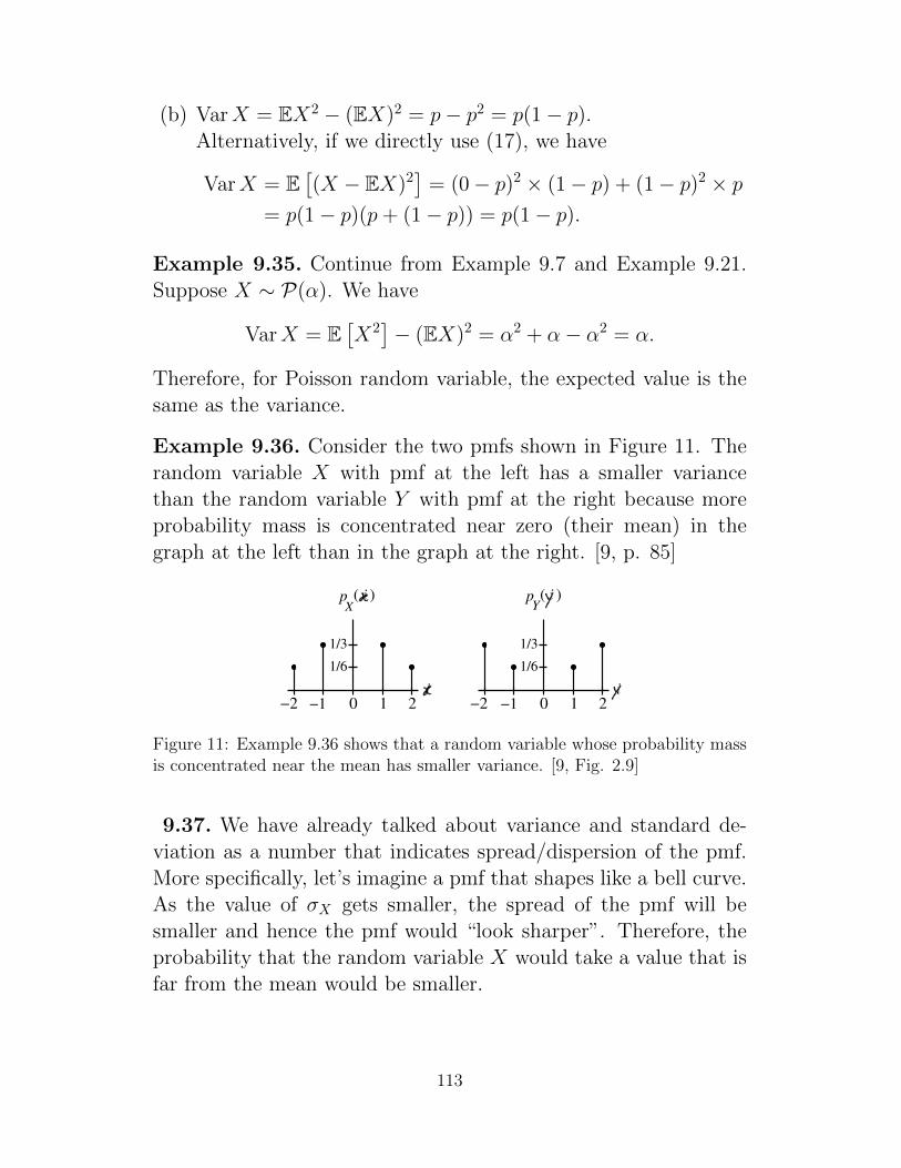
(b) VarX = EX2 − (EX)2 = p− p2 = p(1− p).Alternatively, if we directly use (17), we have
VarX = E[(X − EX)2
]= (0− p)2 × (1− p) + (1− p)2 × p
= p(1− p)(p+ (1− p)) = p(1− p).
Example 9.35. Continue from Example 9.7 and Example 9.21.Suppose X ∼ P(α). We have
VarX = E[X2]− (EX)2 = α2 + α− α2 = α.
Therefore, for Poisson random variable, the expected value is thesame as the variance.
Example 9.36. Consider the two pmfs shown in Figure 11. Therandom variable X with pmf at the left has a smaller variancethan the random variable Y with pmf at the right because moreprobability mass is concentrated near zero (their mean) in thegraph at the left than in the graph at the right. [9, p. 85]
2.4 Expectation 85
The variance is the average squared deviation of X about its mean. The variance character-
izes how likely it is to observe values of the random variable far from its mean. For example,
consider the two pmfs shown in Figure 2.9. More probability mass is concentrated near zero
in the graph at the left than in the graph at the right.
ipX
( )
0 1 2−1i
−2
1/6
1/3
Yip ( )
0 1 2−1i
−2
1/6
1/3
Figure 2.9. Example 2.27 shows that the random variable X with pmf at the left has a smaller variance than the
random variable Y with pmf at the right.
Example 2.27. Let X and Y be the random variables with respective pmfs shown in
Figure 2.9. Compute var(X) and var(Y ).
Solution. By symmetry, both X and Y have zero mean, and so var(X) = E[X2] and
var(Y ) = E[Y 2]. Write
E[X2] = (−2)2 16+(−1)2 1
3+(1)2 1
3+(2)2 1
6= 2,
and
E[Y 2] = (−2)2 13+(−1)2 1
6+(1)2 1
6+(2)2 1
3= 3.
Thus, X and Y are both zero-mean random variables taking the values ±1 and ±2. But Y
is more likely to take values far from its mean. This is reflected by the fact that var(Y ) >var(X).
When a random variable does not have zero mean, it is often convenient to use the
variance formula,
var(X) = E[X2]− (E[X ])2, (2.17)
which says that the variance is equal to the second moment minus the square of the first
moment. To derive the variance formula, write
var(X) := E[(X −m)2]
= E[X2 −2mX +m2]
= E[X2]−2mE[X ]+m2, by linearity,
= E[X2]−m2
= E[X2]− (E[X ])2.
The standard deviation of X is defined to be the positive square root of the variance. Since
the variance of a random variable is often denoted by the symbol σ2, the standard deviation
is denoted by σ .
Figure 11: Example 9.36 shows that a random variable whose probability massis concentrated near the mean has smaller variance. [9, Fig. 2.9]
9.37. We have already talked about variance and standard de-viation as a number that indicates spread/dispersion of the pmf.More specifically, let’s imagine a pmf that shapes like a bell curve.As the value of σX gets smaller, the spread of the pmf will besmaller and hence the pmf would “look sharper”. Therefore, theprobability that the random variable X would take a value that isfar from the mean would be smaller.
113

The next property involves the use of σX to bound “the tailprobability” of a random variable.
9.38. Chebyshev’s Inequality :
P [|X − EX| ≥ α] ≤ σ2X
α2
or equivalently
P [|X − EX| ≥ nσX ] ≤ 1
n2
• Useful only when α > σX
Example 9.39. If X has mean m and variance σ2, it is sometimesconvenient to introduce the normalized random variable
Y =X −mσ
.
Definition 9.40. Central Moments : A generalization of thevariance is the nth central moment which is defined to be
µn = E [(X − EX)n] .
(a) µ1 = E [X − EX] = 0.
(b) µ2 = σ2X = VarX: the second central moment is the variance.
114

Sirindhorn International Institute of Technology
Thammasat University
School of Information, Computer and Communication Technology
ECS315 2013/1 Part IV.1 Dr.Prapun
10 Continuous Random Variables
10.1 From Discrete to Continuous Random Variables
In many practical applications of probability, physical situationsare better described by random variables that can take on a con-tinuum of possible values rather than a discrete number of values.For this type of random variable, the interesting fact is that
• any individual value has probability zero:
P [X = x] = 0 for all x (18)
and that
• the support is always uncountable.
These random variables are called continuous random vari-ables.
10.1. We can see from (18) that the pmf is going to be useless forthis type of random variable. It turns out that the cdf FX is stilluseful and we shall introduce another useful function called prob-ability density function (pdf) to replace the role of pmf. However,integral calculus34 is required to formulate this continuous analogof a pmf.
10.2. In some cases, the random variable X is actually discretebut, because the range of possible values is so large, it might bemore convenient to analyze X as a continuous random variable.
34This is always a difficult concept for the beginning student.
115

Example 10.3. Suppose that current measurements are read froma digital instrument that displays the current to the nearest one-hundredth of a mA. Because the possible measurements are lim-ited, the random variable is discrete. However, it might be a moreconvenient, simple approximation to assume that the current mea-surements are values of a continuous random variable.
Example 10.4. If you can measure the heights of people withinfinite precision, the height of a randomly chosen person is a con-tinuous random variable. In reality, heights cannot be measuredwith infinite precision, but the mathematical analysis of the dis-tribution of heights of people is greatly simplified when using amathematical model in which the height of a randomly chosenperson is modeled as a continuous random variable. [21, p 284]
Example 10.5. Continuous random variables are important mod-els for
(a) voltages in communication receivers
(b) file download times on the Internet
(c) velocity and position of an airliner on radar
(d) lifetime of a battery
(e) decay time of a radioactive particle
(f) time until the occurrence of the next earthquake in a certainregion
Example 10.6. The simplest example of a continuous randomvariable is the “random choice” of a number from the interval(0, 1).
• In MATLAB, this can be generated by the command rand.In Excel, use rand().
• The generation is “unbiased” in the sense that “any numberin the range is as likely to occur as another number.”
• Histogram is flat over (0, 1).
• Formally, this is called a uniform RV on the interval (0, 1).
116

Definition 10.7. We say that X is a continuous random vari-able35 if we can find a (real-valued) function36 f such that, for anyset B, P [X ∈ B] has the form
P [X ∈ B] =
∫B
f(x)dx. (19)
• In particular,
P [a ≤ X ≤ b] =
∫ b
a
f(x)dx. (20)
In other words, the area under the graph of f(x) betweenthe points a and b gives the probability P [a ≤ X ≤ b].
• The function f is called the probability density function(pdf) or simply density.
• When we want to emphasize that the function f is a densityof a particular random variable X, we write fX instead of f .
35To be more rigorous, this is the definition for absolutely continuous random variable. Atthis level, we will not distinguish between the continuous random variable and absolutelycontinuous random variable. When the distinction between them is considered, a randomvariable X is said to be continuous (not necessarily absolutely continuous) when condition (18)is satisfied. Alternatively, condition (18) is equivalent to requiring the cdf FX to be continuous.Another fact worth mentioning is that if a random variable is absolutely continuous, then itis continuous. So, absolute continuity is a stronger condition.
36Strictly speaking, δ-“function” is not a function; so, can’t use δ-function here.
117

206 Part 2: Probability
learningobjectives
After reading thischapter, you should
be able to:
• Understand the nature and the applications of the normal distribution.
• Use the standard normal distribution and z-scores to determine probabilitiesassociated with the normal distribution.
• Use the normal distribution to approximate the binomial distribution.
• Understand the nature and the applications of the exponential distribution,including its relationship to the Poisson distribution of Chapter 6.
• Use the computer in determining probabilities associated with the normal andexponential distributions.
7.1 INTRODUCTION
Chapter 6 dealt with probability distributions for discrete random variables,which can take on only certain values along an interval, with the possible valueshaving gaps between them. This chapter presents several continuous probabilitydistributions; these describe probabilities associated with random variables thatare able to assume any of an infinite number of values along an interval.
Discrete probability distributions can be expressed as histograms, where theprobabilities for the various x values are expressed by the heights of a series ofvertical bars. In contrast, continuous probability distributions are smooth curves,where probabilities are expressed as areas under the curves. The curve is a func-tion of x, and f(x) is referred to as a probability density function. Since the con-tinuous random variable x can be in an infinitely small interval along a range orcontinuum, the probability that x will take on any exact value may be regarded aszero. Therefore, we can speak of probabilities only in terms of the probability thatx will be within a specified interval of values. For a continuous random variable,the probability distribution will have the following characteristics:
The probability distribution for a continuous random variable:
1. The vertical coordinate is a function of x, described as f(x) and referred to asthe probability density function.
2. The range of possible x values is along the horizontal axis.3. The probability that x will take on a value between a and b will be the
area under the curve between points a and b, as shown in Figure 7.1. The
a bx
f(x)
Area = P(a ≤ x ≤ b)
FIGURE 7.1For a continuous randomvariable, the probability dis-tribution is described by acurve called the probabilitydensity function, f(x). Thetotal area beneath the curveis 1.0, and the probabilitythat x will take on somevalue between a and b isthe area beneath the curvebetween points a and b.
Figure 12: For a continuous random variable, the probability distribution isdescribed by a curve called the probability density function, f(x). The totalarea beneath the curve is 1.0, and the probability that X will take on somevalue between a and b is the area beneath the curve between points a and b.
Example 10.8. For the random variable generated by the rand
command in MATLAB37 or the rand() command in Excel,
Definition 10.9. Recall that the support SX of a random variableX is any set S such that P [X ∈ S] = 1. For continuous randomvariable, SX is usually set to be x : fX(x) > 0.
37The rand command in MATLAB is an approximation for two reasons:
(a) It produces pseudorandom numbers; the numbers seem random but are actually theoutput of a deterministic algorithm.
(b) It produces a double precision floating point number, represented in the computerby 64 bits. Thus MATLAB distinguishes no more than 264 unique double precisionfloating point numbers. By comparison, there are uncountably infinite real numbers inthe interval from 0 to 1.
118

10.2 Properties of PDF and CDF for Continuous Ran-dom Variables
10.10. fX is determined only almost everywhere38. That is, givena pdf f for a random variable X, if we construct a function g bychanging the function f at a countable number of points39, then gcan also serve as a pdf for X.
10.11. The cdf of any kind of random variable X is defined as
FX(x) = P [X ≤ x] .
Note that even through there are more than one valid pdfs forany given random variable, the cdf is unique. There is only onecdf for each random variable.
10.12. For continuous random variable, given the pdf fX(x), wecan find the cdf of X by
FX(x) = P [X ≤ x] =
∫ x
−∞fX(t)dt.
10.13. Given the cdf FX(x), we can find the pdf fX(x) by
• If FX is differentiable at x, we will set
d
dxFX(x) = fX(x).
• If FX is not differentiable at x, we can set the values of fX(x)to be any value. Usually, the values are selected to give simpleexpression. (In many cases, they are simply set to 0.)
38Lebesgue-a.e, to be exact39More specifically, if g = f Lebesgue-a.e., then g is also a pdf for X.
119
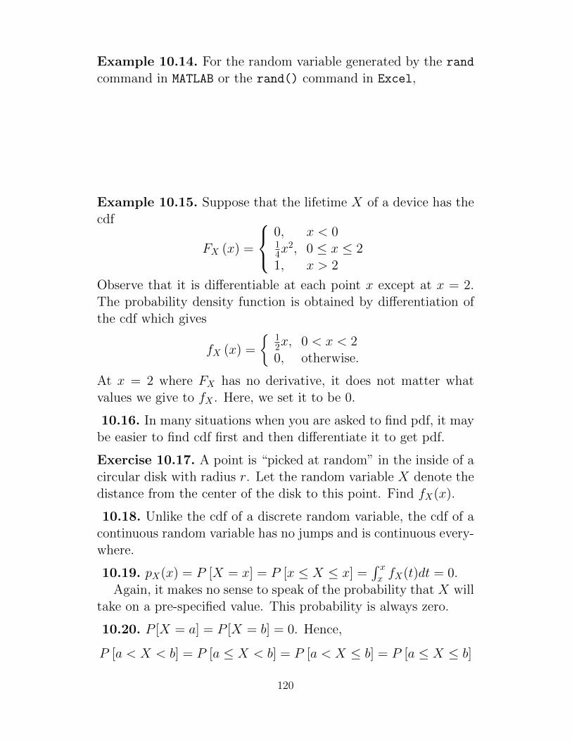
Example 10.14. For the random variable generated by the rand
command in MATLAB or the rand() command in Excel,
Example 10.15. Suppose that the lifetime X of a device has thecdf
FX (x) =
0, x < 014x
2, 0 ≤ x ≤ 21, x > 2
Observe that it is differentiable at each point x except at x = 2.The probability density function is obtained by differentiation ofthe cdf which gives
fX (x) =
12x, 0 < x < 20, otherwise.
At x = 2 where FX has no derivative, it does not matter whatvalues we give to fX . Here, we set it to be 0.
10.16. In many situations when you are asked to find pdf, it maybe easier to find cdf first and then differentiate it to get pdf.
Exercise 10.17. A point is “picked at random” in the inside of acircular disk with radius r. Let the random variable X denote thedistance from the center of the disk to this point. Find fX(x).
10.18. Unlike the cdf of a discrete random variable, the cdf of acontinuous random variable has no jumps and is continuous every-where.
10.19. pX(x) = P [X = x] = P [x ≤ X ≤ x] =∫ xx fX(t)dt = 0.
Again, it makes no sense to speak of the probability that X willtake on a pre-specified value. This probability is always zero.
10.20. P [X = a] = P [X = b] = 0. Hence,
P [a < X < b] = P [a ≤ X < b] = P [a < X ≤ b] = P [a ≤ X ≤ b]
120

• The corresponding integrals over an interval are not affectedby whether or not the endpoints are included or excluded.
• When we work with continuous random variables, it is usuallynot necessary to be precise about specifying whether or nota range of numbers includes the endpoints. This is quite dif-ferent from the situation we encounter with discrete randomvariables where it is critical to carefully examine the type ofinequality.
10.21. fX is nonnegative and∫R fX(x)dx = 1.
Example 10.22. Random variable X has pdf
fX(x) =
ce−2x, x > 00, otherwise
Find the constant c and sketch the pdf.
Definition 10.23. A continuous random variable is called expo-nential if its pdf is given by
fX (x) =
λe−λx, x > 0,0, x ≤ 0
for some λ > 0
Theorem 10.24. Any nonnegative40 function that integrates toone is a probability density function (pdf) of some randomvariable [9, p.139].
40or nonnegative a.e.
121
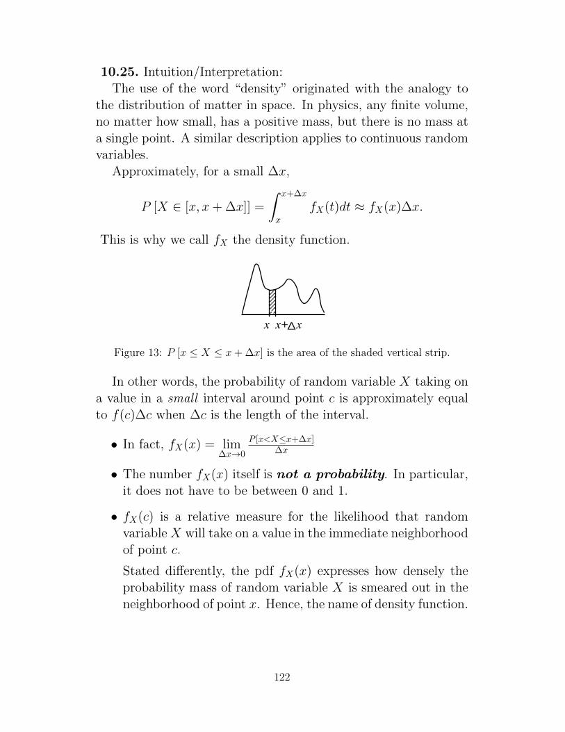
10.25. Intuition/Interpretation:The use of the word “density” originated with the analogy to
the distribution of matter in space. In physics, any finite volume,no matter how small, has a positive mass, but there is no mass ata single point. A similar description applies to continuous randomvariables.
Approximately, for a small ∆x,
P [X ∈ [x, x+ ∆x]] =
∫ x+∆x
x
fX(t)dt ≈ fX(x)∆x.
This is why we call fX the density function.
4.1 Densities and probabilities 139
Definition
We say that X is a continuous random variable if P(X ∈ B) has the form
P(X ∈ B) =∫
Bf (t)dt :=
∫ ∞
−∞IB(t) f (t)dt (4.1)
for some integrable function f .a Since P(X ∈ IR) = 1, the function f must integrate to one;
i.e.,∫ ∞−∞ f (t)dt = 1. Further, since P(X ∈ B) ≥ 0 for all B, it can be shown that f must be
nonnegative.1 A nonnegative function that integrates to one is called a probability density
function (pdf).
Usually, the set B is an interval such as B = [a,b]. In this case,
P(a ≤ X ≤ b) =∫ b
af (t)dt.
See Figure 4.1(a). Computing such probabilities is analogous to determining the mass of a
piece of wire stretching from a to b by integrating its mass density per unit length from a to
b. Since most probability densities we work with are continuous, for a small interval, say
[x,x+∆x], we have
P(x ≤ X ≤ x+∆x) =∫ x+∆x
xf (t)dt ≈ f (x)∆x.
See Figure 4.1(b).
(a) (b)
a b x+x x
Figure 4.1. (a) P(a ≤ X ≤ b) =∫ b
a f (t)dt is the area of the shaded region under the density f (t). (b) P(x ≤ X ≤x+∆x) =
∫ x+∆xx f (t)dt is the area of the shaded vertical strip.
Note that for random variables with a density,
P(a ≤ X ≤ b) = P(a < X ≤ b) = P(a ≤ X < b) = P(a < X < b)
since the corresponding integrals over an interval are not affected by whether or not the
endpoints are included or excluded.
Some common densities
Here are some examples of continuous random variables. A summary of the more com-
mon ones can be found on the inside of the back cover.
aLater, when more than one random variable is involved, we write fX (x) instead of f (x).
Figure 13: P [x ≤ X ≤ x+ ∆x] is the area of the shaded vertical strip.
In other words, the probability of random variable X taking ona value in a small interval around point c is approximately equalto f(c)∆c when ∆c is the length of the interval.
• In fact, fX(x) = lim∆x→0
P [x<X≤x+∆x]∆x
• The number fX(x) itself is not a probability. In particular,it does not have to be between 0 and 1.
• fX(c) is a relative measure for the likelihood that randomvariable X will take on a value in the immediate neighborhoodof point c.
Stated differently, the pdf fX(x) expresses how densely theprobability mass of random variable X is smeared out in theneighborhood of point x. Hence, the name of density function.
122

10.26. Histogram and pdf [21, p 143 and 145]:
2 4 6 8 10 12 14 16 180
0.05
0.1
0.15
0.2
0.25
x
Estimated pdf
From Histogram to pdf approximation
6
2 4 6 8 10 12 14 16 180
500
1000
x
Number of occurrences
2 4 6 8 10 12 14 16 180
10
20
x
Frequency (%) of occurrences
2 4 6 8 10 12 14 16 18
Number of samples = 5000
5000 Samples
Histogram
Vertical axis scaling
Figure 14: From histogram to pdf.
(a) A (probability) histogram is a bar chart that divides therange of values covered by the samples/measurements intointervals of the same width, and shows the proportion (rela-tive frequency) of the samples in each interval.
• To make a histogram, you break up the range of valuescovered by the samples into a number of disjoint adjacentintervals each having the same width, say width ∆. Theheight of the bar on each interval [j∆, (j + 1)∆) is takensuch that the area of the bar is equal to the proportionof the measurements falling in that interval (the propor-tion of measurements within the interval is divided by thewidth of the interval to obtain the height of the bar).
• The total area under the histogram is thus standard-ized/normalized to one.
(b) If you take sufficiently many independent samples from a con-tinuous random variable and make the width ∆ of the baseintervals of the probability histogram smaller and smaller, thegraph of the histogram will begin to look more and more likethe pdf.
123

(c) Conclusion: A probability density function can be seen as a“smoothed out” version of a probability histogram
10.3 Expectation and Variance
10.27. Expectation : Suppose X is a continuous random variablewith probability density function fX(x).
EX =
∫ ∞−∞
xfX(x)dx (21)
E [g(X)] =
∫ ∞−∞
g(x)fX(x)dx (22)
In particular,
E[X2]
=
∫ ∞−∞
x2fX(x)dx
VarX =
∫ ∞−∞
(x− EX)2fX(x)dx = E[X2]− (EX)2.
Example 10.28. For the random variable generated by the rand
command in MATLAB or the rand() command in Excel,
Example 10.29. For the exponential random variable introducedin Definition 10.23,
124

10.30. If we compare other characteristics of discrete and continu-ous random variables, we find that with discrete random variables,many facts are expressed as sums. With continuous random vari-ables, the corresponding facts are expressed as integrals.
10.31. All of the properties for the expectation and variance ofdiscrete random variables also work for continuous random vari-ables as well:
(a) Intuition/interpretation of the expected value: As n → ∞,the average of n independent samples of X will approach EX.This observation is known as the “Law of Large Numbers”.
(b) For c ∈ R, E [c] = c
(c) For constants a, b, we have E [aX + b] = aEX + b.
(d) E [∑n
i=1 cigi(X] =∑n
i=1 ciE [gi(X)].
(e) VarX = E[X2]− (EX)2
(f) VarX ≥ 0.
(g) VarX ≤ E[X2].
(h) Var[aX + b] = a2 VarX.
(i) σaX+b = |a|σX .
10.32. Chebyshev’s Inequality :
P [|X − EX| ≥ α] ≤ σ2X
α2
or equivalently
P [|X − EX| ≥ nσX ] ≤ 1
n2
• This inequality use variance to bound the “tail probability”of a random variable.
• Useful only when α > σX
125

Example 10.33. A circuit is designed to handle a current of 20mA plus or minus a deviation of less than 5 mA. If the appliedcurrent has mean 20 mA and variance 4 mA2, use the Chebyshevinequality to bound the probability that the applied current vio-lates the design parameters.
Let X denote the applied current. Then X is within the designparameters if and only if |X − 20| < 5. To bound the probabilitythat this does not happen, write
P [|X − 20| < 5] ≤ VarX
52=
4
25= 0.16.
Hence, the probability of violating the design parameters is at most16%.
10.34. Interesting applications of expectation:
(a) fX (x) = E [δ (X − x)]
(b) P [X ∈ B] = E [1B(X)]
126
Sirindhorn International Institute of Technology
Thammasat University
School of Information, Computer and Communication Technology
ECS315 2013/1 Part IV.2 Dr.Prapun
10.4 Families of Continuous Random Variables
Theorem 10.24 states that any nonnegative function f(x) whoseintegral over the interval (−∞,+∞) equals 1 can be regarded asa probability density function of a random variable. In real-worldapplications, however, special mathematical forms naturally showup. In this section, we introduce a couple families of continuousrandom variables that frequently appear in practical applications.The probability densities of the members of each family all have thesame mathematical form but differ only in one or more parameters.
10.4.1 Uniform Distribution
Definition 10.35. For a uniform random variable on an interval[a, b], we denote its family by uniform([a, b]) or U([a, b]) or simplyU(a, b). Expressions that are synonymous with “X is a uniformrandom variable” are “X is uniformly distributed”, “X has a uni-form distribution”, and “X has a uniform density”. This family ischaracterized by
fX (x) =
0, x < a, x > b
1b−a , a ≤ x ≤ b
• The random variable X is just as likely to be near any valuein [a, b] as any other value.
127
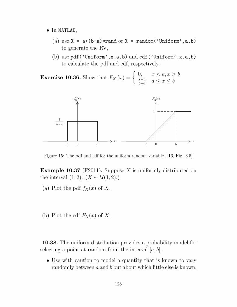
• In MATLAB,
(a) use X = a+(b-a)*rand or X = random(’Uniform’,a,b)
to generate the RV,
(b) use pdf(’Uniform’,x,a,b) and cdf(’Uniform’,x,a,b)
to calculate the pdf and cdf, respectively.
Exercise 10.36. Show that FX (x) =
0, x < a, x > bx−ab−a , a ≤ x ≤ b
84 Probability theory, random variables and random processes
x x0
b – a1
a b 0a b
1
fx(x) Fx(x)
Fig. 3.5 The pdf and cdf for the uniform random variable.
xμ
x0μ0
12πσ2
1
21
fx(x) Fx(x)
Fig. 3.6 The pdf and cdf of a Gaussian random variable.
Gaussian (or normal) random variable This is a continuous random variable thatis described by the following pdf:
fx(x) = 1√2πσ 2
exp
− (x− μ)2
2σ 2
, (3.16)
where μ and σ 2 are two parameters whose meaning is described later. It is usually denotedas N (μ, σ 2). Figure 3.6 shows sketches of the pdf and cdf of a Gaussian random variable.
The Gaussian random variable is the most important and frequently encountered ran-dom variable in communications. This is because thermal noise, which is the major sourceof noise in communication systems, has a Gaussian distribution. Gaussian noise and theGaussian pdf are discussed in more depth at the end of this chapter.
The problems explore other pdf models. Some of these arise when a random variableis passed through a nonlinearity. How to determine the pdf of the random variable in thiscase is discussed next.
Funct ions of a random variable A function of a random variable y = g(x) is itself arandom variable. From the definition, the cdf of y can be written as
Fy(y) = P(ω ∈ : g(x(ω)) ≤ y). (3.17)
Figure 15: The pdf and cdf for the uniform random variable. [16, Fig. 3.5]
Example 10.37 (F2011). Suppose X is uniformly distributed onthe interval (1, 2). (X ∼ U(1, 2).)
(a) Plot the pdf fX(x) of X.
(b) Plot the cdf FX(x) of X.
10.38. The uniform distribution provides a probability model forselecting a point at random from the interval [a, b].
• Use with caution to model a quantity that is known to varyrandomly between a and b but about which little else is known.
128

Example 10.39. [9, Ex. 4.1 p. 140-141] In coherent radio com-munications, the phase difference between the transmitter and thereceiver, denoted by Θ, is modeled as having a uniform density on[−π, π].
(a) P [Θ ≤ 0] = 12
(b) P[Θ ≤ π
2
]= 3
4
Exercise 10.40. Show that when X ∼ U([a, b]), EX = a+b2 ,
VarX = (b−a)2
12 , and E[X2]
= 13
(b2 + ab+ a2
).
10.4.2 Gaussian Distribution
10.41. This is the most widely used model for the distributionof a random variable. When you have many independent randomvariables, a fundamental result called the central limit theorem(CLT) (informally) says that the sum (technically, the average) ofthem can often be approximated by normal distribution.
Definition 10.42. Gaussian random variables:
(a) Often called normal random variables because they occur sofrequently in practice.
(b) In MATLAB, use X = random(’Normal’,m,σ) or X = σ*randn+ m.
(c) fX (x) = 1√2πσe−
12(
x−mσ )
2
.
• In Excel, use NORMDIST(x,m,σ,FALSE).In MATLAB, use normpdf(x,m,σ) or pdf(’Normal’,x,m,σ).
• Figure 16 displays the famous bell-shaped graph of theGaussian pdf. This curve is also called the normal curve.
129
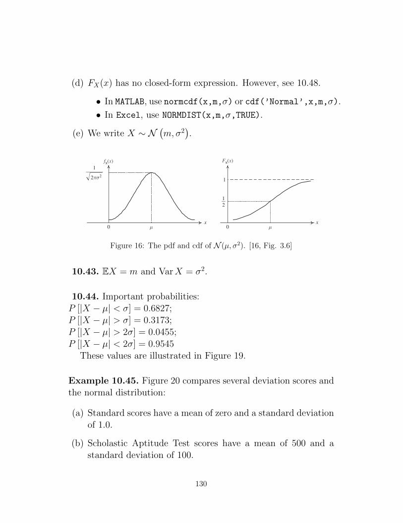
(d) FX(x) has no closed-form expression. However, see 10.48.
• In MATLAB, use normcdf(x,m,σ) or cdf(’Normal’,x,m,σ).
• In Excel, use NORMDIST(x,m,σ,TRUE).
(e) We write X ∼ N(m,σ2
).
84 Probability theory, random variables and random processes
x x0
b – a1
a b 0a b
1
fx(x) Fx(x)
Fig. 3.5 The pdf and cdf for the uniform random variable.
xμ
x0μ0
12πσ2
1
21
fx(x) Fx(x)
Fig. 3.6 The pdf and cdf of a Gaussian random variable.
Gaussian (or normal) random variable This is a continuous random variable thatis described by the following pdf:
fx(x) = 1√2πσ 2
exp
− (x− μ)2
2σ 2
, (3.16)
where μ and σ 2 are two parameters whose meaning is described later. It is usually denotedas N (μ, σ 2). Figure 3.6 shows sketches of the pdf and cdf of a Gaussian random variable.
The Gaussian random variable is the most important and frequently encountered ran-dom variable in communications. This is because thermal noise, which is the major sourceof noise in communication systems, has a Gaussian distribution. Gaussian noise and theGaussian pdf are discussed in more depth at the end of this chapter.
The problems explore other pdf models. Some of these arise when a random variableis passed through a nonlinearity. How to determine the pdf of the random variable in thiscase is discussed next.
Funct ions of a random variable A function of a random variable y = g(x) is itself arandom variable. From the definition, the cdf of y can be written as
Fy(y) = P(ω ∈ : g(x(ω)) ≤ y). (3.17)
Figure 16: The pdf and cdf of N (µ, σ2). [16, Fig. 3.6]
10.43. EX = m and VarX = σ2.
10.44. Important probabilities:P [|X − µ| < σ] = 0.6827;P [|X − µ| > σ] = 0.3173;P [|X − µ| > 2σ] = 0.0455;P [|X − µ| < 2σ] = 0.9545
These values are illustrated in Figure 19.
Example 10.45. Figure 20 compares several deviation scores andthe normal distribution:
(a) Standard scores have a mean of zero and a standard deviationof 1.0.
(b) Scholastic Aptitude Test scores have a mean of 500 and astandard deviation of 100.
130

109 3.5 The Gaussian random variable and process
0 0.2 0.4 0.6 0.8 1−0.8
−0.6
−0.4
−0.2
0
0.2
0.4
0.6
t (s)
Sign
al a
mpl
itude
(V
)
(a)
−1 −0.5 0 0.5 10
0.5
1
1.5
2
2.5
3
3.5
4
x (V)
f x(x
) (1
/V)
(b)
HistogramGaussian fitLaplacian fit
Fig. 3.14 (a) A sample skeletal muscle (emg) signal, and (b) its histogram and pdf fits.
1 =[∫ ∞
−∞fx(x)dx
]2
=[∫ ∞
−∞K1e−ax2
dx
]2
= K21
∫ ∞
x=−∞e−ax2
dx∫ ∞
y=−∞e−ay2
dy
= K21
∫ ∞
x=−∞
∫ ∞
y=−∞e−a(x2+y2)dxdy. (3.103)
Figure 17: Electrical activity of a skeletal muscle: (a) A sample skeletal muscle(emg) signal, and (b) its histogram and pdf fits. [16, Fig. 3.14]
131

111 3.5 The Gaussian random variable and process
−15 −10 −5 0 5 10 150
0.05
0.1
0.15
0.2
0.25
0.3
0.35
0.4
x
f x(x
)
σx = 1
σx = 2
σx = 5
Fig. 3.15 Plots of the zero-mean Gaussian pdf for different values of standard deviation, σx.
Table 3.1 Influence of σx on different quantities
Range (±kσx) k = 1 k = 2 k = 3 k = 4
P(mx − kσx < x ≤ mx + kσx) 0.683 0.955 0.997 0.999Error probability 10−3 10−4 10−6 10−8
Distance from the mean 3.09 3.72 4.75 5.61
of the pdf are ignorable. Indeed when communication systems are considered later it is the
presence of these tails that results in bit errors. The probabilities are on the order of 10−3–
10−12, very small, but still significant in terms of system performance. It is of interest to
see how far, in terms of σx, one must be from the mean value to have the different levels of
error probabilities. As shall be seen in later chapters this translates to the required SNR to
achieve a specified bit error probability. This is also shown in Table 3.1.
Having considered the single (or univariate) Gaussian random variable, we turn our
attention to the case of two jointly Gaussian random variables (or the bivariate case). Again
they are described by their joint pdf which, in general, is an exponential whose exponent
is a quadratic in the two variables, i.e., fx,y(x, y) = Ke(ax2+bx+cxy+dy+ey2+f ), where the con-
stants K, a, b, c, d, e, and f are chosen to satisfy the basic properties of a valid joint pdf,
namely being always nonnegative (≥ 0), having unit volume, and also that the marginal
pdfs, fx(x) = ∫∞−∞ fx,y(x, y)dy and fy(y) = ∫∞−∞ fx,y(x, y)dx, are valid. Written in standard
form the joint pdf is
Figure 18: Plots of the zero-mean Gaussian pdf for different values of standarddeviation, σX . [16, Fig. 3.15]
23) Fourier transform: ( ) ( )2 21
2j mj x
X Xf f x e dt eω ω σω
∞− −−
−∞
= =∫F .
24) Note that 2xe dxα π
α
∞−
−∞
=∫ .
25) [ ] x mP X x Qσ−⎛ ⎞> = ⎜ ⎟
⎝ ⎠; [ ] 1 x m xP X x Q Q
σ σ− −⎛ ⎞ ⎛< = − = −⎜ ⎟ ⎜
⎝ ⎠ ⎝m ⎞⎟⎠
.
• 0.6827, 0.3173P X P Xμ σ μ σ⎡ − < ⎤ = ⎡ − > ⎤ =⎣ ⎦ ⎣ ⎦
2 0.0455, 2 0.9545P X P Xμ σ μ σ⎡ − > ⎤ = ⎡ − < ⎤ =⎣ ⎦ ⎣ ⎦
μ σ+μ σ− μ
68%
( )Xf x
μ 2μ σ+ 2μ σ−
( )Xf x
95%
26) Q-function: ( )2
212
x
z
Q z e dxπ
∞−
= ∫ corresponds to [ ]P X z> where ;
that is
( )~ 0,1X N
( )Q z is the probability of the “tail” of ( )0,1N .
( )0,1N
z 0
( )Q z
0.5
a) Q is a decreasing function with ( ) 102
Q = .
b) ( ) ( )1Q z Q z− = −
c) ( )( )1 1Q Q z− − = z−
d) ( )2
22
2 sin
0
1 x
Q x e d
π
θ θπ
−= ∫ . ( )
2
24
2 2 sin
0
1 x
Q x e d
π
θ θπ
−= ∫ .
e) ( )2
212
xd Q x edx π
−= − ; ( )( )
( )( )( )
2
212
f xd dQ f x e f xdx dxπ
−= − .
Figure 19: Probability density function of X ∼ N (µ, σ2) .
6.1 Normal Probability DistributionsThe domain of bell-shaped distributions is the setof all real numbers.
6.2 The Standard Normal DistributionTo work with normal distributions, we need thestandard score.
6.3 Applications of Normal DistributionsThe normal distribution can help us to determineprobabilities.
6.4 NotationThe z notation is critical in the use of normaldistributions.
6.5 Normal Approximation of theBinomialBinomial probabilities can be estimated by usinga normal distribution.
6 Normal Probability Distributions
6.1 Normal Probability Distributions
Intelligence ScoresThe normal probability distribution is considered the single most important proba-bility distribution. An unlimited number of continuous random variables have either a normal
or an approximately normal distribution.
We are all familiar with IQ (intelligence quotient) scores and/or SAT (Scholastic Aptitude Test)scores. IQ scores have a mean of 100 and a standard deviation of 16. SAT scores have a mean of
500 with a standard deviation of 100. But did you know that these continuous random variables
also follow a normal distribution?
Figure A, pictures the comparison of sev-
eral deviation scores and the normal distri-
bution: Standard scores have a mean of
zero and a standard deviation of 1.0.
Scholastic Aptitude Test scores have a
mean of 500 and a standard deviation of
100.
Binet Intelligence Scale scores have a
mean of 100 and a standard deviation of 16.
In each case there are 34 percent of the
scores between the mean and one standard
deviation, 14 percent between one and two
standard deviations, and 2 percent beyond
two standard deviations.
Source: Beck, Applying Psychology: Critical and Creative Thinking, Figure 6.2 “Pictures the Comparison of Several DeviationScores and the Normal Distribution,” © 1992 Prentice-Hall, Inc. Reproduced by permission of Pearson Education, Inc.
–3.0 –2.0 –1.0 0
2% 2%14% 14%34% 34%
Standard Scores1.0 2.0 3.0
200 300 400 500SAT Scores
600 700 800
52 68 84 100Binet Intelligence Scale Scores
116 132 148
F IGURE A
© 2010/Jupiterimages Corporation
Cop
yrig
ht 2
010
Cen
gage
Lea
rnin
g. A
ll R
ight
s R
eser
ved.
May
not
be
copi
ed, s
cann
ed, o
r du
plic
ated
, in
who
le o
r in
par
t. D
ue to
ele
ctro
nic
righ
ts, s
ome
thir
d pa
rty
cont
ent m
ay b
e su
ppre
ssed
fro
m th
e eB
ook
and/
or e
Cha
pter
(s).
Edi
tori
al r
evie
w h
as d
eem
ed th
at a
ny s
uppr
esse
d co
nten
t doe
s no
t mat
eria
lly a
ffec
t the
ove
rall
lear
ning
exp
erie
nce.
Cen
gage
Lea
rnin
g re
serv
es th
e ri
ght t
o re
mov
e ad
ditio
nal c
onte
nt a
t any
tim
e if
sub
sequ
ent r
ight
s re
stri
ctio
ns r
equi
re it
.
Figure 20: Comparison of Several Deviation Scores and the Normal Distribution
132

(c) Binet Intelligence Scale41 scores have a mean of 100 and astandard deviation of 16.
In each case there are 34 percent of the scores between themean and one standard deviation, 14 percent between one andtwo standard deviations, and 2 percent beyond two standarddeviations. [Source: Beck, Applying Psychology: Critical andCreative Thinking.]
10.46. N (0, 1) is the standard Gaussian (normal) distribution.
• In Excel, use NORMSINV(RAND()).In MATLAB, use randn.
• The standard normal cdf is denoted by Φ(z).
It inherits all properties of cdf.
Moreover, note that Φ(−z) = 1− Φ(z).
10.47. Relationship between N (0, 1) and N (m,σ2).
(a) An arbitrary Gaussian random variable with mean m andvariance σ2 can be represented as σZ+m, where Z ∼ N (0, 1).
41Alfred Binet, who devised the first general aptitude test at the beginning of the 20thcentury, defined intelligence as the ability to make adaptations. The general purpose of thetest was to determine which children in Paris could benefit from school. Binets test, like itssubsequent revisions, consists of a series of progressively more difficult tasks that children ofdifferent ages can successfully complete. A child who can solve problems typically solved bychildren at a particular age level is said to have that mental age. For example, if a child cansuccessfully do the same tasks that an average 8-year-old can do, he or she is said to have amental age of 8. The intelligence quotient, or IQ, is defined by the formula:
IQ = 100 × (Mental Age/Chronological Age)
There has been a great deal of controversy in recent years over what intelligence tests measure.Many of the test items depend on either language or other specific cultural experiences forcorrect answers. Nevertheless, such tests can rather effectively predict school success. Ifschool requires language and the tests measure language ability at a particular point of timein a childs life, then the test is a better-than-chance predictor of school performance.
133
This relationship can be used to generate general GaussianRV from standard Gaussian RV.
(b) If X ∼ N(m,σ2
), the random variable
Z =X −mσ
is a standard normal random variable. That is, Z ∼ N (0, 1).
• Creating a new random variable by this transformationis referred to as standardizing.
• The standardized variable is called “standard score” or“z-score”.
10.48. It is impossible to express the integral of a Gaussian PDFbetween non-infinite limits (e.g., (20)) as a function that appearson most scientific calculators.
• An old but still popular technique to find integrals of theGaussian PDF is to refer to tables that have been obtainedby numerical integration.
One such table is the table that lists Φ(z) for many valuesof positive z.
For X ∼ N(m,σ2
), we can show that the CDF of X can
be calculated by
FX(x) = Φ
(x−mσ
).
Example 10.49. Suppose Z ∼ N (0, 1). Evaluate the followingprobabilities.
(a) P [−1 ≤ Z ≤ 1]
134

(b) P [−2 ≤ Z ≤ 2]
Example 10.50. Suppose X ∼ N (1, 2). Find P [1 ≤ X ≤ 2].
10.51. Q-function : Q (z) =∞∫z
1√2πe−
x2
2 dx corresponds to P [X > z]
where X ∼ N (0, 1); that is Q (z) is the probability of the “tail”of N (0, 1). The Q function is then a complementary cdf (ccdf).
( )0,1N
z 0
( )Q z
-3 -2 -1 0 1 2 30
0.1
0.2
0.3
0.4
0.5
0.6
0.7
0.8
0.9
1
z
10,2
⎛ ⎞⎜ ⎟⎝ ⎠
N
z
( )erf z
0
( )2Q z
Figure 21: Q-function
(a) Q is a decreasing function with Q (0) = 12 .
(b) Q (−z) = 1−Q (z) = Φ(z)
10.52. Error function (MATLAB): erf (z) = 2√π
z∫0
e−x2
dx =
1− 2Q(√
2z)
(a) It is an odd function of z.
(b) For z ≥ 0, it corresponds to P [|X| < z] where X ∼ N(0, 1
2
).
(c) limz→∞
erf (z) = 1
135

(d) erf (−z) = −erf (z)
(e) Φ(x) = 12
(1 + erf
(x√(2)
))= 1
2erfc(− x√
2
)(f) The complementary error function:
erfc (z) = 1− erf (z) = 2Q(√
2z)
= 2√π
∫∞z e−x
2
dx
f) ( )( ) ( ) ( )( ) ( )( )( )
( ) ( )2
212
f x x
a
dQ f x g x dx Q f x g x dx e f x g t dt dxdxπ
− ⎛ ⎞⎛ ⎞= + ⎜ ⎟⎜ ⎟⎝ ⎠⎝ ⎠
∫ ∫ ∫ ∫ .
g) Approximation:
i) ( )( )
2
22
1 121
z
Q z ea z a z b π
−⎡ ⎤⎢ ⎥≈⎢ ⎥− + +⎣ ⎦
; 1aπ
= , 2b π=
ii) ( )
22
22
2
1 1122
xxe Q x e
x x π
−−⎛ ⎞− ≤ ≤⎜ ⎟
⎝ ⎠.
27) Moment and central moment
n 0 1 2 3 4
nXE 1 μ 2 2μ σ+ ( )2 23μ μ σ+ 4 2 26 3 4μ μ σ σ+ +
( )nX μ⎡ −⎣E ⎤⎦ 1 0 2σ 0 43σ
• ( ) ( ) ( ) ( )2 0, odd
11 3 5 1 , even
k kk
kX k X
k kμ μ
σ− ⎧⎡ ⎤ ⎡ ⎤− = − − = ⎨⎣ ⎦ ⎣ ⎦ ⋅ ⋅ ⋅ ⋅ −⎩
E E
• ( )
( )
22 4 6 1 , odd
1 3 5 1 , even
kk
k
k kX
k k
σμ π
σ
⎧⋅ ⋅ ⋅ ⋅ −⎪⎡ ⎤− = ⎨⎣ ⎦ ⎪ ⋅ ⋅ ⋅ ⋅ −⎩
E [Papoulis p 111].
• 2 2 2Var 4 2X 4μ σ σ⎡ ⎤ = +⎣ ⎦ .
28) For ( )0,1N and , 1k ≥ ( ) ( )2 0, odd
11 3 5 1 , even
k k kX k X
k k− ⎧
⎡ ⎤ ⎡ ⎤= − = ⎨⎣ ⎦ ⎣ ⎦ ⋅ ⋅ ⋅ ⋅ −⎩E E
29) Error function (Matlab): ( ) (2
0
2 1 2 2z
xerf z e dx Q zπ
−= = −∫ ) corresponds to
P X z⎡ <⎣ ⎤⎦ where X ~ 10,2
⎛ ⎞⎜ ⎟⎝ ⎠
N .
10,2
⎛ ⎞⎜ ⎟⎝ ⎠
N
z
( )erf z
0
( )2Q z
a) ( )lim 1
zerf z
→∞=
b) ( ) (erf z erf z− = − )Figure 22: erf-function and Q-function
10.4.3 Exponential Distribution
Definition 10.53. The exponential distribution is denoted byE (λ).
(a) λ > 0 is a parameter of the distribution, often called the rateparameter.
(b) Characterized by
• fX (x) =
λe−λx, x > 0,0, x ≤ 0
• FX (x) =
1− e−λx, x > 0,0, x ≤ 0
136

• Survival-, survivor-, or reliability-function:
(c) MATLAB:
• X = exprnd(1/λ) or random(’exp’,1/λ)
• fX(x) = exppdf(x,1/λ) or pdf(’exp’,x,1/λ)
• FX(x) = expcdf(x,1/λ) or cdf(’exp’,x,1/λ)
Example 10.54. Suppose X ∼ E(λ), find P [1 < X < 2].
Exercise 10.55. Exponential random variable as a continuousversion of geometric random variable: Suppose X ∼ E (λ). Showthat bXc ∼ G0(e
−λ) and dXe ∼ G1(e−λ)
Example 10.56. The exponential distribution is intimately re-lated to the Poisson process. It is often used as a probabilitymodel for the (waiting) time until a “rare” event occurs.
• time elapsed until the next earthquake in a certain region
• decay time of a radioactive particle
• time between independent events such as arrivals at a servicefacility or arrivals of customers in a shop.
• duration of a cell-phone call
• time it takes a computer network to transmit a message fromone node to another.
137

10.57. EX = 1λ
Example 10.58. Phone Company A charges $0.15 per minutefor telephone calls. For any fraction of a minute at the end ofa call, they charge for a full minute. Phone Company B alsocharges $0.15 per minute. However, Phone Company B calculatesits charge based on the exact duration of a call. If T , the durationof a call in minutes, is exponential with parameter λ = 1/3, whatare the expected revenues per call E [RA] and E [RB] for companiesA and B?
Solution : First, note that ET = 1λ = 3. Hence,
E [RB] = E [0.15× T ] = 0.15ET = $0.45.
andE [RA] = E [0.15× dT e] = 0.15E dT e .
Now, recall, from Exercise 10.55, that dT e ∼ G1
(e−λ). Hence,
E dT e = 11−e−λ ≈ 3.53. Therefore,
E [RA] = 0.15E dT e ≈ 0.5292.
10.59. Memoryless property : The exponential r.v. is the onlycontinuous42 r.v. on [0,∞) that satisfies the memoryless property:
P [X > s+ x |X > s ] = P [X > x]
for all x > 0 and all s > 0 [18, p. 157–159]. In words, the futureis independent of the past. The fact that it hasn’t happened yet,tells us nothing about how much longer it will take before it doeshappen.
• Imagining that the exponentially distributed random variableX represents the lifetime of an item, the residual life of an itemhas the same exponential distribution as the original lifetime,
42For discrete random variable, geometric random variables satisfy the memoryless property.
138

regardless of how long the item has been already in use. Inother words, there is no deterioration/degradation over time.If it is still currently working after 20 years of use, then today,its condition is “just like new”.
• In particular, suppose we define the setB+x to be x+ b : b ∈ B.For any x > 0 and set B ⊂ [0,∞), we have
P [X ∈ B + x|X > x] = P [X ∈ B]
because
P [X ∈ B + x]
P [X > x]=
∫B+x λe
−λtdt
e−λxτ=t−x
=
∫B λe
−λ(τ+x)dτ
e−λx.
10.5 Function of Continuous Random Variables: SISO
Reconsider the derived random variable Y = g(X).
Recall that we can find EY easily by (22):
EY = E [g(X)] =
∫Rg(x)fX(x)dx.
However, there are cases when we have to evaluate probabilitydirectly involving the random variable Y or find fY (y) directly.
Recall that for discrete random variables, it is easy to find pY (y)by adding all pX(x) over all x such that g(x) = y:
pY (y) =∑
x:g(x)=y
pX(x). (23)
For continuous random variables, it turns out that we can’t43 sim-ply integrate the pdf of X to get the pdf of Y .
43When you applied Equation (23) to continuous random variables, what you would get is0 = 0, which is true but not interesting nor useful.
139

10.60. For Y = g(X), if you want to find fY (y), the followingtwo-step procedure will always work and is easy to remember:
(a) Find the cdf FY (y) = P [Y ≤ y].
(b) Compute the pdf from the cdf by “finding the derivative”fY (y) = d
dyFY (y) (as described in 10.13).
10.61. Linear Transformation : Suppose Y = aX + b. Then,the cdf of Y is given by
FY (y) = P [Y ≤ y] = P [aX + b ≤ y] =
P[X ≤ y−b
a
], a > 0,
P[X ≥ y−b
a
], a < 0.
Now, by definition, we know that
P
[X ≤ y − b
a
]= FX
(y − ba
),
and
P
[X ≥ y − b
a
]= P
[X >
y − ba
]+ P
[X =
y − ba
]= 1− FX
(y − ba
)+ P
[X =
y − ba
].
For continuous random variable, P[X = y−b
a
]= 0. Hence,
FY (y) =
FX
(y−ba
), a > 0,
1− FX(y−ba
), a < 0.
Finally, fundamental theorem of calculus and chain rule gives
fY (y) =d
dyFY (y) =
1afX
(y−ba
), a > 0,
−1afX
(y−ba
), a < 0.
Note that we can further simplify the final formula by using the| · | function:
fY (y) =1
|a|fX(y − ba
), a 6= 0. (24)
140

Graphically, to get the plots of fY , we compress fX horizontallyby a factor of a, scale it vertically by a factor of 1/|a|, and shift itto the right by b.
Of course, if a = 0, then we get the uninteresting degeneratedrandom variable Y ≡ b.
10.62. SupposeX ∼ N (m,σ2) and Y = aX+b for some constantsa and b. Then, we can use (24) to show that X ∼ N (am+b, a2σ2).
Example 10.63. Amplitude modulation in certain communica-tion systems can be accomplished using various nonlinear devicessuch as a semiconductor diode. Suppose we model the nonlineardevice by the function Y = X2. If the input X is a continuousrandom variable, find the density of the output Y = X2.
141

Exercise 10.64 (F2011). Suppose X is uniformly distributed onthe interval (1, 2). (X ∼ U(1, 2).) Let Y = 1
X2 .
(a) Find fY (y).
(b) Find EY .
Exercise 10.65 (F2011). Consider the function
g(x) =
x, x ≥ 0−x, x < 0.
Suppose Y = g(X), where X ∼ U(−2, 2).Remark: The function g operates like a full-wave rectifier in
that if a positive input voltage X is applied, the output is Y = X,while if a negative input voltage X is applied, the output is Y =−X.
(a) Find EY .
(b) Plot the cdf of Y .
(c) Find the pdf of Y
142

Discrete ContinuousP [X ∈ B] =
∑x∈B
pX(x)∫B
fX(x)dx
P [X = x] = pX(x) = F (x)− F (x−) 0
Interval prob.
PX ((a, b]) = F (b)− F (a)
PX ([a, b]) = F (b)− F(a−)
PX ([a, b)) = F(b−)− F
(a−)
PX ((a, b)) = F(b−)− F (a)
PX ((a, b]) = PX ([a, b])
= PX ([a, b)) = PX ((a, b))
=
b∫a
fX(x)dx = F (b)− F (a)
EX =∑x
xpX(x)+∞∫−∞
xfX(x)dx
For Y = g(X), pY (y) =∑
x: g(x)=y
pX(x)
fY (y) =d
dyP [g(X) ≤ y] .
Alternatively,
fY (y) =∑k
fX(xk)
|g′(xk)|,
xk are the real-valued rootsof the equation y = g(x).
For Y = g(X),P [Y ∈ B] =
∑x:g(x)∈B
pX(x)∫
x:g(x)∈BfX(x)dx
E [g(X)] =∑x
g(x)pX(x)+∞∫−∞
g(x)fX(x)dx
E [X2] =∑x
x2pX(x)+∞∫−∞
x2fX(x)dx
VarX =∑x
(x− EX)2pX(x)+∞∫−∞
(x− EX)2 fX(x)dx
Table 4: Important Formulas for Discrete and Continuous Random Variables
143

Sirindhorn International Institute of Technology
Thammasat University
School of Information, Computer and Communication Technology
ECS315 2013/1 Part V.1 Dr.Prapun
11 Multiple Random Variables
One is often interested not only in individual random variables, butalso in relationships between two or more random variables. Fur-thermore, one often wishes to make inferences about one randomvariable on the basis of observations of other random variables.
Example 11.1. If the experiment is the testing of a new medicine,the researcher might be interested in cholesterol level, blood pres-sure, and the glucose level of a test person.
11.1 A Pair of Discrete Random Variables
In this section, we consider two discrete random variables, say Xand Y , simultaneously.
11.2. The analysis are different from Section 9.2 in two mainaspects. First, there may be no deterministic relationship (such asY = g(X)) between the two random variables. Second, we wantto look at both random variables as a whole, not just X alone orY alone.
Example 11.3. Communication engineers may be interested inthe input X and output Y of a communication channel.
144

Example 11.4. Of course, to rigorously define (any) random vari-ables, we need to go back to the sample space Ω. Recall Example7.4 where we considered several random variables defined on thesample space Ω = 1, 2, 3, 4, 5, 6 where the outcomes are equallylikely. In that example, we define X(ω) = ω and Y (ω) = (ω− 3)2.
Example 11.5. Consider the scores of 20 students below:
10, 9, 10, 9, 9, 10, 9, 10, 10, 9︸ ︷︷ ︸Room #1
, 1, 3, 4, 6, 5, 5, 3, 3, 1, 3.︸ ︷︷ ︸Room #2
The first ten scores are from (ten) students in room #1. The last10 scores are from (ten) students in room #2.
Suppose we have the a score report card for each student. Then,in total, we have 20 report cards.
Figure 23: In Example 11.5, we pick a report card randomly from a pile ofcards.
I pick one report card up randomly. Let X be the score on thatcard.
• What is the chance that X > 5? (Ans: P [X > 5] = 11/20.)
145
• What is the chance thatX = 10? (Ans: pX(10) = P [X = 10] =5/20 = 1/4.)
Now, let the random variable Y denote the room# of the studentwhose report card is picked up.
• What is the probability that X = 10 and Y = 2?
• What is the probability that X = 10 and Y = 1?
• What is the probability that X > 5 and Y = 1?
• What is the probability that X > 5 and Y = 2?
Now suppose someone informs me that the report card which Ipicked up is from a student in room #1. (He may be able to tellthis by the color of the report card of which I have no knowledge.)I now have an extra information that Y = 1.
• What is the probability that X > 5 given that Y = 1?
• What is the probability that X = 10 given that Y = 1?
146
11.6. Recall that, in probability, “,” means “and”. For example,
P [X = x, Y = y] = P [X = x and Y = y]
and
P [3 ≤ X < 4, Y < 1] = P [3 ≤ X < 4 and Y < 1]
= P [X ∈ [3, 4) and Y ∈ (−∞, 1)] .
In general,
[“Some condition(s) on X”,“Some condition(s) on Y ”]
is the same as the intersection of the individual statements:
[“Some condition(s) on X”] ∩ [“Some condition(s) on Y ”]
which simply means both statements happen.More technically,
[X ∈ B, Y ∈ C] = [X ∈ B and Y ∈ C] = [X ∈ B] ∩ [Y ∈ C]
andP [X ∈ B, Y ∈ C] = P [X ∈ B and Y ∈ C]
= P ([X ∈ B] ∩ [Y ∈ C]) .
Remark: Linking back to the original sample space, this short-hand actually says
[X ∈ B, Y ∈ C] = [X ∈ B and Y ∈ C]
= ω ∈ Ω : X(ω) ∈ B and Y (ω) ∈ C= ω ∈ Ω : X(ω) ∈ B ∩ ω ∈ Ω : Y (ω) ∈ C= [X ∈ B] ∩ [Y ∈ C] .
147

11.7. The concept of conditional probability can be straightfor-wardly applied to discrete random variables. For example,
P [“Some condition(s) on X” | “Some condition(s) on Y ”] (25)
is the conditional probability P (A|B) where
A = [“Some condition(s) on X”] and
B = [“Some condition(s) on Y ”].
Recall that P (A|B) = P (A ∩B)/P (B). Therefore,
P [X = x|Y = y] =P [X = x and Y = y]
P [Y = y],
and
P [3 ≤ X < 4|Y < 1] =P [3 ≤ X < 4 and Y < 1]
P [Y < 1]
More generally, (25) is
=P ([“Some condition(s) on X”] ∩ [“Some condition(s) on Y ”])
P ([“Some condition(s) on Y ”])
=P ([“Some condition(s) on X”,“Some condition(s) on Y ”])
P ([“Some condition(s) on Y ”])
=P [“Some condition(s) on X”,“Some condition(s) on Y ”]
P [“Some condition(s) on Y ”]
More technically,
P [X ∈ B|Y ∈ C] = P ([X ∈ B] |[Y ∈ C]) =P ([X ∈ B] ∩ [Y ∈ C])
P ([Y ∈ C])
=P [X ∈ B, Y ∈ C]
P [Y ∈ C].
148

Definition 11.8. Joint pmf : If X and Y are two discrete ran-dom variables (defined on a same sample space with probabilitymeasure P ), the function pX,Y (x, y) defined by
pX,Y (x, y) = P [X = x, Y = y]
is called the joint probability mass function of X and Y .
(a) We can visualize the joint pmf via stem plot. See Figure 24.
(b) To evaluate the probability for a statement that involves bothX and Y random variables:
We first find all pairs (x, y) that satisfy the condition(s) inthe statement, and then add up all the corresponding valuesjoint pmf.
More technically, we can then evaluate P [(X, Y ) ∈ R] by
P [(X, Y ) ∈ R] =∑
(x,y):(x,y)∈RpX,Y (x, y).
Example 11.9 (F2011). Consider random variables X and Ywhose joint pmf is given by
pX,Y (x, y) =
c (x+ y) , x ∈ 1, 3 and y ∈ 2, 4 ,0, otherwise.
(a) Check that c = 1/20.
(b) Find P[X2 + Y 2 = 13
].
In most situation, it is much more convenient to focus on the“important” part of the joint pmf. To do this, we usually presentthe joint pmf (and the conditional pmf) in their matrix forms:
149
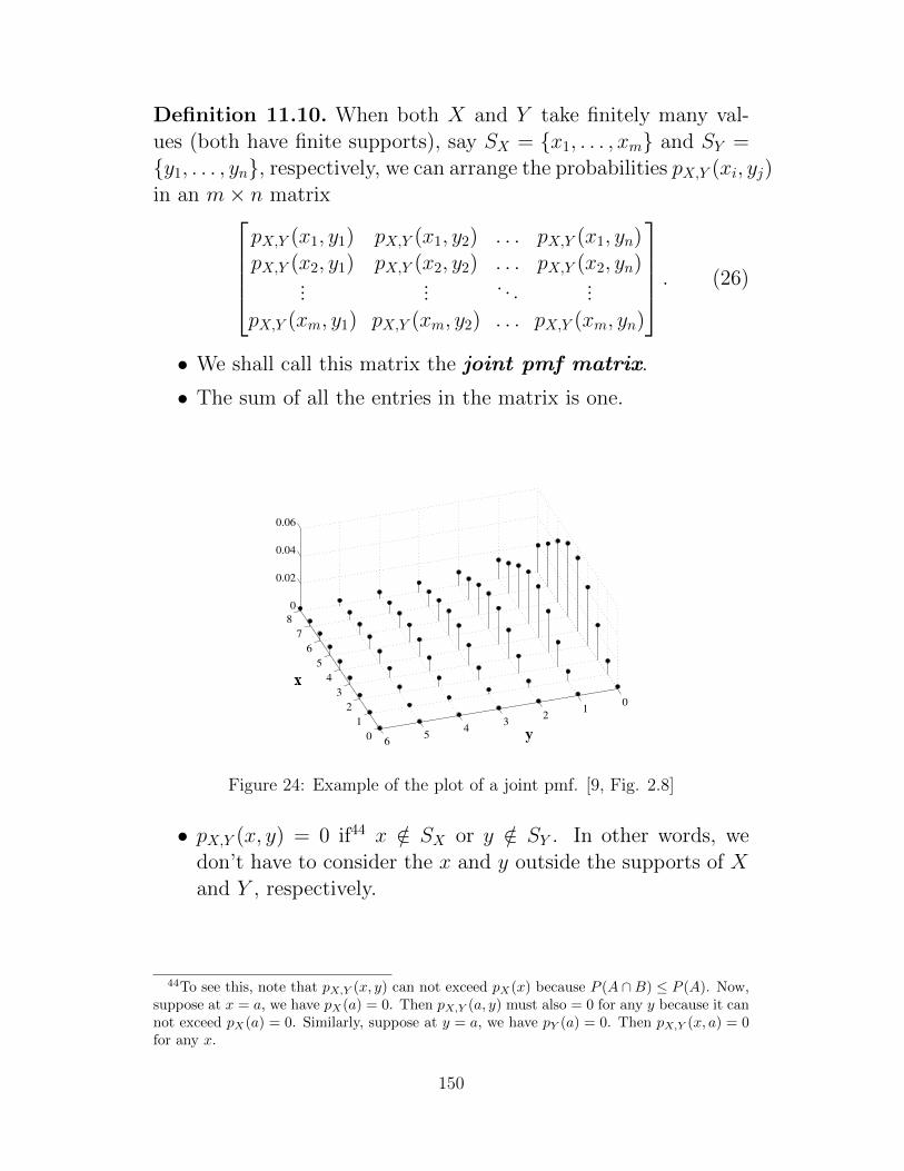
Definition 11.10. When both X and Y take finitely many val-ues (both have finite supports), say SX = x1, . . . , xm and SY =y1, . . . , yn, respectively, we can arrange the probabilities pX,Y (xi, yj)in an m× n matrix
pX,Y (x1, y1) pX,Y (x1, y2) . . . pX,Y (x1, yn)pX,Y (x2, y1) pX,Y (x2, y2) . . . pX,Y (x2, yn)
...... . . . ...
pX,Y (xm, y1) pX,Y (xm, y2) . . . pX,Y (xm, yn)
. (26)
• We shall call this matrix the joint pmf matrix.
• The sum of all the entries in the matrix is one.
2.3 Multiple random variables 75
Example 2.13. In the preceding example, what is the probability that the first cache
miss occurs after the third memory access?
Solution. We need to find
P(T > 3) =∞
∑k=4
P(T = k).
However, since P(T = k) = 0 for k ≤ 0, a finite series is obtained by writing
P(T > 3) = 1−P(T ≤ 3)
= 1−3
∑k=1
P(T = k)
= 1− (1− p)[1+ p+ p2].
Joint probability mass functions
The joint probability mass function of X and Y is defined by
pXY (xi,y j) := P(X = xi,Y = y j). (2.7)
An example for integer-valued random variables is sketched in Figure 2.8.
0
1
2
3
4
5
6
7
8
01
23
45
6
0
0.02
0.04
0.06
ji
Figure 2.8. Sketch of bivariate probability mass function pXY (i, j).
It turns out that we can extract the marginal probability mass functions pX (xi) and
pY (y j) from the joint pmf pXY (xi,y j) using the formulas
pX (xi) = ∑j
pXY (xi,y j) (2.8)
Figure 24: Example of the plot of a joint pmf. [9, Fig. 2.8]
• pX,Y (x, y) = 0 if44 x /∈ SX or y /∈ SY . In other words, wedon’t have to consider the x and y outside the supports of Xand Y , respectively.
44To see this, note that pX,Y (x, y) can not exceed pX(x) because P (A ∩B) ≤ P (A). Now,suppose at x = a, we have pX(a) = 0. Then pX,Y (a, y) must also = 0 for any y because it cannot exceed pX(a) = 0. Similarly, suppose at y = a, we have pY (a) = 0. Then pX,Y (x, a) = 0for any x.
150
11.11. From the joint pmf, we can find pX(x) and pY (y) by
pX(x) =∑y
pX,Y (x, y) (27)
pY (y) =∑x
pX,Y (x, y) (28)
In this setting, pX(x) and pY (y) are call the marginal pmfs (todistinguish them from the joint one).
(a) Suppose we have the joint pmf matrix in (26). Then, the sumof the entries in the ith row is45 pX(xi), andthe sum of the entries in the jth column is pY (yj):
pX(xi) =n∑j=1
pX,Y (xi, yj) and pY (yj) =m∑i=1
pX,Y (xi, yj)
(b) In MATLAB, suppose we save the joint pmf matrix as P XY, thenthe marginal pmf (row) vectors p X and p Y can be found by
p_X = (sum(P_XY,2))’
p_Y = (sum(P_XY,1))
Example 11.12. Consider the following joint pmf matrix
45To see this, we consider A = [X = xi] and a collection defined by Bj = [Y = yj ]and B0 = [Y /∈ SY ]. Note that the collection B0, B1, . . . , Bn partitions Ω. So, P (A) =∑nj=0 P (A ∩Bj). Of course, because the support of Y is SY , we have P (A∩B0) = 0. Hence,
the sum can start at j = 1 instead of j = 0.
151

Definition 11.13. The conditional pmf of X given Y is definedas
pX|Y (x|y) = P [X = x|Y = y]
which gives
pX,Y (x, y) = pX|Y (x|y)pY (y) = pY |X(y|x)pX(x). (29)
11.14. Equation (29) is quite important in practice. In mostcases, systems are naturally defined/given/studied in terms of theirconditional probabilities, say pY |X(y|x). Therefore, it is importantthe we know how to construct the joint pmf from the conditionalpmf.
Example 11.15. Consider a binary symmetric channel. Supposethe input X to the channel is Bernoulli(0.3). At the output Y ofthis channel, the crossover (bit-flipped) probability is 0.1. Findthe joint pmf pX,Y (x, y) of X and Y .
Exercise 11.16. Toss-and-Roll Game:
Step 1 Toss a fair coin. Define X by
X =
1, if result = H,0, if result = T.
Step 2 You have two dice, Dice 1 and Dice 2. Dice 1 is fair. Dice 2 isunfair with p(1) = p(2) = p(3) = 2
9 and p(4) = p(5) = p(6) =19 .
(i) If X = 0, roll Dice 1.
(ii) If X = 1, roll Dice 2.
152

Record the result as Y .
Find the joint pmf pX,Y (x, y) of X and Y .
Exercise 11.17 (F2011). Continue from Example 11.9. Randomvariables X and Y have the following joint pmf
pX,Y (x, y) =
c (x+ y) , x ∈ 1, 3 and y ∈ 2, 4 ,0, otherwise.
(a) Find pX(x).
(b) Find EX.
(c) Find pY |X(y|1). Note that your answer should be of the form
pY |X(y|1) =
?, y = 2,?, y = 4,0, otherwise.
(d) Find pY |X(y|3).
Definition 11.18. The joint cdf of X and Y is defined by
FX,Y (x, y) = P [X ≤ x, Y ≤ y] .
153

Definition 11.19. Two random variables X and Y are said to beidentically distributed if, for every B, P [X ∈ B] = P [Y ∈ B].
Example 11.20. Let X ∼ Bernoulli(p). Let Y = X and Z = 1−X. Then, all of these random variables are identically distributed.
11.21. The following statements are equivalent:
(a) Random variables X and Y are identically distributed .
(b) For every B, P [X ∈ B] = P [Y ∈ B]
(c) pX(c) = pY (c) for all c
(d) FX(c) = FY (c) for all c
Definition 11.22. Two random variables X and Y are said to beindependent if the events [X ∈ B] and [Y ∈ C] are independentfor all sets B and C.
11.23. The following statements are equivalent:
(a) Random variables X and Y are independent .
(b) [X ∈ B] |= [Y ∈ C] for all B,C.
(c) P [X ∈ B, Y ∈ C] = P [X ∈ B]× P [Y ∈ C] for all B,C.
(d) pX,Y (x, y) = pX(x)× pY (y) for all x, y.
(e) FX,Y (x, y) = FX(x)× FY (y) for all x, y.
Definition 11.24. Two random variables X and Y are said to beindependent and identically distributed (i.i.d.) if X andY are both independent and identically distributed.
11.25. Being identically distributed does not imply independence.Similarly, being independent, does not imply being identically dis-tributed.
154

Example 11.26. Roll a dice. Let X be the result. Set Y = X.
Example 11.27. Suppose the pmf of a random variable X is givenby
pX (x) =
1/4, x = 3,α, x = 4,0, otherwise.
Let Y be another random variable. Assume that X and Y arei.i.d.
Find
(a) α,
(b) the pmf of Y , and
(c) the joint pmf of X and Y .
155
Example 11.28. Consider a pair of random variables X and Ywhose joint pmf is given by
pX,Y (x, y) =
1/15, x = 3, y = 1,2/15, x = 4, y = 1,4/15, x = 3, y = 3,β, x = 4, y = 3,0, otherwise.
(a) Are X and Y identically distributed?
(b) Are X and Y independent?
156

11.2 Extending the Definitions to Multiple RVs
Definition 11.29. Joint pmf:
pX1,X2,...,Xn(x1, x2, . . . , xn) = P [X1 = x1, X2 = x2, . . . , Xn = xn] .
Joint cdf:
FX1,X2,...,Xn(x1, x2, . . . , xn) = P [X1 ≤ x1, X2 ≤ x2, . . . , Xn ≤ xn] .
11.30. Marginal pmf:
Definition 11.31. Identically distributed random variables:The following statements are equivalent.
(a) Random variables X1, X2, . . . are identically distributed
(b) For every B, P [Xj ∈ B] does not depend on j.
(c) pXi(c) = pXj
(c) for all c, i, j.
(d) FXi(c) = FXj
(c) for all c, i, j.
Definition 11.32. Independence among finite number of ran-dom variables: The following statements are equivalent.
(a) X1, X2, . . . , Xn are independent
(b) [X1 ∈ B1], [X2 ∈ B2], . . . , [Xn ∈ Bn] are independent, for allB1, B2, . . . , Bn.
(c) P [Xi ∈ Bi,∀i] =∏n
i=1 P [Xi ∈ Bi], for all B1, B2, . . . , Bn.
(d) pX1,X2,...,Xn(x1, x2, . . . , xn) =
∏ni=1 pXi
(xi) for all x1, x2, . . . , xn.
(e) FX1,X2,...,Xn(x1, x2, . . . , xn) =
∏ni=1 FXi
(xi) for all x1, x2, . . . , xn.
Example 11.33. Toss a coin n times. For the ith toss, let
Xi =
1, if H happens on the ith toss,0, if T happens on the ith toss.
We then have a collection of i.i.d. random variablesX1, X2, X3, . . . , Xn.
157

Example 11.34. Roll a dice n times. Let Ni be the result of theith roll. We then have another collection of i.i.d. random variablesN1, N2, N3, . . . , Nn.
Example 11.35. Let X1 be the result of tossing a coin. Set X2 =X3 = · · · = Xn = X1.
11.36. If X1, X2, . . . , Xn are independent, then so is any subcol-lection of them.
11.37. For i.i.d. Xi ∼ Bernoulli(p), Y = X1 + X2 + · · · + Xn isB(n, p).
Definition 11.38. A pairwise independent collection of ran-dom variables is a collection of random variables any two of whichare independent.
(a) Any collection of (mutually) independent random variables ispairwise independent
(b) Some pairwise independent collections are not independent.See Example (11.39).
Example 11.39. Let suppose X, Y , and Z have the followingjoint probability distribution: pX,Y,Z (x, y, z) = 1
4 for (x, y, z) ∈(0, 0, 0), (0, 1, 1), (1, 0, 1), (1, 1, 0). This, for example, can be con-structed by starting with independent X and Y that are Bernoulli-12 . Then set Z = X ⊕ Y = X + Y mod 2.
(a) X, Y, Z are pairwise independent.
(b) X, Y, Z are not independent.
158

Sirindhorn International Institute of Technology
Thammasat University
School of Information, Computer and Communication Technology
ECS315 2013/1 Part V.2 Dr.Prapun
11.3 Function of Discrete Random Variables
11.40. Recall that for discrete random variable X, the pmf of aderived random variable Y = g(X) is given by
pY (y) =∑
x:g(x)=y
pX(x).
Similarly, for discrete random variables X and Y , the pmf of aderived random variable Z = g(X, Y ) is given by
pZ(z) =∑
(x,y):g(x,y)=z
pX,Y (x, y).
Example 11.41. Suppose the joint pmf of X and Y is given by
pX,Y (x, y) =
1/15, x = 0, y = 0,2/15, x = 1, y = 0,4/15, x = 0, y = 1,8/15, x = 1, y = 1,0, otherwise.
Let Z = X + Y . Find the pmf of Z.
159

Exercise 11.42 (F2011). Continue from Exercise 11.9. Let Z =X + Y .
(a) Find the pmf of Z.
(b) Find EZ.
11.43. In general, when Z = X + Y ,
pZ(z) =∑
(x,y):x+y=z
pX,Y (x, y)
=∑y
pX,Y (z − y, y) =∑x
pX,Y (x, z − x).
Furthermore, if X and Y are independent,
pZ(z) =∑
(x,y):x+y=z
pX (x) pY (y) (30)
=∑y
pX (z − y) pY (y) =∑x
pX (x) pY (z − x). (31)
Example 11.44. Suppose Λ1 ∼ P(λ1) and Λ2 ∼ P(λ2) are inde-pendent. Let Λ = Λ1+Λ2. Use (31) to show46 that Λ ∼ P(λ1+λ2).
First, note that pΛ(`) would be positive only on nonnegativeintegers because a sum of nonnegative integers (Λ1 and Λ2) is stilla nonnegative integer. So, the support of Λ is the same as thesupport for Λ1 and Λ2. Now, we know, from (31), that
P [Λ = `] = P [Λ1 + Λ2 = `] =∑i
P [Λ1 = i]P [Λ2 = `− i]
Of course, we are interested in ` that is a nonnegative integer.The summation runs over i = 0, 1, 2, . . .. Other values of i wouldmake P [Λ1 = i] = 0. Note also that if i > `, then ` − i < 0 andP [Λ2 = `− i] = 0. Hence, we conclude that the index i can only
46Remark: You may feel that simplifying the sum in this example (and in Exercise 11.45is difficult and tedious, in Section 13, we will introduce another technique which will makethe answer obvious. The idea is to realize that (31) is a convolution and hence we can useFourier transform to work with a product in another domain.
160

be integers from 0 to k:
P [Λ = `] =∑i=0
e−λ1λi1i!e−λ2
λ`−i2
(`− i)!
= e−(λ1+λ2) 1
`!
∑i=0
`!
i! (`− i)!λi1λ
`−i2
= e−(λ1+λ2) 1
`!
∑i=0
λi1λ`−i2 = e−(λ1+λ2) (λ1 + λ2)
`
`!,
where the last equality is from the binomial theorem. Hence, thesum of two independent Poisson random variables is still Poisson!
pΛ (`) =
e−(λ1+λ2) (λ1+λ2)
`
`! , ` ∈ 0, 1, 2, . . .0, otherwise
Exercise 11.45. Suppose B1 ∼ B(n1, p) and B2 ∼ B(n2, p) areindependent. Let B = B1 + B2. Use (31) to show that B ∼B(n1 + n2, p).
11.4 Expectation of Function of Discrete Random Vari-ables
11.46. Recall that the expected value of “any” function g of adiscrete random variable X can be calculated from
E [g(X)] =∑x
g(x)pX(x).
Similarly47, the expected value of “any” function g of two discreterandom variable X and Y can be calculated from
E [g(X, Y )] =∑x
∑y
g(x, y)pX,Y (x, y).
47Again, these are called the law/rule of the lazy statistician (LOTUS) [22, Thm 3.6p 48],[9, p. 149] because it is so much easier to use the above formula than to first find thepmf of g(X) or g(X,Y ). It is also called substitution rule [21, p 271].
161
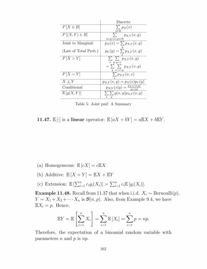
DiscreteP [X ∈ B]
∑x∈B
pX(x)
P [(X, Y ) ∈ R]∑
(x,y):(x,y)∈RpX,Y (x, y)
Joint to Marginal: pX(x) =∑y
pX,Y (x, y)
(Law of Total Prob.) pY (y) =∑x
pX,Y (x, y)
P [X > Y ]∑x
∑y: y<x
pX,Y (x, y)
=∑y
∑x:x>y
pX,Y (x, y)
P [X = Y ]∑x
pX,Y (x, x)
X |= Y pX,Y (x, y) = pX(x)pY (y)
Conditional pX|Y (x|y) =pX,Y (x,y)
pY (y)
E [g(X, Y )]∑x
∑y
g(x, y)pX,Y (x, y)
Table 5: Joint pmf: A Summary
11.47. E [·] is a linear operator: E [aX + bY ] = aEX + bEY .
(a) Homogeneous: E [cX] = cEX
(b) Additive: E [X + Y ] = EX + EY
(c) Extension: E [∑n
i=1 cigi(Xi)] =∑n
i=1 ciE [gi(Xi)].
Example 11.48. Recall from 11.37 that when i.i.d. Xi ∼ Bernoulli(p),Y = X1 +X2 + · · ·Xn is B(n, p). Also, from Example 9.4, we haveEXi = p. Hence,
EY = E
[n∑i=1
Xi
]=
n∑i=1
E [Xi] =n∑i=1
p = np.
Therefore, the expectation of a binomial random variable withparameters n and p is np.
162

Example 11.49. A binary communication link has bit-error prob-ability p. What is the expected number of bit errors in a trans-mission of n bits?
Theorem 11.50 (Expectation and Independence). Two randomvariables X and Y are independent if and only if
E [h(X)g(Y )] = E [h(X)]E [g(Y )]
for all functions h and g.
• In other words, X and Y are independent if and only if forevery pair of functions h and g, the expectation of the producth(X)g(Y ) is equal to the product of the individual expecta-tions.
• One special case is that
X |= Y implies E [XY ] = EX × EY. (32)
However, independence means more than this property. Inother words, having E [XY ] = (EX)(EY ) does not necessarilyimply X |= Y . See Example 11.62.
11.51. Let’s combined what we have just learned about indepen-dence into the definition/equivalent statements that we alreadyhave in 11.32.
The following statements are equivalent:
(a) Random variables X and Y are independent .
(b) [X ∈ B] |= [Y ∈ C] for all B,C.
(c) P [X ∈ B, Y ∈ C] = P [X ∈ B]× P [Y ∈ C] for all B,C.
(d) pX,Y (x, y) = pX(x)× pY (y) for all x, y.
(e) FX,Y (x, y) = FX(x)× FY (y) for all x, y.
(f)
163

Exercise 11.52 (F2011). Suppose X and Y are i.i.d. with EX =EY = 1 and VarX = VarY = 2. Find Var[XY ].
11.53. To quantify the amount of dependence between tworandom variables, we may calculate their mutual information.This quantity is crucial in the study of digital communicationsand information theory. However, in introductory probability class(and introductory communication class), it is traditionally omit-ted.
11.5 Linear Dependence
Definition 11.54. Given two random variables X and Y , we maycalculate the following quantities:
(a) Correlation: E [XY ].
(b) Covariance: Cov [X, Y ] = E [(X − EX)(Y − EY )].
(c) Correlation coefficient: ρX,Y = Cov[X,Y ]σXσY
Exercise 11.55 (F2011). Continue from Exercise 11.9.
(a) Find E [XY ].
(b) Check that Cov [X, Y ] = − 125 .
11.56. Cov [X, Y ] = E [(X − EX)(Y − EY )] = E [XY ]−EXEY
• Note that VarX = Cov [X,X].
11.57. Var [X + Y ] = VarX + VarY + 2Cov [X, Y ]
164

Definition 11.58. X and Y are said to be uncorrelated if andonly if Cov [X, Y ] = 0.
11.59. The following statements are equivalent:
(a) X and Y are uncorrelated.
(b) Cov [X, Y ] = 0.
(c) E [XY ] = EXEY .
(d)
11.60. Independence implies uncorrelatedness; that is if X |= Y ,then Cov [X, Y ] = 0.
The converse is not true. Uncorrelatedness does not imply in-dependence. See Example 11.62.
11.61. The variance of the sum of uncorrelated (or independent)random variables is the sum of their variances.
Example 11.62. Let X be uniform on ±1,±2 and Y = |X|.
165
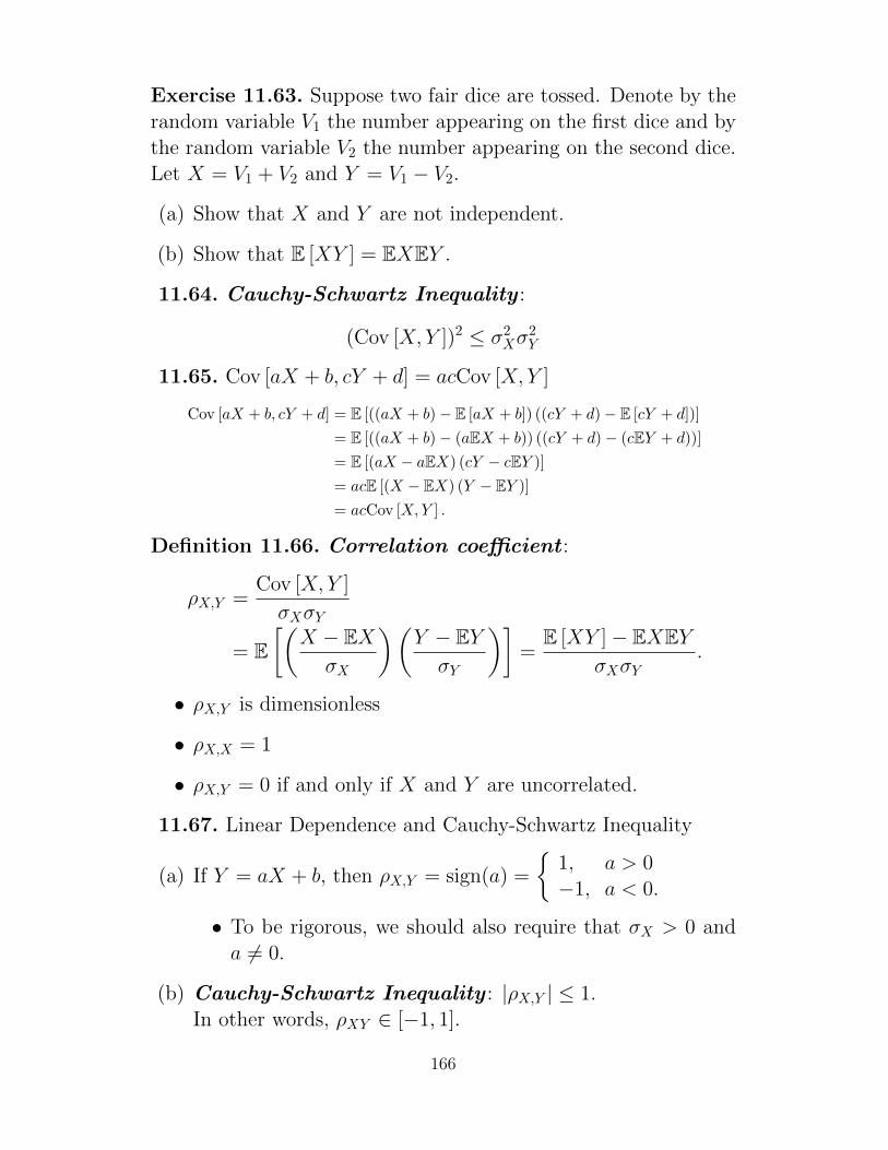
Exercise 11.63. Suppose two fair dice are tossed. Denote by therandom variable V1 the number appearing on the first dice and bythe random variable V2 the number appearing on the second dice.Let X = V1 + V2 and Y = V1 − V2.
(a) Show that X and Y are not independent.
(b) Show that E [XY ] = EXEY .
11.64. Cauchy-Schwartz Inequality :
(Cov [X, Y ])2 ≤ σ2Xσ
2Y
11.65. Cov [aX + b, cY + d] = acCov [X, Y ]
Cov [aX + b, cY + d] = E [((aX + b)− E [aX + b]) ((cY + d)− E [cY + d])]
= E [((aX + b)− (aEX + b)) ((cY + d)− (cEY + d))]
= E [(aX − aEX) (cY − cEY )]
= acE [(X − EX) (Y − EY )]
= acCov [X,Y ] .
Definition 11.66. Correlation coefficient :
ρX,Y =Cov [X, Y ]
σXσY
= E[(
X − EXσX
)(Y − EYσY
)]=
E [XY ]− EXEYσXσY
.
• ρX,Y is dimensionless
• ρX,X = 1
• ρX,Y = 0 if and only if X and Y are uncorrelated.
11.67. Linear Dependence and Cauchy-Schwartz Inequality
(a) If Y = aX + b, then ρX,Y = sign(a) =
1, a > 0−1, a < 0.
• To be rigorous, we should also require that σX > 0 anda 6= 0.
(b) Cauchy-Schwartz Inequality : |ρX,Y | ≤ 1.In other words, ρXY ∈ [−1, 1].
166

(c) When σY , σX > 0, equality occurs if and only if the followingconditions holds
≡ ∃a 6= 0 such that (X − EX) = a(Y − EY )
≡ ∃a 6= 0 and b ∈ R such that X = aY + b
≡ ∃c 6= 0 and d ∈ R such that Y = cX + d
≡ |ρXY | = 1
In which case, |a| = σXσY
and ρXY = a|a| = sgn a. Hence, ρXY
is used to quantify linear dependence between X and Y .The closer |ρXY | to 1, the higher degree of linear dependencebetween X and Y .
Example 11.68. [21, Section 5.2.3] Consider an important factthat investment experience supports: spreading investments overa variety of funds (diversification) diminishes risk. To illustrate,imagine that the random variable X is the return on every investeddollar in a local fund, and random variable Y is the return on everyinvested dollar in a foreign fund. Assume that random variables Xand Y are i.i.d. with expected value 0.15 and standard deviation0.12.
If you invest all of your money, say c, in either the local or theforeign fund, your return R would be cX or cY .
• The expected return is ER = cEX = cEY = 0.15c.
• The standard deviation is cσX = cσY = 0.12c
Now imagine that your money is equally distributed over thetwo funds. Then, the return R is 1
2cX+ 12cY . The expected return
is ER = 12cEX + 1
2cEY = 0.15c. Hence, the expected returnremains at 15%. However,
VarR = Var[c
2(X + Y )
]=c2
4VarX +
c2
4VarY =
c2
2× 0.122.
So, the standard deviation is 0.12√2c ≈ 0.0849c.
In comparison with the distributions of X and Y , the pmf of12(X + Y ) is concentrated more around the expected value. Thecentralization of the distribution as random variables are averagedtogether is a manifestation of the central limit theorem.
167

11.69. [21, Section 5.2.3] Example 11.68 is based on the assump-tion that return rates X and Y are independent from each other.In the world of investment, however, risks are more commonlyreduced by combining negatively correlated funds (two funds arenegatively correlated when one tends to go up as the other falls).
This becomes clear when one considers the following hypothet-ical situation. Suppose that two stock market outcomes ω1 and ω2
are possible, and that each outcome will occur with a probability of12 Assume that domestic and foreign fund returns X and Y are de-termined by X(ω1) = Y (ω2) = 0.25 and X(ω2) = Y (ω1) = −0.10.Each of the two funds then has an expected return of 7.5%, withequal probability for actual returns of 25% and 10%. The randomvariable Z = 1
2(X + Y ) satisfies Z(ω1) = Z(ω2) = 0.075. In otherwords, Z is equal to 0.075 with certainty. This means that an in-vestment that is equally divided between the domestic and foreignfunds has a guaranteed return of 7.5%.
168
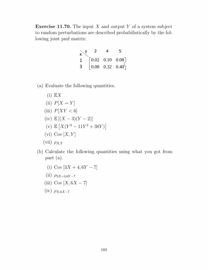
Exercise 11.70. The input X and output Y of a system subjectto random perturbations are described probabilistically by the fol-lowing joint pmf matrix:
0.02 0.10 0.08
0.08 0.32 0.40
y 2 4 5 x 1 3
(a) Evaluate the following quantities.
(i) EX(ii) P [X = Y ]
(iii) P [XY < 6]
(iv) E [(X − 3)(Y − 2)]
(v) E[X(Y 3 − 11Y 2 + 38Y )
](vi) Cov [X, Y ]
(vii) ρX,Y
(b) Calculate the following quantities using what you got frompart (a).
(i) Cov [3X + 4, 6Y − 7]
(ii) ρ3X+4,6Y−7
(iii) Cov [X, 6X − 7]
(iv) ρX,6X−7
169

Answers:
(a)
(i) EX = 2.6
(ii) P [X = Y ] = 0
(iii) P [XY < 6] = 0.2
(iv) E [(X − 3)(Y − 2)] = −0.88
(v) E[X(Y 3 − 11Y 2 + 38Y )
]= 104
(vi) Cov [X, Y ] = 0.032
(vii) ρX,Y = 0.0447
(b)
(i) Hence, Cov [3X + 4, 6Y − 7] = 3× 6× Cov [X, Y ] ≈ 3×6× 0.032 ≈ 0.576 .
(ii) Note that
ρaX+b,cY+d =Cov [aX + b, cY + d]
σaX+bσcY+d
=acCov [X, Y ]
|a|σX |c|σY=
ac
|ac|ρX,Y = sign(ac)× ρX,Y .
Hence, ρ3X+4,6Y−7 = sign(3× 4)ρX,Y = ρX,Y = 0.0447 .
(iii) Cov [X, 6X − 7] = 1 × 6 × Cov [X,X] = 6 × Var[X] ≈3.84 .
(iv) ρX,6X−7 = sign(1× 6)× ρX,X = 1 .
170
Sirindhorn International Institute of Technology
Thammasat University
School of Information, Computer and Communication Technology
ECS315 2013/1 Part V.3 Dr.Prapun
11.6 Pairs of Continuous Random Variables
In this section, we start to look at more than one continuous ran-dom variables. You should find that many of the concepts andformulas are similar if not the same as the ones for pairs of discreterandom variables which we have already studied. For discrete ran-dom variables, we use summations. Here, for continuous randomvariables, we use integrations.
Recall that for a pair of discrete random variables, the jointpmf pX,Y (x, y) completely characterizes the probability model oftwo random variables X and Y . In particular, it does not onlycapture the probability of X and probability of Y individually,it also capture the relationship between them. For continuousrandom variable, we replace the joint pmf by joint pdf.
Definition 11.71. We say that two random variables X and Yare jointly continuous with joint pdf fX,Y (x, y) if48 for anyregion R on the (x, y) plane
P [(X, Y ) ∈ R] =
∫∫(x,y):(x,y)∈R
fX,Y (x, y)dxdy (33)
To understand where Definition 11.71 comes from, it is helpfulto take a careful look at Table 6.
48Remark: If you want to check that a function f(x, y) is the joint pdf of a pair of randomvariables (X,Y ) by using the above definition, you will need to check that (33) is true for anyregion R. This is not an easy task. Hence, we do not usually use this definition for such kindof test. There are some mathematical facts that can be derived from this definition. Suchfacts produce easier condition(s) than (33) but we will not talk about them here.
171

Discrete ContinuousP [X ∈ B]
∑x∈B
pX(x)∫B
fX(x)dx
P [(X, Y ) ∈ R]∑
(x,y):(x,y)∈RpX,Y (x, y)
∫∫(x,y):(x,y)∈R
fX,Y (x, y)dxdy
Table 6: pmf vs. pdf
Example 11.72. Indicate (sketch) the region of integration foreach of the following probabilities
(a) P [1 < X < 2, −1 < Y < 1]
(b) P [X + Y < 3]
11.73. For us, Definition 11.71 is useful because if you know thata function f(x, y) is a joint pdf of a pair of random variables, thenyou can calculate countless possibilities of probabilities involvingthese two random variables via (33). (See, e.g. Example 11.76.)However, the actual calculation of probability from (33) can bedifficult if you have non-rectangular region R or if you have acomplicated joint pdf. In other words, the formula itself is straight-forward and simple, but to carry it out may require that you reviewsome multi-variable integration technique from your calculus class.
11.74. Intuition/Approximation: Note also that the jointpdf’s definition extends the interpretation/approximation that wepreviously discussed for one random variable.
Recall that for a single random variable, the pdf is a measure ofprobability per unit length. In particular, if you want to findthe probability that the value of a random variable X falls insidesome small interval, say the interval [1.5, 1.6], then this probabilitycan be approximated by
P [1.5 ≤ X ≤ 1.6] ≈ fX(1.5)× 0.1.
172
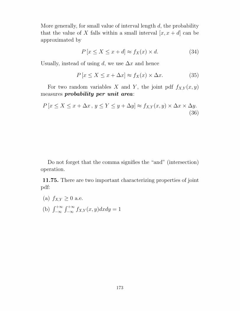
More generally, for small value of interval length d, the probabilitythat the value of X falls within a small interval [x, x + d] can beapproximated by
P [x ≤ X ≤ x+ d] ≈ fX(x)× d. (34)
Usually, instead of using d, we use ∆x and hence
P [x ≤ X ≤ x+ ∆x] ≈ fX(x)×∆x. (35)
For two random variables X and Y , the joint pdf fX,Y (x, y)measures probability per unit area :
P [x ≤ X ≤ x+ ∆x , y ≤ Y ≤ y + ∆y] ≈ fX,Y (x, y)×∆x×∆y.(36)
Do not forget that the comma signifies the “and” (intersection)operation.
11.75. There are two important characterizing properties of jointpdf:
(a) fX,Y ≥ 0 a.e.
(b)∫ +∞−∞
∫ +∞−∞ fX,Y (x, y)dxdy = 1
173

Example 11.76. Consider a probability model of a pair of randomvariables uniformly distributed over a rectangle in the X-Y plane:
fX,Y (x, y) =
c, 0 ≤ x ≤ 5, 0 ≤ y ≤ 30, otherwise.
(a) Find the constant c.
(b) Evaluate P [2 ≤ X ≤ 3, 1 ≤ Y ≤ 3], and P [Y > X]
11.77. Other important properties and definitions for a pair ofcontinuous random variables are summarized in Table 7 along withtheir “discrete counterparts”.
174

Discrete ContinuousP [(X, Y ) ∈ R]
∑(x,y):(x,y)∈R
pX,Y (x, y)∫∫
(x,y):(x,y)∈RfX,Y (x, y)dxdy
Joint to Marginal: pX(x) =∑y
pX,Y (x, y) fX(x) =+∞∫−∞
fX,Y (x, y)dy
(Law of Total Prob.) pY (y) =∑x
pX,Y (x, y) fY (y) =+∞∫−∞
fX,Y (x, y)dx
P [X > Y ]∑x
∑y: y<x
pX,Y (x, y)+∞∫−∞
x∫−∞
fX,Y (x, y)dydx
=∑y
∑x:x>y
pX,Y (x, y) =+∞∫−∞
∞∫y
fX,Y (x, y)dxdy
P [X = Y ]∑x
pX,Y (x, x) 0
X |= Y pX,Y (x, y) = pX(x)pY (y) fX,Y (x, y) = fX(x)fY (y)
Conditional pX|Y (x|y) =pX,Y (x,y)
pY (y)fX|Y (x|y) =
fX,Y (x,y)
fY (y)
Table 7: Important formulas for a pair of discrete RVs and a pair of ContinuousRVs
Exercise 11.78 (F2011). Random variables X and Y have jointpdf
fX,Y (x, y) =
c, 0 ≤ y ≤ x ≤ 1,0, otherwise.
(a) Check that c = 2.
(b) In Figure 25, specify the region of nonzero pdf.
𝑦
x 1
1
Figure 25: Figure for Exercise 11.78b.
(c) Find the marginal density fX(x).
(d) Check that EX = 23 .
175

(e) Find the marginal density fY (y).
(f) Find EY
Definition 11.79. The joint cumulative distribution func-tion (joint cdf ) of random variables X and Y (of any type(s))is defined as
FX,Y (x, y) = P [X ≤ x, Y ≤ y] .
• Although its definition is simple, we rarely use the joint cdfto study probability models. It is easier to work with a prob-ability mass function when the random variables are discrete,or a probability density function if they are continuous.
11.80. The joint cdf for a pair of random variables (of any type(s))has the following properties49.:
(a) 0 ≤ FX,Y (x, y) ≤ 1
(i) FX,Y (∞,∞) = 1.
(ii) FX,Y (−∞, y) = FX,Y (x,−∞) = 0.
(b) Joint to Marginal: FX(x) = FX,Y (x,∞) and FY (y) = FX,Y (∞, y).In words, we obtain the marginal cdf FX and FY directly fromFX,Y by setting the unwanted variable to ∞.
(c) If x1 ≤ x2 and y1 ≤ y2, then FX,Y (x1, y1) ≤ FX,Y (x2, y2)
11.81. The joint cdf for a pair of continuous random variablesalso has the following properties:
(a) FX,Y (x, y) =∫ x−∞∫ y−∞ fX,Y (u, v)dvdu.
(b) fX,Y (x, y) = ∂2
∂x∂yFX,Y (x, y).
49Note that when we write FX,Y (x,∞), we mean limy→∞
FX,Y (x, y). Similar limiting definition
applies to FX,Y (∞,∞), FX,Y (−∞, y), FX,Y (x,−∞), and FX,Y (∞, y)
176

11.82. Independence :The following statements are equivalent:
(a) Random variables X and Y are independent .
(b) [X ∈ B] |= [Y ∈ C] for all B,C.
(c) P [X ∈ B, Y ∈ C] = P [X ∈ B]× P [Y ∈ C] for all B,C.
(d) fX,Y (x, y) = fX(x)× fY (y) for all x, y.
(e) FX,Y (x, y) = FX(x)× FY (y) for all x, y.
Exercise 11.83 (F2011). Let X1 and X2 be i.i.d. E(1)
(a) Find P [X1 = X2].
(b) Find P[X2
1 +X22 = 13
].
11.7 Function of a Pair of Continuous Random Vari-ables: MISO
There are many situations in which we observe two random vari-ables and use their values to compute a new random variable.
Example 11.84. Signal in additive noise : When we says that arandom signal X is transmitted over a channel subject to additivenoise N , we mean that at the receiver, the received signal Y willbe X+N . Usually, the noise is assumed to be zero-mean Gaussiannoise; that is N ∼ N (0, σ2
N) for some noise power σ2N .
Example 11.85. In a wireless channel, the transmitted signalX is corrupted by fading (multiplicative noise). More specifically,the received signal Y at the receiver’s antenna is Y = H ×X.
Remark : In the actual situation, the signal is further corruptedby additive noise N and hence Y = HX + N . However, thisexpression for Y involves more than two random variables andhence we we will not consider it here.
177
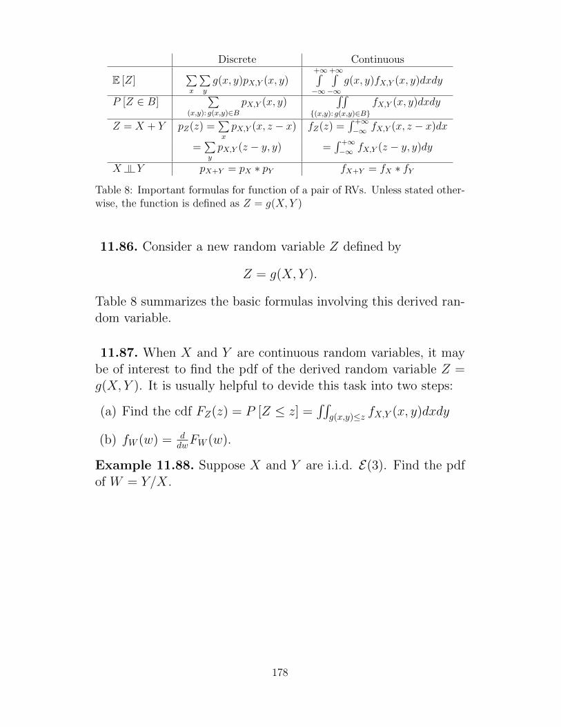
Discrete Continuous
E [Z]∑x
∑y
g(x, y)pX,Y (x, y)+∞∫−∞
+∞∫−∞
g(x, y)fX,Y (x, y)dxdy
P [Z ∈ B]∑
(x,y): g(x,y)∈BpX,Y (x, y)
∫∫(x,y): g(x,y)∈B
fX,Y (x, y)dxdy
Z = X + Y pZ(z) =∑x
pX,Y (x, z − x) fZ(z) =∫ +∞−∞ fX,Y (x, z − x)dx
=∑y
pX,Y (z − y, y) =∫ +∞−∞ fX,Y (z − y, y)dy
X |= Y pX+Y = pX ∗ pY fX+Y = fX ∗ fYTable 8: Important formulas for function of a pair of RVs. Unless stated other-wise, the function is defined as Z = g(X, Y )
11.86. Consider a new random variable Z defined by
Z = g(X, Y ).
Table 8 summarizes the basic formulas involving this derived ran-dom variable.
11.87. When X and Y are continuous random variables, it maybe of interest to find the pdf of the derived random variable Z =g(X, Y ). It is usually helpful to devide this task into two steps:
(a) Find the cdf FZ(z) = P [Z ≤ z] =∫∫
g(x,y)≤z fX,Y (x, y)dxdy
(b) fW (w) = ddwFW (w).
Example 11.88. Suppose X and Y are i.i.d. E(3). Find the pdfof W = Y/X.
178

Exercise 11.89. Let X and Y be i.i.d. N (0, σ2). Show that thepdf of R =
√X2 + Y 2 is given by
fR(r) =
1σ2re
− 12σ2 r
2
, r > 0,0, otherwise.
(37)
Exercise 11.90 (F2011). Let X1 and X2 be i.i.d. E(1).
(a) Define Y = min X1, X2. (For example, when X1 = 6 andX2 = 4, we have Y = 4.) Describe the random variable Y .Does it belong to any known family of random variables? Ifso, what is/are its parameters?
Hint: Y ≥ y if and only if X1 ≥ y and X2 ≥ y.
(b) Define Y = min X1, X2 and Z = max X1, X2. FindfY,Z(2, 1).
(c) Define Y = min X1, X2 and Z = max X1, X2. FindfY,Z(1, 2).
11.91. Observe that finding the pdf of Z = g(X, Y ) is a time-consuming task. If you goal is to find E [Z] do not forget that itcan be calculated directly from
E [g(X, Y )] =
∫ ∫g(x, y)fX,Y (x, y)dxdy.
11.92. The following property is valid for any kind of randomvariables:
E
[∑i
Zi
]=∑i
E [Zi] .
Furthermore,
E
[∑i
gi(X, Y )
]=∑i
E [gi(X, Y )] .
179

Discrete ContinuousP [X ∈ B]
∑x∈B
pX(x)∫B
fX(x)dx
P [(X, Y ) ∈ R]∑
(x,y):(x,y)∈RpX,Y (x, y)
∫∫(x,y):(x,y)∈R
fX,Y (x, y)dxdy
Joint to Marginal: pX(x) =∑y
pX,Y (x, y) fX(x) =+∞∫−∞
fX,Y (x, y)dy
(Law of Total Prob.) pY (y) =∑x
pX,Y (x, y) fY (y) =+∞∫−∞
fX,Y (x, y)dx
P [X > Y ]∑x
∑y: y<x
pX,Y (x, y)+∞∫−∞
x∫−∞
fX,Y (x, y)dydx
=∑y
∑x:x>y
pX,Y (x, y) =+∞∫−∞
∞∫y
fX,Y (x, y)dxdy
P [X = Y ]∑x
pX,Y (x, x) 0
X |= Y pX,Y (x, y) = pX(x)pY (y) fX,Y (x, y) = fX(x)fY (y)
Conditional pX|Y (x|y) =pX,Y (x,y)
pY (y)fX|Y (x|y) =
fX,Y (x,y)
fY (y)
E [g(X, Y )]∑x
∑y
g(x, y)pX,Y (x, y)+∞∫−∞
+∞∫−∞
g(x, y)fX,Y (x, y)dxdy
P [g(X, Y ) ∈ B]∑
(x,y): g(x,y)∈BpX,Y (x, y)
∫∫(x,y): g(x,y)∈B
fX,Y (x, y)dxdy
Z = X + Y pZ(z) =∑x
pX,Y (x, z − x) fZ(z) =∫ +∞−∞ fX,Y (x, z − x)dx
=∑y
pX,Y (z − y, y) =∫ +∞−∞ fX,Y (z − y, y)
Table 9: pmf vs. pdf
180

11.93. Independence : At this point, it is useful to summarizewhat we know about independence. The following statements areequivalent:
(a) Random variables X and Y are independent .
(b) [X ∈ B] |= [Y ∈ C] for all B,C.
(c) P [X ∈ B, Y ∈ C] = P [X ∈ B]× P [Y ∈ C] for all B,C.
(d) For discrete RVs, pX,Y (x, y) = pX(x)× pY (y) for all x, y.For continuous RVs, fX,Y (x, y) = fX(x)× fY (y) for all x, y.
(e) FX,Y (x, y) = FX(x)× FY (y) for all x, y.
(f) E [h(X)g(Y )] = E [h(X)]E [g(Y )] for all functions h and g.
Definition 11.94. All of the definitions involving expectation ofa function of two random variables are the same as in the discretecase:
• Correlation between X and Y : E [XY ].
• Covariance between X and Y :
Cov [X, Y ] = E [(X − EX)(Y − EY )] = E [XY ]− EXEY.
• VarX = Cov [X,X].
• X and Y are said to be uncorrelated if and only if Cov [X, Y ] =0.
• X and Y are said to be orthogonal if E [XY ] = 0.
• Correlation coefficient : ρXY = Cov[X,Y ]σXσY
181
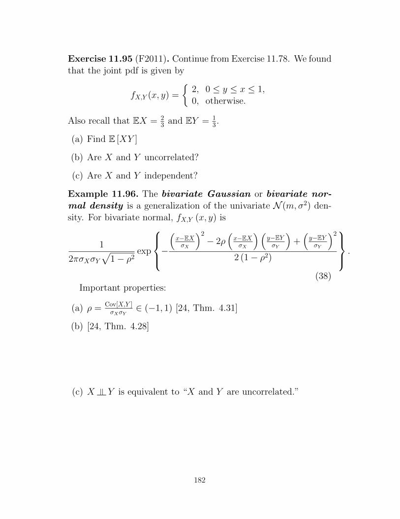
Exercise 11.95 (F2011). Continue from Exercise 11.78. We foundthat the joint pdf is given by
fX,Y (x, y) =
2, 0 ≤ y ≤ x ≤ 1,0, otherwise.
Also recall that EX = 23 and EY = 1
3 .
(a) Find E [XY ]
(b) Are X and Y uncorrelated?
(c) Are X and Y independent?
Example 11.96. The bivariate Gaussian or bivariate nor-mal density is a generalization of the univariate N (m,σ2) den-sity. For bivariate normal, fX,Y (x, y) is
1
2πσXσY√
1− ρ2exp
−(x−EXσX
)2
− 2ρ(x−EXσX
)(y−EYσY
)+(y−EYσY
)2
2 (1− ρ2)
.
(38)Important properties:
(a) ρ = Cov[X,Y ]σXσY
∈ (−1, 1) [24, Thm. 4.31]
(b) [24, Thm. 4.28]
(c) X |= Y is equivalent to “X and Y are uncorrelated.”
182

−5 0 5−6
−4
−2
0
2
4
6
x
y
σX = 1, σY = 1, ρ = 0
−5 0 5−6
−4
−2
0
2
4
6
x
y
σX = 1, σY = 2, ρ = 0
−5 0 5−6
−4
−2
0
2
4
6
x
y
σX = 3, σY = 1, ρ = 0
−5 0 5−6
−4
−2
0
2
4
6
x
y
σX = 1, σY = 2, ρ = 0.5
−5 0 5−6
−4
−2
0
2
4
6
x
yσX = 1, σY = 2, ρ = 0.8
−5 0 5−6
−4
−2
0
2
4
6
x
y
σX = 1, σY = 2, ρ = 0.99
Figure 26: Samples from bivariate Gaussian distributions.
Correlation coefficient
8
Remark: marginal pdfs for both X and Y are standard Gaussian
-2 0 2-3
-2
-1
0
1
2
3
x
y
Number of samples = 2000
-20
2
-2
0
2
0
0.05
0.1
0.15
0.2
xy
Join
t pdf
-2 0 2-3
-2
-1
0
1
2
3
x
y
Number of samples = 2000
-20
2
-2
0
2
0
0.1
0.2
xy
Join
t pdf
-2 0 2-3
-2
-1
0
1
2
3
x
y
Number of samples = 2000
-20
2-2
0
2
0
0.1
0.2
0.3
y
x
Join
t pdf
-2 0 2-3
-2
-1
0
1
2
3
x
y
Number of samples = 2000
-20
2-2
0
2
0
0.05
0.1
0.15
0.2
y
x
Join
t pdf
Figure 27: Effect of ρ on bivariate Gaussian distribution. Note that the marginalpdfs for both X and Y are all standard Gaussian.
183

Sirindhorn International Institute of Technology
Thammasat University
School of Information, Computer and Communication Technology
ECS315 2013/1 Part VI Dr.Prapun
12 Three Types of Random Variables
12.1. Review: You may recall50 the following properties for cdfof discrete random variables. These properties hold for any kindof random variables.
(a) The cdf is defined as FX(x) = P [X ≤ x]. This is valid forany type of random variables.
(b) Moreover, the cdf for any kind of random variable must sat-isfies three properties which we have discussed earlier:
CDF1 FX is non-decreasing
CDF2 FX is right-continuous
CDF3 limx→−∞
FX (x) = 0 and limx→∞
FX (x) = 1.
(c) P [X = x] = FX (x) − FX (x−) = the jump or saltus in F atx.
Theorem 12.2. If you find a function F that satisfies CDF1,CDF2, and CDF3 above, then F is a cdf of some random variable.
50If you don’t know these properties by now, you should review them as soon as possible.
184

Example 12.3. Consider an input X to a device whose output Ywill be the same as the input if the input level does not exceed 5.For input level that exceeds 5, the output will be saturated at 5.Suppose X ∼ U(0, 6). Find FY (y).
12.4. We can categorize random variables into three types ac-cording to its cdf:
(a) If FX(x) is piecewise flat with discontinuous jumps, then X
is discrete.
(b) If FX(x) is a continuous function, then X is continuous.
(c) If FX(x) is a piecewise continuous function with discontinu-ities, then X is mixed.
185

81 3.1 Random variables1.0
1.0
1.0
0–¥ ¥
–¥ ¥
–¥ ¥
x
x
x
0
0
Fx(x)
Fx(x)
Fx(x)
(a)
(b)
(c)
Fig. 3.2Typical cdfs: (a) a discrete random variable, (b) a continuous random variable, and (c) a mixed randomvariable.
For a discrete random variable, Fx(x) is a staircase function, whereas a random variableis called continuous if Fx(x) is a continuous function. A random variable is called mixedif it is neither discrete nor continuous. Typical cdfs for discrete, continuous, and mixedrandom variables are shown in Figures 3.2(a), 3.2(b), and 3.2(c), respectively.
Rather than dealing with the cdf, it is more common to deal with the probability densityfunction (pdf), which is defined as the derivative of Fx(x), i.e.,
fx(x) = dFx(x)
dx. (3.11)
From the definition it follows that
P(x1 ≤ x ≤ x2) = P(x ≤ x2)− P(x ≤ x1)
= Fx(x2)− Fx(x1)
=∫ x2
x1
fx(x)dx. (3.12)
Figure 28: Typical cdfs: (a) a discrete random variable, (b) a continuous randomvariable, and (c) a mixed random variable [16, Fig. 3.2].
186

We have seen in Example 12.3 that some function can turn acontinuous random variable into a mixed random variable. Next,we will work on an example where a continuous random variableis turned into a discrete random variable.
Example 12.5. Let X ∼ U(0, 1) and Y = g(X) where
g(x) =
1, x < 0.60, x ≥ 0.6.
Before going deeply into the math, it is helpful to think about thenature of the derived random variable Y . The definition of g(x)tells us that Y has only two possible values, Y = 0 and Y = 1.Thus, Y is a discrete random variable.
Example 12.6. In MATLAB, we have the rand command to gen-erate U(0, 1). If we want to generate a Bernoulli random variablewith success probability p, what can we do?
Exercise 12.7. In MATLAB, how can we generateX ∼ binomial(2, 1/4)from the rand command?
187

13 Transform methods: Characteristic Func-
tions
Definition 13.1. The characteristic function of a random variableX is defined by
ϕX(v) = E[ejvX
].
Remarks:
(a) If X is a continuous random variable with density fX , then
ϕX(v) =
∫ +∞
−∞ejvxfX(x)dx,
which is the Fourier transform of fX evaluated at −v. Moreprecisely,
ϕX(v) = F fX (ω)|ω=−v . (39)
(b) Many references use u or t instead of v.
Example 13.2. You may have learned that the Fourier transformof a Gaussian waveform is a Gaussian waveform. In fact, whenX ∼ N (m,σ2),
F fX (ω) =
∞∫−∞
fX (x) e−jωxdx = e−jωm−12ω
2σ2
.
Using (39), we have
ϕX(v) = ejvm−12v
2σ2
.
Example 13.3. For X ∼ E(λ), we have ϕX(v) = λλ−jv .
188

As with the Fourier transform, we can build a large list of com-monly used characteristic functions. (You probably remember thatrectangular function in time domain gives a sinc function in fre-quency domain.) When you see a random variable that has thesame form of characteristic function as the one that you know, youcan quickly make a conclusion about the family and parameters ofthat random variable.
Example 13.4. Suppose a random variable X has the character-istic function ϕX(v) = 2
2−jv . You can quickly conclude that it isan exponential random variable with parameter 2.
For many random variables, it is easy to find its expected valueor any moments via the characteristic function. This can be donevia the following result.
13.5. ϕ(k)X (v) = jkE
[XkejvX
]and ϕ
(k)X (0) = jkE
[Xk].
Example 13.6. When X ∼ E(λ),
(a) EX = 1λ .
(b) VarX = 1λ2 .
189

Exercise 13.7 (F2011). Continue from Example 13.2.
(a) Show that for X ∼ N (m,σ2), we have
(i) EX = m
(ii) E[X2]
= σ2 +m2.
(b) for X ∼ N (3, 4), find E[X3].
One very important properties of characteristic function is thatit is very easy to find the characteristic function of a sum of inde-pendent random variables.
13.8. Suppose X |= Y . Let Z = X + Y . Then, the characteristicfunction of Z is the product of the characteristic functions of Xand Y :
ϕZ(v) = ϕX(v)ϕY (v)
Remark: Can you relate this property to the property of theFourier transform?
Example 13.9. Use 13.8 to show that the sum of two independentGaussian random variables is still a Gaussian random variable:
Exercise 13.10. Continue from Example 11.44. Suppose Λ1 ∼P(λ1) and Λ2 ∼ P(λ2) are independent. Let Λ = Λ1 + Λ2. Use13.8 to show that Λ ∼ P(λ1 + λ2).
Exercise 13.11. Continue from Example 11.45 Suppose B1 ∼B(n1, p) and B2 ∼ B(n2, p) are independent. Let B = B1 + B2.Use 13.8 to show that B ∼ B(n1 + n2, p).
190
Sirindhorn International Institute of Technology
Thammasat University
School of Information, Computer and Communication Technology
ECS315 2013/1 Part VII Dr.Prapun
14 Limiting Theorems
14.1 Law of Large Numbers (LLN)
Definition 14.1. Let X1, X2, . . . , Xn be a collection of randomvariables with a common mean E [Xi] = m for all i. In practice,since we do not know m, we use the numerical average, or samplemean,
Mn =1
n
n∑i=1
Xi
in place of the true, but unknown value, m.
Q: Can this procedure of using Mn as an estimate of m bejustified in some sense?
A: This can be done via the law of large number.
14.2. The law of large number basically says that if you have asequence of i.i.d random variables X1, X2, . . .. Then the samplemeans Mn = 1
n
∑ni=1Xi will converge to the actual mean as n →
∞.
14.3. LLN is easy to see via the property of variance. Note that
E [Mn] = E
[1
n
n∑i=1
Xi
]=
1
n
n∑i=1
EXi = m
and
Var[Mn] = Var
[1
n
n∑i=1
Xi
]=
1
n2
n∑i=1
VarXi =1
nσ2, (40)
191

Remarks:
(a) For (40) to hold, it is sufficient to have uncorrelated Xi’s.
(b) From (40), we also have
σMn=
1√nσ. (41)
In words, “when uncorrelated (or independent) random vari-ables each having the same distribution are averaged together,the standard deviation is reduced according to the square rootlaw.” [21, p 142].
Exercise 14.4 (F2011). Consider i.i.d. random variablesX1, X2, . . . , X10.Define the sample mean M by
M =1
10
10∑k=1
Xk.
Let
V1 =1
10
10∑k=1
(Xk − E [Xk])2.
and
V2 =1
10
10∑j=1
(Xj −M)2.
Suppose E [Xk] = 1 and Var[Xk] = 2.
(a) Find E [M ].
(b) Find Var[M ].
(c) Find E [V1].
(d) Find E [V2].
192
14.2 Central Limit Theorem (CLT)
In practice, there are many random variables that arise as a sumof many other random variables. In this section, we consider thesum
Sn =n∑i=1
Xi (42)
where theXi are i.i.d. with common meanm and common varianceσ2.
• Note that when we talk about Xi being i.i.d., the definitionis that they are independent and identically distributed. Itis then convenient to talk about a random variable X whichshares the same distribution (pdf/pmf) with these Xi. Thisallow us to write
Xii.i.d.∼ X, (43)
which is much more compact than saying that the Xi arei.i.d. with the same distribution (pdf/pmf) as X. Moreover,we can also use EX and σ2
X for the common expected valueand variance of the Xi.
Q: How does Sn behave?
For the Sn defined above, there are many cases for which weknow the pmf/pdf of Sn.
Example 14.5. When the Xi are i.i.d. Bernoulli(p),
Example 14.6. When the Xi are i.i.d. N (m,σ2),
Note that it is not difficult to find the characteristic functionof Sn if we know the common characteristic function ϕX(v) of the
193

Xi:ϕSn(v) = (ϕX(v))n .
If we are lucky, as in the case for the sum of Gaussian random vari-ables in Example 14.6 above, we get ϕSn(v) that is of the form thatwe know. However, ϕSn(v) will usually be something we haven’tseen before or difficult to find the inverse transform. This is oneof the reason why having a way to approximate the sum Sn wouldbe very useful.
There are also some situations where the distribution of the Xi
is unknown or difficult to find. In which case, it would be amazingif we can say something about the distribution of Sn.
In the previous section, we consider the sample mean of identi-cally distributed random variables. More specifically, we considerthe random variable Mn = 1
nSn. We found that Mn will convergeto m as n increases to ∞. Here, we don’t want to rescale the sumSn by the factor 1
n .
14.7 (Approximation of densities and pmfs using the CLT). Theactual statement of the CLT is a bit difficult to state. So, we firstgive you the interpretation/insight from CLT which is very easyto remember and use:
For n large enough, we can approximate Sn by a Gaus-sian random variable with the same mean and variance asSn.
Note that the mean and variance of Sn is nm and nσ2, re-spectively. Hence, for n large enough we can approximate Sn byN(nm, nσ2
). In particular,
(a) FSn(s) ≈ Φ(s−nmσ√n
).
(b) If the Xi are continuous random variable, then
fSn(s) ≈1√
2πσ√ne−
12(
x−nmσ√n )
2
.
(c) If the Xi are integer-valued, then
P [Sn = k] = P
[k − 1
2< Sn ≤ k +
1
2
]≈ 1√
2πσ√ne−
12(
k−nmσ√n )
2
.
194

[9, eq (5.14), p. 213].
The approximation is best for k near nm [9, p. 211].
Example 14.8. Approximation for Binomial Distribution: ForX ∼ B(n, p), when n is large, binomial distribution becomes diffi-cult to compute directly because of the need to calculate factorialterms.
(a) When p is not close to either 0 or 1 so that the variance isalso large, we can use CLT to approxmiate
P [X = k] ≈ 1√2πVarX
e−(k−EX)2
2 VarX (44)
=1√
2πnp (1− p)e−
(k−np)22np(1−p) . (45)
This is called Laplace approximation to the Binomial distri-bution [25, p. 282].
(b) When p is small, the binomial distribution can be approxi-mated by P(np) as discussed in 8.45.
(c) If p is very close to 1, then n−X will behave approximatelyPoisson.
• Normal Approximation to Poisson Distribution with large λ:
Let ( )~X λP . X can be though of as a sum of i.i.d. ( )0~iX λP , i.e., 1
n
ii
X X=
= ∑ , where
0nλ λ= . Hence X is approximately normal ( ),λ λN for λ large.
Some says that the normal approximation is good when 5λ > .
The above figure compare 1) Poisson when x is integer, 2) Gaussian, 3) Gamma, 4) Binomial.
• If :g + →Z R is any bounded function and ( )~ λΛ P , then ( ) ( )1 0g gλ Λ + − Λ Λ =⎡ ⎤⎣ ⎦E .
Proof. ( ) ( )( ) ( ) ( )
( ) ( )
1
0 0 1
1 1
0 0
1 1! ! !
1 1! !
0
i i i
i i i
i m
i m
g i ig i e e g i ig ii i i
e g i g mi m
λ λ
λ
λ λ λλ
λ λ
+∞ ∞ ∞− −
= = =
+ +∞ ∞−
= =
⎛ ⎞+ − = + −⎜ ⎟
⎝ ⎠⎛ ⎞
= + − +⎜ ⎟⎝ ⎠
=
∑ ∑ ∑
∑ ∑
Any function :f + →Z R for which ( ) 0f Λ =⎡ ⎤⎣ ⎦E can be expressed in the form
( ) ( ) ( )1f j g j jg jλ= + − for a bounded function g.
Thus, conversely, if ( ) ( )1 0g gλ Λ + − Λ Λ =⎡ ⎤⎣ ⎦E for all bounded g, then Λ has the Poisson
distribution ( )λP .
• Poisson distribution can be obtained as a limit from negative binomial distributions. (Thus, the negative binomial distribution with parameters r and p can be approximated by the
Poisson distribution with parameter rqp
λ = (maen-matching), provided that p is
“sufficiently” close to 1 and r is “sufficiently” large. • Let X be Poisson with mean λ . Suppose, that the mean λ is chosen in accord with a
probability distribution ( )F λΛ . Hence,
p 0.05:= n 100:= λ 5:=
0 5 100
0.05
0.1
0.15e λ− λx
Γ x 1+( )⋅
1
2 π⋅ λe
1−2 λ⋅
x λ−( )2
⋅
e x− xλ 1−⋅
Γ λ( )
Γ n 1+( )
Γ n x− 1+( ) Γ x 1+( )⋅px⋅ 1 p−( ) n x−⋅
x
p 0.05:= n 800:= λ 40:=
0 20 40 600
0.02
0.04
0.06e λ− λx
Γ x 1+( )⋅
1
2 π⋅ λe
1−2 λ⋅
x λ−( )2
⋅
e x− xλ 1−⋅
Γ λ( )
Γ n 1+( )
Γ n x− 1+( ) Γ x 1+( )⋅px⋅ 1 p−( ) n x−⋅
x
Figure 29: Gaussian approximation to Binomial, Poisson distribution, andGamma distribution.
195

Exercise 14.9 (F2011). Continue from Exercise 6.53. The strongerperson (Kakashi) should win the competition if n is very large. (Bythe law of large numbers, the proportion of fights that Kakashi winsshould be close to 55%.) However, because the results are randomand n can not be very large, we can not guarantee that Kakashiwill win. However, it may be good enough if the probability thatKakashi wins the competition is greater than 0.85.
We want to find the minimal value of n such that the probabilitythat Kakashi wins the competition is greater than 0.85.
Let N be the number of fights that Kakashi wins among the nfights. Then, we need
P[N >
n
2
]≥ 0.85. (46)
Use the central limit theorem and Table 3.1 or Table 3.2 from[Yates and Goodman] to approximate the minimal value of n suchthat (46) is satisfied.
14.10. A more precise statement for CLT can be expressed via theconvergence of the characteristic function. In particular, supposethat (Xk)k≥1 is a sequence of i.i.d. random variables with mean mand variance 0 < σ2 < ∞. Let Sn =
∑nk=1Xk. It can be shown
that
(a) the characteristic function of Sn−mnσ√n
converges pointwise to
the characteristic function of N (0, 1) and that
(b) the characteristic function of Sn−mn√n
converges pointwise to
the characteristic function of N (0, σ).
To see this, let Zk = Xk−mσ
iid∼Z and Yn = 1√n
∑nk=1 Zk. Then,
EZ = 0, VarZ = 1, and ϕYn(t) =(ϕZ( t√
n))n
. By approximating
ex ≈ 1 + x+ 12x
2. We have ϕX (t) ≈ 1 + jtEX − 12t
2E[X2]
and
ϕYn(t) =
(1− 1
2
t2
n
)n→ e−
t2
2 ,
which is the characteristic function of N (0, 1).
196

• The case of Bernoulli(1/2) was derived by Abraham de Moivrearound 1733. The case of Bernoulli(p) for 0 < p < 1 wasconsidered by Pierre-Simon Laplace [9, p. 208].
197

15 Random Vector
In Section 11.2, we have introduced the way to deal with more thantwo random variables. In particular, we introduce the concepts ofjoint pmf:
pX1,X2,...,Xn(x1, x2, . . . , xn) = P [X1 = x1, X2 = x2, . . . , Xn = xn]
and joint pdf:fX1,X2,...,Xn
(x1, x2, . . . , xn)
of a collection of random variables.
Definition 15.1. You may notice that it is tedious to write then-tuple (X1, X2, . . . , Xn) every time that we want to refer to thiscollection of random variables. A more convenient notation usesa column vector X to represent all of them at once, keeping inmind that the ith component of X is the random variable Xi. Thisallows us to express
(a) pX1,X2,...,Xn(x1, x2, . . . , xn) as pX(x) and
(b) fX1,X2,...,Xn(x1, x2, . . . , xn) as fX(x).
When the random variables are separated into two groups, we maylabel those in a group as X1, X2, . . . , Xn and those in another groupas Y1, Y2, . . . , Ym. In which case, we can express
(a) pX1,...,Xn,Y1,...,Ym(x1, . . . , xn, y1, . . . , ym) as pX,Y(x,y) and
(b) fX1,...,Xn,Y1,...,Ym(x1, . . . , xn, y1, . . . , ym) as fX,Y(x,y).
Definition 15.2. Random vectors X and Y are independent ifand only if
(a) Discrete: pX,Y(x,y) = pX(x)pY(y).
(b) Continuous: fX,Y(x,y) = fX(x)fY(y).
Definition 15.3. A random vector X contains many random vari-ables. Each of these random variables has its own expected value.We can represent the expected values of all these random variablesin the form of a vector as well by using the notation E [X]. Thisis a vector whose ith component is EXi.
198

• In other words, the expectation E [X] of a random vector Xis defined to be the vector of expectations of its entries.
• E [X] is usually denoted by µX or mX.
Definition 15.4. Recall that a random vector is simply a vectorcontaining random variables as its components. We can also talkabout random matrix which is simply a matrix whose entriesare random variables. In which case, we define the expectation ofa random matrix to be a matrix whose entries are expectation ofthe corresponding random variables in the random matrix.
Example 15.5.
E[(
X
Y
)]=
(EXEY
)and
E[(
X WY Z
)]=
(EX EWEY EZ
)15.6. For non-random matrix A,B,C and a random vector X,
E [AXB + C] = A (EX)B + C.
Correlation and covariance are important quantities that cap-ture linear dependency between two random variables. When wehave many random variables, there are many possible pairs to findcorrelation E [XiXj] and covariance Cov [Xi, Xj]. All of the corre-lation values can be expressed at once using the correlation matrix.
Definition 15.7. The correlation matrix RX of a random (col-umn) vector X is defined by
RX = E[XXT
].
Note that it is symmetric and that the ij-entry of RX is simplyE [XiXj].
Example 15.8. Consider X =
(X1
X2
).
RX = E[XXT
]= E
[(X1
X2
)(X1 X2
)]= E
[(X2
1 X1X2
X1X2 X22
)]=
(E[X2
1
]E [X1X2]
E [X1X2] E[X2
2
] )199
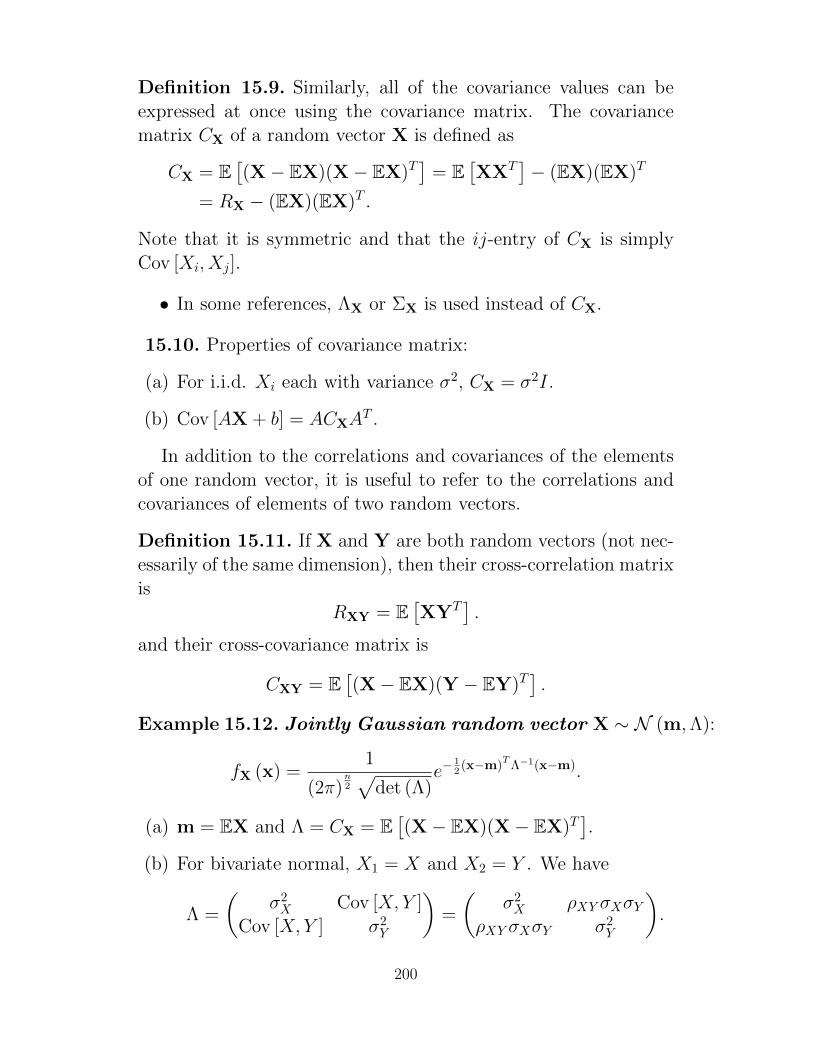
Definition 15.9. Similarly, all of the covariance values can beexpressed at once using the covariance matrix. The covariancematrix CX of a random vector X is defined as
CX = E[(X− EX)(X− EX)T
]= E
[XXT
]− (EX)(EX)T
= RX − (EX)(EX)T .
Note that it is symmetric and that the ij-entry of CX is simplyCov [Xi, Xj].
• In some references, ΛX or ΣX is used instead of CX.
15.10. Properties of covariance matrix:
(a) For i.i.d. Xi each with variance σ2, CX = σ2I.
(b) Cov [AX + b] = ACXAT .
In addition to the correlations and covariances of the elementsof one random vector, it is useful to refer to the correlations andcovariances of elements of two random vectors.
Definition 15.11. If X and Y are both random vectors (not nec-essarily of the same dimension), then their cross-correlation matrixis
RXY = E[XYT
].
and their cross-covariance matrix is
CXY = E[(X− EX)(Y − EY)T
].
Example 15.12. Jointly Gaussian random vector X ∼ N (m,Λ):
fX (x) =1
(2π)n2
√det (Λ)
e−12 (x−m)
TΛ−1(x−m).
(a) m = EX and Λ = CX = E[(X− EX)(X− EX)T
].
(b) For bivariate normal, X1 = X and X2 = Y . We have
Λ =
(σ2X Cov [X, Y ]
Cov [X, Y ] σ2Y
)=
(σ2X ρXY σXσY
ρXY σXσY σ2Y
).
200

16 Introduction to Stochastic Processes (Ran-
dom Processes)
A random process consider an infinite collection of random vari-ables. These random variables are usually indexed by time. So,the obvious notation for random process would be X(t). As inthe signals-and-systems class, time can be discrete or continu-ous. When time is discrete, it may be more appropriate to useX1, X2, . . . or X[1], X[2], X[3], . . . to denote a random process.
Example 16.1. Sequence of results (0 or 1) from a sequence ofBernoulli trials is a discrete-time random process.
16.2. Two perspectives:
(a) We can view a random process as a collection of many randomvariables indexed by t.
(b) We can also view a random process as the outcome of a ran-dom experiment, where the outcome of each trial is a deter-ministic waveform (or sequence) that is a function of t.
The collection of these functions is known as an ensemble ,and each member is called a sample function.
Example 16.3. Gaussian Random Processes: A random processX(t) is Gaussian if for all positive integers n and for all t1, t2, . . . , tn,the random variables X(t1), X(t2), . . . , X(tn) are jointly Gaussianrandom variables.
16.4. Formal definition of random process requires going back tothe probability space (Ω,A, P ).
Recall that a random variable X is in fact a deterministic func-tion of the outcome ω from Ω. So, we should have been writingit as X(ω). However, as we get more familiar with the concept ofrandom variable, we usually drop the “(ω)” part and simply referto it as X.
For random process, we have X(t, ω). This two-argument ex-pression corresponds to the two perspectives that we have justdiscussed earlier.
201

(a) When you fix the time t, you get a random variable from arandom process.
(b) When you fix ω, you get a deterministic function of time froma random process.
As we get more familiar with the concept of random processes, weagain drop the ω argument.
Definition 16.5. A sample function x(t, ω) is the time functionassociated with the outcome ω of an experiment.
Example 16.6 (Randomly Scaled Sinusoid). Consider the randomprocess defined by
X(t) = A× cos(1000t)
where A is a random variable. For example, A could be a Bernoullirandom variable with parameter p.
This is a good model for a one-shot digital transmission viaamplitude modulation.
(a) Consider the time t = 2 ms. X(t) is a random variable takingthe value 1 cos(2) = −0.4161 with probability p and value0 cos(2) = 0 with probability 1− p.If you consider t = 4 ms. X(t) is a random variable takingthe value 1 cos(4) = −0.6536 with probability p and value0 cos(4) = 0 with probability 1− p.
(b) From another perspective, we can look at the process X(t) astwo possible waveforms cos(1000t) and 0. The first one hap-pens with probability p; the second one happens with proba-bility 1 − p. In this view, notice that each of the waveformsis not random. They are deterministic. Randomness in thissituation is associated not with the waveform but with theuncertainty as to which waveform will occur in a given trial.
202

92 Probability theory, random variables and random processes
t0
(c)
t
+V
−V
(d)
0
Tb
(a)
0 t
(b)
t0
Fig. 3.8Typical ensemble members for four random processes commonly encountered in communications: (a)thermal noise, (b) uniform phase, (c) Rayleigh fading process, and (d) binary random data process.
x(t) =∞∑
k=−∞V(2ak − 1)[u(t − kTb + ε)− u(t − (k + 1)Tb + ε)], (3.46)
where ak = 1 with probability p, 0 with probability (1− p) (usually p = 1/2), Tb is the bitduration, and ε is uniform over [0, Tb).
Observe that two of these ensembles have member functions that look very determin-istic, one is “quasi” deterministic but for the last one even individual time functions lookrandom. But the point is not whether any one member function looks deterministic ornot; the issue when dealing with random processes is that we do not know for sure whichmember function we shall have to deal with.
3.2.1 Classification of random processes
The basic classification of random processes arises from whether its statistics change withtime or not, i.e., whether the process is nonstationary or stationary. Even if stationary
Figure 30: Typical ensemble members for four random processes commonlyencountered in communications: (a) thermal noise, (b) uniform phase (encoun-tered in communication systems where it is not feasible to establish timing atthe receiver.), (c) Rayleigh fading process, and (d) binary random data process(which may represent transmitted bits 0 and 1 that are mapped to +V and V(volts)). [16, Fig. 3.8]
203

Definition 16.7. At any particular time t, because we have arandom variable, we can also find its expected value. The functionmX(t) captures these expected values as a deterministic functionof time:
mX(t) = E [X(t)] .
16.1 Autocorrelation Function and WSS
One of the most important characteristics of a random process is itsautocorrelation function, which leads to the spectral information ofthe random process. The frequency content process depends on therapidity of the amplitude change with time. This can be measuredby correlating the values of the process at two time instances tl andt2.
Definition 16.8. Autocorrelation Function : The autocorre-lation function RX(t1, t2) for a random process X(t) is defined by
RX(t1, t2) = E [X(t1)X(t2)] .
Example 16.9. The random process x(t) is a slowly varying pro-cess compared to the process y(t) in Figure 31. For x(t), the valuesat tl and t2 are similar; that is, have stronger correlation. On theother hand, for y(t), values at tl and t2 have little resemblance,that is, have weaker correlation.
Example 16.10 (Randomly Phased Sinusoid). Consider a ran-dom process
X(t) = 5 cos(7t+ Θ)
where Θ is a uniform random variable on the interval (0, 2π).
mX(t) = E [X(t)] =
∫ +∞
−∞5 cos(7t+ θ)fΘ(θ)dθ
=
∫ 2π
0
5 cos(7t+ θ)1
2πdθ = 0.
204

(c)
T_
Figure 31: Autocorrelation functions for a slowly varying and a rapidly varyingrandom process [13, Fig. 11.4]
and
RX(t1, t2) = E [X(t1)X(t2)]
= E [5 cos(7t1 + Θ)× 5 cos(7t2 + Θ)]
=25
2cos (7(t2 − t1)) .
Definition 16.11. A random process whose statistical character-istics do not change with time is classified as a stationary randomprocess. For a stationary process, we can say that a shift of timeorigin will be impossible to detect; the process will appear to bethe same.
Example 16.12. The random process representing the tempera-ture of a city is an example of a nonstationary process, becausethe temperature statistics (mean value, for example) depend onthe time of the day.
On the other hand, the noise process is stationary, because itsstatistics (the mean ad the mean square values, for example) donot change with time.
205

16.13. In general, it is not easy to determine whether a processis stationary. In practice, we can ascertain stationary if there is nochange in the signal-generating mechanism. Such is the case forthe noise process.
A process may not be stationary in the strict sense. A morerelaxed condition for stationary can also be considered.
Definition 16.14. A random process X(t) is wide-sense sta-tionary (WSS) if
(a) mX(t) is a constant
(b) RX(t1, t2) depends only on the time difference t2−t1 and doesnot depend on the specific values of t1 and t2.
In which case, we can write the correlation function as RX(τ)where τ = t2 − t1.• One important consequence is that E
[X2(t)
]will be a con-
stant as well.
Example 16.15. The random process defined in Example 16.9 isWSS with
RX(τ) =25
2cos (7τ) .
16.16. Most information signals and noise sources encounteredin communication systems are well modeled as WSS random pro-cesses.
Example 16.17. White noise process is a WSS process N(t)whose
(a) E [N(t)] = 0 for all t and
(b) RN(τ) = N0
2 δ(τ).
See also 16.23 for its definition.
• Since RN(τ) = 0 for τ 6= 0, any two different samples ofwhite noise, no matter how close in time they are taken, areuncorrelated.
206

Example 16.18. [Thermal noise] A statistical analysis of the ran-dom motion (by thermal agitation) of electrons shows that theautocorrelation of thermal noise N(t) is well modeled as
RN(τ) = kTGe−
τt0
t0watts,
where k is Boltzmann’s constant (k = 1.38 × 10⁻²³ joule/degreeKelvin), G is the conductance of the resistor (mhos), T is the(ambient) temperature in degrees Kelvin, and t0 is the statisticalaverage of time intervals between collisions of free electrons in theresistor, which is on the order of 10−12 seconds. [16, p. 105]
16.2 Power Spectral Density (PSD)
An electrical engineer instinctively thinks of signals and linear sys-tems in terms of their frequency-domain descriptions. Linear sys-tems are characterized by their frequency response (the transferfunction), and signals are expressed in terms of the relative am-plitudes and phases of their frequency components (the Fouriertransform). From the knowledge of the input spectrum and trans-fer function, the response of a linear system to a given signal can beobtained in terms of the frequency content of that signal. This isan important procedure for deterministic signals. We may wonderif similar methods may be found for random processes.
In the study of stochastic processes, the power spectral densityfunction, SX(f), provides a frequency-domain representation of thetime structure of X(t). Intuitively, SX(f) is the expected valueof the squared magnitude of the Fourier transform of a samplefunction of X(t).
You may recall that not all functions of time have Fourier trans-forms. For many functions that extend over infinite time, theFourier transform does not exist. Sample functions x(t) of a sta-tionary stochastic process X(t) are usually of this nature. To workwith these functions in the frequency domain, we begin with XT (t),a truncated version of X(t). It is identical to X(t) for −T ≤ t ≤ Tand 0 elsewhere. We use FXT(f) to represent the Fourier trans-form of XT (t) evaluated at the frequency f .
207

Definition 16.19. Consider a WSS process X(t). The powerspectral density (PSD) is defined as
SX(f) = limt→∞
1
2TE[|FXT(f)|2
]= lim
t→∞1
2TE
[∣∣∣∣∫ T
−TX(t)e−j2πftdt
∣∣∣∣2]
We refer to SX(f) as a density function because it can be in-terpreted as the amount of power in X(t) in the small band offrequencies from f to f + df .
16.20. Wiener-Khinchine theorem : the PSD of a WSS ran-dom process is the Fourier transform of its autocorrelation func-tion:
SX(f) =
∫ +∞
−∞RX(τ)e−j2πfτdτ
and
RX(τ) =
∫ +∞
−∞SX(f)ej2πfτdf.
One important consequence is
RX(0) = E[X2(t)
]=
∫ +∞
−∞SX(f)df.
Example 16.21. For the thermal noise in Example 16.18, thecorresponding PSD is SN(f) = 2kTG
1+(2πft0)2 watts/hertz.
16.22. Observe that the thermal noise’s PSD in Example 16.21is approximately flat over the frequency range 0–10 gigahertz. Asfar as a typical communication system is concerned we might aswell let the spectrum be flat from 0 to ∞, i.e.,
SN(f) =N0
2watts/hertz,
where N0 is a constant; in this case N0 = 4kTG.
208

97 3.2 Random processesx1(t, ω1) |X1( f, ω1)|
|X2( f, ω2)|
|XM( f, ωM)|
x2(t, ω2)
xM(t, ωM)
t
t0
0
0
0
0
0
f
f
f.
.
.
.
.
.
.
.
.
.
.
.
Time-domain ensemble Frequency-domain ensemble
t
Fig. 3.9Fourier transforms of member functions of a random process. For simplicity, only the magnitude spectraare shown.
What we have managed to accomplish thus far is to create the random variable, P, whichin some sense represents the power in the process. Now we find the average value of P, i.e.,
EP = E
1
2T
∫ T
−Tx2
T (t)dt
= E
1
2T
∫ ∞
−∞|XT (f )|2 df
. (3.64)
Figure 32: Fourier transforms of member functions of a random process. Forsimplicity, only the magnitude spectra are shown. [16, Fig. 3.9]
209
Definition 16.23. Noise that has a uniform spectrum over theentire frequency range is referred to as white noise. In particular,for white noise,
SN(f) =N0
2watts/hertz,
• The factor 2 in the denominator is included to indicate thatSN(f) is a two-sided spectrum.
• The adjective “white” comes from white light, which containsequal amounts of all frequencies within the visible band ofelectromagnetic radiation.
• The average power of white noise is obviously infinite.
(a) White noise is therefore an abstraction since no physicalnoise process can truly be white.
(b) Nonetheless, it is a useful abstraction.
The noise encountered in many real systems can beassumed to be approximately white.
This is because we can only observe such noise afterit has passed through a real system, which will havea finite bandwidth. Thus, as long as the bandwidthof the noise is significantly larger than that of thesystem, the noise can be considered to have an infinitebandwidth.
As a rule of thumb, noise is well modeled as whitewhen its PSD is flat over a frequency band that is 35times that of the communication system under con-sideration. [16, p 105]
Theorem 16.24. When we input X(t) through an LTI systemwhose frequency response is H(f). Then, the PSD of the outputY (t) will be given by
SY (f) = SX(f)|H(f)|2.
210

106 Probability theory, random variables and random processes
−15 −10 −5 0 5 10 150
f (GHz)
S w(f
) (W
/Hz)
Rw
(t)
(W)
(a)
−0.1 −0.08 −0.06 −0.04 −0.02 0 0.02 0.04 0.06 0.08 0.1τ (pico−sec)
(b)
N0/2
White noiseThermal noise
White noiseThermal noise
N0/2δ(τ)
Fig. 3.11 (a) The PSD (Sw(f )), and (b) the autocorrelation (Rw(τ )) of thermal noise.
y(t)x(t)
L
RFig. 3.12 A lowpass filter.
Finally, since the noise samples of white noise are uncorrelated, if the noise is both whiteand Gaussian (for example, thermal noise) then the noise samples are also independent.
Example 3.7 Consider the lowpass filter given in Figure 3.12. Suppose that a (WSS)white noise process, x(t), of zero-mean and PSD N0/2 is applied to the input of the filter.
(a) Find and sketch the PSD and autocorrelation function of the random process y(t) at theoutput of the filter.
(b) What are the mean and variance of the output process y(t)?
Solut ion
(a) Since x(t) is WSS white noise of zero-mean and PSD N0/2, Sx(f ) = N0/2, for all f .The transfer function of the lowpass filter is:
H(f ) = R
R+ j2π fL= 1
1+ j2π fL/R. (3.94)
Figure 33: (a) The PSD (SN(f)), and (b) the autocorrelation (RN(τ)) of noise.(Assume G = 1/10 (mhos), T = 298.15 K, and t0 = 3 × 10⁻¹² seconds.) [16,Fig. 3.11]
211

A Math Review
A.1. By definition,
• ∑∞n=1 an =∑
n∈N an = limN→∞
∑Nn=1 an and
• ∏∞n=1 an =∏
n∈N an = limN→∞
∏Nn=1 an.
A.1 Summations
A.2. Basic formulas:By the sixth century b.c.e., the Pythagoreans already knew how
to find a sum of consecutive natural numbers:n∑k=1
k =n (n+ 1)
2
Archimedes of Syracuse (c. 287-212 B.C.E.), the greatest math-ematician of antiquity, also discovered how to calculate a sum ofsquares. Translated into contemporary symbolism, his work showsthat
n∑k=1
k2 =n (n+ 1) (2n+ 1)
6=
1
6
(2n3 + 3n2 + n
)Throughout the next two millennia, the search for general for-
mulas for∑n
k=1 kr, a sum of consecutive rth powers for any fixed
natural number r, became a recurring theme of study, primarilybecause such sums could be used to find areas and volumes.
•n∑k=1
k3 =
(n∑k=1
k
)2
= 14n
2 (n+ 1)2 = 14
(n4 + 2n3 + n2
)A nicer formula is given by
n∑k=1
k (k + 1) · · · (k + d) =1
d+ 2n (n+ 1) · · · (n+ d+ 1) (47)
A.3. Let g (n) =n∑k=0
h (k) where h is a polynomial of degree d.
Then, g is a polynomial of degree d+ 1; that is g (n) =d+1∑m=1
amxm.
212

• To find the coefficients am, evaluate g (n) for n = 1, 2, . . . , d+1. Note that the case when n = 0 gives a0 = 0 and hence thesum starts with m = 1.
• Alternative, first express h (k) in terms of summation of poly-nomials:
h (k) =
(d−1∑i=0
bik (k + 1) · · · (k + i)
)+ c. (48)
To do this, substitute k = 0,−1,−2, . . . ,− (d− 1).
• k3 = k (k + 1) (k + 2)− 3k (k + 1) + k
Then, to get g (n), use (47).
A.4. Geometric Sums:
(a)∞∑i=0
ρi = 11−ρ for |ρ| < 1
(b)∞∑i=k
ρi = ρk
1−ρ
(c)b∑i=a
ρi = ρa−ρb+1
1−ρ
(d)∞∑i=0
iρi = ρ
(1−ρ)2
(e)b∑i=a
iρi = ρb+1(bρ−b−1)−ρa(aρ−a−ρ)
(1−ρ)2
(f)∞∑i=k
iρi = kρk
1−ρ + ρk+1
(1−ρ)2
(g)∞∑i=0
i2ρi = ρ+ρ2
(1−ρ)3
A.5. Double Sums:
(a)
(n∑i=1
ai
)2
=n∑i=1
n∑j=1
aiaj
213

(b)∞∑j=1
∞∑i=j
f (i, j) =∞∑i=1
i∑j=1
f (i, j) =∑(i,j)
1 [i ≥ j]f (i, j)
A.6. Exponential Sums:
• eλ =∞∑k=0
λk
k! = 1 + λ+ λ2
2! + λ3
3! + . . .
• λeλ + eλ = 1 + 2λ+ 3λ2
2! + 4λ3
3! + . . . =∞∑k=1
k λk−1
(k−1)!
A.7. Suppose h is a polynomial of degree d, then
∞∑k=0
h(k)λk
k!= g(λ)eλ,
where g is another polynomial of the same degree. For example,
∞∑k=0
k3λk
k!=(λ3 + 3λ2 + λ
)eλ. (49)
This result can be obtained by several techniques.
(a) Start with eλ =∑∞
k=0λk
k! . Then, we have
∞∑k=0
k3λk
k!= λ
d
dλ
(λd
dλ
(λd
dλeλ))
.
(b) We can expand
k3 = k (k − 1) (k − 2) + 3k (k − 1) + k. (50)
similar to (48). Now note that
∞∑k=0
k (k − 1) · · · (k − (`− 1))λk
k!= λ`eλ.
Therefore, the coefficients of the terms in (50) directly be-comes the coefficients in (49)
A.8. Zeta function ξ (s) is defined for any complex number s
with Re s > 1 by the Dirichlet series: ξ (s) =∞∑n=1
1ns .
214
• For real-valued nonnegative x
(a) ξ (x) converges for x > 1
(b) ξ (x) diverges for 0 < x ≤ 1
[9, Q2.48 p 105].
• ξ (1) =∞ corresponds to harmonic series.
A.9. Abel’s theorem : Let a = (ai : i ∈ N) be any sequence ofreal or complex numbers and let
Ga(z) =∞∑i=0
aizi,
be the power series with coefficients a. Suppose that the series∑∞i=0 ai converges. Then,
limz→1−
Ga(z) =∞∑i=0
ai. (51)
In the special case where all the coefficients ai are nonnegativereal numbers, then the above formula (51) holds also when theseries
∑∞i=0 ai does not converge. I.e. in that case both sides of
the formula equal +∞.
A.2 Inequalities
A.10. Inequalities involving exponential and logarithm.
(a) For any x,ex ≤ 1 + x
with equality if and only if x = 0.
(b) If we consider x > −1, then we have ln(x + 1) ≤ x. If wereplace x + 1 by x, then we have ln(x) ≤ x − 1 for x > 0.If we replace x by 1
x , we have ln(x) ≥ 1 − 1x . This give the
fundamental inequalities of information theory:
1− 1
x≤ ln(x) ≤ x− 1 for x > 0
with equality if and only if x = 1. Alternative forms are listedbelow.
215

(i) For x > −1, x1+x ≤ ln(1 + x) < x with equality if and
only if x = 0.
(ii) For x < 1, x ≤ − ln(1 − x) ≤ x1−x with equality if and
only if x = 0.
A.11. For |x| ≤ 0.5, we have
ex−x2 ≤ 1 + x ≤ ex. (52)
This is becausex− x2 ≤ ln (1 + x) ≤ x, (53)
which is semi-proved by the plot in Figure 34.
-0.8 -0.6 -0.4 -0.2 0 0.2 0.4 0.6 0.8 -1.5
-1
-0.5
0
0.5
1
𝑥
-0.6838
ln 1+ 𝑥
𝑥 − 𝑥2
𝑥
𝑥
𝑥 +1
ln 1
1− 𝑥
Figure 34: Bounds for ln(1 + x) when x is small.
A.12. Consider a triangular array of real numbers (xn,k). Suppose
(i)rn∑k=1
xn,k → x and (ii)rn∑k=1
x2n,k → 0. Then,
rn∏k=1
(1 + xn,k)→ ex.
Moreover, suppose the sum∑rn
k=1 |xn,k| converges as n→∞ (whichautomatically implies that condition (i) is true for some x). Then,
216

condition (ii) is equivalent to condition (iii) where condition (iii)is the requirement that max
k∈[rn]|xk,n| → 0 as n→∞.
Proof. When n is large enough, conditions (ii) and (iii) each impliesthat |xn,k| ≤ 0.5. (For (ii), note that we can find n large enoughsuch that |xn,k|2 ≤
∑k x
2n,k ≤ 0.52.) Hence, we can apply (A.11)
and get
e
rn∑k=1
xn,k−rn∑k=1
x2n,k ≤
rn∏k=1
(1 + xn,k) ≤ e
rn∑k=1
xn,k. (54)
Suppose∑rn
k=1 |xn,k| → x0. To show that (iii) implies (ii), letan = max
k∈[rn]|xk,n|. Then,
0 ≤rn∑k=1
x2n,k ≤ an
rn∑k=1
|xn,k| → 0× x0 = 0.
On the other hand, suppose we have (ii). Given any ε > 0, by
(ii), ∃n0 such that ∀n ≥ n0,rn∑k=1
x2n,k ≤ ε2. Hence, for any k,
x2n,k ≤
rn∑k=1
x2n,k ≤ ε2 and hence |xn,k| ≤ ε which implies an ≤ ε.
Note that when the xk,n are non-negative, condition (i) alreadyimplies that the sum
∑rnk=1 |xn,k| converges as n→∞. Alternative
versions of A.12 are as follows.
(a) Suppose (ii)rn∑k=1
x2n,k → 0 as n → ∞. Then, as n → ∞ we
havern∏k=1
(1 + xn,k)→ ex if and only if
rn∑k=1
xn,k → x. (55)
Proof. We already know from A.12 that the RHS of (55) im-plies the LHS. Also, condition (ii) allows the use of A.11 whichimplies
rn∏k=1
(1 + xn,k) ≤ e
rn∑k=1
xn,k ≤ e
rn∑k=1
x2n,k
rn∏k=1
(1 + xn,k). (54b)
217

(b) Suppose the xn,k are nonnegative and (iii) an → 0 as n→∞.Then, as n→∞ we have
rn∏k=1
(1− xn,k)→ e−x if and only if
rn∑k=1
xn,k → x. (56)
Proof. We already know from A.12 that the RHS of (55) im-plies the LHS. Also, condition (iii) allows the use of A.11which implies
rn∏k=1
(1− xn,k) ≤ e−
rn∑k=1
xn,k ≤ e
rn∑k=1
x2n,k
rn∏k=1
(1− xn,k). (54c)
Furthermore, by (53), we have
rn∑k=1
x2n,k ≤ an
(−
rn∑k=1
ln (1− xn,k))→ 0× x = 0.
A.13. Let αi and βi be complex numbers with |αi| ≤ 1 and|βi| ≤ 1. Then, ∣∣∣∣∣
m∏i=1
αi −m∏i=1
βi
∣∣∣∣∣ ≤m∑i=1
|αi − βi|.
In particular, |αm − βm| ≤ m |α− β|.
A.14. Suppose limn→∞
an = a. Then limn→∞
(1− an
n
)n= e−a [9, p 584].
Proof. Use (A.12) with rn = n, xn,k = −ann . Then,
∑nk=1 xn,k =
−an → −a and∑n
k=1 x2n,k = a2
n1n → a · 0 = 0.
Alternatively, from L’Hopital’s rule, limn→∞
(1− a
n
)n= e−a. (See
also [19, Theorem 3.31, p 64]) This gives a direct proof for thecase when a > 0. For n large enough, note that both
∣∣1− ann
∣∣ and∣∣1− an
∣∣ are ≤ 1 where we need a > 0 here. Applying (A.13), weget
∣∣(1− ann
)n − (1− an
)n∣∣ ≤ |an − a| → 0.
218

For a < 0, we use the fact that, for bn → b > 0, (1)((
1 + bn
)−1)n
=((1 + b
n
)n)−1 → e−b and (2) for n large enough, both∣∣∣(1 + b
n
)−1∣∣∣
and∣∣∣(1 + bn
n
)−1∣∣∣ are ≤ 1 and hence∣∣∣∣∣
((1 +
bnn
)−1)n
−((
1 +b
n
)−1)n∣∣∣∣∣ ≤ |bn − b|(
1 + bnn
) (1 + b
n
) → 0.
219

A.3 Calculus
A.15. Integration by parts is a technique for simplifying inte-grals of the form ∫
a (x) b (x)dx.
In particular,∫f (x) g′ (x)dx = f (x) g (x)−
∫f ′ (x) g (x)dx. (57)
Sometimes it is easier to remember the formula if we write it indifferential form. Let u = f(x) and v = g(x). Then du = f ′(x)dxand dv = g′(x)dx. Using the Substitution Rule, the integration byparts formula becomes∫
udv = uv −∫vdu (58)
• The main goal in integration by parts is to choose u and dv
to obtain a new integral that is easier to evaluate then theoriginal. In other words, the goal of integration by parts is togo from an integral
∫udv that we dont see how to evaluate
to an integral∫vdu that we can evaluate.
• Note that when we calculate v from dv, we can use any of theantiderivative. In other words, we may put in v + C insteadof v in (58). Had we included this constant of integration Cin (58), it would have eventually dropped out. This is alwaysthe case in integration by parts.
For definite integrals, the formula corresponding to (57) is
b∫a
f (x) g′ (x)dx = f (x) g (x)|ba −b∫
a
f ′ (x) g (x)dx. (59)
The corresponding u and v notation is∫ b
a
udv = uv|ba −∫ b
a
vdu (60)
220

It is important to keep in mind that the variables u and v inthis formula are functions of x and that the limits of integrationin (60) are limits on the variable x. Sometimes it is helpful toemphasize this by writing (60) as∫ b
x=a
udv = uv|bx=a −∫ b
x=a
vdu (61)
Repeated application of integration by parts gives∫f (x) g (x)dx = f (x)G1 (x)+
n−1∑i=1
(−1)i f (i) (x)Gi+1 (x)+(−1)n∫f (n) (x)Gn (x) dx
(62)
where f (i) (x) = di
dxif (x), G1 (x) =∫g (x)dx, and Gi+1 (x) =∫
Gi (x)dx.A convenient method for organizing the computations into two
columns is called tabular integration by parts shown in Figure35 which can be used to derived (62).
To see this, note that
1 1f x g x dx f x G x f x G x dx , and
1
1 1
n n n
n n nf x G x dx f x G x f x G x dx
.
2 3 2 31 2 2
3 9 27
x xx e dx x x e
sin
sin cos sin
1sin cos
2
x
x x
x
x e dx
x x e x e dx
x x e
1n ax
n ax n axx e nx e dx x e
a a
(Integration by parts).
1
0
1, 1
1
, 1
t dt
1
1, 1
1
, 1
t dt
So, the integration of the function 1
t is the test case. In fact,
1
0 1
1 1dt dt
t t
.
1
1
2
2
1
1
n
n
n
n
f x g x
f x G x
f x G x
f x G x
f x G x
1
1n
1n
+
+ Differentiate Integrate
2 3
3
3
3
12
3
12
9
10
27
x
x
x
x
x e
x e
e
e
+
+
-
-
sin
cos
sin
x
x
x
x e
x e
x e
+
-
+
Figure 35: Integration by Parts
To see this, note that
1 1f x g x dx f x G x f x G x dx , and
1
1 1
n n n
n n nf x G x dx f x G x f x G x dx
.
2 3 2 31 2 2
3 9 27
x xx e dx x x e
sin
sin cos sin
1sin cos
2
x
x x
x
x e dx
x x e x e dx
x x e
1n ax
n ax n axx e nx e dx x e
a a
(Integration by parts).
1
0
1, 1
1
, 1
t dt
1
1, 1
1
, 1
t dt
So, the integration of the function 1
t is the test case. In fact,
1
0 1
1 1dt dt
t t
.
1
1
2
2
1
1
n
n
n
n
f x g x
f x G x
f x G x
f x G x
f x G x
1
1n
1n
+
+ Differentiate Integrate
2 3
3
3
3
12
3
12
9
10
27
x
x
x
x
x e
x e
e
e
+
+
-
-
sin
cos
sin
x
x
x
x e
x e
x e
+
-
+
Figure 36: Examples of Integration by Parts using Figure 35.
221

Example A.16. Use integration by parts to compute the fol-lowing integrals:
(a)∫x lnxdx.
(b)∫x2e−xdx.
Solution :
(a)∫x lnxdx = x2
2 lnx−∫
x2
21xdx =x2
2 lnx−12
∫xdx =
x2
2lnx− x2
4+ C
(b)∫x2e−xdx =
(x2)
(−e−x) − (2x) (e−x) + (2) (−e−x) + C =
−e−x(x2 + 2x+ 2) + C .
A.17. Integration involving the Gaussian function : Thereare several important results in probability that are derived fromsuch integrations. It is probably easier to remember or start withthe formula for the gaussian pdf because we know that it shouldintegrate to 1: ∫ ∞
−∞
1√2πσ
e−12(
x−mσ )
2
dx = 1. (63)
To actually evaluate (prove) such an integral, we simplify it by achange of variable to get an equivalent expression:
∞∫−∞
1√2πe−
(x)2
2 dx = 1. (64)
Even this simplified form is quite tricky to evaluate. The typicalprocedure is to consider the square of the integral: ∞∫
−∞
1√2πe−
(x)2
2 dx
2
=1
2π
∞∫−∞
e−(x)2
2 dx
∞∫−∞
e−(y)2
2 dy
.
After combining the product on the right into a double integral,we change from Cartesian to polar coordinates. Let x = r cos(θ)
222

and y = r sin(θ). In which case, x2 + y2 = r2 and dxdy = rdrdθ.This gives ∞∫
−∞
1√2πe−
x2
2 dx
2
=1
2π
∞∫0
2π∫0
re−r2
2 dθdr
=
1
2π
∞∫0
re−r2
2
2π∫0
dθ
dr
=1
2π
2π
∞∫0
re−r2
2 dr
= − e− r2
2
∣∣∣∞0
= 1
which complete the proof.
Now that we have derive (64), it can then be used to showseveral important results some of which are provided below.
Example A.18. Analytically derive the following facts:
(a)∞∫−∞
e−αx2
dx =√
πα for α > 0.
(b)∞∫−∞
x 1√2πe−
x2
2 dx = 0
Remark: This shows that E [X] = 0 when X ∼ N (0, 1).
(c)∞∫−∞
x2 1√2πe−
x2
2 dx = 1.
Hint: Write x2e−x2
2 as
x2e−x2
2 = x× xe−x2
2
and use integration by parts.
Remark: This shows that E[X2]
= VarX = 1 when X ∼N (0, 1).
(d)∞∫−∞
x2e−αx2
dx = 12
√πα3 for α > 0.
223

(e)∞∫0
x2e−αx2
dx = 14
√πα3 for α > 0.
(f)∞∫−∞
esx 1√2πe−
x2
2 dx = e12s
2
.
Hint: Completing the square: x2 − 2sx = (x− s)2 − s2.
Remark: This shows that when X ∼ N (0, 1),
E[esX]
= e12s
2
.
To find the Fourier transform of fX , simply substitute s =−jω = −j2πf to get
E[e−jωX
]= e−
12ω
2
= e−2π2f2
.
To find characteristic function of the standard Gaussian X,we substitute s = jt to get
ϕX(t) = E[ejtX
]= e−
12 t
2
.
(g) When X ∼ N (m,σ2),
(i) E[esX]
= esm+ 12s
2σ2
.
(ii) Fourier transform:
F fX =
∞∫−∞
fX (x) e−jωxdx = e−jωm−12ω
2σ2
= e−j2πfm−2π2f2σ2
.
(iii) Characteristic function:
ϕX(t) = E[ejtX
]= ejtm−
12 t
2σ2
Solution :
(a) Let y =√
2αx. Then, 12y
2 = αx2 and dx = 1√2αdy. Hence,
∞∫−∞
e−αx2
dx =1√2α
∞∫−∞
e−12y
2
dy.
224

We have already shown (64) which says that∞∫−∞
1√2πe−
12y
2
dy =
1. Hence,∞∫−∞
e−12y
2
dy =√
2π and
∞∫−∞
e−αx2
dx =1√2α
∞∫−∞
e−12y
2
dy =
√2π√2α
=
√π
α.
(b) xe−(x)2
2 is an odd function.
(c) Use integration by parts: separating
x2e−x2
2 = x× xe−x2
2
to get
∞∫−∞
x2e−x2
2 dx = −xe−x2
2
∣∣∣∞−∞
+
∞∫−∞
e−x2
2 dx =√
2π
(d) Let y =√
2αx. Then, 12y
2 = αx2 and dx = 1√2αdy. Hence,
∞∫−∞
x2e−αx2
dx =
∞∫−∞
1
2αy2e−
12y
2 1√2αdy
=
√2π
(2α)32
∞∫−∞
1√2πy2e−
12y
2
dy
=
√2π
(2α)32
(e) x2e−αx2
is an even function. Hence,
∞∫−∞
x2e−αx2
dx = 2
∞∫0
x2e−αx2
dx.
225

(f) Applying the hint, we have
∞∫−∞
1√2πesxe−
x2
2 dx =
∞∫−∞
1√2πe−
12(x2−2sx+s2)e
12s
2
dx
= e12s
2
∞∫−∞
1√2πe−
12 (x−s)2
dx = e12s
2
(g) For X ∼ N (m,σ2), we have
fX (x) =1√2πσ
e−12(
x−mσ )
2
.
(i)
E[esX]
=
∞∫−∞
esx1√2πσ
e−12(
x−mσ )
2
dx
=
∞∫−∞
es(σy+m) 1√2πσ
e−12y
2
σdy
= esm∞∫
−∞
esσy1√2πe−
12y
2
dy = esme12 (sσ)
2
= esm+ 12s
2σ2
(ii) To find the Fourier transform of fX , simply substitutes = −jω = −j2πf into the answer from part (g.i).
(iii) To find characteristic function of the standard GaussianX, we substitute s = jt into the answer from part (g.i).
226

A.19 (Differential of integral). Leibniz’s Rule : Let g : R2 → R,
a : R → R, and b : R → R be C1. Then f (x) =b(x)∫a(x)
g (x, y)dy is
C1 and
f ′ (x) = b′ (x) g (x, b (x))− a′ (x) g (x, a (x)) +
b(x)∫a(x)
∂g
∂x(x, y)dy.
(65)In particular, we have
d
dx
x∫a
f (t)dt = f (x) , (66)
d
dx
v(x)∫a
f (t)dt =dv
dx
d
dv
v(x)∫a
f (t)dt = f (v (x)) v′ (x) , (67)
d
dx
v(x)∫u(x)
f (t)dt =d
dx
v(x)∫a
f (t)dt−u(x)∫a
f (t)dt
(68)
= f (v (x)) v′ (x)− f (u (x))u′ (x) . (69)
227

References
[1] Richard A. Brualdi. Introductory Combinatorics. PrenticeHall, 5 edition, January 2009. 4.3, 4.4, 5, 4.13
[2] F. N. David. Games, Gods and Gambling: A History of Prob-ability and Statistical Ideas. Dover Publications, unabridgededition, February 1998. 4.39
[3] Rick Durrett. Elementary Probability for Applications. Cam-bridge University Press, 1 edition, July 2009. 4.25, 4.26, 8.34
[4] W. Feller. An Introduction to Probability Theory and Its Ap-plications, volume 2. John Wiley & Sons, 1971. 1.10
[5] William Feller. An Introduction to Probability Theory and ItsApplications, Volume 1. Wiley, 3 edition, 1968. 5
[6] Terrence L. Fine. Probability and Probabilistic Reasoning forElectrical Engineering. Prentice Hall, 2005. 3.1, 8.34
[7] Martin Gardner. Entertaining mathematical puzzles. Dover,1986. 1.13
[8] Geoffrey R. Grimmett and David R. Stirzaker. Probability andRandom Processes. Oxford University Press, 3 edition, 2001.9.17
[9] John A. Gubner. Probability and Random Processes for Elec-trical and Computer Engineers. Cambridge University Press,2006. 2.6, 4.17, 1, 6.25, 9.17, 9.36, 11, 10.24, 10.39, 24, 47, 3,14.7, 14.10, A.8, A.14
[10] John Haigh. Taking Chances: Winning with Probability. Ox-ford University Press, 2003. 5.13
[11] Daniel Kahneman, Paul Slovic, and Amos Tversky. Judgmentunder Uncertainty: Heuristics and Biases. Cambridge Uni-versity Press, 1 edition, April 1982. 5.12
[12] A.N. Kolmogorov. The Foundations of Probability. 1933. 5.1
228
[13] B. P. Lathi. Modern Digital and Analog Communication Sys-tems. Oxford University Press, 1998. 1.3, 1.15, 31
[14] Leonard Mlodinow. The Drunkard’s Walk: How RandomnessRules Our Lives. Pantheon; 8th Printing edition, 2008. 1.8,1.9, 4.40, 4.41, 6.27, 6.39, 9.9
[15] Douglas C. Montgomery and George C. Runger. AppliedStatistics and Probability for Engineers. Wiley, 2010. 6.20,6.36, 8.1, 29, 1
[16] Ha H. Nguyen and Ed Shwedyk. A First Course in DigitalCommunications. Cambridge University Press, 1 edition, June2009. 15, 16, 17, 18, 28, 30, 16.18, 32, 2, 33
[17] Peter Olofsson. Probabilities: The Little Numbers That RuleOur Lives. Wiley, 2006. 1.1, 1.2, 1.7, 1.13, 1.14, 1.16, 3, 4.8,4.9, 5.12, 5.16, 6.24, 6.26, 6.37, 6.39
[18] Nabendu Pal, Chun Jin, and Wooi K. Lim. Handbook of Expo-nential and Related Distributions for Engineers and Scientists.Chapman & Hall/CRC, 2005. 10.59
[19] Walter Rudin. Principles of Mathematical Analysis. McGraw-Hill, 1976. A.14
[20] Mark F. Schilling. The longest run of heads. The CollegeMathematics Journal, 21(3):196–207, 1990. 4.46, 4.47
[21] Henk Tijms. Understanding Probability: Chance Rules in Ev-eryday Life. Cambridge University Press, 2 edition, August2007. 1.8, 1.22, 4.15, 4.26, 4.42, 4.48, 5, 6.11, 3, 8.30, 8.32, 1,9.17, 9.26, 10.4, 10.26, 47, 11.68, 11.69, 2
[22] Larry Wasserman. All of Statistics: A Concise Course inStatistical Inference. Springer, 2004. 9.17, 9.28, 47
[23] John M. Wozencraft and Irwin Mark Jacobs. Principles ofCommunication Engineering. Waveland Press, June 1990. 1.4
229

[24] Roy D. Yates and David J. Goodman. Probability and Stochas-tic Processes: A Friendly Introduction for Electrical and Com-puter Engineers. Wiley, 2 edition, May 2004. 1, 2
[25] Rodger E. Ziemer and William H. Tranter. Principles of Com-munications. John Wiley & Sons Ltd, 2010. 6.30, 27, 1
230