Sintering of ZnO-Gd 2O3 ceramic targets for functional ...

Sintering of ZnO-Gd2O3 ceramic targets for functional thin

films

MahdiehYousefi

Imperial College London, Materials Department

Mphil degree

May 2012

2

Declaration of Originality I confirm that work presented in this thesis is my own unless stated otherwise. Every

effort has been made to reference literature and acknowledge collaborative research

and discussions.

MahdiehYousefi

3

Acknowledgment It is a pleasure to thanks those who made this thesis possible particularly my

supervisor, Prof. Neil Alford, whose knowledge and commitment inspired and

motivated me. Moreover, I would like to take this opportunity to thank Dr. Iman

Roqan who contributed to the magnetic measurements. Further I would like to show

my gratitude to KAUST for financial support. Lastly, I am indebted to my family,

my mother and father, and my beloved one, Saeid, for their unconditional love and

support.

4

Abstract

This dissertation has investigated the sintering and the magnetic behaviour of Gd-ZnO

bulk samples with different Gd concentrations varying from 0 to 1 at.%. The films

were deposited using the pulsed laser deposition technique (PLD). This study set out

to determine whether Gd-ZnO thin films displayed ferromagnetic behaviour above

room temperature using a SQUID magnetometer. However, a problem occurred

during the preparation of the PLD targets containing different Gd concentrations. In

fact, since the required density for the PLD targets should be more than 90%, the first

sets of targets were not sufficiently dense to be utilized in the PLD deposition. Hence,

to solve this problem, dilatometry measurements were conducted on a new series of

samples so as to find the optimum sintering temperature in order to obtain fully dense

targets. The following conclusions can be drawn from the present study.

According to the dilatometry measurements conducted on 8 mm diameter Gd-ZnO

pellets at constant heating rate of 5 °C/min, the temperature of densification, Tonset,

which is set arbitrarily to 0.5% shrinkage, increases when the Gd concentration is

increased from 0 to 1 at.%. Moreover, non-isothermal dilatometry measurement with

three heating rates of 5, 10, and 20 °C/min were carried out on Gd-ZnO bulk samples

so as to calculate the apparent activation energy (Q) using both the master sintering

curve (MSC) and Arrhenius plot of the sintering data.

The results of the magnetic measurements for Gd-ZnO thin films with different Gd

concentrations varying from 0 to 1 at.% indicates diamagnetic characteristics at both

5 and 300K; however, a film containing 1 at.% of Gd indicated a super-paramagnetic-

like behaviour at 5 K but a saturated magnetization at 300 K. This superparamagnetic

behaviour may originate from the formation of the secondary phases during film

deposition.

5

Key words: Gd-ZnO pellets; Sintering behaviour; Arrhenius plot; Master Sintering

curve; Magnetic behaviour.

6

Table of Contents

List of Figures ................................................................................................................ 9

List of Tables ............................................................................................................... 12

Chapter 1 ...................................................................................................................... 13

Introduction .............................................................................................................. 13

Chapter 2. ..................................................................................................................... 17

Fundamentals of magnetism .................................................................................... 17

2.1 Magnetic materials............................................................... 17

2.1.1 Diamagnetism ........................................................................................... 17

2.1.2 Paramagnetism .......................................................................................... 17

2.1.3 Collective magnetism ................................................................................ 18

2.1.3.1 Ferromagnetism ....................................................................................... 18

2.1.3.2 Ferrimagnetism ........................................................................................ 20

2.1.3.3 Anti-ferromagnetism ................................................................................ 20

2.2 Magnetic interactions ..................................................................................... 21

2.2.1 Direct exchange .......................................................................................... 21

2.2.2 Indirect exchange ........................................................................................ 21

Chapter 3. ..................................................................................................................... 23

3.1 Mechanisms of Sintering .................................................... 23

3.2 Overview of Sintering ....................................................................................... 24

3.2.1 Initial stage ............................................................................................... 25

3.2.2 Intermediate stage .................................................................................... 25

3.2.3 Final stage ................................................................................................. 26

3.2.4 Initial stage model: ..................................................................................... 27

3.2.5 Intermediate stage model ....................................................................... 27

7

3.2.6 Final stage model ....................................................................................... 28

3.3 Master Sintering Curve ......................................................... 29

3.3.1 Construction of MSC ................................................................................. 32

3.3.2 Arrhenius plot ........................................................................................... 34

Chapter 4. ..................................................................................................................... 35

4.1 Experimental facilities ....................................................................................... 35

4.1.1 SQUID magnetometer ................................................................................ 35

4.1.2 Pulsed Laser Deposition (PLD) ................................................................. 36

4.1.3 XRD ............................................................................................................ 38

4.1.4 Dilatometer ................................................................................................ 40

Chapter 5 ...................................................................................................................... 42

5.1 Experimental procedure .................................................................................... 42

5.2 Results and discussion ...................................................................................... 43

5.2.1 Sintering behaviour .................................................................................... 43

5.2.2 Microstructural Analysis ........................................................................... 53

5..3 Conclusion ........................................................................................................ 53

Chapter 6. ..................................................................................................................... 55

6.1 Experimental procedure ..................................................................................... 55

6.2 Results and discussion ....................................................................................... 55

6.2.1 Sintering behaviour .................................................................................... 55

6.2.2 Microstructural analysis ............................................................................. 71

6.3 Conclusion ......................................................................................................... 76

Chapter 7 ...................................................................................................................... 77

7.1 Target preparation ......................................................................... 77

7.2 Thin film deposition .......................................................................................... 77

8

7.3 Characterization ................................................................................................. 78

7.3.1 XRD measurements .................................................................................... 78

7.3.2 Magnetization ............................................................................................ 80

7.4 Summary and future work ................................................................................. 83

9

List of Figures Fig 1. The concept of spintronics – combining the intrinsic electronic spin and

associated magnetic moment

Fig 2. The different types of semiconductors: (A) a magnetic semiconductor; (B) a

DMSand (C) a non-magnetic semiconductor.

Fig 3. Phase transition from the paramagnetic phase (a) to the ferromagnetic state (b).

Fig 4. Initial magnetization curve of a ferromagnetic material

Fig. 5. Schematic diagram of sintering mechanisms.

Fig. 6. The neck formation

Fig. 7. The microstructures of real powder compacts in the (a) initial,(b) intermediate,

and (c) final stages of the sintering

Fig. 8. A geometric model consisting of two equal-sized spherical particles to describe

the initial stage of sintering.

Fig 9. Inter-connected cylindrical pores located at the edges of a tetrakaidecahedron

particle in the intermediate stage of sintering

Fig. 10. Isolated pores located at the corners of a tetrakaidecahedron particle in the final

stage of sintering

Fig. 11.A flow chart demonstrating the procedure of the estimation of Q using the MSC

computer program.

Fig 12. Cooper pairs tunnelling through the insulator

Fig 13. An experimental setup employed in the PLD

Fig 14. Cross-section of an X-ray tube

Fig 15. A Pushrod dilatometer

Fig. 16. XRD pattern of commercial (Aldrich) ZnO powder.

10

Fig. 17. (a) shrinkage and (b) shrinkage rate as a function of temperature for pure ZnO

samples sintered up to 1200 °C at different heating rates.

Fig. 18. Relative density as a function of temperature for pure ZnO compact powders

sintered at different heating rate of 5, 10, and 20 °C/min.

Fig. 19. The effect of heating rate on densification rate.

Fig. 20. Maximum densification rate as a function of heating rate.

Fig. 21. Shrinkage rate of pure ZnO compact as a function of relative density for

different heating rates.

Fig. 22. Density versus heating rate in log scale at various temperature at the

intermediate sintering stage.

Fig. 23. Arrhenius plot of densification data for pure ZnO sintered at different heating

rates of 5, 10, and 20 °C/min

Fig. 24 .Master sintering curve for pure ZnO samples.

Fig. 25. Mean residual squares of error for various values of the activation energy.

Fig. 26. Scanning electron micrographs of polished and thermally etched surfaces of

ZnO samples sintered up to 1200 °C at different heating rates of (a) 5 °C/min, (b) 10

°C/min, and (c) 20 °C/min.

Fig. 27. (a) shrinkage versus temperature and (b) relative density versus temperature

and (c) densification rate versus temperature for Gd-ZnO pellets with different Gd

contents.

Fig. 28. XRD patterns of Gd-ZnO bulk samples containing different Gd

concentrations.

Fig. 29. relative density versus temperature for (a) Gd(0.25 at.%)-ZnO, (b) Gd(0.5

at.%)-ZnO, and (c) Gd(1 at.%)-ZnO pellets.

11

Fig. 30. Densification rate versus temperature for (a) Gd(0.25 at.%)-ZnO, (b) Gd(0.5

at.%)-ZnO, and (c) Gd(1 at.%)-ZnO pellets.

Fig. 31. relative density versus shrinkage rate for (a) Gd(0.25 at.%)-ZnO, (b) Gd(0.5

at.%)-ZnO, and (c) Gd(1 at.%)-ZnO pellets sintered at different heating rates.

Fig. 32. Arrhenius plot of densification data for (a) Gd(0.25 at%)-ZnO, (b) Gd(0.5

at.%)-ZnO, and Gd(1 at.%)-ZnO, sintered at different heating rates of 5, 10, and 20

°C/min.

Fig. 33. The variation of activation energy versus Gd concentration.

Fig. 34 .Mean residual squares of error for various values of the activation energy for

Gd-ZnO samples containing 0, 0.25, 0.5, and 1 at.% of Gd2O3.

Fig. 35. Scanning electron micrographs of polished and thermally etched surfaces of

ZnO samples with different Gd concentration.

Fig 36. EDAX measurement at the surface of Gd(1 at.%)-ZnO sample sintered up to

1400 °C at heating rate of 5 °C/min (a) at the surface of the sample with no secondary

phase and (b) at the surface of the sample with secondary phase.

Fig. 37. (a)Typical diffraction patterns and (b) (002) peak position of pure ZnO,

Gd(0.25 at.%)-ZnO, Gd(0.5 at.%)-ZnO, and Gd(1 at.%)-ZnO thin films.

Fig 38. Change in FWHM and peak position for pure ZnO Gd(0.25 at.%)-ZnO,

Gd(0.5 at.%)-ZnO, and Gd(1 at.%)-ZnO thin films.

Fig 39. M versus H curves of pure ZnO (a), Gd(0.25 at.%)-ZnO (b), and Gd(0.5

at.%)-ZnO (c) thin films measured at 5 and 300 K.

Fig 40. Magnetization hysteresis curves of the Gd(1 at.%)-ZnO thin film measured at

5 and 300 K.

12

List of Tables

Table 1. Advantages and disadvantages of the PLD

Table 2. Dilatometry data for ZnO compacts sintered at different heating rates.

Table 3. Dilatometry data for Gd-ZnO compacts sintered at different heating rates.

Table 4. Maximum values of densification rate for Gd-ZnO compacts sintered at

different heating rates (first peak).

Table 5. The comparison between the calculated activation energies for Gd-ZnO

samples using both Arrhenius plot and MSC (KJ/mol).

Table 6. The effect of Gd concentration and thermal heating rate on the final average

grain size (µm).

Table 7. Peak position, FWHM, and c lattice parameter obtained from XRD data

13

Chapter 1

Introduction The combination of semiconductor and ferromagnetic materials is the principle on

which information technology is based. Electron charge plays an important role in

information processing and computation by means of semiconductor transistors. On

the other hand, electron spin is responsible for information storage on magnetic hard

disks. The combination of both features, i.e. the charges and the spins of the electrons,

will lead to new electronics called spintronics which is a new branch of physics and

nanotechnology (Fig. 1). The key aim of this new field is, according to Maekawa(1), ''

to develop new functionality that does not exist separately in a ferromagnet or a

semiconductor''. Actually, this combination results in increasing the required density

of information from a few Gbits/in2 to a level more than 100 Gbits/in2 or even

tetrabits/in2.

Fig 1. The concept of spintronics – combining the intrinsic electronic spin and associated magnetic

moment

In order to approach this aim, considering both the spin and the charge of the electron,

special kinds of semiconductors, called dilute magnetic semiconductors (DMS), have

14

been fabricated. As shown in Fig.2(2), these compounds locate between a non

magnetic and a magnetic element. In fact, according to Chambers(3), '' A DMS is a

nonmagnetic semiconductor doped with a few percent [(less than 4 at.%)] of some

magnetic impurity''. It also should be noted that for future practical applications, DMS

needs to show a high Curie temperature, Tc, above room temperature. According to

Dietl(4), semiconductors can indicate well-ordered FM behaviour above room

temperature.

Fig 2. The different types of semiconductors: (A) a magnetic semiconductor; (B) a DMSand (C) a non-

magnetic semiconductor.(2)

A large number of studies have been conducted on ferromagnetic ordering in diluted

magnetic semiconductors for possible device applications, such as spin-valve

transistors(5) and spin polarized light-emitting diodes(3).

There are a large number of non-oxide semiconductors; however, according to

Fukumura 's review(6), using oxide semiconductors in DMS has more advantages,

namely:

''(1) wide band gap suited for applications with short wavelength light, (2)

transparency and dyeability with pigments, (3) high n-type carrier concentration, (4)

capability to be at low temperature, (5) ecological safety and durability, and (6) low

cost, etc''

Among different oxide semiconductors, such as TiO

would be an interesting candidate for a host semiconductor in dilute magnetic

semiconductors mainly bec

high exciton binding energy (

metals (TM) as dopants in dilute magnetic semiconductors; however, some rare earth

metals (RE) could be an interesting alternative to their TM counterpart

elements partial filling of the f

similar to the TMs with partially filled d

localization than d-electrons, the magnetic coupling strength of f

However, among different RE atoms, Gd is the only one with both partially filled 4f

and 5d orbitals (1s2 2s2 2p

these orbitals can participate in a new magnetic coupling.

rare earth ions, particularly Gd, can be used to create RT ferromagnetic

semiconductor.

In this thesis, first a brief theory of some important magnetic properties will be

discussed following by an overview of sintering mechanism. Finally

experiments conducted on Gd

behaviour of the corresponding thin films will be presented.

The overall thrust of this thesis was originally intended to study a range of doped ZnO

for use in DMS and in thin film form. Although thin films of ZnO

prepared, the magnetic and structural properties of which are reported here, during

the manufacture of the targets for pulsed laser deposition interesting problems were

encountered. ZnO into

interesting study in sintering. It turned out that Gd

15

Among different oxide semiconductors, such as TiO2, ZnO, SnO2, HfO


semiconductors mainly because of the wide band gap energy ( 3.37 eV) and the

high exciton binding energy ( 60 meV)(7-9). Many groups have utilized transition

as dopants in dilute magnetic semiconductors; however, some rare earth

metals (RE) could be an interesting alternative to their TM counterpart

elements partial filling of the f-orbitals leads to participation in magnetic coupling,

similar to the TMs with partially filled d-orbital. Since f-electrons have stronger

electrons, the magnetic coupling strength of f-orbi


p6 3s2 3p6 3d10 4s2 4p6 4d10 4f7 5s2 5p6 5d1 6s

participate in a new magnetic coupling. Hence, Doping of ZnO with

particularly Gd, can be used to create RT ferromagnetic


discussed following by an overview of sintering mechanism. Finally, the dilatometry

experiments conducted on Gd-doped ZnO bulk samples as well as the magnetic

behaviour of the corresponding thin films will be presented.


and in thin film form. Although thin films of ZnO



which Gd was doped proved to present an extremely

interesting study in sintering. It turned out that Gd inhibited sintering and therefore

, HfO2, etc, ZnO


3.37 eV) and the

Many groups have utilized transition

as dopants in dilute magnetic semiconductors; however, some rare earth

metals (RE) could be an interesting alternative to their TM counterparts. In the RE

leads to participation in magnetic coupling,

electrons have stronger

orbital is weaker.


6s2). Therefore,

Doping of ZnO with

particularly Gd, can be used to create RT ferromagnetic


, the dilatometry

doped ZnO bulk samples as well as the magnetic


and in thin film form. Although thin films of ZnO-Gd have been



which Gd was doped proved to present an extremely

inhibited sintering and therefore

16

the MPhil study concentrates upon an in-depth study of the sintering of ZnO doped

with Gd.

Chapter 2.

Fundamentals of magnetism

2.1 Magnetic materials

Magnetic materials are characterised by three main properties: (1) diamagnetism, (2)

paramagnetism, and (3) collective magnetism.

2.1.1 Diamagnetism

Diamagnetic materials have negative and constant

magnetic field is applied, according to the Lenz’s law, magnetic dipoles which are

antiparallel to the field are induced. Hence, the susceptibility,

2.1.2 Paramagnetism

In contrast to the diam

susceptibility, which depends on the temperature. It should be noted that

paramagnetism occurs in the existence of an external magnetic field. When the field is

applied, some part of the magnetic momen

thermal motion. Depending on the type of moments, paramagnetism is classified into

two groups(10):

(i) Localised moments

The moments originate from the unfilled electron shells, such as 3d electrons in

transition metals and 4f electrons in rare ear

called Langevin paramagnetism in which

Curie law is obeyed:

17

Fundamentals of magnetism

Magnetic materials


paramagnetism, and (3) collective magnetism.

Diamagnetic materials have negative and constant susceptibility. When an external


antiparallel to the field are induced. Hence, the susceptibility, χ, is negative

In contrast to the diamagnetic materials, paramagnetic materials have positive

which depends on the temperature. It should be noted that

the existence of an external magnetic field. When the field is

applied, some part of the magnetic moments orient along the field, H, opposite to the



metals and 4f electrons in rare earth metals. This type of paramagnetism is

paramagnetism in which χParaχ

Para(T). At high temperatures the


susceptibility. When an external


χ, is negative(10).

agnetic materials, paramagnetic materials have positive

which depends on the temperature. It should be noted that

the existence of an external magnetic field. When the field is

ts orient along the field, H, opposite to the



th metals. This type of paramagnetism is

(T). At high temperatures the

where C is the Curie constant.

(ii) Itinerant moments

Electrons in the conduction band

This situation is called Pauli

2.1.3 Collective magnetism

In contrast to paramagnetism and diamagnetism, in this case, the

written as below:

χC

This phenomenon can be due to exchange interaction between the permanent

magnetic dipoles which is explainable by quantum mechanics. Here, there i

temperature below which a spontaneous magnetization occurs. Similar to

paramagnetism, in collective magnetism, the magnetic moment originate from either

localized or itinerant electrons. There are three types of collective magnetism

2.1.3.1 Ferromagnetism

In this case, magnetic moments are parallel to each other at absolute zero temperature,

T=0 K. By increasing the temperature,

they still possess a preferential orientation. This preferential orientation disappears

completely when the temperature is increased beyond a critical temperature called the

Curie temperature, TC. Above T

directions are equivalent and a system possesses a complete rotational symmetry.

However, below TC the rotational symmetry is just observed around the direction of

magnetization (Figure 3).

18

χ(T)= (2-1)

where C is the Curie constant.

in the conduction band carry a permanent moment with a value of 1 µ

This situation is called Pauli-paramagnetism where χPauliχ

Langevin.

2.1.3 Collective magnetism

In contrast to paramagnetism and diamagnetism, in this case, the susceptibility can be

χC(T, H, history) (2-2)


magnetic dipoles which is explainable by quantum mechanics. Here, there i

which a spontaneous magnetization occurs. Similar to


localized or itinerant electrons. There are three types of collective magnetism


T=0 K. By increasing the temperature, magnetic moments are disturbed; however,



. Above TC, magnetic moments can take any direction. Thus, all


the rotational symmetry is just observed around the direction of

a permanent moment with a value of 1 µB.

susceptibility can be


magnetic dipoles which is explainable by quantum mechanics. Here, there is a critical

which a spontaneous magnetization occurs. Similar to


localized or itinerant electrons. There are three types of collective magnetism(10):


magnetic moments are disturbed; however,



c moments can take any direction. Thus, all


the rotational symmetry is just observed around the direction of

It is worth mentioning that the broken symmetry, or the phase transition, is sharp and

it changes abruptly.


In addition to the sharp phase transition, ferromagnetic materials consist of

magnetized regions in which all magnetic moments orient parallel to each other.

However, each domain has a different preferential orientation. This phenomenon was

first observed by P. Weiss in 1907

One of the most important properties of the

hysteresis behaviour. When a FM sample is exposed to an increasing magnetic field,

the magnetization follows

path is divided into three regions:

(I) A region with the w

behaves according to Rayleigh's law. In this region, the magnetization

relates to the magnetic field , H, as follow:

Where χ0 is the initial susceptibility and R is the Rayle

(II) The intermediate region is the region where the magnetization indicates

irreversible characteristic

jumps due to pinning at crystallographic defects (Barkhausen regime)

19

that the broken symmetry, or the phase transition, is sharp and


In addition to the sharp phase transition, ferromagnetic materials consist of



first observed by P. Weiss in 1907(10).

One of the most important properties of the ferromagnetic (FM) materials is the


the magnetization follows a path called the initial magnetization (Figure 4)

path is divided into three regions:

A region with the weak applied magnetic field where the magnetization


relates to the magnetic field , H, as follow:

M = χ0H + RH2 (2-3)

is the initial susceptibility and R is the Rayleigh constant

The intermediate region is the region where the magnetization indicates

irreversible characteristic. In this region, the magnetization exhibits large

jumps due to pinning at crystallographic defects (Barkhausen regime)

that the broken symmetry, or the phase transition, is sharp and


In addition to the sharp phase transition, ferromagnetic materials consist of uniformly



materials is the


a path called the initial magnetization (Figure 4)(10). The

where the magnetization


igh constant(10).

The intermediate region is the region where the magnetization indicates

etization exhibits large

jumps due to pinning at crystallographic defects (Barkhausen regime)(10).

(III) This region is a region where the

saturation magnetization. Although the applied magnetic field is very

strong, the magnetization does not change as it does in the intermediate

region due to the orientation of the moments towards the applied

magnetic field

Fig 4. Initial magnetization curve of a ferromagnetic material

2.1.3.2 Ferrimagnetism

In this case, the main lattice is divided into two sublattices, A and B, having

antiparallel magnetization called M

than TC, the total magnetization is non

2.1.3.3 Anti-ferromagnetism

In this case, which is a special type of ferrimagnetism, the critical temperature is

called the Neél temperature, T

Thus, below TN the total magnetization is zero,

20

This region is a region where the magnetization reaches the value called




field(10).

Fig 4. Initial magnetization curve of a ferromagnetic material(10)


antiparallel magnetization called MA and MB, respectively. At temperatures lower

magnetization is non-zero, i.e. MA+MB .

ferromagnetism


called the Neél temperature, TN. Ferrimagnetism occurs when

the total magnetization is zero, i.e. MA = - MB.

magnetization reaches the value called





, respectively. At temperatures lower


= ≠ 0.

2.2 Magnetic interactions

Since magnetic moments can “feel” each other, magnetic long range order can occur.

How far the magnetic moments are, the interaction between them is classified into

two parts: the direct and indirect exchange interaction

2.2.1 Direct exchange

Atoms consist of a large number of electrons. Therefore, to solve the Schrödinger

equation, one needs to make assumptions. Considering the exchange interaction

mostly between neighbouring atoms, Heisenberg added a term in the Hamiltonian:

Where Jij is the exchange constant between spin i and spin j. This value is regarded as

J for the nearest neighbour spins. In general, for electrons belonging to the same atom

J is positive. In contrast, it is negative if electrons reside at different

2.2.2 Indirect exchange

In this case, there are two possible interactions.

(i) Rudermunn-Kittel

This type of interaction occurring between magnetic ions is mediated by free electrons

which belong to the conduction band. This particular interaction is observed in rare

earth metals, such as Gd, which have unfilled 4f

constant, JijRKKY, is related to the distance between the magnetic ions, R

below relationship:

J

The above formula states that in contrast to the direct exchange interaction in which

there is no interaction at large distances, the RKKY interaction is valid at large

distances.

21

Magnetic interactions



parts: the direct and indirect exchange interaction(11).




(2-4)

is the exchange constant between spin i and spin j. This value is regarded as


J is positive. In contrast, it is negative if electrons reside at different atoms

In this case, there are two possible interactions.

Kittel-Kasuya-Yosida (RKKY) interaction


which belong to the conduction band. This particular interaction is observed in rare

earth metals, such as Gd, which have unfilled 4f ORBITALS. The RKKY exchange

, is related to the distance between the magnetic ions, R

JijRKKY 1/ Rij

3 (2-5)








is the exchange constant between spin i and spin j. This value is regarded as


atoms(11).


which belong to the conduction band. This particular interaction is observed in rare-

. The RKKY exchange

, is related to the distance between the magnetic ions, Rij, through the



22

(ii) Superexchange interaction

Some magnetic ions, such as Mn2+, Ni2+, etc, have partially filled d-shells that their

wavefunctions have negligible direct overlap mainly because those magnetic ions are

separated by more than 4A°. Therefore, the exchange interaction occurs through non-

magnetic ions, such as oxygen, that locate between the magnetic ions. It should be

noted that the super-exchange interaction is an anti-ferromagnetic interaction(11).

23

Chapter 3.

Fundamentals of Sintering Sintering, in which a ceramic powder material is exposed to very high temperatures,

is a pivotal step during powder processing. In this step, to produce a desirable

microstructure, a good understanding of sintering has been described by the

combination of theoretical analyses with experimental investigations over the last 50

years(12, 13). In brief, the ceramic material is heated to a temperature below the melting

point (0.5-0.75 of the melting point)(13). Hence, the particles join together leading to

the reduction in porosity, which is regarded as densification. The densification of the

body is the result of atomic diffusion in the solid state, which is stimulated at high

temperatures(14).

3.1 Mechanisms of Sintering

According to mechanisms of sintering, sintering of polycrystalline materials take

place through matter transportation along definite paths. As shown in Fig.5, there are

at least six different mechanisms of sintering, leading to the neck growth between the

particles; however, some mechanisms lead to the shrinkage(13). Among six

mechanisms indicated in Fig.5, surface diffusion, lattice diffusion from the surface of

the particle surfaces to the neck, and vapour transport results in neck growth. It also

should be noted that the stated mechanisms are regarded as non-densifying

mechanisms and lead to the reduction in the curvature of the neck surface. In contrast

to these mechanisms which are non-densifying, mechanisms 4 and 5, grain boundary

diffusion and lattice diffusion from the grain boundary to the pore, are densifying

mechanisms. In addition to densification, mechanism 5 interferes with neck growth as

24

well. Similar to mechanism 5, mechanism 6 also results in neck growth and

densification, however, it is commonly observed in the sintering of metal powders(13).

Fig.5(13). Schematic diagram of sintering mechanisms.

3.2 Overview of Sintering

Generally, the entire sintering process is divided into three main stages: (i) initial

stage; (ii) intermediate stage; and (iii) final stage. It should be borne in mind that these

stages tend to overlap each other. However, there are some distinctions, which make a

stage be distinguished from the next(12-14).

25

3.2.1 Initial stage

In this stage, particles rearrange and move towards each other so as to form new

contacts. This rearrangement leads to shrinkage and overall increase in density as well

as interparticle contacts, which results in the formation of necks between particles.

These interparticle necks grow rapidly by diffusion, vapour transport, plastic flow, or

viscous flow(14).

Considering a powder system of spherical particles, the initial stage is described as the

transition between Fig. 6(a) to Fig. 6(b). This stage is assumed to last when the neck

radius reaches the value of around 0.4-0.5 of the particle radius (12, 14).

Fig. 6(13). Schematic illustration showing neck formation.

3.2.2 Intermediate stage

Following the initial stage, the intermediate stage begins when the pores have attained

their equilibrium shapes, which is determined by surface and interfacial tensions.

Because of the low density at this point, the pores are still continuous or interconnected.

However, densification is assumed to take place through pore shrinkage. This leads to

the reduction of the pore cross section. In fact, the continuous pores become isolated

pores. This leads to the beginning of the final stage of sintering. The intermediate stage

(a) (b)

26

is the major part of the sintering, ending when the density reaches around 0.9 of the

theoretical density(14).

3.2.3 Final stage

The characteristic of the final stage is the removal of almost all porosity. Moreover, in

this stage larger grains increase in size at the expense of the smaller grains. The

example of the microstructures of real powder compacts in the initial, intermediate and

final stages of the sintering are shown in Fig. 7(13).

Fig. 7(13). The microstructures of real powder compacts in the (a) initial,(b) intermediate, and (c) final

stages of the sintering

A large number of studies have been conducted on modelling and statistical simulations

of sintering behaviour in the last 50 years. As a common model, it is assumed that the

equal-sized spherical particles in the initial compact powder are uniformly distributed.

According to this assumption, a unit of the powder, which is isolated and called

geometrical model, can be analysed through the appropriate boundary conditions(13).

(a) (b) (c)

27

3.2.4 Initial stage model:

A model, which consists of two equal-sized spheres of radius R, is usually assumed so

as to analyse the initial stage of sintering. No matter whether the sintering mechanisms,

explained in section 2.1, are densifying or non-densifying, the equation for the neck

growth can be written in the general form of

(X/R)m = (H/Rn) t (3-1)

Where X is the radius of the neck formed between the two spherical particles, r is the

radius of the neck surface, t is the time, H is a parameter depending on the

characteristic of the mechanism, and n and m are constant determined by the

predominant mechanism. These parameters are illustrated in Fig. 8 for both densifying

and non-densifying mechanisms(12, 14).

Fig. 8(14). A geometric model consisting of two equal-sized spherical particles to describe the

initial stage of sintering.

3.2.5 Intermediate stage model

In the intermediate region, a geometrical model, which was proposed by Coble, has

been widely used. In this model, the powder compact of equal-sized tetrakaidecahedral

28

particles is assumed, with cylindrical pores along the edges (Fig. 9)(14). According to

Coble’s calculations, the densification rates for lattice and grain boundary diffusion are

given as follow(13, 14):

Lattice diffusion: (1/ρ)(dρ/dt) ≈ (ADLγsvΩ/ρG3KT)(3-2)

Grain boundary diffusion: (1/ρ)(dρ/dt) ≈ (4/3)[DgbδgbγsvΩ/G4KTρ(1-ρ)1/2](3-3)

Where ρ is the density, A is a constant, G is the grain size, K is the Boltzmann constant,

T is absolute temperature, DL and Dgb are diffusion coefficient for lattice and grain

boundary diffusion, respectively, γsv is the specific surface energy, Ω is the atomic

volume, and δgb is the thickness for grain boundary diffusion.

Fig 9(12). Inter-connected cylindrical pores located at the edges of a tetrakaidecahedron particle in the

intermediate stage of sintering

3.2.6 Final stage model

For the final stage of sintering, the powder system is considered as an array of equal-

sized tetrakaidecahedra with spherical pores of the same size at the corners (Fig . 10)

By increasing the sintering temperature, the density of the system increases due to the

contraction of the pores(14).

29

Fig. 10(12). Isolated pores located at the corners of a tetrakaidecahedron particle in the final stage of

sintering

Early sintering studies were based on ideal geometrical models, in which one of the

three sintering mechanisms was represented(15). This causes two key problems(16):

(i) The complete explanation of the entire sintering process is not possible.

(ii) To calculate the values of diffusion coefficients, the ideal geometrical

models are not practical.

To overcome the above-mentioned drawbacks, a model, which is able to describe the

entire sintering process, is desirable. The theory of master sintering curve (MSC), in

which the densification behaviour predictable under arbitrary time-temperature

excursions, provides a new insight into the understanding of sintering. The master

sintering curve depends on different factors including fabrication route, dominant

diffusion mechanism, and heating condition used for sintering(15, 16).

3.2 Master Sintering Curve

According to Su’s paper(15), the construction and formulation of master sintering curve

can be derived from the densification rate equation of the combined stage sintering

model, which has been illustrated in previous sections. Therefore, using this model, the

instantaneous linear shrinkage rate is given as(15, 16):

30

-dL/Ldt = (γΩ/KT) [(ΓvDv/G3) + (ΓbδDb/G

4)] (3-3)

Where dL/Ldt is the normalized instantaneous linear shrinkage rate, δ is the surface

energy, Ω is the atomic volume, k the Boltzman constant, T is the absolute temperature,

G is the mean grain diameter, Dvand Db are the coefficients of volume and boundary

diffusion respectively, and Γvand Γb are the coefficients of microstructure scaling

parameters for volume and grain boundary diffusion, respectively. It should be noted

that for the development of the master sintering curves, the parameters in the sintering

rate equations are separated into two parts:

(1) Microstructure terms.

(2) Time and temperature terms.

The above-mentioned parts are related to each other experimentally.

Assuming isotropic shrinkage, the linear rate shrinkage, dL/dt, can be expressed in

terms of the densification rate as(16):

-dL/Ldt = dρ/3ρdt (3-4)

where ρ is the bulk density (or relative density). When only one diffusion mechanism

(either volume diffusion or grain boundary diffusion) is dominant in the sintering

process, Eq. 3-3 can be simplified to:

dρ/3ρdt = Γ(ρ) ΩγD0/KT(G(ρ))nexp(-Q/RT) (3-5)

where Q is the activation energy, D0 is the pre-exponential factor, and R is the gas

constant.

Rearranging and integrating Eq. 3-5, it can be written as follow:

[((

n/3ρΓ(ρ)] dρ = ( γΩD0)/KT × exp(-Q/RT) dt (3-6)

As stated earlier, in the above equation, the atomic diffusion process and the micro-

structural evolution terms are separated. The terms on the right hand side (rhs) of Eq. 3-

31

6, being independent of characteristic of powder compacts, are related to atomic

diffusion process. Whilst, the terms on the left hand side (lhs), which are independent

of the thermal history of the powder compacts, are related to microstructural evolution.

The rhs of Eq. 3-6, which depends on time, temperature, and Q, can be written as

follows:

ſ = exp −

(3-7)

where t is the instantaneous time. Likewise, only by knowing the evolution of the

microstructure could it be possible to integrate the lhs of Eq. 3-6.

Based on whether the sintering process is isothermal or non-isothermal, Eq. 3-7 can be

simplified to equations 3-8 or 3-9, respectively:

ſ = exp (−

(3-8)

ſ = exp −

(3-9)

Where ti is the duration of the isothermal portion of the run, c is the heating rate, and T0

is the temperature below which no sintering occurs.

The master sintering curve is defined as the relationship between density (ρ) and ſ. To

draw the master sintering curve, a series of sintering runs, isothermal or non-isothermal,

at different temperatures or at different constant heating rates is needed to measure. It

also should be borne in mind that the activation energy should be estimated so as to

obtain the master sintering curve. However, performing constant heating rate sintering

32

experiments at different heating rates using a dilatometer is the most economical

method to generate the master sintering curve.

3.3.1 Construction of MSC

To construct the master sintering curve, the integral of Eq. 3-7 and the density of the

compact powder should be known. The latter can be derived through the dilatometry

measurements using the below formula:

ρ = ρgreen/(1+(dL/L0)3) (3-10)

in which shrinkage data recorded as dL/L0 were changed to their corresponding

theoretical density values. In Eq. 3-10ρgreenis the density of a sample before heating and

L0 is the initial length of the sample.

To calculate ſ, as stated earlier, the activation energy, Q, of the sintering process must

be known. If Q is unknown, it can be calculated from ſ versus density data according

to the following steps illustrated by master curve:

(1) A particular value is chosen for Q, then ρ-ſ curves are constructed for

all heating rates.

(2) Unless the curves converge, a new value is assigned to the Q and the

calculations are repeated.

(3) Not until all the curves converge should this procedure be continued.

This convergence of the curves indicated that the activation energy is

the acceptable one for the sintering.

(4) The obtained curve can be fitted through all the points.

33

(5) The convergence of the data in comparison to the fitted line can be

determined through the sum of the residual squares of the points with

respect to the fitted line.

(6) The plot of activation energy versus mean residual squares has a

minimum through which the best value of Q can be estimated.

Since developing a desirable master sintering curve and estimating the best value for Q

accompanies by complicated and repeated calculations, which may lead to some

inaccuracies, all calculations can be performed using a computer program, which is

designed based on the below flow chart.

Fig. 11(17). A flow chart demonstrating the procedure of the estimation of Q using the MSC computer

program.

34

3.3.2 Arrhenius plot

In addition to the MSC method, Arrhenius plot, which is drawn using different constant

heating rates, is another method to estimate the apparent activation energy, Q.

However, since it is necessary to have a value of Q for the MSC construction, this

method can be used to estimate the initial value for Q, which will be used in the master

sintering curve. In this method, the densification is the function of temperature, density,

and mean grain size. Hence, dρ/dt can be written as(18)

= (

!" f(ρ)/Gn(3-11)

Where dρ/dt is instantaneous rate of densification, G the mean grain size, n the grain

size power constant, f(ρ) a function of density, and A material parameter which is

independent of G, T, or ρ. dρ/dt can also be written as

=

(3-12)

Substituting Eq. 3-12 into Eq. 3-11 and taking logarithms of both sides(18):

Ln (T

) =

+ ln(f(ρ))+LnA-lnG (3-13)

Only when the grain size is dependent on sintered density can Q be determined from an

Arrhenius plot of Ln (T

) versus 1/T of the different constant rate sintering data.

Hence, for a specific densification, Q can be calculated using the slope (m) of a linear

least square fit to the sintering data, i.e. Q = -mR.

35

Chapter 4.

4.1 Experimental facilities

4.1.1 SQUID magnetometer

A SQUID magnetometer, which is used to measure a very small magnetic field, as

small as 10 -14 T, is based on superconducting loops which consist of Josephson

junctions. How they work can be explained by two superconducting features: (1) flux

quantization and (2) the Josephson effect(19). In 1962, Brian Josephson, a PhD student

in Cambridge, discovered that when two superconducting regions coupled together

through a thin insulator, current could flow between them. In order to observe the

Josephson effect, the superconductor is cooled to a temperature in which two

electrons form a bound structure called a Cooper pair. Fig. 12 represents a schematic

behaviour of the Josephson effect. A similar wave function to a free particle wave

function can be considered for the Cooper pairs on each side of the insulator

(junction). Two effects can be seen in the Josephson junction: DC and AC Josephson

effects. In the DC Josephson effect, without applying a voltage, a current which is

described as below can flow through a junction:

J=J0sinφ (4-1)

Where φ is the phase difference of the wave functions and J0 is the maximum value of

the current which can flow. In contrast to the DC Josephson effect, In the AC

Josephson effect, a voltage will be applied. All measurements can be performed in

both AC and DC modes(19-22).

36

Fig 12. Cooper pairs tunnelling through the insulator

Regarding the sensitivity of the SQUID magnetometer, it is worth mentioning that at

low temperatures the SQUID can detect magnetic moments as small as 2×10-12 Am2

or 2×10-9 emu with the sample volume 3 mm3 at 0.01T (100 Oe). However, at higher

temperatures the value of the sensitivity reduces to lower amounts because of the

noise originating from the sample holder(23).

4.1.2 Pulsed Laser Deposition (PLD)

Lasers can be used to fabricate thin films. During this process, the materials ablated

from the target condense on a substrate to form a film. This film deposition technique,

which is called PLD, has been used extensively in the last few years mainly because

one can utilize it to fabricate multi-component stoichiometric films from a single

target. Similar to any film deposition techniques, PLD has its own advantages and

disadvantages which are listed in Table 1(24).

37

Table 1. Advantages and disadvantages of the PLD

Advantages Disadvantages

1. Flexibility

2. Different environmental growth

3. Exact transfer of complicated material

4. Variable growth rate

5. Epitaxial growth at low temperatures

6. Great growth control

1. High defect or particulate concentration

2. Not suitable for large-scale film growth

3. Complicated mechanism

A simplified PLD setup is shown in Fig. 13(24). Generally, the system consists of a

laser, a reaction chamber, a target, and a substrate. It should be noted that ablation can

occur in a vacuum or a reactive atmosphere containing gases, such as oxygen.

Fig 13. An experimental setup employed in the PLD(24)

Targets, which are used in the PLD, are in the form of ceramic discs around 25 mm in

diameter. They are mainly prepared via solid state reaction routes. In this method,

reagents which are carefully chosen are mixed together thoroughly and then they are

38

pressed into pellets. Finally, the pellets need to be sintered at relatively high

temperature, i.e. 1000 to 1500 °C. It is worth mentioning that targets are rotated the

deposition. This rotation results in reducing the density of the particulates and

minimizing displacement of the plasma-plume direction(24).

4.1.3 XRD

X-radiation or X-rays discovered by Wilhem Conrad Rontgen is a form of

electromagnetic radiation with a wavelength in the range of 0.01 to 10 nm(25). The

interaction between x-rays and matter is divided into three types, namely

photoinonization, Compton scattering, and Thomson scattering. The first two

scattering processes are classified as inelastic scattering in which the energy and

momentum of the incoming radiation are transferred an electron. In contrast, in

Thomson scattering X-rays are scattered elastically by electrons. Moreover, in

Thomson scattering, unlike the two inelastic scattering processes, the wavelength of

x-rays does not change. Among these three scattering processes it is the Thomson

component which is used in x-ray diffraction. '' X-rays are generated when electrons

with kinetic energies in the KeV range and above impinge on matter''(25). A simplified

cross-section of an X-ray tube is shown in Fig. 14(20). In principle, a cathode filament

generates electrons which are accelerated towards an anode made from a high purity

metal, such as Cu, Cr, etc. After impinging on the metal target, the electrons

decelerate due to their interaction with the target atoms. This leads to the emission of

X-rays(26, 27).

39

Fig 14. Cross-section of an X-ray tube

If the electrons collide the atoms have sufficient energies, they can release the bound

electrons from the inner shells. Afterwards, an electron from higher states fills the

vacancy. This leads to emitting X-ray photons with specified energies denoted as Kα,

Kβ, etc. When X-rays interact with the sample, diffraction occurs when the Bragg’s

law is satisfied:

nλ=2dsinθB (4-2)

Where n is the order of diffraction (n=1), λ is the X-ray wavelength, and d is the

spacing between planes of given Miler indices(27). It should be noted that a diffracted

beam is produced when X-rays interfere with one another after being scattered from a

crystalline solid according to Braggs’ Law. The diffracted beam is collected over the

angular range, and is plotted as intensity vs. 2θ. Phase, degree of crystallinity,

orientation and crystallite size can be calculated rapidly using this technique, without

damaging the sample.

X-ray powder diffraction has different applications, such as:

(1) Determination of unit cell dimensions.

40

(2) Determination of lattice mismatch between film and substrate so as to

infer stress and strain.

4.1.4 Dilatometer

A dilatometer is a scientific instrument for measuring the expansion or contraction of

a material when it is exposed to heating. A pushrod dilatometer consists of

intermediary machine members transmitting the dimensional change. Fig. 15 shows a

simple setup of the pushrod dilatometer. There is a controlled environment in which

the sample is heated. By holding the sample between two rods, the movement is

transmitted out of the controlled region. These two rods extend outside of the heated

zone.

While the sample is heating, it is pushing the two rods (A,B). The sample will expand

in size by an amount denoted as ∆Ls. However, ∆Ls is not the desired value because

rods A and B will also expand. Hence, the length’s change, ∆Ls, can be written as

below:

∆Ls=(∆xA-∆LA)+(∆xB-∆LB) (4-3)

where∆xA and ∆xB are the measured values by transducers(28).

Fig 15. A Pushrod dilatometer(28).

41

To overcome the problem stated above, one minimizes the values of ∆LA and ∆LB by

using very low expansion materials, such as fused silica. It should be noted that in all

measurements all dilatometers need to be calibrated using a well characterized

sample, called a reference.

The sintering behaviour if Gd-ZnO bulk samples were characterized using the DIL

402 C pushrod dilatometer with the NETZSCH Thermokinetic software package

allowing the determination of optimum sintering temperature as well as deriving the

value of activation energy for densification.

42

Chapter 5 The sintering behaviour of Gd-ZnO compact powders

5.1 Experimental procedure High purity ZnO powder (Aldrich, 99.999%) was used as a raw material. XRD

measurement was conducted on the ZnO powder (Fig. 16) and the crystallite size of

the powder was estimated 50 nm using Scherrer’s formula(25).Further, the BET

(named after Brunauer, Emmett, Teller) measurement was performed to measure the

surface area of the ZnO commercial powder. Using the BET measurement, the

average surface area was measured around 7.05m2g-1 for the ZnO commercial

powder. The average particle size assuming mono-disperse spheres is calculated using

the formula(29):

D = 6/S0ρ (4-1)

Where D is the average particle diameter, S0 is the specific surface area and ρ is the

density of the sample. Therefore, the average particle size was calculated 151 nm for

the ZnO powder. It should be noted that the average particle size, which was

calculated using formula (4-1), is the average value of different crystallites

agglomerated together. Hence, this value is different from one which was calculated

using Scherrer's formula.

To prepare ZnO pellets, first the ZnO powder was milled in Methanol for 12 h, and

then cylindrical samples with a diameter of 8 mm and a height of 4 mm were prepared

from uniaxial pressing at 78 MPa. The prepared samples were put in the pushrod

dilatometer (DIL 402C NETZSCH) and were sintered from room temperature to 1200

°C with the heating rates of 5, 10 and 20 °C/min.

43

Fig. 16.XRD pattern of commercial (Aldrich) ZnO powder.

5.2 Results and discussion

5.2.1 Sintering behaviour Fig.17 (a) indicates shrinkage curves of pure ZnO samples measured at different

heating rates of 5, 10, and 20 °C/min. All samples exhibited an isotropic shrinkage

behaviour. The temperature of densification, Tonset, which is set arbitrarily to 0.5%

shrinkage, increases from 662 to 705 °C when the heating rate is increased from 5 to

20 °C/min. This increase in Tonset can be related to a kinetic aspect, which means at

lower heating rates a sample needs more time to reach 0.5% shrinkage(30). Hence, this

leads to the reduction in Tonset. In addition to Tonset, as can be seen from Fig.17 (b) and

table 2, the temperature at which the maximum shrinkage rate takes place, Tmax,

increases from 823 to 863 °C when the heating rate is increased from 5 to 20 °C/min.

A similar trend was reported earlier by Aminzare et al. for ultrafine alumina

powder(30).

44

Table 2. Dilatometry data for ZnO compacts sintered at different heating rates.

TMax (oC) TOnset(

oC) Heating rate (oC/min)

825 662 5

847 697 10

863 708 20

Fig. 17. (a) shrinkage and (b) shrinkage rate as a function of temperature for pure ZnO samples sintered

up to 1200 °C at different heating rates.

-0.18

-0.15

-0.12

-0.09

-0.06

-0.03

0.00

0 400 800 1200

Temperature (C)

dL

/L0

* 10

^(-3

)

Heating rate 5 C/min



-0.02

-0.01

0.00

500 600 700 800 900 1000 1100 1200

Temperature (C)

Shri

nkag

e ra

te (1

/min

)



Heaing rate 20 C/min

(a)

(b)

45

Fig. 18 shows the relative density for the similar set of samples as a function of

temperature. To plot these curves, shrinkage data which were recorded as dL/L0 were

changed to their corresponding theoretical density values using Eq.2-10.The common

shape of these curves, classical sigmoidal shape, reveals that no matter what the heating

rate is, the samples start to densify around 650 °C. As Fig. 18 shows, above 700 °C, the

lower the heating rate is, the higher the relative density is for a given temperature. This

behaviour has also been previously observed by Bernard-Granger et al.(31)and Ewsuk et

al.(32)for Zirconia and ZnO formulations, respectively. This tendency may be explained

by the fact that a powder compact is exposed to heating for a longer time at a given

temperature and shrinks more until reaching a certain temperature.

Fig. 18. Relative density as a function of temperature for pure ZnO compact powders sintered at

different heating rate of 5, 10, and 20 °C/min.

55

60

65

70

75

80

85

90

95

100

600 700 800 900 1000 1100 1200

Temperature (C)

Rel

ativ

e de

nsity

(% o

f TD

)




Fig. 19 shows the instantaneous densification rate as a function of temperature for the

three heating rates of 5, 10,

values of the maximum densification rates depends on heating rates, which means that

it increases from 858 to 887 °C when the heating rate is increased from 5 to 20

°C/min. This behaviour was also re

powder. However, different

coworkers(31), report on granulated

densification rate was independent of heating rate. Therefore, in their case, the

maximum densification rate was always around 1300 °C.A linear relationship

between the heating rate and the instantaneous densification rate is demonstrated in

Fig. 20.

Fig.19. The effect of heating rate on densification rate for the prepared ZnO bulk samples sintered at

46

instantaneous densification rate as a function of temperature for the

three heating rates of 5, 10, and 20 °C/min. As can be observed from these curves, the



°C/min. This behaviour was also reported by Aminzare et al.(30)for alumina nano

powder. However, different behaviour was observed by Bernard

, report on granulated zirconia powder, in which




19. The effect of heating rate on densification rate for the prepared ZnO bulk samples sintered at

different heating rates.

instantaneous densification rate as a function of temperature for the

and 20 °C/min. As can be observed from these curves, the



for alumina nano

behaviour was observed by Bernard-Granger and

powder, in which the maximum




19. The effect of heating rate on densification rate for the prepared ZnO bulk samples sintered at

Fig.20.Maximum densification rate as a function of heating rate.

Fig. 21 illustrates the variation of shrinkage rate, dL/dt, as a function of relative

density (%) for different heating rates. As shown in this figure, all curves exhibit a

maximum value of instantaneous shrinkage rate in the range of 66%

density. This can be related to the end of the step, which corresponds to neck

formation between individual particles

dominates at relative density below 79%, whilst the process dominating above this

relative density is coarsening

highest final density is obtained for the sample which was fired at the lowest heating

rate, 5 °C/min. This finding is illustrated in Fig

is obtained for the lowest heating rate.

47

20.Maximum densification rate as a function of heating rate.



maximum value of instantaneous shrinkage rate in the range of 66%-79% of relative

ensity. This can be related to the end of the step, which corresponds to neck

formation between individual particles (18, 30, 31). In fact, the densification process


relative density is coarsening(13). Further, as can be observed from the curves, the


rate, 5 °C/min. This finding is illustrated in Fig. 18, in which the highest final density

is obtained for the lowest heating rate.

20.Maximum densification rate as a function of heating rate.



79% of relative

ensity. This can be related to the end of the step, which corresponds to neck

In fact, the densification process


. Further, as can be observed from the curves, the


8, in which the highest final density

Fig. 21. Shrinkage rate of pure ZnO compact as a function of relative density for different heating rates.

It should be noted that the activation energy of densification is

characteristic of sintering, through which the dominant diffusion mechanism during

the sintering process can be understood. In order to calculate the apparent activation

energy, two different methods have been employed:

(i) Arrhenius plot

(ii) Master sintering curve

(i) Arrhenius plot:

According to section3.3.2,

from an Arrhenius plot of

sintering dataover the range of 66%

(Fig. 21). It should be borne in mind that in order to use this method it is assumed that

the grain size remains constant

48

21. Shrinkage rate of pure ZnO compact as a function of relative density for different heating rates.

It should be noted that the activation energy of densification is regarded as the main



energy, two different methods have been employed:

Arrhenius plot

Master sintering curve

Arrhenius plot:

section3.3.2, apparent activation energy for pure ZnO was determined

from an Arrhenius plot of Ln (T

) versus 1/T of the different constant rate

over the range of 66%-79%, which is regarded as intermediate region


the grain size remains constant(18). Hence, as shown in Fig 22, the density and the

21. Shrinkage rate of pure ZnO compact as a function of relative density for different heating rates.

regarded as the main



apparent activation energy for pure ZnO was determined

) versus 1/T of the different constant rate

d as intermediate region


, the density and the

heating rate (in log-log scale) have a linear relationship at the intermediate sintering

stage (in the range of 66%

fact that at the intermediate sintering stage the grain growth has stopped or it is too

slow to be noticed.

Fig. 22. Density versus heating rate in log scale at various temperature at the intermediate sintering

According to the Fig. 23,

the relative density range of 66%

and the standard deviation in Q was estimated around 293.9 and 12.8 KJ/mol,

respectively. This value for the appare

reported value of 296 ± 25 KJ/mol for the microcrystalline ZnO densification by grain

boundary diffusion(32). Therefore

which controls densification in pure ZnO samples over the range of 66%

relative density is grain boundary diffusion.

49

log scale) have a linear relationship at the intermediate sintering

stage (in the range of 66%-79% of relative density). This linear behaviour


22. Density versus heating rate in log scale at various temperature at the intermediate sintering

stage.

According to the Fig. 23, in which the plots of Ln(T×dT/dt×dρ/dT) versus 1/T over

the relative density range of 66%-79% were drawn, the apparent activation energy, Q,


respectively. This value for the apparent activation energy is in agreement with the


. Therefore, it can be concluded that the dominant mechanism,

which controls densification in pure ZnO samples over the range of 66%

relative density is grain boundary diffusion.

log scale) have a linear relationship at the intermediate sintering

79% of relative density). This linear behaviour reflects the


22. Density versus heating rate in log scale at various temperature at the intermediate sintering

ρ/dT) versus 1/T over

79% were drawn, the apparent activation energy, Q,


nt activation energy is in agreement with the


t can be concluded that the dominant mechanism,

which controls densification in pure ZnO samples over the range of 66%-79% of

Fig. 23. Arrhenius plot of densification data for pure ZnO sintered at differ

To determine how much the linear relationship is strong, correlation coefficient ( r )

which is the measure of the strength of linear association taking any values between

1 and +1, was measured for the data show

the closer the correlation coefficient is to

is. The correlation coefficient was calculated using the following formula

r =

where n is the number of observations (here three different heating rates),

and SDy are the average values of x and y variables, respectively. Using Eq. 5

estimated -0.985, -0.948, -

50

Fig. 23. Arrhenius plot of densification data for pure ZnO sintered at different heating rates of 5, 10,

and 20 °C/min


which is the measure of the strength of linear association taking any values between

1 and +1, was measured for the data shown in Fig. 23. It should be borne in mind that

the closer the correlation coefficient is to -1 or +1, the stronger the linear relationship


r = #$ ∑ & ' &() '*

+,& +,' (5-1)

where n is the number of observations (here three different heating rates),

are the average values of x and y variables, respectively. Using Eq. 5

-0.875, and -0.949 for the densification of 66%, 70%, 74%,

ent heating rates of 5, 10,


which is the measure of the strength of linear association taking any values between -

n in Fig. 23. It should be borne in mind that

1 or +1, the stronger the linear relationship


where n is the number of observations (here three different heating rates), -, ., SDx ,

are the average values of x and y variables, respectively. Using Eq. 5-1, r was

densification of 66%, 70%, 74%,

51

and 78% of theoretical density. Therefore, since all calculated correlation coefficients

are above 0.7, the linear relationship between x and y variables is strong.

(ii) Master sintering Curve

Using the calculated apparent activation energy of 293.9 KJ/mol for the densification

of crystalline pure ZnO (Fig. 23) as well as the sintering data in Fig. 18, a master

sintering curve was constructed. As can be seen from Fig 20, all of the sintering data

for the ZnO-pressed powder compacts, which were sintered at different heating rates

of 5, 10, and 20 °C/min, collapse onto a single curve over the range of 56%-96% of

relative density. As stated in section 2.3.1, the plot of activation energy versus mean

Residual Square has a minimum through which the best value of activation energy

can be estimated. According to Fig. 25, this value has been estimated around 243

KJ/mol, which is different from that which was calculated from the Arrhenius plot.

This deviation might be due to the fact that in contrast to the Arrhenius plot, in which

the range of 66%-79% of relative density was considered, the master sintering curve

was constructed over the entire range of sintering. Therefore, this deviation in

activation energy might be due to the existence of different sintering mechanisms

active from the beginning to the end of sintering process. Hence, the value of 243

KJ/mol might be the resultant values for the activation energy over the entire sintering

process, and, as a result in addition to grain boundary diffusion, other mechanisms,

such as surface and volume diffusion, also contribute(30).

52

Fig. 24 .Master sintering curve for pure ZnO samples.

Fig. 25.Mean residual squares of error for various values of the activation energy.

Apparent activation energy, Q (KJ/mol)

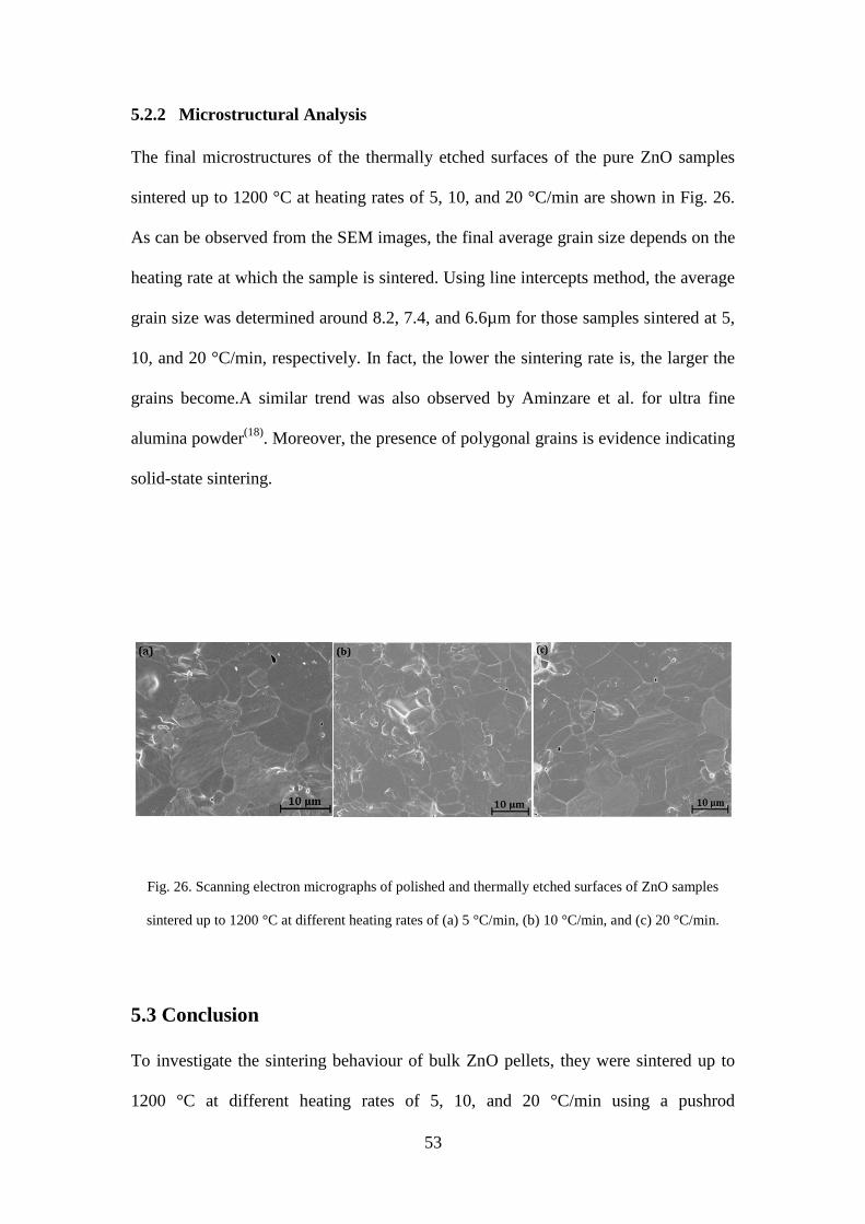
53

5.2.2 Microstructural Analysis The final microstructures of the thermally etched surfaces of the pure ZnO samples

sintered up to 1200 °C at heating rates of 5, 10, and 20 °C/min are shown in Fig. 26.

As can be observed from the SEM images, the final average grain size depends on the

heating rate at which the sample is sintered. Using line intercepts method, the average

grain size was determined around 8.2, 7.4, and 6.6µm for those samples sintered at 5,

10, and 20 °C/min, respectively. In fact, the lower the sintering rate is, the larger the

grains become.A similar trend was also observed by Aminzare et al. for ultra fine

alumina powder(18). Moreover, the presence of polygonal grains is evidence indicating

solid-state sintering.

Fig. 26. Scanning electron micrographs of polished and thermally etched surfaces of ZnO samples

sintered up to 1200 °C at different heating rates of (a) 5 °C/min, (b) 10 °C/min, and (c) 20 °C/min.

5.3 Conclusion To investigate the sintering behaviour of bulk ZnO pellets, they were sintered up to

1200 °C at different heating rates of 5, 10, and 20 °C/min using a pushrod

54

dilatometer. The apparent activation energy was calculated using both the Arhenius

plot and the master sintering curve. However, the values obtained for Q were different

mainly because in contrast to the Arrhenius plot, in which the range of 66%-79% of

relative density was considered, the MSC was constructed over the entire range of

sintering process. Additionally, not only does the heating rate affect the maximum

densification rate, but also the average final grain size. In fact, the higher the heating

rate is, the smaller the final grain size becomes.

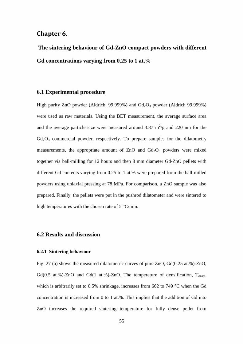
55

Chapter 6. The sintering behaviour of Gd-ZnO compact powders with different

Gd concentrations varying from 0.25 to 1 at.%

6.1 Experimental procedure High purity ZnO powder (Aldrich, 99.999%) and Gd2O3 powder (Aldrich 99.999%)

were used as raw materials. Using the BET measurement, the average surface area

and the average particle size were measured around 3.87 m2/g and 220 nm for the

Gd2O3 commercial powder, respectively. To prepare samples for the dilatometry

measurements, the appropriate amount of ZnO and Gd2O3 powders were mixed

together via ball-milling for 12 hours and then 8 mm diameter Gd-ZnO pellets with

different Gd contents varying from 0.25 to 1 at.% were prepared from the ball-milled

powders using uniaxial pressing at 78 MPa. For comparison, a ZnO sample was also

prepared. Finally, the pellets were put in the pushrod dilatometer and were sintered to

high temperatures with the chosen rate of 5 °C/min.

6.2 Results and discussion

6.2.1 Sintering behaviour Fig. 27 (a) shows the measured dilatometric curves of pure ZnO, Gd(0.25 at.%)-ZnO,

Gd(0.5 at.%)-ZnO and Gd(1 at.%)-ZnO. The temperature of densification, Tonset,

which is arbitrarily set to 0.5% shrinkage, increases from 662 to 749 °C when the Gd

concentration is increased from 0 to 1 at.%. This implies that the addition of Gd into

ZnO increases the required sintering temperature for fully dense pellet from

56

approximately 1000 to 1350 °C. Fig. 27 (b) shows the relative density for the same

sets of samples as a function of temperature. As can be observed from this figure, in

contrast to pure ZnO, in which the shrinkage curve shows no blockage in the sintering

process, the incorporation of Gd2O3 into ZnO results in a suppression of the

densification process. The common shape of these curves reveals that the temperature

at which the densification begins increases by increasing the Gd content in ZnO.

Further, in order to reach a relative density of 90% and above, temperatures above

910, 1065, 1100, and 1243°C are needed for pure ZnO, Gd(0.25 at.%)-ZnO, Gd(0.5

at.%)-ZnO, and Gd(1 at.%)-ZnO, respectively. Fig. 27 (c) indicates the densification

rate as a function of temperature for pure ZnO, Gd(0.25 at.%)-ZnO, Gd(0.5 at.%)-

ZnO, and Gd(1 at.%)-ZnO samples sintered at constant heating rate of 5 °C/min. As

shown in this figure, one peak is observed for the densificaion rate of pure ZnO

sample. However, a second peak appears when Gd is added into ZnO. From the

curves in Fig. 27(c), it is apparent that the intensity of the second peak increases when

the Gd concentration is increased from 0.25 to 1 at.%. Moreover, what is interesting

in these curves is that the densification rate of Gd(1 at.%)-ZnO sample shifts towards

higher temperatures. This significant shift might be due to the higher Gd content,

which leads to more delay for reaching a full dense pellet.

57

Fig. 27. (a) shrinkage versus temperature and (b) relative density versus temperature and (c)

densification rate versus temperature for Gd-ZnO pellets with different Gd contents.

It should be noted that similar suppression of sintering behaviour was observed by

Durazzo et al.(33), Assmann et al.(34), Yuda et al.(35), andSong et al.(36)Manzel et

al.(37)for UO2-Gd2O3 pellets. Hence, there are few papers published on the possible

mechanism for this blockage for the UO2-Gd2O3 system and to the best of our

knowledge no paper has been published yet on the sintering behaviour of Gd-ZnO

system.

According to Manzel et al.(37), the abnormal sintering behaviour observed for the

UO2-Gd2O3 pellets was related to the formation of solid solution occurring

58

simultaneously with the densification process. In fact, the diffusion process taking

place during the sintering process results in two outcomes, densification and the

formation of solid solutions. Hence, the competition between these two processes

leads to reduction in the densification and sintering shift towards higher temperatures,

which is also observed in the Gd-ZnO system. Moreover, based on Durazzo et al.(33),

the formation of low diffusivity phases during the sintering process might have been

the cause of the sintering blockage in the UO2-Gd2O3 system. Therefore, this can be a

possible explanation for why similar behaviour was observed for the Gd-ZnO system,

in which the presence of secondary phase was observed using both the SEM and the

XRD measurements. This mechanism is to referred as the "diffusion barrier

hypothesis"(33).

The crystalline structure of the films was analyzed by XRD using a PANalyticalX'pert

MPD diffractometer, which is equipped with an accelerator detector and operated at

40 kV/40 mA. The XRD spectra for four pellets, pure ZnO Gd(0.25 at.%)-ZnO,

Gd(0.5 at.%)-ZnO, and Gd(1 at.%)-ZnO, are presented in Fig. 28From the XRD

spectra in this figure, in addition to peaks assigned to ZnO with wurtzite hexagonal

structure, another peak is also observed, which corresponds to the (222) plane of the

Gd2O3 crystalline structure. Why Gd3+ ions do not reside at Zn2+ sites may be due to

the marked difference between ionic radii of Gd3+ (0.094nm) and Zn2+(0.074nm) ions.

Thus this difference makes it difficult for Gd3+ ions to substitute for Zn2+ sites.

Moreover, no peak position was observed when Gd2O3 was incorporated into the ZnO

lattice, which may confirm that Gd3+ ions did not reside at Zn2+ sites. However, It

should be borne in mind that the XRD measurement is not sensitive enough to

confirm that whether Gd3+ ions substitute for Zn2+ sites or not. It also should be noted

that the intensity of the peak, which is related toGd

concentration is increased from 0.25 to 1 at.%.

In contrast to our work, in which Gd

al.(33)found a maximum value for the molar fraction of gadolinium beyond which two

or more phases formed in the UO

a linear relationship between the values of the lattice parameters and the amount of

Gd in UO2 below the boundary value, in conformity with Vegard’s law. However, no

linear behaviour was observed beyond this value in the experiments performed in this

study. The reason why Gd

(0.104 nm) is smaller than that of U

U4+ sites.

Fig. 28. XRD patterns of Gd

59

that the intensity of the peak, which is related toGd2O3, increases when the Gd

concentration is increased from 0.25 to 1 at.%.

contrast to our work, in which Gd3+ ions did not substitute for Zn

found a maximum value for the molar fraction of gadolinium beyond which two

or more phases formed in the UO2-Gd2O3 system. According to their report, there was


below the boundary value, in conformity with Vegard’s law. However, no


study. The reason why Gd3+ ions substitute U4+ is because the ionic radius of Gd

aller than that of U4+, therefore it is easy for Gd3+ ions to reside at

Fig. 28. XRD patterns of Gd-ZnO bulk samples containing different Gd concentrations.

, increases when the Gd

ions did not substitute for Zn2+, Durazzo et

found a maximum value for the molar fraction of gadolinium beyond which two

system. According to their report, there was


below the boundary value, in conformity with Vegard’s law. However, no


is because the ionic radius of Gd3+

ions to reside at

ZnO bulk samples containing different Gd concentrations.

60

To understand why the addition of Gd into ZnO inhibits the sintering process, a new

series of samples was prepared under the same conditions. Then, constant heating rate

sintering was carried out on the samples at heating rates ranging from 5 to 20 °C/min.

In the following, the sintering behaviour of Gd-ZnO samples will be discussed, and

then the results will be compared to those obtained from pure ZnO.

Fig. 29 (a)-(c) indicate the densification as a function of temperature for ZnO samples

containing 0.25, 0.5, and 1 at.% of Gd, respectively. The common shape of these

curves, classical sigmoidal shape, reveals that no matter what the heating rate is, the

samples start to densify around 680 °C, which is higher than that of pure ZnO.

Moreover, the temperature, at which the densification starts, increases when the Gd

concentration is increased. This increase suggests that the sinterability of the pellets

deteriorates when the Gd content is increased from 0.25 to 1 at.%. It is also noted that

similar to ZnO, samples sintered at lower heating rate shows higher relative densities.

The effect of heating rate on the temperature at which the densification starts is

presented in Table 3 for ZnO samples containing 0.25, 0.5, and 1 at.%. As can be seen

from the table, a significant shift towards higher temperatures is observed for the

Gd(1 at.%)-ZnO sample indicating the inhibition of sinterability.

61

Fig. 29.relative density versus temperature for (a) Gd(0.25 at.%)-ZnO, (b) Gd(0.5 at.%)-ZnO, and (c)

Gd(1 at.%)-ZnO pellets.

Table 3. Dilatometry data for Gd-ZnO compacts sintered at different heating rates.

Heating rate Gd(0.25 at.%)-ZnO Temperature of onset of

sintering

Gd(0.5 at.%)-ZnO Temperature of

onset of sintering

Gd(1 at.%)-ZnO Temperature of

onset of sintering 5 °C/min 689 °C 716 °C 845 °C

10 °C/min 731 °C 735 °C 873 °C

20 °C/min 753 °C 756 °C 887 °C

62

The densification rate as a function of temperature for Gd(0.25 at.%)-ZnO, Gd(0.5

at.%)-ZnO, and Gd(1 at.%)-ZnO, which were sintered at different heating rates of 5,

10, and 20 °C/min, are shown in Fig. 30 (a)-(c). As shown in these figures and stated

earlier, a second peak appears when Gd2O3 is added into ZnO. Moreover, similar to

pure ZnO, the values of maximum densification rate shift towards higher temperatures

when the heating rate, at which a sample was sintered, is increased from 5 to 20

°C/min (Table 4). Similar behaviour is also observed for the second peak at higher

temperatures.

63

Fig. 30. Densification rate versus temperature for (a) Gd(0.25 at.%)-ZnO, (b) Gd(0.5 at.%)-ZnO, and

(c) Gd(1 at.%)-ZnO pellets.

64

Table 4.Temperatures at which the densification rate for Gd-ZnO compacts sintered at different

heating rates is at a maximum (Tmax)

Heating rate Gd(0.25 at.%)-ZnO

Tmax

Gd(0.5 at.%)-ZnO

Tmax

Gd(1 at.%)-ZnO

Tmax

5 °C/min 842 °C 857 °C 1036 °C

10 °C/min 847 °C 868 °C 1063 °C

20 °C/min 885 °C 873 °C 1071 °C

Fig. 31 (a)-(c) indicate the variation of shrinkage rate, dL/dt, as a function of relative

density for different Gd-ZnO pellets containing 0.25, 0.5, and 1 at.% of Gd2O3, which

were sintered at different heating rates of 5, 10, and 20 °C/min. Similar to pure ZnO

(Fig. 20), a maximum value of instantaneous shrinkage rate in the range of 66%-79%

of relative density, corresponding to the end of neck formation, is observed for all Gd-

ZnO samples. However, a second peak with less intensity appears when Gd2O3 is

added to ZnO. This peak may show a different mechanism, which is not known at this

point. It should be noted that since the Gd(1 at.%)-ZnO sample sintered at 20 °C/min

reaches the final relative density of 85%, no second peak is observed for that. In fact,

this sample should be sintered up to a temperature higher than 1400 °C so as to be less

porous according to the SEM measurement (Fig. 35) and to reach a relative density

higher than 90%.

Fig. 31.relative density versus shrinkage rate for (a) Gd(0.25 at.%)

Gd(1 at.%)

As with the pure ZnO, the apparent activation energies of Gd

calculated using two different methods:

(i)

(ii)

65

Fig. 31.relative density versus shrinkage rate for (a) Gd(0.25 at.%)-ZnO, (b) Gd(0.5 at.%)

Gd(1 at.%)-ZnO pellets sintered at different heating rates.

As with the pure ZnO, the apparent activation energies of Gd-ZnO samples have been

calculated using two different methods:

(i) Arrhenius plot

(ii) Master sintering curve

ZnO, (b) Gd(0.5 at.%)-ZnO, and (c)

ZnO samples have been

(i) Arrhenius plot

The apparent activation energies have been

and 747.0±58.1 KJ/mol for Gd(0.25 at%)

ZnO, respectively using Arrhenius plots of Ln (T

constant rate sintering data

with pure ZnO, in which the apparent activation energy, Q, was estimated around

293.9± 12.8 KJ/mol. This suggests that the addition of Gd

increase in Q. The same trend has been observed by

samples. According to their report

320 KJ/mol to 440 KJ/mol when Mn was added into ZnO.

the variation of activation energy as a function of Gd concentration. As can be

observed from this figure, not only does the activation energy increase, but also

standard deviation.

66

Arrhenius plot

The apparent activation energies have been calculated to be348.0±16.3, 414.6±51.2,

KJ/mol for Gd(0.25 at%)-ZnO, Gd(0.5 at.%)-ZnO, and Gd(1 at.%)

ZnO, respectively using Arrhenius plots of Ln (T

) versus 1/T of the

constant rate sintering data over the range of 66%-79%(Fig. 32 (a)-(c)). In comparison


This suggests that the addition of Gd2O3 into ZnO leads to an

increase in Q. The same trend has been observed by Han et al.(38)for Mn doped ZnO

samples. According to their report(38), the calculated activation energy increased from

320 KJ/mol to 440 KJ/mol when Mn was added into ZnO. Moreover, Fig


observed from this figure, not only does the activation energy increase, but also

standard deviation.

348.0±16.3, 414.6±51.2,

ZnO, and Gd(1 at.%)-

) versus 1/T of thedifferent

. In comparison


into ZnO leads to an

Mn doped ZnO

y increased from

over, Fig. 33 shows


observed from this figure, not only does the activation energy increase, but also the

standard deviation.

Fig. 32. Arrhenius plot of densification data for (a) Gd(0.25 at%)

Gd(1 at.%)-ZnO, sintered a

67

. Arrhenius plot of densification data for (a) Gd(0.25 at%)-ZnO, (b) Gd(0.5 at.%)

ZnO, sintered at different heating rates of 5, 10, and 20 °C/min.

ZnO, (b) Gd(0.5 at.%)-ZnO, and

t different heating rates of 5, 10, and 20 °C/min.

68

Fig. 33.The variation of activation energy versus Gd concentration.

(iii) Master sintering Curve

Master sintering curves were constructed using both the calculated apparent activation

energies (Q) of Gd-ZnO samples and the sintering data. Fig. 34 (a)-(d) indicate the

plots of activation energy versus mean residual square for Gd-ZnO samples sintered at

different heating rates of 5, 10, and 20 °C/min. According to these figures, each curve

has a minimum indicating the best value of apparent activation energy. Therefore, Q

has been estimated around 276, 296, and 462 KJ/mol for Gd(0.25 at.%)-ZnO, Gd(0.5

at.%)-ZnO, and Gd(1 at.%)-ZnO, respectively, which are higher than that of pure ZnO

estimated with the same method (Table 5). Further, these values are different from

those calculated from the Arrhenius plot. In fact, to construct the master sintering

curves the entire range of sintering process has been considered. However, only the

range of 66%-79% of relative density was considered to estimate Q by Arrhenius plot.

69

Table 5. The comparison between the calculated activation energies for Gd-ZnO samples using both

Arrhenius plot and MSC (KJ/mol).

Samples Arrhenius plot

Q KJ/mol

MSC

Q KJ/mol

Pure ZnO 293.9 ± 12.8 24343

Gd(0.25 at.%)-ZnO 348.0 ± 16.3 276

Gd(0.5 at.%)-ZnO 414.6 ± 51.2 296

Gd(1 at.%)-ZnO 747.0 ± 58.1 462

Apparent activation energy, Q (KJ/mol)

71

Fig. 34 .Mean residual squares of error for various values of the activation energy for Gd-ZnO samples

containing 0, 0.25, 0.5, and 1 at.% of Gd2O3.

6.2.2 Microstructural analysis The final microstructure of the thermally etched surfaces of the ZnO pellets with

different Gd concentrations varying from 0.25 to 1 at.% sintered up to 1400 °C at

heating rates of 5, 10, and 20 °C/min are shown in Fig. 35. As can be observed from

SEM images, the final average grain size depends not only on the heating rate, at

which the sample is sintered, but also on the amount of Gd. It is observed that the

average grain size decreases when both the heating rate and the Gd concentration are

increased (Table 6). Additionally, the formation of a secondary phase, which was

confirmed by the XRD analysis, can also be observed by the SEM images as well as

the EDAX measurements (Fig. 36). As can be seen from Fig. 36 (a) and (b), the

72

formation of secondary phase is shown in red color at the surface of Gd(1 at.%)-ZnO

bulk sample heated up to 1400 °C at heating rate of 5 °C/min. Fig. 36 (a) indicates the

EDAX measurement at the surface of the sample where no secondary phase was

detected (where the arrow points toward). However, Fig. 36(b) shows the

measurement at the surface of the same sample where the secondary phase was

formed (where the arrow points toward). As shown, In contrast to Fig. 36(a) in which

no Gd peak is observed, the Gd peak appears in Fig. 36(b) following the noticeable

reduction in the intensity of the Zn peak. Further, the volume fraction of the

secondary phase increases from 14% to 20.5% when the Gd concentration is

increased from 0.25 to 1 at.%.

73

Fig. 35. Scanning electron micrographs of polished and thermally etched surfaces of ZnO samples with

different Gd concentration.

74

Table 6. The effect of Gd concentration and thermal heating rate on the final average grain size (µm).

Heating rate Gd(0.25 at.%)-ZnO Average grain size

(microns)

Gd(0.5 at.%)-ZnO Average grain size

(microns)

Gd(1 at.%)-ZnO Average grain size

(microns) 5 °C/min 20.87 19.95 16.86

10 °C/min 14.96 13.37 11.46

20 °C/min 14.84 11.30 8.60

75

Fig 36. . EDAX measurement at the surface of Gd(1 at.%)-ZnO sample sintered up to 1400 °C at

heating rate of 5 °C/min (a) at the surface of the sample with no secondary phase and (b) at the surface

of the sample with secondary phase.

76

6.3 Conclusion

The addition of Gd2O3 into ZnO affected not only the sintering behaviour, but also the

final microstructure. From the sintering point of view, the incorporation of Gd2O3

into ZnO led to two main results: (i) shifting the required temperatures to obtain fully

dense pellets towards higher values, and (ii) increasing the apparent activation energy.

In addition to sintering behaviour, the final average grain size was also sensitive to the

amount of Gd incorporated into ZnO. In fact, the grain size decreases when the Gd

content is increased.

77

Chapter 7

Thin Film deposition and characterization using the XRD

measurement and SQUID magnetometer

7.1 Target preparation

After determining the appropriate sintering temperature for obtaining fully dense Gd-

ZnO targets, 22 mm diameter Gd-ZnO targets with different Gd contents were

prepared from mixed and ball-milled Gd(0.25 at.%)-ZnO, Gd(0.5 at.%)-ZnO, and

Gd(1 at.%)-ZnO powders pressed and sintered at 1250 °C for 10 h (the measured

target density was higher than 98% for all Gd-ZnO targets).

7.2 Thin film deposition

Before depositing the films, a-plane sapphire (Al2O3 (11-20)) substrates were cleaned

in acetone, isopropanol, and de-ionized water using an ultrasonic bath for 5 minutes

for each step. Gd-ZnO films with different Gd concentrations varying from 0 to 1

at.% were fabricated on clean substrates which were mounted to a resistive heater

using silver paint. The temperature of the substrate was fixed at 650 °C for all films.

The film deposition was performed in a stain-steel vacuum chamber evacuated to a

pressure of 3×10-5Torr. A KrF laser with wavelength of 248 nm was focused on

targets and ablated them. During the deposition, laser frequency, target-substrate

distance and laser beam power density were maintained at 8 Hz, 50 mm, and 0.85

J/cm2, respectively. All films were deposited in oxygen pressure of 50 mTorr. The

number of laser pulses was kept at 10000 pulses.

7.3 Characterization

7.3.1 XRD measurements The crystalline structure of the films was re

a PANalyticalX'pert MPD diffractometer, which is equipped with an accelerator

detector and operated at 40 kV/10 mA.

deposited films with different Gd concentrations varying from 0 to 1 at.% are

presented in Fig. 37 (a) and (b)

no secondary phases, such as Gd

patterns of the corresponding PLD targets, are observed. It is clear that these films

display preferential c-axis orientation, (002) plane. However, a peak corresponding to

the substrate, a-plane sapphire, is also observed at 37.92

Increasing the Gd concentration up to 1 at.% causes a drastic decrease in the intensity

of the (002) diffraction peak and an increase in FWHM, which means that the film

crystallinity degrades (Fig. 37, Fig. 38, and Table 7). Moreover, according to Table

and Fig. 38, the (002) peak position shifts towards higher angles when the Gd

concentration is increased from 0 to 1 at.%. Therefore, the value of c parameter,

determined from the Bragg angle of the (002) peak, decreases.

increasing the Gd concentration could be due to substitution of Gd

network in which Zn2+

electrically neutral, the Gd

as the following mechanism

3Zn

The above mechanism can be rewritten according to the Kroger

78

7.3.1 XRD measurements

The crystalline structure of the films was re-measured and re-analyzed by XRD using


detector and operated at 40 kV/10 mA. The normalized diffraction patterns of


(a) and (b). Within the detection limit of the XRD measurement,

no secondary phases, such as Gd2O3 (at 2Ɵ = 28.6°), which was observed in the XRD


axis orientation, (002) plane. However, a peak corresponding to

plane sapphire, is also observed at 37.92°.



crystallinity degrades (Fig. 37, Fig. 38, and Table 7). Moreover, according to Table



determined from the Bragg angle of the (002) peak, decreases. This reduction with

the Gd concentration could be due to substitution of Gd3+ in ZnO

ions are in tetrahedral sites. Since the ZnO crystal is

electrically neutral, the Gd3+ replacement leads to the formation of cationic vacancies

mechanism (39-41):

3Zn2+ 2GdZn' + VZn2+

The above mechanism can be rewritten according to the Kroger-Vink notation:

0 = 2GdZn' + VZn'

analyzed by XRD using


rmalized diffraction patterns of


. Within the detection limit of the XRD measurement,

was observed in the XRD


axis orientation, (002) plane. However, a peak corresponding to



crystallinity degrades (Fig. 37, Fig. 38, and Table 7). Moreover, according to Table 7



This reduction with

in ZnO wurtzite

ions are in tetrahedral sites. Since the ZnO crystal is

replacement leads to the formation of cationic vacancies

Vink notation:

79

Consequently, the creation of cationic vacancies which are caused by Gd doping

results in the reduction of c-axis length. Similar results were reported in Ce doped

ZnO(39), Er doped ZnO(41), and Gd doped ZnO(40).

Fig. 37. (a)Typical diffraction patterns and (b) (002) peak position of pure ZnO, Gd(0.25 at.%)-ZnO,

Gd(0.5 at.%)-ZnO, and Gd(1 at.%)-ZnO thin films.

80

Fig 38. Change in FWHM and peak position for pure ZnO Gd(0.25 at.%)-ZnO, Gd(0.5 at.%)-ZnO, and

Gd(1 at.%)-ZnO thin films.

Table 7. Peak position, FWHM, and C lattice parameter obtained from XRD data

Gd concentration (at.%) Peak Position

(degree)

FWHM (degree) Lattice parameter c (A°)

0 34.58 0.117 5.182

0.25 34.77 0.208 5.154

0.5 34.73 0.313 5.159

1 34.73 0.383 5.159

7.3.2 Magnetization

Figures 39(a)-39(c) present the M-H curves of the pure ZnO, Gd(0.25 at.%)-ZnO, and

Gd(0.5 at.%)-ZnO measured at 5 and 300 K. As shown in the figures, the films reveal

diamagnetic behaviour even after substrate subtraction. It is worth noting that the

centre portion of the raw data (insert in Fig 39(a)) in the M

like behaviour with a negative slope. In contrast, the raw data of the films containing

1 at.% of Gd exhibits the loop like behaviour. Here, to eliminate the diamagnetic

contribution of the a-plane sapphire, the following procedure was adopted: at a very

low temperature (5K) and a very high field (50kOe) at which the diamagnetic

contribution of the substrate is too high, the data were corrected by equalizing a slope

to the slope of the magnetization loop. The same procedure was followed to modify

the magnetization curve at 300 K. The magnetization curve reveals a super

paramagnetic like behaviour at 5 K whereas a saturated magnetization at 300 K (Fig.

40). At 300 K, the magnetization curve is characterized with a saturation

magnetization (Ms) 2.19×10

emu/g, and coercive field (H

emu/g, (Mr) 3.24×10-5

than those at 300 K. It is worth notin

behaviour could be due to segregation of secondary phase or due to un

Hence, further experiments need to be conducted to eliminate any secondary pha

81

centre portion of the raw data (insert in Fig 39(a)) in the M-H curves show a linear

ke behaviour with a negative slope. In contrast, the raw data of the films containing


plane sapphire, the following procedure was adopted: at a very

temperature (5K) and a very high field (50kOe) at which the diamagnetic



ation curve at 300 K. The magnetization curve reveals a super



2.19×10-4 emu/g, remanent magnetization (M

emu/g, and coercive field (HC) 75 Oe. At 5 K, the values of (M

emu/g, and (HC) 125 Oe are obtained, which

than those at 300 K. It is worth noting that the observed super-paramagnetic like

behaviour could be due to segregation of secondary phase or due to un-

Hence, further experiments need to be conducted to eliminate any secondary pha

H curves show a linear

ke behaviour with a negative slope. In contrast, the raw data of the films containing


plane sapphire, the following procedure was adopted: at a very

temperature (5K) and a very high field (50kOe) at which the diamagnetic



ation curve at 300 K. The magnetization curve reveals a super-



emu/g, remanent magnetization (Mr) 2.08×10-5

75 Oe. At 5 K, the values of (Ms) 2.22×10-3

125 Oe are obtained, which are higher

paramagnetic like

-reacted Gd2O3.

Hence, further experiments need to be conducted to eliminate any secondary phases.

82

Fig 39. M versus H curves of pure ZnO (a), Gd(0.25 at.%)-ZnO (b), and Gd(0.5 at.%)-ZnO (c) thin

films measured at 5 and 300 K.

Fig 40. Magnetization hysteresis curves of the Gd(1 at.%)

7.4 Summary and future work Gd-ZnO films with different Gd concentrations varying from 0 to 1 at.%

prepared by pulsed laser deposition (PLD). According to the XRD analysis, all films

exhibit preferential c-axis orientation, (0 0 2) orientation. Further, the (0 0 2) peak

position shifts towards the higher angle when the Gd concentration is increase

0 to 1 at.%. Moreover, no secondary phase is observed in the XRD plots; however, it

does not guarantee that Gd ions reside at Zn

83

Fig 40. Magnetization hysteresis curves of the Gd(1 at.%)-ZnO thin film measured at 5 and 300 K

7.4 Summary and future work

ZnO films with different Gd concentrations varying from 0 to 1 at.%


axis orientation, (0 0 2) orientation. Further, the (0 0 2) peak

position shifts towards the higher angle when the Gd concentration is increase


does not guarantee that Gd ions reside at Zn2+ sites in the ZnO lattice because the X

measured at 5 and 300 K

ZnO films with different Gd concentrations varying from 0 to 1 at.% were


axis orientation, (0 0 2) orientation. Further, the (0 0 2) peak

position shifts towards the higher angle when the Gd concentration is increased from


in the ZnO lattice because the X-

84

ray diffraction is not sensitive enough to detect and analyze precipitates of dopants in

ZnO, here Gd, with Gd content lower than 10 at.%. Additionally, Magnetic

measurements of the Gd-ZnO films with different Gd concentrations varying from 0

to 0.5 at% revealed a diamagnetic characteristic at both 5 and 300K; however, a film

containing 1 at.% of Gd indicated a super-paramagnetic like behaviour at 5 K

whereas a saturated magnetization at 300 K.

It is absolutely crucial that the room temperature ferromagnetic (RTFM) behaviour of

diluted-magnetic semiconductors is intrinsic. In fact, it is ideal that this property does

not originate from extrinsic effects, such as ferromagnetic precipitate and impurity

phases. Hence, several techniques, such as SEM, TEM, XPS, etc should be utilized to

eliminate the possible impurity phases.

Additionally, for possible practical applications it is necessary to have reproducible

RTFM films. However, RTFM behaviour is sensitive to the conditions under which

the thin films are deposited. Therefore, ZnO films containing different dopants need

to be deposited under various growth conditions, such as different oxygen pressures

and substrate temperatures. For comparison, it is worth doping ZnO films with both

rare earth metals as well as transition metals.

85

References

1. Maekawa S. Concepts in Spin Electronics. Oxford: Oxford University Press;

2006.

2. Prellier W, Fouchet A, Mercey B. Oxide-diluted magnetic semiconductors: a

review of the experimentsl status. J Phys: Condens Matter 2003;15:1583-601.

3. CA. Chambers S ,F.C. Forrow R. New Possibilities for Ferromagnetic

Semiconductors. MRS BULLETIN. 2003:729-33.

4. Dietl T, Ohno H, Matsukura F, Cibert J, Ferrand D. Zener model description

of ferromagnetism in zinc-blende magnetic semiconductors. Science. 2000;287:1019-

22.

5. Quesada A, Garcia MA, de la Venta J, Fernandez Pinell E, Merino JM,

Hernando A. Ferrmagnetic behaviour in semiconductors: a new magnetism in search

of spintronic materials. EurPhys J B. 2007;59:457-61.

6. Fukumura T, Yamada Y, Toyosaki H, Hasegawa T ,Koinuma H, Kawasaki M.

Exploration of oxide-based diluted magnetic semiconductors toward transparent

spintronics. Applied Surface Science. 2004;223:62–7.

7. Yousefi M, Azimirad R, Amiri M, Moshfegh AZ. Effect of annealing

temperature on growth of Ce-ZnOnanocomposite thin films: X-ray photoelectron

spectroscopy study. Thin Solid Films. 2011;in press

8. Dutta M, Mridha S, Basak D. Effect of sol concentration on the properties of

ZnO thin films prepared by sol–gel technique. Applied Surface Science.

2008 ;254:2743–7.

9. Santos AMP, Santos EJP. Pre-heating temperature dependence of the c-axis

orientation of ZnO thin films.Thin Solid Films. 2008;516:6210–4.

86

10. Getzlaff M. Fundamentals of magnetism Berlin: Springer-Verlag; 2008.

11. Nolting W, Ramakanth A .Quantum theory of magnetism. Berlin; London:

Springer; 2009.

12. Aminzare M. Investigation on Sintering Behavior of Nano Alumina and Effect

of Conformation Methods on Microstructure and Mechanical Properties. Tehran: Iran

University of Science and Technology; March 2011.

13. Rahman MN. Ceramic Processing and Sintering New York: CRC Press; 2003.

14. N. Calata J. DenisificationBehavior of Ceramic and Crystallizable Glass

Materials Constrained on a Rigid Substrate

Virginia: Virginia Polytechnic Instituteand State University; 2005.

15. Hunghai S, Johnson DL. Master Sintering Curve: A Practical Approacj to

Sintering. Journal of American Ceramics Society. 1996;79:3211-17.

16. Kutty TRG, Khan KB, Hegde PV, J. Banerjee a, Sengupta AK, Majumdar S,

et al. Development of a master sintering curve for ThO2. Journal of Nuclear

Materials. 2004;327:211–9.

17. Mao-HuaTeng, Yi-Chun Lai, Chen Y-T. A Computer Program of Master

Sintering Curve: Model to Accurately Predict Sintering Results. Western Pacific

Earth Sciences .2002;2:171-80.

18. Aminzare M, Mazaheri M, Golestani-fard F, Rezaie HR, Ajeian R. Sintering

behavior of nano alumina powder shaped by pressure filtration. Ceramics

International. 2011;37:9-11.

19. Frederic IsingizweNturambirwe J. Superconducting Quantum Interference

Device (SQUID) Magnetometers: Principles, Fabrication and Applications: African

Institute for Mathematical Sciences (AIMS); 2010.

87

20. ; Available from: http://hyperphysics.phy-

astr.gsu.edu/hbase/quantum/xtube.html.

21. Lauren A., Josephson Effec, University of California Berkley; 2007.

22. SQUID magnetometer. London2009; Available from:

http://www.npl.co.uk/quantum-phenomena/nanophysics/research/squid-

magnetometer.

23. Akram R. Fabrication and optimization of rf-SQUID and Integration assembly

for high resolution magnetic imaging system: BilkentUniversit; 2005.

24. Bäuerle D. Laser processing and chemistry Berlin ; London: Springer; 2000.

25. Mario B. Thin Film Analysis by X-Ray Scattering: Wiley-VCH Verlag,

GmbH & Co. .

26. Birkholz M. Thin Film Analysis by X-ray scattering: Wiley-VCH.

27. Kittel C. Introduction to solid state physics NewYork: Wiley; 2005.

28. Principles of Push-rod Dilatometry. Available from:

http://www.anter.com/TN69.htm.

29. Jena A, K. G. A Novel Technique for Surface Area and Particle Size

Determination of Components of Fuel Cells and Batteries

Cornell Business and Technology Park, Porous Materials I.

30. M. Aminzarea, F. Golestani-farda, O. Guillonb, Mehdi Mazaheri, Rezaie HR.

Sintering behavior of an ultrafine alumina powder shaped by pressure filtration

and dry pressing. Materials Science and Engineering A. 2010;527:3807–12.

31. Guillaume B-G, Christian G. Apparent Activation Energy for the

Densification of a Commercially Available Granulated Zirconia Powder. Journal of

American Ceramics Society .2007;90:1246–50.

88

32. Kevin GE, Donald TE. Analysis of Nanocrystalline and Microcrystalline ZnO

Sintering Using Master Sintering Curves.Journal of American Ceramics Society.

2006;89:2003–9.

33. M. Durazzo, F.B.V. Oliveira, E.F. Urano de Carvalho, Riella .HG. Phase

studies in the UO2–Gd2O3 system. Journal of Nuclear Materials. 2010;400:183–8.

34. H. Assmann, M. Peehs, Roepenack H. Survey of Binary Oxide Fuel

Manufacturing Aan Quality Control. Journal of Nuclear Materials. 1988;153:115-26.

35. Ryoichi Yuda ,Une K. Effect of sintering atmosphere on the densification of

U02-Gd203 compacts. Journal of Nuclear Materials. 1991;178:195-203.

36. K. W. Song, K. S. Kim, K. J. Yang, K. W. Kang, Jung YH. A mechanism for

the sintered density decrease of UO2-Gd2O3 pellets under an oxidizing

atmosphere.Journal of Nuclear Materials. 2001;288:92-9.

37. R. Manzel, Dörr; W. American Ceramics Society

1980;59:601.

38. Jiaping Han, Senos AMR, Mantas PQ. Nonisothermal Sintering of Mn Doped

ZnO.Journal of the European CeramicSociety. 1999;19:1003-6.

39. Sifiani Z, Derkowska B, Dalasinski P, Wojdyla M, Dabos-Seignon S,

AlaouiLamrani M, et al. Optical properties of ZnO and ZnO:Ce layers grown by spray

pyrolysis. Optics Communications. 2006;267:433–9.

40. Subramanian M, ThakurP, Tanemura M, Hihara T, Ganesan V, Soga T, et al.

Intrinsic ferromagnetism and magnetic anisotropy in Gd-doped ZnO thin films

synthesized by pulsed spray pyrolysis method. Journal of Applied Physics.

2010;108(5):053904.

89

41. Pérez-Casero R, Gutiérrez-Llorente A, Pons-Y-Moll O, Seiler W, Marie

Defourneau R, Defourneau D, et al. Er-doped ZnO thin films grown by pulsed-laser

deposition. Journal of Applied Physics. 2005;94:054905.

Sintering of ZnO-Gd 2O3 ceramic targets for functional ...

Documents

Transcript of Sintering of ZnO-Gd 2O3 ceramic targets for functional ...