Sinkhorn Networks: Using Optimal TransportTechniques to Learn Permutations

Gonzalo Mena1∗, David Belanger2, Gonzalo Muñoz3, Jasper Snoek2

1. Columbia University, New York, NY, USA.2. Google Brain, Cambridge, MA, USA.

3. Polytechnique Montréal, Montréal, Québec, Canada.

Abstract

Recently, Optimal Transport (OT) has received significant attention in the MachineLearning community. It has been shown to be useful as a tool for generativemodeling, in which the density estimation problem is cast as the minimizationof a linear function on the transportation polytope. Entropy regularization ofthis problem (Cuturi, 2013) has been demonstrated to be particularly useful, asits solution can be characterized in terms of the Sinkhorn operator, which i) canbe computed more efficiently than the original problem and ii) enables efficientautomatic differentiation (AD). We show that this technique extends to the Birkhoffpolytope, and we use it to understand the solution of the linear assignment problemas a limit of the Sinkhorn operator. This observation justifies and enables the use ofAD in computation graphs containing permutations as intermediate representations.As a result, we are able to introduce Sinkhorn networks for learning permutations,extending the work of Adams & Zemel (2011), and apply them to a variety of tasks.The success of our extension suggests entropy regularization might be used in otherpolytopes as well, enabling AD in other discrete structures.

1 Introduction

Optimal Transport (OT) Villani (2003) has received increased interest among the Machine Learningcommunity, as it provides a renewed perspective to the question on how to compare two distributions.Indeed, the interpretation of the OT program as the minimum amount of total mass moved inorder to transform one distribution into another Arjovsky et al. (2017) provides two advantagesover the classical information paradigm for learning, based on minimization of KL divergence (e.g.maximum likelihood): first, it is not ill-posed when the true distribution lies on a low-dimensionalmanifold (Montavon et al., 2016; Genevay et al., 2017), and second, it provides a rich parameterizationof the distance between distributions, given by the ‘schedule’ that minimizes the moved mass, thetransportation plan.

The main drawback to applying OT is that it requires solving a linear problem that, although havingpolynomial complexity, in practice entails a substantial computational burden. An appealing solutionwas proposed by Cuturi (2013), where the original problem is replaced by an entropy-regularizedversion, whose solution is shown to be equivalent to the application of the so-called Sinkhorn operator(Sinkhorn, 1964), with a reduced computational cost. Since then, entropy regularization has gainedpopularity among practitioners, and more recently, has enabled automatic differentiation (AD) for thetraining of generative models based on OT Genevay et al. (2017), thanks to the differentiability of theSinkhorn operator.

∗gem2131@columbia.edu, Work done during an internship at Google Brain, Cambridge, MA.

31st Conference on Neural Information Processing Systems (NIPS 2017), Long Beach, CA, USA.

In this work, we extend this entropy regularization technique to show that the solution of thelinear assignment problem can also be approximated with the Sinkhorn operator, enabling AD incomputation graphs containing parameterized permutations as intermediate nodes, by replacing themby their differentiable approximations (section 2). Notably, by doing this we introduce Sinkhornnetworks (section 3) which are able to learn the right permutation from training examples. We applySinkhorn networks to a variety of tasks, where we achieve state-of-the-art results (section 4).

2 An analog of the softmax for permutations

In this section we state our theoretical contribution, a rule to approximate matchings with the Sinkhornoperator, based on entropy regularization. We motivate it as an extension of a most elementary,discrete case, and defer a discussion of its relation to OT to section 5.

One sensible way to approximate a discrete category by continuous values is by us-ing temperature-dependent softmax function, component-wise defined as softmaxτ (xi) =exp(xi/τ)/

∑j=1 exp(xj/τ). For positive values of τ , softmaxτ (xi) is a point in the probabil-

ity simplex. Also, in the limit τ → 0, softmaxτ (xi) converges to a vertex of the simplex, a one-hotvector, corresponding to the largest xi 2. This approximation is a key ingredient in the successfulimplementations by (Jang et al., 2016; Maddison et al., 2016), to enable AD in computation graphscontaining discrete nodes, and here we extend it to permutations.

To do so, we first note that the Sinkhorn operator (the iterative normalization of rows and columns ofa matrix) is an analogue of the softmax, for permutations. Specifically, for an N dimensional matrixX , we define 3 Tr(X) = X � (X1N1>N ), and Tv(X) = X � (1N1>NX) as the row and column-wisenormalization operators of a matrix, with � denoting the element-wise division and 1N a columnvector of ones. Then, we define the Sinkhorn operator S(·) as follows:

S0(X) = exp(X), (1)

Sm(X) = Tc(Tr(Sn−1(X))

),

S(X) = limm→∞

Sm(X).

A theorem due to (Sinkhorn, 1964) 4 , proves that S(X) must belong to the Birkhoff polytope, the setof doubly stochastic matrices, that we denote BN .

To continue our analogy with categories, first notice that choosing a category can always be cast as amaximization problem: the choice argmaxi xi is the one that maximizes the function 〈x, v〉 (with vbeing a one-hot vector), since the maximizing v∗ is the one that indexes the largest xi. By parallelingthis construction, one may parameterize the choice of a permutation P through a matrix X , as thesolution to the linear assignment problem (Kuhn, 1955), with PN denoting the set of permutationmatrices:

M(X) = arg maxP∈PN

trace(P>X). (2)

Our theoretical contribution is to notice that the hard choice of a permutation, M(X), can be obtainedas the limit of S(X/τ), meaning that one can approximate M(X) ≈ S(X/τ) with a small τ .Theorem 1 summarizes our finding. We provide a rigorous proof in Appendix A, where we alsocomment on its relation to the simpler discrete case. This proof is based on showing that S(X/τ)solves a certain entropy-regularized problem in Bn, which in the limit converges to the matchingproblem in equation 2.

Theorem 1. For a doubly-stochastic matrix P , define its entropy as h(P ) = −∑i,j Pi,j log (Pi,j).

Then, one has,S(X/τ) = arg max

P∈BN

trace(P>X) + τh(P ). (3)

Now, assume also the entries of X are drawn independently from a distribution that is absolutelycontinuous with respect to the Lebesgue measure in R. Then, almost surely, the following convergence

2Unless the degenerate case of ties.3Notation borrowed from Adams & Zemel (2011)4This theorem requires certain technical conditions which are trivially satisfied if X has positive entries,

motivating the use of the component-wise exponential exp(·) in the first line of equation 1.

2

holds:M(X) = lim

τ→0+S(X/τ). (4)

3 Sinkhorn Networks

Now we show how to apply the approximation stated in Theorem 1 in the context of artificial neuralnetworks. We construct a layer that encodes the representation of a permutation, and show how totrain networks containing such layers as intermediate representations.

We define the components of this network through a minimal example: consider the supervised taskof learning a mapping from scrambled objects X̃ to actual, non-scrambled X . Data, then, are Mpairs (Xi, X̃i) where X̃i can be constructed by randomly permuting pieces of Xi. We state thisproblem as a permutation-valued regression Xi = π−1

θ,X̃i

(X̃i

)+ εi, where εi is a noise term, and

πθ,X̃iis the permutation (represented as a matrix) that maps Xi to X̃i, and that depends on X̃i and

some parameters θ. We are concerned with minimization of the reconstruction error 5:

f(θ,X, X̃) =

M∑i=1

||Xi − π−1θ,X̃i

(X̃i

)||2. (5)

One way to express a complex parameterization of this kind is through a neural network: this networkreceives X̃i as input, which is then passed through some intermediate, feed-forward computations ofthe type gl(Wlxl+bl), where gl are nonlinear activation functions, xl is the output of a previous layer,and θ = {(Wl, bl)} are the network parameters. To make the final network output be a permutation,we appeal to constructions developed in section 2: by assuming that the final network output πθ,X̃can be parameterized as the solution of the assignment problem; i.e., πθ,X̃

(X̃)= M(g(X̃, θ)),

where g(X̃, θ) is the output of the computations involving fl.

Unfortunately, the above construction involves a non-differentiable f (in θ). We use Theorem 1as a justification for replacing M(g(X̃, θ)) by the differentiable S(g(X̃, θ)/τ) in the computationgraph. The value of τ must be chosen with caution: if τ is too small, gradients vanishes almosteverywhere, as S(g(X̃, θ)/τ) approaches the non-differentiable M(g(X̃, θ)). Conversely, if τ is toolarge, S(X/τ) may be far from the vertices of the Birkhoff polytope, and reconstructions π−1

θ,X̃

(X̃)

may be nonsensical (see Figure 1a). Importantly, we will always add noise to the output layer g(X̃, θ)as a regularization device: by doing so we ensure uniqueness of M(g(X̃, θ)), which is required forconvergence in Theorem 1.

3.1 Permutation equivariance

Among all possible architectures that respect the aforementioned parameterization, we will onlyconsider networks that are permutation equivariant, the natural kind of symmetry arising in thiscontext. Specifically, we require networks to satisfy:

πθ,π′(X̃)

(π′(X̃)

)= π′

(πθ(X̃

),

where π′ is an arbitrary permutation. The underlying intuition is simple: reconstructions of objectsshould not depend on how pieces were scrambled, but only on the pieces themselves. We achievepermutation equivariance by using the same network to process each piece of X̃ , which we requireto have an N dimensional output. Then, these N outputs (each with N components) are used toconform the rows of the matrix g(X̃, θ), to which we finally apply the (differentiable) Sinkhornoperator. One can interpret each row as representing a vector of local likelihoods of assignment, butthey might be inconsistent. The Sinkhorn operator, then, mixes those separate representations aremixed, and ensures that consistent (approximate) assignment are produced.

5This error arises from gaussian εi. Other choices may be possible, but here we stick to the straightestformulation

3

N = 80 N = 100 N = 120

Test distribution P.W. P.A.W. P.W. P.A.W. P.W. P.A.W.

U(0, 1) .0 .0 .0 .0 .0 .01U(0, 10) .0 .0 .0 .02 .0 .03U(0, 1000) .0 .01 .0 .02 .0 .04U(1, 2) .0 .01 .0 .04 .0 .08U(10, 11) .0 .08 .0 .08 .1 .6U(100, 101) .02 .65 .09 .99 .12 1.U(1000, 1001) .22 1. .39 1. .49 1.

Table 1: Results in the number sorting task, for test data sampled from different uniform distributions.∗Results from Vinyals et al. (2015)

With permutation equivariance, the only consideration that will be left to the practitioner is thechoice of the particular architecture, which will depend on the particular kind of data. In Section 4we illustrate the uses of Sinkhorn Networks with three examples, each of them using a differentarchitecture.

4 Experiments

4.1 Sorting numbers

To illustrate the capabilities of Sinkhorn Networks in the most elementary case, we considered thetask of sorting numbers using artificial neural networks, first described in (Vinyals et al., 2015).Specifically, we sample uniform random numbers X̃ in the [0, 1] interval and we train our networkwith pairs (X̃,X) where X are the same X̃ but in order. The network has a first fully connectedlayer that links a number with an intermediate representation (with 32 units), and a second (also fullyconnected) layer that turns that representation into a row of the matrix g(X̃, θ).

Table 1 shows our network learns to sort up to N = 120 numbers. We used two evaluation measures:the proportion of wrong responses (P.W.), and the proportion of sequences where there was at leastone error (P.A.W.). Surprisingly, the network learns to sort number even when test examples arenot sampled from U(0, 1), but on a considerably different interval. This indicates the network is notoverfitting. These results may be compared with the ones in Vinyals et al. (2015), where a muchmore complex (recurrent) network was used, but performance guarantees were obtained only withat most N = 15 numbers. In that case, the reported P.A.W is 0.9, ours is negligible for most testdistributions.

4.2 Jigsaw Puzzles

A more complex scenario for learning a permutation relates to images, which has been addressedin (Noroozi & Favaro, 2016; Cruz et al., 2017). There, we would like to solve a Jigsaw puzzle, torecover an image X given their scrambled pieces X̃ , at a certain level of atomicity. In this example,our network differs from the one in 4.1 slightly: now, the first layer is a simple CNN (convolution +max pooling), which maps the puzzle pieces to an intermediate representation.

For evaluation on test data we report l1 and l2 (train) losses and the Kendall tau, a ‘correlationcoefficient’ for ranked data. In Table 2 we benchmark results for the MNIST, Celeba and Imagenetdatasets, with puzzles between 2x2 and 6x6 pieces. In MNIST we achieve very low l1 and l2 errorson up to 6x6 puzzles, although a high proportion of errors. This is a consequence of our loss beingagnostic to particular permutations, but only caring about reconstruction errors: as the number ofblack pieces increases with the number of puzzle pieces, most of them become unidentifiable underthis loss.

In Celeba, we are able to solve puzzles of up to 5x5 pieces with only 21% of pieces of faces beingincorrectly ordered (see Figure 1a for examples of reconstructions). However, learning in the theImagenet dataset is much more challenging, as there isn’t a sequential structure that generalizesamong images, unlike Celeba and MNIST. In this dataset, our network ties with the .72 Kendall tau

4

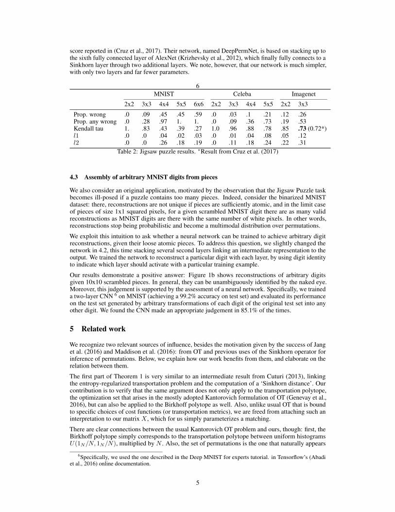
score reported in (Cruz et al., 2017). Their network, named DeepPermNet, is based on stacking up tothe sixth fully connected layer of AlexNet (Krizhevsky et al., 2012), which finally fully connects to aSinkhorn layer through two additional layers. We note, however, that our network is much simpler,with only two layers and far fewer parameters.

6MNIST Celeba Imagenet

2x2 3x3 4x4 5x5 6x6 2x2 3x3 4x4 5x5 2x2 3x3

Prop. wrong .0 .09 .45 .45 .59 .0 .03 .1 .21 .12 .26Prop. any wrong .0 .28 .97 1. 1. .0 .09 .36 .73 .19 .53Kendall tau 1. .83 .43 .39 .27 1.0 .96 .88 .78 .85 .73 (0.72*)l1 .0 .0 .04 .02 .03 .0 .01 .04 .08 .05 .12l2 .0 .0 .26 .18 .19 .0 .11 .18 .24 .22 .31

Table 2: Jigsaw puzzle results. ∗Result from Cruz et al. (2017)

4.3 Assembly of arbitrary MNIST digits from pieces

We also consider an original application, motivated by the observation that the Jigsaw Puzzle taskbecomes ill-posed if a puzzle contains too many pieces. Indeed, consider the binarized MNISTdataset: there, reconstructions are not unique if pieces are sufficiently atomic, and in the limit caseof pieces of size 1x1 squared pixels, for a given scrambled MNIST digit there are as many validreconstructions as MNIST digits are there with the same number of white pixels. In other words,reconstructions stop being probabilistic and become a multimodal distribution over permutations.

We exploit this intuition to ask whether a neural network can be trained to achieve arbitrary digitreconstructions, given their loose atomic pieces. To address this question, we slightly changed thenetwork in 4.2, this time stacking several second layers linking an intermediate representation to theoutput. We trained the network to reconstruct a particular digit with each layer, by using digit identityto indicate which layer should activate with a particular training example.

Our results demonstrate a positive answer: Figure 1b shows reconstructions of arbitrary digitsgiven 10x10 scrambled pieces. In general, they can be unambiguously identified by the naked eye.Moreover, this judgement is supported by the assessment of a neural network. Specifically, we traineda two-layer CNN 6 on MNIST (achieving a 99.2% accuracy on test set) and evaluated its performanceon the test set generated by arbitrary transformations of each digit of the original test set into anyother digit. We found the CNN made an appropriate judgement in 85.1% of the times.

5 Related work

We recognize two relevant sources of influence, besides the motivation given by the success of Janget al. (2016) and Maddison et al. (2016): from OT and previous uses of the Sinkhorn operator forinference of permutations. Below, we explain how our work benefits from them, and elaborate on therelation between them.

The first part of Theorem 1 is very similar to an intermediate result from Cuturi (2013), linkingthe entropy-regularized transportation problem and the computation of a ‘Sinkhorn distance’. Ourcontribution is to verify that the same argument does not only apply to the transportation polytope,the optimization set that arises in the mostly adopted Kantorovich formulation of OT (Genevay et al.,2016), but can also be applied to the Birkhoff polytope as well. Also, unlike usual OT that is boundto specific choices of cost functions (or transportation metrics), we are freed from attaching such aninterpretation to our matrix X , which for us simply parameterizes a matching.

There are clear connections between the usual Kantorovich OT problem and ours, though: first, theBirkhoff polytope simply corresponds to the transportation polytope between uniform histogramsU(1N/N, 1N/N), multiplied by N . Also, the set of permutations is the one that naturally appears

6Specifically, we used the one described in the Deep MNIST for experts tutorial. in Tensorflow’s (Abadiet al., 2016) online documentation.

5

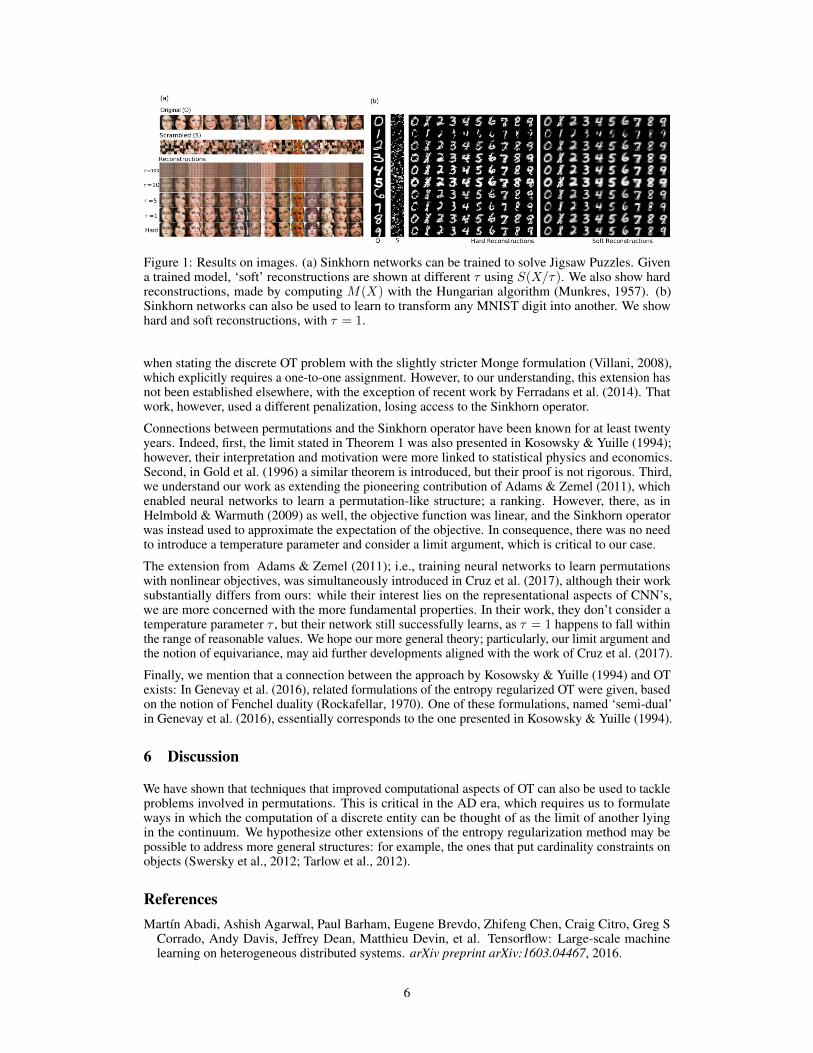
Figure 1: Results on images. (a) Sinkhorn networks can be trained to solve Jigsaw Puzzles. Givena trained model, ‘soft’ reconstructions are shown at different τ using S(X/τ). We also show hardreconstructions, made by computing M(X) with the Hungarian algorithm (Munkres, 1957). (b)Sinkhorn networks can also be used to learn to transform any MNIST digit into another. We showhard and soft reconstructions, with τ = 1.

when stating the discrete OT problem with the slightly stricter Monge formulation (Villani, 2008),which explicitly requires a one-to-one assignment. However, to our understanding, this extension hasnot been established elsewhere, with the exception of recent work by Ferradans et al. (2014). Thatwork, however, used a different penalization, losing access to the Sinkhorn operator.

Connections between permutations and the Sinkhorn operator have been known for at least twentyyears. Indeed, first, the limit stated in Theorem 1 was also presented in Kosowsky & Yuille (1994);however, their interpretation and motivation were more linked to statistical physics and economics.Second, in Gold et al. (1996) a similar theorem is introduced, but their proof is not rigorous. Third,we understand our work as extending the pioneering contribution of Adams & Zemel (2011), whichenabled neural networks to learn a permutation-like structure; a ranking. However, there, as inHelmbold & Warmuth (2009) as well, the objective function was linear, and the Sinkhorn operatorwas instead used to approximate the expectation of the objective. In consequence, there was no needto introduce a temperature parameter and consider a limit argument, which is critical to our case.

The extension from Adams & Zemel (2011); i.e., training neural networks to learn permutationswith nonlinear objectives, was simultaneously introduced in Cruz et al. (2017), although their worksubstantially differs from ours: while their interest lies on the representational aspects of CNN’s,we are more concerned with the more fundamental properties. In their work, they don’t consider atemperature parameter τ , but their network still successfully learns, as τ = 1 happens to fall withinthe range of reasonable values. We hope our more general theory; particularly, our limit argument andthe notion of equivariance, may aid further developments aligned with the work of Cruz et al. (2017).

Finally, we mention that a connection between the approach by Kosowsky & Yuille (1994) and OTexists: In Genevay et al. (2016), related formulations of the entropy regularized OT were given, basedon the notion of Fenchel duality (Rockafellar, 1970). One of these formulations, named ‘semi-dual’in Genevay et al. (2016), essentially corresponds to the one presented in Kosowsky & Yuille (1994).

6 Discussion

We have shown that techniques that improved computational aspects of OT can also be used to tackleproblems involved in permutations. This is critical in the AD era, which requires us to formulateways in which the computation of a discrete entity can be thought of as the limit of another lyingin the continuum. We hypothesize other extensions of the entropy regularization method may bepossible to address more general structures: for example, the ones that put cardinality constraints onobjects (Swersky et al., 2012; Tarlow et al., 2012).

ReferencesMartín Abadi, Ashish Agarwal, Paul Barham, Eugene Brevdo, Zhifeng Chen, Craig Citro, Greg S

Corrado, Andy Davis, Jeffrey Dean, Matthieu Devin, et al. Tensorflow: Large-scale machinelearning on heterogeneous distributed systems. arXiv preprint arXiv:1603.04467, 2016.

6

Ryan Prescott Adams and Richard S Zemel. Ranking via sinkhorn propagation. arXiv preprintarXiv:1106.1925, 2011.

Martin Arjovsky, Soumith Chintala, and Léon Bottou. Wasserstein gan. arXiv preprintarXiv:1701.07875, 2017.

Garrett Birkhoff. Tres observaciones sobre el algebra lineal. Univ. Nac. Tucumán. Revista A, 5:147–151, 1946.

Rodrigo Santa Cruz, Basura Fernando, Anoop Cherian, and Stephen Gould. Deeppermnet: Visualpermutation learning. arXiv preprint arXiv:1704.02729, 2017.

Marco Cuturi. Sinkhorn distances: Lightspeed computation of optimal transport. In Advances inneural information processing systems, pp. 2292–2300, 2013.

Sira Ferradans, Nicolas Papadakis, Gabriel Peyré, and Jean-François Aujol. Regularized discreteoptimal transport. SIAM Journal on Imaging Sciences, 7(3):1853–1882, 2014.

Aude Genevay, Marco Cuturi, Gabriel Peyré, and Francis Bach. Stochastic optimization for large-scale optimal transport. In Advances in Neural Information Processing Systems, pp. 3440–3448,2016.

Aude Genevay, Gabriel Peyré, and Marco Cuturi. Sinkhorn-autodiff: Tractable wasserstein learningof generative models. arXiv preprint arXiv:1706.00292, 2017.

Steven Gold, Anand Rangarajan, et al. Softmax to softassign: Neural network algorithms forcombinatorial optimization. Journal of Artificial Neural Networks, 2(4):381–399, 1996.

David P Helmbold and Manfred K Warmuth. Learning permutations with exponential weights.Journal of Machine Learning Research, 10(Jul):1705–1736, 2009.

Eric Jang, Shixiang Gu, and Ben Poole. Categorical reparameterization with gumbel-softmax. arXivpreprint arXiv:1611.01144, 2016.

JJ Kosowsky and Alan L Yuille. The invisible hand algorithm: Solving the assignment problem withstatistical physics. Neural networks, 7(3):477–490, 1994.

Alex Krizhevsky, Ilya Sutskever, and Geoffrey E Hinton. Imagenet classification with deep convolu-tional neural networks. In Advances in neural information processing systems, pp. 1097–1105,2012.

Harold W Kuhn. The hungarian method for the assignment problem. Naval Research Logistics(NRL), 2(1-2):83–97, 1955.

Chris J Maddison, Andriy Mnih, and Yee Whye Teh. The concrete distribution: A continuousrelaxation of discrete random variables. arXiv preprint arXiv:1611.00712, 2016.

Grégoire Montavon, Klaus-Robert Müller, and Marco Cuturi. Wasserstein training of restrictedboltzmann machines. In Advances in Neural Information Processing Systems, pp. 3718–3726,2016.

James Munkres. Algorithms for the assignment and transportation problems. Journal of the societyfor industrial and applied mathematics, 5(1):32–38, 1957.

Mehdi Noroozi and Paolo Favaro. Unsupervised learning of visual representations by solving jigsawpuzzles. In European Conference on Computer Vision, pp. 69–84. Springer, 2016.

C Radhakrishna Rao. Convexity properties of entropy functions and analysis of diversity. LectureNotes-Monograph Series, pp. 68–77, 1984.

Ralph Tyrell Rockafellar. Convex analysis. Princeton university press, 1970.

Richard Sinkhorn. A relationship between arbitrary positive matrices and doubly stochastic matrices.The annals of mathematical statistics, 35(2):876–879, 1964.

7

Kevin Swersky, Ilya Sutskever, Daniel Tarlow, Richard S Zemel, Ruslan R Salakhutdinov, and Ryan PAdams. Cardinality restricted boltzmann machines. In Advances in neural information processingsystems, pp. 3293–3301, 2012.

Daniel Tarlow, Kevin Swersky, Richard S Zemel, Ryan P Adams, and Brendan J Frey. Fast exactinference for recursive cardinality models. arXiv preprint arXiv:1210.4899, 2012.

Cédric Villani. Topics in optimal transportation. Number 58. American Mathematical Soc., 2003.

Cédric Villani. Optimal transport: old and new, volume 338. Springer Science & Business Media,2008.

Oriol Vinyals, Samy Bengio, and Manjunath Kudlur. Order matters: Sequence to sequence for sets.arXiv preprint arXiv:1511.06391, 2015.

Acknowledgements

The authors would like to thank Ryan Adams, Kevin Swersky and Scott Linderman for valuablediscussions, and Danny Tarlow also for revision of the manuscript.

A Proof of Theorem 1

In this section we give a rigorous proof of Theorem 1. Also, in ?? we briefly comment on howTheorem 1 extend a perhaps more intuitive results, in the probability simplex.

Before stating Theorem 1 we need some preliminary definitions. We start by recalling a well-knownresult in matrix theory, the Sinkhorn theorem.

Sinkhorn’s theorem, (Sinkhorn, 1964): Let A be an N dimensional square matrix with positiveentries. Then, there exists two diagonal matrices D1, D2, with positive diagonals, so that P =D1AD2 is a doubly stochastic matrix. These D1, D2 are unique up to a scalar factor. Also, P can beobtained through the iterative process of alternatively normalizing the rows and columns of A. Forour purposes, it is useful to define the Sinkhorn operator S(·) as follows:

Definition 1: Let A be an arbitrary matrix with dimension N . Denote Tr(X) = X �(X1N1>N ), Tc(X) = X � (1N1>NA) (with � representing the element-wise division and 1n the ndimensional vector of ones) the row and column-wise normalization operators, respectively. Then,we define the Sinkhorn operator applied to A; S(X), as follows:

S0(X) = exp(X),

Sn(X) = Tc(Tr(Sn−1(X))

),

S(X) = limn→∞

Sn(X).

Here, the exp(·) operator is interpreted as the component-wise exponential. Notice that by Birkhoff’stheorem, S(X) is a doubly stochastic matrix.

Finally, we review some key properties related to the space of doubly stochastic matrices.

Definition 2: We denote by BN the N -Birkhoff polytope, i.e., the set of doubly stochastic matricesof dimension N . Likewise, we denote Pn be the set of permutation matrices of size N . Alternatively,

BN = {P ∈ [0, 1] ∈ RN,N P>1N = 1N , P>1N = 1N},

PN = {P ∈ {0, 1} ∈ RN,N P>1N = 1N , P>1N = 1N}.

(Birkhoff’s Theorem, Birkhoff (1946)) PN is the set of extremal points of BN . In other words, theconvex hull of BN equals PN .

8

A.1 An approximation theorem for the matching problem

Let’s now focus on the standard combinatorial assignment (or matching) problem, for an arbitrary Ndimensional matrix X . We aim to maximize a linear functional (in the sense of the Frobenius norm)in the space of permutation matrices. In this context, let’s define the matching operator M(·) as theone that returns the solution of the assignment problem:

M(X) ≡ arg maxP∈PN

trace(P>X

). (6)

Likewise, we define M̃(·) as a related operator, but changing the feasible space by the Birkhoffpolytope:

M̃(X) ≡ arg maxP∈BN

trace(P>X

). (7)

Notice that in general M̃(X),M(X) might not be unique matrices, but a face of the Birkhoffpolytope, or a set of permutations, respectively (see Lemma 2 for details). In any case, the relationM(X) ⊆ M̃(X) holds by virtue of Birkhoff’s theorem, and the fundamental theorem of linearprogramming.

Now we state the main theorem of this work:

Theorem 1. For a doubly stochastic matrix P define its entropy as h(P ) = −∑i,j Pi,j log (Pi,j).

Then, one has,S(X/τ) = arg max

P∈BN

trace(P>X) + τh(P ). (8)

Now, assume also the entries of X are drawn independently from a distribution that is absolutelycontinuous with respect to the Lebesgue measure inR. Then, almost surely the following convergenceholds:

M(X) = limτ→0+

S(X/τ). (9)

We divide the proof of Theorem 1 in three steps. First, in Lemma 1 we state a relation betweenS(X/τ) and the entropy regularized problem in equation (8). Then, in Lemma 2 we show that underour stochastic regime, uniqueness of solutions holds. Finally, in Lemma 3 we show that in thiswell-behaved regime, convergence of solutions holds. states that and Lemma 2b endows us with thetools to make a limit argument.

A.1.1 Intermediate results for Theorem 1

Lemma 1:S(X/τ) = arg max

P∈BN

trace(P>X) + τh(P ).

Proof: We first notice that the solution Pτ of the above problem exists, and it is unique. This is asimple consequence of the strict concavity of the objective (recall the entropy is strictly concave Rao(1984)).

Now, let’s state the Lagrangian of this constrained problem

L(α, β, P ) = trace(P>X) + τh(P ) + α>(P1N − 1N ) + β>(P>1N − 1N ),

It is easy to see, by stating the equality ∂L/∂P = 0 that one must have for each i, j,

pi,jτ = exp(αi/τ − 1/2) exp(Xi,j/τ) exp(βj/τ − 1/2),

in other words, Pτ = D1 exp(Xi,j/τ)D2 for certain diagonal matrices D1, D2, with positivediagonals. By Sinkhorn’s theorem, and our definition of the Sinkhorn operator, we must have thatS(X/τ) = Pτ .

Lemma2: Suppose the entries of X are drawn independently from a distribution that is absolutelycontinuous with respect to the Lebesgue measure in R. Then, almost surely, M̃(X) = M(X) is aunique permutation matrix.

Proof: This is a known result from sensibility analysis on linear programming which we prove forcompleteness. Notice first that the problem in (2) is a linear program on a polytope. As such, bythe fundamental theorem of linear program, the optimal solution set must correspond to a face of

9

the polytope. Let F be a face of BN of dimension ≥ 1, and take P1, P2 ∈ F , P1 6= P2. If F is anoptimal face for a certain XF , then XF ∈ {X : trace(PT1 X) = trace(PT2 X)}. Nonetheless, thelatter set does not have full dimension, and consequently has measure zero, given our distributionalassumption on X . Repeating the argument for every face of dimension ≥ 1 and taking a union boundwe conclude that, almost surely, the optimal solution lies on a face of dimension 0, i.e, a vertex. Fromhere uniqueness follows.

Lemma 3 Call Pτ the solution to the problem in equation 8, i.e. Pτ = Pτ (X) = S(X/τ). Underthe assumptions of Lemma 2, Pτ → P0 when if τ → 0+.

Proof Notice that by Lemmas 1 and 2, Pτ is well defined and unique for each τ ≥ 0. Moreover,at τ = 0, P0 = M(X) is the unique solution of a linear program. Now, let’s define fτ (·) =trace(·>X) + τh(·). We observe that f0(Pτ )→ f0(P0). Indeed, one has:

f0(P0)− f0(Pτ ) = trace(P>0 X)− trace(P>τ X)

= trace(P>0 X)− fτ (Pτ ) + τh(Pτ )

< trace(P>0 X)− fτ (P0) + τh(Pτ )

< τ (h(Pτ )− h(P0))

< τ maxP∈BN

h(P ).

From which convergence follows trivially. Moreover, in this case convergence of the values impliesthe converge of Pτ : suppose Pτ does not converge to P0. Then, there would exist a certain δ andsequence τn → 0 such that ‖Pτn − P0‖ > δ. On the other hand, since P0 is the unique maximizer ofan LP, there exists ε > 0 such that f0(P0) − f0(P ) > ε whenever ‖P − P0‖ > δ, P ∈ BN . Thiscontradicts the convergence of f0(Pτn).

A.1.2 Proof of Theorem 1

The first statement is Lemma 1. Convergence (equation 9) is a direct consequence of Lemma 3, afternoticing Pτ = S(X/τ) and P0 =M(X).

A.2 Relation to softmax

Finally, we notice that all of the above results can be understood as a generalization of the well-knownapproximation result argmaxi xi = limτ→0+ softmax(x/τ). To see this, treat a category as aone-hot vector. Then, one has

argmaxixi = arg max

e∈SN〈e, x〉, (10)

where Sn is the probability simplex, the convex hull of the one-hot vectors (denotedHn). Again, bythe fundamental theorem of linear algebra, the following holds

argmaxixi = arg max

e∈HN

〈e, x〉. (11)

On the other hand, by a similar (but simpler) argument than of the proof of theorem 4 one can easilyshow that

softmax(x/τ) ≡ exp(x/τ)∑i=1 exp(xi/τ)

= arg maxe∈Sn〈e, x〉+ τh(x), (12)

where the entropy h(·) is not defined as h(x) = −∑ni=1 xi log(xi)

10