Single-item lot-sizing and scheduling problem with ...

Scientia Iranica E (2013) 20(6), 2177{2187

Sharif University of TechnologyScientia Iranica

Transactions E: Industrial Engineeringwww.scientiairanica.com

Single-item lot-sizing and scheduling problem withdeteriorating inventory and multiple warehouses

M. Vahdania, A. Dolatib,* and M. Bashiria

a. Department of Industrial Engineering, Faculty of Engineering, Shahed University, Tehran, Iran.b. Department of Mathematics and Computer Science, Shahed University, Tehran, Iran.

Received 24 March 2012; received in revised form 11 March 2013; accepted 25 May 2013

KEYWORDSLot sizing;Deterioratinginventory;Multiple warehouses;SA algorithm.

Abstract. This paper introduces a Single-Item Lot-sizing and Scheduling Problem withMultiple Warehouses (SILSP-MW). In this problem, the inventory deteriorates over time,depending on the warehouse conditions, so multiple warehouses with di�erent technologiesare considered in this study. Each warehouse has a speci�ed deterioration rate and holdingcost. The purpose of the SILSP-MW is to determine production periods and quantities,and to select the appropriate warehouse to hold the inventory in each period, such thatspeci�ed demand in each period is being satis�ed while the total cost is minimized. We shallpresent a Mixed-Integer Linear Programming (MILP) formulation to model the problem.Moreover, a Simulated Annealing (SA) algorithm will be presented to solve this problem.We will evaluate the performance of the algorithm by computational experiments withsmall- and medium-sized examples. In addition, a full factorial design is developed toinvestigate the e�ect of the model parameters on the proposed SA algorithm.c 2013 Sharif University of Technology. All rights reserved.

1. Introduction

The Lot-sizing and Scheduling Problem (LSP) is aproduction-inventory planning problem that has beenextensively studied in the literature. This problemincludes n time periods and their speci�ed demands.These demands should be satis�ed by production runsin either the same period or the previous periods.There are three types of costs in this problem: setupcosts, holding costs and production costs. Large lotsizes lead to lower setup costs and higher holding costs,and conversely, small lot sizes lead to lower holdingcosts and higher setup costs. The objective of the LSPis to determine the optimal lot size in each period, sothat the demands are satis�ed and the total cost isminimized.

*. Corresponding author. Tel.: +98 21 51212236;Fax: +98 21 51212201E-mail addresses: [email protected] (M. Vahdani),[email protected] (A. Dolati) [email protected] (M.Bashiri)

Generally, inventories can be classi�ed into fourcategories: (1) obsolescence inventory, (2) perishableinventory, (3) deteriorating inventory, and (4) none ofthe above. In the �rst category, inventories becomeobsolete after a certain time. For instance, newspapers,clothes and fashion goods become obsolete because ofrapid change. In the second type, inventories havea maximum lifetime and afterwards become unusable(e.g., human blood, photographic �lm, drugs). Thethird category includes items that gradually degrade(e.g., they decay or vaporize). The pro�t and thevolume of these items, such as alcohol, gasoline andradioactive substances, decrease with the passage oftime. Finally, inventories in the fourth category areitems that can be held inde�nitely without a loss oftheir value. In the case addressed in this paper, itis assumed that items are from the third category(deteriorating inventory.)

Deteriorating and perishable inventories in lot-sizing problems have been considered in a large numberof studies; we classi�ed these studies into two groups.

2178 M. Vahdani et al./Scientia Iranica, Transactions E: Industrial Engineering 20 (2013) 2177{2187

The �rst group is research, based on independentdemand. The study conducted by Whitin [1] wasthe �rst work in this area. He assumed that thedeterioration of the inventory occurred at the end ofthe prescribed storage periods. Ghare and Schrader[2] introduced a model for inventories that decreaseexponentially. They observed that some items deterio-rated with time, following an exponentially distributedfunction. Tadikamalla [3] presented an EOQ model foritems with a Gamma-distributed deterioration that wasapplicable for items such as frozen food, roasted co�ee,breakfast cereals, cottage cheese, ice cream, pasteurizedmilk or corn seeds. Khedhairi and Taj [4] also consid-ered deteriorating inventory with a Gamma-distributeddeterioration, and investigated optimal control for theproduction-inventory system. Nahmias and Wang[5] considered a lot-sizing model with a deterioratinginventory, and introduced a heuristic method to solveit. Hsu et al. [6] developed a deteriorating inven-tory policy when the retailer invests in preservationtechnology to reduce the rate of product deterioration.They presented a procedure to determine an optimalreplenishment cycle. Shah [7], Cochen [8], Dave andPatel [9], Kang and Kim [10] and Wee [11] also workedin this area. Additional research and references in the�eld of deteriorating and perishable inventory can befound in the papers by Nahmias [12] and Raafat [13],Goyal and Giri[14] and Bakker et al. [15].

The second group is the research that addressesdependent demand or research that considers deteri-orating inventory in Material Requirement Planning(MRP) systems. This area was originally investigatedby Wee and Shum [16]. They noted that deterioratinginventory in MRP systems is practically non-existent.They investigated the in uence of deteriorating inven-tory in MRP systems, and observed its e�ects on thetotal cost, and found that it may a�ect ordering poli-cies. Furthermore, they modi�ed the Least Period Cost(LPC) and the Least Unit Cost (LUC) heuristics for adeteriorating inventory. Ho et al. [17] also consideredthe lot-sizing problem with a deteriorating inventoryin MRP systems. They modi�ed the net Least PeriodCost (nLPC) heuristic and a variant of the Least TotalCost (LTC) heuristic, denoted by LTC(-), and also avariant of the Part Period Cost (PPC), denoted byPPC(-), for deteriorating inventory. In addition, someworks relevant to the Economic Lot-Sizing Problem(ELSP) with consideration of deteriorating inventoryfall into this area. Chu and Shen [18] contemplatedan economic lot-sizing problem with a perishable in-ventory. They supposed that an item's deteriorationrate and inventory holding cost in each period dependon the age of the item. Hsu [19] investigated theeconomic lot-sizing problem with an economy-of-scalecost function in which the total cost is non-decreasingin the total volume and the average unit cost is non-

increasing. Chu et al. [20] suggested an economiclot-sizing problem with a perishable inventory that issimilar to Hsu's problem, except that the ordering andinventory cost functions are assumed to be concave.They presented approximate solutions and a worst-cost analysis. Bai et al. [21] investigated the eco-nomic lot-sizing problem with a deteriorating inventoryin which backlogging is allowable, and demand ineach period can be satis�ed by subsequent periods.Pahl et al. [22] modeled the Discrete Lot-sizing andScheduling Problem (DLSP) that consist of perishabil-ity and deterioration constraints. In addition, Pahl etal. [23] integrated the deterioration and perishabilityconstraints, together with sequence-dependent setupcosts and times in the Capacitated Lot-Sizing andScheduling Problem (CLSP). They studied the e�ectsof such constraints on the behavior mechanisms andthe solutions of these models.

Recently, Bakker et al. [15] presented an excellentcomprehensive review of the advances made in the �eldof inventory control of perishable items (deterioratinginventory). They followed the review conducted byGoyal and Giri [14], and used their classi�cationaccording to the shelf-life and demand characteristics.Bakker et al. [15] search papers on deterioration inven-tory control that have been published between January2001 (Goyal and Giri's review date) and December2011, based on keyword search in a selection of a majorjournals. They found 227 relevant papers and classi�edthem according to the modeling of deterioration (lifetime) and of demands. Furthermore, they discusseda number of key modeling elements consist of priceincrease/discount, treatment of stock-outs, single ormulti item, number of warehouses, single vs. multiechelon, cost accounting aspects and permissible delayin payment.

There are several papers that considered twoseparate warehouses for the storage of the deterioratinginventory because of the limited storage capacity [24-36]; one warehouse is owned and the other is rented.In this paper, we consider multiple warehouses withdi�erent deterioration rate and holding cost too, butnone of them is rented; in other words, in our model,warehouses are alternatives.

Deteriorating inventories are considered, becausethey have practical applications in production systems.However, in a factory, the manager tries to minimizethe deterioration costs, and multiple warehouses withdi�erent holding technologies can be used as a solution.

In this paper, we investigate the LSP with adeteriorating inventory in MRP systems with multiplewarehouses to hold the inventory in each period; we callthis problem the SILSP-MW. We use the assumptionin the work performed by Chu et al. [20]; that is,the deterioration rate and the holding cost for eachwarehouse in each period are time-dependent. In

M. Vahdani et al./Scientia Iranica, Transactions E: Industrial Engineering 20 (2013) 2177{2187 2179

other words, they depend on the number of periodssince their production period. Each warehouse has adistinct deterioration rate and holding cost. Note thatalternative warehouses can be considered as di�erentmaintenance facilities or maintenance conditions, sowhatever maintenance condition is better, the unitholding cost is higher, and the deterioration rate islower. For example, if refrigeration equipment isconsidered as a maintenance strategy, then for thelower temperature, deterioration is lower but with ahigher holding cost. In this example, each temperatureis considered as an individual warehouse. The goal isto determine the optimal lot sizes and select one ofthe available warehouses to hold the inventory (if thereis any) in each period. The remainder of the paper isorganized as follows: Section 2 presents a mathematicalformulation for the problem. In Section 3, we developan SA algorithm. A computational study is presentedin Section 4. Finally, we present a conclusion andpropose future research directions in Section 5.

2. Mathematical formulation

In this section, a mathematical formulation of theSILSP-MW is presented. First, we present somenotation and assumptions:Parameters:T number of periods in a time horizon;N number of warehouses.For 1 � i � t � T and 1 � k � N; the followings arede�ned:dt level of demand in period t;St setup cost in period t;pt unit production cost in period t;hitk unit inventory holding cost for

warehouse k at period t for the itemsthat are produced in period i;

�itk deterioration rate for inventory stockedin warehouse k at period t that isproduced in period i.

Decision variables:xt production quantity in period t;Iit the fraction of goods produced at

period i that remain at the end ofperiod t;

Iitk amount of inventory stocked atwarehouse k at the end of period t thatis produced in period i;

zit amount of demand in period t that issatis�ed by the production in period i;

yt binary variable that indicates whethera setup cost is incurred (yt = 1), or not(yt = 0) for period t.

Assumptions:For a deteriorating inventory in each warehouse, thelonger they have been held, the faster they deteriorateand the higher the holding cost will be. That is,

�itk � �jtk; 1 � i � j � t; k = 1; :::; N;

hitk � hjtk; 1 � i � j � t; k = 1; :::; N:

Naturally, we can assume that the warehouse with ahigher level of technology, which has a lower deteriora-tion rate, will have the higher holding cost, or:

If�itk � �itk0 ; then hitk � hitk0 ; 1 � i � t � T;1 � k � N; 1 � k0 � N:

Furthermore, we assume that the inventory at thebeginning of the �rst period is equal to zero, and alsothat no inventory is required at the end of the timehorizon.

The mixed-integer linear programming formula-tion of this problem is:

MinimizeTXt=1

(Pt:xt + St:yt +tXi=1

NXk=1

hitk:Iitk); (1)

S.t :

xt � ztt = Itt; 1 � t � T; (2)

NXk= 1

(1� �i(t�1)k):Ii(t�1)k � zit = Iit;

1 � i < t � T; (3)

Iit =NXk=1

Iitk; 1 � i � t � T; (4)

tXi=1

zit = dt; 1 � t � T; (5)

xt � yt:M; 1 � t � T; (6)

xt; zit; Iit; Iitk � 0;

1 � i � t � T; 1 � k � N; (7)

yt 2 f0; 1g; 1 � t � T: (8)

The objective function (1) to be minimized is the sumof the production, setup and inventory holding costs.Constraints (2) and (3) express the inventory balance,subject to the deterioration rate. Constraints (4) statethat the amount of inventory at the end of each period


is equal to the sum of the inventory that is being heldat the available warehouses. Constraints (5) make surethat the demand in each period has been satis�ed.Constraints (6), where M is a large number, guaranteethat a setup cost will be paid if there is any productionin period t. Constraints (7) state that variables xt, zt,Iit and Iitk are continuous, and constraints (8) statethat the setup variables yt are binary.

3. Proposed simulated annealing

Proofs from complexity theory, as well as computa-tional experiments, indicate that most of lot-sizingproblems are di�cult to solve [37]. Hence, meta-heuristic approaches are appropriate tools for solvingthese problems, because they can reduce the com-putational time and obtain near-optimal solutions.Among existing meta-heuristics, Tabu Search (TS),Genetic Algorithms (GA) and Simulated Annealing(SA) have received considerable attention in this �eld.For example, applications of these approaches appearin [37-42].

In this section, we develop an SA algorithm tosolve the problem, including the solution representationscheme and the steps of the algorithm.

3.1. Problem representationThe �rst issue in designing the SA algorithm is to de�nea proper encoding. Therefore, we use this fundamentalproperty: Concavity implies that there is an optimalsolution in which each period's demand must be satis-�ed, whether by production in the same period or byinventory carried from the previous periods. In otherwords, production and inventory costs carried from theprevious periods are not incurred simultaneously inany period (xt:It�1=0, for all t) [42]. This propertyis true for the SILSP-MW, because costs are typicallyconcave, whereas the non-zero �xed setup cost is paidwhenever we have production. Therefore, we canencode a problem solution with T binary variablesinstead of integers for setups and continuous variablesfor production quantities. This leads to an encodingin which its entries indicate whether a setup cost isincurred or not; using a vector consisting of binaryentries, we can write:

Y = [y1; y2; :::; yT ];

where yt=1 if setup is required in period t, and yt=0otherwise. Furthermore, we de�ne a vector K whoseith entry (1 � i � T�1) denotes the selected warehousefor holding the inventory (if there is any) in the ithperiod. The entries in vector K are integers and canbe between 1 and N .

K = [k1; k2; :::; kT�1];

Using these vectors, the production quantity in eachperiod can be obtained. If yt = 1 (1 � t � T ), theproduction quantity is equal to the sum of the in ateddemands from period t to period t0 � 1, where yt0 = 1and yj = 0 (t � j � t0). If yt = 0, the productionquantity is equal to zero. In ated demand is includedbecause of the consideration of deteriorating inventory.For example, to satisfy the demands from period c toperiod e by production in period c, the lot size is equalto:

Qce = dc +Xe

t=c+1

dtQt�1l=c (1� �clk)

: (9)

Brie y, each solution of the problem is given by the twovectors Y and K in the SA algorithm.

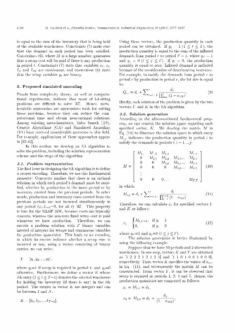
3.2. Solution generationAccording to the aforementioned fundamental prop-erty, we can restrict the solution space regarding eachspeci�ed vector, K. We develop the matrix M inEq. (10) to illustrate the solution space in which entryMi;j indicates the production quantity in period i tosatisfy the demands in periods i; i+ 1:::; j:

M =

266666664M1;1 M1;2 M1;3 M1;T

0 M2;1 M2;2 M2;3::: M2;T0 0 M3;3 M3;4::: M3;T0 0 0 M4;3::: M4;T...0 0 0 : : : MT;T

377777775 (10)

in which:

Mi;j = di +Xj

t=i+1

dtQt�1l=i (1� �ilk)

: (11)

Therefore, we can calculate xt for speci�ed vectors Yand K as follows:

xt =

(Mt;t0�1; if yt = 10; if yt = 0

(12)

where yt0=1 and yj=0 (t � j � t0).The solution generation is better illustrated by

using the following example.Suppose that we have 10 periods and 2 alternative

warehouses. In one step, vectors K and Y are obtainedas [1 2 2 2 1 2 1 2 1] and [1 1 0 1 0 0 1 0 0 0],respectively. Thus, vector K speci�es the values of �itkin Eq. (11), and subsequently the matrix M can beconstructed. From vector Y , it can be observed thatsetup is required in periods 1, 2, 4 and 7. Hence, theproduction quantities are computed as follows:

x1 = M1;1 = d1;

x2 = M2;3 = d2 +d3

(1� �222);


x4 =M4;6 =d4+d5

(1��442)+

d6

(1��442):(1��451);

x7 =M7;10(7; 10) = d7 +d8

(1� �771)

� d9

(1� �771):(1� �782)

+d10

(1� �771):(1� �782):(1� �791);

and:

x3 = x5 = x6 = x8 = x9 = x10 = 0:

3.3. Steps of the proposed solution based onSA

Using the above de�nitions and notation, the proposedalgorithm is developed as follows.

First, an initial solution should be determined. Kis a (T � 1)-tuple of random numbers between 1 to N .Y is a T -tuple of random binary numbers.

In the second step, a neighboring solution isconstructed. A random entry (i) of the vector K isselected, and its value is changed, where the new valueis also between 1 and N , randomly. Then, one period(j) is randomly selected, and the corresponding entryis switched from one to zero or zero to one in the vectorY . Notice that the �rst period should not be selected,because we assume that backlogging is not allowed inthe problem; in the �rst period, the setup must occuras well. At this time, using the obtained vectors Y andK, we exploit the lot sizes in each period according toEqs. (11) and (12), and then compute the �tness value.

This procedure is continued according to thesimulated annealing algorithm, and the pseudo-code ofthe proposed SA for the SILSP-MW is presented inFigure 1.

4. Computational study

In this section, we present a numerical example for fur-ther exposition of the problem and to further illustratethe proposed SA algorithm. Next, we compare the

Figure 1. Simulated annealing pseudo code for SILSP-MW.


performance of the proposed SA algorithm with thatof the heuristics proposed by Ho et al. [17], wherethe number of warehouses is equal to 1. Finally, anexperiment is designed to evaluate the performance ofthe SA algorithm, and to investigate the e�ect of theparameters on the SA algorithm.

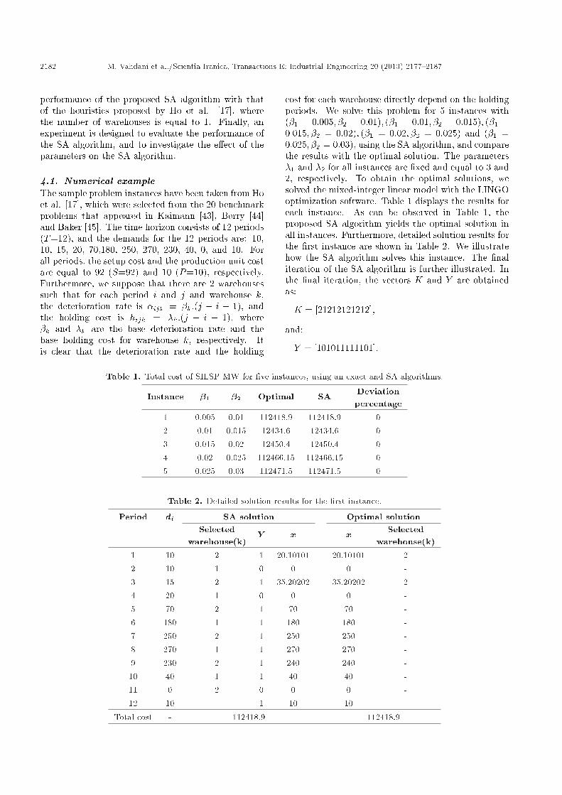
4.1. Numerical exampleThe sample problem instances have been taken from Hoet al. [17], which were selected from the 20 benchmarkproblems that appeared in Kaimann [43], Berry [44]and Baker [45]. The time horizon consists of 12 periods(T=12), and the demands for the 12 periods are: 10,10, 15, 20, 70,180, 250, 270, 230, 40, 0, and 10. Forall periods, the setup cost and the production unit costare equal to 92 (S=92) and 10 (P=10), respectively.Furthermore, we suppose that there are 2 warehousessuch that for each period i and j and warehouse k,the deterioration rate is �ijk = �k:(j � i + 1), andthe holding cost is hijk = �k:(j � i + 1), where�k and �k are the base deterioration rate and thebase holding cost for warehouse k, respectively. Itis clear that the deterioration rate and the holding

cost for each warehouse directly depend on the holdingperiods. We solve this problem for 5 instances with(�1 = 0:005; �2 = 0:01); (�1 = 0:01; �2 = 0:015); (�1 =0:015; �2 = 0:02); (�1 = 0:02; �2 = 0:025) and (�1 =0:025; �2 = 0:03), using the SA algorithm, and comparethe results with the optimal solution. The parameters�1 and �2 for all instances are �xed and equal to 3 and2, respectively. To obtain the optimal solutions, wesolved the mixed-integer linear model with the LINGOoptimization software. Table 1 displays the results foreach instance. As can be observed in Table 1, theproposed SA algorithm yields the optimal solution inall instances. Furthermore, detailed solution results forthe �rst instance are shown in Table 2. We illustratehow the SA algorithm solves this instance. The �naliteration of the SA algorithm is further illustrated. Inthe �nal iteration, the vectors K and Y are obtainedas:

K = [21212121212];

and:

Y = [101011111101]:

Table 1. Total cost of SILSP-MW for �ve instances, using an exact and SA algorithms.

Instance �1 �2 Optimal SA Deviationpercentage

1 0.005 0.01 112418.9 112418.9 02 0.01 0.015 12434.6 12434.6 03 0.015 0.02 12450.4 12450.4 04 0.02 0.025 112466.15 112466.15 05 0.025 0.03 112471.5 112471.5 0

Table 2. Detailed solution results for the �rst instance.

Period di SA solution Optimal solutionSelected

warehouse(k)Y x x Selected

warehouse(k)1 10 2 1 20.10101 20.10101 22 10 1 0 0 0 -3 15 2 1 35.20202 35.20202 24 20 1 0 0 0 -5 70 2 1 70 70 -6 180 1 1 180 180 -7 250 2 1 250 250 -8 270 1 1 270 270 -9 230 2 1 240 240 -10 40 1 1 40 40 -11 0 2 0 0 0 -12 10 - 1 10 10 -

Total cost - 112418.9 112418.9


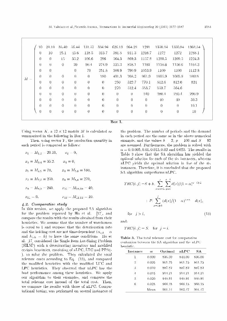
M =

0BBBBBBBBBBBBBBBBBBBBBBBB@

10 20:10 35:40 56:44 131:57 334:94 626:13 964:28 1291 1350:84 1350:84 1368:540 10 25:1 45:6 118:5 313:7 591:8 911:3 1216:7 1272 1272 1288:10 0 15 35:2 106:6 296 564:3 869:3 1157:8 1209:5 1209:5 1224:30 0 0 20 90:4 274:9 535:2 828:1 1102 1150:6 1150:6 1164:30 0 0 70 251:8 506:9 790:9 1053:9 1100 1100 1112:80 0 0 0 0 180 431:3 708:2 961:9 1005:9 1005:9 100180 0 0 0 0 0 250 522:7 770:1 812:6 812:6 8240 0 0 0 0 0 270 512:4 553:7 553:7 564:60 0 0 0 0 0 0 0 240 280:4 280:4 290:90 0 0 0 0 0 0 0 0 40 40 50:30 0 0 0 0 0 0 0 0 0 0 10:10 0 0 0 0 0 0 0 0 0 0 10

1CCCCCCCCCCCCCCCCCCCCCCCCABox I.

Using vector K, a 12 � 12 matrix M is calculated assummarized in the following in Box I.

Then, using vector Y , the production quantity ineach period is computed as follows:

x1 = M1;2 = 20:10; x2 = 0;

x3 = M3;4 = 35:2; x4 = 0;

x5 = M5;5 = 70; x6 = M6;6 = 180;

x7 = M7;7 = 250; x8 = M8;8 = 270;

x9 = M9;9 = 240; x10 = M10;10 = 40;

x11 = 0; x12 = M12;12 = 10:

4.2. Comparative studyIn this section, we apply the proposed SA algorithmfor the problem reported by Ho et al. [17], andcompare the results with the results obtained from theirheuristics. We assume that the number of warehousesis equal to 1 and suppose that the deterioration rateand the holding cost are not time-dependent (�ijk = �and hijk = h) to have the same conditions. Ho etal. [17] considered the Single Item Lot-Sizing Problem(SILSP) with a deteriorating inventory and modi�edcertain heuristics, consisting of nLPC, LTC and PPA(-), to solve the problem. They calculated the totalrelevant costs according to Eq. (13), and comparedthe modi�ed heuristics with the modi�ed LUC andLPC heuristics. They observed that nLPC has thebest performance among these heuristics. We applyour algorithm to their examples, and compute thetotal relevant cost instead of the total cost. Then,we compare the results with those of nLPC. Compu-tational testing was performed on several instances of

the problem. The number of periods and the demandin each period are the same as in the above numericalexample, and the values h = 2, p = 100 and S = 92are assumed. Furthermore, the problem is solved with� = 0; 0:005; 0:01; 0:015; 0:02 and 0:025. The results inTable 3 show that the SA algorithm has yielded theoptimal solution for each of the six instances, whereasnLPC yields the optimal solution in �ve of the sixinstances. Therefore, it is concluded that the proposedSA algorithm outperforms nLPC.

TRC(i; j) =S + h:jX

x=i+1

x�1Xy=i

d(x)=(1� �)y�i+1

+ P:jX

x=i+1

(d(x)=(1� �)x�i � d(x);

for j > i; (13)

and:

TRC(i; j) = S; for j = i:

Table 3. The total relevant cost for comparativeevaluation between the SA algorithm and the nLPCheuristic.

Instance � Optimal nLPC SA

1 0.000 836.00 844.00 836.002 0.005 861.75 861.75 861.753 0.010 887.82 887.82 887.824 0.015 914.21 914.21 914.215 0.020 940.91 940.91 940.916 0.025 966.15 966.15 966.15

Mean 901.14 902.47 901.47


4.3. An experimental design for additionalanalysis

An experiment was designed and performed for anoptimality sensitivity analysis of the proposed SA forsmall- and medium-sized problems. A full factorial ex-periment is conducted by varying the problem param-eters consisting of T (the number of periods), N (thenumber of warehouses), r (the ratio of the setup cost tothe base holding costs mean; that is S=(

PNi=1 �i=N)),

and ��(the mean of the base deterioration rate for thewarehouses.)In this analysis, the number of periodswas set at either of the two values: T = 10 and30. Demand in each period is generated by a discreteuniform distribution between 0 and 100; that is DU(0,100). The number of warehouses is also set at one ofthree values: N = 2; 5 and 10. The ratio r is set to oneof three values: 10, 40 and 100, and �� is set to one ofthree values: 0.003, 0.007 and 0.01. The problems with10 and 30 periods were considered small- and medium-sized problems, respectively. Table 4 shows the selectedparameters and their values. Combinations of thesefour parameters produced a total of 54 (2�3�3�3)experiments. Each experiment was repeated 10 times.The proposed SA algorithm was coded in the MATLABprogramming environment.

4.4. Computational resultsFor the designed experiments, the SA performancecan be analyzed by comparing the results with theoptimal solution. Tables 5 and 6 show the aver-age di�erences from the optimal solution for eachconducted experiment. On average, there is only a0.0314% di�erence from the optimum for small-sizedproblems, and the average di�erence from the optimumis 0.0786% for medium-sized problems. This veri�es thealgorithm performance. Notably, the optimal solutionwas obtained using the LINGO optimization package.

An analysis of variance (ANOVA) was used toidentify the parameters with a signi�cant e�ect on theperformance of the proposed SA algorithm. The resultsof the ANOVA at a 95% con�dence level are shownin Figure 2. As shown in Table 7, T (the number ofperiods), N (the number of warehouses) and r(the ratioof the setup cost to the mean base holding costs) havea signi�cant e�ect on the SA performance, whereas ��(the mean base deterioration rate for warehouses) hasno signi�cant e�ect.

Table 4. Selected parameters and their values for thedesigned experiment.

Parameters ValuesT 10, 30N 2, 5, 10R 10, 40, 100�� 0.003 '0.007 '0.01

Table 5. Computational results for small-sized (T = 10)problems

N r ��% Mean deviation

from optimum(gap)

2 10 0.003 00.007 00.01 0

40 0.003 00.007 00.01 0

100 0.003 00.007 0.00640.01 0.017

5 10 0.003 00.007 0.00310.01 0.0037

40 0.003 0.0270.007 0.00090.01 0.0067

100 0.003 0.0980.007 0.01020.01 0.08

10 10 0.003 0.0020.007 0.00140.01 0.0015

40 0.003 0.0270.007 0.0140.01 0.01

100 0.003 0.1730.007 0.1520.01 0.12

Mean 0.0314

Figure 2. Results of ANOVA at 95% con�dence level forselected parameters.

Furthermore, Figure 3 illustrates the e�ect of eachparameter on the percent di�erence from the optimum.

5. Conclusions

In this paper, we presented a mixed integer linearprogramming model for the single-item, single-level


Table 6. Computational results for medium-sized(T = 30) problems.

N r ��% Mean deviation

from optimum(gap)

2 10 0.003 00.007 00.01 0

40 0.003 0.00190.007 0.00240.01 0.0041

100 0.003 0.08350.007 0.06400.01 0.0656

5 10 0.003 0.02220.007 0.10890.01 0.0138

40 0.003 0.0360.007 0.03320.01 0.326

100 0.003 0.23250.007 0.10120.01 0.1962

10 10 0.003 0.00680.007 0.00320.01 0.0015

40 0.003 0.06810.007 0.05070.01 0.0439

100 0.003 0.36160.007 0.33040.01 0.2583

Mean 0.0786

Table 7. Signi�cant and insigni�cant parameters.

Parameters Responses(% deviation from optimum)

Tp

Np

rp

�� *p: Signi�cant parameter;

*: Insigni�cant parameter.

lot-sizing problem with a deteriorating inventory andmultiple warehouses. Because this problem can besolved optimally with exact solutions in a reasonabletime only for small-sized instances, an SA algorithmwas developed to solve the problem. The performanceof this algorithm was investigated in comparison with

Figure 3. Parameter e�ects on the % di�erence from theoptimum.

the optimal solution for small- and medium-sized prob-lems. The results con�rmed the improved performanceof the proposed Simulated Annealing algorithm. Inaddition, the e�ects of four parameters, T (the numberof periods), N (the number of warehouses), r (the ratioof the setup cost to the mean base holding costs) and� (the mean base deterioration rate for warehouses),on the SA performance, were investigated. For futureresearch, the model can be extended to a multi-levellot-sizing problem. It would also be interesting toconsider both a deteriorating inventory and disposalcosts in lot-sizing with multiple warehouses in MRPsystems.

References

1. Whitin, T.M., Theory of Inventory Management,Princeton University Press, Princeton, New Jersey, pp.62-72 (1957).

2. Ghare, P.N. and Schrader, G.F. \A model for expo-nentially decaying inventories", Journal of IndustrialEngineering, 14, pp. 238-243 (1963).

3. Tadikamalla, P.R. \An EOQ inventory model for itemswith gamma distributed deterioration", IIE Transac-tions, 10(1), pp. 100-103 (1978).

4. AL-Khedhairi, A. and Tadj, L. \Optimal control of aproduction inventory system with Weibull distributeddeterioration", Applied Mathmatical Science, 1 (35),pp.1703-1714 (2007).

5. Nahmias, S. and Wang, S. \A heuristic lot size reorderpoint model for decaying inventories", ManagementScience, 25 (1), pp. 90-97 (1979).

6. Hsu, P.H., Wee, H.M. and Teng, H.M. \Preservationtechnology investment for deteriorating inventory",International Journal of Production Economics, 124(2), pp. 338-394 (2010).

7. Shah, Y. \An order level lot size inventory model fordeteriorating items", IIE Transactions, 9 (1), pp. 108-112 (1977).


8. Cochen, M.A. \Joint pricing and ordering policiesfor exponentially decaying inventory with known de-mand", Naval Research Logistics Quarterly, 24(2), pp.257-268 (1977).

9. Dave, U. and Patel, L.K. \Policy inventory model fordeteriorating items with time proportional demand",Journal of the Operational Research Society, 32(11),pp. 137-142 (1981).

10. Kang, S. and Kim, I. \A study on the price and pro-duction level of the deteriorating inventory system",International Journal of Production Research, 21(6),pp. 899-908 (1983).

11. Wee, H.M. \A replenishment policy for items with aprice-dependent demand and a varying rate of dete-rioration", Production Planning & Control, 8(5), pp.494-499 (1997).

12. Nahmias, S. \Perishable inventory theory: A review",Operations Resarch, 30(4), pp. 680-708 (1982).

13. Raafat, F. \Survey of literature on continuously dete-riorating inventory model", Journal of the OperationalResearch Society, 42(1), pp. 27-37 (1991).

14. Goyal, S.K. and Giri, B.C. \Recent trends in model-ing of deteriorating inventory", European Journal ofOperational Research, 134 (1), pp. 1-16 (2001).

15. Bakker, M. Riezebos, J. and Teunter R.H. \Reviewof inventory systems with deterioration since 2001",European Journal of Operational Research, 221(2), pp.275-284 (2012).

16. Wee, H-M. and Shum, Y-S. \Model development fordeteriorating inventory in material requirement plan-ning systems", Computers and Industrial Engineering,36(1), pp. 219-225 (1999).

17. Ho, J.C., Solis, A.O. and Chang, Y.L. \An evaluationof lot-sizing heuristics for deteriorating inventory inmaterial requirements planning systems", Computers& Operation Research, 34(9), pp. 2562-2575 (2007).

18. Chu, L.Y. and Shen, Z.M. \Perishable stock lot-sizingproblem with modi�ed all-unit discount cost struc-tures", Global Supply Chain Management, TsinghuaUniversity Press, Beijing, pp. 13-18 (2002).

19. Hsu, V.N. \Dynamic economic lot size model withperishable inventory" , Management Science, 46(8),pp. 1159-1169 (2000).

20. Chu, L.Y., Hsu, V.N. and Shen Z-j.M. \An eco-nomic lot-sizing problem with perishable inventory andeconomies of scale costs: approximation and worst caseanalysis", Naval Reseasrch Logistics, 52(6), pp. 536-548 (2005).

21. Bai, Q., Xu, J. and Zhang Y. \An approximation solu-tion to the ELS model for perishable inventory withbacklogging", The 7th International Symposium onOperation Research and Its Applications (ISORA'08),pp. 66-73 (2008).

22. Pahl, J. and Vo�, S. \Discrete lot-sizing and schedulingincluding deterioration and perishability constraints",Advanced Manufacturing and Sustainable Logistics,

Lecture Notes in Business Information Processing.Springer Berlin Heidelberg, 46, pp. 345-357 (2010).

23. Pahl, J., Vo�, S. and Woodru�, D.L. \Discrete lot-sizing and scheduling with sequence dependent setuptimes and costs including deterioration and perisha-bility constraints", 44th International Conference onSystem Sciences, Hawaii, pp. 1-10 (2011).

24. Banerjee, S. and Agraval, S. \A two-warehouse in-ventory model for items with three-parameter Weibulldistribution deterioration, shortages and linear trendin demand", International Transactions in OperationalResearch, 15(6), pp. 755-775 (2008).

25. Chung, K.-J. and Huang T.S. \The optimal retailer'sordering policies for deteriorating items with limitedstorage capacity under trade credit �nancing", Inter-national Journal of Production Economics, 106(1), pp.127-145 (2007).

26. Dey, J. Mondal, S. and Maiti, M. \Two storageinventory problem with dynamic demand and intervalvalued lead-time over �nite time horizon under in a-tion and time-value of money", European Journal ofOperational Research, 185(1), pp. 170-194 (2008).

27. Dye, C.-Y., Ouyang, L.-Y. and Hsieh, T.-P. \Deter-ministic inventory model for deteriorating items withcapacity constraint and time-proportional backlog-ging rate", European Journal of Operational Research,178(3), pp. 789-807 (2007).

28. Hsieh, T.-P., Dye, C.-Y. and Ouyang, L.-Y. \Deter-mining optimal lot size for a two warehouse systemwith deterioration and shortages using net presentvalue", European Journal of Operational Research,191(1), pp. 182-192 (2008).

29. Jaggi, C.K., Khanna, A. and Verma P. \Two-warehouse partial backlogging inventory model fordeteriorating items with linear trend in demand un-der in ationary conditions", International Journal ofSystems Science, 42(7), pp. 1185-1196 (2011).

30. Lee, C.C. \Two-warehouse inventory model with de-terioration under FIFO dispatching policy", EuropeanJournal of Operational Research, 174(2), pp. 861-873(2006).

31. Lee, C. and Hsu, S. \A two-warehouse productionmodel for deteriorating inventory items with time-dependent demands", European Journal of OperationalResearch, 194(3), pp. 700-710 (2009).

32. Liao, J.-J. and Huang, K.-N. \Deterministic inventorymodel for deteriorating items with trade credit �nanc-ing and capacity constraints", Computers & IndustrialEngineering, 59(4), pp. 611-618 (2010).

33. Niu, B. and Xie, J. \A note on two-warehouse inven-tory model with deterioration under FIFO dispatchpolicy", European Journal of Operational Research,190(2), pp. 571-577 (2008).

34. Rong, M., Mahapatra, N.K. and Maiti, M. \A twowarehouse inventory model for a deteriorating itemwith partially/fully backlogged shortage and fuzzylead time", European Journal of Operational Research,189(1), pp. 59-75 (2008).


35. Yang, H.-L. \Two-warehouse inventory models fordeteriorating items with shortages under in ation",European Journal of Operational Research, 157(2), pp.344-356 (2004).

36. Yang, H.-L. \Two-warehouse partial backlogging in-ventory models for deteriorating items under in a-tion", International Journal of Production Economics,103 (1), pp. 362-370 (2006).

37. Jans, R. and Degraeve Z. \Meta-heuristics for dynamiclot sizing: A review and comparison of solution ap-proaches", European Journal of Operational Research,177(3), pp. 1855-1875 (2007).

38. Tang, O. \Simulated annealing in lot sizing problems",International Journal of Production Economics, 88(2),pp. 173-181 (2004).

39. Mishra. N., Kumar, V., Kumar, N., Kumar, M. andTiwari, M.K. \Addressing lot sizing and warehousingscheduling problem in manufacturing environment",Expert Systems with Applications, 38(9), pp. 11751-11762 (2011).

40. Mirabi, M. and Fatemi Ghomi, S.M.T. \A hybridsimulated annealing for the single machine capaci-tated lot-sizing and scheduling problem with sequence-dependent setup times and costs", Industrial Engi-neering and Engineering Management (IEEM), IEEEInternational Conference on Macao, 54, pp. 1261-1265(2010).

41. Lot�, G. \Applying genetic algorithms to dynamic lotsizing with batch ordering", Computers and IndustrialEngineering, 51(3), pp. 433-444 (2006).

42. Dellaert, N. Jeunet, J. and Jonard, N. \A genetic algo-rithm to solve the general multi-level lot-sizing prob-lem with time-varying costs", International Journal ofProduction Economics, 68(3) pp. 241-257 (2000).

43. Kiamann, R.A. \EOQ vs. dynamic programming-which one to use for invgentory ordering", Productionand Inventory Management, 10 (4), pp. 66-74 (1969).

44. Berry, W.L. \Lot sizing procedures for requirementsplanning systems: a framework for analysis", Pro-

duction and Inventory Management, 13(2), pp.19-34(1972).

45. Baker, K.R. \Lot-sizing procedures and a standarddata set: a reconciliation of the literature", Journalof Manufacturing and Operations Management, 2, pp.199-221 (1989).

Biographies

Mahmood Vahdani has been graduated in IndustrialEngineering in Shahed University. He received hisBS degree in Industrial Engineering from BojnourdUniversity in 2010 and his MS degree in IndustrialEngineering from Shahed University of Tehran in 2012.His research interests are production planning, perish-able inventories, lot-sizing problems and meta-heuristicalgorithms .

Ardeshir Dolati is Assistant Professor at ShahedUniversity. He received his BS degree in AppliedMathematics from Isfahan University of Technologyin 1997, and his MS and PhD degrees in AppliedMathematics from Amirkabir University of Technologyin 2000 and 2006, respectively. His research interestsare Network optimization, Combinatorial optimizationand Graph theory.

Mahdi Bashiri is Associate Professor at ShahedUniversity. He received his BS degree in IndustrialEngineering from Iran University of Science and Tech-nology in 1999, and his MS and PhD degrees inIndustrial Engineering from Tarbiat Modares Univer-sity of Tehran in 2001 and 2005, respectively. Hevisited the Statistics Department at London Schoolof Economics and Political Sciences in 2004 for sixmonths. His research interests are facility location andlayout, design of experiments and multiple responseoptimizations

Single-item lot-sizing and scheduling problem with ...

Documents

Transcript of Single-item lot-sizing and scheduling problem with ...