Single-Forward-Step Projective Splitting: ExploitingCocoercivity

Patrick R. Johnstone∗ Jonathan Eckstein∗

June 19, 2019

Abstract

This work describes a new variant of projective splitting for monotone inclusions,in which cocoercive operators can be processed with a single forward step per iteration.This result establishes a symmetry between projective splitting algorithms, the classi-cal forward-backward splitting method (FB), and Tseng’s forward-backward-forwardmethod (FBF). Another symmetry is that the new procedure allows for larger stepsizesfor cocoercive operators: the stepsize bound is 2β for a β-cocoercive operator, whichis the same as for FB. To complete the connection, we show that FB corresponds toan unattainable boundary case of the parameters in the new procedure. Unlike FB,the new method allows for a backtracking procedure when the cocoercivity constantis unknown. Proving convergence of the algorithm requires some departures from theusual proof framework for projective splitting. We close with some computational testsestablishing competitive performance for the method.

1 Introduction

For a collection of real Hilbert spaces {Hi}ni=0 consider the finite-sum convex minimizationproblem:

minx∈H0

n∑i=1

(fi(Gix) + hi(Gix)

), (1)

where every fi : Hi → (−∞,+∞] and hi : Hi → R is closed, proper, and convex, every hi isalso differentiable with Li-Lipschitz-continuous gradients, and the operators Gi : H0 → Hi

are linear and bounded. Under appropriate constraint qualifications, (1) is equivalent to themonotone inclusion problem of finding z ∈ H0 such that

0 ∈n∑i=1

G∗i (Ai +Bi)Giz (2)

∗Department of Management Science and Information Systems, Rutgers Business School Newark and NewBrunswick, Rutgers University. Contact: patrick.r.johnstone@gmail.com, jeckstei@business.rutgers.edu

1

where all Ai : Hi → 2Hi and Bi : Hi → Hi are maximal monotone and each Bi is L−1i -cocoercive, meaning that it is single-valued and

Li〈Bix1 −Bix2, x1 − x2〉 ≥ ‖Bix1 −Bix2‖2

for some Li ≥ 0. In particular, if we set Ai = ∂fi and Bi = ∇hi then the solution sets of thetwo problems coincide under a special case of the constraint qualification of [9, Prop. 5.3].When Li = 0, then Bi must be a constant operator, that is, there is some vi ∈ Hi such thatBix = vi for all x ∈ Hi. Defining Ti = Ai +Bi, problem (2) may be written more compactlyas

0 ∈n∑i=1

G∗iTiGiz. (3)

1.1 Background

Operator splitting algorithms are an effective way to solve structured convex optimizationproblems and monotone inclusions such as (1), (2), and (3). Their defining feature is thatthey break the problem up into managable chunks. At each iteration they solve a set oftractable subproblems in such a manner as to converge to a solution of the global problem.Arguably the three most popular operator splitting algorithms are the forward-backwardsplitting (FB) [11], Douglas/Peaceman-Rachford splitting (DR) [24], and forward-backward-forward (FBF) [38] methods. Indeed, many algorithms in convex optimization and monotoneinclusions are in fact instances of one of these methods.

A different and relatively recently proposed class of operator splitting algorithms is pro-jective splitting. Projective splitting has a different convergence analysis from most opera-tor splitting schemes: while the convergence of most schemes is obtained by viewing theirupdates as a fixed-point iteration, often of some firmly non-expansive operator, projectivesplitting is analyzed (and designed) as a way of creating a sequence of separating hyperplanesbetween the current iterate and the primal-dual solution set. New iterates are produced byprojecting onto these hyperplanes, perhaps with some over- or under-relaxation. The classof methods originated in [18], was extended to sums of n ≥ 1 operators in [19], to includecompositions with bounded linear maps in [1], to allow asynchronous block-iterative (i.e. in-cremental) updates in [10], and to allow forward steps for Lipschitz continuous operators in[37, 21]. Further theoretical results, including some convergence rates, have been obtainedin [20, 22, 27, 26].

In the context of projective splitting, [37, 21] were the first works to move away fromcomputational updates based solely on resolvent steps on each maximal monotone operatorTi in (3). The analysis in [21] developed a procedure that could instead use two forward(explicit or gradient) steps for Lipschitz continuous operators. This innovation constitutedsignificant progress because forward steps are often computationally much cheaper and moreconvenient than resolvents. However, the result raised a question: if projective splittingcan exploit Lipschitz continuity, can it further exploit the presence of cocoercive operators?Cocoercivity is in general a stronger property than Lipschitz continuity. However, when anoperator is the gradient of a closed proper convex function (such as hi in (1)), the Baillon-Haddad theorem [2, 3] establishes that the two properties are equivalent: ∇hi is Li-Lipschitzcontinuous if and only if it is L−1i -cocoercive.

2

Operator splitting methods that exploit cocoercivity rather than mere Lipschitz con-tinuity typically have lower per-iteration computational complexity and a larger range ofpermissible stepsizes. For example, both FBF and the extragradient (EG) method [23]only require Lipchitz continuity, but need two forward steps per iteration and limit thestepsize to L−1, where L is the Lipschitz constant. If we strengthen the assumption to L−1-cocoercivity, we can use FB, which only needs one forward step per iteration and allowsstepsizes bounded away from 2L−1. One departure from this pattern is the recently devel-oped method of [29], which only requires Lipschitz continuity but uses just one forward stepper iteration. While this property is remarkable, it should be noted that its stepsizes mustbe bounded by (1/2)L−1, which is half the allowable stepsize for EG or FBF.

Much like FBF and EG, the projective splitting computation in [21] requires Lipschitzcontinuity1, two forward steps per iteration, and limits the stepsize to be less than L−1

(when not using backtracking). Considering the relationship between FB and FBF/EGleads to following question: is there a variant of projective splitting which converges underthe stronger assumption of L−1-cocoercivity, while processing each cocoercive operator witha single forward step per iteration, allowing stepsizes bounded above by 2L−1?

In this paper, we answer this question in the affirmitive. Referring to (2), the newprocedure requires one forward step on Bi and one resolvent for Ai at each iteration. Whenthe resolvent is easily computable (for example, when Ai is the zero map and its resolventis simply the identity), the new procedure can effectively halve the computation necessaryto run the same number of iterations as the previous procedure of [21]. This advantage isequivalent to that of FB over FBF and EG when cocoercivity is present. Another advantageof the proposed method is that it allows for a backtracking linesearch when the cocoercivityconstant is unknown, whereas no such variant is currently known for FB.

The analysis of this new method is significantly different from our previous work in [21],using a novel “ascent lemma” (Lemma 16) regarding the separating hyperplanes generatedby the algorithm. The new procedure has an interesting connection to the original resolventcalculation used in the projective splitting papers [18, 19, 1, 10]: in Section 2.2 below, weshow that the new procedure is equivalent to one iteration of FB applied to evaluating theresolvent of Ti = Ai+Bi. That is, we can use a single forward-backward step to approximatethe operator-processing procedure in [18, 19, 1, 10], but still obtain convergence.

The new procedure has significant potential for asynchronous and incremental implemen-tation following the ideas and techniques of previous projective splitting methods [10, 17, 21].To keep the analysis managable, however, we plan to develop such generalizations in a follow-up paper. Here, we will simply assume that every operator is processed once per iteration.

1.2 The Optimization Context

Due to its importance in many applications, we give a brief discussion of the significance ofthe proposed method in the optimization context, i.e. solving (1). For this problem, the newmethod is a first-order proximal splitting method which fully splits the problem: it utilizesthe proximal operator for each nonsmooth function fi, a single gradient ∇hi for each smooth

1If backtracking is used then all three of these methods can converge under weaker local continuityassumptions.

3

function hi, and matrix multiplications by Gi and G∗i (not matrix inversions). Beyond these,the only computations at each iteration are a constant number of inner products, norms,scalar multiplications, and vector additions, which can all be carried out with flop countslinear in the dimension of each Hilbert space.

There are a few other first-order proximal splitting methods which can achieve full split-ting on (2). The most similar to projective splitting are those in the family of primal-dual(PD) splitting methods; see [13, 12, 7, 33] and references therein. In fact, projective split-ting is also a kind of primal-dual method, since it produces a primal sequence and a dualsequence both converging to a primal-dual solution. However, the convergence mechanismsare entirely different: PD methods are usually built by applying an established operatorsplitting technique such as FB, FBF, or DR to the appropriately formulated primal-dualinclusion in a primal-dual product space.

Apart from being new, we list two potential advantages of our proposed method over themore established PD schemes. First, unlike the PD methods, the norms ‖Gi‖ do not effectthe stepsize constraints of our proposed method, making such constraints easier to satisfy.Furthermore, differently from PD methods, the stepsizes may vary at each iteration and maydiffer for each operator. Second, projective splitting methods allow for asynchronous paralleland incremental implementations in an arguably simpler way than PD methods (althoughwe do not develop this aspect in this paper). In projective splitting it is fairly straight-forward to incorporate deterministic asynchronous assumptions [10, 17] with deterministicconvergence guarantees, with the analysis being similar to the synchronous case. In contrast,existing asynchronous and block-coordinate analyses of PD methods have required stochasticassumptions which only lead to probabilistic convergence guarantees [33].

1.3 Notation and a Simplifying Assumption

We use the same general notation as in [21, 20, 22]. Summations of the form∑n−1

i=1 ai willappear throughout this paper. To deal with the case n = 1, we use the standard conventionthat

∑0i=1 ai = 0.

We will use a boldface w = (w1, . . . , wn−1) for elements of H1 × . . . × Hn−1. Let H ,H0 × H1 × · · · × Hn−1, which we refer to as the “collective primal-dual space”, and notethat the assumption on Gn implies that Hn = H0. We use p to refer to points in H, sop , (z,w) = (z, w1, . . . , wn−1).

Throughout, we will simply write ‖ · ‖i = ‖ · ‖ as the norm for Hi and let the subscriptbe inferred from the argument. In the same way, we will write 〈·, ·〉i as 〈·, ·〉 for the innerproduct of Hi. For the collective primal-dual space we will use a special norm and innerproduct with its own subscript defined in (15).

We use the standard “⇀” notation to denote weak convergence, which is of course equiv-alent to ordinary convergence in finite-dimensional settings.

For any maximal monotone operator A we will use the notation JρA , (I + ρA)−1, forany scalar ρ > 0, to denote the resolvent operator, also known as the proximal, backward,or implicit step with respect to A. Thus,

x = JρA(t) ⇐⇒ x+ ρa = t and a ∈ Ax, (4)

4

and the x and a satisfying this relation are unique. Furthermore, JρA is defined everywhereand range(JA) = dom(A) [4, Prop. 23.2].

For the rest of the paper, we will impose the simplifying assumption

Gn : Hn → Hn , I (the identity operator).

As noted in [21], the requirement that Gn = I is not a very restrictive assumption. Forexample, one can always enlarge the original problem by one operator, setting An = Bn = 0.

2 Projective Splitting

The goal of our algorithm will be to find a point in

S ,{

(z, w1, . . . , wn−1) ∈H∣∣ (∀ i ∈ {1, . . . , n− 1}) wi ∈ TiGiz, −

∑n−1i=1 G

∗iwi ∈ Tnz

}.(5)

It is clear that z∗ solves (2)–(3) if and only if there exist w∗1, . . . , w∗n−1 such that

(z∗, w∗1, . . . , w∗n−1) ∈ S.

Under reasonable assumptions, the set S is closed and convex; see Lemma 1. S is oftencalled the Kuhn-Tucker solution set of problem (3).

A separator-projector algorithm for finding a point in S (and hence a solution to (3))will, at each iteration k, find a closed and convex set Hk which separates S from the currentpoint, meaning S is entirely in the set (preferably, the current point is not). One can thenattempt to “move closer” to the solution set by projecting the current point onto the setHk. This general setup guarantees that the sequence generated by the method is Fejermonotone [8] with respect to S. This alone is not sufficient to guarantee that the iteratesactually converge to a point in the solution set. To establish this, one needs to show thatthe set Hk “sufficiently separates” the current point from the solution set, or at least doesso sufficiently often. Such “sufficient separation” allows one to establish that any weaklyconvergent subsequence of the iterates must have its limit in the set S, from which overallweak convergence follows from [8, Prop. 2].

With S as in (5), the separator formulation presented in [10] constructs the halfspace Hk

using the function

ϕk(z, w1, . . . , wn−1) ,n−1∑i=1

〈Giz − xki , yki − wi〉+

⟨z − xni , yni +

n−1∑i=1

G∗iwi

⟩(6)

=

⟨z,

n∑i=1

G∗i yki

⟩+

n−1∑i=1

〈xki −Gixkn, wi〉 −

n∑i=1

〈xki , yki 〉, (7)

for some (xki , yki ) ∈ H2

i such that yki ∈ Tixki , i ∈ 1, . . . , n. These points (xki , y

ki ) will be

specified later and must be updated in a specific way in order to guarantee convergence to S.From its expression in (7) it is clear that ϕk is an affine function on H. Furthermore, from (6)it may easily be verified using the monotonicity of each Ti that for any p = (z, w1, . . . , wn−1) ∈

5

S, one has ϕk(p) ≤ 0, so that the separator set Hk may be taken to be the halfspace{p | ϕk(p) ≤ 0}. Projecting onto this halfspace is a low-complexity operation involvingonly inner products, norms, matrix multiplication by Gi, and sums of scalars. For example,when Hi = Rd for i = 1, . . . , n and each Gi = I, then this projection has computationalcomplexity O(nd).

The key question is how to select the points (xki , yki ) ∈ gra Ti so that convergence to S may

be established. The original approach, given the current iterate pk = (zk, wk1 , . . . , wkn−1), is to

choose (xki , yki ) ∈ gra Ti to be some function of (zk, wki ) such that ϕk(p

k) is positive and “suffi-ciently large” whenever pk 6∈ S. Then, since the solution set is entirely on the nonpositive sideof the hyperplane {p | ϕk(p) = 0}, projecting the current point onto this hyperplane makesprogress toward the solution and can be shown to lead to overall convergence. In the originalversions of projective splitting, the calculation of (xki , y

ki ) involved (perhaps approximately)

evaluating a resolvent; [21] introduced the alternative of a two-forward-step calculation forLipschitz continuous operators. Here, we introduce a one-forward-step calculation for thecase of cocoercive operators

A principal difference between the analysis here and earlier work on projective splittingis that processing all the operators T1, . . . , Tn at iteration k need not result in ϕk(p

k) be-ing positive. Instead, we establish an “ascent lemma” that relates the values ϕk(p

k) andϕk−1(p

k−1) in such a way that overall convergence may still be proved, even though it is pos-sible that ϕk(p

k) ≤ 0. When ϕk(pk) ≤ 0, projection onto Hk = {p | ϕk(p) ≤ 0} is effectively

a “no-operation” resulting in pk+1 = pk. In this case, the algorithm continues to computenew points (xk+1

i , yk+1i ), (xk+2

i , yk+2i ), . . . until, for some ` ≥ 0, it constructs a hyperplane

Hk+` such that the ϕk+`(pk) > 0 and projection results in pk+`+1 6= pk+` = pk.

Additional Notation for Projective Splitting

For an arbitrary (w1, w2, . . . , wn−1) ∈ H1 ×H2 × . . .×Hn−1 we use the notation

wn , −n−1∑i=1

G∗iwi.

Note that when n = 1, w1 = 0. Under this convention, we may write ϕk : H → R in thesimpler form

ϕk(z, w1, . . . , wn−1) =n∑i=1

〈Giz − xki , yki − wi〉.

We also use the following notation for i = 1, . . . , n:

ϕi,k(z, wi) , 〈Giz − xki , yki − wi〉.

Note that ϕk(p) = ϕk(z, w1, . . . , wn−1) =∑n

i=1 ϕi,k(z, wi).

6

2.1 The New Procedure

Suppose Ai = 0 for some i ∈ {1, . . . , n}. Since Bi is cocoercive, it is also Lipschitz continuous.In [21] we introduced the following two-forward-step update for Lipschitz continuous Bi:

xki = Gizk − ρki (BiGiz

k − wki )yki = Bix

ki .

Under Li-Lipschitz continuity and the condition ρki < 1/Li, it is possible to show thatupdating (xki , y

ki ) in this way leads to ϕi,k(z

k, wki ) being sufficiently positive to establishoverall convergence. Although we did not discuss it in [21], this two-forward step procedurecan be extended to handle nonzero Ai in the following manner:

xki + ρki aki = Giz

k − ρki (BiGizk − wki ) : aki ∈ Aixki (8)

yki = aki +Bixki . (9)

Following (4), it is clear that (8) is essentially a resolvent calculation applied to its right-handside Giz

k − ρki (BiGizk − wki ). This type of update, with forward steps and backward steps

together, was introduced in [37] for a more limited form of projective splitting.An obvious drawback of (8)–(9) is that it requires two forward steps per iteration, one to

compute BiGizk and another to compute Bix

ki . The initial motivation for the current paper

was the following question: is there a way to reuse Bixk−1i so as to avoid computing BiGiz

k

at each iteration, perhaps under the stronger assumption of cocoercivity? With some effortwe arrived at the following update for each block i = 1, . . . , n at each iteration k ≥ 0:

xki + ρki aki = (1− αki )xk−1i + αkiGiz

k − ρki(bk−1i − wki

): aki ∈ Aixki (10)

bki = Bixki (11)

yki = aki + bki , (12)

where αki ∈ (0, 1), ρki ≤ 2(1 − αki )/Li, and b0i = Bix0i . Condition (10) is readily satisfied

by some simple linear algebra calculations followed by a resolvent calculation involving Ai.Subsequently, (11) requires only an evaluation (forward step) on Bi, and (12) is a simplevector addition. In comparison to (8), we have replaced BiGiz

k with the previously computedpoint Bix

k−1i . However, in order to establish convergence, it turns out that we also need to

replace Gizk with a convex combination of xk−1i and Giz

k. Note that the stepsize constraintcan now be made arbitrarily close to 2/Li by setting αki arbitrarily close to 0. However, inpractice it may be better to use an intermediate value, such as αki = 0.1, since this allowsthe update to make significant use of the information in zk, a point computed more recentlythan xk−1i .

Computing (xki , yki ) in this way does not guarantee that ϕi,k(z

k, wki ) is positive. In thenext section, we give some intuition as to why (10)-(12) nevertheless leads to convergenceto S.

2.2 A Connection with the Forward-Backward Method

In the projective splitting literature preceeding [21], the pairs (xki , yki ) are solutions of

xki + ρki yki = Giz

k + ρkiwki : yki ∈ Tixki (13)

7

for some ρki > 0, which — following (4) — is a resolvent calculation. It can be shown thatthe resulting (xki , y

ki ) ∈ gra Ti are such that ϕi,k(z

k, wki ) is positive and sufficiently large toguarantee overall convergence to a solution of (3). Since the stepsize ρki in (13) can be anypositive number, let us replace ρki with ρki /α

ki for some αki ∈ (0, 1) and rewrite (13) as

xki +ρkiαkiyki = Giz

k +ρkiαkiwki : yki ∈ Tixki . (14)

The reason for this reparameterization will become apparent below.In this paper, Ti = Ai +Bi, with Bi being cocoercive and Ai maximal monotone. For Ti

in this form, computing the resolvent as in (13) exactly may be impossible, even when theresolvent of Ai is available. With this structure, xki in (14) satisfies:

0 ∈ ρkiαkiAix

ki +

ρkiαkiBix

ki + xki −

(Giz

k +ρkiαkiwki

)which can be rearranged to 0 ∈ Aixki + Bix

ki , where

Biv = Biv +αkiρki

(v −Giz

k − ρkiαkiwki

).

Since Bi is L−1i -cocoercive, Bi is (Li + αki /ρki )−1-cocoercive [4, Prop. 4.12]. Consider the

generic monotone inclusion problem 0 ∈ Aix + Bix: Ai is maximal and Bi is cocoercive,and thus one may solve the problem with the forward-backward (FB) method [4, Theorem26.14]. If one applies a single iteration of FB initialized at xk−1i , with stepsize ρki , to theinclusion 0 ∈ Aix+ Bix, one obtains the calculation:

xki = Jρki Ai

(xk−1i − ρki Bix

k−1i

)= Jρki Ai

(xk−1i − ρki

(Bix

k−1i +

αkiρki

(xk−1i −Giz

k − ρkiαkiwki

)))= Jρki Ai

((1− αki )xk−1i + αkiGiz

k − ρki(Bix

k−1i − wki

)),

which is precisely the update (10). So, our proposed calculation is equivalent to one iterationof FB initialized at the previous point xk−1i , applied to the subproblem of computing theresolvent in (14). Prior versions of projective splitting require computing this resolvent eitherexactly or to within a certain relative error criterion, which may be costly. Here, we simplymake a single FB step toward computing the resolvent, which we will prove is sufficient forthe projective splitting method to converge to S. However, our stepsize restriction on ρkiwill be slightly stronger than the natural stepsize limit that would arise when applying FBto 0 ∈ Aix+ Bix

3 The Algorithm: Assumptions, Definition, and Basic

Properties

Assumption 1. Problem (2) conforms to the following:

8

1. H0 = Hn and H1, . . . ,Hn−1 are real Hilbert spaces.

2. For i = 1, . . . , n, the operators Ai : Hi → 2Hi and Bi : Hi → Hi are monotone.Additionally each Ai is maximal.

3. Each operator Bi is either L−1i -cocoercive for some Li > 0 (and thus single-valued) anddomBi = Hi, or Li = 0 and Bix = vi for all x ∈ Hi and some vi ∈ Hi.

4. Each Gi : H0 → Hi for i = 1, . . . , n− 1 is linear and bounded.

5. Problem (2) has a solution, so the set S defined in (5) is nonempty.

In order to apply a separator-projector algorithm, the target set must be closed andconvex. Establishing this for S is very similar to in our previous work [21], which in turnfollows many earlier results.

Lemma 1. Suppose Assumption 1 holds. The set S defined in (5) is closed and convex.

Proof. By [4, Cor. 20.28] each Bi is maximal. Furthermore, since dom(Bi) = Hi, Ti = Ai+Bi

is maximal monotone by [4, Cor. 25.5(i)]. The rest of the proof is identical to [21, Lemma3].

Throughout, we will use p = (z,w) = (z, w1, . . . , wn−1) for a generic point in H, thecollective primal-dual space. For H, we adopt the following (standard) norm and innerproduct:

‖(z,w)‖2 , ‖z‖2 +n−1∑i=1

‖wi‖2⟨(z1,w1), (z2,w2)

⟩, 〈z1, z2〉+

n−1∑i=1

〈w1i , w

2i 〉. (15)

Lemma 2. [21, Lemma 4] Let ϕk be defined as in (6). Then:

1. ϕk is affine on H.

2. With respect to inner product 〈·, ·〉 on H, the gradient of ϕk is

∇ϕk =

(n−1∑i=1

G∗i yki + ykn, x

k1 −G1x

kn, x

k2 −G2x

kn, . . . , x

kn−1 −Gn−1x

kn

).

We sharpen the notation for the one-forward-step update introduced in (10)–(12) asfollows:

Definition 1. Suppose H and H′ are real Hilbert spaces, A : H → 2H is maximal-monotonewith nonempty domain, B : H → H is L−1-cocoercive, and G : H′ → H is bounded andlinear. For α ∈ [0, 1] and ρ > 0, define the mapping Fα,ρ(z, x, w;A,B,G) : H′ ×H2 → H2,with additional parameters A,B, and G, as

Fα,ρ

(z, x, w;

A,B,G

): = (x+, y+) :

t , (1− α)x+ αGz − ρ(Bx− w)

x+ = JρA (t)

y+ = ρ−1(t− x+) +Bx+.

(16)

9

Algorithm 1: One-Forward-Step Projective Splitting with Backtracking

Input: (z1,w1) ∈H, {βk}k∈N, B ⊆ {1, . . . , n} the operators requiring backtracking,γ > 0, δ ∈ (0, 1). For i = 1, . . . , n: x0i ∈ Hi and {αki }k∈N. For i ∈ B: {ρki }k∈N,θi ∈ dom(Ai), wi ∈ Aiθi +Biθi, and y0i ∈ Aix0i +Bix

0i . For i /∈ B: {ρki }k∈N.

1 for k = 1, 2, . . . do2 for i ∈ B do3 ϕi,k−1(z

k, wki )← 〈Gizk − xk−1i , yk−1i − wki 〉

4 (xki , yki , ρ

ki )← backTrack(zk, wki , xk−1i , yk−1i , ρki , ϕi,k−1(z

k, wki ), αki , θi, wi, δ;Ai, Bi, Gi)

5 for i /∈ B do6 (xki , y

ki )← Fαk

i ,ρki(zk, xk−1i , wki ;Ai, Bi, Gi) /* F defined in (16) */

7 (πk, zk+1,wk+1) ← projectToHplane(zk, wk, {xki , yki }ni=1, βk, γ)

8 if πk = 0 then9 return zk+1

Algorithm 2: Backtracking procedure

1 Function backTrack(z, w, x, y, ρ, ϕ, α, θ, w, δ; A, B, G):2 ρ1 = ρ3 for j = 1, 2, . . . do4 (xj, yj) = Fα,ρj(z, x, w;A,B,G) /* F defined in (16) */

5 yj = ρ−1j ((1− α)x+ αGz − xj) + w

6 ϕ+j = 〈Gz − xj, yj − w〉

7 if ‖xj − θ‖ ≤ (1− α)‖x− θ‖+ α‖Gz − θ‖+ ρj‖w − w‖8 and ϕ+

j ≥ρj2α

(‖yj − w‖2 + α‖yj − w‖2) + (1− α)(ϕ− ρj

2α‖y − w‖2

)then

9 return (xj, yj, ρj)

10 ρj+1 = δρj

With this notation, (10)–(12) can be written as

(xki , yki ) = Fαk

i ,ρki(zk, xk−1i , wki ;Ai, Bi, Gi).

Algorithms 1–3 define the main method proposed in this work. They produce a sequenceof primal-dual iterates pk = (zk, wk1 , . . . , w

kn−1) ∈ H and, implicitly, wkn , −

∑n−1i=1 G

∗iw

ki .

Algorithm 1 gives the basic outline of our method; for each operator, it invokes either ournew one-forward-step update with a user-defined stepsize (through line 6) or its backtrackingvariant given in Algorithm 2 (through line 4). Together, algorithms 1–2 specify how to updatethe points (xki , y

ki ) used to define the separating affine function ϕk in (6). Algorithm 3,

called from line 7 of Algorithm 1, defines the projectToHplane function that performs theprojection step to obtain the next iterate.

Taken together, algorithms 1–3 are essentially the same as Algorithm 2 of [21], exceptthat the update of (xki , y

ki ) uses the new procedure given in (10)–(12). For simplicity, the

10

Algorithm 3: Projection Update

Global Variables for Function: Gi : H0 → Hi for i = 1, . . . , n− 11 Function projectToHplane(z,w, {xi, yi}ni=1, β, γ):2 ui = xi −Gixn, i = 1, . . . , n− 1,

3 v =∑n−1

i=1 G∗i yi + yn

4 π = ‖u‖2 + γ−1‖v‖25 if π > 0 then

6 ϕ(p) = 〈z, v〉+∑n−1

i=1 〈wi, ui〉 −∑n

i=1〈xi, yi〉7 τ = β

πmax {0, ϕ(p)}

8 else9 return (0, xn, y1, . . . , yn−1)

10 z+ = z − γ−1τv11 w+

i = wi − τui, i = 1, . . . , n− 1,

12 w+n = −

∑n−1i=1 G

∗iw

+i

13 return (π, z+,w+)

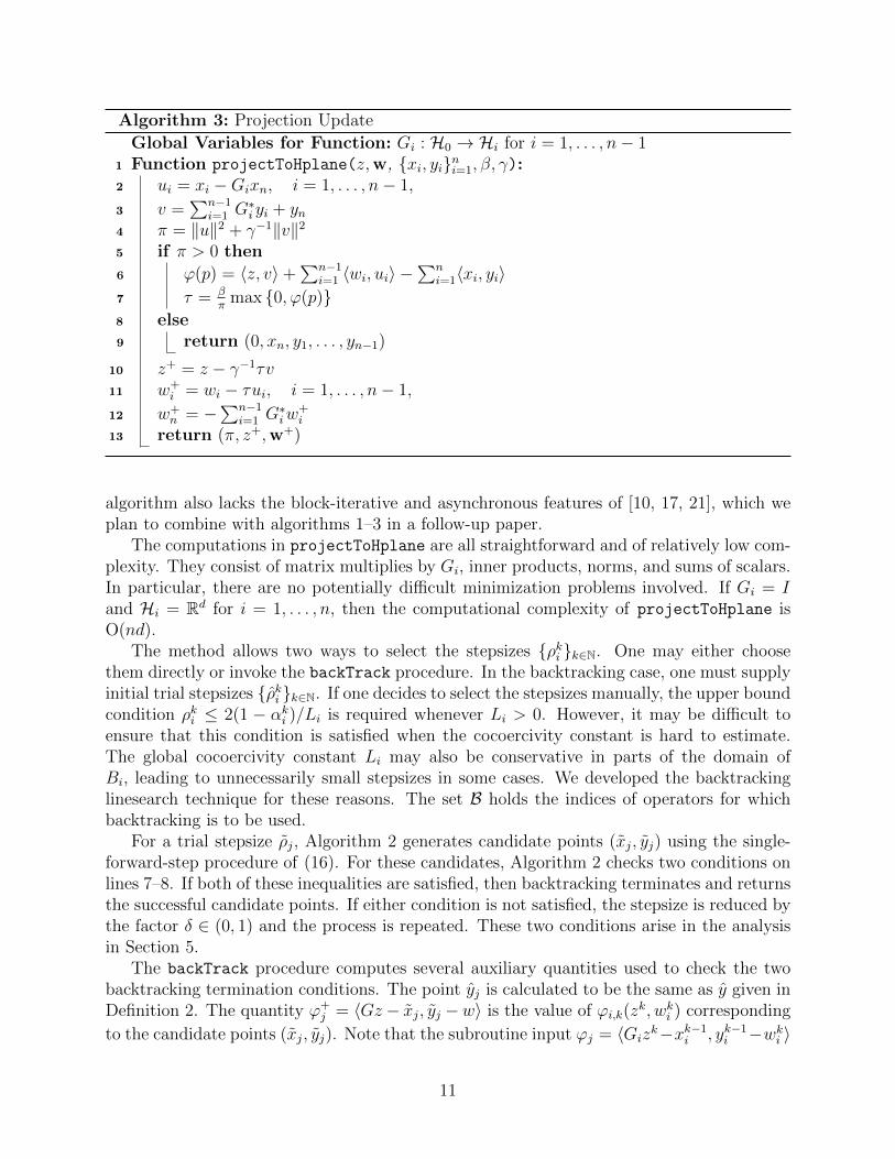
algorithm also lacks the block-iterative and asynchronous features of [10, 17, 21], which weplan to combine with algorithms 1–3 in a follow-up paper.

The computations in projectToHplane are all straightforward and of relatively low com-plexity. They consist of matrix multiplies by Gi, inner products, norms, and sums of scalars.In particular, there are no potentially difficult minimization problems involved. If Gi = Iand Hi = Rd for i = 1, . . . , n, then the computational complexity of projectToHplane isO(nd).

The method allows two ways to select the stepsizes {ρki }k∈N. One may either choosethem directly or invoke the backTrack procedure. In the backtracking case, one must supplyinitial trial stepsizes {ρki }k∈N. If one decides to select the stepsizes manually, the upper boundcondition ρki ≤ 2(1 − αki )/Li is required whenever Li > 0. However, it may be difficult toensure that this condition is satisfied when the cocoercivity constant is hard to estimate.The global cocoercivity constant Li may also be conservative in parts of the domain ofBi, leading to unnecessarily small stepsizes in some cases. We developed the backtrackinglinesearch technique for these reasons. The set B holds the indices of operators for whichbacktracking is to be used.

For a trial stepsize ρj, Algorithm 2 generates candidate points (xj, yj) using the single-forward-step procedure of (16). For these candidates, Algorithm 2 checks two conditions onlines 7–8. If both of these inequalities are satisfied, then backtracking terminates and returnsthe successful candidate points. If either condition is not satisfied, the stepsize is reduced bythe factor δ ∈ (0, 1) and the process is repeated. These two conditions arise in the analysisin Section 5.

The backTrack procedure computes several auxiliary quantities used to check the twobacktracking termination conditions. The point yj is calculated to be the same as y given inDefinition 2. The quantity ϕ+

j = 〈Gz − xj, yj −w〉 is the value of ϕi,k(zk, wki ) corresponding

to the candidate points (xj, yj). Note that the subroutine input ϕj = 〈Gizk−xk−1i , yk−1i −wki 〉

11

is equal to ϕi,k−1(zk, wki ). Ideally, we want ϕ+

j to be as large as possible, but the conditionchecked on line 8 will ultimately suffice to prove convergence.

Algorithm 1 has the following parameters. Precise assumptions regarding these parame-ters are given at the end of this section and in Section 5.5.

{αki }k∈N: as described in Section 2.2.

{ρki }k∈N: Note that ρki has two meanings. For i /∈ B, it is the user-supplied stepsize. Fori ∈ B, it is the stepsize returned by backTrack on line 4.

{ρki }k∈N: the initial trial stepsizes for the backtracking procedure for i ∈ B.

(θi, wi) these are used in the backtracking procedure for i ∈ B. An obvious choice whichwe used in our numerical experiments was (θi, wi) = (x0i , y

0i ), i.e. the initial point.

{βk}k∈N: relaxation factors for the projection operation.

γ > 0: allows for the projection to be performed using a slightly more general primal-dualmetric than (15). In effect, this parameter changes the relative size of the primal anddual updates in lines 10–11 of Algorithm 3. As γ increases, a smaller step is taken inthe primal and a larger step in the dual. As γ decreases, a smaller step is taken inthe dual update and a larger step is taken in the primal. See [19, Sec. 5.1] and [18,Sec. 4.1] for more details.

As written, Algorithm 1 is not as efficient as it could be. On the surface, it seems thatwe need to recompute Bix

k−1i in order to evaluate F on line 6. However, Bix

k−1i was already

computed in the previous iteration and can obviously be reused, so only one evaluation ofBi is needed per iteration. Similarly, within backTrack, each invocation of F on line 4 mayreuse the quantity Bx = Bix

k−1i which was computed in the previous iteration of Algorithm

1. Thus, each iteration of the loop within backTrack requires one new evaluation of B, tocompute Bxj within F .

Finally, we note that ρki is returned by backTrack only to make the notation within theproofs more streamlined. With this notation, assuming that backTrack always terminatesfinitely (which we will show to be the case), we may write

(xki , yki ) = Fαk

i , ρki(zk, xk−1i , wki ;Ai, Bi, Gi)

for all i = 1, . . . , n. The only difference between i ∈ B and i /∈ B is that in the former, thestepsize ρki is discovered by backtracking, while in the latter it is directly user-supplied.

We now list most of our parameter assumptions; however, one additional assumption isintroduced in Section 5.5, where it arises in the analysis.

Assumption 2. There exist 0 < β ≤ β < 2 such that β ≤ βk ≤ β for all k ≥ 1. Theconstant γ is positive. The constant δ ∈ (0, 1).

Assumption 3. For all i = 1, . . . , n there exists 0 < αi ≤ αi ≤ 1 such that αi ≤ αki ≤ αifor all k ≥ 1. There exists cα ∈ (0, 1) such that for all k ≥ 1 and i = 1, . . . , n,

αki ≤cαα

k−1i

1− αk−1i

. (17)

12

Assumption 4. For i /∈ B and for all k ≥ 1:

1. There exists ρi

such that 0 < ρi≤ ρki .

2. If Li = 0, there exists ρi > 0 such that ρki ≤ ρi.

3. If Li > 0, ρki ≤ 2(1− αki )/Li.

Assumption 5. For i ∈ B, and for all k ≥ 1, there exists ρi > 0 such that ρki ≤ ρi.Furthermore, either there exists ρ

i> 0 such that

(∀k ≥ 1) : ρki ≥ ρi, or (18)

(∀k ≥ 2) : ρki ≥ ρk−1i and ρ1i > 0. (19)

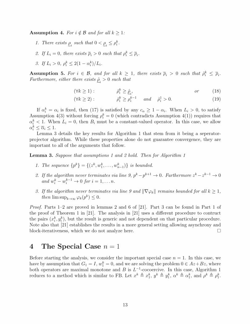
If αki = αi is fixed, then (17) is satisfied by any cα ≥ 1 − αi. When Li > 0, to satisfyAssumption 4(3) without forcing ρki = 0 (which contradicts Assumption 4(1)) requires thatαki < 1. When Li = 0, then Bi must be a constant-valued operator. In this case, we allowαki ≤ αi ≤ 1.

Lemma 3 details the key results for Algorithm 1 that stem from it being a seperator-projector algorithm. While these properties alone do not guarantee convergence, they areimportant to all of the arguments that follow.

Lemma 3. Suppose that assumptions 1 and 2 hold. Then for Algorithm 1

1. The sequence {pk} = {(zk, wk1 , . . . , wkn−1)} is bounded.

2. If the algorithm never terminates via line 9, pk−pk+1 → 0. Furthermore zk−zk−1 → 0and wki − wk−1i → 0 for i = 1, . . . n.

3. If the algorithm never terminates via line 9 and ‖∇ϕk‖ remains bounded for all k ≥ 1,then lim supk→∞ ϕk(p

k) ≤ 0.

Proof. Parts 1–2 are proved in lemmas 2 and 6 of [21]. Part 3 can be found in Part 1 ofthe proof of Theorem 1 in [21]. The analysis in [21] uses a different procedure to contructthe pairs (xki , y

ki ), but the result is generic and not dependent on that particular procedure.

Note also that [21] establishes the results in a more general setting allowing asynchrony andblock-iterativeness, which we do not analyze here.

4 The Special Case n = 1

Before starting the analysis, we consider the important special case n = 1. In this case, wehave by assumption that G1 = I, wk1 = 0, and we are solving the problem 0 ∈ Az+Bz, whereboth operators are maximal monotone and B is L−1-cocoercive. In this case, Algorithm 1reduces to a method which is similar to FB. Let xk , xk1, yk , yk1 , αk , αk1, and ρk , ρk1.

13

Assuming for simplicity that B = {∅}, meaning backtracking is not being used, then theupdates carried out by the algorithm are

xk = JρkA((1− αk)xk−1 + αkzk − ρkBxk−1

)(20)

yk = Bxk +1

ρk((1− αk)xk−1 + αkzk − ρkBxk−1 − xk

)zk+1 = zk − τ kyk, where τ k =

max{〈zk − xk, yk〉, 0}‖yk‖2

.

If αk1 = 0, then for all k ≥ 2, the iterates computed in (20) reduce simply to

xk = JρkA(xk−1 − ρkBxk−1

)which is exactly FB. However, αk1 = 0 is not allowed in our analysis. Thus, FB is a for-bidden boundary case which may be approached by setting αk1 arbitrarily close to 0. Asαk1 approaches 0, the stepsize constraint ρki ≤ 2(1− αki )/L approaches the classical stepsizeconstraint for FB: ρk ≤ 2/L−ε for some arbitrarily small constant ε > 0. A potential benefitof Algorithm 1 over FB in the n = 1 case is that it does allow for backtracking when L isunknown or only a conservative estimate is available.

5 Main Proof

The core of the proof strategy will be to establish (21) below. If this can be done, then weakconvergence to a solution follows from part 3 of Theorem 1 in [21].

Lemma 4. Suppose assumptions 1 and 2 hold and Algorithm 1 produces an infinite sequenceof iterations without terminating via Line 9. If

(∀i = 1, . . . , n) : yki − wki → 0 and Gizk − xki → 0, (21)

then there exists (z,w) ∈ S such that (zk,wk) ⇀ (z,w). Furthermore, xki ⇀ Giz andyki ⇀ wi for all i = 1, . . . , n− 1, xkn ⇀ z, and ykn ⇀ −

∑n−1i=1 G

∗iwi.

Proof. Equivalent to part 3 of the proof of Theorem 1 in [21].

Lemma 4 can be intuitively understood as follows. If we define, for all k ≥ 1,

εk = maxi=1,...,n

{max

{‖yki − wki ‖, ‖Giz

k − xki ‖}}

,

then (21) is equivalent to saying that εk → 0. For all k ≥ 1, we have (xki , yki ) ∈ gra Ti. If

εk = 0, then wki = yki ∈ Tixki = TiGizk and since

∑ni=1G

∗iw

ki = 0, it follows that (zk,wk) ∈ S

and zk solves (3). Thus εk can be thought of as the “residual” of the algorithm whichmeasures how far it is from finding a point in S and a solution to (3). In finite dimension,it is straightforward to show that if εk → 0, (zk,wk) must converge to some element of S.This can be done using Fejer monotonicity [4, Theorem 5.5] combined with the fact thatthe graph of a maximal-monotone operator in a finite-dimensional Hilbert space is closed [4,

14

Proposition 20.38]. However in the general Hilbert space setting the proof is more delicate,since the graph of a maximal-monotone operator is not in-general closed in the weak-to-weak topology [4, Example 20.39]. Nevertheless the overall result was established in thegeneral Hilbert space setting in part 3 of Theorem 1 of [21], which is itself an instance of [1,Proposition 2.4] (see also [4, Proposition 26.5]). An arguably more transparent proof can befound in [16] (this proof is only for the case n = 2, but it can be extended).

In order to establish (21), we start by establishing certain contractive and “ascent” prop-erties for the mapping F , and also show that the backtracking procedure terminates finitely.Then, we prove the boundedness of xki and yki , in turn yielding the boundedness of the gradi-ents ∇ϕk and hence the result that lim supk→∞{ϕk(pk)} ≤ 0 by Lemma 3. Next we establisha “Lyapunov-like” recursion for ϕi,k(z

k, wki ), relating ϕi,k(zk, wki ) to ϕi,k−1(z

k−1, wk−1i ). Even-tually this result will allow us to establish that lim infk ϕk(p

k) ≥ 0 and hence that ϕk(pk)→ 0,

which will in turn allow an argument that yki − wki → 0. The proof that Gizk − xki → 0 will

then follow fairly elementary arguments.The primary innovations of the upcoming proof are the ascent lemma and the way that

it is used in Lemma 17 to establish ϕk(pk) → 0 and yki − wki → 0. This technique is a

significant deviation from previous analyses in the projective splitting family. In previouswork, the strategy was to show that ϕi,k(z

k, wki ) ≥ C max{‖Gizk − xki ‖2, ‖yki − wki ‖2} for a

constant C > 0, which may be combined with lim supϕk(pk) ≤ 0 to imply (21). In contrast,

in the algorithm of this paper we cannot establish such a result and in fact ϕk(pk) may be

negative. Instead, we relate ϕk(pk) to ϕk−1(p

k−1) to show that the separation improves ateach iteration in a way which still leads to overall convergence.

5.1 Some Basic Results

We begin by stating three elementary results on sequences, which may be found in [34], anda basic, well known nonexpansivity property for forward steps with cocoercive operators.

Lemma 5. [34, Lemma 1, Ch. 2] Suppose ak ≥ 0 for all k ≥ 1, b ≥ 0, 0 ≤ τ < 1, andak+1 ≤ τak + b for all k ≥ 1. Then {ak} is a bounded sequence.

Lemma 6. [34, Lemma 3, Ch. 2] Suppose that ak ≥ 0, bk ≥ 0 for all k ≥ 1, bk → 0, andthere is some 0 ≤ τ < 1 such that ak+1 ≤ τak + bk for all k ≥ 1. Then ak → 0.

Lemma 7. Suppose that {rk}, {bk}, and {τk} are sequences in R with bk → 0, and that forall k ≥ 1, we have 0 ≤ τk ≤ τ < 1 and rk+1 ≥ τkrk + bk. Then lim infk→∞{rk} ≥ 0.

Proof. Negating the claimed inequality yields −rk+1 ≤ τk(−rk)− bk. Applying [34, Lemma3, Ch. 2] then yields lim sup{−rk} ≤ 0.

Lemma 8. Suppose B is L−1-cocoercive and 0 ≤ ρ ≤ 2/L. Then for all x, y ∈ dom(B)

‖x− y − ρ(Bx−By)‖ ≤ ‖x− y‖. (22)

Proof. Squaring the left hand side of (22) yields

‖x− y − ρ(Bx−By)‖2 = ‖x− y‖2 − 2ρ〈x− y,Bx−By〉+ ρ2‖Bx−By‖2

≤ ‖x− y‖2 − 2ρ

L‖Bx−By‖2 + ρ2‖Bx−By‖2

≤ ‖x− y‖2.

15

5.2 A Contractive Result

We begin the main proof with a result on the one-forward-step mapping: F from Definition1. The following lemma will ultimately be used to show that the iterates remain bounded.

Lemma 9. Suppose (x+, y+) = Fα,ρ(z, x, w;A,B,G), where Fα,ρ is given in Definition 1.Recall that B is L−1-cocoercive. If L = 0 or ρ ≤ 2(1− α)/L, then

‖x+ − θ‖ ≤ (1− α)‖x− θ‖+ α‖Gz − θ‖+ ρ ‖w − w‖ (23)

for any θ ∈ dom(A) and w ∈ Aθ +Bθ.

Proof. Select any θ ∈ dom(A) and w ∈ Aθ + Bθ. Let a = w − Bθ ∈ Aθ. It followsimmediately from (4) that

θ = JρA(θ + ρa). (24)

Therefore, (16) and (24) yield

‖x+ − θ‖ =∥∥∥JρA((1− α)x+ αGz − ρ(Bx− w)

)− JρA(θ + ρa)

∥∥∥(a)

≤∥∥∥(1− α)x+ αGz − ρ(Bx− w)− θ − ρa

∥∥∥(b)=

∥∥∥∥(1− α)

(x− θ − ρ

1− α

(Bx−Bθ

))+ α(Gz − θ) + ρ

(w − a−Bθ

)∥∥∥∥(c)

≤ (1− α)

∥∥∥∥x− θ − ρ

1− α

(Bx−Bθ

)∥∥∥∥+ α‖Gz − θ‖+ ρ∥∥∥w − (a+Bθ)

∥∥∥ (25)

(d)

≤ (1− α)‖x− θ‖+ α‖Gz − θ‖+ ρ ‖w − w‖ .

To obtain (a), one uses the nonexpansivity of the resolvent [4, Prop. 23.8(ii)]. To obtain (b),one regroups terms and adds and subtracts Bθ. Then (c) follows from the triangle inequality.Finally we consider (d): If L > 0, apply Lemma 8 to the first term on the right-hand side of(25) with the stepsize ρ/(1− α) which by assumption satisfies

ρ

1− α≤ 2

L

by Assumption 4. Alternatively, if L = 0, implying that B is a constant-valued operator,then Bx = Bθ and (d) is just an equality.

We now prove the key “ascent lemma”. It shows that, while the one-forward-step updateis not guaranteed to find a separating hyperplane at each iteration, it does make a certainkind of progress toward separation.

16

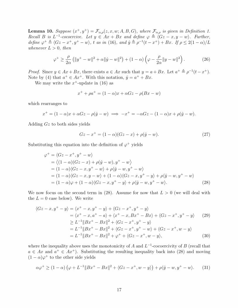
Lemma 10. Suppose (x+, y+) = Fα,ρ(z, x, w;A,B,G), where Fα,ρ is given in Definition 1.Recall B is L−1-cocoercive. Let y ∈ Ax + Bx and define ϕ , 〈Gz − x, y − w〉. Further,define ϕ+ , 〈Gz − x+, y+ − w〉, t as in (16), and y , ρ−1(t− x+) +Bx. If ρ ≤ 2(1− α)/Lwhenever L > 0, then

ϕ+ ≥ ρ

2α

(‖y+ − w‖2 + α‖y − w‖2

)+ (1− α)

(ϕ− ρ

2α‖y − w‖2

). (26)

Proof. Since y ∈ Ax+Bx, there exists a ∈ Ax such that y = a+Bx. Let a+ , ρ−1(t−x+).Note by (4) that a+ ∈ Ax+. With this notation, y = a+ +Bx.

We may write the x+-update in (16) as

x+ + ρa+ = (1− α)x+ αGz − ρ(Bx− w)

which rearranges to

x+ = (1− α)x+ αGz − ρ(y − w) =⇒ −x+ = −αGz − (1− α)x+ ρ(y − w).

Adding Gz to both sides yields

Gz − x+ = (1− α)(Gz − x) + ρ(y − w). (27)

Substituting this equation into the definition of ϕ+ yields

ϕ+ = 〈Gz − x+, y+ − w〉=⟨(1− α)(Gz − x) + ρ(y − w), y+ − w

⟩= (1− α)〈Gz − x, y+ − w〉+ ρ〈y − w, y+ − w〉= (1− α)〈Gz − x, y − w〉+ (1− α)〈Gz − x, y+ − y〉+ ρ〈y − w, y+ − w〉= (1− α)ϕ+ (1− α)〈Gz − x, y+ − y〉+ ρ〈y − w, y+ − w〉. (28)

We now focus on the second term in (28). Assume for now that L > 0 (we will deal withthe L = 0 case below). We write

〈Gz − x, y+ − y〉 = 〈x+ − x, y+ − y〉+ 〈Gz − x+, y+ − y〉= 〈x+ − x, a+ − a〉+ 〈x+ − x,Bx+ −Bx〉+ 〈Gz − x+, y+ − y〉 (29)

≥ L−1‖Bx+ −Bx‖2 + 〈Gz − x+, y+ − y〉= L−1‖Bx+ −Bx‖2 + 〈Gz − x+, y+ − w〉+ 〈Gz − x+, w − y〉= L−1‖Bx+ −Bx‖2 + ϕ+ + 〈Gz − x+, w − y〉, (30)

where the inequality above uses the monotonicity of A and L−1-cocoercivity of B (recall thata ∈ Ax and a+ ∈ Ax+). Substituting the resulting inequality back into (28) and moving(1− α)ϕ+ to the other side yields

αϕ+ ≥ (1− α)(ϕ+ L−1‖Bx+ −Bx‖2 + 〈Gz − x+, w − y〉

)+ ρ〈y − w, y+ − w〉. (31)

17

Using (27) once again, this time to the third term on the right-hand side, we write

〈Gz − x+, w − y〉 =⟨(1− α)(Gz − x) + ρ(y − w), w − y

⟩= (1− α)〈Gz − x,w − y〉+ ρ〈y − w,w − y〉= (α− 1)ϕ− ρ〈y − w, y − w〉. (32)

Substituting this equation back into (31) yields

αϕ+ ≥ (1− α)(αϕ+ L−1‖Bx+ −Bx‖2 − ρ〈y − w, y − w〉

)+ ρ〈y − w, y+ − w〉. (33)

We next use the identity 〈x1, x2〉 = 12‖x1‖2 + 1

2‖x2‖2 − 1

2‖x1 − x2‖2 on both inner products

in the above expression, as follows:

〈y − w, y − w〉 =1

2

(‖y − w‖2 + ‖y − w‖2 − ‖y − y‖2

)=

1

2

(‖y − w‖2 + ‖y − w‖2 − ‖a+ − a‖2

)(34)

and

〈y − w, y+ − w〉 =1

2

(‖y − w‖2 + ‖y+ − w‖2 − ‖y − y+‖2

)=

1

2

(‖y − w‖2 + ‖y+ − w‖2 − ‖Bx+ −Bx‖2

). (35)

Here we have used the identies

y − y = a+ +Bx− (a+Bx) = a+ − ay − y+ = a+ +Bx− (a+ +Bx+) = Bx−Bx+.

Using (34)–(35) in (33) and simplifying yields

αϕ+ ≥ (1− α)(αϕ− ρ

2‖y − w‖2 +

ρ

2‖a+ − a‖2

)+

(1− αL− ρ

2

)‖Bx+ −Bx‖2

+ρ

2

(‖y+ − w‖2 + α‖y − w‖2

).

Now, the coefficient of ‖a+ − a‖2 is nonnegative so this term can be lower-bounded by 0.Furthermore, since ρ ≤ 2(1 − α)/L, the coefficient of ‖Bx+ − Bx‖2 is positive as well, andthis term can also be lower-bounded by 0. Using these bounds and dividing through by α,we obtain (26).

Finally, we deal with the case in which L = 0, which implies that Bx = v for some v ∈ Hfor all x ∈ H. The main difference is that the ‖Bx+ − Bx‖2 terms are no longer presentsince Bx+ = Bx. The analysis is the same up to (28). In this case Bx+ = v so instead of(30) we may deduce from (29) that

〈Gz − x, y+ − y〉 ≥ ϕ+ + 〈Gz − x+, w − y〉.

18

Since Bx+ = Bx = v is constant we also have that

y = a+ +Bx = a+ + v = a+ +Bx+ = y+

Thus, instead of (31) in this case we have the simpler inequality

αϕ+ ≥ (1− α)(ϕ+ 〈Gz − x+, w − y〉

)+ ρ‖y+ − w‖2. (36)

The term 〈Gz−x+, w− y〉 in (36) is dealt with just as in (31), by substitution of (27). Thisstep now leads via (32) to

αϕ+ ≥ α(1− α)ϕ− ρ(1− α)〈y+ − w, y − w〉+ ρ‖y+ − w‖2.

Once again using 〈x1, x2〉 = 12‖x1‖2 + 1

2‖x2‖2 − 1

2‖x1 − x2‖2 on the second term on the

r.h.s. above yields

αϕ+ ≥ α(1− α)ϕ+ ρ‖y+ − w‖2 − ρ(1− α)

2

(‖y+ − w‖2 + ‖y − w‖2 − ‖y+ − y‖2

).

We can lower-bound the ‖y+ − y‖2 term by 0. Dividing through by α and rearranging, weobtain

ϕ+ ≥ ρ(1 + α)

2α‖y+ − w‖2 + (1− α)

(ϕ− ρ

2α‖y − w‖2

).

Since y+ = y in the L = 0 case, this is equivalent to (26).

5.3 Finite Termination of Backtracking

In all the following lemmas in sections 5.3 and 5.4 regarding algorithms 1–3, assumptions1–5 are in effect and will not be explicitly stated in each lemma. We start by proving thatbackTrack terminates in a finite number of iterations, and that the stepsizes it returns arebounded away from 0.

Lemma 11. For i ∈ B, Algorithm 2 terminates in a finite number of iterations for allk ≥ 1. There exists ρ

i> 0 such that ρki ≥ ρ

ifor all k ≥ 1, where ρki is the stepsize returned

by Algorithm 2 on line 4.

Proof. Assume we are at iteration k ≥ 1 in Algorithm 1 and backTrack has been calledthrough line 4 for some i ∈ B. The internal variables within backTrack are defined in termsof the variables passed from Algorithm 1 as follows: z = zk, w = wki , x = xk−1i , y = yk−1i ,

ρ1 = ρki , ϕ = ϕi,k−1(zk, wki ), α = αki , θ = θi, w = wi, A = Ai, B = Bi, and G = Gi. In the

following argument, we mostly refer to the internal name of the variables within backTrack

without explicitly making the above substitutions. With that in mind, let L = Li be thecocoercivity constant of B = Bi.

Observe that backtracking terminates via line 9 if two conditions are met. The firstcondition,

‖xj − θ‖ ≤ (1− α)‖x− θ‖+ α‖Gz − θ‖+ ρj‖w − w‖, (37)

19

is identical to (23) of Lemma 9, with xj and ρj respectively in place of x+ and ρ. The

initialization step of Algorithm 2 provides us with w ∈ Aθ + Bθ for some θ ∈ dom(A).Furthermore, since

(xj, yj) = Fα,ρj(z, x, w;A,B,G),

the findings of Lemma 9 may be applied. In particular, if L > 0 and ρj ≤ 2(1− α)/L, then(37) will be met. Alternatively, if L = 0, (37) will hold for any value of the stepsize ρj > 0.

Next, consider the second termination condition,

ϕ+j ≥

ρj2α

(‖yj − w‖2 + α‖yj − w‖2

)+ (1− α)

(ϕ− ρj

2α‖y − w‖2

). (38)

This relation is identical to (26) of Lemma 10, with (yj, yj, ρj) in place of (y+, y, ρ). However,to apply the lemma we must show that y = yk−1i ∈ Axk−1i + Bxk−1i = Ax+ Bx. We will doso by induction.

For k = 1, y = yk−1i ∈ Axk−1i + Bxk−1i = Ax + Bx holds by the initialization step ofAlgorithm 1. Now assume that it holds at iteration k ≥ 2. We may then apply the findingsof Lemma 10 to conclude the if L > 0 and ρj ≤ 2(1− α)/L, then condition (38) is satisfied.Or, if L = 0, condition (38) is satisfied for any ρj > 0.

Combining the above observations, we conclude that if L > 0 and ρj ≤ 2(1 − α)/L,backtracking will terminate in that iteration via line 9. Or, if L = 0, it will terminate in thefirst iteration. The stepsize decrement condition on line 10 of the backtracking procedureimplies that ρj ≤ 2(1−α)/L will eventually hold for large enough j, and hence that the twobacktracking termination conditions must eventually hold.

Let j∗ ≥ 1 be the iteration at which backtracking terminates when called for operatori at iteration k of Algorithm 1. For the pair (xki , y

ki ) returned by backTrack on line 4 of

Algorithm 1, we may write

(xki , yki ) = (xj∗ , yj∗) = Fα,ρj∗ (z, x, w;A,B,G) = Fαk

i ,ρki(zk, xk−1i , wki ;Ai, Bi, Gi).

Thus, by the definition of F in (16), yki ∈ Aixki + Bix

ki . Therefore, induction establishes

that yki ∈ Aixki + Bixki holds for all k ≥ 1. Inductively, we now also know that backTrack

terminates in a finite number of iterations for all k ≥ 1 and i ∈ B.For all k ≥ 1 and i ∈ B, the returned stepsize ρki = ρj∗ must satisfy

(∀ i : Li > 0) : ρki ≥ min

{ρki ,

2δ(1− αki )Li

}(39)

(∀ i : Li = 0) : ρki = ρki .

If (18) is enforced then we immediately conclude that for i with Li > 0

ρki ≥ min

{ρki ,

2δ(1− αki )Li

}≥ min

{ρi,2δ(1− αi)

Li

}, ρ

i> 0,

20

and similarly for Li = 0, we have ρki ≥ ρi, ρ

i> 0. On the other hand, if (19) is enforced

then we may argue that for all k ≥ 1 and all i ∈ B such that Li > 0, one has

ρki ≥ min

{ρki ,

2δ(1− αi)Li

}≥ min

{ρk−1i ,

2δ(1− αi)Li

}≥ min

{ρ1i ,

2δ(1− αi)Li

}≥ min

{ρ1i ,

2δ(1− αi)Li

}, ρ

i> 0,

where the second inequality uses (19), the third inequality recurses, and the final inequalityis just (39) for k = 1. If Li = 0, the argument is simply

ρki = ρki ≥ ρk−1i = ρk−1i ≥ . . . ≥ ρ1i , ρi> 0.

5.4 Boundedness Results and their Direct Consequences

Lemma 12. For i = 1, . . . , n

‖xki − θi‖ ≤ (1− αki )‖xk−1i − θi‖+ αki ‖Gizk − θi‖+ ρki

∥∥wki − wi∥∥ (40)

for some θi ∈ dom(Ai) and wi ∈ Aθi +Bθi.

Proof. For i ∈ B, Lemma 11 establishes that backTrack terminates for finite j ≥ 1 for allk ≥ 1. For fixed k ≥ 1 and i ∈ B, let j∗ ≥ 1 be the iteration of backTrack that terminates.At termination, the following condition is satisfied via line 7:

‖xj∗ − θ‖ ≤ (1− α)‖x− θ‖+ α‖Gz − θ‖+ ρj∗‖w − w‖.

Into this inequality, now substitute in the following variables from Algorithm 1, as passed toand from backTrack: xki = xj∗ , θi = θ, αki = α, xk−1i = x, Gi = G, zk = z, ρki = ρj∗ , w

ki = w,

and wi = w. The result is (40).For i /∈ B, we note that line 6 of Algorithm 1 reads as

(xki , yki ) = Fαk

i ,ρki(zk, xk−1i , wki ;Ai, Bi, Gi)

and Assumption 4(3) holds, so we may apply Lemma 9 to yield (40).

Lemma 13. For all i = 1, . . . , n, the sequences {xki } and {yki } are bounded.

Proof. Fix any i ∈ {1, . . . , n}. From (40) and the bounds on {αki } and {ρki }, we have

(∀ k ≥ 1) ‖xki − θi‖ ≤ (1− αi)‖xk−1i − θi‖+ αi‖Gizk − θi‖+ ρi

∥∥wki − wi∥∥ .Since {zk}, and {wki } are bounded by Lemma 3 and ‖Gi‖ is bounded by Assumption 1,boundedness of {xki } now follows by applying Lemma 5 with τ = 1− αi < 1.

Next, boundedness of Bixki follows from the continuity of Bi. Since Lemma 11 established

that backTrack terminates in a finite number of iterations we have for any k ≥ 2 that

(xki , yki ) = Fαk

i ,ρki(zk, xk−1i , wki ;Ai, Bi, Gi).

Expanding the y+-update in the definition of F in (16), we may write

yki = (ρki )−1 ((1− αki )xk−1i + αkiGiz

k − ρki (Bixk−1i − wki )− xki

)+Bxki .

Since 0 ≤ αki ≤ 1, Gi, zk, and wki are bounded, ρki ≤ ρi, and ρki ≥ ρ

i(using Lemma 11 for

i ∈ B), we conclude that yki remains bounded.

21

With {xki } and {yki } bounded for all i = 1, . . . , n, the boundedness of ∇ϕk follows imme-diately:

Lemma 14. The sequence {∇ϕk} is bounded. If Algorithm 1 never terminates via line 9,lim supk→∞ ϕk(p

k) ≤ 0.

Proof. By Lemma 2, ∇zϕk =∑n

i=1G∗i yki , which is bounded since each Gi is bounded by

assumption and each {yki } is bounded by Lemma 13. Furthermore, ∇wiϕk = xki − Gix

kn is

bounded using the same two lemmas. That lim supk→∞ ϕk(pk) ≤ 0 then immediately follows

from Lemma 3(3).

Using the boundedness of {xki } and {yki }, we can next derive the following simple boundrelating ϕi,k−1(z

k, wki ) to ϕi,k−1(zk−1, wk−1i ):

Lemma 15. There exists M1,M2 ≥ 0 such that for all k ≥ 2 and i = 1, . . . , n,

ϕi,k−1(zk, wki ) ≥ ϕi,k−1(z

k−1, wk−1i )−M1‖wki − wk−1i ‖ −M2‖Gi‖‖zk − zk−1‖.

Proof. For each i ∈ {1, . . . , n}, let M1,i,M2,i ≥ 0 be respective bounds on{‖Giz

k−1−xk−1i ‖}

and{‖yk−1i −wki ‖

}, which must exist by Lemma 3, the boundedness of {xki } and {yki }, and

the boundedness of Gi. Let M1 = maxi=1,...,m{M1,i} and M2 = maxi=1,...,m{M2,i}. Then, forany k ≥ 2 and i ∈ {1, . . . , n}, we may write

ϕi,k−1(zk, wki ) = 〈Giz

k − xk−1i , yk−1i − wki 〉= 〈Giz

k−1 − xk−1i , yk−1i − wki 〉+ 〈Gizk −Giz

k−1, yk−1i − wki 〉= 〈Giz

k−1 − xk−1i , yk−1i − wk−1i 〉+ 〈Gizk−1 − xk−1i , wk−1i − wki 〉

+ 〈Gizk −Giz

k−1, yk−1i − wki 〉≥ ϕi,k−1(z

k−1, wk−1i )−M1‖wki − wk−1i ‖ −M2‖Gi‖‖zk − zk−1‖,

where the last step uses the Cauchy-Schwarz inequality and the definitions of M1 and M2.

5.5 A Lyapunov-Like Recursion for the Hyperplane

We now establish a Lyapunov-like recursion for the hyperplane. For this purpose, we needone more definition and assumption.

Definition 2. For all k ≥ 1, since Lemma 11 establishes that Algorithm 2 terminates in afinite number of iterations, we may write for i = 1, . . . , n:

(xki , yki ) = Fαk

i ,ρki(zk, xk−1i , wki ;Ai, Bi, Gi).

Using (4) and the x+-update in (16), there exists aki ∈ Aixki such that

xki + ρki aki = (1− αki )xk−1i + αkiGiz

k − ρki (Bixk−1i − wki ).

Define yki , aki +Bixk−1i .

22

Assumption 6. For all k ≥ 1, and i /∈ B, αki and ρki are chosen to satisfy

ρk+1i

αk+1i

‖yki − wki ‖2 ≤ρkiαki

(‖yki − wki ‖2 + αki ‖yki − wki ‖2

). (41)

On the other hand, for i ∈ B, the initial trial stepsizes ρki and αki are chosen to satisfy:

ρk+1i

αk+1i

‖yki − wki ‖2 ≤ρkiαki

(‖yki − wki ‖2 + αki ‖yki − wki ‖2

)(42)

where ρki is returned on line 4.

If αki = αi is fixed, (42) would then be guaranteed by choosing ρk+1i ≤ ρki . However

for fixed αki , (42) allows the trial stepsize to increase by some factor times the previouslydiscovered stepsize. In practice we have observed that ‖yki − wki ‖ and ‖yki − wki ‖ tend to beapproximately equal, so (42) allows for an increase in the trial stepsize by up to a factor ofapproximately 1 + αi.

In addition to assumptions 1–5, Assumption 6 is now in effect and will not be explicitlystated in the upcoming lemmas of sections 5.5–5.6.

Lemma 16. For all k ≥ 2 and i = 1, . . . , n,

ϕi,k(zk, wki )−

ρki2αki

(‖yki − wki ‖2 + αki ‖yki − wki ‖2

)≥ (1− αki )

(ϕi,k−1(z

k, wki )−ρki

2αki‖yk−1i − wki ‖2

)(43)

and

ϕi,k(zk, wki )−

ρk+1i

2αk+1i

‖yki − wki ‖2 ≥ (1− αki )(ϕi,k−1(z

k, wki )−ρki

2αki‖yk−1i − wki ‖2

). (44)

Proof. Take any i ∈ B. Lemma 11 guarantees the finite termination of backTrack. Nowconsider the backtracking termination condition

ϕ+j ≥

ρj2α

(‖yj − w‖2 + α‖yj − w‖2

)+ (1− α)

(ϕ− ρj

2α‖y − w‖2

).

Fix some k ≥ 2, and let j∗ ≥ 1 be the iteration at which backTrack terminates. In theabove inequality, make the following substitutions for the internal variables of backTrack bythose passed in/out of the function: ϕi,k(z

k, xki ) = ϕ+j∗ , ρ

ki = ρj∗ , α

ki = α, yki = yj, w

ki = w,

ϕi,k−1(zk, wki ) = ϕ. Furthermore, yki = yj∗ where yki is defined in Definition 2. Together,

these substitutions yield (43). We can then apply (42), along with ρk+1i ≤ ρk+1

i , to produce(44).

Now take any i ∈ {1, . . . , n}\B. From line 6 of Algorithm 1, Assumption 4(3), andLemma 10, we directly deduce (43). Combining this relation with (41) we obtain (44).

23

5.6 Finishing the Proof

We now work toward establishing the conditions of Lemma 4, which we then apply. Unlessotherwise specified, we henceforth assume that Algorithm 1 runs indefinitely and does notterminate at line 9.

Lemma 17. For all i = 1, . . . , n, we have yki − wki → 0 and ϕk(pk)→ 0.

Proof. Fix any i ∈ {1, . . . , n}. First, note that for all k ≥ 2,

‖yk−1i − wki ‖2 = ‖yk−1i − wk−1i ‖2 + 2〈yk−1i − wk−1i , wk−1i − wki 〉+ ‖wk−1i − wki ‖2

≤ ‖yk−1i − wk−1i ‖2 +M3‖wki − wk−1i ‖+ ‖wki − wk−1i ‖2

= ‖yk−1i − wk−1i ‖2 + dki , (45)

where dki , M3‖wki − wk−1i ‖ + ‖wki − wk−1i ‖2 and M3 ≥ 0 is a bound on 2‖yk−1i − wk−1i ‖,which must exist because both {yki } and {wki } are bounded by lemmas 3 and 13. Note thatdki → 0 as a consequence of Lemma 3.

Second, recall Lemma 15, which states that there exists M1,M2 ≥ 0 such that for allk ≥ 2,

ϕi,k−1(zk, wki ) ≥ ϕi,k−1(z

k−1, wk−1i )−M1‖wk−1i − wki ‖ −M2‖Gi‖‖zk − zk−1‖. (46)

Now let, for all k ≥ 1,

rki , ϕi,k(zk, wki )−

ρk+1i

2αk+1i

‖yki − wki ‖2, (47)

so that

n∑i=1

rki = ϕk(pk)−

n∑i=1

ρk+1i

2αk+1i

‖yki − wki ‖2. (48)

Using (45) and (46) in (44) yields

(∀k ≥ 2) : rki ≥ (1− αki )rk−1i + eki (49)

where

eki , −(1− αki )(ρki

2αkidki +M1‖wk−1i − wki ‖+M2‖Gi‖‖zk − zk−1‖

). (50)

Note that ρki is bounded, 0 < αki ≤ 1, ‖Gi‖ is finite, ‖zk−zk−1‖ → 0 and ‖wki −wk−1i ‖ → 0by Lemma 3, and dki → 0. Thus eki → 0.

Since 0 < αi ≤ αki ≤ 1, we may apply Lemma 7 to (49) with τk = 1−αki and τ = 1−αi < 1which yields lim infk→∞{rki } ≥ 0. Therefore

lim infk→∞

n∑i=1

rki ≥n∑i=1

lim infk→∞

rki ≥ 0. (51)

24

On the other hand, lim supk→∞ ϕk(pk) ≤ 0 by Lemma 14. Therefore, using (48) and (51),

0 ≤ lim infk→∞

n∑i=1

rki = lim infk→∞

{ϕk(p

k)−n∑i=1

ρk+1i

2αk+1i

‖yki − wki ‖2}

≤ lim infk→∞

ϕk(pk) ≤ lim sup

k→∞ϕk(p

k) ≤ 0.

Therefore limk→∞{ϕk(p

k)}

= 0. Consider any i ∈ {1, . . . , n}. Combining limk→∞{ϕk(p

k)}

=0 with lim infk→∞

∑ni=1 r

ki ≥ 0, we have

lim supk→∞

{(ρk+1i /αk+1

i )‖yki − wki ‖2}≤ 0 ⇒ (ρk+1

i /αk+1i )‖yki − wki ‖2 → 0.

Since ρki ≥ ρi> 0 (using Lemma 11 for i ∈ B) and αki ≤ αi, we conclude that yki −wki → 0.

We have already proved the first requirement of Lemma 4, that yki − wki → 0 for alli ∈ {1, . . . , n}. We now work to establish the second requirement, that Giz

k − xki → 0. Inthe upcoming lemmas we continue to use the quantity yki which is given in Definition 2.

Lemma 18. Recall {yki }k∈N from Definition 2. For all i = 1, . . . , n, yki − wki → 0.

Proof. Fix any k ≥ 1. For all i = 1, . . . , n, repeating (43) from Lemma 16, we have

ϕi,k(zk, wki ) ≥ (1− αki )

(ϕi,k−1(z

k, wki )−ρki

2αki‖yk−1i − wki ‖2

)+

ρki2αki

(‖yki − wki ‖2 + αki ‖yki − wki ‖2

)≥ (1− αki )rk−1i +

ρki2‖yki − wki ‖2 + eki

where we have used rki defined (47) along with (45)–(46) and eki is defined in (50). This isthe same argument used in Lemma 17, but now we apply (45)–(46) to (43), rather than (44),so that we can upper bound the ‖yki − wki ‖2 term. Summing over i = 1, . . . , n, yields

ϕk(pk) =

n∑i=1

ϕi,k(zk, wki ) ≥

n∑i=1

(1− αki )rk−1i +n∑i=1

ρki2‖yki − wki ‖2 +

n∑i=1

eki .

Since ϕk(pk) → 0, eki → 0, lim infk→∞{rki } ≥ 0, ρki ≥ ρ

i> 0 for all k, and αki ≤ 1 for all k,

the above inequality implies that yki − wki → 0.

Lemma 19. For i = 1 . . . , n, xki − xk−1i → 0.

Proof. Fix i ∈ {1, . . . , n}. Using the definition of aki in Definition 2, we have for k ≥ 1 that

xki + ρki aki = (1− αki )xk−1i + αkiGiz

k − ρki (Bixk−1i − wki ).

Using the definition of yki , also in Definition 2, this implies that

(∀k ≥ 1) : xki = (1− αki )xk−1i + αkiGizk − ρki (yki − wki ), (52)

(∀k ≥ 2) : xk−1i = (1− αk−1i )xk−2i + αk−1i Gizk−1 − ρk−1i (yk−1i − wk−1i ). (53)

25

Subtracting the second of these equations from the first yields, for all k ≥ 2,

xki − xk−1i = (1− αki )xk−1i + αkiGizk − ρki (yki − wki )− (1− αk−1i )xk−2i

− αk−1i Gizk−1 + ρk−1i (yk−1i − wk−1i )

= (1− αki )(xk−1i − xk−2i ) + (αk−1i − αki )xk−2i + αki (Gizk −Giz

k−1)

− (αk−1i − αki )Gizk−1 + ρk−1i (yk−1i − wk−1i )− ρki (yki − wki ).

= (1− αki )(xk−1i − xk−2i ) + αkiGi(zk − zk−1)

+ (αk−1i − αki )(xk−2i −Gizk−1) + ρk−1i (yk−1i − wk−1i )− ρki (yki − wki ). (54)

Next, (53) can be rearranged into

xk−2i −Gizk−1 = − 1

αk−1i

(xk−1i − xk−2i + ρk−1i (yk−1i − wk−1i )

).

Substituting this equation into (54) yields

xki − xk−1i =

(1− αki −

αk−1i − αkiαk−1i

)(xk−1i − xk−2i )− ρki (yki − wki )

+ ρk−1i

(1− αk−1i − αki

αk−1i

)(yk−1i − wk−1i ) + αkiGi(z

k − zk−1)

= αki

(1

αk−1i

− 1

)(xk−1i − xk−2i )− ρki (yki − wki ) +

ρk−1i αkiαk−1i

(yk−1i − wk−1i )

+ αkiGi(zk − zk−1).

Taking norms and using the triangle inequality yields, for all k ≥ 2, that

‖xki − xk−1i ‖ ≤ αki

(1

αk−1i

− 1

)‖xk−1i − xk−2i ‖+ eki ≤ cα‖xk−1i − xk−2i ‖+ eki , (55)

where

eki =ρk−1i αkiαk−1i

‖yk−1i − wk−1i ‖+ ρki ‖yki − wki ‖+ ‖Gi‖ ‖zki − zk−1i ‖

and cα is defined in Assumption 4. When taking norms we used that 0 < αk−1i ≤ 1 andtherefore that 1/αk−1i −1 ≥ 0. In the second inequality in (55) we used condition (17). Sinceρki is bounded from above and αki is bounded away from 0 and above, eki → 0 using Lemma18, the finiteness of ‖Gi‖, and Lemma 3. Furthermore, cα < 1 by Assumption 4, so we mayapply Lemma 6 to (55) to conclude that xki − xk−1i → 0.

Lemma 20. For i = 1, . . . , n, Gizk − xki → 0.

Proof. Recalling (52), we first write

xki = (1− αki )xk−1i + αkiGizk − ρki (yki − wki )

⇔ αki(Giz

k − xki)

= (1− αki )(xki − xk−1i ) + ρki (yki − wki ). (56)

26

Since {αki } is bounded, Lemma 19 implies that the first term on the right-hand side of (56)converges to zero. Since {ρki } is bounded, Lemma 18 implies that the second term on theright-hand side also converges to zero. Therefore αki ‖Giz

k − xki ‖ → 0. The claimed resultthen follows because {αki } is bounded away from 0.

Finally, we can state our convergence result for Algorithm 1:

Theorem 1. Suppose that assumptions 1-6 hold. If Algorithm 1 terminates by reachingline 9, then its final iterate is a member of the extended solution set S. Otherwise, thesequence {(zk,wk)} generated by Algorithm 1 converges weakly to some point (z,w) in theextended solution set S of (2) defined in (5). Furthermore, xki ⇀ Giz and yki ⇀ wi for alli = 1, . . . , n− 1, xkn ⇀ z, and ykn ⇀ −

∑n−1i=1 G

∗iwi.

Proof. For the finite termination result we refer to Lemma 5 of [21]. Otherwise, lemmas 17and 20 imply that the hypotheses of Lemma 4, hold, and the result follows.

6 Numerical Experiments

All our numerical experiments were implemented in Python (using numpy) on an Intel Xeonworkstation running Linux. We restricted our attention to algorithms with comparablefeatures and benefits to our proposed method. Thus we only considered methods that:

1. Are first-order and “fully split” the problem (that is, separate the linear operators Gi

from the resolvent calculations, and use gradient-type steps for smooth functions),

2. Do not (either approximately or exactly) solve a linear system of equations at eachiteration or before the first iteration,

3. Avoid having to apply “smoothing” to nonsmooth operators,

4. Incorporate a backtracking linesearch in a manner that avoids the need for bounds onLipschitz or cocoercivity constants, and

5. Do not use iterative approximation of resolvents.

The last property we include for reasons of simplicity, while the rest contribute to makingalgorithms scalable and easy to apply. For a given application, there may of course beeffective algorithms which could have been considered but do not satisfy all of the aboverequirements. However, because of the general desirability of properties 1-4 and the relativesimplicity of algorithms with property 5, we only considered methods having all of them.

We compared this paper’s backtracking one-forward-step projective splitting algorithmgiven in Algorithm 1 (which we call ps1fbt) with the following methods:

• The two-forward-step projective splitting algorithm with backtracking we developedin [21] (ps2fbt). This method requires only Lipschitz continuity of single-valued op-erators, as opposed to cocoercivity.

27

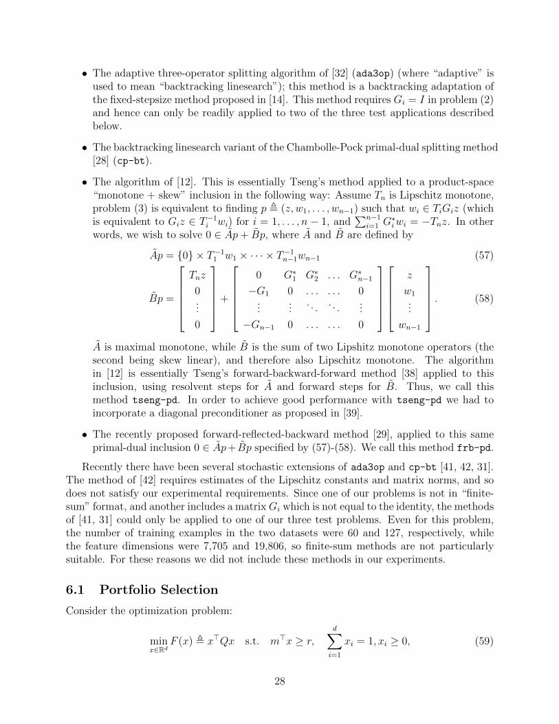
• The adaptive three-operator splitting algorithm of [32] (ada3op) (where “adaptive” isused to mean “backtracking linesearch”); this method is a backtracking adaptation ofthe fixed-stepsize method proposed in [14]. This method requires Gi = I in problem (2)and hence can only be readily applied to two of the three test applications describedbelow.

• The backtracking linesearch variant of the Chambolle-Pock primal-dual splitting method[28] (cp-bt).

• The algorithm of [12]. This is essentially Tseng’s method applied to a product-space“monotone + skew” inclusion in the following way: Assume Tn is Lipschitz monotone,problem (3) is equivalent to finding p , (z, w1, . . . , wn−1) such that wi ∈ TiGiz (whichis equivalent to Giz ∈ T−1i wi) for i = 1, . . . , n − 1, and

∑n−1i=1 G

∗iwi = −Tnz. In other

words, we wish to solve 0 ∈ Ap+ Bp, where A and B are defined by

Ap = {0} × T−11 w1 × · · · × T−1n−1wn−1 (57)

Bp =

Tnz

0...

0

+

0 G∗1 G∗2 . . . G∗n−1−G1 0 . . . . . . 0

......

. . . . . ....

−Gn−1 0 . . . . . . 0

z

w1...

wn−1

. (58)

A is maximal monotone, while B is the sum of two Lipshitz monotone operators (thesecond being skew linear), and therefore also Lipschitz monotone. The algorithmin [12] is essentially Tseng’s forward-backward-forward method [38] applied to thisinclusion, using resolvent steps for A and forward steps for B. Thus, we call thismethod tseng-pd. In order to achieve good performance with tseng-pd we had toincorporate a diagonal preconditioner as proposed in [39].

• The recently proposed forward-reflected-backward method [29], applied to this sameprimal-dual inclusion 0 ∈ Ap+ Bp specified by (57)-(58). We call this method frb-pd.

Recently there have been several stochastic extensions of ada3op and cp-bt [41, 42, 31].The method of [42] requires estimates of the Lipschitz constants and matrix norms, and sodoes not satisfy our experimental requirements. Since one of our problems is not in “finite-sum” format, and another includes a matrixGi which is not equal to the identity, the methodsof [41, 31] could only be applied to one of our three test problems. Even for this problem,the number of training examples in the two datasets were 60 and 127, respectively, whilethe feature dimensions were 7,705 and 19,806, so finite-sum methods are not particularlysuitable. For these reasons we did not include these methods in our experiments.

6.1 Portfolio Selection

Consider the optimization problem:

minx∈Rd

F (x) , x>Qx s.t. m>x ≥ r,d∑i=1

xi = 1, xi ≥ 0, (59)

28

where Q � 0, r > 0, and m ∈ Rd+. This model arises in Markowitz portfolio theory. We

chose this particular problem because it features two constraint sets (a general halfspace anda simplex) onto which it is easy to project individually, but whose intersection poses a moredifficult projection problem. This property makes it difficult to apply first-order methodssuch as ISTA/FISTA [5] as they can only perform one projection per iteration and thus can-not fully split the problem. On the other hand, projective splitting can handle an arbitrarynumber of constraint sets so long as one can compute projections onto each of them. Weconsider a fairly large instance of this problem so that standard interior point methods (forexample, those in the CVXPY [15] package) are disadvantaged by their high per-iterationcomplexity and thus not generally competitive with first-order methods. Furthermore, back-tracking variants of first-order methods are preferable for large problems as they avoid theneed to estimate the largest eigenvalue of Q.

To convert (59) to a monotone inclusion, we set A1 = NC1 where NC1 is the normalcone of the simplex C1 = {x ∈ Rd :

∑di=1 xi = 0, xi ≥ 0}. We set B1 = 2Qx, which is the

gradient of the objective function and is cocoercive (and Lipschitz-continuous). Finally, weset A2 = NC2 , where C2 = {x : m>x ≥ r}, and let B2 be the zero operator. Note that theresolvents of NC1 and NC2 (that is, the projections onto C1 and C2) are easily computed inO(d) operations [30]. With this notation, one may write (59) as the the problem of findingz ∈ Rd such that

0 ∈ A1z +B1z + A2z,

which is an instance of (2) with n = 2 and G1 = G2 = I.To terminate each method in our comparisons, we used the following common criterion

incorporating both the objective function and the constraints of (59):

c(x) , max

{F (x)− F ∗

F ∗, 0

}−min{m>x− r, 0}+

∣∣∣∣∣d∑i=1

xi − 1

∣∣∣∣∣−max{0,minixi}, (60)

where F ∗ is the optimal value of the problem. Note that c(x) = 0 if and only if x solves(59). To estimate F ∗, we used the best feasible value returned by any method after 1000iterations.

We generated random instances of (59) as follows: we set d = 10, 000 to obtain a relativelylarge instance of the problem. We then generated a d× d matrix Q0 with each entry drawnfrom N (0, 1). The matrix Q is then formed as (1/d) · Q0Q

>0 , which is guaranteed to be

positive semidefinite. We then generate the vector m ∈ Rd of length d to have entriesuniformly distributed between 0 and 100. The constant r is set to δr

∑di=1mi/d for various

values of δr > 0. We solved the problem for δr ∈ {0.5, 0.8, 1, 1.5}.All methods were initialized at the same point [1 1 . . . 1]>/d. For all the backtracking

linesearch procedures except cp-bt , the initial stepsize estimate is the previously discoveredstepsize; at the first iteration, the initial stepsize is 1. For cp-bt we allowed the stepsizeto increase in accordance with [28, Algorithm 4], as performance was poor otherwise. Thebacktracking stepsize decrement factor (δ in Algorithm 2) was 0.7 for all algorithms.

For ps1fbt and ps2fbt, ρk1 was discovered via backtracking. We also set the otherstepsize ρk2 equal to ρk1 at each iteration. While this is not necessary, this heuristic performed

29

δr

0.5 0.8 1 1.5

ps1fbt (γ) 0.01 0.01 0.5 5

ps2fbt (γ) 0.1 0.1 10 10

cp-bt (β−1) 1 1 2 2

tseng-pd (γpd) 1 1 1 10

frb-pd (γpd) 1 1 10 10

Table 1: Tuning parameters for the portfolio problem (ada3op does not have a tuning pa-rameter.)

well and eliminated ρk2 as a separately tunable parameter. For the averaging parameters inps1fbt, we used αk1 fixed to 0.1 and αk2 fixed to 1 (which is allowed because L2 = 0). Forps1fbt we set θ1 = x01 and w1 = 2Qx01.

For tseng-pd and frb-pd, we used the following preconditioner:

U = diag(Id×d, γpdId×d, γpdId×d) (61)

where U is used as in [39, Eq. (3.2)] for tseng-pd (M−1 on [29, p. 7] for frb-pd). In thiscase, the “monotone + skew” primal-dual inclusion described in (57)-(58) features two d-dimensional dual variables in addition to the d-dimensional primal variable. The parameterγpd changes the relative size of the steps taken in the primal and dual spaces, and plays asimilar role to γ in our algorithm (see Algorithm 3). The parameter β in [28, Algorithm 4]plays a similar role for cp-bt. For all of these methods, we have found that performance ishighly sensitive to this parameter: the primal and dual stepsizes need to be balanced. Theonly method not requiring such tuning is ada3op, which is a purely primal method. Withthis setup, all the methods have one tuning parameter except ada3op , which has none. Foreach method, we manually tuned the parameter for each δr; Table 1 shows the final choices.

We calculated the criterion c(x) in (60) for xk1 computed by ps1fbt and ps2fbt, xtcomputed on Line 3 of [32, Algorithm 1] for ada3op, yk computed in [28, Algorithm 4] forcp-bt, and the primal iterate for tseng-pd and frb-pd. Table 2 displays the average numberiterations and running time, over 10 random trials, until c(x) falls (and stays) below 10−5

for each method. Examining the table,

• For all four problems, ps1fbt outperforms ps2fbt. This behavior is not suprising, asps1fbt only requires one forward step per iteration, rather than two. Since the matrixQ is large and dense, reducing the number of forward steps should have a sizableimpact.

• For δr < 1, ps1fbt is the best-performing method. However, for δr ≥ 1, ada3op is thequickest.

30

δr

0.5 0.8 1 1.5

ps1fbt 3.6 (102) 4.7 (102) 16.3 (583) 8.5 (255.2)

ps2fbt 5.0 (151.1) 7.9 (155) 24.3 (523.4) 9.2 (222.9)

ada3op 5.3 (180.8) 9.2 (180.8) 6.8 (174.3) 3.4 (89.2)

cp-bt 6.2 (136) 8.3 (134.3) 11.8 (218.4) 5.6 (113.6)

tseng-pd 15.9 (387.1) 21 (387.8) 25.7 (525.3) 11.1 (245.4)

frb-pd 10.5 (559.9) 16.4 (560.4) 22.8 (1074.8) 6.3 (350.8)

Table 2: For the portfolio problem, average running times in seconds and iterations (inparentheses) for each method until c(x) < 10−5 for all subsequent iterations across 10 trials.The best time in each column is in bold.

6.2 Sparse Group Logistic Regression

Consider the following problem:

minx0∈Rx∈Rd

{n∑i=1

log(

1 + exp(− yi(x0 + a>i x)

))+ λ1‖x‖1 + λ2

∑g∈G

‖xg‖2

}, (62)

where ai ∈ Rd and yi ∈ {±1} for i = 1, . . . , n are given data, λ1, λ2 ≥ 0 are regularizationparameters, and G is a set of subsets of {1, . . . , d} such that no element is in more thanone group g ∈ G. This is the non-overlapping group-sparse logistic regression problem,which has applications in bioinformatics, image processing, and statistics [35]. It is wellunderstood that the `1 penalty encourages sparsity in the solution vector. On the otherhand the group-sparse penalty encourages group sparsity, meaning that as λ2 increases moregroups in the solution will be set entirely to 0. The group-sparse penalty can be used whenthe features/predictors can be put into correlated groups in a meaningful way. As with theportfolio experiment, this problem features two nonsmooth regularizers and so methods likeFISTA cannot easily be applied.

Problem (62) may be treated as a special case of (1) with n = 2, G1 = G2 = I, and

h1(x0, x) =n∑i=1

log(

1 + exp(− yi(x0 + a>i x)

))h2(x0, x) = 0

f1(x0, x) = λ1‖x‖1 f2(x0, x) = λ2∑g∈G

‖xg‖2.

Since the logistic regression loss has a Lipschitz-continuous gradient and the `1-norm andnon-overlapping group-lasso penalties both have computationally simple proximal operators,all our candidate methods may be applied.

We applied 62 to two bioinformatics classification problems with real data. Follow-ing [35], we use the breast cancer dataset of [25] and the inflammatory bowel disease (IBD)

31

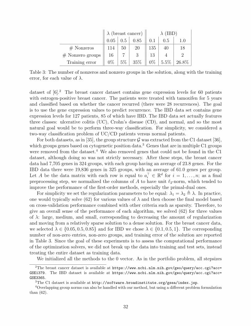
λ (breast cancer) λ (IBD)

0.05 0.5 0.85 0.1 0.5 1.0

# Nonzeros 114 50 20 135 40 18

# Nonzero groups 16 7 3 13 4 2

Training error 0% 5% 35% 0% 5.5% 26.8%

Table 3: The number of nonzeros and nonzero groups in the solution, along with the trainingerror, for each value of λ.

dataset of [6].2 The breast cancer dataset contains gene expression levels for 60 patientswith estrogen-positive breast cancer. The patients were treated with tamoxifen for 5 yearsand classified based on whether the cancer recurred (there were 28 recurrences). The goalis to use the gene expression values to predict recurrence. The IBD data set contains geneexpression levels for 127 patients, 85 of which have IBD. The IBD data set actually featuresthree classes: ulcerative colitis (UC), Crohn’s disease (CD), and normal, and so the mostnatural goal would be to perform three-way classification. For simplicity, we considered atwo-way classification problem of UC/CD patients versus normal patients.

For both datasets, as in [35], the group structure G was extracted from the C1 dataset [36],which groups genes based on cytogenetic position data.3 Genes that are in multiple C1 groupswere removed from the dataset.4 We also removed genes that could not be found in the C1dataset, although doing so was not strictly necessary. After these steps, the breast cancerdata had 7,705 genes in 324 groups, with each group having an average of 23.8 genes. For theIBD data there were 19,836 genes in 325 groups, with an average of 61.0 genes per group.Let A be the data matrix with each row is equal to a>i ∈ Rd for i = 1, . . . , n; as a finalpreprocessing step, we normalized the columns of A to have unit `2-norm, which tended toimprove the performance of the first-order methods, especially the primal-dual ones.

For simplicity we set the regularization parameters to be equal: λ1 = λ2 , λ. In practice,one would typically solve (62) for various values of λ and then choose the final model basedon cross-validation performance combined with other criteria such as sparsity. Therefore, togive an overall sense of the performance of each algorithm, we solved (62) for three valuesof λ: large, medium, and small, corresponding to decreasing the amount of regularizationand moving from a relatively sparse solution to a dense solution. For the breast cancer data,we selected λ ∈ {0.05, 0.5, 0.85} and for IBD we chose λ ∈ {0.1, 0.5, 1}. The correspondingnumber of non-zero entries, non-zero groups, and training error of the solution are reportedin Table 3. Since the goal of these experiments is to assess the computational performanceof the optimization solvers, we did not break up the data into training and test sets, insteadtreating the entire dataset as training data.

We initialized all the methods to the 0 vector. As in the portfolio problem, all stepsizes

2The breast cancer dataset is available at https://www.ncbi.nlm.nih.gov/geo/query/acc.cgi?acc=

GSE1379. The IBD dataset is available at https://www.ncbi.nlm.nih.gov/geo/query/acc.cgi?acc=

GSE3365.3The C1 dataset is available at http://software.broadinstitute.org/gsea/index.jsp.4Overlapping group norms can also be handled with our method, but using a different problem formulation

than (62).

32

λ (breast cancer) λ (IBD)

0.05 0.5 0.85 0.1 0.5 1.0

ps1fbt (γ) 0.05 102 102 0.1 1 1

ps2fbt (γ) 1 102 105 1 1 1

cp-bt (β−1) 10 103 104 104 103 105

tseng-pd (γpd) 103 105 105 104 106 106

frb-pd (γpd) 103 105 105 104 106 106

Table 4: Tuning parameters for sparse group LR (ada3op does not have a tuning parameter).

were initially set to 1. Since the logistic regression function does not have uniform curvature,we allowed the initial trial stepsize in the backtracking linesearch to increase by a factor of 1.1multiplied by the previously discovered stepsize. The methods ps1fbt, cp-bt, and ada3op

have an upper bound on the trial stepsize at each iteration, so the trial stepsize was takento be the minimum of 1.1 multiplied by the previous stepsize and this upper bound.

Otherwise, the setup was the same as the portfolio experiment. tseng-pd and frb-pd

use the same preconditioner as given in (61). For ps1fbt and ps2fbt we set ρk2 to be equalto the discovered backtracked stepsize ρk1 at each iteration. For ps1fbt we again set θ1 = x01,w1 = ∇h1(x01), and αk1 fixed to 0.1. As such, all methods (except ada3op) have one tuningparameter which was hand-picked for each method; the chosen values are given in Table 4.

Figure 1: Results for (62) applied to bioinformatics classification problems. The top rowshows breast cancer data with left: λ = 0.05; middle: λ = 0.5; right: λ = 0.85. The bottomrow shows IBD data with left: λ = 0.1; middle: λ = 0.5; right: λ = 1.0. The y-axis is relativeobjective error:

(F (x0, x)− F ∗

)/F ∗ and the x-axis is elapsed running time in seconds.

Figure 1 shows the results of the experiments, plotting (F (x0, x)− F ∗)/F ∗ against time

33

for each algorithm, where F is the objective function in (62) and F ∗ is the estimated optimalvalue. To approximate F ∗, we ran each algorithm for 4,000 iterations and took the lowestvalue obtained. Overall, ps1fbt and ada3op were much faster than the other methods. Forthe highly regularized cases (the right column of the figure), ps1fbt was faster than all othermethods. For middle and low regularization, ps1fbt and ada3op are comparable, and forλ = 0.05 ada3op is slightly faster for the the breast cancer data. The methods ps1fbt andada3op may be succesful because they exploit the cocoercivity of the gradient, while ps2fbt,tseng-pd,and frb-pd only treat it as Lipschitz continuous. cp-bt also exploits cocoercivity,but its convergence was slow nonetheless. We discuss the performance of ps1fbt versusps2fbt more in Section 6.4.

6.3 Rare Feature Selection

In [40], the problem of utilizing rare features in machine learning problems was studied. Inmany applications, certain features are rarely nonzero, making it hard to estimate their coef-ficients accurately. Despite this, these features can be highly informative, and the standardpractice of discarding them is wasteful. The technique in [40] overcomes this difficulty bymaking use of an auxiliary tree data structure T describing the relatedness of features. Eachleaf of the tree is a feature and two features’ closeness on the tree measures how “related”they are. Closely related features can then be aggregated (summed) so that more samples arecaptured, increasing the accuracy of the estimate for a single coefficient for the aggregatedfeatures.

To solve this aggregation and fitting problem automatically, [40] introduced the followinggeneralized regression problem:

minβ0∈Rβ∈Rd

γ∈R|T |

{1

2n‖β0e+Xβ − y‖22 + λ

(α‖γ−r‖1 + (1− α)‖β‖1

) ∣∣∣∣β = Hγ

}(63)

where X ∈ Rn×d is the data matrix, y ∈ Rn is the target (response) vector, β ∈ Rd arethe feature coefficients, e ∈ Rn has all elements equal to 1, and β0 ∈ R is an offset. Eachγi is associated with a node of the similarity tree T and γ−r means all nodes except theroot. The matrix H ∈ Rd×|T | contains a 1 in positions i, j for which feature i correspondsto a leaf of T that is descended from node j, and elsewhere contains zeroes. H thus fusescoefficients together in the following way: if γi is nonzero for a node i and all descendantsof γi in T are 0, then all coefficients on the leaves which are descendant from γi are equal(see [40, Sec. 3.2] for more details). The `1 norm on γ enforces sparsity of γ, which in turnfuses together coefficients in β associated with similar features. The `1 norm on β itselfadditionally enforces sparsity on these coefficients, which is also desirable.

In [40], (63) is solved by a specialized application of the ADMM. The implementationinvolves precomputing the SVDs of X and H, and so does not fall within the scope of themethods considered in our experiments (it does not fully split the problem). Instead, wesolve (63) by simply eliminating β, so that it becomes

F ∗ , minβ0∈Rγ∈R|T |

{1

2n‖β0e+XHγ − y‖22 + λ

(α‖γ−r‖1 + (1− α)‖Hγ‖1

)}. (64)

34

This problem may be formulated as a special case of (1) with

f1(t) = λ(1− α)‖t‖1 h1(t) = 0 G1 = H

f2(γ, β0) = λα‖γ−r‖1 h2(γ, β0) =1

2n‖β0e+XHγ − y‖22 G2 = I.

Note that h2 is Lipschitz differentiable and f1 (and f2) have easily-computed proximal op-erators. Because of the presence of the matrix G1 = H, ada3op cannot easily be applied tothis problem, since the proximal operator of the function γ 7→ ‖Hγ‖1 cannot be computedin a simple way. All other methods, namely ps1fbt, ps2fbt, cp-bt, tseng-pd, and frb-pd,may still be applied.

We apply this model to a dataset of TripAdvisor reviews of hotels from [40]. The responsevariable was the overall review of the hotel in the set {1, 2, 3, 4, 5}. The features were thecounts of certain adjectives in the review. Many adjectives were very rare, with 95% ofthe adjectives appearing in less than 5% of the reviews. The authors of [40] constructed asimilarity tree using information from word embeddings and emotion lexicon labels. In theend, there were 7,573 adjectives from the 209,987 reviews and the tree T had 15,145 nodes.They withheld 40,000 examples for a test set. The 169,987 × 7,573 design matrix X wassparse, having only 0.32% nonzero entries. The 7,573 × 15,145 matrix H arising from thesimilarity tree T was also sparse, having 0.15% nonzero entries. In our implementation, weused the sparse matrix package sparse in scipy.

In practice, one typically would solve (64) for many values of (α, λ) and then choose thefinal model based on cross validation. To assess the computational performance of the testedmethods, we solve three representative examples corresponding to sparse, medium, and densesolutions. For simplicity, we fixed α = 0.5. The chosen values for λ were {10−5, 10−2, 10−1}.

The setup for the algorithms was the same as in the previous two examples, except fora few differences. For backtracking, we simply set the trial stepsize at each iteration equalto the previously discovered stepsize, as increasing it at each iteration did not provide anyempirical benefit. However cp-bt performed better with increasing trial stepsize so we usedthe same scheme as before. For ps1fbt and ps2fbt, setting ρk1 equal to the discoveredbacktracking stepsize for the other operator from the previous iteration: ρk−12 , did not workwell on this model. So instead we fixed ρk1 = 1 for ps1fbt and ρk1 = 10 for ps2fbt, whichgave the best performance across the three examples. Each tested method then has oneadditional tuning parameter which we hand-picked for each of the three examples. The finalvalues are given in table 5.

The results are shown in Figure 2. For the plots, the optimal objective value F ∗ wasestimated by running ps1fbt for 100,000 iterations, while the plots are shown only for thefirst 20,000 iterations of ps1fbt. The x-axis is running time excluding the time taken toactually compute the function values for the graph. Overall, there is not a large gap betweenthe methods. However, ps1fbt and cp-bt are slightly faster for λ = 10−5, ps2fbt is slightlyfaster for λ = 10−2, and ps1fbt is slightly faster for λ = 10−1. Since ps1fbt is either fastest,tied fastest, or in close second position, it is arguably the best performing algorithm overall.We suspect that the performance of ps1fbt (and ps2fbt) could greatly improve if we wereto break the loss function up into blocks and use the greedy subproblem selection scheme weproposed in [21]. We plan to develop this generalization for ps1fbt — along with generalasynchrony and block-iterativeness — in future work.

35

λ

10−5 10−2 10−1

ps1fbt (γ) 1 10 104

ps2fbt (γ) 102 10 105

cp-bt (β−1) 10 103 107

tseng-pd (γpd) 1 104 106

frb-pd (γpd) 1 104 106

Table 5: Tuning parameters for the (64) applied to TripAdvisor data.

Figure 2: Results for (64) applied to tripAdvisor data. From left to right, the values of λare λ = 10−5, λ = 10−2, and λ = 10−1; α = 0.5 in all cases. The y-axis is relative objectiveerror

(F (γ, β0)−F ∗

)/F ∗, where F (γ, β0) is the objective function in (64), and the x-axis is

elapsed running time in seconds.

36

Figure 3: Discovered backtracking stepsizes for ps1fbt and ps2fbt . Left: portfolio problemwith δr = 0.5. Middle: group logistic regression problem applied to the IBD data with λ = 1.Right: rare features problem with λ = 10−5.

6.4 Final Comments: ps1fbt versus ps2fbt

On the portfolio and rare feature problems, ps1fbt and ps2fbt have fairly comparableperformance, with ps1fbt being slightly faster. However, for the group logistic regressionproblem, ps1fbt is significantly faster. Given that both methods are based on the sameprojective splitting framework but use different forward-step procedures to update (xk1, y

k1),

this difference may be somewhat surprising. Since ps1fbt only requires one forward stepper iteration while ps2fbt requires two, one might expect ps1fbt to be about twice as fastas ps2fbt. But for the group logistic regression problem, ps1fbt significantly outpaces thislevel of performance.

Examining the stepsizes returned by backtracking for both methods reveals that ps1fbtreturns much larger stepsizes for the logistic regression problem, typically 2-3 orders ofmagnitude larger; see Figure 3. For the portfolio problem and the rare feature problem,where the performance of the two methods is more similar, this is not the case: the ps1fbt

stepsizes are typically about twice as large as the ps2fbt stepsizes, in keeping with theirtheoretical upper bounds of 1/Li and 2(1− αi)/Li, respectively.

Note that the portfolo and rare features problem both have a smooth function which isquadratic and hence has the same curvature everywhere, while group logisitic regression doesnot. We hypothesize that the backtracking scheme in ps1fbt does a better job adapting tononuniform curvature. A possible reason for this behavior is that the termination criterionfor the backtracking search in ps1fbt may be weaker than for ps2fbt. For example, whileps2fbt requires ϕi,k to be positive at each iteration k and operator i, ps1fbt does not.

Acknowledgments

We thank Xiaohan Yan and Jacob Bien for kindly sharing their data for the TripAdvisorreviews problem in Section 6.3.

This research was supported by the National Science Foundation grant CCF-1617617.

37

References

[1] Alotaibi, A., Combettes, P.L., Shahzad, N.: Solving coupled composite monotone in-clusions by successive Fejer approximations of their Kuhn–Tucker set. SIAM Journalon Optimization 24(4), 2076–2095 (2014)

[2] Baillon, J.B., Haddad, G.: Quelques proprietes des operateurs angle-bornes n-cycliquement monotones. Israel Journal of Mathematics 26(2), 137–150 (1977)

[3] Bauschke, H.H., Combettes, P.L.: The Baillon-Haddad Theorem Revisited. Journal ofConvex Analysis 17(3-4, SI), 781–787 (2010)

[4] Bauschke, H.H., Combettes, P.L.: Convex analysis and monotone operator theory inHilbert spaces, 2nd edn. Springer (2017)

[5] Beck, A., Teboulle, M.: Fast gradient-based algorithms for constrained total variationimage denoising and deblurring problems. Image Processing, IEEE Transactions on18(11), 2419–2434 (2009)

[6] Burczynski, M.E., Peterson, R.L., Twine, N.C., Zuberek, K.A., Brodeur, B.J., Casciotti,L., Maganti, V., Reddy, P.S., Strahs, A., Immermann, F., et al.: Molecular classifica-tion of Crohn’s disease and ulcerative colitis patients using transcriptional profiles inperipheral blood mononuclear cells. The Journal of Molecular Diagnostics 8(1), 51–61(2006)

[7] Chambolle, A., Pock, T.: A first-order primal-dual algorithm for convex problems withapplications to imaging. Journal of Mathematical Imaging and Vision 40(1), 120–145(2011)

[8] Combettes, P.L.: Fejer monotonicity in convex optimization. In: Encyclopedia of opti-mization, vol. 2, pp. 106–114. Springer Science & Business Media (2001)

[9] Combettes, P.L.: Systems of structured monotone inclusions: duality, algorithms, andapplications. SIAM Journal on Optimization 23(4), 2420–2447 (2013)

[10] Combettes, P.L., Eckstein, J.: Asynchronous block-iterative primal-dual decompositionmethods for monotone inclusions. Mathematical Programming 168(1-2), 645–672 (2018)

[11] Combettes, P.L., Pesquet, J.C.: Proximal splitting methods in signal processing. In:Fixed-point algorithms for inverse problems in science and engineering, pp. 185–212.Springer (2011)

[12] Combettes, P.L., Pesquet, J.C.: Primal-dual splitting algorithm for solving inclusionswith mixtures of composite, Lipschitzian, and parallel-sum type monotone operators.Set-Valued and variational analysis 20(2), 307–330 (2012)

[13] Condat, L.: A primal–dual splitting method for convex optimization involving Lips-chitzian, proximable and linear composite terms. Journal of Optimization Theory andApplications 158(2), 460–479 (2013)

38

[14] Davis, D., Yin, W.: A three-operator splitting scheme and its optimization applications.Set-Valued and Variational Analysis 25(4), 829–858 (2017)

[15] Diamond, S., Boyd, S.: CVXPY: A Python-embedded modeling language for convexoptimization. Journal of Machine Learning Research 17(83), 1–5 (2016)

[16] Dong, Y.: Weak convergence of an extended splitting method for monotone inclusions.Optimization Online preprint (2018)

[17] Eckstein, J.: A simplified form of block-iterative operator splitting and an asynchronousalgorithm resembling the multi-block alternating direction method of multipliers. Jour-nal of Optimization Theory and Applications 173(1), 155–182 (2017)

[18] Eckstein, J., Svaiter, B.F.: A family of projective splitting methods for the sum of twomaximal monotone operators. Mathematical Programming 111(1), 173–199 (2008)

[19] Eckstein, J., Svaiter, B.F.: General projective splitting methods for sums of maximalmonotone operators. SIAM Journal on Control and Optimization 48(2), 787–811 (2009)

[20] Johnstone, P.R., Eckstein, J.: Convergence rates for projective splitting. arXiv preprintarXiv:1806.03920 (2018)

[21] Johnstone, P.R., Eckstein, J.: Projective splitting with forward steps: Asynchronousand block-iterative operator splitting. arXiv preprint arXiv:1803.07043 (2018)

[22] Johnstone, P.R., Eckstein, J.: Projective splitting with forward steps only requirescontinuity. arXiv preprint arXiv:1809.07180 (2018)

[23] Korpelevich, G.: Extragradient method for finding saddle points and other problems.Matekon 13(4), 35–49 (1977)

[24] Lions, P.L., Mercier, B.: Splitting algorithms for the sum of two nonlinear operators.SIAM Journal on Numerical Analysis 16(6), 964–979 (1979)

[25] Ma, X.J., Wang, Z., Ryan, P.D., Isakoff, S.J., Barmettler, A., Fuller, A., Muir, B.,Mohapatra, G., Salunga, R., Tuggle, J.T., et al.: A two-gene expression ratio predictsclinical outcome in breast cancer patients treated with tamoxifen. Cancer Cell 5(6),607–616 (2004)

[26] Machado, M.P.: On the complexity of the projective splitting and Spingarn’s methodsfor the sum of two maximal monotone operators. Journal of Optimization Theory andApplications 178(1), 153–190 (2018)

[27] Machado, M.P.: Projective method of multipliers for linearly constrained convex mini-mization. Computational Optimization and Applications 73(1), 237–273 (2019)

[28] Malitsky, Y., Pock, T.: A first-order primal-dual algorithm with linesearch. SIAMJournal on Optimization 28(1), 411–432 (2018)

39

[29] Malitsky, Y., Tam, M.K.: A forward-backward splitting method for monotone inclusionswithout cocoercivity. arXiv preprint arXiv:1808.04162 (2018)

[30] Michelot, C.: A finite algorithm for finding the projection of a point onto the canonicalsimplex of Rn. Journal of Optimization Theory and Applications 50(1), 195–200 (1986)

[31] Pedregosa, F., Fatras, K., Casotto, M.: Proximal splitting meets variance reduction.In: The 22nd International Conference on Artificial Intelligence and Statistics, pp. 1–10(2019)

[32] Pedregosa, F., Gidel, G.: Adaptive three-operator splitting. Preprint 1804.02339, ArXiV(2018)

[33] Pesquet, J.C., Repetti, A.: A class of randomized primal-dual algorithms for distributedoptimization. Journal of Nonlinear and Convex Analysis 16(12), 2453–2490 (2015)

[34] Polyak, B.T.: Introduction to Optimization. Optimization Software Inc. PublicationsDivision, New York (1987)

[35] Simon, N., Friedman, J., Hastie, T., Tibshirani, R.: A sparse-group lasso. Journal ofComputational and Graphical Statistics 22(2), 231–245 (2013)

[36] Subramanian, A., Tamayo, P., Mootha, V.K., Mukherjee, S., Ebert, B.L., Gillette, M.A.,Paulovich, A., Pomeroy, S.L., Golub, T.R., Lander, E.S., et al.: Gene set enrichmentanalysis: a knowledge-based approach for interpreting genome-wide expression profiles.Proceedings of the National Academy of Sciences 102(43), 15,545–15,550 (2005)

[37] Tran-Dinh, Q., Vu, B.C.: A new splitting method for solving composite monotoneinclusions involving parallel-sum operators. Preprint 1505.07946, arXiv (2015)

[38] Tseng, P.: A modified forward-backward splitting method for maximal monotone map-pings. SIAM Journal on Control and Optimization 38(2), 431–446 (2000)

[39] Vu, B.C.: A variable metric extension of the forward–backward–forward algorithm formonotone operators. Numerical Functional Analysis and Optimization 34(9), 1050–1065(2013)

[40] Yan, X., Bien, J.: Rare Feature Selection in High Dimensions. arXiv preprintarXiv:1803.06675 (2018)

[41] Yurtsever, A., Vu, B.C., Cevher, V.: Stochastic three-composite convex minimization.In: Advances in Neural Information Processing Systems, pp. 4329–4337 (2016)

[42] Zhao, R., Cevher, V.: Stochastic three-composite convex minimization with a linearoperator. In: A. Storkey, F. Perez-Cruz (eds.) Proceedings of the Twenty-First In-ternational Conference on Artificial Intelligence and Statistics, Proceedings of MachineLearning Research, vol. 84, pp. 765–774. PMLR press, Playa Blanca, Lanzarote, CanaryIslands (2018)

40