
Robust hybrid finite element methods for antennas and microwave circuits

Single-Commodity Robust Network Designwith Finite and Hose Demand Sets∗
Valentina Cacchiani1, Michael Jünger2, Frauke Liers3, Andrea Lodi1,and Daniel R. Schmidt2
1DEI, University of Bologna, Viale Risorgimento 2, I-40136, Bologna, Italy,{valentina.cacchiani,andrea.lodi}@unibo.it
2Institut für Informatik, Universität zu Köln, Albertus-Magnus-Platz, 50923 Köln, Germany,{mjuenger,schmidt}@informatik.uni-koeln.de
3Department Mathematik, Friedrich-Alexander Universität Erlangen-Nürnberg, Cauerstraße 11, 91058Erlangen, Germany, [email protected]
January 2015A prelimary version of this document appeared as technical report OR-14-11 at the University of
Bologna and as a preprint at the University of Cologne.
We study a single-commodity Robust Network Design problem (sRND) definedon an undirected graph. Our goal is to determine minimum cost capacities suchthat any traffic demand from a given uncertainty set can be satisfied by a feasi-ble single-commodity flow. We consider two ways of representing the uncertaintyset, either as a finite list of scenarios or as a polytope. We propose a branch-and-cut algorithm to derive optimal solutions to sRND, built on a capacity-based inte-ger linear programming formulation. It is strengthened with valid inequalities de-rived as {0, 1
2}-Chvátal-Gomory cuts. Since the formulation contains exponentiallymany constraints, we provide practical separation algorithms. Extensive computa-tional experiments show that our approach is effective, in comparison to existingapproaches from the literature as well as to solving a flow based formulation by ageneral purpose solver.
∗We thank the Ateneo Italo-Tedesco VIGONI programme 2011-2012 for its financial support.
1

Cacchiani, Jünger, Liers, Lodi and Schmidt 2
1 Introduction
We consider a single-commodity network design problem (sRND) that is robust in the senseof Ben-Tal and Nemirowski [11]: Given an undirected graph G = (V,E) and an (bounded)uncertainty set of traffic demands D ⊆ RV , we can install multiples of a unit capacity on theedges of G. Installing one unit of capacity on e ∈ E incurs a cost of ce. The goal is to findminimum cost capacities u such that for all traffic demand vectors b ∈D, there exists a feasibledirected single-commodity flow in (G,u) that routes b. Problems of this type arise in the designprocess of different kind of networks, e.g., transportation and telecommunication networks, butalso in energy and gas distribution planning. As even small changes in the traffic demandscan cause congestion and network failures, practical solutions should be robust against trafficdemands that fluctuate over time or cannot be known with arbitrary precision. This is whererobust network design comes in.
Most network design models go back to a problem definition by Gomory and Hu [27] wherethere is a traffic requests ri j for each pair i, j of nodes and ri j units of flow have to be sentfrom i to j. This means that the underlying flow model is a multi-commodity flow and that theassignment of sources to sinks is fixed, which is not always desirable. Imagine for example anetwork where several identical servers can answer all the traffic requests of the clients: There,cheaper solutions can be obtained when the optimization process is allowed to map clients toservers instead of using a fixed mapping from the problem input. In that case, the underlyingflow model should be a single-commodity flow. One example of such networks would be amovie streaming network [16] or a network of servers for mirrored software distribution. Gasand energy distribution networks also ship a single commodity, but since we do not want tomodel the complex physical properties of these networks here, we focus on communicationnetworks as our application.
The above single-commodity model is due to Buchheim, Liers and Sanità [42, 16] who addi-tionally assume that D is a finite set in the spirit of Minoux [37]. They propose an integer linearprogramming formulation that is based on arc-flow variables and strengthen it with certain gen-eral cutting planes called target cuts. The model allows to compute a different routing for eachb ∈D. We call this way of routing a dynamic routing, as opposed to static routing schemes thatroute all scenarios on the same fixed set of paths. As a consequence, one set of arc-flow variablesis needed for each b∈D. In a previous joint work [4] with Álvarez-Miranda and Parriani, the au-thors of this article present a linear programming based heuristic for this model. Here, however,we are interested in solving the problem with an exact algorithm and show a different integerprogramming formulation whose size does not depend on |D|. Parts of these results appearedin [3] as an extended abstract. Our alternative formulation is based on cut-set and 3-partitioninequalities. Both types originally appeared in non-robust network design, see [32] for the orig-inal application of these inequalities and [9, 15, 14] for examples of advanced cut-set basedbranch-and-cut algorithms. Additionally, Atamtürk [6] and Raack, Koster and Wessäly [41]give extensive surveys of the use of these inequalities in network design. Avello, Mattia andSassano [7] derive a branch-and-cut algorithm for robust multi-commodity network design with
Cacchiani, Jünger, Liers, Lodi and Schmidt 3
a finite demand set that is based on the more general metric inequalities.Moreover, we apply the robustification approach by Ben-Tal and Nemirowski [11] to the
above model. In their approach, the uncertainty set D is given by a polytope in a linear de-scription. Several prior applications of the approach to multi-commodity network design existand many of them are again succesfully using cut-set inequalities: Ben-Ameur and Kerivin [10]consider the multicommodity network design problem by [27] with a general demand poly-tope and static routing. There is an extension to dynamic routing by Mudchanatongsuk, Or-dóñez and Liu [38]. Koster, Kutschka and Raack apply the Γ-robustness approach by Bertsimasand Sim [13], using again static routing. Altın, Amaldi, Belotti and Pınar instead consider theHose uncertainty model that was proposed by Fingerhut, Suri and Turner [23] and Duffield etal. [22]. They also consider a combination with the Γ-robustness model. Mattia [35] considersthe Hose model with dynamic routing. We show a natural adaption of the Hose model to single-commodity flows in the model by Buchheim et al. [16] and solve it again with a cut-set model.Pesenti, Rinaldi and Ukovich [40] solve the related Minimum Cost Network Containment prob-lem using cut-set inequalities (see Section 4).
Our contribution. In this paper, we consider the sRND problem and distinguish two ways ofrepresenting the uncertainty set D in the input: it can be given as a finite list of scenarios or asa linear description of a polytope. Our goal is to determine optimum solutions for the sRNDby providing an effective branch-and-cut algorithm in both cases. To this aim, we present acapacity-based ILP formulation. The formulation was introduced in [3] for the case of finitescenario list and uses cut-set inequalities. Mattia [35] characterizes facet-inducing cut-set in-equalities for the multi-commodity network design problem. The proof was later adapted byDorneth [21] for the finite case of the sRND problem. We argue that Dorneth’s proof also worksfor the polyhedral sRND case. The size of the cut-set model depends only on the size of thenetwork, but not on the number of scenarios, as opposed to the flow-based model by Buchheimet al. [16]. On the other hand, it contains exponentially many constraints. We provide a poly-nomial time algorithm for the separation of cut-set inequalities for the case that D is finite. Weprove that the separation problem is NP-hard when D is given as a polytope, even when D isbased on an adaption of the Hose model [22]. Still, in this case we propose a practical separationalgorithm using a simple mixed integer program (MIP). We strengthen our formulation with 3-partition inequalities and show how to separate them as {0, 1
2}-Chvátal-Gomory cuts, as definedby [17]. A similar connection has been observed by Magnanti, Mirchandani and Vachani [32] fora (non-robust) multi-commodity variant of the problem. Extensive computational experimentsshow that our approach is effective, in comparison to existing approaches from the literature aswell as to solving a flow based formulation by a general purpose solver.
General notation and problem definition. For a ∈ Rn, b ∈ Rm and n,m ∈ N, we say thataT x∗− b is the slack of the inequality aT x ≥ b with respect to a vector x∗ ∈ Rn. We say thataT x≥ b is binding for x∗ if its slack with respect to x∗ is zero and we say that aT x≥ b is violated

Cacchiani, Jünger, Liers, Lodi and Schmidt 4
by x∗ if its slack with respect to x∗ is negative.Given an undirected graph G = (V,E) with capacities u : E → Z≥0 and a balance vector
b ∈ RV , a directed, single-commodity b-flow is commonly defined as a directed flow f ∈ RE
that satisfies the following two conditions.
1. For all nodes i ∈V , we require that ∑{i, j}∈E( fi j− f ji) = bi and call this condition the flowbalance condition.
2. For all edges {i, j} ∈ E, we have fi j + f ji ≤ ui j. We also say that f respects u.
Due to the flow balance conditions, a feasible b-flow can only exist if ∑i∈V bi = 0.Using this definition we can define the Single-Commodity Robust Network Design Problem
(sRND) as follows. The input is an undirected graph G = (V,E), an uncertainty set D ⊆ RV ofbalance vectors and a cost function c : E→R such that installing one unit of capacity on edge ecosts ce. We require that ∑i∈V bi = 0 holds for all b∈D and observe that the instance is infeasibleif this condition is not satisfied. The task is to determine integral capacities u : E → Z≥0 suchthat for all balance vectors b ∈ D there exists a directed single-commodity b-flow in G thatsatisfies the capacity conditions with respect to u and minimizes the total capacity installationcost ∑e∈E ceue. Thus, we need to design a network that supports a certain b-flow, but due touncertain information, we cannot know b exactly. Therefore, we create a set D that containsall possible realizations of b and guarantee that no matter what b ∈ D is actually realized, wecan route it. We refer to the vectors in D as scenarios for this reason. If D finite, we call thecorresponding problem a finite sRND problem. If D is a polytope, we refer to the underlyingproblem as the polytopal sRND problem.
Finite Versus Polyhedral Uncertainty Sets. The finite and the polytopal sRND problem areequivalent in the following sense: Any finite uncertainty set can be replaced by the polytopedefined by its convex hull and any polytopal (i.e., bounded) uncertainty set can be replaced bythe finite set of its vertices. Both reductions do not change the set of feasible flows. However,they do change the size of the problem input. In general, its size can grow exponentially (seeSection 5). Therefore, in any given application, the suitable model needs to be chosen carefully:The finite sRND model should be preferred when the extreme points of the uncertainty set areknown and if their number is small. On the other hand, the polytopal model is suited better whenthe uncertainty set has a small linear description. Thus, we will consider both cases in the scopeof this article in spite of their apparent equivalence. Nonetheless, all results that we prove forfinite scenario sets also hold for a polytopal scenario set (and vice-versa), as far as they do notconcern computational complexity.
Organisation of the article. The paper is organized as follows. In Section 2 we present resultsthat concern both the finite and the polytopal case. Specialized results for both cases follow inSection 3 and Section 4, respectively. We conclude in Section 5 with a branch-and-cut algorithmand computational results.

Cacchiani, Jünger, Liers, Lodi and Schmidt 5
2 Integer Programming Formulations and Polyhedral Results
We start the article with results that concern both the finite and the polyhedral case.
2.1 A Capacity-Based Integer Programming Formulation
In order to obtain a cut-based formulation for the sRND problem, consider some subset S ⊆ Vof a graph’s node set. We denote the set of edges that have one end-node in S by δ (S) and callδ (S) an (edge) cut in G. Consequently, we also call S a cut-set. We can compute the maximumtotal balance of S as RS := maxb∈D
∣∣∑i∈S bi∣∣ and we observe that RS is exactly the amount of
flow that cannot be balanced out within S. At least RS units of flow must cross the cut δ (S) andtherefore, for any S⊆V , the capacity of δ (S) must be at least RS. This gives rise to the conceptof a cut-set inequality.
Definition 1. Let G = (V,E) be an undirected graph, let S⊆V and assume that D is a finite ora polyhedral uncertainty set. We then call the inequality
∑{i, j}∈δ (S)
ui j ≥maxb∈D
∣∣∣∑i∈S
bi
∣∣∣ (CSS)
the cut-set-inequality induced by S. We use (CSS) as a short-hand notation for the inequalityand we denote its right hand side by RS.
Writing down the cut-set inequalities for all node subsets, we obtain the following integerlinear programming problem that will turn out to be a cut-based formulation for the sRNDproblem:
min ∑{i, j}∈E
ci jui j
s.t. ∑{i, j}∈δ (S)
ui j ≥maxb∈D
∣∣∣∑i∈S
bi
∣∣∣ for all S⊆V
ui j ∈ Z≥0 for all {i, j} ∈ E
(IP-CS)
Denote by P fsRND(G,D) the set of all, possibly fractional, capacity vectors u ∈ RE
≥0 that permitsending a b-flow on G for all scenarios b ∈D and by PsRND(G,D) the convex hull of all integerpoints in P f
sRND(G,D) (both sets are unbounded). Then, the linear programming relaxation ofthe cut-set formulation (IP-CS) exactly describes P f
sRND(G,D), as we show in Theorem 2.
Theorem 2. A vector u ∈ RE≥0 is feasible for the linear programming relaxation of the integer
program (IP-CS) if and only if, for all scenarios b∈D, there exists a feasible b-flow that respectsthe capacities u in G.
Proof. Follows directly from Gale’s [25] extension of the Max-Flow Min-Cut Theorem [24]: Itsays that for any vector b ∈ RV with ∑i∈V bi = 0, there exists a b-flow in (G,u) if and only if∑{i, j}∈δ (S) ui j ≥ |∑i∈S bi| for all S⊆V .

Cacchiani, Jünger, Liers, Lodi and Schmidt 6
In particular, the (non-relaxed) cut-set formulation (IP-CS) exactly characterizes all (infinitelymany) integral points in PsRND(G,D).
Corollary 3. A capacity vector u ∈ ZE≥0 is feasible for the sRND instance (G,D) if and only if
it is feasible for the cut-set formulation (IP-CS).
The exponential size of the cut-set formulation (IP-CS) naturally raises the question of cut-set constraint separation, which we postpone to Sections 3 and 4. To conclude this section, westate that PsRND(G,D) has full dimension and that the cut-set inequalities are facet-defining forPsRND(G,D). Both results were already known for the non-robust multi-commodity networkdesign problem [32] since the 90’s, before Mattia [35] gave a much shorter facet proof for themRND in 2010. Finally, Dorneth observed in his diploma thesis [21] that Mattia’s proof onlyneeds small adaptations for the finite sRND. We repeat a more concise version here in order tomake the adapted proof available and to extend it to the polyhedral demand case.
Theorem 4 ([35, 21]). For any graph G = (V,E) and any (finite or polyhedral) demand set D,the polyhedron PsRND(G,D) is full dimensional, i.e. its dimension is |E|.
Proof. Given a feasible capacity vector u ∈PsRND(G,D), we can increase the capacity of anyedge arbitrarily without making u infeasible. Therefore, the polyhedron PsRND(G,D) has |E|linear independent unbounded directions.
As before we define RS := maxb∈D∣∣∑i∈S bi
∣∣. We let B∗ := maxb∈D ∑i∈V |bi| be an upper boundfor the necessary capacity on any edge.
Theorem 5 ([35, 21]). For any cut S ⊆ V , (CSS) defines a facet of PsRND(G,D) if and only ifRS > 0 and the subgraphs induced by S and V \S are connected.
Proof. If RS = 0, (CSS) cannot be stronger than the trivial inequalities ue ≥ 0 for e∈ δ (S). Also,if S (or likewise, V \S) decomposes into several connected components S1, . . . ,Sk, then summingup the inequalities we get from S1, . . . ,Sk yields the same left hand side as we get from S; yet,the right-hand side of (CSS1)+ · · ·+(CSSk) can only be stronger than the one of (CSS) by thetriangle inequality.
Finally, in order to show that (CSS) defines a facet of PsRND(G,D) we define a vector ue forevery edge e ∈ E in the way suggested by Mattia [35, Theorem 3.14]. In doing so, our choicedepends on whether e lies in δ (S). For all e ∈ δ (S), define ue as
uee′ :=
RS if e′ ∈ δ (S),e′ = e0 if e′ ∈ δ (S), e′ 6= eB∗ if e′ 6∈ δ (S)
for all e′ ∈ E

Cacchiani, Jünger, Liers, Lodi and Schmidt 7
Now, for all e 6∈ δ (S) and some fixed h ∈ δ (S) choose ue as
uee′ :=
RS if e′ ∈ δ (S),e′ = h0 if e′ ∈ δ (S),e′ 6= hB∗+1 if e′ 6∈ δ (S),e′ = eB∗ if e′ 6∈ δ (S),e′ 6= e
for all e′ ∈ E
Because we have RS 6= 0, the vectors ue,e∈E, are linearly independent. This is easily verified byconsidering the upper triangular matrix with the rows ue for e ∈ δ (S) followed by the rows ue−uh for e 6∈ δ (S). For all e ∈ δ (S), the vector ue satisfies (CSS) with equality since ∑e′∈δ (S) ue
e′ =ue
e = RS by the definition of ue. If e 6∈ δ (S), we have instead ∑e′∈δ (S) uee′ = ue
h = RS and again,(CSS) is satisfied with equality.
It remains to show that ue ∈PsRND(G,D) for all e∈E. We fix an arbitrary cut X (V such thatthe subgraphs G[X ] and G[V \X ] which are induced by X and V \X , respectively, are connectedand non-empty and show that ue satisfies (CSX) for all e ∈ E. We can assume that X 6= S andthat X 6=V \S since we have already shown validity for those two cases. Thus, if δ (X)⊆ δ (S)was true, then either G[X ] or G[V \X ] would not be connected and therefore, there exists at leastone edge e∗ ∈ δ (X)\δ (S). Using this observation for any e ∈ E we have
∑e′∈δ (X)
uee′ ≥ ∑
e′∈δ (X)\δ (S)ue
e′ ≥ uee∗ ≥ B∗ = max
b∈D ∑i∈V
∣∣bi∣∣≥max
b∈D
∣∣∣∑i∈X
bi
∣∣∣which tells us that ue satisfies (CSX). We conclude that (CSS) defines a face of dimension |E|−1and, therefore, is a facet of PsRND(G,D).
2.2 Valid 3-Partition Inequalities Derived from Chvátal-Gomory Cuts
The cut-set inequalities (CSS) give a lower bound on the amount of capacity that is needed alongthe cut that separates a 2-partition S ⊆ V and V \ S. More generally, one can ask for lowerbounds on the capacity between any k-partition, k ≥ 2, of the graph. This leads to the definitionof k-partition inequalities, an idea that was e.g. explored by [1]. We will see that 3-partitioninequalities can be separated as {0, 1
2}-Chvátal-Gomory cuts as defined by [17] and elaborateon the details in this subsection. The same connection between 3-partition inequalities and{0, 1
2}-Chvátal-Gomory cuts was discovered by Magnanti, Michandani and Vachani [33] for anon-robust multi-commodity network design problem.
For any given linear program Ax ≥ b with a constraint matrix A = (ai j) ∈ Zm×n and vectorsx ∈ Rn,b ∈ Zm one can generate a valid inequality for Ax ≥ b by selecting some subset I ⊆{1, . . . ,m} of the constraints and computing the inequality 1
2 ·∑nj=1 ∑i∈I ai jx j ≥ 1
2 ∑i∈I bi. If thecoefficients ∑i∈I
12 ai j are integral for all j = 1, . . . ,n, we can round up the right hand side of the
inequality and thus obtain a {0, 12}-cut [17]. The problem is, of course, to select a suitable set
I that generates integral coefficients and a fractional right-hand side. Due to the structure of

Cacchiani, Jünger, Liers, Lodi and Schmidt 8
sd
1−1
2−1
3−1
d−1
a 0
.
.
.
.
Figure 1: An instance that has a high number of binding cut-set inequalities at the optimum. Wedepict the balance values of the single scenario next to the nodes. The correspondingpolyhedron PsRND has dimension D = 2d and the vector u∗ with u∗si = 1 and u∗it = 0for all i = 1, . . . ,d is one of its vertices. Given any set X ( T := {1, . . . ,d}, the cut-setinequality induced by {s}∪X defines a facet of PsRND and is binding for u∗. Thereare 2d−1 choices for X and in this way, we have at least 2D/2−1 facets that intersectin u∗.
the cut-set inequalities, we can solve this problem if we restrict to |I| = 3,4. Indeed, for twonon-empty sets S,T (V and any vector u ∈ RE
≥0, we have by a counting argument
∑e∈δ (S)
ue + ∑e∈δ (T )
ue + ∑e∈δ (S∪T )
ue + ∑e∈δ (S∩T )
ue = 2∑e∈δ (S∪T )
ue + 2∑e∈(S:T )
ue + 2∑e∈δ (S∩T )
ue.
where (S : T ) is defined as the set of edges δ (S)∩ δ (T ) having one end node in S and one endnode in T . Therefore, given cut-set inequalities (CSS) and (CST ), we obtain a valid zero-halfcut by adding up 1
2((CSS)+(CST )+(CSS∪T )+(CSS∩T )) to
∑e∈δ (S∪T )
ue + ∑e∈(S:T )
ue + ∑e∈δ (S∩T )
ue ≥⌈1
2(RS +RT +RS∪T +RS∩T )
⌉. (ZHS,T )
If RS +RT +RS∪T +RS∩T is odd, the violation of (ZHS,T ) with respect to a solution u∗ is maxi-mum if (CSS),(CST ),(CSS∪T ) and (CSS∩T ) are binding for u∗. Thus, we should select sets S,Twhere the corresponding cut-set inequalities have small slack.
This observation implies a simple separation algorithm EnumZH: We iterate over all pairs(CSS),(CST ) of binding cut-set inequalities in our constraint set. We then build the corre-sponding zero-half cut (ZHS,T ) and check if it is violated. The running time of the algorithmis quadratic in the number of binding cut-set constraints. Although these can be exponentiallymany (see Figure 1), our experiments show that it pays off to use the algorithm at the root nodeof the branch and cut tree, see Section 5.
We can replace (CSS∪T ) by (CSV\(S∪T )) in the above construction without changing (ZHS,T ).Then, if S and T are disjoint sets, an edge e ∈ E has a non-zero coefficient in (ZHS,T ) if andonly if it is contained in (S : T ), (S : V \ (S∪T )) or (T : V \ (S∪T )). Thus, (ZHS,T ) defines a3-partition inequality for the partitions S, T and V \ (S∪T ). In this way, EnumZH is a separationheuristic for 3-partition inequalities.

Cacchiani, Jünger, Liers, Lodi and Schmidt 9
3 Robust Network Design with a Finite Scenario List
3.1 A Flow-Based Integer Linear Programming Formulation
When the uncertainty set D = {b1, . . . ,bk} is finite, there is a natural, edge-flow-based integerlinear programming formulation of the sRND problem. It contains a set of flow variables foreach scenario together with the corresponding flow-conservation and capacity constraints [16]:
min ∑{i, j}∈E
ci jui j
s.t. ∑{i, j}∈E
( f qi j− f q
ji) = bqi for all i ∈V,q = 1, . . . ,k
f qi j + f q
ji ≤ ui j for all {i, j} ∈ E,q = 1, . . . ,k
f qi j, f q
ji ≥ 0 for all {i, j} ∈ E,q = 1, . . . ,k
ui j ∈ Z≥0 for all {i, j} ∈ E
(IP-F)
This formulation is similar to classical integer multicommodity flow (MCF) formulations.The only difference is that in the robust context the b-flows f 1, . . . , f k are not simultaneous andthus do not share the edge capacities. Like for the MCF problem, the finite sRND with integralcapacities is NP-hard [42], while its fractional variant can be solved in polynomial time bysolving the above compact linear programming formulation. Another property is shared withthe MCF problem. While the size of the scenario-expanded formulation (IP-F) is polynomial inthe input size, it grows impractically large when the number of scenarios (or commodities, inthe MCF case) is high. We therefore concentrate on the cut based formulation for the rest of thisarticle. We notice, however, that both formulations are equivalent in the sense of the followingcorollary of Theorem 6. In particular, (IP-CS) can be seen as an orthogonal projection of (IP-F).
Corollary 6. A vector u ∈RE≥0 is feasible for the linear programming relaxation of the capacity
formulation (IP-CS) iff there exist flows f 1, . . . , f k such that ( f 1, . . . , f k,u) is feasible for thelinear programming relaxation of the flow formulation (IP-F).
In the non-robust case, the capacity formulation can be obtained by applying Benders’ de-composition [12] to the flow formulation, see e.g. [34], and although Benders’ original decom-position technique yields a slightly weaker version of (IP-CS), the same principle applies here.
3.2 Polynomial Time Separation of Cut-Set Inequalities
In order to use formulation (IP-CS) in practice, we need a fast separation algorithm for its con-straints, i.e., we need to decide if a given capacity vector u∗ violates any cut-set constraints ona network G = (V,E) with uncertainty set D. We show in this section how this can be achievedwhen D is finite. To this end, we define an auxiliary graph G = (V ∪{s}, E) with
E := E ∪{(s,τ) | τ ∈V}.

Cacchiani, Jünger, Liers, Lodi and Schmidt 10
We now iterate over all scenarios in D. For some fixed scenario b∈D, we obtain a cost functionfor the edges of G by extending u∗ to E:
u∗e :=
{−bτ , if e = {s,τ}u∗e , otherwise.
Then, we can rewrite the value b(X ∪{s}) of any minimum s-cut X ∪{s} in G as
valb(X ∪{s}) = ∑e∈δG(X∪{s})
u∗e = ∑e∈δG(X∪{s})
s6∈e
u∗e + ∑e∈δG(X∪{s})
s∈e
u∗e = ∑e∈δG(X)
u∗e − ∑i∈V\X
bi.
Therefore, any minimum s-cut X ∪{s} satisfies that ∑i∈V\X bi ≥ 0 – as otherwise, (V \X)∪{s}has a better objective value. As a consequence, the value of X ∪{s} is exactly the slack of thecut-set inequality that X would induce if b was the only scenario. The slack of the true cut-setinequality induced by X can only be smaller and therefore we know that if valb(X ∪{s}) < 0,then also
0 > ∑e∈δG(X)
u∗e− ∑i∈V\X
bi ≥ ∑e∈δG(X)
u∗e−maxb∈D
∣∣∑i∈V\X
bi∣∣
and X defines a violated cut-set inequality in G. On the other hand, if some X ⊆ V induces aviolated cut-set inequality, then there is a scenario b∗ ∈D such that
0 > ∑e∈δG(X)
u∗e−maxb∈D
∣∣∑i∈V\X
bi∣∣= ∑
e∈δG(X)
u∗e− ∑i∈V\X
b∗i = valb∗(X ∪{s})
since we can again assume w.l.o.g. that ∑i∈V\X b∗i ≥ 0. Thus, by computing a minimum cut onG for each scenario, we can find up to |D| violated cut-set inequalities or decide that none exist.
In the construction of G, the signs of the used edge weights are mixed (i.e., positive andnegative). In general, the problem of finding a minimum cut in an arbitrary graph with mixedweights is NP-hard. In our case, however, all edges with negative weight are incident to s. Thisallows us to use a construction for star-negative graphs by McCormick, Rao and Rinaldi [36]which reduces the problem to an ordinary minimum s-t-cut problem with non-negative weights.Since this construction changes the size of G by a constant only, we obtain the main theorem ofthis section.
Theorem 7. Let (V,E,D) be an instance of the sRND problem and let u∗ ∈ RE≥0. Then, we
can find a cut-set inequality that is violated by u∗ or decide that no such inequality exists in timeO(|D| ·Tmincut), where Tmincut denotes the time need to compute a minimum cut in G=(V,E).
Any maximum flow algorithm can be used to compute a minimum s-t-cut. We implementedthe preflow-push algorithm by Goldberg and Tarjan [26, 19] with the highest label strategy andthe gap heuristic. We stop the algorithm when a maximum preflow is found and thus omitits second stage. This results in an overall runtime of Θ(|D| · |V |2 ·
√|E|) for the separation
procedure.

Cacchiani, Jünger, Liers, Lodi and Schmidt 11
3.3 Separating 3-Partition Inequalities more Efficiently
The assumption that D is finite does not only help us to find an efficient separation procedure forcut-set inequalities; it also enables us to find a more efficient alternative to the general 3-partitionseparation algorithm from Section 2. There, we observed that we can obtain valid 3-partitioninequalities by combining two cut-set inequalities with small slack. Instead of enumerating allpairs of binding cut-set inequalities as in Section 2, however, we can now develop an algorithmwhose runtime is linear in the number of binding cut-set inequalities.
The key observation for this more efficient algorithm is the following: Our cut-set separationalgorithm yields an inequality with maximum violation. Thus, if we try to separate a point u∗
that already satisfies all cut-set inequalities, it returns an inequality with minimum slack. We usethis fact to search for candidates for the zero-half cut generation in our algorithm MinCutZH:Given an optimum solution u∗ of the current LP relaxation and a cut-set inequality (CSS) thatis present in this relaxation while being binding at u∗, we call the cut-set separation from theprevious subsection on the subgraph G[S] that is induced by S. This yields up to |D| cut-setsT1 . . . ,Tk ⊂ S. By adding up (CSTi), (CSS\Ti) and (CSTi∪S\Ti) = (CSS) we thus obtain one 3-partition inequality for each i = 1, . . . ,k. This algorithm has a running time of O(C · |D| ·Tmincut)where C is the number of binding cut-set inequalities in the current LP relaxation and Tmincut
again denotes the time needed to compute a minimum s-t-cut in G. It thus depends linearly onthe number of binding cut-set inequalities.
Apart from the running time, the algorithm has another advantage over EnumZH: It mighthappen that we can generate a violated {0, 1
2}-cut by using a cut-set inequality that is binding atthe current LP optimum, but not present in the current LP relaxation. Such an inequality can befound by MinCutZH, but not by EnumZH. On the other hand, we cannot guarantee that the righthand side of (CSS)+(CST )+(CSS) is odd and therefore it can happen that MinCutZH does notfind a violated 3-partition inequality even though one exists (as is the case with EnumZH).
4 Robust Network Design with Polyhedral Demand Uncertainties
Duffield et al. [22] propagate the Hose demand polytope for multi-commodity network design.Rather than specifying demands for all pairs of nodes (which can be impractical in large net-works), they propose to define two bounds for each node i that limit how much flow in totalthe node i can send to (or receive from, respectively) all other nodes. This is a natural modelas these bounds can stem from technical specifications, legal contracts or educated guesses byexperienced engineers.
Pesenti, Rinaldi and Ukovich [40] propose a similar model for single-commodity flows: Theystart from the multi-commodity model and limit the traffic demand ri j for each pair of nodes byan individual upper and lower bound, rmax
i j and rmini j . Given any such matrix r = (ri j)i, j∈V with
rmini j ≤ ri j ≤ rmax
i j , they aggregate the commodities to a demand vector (bi)i∈V := (∑ j∈V ri j −r ji)i∈V . Any demand vector that can be obtained in this fashion is a scenario that needs to beconsidered in the optimization. This problem is called the Network Containment Problem in

Cacchiani, Jünger, Liers, Lodi and Schmidt 12
the literature. Pesenti, Rinaldi and Ukovich subsequently propose to solve the problem with abranch-and-cut algorithm based on a cut-set formulation and a separation MIP.
We propose a different adaptation of the Hose model that is simpler and does not have apoint-to-point traffic component. For each node i ∈ V , we define an upper bound bmax
i and alower bound bmin
i . We then say that any supply- and demand vector that obeys these boundswhile remaining balanced is a possible scenario for our optimization. The resulting uncertaintyset is the polytope
H(V,bmin,bmax) :={
b ∈ RV∣∣∣ bi ∈ [bmin
i ,bmaxi ] for all i ∈V and ∑
i∈Vbi = 0
}.
Due to its similarity to the Hose uncertainty set that is used for multi-commodity network designproblems, we call it the single commodity Hose polytope. In the following, we assume that ouruncertainty set D is the polytope H(V,bmin,bmax) and denote the corresponding (sRND) problemby (sRND-Hose).
4.1 Complexity of Robust Network Design with Single Commodity Hose Demands
Finding an optimum integer solution for (sRND-Hose) is NP-hard, as the problem containsSteiner Tree as a special case (see [42] for a similar reduction for finite D).
Theorem 8. The (sRND-Hose) problem is NP-hard.
Proof. Let I = (VI,EI,cI,T) be an input for the Steiner Tree problem, i.e., suppose that GI =(VI,EI) is an undirected graph with edge weights cI and that /0 ( T⊆VI is a set of terminals thatneed to be connected at minimum cost. Steiner Tree is NP-hard [30]. Then, finding an optimumsolution for I is equivalent to finding an optimum solution for the following sRND instance J:Select some arbitrary node s ∈ T. We set bmin
s = 0 and bmaxs = 1. For all other nodes i ∈ T\{s},
set bmini = −1 and bmax
i = 0. Now, the vertices of H(VI, bmin, bmax) are exactly the scenarios bwhere bs = 1 and bi = −1 for some node i ∈ T. Thus, any feasible solution must have a pathof capacity 1 from s to all terminals i ∈ T \ {s}. Also, by removing all cycles from a feasiblesolution, its objective value cannot increase. Therefore, the optimum solutions for the sRNDinstance are exactly the Steiner Trees on (G,T).
We shall see in the remainder of the section that the separation problem for cut-set inequalitiesis also NP-hard for (sRND-Hose). This proves that (sRND-Hose) remains hard even if we relaxthe integrality requirement.
4.2 Separating Cut Set Inequalities over H(V,bmin,bmax)
Finding optimum solutions for the sRND problem in practice becomes significantly harder whenthe uncertainty set is the polytope H(V,bmin,bmax). Following our previous approach, we want toto solve the linear programming relaxation of the capacity-based formulation (IP-CS) in order to

Cacchiani, Jünger, Liers, Lodi and Schmidt 13
generate dual bounds in a branch-and-bound algorithm. As opposed to the case that D is finite,however, finding a cut-set inequality with maximum violation will turn out to be NP-hard whenD = H(V,bmin,bmax). The NP-hardness of this problem is somewhat surprising: We could ex-pect to solve the separation problem for (IP-CS) with a minimum cut algorithm. Here, however,the main obstacle is to compute the correct right hand side for a given cut S inside of the mini-mum cut computation. When D is finite, we can simply enumerate all possible scenarios b andinterpret b as linear node costs that are easily integrated into any minimum cut algorithm. WhenD = H(V,bmin,bmax), however, this is no longer possible, as a more sophisticated optimizationproblem needs to be solved to obtain the correct right hand side for the cut-set inequalities. Thisis true even though computing the correct right-hand side for a fixed S is possible in polynomialtime; the difficulty lies in computing it while computing a minimum cut.
Summarizing, our problem is that (IP-CS) contains a non-trivial optimization problem on theright hand side. Still, solving such formulations is at the core of robust optimization and severalideas from the literature can be applied here. We observe, for instance, that if we interpret the bi
on the right hand side of (IP-CS) as variables, we obtain a bi-level optimization problem. It min-imizes the capacities on the outer level and maximizes the total demands on the its inner level,i.e., the right hand side of each of the cut-set inequalities. Now, if the right hand side optimiza-tion problem was a minimization problem, we could collapse (IP-CS) to a single level problem– hoping to obtain inequalities that can be separated more easily. Thus, we need to replace thelinear program maxb∈D |∑i∈S bi| by its dual. This technique has been applied successfully to themulti-commodity robust network design problem by Ben-Ameur and Kerivin [10] in the caseof static routing. In their case, it results in a separable linear formulation. Applying the sametechnique to the multi-commodity robust network design problem with dynamic routing leadsto a non-convex quadratic separation problem, as was shown by Mattia [35]. The same is truein our case. However, when the underlying network flow has several commodities, Mattia ob-serves that linearizing the separation problem yields a mixed integer linear program with big-Mconstraints. Ben-Tal and Nemirovski [11] give a general solution algorithm for robust linear pro-grams, requiring only that the uncertainty set is compact and that separation over it is possible.They show that any linear program with row-wise uncertainty of this type can be optimized bysolving an auxiliary linear program for each row of its deterministic (i.e., non-robust) counter-part. Potentially, each auxiliary problem yields a valid cutting plane for the robust formulation.While we can certainly separate over H(V,bmin,bmax), the deterministic counterpart of (IP-CS)unfortunately has an exponential number of rows. We would therefore require an oracle thatgives us a row for which the auxiliary problem yields a valid cutting plane. Finding such anoracle is equivalent to solving our original separation problem. Another alternative could beto use a polynomially sized flow-based formulation as deterministic counterpart, but short ofintroducing a full set of flow-variables for each vertex of H(V,bmin,bmax), it is not clear how torobustify the flow-conservation equalities of such a formulation. We conclude that we need tofind an alternative to these standard-techniques if we want to solve our separation problem.
Our first step to a practical separation algorithm is to actually write down the separationproblem: The following bi-level program will give us a separating hyperplane for any u∗ 6∈

Cacchiani, Jünger, Liers, Lodi and Schmidt 14
PsRND(G,H). Since S⊆V is variable here, the formulation is not a linear or quadratic programin the strict sense. It can, however, be transformed into a bi-level quadratic program. For now,we stick to the more abstract formulation to benefit from the easier notation. Solving
minS⊆V
(∑
e∈δ (S)u∗e−max
b∈H ∑i∈S
bi
)(H-SEP)
yields a cut-set inequality that is violated if and only if the optimum objective value of (H-SEP)is negative. As in the finite case, we do not need to take the absolute value of the second sum,as we can assume w.l.o.g. that the total balance ∑i∈S bi is non-negative in an optimum solution(S,b). Moreover, we say that S is a hose source set iff ∑i∈S bmax
i ≥ 0 and ∑i∈V\S bmini ≤ 0.
We only consider hose source sets in the following. If S is not a hose source set, then eitherH(V,bmin,bmax) is empty or ∑i∈S bi < 0 for all b ∈ H(V,bmin,bmax). Finally, we say that a hosesource set S is limiting, if ∑i∈S bmax
i ≤ −∑i∈V\S bmini . Otherwise, we say that V \ S is limiting.
We will show next that we can re-write the inner level
BS := maxb∈H ∑
i∈Sbi for a fixed S⊆V (MAX-B)
such that (H-SEP) reduces to a single-level mixed integer linear program.We proceed in two steps: First, we give an algorithm that both functions as a scenario sep-
aration and proves that there exists a solution of a certain value for (MAX-B). At the sametime, we will see that we can compute the value of the solution with a closed formula withoutactually running the algorithm. This will enable us to integrate the solution value into (H-SEP).Secondly, we prove that our solution maximizes (MAX-B).
To get a better intuition for the algorithm, suppose that 0 ∈ H(V,bmin,bmax) and considerthe following preliminary method to find an optimum solution for (MAX-B). We start withthe vector b ≡ 0 ∈ H(V,bmin,bmax) and our aim is to install as much supply as possible in S.Equivalently, we could try to install as much demand as possible in S, but since we assumedw.l.o.g. that the maximum total balance of S is non-negative, we rather stick to the maximumsupply case. We now select an arbitrary node i ∈ S with bi < bmax
i and another arbitrary nodej ∈V \S with b j > bmin
j . If no such nodes can be found, the algorithm stops. Finally, we increasebi by one unit and, at the same time, decrease b j by one unit to maintain a balanced vector.
To analyze the algorithm, we observe that it maintains ∑i∈S b ≤ ∑i∈S bmaxi and ∑i∈S bi =
−∑i∈V\S bi ≤ −∑i∈V\S bmini . The algorithm stops as soon as equality holds in one of the con-
ditions. Thus, if b is the vector that we obtain once the algorithm stops, we have ∑i∈S bi =min{∑i∈S bmax
i ,−∑i∈V\S bmini } and we realize that we can compute the value of this solution
without actually running the algorithm. Also, increasing the objective value of b further wouldmake b necessarily imbalanced.
The idea of our preliminary algorithm was to start from a feasible vector and to then increaseits objective value. We follow the same idea in the case that 0∈ [bmin
i ,bmaxi ] for all i∈V , however,
we need a slightly more involved algorithm to do so. The problem is that the starting vector b≡ 0

Cacchiani, Jünger, Liers, Lodi and Schmidt 15
might be infeasible. More verbosely, the node bounds can force us to install supply on a nodein V \ S or to install demand on a node in S and thereby change the amount of imbalance thatwe have to distribute. The bounds can also force us to install a minimum amount of supplyor demand on some nodes in S or V \ S – which is a problem if we already distributed all theimbalance before reaching such nodes. Both problems can be solved by starting from a differentvector. This is why, in contrast to the preliminary algorithm, we start with a vector b that simplysatisfies bi ∈ [bmin
i ,bmaxi ] for all i ∈V and then make sure that ∑i∈V bi = 0 in a second phase.
Additionally, the runnning time of our previous algorithm is only pseudopolynomial, as thealgorithm needs min{∑i∈S bmax
i ,∑i∈V\S bmini }many iterations. We overcome this second problem
by increasing the b values by as much possible in every iteration. To know this amount, it isnecessary to precompute which of the two bounds is reached first, i.e., whether S or V \S is thelimiting set. If S has more limiting bounds than V \S, we set bi = bmax
i for all i∈ S; otherwise, weset bi = bmin
i for all i∈V \S. In both cases, it only remains to distribute the inbalance of b amongthe nodes in the non-limiting set. To do this, we iterate over all nodes i in the non-limiting setin arbitrary order and decrease or increase bi as much as possible in the first and second case,respectively. See Algorithm 1 for the pseudo-code of this procedure. When the algorithm stopswith a balanced vector b, we obtain again a solution b of value min{∑i∈S bmax
i ,−∑i∈V\S bmini }.
Lemma 9. Given a hose source set /0( S(V , Algorithm 1 computes a scenario b∈H(V,bmin,bmax)with
∑i∈S
bi = min{∑i∈S
bmaxi ,−∑
i∈V\Sbmin
i }
or it correctly decides that H(V,bmin,bmax) is empty.
Proof. Let L = S or L = V \ S be the set that limits how much supply we can install in S. Weprove the correctness of the algorithm by showing that Lines 13–27 maintain two invariants: (1)At all times, b respects all bounds, i.e., bi ∈ [bmin
i ,bmaxi ] for all i ∈V . (2) At all times, r stores the
balance of our current b vector, i.e. r = ∑i∈V bi.We establish Invariant 1 in lines 3–9 and 10/11 for i ∈ L and i ∈ F , respectively. Line 12
establishes Invariant 2. Suppose now that r < 0 in line 13 (the other case works analogeously).We already know that both invariants hold before the first iteration of the loop in lines 14–19 andwe assume by induction that the same is true before the j-th iteration, for some j ≥ 2. Supposethat the j-th iteration considers i ∈ F . Then, bi is at most increased to bi + bmax
i − bi = bmaxi ,
i.e. Invariant 1 is maintained. Also, r is changed by the same value as bi and thus still storesthe current balance of b. This means that Invariant 2 still holds. When the algorithm stopswith r = 0, we have found a scenario b ∈ H(V,bmin,bmax). Also, by our choice in lines 3–9, wehave ∑i∈S bi = ∑i∈S bmax
i if S is limiting and ∑i∈S bi = −∑i∈V\S = −∑i∈V\S bmini otherwise. If
the algorithm stops with r < 0, then m = bmaxi − bi in all iterations and thus, bi = bmax
i for alli ∈ F where bmax
i > 0. From line 11, we know that bi = bmaxi for all i ∈ F with bmax
i < 0 andour initialization guarantees 0 = bi = bmax
i for all the i ∈ F with bmaxi = 0. We conclude that
0 > r = ∑i∈F bi = ∑i∈F bmaxi . If F = S, we directly have a contradiction to S being a hose source

Cacchiani, Jünger, Liers, Lodi and Schmidt 16
set. If F =V \S instead, we also have bi = bmaxi for all i∈ L. It follows that ∑i∈V bi =∑i∈V bmax
i <0. Now, let b′ ∈ H(V,bmin,bmax). Then, ∑i∈V b′i ≤ ∑i∈V bmax
i < 0 which is a contradiction to∑i∈V b′i = 0. Consequently, H(V,bmin,bmax) = /0.
It remains to show that Algorithm 1 computes an optimum scenario for (MAX-B).
Theorem 10. Let S⊆V be a hose source set. Then
BS = min{∑i∈S
bmaxi ,−∑
i∈V\Sbmin
i
}.
Proof. For i = 1, . . . , |V |, introduce dual variables υi,λi for the upper/lower bound constraintsof bi, repectively, and define a dual variable β for the balance constraint. This gives us thedual (MAX-B∗) of (MAX-B)
min ∑i∈V
bmaxi υi−∑
i∈Vbmin
i λi
υi−λi +β ≥ 1 for all i ∈ S
υi−λi +β ≥ 0 for all i ∈V \S
υi,λi ≥ 0 for all i ∈V
(MAX-B∗)
If ∑i∈S bmaxi ≤−∑i∈V\S bmin
i , running Algorithm 1 gives us a scenario b with ∑i∈S bi = ∑i∈S bmaxi .
We choose υi = 1 for all i ∈ S, υi = 0 for all i ∈ V \ S, λi = 0 for all i ∈ V and finally β = 0.Our choice (υ ,λ ,β ) is feasible for (H∗S ) and satisfies complementary slackness with b. Other-wise, we suppose ∑i∈S bmax
i > −∑i∈V\S bmini and Algorithm 1 yields a scenario b with ∑i∈S =
−∑i∈V\S bmini . Choosing λi = 1 for all i∈V \S, λi = 0 for all i∈ S, υi = 0 for all i∈V and β = 1
is a feasible solution for (H∗S ) and b satisfies complementary slackness with (υ ,λ ,β ).
Theorem 10 tells us that we can write (H-SEP) as the much easier problem
minS⊆V
∑e∈δ (S)
u∗e−min{∑i∈S
bmaxi ,−∑
i∈V\Sbmin
i
}. (H-SEP’)
Omitting the constraint that ∑i∈S bi ≥ 0 from this formulation is without loss of generality be-cause any optimum solution (S∗,b∗) to (H-SEP) satisfies ∑i∈S∗ b∗i ≥ 0. If it does not, replace S byV \S to obtain a strictly better solution. We can now write (H-SEP’) as a MIP that is a maximum

Cacchiani, Jünger, Liers, Lodi and Schmidt 17
cut problem with additional constraints:
min ∑{i, j}∈E
u∗i jyi j−B
B≤ ∑i∈V
xibmaxi
B≤−∑i∈V
(1− xi)bmini
xi− x j ≤ yi j for all {i, j} ∈ E
x j− xi ≤ yi j for all {i, j} ∈ E
xi ∈ {0,1} for all i ∈V
yi j ∈ {0,1} for all {i, j} ∈ E
(IP-H-SEP)
The MIP will not give us an actual worst-case scenario; however, we can easily call Algorithm 1on the set S := {i ∈V | xi = 1} to obtain one. If we want more than one worst-case scenario, wecan even call it several times while permuting the order in which it considers the nodes.
In contrast to the finite case, separating cut-set inequalities in the polyhedral case is NP-hard,as we show in the following theorem by a reduction from minimum expansion. Chekuri, Oriolo,Scutellà and Shepherd [18] show the same result for the multi-commodity case. In fact, theyalso use a (more complicated) reduction from minimum expansion.
Theorem 11. Given an instance (G,H(V,bmin,bmax)) of the (sRND-Hose) problem and a capac-ity vector u ∈ RE , the problem of finding a cut-set inequality that is violated by u is NP-hard. Inparticular, the feasibility test for u is co-NP-complete.
Proof. Minimum expansion is defined in the following way: Given an undirected graph G =(V,E) and edge capacities ue for all edges e ∈ E, find a set /0 ( S ( V with |S| ≤ |V |/2 thatminimizes the expansion ∑e∈δ (S) ue/|S| of G. Minimum expansion is NP-hard [31, Section 3.2].
If we have an input (V,E,u,r) for minimum expansion, we can define an instance for the cut-set separation problem on the same graph G = (V,E). Set bmax
i := r and bmini :=−r for all i ∈V .
We claim that G has an expansion of value strictly less than r if and only if there is a violatedcut-set inequality with respect to u and H(V, bmin, bmax).
By our definition of bmax and bmin, we obtain from Theorem 10 that the optimum right-handside BS of the cut-set inequality induced by S is r · |S| for any S⊆V with |S| ≤ |V |/2. Thus, thereexists a cut-set that is violated by u if and only if
∑e∈δ (S)
ue < BS = r · |S| ⇐⇒ ∑e∈δ (S)
ue/|S|< r

Cacchiani, Jünger, Liers, Lodi and Schmidt 18
5 Computational results
In this section we describe the outcome of our extensive computational campaign conducted toassert the effectiveness of the cut-set formulation within a classical branch-and-cut frameworkfor both the finite and Hose cases. The branch-and-cut algorithm is implemented in C++ withinthe ABACUS 3.2U2 framework [29] and run on an Intel XEON 5410 2.3 GHz with 3 GB RAM,and Cplex 12.1 is used as an LP solver inside our branch and cut. The main ingredients toenhance the basic scheme are described in the following, while Section 5.1 and Section 5.2report the results on the finite and Hose cases, respectively.
Preprocessing. We partition the graph into its biconnected components as suggested in [16].It is straight-forward to generalize the approach to the polytopal case.
Cutting Plane Separation. We use the cut-set separation both for the finite and the Hose case,as described in Sections 3 and 4, respectively. In the Hose case, after the exact separation fromSection 4 is invoked, we repeatedly call Algorithm 1 to obtain a list of 10 non-routable scenarios.Then, the polynomial separation of Section 3 is called until the 10 scenarios can be routed. Theseparation algorithm EnumZH is called at the root node only, as well as the {0, 1
2}-cut separationcode by Andreello, Caprara and Fischetti [5]. The separation is done in a hierarchical fashion:In each iteration of the separation procedure, we first try to separate cut-set inequalities. If noviolated cut-set inequalities exist, we call EnumZH. If this call fails, too, we run the algorithmfrom [5].
Primal Heuristics. We execute several fast primal heuristics at each branch-and-cut nodewhen no more cut-set inequality is violated. They are all based on rounding operations. Moreprecisely,
• The Simple rounding rounds up all fractional values to produce a feasible solution.
• The Cycle rounding looks for a cycle C with only fractional edges by a depth first search.On C the heuristic rounds down the edge with the smallest fractional value, say, p andincreases the capacity of all other edges on C by p. When no more cycles are found, allremaining fractional capacities are rounded up.
• The Shortest Path rounding works in the same way as the Cycle rounding, but it obtainsthe cycle C by removing an edge with a smallest fractional value and connecting its end-nodes by a shortest path of fractional edges.
In the finite case, we also use the rounding heuristic described in [16]. Finally, we use the largeneighborhood search heuristic introduced in [3, 4], but only at the root node, in the finite caseand with a time limit of 120 CPU seconds.

Cacchiani, Jünger, Liers, Lodi and Schmidt 19
Settings. Very few special settings have been used within the branch-and-cut framework pro-vided by ABACUS. Namely, we used aggressive strong branching, the branch-and-cut tree istraversed in best-first order, and we removed non-binding cutting planes after 10 iterations.
5.1 Experiments with Finite Uncertainty Sets
Testbed. We consider four different classes of instances for our experiments. (These instances,as well as those for the Hose case (Section 5.2), are available upon request from the authors.)Each instance consists of a network topology and a scenario set.
• BLS: The instances have been used in [16] and are based on realistic network topologiesintroduced in [2].
• JMP: The instances are generated according to the method in [28] with zero-one balancesas proposed in [4].
• SNDLib: The SNDLib [39] is an established standard benchmark set for real-world net-work topologies. We augmented the real-world topologies with random balances to adaptthe instances to our specific problems.
• PA: The preferential attachment model [8] defines a standard way to create realistic net-works: For some parameter a ≥ 2, one starts with a complete graph on a nodes and it-eratively adds more nodes and edges to the network. When a new node v is inserted, itconnects to exactly a existing nodes. In this way, the parameter a controls the density ofthe graph. The probability that v connects to an existing node w is proportional to the de-gree of w. Again, we augmented the resulting network topologies with random balances.
Comparison with the flow formulation. Our experiments for the finite case compare the cut-set formulation (IP-CS) with the flow formulation introduced in [16]. For the BLS instancesthe comparison is performed with the algorithm in [16] that solved the flow formulation byenhancing it through target cuts (see, Section 1). We have access to the original computationaldata by [16] and conducted the experiments on the same machines, making direct comparisonpossible. For the other set of instances, instead, the flow formulation has been solved as ablack-box MIP through Cplex. This provides a reference point that can be achieved withoutproblem specific knowledge or algorithmic insights. Our comparison will tell us where thisnaïve “hands-on” approach fails. For the comparison, we used Cplex 12.1 with the defaultsettings and in single-thread mode. This is to provide a fair comparison with the sequentialABACUS implementation. Finally, the time limit for each instance was set to 4 hours of CPUtime.
Description of the tables. In Tables 1–4 we show instances that could be solved to optimalityby both of the compared methods and averages over sub-classes of instances for each table

Cacchiani, Jünger, Liers, Lodi and Schmidt 20
entry. Computing times are expressed in CPU seconds. We first show the instance size and thepercentage gap between the optimum fractional and integer solution values. Recall that the flowformulation and the cut-set one are proven to be equivalent in terms of LP relaxation bound. Foreach method we show the number of instances that could be solved to optimality within 14,400CPU seconds (4 hours) and in brackets the number of instances that stopped due to the memorylimit of 3 GB. Then, we report the average CPU time over all instances that could be solvedto optimality by both methods and the corresponding number of branch-and-bound nodes. Theroot gap reported is the average percentage gap of the dual root bound (after all cuts were added)with respect to the optimum integer solution value. Finally, we report the time that is needed tosolve the LP-relaxation. For the cut-set formulation only, we also report the overall separationtime and the overall heuristic time. For the PA instances (Table 4) the results for each size areaverage over a ∈ {2,3,4,5,6,7}.
Results. Table 1 shows that our branch-and-cut algorithm based on the cut-set formulationis superior to the branch-and-cut algorithm (also ABACUS-based) in [16] both in terms of thenumber of solved instances and the CPU time. In particular, these instances turn out to be rathereasy for our algorithm that only has some issues due to memory limits. Specifically, the memorylimit prevents us from finding the optimum solution of 10 out of 1,156 instances. An additionalexperiment (see Table 10 in the Appendix) shows that improvement on these instances is mostlydue to the new IP formulation: Comparing our algorithm with a variant that only uses cut-setinequalities, we found that we were able to solve the same amount of small and large instanceswithout using our additional cutting planes; however, four of the medium sized instances require{0, 1
2}-cuts to be solved within four hours by our algorithm.Instances JMP (Table 2) turn out to be much more challenging and the comparison with the
flow formulation solved by Cplex is interesting. Until |V | = 35 both methods can solve allinstances (in roughly the same computing time) and we can observe that the cut-set formulationamended by {0, 1
2}-cuts gives a better bound than the flow formulation with Cplex cuts. Onlarger instances |V | ≥ 40 both algorithms start to suffer and the algorithm based on the cut-setformulation frequently reaches the memory limit. Instead, when Cplex is unable to solve theproblem it is because of the time limit (14,400 CPU seconds), which is a clear indication thatthe formulation became too big (e.g., on a JMP instance with |V | = 40 and |D| = 10, we have|E|= 182 yielding a formulation with 5460 variables and 582 constraints). The other possibilitywould be that the cutting planes added by Cplex degrade the performance; however, this seemsunlikely to us. As the bound at the root node is better for our algorithm, this behavior seems toindicate that the memory limit reached by our algorithm is likely a software limit (essentially dueto the less sophisticated implementation of ABACUS with respect to Cplex) and not a problemof the formulation, whose LP size is always kept under control through cut purging.
The above analysis is confirmed by the results on Tables 3 and 4 for the classes SNDliband PA, respectively. Especially on the PA instances one can start to appreciate that, for largevalues of |V | and many scenarios, the cut-set formulation becomes more effective while the flow

Cacchiani, Jünger, Liers, Lodi and Schmidt 21
formulation is too large. That can be expected as the separation limits the size of the cut-set LPto the needed cuts. For Tables 3 and 4 the numbers in brackets for the “#solved(m)” columnof the flow formulation refer to the number of times the memory limit is reached. So, it isworth mentioning that for PA instances, cplex reaches both the time and the memory limit (thenumber of solved instances plus those not solved due to the memory limit is sometimes smallerthan 180), showing that the size of the flow formulation gives rise to all sort of issues. Thetwo numbers instead almost always sum to 180 in the cut-set formulation case, thus confirmingthat the management of the tree of ABACUS is likely to be the issue. Nevertheless, for largeinstances with many scenarios our algorithm can solve many more instances in significantlyshorter computing times.
In a further experiment on the PA instances we found that the additional cutting planes not onlyclose a large part of the root gap; they are also crucial for our ability to solve the medium sizedand larger instances. Up to |V | = 40, a comparable amount of instances can be solved withoutusing additional cutting planes. Neglecting the additional cutting planes can even yield shortercomputation times in these cases. For |V | ≥ 50, however, the performance of our algorithmstarts to degrade quickly if we disable the additional cutting planes: Then, significantly fewerinstances can be solved and we observed an increase in both computation times and numberof branch-and-bound nodes. This degradation seems to be due to the larger root gap, as thealgorithms are otherwise identical. Our experiments showed, furthermore, that nearly the entireroot gap progress is due to the EnumZH separation.
5.2 Experiments with the Hose Uncertainty Set
In order to obtain a flow formulation in the Hose uncertainty case, we would have to convertthe linear description of the Hose polytope H(V,bmin,bmax) into a list of its vertices. This canbe done with a software like PORTA [20]. Table 5 shows that this approach is not practical:Already for small instances, we cannot rely on being able to convert the description within 1800seconds and, additionally, the list of vertices can easily become too large to be useful. Therefore,we cannot present a comparison with the flow formulation in the Hose case.
Testbed. To limit the space needed to present our results, we only report the results on themost general instances, i.e., the SNDLib and PA topologies. The Hose uncertainty sets have beengenerated according to three different distributions:
• geometric: The width of the demand intervals is chosen with a geometric distribution,i.e., there are many nodes with narrow demand intervals and few nodes with broad inter-vals. The center of the intervals is chosen uniformly at random.
• uniform: Both the width and the center of the intervals are chosen uniformly at randomfor each node.
• zero-one: All intervals are [−1,1].
Cacchiani, Jünger, Liers, Lodi and Schmidt 22
Description of the tables. In Tables 6 and 7, we report the CPU time and number of solvedinstances for the random Hose instances, grouped by network topology in the SNDLib case andaccording to the density parameter a in the PA case, respectively. We also show the number oftimes that the separation MIP needs to be solved on average over all separation calls. Again, weuse a time limit of 4 hours.
Results. The results in Table 6 show that the branch-and-cut algorithm based on the cut-setformulation is effective in the Hose uncertainty case. More precisely, very few of the SNDlibinstances cannot be solved to optimality and both the computing times and the number of branch-and-bound nodes are small on average. The same holds for the PA instances (Table 7) where thedifficulty grows with the value of a. In terms of the difference of the random distribution, thebehavior on geometric and uniform instances is quite similar, while the zero-one case turnsout to be rather easy, except for 9 instances with |V | = 100 and a = 6 and one instance with|V |= 100 and a = 7.
We show a disaggregated picture of our cut-set algorithm on the instances for the three dis-tributions and a = 6 in Table 8. This is the most difficult case from the summary Table 7. Thetable shows exemplarily the difficulties in solving the PA instances. In addition to the previousinformation, we show the time (“ip-sep-time”) needed to solve the exact separation MIP (seeSection 4), and the corresponding number of calls, “ip sepcalls (in %)”. The results for othervalues of parameter a are comparable. The disaggregated results in Table 8 allow us to assertthat the quality of both the LP and root lower bounds is very high. However, the difficulty of theinstances with respect to the finite uncertainty case seems to be associated with closing the smallgap within the time limit. Indeed, all unsolved PA instances reach the time limit (not a memorylimit). This is due to the size of the resulting problems: The LPs start to be time consuming aswell as the separation time, especially due to exact separation MIP.
Conclusion
We have considered the task to design single-commodity networks that work in different traf-fic scenarios. The scenario set for the problem is a polytope that can be given in an explicitvertex-based description or in an implicit description by linear inequalities. Our new cut-set IPformulation is based only on capacity variables and works in both cases. This is possible be-cause the formulation does not need flow variables for every vertex of the scenario set. The newformulation allows us to find 3-partition inequalities as new problem specific cutting planes andto develop a Branch-and-Cut algorithm. Our experiments show that the algorithm is practical,that it improves on other approaches and that the new cutting planes are essential for its suc-cess. This is despite the fact that for scenario sets in a linear description, an NP-hard separationproblem must be solved.
This result is interesting in the context of multi-commodity network design. Here, capacityformulations exist as well and in principle, they allow us to cope with scenario sets that are

Cacchiani, Jünger, Liers, Lodi and Schmidt 23
given in an implicit linear description. However, these formulations require solving the sep-aration problem for metric inequalities. With the current state-of-the-art, this is only possibleby solving a non-convex quadratic problem [35]. So far, this quadratic problem can only beavoided by switching to the static routing model that produces more conservative solutions. Ouralgorithm provides another alternative: If the application allows for it, we can switch to a single-commodity flow model where the separation problem can be solved by a simple MIP. However,it is not likely that this simple MIP separation can be translated to the multi-commodity case:The key result that allowed us to develop this separation procedure is a simplified descriptionof the right-hand side of a cut-set inequality. This simplified right-hand side turns out to be aclosed-form formula for a static maximum flow problem on a path. In the multi-commoditycase, this flow problem must be solved on a bipartite graph, making it much more difficult tofind a closed-form solution.
The performance of the cut-set separation in the linear description case could be enhancedby further heuristic separation procedures. This should be done such that, ideally, the MIPseparation would be called only at the end of each Branch-and-Bound node. Also, we observethat in this case, the MIP models a special Max-Cut problem. Using more sophisticated solutionalgorithms from the Max-Cut literature would probably speed up the separation.
Even though we were able to show that both cut-set inequalities and 3-partition inequalitiesinduce facets of the sRND polyhedron, we have not yet fully understood its structure. In par-ticular, it is an open question if the 3-partition inequalities are exactly the rank-1 {0, 1
2}-cutsof the cut-set formulation. It is also not clear if higher rank {0, 1
2}-cuts have a similar combi-natorial interpretation: We conjecture that {0, 1
2}-cuts of rank k correspond to (k+ 2)-partitioninequalities.

Cacchiani, Jünger, Liers, Lodi and Schmidt 24
Algorithm 1: Computing a worst-case scenario for a fixed S.input : Vectors bmin,bmax, a hose source set S⊆Voutput: A worst-case scenario b for S.
1 let F := /02 let b≡ 03 if ∑i∈S bmax ≤−∑i∈V\S bmin then Determine which of S and V \ S
is limiting according to our earlierdefinition. Store the non-limitingset in F. All nodes in the limitingset V \F can be set to one of theirbounds.
4 set F :=V \S5 for i ∈ S do set bi := bmax
i6 else7 set F := S8 for i ∈V \S do set bi := bmin
i9 end
10 for i ∈ F with bmini > 0 do set bi := bmin
i Define b for all nodes i∈ F. Choosethe value from [bmin
i ,bmaxi ] that is
closest possible to zero11 for i ∈ F with bmax
i < 0 do set bi := bmaxi
12 let r := ∑i∈V bi
13 if r < 0 then14 for i ∈ F with bmax
i > 0 do Distribute the imbalance r amongthe nodes in F. If the imbalanceis negative, we only consider nodesthat can take positive b values. Allother nodes cannot reduce the im-balance (due to our choice in lines10/11).
15 let m := min{bmaxi −bi,−r}
16 set bi := bi +m17 set r := r+m18 if r == 0 then return b19 end20 else if r > 0 then21 for i ∈ F with bmin
i < 0 do Distribute the imbalance r amongthe nodes in F. If the imbalanceis positive, we only consider nodesthat can take negative b values. Allother nodes cannot reduce the im-balance (due to our choice in lines10/11).
22 let m := max{bmini −bi,−r}
23 set bi := bi +m24 set r := r+m25 if r == 0 then return b26 end27 end28 return “H(V,bmin,bmax) is empty.”

Cacchiani, Jünger, Liers, Lodi and Schmidt 25
Cut-Set formulation (CS) BLS [16]|V|
|D|
#ins
t
lp-g
ap
#sol
ved
(m)
cput
ime
#nod
es
root
-gap
rela
x-tim
e(m
)
sep-
time
heur
-tim
e
#sol
ved
(m)
cput
ime
0≤ |V | ≤ 149 2 153 0.02% 153 (0) 2 111 0.00% 0 (0) 0 0 153 0.70≤ |V | ≤ 149 3 153 0.03% 152 (1) 7 265 0.00% 0 (0) 0 0 152 1.10≤ |V | ≤ 149 4 153 0.03% 151 (2) 2 105 0.00% 0 (0) 0 0 150 4.80≤ |V | ≤ 149 5 185 0.02% 182 (3) 0 127 0.00% 0 (0) 0 0 183 5.9
150≤ |V | ≤ 299 2 68 0.00% 67 (1) 2 78 0.00% 0 (0) 1 0 66 85.6150≤ |V | ≤ 299 3 68 0.01% 68 (0) 45 205 0.00% 0 (0) 8 0 61 4.9150≤ |V | ≤ 299 4 68 0.00% 66 (2) 2 95 0.00% 0 (0) 1 0 63 27.3150≤ |V | ≤ 299 5 68 0.00% 67 (1) 82 186 0.00% 0 (0) 11 0 62 141.2300≤ |V | ≤ 499 2 60 0.00% 60 (0) 0 197 0.00% 0 (0) 0 0 60 81.3300≤ |V | ≤ 499 3 60 0.00% 60 (0) 0 169 0.00% 0 (0) 0 0 60 103.4300≤ |V | ≤ 499 4 60 0.00% 60 (0) 0 221 0.00% 0 (0) 0 0 59 129.8300≤ |V | ≤ 499 5 60 0.00% 60 (0) 0 547 0.00% 0 (0) 0 0 55 166.8
Table 1: Comparison to [16] on the BLS class. We use the same grouping and the same machinesas the original authors.
Cut-Set formulation (CS) Flow formulation (CPLEX)
|V|
|E|
|D|
lp-g
apin
%
#sol
ved
(m)
cput
ime
#nod
es
root
-gap
in%
rela
x-tim
e(t
)
sep-
time
heur
-tim
e
#sol
ved
(m)
cput
ime
#nod
es
root
-gap
in%
rela
x-tim
e(t
)
25 104 5 13.3 3 ( 0) 1 46 2.9 0 (0) 0 0 3 ( 0) 0 410 7.7 0 ( 0)25 104 10 17.1 3 ( 0) 24 2016 7.1 0 (0) 3 0 3 ( 0) 26 2701 12.2 0 ( 0)30 121 5 10.6 3 ( 0) 7 436 2.5 0 (0) 1 0 3 ( 0) 5 1175 5.6 0 ( 0)30 121 10 14.3 3 ( 0) 125 6875 6.6 0 (0) 15 1 3 ( 0) 123 12661 9.5 0 ( 0)35 155 5 12.3 3 ( 0) 75 6157 5.3 0 (0) 7 0 3 ( 0) 9 1808 7.1 0 ( 0)35 155 10 12.3 3 ( 0) 1196 47858 6.2 0 (0) 115 20 3 ( 0) 597 31355 9.2 0 ( 0)40 182 5 17.2 2 ( 1) 51 1886 6.8 0 (0) 8 0 3 ( 0) 6 1121 12.0 0 ( 0)40 182 10 — 0 ( 3) — — — 0 (0) — — 3 ( 0) — — — 0 ( 0)45 223 5 16.1 1 ( 2) 15 243 5.6 0 (0) 6 0 3 ( 0) 10 1106 8.4 0 ( 0)45 223 10 — 0 ( 3) — — — 0 (0) — — 1 ( 0) — — — 0 ( 0)50 254 5 — 0 ( 3) — — — 0 (0) — — 2 ( 0) — — — 0 ( 0)50 274 10 — 0 ( 3) — — — 0 (0) — — 0 ( 0) — — — 0 ( 0)
Table 2: Computational results for the instances of the JMP class. We consider 3 instances foreach pair (|V |, |D|).

Cacchiani, Jünger, Liers, Lodi and Schmidt 26
Cut-Set formulation (CS) Flow-formulation (CPLEX)
|V|
|E|
|D|
lp-g
apin
%
#sol
ved
(m)
cput
ime
#nod
es
root
-gap
in%
rela
x-tim
e(t
)
sep-
time
heur
-tim
e
#sol
ved
(m)
cput
ime
#nod
es
root
-gap
in%
rela
x-tim
e(t
)
pdh
11 34 5 24.6 30 ( 0) 14 2794 14.2 0 (0) 0 0 30 ( 0) 0 1271 21.4 0 ( 0)11 34 10 28.2 29 ( 1) 351 21708 21.0 0 (0) 5 1 30 ( 0) 14 10891 27.2 0 ( 0)11 34 15 22.5 22 ( 8) 395 20375 17.2 0 (0) 7 1 30 ( 0) 34 12082 19.7 0 ( 0)11 34 20 22.3 22 ( 8) 360 20741 17.0 0 (0) 11 2 30 ( 0) 65 11232 21.2 0 ( 0)11 34 30 20.6 20 ( 10) 66 6565 15.9 0 (0) 8 1 30 ( 0) 84 3731 19.4 0 ( 0)11 34 40 20.8 20 ( 10) 54 5108 16.3 0 (0) 8 0 30 ( 0) 106 2766 19.7 0 ( 0)11 34 50 20.1 20 ( 10) 47 3730 15.8 0 (0) 8 0 30 ( 0) 127 2233 19.1 0 ( 0)11 34 75 19.7 20 ( 10) 41 2733 15.6 0 (0) 9 1 20 ( 0) 289 2866 19.1 0 ( 0)11 34 100 19.4 20 ( 10) 205 11237 15.4 0 (0) 39 7 20 ( 0) 997 8112 18.6 0 ( 0)
newy
ork
16 49 5 17.8 30 ( 0) 129 7753 11.4 0 (0) 3 0 30 ( 0) 4 2482 15.8 0 ( 0)16 49 10 15.6 19 ( 11) 775 39920 12.1 0 (0) 27 4 25 ( 0) 110 17725 13.9 0 ( 0)16 49 15 11.4 16 ( 14) 592 30013 9.2 0 (0) 34 5 23 ( 0) 157 10080 10.0 0 ( 0)16 49 20 12.2 16 ( 14) 903 36740 10.0 0 (0) 54 8 20 ( 0) 394 15973 11.3 0 ( 0)16 49 30 11.8 18 ( 12) 765 31133 9.6 0 (0) 67 9 20 ( 0) 1005 21955 10.2 0 ( 0)16 49 40 6.8 13 ( 17) 142 7630 5.6 0 (0) 23 3 18 ( 0) 600 7095 6.1 0 ( 0)16 49 50 7.3 13 ( 17) 600 24709 6.3 0 (0) 81 13 17 ( 0) 1138 9348 6.6 0 ( 0)16 49 75 11.2 19 ( 11) 841 31590 8.9 0 (0) 156 24 19 ( 0) 3179 12916 10.2 0 ( 0)16 49 100 8.9 19 ( 11) 443 17217 7.2 0 (0) 117 18 16 ( 0) 3144 6882 8.2 1 ( 0)
ta1
24 55 5 14.1 30 ( 0) 172 13465 7.8 0 (0) 6 0 30 ( 0) 1 1163 10.5 0 ( 0)24 55 10 10.7 24 ( 6) 747 32050 6.6 0 (0) 26 4 30 ( 0) 12 3980 8.6 0 ( 0)24 55 15 8.7 22 ( 8) 288 17328 5.1 0 (0) 20 3 30 ( 0) 15 1963 6.7 0 ( 0)24 55 20 10.8 26 ( 4) 423 26095 6.7 0 (0) 38 6 30 ( 0) 54 4508 9.0 0 ( 0)24 55 30 10.9 26 ( 4) 625 30102 6.9 0 (0) 64 10 30 ( 0) 220 11087 8.3 0 ( 0)24 55 40 10.3 26 ( 4) 280 17557 6.5 0 (0) 50 7 30 ( 0) 179 4156 8.3 0 ( 0)24 55 50 9.5 26 ( 4) 721 33771 6.1 0 (0) 112 18 29 ( 0) 791 16233 6.7 0 ( 0)24 55 75 9.0 26 ( 4) 291 15537 5.6 0 (0) 79 12 29 ( 0) 550 4043 7.4 1 ( 0)24 55 100 8.7 27 ( 3) 324 16999 5.5 0 (0) 109 17 27 ( 0) 959 4134 7.2 2 ( 0)
fran
ce
25 45 5 12.9 30 ( 0) 1 434 5.7 0 (0) 0 0 30 ( 0) 0 222 7.6 0 ( 0)25 45 10 12.3 30 ( 0) 4 1179 5.9 0 (0) 0 0 30 ( 0) 0 469 7.9 0 ( 0)25 45 15 11.7 30 ( 0) 6 1667 6.0 0 (0) 1 0 30 ( 0) 2 735 7.8 0 ( 0)25 45 20 11.7 30 ( 0) 19 4398 6.0 0 (0) 4 0 30 ( 0) 6 1300 7.7 0 ( 0)25 45 30 9.2 30 ( 0) 4 812 5.0 0 (0) 1 0 30 ( 0) 5 449 6.6 0 ( 0)25 45 40 9.4 30 ( 0) 5 975 5.1 0 (0) 1 0 30 ( 0) 11 603 6.6 0 ( 0)25 45 50 8.7 30 ( 0) 4 663 4.6 0 (0) 1 0 30 ( 0) 15 553 6.4 0 ( 0)25 45 75 8.2 30 ( 0) 5 672 4.5 0 (0) 2 0 30 ( 0) 30 572 5.9 0 ( 0)25 45 100 7.3 30 ( 0) 5 617 3.6 0 (0) 2 0 30 ( 0) 40 506 5.4 1 ( 0)
norw
ay
27 51 5 13.3 30 ( 0) 17 2372 7.5 0 (0) 1 0 30 ( 0) 1 698 10.7 0 ( 0)27 51 10 11.3 27 ( 3) 163 11873 7.3 0 (0) 14 1 30 ( 0) 16 3346 9.4 0 ( 0)27 51 15 7.6 22 ( 8) 140 7766 5.0 0 (0) 13 1 30 ( 0) 16 1737 6.5 0 ( 0)27 51 20 7.2 23 ( 7) 530 20049 4.7 0 (0) 41 5 30 ( 0) 264 21937 4.5 0 ( 0)27 51 30 7.1 24 ( 6) 578 20804 4.8 0 (0) 62 7 29 ( 0) 363 12533 5.3 0 ( 0)27 51 40 6.1 22 ( 8) 375 13826 4.2 0 (0) 52 7 28 ( 0) 572 13679 4.0 0 ( 0)27 51 50 6.9 25 ( 5) 357 15857 4.7 0 (0) 74 9 29 ( 0) 933 14604 5.5 0 ( 0)27 51 75 7.3 28 ( 2) 289 12918 4.9 1 (0) 92 12 26 ( 0) 1633 11766 5.8 1 ( 0)27 51 100 6.0 29 ( 1) 127 5853 3.9 3 (0) 55 9 25 ( 0) 1764 7929 5.3 2 ( 0)
cost
266
37 57 5 9.8 30 ( 0) 22 2565 5.4 0 (0) 3 0 30 ( 0) 0 626 7.0 0 ( 0)37 57 10 8.2 27 ( 3) 99 8172 5.0 0 (0) 17 1 30 ( 0) 7 1361 6.5 0 ( 0)37 57 15 8.7 30 ( 0) 102 7139 5.4 0 (0) 21 1 30 ( 0) 22 1974 7.0 0 ( 0)37 57 20 8.3 29 ( 1) 168 10038 5.0 0 (0) 37 2 30 ( 0) 41 2328 6.9 0 ( 0)37 57 30 7.4 30 ( 0) 104 6120 4.5 0 (0) 33 2 30 ( 0) 90 2338 6.1 0 ( 0)37 57 40 7.5 30 ( 0) 69 4138 4.6 1 (0) 29 2 30 ( 0) 99 1589 6.1 0 ( 0)37 57 50 6.7 30 ( 0) 120 5118 4.1 2 (0) 40 5 30 ( 0) 156 2223 5.6 0 ( 0)37 57 75 6.2 30 ( 0) 78 3130 3.9 7 (0) 40 9 30 ( 0) 258 1530 5.1 1 ( 0)37 57 100 6.0 30 ( 0) 68 2160 3.7 9 (0) 36 11 30 ( 0) 338 1164 5.0 2 ( 0)
germ
any5
0
50 88 5 6.4 20 ( 10) 729 21372 3.8 0 (0) 96 4 30 ( 0) 10 1699 4.5 0 ( 0)50 88 10 1.5 11 ( 19) 132 3373 1.2 0 (0) 16 1 22 ( 0) 10 463 1.2 0 ( 0)50 88 15 2.7 13 ( 17) 423 10048 1.8 0 (0) 73 5 21 ( 0) 65 1278 2.0 0 ( 0)50 88 20 3.2 16 ( 14) 770 15993 2.2 1 (0) 143 10 21 ( 0) 117 1494 2.5 0 ( 0)50 88 30 3.1 15 ( 15) 520 9823 2.2 3 (0) 130 13 19 ( 0) 520 3252 2.6 0 ( 0)50 88 40 3.5 17 ( 13) 626 11116 2.4 6 (0) 183 20 20 ( 0) 500 1888 2.8 1 ( 0)50 88 50 3.1 16 ( 14) 695 11613 2.2 7 (0) 214 26 19 ( 0) 804 1816 2.5 2 ( 0)50 88 75 2.6 14 ( 16) 1054 14624 1.9 33 (0) 392 79 15 ( 0) 1893 2265 2.2 6 ( 0)50 88 100 3.2 20 ( 10) 1109 13282 2.2 57 (0) 465 98 18 ( 0) 3033 1771 2.7 11 ( 0)
ta2
65 108 5 5.8 17 ( 13) 365 12669 2.9 0 (0) 51 2 30 ( 0) 3 610 3.7 0 ( 0)65 108 10 3.3 15 ( 15) 139 4062 2.0 0 (0) 24 1 27 ( 0) 11 407 2.4 0 ( 0)65 108 15 3.6 15 ( 15) 321 8607 2.1 0 (0) 66 4 24 ( 0) 48 951 2.5 0 ( 0)65 108 20 3.4 16 ( 14) 929 20773 2.2 1 (0) 195 16 21 ( 0) 88 1201 2.7 0 ( 0)65 108 30 3.6 19 ( 11) 966 21023 2.2 2 (0) 269 24 22 ( 0) 278 1754 2.8 2 ( 0)65 108 40 3.5 18 ( 12) 596 12616 2.3 13 (0) 206 36 21 ( 0) 385 1543 2.8 3 ( 0)65 108 50 3.1 17 ( 13) 690 13616 2.0 6 (0) 272 26 23 ( 0) 673 1841 2.4 6 ( 0)65 108 75 3.1 18 ( 12) 1147 18422 2.1 33 (0) 505 89 18 ( 0) 2381 2703 2.4 13 ( 0)65 108 100 3.1 20 ( 10) 1174 16998 2.1 45 (0) 603 104 20 ( 0) 3117 1581 2.5 37 ( 0)
Table 3: Computational results for the instances of the SNDlib class. We consider 30instances for each network topology and for each number of scenarios |D| ∈{5,10,15,20,30,40,50,75,100}.

Cacchiani, Jünger, Liers, Lodi and Schmidt 27
Cut-Set formulation (CS) Flow formulation (CPLEX)|V|
|E|
|D|
lp-g
apin
%
#sol
ved
(m)
cput
ime
#nod
es
root
-gap
in%
rela
x-tim
e(t
)
sep-
time
heur
-tim
e
#sol
ved
(m)
cput
ime
#nod
es
root
-gap
in%
rela
x-tim
e(t
)
20 76 5 8.1 180 ( 0) 0 21 2.5 0 (0) 0 0 180 ( 0) 0 43 4.6 0 ( 0)20 76 10 8.6 180 ( 0) 0 51 3.2 0 (0) 0 0 180 ( 0) 0 101 5.5 0 ( 0)20 76 30 7.8 180 ( 0) 0 45 3.0 0 (0) 0 0 180 ( 0) 3 102 5.0 0 ( 0)20 76 50 7.3 180 ( 0) 0 42 2.7 0 (0) 0 0 180 ( 0) 7 88 4.8 0 ( 0)20 76 75 6.8 180 ( 0) 0 31 2.4 0 (0) 0 0 180 ( 0) 15 80 4.4 0 ( 0)20 76 100 6.3 180 ( 0) 0 25 2.0 0 (0) 0 0 180 ( 0) 19 63 4.0 1 ( 0)25 98 5 9.3 180 ( 0) 1 163 3.7 0 (0) 0 0 180 ( 0) 0 258 6.0 0 ( 0)25 98 10 9.7 180 ( 0) 5 489 4.4 0 (0) 1 0 180 ( 0) 7 651 6.8 0 ( 0)25 98 30 8.4 180 ( 0) 6 366 3.9 0 (0) 2 0 180 ( 0) 57 684 6.2 0 ( 0)25 98 50 8.0 180 ( 0) 7 323 3.7 0 (0) 3 0 180 ( 0) 140 681 6.0 1 ( 0)25 98 75 7.7 180 ( 0) 9 312 3.6 0 (0) 4 0 180 ( 0) 306 693 5.8 2 ( 0)25 98 100 7.4 180 ( 0) 10 319 3.4 0 (0) 6 0 180 ( 0) 497 689 5.6 4 ( 0)30 121 5 6.3 180 ( 0) 3 213 2.5 0 (0) 0 0 180 ( 0) 1 212 4.0 0 ( 0)30 121 10 6.6 180 ( 0) 9 529 2.8 0 (0) 2 0 180 ( 0) 15 469 4.5 0 ( 0)30 121 30 5.9 180 ( 0) 8 322 2.6 0 (0) 3 0 180 ( 0) 122 469 4.1 0 ( 0)30 121 50 5.4 180 ( 0) 12 365 2.4 0 (0) 5 0 180 ( 0) 399 541 3.9 2 ( 0)30 121 75 5.2 180 ( 0) 10 233 2.4 0 (0) 5 0 178 ( 0) 544 397 3.8 5 ( 0)30 121 100 4.9 180 ( 0) 9 178 2.3 0 (0) 5 0 172 ( 0) 792 368 3.6 8 ( 0)35 143 5 7.7 180 ( 0) 8 399 3.2 0 (0) 1 0 180 ( 0) 2 326 4.9 0 ( 0)35 143 10 8.2 180 ( 0) 36 1610 3.9 0 (0) 6 0 180 ( 0) 39 967 5.7 0 ( 0)35 143 30 7.6 180 ( 0) 79 2609 3.8 0 (0) 21 2 180 ( 0) 582 1950 5.7 1 ( 0)35 143 50 7.1 180 ( 0) 57 1539 3.6 0 (0) 21 2 180 ( 0) 1327 1447 5.3 4 ( 0)35 143 75 6.6 180 ( 0) 45 998 3.3 0 (0) 21 2 174 ( 0) 2540 1216 5.0 10 ( 0)35 143 100 5.6 180 ( 0) 30 488 2.8 0 (0) 16 2 158 ( 0) 2906 729 4.2 14 ( 0)40 166 5 6.6 180 ( 0) 6 259 2.4 0 (0) 1 0 180 ( 0) 2 283 3.8 0 ( 0)40 166 10 6.7 180 ( 0) 15 568 2.8 0 (0) 3 0 180 ( 0) 24 510 4.2 0 ( 0)40 166 30 6.0 180 ( 0) 28 772 2.5 0 (0) 9 0 180 ( 0) 338 788 4.0 2 ( 0)40 166 50 5.5 180 ( 0) 26 582 2.4 0 (0) 11 1 179 ( 0) 944 742 3.8 6 ( 0)40 166 75 4.9 180 ( 0) 18 357 2.1 0 (0) 10 1 169 ( 0) 1496 550 3.4 13 ( 0)40 166 100 4.4 180 ( 0) 11 187 1.8 0 (0) 7 0 132 ( 30) 1405 387 3.1 21 ( 0)45 188 5 5.8 180 ( 0) 6 226 2.1 0 (0) 2 0 180 ( 0) 1 235 3.2 0 ( 0)45 188 10 6.2 180 ( 0) 15 576 2.6 0 (0) 5 0 180 ( 0) 27 518 4.0 0 ( 0)45 188 30 5.2 180 ( 0) 21 553 2.3 0 (0) 9 0 180 ( 0) 318 645 3.6 2 ( 0)45 188 50 4.8 180 ( 0) 23 477 2.2 0 (0) 13 0 180 ( 0) 999 629 3.4 9 ( 0)45 188 75 4.3 180 ( 0) 20 322 2.0 0 (0) 13 1 174 ( 0) 1985 572 3.2 21 ( 0)45 188 100 4.2 180 ( 0) 21 374 1.9 0 (0) 13 1 89 ( 90) 1883 645 3.0 26 ( 30)50 211 5 6.9 173 ( 7) 113 3042 2.9 0 (0) 14 0 180 ( 0) 17 909 4.0 0 ( 0)50 211 10 6.2 152 ( 28) 196 4766 2.8 0 (0) 29 2 180 ( 0) 102 1372 4.0 0 ( 0)50 211 30 5.2 146 ( 34) 192 3900 2.4 0 (0) 52 5 146 ( 0) 913 1743 3.5 5 ( 0)50 211 50 4.7 143 ( 37) 167 3083 2.2 0 (0) 61 6 133 ( 0) 1664 1721 3.2 18 ( 0)50 211 75 4.4 153 ( 27) 92 1672 2.0 0 (0) 46 5 117 ( 29) 2101 1064 3.0 38 ( 0)50 211 100 4.7 152 ( 28) 58 1099 2.5 0 (0) 33 3 45 (120) 1356 888 3.1 23 ( 60)60 256 5 6.3 169 ( 11) 165 3272 2.7 0 (0) 20 1 180 ( 0) 20 842 3.7 0 ( 0)60 256 10 5.3 133 ( 47) 269 5525 2.4 0 (0) 43 4 177 ( 0) 125 1407 3.3 0 ( 0)60 256 30 4.5 135 ( 45) 279 4841 2.2 0 (0) 79 9 142 ( 0) 1290 1884 3.0 12 ( 0)60 256 50 3.9 134 ( 46) 154 2409 1.9 0 (0) 61 6 119 ( 0) 2523 1458 2.6 40 ( 0)60 256 75 3.8 138 ( 42) 103 1623 1.8 0 (0) 52 5 68 ( 90) 2112 1188 2.6 56 ( 30)60 256 100 4.0 141 ( 39) 24 477 1.5 0 (0) 17 1 30 (150) 382 509 2.3 169 ( 60)70 301 5 4.5 135 ( 45) 181 2909 1.9 0 (0) 23 1 180 ( 0) 21 694 2.5 0 ( 0)70 301 10 3.5 109 ( 71) 228 3921 1.5 0 (0) 40 3 160 ( 0) 92 919 2.2 1 ( 0)70 301 30 3.0 107 ( 73) 212 2979 1.3 0 (0) 61 5 120 ( 0) 821 1042 1.9 18 ( 0)70 301 50 2.6 110 ( 70) 219 2399 1.3 0 (0) 77 7 111 ( 0) 2278 867 1.8 80 ( 0)70 301 75 3.3 110 ( 70) 279 3899 1.4 0 (0) 138 13 44 (120) 1431 1111 2.2 121 ( 60)70 301 100 — 107 ( 72) — — — 0 (0) — — 0 (180) — — — 129 (120)80 346 5 3.3 107 ( 73) 169 2260 1.2 0 (0) 21 1 180 ( 0) 10 405 1.8 0 ( 0)80 346 10 2.6 91 ( 89) 148 2649 1.1 0 (0) 28 1 145 ( 0) 48 440 1.5 2 ( 0)80 346 30 2.5 93 ( 87) 368 3951 1.3 0 (0) 95 7 100 ( 0) 1215 765 1.6 39 ( 0)80 346 50 3.2 93 ( 85) 366 3652 1.5 0 (0) 131 12 66 ( 60) 2402 781 2.0 131 ( 0)80 346 75 3.6 89 ( 87) 102 1527 1.3 0 (0) 64 4 30 (150) 512 634 2.0 304 ( 60)80 346 100 — 88 ( 90) — — — 0 (0) — — 0 (180) — — — 29 (150)90 391 5 2.7 88 ( 92) 330 4393 1.1 0 (0) 41 2 177 ( 0) 11 381 1.4 0 ( 0)90 391 10 1.2 68 (111) 136 2142 0.6 0 (0) 30 1 121 ( 0) 31 223 0.7 3 ( 0)90 391 30 1.0 67 (111) 261 1603 0.7 0 (0) 55 3 85 ( 0) 2070 640 0.8 66 ( 0)90 391 50 1.6 71 (109) 634 7437 0.9 0 (0) 262 21 49 ( 90) 1544 1814 1.1 141 ( 30)90 391 75 2.1 72 (108) 1285 11281 1.2 0 (0) 586 47 23 (150) 1767 1426 1.4 220 (120)90 391 100 — 72 (107) — — — — — — 0 (180) — — — —
100 436 5 2.0 81 ( 99) 186 2042 0.7 0 (0) 25 0 170 ( 0) 6 230 1.0 0 ( 0)100 436 10 1.3 71 (109) 264 3055 0.7 0 (0) 49 2 103 ( 0) 104 382 0.8 4 ( 0)100 436 30 1.2 67 (108) 383 3043 0.7 1 (0) 100 7 63 ( 0) 1753 774 0.9 104 ( 0)100 436 50 1.7 66 (108) 817 6624 1.0 1 (0) 311 23 38 ( 90) 2010 1425 1.2 221 ( 30)100 436 75 — 62 (107) — — — 0 (0) — — 0 (180) — — — 20 (150)100 436 100 — 59 (110) — — — — — — 0 (180) — — — —
Table 4: Computational results for the PA class. We report aggregated results over all values ofa ∈ {2,3,4,5,6,7}, thus having 180 instances for each pair (|V |, |D|).

Cacchiani, Jünger, Liers, Lodi and Schmidt 28
t|V | a 0.25 0.5 0.75 1.010 2 8 7 7 610 3 9 8 9 610 4 7 9 6 510 5 7 6 9 910 6 6 8 8 510 7 7 9 7 715 2 8 5 7 415 3 6 9 8 815 4 7 9 7 715 5 6 8 10 815 6 8 8 6 815 7 7 5 6 820 2 9 10 7 820 3 6 7 7 620 4 8 9 3 720 5 7 9 7 820 6 4 7 9 920 7 8 9 6 725 2 7 8 5 525 3 8 7 6 625 4 6 6 8 125 5 7 9 7 525 6 8 8 8 625 7 5 7 6 6
t|V | a 0.25 0.5 0.75 110 2 1 11 39 15310 3 1 3 18 11710 4 1 8 34 8910 5 1 8 21 14410 6 1 8 25 9210 7 1 8 20 20715 2 2 7 263 262515 3 2 36 205 143315 4 2 12 95 205115 5 2 28 235 121715 6 2 15 358 148915 7 3 19 71 144320 2 7 207 7090 2930220 3 6 126 594 966820 4 6 86 2848 1264420 5 9 82 4110 7298720 6 3 118 1323 1530020 7 6 95 1134 1565425 2 6 297 8556 4917625 3 17 307 1355 10922525 4 10 442 19433 11570425 5 10 210 4542 8491025 6 8 808 5126 5222425 7 9 321 9294 106710
Table 5: Using PORTA to convert the linear description of the instances from the PA Hose class,geometric demand distribution. Grouping by the percentage t ∈ {0.25,0.5,0.75,1.0} ofterminal nodes. On the left: Number of instances that could be converted within 1800seconds. On the right: Resulting average number of vertices of the demand polytope.
geometric uniform zero-one
|V|
|E|
#sol
ved
cput
ime
#nod
es
#sol
ved
cput
ime
#nod
es
#sol
ved
cput
ime
#nod
es
pdh 11 34 39 5 30 40 0 33 40 1 45newyork 16 49 40 19 58 38 61 59 40 0 98
ta1 24 55 40 154 74 39 331 73 40 0 70france 25 45 31 13 63 30 38 64 40 0 54norway 27 51 38 189 109 39 34 114 40 0 84
cost266 37 57 38 15 183 37 423 217 40 7 203germany50 50 88 31 411 498 30 239 662 40 172 575
ta2 65 108 39 558 525 39 38 510 40 0 413
Table 6: Computational results on the SNDLibHose instances. For each of the three distributions,we consider 40 different Hose uncertainty sets per topology.

Cacchiani, Jünger, Liers, Lodi and Schmidt 29
a = 2 a = 3 a = 4 a = 5 a = 6 a = 7
|V|
|E|
#sol
ved
cput
ime
#nod
es
#sol
ved
cput
ime
#nod
es
#sol
ved
cput
ime
#nod
es
#sol
ved
cput
ime
#nod
es
#sol
ved
cput
ime
#nod
es
#sol
ved
cput
ime
#nod
es
geom
etri
c
10 42 40 0 21 40 0 21 40 0 23 40 0 25 40 0 26 40 0 2915 77 40 0 17 40 0 40 40 0 41 40 0 56 40 0 54 40 0 5220 112 40 0 56 40 0 69 40 0 83 40 0 77 40 0 75 40 0 8225 147 40 0 86 40 0 76 40 4 138 40 0 106 40 0 115 40 0 12130 182 40 0 97 40 0 116 40 0 114 40 0 148 40 0 161 40 21 21635 217 40 0 118 40 0 140 40 3 193 40 0 175 40 3 261 40 5 27440 252 40 0 128 40 0 225 40 0 213 40 2 293 40 3 270 40 2 26545 287 40 0 185 40 0 161 40 1 299 40 9 277 40 10 369 40 0 25350 322 40 0 208 40 5 417 40 1 281 40 33 583 40 344 573 40 224 64960 392 40 0 278 40 6 429 40 25 757 40 57 774 39 579 898 39 680 97370 462 40 3 361 40 13 920 36 731 2121 40 4 821 37 357 1830 40 46 140080 532 40 1 499 40 11 1035 31 436 2908 40 207 2083 38 547 2418 39 322 236690 602 40 7 824 40 98 1917 40 23 2068 35 785 3212 37 1041 3938 34 677 4799
100 672 40 56 1410 39 400 3524 40 525 3442 31 968 6508 19 645 7996 19 965 7299
unif
orm
10 42 40 0 23 40 0 24 40 0 23 40 0 29 40 0 29 40 0 2815 77 40 0 21 40 0 41 40 0 44 40 0 54 40 0 51 40 0 5620 112 40 0 59 40 0 71 40 0 85 40 0 90 40 0 92 40 0 9225 147 40 0 92 40 0 92 40 25 166 40 0 117 40 0 116 40 5 13030 182 40 0 98 40 0 125 40 0 125 40 0 154 40 1 174 40 84 25935 217 40 0 131 40 0 142 40 1 215 40 1 197 40 5 278 40 8 29240 252 40 0 144 40 0 220 40 1 242 40 6 322 40 4 328 40 3 26445 287 40 1 200 40 0 190 40 3 336 40 1 313 40 10 384 40 0 29050 322 40 1 240 40 53 445 40 0 311 40 45 639 40 139 718 40 94 72060 392 40 1 297 40 11 492 40 255 862 40 125 962 37 638 988 38 162 125070 462 40 5 436 40 42 1018 28 1808 2539 40 5 818 38 698 2030 40 708 173580 532 40 7 547 40 16 1172 30 1142 3588 37 364 2302 31 459 2628 37 852 254490 602 40 119 977 39 381 2066 40 20 2045 37 1090 3705 34 1081 3823 33 944 5423
100 672 40 213 1782 35 806 4401 40 163 3770 33 1439 7469 12 1232 7347 18 1730 7706
zero
-one
10 42 40 0 18 40 0 18 40 0 19 40 0 24 40 0 27 40 0 2015 77 40 0 21 40 0 35 40 0 33 40 0 52 40 0 39 40 0 3520 112 40 0 67 40 0 62 40 0 93 40 0 80 40 0 82 40 0 9025 147 40 0 83 40 0 76 40 1 211 40 0 111 40 0 117 40 0 13730 182 40 0 87 40 0 106 40 0 118 40 0 141 40 0 181 40 4 32935 217 40 0 115 40 0 118 40 0 163 40 0 119 40 0 245 40 0 24740 252 40 0 149 40 0 231 40 0 213 40 0 321 40 0 376 40 1 28545 287 40 0 154 40 0 114 40 0 230 40 0 213 40 2 332 40 0 16950 322 40 0 184 40 1 372 40 0 211 40 1 506 40 6 600 40 4 56560 392 40 0 217 40 0 346 40 2 667 40 14 1063 40 37 1169 40 3 87370 462 40 0 315 40 2 681 40 37 2718 40 1 540 40 12 2010 40 7 124580 532 40 0 390 40 3 842 40 19 2896 40 7 1682 40 317 3399 40 13 235290 602 40 1 506 40 4 1062 40 7 1365 40 21 2756 40 19 2546 40 30 3733
100 672 40 6 1131 40 16 2380 40 16 2391 40 58 6271 31 924 14748 39 100 7632
Table 7: Computational results on the PA Hose instances. For each of the three distributions, weconsider 40 instances per pair (|V |, |E|) and per a ∈ {2,3,4,5,6,7}.

Cacchiani, Jünger, Liers, Lodi and Schmidt 30
|V|
|E|
lp-g
ap(i
n%
)
#sol
ved
(m)
cput
ime
#nod
es
root
-gap
(in
%)
rela
x-tim
e(m
)
sep-
time
ip-s
ep-t
ime
ipse
pca
lls(i
n%
)
heur
-tim
e
geom
etri
c
10 39 0.32 40 (0) 0 25 0.00 0 (0) 0 0 14.07 015 69 0.24 40 (0) 0 53 0.03 0 (0) 0 0 10.45 020 99 0.17 40 (0) 0 74 0.03 0 (0) 0 0 10.42 025 129 0.22 40 (0) 0 114 0.03 0 (0) 0 0 9.33 030 159 0.08 40 (0) 0 160 0.02 0 (0) 0 0 10.27 035 189 0.16 40 (0) 3 260 0.08 0 (0) 2 2 12.60 040 219 0.10 40 (0) 3 269 0.04 0 (0) 3 2 9.92 045 249 0.19 40 (0) 10 368 0.09 0 (0) 8 6 13.10 050 279 0.15 40 (0) 344 572 0.10 2 (0) 300 284 16.88 060 339 0.13 39 (0) 579 897 0.11 6 (0) 517 486 16.26 070 399 0.12 37 (0) 357 1829 0.09 15 (0) 330 303 8.31 080 459 0.08 38 (0) 547 2417 0.06 26 (0) 481 440 11.93 090 519 0.13 37 (0) 1041 3937 0.10 43 (0) 897 751 8.74 0
100 579 0.07 19 (0) 645 7995 0.06 219 (0) 519 373 3.93 0
unif
orm
10 39 0.28 40 (0) 0 28 0.01 0 (0) 0 0 14.68 015 69 0.31 40 (0) 0 50 0.05 0 (0) 0 0 13.50 020 99 0.32 40 (0) 0 91 0.06 0 (0) 0 0 11.70 025 129 0.16 40 (0) 0 115 0.05 0 (0) 0 0 11.59 030 159 0.37 40 (0) 1 173 0.08 0 (0) 0 0 13.47 035 189 0.20 40 (0) 5 277 0.11 0 (0) 4 3 14.83 040 219 0.19 40 (0) 4 327 0.08 0 (0) 3 2 13.90 045 249 0.11 40 (0) 10 383 0.07 1 (0) 8 7 13.06 050 279 0.16 40 (0) 139 717 0.11 4 (0) 127 120 18.38 060 339 0.13 37 (0) 638 987 0.10 9 (0) 570 543 18.25 070 399 0.11 38 (0) 698 2029 0.09 17 (0) 631 572 12.69 080 459 0.06 31 (0) 459 2627 0.05 38 (0) 413 382 11.66 090 519 0.08 34 (0) 1081 3822 0.07 50 (0) 962 849 10.00 0
100 579 0.12 12 (0) 1232 7346 0.10 391 (0) 1065 877 4.57 0
zero
-one
10 39 1.53 40 (0) 0 26 0.00 0 (0) 0 0 15.81 015 69 2.03 40 (0) 0 38 0.31 0 (0) 0 0 17.27 020 99 1.11 40 (0) 0 81 0.10 0 (0) 0 0 12.87 025 129 0.22 40 (0) 0 116 0.09 0 (0) 0 0 10.31 030 159 0.66 40 (0) 0 180 0.07 0 (0) 0 0 10.64 035 189 0.19 40 (0) 0 244 0.08 0 (0) 0 0 8.17 040 219 0.05 40 (0) 0 375 0.05 0 (0) 0 0 7.13 045 249 0.51 40 (0) 2 331 0.16 0 (0) 2 0 10.17 050 279 0.22 40 (0) 6 599 0.10 2 (0) 5 3 9.70 060 339 0.49 40 (0) 37 1168 0.24 10 (0) 33 25 13.97 070 399 0.07 40 (0) 12 2009 0.00 11 (0) 9 3 3.52 080 459 0.32 40 (0) 317 3398 0.32 47 (0) 293 269 14.46 090 519 0.00 40 (0) 19 2545 0.00 17 (0) 13 2 2.00 0
100 579 0.26 31 (0) 924 14747 0.17 604 (0) 832 713 6.98 0
Table 8: Detailed computational results for the Hose uncertainty set on the PA instances witha = 6.

Cacchiani, Jünger, Liers, Lodi and Schmidt 31
References
[1] Y. K. Agarwal. k-Partition-based facets of the network design problem. Networks, 47(3):123–139,2006.
[2] A. Altın, E. Amaldi, P. Belotti, and M. Ç. Pınar. Provisioning virtual private networks under trafficuncertainty. Networks, 49(1):100–115, 2007.
[3] E. Álvarez-Miranda, V. Cacchiani, T. Dorneth, M. Jünger, F. Liers, A. Lodi, T. Parriani, and D. R.Schmidt. Models and Algorithms for Robust Network Design with Several Traffic Scenarios. InA. Ridha Mahjoub, V. Markakis, I. Milis, and V. Th. Paschos, editors, ISCO 2012, Revised SelectedPapers, volume 7422 of LNCS, pages 261–272. Springer, 2012.
[4] E. Álvarez-Miranda, V. Cacchiani, A. Lodi, T. Parriani, and D. R. Schmidt. Single-commodityrobust network design problem: Complexity, instances and heuristic solutions. European Journalof Operational Research, 3(238):711–723, 2014.
[5] G. Andreello, A. Caprara, and M. Fischetti. Embedding {0, 1/2}-Cuts in a Branch-and-Cut Frame-work: A Computational Study. INFORMS J. on Computing, 19:229–238, 2007.
[6] A. Atamtürk. On Capacitated Network Design Cut-Set Polyhedra. Math. Program. B, 92(3):425–437, 2002.
[7] P. Avella, S. Mattia, and A. Sassano. Metric Inequalities and the Network Loading Problem. InD. Bienstock and G. Nemhauser, editors, Proceedings of the IPCO, volume 3064 of LNCS, pages401–421. Springer, 2004.
[8] A.-L. Barabási and R. Albert. Emergence of Scaling in Random Networks. Science, 286(5439):509–512, 1999.
[9] F. Barahona. Network Design Using Cut Inequalities. SIAM J. on Optimization, 6(3):823–837,1996.
[10] W. Ben-Ameur and H. Kerivin. Routing of Uncertain Traffic Demands. Optimization and Engi-neering, 6(3):283–313, 2005.
[11] A. Ben-Tal and A. Nemirovski. Robust solutions of uncertain linear programs. Oper. Res. Let.,25(1):1–13, 1999.
[12] J. F. Benders. Partitioning procedures for solving mixed-variables programming problems. Nu-merische Mathematik, 4(1):238–252, 1962.
[13] D. Bertsimas and M. Sim. Robust discrete optimization and network flows. Math. Program. B,98:49–71, 2003.
[14] D. Bienstock, S. Chopra, O. Günlük, and C.-Y. Tsai. Minimum cost capacity installation for multi-commodity network flows. Math. Program., 81(2):177–199, 1998.
[15] D. Bienstock and O. Günlük. Capacitated Network Design – Polyhedral Structure and Computation.INFORMS J. on Computing, 8(3):243–259, 1996.
[16] C. Buchheim, F. Liers, and L. Sanità. An Exact Algorithm for Robust Network Design. In J. Pahl,T. Reiners, and S. Voß, editors, Proceedings of the INOC, INOC’11, pages 7–17. Springer, 2011.
[17] A. Caprara and M. Fischetti. {0, 1/2}-Chvátal-Gomory cuts. Math. Program., 74(3):221–235, 1996.

Cacchiani, Jünger, Liers, Lodi and Schmidt 32
[18] C. Chekuri, B. F. Shepherd, G. Oriolo, and M. Scutellà. Hardness of robust network design. Net-works, 50(1):50–54, 2007.
[19] B. V. Cherkassky and A. V. Goldberg. On implementing push-relabel method for the maximumflow problem. In E. Balas and J. Clausen, editors, Proceedings of the IPCO, volume 920 of LNCS,pages 157–171. Springer, 1995.
[20] T. Christof and A. Löbel. PORTA — POlyhedron Representation Transformation Algorithm. http://typo.zib.de/opt-long\_projects/Software/Porta/, 2008.
[21] T. Dorneth. Ein Branch-and-Cut-Verfahren für robustes Netzwerkdesign. Diplomarbeit, Universitätzu Köln, November 2012.
[22] N. G. Duffield, P. Goyal, A. Greenberg, P. Mishra, K. K. Ramakrishnan, and J. E. van der Merwe.A flexible model for resource management in virtual private networks. In Proceedings of the SIG-COMM, SIGCOMM ’99, pages 95–108. ACM, 1999.
[23] J. A. Fingerhut, S. Suri, and J. S. Turner. Designing Least-Cost Nonblocking Broadband Networks.J. of Algorithms, 24(2):287–309, 1997.
[24] L. R. Ford and D. R. Fulkerson. Maximal Flow through a Network. Canadian J. of Mathematics,8:399–404, 1956.
[25] D. Gale. A theorem on flows in networks. Pacific Journal of Mathematics, 7(2):1073–1082, 1957.
[26] A. V. Goldberg and R. E. Tarjan. A New Approach to the Maximum-flow Problem. J. of the ACM,35(4):921–940, 1988.
[27] R. E. Gomory and T. C. Hu. Synthesis of a Communication Network. J. of the SIAM, 12(2):348–369, 1964.
[28] D. S. Johnson, M. Minkoff, and S. Phillips. The Prize Collecting Steiner Tree Problem: Theory andPractice. In Proceedings of the SODA, SODA ’00, pages 760–769. SIAM, 2000.
[29] M. Jünger and S. Thienel. The ABACUS System for Branch-and-Cut-and-Price Algorithmsin Integer Programming and Combinatorial Optimization. Software: Practice and Experience,30(11):1325–1352, 2000.
[30] R. M. Karp. Reducibility Among Combinatorial Problems. In Complexity of Computer Computa-tions, pages 85–103, 1972.
[31] T. Leighton and S. Rao. Multicommodity Max-flow Min-cut Theorems and Their Use in DesigningApproximation Algorithms. J. of the ACM, 46(6):787–832, 1999.
[32] T. L. Magnanti, P. Mirchandani, and R. Vachani. Modeling and Solving the Capacitated NetworkLoading Problem. Technical Report OR-239-91, MIT, 1991.
[33] T. L. Magnanti, P. Mirchandani, and R. Vachani. The convex hull of two core capacitated networkdesign problems. Math. Program., 60(1-3):233–250, 1993.
[34] T. L. Magnanti and R. T. Wong. Accelerating Benders Decomposition: Algorithmic Enhancementand Model Selection Criteria. Oper. Res., 29(3):464–484, 1981.
[35] S. Mattia. The robust network loading problem with dynamic routing. Computational Optimizationand Applications, 54:619–643, 2013.
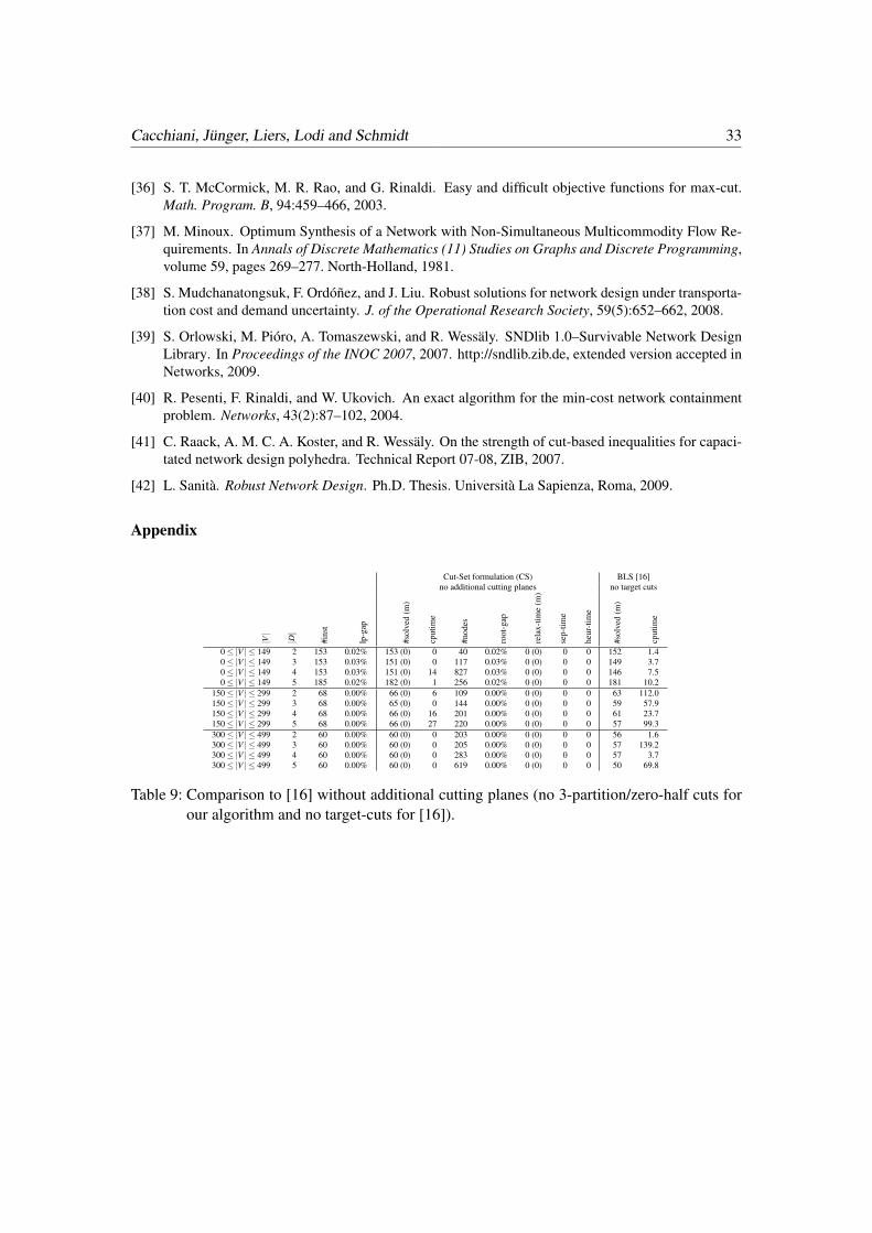
Cacchiani, Jünger, Liers, Lodi and Schmidt 33
[36] S. T. McCormick, M. R. Rao, and G. Rinaldi. Easy and difficult objective functions for max-cut.Math. Program. B, 94:459–466, 2003.
[37] M. Minoux. Optimum Synthesis of a Network with Non-Simultaneous Multicommodity Flow Re-quirements. In Annals of Discrete Mathematics (11) Studies on Graphs and Discrete Programming,volume 59, pages 269–277. North-Holland, 1981.
[38] S. Mudchanatongsuk, F. Ordóñez, and J. Liu. Robust solutions for network design under transporta-tion cost and demand uncertainty. J. of the Operational Research Society, 59(5):652–662, 2008.
[39] S. Orlowski, M. Pióro, A. Tomaszewski, and R. Wessäly. SNDlib 1.0–Survivable Network DesignLibrary. In Proceedings of the INOC 2007, 2007. http://sndlib.zib.de, extended version accepted inNetworks, 2009.
[40] R. Pesenti, F. Rinaldi, and W. Ukovich. An exact algorithm for the min-cost network containmentproblem. Networks, 43(2):87–102, 2004.
[41] C. Raack, A. M. C. A. Koster, and R. Wessäly. On the strength of cut-based inequalities for capaci-tated network design polyhedra. Technical Report 07-08, ZIB, 2007.
[42] L. Sanità. Robust Network Design. Ph.D. Thesis. Università La Sapienza, Roma, 2009.
Appendix
Cut-Set formulation (CS) BLS [16]no additional cutting planes no target cuts
|V|
|D|
#ins
t
lp-g
ap
#sol
ved
(m)
cput
ime
#nod
es
root
-gap
rela
x-tim
e(m
)
sep-
time
heur
-tim
e
#sol
ved
(m)
cput
ime
0≤ |V | ≤ 149 2 153 0.02% 153 (0) 0 40 0.02% 0 (0) 0 0 152 1.40≤ |V | ≤ 149 3 153 0.03% 151 (0) 0 117 0.03% 0 (0) 0 0 149 3.70≤ |V | ≤ 149 4 153 0.03% 151 (0) 14 827 0.03% 0 (0) 0 0 146 7.50≤ |V | ≤ 149 5 185 0.02% 182 (0) 1 256 0.02% 0 (0) 0 0 181 10.2
150≤ |V | ≤ 299 2 68 0.00% 66 (0) 6 109 0.00% 0 (0) 0 0 63 112.0150≤ |V | ≤ 299 3 68 0.00% 65 (0) 0 144 0.00% 0 (0) 0 0 59 57.9150≤ |V | ≤ 299 4 68 0.00% 66 (0) 16 201 0.00% 0 (0) 0 0 61 23.7150≤ |V | ≤ 299 5 68 0.00% 66 (0) 27 220 0.00% 0 (0) 0 0 57 99.3300≤ |V | ≤ 499 2 60 0.00% 60 (0) 0 203 0.00% 0 (0) 0 0 56 1.6300≤ |V | ≤ 499 3 60 0.00% 60 (0) 0 205 0.00% 0 (0) 0 0 57 139.2300≤ |V | ≤ 499 4 60 0.00% 60 (0) 0 283 0.00% 0 (0) 0 0 57 3.7300≤ |V | ≤ 499 5 60 0.00% 60 (0) 0 619 0.00% 0 (0) 0 0 50 69.8
Table 9: Comparison to [16] without additional cutting planes (no 3-partition/zero-half cuts forour algorithm and no target-cuts for [16]).

Cacchiani, Jünger, Liers, Lodi and Schmidt 34
Cut-Set formulation (CS), no additional cutting planes Cut-Set formulation with additional cutting planes
|V|
|E|
|D|
lp-g
apin
%
#sol
ved
(m)
cput
ime
#nod
es
root
-gap
in%
rela
x-tim
e(t
)
sep-
time
heur
-tim
e
#sol
ved
(m)
cput
ime
#nod
es
root
-gap
in%
rela
x-tim
e(t
)
sep-
time
heur
-tim
e
50 211 5 6.9 173 ( 7) 113 3042 2.9 0 (0) 14 0 162 ( 18) 154 3778 2.6 0 (0) 11 150 211 10 6.2 152 ( 28) 196 4766 2.8 0 (0) 29 2 137 ( 43) 232 7195 2.4 0 (0) 30 350 211 30 5.2 146 ( 34) 192 3900 2.4 0 (0) 52 5 133 ( 47) 261 6192 2.1 0 (0) 64 850 211 50 4.7 143 ( 37) 167 3083 2.2 0 (0) 61 6 130 ( 50) 318 5954 2.1 0 (0) 96 1350 211 75 4.4 153 ( 27) 92 1672 2.0 0 (0) 46 5 140 ( 40) 281 5177 2.0 0 (0) 115 1650 211 100 4.7 152 ( 28) 58 1099 2.5 0 (0) 33 3 134 ( 46) 292 5316 2.5 0 (0) 135 1560 256 5 6.3 169 ( 11) 165 3272 2.7 0 (0) 20 1 156 ( 24) 327 5876 2.5 0 (0) 21 260 256 10 5.3 133 ( 47) 269 5525 2.4 0 (0) 43 4 107 ( 68) 257 5036 1.7 0 (0) 30 360 256 30 4.5 135 ( 45) 279 4841 2.2 0 (0) 79 9 112 ( 68) 309 5459 1.6 0 (0) 76 960 256 50 3.9 134 ( 46) 154 2409 1.9 0 (0) 61 6 114 ( 66) 350 5105 1.7 0 (0) 109 1460 256 75 3.8 138 ( 42) 103 1623 1.8 0 (0) 52 5 116 ( 64) 293 4154 1.6 0 (0) 110 1360 256 100 4.0 141 ( 39) 24 477 1.5 0 (0) 17 1 117 ( 62) 85 1809 1.5 0 (0) 48 5
Table 10: Comparison: Cut-Set formulation without additional cutting planes (left) versus Cut-Set formulation with 3-partition inequalities (separated with EnumZH) and the zero-half cuts from [5] (right). Up to an instance size of 50 nodes, the algorithms performcomparibly (not shown in the table). The additional cuts become very important af-terwards. We did not compute values for n ∈ {70,80,90,100} because the experimenttakes a significant amount of time (in our hardware setting, we can expect a total exe-cution time of at least one month for the missing rows).
n EnumZH MinCutZH FischettiZH EnumZH+FischettiZH25 12.3 5.2 7.2 12.430 9.1 3.2 3.9 9.235 7.5 2.5 2.7 7.640 10.3 3.7 3.4 10.645 8.0 2.6 1.9 8.150 9.4 2.9 3.3 9.4
Table 11: Root bound improvement in percent. Instances from the JMP class.


![[Commodity Name] Commodity Strategy](https://static.fdocuments.net/doc/165x107/568135d2550346895d9d3881/commodity-name-commodity-strategy.jpg)


