Single and Multi-CPU Performance Modeling for Embedded Systems · Electrical Engineering and...
191
Single and Multi-CPU Performance Modeling for Embedded Systems Trevor Conrad Meyerowitz Electrical Engineering and Computer Sciences University of California at Berkeley Technical Report No. UCB/EECS-2008-36 http://www.eecs.berkeley.edu/Pubs/TechRpts/2008/EECS-2008-36.html April 14, 2008
Transcript of Single and Multi-CPU Performance Modeling for Embedded Systems · Electrical Engineering and...

Single and Multi-CPU Performance Modeling forEmbedded Systems
Trevor Conrad Meyerowitz
Electrical Engineering and Computer SciencesUniversity of California at Berkeley
Technical Report No. UCB/EECS-2008-36
http://www.eecs.berkeley.edu/Pubs/TechRpts/2008/EECS-2008-36.html
April 14, 2008

Copyright © 2008, by the author(s).All rights reserved.
Permission to make digital or hard copies of all or part of this work forpersonal or classroom use is granted without fee provided that copies arenot made or distributed for profit or commercial advantage and that copiesbear this notice and the full citation on the first page. To copy otherwise, torepublish, to post on servers or to redistribute to lists, requires prior specificpermission.
Single and Multi-CPU Performance Modeling for Embedded Systems
by
Trevor Conrad Meyerowitz
B.S. (Carnegie Mellon University) 1999M.S. (University of California at Berkeley) 2002
A dissertation submitted in partial satisfaction of therequirements for the degree of
Doctor of Philosophy
in
Engineering - Electrical Engineering and Computer Sciences
in the
GRADUATE DIVISIONof the
UNIVERSITY OF CALIFORNIA, BERKELEY
Committee in charge:Professor Alberto Sangiovanni-Vincentelli, Chair
Professor Rastislav BodikProfessor Alper Atamturk
Spring 2008

1
Abstract
Single and Multi-CPU Performance Modeling for Embedded Systems
by
Trevor Conrad Meyerowitz
Doctor of Philosophy in Engineering - Electrical Engineering and Computer
Sciences
University of California, Berkeley
Professor Alberto Sangiovanni-Vincentelli, Chair
The combination of increasing design complexity, increasing concurrency, grow-
ing heterogeneity, and decreasing time to market windows has caused a crisis for
embedded system developers. To deal with this problem, dedicated hardware is
being replaced by a growing number of microprocessors in these systems, making
software a dominant factor in design time and cost. The use of higher level mod-
els for design space exploration and early software development is critical. Much
progress has been made on increasing the speed of cycle-level simulators for mi-
croprocessors, but they may still be too slow for large scale systems and are too
low-level (i.e. they require a detailed implementation) for effective design space
exploration. Furthermore, constructing such optimized simulators is a significant
task because the particularities of the hardware must be accounted for. For this
reason, these simulators are hardly flexible.
This thesis focuses on modeling the performance of software executing on em-
bedded processors in the context of a heterogeneous multi-processor system on
chip in a more flexible and scalable manner than current approaches. We contend
that such systems need to be modeled at a higher level of abstraction and, to ensure accu-
racy, the higher level must have a connection to lower-levels. First, we describe different

2
levels of abstraction for modeling such systems and how their speed and accuracy
relate. Next, the high-level modeling of both individual processing elements and
also a bus-based microprocessor system are presented. Finally, an approach for au-
tomatically annotating timing information obtained from a cycle-level model back
to the original application source code is developed. The annotated source code
can then be simulated without the underlying architecture and still maintain good
timing accuracy. These methods are driven by execution traces produced by lower
level models and were developed for ARM microprocessors and MuSIC, a hetero-
geneous multiprocessor for Software Defined Radio from Infineon. The annotated
source code executed between one to three orders of magnitude faster than equiv-
alent cycle-level models, with good accuracy for most applications tested.
Professor Alberto Sangiovanni-VincentelliDissertation Committee Chair

i
To my family.

ii
Contents
1 Introduction 11.1 Traditional Embedded System Design . . . . . . . . . . . . . . . . . . 2
1.1.1 Traditional Hardware Development Flow . . . . . . . . . . . . 21.1.2 Traditional Software Development Flow . . . . . . . . . . . . 41.1.3 Problems with the Traditional Flow . . . . . . . . . . . . . . . 4
1.2 Motivating Trends for System Level Design . . . . . . . . . . . . . . . 51.2.1 Complexity and Productivity . . . . . . . . . . . . . . . . . . . 51.2.2 Multicore Processors . . . . . . . . . . . . . . . . . . . . . . . . 61.2.3 Explosion of Software and Programmability . . . . . . . . . . 8
1.3 System-Level Design . . . . . . . . . . . . . . . . . . . . . . . . . . . . 91.3.1 The Y-Chart and Separation of Concerns . . . . . . . . . . . . 91.3.2 Platform Based Design . . . . . . . . . . . . . . . . . . . . . . . 111.3.3 Models of Computation . . . . . . . . . . . . . . . . . . . . . . 131.3.4 System Level Design Flows . . . . . . . . . . . . . . . . . . . . 171.3.5 Transaction Level Modeling . . . . . . . . . . . . . . . . . . . . 191.3.6 Metropolis . . . . . . . . . . . . . . . . . . . . . . . . . . . . . . 21
1.4 Levels for Modeling Embedded Software . . . . . . . . . . . . . . . . 291.4.1 Computer Architecture Simulation Technologies . . . . . . . . 311.4.2 Processor Simulation Technologies for Embedded Systems . 32
1.5 Discussion . . . . . . . . . . . . . . . . . . . . . . . . . . . . . . . . . . 341.6 Contributions and Outline . . . . . . . . . . . . . . . . . . . . . . . . . 35
2 Single Processor Modeling 372.1 Processor Modeling Definitions . . . . . . . . . . . . . . . . . . . . . . 38
2.1.1 Functional Definitions . . . . . . . . . . . . . . . . . . . . . . . 382.1.2 Architectural Definitions . . . . . . . . . . . . . . . . . . . . . . 41
2.2 Processor Models . . . . . . . . . . . . . . . . . . . . . . . . . . . . . . 472.2.1 High Level Overview . . . . . . . . . . . . . . . . . . . . . . . 472.2.2 Trace Format . . . . . . . . . . . . . . . . . . . . . . . . . . . . 50

iii
2.2.3 Adding a Memory System to the Models . . . . . . . . . . . . 512.2.4 Model Limitations . . . . . . . . . . . . . . . . . . . . . . . . . 54
2.3 Case Study and Results . . . . . . . . . . . . . . . . . . . . . . . . . . . 542.3.1 XScale and Strongarm Processors . . . . . . . . . . . . . . . . . 552.3.2 Accuracy Results . . . . . . . . . . . . . . . . . . . . . . . . . . 552.3.3 Performance Results and Optimizations . . . . . . . . . . . . . 58
2.4 Related Work . . . . . . . . . . . . . . . . . . . . . . . . . . . . . . . . 612.5 Discussion . . . . . . . . . . . . . . . . . . . . . . . . . . . . . . . . . . 63
3 Multiprocessor Modeling 643.1 Introduction . . . . . . . . . . . . . . . . . . . . . . . . . . . . . . . . . 66
3.1.1 Software Defined Radio . . . . . . . . . . . . . . . . . . . . . . 663.1.2 the MuSIC Multiprocessor for Software Defined Radio . . . . 673.1.3 Prior Architectural Models in Metropolis . . . . . . . . . . . . 68
3.2 Architectural Modeling . . . . . . . . . . . . . . . . . . . . . . . . . . . 723.2.1 Modeling Computation and Communication . . . . . . . . . 723.2.2 Modeling Cost and Scheduling . . . . . . . . . . . . . . . . . . 763.2.3 Modeling the MuSIC Architecture . . . . . . . . . . . . . . . . 79
3.3 Modeling Functionality and Mapping . . . . . . . . . . . . . . . . . . 833.3.1 Functionality . . . . . . . . . . . . . . . . . . . . . . . . . . . . 833.3.2 Mapping . . . . . . . . . . . . . . . . . . . . . . . . . . . . . . . 85
3.4 Results . . . . . . . . . . . . . . . . . . . . . . . . . . . . . . . . . . . . 883.4.1 Modeling Code Complexity . . . . . . . . . . . . . . . . . . . . 883.4.2 Architecture Netlist Statistics . . . . . . . . . . . . . . . . . . . 89
3.5 Discussion . . . . . . . . . . . . . . . . . . . . . . . . . . . . . . . . . . 91
4 Introduction to Timing Annotation 944.1 Basic Information . . . . . . . . . . . . . . . . . . . . . . . . . . . . . . 95
4.1.1 What is Annotation? . . . . . . . . . . . . . . . . . . . . . . . . 954.1.2 Tool Flow . . . . . . . . . . . . . . . . . . . . . . . . . . . . . . 954.1.3 Basic Definitions . . . . . . . . . . . . . . . . . . . . . . . . . . 98
4.2 Annotation Platforms . . . . . . . . . . . . . . . . . . . . . . . . . . . . 994.2.1 MuSIC Multiprocessor for Software Defined Radio . . . . . . 1014.2.2 The XScale Microprocessor . . . . . . . . . . . . . . . . . . . . 102
4.3 Related Work . . . . . . . . . . . . . . . . . . . . . . . . . . . . . . . . 1034.3.1 Software Tools . . . . . . . . . . . . . . . . . . . . . . . . . . . . 1034.3.2 Performance Estimation for Embedded Systems . . . . . . . . 1044.3.3 Worst-Case Execution Time Analysis . . . . . . . . . . . . . . . 1064.3.4 Other Work . . . . . . . . . . . . . . . . . . . . . . . . . . . . . 107
4.4 Discussion . . . . . . . . . . . . . . . . . . . . . . . . . . . . . . . . . . 107

iv
5 Backwards Timing Annotation for Uniprocessors 1085.1 Single Processor Timing Annotation Algorithm . . . . . . . . . . . . . 108
5.1.1 Construct Blocks and Lines . . . . . . . . . . . . . . . . . . . . 1095.1.2 Calculate Block and Line-Level Annotations . . . . . . . . . . 1125.1.3 Generating Annotated Source Code . . . . . . . . . . . . . . . 113
5.2 Implementation and Optimizations . . . . . . . . . . . . . . . . . . . . 1165.2.1 Memory Usage Optimizations . . . . . . . . . . . . . . . . . . 1175.2.2 Trace Storage Optimizations . . . . . . . . . . . . . . . . . . . 119
5.3 Uniprocessor Annotation Results . . . . . . . . . . . . . . . . . . . . . 1215.3.1 Simulation Platforms Evaluated . . . . . . . . . . . . . . . . . 1215.3.2 Results with Identical Data . . . . . . . . . . . . . . . . . . . . 1225.3.3 Results with Different Data . . . . . . . . . . . . . . . . . . . . 1295.3.4 Annotation Framework Runtime . . . . . . . . . . . . . . . . . 1315.3.5 Analysis . . . . . . . . . . . . . . . . . . . . . . . . . . . . . . . 134
5.4 Discussion . . . . . . . . . . . . . . . . . . . . . . . . . . . . . . . . . . 136
6 Backwards Timing Annotation for Multiprocessors 1376.1 Introduction . . . . . . . . . . . . . . . . . . . . . . . . . . . . . . . . . 138
6.1.1 Motivating Example . . . . . . . . . . . . . . . . . . . . . . . . 1386.2 Handling Startup Delays . . . . . . . . . . . . . . . . . . . . . . . . . . 1396.3 Handling Inter-Processor Communication . . . . . . . . . . . . . . . . 143
6.3.1 Example with Inter-processor Communication Problems . . . 1436.3.2 Ignoring Inter-processor Communication Delays . . . . . . . . 1436.3.3 Characterizing Inter-Thread Operations . . . . . . . . . . . . . 1446.3.4 Handling Pipelining . . . . . . . . . . . . . . . . . . . . . . . . 1456.3.5 Why not analyze all of the processors concurrently? . . . . . . 146
6.4 Results and Analysis . . . . . . . . . . . . . . . . . . . . . . . . . . . . 1486.4.1 Results with Identical Data . . . . . . . . . . . . . . . . . . . . 1496.4.2 Results with Different Data . . . . . . . . . . . . . . . . . . . . 1506.4.3 Analysis . . . . . . . . . . . . . . . . . . . . . . . . . . . . . . . 152
6.5 Discussion . . . . . . . . . . . . . . . . . . . . . . . . . . . . . . . . . . 1536.5.1 Limitations . . . . . . . . . . . . . . . . . . . . . . . . . . . . . 153
7 Conclusions 1557.1 Future Work . . . . . . . . . . . . . . . . . . . . . . . . . . . . . . . . . 156
7.1.1 Modeling . . . . . . . . . . . . . . . . . . . . . . . . . . . . . . 1567.1.2 Annotation . . . . . . . . . . . . . . . . . . . . . . . . . . . . . 157
7.2 Discussion . . . . . . . . . . . . . . . . . . . . . . . . . . . . . . . . . . 159
Bibliography 162
v
Acknowledgments
First off I would like to thank my advisor, Professor Sangiovanni-Vincentelli, for
his guidance, support, insight, and patience over the years. I also want to thank
Professors Atamturk and Bodik for being the other readers of my dissertation and
for providing helpful feedback. I also want to thank the other professors on my
qualifying exam committee: Professors Atamturk, Keutzer, and Patterson.
A huge amount of thanks and gratitude goes to my great friend David Chin-
nery, who carefully proofread each of these chapters at some stage of development,
gave tough and helpful feedback, and also provided a huge amount of support
throughout this process. Alessandro Pinto read parts of this thesis, and provided
useful feedback, especially on an early version of the processor definitions. While
not touching it directly, Julius Kusuma, has been an excellent friend and taskmas-
ter who pushed me forward at different stages while providing encouragement
and not-so softly forced me into the cult of LaTex, which I now totally appreciate.
Qi Zhu and Haibo Zheng also provided feedback on individual chapters.
I must acknowledge all of the people have participated in this work. Kees Vis-
sers provided the initial idea of using Kahn Process Networks for processor mod-
eling, and Sam Williams with whom the initial work was done. Qi Zhu and Haibo
Zeng made an extension of the models to a superscalar model. Min Chen exam-
ined quasi-static scheduling of the processor models. The multiprocessor mod-
eling was based upon the work of Rong Chen, was done in collaboration with
Jens Harnisch from Infineon. Abhijit Davare and Qi Zhu provided assistance with
mapping and quantity managers in Metropolis. Mike Kishinevsky and Timothy
Kam at intel were the industrial liasons for the uniprocessor modeling work. The
annotation work was done in collaboration with Mirko Sauermann and Dominik
Langen at Infineon. Useful discussions and background support was provided by
other members of the MuSIC SDR team at Infineon including: Cyprian Grassman,
Ulrich Hachman, Wolfgang Raab, Ulrich Ramacher, Matthias Richter, and Alfonso
Troya.
vi
I also want to highlight the excellent officemates that I’ve had: Luca Carloni
(Papa Carloni and Clash Expert), Satrajit ‘Sat’ Chatterjee (Programming and LTris
Guru), Philip Chong, Shauki Elassaad, Yanmei Li, and Fan Mo.
A number of people have had special impact on my graduate experience, and
I list them here. Ruth Gjerde and Mary Byrnes were always there for support
and guidance through the bureaucracy and the general struggles with graduate
school. Luciano Lavagno was the first person I met when visiting Berkeley, and
was always quick to respond with thoughtful and friendly feedback. Jonathan
Sprinkle’s model integrated computing class was most interesting. The FLEET
class run by Ivan Sutherland and Igor Benko, was inspiring and challenging. Pro-
fessor Kristofer Pister provided moral support and advice at a critical juncture.
I’ve had the pleasure to get to know a number of classmates, instructors, men-
tors, visitors, and friends while at Berkeley. They have enhanced the experience
with their friendliness, kindness, humor, and intelligence. These include, but
are not limited to: Alvise Bonivento, Bryan Brady, Robert Brayton, Christopher
Brooks, Mireille Broucke, Luca Carloni, Mike Case, Adam Cataldo, Bryan Catan-
zaro, Donald Chai, Arindam Chakrabarti, Satrajit ‘Sat’ Chatterjee, Rong Chen, Xi
Chen, David Chinnery, Jike Chong, Massimiliano D’Angelo, Abhijit Davare, Fer-
nando De Bernardinis, Douglas Densmore, Carlo Fischione, Arkadeb Ghosal, Gre-
gor Goessler, Matthias Gries, Yujia Jin, Vinay Krishnan, Animesh Kumar, William
Jiang, Edward Lee, Yanmei Li, Cong Liu, Kelvin Lwin, Slobodan Matic, Emanuele
Mazzi, Mark McKelvin, Andrew Mihal, Fan Mo, John Moondanos, Matthew Mosk-
ewicz, Alessandra Nardi, Luigi Palopoli, Roberto Passerone, Hiren Patel, Clau-
dio Pinello, Alessandro Pinto, William Plishker, Kaushik Ravindran, N.R. Satish,
Christian Sauer, Marco Sgroi, Vishal Shah, Niraj Shah, Farhana Sheikh, Alena
Samalatsar, Mary Stewart, Xuening Sun, Martin Trautmann, Gerald Wang, Yoshi
Watanabe, Scott Weber, James Wu, Guang Yang, Yang Yang, Stefano Zanella, Haibo
Zeng, Wei Zheng, and Qi Zhu. To anyone I left out: I apologize, and it was not in-
tentional.

vii
There have been a number talented and friendly administrators that have kept
me paid and sane over the years, they include: Jennifer Stone, Dan MacLeod,
and Jontae Gray, Lorie Mariano (BOOO!!), Gladys Khoury, Flora Oviedo, Nuala
Mattherson, and Mary-Margaret Sprinkle.
Computer support (and salvage) was provided by Brad Krebs, Marvin Motley,
and Phil Loarie. More than once did they save me from failed hardware, crashed
software, or my own mistakes.
I want to thank my parents and sister for their love, advice, and support through-
out this process. I also want to thank my grandparents for their love, for helping
me keep perspective, and for not asking “When again are you planning to finish?”
too often.
I also want to acknowledge a number of great friends that I’ve had outside of
the department who have helped me relax and reconnect with the real world. They
include: Carolina Armenteros, Ryan and Andrew Duryea, Tamara Freeze, Daniel
Hay, Lee Istrail, Ying Liu, Robin Loh, Dave Lockner, Cris Luengo, John and Ang
Montoya, Eleyda Negron, Pavel Okunev, Farah Sanders, and Mel Schramek. I am
sorry if I missed anybody on this list.
This research was funded from a number of sources including: SRC custom
funding from Intel, Infineon Corporation, the Gigascale Systems Research Center,
and the Center for Hybrid and Embedded Systems Software. CoWare donated
software licenses that enabled the annotation work, once a contract was negotiated
with the help of Eric Giegerich.

1
Chapter 1
Introduction
Embedded literally means ‘within’, so an embedded system is a system within
another system. An embedded system is a system that interacts with the real world.
Typically it reads inputs from sensors, performs some computation, and then out-
puts data via actuators. Examples of embedded systems include: cellphones, auto-
motive controls, wireless sensor networks, power plant controls, and mp3 players.
Embedded applications are constrained in ways that normal computer applica-
tions are not: many of them have realtime deadlines that must be met, and factors
such as power usage and system cost are of paramount concern.
This chapter begins by reviewing the traditional design flow for embedded sys-
tem design, including a discussion of why it is insufficient for today’s designs.
Then, Section 1.2 presents motivating trends pushing us towards using system
level design. After this, Section 1.3 reviews key elements of system level design in-
cluding platform-based design, transaction-level modeling and also a description
of the Metropolis system-level design framework. Section 1.4 presents different
levels of abstraction for modeling the performance of software running on an em-
bedded processor, which is critical for putting our work into context. Finally, the
contributions and ordering of this thesis are presented.
2
Register Transfer Level Models
Logic Gates
Layout
Algorithmic Models
Transaction-Level Models
Actual Gates
Abstract
Detailed
Specification
Implementation
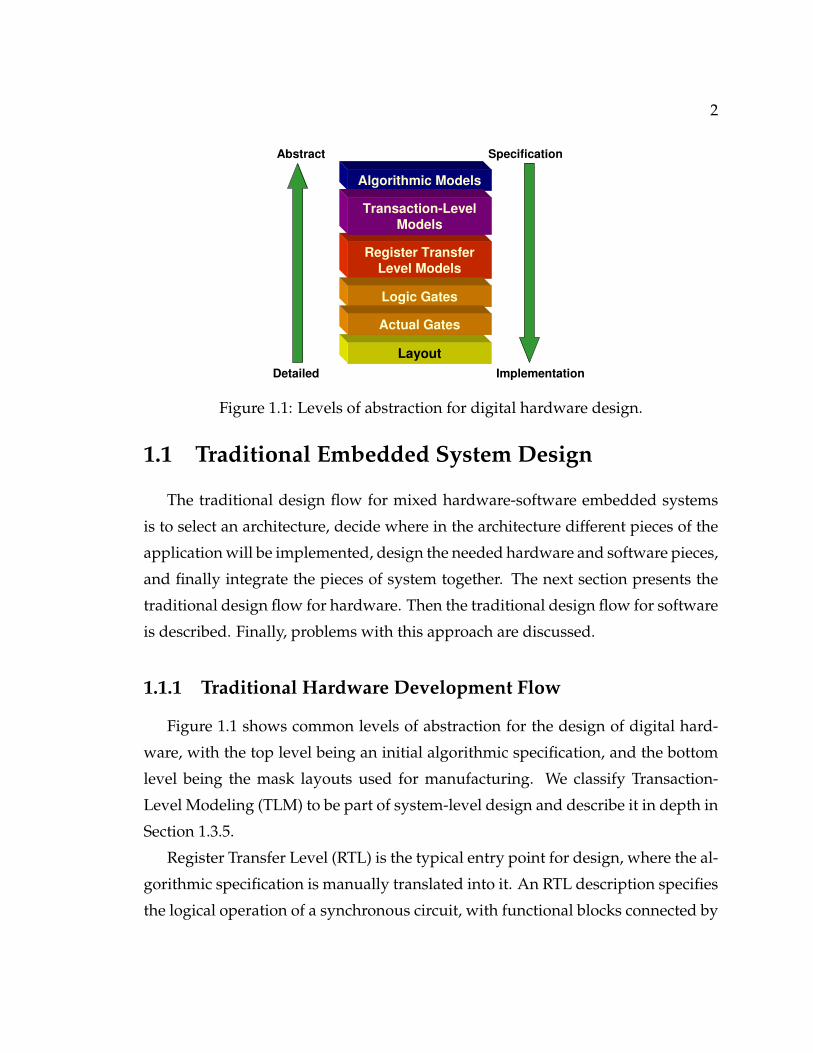
Figure 1.1: Levels of abstraction for digital hardware design.
1.1 Traditional Embedded System Design
The traditional design flow for mixed hardware-software embedded systems
is to select an architecture, decide where in the architecture different pieces of the
application will be implemented, design the needed hardware and software pieces,
and finally integrate the pieces of system together. The next section presents the
traditional design flow for hardware. Then the traditional design flow for software
is described. Finally, problems with this approach are discussed.
1.1.1 Traditional Hardware Development Flow
Figure 1.1 shows common levels of abstraction for the design of digital hard-
ware, with the top level being an initial algorithmic specification, and the bottom
level being the mask layouts used for manufacturing. We classify Transaction-
Level Modeling (TLM) to be part of system-level design and describe it in depth in
Section 1.3.5.
Register Transfer Level (RTL) is the typical entry point for design, where the al-
gorithmic specification is manually translated into it. An RTL description specifies
the logical operation of a synchronous circuit, with functional blocks connected by

3
wires and registers. Verilog and VHDL are common Hardware Description Lan-
guages (HDLs) used for specifying designs at RTL-level.
HDLs have a synthesizable subset that can be automatically translated into lay-
out via the following design flow. The first step is to perform technology indepen-
dent optimizations on the HDL netlist to generate an optimized logical netlist con-
sisting of AND-gates, inverters, and registers. After this, technology dependent
optimization maps the logical netlist onto a set of actual gates that will be imple-
mented as layout. From here the actual gates are placed and connected via wire
routing. [111] and [61] provide more detailed description of the logic synthesis
flow.
A key element of the different levels of abstraction in the hardware design flow
is how fast they can be simulated, and at what level of accuracy. An algorithmic
model is native code running on the host, which is fast, but has no notion of the
implementation’s performance. Transaction-level models (TLM) feature concur-
rent blocks communicating via function calls to high-level channels; depending on
their level of detail TLM models have a wide range of speed and accuracy. RTL
simulation is performed at the level of individual signals and gates, making it sig-
nificantly slower than the algorithmic and TLM levels. Pieces of the layout-level
are simulated at the circuit-level, and these results (e.g. parasitic capacitance and
noise) are annotated back to the gate level netlists. Going to a higher level of ab-
straction usually results in at least an order of magnitude (and often two or more)
increase in simulation speed.
For different design and verification tasks it is critical to understand what in-
formation is needed and then pick the appropriate level(s) of abstraction to ac-
complish this. For example, there is no point in simulating application software
running processor with transistor-level SPICE models, because it would be far too
slow. We are concerned with RTL and higher level models in this dissertation and
will not mention the lower levels from hereafter.

4
1.1.2 Traditional Software Development Flow
Software development in the traditional design flow for embedded systems can
be broken into two phases: hardware-independent development and hardware-
dependent development. Hardware-independent development involves imple-
menting the pieces of the system that do not directly depend on the underlying
hardware and either ignoring the hardware, or representing it with software stubs
used as placeholders. Often significant pieces of the algorithmic models can be
reused as hardware-independent software, as these models are typically written
in C or C++.
Hardware-dependent software development involves interfacing the software
with the hardware in the system, and also optimizing the software to meet per-
formance constraints. The interfacing of hardware and software is an error prone
and time consuming process that involves using features such as interrupts, real-
time operating systems, and memory-mapped communication. This can only be-
gin when there is a model of the hardware of sufficient detail available. For pre-
existing hardware platforms this is not a problem, but it can be when new plat-
forms are being developed. Often the hardware model is the RTL-level model,
and so it is not ready until late in the design cycle, which can significantly extend
overall development time. Furthermore, co-simulating software running on pro-
cessor models with HDLs can be quite slow. Finally, in order to meet performance
requirements, low-level programming at the assembly level is frequently needed.
Different levels of abstraction for modeling microprocessors are detailed in Section
1.4.
1.1.3 Problems with the Traditional Flow
There are several problems with the traditional approach for designing mixed
hardware-software embedded systems. Since the implementation is done at a low
level it is difficult to change the mapping, or to reuse pieces of the application. If

5
an inadequate system architecture is selected, it will often not be discovered until
late into the design process, and thus can cause great delays. Architects sometimes
compensate for this risk by over-building the system, but this increases the cost of
the system. Also, the lack of formal underpinning of the implementation makes
it difficult, if not impossible, to fully verify such designs. Finally, the disconnect
between the hardware and software design teams can lead to incompatibilities that
only arise at the integration stage. All of these problems are growing as embedded
systems continue to increase in complexity.
1.2 Motivating Trends for System Level Design
As previously discussed, the traditional design flow for embedded systems is
not scaling. This section reviews such trends, all of which point to the need for
higher level design and modeling.
1.2.1 Complexity and Productivity
Moore’s law, illustrated in Figure 1.2, states that the number of transistors on a
chip doubles roughly every 18 months. This must be put to a good competitive ad-
vantage to improve in one or more of the following areas: speed, power, cost, and
the expansion of capabilities. A key challenge of Electronic Design Automation
(EDA) is to help designers keep pace with Moore’s law.
In 1999 the International Technology Roadmap for Semiconductors (ITRS) es-
timated [5] that design complexity is growing at 58% rate, whereas designer pro-
ductivity is only growing at a rate of only 21%. This gap is referred to a the ‘design
productivity gap’. Two key ways of closing this gap are design reuse and doing
design at a higher level of abstraction.
In 1999 Shekhar Borkar of Intel estimated [33] that, were the current power and
frequency scaling trends to continue, the power consumption of a microprocessor

6
Figure 1.2: Moore’s Law illustrated through the transistor count of Intel processorsover time. (Copyright c©2004 Intel Corporation.)
would reach the unsustainable level of 2,000W in the year 2010. In order to avoid
this, processor frequencies actually dropped as Intel moved to less aggressively
pipelined multicore designs; a high-profile example of this was Intel canceling the
Pentium 4 Tejas microprocessor and moving to more efficient dual processors be-
cause of power concerns [66]. Another way to continue Moore’s law without ex-
ceeding power constraints is to use more cores on a chip that are less complicated
than today’s processors. In 2007, Borkar [32] advocated putting hundreds, if not
thousands, of simpler cores on a single chip to scale performance while staying
within the power budget.
1.2.2 Multicore Processors
Many domains are already multicore or multiprocessor, and this trend is only
increasing due to power and performance concerns [24]. The major microproces-
sor producing companies for general purpose and server computing (such as Intel,

7
AMD, Sun, and IBM) all have produced multicore designs for their mainstream
products. In 2007, Intel presented a prototype of an 80 core network on chip run-
ning at up to 4 GHz [142] fabricated in 65nm bulk CMOS. This achieved up to
1.28 TFLOPS of performance, while consuming 181 W of power. By reducing the
voltage by half the chip used 18x less power and was 4x slower. This illustrates
what is currently possible with recent semiconductor technology, and also what
the challenges are; specifically, raising voltage to increase performance is far less
effective than replicating functionality and exploiting parallelism.
In some domains, multiprocessing is already prevalent. Most cellphones today
have a RISC control processor and a DSP processor, with higher end models having
additional processors dedicated to handling demanding multimedia applications
like digital video decoding. Networking applications consist of tasks (e.g. packet
routing) that need to be done quickly and have a large amount of parallelism (e.g.
at the packet level). In 2001, Intel released the IXP1200 [49], which features a single
Strongarm processor along with 6 packet processing microengines. Intel’s latest
network processor (as of February 2008), the IXP2800 [50], has an XScale processor
and 16 packet processing engines along with hardware acceleration for encryp-
tion for performing secure packet routing at up to 1010 packets per second. In
2005, Cisco Systems presented the Metro NP network processor [17]. It features
188 XTensa 32-bit RISC processors with extensions for network processing and a
peak performance of 7.8 × 10⁷ packets per second. It achieves all of this perfor-
mance while only consuming 35 watts of power. Some of the current generation of
gaming consoles also feature multiprocessors. The Cell Broadband Engine [70, 71]
was released in 2006 and powers the Playstation 3 gaming console, servers, super-
computers, and there are plans to add it to consumer-electronics devices, such as
high-definition televisions. The Cell is a heterogeneous multiprocessor featuring
a single traditional microprocessor implementing the Power architecture [9] along
with up to 8 Synegistic Processing Elements (SPEs) connected via a high speed
communication system. Each SPE contains local memory, a high speed memory

8
controller, and a processing element used for high-speed data-parallel computa-
tions. The Xbox360 [22] is also multiprocessor with a core containing three multi-
threaded processors implementing the Power architecture.
1.2.3 Explosion of Software and Programmability
In 2003, Intel’s director of design technology Greg Spirakis estimated software
development to be 80% of the development cost for embedded systems, and said
that the speed of high level modeling for architectural exploration and hardware
software co-design are key concerns [138]. In 2004, Hans Frischorn of BMW (and
now at General Motors) [68] said that 40% of the cost of automobiles is now at-
tributed to electronics and software, where 50% to 70% of this cost is for software
development. Frischorn also said that up to 90% of future vehicle innovations will
be due to electronics and software, and that premium automobiles can have up to
70 Electronic Control Units (ECUs) communicating over five system buses. Fur-
thermore, automotive systems especially challenging because they are distributed
and many have hard real time deadlines.
Programming embedded multiprocessor systems is difficult. They are gener-
ally programmed at a relatively low level using C, C++, or even assembly lan-
guage. The concurrency in these systems is often handled by using multi-threading
libraries. In [94], Lee highlights some of the productivity and reliability issues of
programming parallel systems with threads. He advocates the use of more intu-
itive and analyzable models of computation for concurrent modeling. Recently,
there has been major research funding the exploration of new programming mod-
els for multiprocessor systems [106].
In addition to concurrency, the size of software in such systems is rapidly ex-
panding. Sangiovanni-Vincentelli [135] states that, “In cell phones, more than 1
million lines of code is standard today, while in automobiles the estimated num-
ber of lines by 2010 is in the order of hundreds of millions. The number of lines
of source code of embedded software required for defense avionics systems is also
9
growing exponentially...”. To cope with all of these challenges it is critical to have:
fast and accurate simulation, well defined levels of abstraction, and effective tools
for system analysis and optimization.
1.3 System-Level Design
Whereas the traditional design flow is directly aimed at implementation,
system-level design [103, 135] uses abstract models that can be quickly be changed
in terms of structure, parameters, and components. These higher-level abstractions
enable the exploration of a larger design-space and generally lead superior imple-
mentations. Furthermore, these abstractions often have formal underpinnings and
so can enable verification and synthesis. Key elements of system level design in-
clude: abstract specification, high-level synthesis, and virtual prototyping.
This section first reviews key concepts for system-level design, which include:
the Y-chart, separation of concerns, and models of computation. Then, previous
work in system-level design environments is explained. Section 1.3.5 details trans-
action level modeling. Finally, Section 1.3.6 reviews the Metropolis system level
design framework.
1.3.1 The Y-Chart and Separation of Concerns
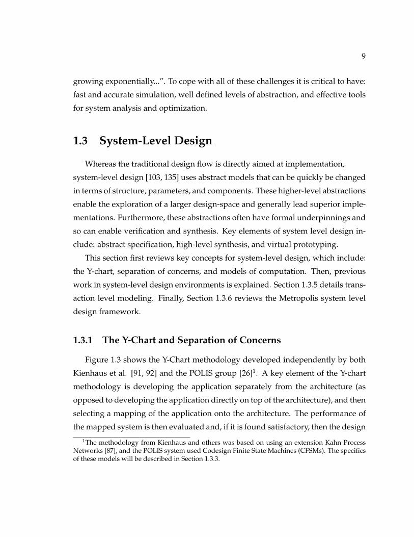
Figure 1.3 shows the Y-Chart methodology developed independently by both
Kienhaus et al. [91, 92] and the POLIS group [26]1. A key element of the Y-chart
methodology is developing the application separately from the architecture (as
opposed to developing the application directly on top of the architecture), and then
selecting a mapping of the application onto the architecture. The performance of
the mapped system is then evaluated and, if it is found satisfactory, then the design
1The methodology from Kienhaus and others was based on using an extension Kahn ProcessNetworks [87], and the POLIS system used Codesign Finite State Machines (CFSMs). The specificsof these models will be described in Section 1.3.3.
10
Application Architecture
Mapping
Performance
AnalysisModify
Application
Modify
Architecture
Modify
Mapping
Figure 1.3: An overview of the Y-Chart methodology. The application and archi-tecture are designed, and then a mapping from the application to the architectureis specified. After this performance analysis is performed. If the design criteria arenot met, the functionality, architecture, and mapping can be modified.
11
is finished. If performance needs to be improved then three different elements can
be modified, the application, the architecture, and the mapping of the application
onto the architecture. By keeping these elements separated, reuse is improved and
the opportunities for design space exploration are expanded.
The Y-chart methodology keeps the architecture, application, and mapping sep-
arated. Keutzer et al. extended [90] this idea to include a number of other aspects.
Communication and computation have been separated, which is a key element
of transaction level modeling (detailed in Section 1.3.5). Another important piece
is the separation between behavior and performance. By keeping these elements
separated reuse and analyzability are increased.
1.3.2 Platform Based Design
The notion of platforms is widely used in industry. One popular view of a plat-
form is that it is a set of configurable and compatible components. This might in-
clude a family of different microprocessors that all implement the same instruction
set at various levels of cost and performance, or it might extend to include a full
system along with hardware and software. Thus, if a company develops a product
on a particular platform it can be ensured software compatibility, increased per-
formance, and expanded capabilities in future implementations of this platform.
While intuitive, this definition is quite vague.
In [134], Professor Alberto Sangiovanni-Vincentelli (ASV) formalizes the notion
of platform based design in terms of an application’s functionality and the archi-
tecture that can implement this functionality. Figure 1.4(a) shows the ASV-triangles
that form the basis of Sangiovanni-Vincentelli’s framework. The top triangle rep-
resents the functional space, where a particular function instance is mapped to a
system-platform. The bottom triangle represents the architectural space where a par-
ticular instance of an architecture is created and then exported up to the system
platform. The system platform is where the functional instance interacts with the ar-
chitecture platform using a common set of primitives and other information pro-

12
PlatformDesign-Space
Export
PlatformMapping
Architectural Space
Functional Space
Function Instance
Platform Instance
System Platform
(a) ASV Triangles One Level
Platform 1
Platform 2
Platform 3
…
(b) Multiple Levels of ASV Triangles
Figure 1.4: ASV(Alberto Sangiovanni-Vincentelli)-Triangles for Platform-BasedDesign, shown in as single level and also as a flow with of multiple levels. (Source:Alberto Sangiovanni-Vincentelli)
vided by the platform.
Many design flows and views can be represented in terms of platform-based
design. For a desktop computer the platform might be the x86 instruction set, the
architectural space is the set of processors implementing the instruction set, and
the functional instance would be a C-program connected to libraries targeting the
x86 instruction set. The platform mapping is the compilation of the C-code into
x86 binaries. The platform design-space export might give the compiler a picture
of the microarchitectural implementation of the processor so that it can generate
more efficient binaries (e.g. so as to avoid pipeline stalls or use particular .
In order to provide reasonable design methodology the platforms must be de-
fined so that there is not too large of a gap between the semantics of the functional
space, the system platform, and the architectural space. For example, moving di-

13
rectly from a high level sequential specification to a hardware implementation has
such a large design space and semantic gap that it is difficult to find a ‘good’ result.
Most successful methodologies are broken into multiple levels, where user input
may occur at each level. Figure 1.4(b) shows an example of multiple levels being
used in platform based design. The RTL-synthesis process described in Section
1.1.1 fits well into this flow, with each step being viewed as a platform (i.e. RTL,
boolean algebra, gate-level netlist, and layout).
1.3.3 Models of Computation
A Model of Computation (MOC) is a formal representation of the semantics
of a system. In particular, it define rules on how a set of connected components
execute and interact. Based on the rules of the MOC, its connected components
can be analyzed, simulated, synthesized, or verified to varying degrees of success.
There is a tradeoff between how expressive an MOC is, and how analyzable it
is. For some domains the limits on expressiveness is helpful. Below we review
popular models of computation with an emphasis on those used in this thesis.
1.3.3.1 Finite State Machines
Finite State Machines (FSMs) are a classical model of computation often used
for hardware design. An FSM operates on a set of Boolean inputs and a set Boolean
values indicating the machine’s current state. Based on these, it calculates the next
state of the machine as well as the values of the machine’s outputs. Finite State Ma-
chines map directly into Boolean logic, which makes them easily synthesizeable,
and they are very good for representing control-dominated systems. They are also
amenable to many formal verification techniques [63]. A single FSM is sequen-
tial. FSMs become much more useful (and challenging) when they are combined
together.
There are many extensions to FSMs such as adding: concurrency, hierarchy, and
14
timing. One of the most influential extensions was Statecharts [76], it provided a
visual language that added hierarchy, concurrency, and non-determinism to FSMs.
The Polis [26] project introduced Codesign Finite State Machines (CFSMs), which
are event triggered FSMs communicating via single buffered over-writable chan-
nels.
1.3.3.2 Kahn Process Networks
Kahn Process Networks (KPN) [87] is an early model of computation for pro-
gramming parallel systems.It features components connected by unbounded First
in First Out (FIFO) channels where the components execute concurrently and the
can have internal state. The components only communicate with one another via
blocking reads and non-blocking writes. The execution result of a KPN is deter-
ministic and independent of the execution ordering of its processes. KPN is Turing
complete, which means that proving that the buffers in the system are bounded is
undecidable (whereas this can be easily done for synchronous dataflow).
1.3.3.3 Dataflow Models of Computation
Like Kahn Process Networks, dataflow models feature a set of components that
communicate via unidirectional unshared FIFO channels. Dataflow components
do not have internal state, and instead have particular firing rules based on the
occupancy of their input channels. Synchronous Dataflow (SDF) [97] is one of the
simplest and most analyzable data flow models. It features components where
each input port is given a constant consumption number, and each output port is
given a constant production number. When there are enough tokens in the chan-
nels connected to each of the component’s input ports, the component is enabled
and can execute. When the component executes, it consumes the specified con-
sumption number of tokens on each port, performs some computation based on
the values of the read in tokens, and then produces the specified production num-
ber on each output port. The tokens can have values, but unlike FSMs, their values

15
do not impact the execution ordering. SDF has the powerful property that, based
on an initial number of tokens on the different connections, the firing of the com-
ponents can be statically scheduled (assuming that the initial marking does not
lead to deadlock). This makes SDF useful for generating efficient software for data
streaming applications like signal processing. It can also be used for synthesizing
systems that have bounded-length channels which is key for designing hardware.
SDF is not good for modeling bursty systems or systems that have data dependent
execution.
Over the years a large number of versions of dataflow have emerged with var-
ious properties, [95] provides a good overview of key work. Boolean dataflow
[34], adds Boolean controlled switch and select operator, and can be proven to
use bounded memory in certain cases. Cyclostatic dataflow [30] relaxes the case
of there needing to be a fixed production/consumption numbers on all ports for
each cycle, and allows a fixed but rotating series of numbers for the ports while
maintaining the static schedulability of SDF.
1.3.3.4 Synchronous Languages
Synchronous languages operate on a synchronous assumption that computa-
tion occurs instantaneously and that at every ‘tick’ (there is a logical clock, but
not a physical clock) all signals in the system have values (including not-present).
This can be extended to systems that contain one or more physical clocks systems
as long as computation finishes happen before the next clock tick occurs. The ad-
vantage of the synchronous assumption is that hard to debug cases such as race
conditions or reading stale values can be avoided. Furthermore, these systems
are highly composable and analyzable. The disadvantages are that implement-
ing the synchronous assumption can lead to lower performance systems, and that
feedback loops in these systems are difficult to handle or analyze. Esterel [29] is
a synchronous language for control dominated systems, whereas Lustre [75] and
Signal [98] are synchronous languages for dataflow dominated systems.

16
1.3.3.5 Discrete Event
Discrete Event (DE) is a model of computation that adds in the notion of timing
to events. The hardware description languages Verilog and VHDL are based on
DE, as is the system-level language SystemC [8]. In DE, the ordering of events is
a total order where, for any two non-identical events, one occurs before the other.
In the case of an event occurring with zero delay, it is assigned a delay of a single
delta-cycle, which has zero value in time, but is used to separate ther ordering of
events occurring at the same time stamp.
Discrete Event is a very expressive model of computation, that is well suited for
representing timed systems. However, it is difficult to analyze, and its simulation
speed can be quite slow. Furthermore, different simulators can execute the same
model with different interleavings (orderings based on the assignment of delta
cycles to different events) and yield different results. Synthesis can be performed
on a synthesizable subsets of Verilog and VHDL that remove the notion of timing
and replace it with explicit clock signals.
1.3.3.6 Other Models of Computation
The above MOCs mentioned are by no means all of the MOCs available. Other
important models of computation include: communicating-sequential processes
(CSP) [81], Petri Nets [115], and timed models of computation like Giotto [80]. For
a good overview of popular MOCs see [64] from Edwards et al., and the tagged-
signal model from Lee and Sangiovanni-Vincentelli [96] is a denotational frame-
work for comparing models different models of computation. The Ptolemy project
[83] provides software that implements a wide range of models of computation
and focuses on hierarchically connecting them. The Metropolis project [27] fea-
tures a metamodel that can represent a wide variety of models of computation,
and is detailed in Section 1.3.6.

17
1.3.4 System Level Design Flows
Here we review important work in developing design flows for system-level
design (SLD). It is broken up into early work on hardware-software codesign and
later work on language-based environments. The intent is to show the evolution
of system-level design flows, and not cover specific tools or companies. For a more
detailed overview of the state of system-level design see [103] or [135].
1.3.4.1 Early Work: Hardware/Software Codesign
We refer to first generation of SLD environments as hardware/software code-
sign. These represented the system as a single description, that was then parti-
tioned into hardware and software. After partitioning the hardware and software
components and the interfaces between them were generated.
Gupta and DeMichelli [72] developed one of the earliest hardware-software
codesign tools. It features systems specified in a language called HardwareC along
with performance constraints. The system begins totally implemented in hardware
and is refined by migrating non-critical pieces to software running a single micro-
controller.
Cosyma [79] is a language for doing the codesign of software-dominated em-
bedded systems. Programs are specified in Cx, a superset of C. From here there
can be fine grained partitioning, where basic-blocks are propagated to coproces-
sors. In Cosyma the software running on the microprocessor communicates with
the coprocessors via a rendezvous mechanism.
Polis [26] is a hardware-software codesign environment from UC Berkeley. It
featured systems specified in Esterel as CFSMs (Codesign Finite State Machines)
which are a network of event-driven FSMs (Finite State Machines) communicating
via single-element buffers. From here software, hardware, and interfaces between
them could be generated. Because of the model of computation, the Polis was well
suited for control-dominated systems. The VCC (Virtual Component Codesign)

18
tool [19] from Cadence was a commercial implementation of many of the ideas in
Polis.
The problems with these environments was that they were very fixed in their
implementation targets (a single processor connected with synthesized hardware),
and also that the gap between the specification and the implementation was suffi-
ciently large that the performance of the synthesized systems was often poor com-
pared to hand-designed systems.
1.3.4.2 Recent Trends: Language-based Environments
To address the problems with the first generation tools, recent work has been
based on flexible design languages. With these the design process can be broken
down into a set of small steps.
SpecC [11] is an influential system-level design language developed at UC
Irvine. It is a superset of the C language with additions for system and hardware
modeling. It contains a methodology to start with a concurrent system description
and then refine it down to an implementation, with a series of well defined steps.
The generation of software is straightforward since the SpecC-specific pieces can
be removed. Hardware relies on behavioral synthesis and requires the use of a
synthesizable subset. It has been a significant influence on the development of
higher-level abstractions in SystemC. See [39] for a comparison between SystemC
and SpecC.
SystemC [8] is an open and popular system-level design language. It is a set
C++ libraries that allow for system modeling. Originally it was for accelerating
RTL-level simulations by representing the core pieces directly and C++ and then
doing cycle-level simulation. In version 2.0 it expanded to include high-level sys-
tem modeling concepts such as interface-based channels. It also has open libraries
for verification [12] and transaction level modeling [131]. In 2005, version 2.2 of
SystemC was standardized by the IEEE (Institute of Electrical and Electronics En-
gineers). It enjoys good commercial support, with environments for development,
19
debug, simulation, and synthesis.
Metropolis [27] is a system-level design framework based on the principles of
platform-based design [134] and orthogonalization of concerns [90]. The frame-
work is based on the Metropolis Metamodel (MMM) language [140] that can be
used to describe function, architecture, and a mapping between the two. It has a
flexible and formal semantics that allows it to express a wide range of models of
computation. Its more flexible semantics and its approach to mapping distinguish
it from SpecC and SystemC. Metropolis is described in detail in Section 1.3.6.
1.3.5 Transaction Level Modeling
Transaction-level modeling (TLM) is a term that implies modeling above the
RTL-level, but it means different things to different people. It is generally agreed
that transaction-level modeling involves a separation of the communication ele-
ments from the computation elements, and that communication occurs via func-
tion calls instead of via signals and events. However, this can range from near-RTL
level cycle-accurate models to untimed algorithmic models.
There have been multiple efforts to further define transaction level modeling.
Cai and Gajski [37] defined transaction level modeling as communication and com-
putation separated and each could have its timing modeled as untimed, approx-
imate, or cycle-accurate. Donlin [62] presented the two primary transaction level
modeling levels used by SystemC along with a variety of use cases. These levels
are communicating processes (CP) and programmer’s view (PV).
The CP view consists of active processes, each with its own thread of control,
communicating among one another via passive channels or media. The CP view
is a concurrent representation of the algorithm without regard to the implementa-
tion. It can be with or without timing. Figure 1.5(a) shows an example of the CP
level model, which is a portion of a JPEG encoder.
The PV view represents the platform in terms of the communication struc-
ture and processing elements visible to the programmer. PV models are usually

20
Quantizer
FIFO
DCT
Huffman
FIFO
(a) Example of Concurrent Processes (CP)
Bus
Arbiter
Master
CPU
Master
ASIC
Slave
Memory
Shared
Bus
Slave
Peripherals
(b) Example of Programmer’s View (PV)
Figure 1.5: Different levels for transaction level modeling (TLM) in SystemC.
register-accurate so as to allow for software development, and can be with or with-
out timing. Figure 1.5(b) shows the structure of a sample PV level model consist-
ing of a CPU and an ASIC (Application Specific Integrated Circuit) connected to
peripherals and memory via a shared bus. Given their correspondence to the ar-
chitecture, PV level models with time (also called PV+T) tend to be more accurate
than CP-level models with time (also called CP+T).
Version 1 of the SystemC TLM library [131] provides blocking and non-blocking
communication mechanisms for uni-directional FIFO channels and bi-directional
transport channels. A draft of version 2 of the standard is currently under pub-
lic review and is summarized in [14]. It adds a timed memory-mapped bus class,
greater support for non-intrusive debug and analysis, interfaces for integrating
timed and untimed models, and support for optimized implementation by allow-
ing pass-by-reference communication in transactions.
The Open Core Protocol International-Partnership (OCP-IP) [7] provides an
open communication interface standard for hardware cores, and has established
different levels of modeling for TLM that are compatible with the SystemC defini-
tions. They provide three transaction levels of increasing abstraction: the transfer-

21
layer (TL1), the transaction-layer (TL2), and the message-layer (TL3). In [93], they
introduce the Architect’s View (AV), which is for modeling system performance to
aid in architectural exploration. This may or may not be functionally complete, but
they specify that the accuracy of an AV model should be of at least 70-80% in order
to be useful. Typically AV models are constructed with TL3 or TL2 layers, and are
sometimes equivalent to PV+T.
Parischa et al. introduced the concept of CCATB [118, 119], which stands for
Cycle Count Accurate at Transaction Boundaries. With it, the timing of transac-
tions along with protocol-specific information is passed along the channels, and
the timing is only added when the transaction is completed. Doing this reduces
the number of times that the simulation manager is called to update timing and
resulted in speedups of up to 1.67x compared to using cycle accurate TLM bus
models. The tradeoff is that intra-transaction timing is not visible, making it too
abstract for tasks such as protocol simulation.
Wieferink et al. presented Packet-level TLM in [147], which is similar to CCATB,
but is at a higher level of abstraction. For Packet-level TLM communication in a
functional specification is simulated very efficiently by treating burst transfers as
single events. In it, delays are simply annotated to give estimates. This yields
high simulation speeds because of the low number of events and the fact that each
computation element is simulating natively on the host.
1.3.6 Metropolis
A significant portion of this research (specifically the uniprocessor modeling
in Chapter 2 and the multiprocessor modeling in Chapter 3) uses the Metropolis
system-level design framework, and so this section describes it in detail. Metropo-
lis [27] is based on the principles of platform-based design [134] and orthogonal-
ization of concerns [90]. The framework is based on the Metropolis Metamodel
(MMM) language [140] that can be used to describe function, architecture, and
mapping. It has a flexible and formal semantics that allows it to express a wide

22
range of models of computation. The major types of elements in it are: netlists,
processes, media, quantity managers, and state media.
Modeling of functionality, architecture, and the mapping of functionality to ar-
chitecture will be reviewed in the next three subsections. Then, the execution se-
mantics of Metropolis will be reviewed. Finally, the tool framework of Metropolis
will be detailed.
1.3.6.1 Functional Modeling
M1Producer1
p_write
Consumer1
p_read
FuncNetlist
Figure 1.6: Functional netlist example.
Functional modeling consists of a netlist that instantiates and connects a num-
ber of processes and media to represent the behavior of the system. It is typically
done without regard to how the functionality will be implemented on an archi-
tecture. Figure 1.6 shows the netlist called FuncNetlist that consists of a producer
process Producer1 that writes integer values to the medium M1, and the consumer
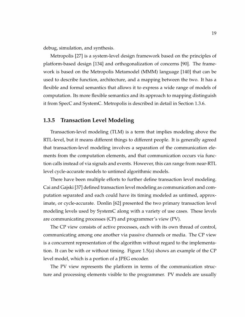
process Consumer1 that reads the values from M1. Figure 1.7 shows pieces of code
for some of the elements in this example.
Processes are active elements with each one having a single thread of execution
specified by its thread method. Figure 1.7(b) shows the sample code of process
Producer (which is instantiated in FuncNetlist as Producer1), it performs writes via
its writer port p write. The Consumer process is similar, but it performs reads via its
port p read.
Processes can only communicate through media that they are connected to via
their ports. For a port to connect to a medium it must implement compatible in-
terfaces. A port’s interface is compatible with a medium only if it is a superclass
23
interface writer extends Port {update void write(int i);eval int space();
}
interface reader extends Port {update int read();eval int n();
}(a) Interface definitions
process Producer {port writer P write;thread(){
int z=0;while(true){
P write.write(z);z) = z+1;
} // end while loop} // end thread method
} // end process P(b) Sample process code
medium M implements reader, writer{int storage;int n, space;void write(int z){
await(space>0; this.writer ; this.writer)n=1; space=0; storage=z;
}int read(){ ... }
}(c) Sample medium code
Figure 1.7: Code excerpts of elements of the example. Bolded words are the namesof particular classes, methods and variables in the code. Italics indicate specialkeywords from Metropolis.

24
of (or the same class as) an interface that the medium implements. An interface is
a set of methods implemented by a medium, which a port extending it can call.
Figure 1.7(a) shows the reader and writer interfaces for the example. The keyword
eval is used on a method to indicate that the method only ‘evaluates’ the state of
the component, but does not update the state of the component. The keyword up-
date is used on a method to indicate that the method does update the state of the
component.
Media are passive elements that implement interfaces that can be called by the
ports connected to them. This means that a medium can only be triggered by a
call from a port connected to the it. Media can have ports from which to call other
media. Since media are passive elements, the triggering of a call to a medium must
come from a process (that triggers the initial medium). Figure 1.7(c) shows some
of the code of medium M; it implements the reader and writer interfaces.
The write method in medium M makes a call to the await statement. This state-
ment is used for specifying a set of one or more atomic statements of which one is
non-deterministically selected to execute. For this case there is only one statement,
for an example of multiple atomic statements see Section 3.3.2.1. Each set of atomic
statements has a set of three semicolon-separated conditions that must be met in
order to execute. The first is a guard condition that must be true in order for the
guarded statements to be executed. The second is test-list of port interfaces that
must be available (unlocked) in order to execute, and the third is a set-list of port
interfaces that are locked (so as to be unavailable) when the atomic statements are
executed, and unlocked. In the code for medium M, the writer method’s guard
condition is the space variable being larger than 0, and its writer interface is tested
and set.
1.3.6.2 Architectural Modeling
An architectural netlist usually contains two netlists: a scheduled-netlist and a
scheduling-netlist. The scheduled-netlist is made up of processes and media and is
25
T1 Tn
CpuRtos
cpuRead
ScheduledNetlist SchedulingNetlist
Bus
Mem
busRead
memRead
Request(e,r)
setMustDo(e)
resolve()
CpuScheduler
BusScheduler
MemScheduler
GTime
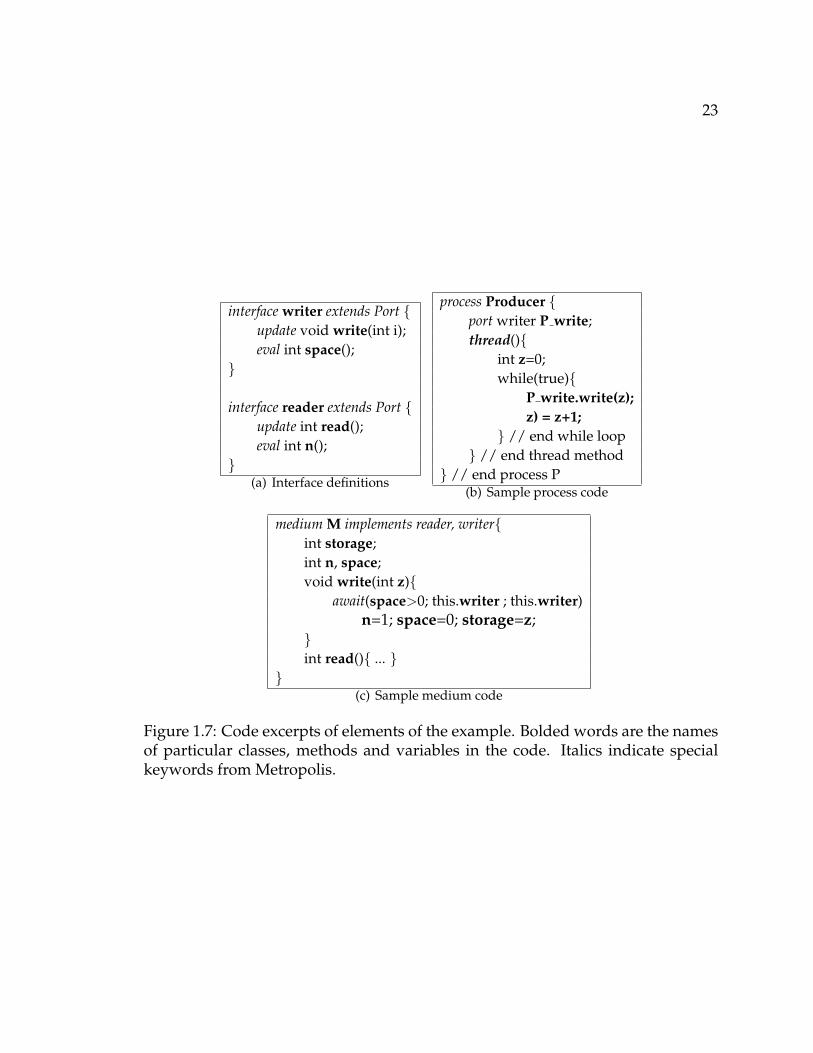
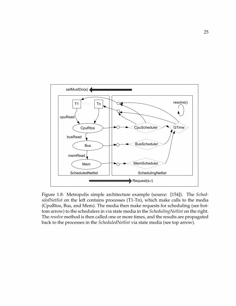
Figure 1.8: Metropolis simple architecture example (source: [154]). The Sched-uledNetlist on the left contains processes (T1-Tn), which make calls to the media(CpuRtos, Bus, and Mem). The media then make requests for scheduling (see bot-tom arrow) to the schedulers in via state media in the SchedulingNetlist on the right.The resolve method is then called one or more times, and the results are propagatedback to the processes in the ScheduledNetlist via state media (see top arrow).
26
the set of resources used to implement the architecture. The scheduling-netlist is
a netlist that manages the resources in the architecture by scheduling them and
adding costs to them; it is made up of quantity managers and state media. Figure
1.8 shows the architectural netlist from the Metropolis tutorial [154]. The netlist
on the left is the scheduled netlist and the netlist on the right is the scheduling
netlist. Media in the scheduled netlist make requests to the quantity managers in
the scheduling netlist which resolves these requests.
Quantity managers can serve two functions: scheduling and quantity annotation.
Scheduling is where multiple events request annotation and some of them may be
disabled. Quantity annotation is the association of an event with a particular anno-
tated quantity such as time or power. Because time is commonly used in system
design, Metropolis includes a quantity called GTime that represents a shared global
time.
The quantity annotation process works as follows. A process or medium makes
a request to a quantity manager, and then waits until the quantity manager grants
that request. The quantity manager resolve these requests for annotation based
on its internal policy. Communication to and from quantity managers is done via
means of specialized media called state media. The specifics of quantity managers
are detailed in Section 3.2.2.1.
Constraints and quantity managers in Metropolis operate on events. An event in
Metropolis is defined as the beginning or ending of an action. An action is a specific
process executing a labeled piece of code. The labeled code can either a component
method, or some code explicitly labeled by the user. The events for each action are
called named-events. For example, in the functional example shown in Figures 1.6
and 1.7, the beginning of process Producer1 calling the write method of M1 is an
event.

27
Bus
Arbiter
Master
CPU
Master
ASIC
Slave
Memory
SharedBus
Slave
Peripherals
Function Architecture
Mapping
Quantizer
FIFO
DCT
Huffman
FIFO
Figure 1.9: Example of combined view (CP + PV) with mapping. The two viewswere shown previously in Figure 1.5
1.3.6.3 Mapping and Constraints
Netlists can instantiate and connect all of the major components of Metropolis.
A netlist also can include constraints for temporal ordering called LTL (Linear Tem-
poral Logic) constraints [63], mapping via synchronization, and also quantitative
constraints called the Logic of Constraints (LOC) [44].
Mapping is typically done via synchronization constraints. For it, three major
netlists are instantiated: an architecture netlist, a functionality netlist, and a top
level netlist that contains the other two netlists as well as the mapping constraints.
For a one-to-one mapping the begin and end events of a method call on the func-
tion side would be synchronized with the begin and end events of a method call
on the architecture side.
Another way to look at it is that Metropolis supports both of the functional (CP)
and architectural (PV) levels of TLM concurrently and also allows them to be com-
bined through its mapping capabilities. In particular, the functional model, which

28
generally corresponds to the CP level of abstraction, is synchronized with events
in the architectural model, which most represents the PV level of abstraction. This
allows the user to use a more natural representation for the functionality and still
get accurate timing information from the architectural model. Figure 1.9 shows a
mapping that combines the CP and PV views. Section 3.3.2 has a detailed example
of mapping using Metropolis.
1.3.6.4 Execution Semantics of Metropolis
Execution begins with each process in the system executing until it hits a named
event or an await statement. Once all processes in the system have paused, then
the scheduling phase executes. In the scheduling phase quantity managers are run
and constraints in the design are resolved. Once all of the constraints are resolved
and the quantity managers are stable the processes in the scheduled netlist resume
execution. This alternation between the scheduled and scheduling netlists contin-
ues until all of the processes have exited or cannot make further progress.
1.3.6.5 Tool Framework
Figure 1.10 shows the framework for tools in Metropolis. It provides a front
end parser that reads in designs described in the Metamodel language, and con-
verts them into an Abstract Syntax Tree. Various tools are implemented by writing
a backend in Java that traverses the Abstract Syntax Tree. These tools include back-
ends for simulation [152], verification [41, 43], analysis [42], and also an interface
to the XPilot high-level synthesis tool [47]. Metropolis also has an interactive shell
where designs can be manipulated and backends can be called.

29
Meta model compiler
Verification tool
Synthesis
tool
Front end
Meta model language
Simulator
tool
...Back end1
Abstract syntax trees
Back end2Back endNBack end3
Verification
tool
Metropolisinteractive
Shell
...
Figure 1.10: Metropolis tool framework.
1.4 Levels for Modeling Embedded Software
There are a variety of levels of abstraction used to simulate software executing
on one or more target processors in an embedded system on a user’s host com-
puter. Figure 1.11 shows common levels of abstraction used for simulating soft-
ware running on a microprocessor along with their levels of detail and speed. The
term microarchitecture refers to how the implementation of the processor is repre-
sented (or if it is). Timing means the granularity of the timing, and listed speeds
are based on the best available information, which is described in the subsections
below.
RTL-level models simulate the individual signals and gates in the system, and
have the most detail and lowest performance. At the next higher level of abstrac-
tion are cycle-accurate models which simulate a program running on the target’s
microarchitecture at the cycle-level, which means that individual signals and prop-
agation delays are abstracted away. The next higher level has instruction-level

30
Register-TransferLevel Models
Cycle-AccurateModels
Instruction Level Models
Algorithmic Models
Model Speed:
Native Speed
(GHz)
~3 – ~900 MIPS
Microarchitecture / Timing:
None / None
None / Instruction
Counts
~0.1 – ~30 MIPS“Full” / Cycle-
Count Accurate
~0.1 – ~10 KHz“Full” / Signal
Level
Figure 1.11: Levels of abstraction for embedded microprocessors.
models, where only the functionality of each instruction is simulated and there is
no notion of the microarchitecture, but counts of instructions remain. At the high-
est level of abstraction are algorithmic models where the application compiled and
run on the user’s host system at native speeds; models at this level are fast, but they
have no notion of the timing, microarchitecture, or instructions of the target.
There is a significant gap between traditional methods of implementing dif-
ferent levels of abstraction and state of the art commercial tools. Furthermore,
commercial tools seldom publish meaningful measurements of their performance
and forbid their users from doing this. In order to get a good relative view of the
performance of the various tools, we divide the instructions per second (insts/sec)
performance of the host platform by the inst/sec rate of the simulator based on
numbers from a listing in Wikipedia [18]. Additionally, there are other criteria that
need to be taken into account when evaluating the performance of such measure-
ments. First, we discuss relevant work in the computer architecture world that
has had a strong influence on work in embedded systems processor simulation.
Then, we present related work on embedded systems that was used to derive the
numbers for Figure 1.11.

31
1.4.1 Computer Architecture Simulation Technologies
Many of the ideas for accelerating the simulation speed of instruction-level
and cycle-level models of microprocessors originated in the computer architec-
ture world. A common baseline for comparison is SimpleScalar [35], which is one
of the most popular microarchitectural simulators for research, and is a highly-
optimized traditional simulator. It supports several instruction sets including: Al-
pha, PowerPC, and ARM. It is listed as having a 4,000x slowdown (compared to
native execution on the host platform) for running the MIPS instruction set [6],
and our experiments with Simplescalar-ARM we found an average slowdown of
4,500x (see Figure 5.8 for details).
One key technique is that of direct execution, where an instrumented binary is
run on the host that has the same instruction-set as a target. This avoids having to
decode the instructions in software, leaving just timing and profiling information
to simulate. Shade [46] does instruction-level simulation for SPARC instruction set
processors [85] and incurs a base overhead of 3-6x compared to native execution
for basic trace collection, and it simulates a MIPS executable (on a SPARC platform)
with slowdown of 8-15x with no trace collection. FastSim [137] uses speculative
direct execution and memoization for out of order execution and is 8.5-14.7x times
faster than Simplescalar with most of the speedup coming from the memoization
(speedup without memoization is 1.1-2.1x faster).
The Wisconsin Wind Tunnel project [128] features direct execution combined
with distributed discrete event simulation on a 64-processor CM-5 from Thinking
Machines that features a slowdown of between 52x and 250x compared with the
target’s execution times. Wisconsin Windtunnel II [113] generalizes the Wind Tun-
nel work to a variety of SPARC platforms, and gives relative speedups for paral-
lel simulation2, but not absolute speed numbers. The GEMS (General Execution-
driven Multiprocessor Simulator) toolset [104] has succeeded Wind Tunnel, and
2For example, they list a speedup from 8.6x to 13.6x for simulating a 256 target system runningparallel benchmarks on a 16 host system.

32
runs by using Virtutech Simics [67] as a full-system functional simulator. This has
shown uniprocessor simulation speeds of up to 1.32× 10⁵ instructions per second
(inst/sec) [105].
Not all of the above-mentioned techniques are applicable to embedded sys-
tems, and there are different concerns for such systems. Direct execution is gener-
ally not usable for embedded systems because the host computers and the target
computers typically have different instruction sets (e.g. x86 vs. ARM). Another key
difference is that for embedded systems instruction-set simulators will often co-
simulate (simulate concurrently) with hardware at the RTL-level, which requires
having lower level interfacing (typically at the signal level). On the other hand,
embedded processors tend to be less complicated than general-purpose proces-
sors and so can often be simulated at higher speeds. The next section describes the
work in processor simulation and co-simulation for embedded systems.
1.4.2 Processor Simulation Technologies for Embedded Systems
In his seminal 1994 paper on cosimulation [132], Rowson explains different
levels for simulating software running on a target processor concurrently with
hardware in terms of their speed (in instructions per second). The ‘synchronized-
handshake’ method is equivalent to our algorithmic-level and runs at native speed,
but has no real accuracy. He lists the instruction-level models to run between 2,000-
20,000 inst/sec (instructions per second), cycle-accurate models to run at 50-1,000
inst/sec, and nano-second accurate (which is basically RTL level) running at 1-100
inst/sec. All of these are considered baseline cases, and there has been significant
work since then. To account for the improved host processors, compilation tech-
niques, and simulator optimizations we scaled these numbers up by a factor of 100
to define the low-end of the speed scale.
An important improvement to cycle-level and instruction-level models since
Rowson’s paper is compiled code simulation, where the binary decoded at compile-
time and then linked with a model of the (micro)architecture. This technique was
33
introduced by Zivojnovic and Meyr in 1996 [143] and was 100x-600x faster than
traditional interpreted cycle-accurate simulators, which they list as having speeds
between 300 and 20,000 instructions per second. When dividing the inst/sec rate
of the host platform by the inst/sec rate of their target simulator the slowdown of
compiled-cosimulation compared to native execution is roughly 34x-200x. In 2000,
Lazarescu et al. [28] developed a similar approach, but instead of doing direct
binary translation they did an assembly-to-C translation and yielded a simulator
with a speed of almost 1.3×10⁷ cycles per second on a 500 MHz Pentium III system.
Given an estimated host performance of 1.3×10⁹ IPS [18] for the host and assuming
a CPI (Cycles per Instruction) of 1 for the target processor, this is 100x slower than
native execution. VaST systems [16] sells very fast virtual processor models that
improve upon the above approaches with static analysis and also low-level hand
optimizations. In 1999 [78], Hellestrand said that their virtual-prototype models
could execute at up to 1.5× 10⁸ instructions per second on a 400 MHz host, which
is approximately 15x faster than Lazarescu’s work in the same time period and has
a slow down of only about 7x compared to native execution.
A major issue with compiled code simulators is that they cannot handle self-
modifying code, which is a key feature in most Real Time Operating Systems
(RTOSs). As a result, direct compiled code simulators have not had commercial
success. What has been successful is having high-speed interpreted simulators
that cache decoded instructions. This approach was introduced by LISAtek (now
CoWare) in 2002 [116], where they reported getting performance approaching that
of cache compiled simulators with speeds of up to 8× 10⁶ instructions per second
for instruction-accurate models generated from LISA descriptions on a 1200 MHz
Athlon. Given a host performance of 3.5 × 10⁹ inst/sec [18] for this processor the
slowdown is a factor of 440. In a whitepaper from 2005 [21] VaST gives the range
of single processor performance to be from 2 × 10⁷ to 2 × 10⁸ inst/sec for cycle-
accurate simulation; for a 2.7 × 10¹⁰ inst/sec [18] 2.93 GHz Core 2 Duo processor
this gives a slowdown of between 135x and 1350x. The speed advantages of VaST
34
are because they hand optimize their simulators and sacrifice internal visibility for
the sake of speed. Given the marketing nature of whitepapers we selected a con-
servative value of 3× 10⁷ inst/sec as the upper limit for cycle-accurate simulation
performance. Based on Rowson’s numbers, we assigned instruction-accurate mod-
els a speedup of 30x over cycle-accurate models. There are other products in this
market including offerings from Synopsys (formerly Virtio) and ARM (formerly
AXYS). Virtutech Simics [67] and the Open Virtual Platform (OVP) [48] from Im-
peras provide fast instruction accurate simulation on the order of 1× 10⁸ to 1× 10⁹
instructions per second. The OVP is free for anyone, and Simics is free for univer-
sity use.
A major consideration for embedded processor simulators is the level at which
they are interfaced with. If the model is monolithic, then it does not need to in-
terface with anything else and so has no interfacing overhead. At the transaction-
level, the interfacing occurs via function calls to shared channels. If a model is
interfacing with RTL, then it probably needs to interface at the signal level (either
directly or via an adaptor). Seamless [84], from Mentor graphics, accelerates in-
terfacing cycle-accurate instruction-set simulators (ISSs) with hardware at the RTL
level, by having a direct optimized interface to the shared memory (for commu-
nication between the hardware and software) for the ISS. It is difficult to measure
the impact of the interfacing of these different models, but the speed of simulating
hardware at these different levels serves as a good guide.
1.5 Discussion
Chapter 2 presents uniprocessor microarchitectural modeling that operates at
the cycle level and takes a trace of instructions and memory addresses from an
instruction-level simulator as input. Chapter 3 presents an approach for multipro-
cessor modeling in Metropolis at the transaction level. Chapters 4, 5, and 6 de-
scribe our timing annotation framework that operates on performance traces from

35
Cycle-Accurate
Models
Instruction Level
Models
Algorithmic
Models
Logic Gates
Layout
Actual Gates
Register Transfer
Level Models
Transaction-Level
Models
Algorithmic
Models
Annotation
Framework
Multiprocessor
Modeling
Uniprocessor
Modeling
Hardware View Software/CPU View
Timed
Instruction
Trace
Timing
Annotated
Application
Application
Code and
Binary
Figure 1.12: The work from this thesis in terms of the levels of hardware and soft-ware representation. This thesis’s work is in the green callouts and plus sign.
cycle-level models and writes the average delays to the original application source
code.
1.6 Contributions and Outline
This chapter has illustrated two main trends: the unsustainability of the low-
level implementation of the traditional design flow, and the increasing importance
of software and multiprocessing in embedded systems. It also explained key pieces
of system-level design.
This thesis concentrates on the abstraction and modeling of microprocessor per-
formance for single and multi-processor embedded systems. Figure 1.12 puts the
main pieces of work of this thesis in terms of the levels of abstraction defined for
the modeling of general hardware as well as software running on a microprocessor.
Its contributions are as follows:
• Section 1.4 in this chapter analyzed different levels of abstraction for simu-
lating embedded microprocessor performance. This sets the context for our

36
research.
• Chapter 2 presents a trace-based approach for modeling the microarchitec-
tures of processors using Kahn Process Networks that is generic, intuitive,
and highly retargetable.
• Chapter 3 describes our high level modeling of bus-based multiprocessors
by representing each piece of the system as a timed resource. This is per-
formed in Metropolis, and improves upon previous architectural modeling
in Metropolis. Also, the structure of a representative application and its map-
ping to the architecture have been performed.
• Chapters 4, 5, and 6 detail our highly retargetable timing annotation frame-
work that operates on performance traces from cycle-level models and writes
the average delays to the original application source code.After the annota-
tion the annotated code can be compiled to the native host platform and run,
with timing information, at speeds one to three orders of magnitude faster
than the cycle-accurate simulator.
From the point of view of platform-based design, this dissertation primarily fo-
cuses on the lower portion of the flow moving from the system to the architecture
platform. In particular, it concentrates on moving results from the architectural
space up to higher levels of abstraction. The uniprocessor modeling allows the
user to quickly creates platform numbers for a given instruction-set. The mul-
tiprocessor architectural model is a high level model that enables mapping, and
allows lower level results to be propagated back to it. The annotation framework
is an approach that propagates timing results gained from cycle-level simulation
up to the original source code in the form of source-level annotations.

37
Chapter 2
Single Processor Modeling
Software executing on one or more microprocessors has become a dominant
factor in the design of embedded systems. The 2004 update of the International
Technological Roadmap for Semiconductors [5] lists embedded software as one
of the key system-level design challenges, and “Design space exploration and
system-level estimation” as a key aspect of the “System Complexity” category.
Evaluating different processors and micro-architectures at the system level is diffi-
cult and thus rarely done. The first generation system-level design environments
(such as VCC [19], POLIS [26], and COSYMA [79]) provide support for at most
several ISAs (Instruction Set Architectures), and typically even fewer microarchi-
tectural instances with little or no extensibility. Second generation tools such as
Model Library [144] from CoWare and Seamless [84] from Mentor Graphics do
have better libraries of processors, but these cannot easily be extended for explo-
ration. Architecture Description Languages (ADLs) such as LISA [123] and Ex-
pression [74] are domain-specific languages for designing new processors and in-
struction sets. They can also automatically generate software tools, simulators, and
hardware from the descriptions. However, ADLs often couple the microarchitec-
ture’s description with that of the functionality, forcing the complete specification
of the processor, which can be time consuming. Microarchitectural simulators,

38
such as SimpleScalar [35], provide stand-alone environments for evaluating the
impact of different microarchitectures implementing one or more ISAs, but are
generally difficult to retarget or use at the system-level. This chapter presents a
high-level approach [107, 108] to model timing performance of a single embedded
microprocessor’s microarchitecture using Kahn Process Networks [87]. The result
is a high-level intuitive model that is retargetable, easy to extend, and fits well
within a system-level environment.
The next section presents formal definitions for modeling processor perfor-
mance. Section 2.2 describes the processor models. Section 2.3 compares the mod-
els to the ARM models from the Simplescalar [35] simulator. Then, section 2.4
reviews related work. Finally, the work is discussed and put into perspective.
2.1 Processor Modeling Definitions
A single program running on a microprocessor can be thought of as a totally
ordered trace of N instructions, where the ordering between instructions repre-
sents their logical execution order. Instruction Ii is the i-th instruction in the trace.
A microprocessor is an architectural implementation of the functionality of an in-
struction set archicture (ISA). When a program executes on a microprocessor, the
beginning and ending of the execution each instruction have times associated with
them, which transforms the instruction trace into a timed instruction trace. First,
we describe the functional aspects of the trace. Then, we describe the microarchi-
tectural aspects. Finally, we give an example and discuss how particular microar-
chitectural features can be represented in this formalism.
2.1.1 Functional Definitions
The ISA (instruction set architecture) of a processor P consists of its logical state
elements (or memories), MP , and the set of instructions that it implements IP . The

39
correct behavior of a processor running a program is the atomic sequential execu-
tion of the instructions modifying its state. All microarchitectures that implement
the ISA of P must be logically consistent with this model, even though the execu-
tion of instructions often overlap due to microarchitectural features like pipelining
and out-of-order execution.
2.1.1.1 Logical State
We call the logical state elements in an ISA memories MP refers to the set of
memories for processor P . Memories represent regular memories, condition codes,
register files, and other state elements in the ISA. Each memory mi in MP has a
unique name and can be read-only, write-only, or read-write. Each memory also has
a certain number of addressable elements n(mi), which typically is a power of 2.
The Program Counter, PC, is a special single element that stores the current lo-
cation of the program in a memory. It can be a memory itself or located in another
memory. For our purposes, we assume that every processor has a memory where
the instructions are locate, and exactly one PC that indicates the current instruc-
tion’s location in memory.
2.1.1.2 Operands
Before defining what instructions are, we first define what operands are. An
operand is a value, or a reference to a value in a memory in an instruction. OP is the
set of all legal operands for processor P . An operand has a name, which is unique
from the names of the other operands in the given instruction. A constant operand
is a value encoded directly in the instruction. It should be noted that constant
operands can only be read operands.
For a processor P , each operand o ∈ OP is characterized by the following func-
tions:
• r(o) : OP → {0, 1} is 1 if o is a read operand.

40
• w(o) : OP → {0, 1} is 1 if o is a write operand.
• M(o) : OP → MP returns the memory accessed by the operand. If M(o) =
null then the operand is a constant operand.
• A(o) returns the address indexed in the memory by this operand. It returns
null for constant operands, or for operands that have yet to have their ad-
dress calculated.
• V (o) : OP → B indicates if the value of the given operand is ready (to read
or write). This is purely used for indicating the state inside of the microar-
chitectural model. V (o) = 0 implies that o has not been read yet, if o is a read
operand, and that its value has not been calculated if o is a write operand. For
more complicated architectures additional states (e.g. ready to write/read)
may need to be added.
2.1.1.3 Instructions and Their Properties
The set of all legal instructions for processor P is IP , and it has a fixed set
of types of instructions, TP = {t1, ..., tm}, called the instruction set. Each type tx
specifies the resources used by the instruction, as well as the types of operands
used by it, but not their addresses. Each instruction works by reading operands,
performing some calculations, and then writing operands based on the result. Each
processor also a null/NOP(No Operation) instruction I∅, which has no read or
write operands and is used for microarchitectural modeling.
Each instruction Ii in the program trace has the following functions/properties
associated with it.
• e(Ii) : IP → Bn returns the vector of n-bits1 that represent the encoding of the
instruction Ii.1This assumes fixed length encoding, but this could be extended to variable length encodings.

41
• t(Ii) : IP → TP returns the type of instruction.
• n(Ii) : IP → N0+ returns the index of the instruction (e.g. n(Ii) = i) as a
non-negative integer. For I∅, n(I∅) = 0.
• R(Ii) returns the set of general read operands in the instruction. These are
defined by the instruction type, its encoding, and possibly the state of the
system.
• W (Ii) returns the set of write operands in the instruction. These are defined
by the instruction type, its encoding, and possibly the state of the system.
They access the same resources as read operands, but cannot refer to con-
stants. Each write operand updates the state of the system for future instruc-
tions.
• a(Ii) returns the address (and memory) where the given instruction is lo-
cated. We separate this from the R(Ii) because it is not dependent on the
encoding or type of the instruction. In the case of interrupts and I∅, the ad-
dress is null.
2.1.2 Architectural Definitions
This section presents definitions used for attaching performance information to
a functional execution trace of a microprocessor. First, the trace formalism is spec-
ified. Then, the refinement of the trace formalism to include stages of execution is
reviewed. Finally, the representation of different microarchitectural features using
the trace formalism is presented.
2.1.2.1 Overview of the Trace Formalism
For a given processor P , there is an application space AppTrace(P ) of legal
traces of instruction and data values, and a microarchitectural space uArch(P )

42
for modeling the timing and resources of the program executing on the proces-
sor. Time can either be defined as the set of non-negative real numbers or, for the
case of cycle-level modeling, as the set of non-negative integers.
The TimedAppTrace extends the initial trace by annotating the instruction with
begin and end times. For ax(P ) ∈ AppTrace(P ) we define :
tax(P ) = TimedAppTrace(ax(P )) = ((Ij, Begin(Ij), End(Ij)) | ∀Ij ∈ ax(P )),
and Begin(Ij), End(Ij) ∈ Time
A given application trace ax ∈ AppTrace(P ) and a given microarchitecture in-
stance uy ∈ uArch(P ), the combination yields a timed application trace as shown
below:
uy(ax) : AppTrace(P )→ TimedAppTrace(P )
The index i of each instruction Ii is a non-zero natural number indicating its
position in the trace. Given this, each instruction in any valid timed application
trace tax(P ) must have the following properties:
1. (Begin(Ii) ≤ Begin(Ij)|∀Ii, Ij ∈ ax(P ) s.t. i ≤ j)
2. (Begin(Ii) ≤ End(Ii)|∀Ii ∈ ax(P ))
2.1.2.2 Refinement to Stages
The execution of an instruction on a processor can be broken up into different
stages that comprise the full execution, such as reading operands from the register
file or writing a value to a memory. A stage is defined as a component that con-
nects to unidirectional queues via input and output ports. It reads zero or more in-
structions in as input, performs some computation, and then outputs zero or more
instructions. Each stage is a process in that it can be thought of as a program with
blocking reads from inputs and blocking writes to the outputs. A stage can access
the memory elements of the instruction set to read and/or update their state, and
43
may perform some modification of the instructions that it inputs (i.e. writing out
operand results). Dependency between stages is shown as an edge (queue) from
the earlier stage to the later stage. We call this dependency graph an Execution Flow
Graph (EFG).
Upon the execution of a trace on a model in the framework, each instruction in
the trace is assigned a time value for when it enters a stage, and another time value
when it leaves the stage. More formally, each stage Sm has two tags Begin(Sm, Ii)
and End(Sm, Ii), which respectively represent the time of the Ii entering and leav-
ing the stage. Given this ordering, we have that Begin(Sm, Ii) ≤ End(Sm, Ii). The
delay of a stage for a given instruction is calculated as the difference between the
end time and the begin time. If the stage is of constant delay, then this difference
is constant.
Another property is that for each instruction running on a microarchitecture,
the sum of the delays in its stages must be equal its total delay. Stated more for-
mally this this means that for every instruction Ii in each stage Sm in the microar-
chitecture uj :∑Sm∈uj
(End(Sm, Ii)−Begin(Sm, Ii)) = End(Ii)−Begin(Ii)
It is possible for stages and queues to have zero delay, but they cannot have
negative delay. The end tag of an instruction of one stage can be the same as the
begin tag of a successor stage that is connected to the first stage via an queue with
a zero cycle delay.
A given instruction cannot begin execution in a stage before it begins execution
in an earlier stage, although it may be possible to begin execution at the same time
as the preceding stage. An instruction can sometimes ”pass” earlier instructions,
such as in the case of out-of-order execution, but we require that the commits of
each instruction must not happen before the commits of earlier instructions (i.e.
they can happen at the same time).

44
2.1.2.3 Stages of Execution
Fetch Decode
Read
Operands Execute
Write
Operands Commit
SCSWSESRSDSF
Figure 2.1: Example of stages
Figure 2.1 shows the stages for the example laid out in this section. It is based
on the basic RISC/DLX style of microarchitecture presented in [121], and partially
inspired by the notation of the Operation State Machine [126]. While this general
style is true for all microprocessors, they can be split into multiple stages and some
of the ordering of the different stages can be in parallel or in different orders (e.g.
such as having read and decode occur in parallel such as in [121]). Below we detail
the behavior of these individual stages.
Fetch The Fetch stage, SF , loads the instruction from memory. In general, the only
operand that it depends on is the program counter PC.
Decode The Decode Stage, SD, translates the fetched instruction into a form where
its operands and instruction-type are known. The Decode stage cannot begin
on an instruction until the Fetch of it is finished.
Read This stage, called SR, gets some of the read-operand values from various
resources. Its execution may be stalled if any of its read-operands depend
on the write operand of an earlier instruction that has not yet written back
its results. It is important to note that this stage does not necessarily handle
all read operands (e.g. read operands to data memory, such as in a Load
instruction are generally handled in a later stage).
Execute Once the Read stage finishes reading the necessary operands, the Execute
stage, SE , can begin. When this stage finishes all of the instruction’s write

45
operands are given values. It may sometimes access memories, such as load
and store instructions).
Write The write stage, W , involves passing the write operand values to instruc-
tions that depend on them. This happens before the entire system state is
updated. Once it finishes, it will allow instructions that are stalled waiting
for its operand values to proceed. This stage is not strictly necessary, and
may be viewed as immediately following execute and taking no time. We
chose to separate it from execute and commit, so that the forwarding (or lack
thereof) of instruction results can be explicitly modeled.
Commit The commit stage, C, only processes an instruction when the instruction
has finished execution and all instructions before it have been committed or
will commit at the same time. It updates the state of the processor based on
the results of the instruction, making the system logically consistent.
2.1.2.4 Representing Microarchitectural Features
A wide variety of microarchitectural features can be described in terms of the
definitions provided in this section. They are specified by adding different prop-
erties and constraints to the stages and queues in the EFG, or by changing the
structure of the EFG. This is not intended to automate the design of simulators,
but it provides a context the relationships between instructions for different mi-
croarchitectural features.
Pipelining is a well known technique in computer architecture for increasing
clock speeds and allowing the execution of instructions to overlap. To enable
pipelining the execution flow of the processor is broken up into multiple stages
that have registers between them at the boundaries. Once an instruction is fin-
ished with one stage its output is passed to the registers that serve as input for the
next stage. In the next clock cycle the following instruction enters the first stage,
and the original instruction begins execution in the second stage. Since the reg-

46
isters all share the same clock, this clock can only be as fast as the slowest stage.
Also, structural and operand dependencies must be handled in order to assure
correct operation. Pipelining between execution units can be achieved by refin-
ing the queues to have a size of greater than 1. If a stage S is fully pipelined2,
then there is the restriction, for each instruction Ii that enters and leaves it, that
(Begin(Sx, Ij)−Begin(Sx, Ii)) ≥ 1 , where Ij uses stage Sx, and i < j.
Buffering is represented as storage between stages. For stages Sj and Sj+1
where the second stage has a sequential dependence on the first stage, if there is
no storage between them, then for each instruction passing between the stages we
have End(Sj, Ii) = Begin(Sj+1, Ii). Pipelining between two stages can be thought
of as having a buffer of size 1. A buffer’s size indicates the number of instructions
that can be processed by stage Sj and not consumed by its immediate successor
stage(s) before it has to stall. Unless otherwise specified a buffer operates in FIFO
order.
Branch instructions can be handled in multiple ways within this framework.
They are different from other types of instructions in that they update the PC
based on their result, and are generally processed before the execute stage of the
pipeline. One way of dealing with this having the fetch stage handle the branches
and, depending on the result of prediction, it might delay the fetch of the following
instructions. This could also be modeled at a later stage (e.g. decode).
For superscalar execution the Fetch stage SF outputs up to X instructions,
where X is the scalarity of the of the fetch unit. It can output fewer than X in
the case of branch mispredictions. We represent mispredicts as extra delay, but
do not actually fetch the extra instructions. For this to be effective, we must also
increase the number of instances of the other stages. Out of order execution is han-
dled by specifying that an instruction may enter SE before its predecessors if it is
not depending on any operands that have yet to be calculated (operand forward-
ing can be viewed in terms of when an instruction dependency is resolved (i.e. is
2By this we mean that it can accept a new instruction each clock cycle (time unit)

47
it in SW or SC).
2.2 Processor Models
This section provides an overview of the different pieces used to construct the
KPN-based microarchitectural models (these are also referred to as two process
models). Section 2.2.1 provides a high level picture of the models and their be-
havior. Section 2.2.2 explains the trace format used by the models. Then, section
2.2.3 explains how a memory system is added to the models. Finally, section 2.2.4
presents limitations of the modeling style.
2.2.1 High Level Overview
Our microarchitectural model is driven by an instruction trace generated by a
functional ISS (Instruction Set Simulator), and returns the number of cycles that
it takes to execute. To ensure accuracy the model must account for the delays of
individual instructions, the interaction between them, and the impact of limited
resources. The models described in this subsection use the channels in a cyclical
manner, where each cycle every process either reads one token from all of its in-
put channels and writes one token to each of its output channels, or, in the case
of stalling, does not read or write any channels. In order to model a particular
pipeline length, channels are pre-filled with the number of tokens equal to the
pipeline length. As long as the cyclic assumption is maintained the lengths of the
different pipelines stay constant.
This approach uses a two process model like the one pictured in Figure 2.2.
The two processes are a fetch process that handles the fetch and issue of instruc-
tions from an execution trace generated from a functional simulator of the instruc-
tion set, and an execute process that handles the execution, operand dependencies,
and forwarding delays between instructions. These models have three types of
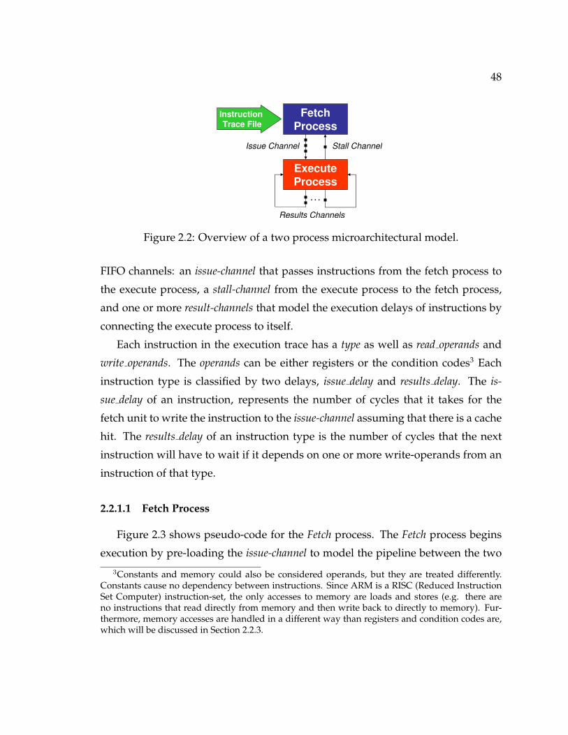
48
Fetch
Process
Execute
Process
…
Stall ChannelIssue Channel
Results Channels
Instruction
Trace File
Figure 2.2: Overview of a two process microarchitectural model.
FIFO channels: an issue-channel that passes instructions from the fetch process to
the execute process, a stall-channel from the execute process to the fetch process,
and one or more result-channels that model the execution delays of instructions by
connecting the execute process to itself.
Each instruction in the execution trace has a type as well as read operands and
write operands. The operands can be either registers or the condition codes3 Each
instruction type is classified by two delays, issue delay and results delay. The is-
sue delay of an instruction, represents the number of cycles that it takes for the
fetch unit to write the instruction to the issue-channel assuming that there is a cache
hit. The results delay of an instruction type is the number of cycles that the next
instruction will have to wait if it depends on one or more write-operands from an
instruction of that type.
2.2.1.1 Fetch Process
Figure 2.3 shows pseudo-code for the Fetch process. The Fetch process begins
execution by pre-loading the issue-channel to model the pipeline between the two
3Constants and memory could also be considered operands, but they are treated differently.Constants cause no dependency between instructions. Since ARM is a RISC (Reduced InstructionSet Computer) instruction-set, the only accesses to memory are loads and stores (e.g. there areno instructions that read directly from memory and then write back to directly to memory). Fur-thermore, memory accesses are handled in a different way than registers and condition codes are,which will be discussed in Section 2.2.3.

49
Integer issue stall = 0Boolean inst = nullpreloadIssueChannel()while inst trace.hasInstructions()
stalled = stall channel.read()if inst == null // read next instruction from the trace
inst = inst trace.readNextInst()issue stall = getIssueDelay(inst)
if stalled == false // issue instruction or bubbleif issue stall ≤ 1
issue channel.write(inst)inst = null
elseissue channel.write(bubble)
issue stall = issue stall - 1
Figure 2.3: Pseudo-code for Fetch process execution.
processes. This delay typically represents the delay of instruction fetch and de-
code. For the main execution loop, which executes every cycle, it reads from the
stall-channel, and if there is no stall then it writes either the fetched instruction
from the instruction trace or, if there is an issue stall, a bubble instruction4 with no
operands to the issue-channel.
2.2.1.2 Execute Process
Figure 2.4 shows the pseudo-code for the execution of the Execute process. Its
execution begins by pre-loading the result-channels to their configured lengths, then
the main loop is entered. In the main loop, if there is no stall from operand depen-
dencies, the next instruction is read from the issue-channel. After this the process
reads from the result-channels and updates the operand dependency table. Then
the Execute process checks to see if any of the read operands of the current instruc-
tion are unavailable and if so it sets the stall variable to true (otherwise it false).4The bubble (or empty) instructions are used to model stalls or non-operation in the microarchi-
tecture.

50
preloadResultsChannels()Boolean stalled = falseInstruction curr inst = nullwhile true
if stalled == falsecurr inst = issue channel.read()
readResultChannelsAndDoUpdate()stalled = checkOperandDependencies(curr inst)if stalled
writeResultChannels(bubble)else
writeResultChannels(curr inst)curr inst = null
stall channel.write(stalled)
Figure 2.4: Pseudo-code for Execute process execution.
If the stall variable is false, then the appropriate result channel is selected for the
instruction and it is written to it. If stall’s value is true, then no results channels are
selected, and the fetch process is informed of the stall via the stall channel. After
this, bubble instructions are written to all of the unselected result-channels, and the
value of stall is written to the stall-channel.
2.2.2 Trace Format
The microarchitectural models are driven by instruction and memory address
traces generated by a modified functional Instruction Set Simulator (ISS). Each in-
struction issued by the ISS is turned into a trace entry that consists of three ele-
ments: a string that indicates if the instruction executes (i.e. “EX”) or does not (i.e.
“NOEX”), a hexadecimal value indicating the PC (Program Counter) address of
the instruction, and the hexadecimal value of the instruction. Figure 2.5 shows the
first four entries of a trace file in the first column, and the decoded entries in the
second column.
A memory address starts with the string “MEM” and on each line is followed
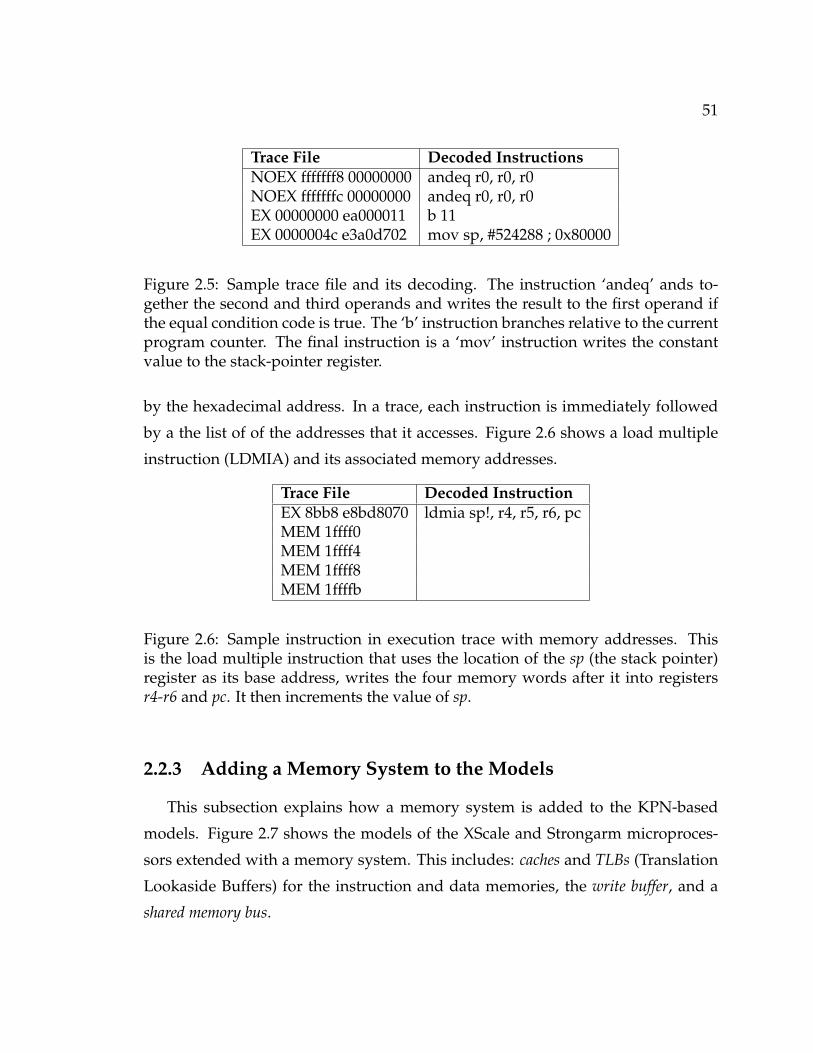
51
Trace File Decoded InstructionsNOEX fffffff8 00000000 andeq r0, r0, r0NOEX fffffffc 00000000 andeq r0, r0, r0EX 00000000 ea000011 b 11EX 0000004c e3a0d702 mov sp, #524288 ; 0x80000
Figure 2.5: Sample trace file and its decoding. The instruction ‘andeq’ ands to-gether the second and third operands and writes the result to the first operand ifthe equal condition code is true. The ‘b’ instruction branches relative to the currentprogram counter. The final instruction is a ‘mov’ instruction writes the constantvalue to the stack-pointer register.
by the hexadecimal address. In a trace, each instruction is immediately followed
by a the list of of the addresses that it accesses. Figure 2.6 shows a load multiple
instruction (LDMIA) and its associated memory addresses.
Trace File Decoded InstructionEX 8bb8 e8bd8070 ldmia sp!, r4, r5, r6, pcMEM 1ffff0MEM 1ffff4MEM 1ffff8MEM 1ffffb
Figure 2.6: Sample instruction in execution trace with memory addresses. Thisis the load multiple instruction that uses the location of the sp (the stack pointer)register as its base address, writes the four memory words after it into registersr4-r6 and pc. It then increments the value of sp.
2.2.3 Adding a Memory System to the Models
This subsection explains how a memory system is added to the KPN-based
models. Figure 2.7 shows the models of the XScale and Strongarm microproces-
sors extended with a memory system. This includes: caches and TLBs (Translation
Lookaside Buffers) for the instruction and data memories, the write buffer, and a
shared memory bus.

52
Fetch Process
Execute Process
…
InstructionTLB
SharedMemory
Bus
InstructionCache
DataTLB
DataCache
Figure 2.7: Memory model overview. TLB stands for Translation Lookaside Buffer,which is used for caching page table mappings. The write-buffer is not shown be-cause it is inside of the execute process.
2.2.3.1 Caches and TLBs
The addition of caches and TLBs is straightforward. They are implemented as
media which are checked for a hit of given address and then update their state for
a given address. The write-buffer is implemented as an array inside of the execute
process that tracks the pending store operations. The write-buffer saves the values
of pending stores and, when passed a load address, returns true if that address is
currently being stored in the memory.
For the simple microarchitectures being modeled, the instruction cache has a
simple and predictable behavior because it only reads from memory, and fetches
instructions in order. Upon a miss, in the instruction cache the issue-stall value is
increased by M , where M is the cache miss penalty. The data cache’s behavior is
more complicated because there are multiple concurrent instructions and there are
read and write dependencies between the instructions.
For a store instruction, the data cache is checked for hits on the instruction’s
53
addresses and then, if they all hit, the store instruction is moved to an S cycle delay
results channel, where S is the delay for a store instruction that hits the cache. If
any of the store instruction’s addresses miss, then they are all added to the write
buffer, and the instruction is placed in a results queue with an M cycle delay, where
M is the cache miss penalty. Upon reaching the end of the results channel, a store
instruction updates the data cache and removes its values from the write buffer.
For a load instruction, the write buffer is checked, and if it misses then the data
cache is checked. If there is a hit, then the instruction is put into a L cycle delay
results queue, where L is the results-delay for a load instruction hit. If there is
a miss, then the instruction is put into a M + L cycle-delay results queue. Upon
exiting the results queue, the load instruction updates the state of the data cache if
necessary.
2.2.3.2 Modeling a Non-Pipelined Shared Memory Bus
The memory system as described above does not model the fact that the in-
struction and data cache typically share a single bus to the memory system. This
sharing increases overall execution time because each cache must stall if it tries
to access the bus when the other has control of it. To model this, a Bus medium
which models the mutual exclusion between the two caches accessing memory at
the same time was created.
The Fetch and Execute processes each connect to the Bus medium, and call the
lock and unlock methods that it implements. When two processes attempt to lock
the bus at the same time, one of them is non-deterministically selected as the win-
ner. When the lock method is called, it returns a 1 if the lock was successful, and a
0 otherwise.
On an instruction cache miss, the Fetch process stalls its issuing until it has
successfully locked the bus. Once the instruction is issued, then it the Fetch process
unlocks the bus. On a data-cache miss, the Execute process tries to lock the bus. If
the lock attempt is unsuccessful, then the Execute process stalls until the next cycle

54
and then tries again. Once successful, the Execute process writes the instruction to
the results-channel that adds the delay of the cache miss. Upon writing back the
results from this channel, the Execute process unlocks the bus. This behavior can
be modified to model a pipelined memory bus by having both Fetch and Execute
only lock the bus for a single-cycle, instead of the whole time spent servicing the
miss.
2.2.4 Model Limitations
As implemented, the KPN-based microarchitectural models have some limita-
tions. For simplicity, the caches and translation lookaside buffers (TLBs) treat loads
and stores the same way, and only pipelined execution resources are modeled.
These could be resolved, but might impact the execution time. All of the models
discussed are single-issue models with out of order commit, which matches the
XScale and Strongarm microarchitectures. Aside from branch instructions, value-
dependent instruction latencies are not modeled because the instruction traces do
not capture the values of register operands. Finally, the instruction buffer has not
been modeled and interrupts and exceptions are treated as regular instructions.
2.3 Case Study and Results
This section compares the Kahn Process Network (KPN) models in terms of
speed and accuracy with that of the SimpleScalar-ARM models for the Strongarm
and XScale microarchitectures. The models mentioned in the chapter are using
versions of YAPI [58] written for Metropolis [27] and SystemC [8] were used. YAPI
is an implementation of Kahn Process Networks (KPN) [87] with the addition of a
non-deterministic select operator. These models developed here only use the KPN
semantics, and not the select functionality. The experiments were run on a Linux
workstation with a 3 GHz Xeon Processor and 4 GB of memory.

55
2.3.1 XScale and Strongarm Processors
The ARM (Advanced RISC Machines) [3, 102] instruction set is a 32-bit RISC
(Reduced Instruction Set Computing) developed for use in embedded systems. It
is by far the most popular instruction set for embedded applications, and is used
in a variety of applications including: cellphones, personal digital assistants such
as the Palm TX [145], and MP3 players such as the iPod [86]. The ARM instruc-
tion set is a compact instruction set that can be efficiently implemented. Over the
years there have been a number of extensions to the instruction set including: a
16-bit execution mode called Thumb, optimizations for java execution, and special
instructions for multimedia and multiprocessing.
The DEC Strongarm and Intel XScale are low-power scalar embedded proces-
sors that implement the version 4 of the ARM [102] Instruction Set Architecture
(ISA). The Strongarm [51] processor has a five stage pipeline with static branch
prediction, and has a frequency of up to 206 MHz. The XScale PXA-25x proces-
sor [45, 52] is the successor to the Strongarm, has a seven stage pipeline, dynamic
branch predication, and has a frequency of up to 400 MHz.
2.3.2 Accuracy Results
Figure 2.8 shows the accuracy of the KPN models of the StrongARM and XS-
cale microprocessors versus equivalent SimpleScalar-ARM[35, 73] configurations.
The first benchmark is a simple Fibonacci program and the last three benchmarks
are from the MiBench benchmark suite [73]. The second and third benchmarks
respectively are the small and large versions of the string-search benchmark from
MiBench. The final benchmark is the Fast Fourier Transform (FFT) from MiBench,
but reduced in size.
Table 2.1 shows the accuracy numbers of the two process Metropolis models
compared to Simplescalar. Table 2.1(a) shows the results with idealized memory
where cache and TLB misses have no cost. For the ideal case the average error

56
Table 2.1: Two process model (Metropolis) error compared with SimpleScalar withmatching configurations for real and ideal memory. Ideal memory refers to havingideal memory where every memory access is a cache hit. Real memory refers tohaving realistic delays for cache misses and bus contention. Figure 2.8 is a graphof the data from these tables.
(a) Results with ideal memory
Measurement Processor Category Fibonacci
String
Search
Small
String
Search
Large
FFT
Tiny
SimpleScalar 31,674 278,327 6,348,218 4,782,014
Metropolis 34,090 310,568 7,165,792 5,032,746Difference 2,416 32,241 817,574 250,732
Error 7.63% 11.58% 12.88% 5.24%
SimpleScalar 32,426 309,331 7,096,875 5,716,470
Metropolis 36,480 312,402 7,175,016 5,552,785
Difference 4,054 3,071 78,141 -163,685Error 12.50% 0.99% 1.10% -2.86%
Ideal Memory
Cycles
Strongarm
Xscale
(b) Results with real memory
Measurement Processor Category Fibonacci
String
Search
Small
String
Search
Large
FFT
Tiny
SimpleScalar 70,673 329,486 6,475,559 4,856,919
Metropolis 61,190 346,975 7,254,988 5,101,099Difference -9,483 17,489 779,429 244,180
Error -13.42% 5.31% 12.04% 5.03%
SimpleScalar 49,524 330,889 7,129,976 5,749,505
Metropolis 57,532 338,155 7,224,987 5,589,563
Difference 8,008 7,266 95,011 -159,942
Error 16.17% 2.20% 1.33% -2.78%
Real Memory
Cycles
Strongarm
Xscale
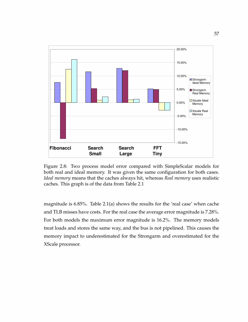
57
-15.00%
-10.00%
-5.00%
0.00%
5.00%
10.00%
15.00%
20.00%
Fibonacci Search Search FFT
Small Large Tiny
StrongarmIdeal Memory
StrongarmReal Memory
Xscale IdealMemory
Xscale RealMemory
Figure 2.8: Two process model error compared with SimpleScalar models forboth real and ideal memory. It was given the same configuration for both cases.Ideal memory means that the caches always hit, whereas Real memory uses realisticcaches. This graph is of the data from Table 2.1
magnitude is 6.85%. Table 2.1(a) shows the results for the ‘real case’ when cache
and TLB misses have costs. For the real case the average error magnitude is 7.28%.
For both models the maximum error magnitude is 16.2%. The memory models
treat loads and stores the same way, and the bus is not pipelined. This causes the
memory impact to underestimated for the Strongarm and overestimated for the
XScale processor.

58
Table 2.2: Simulation performance measurements in cycles/second.
Mode Processor
Base
Metropolis
Optimized
Metropolis
Optimized
SystemC
Simplescalar
ARM
Strongarm 2,000 5,800 66,000 920,000
Xscale 2,000 6,100 67,000 1,010,000
Strongarm 1,500 5,900 60,000 810,000
Xscale 1,500 6,000 60,000 890,000
Ideal
Memory
Real
Memory
2.3.3 Performance Results and Optimizations
Table 2.2 shows the performance of different versions of our models executing
the search-large benchmark from MiBench [73]. The first column shows the base
Metropolis models without performance optimizations. The second column shows
the results of optimized Metropolis models, and the third column shows the execu-
tion times of the optimized model ported to SystemC. The unoptimized Metropolis
models performed at roughly 2,000 cycles/second, which is clearly unacceptable.
Examining profiling results revealed several reasons for the slow simulation rate.
By applying the below described optimizations performance was increased by a
factor of thirty.
The first optimization was to switch the result-channels from general FIFO chan-
nels to fixed size internal arrays. Given the cyclic execution of accessing the FIFO
channels, they stay the same length and so there is no need to do bounds check-
ing or resizing on them. Furthermore, since the Metropolis simulator’s scheduler
uses a media-centric scheduling approach, and by changing these media to fixed
arrays the greatly reduces the scheduling overhead. This optimization increased
performance by approximately a factor of three.
The second optimization was porting the models from Metropolis to SystemC
[8]. SystemC is a less general framework than Metropolis that directly implements
discrete event simulation in its kernel (as opposed to using the Global Time quan-
tity manager), and does not have the support for non-determinism, mapping, or
quantity annotation. Thus, SystemC typically has better simulation performance

59
than Metropolis5. Given this and the fact that Kahn Process Networks are easily
modeled in SystemC, it made sense to switch to it. This modification was achieved
by modifying the SystemC code generated by the Metropolis SystemC based sim-
ulator to run in plain SystemC using bounded FIFO channels. Because the FI-
FOs were of bounded size, it was necessary to use blocking writes to avoid dead-
lock. Porting to SystemC gave a further performance increase of approximately
ten times when compared to the optimized Metropolis version. While these per-
formance increases are encouraging they still are not as fast as Simplescalar, which
ranged from 800 KHz to 1 MHz on the host system. This leaves a gap of roughly
15x between the SystemC KPN-based models and Simplescalar. There are still
many inefficiencies and potential optimizations present, which will be discussed
next.
2.3.3.1 Theoretical Performance Analysis
This section analyzes the theoretical performance limits of the KPN-based mi-
croarchitectural models. This analysis calculates the Worst Case Execution Time
(WCET) for simulating a single cycle in the microarchitecture by assuming that
an instruction is fetched and decoded each cycle to put a bound on the simulator’s
speed. All of this analysis is based upon the below variable definitions:
• R - The number of Results-Channels used by the model. Specifically this is
equal to the number of different delays used in the execution units.
• TF - Time to fetch an instruction (i.e. read an instruction word from the trace
file). For models with memory this includes accesses to the instruction cache
and instruction TLB.
• TD - The time to decode an instruction word.5In [152], Yang et. al, showed that this overhead can be mitigated in some cases through opti-
mization of the generated simulator, but the two process models in this chapter are tightly coupledand benefit little from his optimizations.

60
• TI - The time to issue an instruction to a results channel. For models with
memory this will include accesses to the data cache and data TLB for loads,
stores, and other instructions that access memory.
• TFR - The time to read from a FIFO channel.
• TFW - The time to write to a FIFO channel.
• TAR - The time to read from an array channel.
• TAW - The time to write to an array channel.
• TRU - The time it takes for the execute process to update its operand state
based on reading the results from a single a results channel.
The distinction between FIFO channels and array channels is that FIFO chan-
nels are communication media that do boundary checks and can be resized, whereas
each array channel is made from an arrays of a fixed length where reads and writes
alternate (i.e. the cyclic assumption). The array channels have significantly better
performance because they don’t do the boundary checks and, since they are just
regular variables, they don’t cause a context switch between processes like com-
munication media does.
For the initial unoptimized implementation the Worst Case Execution Time
(WCET) for simulating a single cycle is specified as:
WCETBase = TF + TD + TI + (R + 2) ∗ (TFR + TFW ) + R ∗ TRU
In this case a new instruction is fetched and decoded, and all of the channels
are read from and written to. This includes the result-channels as well as the issue-
channel and the stall-channel. Finally, all of the operand dependencies are updated
from each result channel.
Below specifies the formula for the optimized Worst Case Execution Time for
simulating a single cycle, WCETOpt, where each result-channel becomes an array
channel. Thus, it is specified as:

61
WCETOpt = TF + TD + TI + 2 ∗ (TFR + TFW ) + R ∗ (TAR + TAW ) + R ∗ TRU
This means that there are two FIFO reads and writes each cycle instead of R +
2, which reduces the number of potential context switches and also the overall
execution time.
Other optimizations can be viewed in terms of these formulas as well. Caching
decoded instructions or pre-decoding traces can reduce the impact of TD. Simu-
lating the microarchitectural models concurrently with a functional simulator re-
duces the overhead of TF , since it becomes either a shared variable or interprocess
communication, both of which are faster than file input.
2.4 Related Work
SimpleScalar [35] is one of the most popular microarchitectural simulators for
research. It supports several instruction sets including: Alpha, PowerPC, and
ARM. Because of the emphasis on optimization, it is programmed using very low
level C-code with many macros, making it difficult to modify or retarget. While
it does support a wide range of parameters for configuring the memory system
and branch predictors, it assumes a fixed length pipeline and requires assigning
each instruction to a fixed delay resource. These restrictions make it difficult to
faithfully model a real microarchitecture and its fine-grained instruction delays.
Our models are at a higher level of abstraction, allow for more detailed instruction
delays, and are easier to modify and reuse. For example, Simplescalar issues load
and store multiple instructions in a single cycle, whereas both the Strongarm and
XScale implement them with microcode and so take a variable number of cycles to
issue them.
In [82] Hoe and Arvind use term rewriting systems to describe hardware in
terms of state elements and then logical rules based on these elements. The state
elements include: registers, FIFOs and arrays. Then rules based on the state for
62
transforming the system are specified, and control logic for the described system is
synthesized. As an example they synthesize a simple 5-stage-pipelined processor
with area and speed comparable to that of a hand-coded implementation. More
recently, Hoe and Wunderlich [151] prototyped an Itanium microarchitecture on
an FPGA using the Bluespec language, which also uses term rewriting systems.
Our work is just aiming at doing modeling of performance, so it uses a simpler
specification based on two sequential programs.
The Liberty Simulation Environment [141] provides a highly composable envi-
ronment for constructing cycle-accurate simulators, at a medium grain of detail.
It uses the Heterogenous Synchronous Reactive model of computation [65] and a
flexible handshaking protocol, which makes it quite composable, but reduces per-
formance. In [124], Penry et al. perform significant optimizations, but even the
hand customized results perform at 155 KHz, which is roughly 25% of the speed
of Simplescalar’s out of order model running on a similar machine.
The Operation State Machine (OSM)[126, 125] is a formal framework for mod-
eling embedded microprocessors and generating fast simulators. It separates the
modeling of the operation of instructions and the hardware resources present in
the microarchitecture. The operation of a single instruction is represented as a fi-
nite state machine, called the Operation State Machine. Transitions between states
often require requests to the hardware side to token managers for obtaining, query-
ing, and releasing tokens. Each token manager represents a resource: such as a
pipeline stage, a register file, or an execution unit. Each instruction in the system
has its own OSM with its own state, and the interaction of the different OSMs is
modeled via token managers. The hardware side uses the Discrete Event MOC,
and the operation side operates synchronously on each clock cycle. It achieves
a performance of roughly 1 MHz and is simplifies complexity. Our work is at a
coarser level of granularity, and also features the separation between timing and
functionality.
In [129], Reshadi and Dutt used a modified Petri-net description called Re-
63
duced Colored Petri Nets to formally describe and synthesize very high perfor-
mance simulators of up to 10 MHz. Our work is at a coarser level of granularity
than the above-mentioned environment. Given the cyclic nature and behavior of
the KPN-based models it is possible to statically schedule them, which should im-
prove performance further. To have a achieve comparable performance the KPN-
based models would need to be recoded from scratch in highly optimized low level
C or C++ code, and implement many of the optimizations previously mentioned.
2.5 Discussion
This chapter presented an intuitive and generic high-level model of microarchi-
tectural performance written in Kahn Process Networks using two concurrent pro-
cesses communicating via FIFOs and also a shared memory bus. This model is very
portable because it separates the microarchitecture modeling from the functional
modeling, and it does not need to implement the instructions, only decode them. It
can quickly be configured to explore a variety microarchitectures by changing the
lengths of the channels, the configuration of the memory system, and the code that
determines which results channel that an instruction is issued to. This is in con-
trast to traditional simulators that are written sequentially and have to perform
non-intuitive tricks like simulating the pipeline backwards. Other related work
was generally at a lower level of abstraction than ours as well.
In experiments our models achieved good accuracy, and their initially poor per-
formance were improved by a factor of over 30. There remain more opportunities
to improve performance. The performance was broken down analytically, and the
potential optimizations were explained in terms of this analysis.

64
Chapter 3
Multiprocessor Modeling
Embedded system design requirements are pushed by the often conflicting con-
cerns of increasing algorithmic complexity, low-power requirements, decreasing
development window times, and cost pressures for design and production. Fur-
thermore, in many domains, such as cellular phones and set top boxes, flexibility
and upgradeability are key concerns because of evolving standards and the use
of software for product differentiation. This has pushed wireless chip vendors
to develop specialized multiprocessors for implementing Software Defined Radio
(SDR). These systems are a good design point in terms of power, performance,
and flexibility. However, because of their concurrency and specialization they can
be difficult to program so that they meet performance requirements Furthermore,
evaluating the performance of different application mappings on them typically
involves the use of slow cycle-level simulators, expensive prototypes, or high-level
models. This chapter develops a high level model of a multiprocessor architecture,
a high level model of a representative application, and associates them together
with a high level mapping of the functionality onto the architecture.
A key challenge of high-level modeling is to keep the models abstract enough
to be fast, small, and flexible, but to have enough detail to achieve good accu-
racy. This must be true from the point of view of the architecture, the functionality,
65
and the mapping of the functionality onto the architecture. However, the majority
of modeling styles represent the model in terms of either the functionality or the
architecture. Functionally-centric models are often untimed or highly inaccurate
because they do not take into account the architecture of the model. Architecture-
centric models force the modeler to specify the functionality as a direct mapping
to the architecture, which reduces its flexibility and makes it harder to explore
different implementations. The Metropolis system-level design framework allows
a natural function-centric description of the functionality to be mapped on to an
abstract model of the architecture. This allows for the benefits of both function-
centric and architecture-centric design styles.
This chapter describes using Metropolis to create a high-level model of the ar-
chitecture of a bus-based multiprocessor and then perform high-level mapping of
a representative application to it. This approach models the system’s communi-
cation structure in detail and abstracts the computation elements by representing
them as simple timed resources. It leverages the concepts of orthogonalization of
concerns [90] and platform-based design [134] to create a generic and highly reusable
model. Its improvements upon the previous research are:
1. The significant simplification of the components and interfaces used.
2. Completely moving scheduling of architectural resources into the domain of
quantity managers.
3. The application of an access pattern that allows for intuitive and reproducible
results using quantity managers for scheduling and annotation.
This is demonstrated with the modeling of the MuSIC Software Defined Radio
(SDR) architecture from Infineon and the mapping of the data flow of the payload
processing portion of the receive part of the 802.11b wireless local-area networking
standard [1] to it. The functionality is represented in a way that is not biased to-
wards the architecture and that eases reuse. The mapping assigns pieces of compu-

66
tation in the functionality to computational resources in the architecture, allowing
cost from the architecture to be attached to the functionality.
The next section reviews software defined radio, the MuSIC architecture, and
previous work in architecture modeling using Metropolis. After this, the simpli-
fied architectural model is presented. Then, the functional application model and
the mapping of it to the architecture are explained. Section 3.4 presents results of
the model. Finally, the chapter is summarized and discussed.
3.1 Introduction
3.1.1 Software Defined Radio
Software Defined Radio (SDR) [10, 36, 133] is where the majority of the sig-
nal processing for a wireless system is done digitally. It is considered especially
promising for next generation cellular networks; Sadiku and Akujuobi [133] de-
scribed it as “...the technology of choice in several wireless applications such as
GSM and AMPS.” The potential advantages to this approach including: greater
flexibility, lower costs, faster time to market, and longer product lifetimes. With an
SDR platform it is possible to upgrade to newer standards via firmware upgrades
and even to adjust in real time to changing network conditions. The disadvantages
of this approach are increased power consumption and reduced performance com-
pared to direct hardware implementations.
Despite its promise, SDR is still a piece of ongoing work. Sadiku and Aku-
juobi [133] stated that “Since the computational load of SDR is on the order of
billions of operations per second, it is extremely challenging to implement a SDR
in a battery-powered terminal.” Signal processing applications tend to have high
data-level parallelism and so one effective approach is to use a multiprocessor sys-
tem clocked at lower speeds. Much industrial and academic research has gone on
into developing such architectures, below we overview the project used to drive

67
our modeling and annotation work.
3.1.2 the MuSIC Multiprocessor for Software Defined Radio
Multi-Layer Bus
Finite Impulse Response (FIR)Filter
Bank 1
Bank 2
Bank 3
Bank 4
Turbo ViterbiDecoder
External Memory Interface (Flash/DRAM)
Peripherals
Shared Memory
(RF) Radio FrequencyInterfaces
SIMD Core 1
SIMD Core 2
SIMD Core 3
SIMD Core 4 Bus
Bridge
Control Processor
Local Mem.
Local Mem.
Local Mem.
Local Mem.
I & D Cache
SIMD Core Controller
PE1 PE2 PE3 PE4
I & DCache
SIMD Core Cluster
Multi-Tasked SIMD Core
Digital Baseband Processing
Local Memories
Processing Element (PE) Array
Figure 3.1: MuSIC Architecture for software defined radio (SDR)
MuSIC (Multiple SIMD Cores) [31, 127] is a heterogeneous multiprocessor for
software defined radio (SDR) designed by Infineon. It features high-performance
digital signal processing capabilities and is programmable for a large level of flex-
ibility. Target application areas include cell phones, wireless networking, and dig-
ital video. Figure 3.1 shows the MuSIC system architecture.
The bulk of the architecture’s processing power lies in a cluster of four multi-
tasked SIMD cores. Each SIMD core, pictured at the top of the figure, features four

68
processing elements (PEs) specialized for signal processing each with its own local
memory, and a RISC control processor for each context. The control processors run
a custom multiprocessor RTOS called ILTOS [136], and each one can run a single
thread. MuSIC also features an ARM processor for control layer processing, and
domain specific accelerators for FIR (Finite Impulse Response) filtering and Turbo-
Viterbi decoding.
The baseband signals enter and exit the system via the RF (Radio Frequency)
interfaces. Data can reside at three number main levels. Each SIMD core has its
own local memory that it uses to perform its computation on. Also, there are four
banks of shared memory that are accessed via a multi-layer bus. Finally, exter-
nal memory and peripherals can also be accessed over a separate communication
system, which the SIMD clusters can access through the bus bridge.
3.1.3 Prior Architectural Models in Metropolis
Figure 3.2 shows the basic structure of the simple architecture example in the
Metropolis distribution [154]. The netlist shown contains two other netlists: the a
scheduled-netlist and a scheduling-netlist. The scheduled-netlist consists of media rep-
resenting architectural elements for communication and computation–in this case
a CPU with an RTOS (called CpuRTOS), a Bus, and a Memory–and processes that
make calls to the CPU. The scheduling-netlist has a quantity manager for scheduling
each architectural element which then connects to the global time quantity man-
ager (called GTime). All of these connections are done via state media. While
only individual architectural elements are shown in the figure, the simple archi-
tecture example actually features a multiprocessor system with multiple busses
and shared memories. In it the top level netlist is configured to connect each
CPUs to any or all of the buses, and each bus to any or all of the shared memo-
ries by being passed two-dimensional boolean arrays that indicate the connectiv-
ity. The simple architecture performs timing annotation and scheduling decisions
by chaining quantity managers and their requests together, which can be hard to

69
T1 Tn
CpuRtos
cpuRead
ScheduledNetlist SchedulingNetlist
Bus
Mem
busRead
memRead
Request(e,r)
setMustDo(e)
resolve()
CpuScheduler
BusScheduler
MemScheduler
GTime
Figure 3.2: Metropolis simple architecture example (source: [154]). The Sched-uledNetlist on the left contains processes (T1-Tn), which make calls to the media(CpuRtos, Bus, and Mem). The media then make requests for scheduling (see bot-tom arrow) to the schedulers in via state media in the SchedulingNetlist on the right.The resolve method is then called one or more times, and the results are propagatedback to the processes in the ScheduledNetlist via state media (see top arrow).

70
debug because it concurrently mixes scheduling and annotation. The simple ar-
chitecture example also features time-based arbiters for FIFO (First In First Out)
and Time-Sliced scheduling of shared resources. This is quite similar to the work
presented in this chapter, but it has a few key differences. Our work is very sim-
ilar, but is more specialized in the connection patterns. Our work also adds: bus
bridges, specialized accelerators, and features quantity managers for implement-
ing Fixed-Priority and Round-Robin scheduling. This chapter’s work separates the
use of quantity managers into two steps: first the scheduling is performed, and
then timing annotation occurs. Furthermore, our work features memory-mapped
I/O (input/output), whereas the simple architecture directly references the differ-
ent slaves which is less natural.
In [59, 60], Densmore et al. develop and use a high level model the Xilinx Vir-
texII Pro FPGA (Field Programmable Gate Array) [55] in Metropolis. This model
is quite similar to the simple architecture example, but it focuses on the features of
the FPGA and connects to a performance characterizer of the FPGA’s communica-
tion system. In particular, it models point to point communication via FSL (Fast
Simplex Links) [54] unidirectional channels. A subset of these models consisting
of multiple MicroBlaze soft-core processors [53] communicating via FSL links and
each accessing its own local memory on the FPGA have been used to model the
performance for mapping exploration of the Motion-JPEG [56] application and a
portion of the H.264 video compression standard [88]. The model features Fixed-
Priority and FIFO arbitration that are implemented in the same manner that the
simple architecture does. In general this model is somewhat lower level and more
specialized than the work described in this chapter. The FSL interfaces are simple
reads and writes like those used by our models, but the bus reads and writes, are
broken into multiple transaction events1.
There have also been some lower-level modeling done using Metropolis. In
1These involve requests, transfers, and acknowledges for the addresses and then requests andacknowledges for the data. With this multiple protocols can be described.

71
[20], Davare et al. model the Intel MXP5800 image processor and the mapping
of a JPEG encoder to it in Metropolis. Like our work, they also separate the re-
quests for scheduling from requests for annotation. They use processes and me-
dia for the arbiter structure on the bus. In [153], Zeng et al. present a model for
a CAN(Controller Area Network)-based architecture used for automotive applica-
tions, and a mapping of a supervisory control application to it. It features preeemp-
tive fixed-priority scheduling at the CPU level, and non-preemptive fixed-priority
scheduling of the CAN bus. It contains many of the low level details of the CAN
architecture and features a refined processing element. Both of these pieces of work
are quite specialized and are at a lower level than the work in this chapter. The im-
age processor work models a network of processors inside of one of 8 processing
elements, which is equivalent to us modeling the internal structure of the SIMD
processor instead of representing it as a single resource. The automotive model-
ing represents the processing elements as a netlist of resources, whereas we treat a
processing element as a single resource.
In [40], Chen models MuSIC in Metropolis at a level similar to that of the sim-
ple architecture example. It also models a set of processors communicating with
shared memories via multiple buses. It does have several key differences:
1. It specializes the different processing, communication, and memory elements
and it features a fixed bus topology, which makes it less flexible but simpler
to configure (i.e. it is configured by passing the number of SIMD processing
elements used, and does not require connectivity arrays). Our work offers
similar levels of configurability.
2. It features memory mapped I/O that translates bus reads and writes at a
given address into the appropriate reads and writes at a bus slave– this is im-
portant because it allows the models to be driven by address traces generated
from lower level models. We also use memory mapped I/O.
3. It performs bus scheduling by using a special BusArbiter process. Our models

72
eliminate the bus arbiter process and add quantity managers scheduling of
the bus, bus-masters, and bus slaves.
4. It supports a lower level protocol for accessing the bus than does the simple
architecture, and has specific methods for checking the bus status and locking
and unlocking it. We found this level to be error-prone, overly complicated,
and unnecessary for our purposes of high-level mapping. Because of this,
we switched to a level similar to that of the simple architecture that features
blocking read and write methods.
The work presented in this chapter is an extension of Chen’s models. It improves
on them in the following ways: it is more generically and succinctly specified, it
provides scheduling in a more orthogonal manner by using quantity managers,
and, as a result of the first two improvements, it significantly reduces the number
of interface methods used. The next section overviews the extended models and
highlights the improvements.
3.2 Architectural Modeling
This section describes the high-level modeling of a bus-based multiprocessor.
Section 3.2.1 explains the models of the computation and coordination architec-
tural elements in the system. Section 3.2.2 details how scheduling and timing an-
notation are specified. Section 3.2.3 explains the specifics of the models used for
MuSIC.
3.2.1 Modeling Computation and Communication
Like the work from Chen [40], the major components of the architecture are
broken up into Buses, Bus-Slaves, and Bus-Masters. However, since this work puts
the scheduling into the domain of quantity managers and employs significant code

73
reuse the number of interface methods used are significantly reduced (20 vs. over
100) and the coordination behavior is far more decoupled than in Chen’s models.
Bus 1
Master0
P1_0[0] … P1_0[N]
Bus 1
Bus
Slave
Bus
Scheduler
Bus Slave
Scheduler
Bus
Bridge
Bus 2
MasterBus 2Bus Master
Scheduler
P2[0] … P2[N]
process
medium
quantity
manager
KEY:
Bus 0
Bus 0
Master0
P0[0]
Figure 3.3: Simplified view of the high-level architecture model. Arrows indi-cate the direction of the API method calls. The scheduling quantity managersfor Bus1Master0, Bus1, and BusSlave are shown. For clarity the other schedulingquantity managers, the state media, and the global time quantity manager are notshown.
Figure 3.3 shows a simple example with three buses, three bus masters, a bus
bridge, and a single bus slave. Aside from the bus bridge, all other media do have
connections to schedulers and global time. Also, state media and global time are
not pictured; They will be explained in Section 3.2.2.
Figure 3.4 shows the read and write interface methods used by Bus-Masters,
Bus-Slaves, and Buses in the models. Figure 3.4(b) shows the interface methods
used by the buses and the bus slaves. All of the methods have master id as their
first argument, which indicates where the function call came from and is used to
do scheduling. The read method takes in an address and returns the data present
at that location as an integer. The multi read method is similar but it also takes in a
size argument and returns an array of integers. The write and multi write methods

74
// Read and Multi-read Methodsupdate int read(int bus type, int addr);eval int[] multi read(int bus type, int addr, int size);
// Write and Multi-write Methodsupdate void write(int bus type, int addr, int data);update void multi write(int bus type, int addr, int[] data, int size);
(a) Interface methods for bus-masters.
// Read and Multi-read Methodsupdate int read(int master id, int addr);eval int[] multi read(int master id, int addr, int size);
// Write and Multi-write Methodsupdate void write(int master id, int addr, int data);update void multi write(int master id, int addr, int[] data, int size);
(b) Interface methods for buses and bus-slaves.
Figure 3.4: Interface methods used for buses, bus-slaves, and bus-masters. Theupdate keyword indicates that the interface method updates the state of the me-dia that implements it. The eval keyword indicates that the media’s state is notchanged by a call to the method.
have a similar structure as their read counterparts, but they return nothing and
they write to bus-slaves at the appropriate addresses. Figure 3.4(a) lists the read
and write interfaces used by bus masters. They are almost identical to those used
by buses and bus-slaves, except the first argument is now the bus type that is being
written to. This is to deal with the fact that different buses may be used to access
the same address space.
It must be noted that all of these interfaces are blocking, which means that they
stall until they can execute successfully (e.g. a resource is available). Chen’s mod-
els provide API functions for locking and unlocking resources as well as support-
ing unsuccessful (i.e. non-blocking) reads and writes. This is something that can
be useful for low-level programming, but is needlessly complicated for high-level
functional applications that use APIs that ensure that reads and writes are always
successful, which is the case for this work.
75
3.2.1.1 Bus Masters
Bus-Masters are media that implement the BusMasterInterface interface and ac-
cess one or more buses. They use quantity managers for resource scheduling and
timing annotation. All masters provide read and write methods for accessing the
buses that they are connected to, and these methods are shown in Figure 3.4(a).
With the exception of BusBridge all of the masters also have execute methods for
modeling processing time, and are passed cycles. Each master is parameterized
with a cycle-time used for execution as well as a unique master-id number for
each bus that it is a master of. Each master has its interface methods called by Bus
Master Processes, which are further explained in Section 3.3.2.1.
3.2.1.2 Buses
All buses in the system implement BusInterface and are derived from the Base-
Bus medium. Each bus instance is called by the bus-masters connected to it and
then in turn accesses its bus-slaves through its ports. BusInterface is shown in Figure
3.4(b) and has four API-methods: read, write, multi read, and multi write.
Buses are specialized through their parameters and also by implementing the
decode and shiftAddress methods. The decode method takes in an address as an argu-
ment and selects the appropriate bus-slave. The shiftAddress method also takes in
an address and calculates the appropriate offset given the address mapping of the
slaves. There are a number of parameters for configuring the buses. CLK FREQ
is the bus’s clock frequency in MHz. NUM MASTERS is the number of masters
using the bus, and NUM SLAVES specifies the number of slaves being used by the
bus. NUM READ CYCLES and NUM WRITE CYCLES respectively indicate the
number of cycles used to read and write an element via the bus. BaseBus also has
parameters that indicate its master ID number for the shared memories and RF
(Radio Frequency) interfaces.

76
3.2.1.3 Bus-Slaves
Bus-slaves are media that are typically accessed via the bus using read and
write methods. The only bus-slave in this model is SharedMem, which represents
a shared memory element2. Each has a STORAGE SIZE parameter indicating the
number of elements stored in it, a parameter called CLK FREQ that indicates clock
frequency of the bus slave in MHz, and cycle counts for individual reads and
writes.
3.2.1.4 Bus Bridges
A Bus-Bridge provides access for the masters of one bus to the slaves of another
bus. It does this by serving as a slave for the first bus, and a master of the second
bus. Like buses and bus slaves it is also configured with a frequency as well as
cycle counts for accessing it. In Figure 3.3 the bus bridge, BusBridge, is a slave of
Bus2 and is a master of Bus1.
3.2.2 Modeling Cost and Scheduling
The models as so far presented offer behavior, but have no notion of timing
and their only notion of resource scheduling is having mutual exclusion, where
only one process at a time can enter critical sections of code, and non-deterministic
scheduling of resources. This section explains how quantity managers are used to
model both timing annotation and resource scheduling. Time is modeled by us-
ing a built in quantity manager called GlobalTime, so these annotations will not be
explained in detail. The following three pieces will be presented: where quantity
managers and state media are used in the models; the use of quantity managers
for scheduling; and a usage pattern for integrating annotations with scheduling.
2The Bus-bridge is also a bus-slave, but since it is also a master it is discussed in a separate section.

77
Global
Time
Bus 1
Master0
P1_0[0] … P1_0[N]
Bus 1
Bus
Slave
Bus
Scheduler
Bus Slave
Scheduler
Bus Master
Scheduler
Bus 0
Bus 0
Master0
P0[0]
Process
Medium
Quantity
Manager
KEY:
Regular
Connection
State
Media
Connection
Figure 3.5: Simplified view of a high-level architecture model with state mediaand quantity managers. State media are the small unlabeled circles. Arrows indi-cate the direction of the API method calls for connections to regular media. Con-nections via state media are shown by the undirected lines. For readability, thefollowing items are omitted: the connections from Global-Time to the state mediaof the processes, and the schedulers for Bus0Master0 and Bus0.
3.2.2.1 Netlist Structure with Quantity Managers and State Media
Figure 3.5 shows the basic netlist structure for a system with two bus masters,
two buses, and a single bus slave. It also shows the state-media, quantity man-
agers, and their connections. Since the Bus0 and Bus0Master0 are connected to
only one process, so there is no need for scheduling; Despite this they are still con-
nected schedulers, but this is not shown in the figure. Bus1, Bus1Master0, and the
bus slave all potentially have contention and so their connections to schedulers are
shown.
There are two points required for connecting quantity managers. First, a con-
nection via state-media from the requester of the annotation (or scheduling) must

78
be made; which in this case this is from the different resources to the quantity
managers. Second, a quantity manager must connect via state-media to each of
the processes that may request it.
3.2.2.2 Scheduling using Quantity Managers
This work implements the Round Robin and Fixed Priority scheduling policies
using quantity managers. These are both extensions of the SingleResourceArbiter
base quantity manager and can be used interchangeably. The main methods im-
plemented by quantity managers are: request, resolve, stable, and postcond.
request is a method used to make annotation requests. It is passed an event to an-
notate, as well as an object of the type RequestClass, which can be extended to
contain more information for scheduling. For the scheduling policies imple-
mented in this work, RequestClass is extended into SchedReqClass that takes
the boolean argument unlock, which indicates if it is an unlock or lock re-
quest, and the integer argument master id that specifies the ID number of the
master requesting the resource.
resolve is a method used to perform the actual scheduling based on a list of re-
quests to the quantity manager. Based on this it enables and disables the
different events via state media connected to the events’ processes. For fixed-
priority arbitration, the largest (or smallest) master ID numbers are favored.
For round-robin arbitration, the quantity manager contains a variable that
indicates the favored master.
stable is a method used for iterative scheduling. It returns ‘true’ once the schedul-
ing is finished. Typically, the resolve method keeps getting called until the
stable method it returns true. The fixed-priority and round-robin schedulers
both resolve in a single step, so their stable methods always return true. This
is not true for other schedulers which may have iterative resolution.

79
postcond is the method called after scheduling is finished and the stable method
returns ‘true’. It updates the favored master ID number for round-robin
scheduling, and does nothing for fixed-priority scheduling.
3.2.2.3 Usage Pattern for Quantity Managers
This subsection details a protocol for using quantity managers for both timing
annotation and scheduling of shared resources for the bus, bus-slave, bus-master
components. It has been demonstrated to work at all three levels of resources
in the architecture, and shown to be robust. The main idea is to separate the
scheduling requests from the annotation requests, and to perform the scheduling
requests first. Doing it this way ensures that there are no unintended interactions
between the scheduling and annotation, which both can be iterative and quite com-
plicated. The simple architecture example from the Metropolis distribution [154]
makes scheduling requests from the annotation quantity manager, and thus can
suffer interactions between the two.
Figure 3.6 shows pseudo-code for doing the scheduling and then timing anno-
tation for the shared-memory medium. The top box has the annotation portion of
the read method, which requests a lock of the medium, calls the timed read method,
and then unlocks the medium. The timed read method, in the lower box, reads the
addressed value from memory, requests a given delay annotation, and then returns
the addressed value. Figure 3.7 shows the actual Metropolis code for doing this.
3.2.3 Modeling the MuSIC Architecture
Figure 3.8 shows a simplified view of the high-level architecture model of the
MuSIC SDR platform from Infineon. The buses in the system are all derived from
the BaseBus medium and include: the System Bus (called SysBus) and the AMBA
bus (called AMBA Bus). The main bus-slave medium in this model is SharedMem,
which represents a shared memory element, and is used for the shared memories

80
public eval int read(int master id, int addr) {...portMemScheduler.request(false, master id);temp = timed read(master id, addr);portMemScheduler.request(false, master id);return temp;
}...public eval int timed read(int master id, int addr) {
...data = Mem[addr];double elapsed time = pgt.getCurrentTime() + CLK CYCLE TIME;pgt.request(elapsed time)return data;
}...
Figure 3.6: Pseudo-code of shared memory example with scheduling and thentiming annotation implemented via quantity managers. Annotation requests areunderlined.

81
public eval int read(int master id, int addr) {...label read{@{$
beg{event beg read = beg(getthread(), this.label read);portMemScheduleSM.request(beg read,
new SchedReqClass(beg read, false, master id));}end{
event end read = end(getthread(), this.label read);portMemScheduleSM.request(end read,
new SchedReqClass(end read, true, master id));}
$}temp = timed read(master id, addr);@}return temp;
}...public eval int timed read(int master id, int addr) {
...double elapsed time = pgt.getCurrentTime() + CLK CYCLE TIME;label timed read{@{$
beg{}end{
pgt.request(end(getthread(), this.label timed read),new GlobalTimeRequestClass(elapsed time));
}$}data = Mem[addr];@}return data;
}...
Figure 3.7: Metropolis code for the read methods of shared memory with withscheduling and then timing annotation implemented via quantity managers. Theannotation requests to quantity managers are underlined. Labeled code is pre-ceded by the label and then bracketed between ‘{@’ and ‘}@’. Request code isbracketed between ‘{$’ and ‘}$’. Request code on the begin (end) event is thebracketed code after ‘begin’(‘end’).

82
Bus
Bridge0
RF
Interface1RF
Interface0-1
FIR
Process
ARM
µµµµP
ARM
Core
CODEC
Process
Turbo/
Viterbi
Process
Medium
Quantity
ManagerBus
Bridge1
System
Bus 0
SIMD
Core1
Shared
Mem0-3
KEY:
ARM
Scheduler
SIMD0
Scheduler
System Bus 5
Scheduler
FIR
Filter
Shared Mem0-3
SchedulersRF Interface0-1
Schedulers
SIMD
Core1
SIMD
Core 3
System
Bus 3
SIMD3
Scheduler
System
Bus 4
System
Bus 5
AMBA
Bus0
AMBA
Bus1
Single
connection
Multiple
connections
…
…
…
System Bus 4
Scheduler
ARM
Processes…………
SIMD
Core1
SIMD
Core 0
…………
SIMD0
Processes …………
SIMD3
Processes
Figure 3.8: Simplified view of the high-level model of the MuSIC architecture inMetropolis. For non-disclosure reasons not all elements of the platform are de-scribed. Stacked shapes indicate multiple blocks, and thicker lines indicate multi-ple connections. For clarity, state media, the synchronization bus, and the globaltime quantity manager are not shown.
as well as the RF interfaces. The system has the following masters: ARM, SIMD
cores 0-3, FIR, BusBridge, and TV. The SIMD cores, the FIR, and the TV are all in-
stantiations of the same medium type (SysBusMaster). The ARM is a master of
two AMBA buses and so is an instance of the DoubleAMBA BusMaster medium.
BusBridge is its own medium that is both a master and a slave. The SIMD cores,
the FIR, and the TV are all driven directly by instantiations of the SysBusMas-
terProcess mapping processes. The ARM is driven by an instance of the process
ARM MasterProcess.
The architectural netlist is configurable in a variety of ways. The number of
SIMD cores, the number of system buses, the number of RF interfaces, and the
number of shared memories are set by changing constant values in the architec-
tural netlist. The number of processes running on these SIMD and ARM processors
are configured by passing values to the architectural netlist constructor (an integer
for the ARM and an array of integers for the SIMDs). Whether or not SIMDs can

83
access an RF interface is specified by an array of boolean variables passed to the
architecture’s constructor.
3.3 Modeling Functionality and Mapping
This section provides an overview of the simplified functional model and the
mapping of it to the high-level architecture model of MuSIC described in the previ-
ous section. The functional model was revised to more closely reflect the payload
processing portion of the receiver part of an 802.11b wireless networking applica-
tion. Also a computation-only mapping of the functional model to the architecture
has been implemented.
It is important to note that only the data flow portion of the functionality is im-
plemented. This is sufficient for driving the mapping models if appropriate num-
bers for computation delays and communication activity (i.e. both sizes and ad-
dresses) are provided. This demonstrates how relatively complicated applications
can be quickly approximated using high-level modeling techniques in Metropolis
or similar frameworks.
3.3.1 Functionality
The functional netlist is built using Kahn Process Networks [87], where concur-
rent processes communicate via unbounded FIFO channels with blocking reads
and non-blocking writes. The netlist is based on the data-flow of the payload pro-
cessing portion of 802.11b receive. Figure 3.9 shows the structure of the functional
netlist. Each rectangle in the diagram represents a process. Each arrow implies the
transmission of a single data token via a request-acknowledge protocol over two
FIFO channels. Figure 3.10 shows a producer-consumer example with the channel
expanded. The request channel is from the consumer to the producer, and the data
channel is from the producer to the consumer.

84
RxSplitter
ProcessingChain 0
ProcessingChain 5
…
PhyMerger
ProcessingChain 1
MAC
- Data Channel
- State Channel… …
Figure 3.9: Functional netlist: Payload processing portion of 802.11b receiver (forwireless networking).
Most processes operate by reading one token from all of their inputs (both data
and requests), calling a fire method that represents computation, and then writing
one token to all of their outputs (both data and requests). This was inspired by
the behavior of actors in the Ptolemy project [83]. From now on, unless explicitly
specified, all references to inputs and outputs mean the entire transaction from the
point of view of the data channel (i.e. as shown in Figure 3.9).
Producer ConsumerFIFO
FIFO
out
req
in
ack
Data Channel
Request Channel
Figure 3.10: Expanded handshake channel example. Data goes from the Producerto the Consumer via the Data Channel. Requests for data go from the Consumer tothe Producer via the Request Channel.
The application flow begins with the MAC (Media Access Control) process pro-
ducing data that is sent to the RxSplitter process, which distributes data to the dif-
ferent processing chains. For each input token the RxSplitter outputs a token to one

85
of the processing chain processes. It cycles through them in a round-robin manner
starting with ProcessingChain0. Each processing chain has two inputs and two out-
puts. Its horizontal input is the data-input, where it reads the data to be processed
from. Its vertical input is called state-input, where it reads its state from the prior
processing chain. It then outputs an updated state to the next processing chain via
its vertical output, state-output; and then outputs processed data to the PhyMerger
process via its horizontal output, data-output. The state inputs and outputs are
connected in a loop, and the first processing chain is initialized so that it can be-
gin processing without reading its state. The PhyMerger process reads in the data
from the processing chains in a round robin manner (with the same ordering as the
RxSplitter). Finally, to enable pipelining, the MAC process has a preload parameter,
which configures it to initially produce multiple data tokens before reading any
requests. It is important to note that it is only possible to have multiple processing
chains executing concurrently because the time to produce the state-output value is
smaller than the time needed to produce the data-output value. If this weren’t the
case, because of the state dependency between the processor chains, there could
only be a single processing chain running at a time. In the functional model the
state-output is immediately written to after the inputs are read and before fire is
called.
3.3.2 Mapping
Mapping netlists typically instantiate an architectural netlist and a functional
netlist and then relate their executions through synchronization on events. Figure
3.11 shows a mapping netlist of the computation of the processes in the functional
netlist to the computation elements in the architecture. In particular, the begin and
end events of the fire method of each functional process are synchronized with the
begin and end events of the execute method in the architecture process it is mapped
to.
Furthermore, the mapping netlist is configured so that the number of execution

86
ARM
CoreProcessing Chain 0
aProc
1
MAC
RxSplitter
PhyMerger
Buses
and
Bus Slaves
Function NetlistArchitecture Netlist
SIMD
Core 0
sProc0_0
sProc0_1
SIMD
Core 1
sProc1_0
sProc1_1
SIMD
Core 2
sProc2_0
sProc2_1
SIMD
Core 3
sProc3_0
sProc3_1
Processing Chain 4
Processing Chain 1
Processing Chain 5
Processing Chain 2
Processing Chain 3
Figure 3.11: Mapping of the functionality to the MuSIC architecture (computationonly). Double arrows indicate mapping of the fire method in the process in thefunction netlist to the execute method of the process in the architecture netlist.
cycles used by the architecture block is derived via value-passing from the func-
tional process. The next section shows how non-deterministic execution on the
architecture side can be used for mapping. After this, an example of mapping with
value passing is presented.
3.3.2.1 Mapping Processes
For mapping, architectural resources are driven by processes called mapping pro-
cesses. Mapping is enabled by using the await statement in combination with non-
deterministic values. These non-deterministic calls are then synchronized with events
in the functional netlist, in effect having the execution flow of the architectural
model be driven by the execution flow of the functional model.
Figure 3.12 shows the base iteration of a non-deterministic architecture process.
The await statement contains multiple guarded statements, only one of which will
be non-deterministically executed. Each guarded statement in await has three ar-

87
await {(true; ; ) {write(new Nondet(), new Nondet()); }(true; ; ) { int ReadData = read(new Nondet()); }(true; ; ) { nd execute(new Nondet()); }
}
Figure 3.12: Non-deterministic portion of the execution thread of the ARM processin the architecture. The call to nd execute, the non-deterministic execute method, isunderlined because it is mapped to in Figure 3.13
guments separated by semicolons, the first is a guard condition that must be true
for it to execute, the second is a test-list of interfaces that must be unlocked to pro-
ceed, and the third is a set-list of interfaces that will be locked while the statement
executes. Its second and third lines are calls to the read and write functions, and
the fourth line calls the master’s non-deterministic execute statement nd execute.
“Nondet” is a special type of variable in Metropolis that can be without a value,
or can have its (integer) value assigned via a synchronization statement. Note that
other types of behavior are usable, and are justified in some cases (e.g. hardwiring
behavior for a testbench).
3.3.2.2 A Mapping Example
Figure 3.13 shows the mapping of the execution portion of the MAC process
to the process my arch aP, which runs on the ARM and is partially listed in Fig-
ure 3.12. The first two code segments define the events and the last segment
defines the synchronization. When the MAC.fire method executes it triggers the
mapped events of calling my arch aP.nd execute with its cycle argument being set
to the value of ARM EXEC CYCLES, which is a constant for the number of cycles
used executing on the ARM core and is specified in the mapping netlist.

88
// ARM execute eventsevent begin arm proc nd execute = beg(my arch aP, my arch aP.nd execute);event end arm proc nd execute = end(my arch aP, my arch aP.nd execute);
// MAC execute eventsevent begin MAC exec = beg(MAC, MAC.fire);event end MAC exec = end(MAC, MAC.fire);
// Synchronization Constraintconstraint {
ltl synch(begin MAC exec, begin arm proc nd execute:cycles@(begin arm proc nd execute,i) ==
ARM EXEC CYCLES@(begin MAC exec,i));ltl synch(end MAC exec, end arm proc nd execute);
}
Figure 3.13: Code for computation-only mapping of the MAC process from thefunctionality onto an ARM process in the architecture. The value mapping is un-derlined. Synchronization constraints are preceded by the words ltl synch, whichspecifies synchronization via an LTL (Linear Temporal Logic) constraint.
3.4 Results
The architecture, functionality and mapping netlists have all been tested to ver-
ify their correctness. Further experiments were not conducted due to the fact that
it was difficult to connect real application and architectural data to the modeling,
and that Infineon encouraged us to pursue approaches that could directly inter-
face with their models. This section explains the size of the models and also their
connectivity.
3.4.1 Modeling Code Complexity
While it is difficult to quantify complexity, using counts of lines of code and
files gives a rough idea of it. Table 3.1 shows the line counts and the number
of files used for the implementation. The majority of the complexity comes (17

89
Table 3.1: The complexity of files used for modeling the MuSIC architecture, thereceiver application, and the mapping of the application to the architecture.
Category Group # of Files Lines of Code
Scheduling Library 5 893
Behavior Library 12 4,675
Netlist 3 1,091
Subtotal 20 6,659
Behavior Library 10 1,278
Netlist 1 203
Subtotal 11 1,481
Base (Unmapped) Netlist 1 208
No-Value Mapping Netlist 1 210
Value Mapping Netlist 1 310
Subtotal 3 728
Overall Total 34 8,868
Architecture
Functionality
Mapping
files and 5,568 lines of code) in the architecture component libraries, whereas the
architecture netlist is relatively simple. The functionality and mapping both have
less than 1,500 lines of code, and the configuration of the value-based mapping is
only 310 lines of code. This means that only minimal changes need to be made to
change the mapping.
3.4.2 Architecture Netlist Statistics
Figure 3.8 summarizes the connectivity of the architecture, but leaves out much
of the details of how the connections were made and the number of components
used; this is especially true for scheduling and annotation. Table 3.2 breaks the
different types of components used in modeling of MuSIC into their core groups
of media, processes, and quantity managers. It lists the number of instances of each
one, whether or not it uses a scheduler (this is only for media), and the number of
state media that all of the instances of the component connect to. All media in
the system have connections to the global time quantity manager. All of the bus-
slaves, the buses, and the non-bridge bus-masters (the ARM core, the SIMD cores,
the FIR filter, and the TV decoder), connect to their own schedulers via state media.
Each process that drives a bus-master is connected to two state media, one for

90
Table 3.2: Instance counts and information of scheduler and state media use forcomponents in the MuSIC model in Metropolis. A is the number of processes driv-ing the ARM core, and S is the number of processes driving each SIMD core.
Category Component Count Scheduler Total State Media
SIMDs 4 Y 8
FIR and TV 2 Y 4
ARM Core 1 Y 2
Bus Bridge 2 N 2
Buses 9 Y 18
Bus Slaves 6 Y 12
Subtotal 24 N/A 46
for SIMDs 4*S N 8*S
for ARM A N 2*A
for FIR 1 N 2
for TV 1 N 2
Subtotal 2+4*S+A N/A 4+8*S+2*A
for Masters 7 N/A 0
for Buses 9 N/A 0
for Slaves 6 N/A 0
Global Time 1 N/A 0
Subtotal 23 N/A 0
Total 59+4*S+A 50+8*S+2*A
Media
Processes
Quantity
Managers
scheduling and one for global time annotation. Each scheduler (and global time)
connects to the processes that can be scheduled by it via their state media. Given
all of this information, the number of state media in the model totals 50+8*S+2*A,
where S is the number of processes driving each SIMD core, and A is the number
of processes driving the ARM core.
3.4.2.1 Quantity Managers and State Media
Table 3.3 summarizes the schedulers used by each component, and also the
number of processes that each scheduler connects to. Each scheduler attaches to
each of its processes via an attachment to that scheduler’s processes. When to-
taled up this means that there are 26*S+15*A+16 connections from schedulers to
processes via state media. There are even more connections from the global-time
quantity manager to processes via state media.

91
Table 3.3: Information on the schedulers and quantity managers in the MuSICmodel. A is the number of processes driving the ARM core, and S is the number ofprocesses driving each SIMD core.
Each Total
ARM 1 A A
SIMD0-3 4 S 4*S
FIR and TV 2 1 2
SysBuses0-3 4 S 4*S
SysBuses4-5 2 S+A+1 4*(S+A+1)
AMBA Buses 2 A 2*A
Shared Memories 4 4*S+A+2 4*(4*S+A+2)
RF Interfaces 2 S+A+1 2*(S+A+1)
Total 8*S+A+5 30*S+15*A+16
Processes ScheduledScheduled
Component
Component
Count
Although this complexity is reduced by the use of for loops and parameters,
it is still too difficult to create a scheduling netlist and properly connecting it to a
scheduled netlist. This makes modeling with quantity managers too error prone
and hard to maintain. The next section will discuss the contributions and results
and also present ongoing work to resolve such limitations.
3.5 Discussion
This chapter has presented the modeling of the MuSIC multiprocessor for Soft-
ware Defined Radio (SDR), and the mapping of the structure of the payload pro-
cessing portion of an 802.11b wireless networking receiver application to it in
Metropolis. These models are done at such a level so that they are relatively simple,
yet they are detailed enough to connect to results generated by lower-level models
(e.g. memory address traces). They improve upon previous work in Metropolis
through code reuse and also by moving scheduling into quantity managers. This
reduced the number of interface methods by a factor of five compared to Chen’s
models. Furthermore, the models are generically implemented and are flexible
enough to be used for mapping and architectural exploration.
The complexity numbers and the structure of the models do highlight some
92
shortcomings of Metropolis. One issue is that using quantity managers and state-
media is too complicated. One simplification is to eliminate state-media all to-
gether and have direct connections to quantity managers (and from them to re-
questing processes). Other improvements on this include separating the schedul-
ing and annotation behaviors into different components and phases of execution.
Event-level mapping is too low-level and mapping should be extended to allow for
mapping at higher levels (e.g. method-level, interface-level, and component-level).
A key problem with Metropolis is the fact that it is its own language and frame-
work, which makes it difficult to integrate models specified in other languages. All
of these shortcomings are currently being addressed through our ongoing develop-
ment of MetroII [57], which is a light-weight successor to Metropolis. It simplifies
and cleans up many of the pieces of Metropolis, and it focuses on IP wrapping so
that components specified in C/C++ or SystemC (and eventually other languages)
can be used by it. One key piece is that execution has been split into three phases so
scheduling and annotation are explicitly separated. Another important feature is
that state media have been eliminated which makes constructing netlists involving
scheduling and annotation significantly easier.
In order for architecture models to be truly useful, they must be driven by re-
alistic workloads. In Chen’s work [40], drove his architectural models with small
traces of 160 instructions or less generated from cycle-level simulators of the Mu-
SIC and also a manual port of the 802.11b wireless networking application. In-
struction traces only test the behavioral correctness of the architecture and do not
include mapping or application functionality. Manual ports of real applications
are time consuming to develop and they still must be associated to the architec-
tural models in a meaningful manner to be useful, for example the manual port
of the 802.11b implementation still had bugs after over one man year of work [77]
and the decision was made to switch to a skeleton of a portion of the application
in order to test and evaluate mapping in a timely manner. The next three chap-
ters present an approach for automated timing backwards annotation where the

93
original application source code is annotated with timing values, and then can be
executed, with the annotated delays, by a timed functional simulator. This is an
important step towards automatically connecting real applications to abstract ar-
chitectural models.

94
Chapter 4
Introduction to Timing Annotation
An issue with cycle-level simulation models is that they generally don’t scale
for large programs running on multiprocessors. The problem with high-level mod-
els is that they are only as accurate as the numbers given to them and estimates
that they can produce based on these. This chapter introduces an approach for
source level timing backwards annotation whereby timing results measured from
a cycle-level model are written to the original application source code, which has
originally no notion of timing or the underlying architecture. The goal of this is to
combine the accuracy of the cycle-level model with the scalability of the high-level
model.
The next section provides an introduction to annotation and an overview of
the annotation approach used in this work. Section 4.2 describes the platforms
for which this technique was implemented and tested. Section 4.3 details related
work. Finally, the chapter is summarized.
The work of in this chapter and the next two chapters is partially covered in
[109]. After this chapter, Chapter 5 discusses how annotation is done for a single
processor. Then, Chapter 6 describes extensions of the uniprocessor approach to
support multiprocessing. Both chapter’s following this one compare the annota-
tion results to cycle-accurate models in terms of speed and accuracy on a variety

95
of applications running different data sets, and analyzes them in detail.
4.1 Basic Information
This section gives background about what annotation is. Then, it overviews
the tool flow used by our annotation framework. Finally, it provides some basic
definitions.
4.1.1 What is Annotation?
Annotation literally means to add notes to something. Performance backwards
annotation means to write back performance results from a lower level model to a
higher level model. One example of this is annotating wire parasitics from a layout
to a gate level netlist to improve the accuracy of timing analysis.
The focus of this and the next two chapters is an approach that annotates de-
lays measured from a cycle-level simulation model of a multithreaded program
running on a single or multiprocessor system back to the original application code.
The code can then be compiled natively to the host and where it runs much faster
and without simulating the underlying architecture. Figure 4.1 is an example of
an annotation that this framework could produce. Figure 4.1(a) shows code from
an implementation of Euclid’s algorithm for calculating the greatest common de-
nominator (GCD), and Figure 4.1(b) shows the same code with delay annotations.
Delays are annotated by calls to the Delay Thread function, where the argument
passed to it is the delay in cycles.
4.1.2 Tool Flow
Figure 4.2 shows the basic annotation tool flow. It begins with an application
coded using the Application Programming Interface API of target platform’s real-
time operating system (RTOS). This can either be compiled and run in an untimed

96
// Excerpt of GCD// Algorithmif (a > b) {
a = d;} else {
b = d;}(a) Original Source
// Excerpt of GCD// AlgorithmDelay Thread(15);if (a > b) {
Delay Thread(5);a = d;
} else {Delay Thread(15);b = d;
}(b) Annotated Source
Figure 4.1: Annotation example of an excerpt of Euclid’s algorithm. Calls to De-lay Thread (in italics) in Figure 4.1(b) are the delay annotations.
manner on the functional simulator natively on the host platform (as shown by
the dotted line), or it can be compiled for the target platform and then run on
either the virtual prototype or the actual architecture. For annotation purposes
the application is compiled for the target and then run on the virtual prototype.
Then the framework reads in the the original application source code, the assembly
files, the disassembled object file, and a processor execution trace produced by
the virtual prototype. Based on the information in these files the delays for each
line of the original source code are calculated and then used to create a timing
annotated version of the source code. This code can then be compiled and run on
the functional simulator to estimate execution delay in a much faster simulation
environment.
4.1.2.1 Cycle-Level Virtual Prototype
The tool flow requires a cycle-accurate simulator of the target system that can
produce execution traces for the processor(s) of interest. Such simulators are often
called virtual prototypes because they simulate the system at a cycle level and
can be used for software development. To be used for annotation the traces must
associate a cycle time with each instruction execution for each processor of interest.

97
Multi-Threaded
Application Code
(C + RTOS API)
Target Binary
(EXE, ASM, DIS)Target Hardware or
Virtual Prototype
(SystemC, C++)
Target
Compilation
Timed
Functional Simulator
(SystemC, C++)
Performance
Traces
Timing Annotated
Multi-Threaded
Application Code
(SystemC +
RTOS API)
Host
Compilation
((Untimed)
Algorithmic)
Host
Compilation
(Annotated
Algorithmic)
Start
(User
Input)
Finish
(Simulation
Results)
Source Level
Timing Annotation
Framework
(Python)
Figure 4.2: Annotation tool flow. The shaded parts indicate the contributions ofthis work. EXE refers to the compiled executable file, DIS is the disassembledexecutable, and ASM refers to debug annotated assembly language.

98
4.1.2.2 API-Compatible Timed Functional Simulator
The tool flow also requires a timed functional simulator that is compatible with
the API of the platform’s operating system, so that applications can be compiled
directly to it without modification. Also, it must provide a mechanism for im-
plementing the Delay Thread method. For the case of a uniprocessor running a
standard OS (e.g. Linux) the simulator can be as simple as adding a single static
variable that represents time and a macro function Delay Thread(t) that adds t cy-
cles to the time variable. If the API of the target’s OS is not compatible with the
host OS, then its API must be built on top of the host’s OS or some other simulation
platform (e.g. SystemC). If the system has multiple processors then the timing an-
notation must be implemented in a way that preserves ordering and dependencies
between processors in the system (e.g. via an event queue).
4.1.2.3 Annotator Implementation
The annotation algorithms were implemented in Python 2.5 for the SIMD con-
trol processors in MuSIC. Then, to show the retargetability of the approach, the
algorithms were ported to a uniprocessor XScale system. For both platforms ap-
plications were compiled with debugging information and without optimizations.
The core algorithms are implemented generically, and with primarily the file read-
ing code being platform specific. The file reading code is quite simple1 and reads in
the following file types: assembly files, disassembly file, and processor execution
traces. This makes is straight forward to retarget.
4.1.3 Basic Definitions
An instruction is a single line of assembly at a given program address. An ex-
ecution trace corresponds to a run of the program and consists of the instructions
being executed by each processor at each cycle. A block is a contiguous sequence
1Of the 5,500 lines of annotator code, only 363 are devoted to parsing the files.

99
of instructions in the program that have the same label. A label attaches the given
instruction or block to a given line number2 and function in a particular file. The
labels are extracted from the debug-annotated assembly file for the application
source code. A block must have all of the same labels as the instructions contained
in it. A basic-block is a block that, for the given execution trace, is never interrupted
with external instructions and always executes its final instruction3. A line is the
set of blocks with the same label. Each line is associated with a named function,
which is associated with a source code file.
The delay of instruction for a given execution is calculated by subtracting its
start-time from that of its successor. The delay of a block for a given execution is
equal to the sum of the delays of its instructions for that execution. The delay of
a line for a given execution is determined by combining the delays of its blocks
and externally called code for that execution, and is explained in greater detail in
Section 5.1.2.2.
4.2 Annotation Platforms
The source level annotation approach was implemented for two platforms.
Uniprocessor and multi-processor annotation were implemented for a the MuSIC
multiprocessor [31, 127] from Infineon. Then, to show that this approach is generic,
it was ported to support uniprocessor annotation for the XScale [52] microproces-
sor. A port of the multiprocessor annotation was not done because of the lack of an
additional readily available multiprocessor platform that featured a multithreaded
API interface and simulation models that could generate execution traces (or could
be modified to do so).2A line number can be the null-value, this indicates that it is the code executed before the first
line of code in the function.3A basic-block can be entered at a midpoint as long as the remaining instructions in the block
are executed in order without interruption.

100
Multi-Layer Bus
Finite Impulse Response (FIR)Filter
Bank 1
Bank 2
Bank 3
Bank 4
Turbo ViterbiDecoder
External Memory Interface (Flash/DRAM)
Peripherals
Shared Memory
(RF) Radio FrequencyInterfaces
SIMD Core 1
SIMD Core 2
SIMD Core 3
SIMD Core 4 Bus
Bridge
Control Processor
Local Mem.
Local Mem.
Local Mem.
Local Mem.
I & D Cache
SIMD Core Controller
PE1 PE2 PE3 PE4
I & DCache
SIMD Core Cluster
Multi-Tasked SIMD Core
Digital Baseband Processing
Local Memories
Processing Element (PE) Array
Figure 4.3: System architecture of MuSIC, a heterogeneous multiprocessor for SDR(Software Defined Radio) from Infineon. SIMD stands for Single Instruction Mul-tiple Data. ‘I & D Cache’ refers to instruction and data caches present in the controlprocessor and SIMD core controllers.
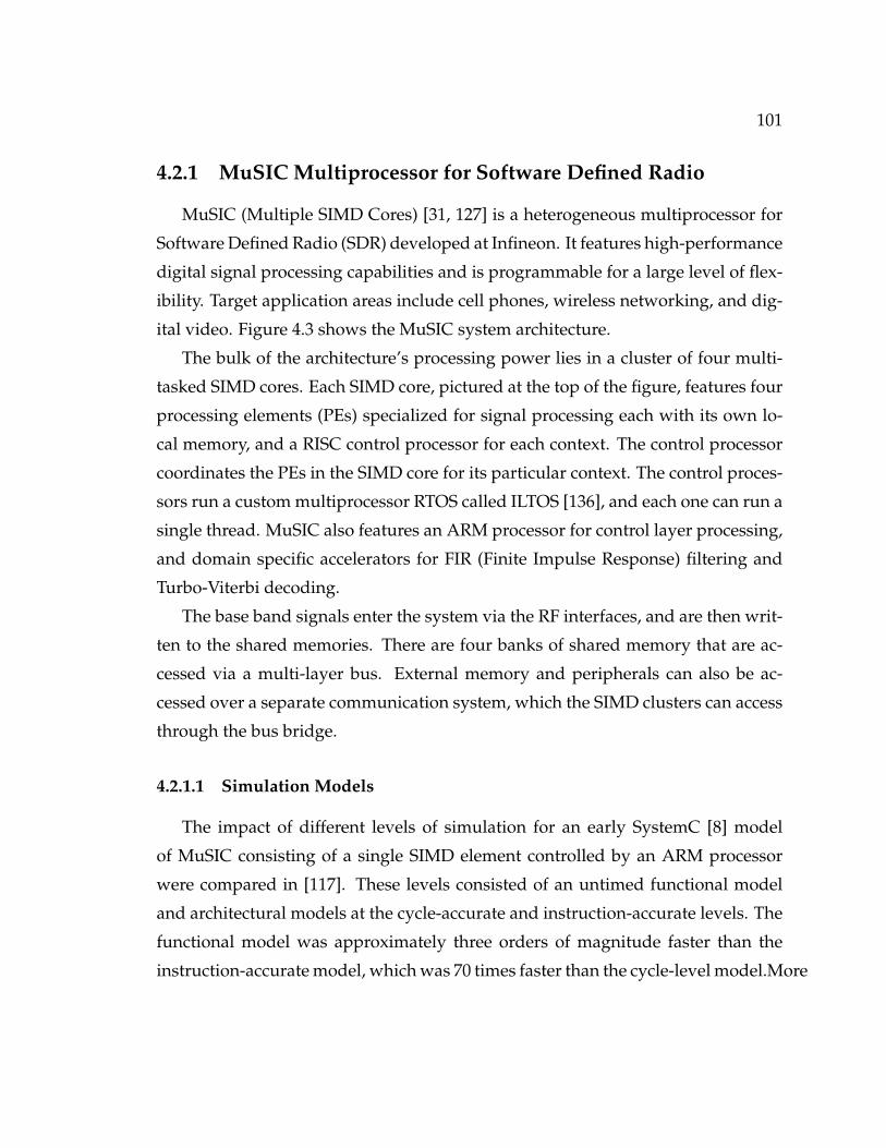
101
4.2.1 MuSIC Multiprocessor for Software Defined Radio
MuSIC (Multiple SIMD Cores) [31, 127] is a heterogeneous multiprocessor for
Software Defined Radio (SDR) developed at Infineon. It features high-performance
digital signal processing capabilities and is programmable for a large level of flex-
ibility. Target application areas include cell phones, wireless networking, and dig-
ital video. Figure 4.3 shows the MuSIC system architecture.
The bulk of the architecture’s processing power lies in a cluster of four multi-
tasked SIMD cores. Each SIMD core, pictured at the top of the figure, features four
processing elements (PEs) specialized for signal processing each with its own lo-
cal memory, and a RISC control processor for each context. The control processor
coordinates the PEs in the SIMD core for its particular context. The control proces-
sors run a custom multiprocessor RTOS called ILTOS [136], and each one can run a
single thread. MuSIC also features an ARM processor for control layer processing,
and domain specific accelerators for FIR (Finite Impulse Response) filtering and
Turbo-Viterbi decoding.
The base band signals enter the system via the RF interfaces, and are then writ-
ten to the shared memories. There are four banks of shared memory that are ac-
cessed via a multi-layer bus. External memory and peripherals can also be ac-
cessed over a separate communication system, which the SIMD clusters can access
through the bus bridge.
4.2.1.1 Simulation Models
The impact of different levels of simulation for an early SystemC [8] model
of MuSIC consisting of a single SIMD element controlled by an ARM processor
were compared in [117]. These levels consisted of an untimed functional model
and architectural models at the cycle-accurate and instruction-accurate levels. The
functional model was approximately three orders of magnitude faster than the
instruction-accurate model, which was 70 times faster than the cycle-level model.More

102
recently a SystemC-based cycle-accurate Virtual Prototype (VP) and an functional
simulator that is implements the ILTOS API have been developed.
The VP uses a cycle-level model for the control processor, which was created us-
ing CoWare’s Processor Designer software. It also contains a handwritten C/C++
model of the SIMD elements. The communication and memory systems are spec-
ified in SystemC at the cycle level. The virtual prototype is parameterizable in a
variety of ways including: the number of SIMD processors, enabling/disabling
different components, different levels of accuracy (and simulation speed) for dif-
ferent components, and the generation of a variety of statistics and performance
traces. This work uses execution traces for the SIMD control processors generated
by the virtual prototype. The functional model implements the ILTOS API on-top
of the Win32 API, and was ported to SystemC to support effective tracing and
timing annotation.
4.2.2 The XScale Microprocessor
The XScale Microprocessor [45, 52] is a scalar microprocessor implementing
the ARM instruction set[102] designed by Intel. Since its release there have been
multiple redesigns of it each with various speeds we focus on the PXA250 series of
the XScale that featured speeds of up to 400 MHz. It features a seven stage main
pipeline, an eight stage memory pipeline, dynamic branch prediction, and out of
order commit.
4.2.2.1 Simulation Models
For comparison this work used the ARM version of the Simplescalar tool set
[35], which is at: http://www.simplescalar.com/v4test.html. This was used be-
cause it was the only freely available ARM simulation environment distributed
with source code that had a model of the XScale microarchitecture that was found
at the time of this research. The source code was modified to generate traces, and

103
then the original version was used for performance comparisons.
4.3 Related Work
4.3.1 Software Tools
Profilers such as GPROF [13] provide performance numbers for functions in
terms of the number of times that they are executed and an estimate of the time
spent in each function. These operate at the function call level and the measured
times are based on sampling and so are not that accurate. Our approach examines
gets cycle-accurate measurements at the basic block level from actual execution
traces, and then annotates the original source code at the line level.
In [38], Cai et al. present an approach for system-level profiling, where a high-
level specification of an application described in SpecC [11] is profiled at the basic
block level to guide design space exploration. They also provide metrics for es-
timating delay and memory usage, both in general and also for specific architec-
tures. Our work is more focused on performance estimation and fast simulation
of software running on a particular processor, whereas this work deals with high
level decisions and refinement. As a result our approach is more detailed, but less
flexible in its scope. There are also a number of fine-grained profilers for debug-
ging embedded platforms. Companies offering these include: Mentor, Greenhills
Software, and ARM.
Micro-profiling from Meyr et al. [89], apply fine grained instrumentation to
software compiled to a three-address code intermediate representation. This al-
lows the capturing of cycle delays and memory accesses. In experiments it was
9.1x faster than an instruction accurate ISS-based execution, and achieves accu-
racy of within 80%, but it is unclear if this also applies to cycle accurate models.
Our work achieves greater speedup by operating at the source level. Our approach
is more accurate, but it does not handle memory accesses. An interesting question

104
is what level of granularity the simulation and annotation need to be done in order
to achieve reasonable accuracy with the maximum performance increase.
In 2008, Hwang, Abdi, and Gajski presented an approach for retargetable per-
formance estimation based on a compiler’s intermediate representation. This is
very similar to the micro-profiling work, but it doesn’t simulate memory traffic
and it is extended with a model of the host machine’s pipeline. It uses statistical
calculations to estimate branch mispredicts and cache misses (only for their tim-
ing impact). Our work is based on actual executions of the virtual prototype and
so automatically gets the benefit of these estimations. Furthermore our work has
been applied to a multiprocessor system, whereas there work has been applied to
a single processor communicating with hardware peripherals. Their accuracy is
similar to ours and they have a much faster annotation process4, but it was only
evaluated on a single application. Their work is retargetable since it is based on an
intermediate representation, but it may suffer inaccuracies based on architecture-
specific optimizations and specialized instruction sets. Also, their approach creates
annotated code based on the basic blocks generated by the compiler, whereas ours
operates on the actual source code, which makes our more useful for viewing the
performance of individual lines of code.
4.3.2 Performance Estimation for Embedded Systems
There has been much work in software performance estimation for embedded
systems. The POLIS project [26] generates source code based on Codesign Finite
State Machines (CFSMs) specified in Esterel [29]. It features performance estima-
tion [139] based on the CFSMs and also based on S-Graphs generated for the syn-
thesis process. The delays are then estimated based on values calculated by simu-
lating the processor on multiple benchmarks, or by specifying them in characteri-
zation files. For simple processors this approach had a maximum error magnitude
4This is due to our processing of actual execution traces and having the annotation frameworkwritten in Python.
105
of 25% accuracy. It is limited to synthesized code, whereas our technique is based
on the application code and achieves better accuracy.
In [28], the authors explore two different approaches for C Automatic Back-
wards Annotation (CABA): virtual compilation and object code based. The virtual
compilation approach compiles the source code to a generic RISC-like instruction
set and assigns delays to each instruction type based on the given microarchitec-
ture, with the annotations being written back to the original source code. Our
technique also annotates at the source level, but it differs in that it assigns delays
directly based on the results of simulation. The object-code based approach gen-
erates a C-level model based on the assembly from the compiled object code. This
requires significant effort in that the assembly language must be fully parsed and
then implemented in the C-simulation model. Our technique, aside from detect-
ing the class of synchronization instructions, is almost totally independent of the
assembly used and operates on the execution of basic blocks, yet it still achieves
good accuracy. Their work assumed ideal memory, and our work, while it does
not model memory, does factor in the timing impact of non-ideal memory based
on its measurements from the virtual prototype.
Fast Cycle Accurate Simulators with dynamic-translation such as those from
VaST[16] are similar to the object-code based approach, but can handle self modi-
fying code (such as an RTOS). These can reach speeds in the tens of MIPS range for
a single processor, but they are time consuming to build, modify, or retarget. Fur-
thermore, even this speed might be insufficient for large multiprocessors. CoW-
are’s processor designer can generate cache-compiled [116] simulators from pro-
cessors specified in the LISA language [123], but they are an order of magnitude
slower than the hand-customized VaST models. Section 1.4 has a more in depth
description of this type of work.
MESH [122] is a high level environment for exploring different multiprocessor
system on chip architectures. There are three layers to it: a logical layer consist-
ing of individual threads of execution from the application, a physical layer which

106
represents the processing elements and resources of the system, and a scheduling
and protocol layer which connects the logical layer to the physical layer. The logical
threads communicate with the intermediate layers by means of consume statements
which the schedulers turn into requests for physical resources on the physical el-
ements. For processors, the consume statements tend to be instruction counts of
one or more instruction types, and they are user-specified based on estimates or
simulations. We automatically annotate cycle delays obtained directly from target
source code running on the virtual prototype, and could easily extend our frame-
work to output instruction counts.
In [112] Moussa et al. present a methodology where software code are anno-
tated with cycle counts, which are estimated from examining the compiled exe-
cutable, and then multiplied by the frequency for simulation as part of a SystemC-
based Transaction-Level model of the architecture. They do not elaborate on how
the estimate occurs, but do say that there is not recompilation for new processors.
This suggests that the approach does not have high accuracy and is probably sim-
ilar to the approach used in POLIS [26] based on assigning a fixed cycle delay to
each type of instruction.
In [60], Densmore et al. characterize the communication architecture of a Xilinx
FPGA. These measured numbers are stored in a database, and then used to anno-
tate architecture models. Our work is complementary to this in that it focuses on
the computation aspect of performance annotation.
4.3.3 Worst-Case Execution Time Analysis
In 1995, Li and Malik, introduced techniques for doing worst case execution
time using integer linear programming [99, 100, 101]. While quite accurate, these
techniques did not scale to large programs or complicated microarchitectures. Since
then a wide number of improvements upon this approach have taken place. Wil-
helm et al. summarizes these improvements in [149]. The best known of these
comes from AbsInt [2], which combines abstract interpretation with integer linear

107
programming [148] to scale to real industrial examples. It does have the limitations
of only supporting simpler microarchitectures, and, in some cases, needing user-
annotations in the source code to improve accuracy. Our approach is not aimed
at worst case execution time, but could be used to gather statistics to drive such
approaches. Also, since we rely on measurements from an external model, we are
not limited by the complexity of the underlying microarchitectures.
4.3.4 Other Work
The FastVeri [4, 114] tool from InterDesign technologies is the work most simi-
lar to ours. It annotates delays based on analyzing the actual assembly language,
and also simulate IO and cache behavior. With this they claim to reach simula-
tion speeds of up to 100 Million cycles/second. FastVeri adds delays based on
an internal model of the architecture, whereas we measure delays taken from a
cycle-accurate virtual prototype. Their approach requires full parsing and anal-
ysis of assembly code, whereas we do not, making it much easier to retarget the
framework to new instructions sets and processors. Also, our approach supports
execution of multithreaded programs on a multi-processor RTOS, which FastVeri
appears not to do.
4.4 Discussion
This chapter has introduced the concept of annotation. It reviewed the basic
annotation tool flow and the platforms (and simulators) used for the annotation
experiments. It also reviewed related work. It has set the stage for the next two
chapters which detail uniprocessor and multiprocessor annotation respectively.

108
Chapter 5
Backwards Timing Annotation for
Uniprocessors
This chapter explains how source level timing backwards annotation is imple-
mented for a uniprocessor system running a single application. It reads in informa-
tion from application source files, debug-compiled assembly files, the disassem-
bled executable and performance traces from a cycle-accurate simulation model.
Based on this information the original source code is annotated with average de-
lays at the line level.
The next section (Section 5.1) presents the annotation algorithm in detail. Then,
Section 5.2 discusses the implementation and optimizations to it. After this results
annotation results are given and the chapter wrapped up.
5.1 Single Processor Timing Annotation Algorithm
After reading in the assembly, disassembly, and execution trace files the single
processor annotation algorithm has three main steps. First the assembly and disas-
sembly files are unified into a single description and then sliced into smaller code
blocks based on jumps (and branches) in the execution trace. Next, the execution

109
void main (int argc, char** argv) {...short *InputI = Alloc Mem(sizeof(short)*64); // line 23short *InputQ = Alloc Mem(sizeof(short)*64); // line 24...
Figure 5.1: Original example code.
trace is stepped through instruction by instruction and the timing annotations for
the individual blocks are calculated. When an execution of a block is finished that
annotation is added to its associated line. Finally, the annotated source code is
generated by adding the line-level annotations to the application’s original source
code. Figure 5.1 shows the source code excerpt that will be used to illustrate the
annotation process. It is two memory allocation statements. At each step in the
algorithm this code and its related files will be shown.
5.1.1 Construct Blocks and Lines
The initial step in the algorithm is constructing blocks and lines based on the
input files. This is broken up into two steps: (1) initial calculations and (2) block
slicing.
5.1.1.1 Initial Block and Line Calculations
The assembly for each source file is split up into functions, and these functions
are split up into lines, which are then split into blocks. The blocks are defined
based on the locations of the line numbers and the functions in the debug informa-
tion of the assembly, and the associated instruction addresses and sizes from the
disassembled executable. The instructions in the assembly and disassembly files
are aligned at the function labels present in both of them.
Figure 5.2(a) shows the initial unified assembly and disassembly. The shown
code is turned into three lines, where each line has a single block of code. The first

110
.Fmain:
.L1:00020200: sub r15, 2800020202: push r8..r1400020204: add r15, r15, -0x00cc
; ** line 2300020208: pgen2 r2, 70002020a: mov r3, 40002020c: mov r4, 20002020e: jl .FAlloc Mem00020212: nop00020214: nop00020216: nop00020218: nop0002021a: nop0002021c: nop0002021e: mov r12, r2
; **line 2400020220: pgen2 r2, 700020222: mov r3, 400020224: mov r4, 200020226: jl .FAlloc Mem0002022a: nop0002022c: nop0002022e: nop00020230: nop00020232: nop00020234: nop00020236: mov r11, r2
; ** line 25...
(a) ASM/DIS Before Slicing
.Fmain:
.L1:00020200: sub r15, 2800020202: push r8..r1400020204: add r15, r15, -0x00cc
; ** line 2300020208: pgen2 r2, 70002020a: mov r3, 40002020c: mov r4, 20002020e: jl .FAlloc Mem00020212: nop00020214: nop00020216: nop00020218: nop0002021a: nop0002021c: nop0002021e: mov r12, r2
; **line 2400020220: pgen2 r2, 700020222: mov r3, 400020224: mov r4, 200020226: jl .FAlloc Mem0002022a: nop0002022c: nop0002022e: nop00020230: nop00020232: nop00020234: nop00020236: mov r11, r2
; ** line 25...
(b) ASM/DIS After Slicing
Figure 5.2: Example Unified Assembly and Disassembly

111
Function Line Block Number Cycle Program Addressmain None 1 of 1 22429 0x00020200
22430 0x0002020222443 0x00020204
main 23 1 of 2 22444 0x0002020822445 0x0002020a22453 0x0002020c22454 0x0002020e22455 0x0002021222456 0x0002021422457 0x00020216
Alloc Mem N/A N/A 22465 ... JUMP to Alloc Mem...main 23 2 of 2 23016 0x0002021emain 24 1 of 2 23027 0x00020220
23028 0x0002022223029 0x0002022423030 0x0002022623031 0x0002022a23032 0x0002022c23039 0x0002022e
Alloc Mem N/A N/A 23040 ... JUMP to Alloc Mem...main 24 2 of 2 23361 0x00020236main 25 23362 0x00020238
Figure 5.3: Example Processor Execution Trace
line has no line number and represents the startup code for the main function. The
second and third lines are for the lines 23 and 24 in the executable.
5.1.1.2 Block Slicing at Jumps in the Execution Trace
The next step extracts the jump locations from the processor’s execution trace
and then slices the blocks at those points. The jump points are whenever an in-
struction in the execution trace is not immediately followed in the trace by its suc-
cessor. Slicing the blocks based on these boundaries guarantees that functions are
separated from the blocks that call them. This improves accuracy and helps the

112
annotator distinguish between known user code and unknown library code.
Figure 5.3 shows an excerpt of the processor trace used to slice the blocks. The
last two columns are the information in the processor trace giving the cycle and the
instruction of the address that begins execution in that cycle. A non-pipelined de-
lay model is used for instructions, so the current instruction ends execution when
its successor begins. The first three columns respectively indicate the function,
lines, and blocks that these instructions are associated with.
In this example, the blocks for lines 23 and 24 are both sliced where the ex-
ecution trace enters the Alloc Mem function. They are sliced three instructions
after the jump instruction going to Alloc Mem executes because of the processor’s
branch delay of three instructions. Figure 5.2(b) shows the unified assembly and
disassembly after the slicing.
5.1.2 Calculate Block and Line-Level Annotations
The next step records the absolute instruction and cycle counts of each execu-
tion of each block, and then adds these to the line level annotation.
5.1.2.1 Block Annotations
The delay of a block for a given execution is equal to the sum of the delays of all
of the instructions in that block for that execution. Its execution begins when the
block is entered, and ends when the block is left. Once a block is left its execution
count is incremented, and the number of cycles for that execution is added to its
line’s annotation. The cycle-count for an execution of a block is the cycle time of the
first instruction for that execution, subtracted from the cycle time of the instruction
following the last instruction of the block for that execution. For example, in Figure
5.3 the first block of line 23 begins execution at cycle 22,444 and the instruction
immediately following it begins at cycle 22,465. Thus, the block’s execution time is
21 cycles, and the second block in line 23 has an execution time of 11 cycles.

113
5.1.2.2 Line Annotations
Each time a block completes an execution, its annotation is added to its associ-
ated line. From this list two types of annotations are extracted for each line of code:
internal annotations and external annotations. Internal annotations are the cycles and
instructions of the blocks associated with that line of code. External annotations are
the cycles and instructions executed between source blocks in the execution, and
if they are between blocks from different lines they are associated with the earlier
block. Examples of these are calls to library functions or other functions where the
original source code is not available. This is consistent with the definitions for the
delays of blocks and instructions.
The internal and external annotations are summed together for each execution
of the line of code to get the cycle delay for that execution. The number of execu-
tions of a line is approximated as the largest number of executions of its internal
blocks at that point in the trace. This is generally true except for rare cases such
as recursive self loops and multiple statements written on a single line, which the
framework does not handle.
The delay annotations for each line can be calculated based on the cycle counts
for each execution. The delay annotation options include: average cycle delay,
maximum cycle delay, and minimum cycle delay. Since this work tries to match
the timing of the simulator and average cycle delays are used. If the goal was worst
(or best) case timing analysis then maximum (or minimum) cycle delay would be
used instead.
5.1.3 Generating Annotated Source Code
Once all of the line-level annotations have been calculated, the annotated source
code is generated. Figure 5.5 shows examples of the different annotation cases.
For the general case a line of code has the its cycle count written directly before
it in the annotated source file. For-loops and while-loops require special handling
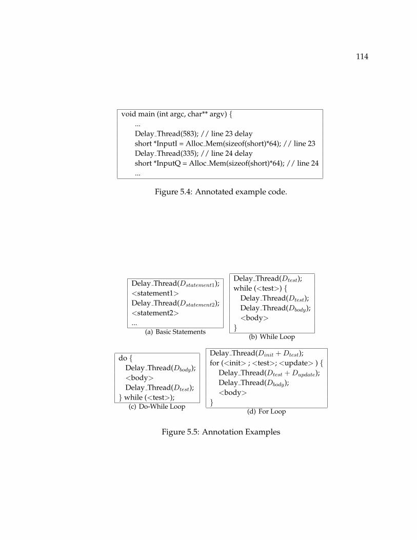
114
void main (int argc, char** argv) {...Delay Thread(583); // line 23 delayshort *InputI = Alloc Mem(sizeof(short)*64); // line 23Delay Thread(335); // line 24 delayshort *InputQ = Alloc Mem(sizeof(short)*64); // line 24...
Figure 5.4: Annotated example code.
Delay Thread(Dstatement1);<statement1>
Delay Thread(Dstatement2);<statement2>
...(a) Basic Statements
Delay Thread(Dtest);while (<test>) {
Delay Thread(Dtest);Delay Thread(Dbody);<body>
}(b) While Loop
do {Delay Thread(Dbody);<body>
Delay Thread(Dtest);}while (<test>);
(c) Do-While Loop
Delay Thread(Dinit + Dtest);for (<init> ; <test>; <update> ) {
Delay Thread(Dtest + Dupdate);Delay Thread(Dbody);<body>
}(d) For Loop
Figure 5.5: Annotation Examples

115
and are detailed below. Figure 5.5(a) shows this typical case where the two state-
ments, <statement1> and <statement2>, are annotated with their respective delays
of Dstatement1 and Dstatement2 cycles using the Delay Thread function.
For the example, we examine the single execution of line 23 pictured in Figure
5.3. The first block of line 23 is an internal delay of 21 cycles (i.e. 22,465 - 22,444
cycles). The call of Alloc Mem from line 23 takes 551 cycles (i.e. 23,016 - 22,444),
and is counted as an external delay. The second block of contributes an internal
delay of 11 cycles (i.e. 23,027 - 23,016 cycles). This leads line 23 to have an internal
delay of 32 cycles and a total delay of 582 cycles. Based on the processor trace, line
24 has a total delay of 335 cycles. Figure 5.4 shows the resultant annotated source
code for the sample lines.
5.1.3.1 Annotating While Loops
A while-loop consists of a test condition that guards the execution of the loop
body. If the condition evaluates to true, then the loop body executes once. This
process is repeated until the condition evaluates to false. If a while-loop executes
N times, then its condition evaluates N+1 times (N times to true, and 1 time to
false). Figure 5.5(b) shows an annotated while loop example. In the figure <test>
represents the test condition, and <body> is the loop body. Dtest and Dbody repre-
sent the cycle delays of the test and body blocks.
While-loops are detected by examining each line of the source code for lines
that begin with the while keyword, which can be preceded by whitespace and com-
ments. In this case, the condition delay is annotated before and after the while loop
statement. This exactly matches the real behavior of the while-loop.
Do-while loops do not need special handling because in them the test condition
executes the same number of times as the body does. Figure 5.5(c) shows an anno-
tated do-while loop. This is automatically generated with the default annotation
behavior.
116
5.1.3.2 Annotating For Loops
Like the while-loop, the for-loop has a test condition, but it adds an initialization
statement and an update statement. Each time the for-loop executes it runs the ini-
tialization statement once, and then checks the test condition. If the test condition
is true, then the loop body is executed once, otherwise the loop ends. After each
execution of the loop body the update code runs once and the condition is checked
again. This continues until the test condition evaluates to false. If a for-loop’s body
executes N times, then the test condition runs N+1 times and the update statement
runs N times.
Figure 5.5(d) shows an annotated for-loop. The sections for initialization, test-
ing, and update pieces of the for loop are denoted by <init>, <test>, and <update>
respectively. Dinit, Dtest, and Dupdate are their delays. The body of loop is <body>,
and Dbody is its delay.
For-loops are detected in the same manner as while-loops, except that the search
is for the for keyword. The initialization statement will always be the first block
executed in a for-loop. Given this, we subtract the delays for this block from the
for-loop’s line delay. The delay of the first block is annotated above the for-loop’s
line, and the line’s remaining delay is annotated directly below the for-loop’s line.
5.2 Implementation and Optimizations
For the annotation algorithm, its runtime complexity is equal to O(A + D + P),
where A is the number of instructions in assembly code, D is the number of instruc-
tion in the disassembled executable, and P is the number of entries in the processor
execution execution trace. This is true given that we hash the instruction accesses
so that they have constant access time. These numbers are by far dominated by the
size of the processor execution trace, and it turns out that memory usage and disk
storage must be optimized in order to handle realistically sized benchmark runs.
This section uses the below described variable definitions:

117
B - The set of blocks in the given system.
I(b) - The number of instructions for block b ∈ B.
L - The set of lines in the given system.
B(l) - The set of blocks that make up line l ∈ L.
Eb - The number of executions of blocks b ∈ B.
El - The number of executions of line l ∈ L.
EB - The number of blocks in the executed in the given system (∑
b∈B Eb).
EL - The number of executions of lines in the given system.
The next subsection (Section 5.2.1) describes different storage schemes for the
annotations and what their memory usage is. The subsection following (Section
5.2.2) it presents optimizations made to reduce the storage size for the processor
trace and also the time need to process it.
5.2.1 Memory Usage Optimizations
Since the annotations are stored for each block and also for each line, then the
overall annotation memory usage for storing each annotation separately is:
O(B + L + EB + EL)
This can quickly grow quite large for longer benchmarks. For example, assume
that there is a system with a million blocks executed and 2.5 × 10⁵ lines executed.
Assuming that storing each block execution takes 16 bytes of memory and that
storing each line execution 32 bytes of memory, this leads to a memory usage of
24×106 bytes1, which works out to approximately 23 Megabytes (24×106/(10242) =
22.89). However if 100 million blocks and 25 million lines had executed it would
consume over 2 Gigabytes of memory. Considering that some benchmarks execute
116× 1× 106 + 32× 2.5× 106 = 16× 106 + 8× 106 = 24× 106

118
billions of blocks, this is clearly not scalable. Two main approaches to deal with this
are presented below, and then other memory usage optimizations are discussed.
5.2.1.1 Optimization 1: Only store the current block annotations
Since the annotations are performed at the line level it is unnecessary to store
every block annotation. In fact, since block annotations are added to their given
line upon completion of an execution, only the current block’s execution data
needs to be stored. This leads to a memory usage of O(B+L+EL), and reduces the
example’s memory consumption by two-thirds to approximately 7.7 Megabytes
for annotation. This approach still stores all of the line annotations, and so still
may result excessive memory usage for larger benchmarks.
5.2.1.2 Optimization 2: Store combined line annotations
Given that the average (or maximum or minimum) of the cycle count of each
line’s executions is annotated to the original source code, it is not necessary to
store all of the annotations for each line. Thus, these annotations can be stored
in a combined manner. Specifically each line has the sum of they delays of its
executions, the number of times it was executed, and its minimum and maximum
execution delays. With this implementation the memory usage becomes O(B + L)
and is independent of the number of executions of lines and blocks, making it
scalable to arbitrarily large traces.
There are some drawbacks to using this line-level annotation storage. Since
a running average is kept for each line it is difficult to do path-based analysis or
calculate other statistics such as the median2. One could imagine using different
levels of optimized annotations to allow for a mixture of scalability and more de-
tailed statistics gathering.
2The optimized storage does track the minimum and maximum times for each line could beeasily be extended to track the standard deviation.

119
5.2.1.3 Other Memory Usage Optimizations
There are other optimizations that don’t impact the overall algorithmic storage
complexity, but significantly impact scalability. One of the first items is combining
what is being stored into a single number. For example, if each line is broken up
into internal cycles, external cycles, internal ignore cycles, external ignore cycles,
and pre-ignore cycles (used for the annotation of for-loops), then 5 numbers are re-
quired for each line. Except for the pre-ignore cycles, all of the others can be added
together to achieve a single number, which reduces the storage to 2 numbers. Also,
depending on the use of the annotator, instruction counts may be ignored which
halves the annotation overhead.
5.2.2 Trace Storage Optimizations
Because an execution trace of billions of cycles can be quite large it is impera-
tive to store such traces compactly. Furthermore, when dealing with traces gener-
ated from external tools there might be extraneous information in them that causes
them to be even larger. This section presents two optimizations that reduce the size
of stored traces.
For all cases the data traces are stored as a text file where, for each instruction
execution, the cycle upon which the instruction begins execution and the instruc-
tion’s address are stored. This leads to a usage of approximately 17 bytes per in-
struction execution (7 for address, 8 for cycle count, and 2 for spacing and new
lines). Which for 1 million instruction executions, leads to a storage overhead of
approximately 15 megabytes of disk space.
The first optimization is to store the trace file using differential encoding, where
only the difference between the current execution cycle and instruction and the
prior one are stored in the file. In practice, this reduces the number of characters
used for addresses and cycles to approximately 2 each. This means that the storage
overhead become less than 5 bytes per instruction execution (2 for address, 1 for

120
Table 5.1: Compression size results from small input set for MiBench[73]. Thesecond column shows the average number of bytes used for each line in thetrace for the base uncompressed non-differential encoding. The third, fourth, andfifth columns show the compression ratios respectively for: compressing the non-differential encoding, uncompressed differential encoding, and compressed differ-ential encoding.
Benchmark
Base Case (Bytes
/ Line)
Compressed Non-
Differential
Uncompressed
Differential
Compressed
Differential
adpcm.encode 17.11 4.35 4.16 217.09
adpcm.decode 16.88 4.39 4.09 243.17
dijkstra 17.41 5.47 4.20 552.31
patricia 18.23 4.22 4.22 54.42
rijndael.encode 16.95 3.59 4.15 570.85
rijndael.decode 16.93 3.54 4.16 649.41
sha 16.81 4.53 4.13 366.08
stringsearch* 15.09 4.62 3.56 218.71
average 16.93 4.34 4.08 359.01
Compression Ratio (Base Size / Compressed Size)
cycles, and 2 for spaces and new line), leading to a space reduction of over 3x.
The second optimization is using gzip to compress on the resultant trace files.
The compression ratio for the differentially encoded traces tends to be somewhat
better than the original traces because fewer types of characters are used, which
allows for greater compression. Table 5.1 shows the base size (per trace entry) for
the uncompressed entry and then shows the compression ratio for applying the
different optimizations. Compressing the base case and using differential encod-
ing have similar compression ratios of more than 4x. Whereas compressing the
differential coded trace reduces its size by 88x; this reduction is so dramatic be-
cause of the regularity of the trace, most address and cycle changes are the same
(4 and 1 respectively) and so the trace files are dominated by these numbers and
also the newline and space characters, leading to much better compression. Sec-
tion 5.3.4 investigates the impact of compression on execution runtime, and also
techniques for minimizing their impact on the runtime. .
There are other optimizations for storage that are possible, but were not im-

121
plemented. One is to pre-process the trace and only save the execution times of
the instructions from the assembly files and only save the overhead of the other
instructions. This could potentially significantly decrease the trace file size, but it
causes a loss of information, such as external function calls and instruction mem-
ory traffic, that might be needed to add extensions such as memory traffic to the
annotation. Another extension, is to run the annotator directly with the virtual pro-
totype that is generating the trace information. This would eliminate the need for
trace files, but would reduce the performance of the cycle level model and requires
that one has the capability to connect the annotator directly with the cycle-level
model.
5.3 Uniprocessor Annotation Results
Uniprocessor annotation was first evaluated on the same code running on the
same data in order to determine the baseline accuracy. Then it was evaluated on
the same code running on different data and different configurations, to see how
well it generalizes. Dhrystone [146] and some tests from MiBench[73] were evalu-
ated on the MuSIC and XScale platforms, and MuSIC also ran some internal tests
on a single control processor. Dhrystone [146] is a classic benchmark that fits in
cache and is used to calculate MIPS (Millions of Instructions Per Second) for typ-
ical integer workloads. MiBench[73] is a free set of representative embedded ap-
plications broken up into categories including: telecom, automotive, networking,
and office.
5.3.1 Simulation Platforms Evaluated
5.3.1.1 MuSIC: A Heterogeneous Multiprocessor for Software Defined Radio
The applications targeting a single SIMD control processor of MuSIC were com-
piled without optimization and then run on the virtual prototype. The annotated
122
source code was compiled with Microsoft Visual C++ 2005 and linked to the timed
functional simulator. The timed functional model was implemented using Sys-
temC 2.2, and it implemented delay annotation by using the timed wait function
in SystemC. The annotated source code running on the timed functional simulator
was compared to the same source code running on the virtual prototype in terms
of speed and accuracy. For non-disclosure purposes the numbers are given in a
relative manner. Unless otherwise noted, all of the experiments for the MuSIC
platform were run on a 2.0 GHz Core Duo laptop running Windows XP with 1 GB
of memory.
5.3.1.2 XScale Uniprocessor Platform
For the XScale processor tests, the annotation was compared against the ARM
[102] port of the Simplescalar[35] cycle-level out of order simulator using a config-
uration file matching the configuration of the XScale PXA250 architecture [45, 52].
The simulator was modified to generate execution traces for the annotator, and the
results from the annotator were compared against the unmodified version of the
simulator. Since this was only for uniprocessor annotation, the timing was stored
in a single static double precision floating point variable that was shared between
the annotated files via a common include file. All of the annotated code was com-
piled with -O2 optimizations using GCC version 4.1.1. Unless otherwise noted, all
XScale experiments were run on a 3.06 GHz Intel Xeon CPU with 512 KB cache and
3 GB of memory that runs Linux.
5.3.2 Results with Identical Data
5.3.2.1 MuSIC Results with Identical Data
Table 5.2 shows the results for the annotation of non-MiBench tests running
on a single MuSIC control processor. Aside from the Dhrystone 2.1 benchmark,
every benchmark is an internal test. The second column shows the error for an-
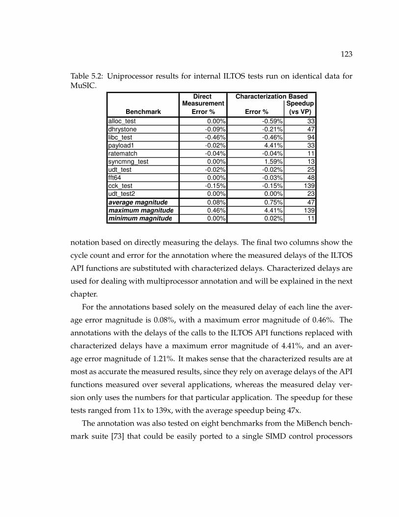
123
Table 5.2: Uniprocessor results for internal ILTOS tests run on identical data forMuSIC.
Direct
Benchmark
Measurement
Error % Error %
Speedup
(vs VP)
alloc_test 0.00% -0.59% 33
dhrystone -0.09% -0.21% 47
libc_test -0.46% -0.46% 94
payload1 -0.02% 4.41% 33
ratematch -0.04% -0.04% 11
syncmng_test 0.00% 1.59% 13
udt_test -0.02% -0.02% 25
fft64 0.00% -0.03% 48
cck_test -0.15% -0.15% 139
udt_test2 0.00% 0.00% 23
average magnitude 0.08% 0.75% 47
maximum magnitude 0.46% 4.41% 139
minimum magnitude 0.00% 0.02% 11
Characterization Based
notation based on directly measuring the delays. The final two columns show the
cycle count and error for the annotation where the measured delays of the ILTOS
API functions are substituted with characterized delays. Characterized delays are
used for dealing with multiprocessor annotation and will be explained in the next
chapter.
For the annotations based solely on the measured delay of each line the aver-
age error magnitude is 0.08%, with a maximum error magnitude of 0.46%. The
annotations with the delays of the calls to the ILTOS API functions replaced with
characterized delays have a maximum error magnitude of 4.41%, and an aver-
age error magnitude of 1.21%. It makes sense that the characterized results are at
most as accurate the measured results, since they rely on average delays of the API
functions measured over several applications, whereas the measured delay ver-
sion only uses the numbers for that particular application. The speedup for these
tests ranged from 11x to 139x, with the average speedup being 47x.
The annotation was also tested on eight benchmarks from the MiBench bench-
mark suite [73] that could be easily ported to a single SIMD control processors

124
Table 5.3: MiBench results for small and large data sets for the MuSIC platform.
Benchmark Error (%) Speedup Error (%) Speedup
adpcm.encode -1.67% 16 -0.70% 16
adpcm.decode -2.25% 16 -1.31% 40
dijkstra -12.63% 26 -17.46% 28
patricia -0.47% 82 -1.18% 66
rijndael.encode -1.26% 130 -2.96% 230
rijndael.decode -6.52% 159 -1.69% 234
sha 0.00% 1,031 0.00% 984
stringsearch 3.85% 15 -13.95% 29
average magnitude 2.80% 184 4.91% 203
maximum magnitude 12.63% 1,031 17.46% 984
minimum magnitude 0.00% 15 0.00% 16
Small Dataset Results Large Dataset Results
using the internal compiler. Table 5.3 shows the results using characterization-
based annotation. The first set of results are for the benchmarks running on the
small data set to exercise the functionality, and the second set of results is for the
larger data set that is more realistic. The maximum error magnitude is 17.5%, and
the average error magnitude is approximately 4%. The less accurate applications
use language constructs that are not well modeled in the annotator such as else-if,
and sometimes have multiple lines of code on the same physical line. There anno-
tated code has a wide range of speedup between 14x and 1030x, with an average
speedup of 194x. Table 5.4 shows the speedup of unannotated code running in the
framework compared to the virtual prototype, and how much faster it is than the
annotated code. The unannotated code has is between 160x and 130,000x faster
than the virtual prototype, which makes it on average almost 300x faster than the
annotated code with a maximum speedup of nearly 9,000x when compared to the
annotated code. There is a wide variation between these speedups because of the
granularity of the annotations, but this gives a rough boundary on the performance
potential of the annotated framework.

125
Table 5.4: MiBench speedup on MuSIC for no annotations versus the virtual pro-totype’s runtime, and then the slowdown caused by having annotations.
Benchmark
No Annotation
Speedup vs VP
Annotation
Slowdown vs No
Annotation
No Annotation
Speedup vs VP
Annotation
Slowdown vs No
Annotation
adpcm.encode 2,696 165 3,045 187
adpcm.decode 5,288 340 6,504 162
dijkstra 7,181 279 52,233 1,897
patricia 7,497 92 10,663 163
rijndael.encode 12,529 96 69,223 302
rijndael.decode 34,189 215 131,685 562
sha 6,214 6 25,539 26
stringsearch 160 11 2,089 73
average 9,469 151 37,623 421
maximum 34,189 340 131,685 1,897
Small Dataset Results Large Dataset Results
5.3.2.2 XScale Results with Identical Data
The Dhrystone benchmark and the MiBench applications run on MuSIC were
also evaluated on the XScale platform. The Dhrystone accuracy results running on
identical data are found in the bolded table entries in Table 5.10, it features error
magnitudes from 0.2% to 3.8%. The runtimes for Dhrystone on the XScale platform
are not compared since they are too small to be significant.
Both the small and large data sets of the MiBench applications from the pre-
vious section were run on the XScale platform and their full results are listed in
Tables 5.5 and 5.6 respectively. Table 5.7 summarizes the accuracy and speedup
for the MiBench applications. The error magnitude is within 11.1% and averages
3.8%. The speedup compared to the virtual prototype ranges from 100x to 5,900x
and averages 2,500x. The speedup is so large because annotation based on writing
to a shared variable is significantly faster than using delay calls to an event queue
like the MuSIC platform uses. Table 5.8 examines how much faster unannotated
native code is than the annotated code. It ranges from 1x to 8.3x faster, with the
average speedup being 2.1x.

126
Table 5.5: Full MiBench results for small data set for the XScale platform. Resultswere run on both the Simplescalar-ARM simulator (referred to as the virtual pro-totype) and on annotated source code produced from the framework.
Benchmark Cycles
Execution
Time (s) Cycles
Error vs.
Virtual
Prototype
Execution
Time (s)
adpcm.encode 125,343,711 193 119,174,880 -4.92% 0.121
adpcm.decode 91,935,992 109 85,766,470 -6.71% 0.2
dijkstra 163,031,337 193 162,711,423 -0.20% 0.039
patricia 170,500,688 198 169,819,746 -0.40% 0.073
rijndael.encode 85,648,291 105 81,244,318 -5.14% 0.04
rijndael.decode 84,033,024 94 93,281,916 11.01% 0.04
sha 55,428,098 61 54,963,544 -0.84% 0.017
stringsearch 520,785 0.64 515,253 -1.06% 0.006
Annotated CodeVirtual Prototype
Table 5.6: Full MiBench results for large data set for the XScale platform.
Benchmark Cycles
Execution
Time (s) Cycles
Error vs.
Virtual
Prototype
Execution
Time (s)
adpcm.encode 2,517,606,335 3004 2,397,704,255 -4.76% 2.29
adpcm.decode 1,824,189,623 2152 1,704,274,244 -6.57% 3.83
dijkstra 761450299 950 759,843,517 -0.21% 0.161
patricia 1,049,309,863 1296 1,045,457,551 -0.37% 0.41
rijndael.encode 891,186,440 1018 845,714,696 -5.10% 0.41
rijndael.decode 874,323,248 993 971,037,597 11.06% 0.41
sha 576,573,536 637 571,769,532 -0.83% 0.114
stringsearch 11,450,854 14 11,329,927 -1.06% 0.017
Virtual Prototype Annotated Code

127
Table 5.7: Summary of MiBench results for small and large data sets for the XScaleplatform.
Benchmark Error (%) Speedup Error (%) Speedup
adpcm.encode -4.92% 1,595 -4.76% 1,312
adpcm.decode -6.71% 545 -6.57% 562
dijkstra -0.20% 4,949 -0.21% 5,901
patricia -0.40% 2,712 -0.37% 3,161
rijndael.encode -5.14% 2,625 -5.10% 2,483
rijndael.decode 11.01% 2,350 11.06% 2,422
sha -0.84% 3,588 -0.83% 5,588
stringsearch -1.06% 107 -1.06% 824
average magnitude 3.78% 2,309 3.75% 2,781
maximum magnitude 11.01% 4,949 11.06% 5,901
minimum magnitude 0.20% 107 0.21% 562
Small Dataset Large Dataset
Table 5.8: MiBench speedup running on XScale for no annotations versus VP, andthen the slowdown of having annotations.
Benchmark
No Annotation
Speedup vs VP
Annotation
Slowdown vs No
Annotation
No Annotation
Speedup vs VP
Annotation
Slowdown vs No
Annotation
adpcm.encode 8042 5.0 2,704 2.1
adpcm.decode 4542 8.3 737 1.3
dijkstra 8773 1.8 12,500 2.1
patricia 2829 1.0 3,248 1.0
rijndael.encode 2625 1.0 2,545 1.0
rijndael.decode 2350 1.0 2,483 1.0
sha 5545 1.5 13,271 2.4
stringsearch 107 1.0 875 1.1
average 4351 2.6 4,795 1.5
maximum 8773 8.3 13,271 2.4
minimum 107 1 737 1.0
Small Results Large Results

128
Error Magnitudes for MiBench
0.00%2.00%4.00%6.00%8.00%
10.00%12.00%14.00%16.00%18.00%20.00%
adpc
m.e
ncode
adpc
m.d
ecode
dijks
tra
patri
cia
rijnd
ael.e
ncod
e
rijnd
ael.d
ecod
esh
a
strin
gsearc
h
aver
age
|Xscale Small Error|
|Xscale Large Error|
|MuSIC Small Error|
|MuSIC Large Error|
Figure 5.6: MiBench accuracy results for XScale and MuSIC annotations on thesame data.
5.3.2.3 Comparison between XScale and MuSIC results
Figure 5.6 shows the accuracy for the MiBench applications running on the
large and small data sets for both XScale and MuSIC. On average the XScale results
are slightly more accurate (3.8% vs. 3.9%). and it has a lower maximum error
magnitude (11.1% vs 17.5%).
Figure 5.7 shows the speedups of the annotated source code for the MiBench
experiments on the XScale and MuSIC. The average speedup of the XScale is sig-
nificantly greater (2250x vs. 190x) because it simply uses a static global variable
for storing annotations. For Music the annotations are implemented by calls to the
wait function in SystemC, which is much less efficient.

129
Annotation Speedup on MiBench
1
10
100
1,000
10,000
adpc
m.e
ncode
adpc
m.d
ecode
dijks
tra
patri
cia
rijnd
ael.e
ncod
e
rijnd
ael.d
ecod
esh
a
strin
gsearc
h
aver
age
XScale Small Speedup
XScale Large Speedup
MuSIC Small Speedup
MuSIC Large Speedup
Figure 5.7: MiBench speedup results for XScale and MuSIC annotations on thesame data (log scale).
5.3.3 Results with Different Data
5.3.3.1 MuSIC Results with Different Data
The results so far mentioned are quite accurate because, since the same data is
used, the annotated code takes the same path through the program’s control flow
graph as the original run did. To better evaluate the performance it is necessary to
compare the accuracy of the annotated code running on different data and different
control flows than those used in the characterization. This section presents the
results for the tests that were easily modified to have different execution flows
either by changing constants or running them on different input files.
The Dhrystone benchmark was run with loop counts of 1, 10, 100, 500, and 1000
to generate annotated source files. Each annotated result was then run on all of the
loop counts to evaluate the data-dependence accuracy of the annotation. Table 5.9
shows these error results. The single loop count results in the first row have an
average error magnitude of 25% and a maximum error magnitude of 47%. These

130
Table 5.9: Annotation error for Dhrystone benchmark for the MuSIC platformtrained and run on different numbers of iterations. The rows indicate the numberof iterations to generate the annotated sources. The columns indicate the numberof iterations run on the annotated sources. The last row and column indicate theaverage error magnitudes for the testing columns and training rows respectively.The bolded values in the table indicate the error for having the same iteration countfor generation and testing.
Generating Count /
Testing Count 1 10 100 500 1000
Average
Magnitude
1 -0.1% 5.3% 28.4% 43.7% 46.9% 24.9%
10 -1.2% -0.6% 2.4% 4.4% 4.9% 2.7%
100 -0.8% -1.1% -2.2% -2.8% -2.9% 1.9%
500 -0.4% -0.8% -2.4% -3.2% -3.4% 2.1%
1000 -0.2% -0.7% -2.3% -3.3% -3.5% 2.0%
Average Magnitude 0.6% 1.7% 7.5% 11.5% 12.3% 6.7%
large errors are to be expected, because the annotations are only based on the initial
execution where the code is loaded into the instruction cache. The loop count
of 10 has reduced error, but is still biased from the initial cache misses. The last
three loop counts have much better error numbers, with average error magnitudes
under 2.1%, and maximum error magnitudes of under 3.5%.
We also modified the size of the file that the internal test application udt test
writes out and then reads in, and produced annotated source files trained by these
numbers. The sizes were: 15, 31, 63, 127, and 255. In this case the maximum error
magnitude was 4.9%, and the average error magnitude was 1.7%.
For all of the mentioned MiBench tests, except for stringsearch which initialized
data in the source code, the large data set trained annotated code was run on the
small data sets, and vice versa. For the large data set trained code the average and
maximum magnitudes were 4.6% and 17.5%, and the magnitudes were 2.9% and
12.6% for the small data set trained code.

131
5.3.3.2 XScale Results with Different Data
The Dhrystone benchmark was run with loop counts of 1, 10, 100, 500, and 1000
to generate annotated source files. Each annotated result was then run on all of the
loop counts to evaluate the data-dependence accuracy of the annotation. Table
5.10 shows these error results. The single loop count results in the first row have
an average error magnitude of 77% and a maximum error magnitude of 145%.
These large errors are to be expected, because the annotations are only based on
the initial execution where the code is loaded into the instruction cache. The last
three loop counts have much better error numbers, with average error magnitudes
of 3.1% and below, and maximum error magnitudes of 3.8% and below.
For all of the mentioned MiBench tests, except for stringsearch which initialized
data in the source code, the large data set trained annotated code was run on the
small data sets, and vice versa. In both cases the maximum error magnitude stayed
within 0.1% of the annotated code running on the same data. The small data set
trained code running on the large data set had an average error magnitude of 6.3%,
which increases the average error magnitude by 2.7 percentage points. The large
data set trained code running on the small data set had an average error magnitude
of 4.7%, and which is a 1 percentage point increase in average error magnitude.
5.3.4 Annotation Framework Runtime
For the small dataset running on MuSIC the annotation time ranges from 1x
to 3.5x the virtual prototype’s simulation time, and from 0.5x to 1.5x for when the
processor trace is cached (i.e. preprocessed). For the large dataset of MiBench for
MuSIC the annotation runtime ranged from 1x to 2.9x that of the virtual proto-
type’s runtime (the cached results were not calculated for these).
The XScale uniprocessor annotation runtime numbers are more relevant than
those from MuSIC since they are absolute instead of relative. Table 5.11 shows the
annotation framework runtime of Mibench running on the Millenium cluster of
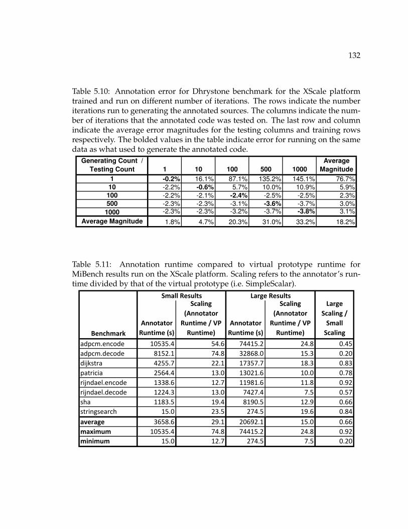
132
Table 5.10: Annotation error for Dhrystone benchmark for the XScale platformtrained and run on different number of iterations. The rows indicate the numberiterations run to generating the annotated sources. The columns indicate the num-ber of iterations that the annotated code was tested on. The last row and columnindicate the average error magnitudes for the testing columns and training rowsrespectively. The bolded values in the table indicate error for running on the samedata as what used to generate the annotated code.
Generating Count /
Testing Count 1 10 100 500 1000
Average
Magnitude
1 -0.2% 16.1% 87.1% 135.2% 145.1% 76.7%
10 -2.2% -0.6% 5.7% 10.0% 10.9% 5.9%
100 -2.2% -2.1% -2.4% -2.5% -2.5% 2.3%
500 -2.3% -2.3% -3.1% -3.6% -3.7% 3.0%
1000 -2.3% -2.3% -3.2% -3.7% -3.8% 3.1%
Average Magnitude 1.8% 4.7% 20.3% 31.0% 33.2% 18.2%
Table 5.11: Annotation runtime compared to virtual prototype runtime forMiBench results run on the XScale platform. Scaling refers to the annotator’s run-time divided by that of the virtual prototype (i.e. SimpleScalar).
Benchmark
Annotator
Runtime (s)
Scaling
(Annotator
Runtime / VP
Runtime)
Annotator
Runtime (s)
Scaling
(Annotator
Runtime / VP
Runtime)
Large
Scaling /
Small
Scaling
adpcm.encode 10535.4 54.6 74415.2 24.8 0.45
adpcm.decode 8152.1 74.8 32868.0 15.3 0.20
dijkstra 4255.7 22.1 17357.7 18.3 0.83
patricia 2564.4 13.0 13021.6 10.0 0.78
rijndael.encode 1338.6 12.7 11981.6 11.8 0.92
rijndael.decode 1224.3 13.0 7427.4 7.5 0.57
sha 1183.5 19.4 8190.5 12.9 0.66
stringsearch 15.0 23.5 274.5 19.6 0.84
average 3658.6 29.1 20692.1 15.0 0.66
maximum 10535.4 74.8 74415.2 24.8 0.92
minimum 15.0 12.7 274.5 7.5 0.20
Small Results Large Results

133
Linux computers at Berkeley3. The annotator runtimes are between 13x and 75x
that of the virtual prototype for the small data set, and the range is from 8x to 25x
for the large data set. These are larger than those for MuSIC because the simulator
used for the virtual prototype is much simpler (uniprocessor with a single ded-
icated memory, vs. multiprocessor with a complicated shared memory system),
and thus much faster. An interesting point is that the runtime scale actually de-
creases from the small data set to that of the large data set. If the scale stayed the
same for multiple data points this would imply a linear relation to the runtime of
the VP, but more experiments need to be done to evaluate this runtime.
It is important to note that there are many inefficiencies in the annotation frame-
work. First off, since compressed trace files are used this adds some overhead.
Then there is the fact that this is written in Python, which is an interpreted lan-
guage, whereas a native version should be significantly faster. Finally, it could be
integrated to run directly with the simulator (either compiled directly, or possibly
communicating via sockets on a different computer), which would alleviate much
of the current overhead. Next we examine the impact of using compressed trace
files.
5.3.4.1 Impact of Compression and Caching on Annotator Runtime
In order to reduce the execution overhead of the trace pre-processing, the re-
sults are saved in compressed files (one for each processor’s trace). Also, the jump
points and the lengths of the traces for each processor are saved in files. When
the annotator is run the modification time of the original processor trace file is
compared with those from the processed files, and if it is older, then only the pre-
processed files are read out. We refer to this as caching trace files.
To determine the impact of using caching and gzip compression we compared
the execution times of the annotation framework using different combinations of3These computers also feature a 3 GHz Xeon Processors with 3 GB of Memory, but they
each have 1 MB of Cache and feature a high-speed filesystem. For more information go to:http://www.millennium.berkeley.edu/PSI/index.html

134
Table 5.12: Runtime impact of compression and caching on the annotation processfor the small dataset of MiBench [73]. Caching runtime reduction is the runtime ofthe cached version subtracted from the uncached version and then divided by theruntime of the uncached version. Compression runtime increase is the runtime ofthe uncompressed version subtracted from the runtime of the compressed versionand then divided by the runtime of the uncompressed version.
Benchmark
Compressed
Trace
Uncompressed
Trace Uncached Trace Cached Trace
adpcm.encode 13.39% 12.95% 3.57% 3.04%
adpcm.decode 13.69% 13.45% 3.93% 3.64%
dijkstra 17.03% 20.34% 1.83% 6.07%
patricia 32.40% 39.33% 5.15% 17.17%
rijndael.encode 26.15% 31.94% 1.11% 9.72%
rijndael.decode 27.87% 31.81% 3.79% 9.78%
sha 21.21% 20.36% 4.70% 3.58%
stringsearch 14.86% 15.66% 2.10% 3.07%
average 20.82% 23.23% 3.27% 7.01%
Caching Runtime Reduction Compression Runtime Increase
caching and compression. Table 5.12 shows these results. The cached runtime re-
duction can be thought of as the percentage of time used for trace reading, which
takes 20.8% and 23.2% of the runtime on average for the compressed and uncom-
pressed traces. The average runtime increase for using compression on cached and
uncached traces an additional runtime of 3.3% and 7% respectively. Furthermore,
each trace is read through twice in the uncached version, so the runtime values
are roughly doubled here. This makes it clear that the trace reading time is a large
bottleneck for performance, but the compression is not.
5.3.5 Analysis
5.3.5.1 MuSIC Analysis
On MuSIC, the annotated uni-processor applications running on the same data
the error magnitude as within 18%, with an average error magnitude of 4%. Mul-
tiple factors contribute to error in the annotated code. Since some programs rely

135
on assembly programs running on the SIMD elements, and these are not modeled
in the timing annotated simulator, some accuracy is lost. Finally, the handling of
for-loops is inexact because the first condition check of the loop is currently not
counted.
For the applications running on different data on the MuSIC architecture, only
the Dhrystone benchmark had significantly reduced accuracy. The generally excel-
lent accuracy is somewhat misleading. This work only annotated measured timing
results from the virtual prototype, and the tests run are relatively simple and with
very regular memory access patterns. Thus most of the programs fit into the in-
struction cache, and there is little contention for the shared memory. For more
complicated examples that are impacted by contention in the communication sys-
tem or caching effects, the accuracy is expected to decrease.
The speedup of the annotated code MuSIC compared to the virtual prototype
was 10x to 1000x. Tests that call external functions (e.g. printf) or utilize the SIMD
or co-processors have greater speedup since these features are cheap or not mod-
eled in the timed simulator. Another way to think of this is that the number of
instructions per annotation is less. Each delay annotation slows down the perfor-
mance of the simulator, since it places an event on the SystemC event queue and
returns control to the SystemC scheduler. While measuring cycles-per-second of
an event based simulator is not fully fair, it does show how the annotated code
running on the functional simulator performs compared to the virtual prototype.
It is important to note that little effort has been made to optimize the speed of
the functional simulator. In addition to speeding up the code, performance can be
increased by combining annotations in straight line application code and also by
experimenting with different compilation options. Finally, switching to a commer-
cial SystemC simulator may further increase the annotation performance.
136
5.3.5.2 XScale Analysis
For the MiBench applications running on the same data on the XScale microar-
chitecture, the error magnitude was within 11.1% with an average of 3.8%. For
Dhyrstone, the error ranged from 0.2% to 3.8%. The accuracy here is very similar
to those of MuSIC. Interestingly, there is more variation for the Dhyrstone results,
but less variation on the MiBench.
For different data, the XScale had worse results than MuSIC for both Dhyr-
stone and the MiBench applications. On average the Dhrystone on XScale had an
average error magnitude of 18.2%, significantly worse than the that of MuSIC. For
MiBench the increase in error magnitudes was also worse than on MuSIC, but had
a very small change. We believe that this large impact on the XScale is because
it has a more complicated memory system and a longer pipeline than the MuSIC
control processors.
For the XScale the annotated code ran on average 2,300x faster than code run-
ning on Simplescalar, and its slowdown compared to native execution is 2x. The
annotation here is significantly more efficient than in the case of MuSIC because it
is done with a local variable and not using the SystemC event queue. Also, since
the operating system of the target and host are both Linux, there is no need to
implement the interface functions for the operating system.
5.4 Discussion
This chapter presented a technique for source level timing annotation for a sin-
gle processor application. This promising technique is easily retargeted to other
architectures. It was implemented for a heterogenous multiprocessor from Infi-
neon and then ported to the XScale microarchitecture. The next chapter extends
this approach to multiprocessor annotation. In particular, it describes different is-
sues encountered when moving to multiprocessor annotation and how to handle
them.

137
Chapter 6
Backwards Timing Annotation for
Multiprocessors
The previous chapter presented a method for the automated source-level tim-
ing annotation of programs running on a single processor. This chapter expands
this method to the multiprocessor realm. The first attempt was to directly unify
the measurements from each processor and annotate the code that way, but this
caused some problems. This chapter presents an example which illustrates these
problems and then explains solutions to these problems that do not rely on con-
currently analyzing multiple traces. This yields a scalable, accurate, and flexible
annotation technique.
The next section (Section 6.1) presents a motivating example that illustrates the
need for special handling of startup delays and inter-processor communication.
The handling of startup delays and inter-processor communication are detailed in
Sections 6.2 and 6.3 respectively. Section 6.4 presents results on a number multi-
processor applications, and then the chapter is wrapped up.

138
Line # Source Code20 void main(void) {21 thread* next thread;22 next thread = Create Thread(main);23 Wait Exit(next thread);24 Exit();}
Figure 6.1: Thread test example: initial unannotated code.
6.1 Introduction
It is important to note that this annotation technique has a few restrictions.
Also, it assumes an SMP (Symmetric Multi-Processor) RTOS running a single pro-
gram on the system where there is no preeemption. Furthermore, where each
processor can only run a single thread and new threads are allocated to unused
processors.
6.1.1 Motivating Example
Figure 6.1 shows the source code and line numbers for a multi-threaded ap-
plication called thread test1. This example instantiates a new thread running the
same main function by calling the Create Thread function and then it waits for the
child thread to exit through the Wait Exit function. Once the child thread exits, the
original thread exits by calling the Exit function. If the platform running this ap-
plication supported an arbitrary number of threads, then it would execute forever
(or until it ran out of memory). However, for this example, each CPU can only run
one thread, and the system has five CPUs. Thus, when Create Thread is called for
the fifth time a thread is not created and a null pointer is returned. Then, when
the fifth thread calls the Wait Exit function on the null pointer it immediately ex-
its. Given this and the below-specified delays, different annotation strategies are
1Thread test is taken from an internal multiprocessor tests described in Section 6.4.
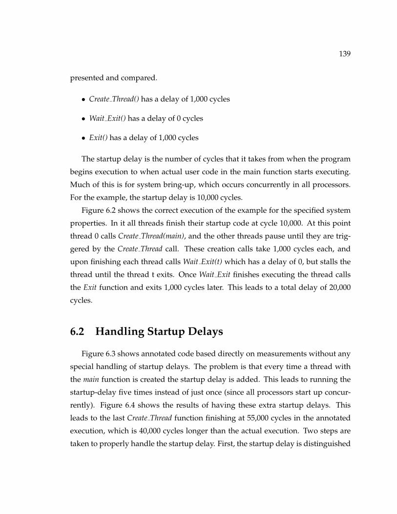
139
presented and compared.
• Create Thread() has a delay of 1,000 cycles
• Wait Exit() has a delay of 0 cycles
• Exit() has a delay of 1,000 cycles
The startup delay is the number of cycles that it takes from when the program
begins execution to when actual user code in the main function starts executing.
Much of this is for system bring-up, which occurs concurrently in all processors.
For the example, the startup delay is 10,000 cycles.
Figure 6.2 shows the correct execution of the example for the specified system
properties. In it all threads finish their startup code at cycle 10,000. At this point
thread 0 calls Create Thread(main), and the other threads pause until they are trig-
gered by the Create Thread call. These creation calls take 1,000 cycles each, and
upon finishing each thread calls Wait Exit(t) which has a delay of 0, but stalls the
thread until the thread t exits. Once Wait Exit finishes executing the thread calls
the Exit function and exits 1,000 cycles later. This leads to a total delay of 20,000
cycles.
6.2 Handling Startup Delays
Figure 6.3 shows annotated code based directly on measurements without any
special handling of startup delays. The problem is that every time a thread with
the main function is created the startup delay is added. This leads to running the
startup-delay five times instead of just once (since all processors start up concur-
rently). Figure 6.4 shows the results of having these extra startup delays. This
leads to the last Create Thread function finishing at 55,000 cycles in the annotated
execution, which is 40,000 cycles longer than the actual execution. Two steps are
taken to properly handle the startup delay. First, the startup delay is distinguished
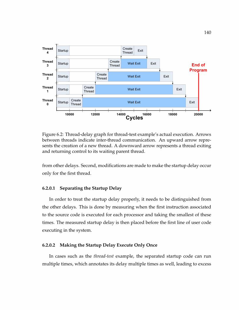
140
Startup
Startup
Startup
Startup
Startup
Create
Thread
Create
Thread
Create
Thread
Create
Thread
Create
ThreadExit
Exit
Exit
Exit
Exit
10000 12000 14000 16000 18000 20000
Thread
4
Thread
3
Thread
2
Thread
1
Thread
0Wait Exit
Wait Exit
Wait Exit
Wait Exit
End of
Program
Cycles
Figure 6.2: Thread-delay graph for thread-test example’s actual execution. Arrowsbetween threads indicate inter-thread communication. An upward arrow repre-sents the creation of a new thread. A downward arrow represents a thread exitingand returning control to its waiting parent thread.
from other delays. Second, modifications are made to make the startup delay occur
only for the first thread.
6.2.0.1 Separating the Startup Delay
In order to treat the startup delay properly, it needs to be distinguished from
the other delays. This is done by measuring when the first instruction associated
to the source code is executed for each processor and taking the smallest of these
times. The measured startup delay is then placed before the first line of user code
executing in the system.
6.2.0.2 Making the Startup Delay Execute Only Once
In cases such as the thread-test example, the separated startup code can run
multiple times, which annotates its delay multiple times as well, leading to excess
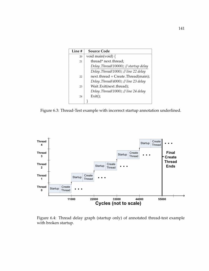
141
Line # Source Code20 void main(void) {21 thread* next thread;
Delay Thread(10000); // startup delayDelay Thread(1000); // line 22 delay
22 next thread = Create Thread(main);Delay Thread(4000); // line 23 delay
23 Wait Exit(next thread);Delay Thread(1000); // line 24 delay
24 Exit();}
Figure 6.3: Thread-Test example with incorrect startup annotation underlined.
Startup
Startup
Startup
Create
Thread
Create
Thread
Create
Thread
11000 22000 33000 44000 55000
Thread
4
Thread
3
Thread
2
Thread
1
Thread
0
StartupCreate
Thread
StartupCreate
Thread
Cycles (not to scale)
Final
Create
Thread
Ends
Figure 6.4: Thread delay graph (startup only) of annotated thread-test examplewith broken startup.
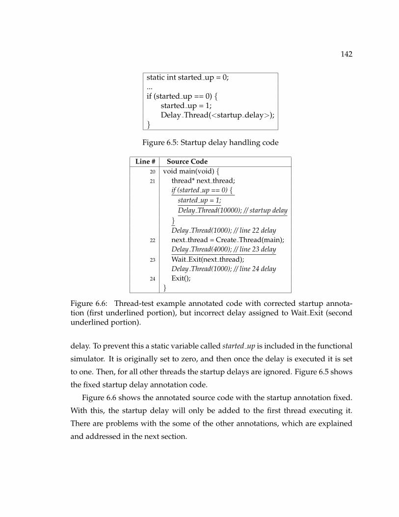
142
static int started up = 0;...if (started up == 0) {
started up = 1;Delay Thread(<startup delay>);
}
Figure 6.5: Startup delay handling code
Line # Source Code20 void main(void) {21 thread* next thread;
if (started up == 0) {started up = 1;Delay Thread(10000); // startup delay}Delay Thread(1000); // line 22 delay
22 next thread = Create Thread(main);Delay Thread(4000); // line 23 delay
23 Wait Exit(next thread);Delay Thread(1000); // line 24 delay
24 Exit();}
Figure 6.6: Thread-test example annotated code with corrected startup annota-tion (first underlined portion), but incorrect delay assigned to Wait Exit (secondunderlined portion).
delay. To prevent this a static variable called started up is included in the functional
simulator. It is originally set to zero, and then once the delay is executed it is set
to one. Then, for all other threads the startup delays are ignored. Figure 6.5 shows
the fixed startup delay annotation code.
Figure 6.6 shows the annotated source code with the startup annotation fixed.
With this, the startup delay will only be added to the first thread executing it.
There are problems with the some of the other annotations, which are explained
and addressed in the next section.

143
6.3 Handling Inter-Processor Communication
Inter-processor communication requires special handling because the proces-
sors’ execution traces are all handled independently. First, an example of why spe-
cial handling is needed is presented. Then, the techniques of ignoring the delays
of inter-processor communication function in the annotation calculations and then
adding in characterized delays for the inter-processor communication functions at
simulation are presented. Finally, reasons for why the traces are not concurrently
analyzed are presented.
6.3.1 Example with Inter-processor Communication Problems
If the delays of the calls to Wait Exit are directly measured and averaged, then
it ends up being assigned a delay of 4,000 cycles2; which leads to the annotated
code shown in Figure 6.6. Figure 6.7 shows the execution trace resulting from the
annotated code , where the dark Extra Wait blocks indicate the extra delay added
to the Wait Exit function calls. In this case, the extra delay only impacts thread 4’s
delay causing the total annotated delay of the program to be 4,000 cycles too large.
6.3.2 Ignoring Inter-processor Communication Delays
Since the line-level annotations are calculated independently for each proces-
sor, the inter-processor communication delays are counted on both sides of the
communication, leading to double counting. This is dealt with by ignoring the
delays of multiprocessor functions in the RTOS API. Once a multiprocessor RTOS
API function is called, annotation calculations are ignored until an internal piece
of code is executed. This is the same as ignoring the RTOS API function, as long
as none of the annotated code is called by the function, which is a reasonable as-
sumption. Figure 6.8 shows the example code with the delays of Wait Exit and
2Given this behavior the wait time for threads 0 to 4 respectively are: 8000, 6000, 4000, 2000, and0 cycles; with the average wait time being 4,000 cycles.
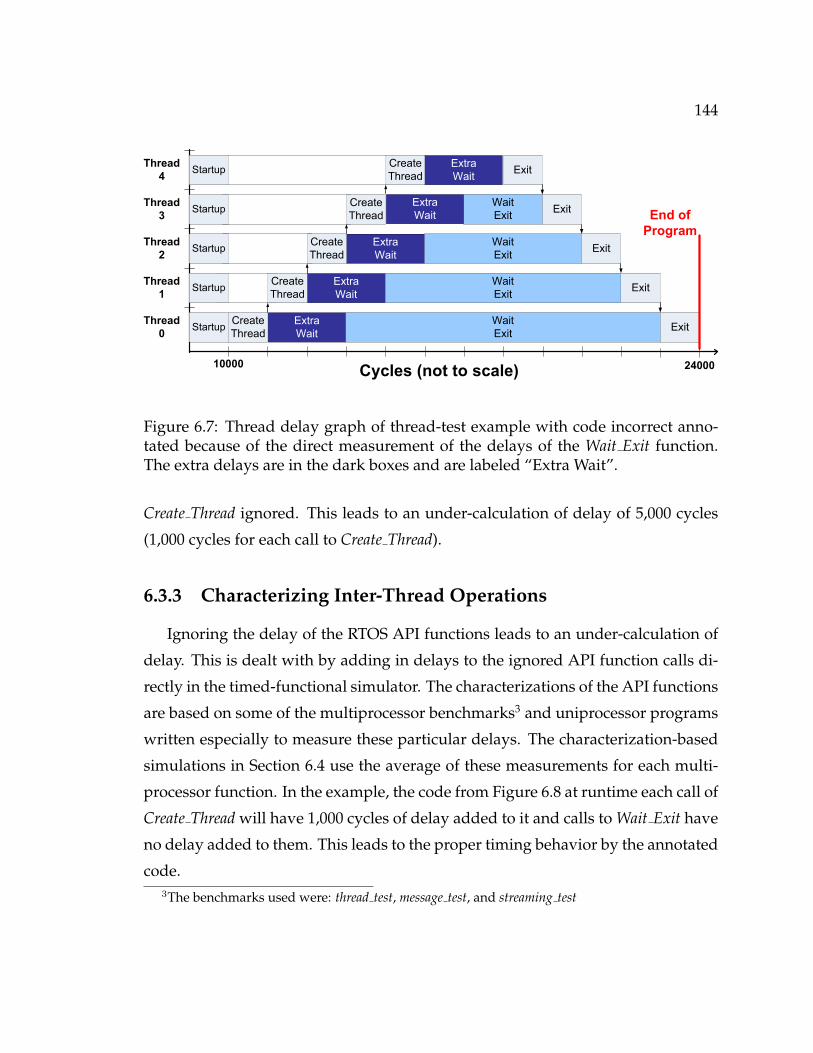
144
Startup
Startup
Startup
Startup
Startup
Create
Thread
Create
Thread
Create
Thread
Create
Thread
Create
ThreadExit
Exit
Exit
Exit
Exit
10000
Thread
4
Thread
3
Thread
2
Thread
1
Thread
0
Wait
Exit
Wait
Exit
Wait
Exit
Wait
Exit
End of
Program
Cycles (not to scale)
Extra
Wait
Extra
Wait
Extra
Wait
Extra
Wait
Extra
Wait
24000
Figure 6.7: Thread delay graph of thread-test example with code incorrect anno-tated because of the direct measurement of the delays of the Wait Exit function.The extra delays are in the dark boxes and are labeled “Extra Wait”.
Create Thread ignored. This leads to an under-calculation of delay of 5,000 cycles
(1,000 cycles for each call to Create Thread).
6.3.3 Characterizing Inter-Thread Operations
Ignoring the delay of the RTOS API functions leads to an under-calculation of
delay. This is dealt with by adding in delays to the ignored API function calls di-
rectly in the timed-functional simulator. The characterizations of the API functions
are based on some of the multiprocessor benchmarks3 and uniprocessor programs
written especially to measure these particular delays. The characterization-based
simulations in Section 6.4 use the average of these measurements for each multi-
processor function. In the example, the code from Figure 6.8 at runtime each call of
Create Thread will have 1,000 cycles of delay added to it and calls to Wait Exit have
no delay added to them. This leads to the proper timing behavior by the annotated
code.3The benchmarks used were: thread test, message test, and streaming test

145
Line # Source Code20 void main(void) {21 thread* next thread;
if (started up == 0) {started up = 1;Delay Thread(10000);}
22 next thread = Create Thread(main);23 Wait Exit(next thread);
Delay Thread(1000); // line 24 delay24 Exit();}
Figure 6.8: Thread-test example with corrected startup annotation, and with thedelays of Wait Exit and Create Thread ignored.
6.3.4 Handling Pipelining
Since most microprocessors are pipelined and the trace only gives one delay
number for each instruction instance’s execution, the linear delay model used is
inexact. Thus, if the current instruction execution is a synchronization instruction
that must stall and there are instructions after it in the pipeline, then the synchro-
nization delay of the current instruction execution may be allocated to its successor.
If this happens and the successor is associated with the next line, then the synchro-
nization delay will be associated with the next line, and thus will not be ignored
by the annotation framework.
While this seems like an unlikely case it did occur for the MuSIC processor be-
cause it has intrinsic instructions that directly some of implement the synchroniza-
tion functions in a single instruction, whereas function calls typically have multiple
clean up instructions after them which helps avoids this problem. These intrinsics
resulted in the synchronization delay for some calls of Wait Event to be assigned
to the instruction after it, and thus it wasn’t ignored for the delay calculation of
that line. Figure 6.9 shows the resultant source code that results from having the
measured wait delay added to after the Wait Exit line and Figure 6.10 shows its

146
Line # Source Code20 void main(void) {21 thread* next thread;
if (started up == 0) {started up = 1;Delay Thread(10000); // startup delay}
22 next thread = Create Thread(main);23 Wait Exit(next thread);
Delay Thread(4000); // line 24 extra delayDelay Thread(1000); // line 24 delay
24 Exit();}
Figure 6.9: Thread-test example annotated code with incorrect delay assigned afterthe Wait Exit function call underlined.
execution trace. This adds 4,000 cycles to each thread’s execution and results in a
total annotation delay of 40,000 cycle, which is twice the actual execution time.
To deal with this situation the execution cycle time of each intrinsic synchro-
nization instruction and one or more of its successors are ignored. These synchro-
nization instructions are detected by examining the disassembly of the file, this is
the only case where actual instruction words are examined. The implementation
of this required only ten lines of source code, and the accuracy lost by ignoring the
succeeding instructions is negligible.
6.3.5 Why not analyze all of the processors concurrently?
An exact approach to handling inter-processor communication functions would
be to analyze all of the traces concurrently. This implementation would require un-
derstanding the synchronizations between the different processors at these points.
Such synchronization can be viewed as having one function call (such as a notify
or a spawn) as the producer which triggers an action, and another function call
(such as a wait or begin execution) as the consumer.

147
Wait
Exit
Wait
Exit
Startup
Startup
Startup
Startup
Startup
Create
Thread
Create
Thread
Create
Thread
Create
Thread
Create
Thread
10000
Thread
4
Thread
3
Thread
2
Thread
1
Thread
0
Wait
Exit
Wait
Exit End of
Program
Cycles (not to scale)40000
ExitExtra
Exit
ExitExtra
Exit
ExitExtra
Exit
ExitExtra
Exit
ExitExtra
Exit
Figure 6.10: Thread delay graph of thread-test example with incorrect annotationsfrom Exit added after the Exit function.
To calculate the inter-processor delays directly there are four main pieces: de-
tecting the producer in the multi-processor interaction, detecting the consumer
in the multi-processor interaction, associating the correct producer with the cor-
rect consumer, and measuring the delays between the two. The detections could
be handled by the function-call detection that already implemented, along with
specifying the basic semantics for each function (such as: if it is a producer or a
consumer). Associating the correct producer with the correct consumer is difficult
because the inter-thread functions operate on variables (e.g. a pointer to a thread
or a mutex) and these would have to be interpreted by the annotator to discover
the correspondence, which probably involves OS or architecture-specific program
analysis. Finally, measuring the delays between corresponding calls requires con-
currently analyzing the execution traces of all of the processors which significantly
increases the execution complexity and the memory overhead of the annotator.
On the other hand, the characterization-based results so far have been quite accu-
rate (within 8% for code that does not reference raw hardware addresses directly).
Also, it is a natural extension of the uni-processor annotation techniques and scales
linearly with both the number of processors and the size of the execution trace.

148
6.4 Results and Analysis
The accuracy of this technique was evaluated by running tests from the MuSIC
library. First, this approach was evaluated on the same code running on the same
data in order to determine the baseline accuracy, as well as the speedup of the
annotated code versus the virtual prototype. The approach was also evaluated on
different data and different configurations, to see how these changes impacted its
accuracy.
The annotator was run on three multiprocessor tests:
thread test, message test, streaming test, and jpeg multi. Thread test has the main
thread create a new thread running the same code and then waits for it to finish.
This creation and waiting happens until each of the 19 control processors in the
system is allocated one thread (each processor can only run a single thread), and
then the threads terminate one by one. Message test and streaming test feature
inter-thread communication with three and four threads respectively. Jpeg multi
features a five process JPEG encoder ported from a Pthreads application
The applications targeted the SIMD control processors of MuSIC and were com-
piled without optimization and then run on the virtual prototype. The annotated
source code was compiled with Microsoft Visual C++ 2005 and linked to the timed
functional simulator. The timed functional model was implemented using Sys-
temC 2.2, and it implemented delay annotation by using the timed wait function
in SystemC. The annotated source code running on the timed functional simulator
was compared to the same source code running on the virtual prototype in terms
of speed and accuracy. For non-disclosure purposes the numbers are given in a
relative manner. Unless otherwise noted, all of the experiments for the MuSIC
platform were run on a 2.0 GHz Core Duo laptop running Windows XP with 1 GB
of memory.
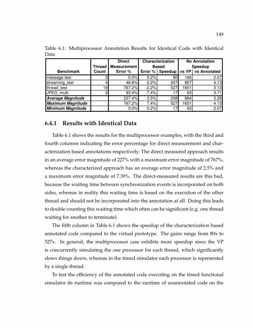
149
Table 6.1: Multiprocessor Annotation Results for Identical Code with IdenticalData
Thread
Direct
MeasurementBenchmark Count Error % Error % Speedup vs VP vs Annotated
message test 3 0.0% 0.2% 80 166 2.07
streaming_test 4 48.8% 0.2% 207 857 4.13
thread_test 19 767.2% -2.2% 527 1651 3.13
JPEG_multi 5 93.4% -7.4% 17 63 3.71
Average Magnitude 227.4% 2.5% 208 684 3.26
Maximum Magnitude 767.2% 7.4% 527 1651 4.13
Minimum Magnitude 0.0% 0.2% 17 63 2.07
Characterization
Based
No Annotation
Speedup
6.4.1 Results with Identical Data
Table 6.1 shows the results for the multiprocessor examples, with the third and
fourth columns indicating the error percentage for direct measurement and char-
acterization based annotations respectively. The direct measured approach results
in an average error magnitude of 227% with a maximum error magnitude of 767%,
whereas the characterized approach has an average error magnitude of 2.5% and
a maximum error magnitude of 7.39%. The direct-measured results are this bad,
because the waiting time between synchronization events is incorporated on both
sides, whereas in reality this waiting time is based on the execution of the other
thread and should not be incorporated into the annotation at all. Doing this leads
to double counting this waiting time which often can be significant (e.g. one thread
waiting for another to terminate).
The fifth column in Table 6.1 shows the speedup of the characterization based
annotated code compared to the virtual prototype. The gains range from 80x to
527x. In general, the multiprocessor case exhibits more speedup since the VP
is concurrently simulating the one processor for each thread, which significantly
slows things down, whereas in the timed simulator each processor is represented
by a single thread.
To test the efficiency of the annotated code executing on the timed functional
simulator its runtime was compared to the runtime of unannotated code on the

150
same simulator. The sixth and seventh columns in Table 6.1 show the speedup
of unannotated code running on the functional simulator compared to the virtual
prototype and the annotated code respectively. The slowdown due to the annota-
tions on average was a factor of 3.3x. This slowdown is much less than that of the
uniprocessor tests for MuSIC, because of the large amount of interaction between
threads in these applications, each of which requires a switch to the simulation
manager, whereas the uniprocessor applications have none of these calls.
The annotator was also run on a multi-threaded JPEG encoder ported from
PThreads, featuring five threads. It was evaluated on images of the following sizes:
32 x 32, 64 x 64, and 160 x 160. For these cases the error was below 8.2%, and the
speedup was between 14x and 18x. The speedup is not that great because the
source code here is very low level, and so the annotations are at a very fine level
of granularity. This causes many context switches between the threads and the
SystemC scheduler, which significantly slows things down.
6.4.2 Results with Different Data
The results so far mentioned are so accurate in part because they are annotat-
ing the same control flow graph with performance measured from the application
running on the same data. To better evaluate the performance it is necessary to
compare the accuracy of the annotated code running on different data and differ-
ent control flows than those used in the characterization. This section presents
the results for the tests that were easily modified to have different execution flows
either by changing constants or running them on different input files.
First, the multiprocessor JPEG encoder was trained and tested on different sizes
of images, and its accuracy wasn’t significantly impacted with its error staying
within 8.2%. We then ran the streaming test multiprocessor benchmark on stream
files with 15, 20, 40, 100, and 500 elements. We then measured the accuracy of each
of the generated annotated source files for each number of elements running on all
of number of elements. The results had 0.7% maximum error magnitude, and an

151
1.000
1.200
1.400
1.600
1.800
2.000
2.200
2.400
2.600
2.800
3.000
1 3 5 7 9
Number of Worker Threads
No
rm
ali
zed
Valu
e
Normalized VP
Execution Time
Normalized Char. Based
Execution Time
Normalized Annotation
Time
Figure 6.11: Normalized execution and annotation times for streaming test withvarying numbers of worker threads

152
average error magnitude of 0.3%.
Finally, the number of worker threads in streaming test were then varied from 1
to 10 for a file with 500 elements. These had a maximum error magnitude of 0.26%
when running on the same data. Figure 6.11 shows the normalized execution and
annotation times for the initial runs- this shows that the annotated code scales
significantly better than the VP. All of the generated source files were then tested
on all of the worker thread configurations, and had a maximum error magnitude
3.03%. The speedup for the one worker was 46x.
6.4.3 Analysis
So far, for applications that do not directly access architecture addresses, our
annotation accuracy is within 5% for both uni-processor and multi-processor ap-
plications running on the same data sets. For different data, only the dhrystone
benchmark had significantly reduced accuracy. The other benchmarks examined
were either operating on data from files or doing multiprocessor communication,
neither of which has significant cache activity. The generally excellent accuracy is
misleading. This work only annotated measured timing results from the virtual
prototype, and the tests run so far are fairly simple and with very regular memory
access patterns. Thus most of the programs fit into the instruction cache, and there
is little contention for the shared memory. For more complicated examples that are
impacted by contention in the communication system or caching effects, we expect
the accuracy to decrease.
The speed of the annotated code has been good, especially for multiprocessor
benchmarks. While measuring cycles-per-second of an event based simulator is
not fully fair, it does show how our simulation performs compared to the virtual
prototype. The range of speedup was between two and four orders of magnitude.
It is important to note that little effort has been made to optimize the speed of
the functional simulator. In addition to speeding up the code, performance can be
increased by combining annotations in straight line application code and also by

153
experimenting with different compilation options. Finally, switching to a commer-
cial SystemC simulator may further increase the annotation performance.
6.5 Discussion
This chapter presented extensions to the uniprocessor annotation technique so
that it was scalably extended to multiprocessor annotation while maintaining good
accuracy. This is done by special handling of startup delays and interprocessor
communication function delays. The next chapter presents the annotation results,
and shows that the characterization-based approach achieves good accuracy.
6.5.1 Limitations
6.5.1.1 Framework Limitations
This framework is implemented as a proof of concept and does have some lim-
itations. Most of these limitations could be overcome with more work, and they
do not impact the results obtained from the framework.
Currently the framework does not fully parse the original C application code. It
makes some assumptions on the syntax, such as requiring curly braces for all loop
and if-then-else clauses. Furthermore, its accuracy can be impacted by putting
multiple commands on the same line, and this is something that debuggers can
have problems with. These issues could be resolved by doing a more complete
parsing of the source files, staying within the syntax limitations, or by using a
code reformatter such as Uncrustify[15].
Also, because the framework does not parse the original application code an-
notations can be placed in illegal places. This is generally solved by manually relo-
cating offending annotations. For the MuSIC functional simulator the Sometimes
annotations are placed before variable declarations, for the MuSIC functional sim-
ulator this is a problem because the annotated code is compiled with Visual C++

154
2005 as C-code, which does not allow function calls before variable declarations.
It is important to note that the XScale annotated applications do not suffer this
limitation since they are compiled by GCC, and after minor modifications to the
annotation code4 none of the annotated applications needed to be modified man-
ually in order to compile and execute properly after annotation.
All of the experiments are run on target applications compiled with out opti-
mization. Using compiler optimizations makes obtaining the accurate annotations
more difficult. This also impacts debuggers, and work such as [150] addresses
it. The annotation only operates on execution times of instructions, so it does not
need to deal with values like a debugger would.
6.5.1.2 Simulator Limitations
The functional simulator for MuSIC does have a few limitations. First, it is only
for the control processors and it does not model the SIMD elements or any of the
accelerators. Also, it does not execute properly on architecture-specific addresses.
It is possible to re-map constants in the original application code to appropriate
constructs in the simulator, but it cannot handle applications that directly refer to
those addresses.
4The block handling was slightly different due to how the debug information was annotated.Also blocks needed to be sliced at the exit and entry points.

155
Chapter 7
Conclusions
This is an exciting and challenging time in the field of embedded systems de-
sign. The continuation of Moore’s Law has enabled an unprecedented amount of
computational capability to be integrated onto a single microchip. This has led to
heterogeneous systems that are highly concurrent and have a growing number of
software programmable elements. To cope with this increasing complexity, the use
of high level models for design space exploration and early software development
has become critical. While cycle-level simulation technologies have made great
strides in the past decade, they still may be overwhelmed by large concurrent sys-
tems, and they are difficult to create and modify. We contend that it is important
to use multiple levels of abstraction and that these are most effective if there is a
way to propagate performance data from lower-level models up to higher-level
models.
This thesis has attacked the problem of modeling microprocessor performance
in embedded systems at different levels of abstraction, and through annotating
timing information from cycle-level models back to the original application source
code. After motivating the problem, we reviewed system level design with specific
emphasis on the different levels of simulating microprocessor performance in the
design process. We then presented an intuitive and highly retargetable approach

156
for modeling a processor’s microarchitecture using Kahn Process Networks. This
was followed by a high-level model of a multiprocessor where architectural el-
ements are treated as timed resources. Finally, a source-level timing annotation
framework for single and multiprocessor systems was developed. Using this anno-
tation framework, results from slow cycle-level simulations were propagated back
to the original application where they were simulated one to three orders of magni-
tude faster without the underlying architecture, while maintaining good accuracy.
An important result of this timing annotation was the extension of it from unipro-
cessor to multiprocessor by handling each processor’s annotation separately and
then substituting in characterized delays for inter-processor communication func-
tions, which was found to be accurate and made the annotator’s runtime linear in
the sum of the size of the instruction traces.
7.1 Future Work
Our work has explored multiple levels of abstraction for processor modeling,
and also relating one to another via timing annotation. There is much future re-
search possible in this area. We overview it in terms of modeling and annotation.
7.1.1 Modeling
There are many potential extensions for our uniprocessor microarchitectural
models. First and foremost the speed of the uniprocessor models should be im-
proved; potential optimizations include: static scheduling, replacing channels with
global variables, and by reducing the overhead of instruction decoding through
caching decoded instructions or pre-decoding instruction traces. Interesting exten-
sions of these models include modeling more complicated resources (e.g. shared
resources and unpipelined/partially pipelined execution units), superscalar exe-
157
cution1, and expanding the ease of porting and configuring such models (In [110]
we presented a language for quickly describing instruction sets and synthesizing
instruction decoders from them). Our queue based models should port quite nicely
to hardware and could be useful for performance modeling using FPGAs (Field
Programmable Gate Arrays), like in the RAMP project [23].
There are also many interesting directions to go with the multiprocessor mod-
els. One is to expand to more complicated timing models (e.g. pipelining) and
finer grained interfaces while still supporting high-level mapping. Also, it is cru-
cial to be able to easily interface with application models and also with lower-level
simulators (e.g. like a single processor cycle-level simulator). On the application
front our annotation work is a step towards this, and on the architectural front our
ongoing development of MetroII [57] will ease interfacing with other models.
7.1.2 Annotation
There are many interesting extensions and applications of our performance
backwards annotation work. Here we list a couple promising paths going forward.
7.1.2.1 Performance Optimizations
Currently, there is huge potential for improving the runtime of the annotation
framework and the speed of the generated annotated code. Right now the frame-
work is written in the interpreted language Python. We expect its performance
would substantially improve if it were rewritten in C++. Also, the processing of
execution trace files is a significant portion of the runtime; this could be reduced
by further optimizing the trace file format, or by having the annotation framework
run concurrently with the virtual prototype generating the instruction traces (and
thus not having to save the traces on disk).
1An abstract superscalar extension of our models was created by Qi Zhu and Haibo Zeng as aclass project.
158
The execution speed of generated code can be improved as well. Currently
each line of source code is separately annotated with delays, and there is special
handling of for and while loops. By analyzing the program’s flow, the annotations
of multiple lines that always execute in the same order into a single annotation.
For the multiprocessor case, the execution speed of annotated applications could
improve significantly by having each thread (processor) store its time locally and
only make synchronize timing with the other threads (processors) when a function
call to the operating system causing interprocessor communication occurs.
7.1.2.2 Handling Optimized Code
It would be quite interesting to extend the annotator to operating on optimized
code. As of now it has run on unoptimized executables. This should be possible
by leveraging work on debugging optimized code like that presented in [150].
7.1.2.3 Memory and Communication Annotation
Source-level timing annotation works well in some cases, its accuracy can sig-
nificantly decrease if the given application’s performance depends significantly
upon communication traffic, and especially so if this traffic is irregular or data
dependent. For these cases the communication aspects of the application should
be represented in the annotations and attached to a simplified architectural model
(like the one developed in Chapter 3) so as to enable more accurate analysis during
architectural exploration.
Adding memory and communication to the annotation framework presents
some unique challenges. The first challenge is that of storing memory and com-
munication traffic. If individual addresses are stored for each execution then the
memory usage of the annotator grows incredibly quickly. Annotating memory
traffic amounts instead of actual addresses is one way to handle this, and should
work well for certain classes of applications, like streaming computation. There
is also the challenge of what to annotate for memory and communication traffic.

159
Instruction traffic is straight forward to handle, but accesses to data might vary
wildly based on pointers, array indices, or other dynamic factors. One interesting
approach is to map the host-machine’s addresses to calls in the target model. A
simpler, but less accurate, option is to just annotate the used memory traffic and
possibly annotate it with statistical miss rates.
7.1.2.4 Combining Annotation with Timing Analysis
Another interesting idea is combining annotation with timing analysis tools
such as AbsInt’s worst case timing analysis tools [2]. In particular, the annota-
tion framework could be leveraged to automatically add additional annotations to
analyzed code and increase the applicability of such timing analysis tools. Further-
more, annotated code could be generated from such tools and mixed with back-
wards annotated code and dynamic simulation for system-level exploration.
7.2 Discussion
Figure 7.1 summarizes the future extensions of the modeling and annotation
work. In particular, it highlights attaching the uniprocessor models to the mul-
tiprocessor models and extending the annotator to handle memory and commu-
nication traffic. This extended annotated code could then be attached to abstract
architectural models, such as the ones presented in this dissertation. Below we
highlight other promising future directions to enable productive system-level de-
sign.
Since multiprocessors are becoming prevalent in all aspects of computation
there are many potential gains with them. The application of parallel processing to
multiprocessor embedded system simulation, can potentially greatly increase the
performance of such simulations. Also, since the annotation handles each proces-
sor’s trace independently, it should be easy to parallelize.
Standardization of interfaces and levels of abstraction is of great importance.

160
Cycle-Accurate
Models
Instruction Level
Models
Algorithmic
Models
Logic Gates
Layout
Actual Gates
Register Transfer
Level Models
Transaction-Level
Models
Algorithmic
Models
Extended
Annotation
Framework
Extended
Multiprocessor
Modeling
Uniprocessor
Modeling
Hardware View Software/CPU View
Timed
Instruction
and
Memory
Trace
Timing +
Communication
Annotated
Application
Application
Code and
Binary
Timing
Annotated
Application
Figure 7.1: Future work summarized in terms of levels of abstraction. Dashed linesrepresent extensions and new areas of work. Solid lines represent work presentedin this dissertation.
The emergence of SystemC [8] and its transaction-level modeling libraries [14, 131]
has enabled an ecosystem of transaction-level tools for hardware, but microproces-
sor and software performance modeling remains relatively closed due to a lack of
interface standards. In particular, creating extension interfaces for microprocessor
simulators is of great importance. Without such standards developing, porting and
applying tools, such as the ones developed in this thesis, is unnecessarily compli-
cated. This is not merely an academic concern, for recently IBM and Tensilica have
called for such standards [130]. The UNISIM framework [25] is an academic project
going in this direction with SystemC-based modular multi-level simulator devel-
opment environment with support for the import of external simulators. Also, the
emergence of free fast instruction set simulators from Imperas [48] and Virtutech
(for academic users) [67] provides some key pieces for this sort of research. Projects
such as GEMS [104] from Wisconsin, build upon these technologies to create cycle
level models.

161
From a theoretical perspective there needs to be more work done on defin-
ing different levels of abstraction and their different levels of relationship. Cur-
rently, most transaction level modeling is done either totally untimed or at the
cycle level. Furthermore, the relationships between the different levels of abstrac-
tion for transaction-level modeling are still somewhat unclear and require further
definition. This is especially true from the perspective of different communication
interfaces, protocols, and models of computation. The tagged signal model [96]
and, more recently, Passerone’s work the agent algebra [120] have looked at such
comparisons and interfacings of different models of computation.

162
Bibliography
[1] 802.11 wireless standard (Wikipedia) -
http://en.wikipedia.org/wiki/IEEE 802.11.
[2] AbsInt Website - http://www.absint.com.
[3] Arm website: http://www.arm.com.
[4] FastVeri Product Overview -
http://www.interdesigntech.co.jp/english/fastveri/.
[5] International Technology Roadmap for Semiconductors, 2004.
http://public.itrs.net/.
[6] Mips web site: http://www.mips.com.
[7] Open Core Protocol International Partnership Website:
http://www.ocpip.org.
[8] Open SystemC Initiative Web Site: http://www.systemc.org.
[9] Power architecture website: http://www.power.org.
[10] SDR Forum Website- http://www.sdrforum.org.
[11] SpecC Website: http://www.cecs.uci.edu/∼specc/.
[12] SystemC Verification Library (SVC) available at: http://www.systemc.org.

163
[13] The GNU Profiler -
http://www.gnu.org/software/binutils/manual/gprof-2.9.1/gprof.html.
[14] Transaction Level Modeling using OSCI TLM 2.0.
[15] Uncrustify web site: http://uncrustify.sourceforge.net/.
[16] VaST Website: http://www.vastsystems.com.
[17] W. Eatherton ‘The Push of Network Processing to the Top of the Pyra-
mid,’ keynote address at the Symposium on Architectures for Network-
ing and Communications Systems, October 26-28, 2005. Slides available at:
http://www.cesr.ncsu.edu/ancs/slides/eathertonKeynote.pdf.
[18] Wikipedia (February 2008) Instructions Per Second at:
http://en.wikipedia.org/wiki/Instructions per second .
[19] Cadence Design Systems Inc (1998). Cierto vcc user guide [online] at:
http://www.cadence.com.
[20] John Moondanos Alberto Sangiovanni-Vincentelli Abhijit Davare, Qi Zhu.
JPEG Encoding on the Intel MXP5800: A Platform-Based Design Case Study.
In IEEE 2005 3rd Workshop on Embedded Systems for Real-time Multimedia,
September 2005.
[21] Casey Alford. Virtual prototyping benefits in safety-critical automotive sys-
tems. Whitepaper available at: www.vastsystems.com, October 2005.
[22] Jeff Andrews and Nick Baker. Xbox 360 System Architecture. Micro, IEEE,
26(2):25–37, March-April 2006.
[23] Arvind, Krste Asanovic, Derek Chiou, James C. Hoe, Christoforos
Kozyrakis, Shih-Lien Lu, Mark Oskin, David Patterson, Jan Rabaey, and John
164
Wawrzynek. RAMP: Research Accelerator for Multiple Processors - A Com-
munity Vision for a Shared Experimental Parallel HW/SW Platform. Techni-
cal Report UCB/CSD-05-1412, EECS Department, University of California,
Berkeley, Sep 2005.
[24] Krste Asanovic, Ras Bodik, Bryan Christopher Catanzaro, Joseph James
Gebis, Parry Husbands, Kurt Keutzer, David A. Patterson, William Lester
Plishker, John Shalf, Samuel Webb Williams, and Katherine A. Yelick. The
Landscape of Parallel Computing Research: A View from Berkeley. Tech-
nical Report UCB/EECS-2006-183, EECS Department, University of Califor-
nia, Berkeley, Dec 2006.
[25] David August, Jonathan Chang, Sylvain Girbal, Daniel Gracia-Perez, Gilles
Mouchard, David A. Penry, Olivier Temam, and Neil Vachharajani. Unisim:
An open simulation environment and library for complex architecture de-
sign and collaborative development. Computer Architecture Letters, 6(2):45–
48, February 2007.
[26] Felice Balarin, Massiliano Chiodo, Paolo Giusto, Harry Hsieh, Attila Jurec-
ska, Luciano Lavagno, Claudio Passerone, Alberto Sangovanni-Vincentelli,
Ellen Sentovich, Kei Suzuki, and Bassam Tabbara. Hardware-software co-
design of embedded systems: the Polis approach. Kluwer Academic Publishers,
Boston; Dordrecht, 1997.
[27] Felice Balarin, Yosinori Watanabe, Harry Hsieh, Luciano Lavagno, Claudio
Passerone, and Alberto Sangiovanni-Vincentelli. Metropolis: An Integrated
Electronic System Design Environment. Computer Magazine, pages 45–52,
April 2003.
[28] Jwahar R. Bammi, Edwin Harcourt, Wido Kruijtzer, Luciano Lavagno, and
Mihai T. Lazarescu. Software performance estimation strategies in a system-
level design tool. Proceedings of CODES, pages 82–6, 2000.

165
[29] Gerard Berry. The Foundations of Esterel. Proof, Language and Interaction:
Essays in Honour of Robin Milner, 2000.
[30] G. Bilsen, M. Engels, R. Lauwereins, and J. Peperstraete. Cycle-static
dataflow. Signal Processing, IEEE Transactions on [see also Acoustics, Speech,
and Signal Processing, IEEE Transactions on], 44(2):397–408, Feb 1996.
[31] Hans-Martin Bluethgen, Cyprian Grassmann, Wolfgang Raab, Ulrich Ra-
macher, and Josef Hausner. A programmable baseband platform for
software-defined radio. In Proceedings of SDR FORUM 2004, 2004.
[32] Shekhar Borkar. Thousand core chips: a technology perspective. In DAC ’07:
Proceedings of the 44th annual conference on Design automation, pages 746–749,
New York, NY, USA, 2007. ACM.
[33] Shekhar Borkar. Design challenges of technology scaling. IEEE Micro,
19(4):23–29, Jul-Aug 1999.
[34] Joseph T. Buck and Edward A. Lee. Scheduling dynamic dataflow graphs
with bounded memory using the token flow model. Proceedings of IEEE In-
ternational Conference on Acoustics, Speech, and Signal Processing, May 1993.
[35] Doug Burger and Todd M. Austin. The SimpleScalar Toolset Version 2.0.
Tech Report. 97-1342, Department of Computer Science, University of Wisconsin-
Madison, June 1997.
[36] Paul Burns. Software defined radio for 3G. Arctech House, Inc., Norwoood,
MA.
[37] Lukai Cai and Daniel Gajski. Transaction level modeling: an overview. Pro-
ceedings of CODES, pages 19–24, 2003.

166
[38] Lukai Cai, Andreas Gerstlauer, and Daniel Gajski. Retargetable profiling for
rapid, early system-level design space exploration. In Proceedings of DAC,
pages 281–286, 2004.
[39] Lukai Cai, Shireesh Verma, and Daniel D. Gajski. Comparison of SpecC and
SystemC Languages for System Design. Technical Report CECS-03-11, Cen-
ter for Embedded Computer Systems, University of California, Irvine, May
2003.
[40] Rong Chen. Platform-based Design for Wireless Embedded Systems. PhD thesis,
University of California at Berkeley, December 2005.
[41] Xi Chen, Fang Chen, Harry Hsieh, Felice Balarin, and Yosinori Watanabe.
Formal verification of embedded system designs at multiple levels of ab-
straction. High-Level Design Validation and Test Workshop, 2002. Seventh IEEE
International, pages 125–130, 27-29 Oct. 2002.
[42] Xi Chen, Abhijit Davare, Harry Hsieh, Alberto Sangiovanni-Vincentelli, and
Yosinori Watanabe. Simulation based deadlock analysis for system level de-
signs. In Design Automation Conference, June 2005.
[43] Xi Chen, Harry Hsieh, Felice Balarin, and Yosinori Watanabe. Automatic
trace analysis for logic of constraints. Design Automation Conference, 2003.
Proceedings, pages 460–465, 2-6 June 2003.
[44] Xi Chen, Harry Hsieh, Felice Balarin, and Yosinori Watanabe. Logic of Con-
straints: A Quantitative Performance and Functional Constraint Formalism.
IEEE Transactions on Computer-Aided Design of Integrated Circuits and Systems,
August 2004.
[45] Lawrence T. Clark, Eric J. Hoffman, Jay Miller, Manish Biyani, Yuyun Liao,
Stephen Strazdus, Michael Morrow, Kimberley E. Velarde, and Mark A.

167
Yarch. An embedded 32-b microprocessor core for low-power and high-
performance applications. IEEE Journal of Solid-State Circuits, 36(11):1599–
1608, November 2001.
[46] Bob Cmelik and David Keppel. Shade: a fast instruction-set simulator for
execution profiling. In SIGMETRICS ’94: Proceedings of the 1994 ACM SIG-
METRICS conference on Measurement and modeling of computer systems, pages
128–137, New York, NY, USA, 1994. ACM.
[47] Jason Cong, Yiping Fan, Guoling Han, Wei Jiang, and Zhiru Zhang. Behavior
and Communication Co-Optimization for Systems with Sequential Commu-
nication Media. In Design Automation Conference, July 2006.
[48] Imperas Corporation. Open Virtual Platform Website:
http://www.ovpworld.org.
[49] Intel Corporation. “Intel IXP1200 Network Processor,” Product Datasheet,
December 2001.
[50] Intel Corporation. “Intel IXP2855 Network Processor,” Product Brief, 2005.
[51] Intel Corporation. SA-110 Microprocessor Technical Reference Manual. Santa
Clara, CA, 2000.
[52] Intel Corporation. Intel Xscale Microarchitecture User’s Manual. Santa Clara,
CA, March 2003.
[53] Xilinx Corporation. Microblaze Processor Reference Guide.
[54] Xilinx Corporation. Fast Simplex Link (FSL) Bus (v2.00a), December 2005.
[55] Xilinx Corporation. Virtex-II Pro and Virtex-II Pro X FPGA User Guide,
november 2007.
168
[56] Abhijit Davare. Automated Mapping for Heterogeneous Multiprocessor Embedded
Systems. PhD thesis, University of California at Berkeley, September 2007.
[57] Abhijit Davare, Douglas Densmore, Trevor Meyerowitz, Alessandro Pinto,
Alberto Sangiovanni-Vincentelli, Guang Yang, Haibo Zeng, and Qi Zhu. A
Next-Generation Design Framework for Platform-Based Design. In Confer-
ence on Using Hardware Design and Verification Languages (DVCon), February
2007.
[58] E. A. de Kock, G. Essink, W. J. M. Smits, P. vd Wolf, J.-Y. Brunel, W. M. Krui-
jtzer, P. Lieverse, and K. A. Vissers. Yapi: Application modeling for signal
processing systems. Proceedings of Design Automation Conference, pages 402–
405, 2000.
[59] Douglas Densmore. A Design Flow for the Development, Characterization, and
Refinement of System Level Architectural Services. PhD thesis, University of
California at Berkeley, May 2007.
[60] Douglas Densmore, Adam Donlin, and Alberto Sangiovanni-Vincentelli.
FPGA Architecture Characterization for System Level Performance Analy-
sis. Proceedings of Design, Automation, and Test Europe, March 2006.
[61] Srinivas Devadas, Abhijit Ghosh, and Kurt Keutzer. Logic Synthesis.
McGraw-Hill, 1994.
[62] Adam Donlin. Transaction level modeling: flows and use models. Proceed-
ings of CODES, pages 75–80, 2004.
[63] E.Clarke, O. Grumberg, and D. Long. Verification Tools for Finite State Con-
current Systems. In J.W. de Bakker, W.-P. de Roever, and G. Rozenberg, ed-
itors, A Decade of Concurrency-Reflections and Perspectives, volume 803, pages
124–175, Noordwijkerhout, Netherlands, 1993. Springer-Verlag.

169
[64] Stephen Edwards, Luciano Lavagno, Edward A. Lee, and Alberto
Sangiovanni-Vincentelli. Design of Embedded Systems: Formal Models, Val-
idation, and Synthesis. Proceedings of the IEEE, 85(3):366–390, 1997.
[65] Stephen A. Edwards. The Specification and Execution of Heterogeneous Syn-
chronous Reactive Systems. PhD thesis, University of California at Berkeley,
March 1997.
[66] Eetimes.com. ‘Intel cancels Tejas, moves to dual-core designs’,
http://www.eetimes.com/showArticle.jhtml?articleID=20000251, May 7,
2004.
[67] Jakob Engblom and Mattias Holm. A Fully Virtual Multi-Node 1553 Bus
Computer System. In Data Systems in Aerospace, May 2006.
[68] Hans Frischkorn. ‘Automotive SoftwareThe Silent Revolution’ Keynote Ad-
dress at the Automotive Software Workshop, February 2004.
[69] Cyprian Grassmann, Mathias Richter, and Mirko Sauermann. Mapping the
physical layer of radio standards to multiprocessor architectures. In Proceed-
ings of DATE 2007, 2007.
[70] Michael Gschwind. Chip multiprocessing and the cell broadband engine. In
Proceedings of the 3rd conference on Computing frontiers, pages 1–8, New York,
NY, USA, 2006. ACM.
[71] Michael Gschwind, David Erb, Sid Manning, and Mark Nutter. An open
source environment for cell broadband engine system software. Computer
Magazine, 40(6):37–47, 2007.
[72] Rajesh K. Gupta and Giovanni De Michelli. Hardware-software cosynthesis
for digital systems. IEEE Design and Test of Computers, 1993.
170
[73] Matthew R. Guthaus, Jeffrey S. Ringenberg, Dan Ernst, Todd M. Austin,
Trevor Mudge, and Richard B. Brown. Mibench: A free, commercially repre-
sentative embedded benchmark suite. Proceedings of the 4th IEEE International
Workshop on Workload Characterization, pages 3–14, 2001.
[74] Ashok Halambi, Peter Grun, Vijay Ganesh, Asheesh Khare, Nikil Dutt, and
Alex Nicolau. Expression: A language for architecture exploration through
compiler/simulator retargetability. Proceedings of the European Conference on
Design, Automation and Test (DATE), pages 485–490, March 1999.
[75] N. Halbwachs, P. Caspi, P. Raymond, and D. Pilaud. The synchronous data-
flow programming language LUSTRE. Proceedings of the IEEE, 79(9):1305–
1320, September 1991.
[76] D. Harel, H. Lachover, A. Naamad, A. Pnueli, M. Politi, R. Sherman, and
a. Shtul-Trauring. Statemate: a working environment for the development
of complex reactive systems. In ICSE ’88: Proceedings of the 10th international
conference on Software engineering, pages 396–406, Los Alamitos, CA, USA,
1988. IEEE Computer Society Press.
[77] Jens Harnisch. Personal Communication, September 2005.
[78] Graham R. Hellestrand. The revolution in systems engineering. IEEE Spectr.,
36(9):43–51, 1999.
[79] Jorg Henkel, Thomas Benner, Rolf Ernst, Wei Ye, Nikola Serafimov, and Ger-
not Glawe. Cosyma: a software-oriented approach to hardware/software
codesign. Journal of Computer Software Engineering, 2(3):293–314, 1994.
[80] Thomas A. Henzinger, Benjamin Horowitz, and Christoph Meyer Kirsch.
Embedded control systems development with giotto. In LCTES/OM, pages
64–72, 2001.

171
[81] C. A. R. Hoare. Communicating sequential processes. Communications of the
ACM, 21(8):666–677, 1978.
[82] James C. Hoe and Arvind. Synthesis of operation-centric hardware descrip-
tions. Proceedings of International Conference on Computer-Aided Design, pages
511–518, 2000.
[83] Christopher Hylands, Edward Lee, Jie Liu, Xiaojun Liu, Stephen Neuendorf-
fer, Yuhong Xiong, and Haiyang Zheng Yang Zhao. Overview of the ptolemy
project. In Technical Memorandum UCB/ERL M03/25, University of California,
Berkeley, CA 94720, July 2006.
[84] Mentor Graphics Inc. Seamless Product Sheet available at:
https://www.mentor.com/seamless.
[85] SPARC International Inc. The SPARC Architecture Manual, Version 9. Prentice
Hall, Englewood Cliffs, NJ, 2000.
[86] iSuppli Corporation. ‘iSuppli Teardown Reveals Apples iPod
touch is More Than an iPhone Without a Phone’, Available at:
http://www.isuppli.com/news/default.asp?id=8717, December 19 2007.
[87] Gilles Kahn. The semantics of a simple language for parallel programming.
Proceedings of the IFIP Congress, pages 471–5, August 1974.
[88] Shinjiro Kakita, Yosinori Watanabe, Douglas Densmore, Abhijit Davare, and
Alberto Sangiovanni-Vincentelli. Functional Model Exploration for Multi-
media Applications via Algebraic Operators. Proceedings of the Sixth Interna-
tional Conference on Application of Concurrency to System Design (ACSD 2006),
June 2006.
[89] Torsten Kempf, Kingshuk Karuri, Gerd Ascheid Stefan Wallentowitz, Rainer
Leupers, and Heinrich Meyr. A SW performance estimation framework for

172
early System-Level-Design using fine-grained instrumentation. In Proceed-
ings of DATE, 2006.
[90] Kurt Keutzer, Sharad Malik, A. Richard Newton, Jan Rabaey, and Alberto
Sangiovanni-Vincentelli. System Level Design: Orthogonolization of Con-
cerns and Platform-Based Design. IEEE Transactions on Computer-Aided De-
sign of Integrated Circuits and Systems, 19(12), December 2000.
[91] Bart Kienhuis, Ed Deprettere, Kees Vissers, and Peter Van Der Wolf. An
approach for quantitative analysis of application-specific dataflow architec-
tures. Application-Specific Systems, Architectures and Processors, 1997. Proceed-
ings., IEEE International Conference on, pages 338–349, 14-16 Jul 1997.
[92] Bart Kienhuis, Ed F. Deprettere, Pieter van der Wolf, and Kees Vissers. A
methodology to design programmble embedded systems: the y-chart ap-
proach. pages 18–37, 2002.
[93] Tim Kogel, Anssi Haverinen, and James Aldis. OCP TLM for Architectural
Modeling. Whitepaper available at: www.ocpip.org, July 2005.
[94] Edward A. Lee. The Problem With Threads. Technical Report UCB/EECS-
2006-1, EECS Department, University of California, Berkeley, January 2006.
[95] Edward A. Lee and Thomas M. Parks. Dataflow process networks. Proceed-
ings of the IEEE, 83(5):773–801, May 1995.
[96] Edward A. Lee and Alberto L. Sangiovanni-Vincentelli. Comparing models
of computation. In ICCAD, pages 234–241, 1996.
[97] Edward Ashford Lee and David G. Messerschmitt. Static scheduling of syn-
chronous data flow programs for digital signal processing. IEEE Trans. Com-
put., 36(1):24–35, 1987.
173
[98] P. LeGuernic, T. Gautier, M. Le Borgne, and C. Le Maire. Programming real-
time applications with SIGNAL. Proceedings of the IEEE, 79(9):1321–1336, Sep
1991.
[99] Yau-Tsun Steven Li and Sharad Malik. Performance analysis of embedded
software using implicit path enumeration. In Proceedings of Design Automa-
tion Conference, pages 456–461, June 1995.
[100] Yau-Tsun Steven Li, Sharad Malik, and Andrew Wolfe. Effcient microarchi-
tecture modeling and path analysis for real-time software. In Proceedings of
the IEEE Real-Time Systems Symposium, pages 298–307, December 1995.
[101] Yau-Tsun Steven Li, Sharad Malik, and Andrew Wolfe. Performance estima-
tion of embedded software with instruction cache modeling. Proceedings of
the IEEE/ACM International Conference on Computer-Aided Design, pages 380–
387, November 1995.
[102] ARM Ltd. ARM Architecture Reference Manual. Cambridge, England, 2000.
[103] Grant Martin and Andrew Piziali. ESL Design and Verification : A Prescription
for Electronic System-Level Methodology. Morgan Kaufman, San Francisco, CA,
2007.
[104] Milo M. K. Martin, Daniel J. Sorin, Bradford M. Beckmann, Michael R.
Marty, Min Xu, Alaa R. Alameldeen, Kevin E. Moore, Mark D. Hill, and
David A. Wood. Multifacet’s general execution-driven multiprocessor sim-
ulator (GEMS) toolset. SIGARCH Computer Architecture News, 33(4):92–99,
2005.
[105] Carl J. Mauer, Mark D. Hill, and David A. Wood. Full-system timing-first
simulation. In SIGMETRICS ’02: Proceedings of the 2002 ACM SIGMETRICS
international conference on Measurement and modeling of computer systems, pages
108–116, New York, NY, USA, 2002. ACM.

174
[106] Rick Merritt. ‘Multicore puts screws to parallel-programming models’, EE-
Times.com, February 15, 2008.
[107] Trevor Meyerowitz. Metropolis ARM CPU Examples. In Technical Memoran-
dum UCB/ERL M04/39, University of California, Berkeley, CA 94720, September
2004.
[108] Trevor Meyerowitz and Alberto Sangiovanni-Vincentelli. High Level CPU
Microarchitecture Models Using Kahn Process Networks. In Proceedings of
SRC TechCon, October 2005.
[109] Trevor Meyerowitz, Mirko Sauermann, Dominik Langen, and Alberto
Sangiovanni-Vincentelli. Source-Level Timing Annotation and Simulation
for a Heterogeneous Multiprocessor. In to appear in the Proceedings of DATE
2008, March 2008.
[110] Trevor Meyerowitz, Jonathan Sprinkle, and Alberto Sangiovanni-Vincentelli.
A visual language for describing instruction sets and generating decoders. In
Proceedings of OOPSLA Workshop on Domain Specific Modeling, October 2004.
[111] Giovanni De Micheli. Synthesis and Optimization of Digital Circuits. McGraw-
Hill, 1994.
[112] Imed Moussa, Thierry Grellier, and Giang Nguyen. Exploring sw perfor-
mance using soc transaction-level modeling. Prooceedings of DATE, 02:20120,
2003.
[113] Shubhendu S. Mukherjee, Steven K. Reinhardt, Babak Falsafi, Mike Litzkow,
Mark D. Hill, David A. Wood, Steven Huss-Lederman, and James R. Larus.
Wisconsin wind tunnel ii: A fast, portable parallel architecture simulator.
IEEE Concurrency, 8(4):12–20, 2000.
[114] Michiaki Muraoka, Noriyoshi Itoh, Rafael K. Morizawa, Hiroyuki Ya-
mashita, and Takao Shinsha. Software execution time back-annotation

175
method for high speed hardware-software co-simulation. In 12th Workshop
on Synthesis and System Integration of Mixed Information Technologies, pages 169
– 175, October 2004.
[115] Tadao Murata. Petri nets: Properties, analysis and applications. Proceedings
of the IEEE, 77(4):541–580, Apr 1989.
[116] Achim Nohl, Gunnar Braun, Oliver Schliebusch, Rainer Leupers, Heinrich
Meyr, and Andreas Hoffmann. A universal technique for fast and flexi-
ble instruction-set architecture simulation. In DAC ’02: Proceedings of the
39th conference on Design Automation, pages 22–27, New York, NY, USA, 2002.
ACM.
[117] Ilia Oussorov, Primrose Mbanefo, and Wolfgang Raab. System-level design
of umts baseband parts with systemc. In Proceedings of DVCON 2004, 2004.
[118] Sudeep Pasricha, Nikil Dutt, and Mohamed Ben-Romdhane. Extending the
transaction level modeling approach for fast communication architecture ex-
ploration. In DAC ’04: Proceedings of the 41st annual conference on Design au-
tomation, pages 113–118, New York, NY, USA, 2004. ACM.
[119] Sudeep Pasricha, Nikil Dutt, and Mohamed Ben-Romdhane. Fast explo-
ration of bus-based on-chip communication architectures. In CODES+ISSS
’04: Proceedings of the international conference on Hardware/Software Codesign
and System Synthesis, pages 242–247, Washington, DC, USA, 2004. IEEE Com-
puter Society.
[120] Roberto Passerone. Semantic Foundations for Heterogeneous Systems. PhD the-
sis, University of California at Berkeley, May 2004.
[121] David Patterson and John Hennessy. Computer Architecture a Quantitative
Approach, 2nd Edition. Morgan Kaufman, San Francisco, CA, 1996.

176
[122] Joann M. Paul, Donald E. Thomas, and Andrew S. Cassidy. High-level mod-
eling and simulation of single-chip programmable heterogeneous multipro-
cessors. ACM Trans. Des. Autom. Electron. Syst., 10(3):431–461, 2005.
[123] Stefan Pees, Andreas Hoffmann, Vojin Zivojnovic, and Heinrich Meyr. LISA
- machine description language for cycle-accurate models of programmable
DSP architectures. Proceedings of the Design Automation Conference, pages 933–
8, 1999.
[124] David A. Penry and David I. August. Optimizations for a simulator con-
struction system supporting reusable components. In DAC ’03: Proceedings
of the 40th conference on Design automation, pages 926–931, New York, NY,
USA, July 2003. ACM.
[125] Wei Qin. Modeling and Description of Embedded Processors for the Development
of Software Tools. PhD thesis, Princeton University, November 2004.
[126] Wei Qin and Sharad Malik. Flexible and formal modeling of microproces-
sors with application to retargetable simulation. Proceedings of the European
Conference on Design, Automation and Test (DATE), pages 556–61, March 2003.
[127] Wolfgang Raab, Hans-Martin Bluethgen, and Ulrich Ramacher. A low-
power memory hierarchy for a fully programmable baseband processor. In
WMPI ’04: Proceedings of the 3rd workshop on Memory performance issues, pages
102–106, New York, NY, USA, 2004. ACM Press.
[128] Steven K. Reinhardt, Mark D. Hill, James R. Larus, Alvin R. Lebeck, James C.
Lewis, and David A. Wood. The wisconsin wind tunnel: virtual prototyping
of parallel computers. SIGMETRICS Perform. Eval. Rev., 21(1):48–60, 1993.
[129] Mehrdad Reshadi and Nikil Dutt. Generic pipelined processor modeling
and high performance cycle-accurate simulation generation. Proceedings of
the European Conference on Design, Automation and Test (DATE), March 2005.

177
[130] EE Times Rick Merritt. ‘IBM calls for modeling standards’, EEtimes.com.
[131] Adam Rose, Stuart Swan, John Pierce, and Jean-Michel Fernandez. Trans-
action Level Modeling in SystemC. Whitepaper available at: www.systemc.org,
2005.
[132] J.A. Rowson. Hardware/software co-simulation. Design Automation, 1994.
31st Conference on, pages 439–440, 6-10 June 1994.
[133] M.N.O. Sadiku and C.M. Akujuobi. Software-defined radio: a brief
overview. Potentials, IEEE, 23(4):14–15, Oct.-Nov. 2004.
[134] Alberto Sangiovanni-Vincentelli. Defining platform-based design. EE De-
sign, March 2002.
[135] Alberto Sangiovanni-Vincentelli. Quo Vadis, SLD? Reasoning About the
Trends and Challenges of System Level Design. Proceedings of the IEEE,
95(3):467–506, March 2007.
[136] Mirko Sauermann. Iltos-the operating system for embedded
multiprocessors-design and implementation. In Proceedings of IESD
2006, 2006.
[137] Eric Schnarr and James R. Larus. Fast out-of-order processor simulation us-
ing memoization. International Conference on Architectural Support for Pro-
gramming Languages and Operating Systems, 33(11):283–294, 1998.
[138] Greg Spirakis. Keynote Address at the EMSOFT: the conference on embedded
software, 2003.
[139] Kei Suzuki and Alberto Sangiovanni-Vincentelli. Efficient software perfor-
mance estimation methods for hardware/software codesign. Proceedings of
the Design Automation Conference, pages 605–610, 1996.

178
[140] The Metropolis Design Team. The metropolis meta model version 0.4. In
Technical Memorandum UCB/ERL M04/38, University of California, Berkeley, CA
94720, September 14, 2004.
[141] Manish Vachharajani, Neil Vachharajani, David A. Penry, Jason Blome, and
David August. Microarchitectural exploration with Liberty. Proceedings of the
35th International Symposium on Microarchitecture, pages 271–282, November
2002.
[142] Sriram Vangali, Jason Howard, Gregory Ruhi, Saurabh Dighe, Howard Wil-
son, James Tschanz, David Finan, Priya Iyer, Arvind Singh, Tiju Jacob,
Shailendra Jain, Sriram Venkataraman, Yatin Hoskote, and Nitin Borkar. An
80-Tile 1.28 TFLOPS Network-on-Chip in 65nm CMOS. Interational Solid-
State Circuits Conference, Digest of Technical Papers., pages 98–9,589, 11-15 Feb.
2007.
[143] Vojin Zivojnovic and Heinrich Meyr. Compiled hw/sw co-simulation. In
DAC ’96: Proceedings of the 33rd annual conference on Design automation, pages
690–695, New York, NY, USA, 1996. ACM.
[144] CoWare Website:. Coware model library ip listing-
http://www.coware.com/pdf/products/modellibrary iplisting.pdf.
[145] Palm website. ‘Palm TX specifications’,
http://www.palm.com/us/products/handhelds/tx/tx specs.html, Febru-
ary 2008.
[146] Reinhold P. Weicker. Understanding variations in dhrystone performance.
Microprocessor Report, pages 16–17, May 1989.
[147] Andreas Wieferink, Rainer Leupers, Gerd Ascheid, Heinrich Meyr, Tom
Michiels, Achim Nohl, and Tim Kogel. Retargetable generation of TLM bus
interfaces for MP-SoC platforms. Proceeding of CODES, pages 249–254, 2005.

179
[148] Reinhard Wilhelm. Why AI + ILP Is Good for WCET, but MC Is Not, Nor
ILP Alone. In VMCAI 2004, volume 2937 of LNCS, pages 309–322, 2004.
[149] Reinhard Wilhelm, Jakob Engblom, Andreas Ermedahl, Niklas Holsti,
Stephan Thesing, David Whalley, Guillem Bernat, Christian Ferdinand,
Reinhold Heckmann, Frank Mueller, Isabelle Puaut, Peter Puschner, Jan
Staschulat, and Per Stenstrm. The Determination of Worst-Case Execution
Times—Overview of the Methods and Survey of Tools. accepted for ACM
Transactions on Embedded Computing Systems (TECS), 2007.
[150] Le-Chun Wu. Interactive Source-Level Debugging of Optimized Code. PhD the-
sis, University of Illinois at Urbana-Champaign, August 1999.
[151] Roland Wunderlich and James Hoe. In-system FPGA prototyping of an Ita-
nium microarchitecture. Proceedings of IEEE International Conference on Com-
puter Design: VLSI in Computers and Processors, pages 288–94, 2004.
[152] Guang Yang, Yosinori Watanabe, Felice Balarin, and Alberto Sangiovanni-
Vincentelli. Separation of Concerns: Overhead in Modeling and Efficient
Simulation Techniques. In Fourth ACM International Conference on Embedded
Software (EMSOFT), September 2004.
[153] Haibo Zeng, Abhijit Davare, Alberto Sangiovanni-Vincentelli, Sampada Son-
alkar, Sri Kanajan, and Claudio Pinello. Design Space Exploration of Auto-
motive Platforms in Metropolis. In Proceedings of Society of Automotive Engi-
neers Congress, April 2006.
[154] Haibo Zeng, Vishal Shah, Douglas Densmore, and Abhijit Davare. Simple
Case Study in Metropolis. In Technical Memorandum UCB/ERL M04/37, Uni-
versity of California, Berkeley, CA 94720, September 14, 2004.