PRIDE User Manual

PRIDE VERSION 2.0

PRIDE - a model for predicting irrigation crop demands

July 2007

PRIDE User Manual

Contents

1. Introduction 11.1 What is PRIDE? 11.2 History of PRIDE Development 11.3 What can PRIDE do? 11.4 What can’t PRIDE do? 11.5 How do I obtain a copy of the PRIDE software? 21.6 How do I use this document? 2

2. Technical reference 32.1 Irrigation culture (crop) 32.2 Climatic factors 42.3 Crop threshold 62.4 Irrigation systems and practices 62.5 Supply system constraints 7

3. The PRIDE sequence of calculations 93.1 Step 1 – The beginning of the irrigation season 93.2 Step 2 – Average rainfall and evaporation 103.3 Step 3 – Demands for each crop type 113.4 Step 4 – Demand reduction in the first two weeks of the season 113.5 Step 5 – Autumn sub-routines 123.6 Step 6 – Accounting for channel efficiency and channel capacity 143.7 Step 7 – Soil drainage factor 153.8 Step 8 – Reduction factor 153.9 Step 9 – Rationing 16

4. Preparation of input data 174.1 Climate file 174.2 Crop factor file 184.3 Crop area file (optional) 194.4 Measured data (optional) 20

5. Using the PRIDE software 215.1 The File Menu 215.1.1 File – Open 215.1.2 File – Save 215.1.3 File – Save As 215.1.4 File – Exit 21

PAGE i

PRIDE User Manual

5.2 The Define Menu 215.2.1 Define - Run Specifications 225.2.2 Define - Hydroclimatic Factors 235.2.3 Define - Crop Areas 255.2.4 Define - Crop Threshold 265.2.5 Define - Channel Efficiency 285.3 The Edit Menu 295.4 The Run Menu 295.5 The View Menu 305.5.1 View – Plot 305.5.2 View – Output File 315.6 The Help Menu 31

6. Model calibration 326.1 Using annual “at the farm gate” measured data 326.2 Using within-season “at the farm gate” measured data 326.3 Using “at the off-take” measured data 326.4 If no measured data is available 336.5 Other issues 33

7. References 34

Appendix A Crop factors 35

Appendix B Changes made to the PRIDE code 37B.1 Changes that will affect program output 37B.2 Changes that have improved usability 39

PAGE ii

PRIDE User Manual

1. Introduction

1.1 What is PRIDE?In order to manage the process of irrigation supply, managers need tools to be able to predict irrigation demand. To facilitate this process, the PRIDE (Program for Regional Irrigation Demand Estimation) model was developed. PRIDE estimates irrigation demand by using a combination of climate data, crop culture and knowledge of traditional farming practices.

PRIDE is most commonly used to estimate private diverter and irrigation district water demands for use in REALM (REsource ALlocation Model). REALM is a water supply system simulation package. Any water supply system can be configured in REALM as a network of nodes and carriers representing reservoirs, demand centres, waterways, pipes, etc. System changes (e.g. new operating rules, physical stream modification) can be quickly and easily configured and investigated in REALM.

1.2 History of PRIDE DevelopmentPRIDE was originally developed by HydroTechnology in 1995. Since that time there have been two major upgrades in 1998 and 2007. The most recent upgrade included modifying the source code to remove minor calculation errors, further improvements to the usability of the program and an update of the PRIDE user manual.

1.3 What can PRIDE do?A distinct advantage of using PRIDE over traditional techniques (such as regression analysis using historical data) is the ability to account for system change. Changes in crop type, irrigated area and management options can all be successfully accommodated using the PRIDE system. Another advantage is that PRIDE can be used to produce stationary time series of demand, that is, demand at a set level of development (e.g. at year 2000 level of development). These can be input to REALM models, for the development of model scenarios. PRIDE predicts crop water requirements that are independent of changes to restriction policies (i.e. low seasonal allocations) - the correct format for input to REALM.

1.4 What can’t PRIDE do?PRIDE software and input files (e.g. crop factors) have been developed and tested in Victoria for Victorian farming districts. The PRIDE model can be applied (cautiously) to South East Australia, but should not be used to model crop water requirements for locations that differ physically or climatically (e.g. tropical Queensland).

Please note that it remains the user’s responsibility to ensure that PRIDE is applied correctly and that the results are reasonable.

PAGE 1

PRIDE User Manual

1.5 How do I obtain a copy of the PRIDE software?The PRIDE software and user manual are the property of DSE and G-MW. The software is distributed by DSE as “freeware” subject to user terms and conditions. For information about licensing and use contact Barry James, Office of Water, Department of Sustainability (Barry.James@dse.vic.gov.au).

1.6 How do I use this document?This report is aimed at both describing the theoretical framework of PRIDE Version 2.0 and the elements of its operation. This report draws on previous PRIDE documentation, for example the PRIDE User Manual produced by HydroTechnology (1995), on behalf of Goulburn-Murray Water.

Chapter 2 includes background information on the assumptions on which the PRIDE software is based. Chapter 3 steps through the algorithms used by PRIDE to calculate crop water requirements and irrigation demands. Chapter 4 provides advice for the preparation of input files. Chapter 5 is a guide to using the PRIDE software. Chapter 6 is a guide to calibrating model outputs. Additional technical information is provided in the Appendices.

PAGE 2

PRIDE User Manual

2. Technical referenceThe primary purpose of irrigation is to reduce water deficit stress by replenishing soil water at regular intervals. It follows that irrigation water demand will be governed by those factors which determine crop water use - principally the irrigation culture, climate, the characteristics of the soil and the type of irrigation system. However, the farmer's judgement of crop water requirement, based on appearance of the crop and experience, may be as important in determining irrigation water demand as the physical factors. A close relationship exists between the perceived and the actual crop water requirement.

This section presents a discussion of the principal factors affecting irrigation demand including crop culture, climatic influences, soil types, irrigation practices and supply system constraints.

2.1 Irrigation culture (crop)The rate at which water is depleted from the soil will depend on evaporation from the soil surface and transpiration from the crop. The term evapotranspiration is used to describe the sum of soil evaporation and transpiration. To estimate crop evapotranspiration, the water use of a reference crop is used and crop coefficients (Kc) are applied to relate the evapotranspiration of a particular crop (ETc) to that of the reference crop (ET0).

Crop Coefficient (Kc) = Equation 1

The following definitions are provided in Malano (1999:19):

Reference crop evapotranspiration ‘is the potential Et for a specific crop (usually grass or lucerne) and is defined as the Et from an extensive surface of 8 to 15 cm tall, green grass cover of uniform height, actively growing, completely shading the ground and not short of water’.

The crop coefficient (Kc) for a particular crop ‘is determined experimentally and reflects the physiology of the crop, the degree of crop cover, the location and method to compute ET0’.

For an annual crop it is normal to recognise four stages of crop growth: initial, crop development mid season and late season (Figure 1). For a perennial crop there will also be seasonal changes in crop coefficient according to leaf growth and senescence (deciduous crops), or due to changes in the physiological restriction to water flow within the tree (e.g. citrus).

PAGE 3

PRIDE User Manual

Time (days)

Start of water use

End of water use

Stage 1:

Initial

Stage 2:

Crop

Developm

ent

Stage 3:

Midseason

Stage 4:

Late Season

Crop C

oefficient, Kc

Figure 1 Seasonal variation of the crop coefficient, Kc. (Source: Dorrenbos and Pruitt, 1977 in Malano, 1999)

The crop coefficient is dependent on the technique used to calculate ET0. There are a number of methods that can be used to calculate ET0. While it is possible to use a lysimeter to measure ET0 directly, it is more usual to use standard meteorological techniques as an indicative measure of ET0. The most appropriate method will largely be dependent on the available data and that used by modelling packages.

2.2 Climatic factorsPenman-Monteith EquationThe Penman-Monteith equation is the preferred method for calculating ET0 in Allen et al (1998). The Penman-Monteith equation is based on physical relationships and is the preferred method if all the meteorological data is available. The equation requires the following data: Air temperature – maximum & minimum; Wind speed; Relative humidity – maximum & minimum (if not available, vapour pressure can be estimated

using the minimum temperature, by assuming that the minimum temperature equals the dewpoint temperature); and

Number of sunshine hours.

Also, elevation above sea level (to calculate atmospheric pressure) and latitude is required to calculate components of the overall equation. The equation is set out in Chapter 4 (p.65) of Allen et al (1998). Crop coefficients presented in FAO Irrigation and Drainage Paper 56 (Allen et al, 1998) are based on the Penman-Monteith equation.

PAGE 4

PRIDE User Manual

Pan EvaporationAs outlined above, the Penman-Monteith equation requires considerable data that may not be available. Pan evaporation is often available however, and crop reference evapotranspiration can be estimated using this data combined with an empirical pan coefficient:

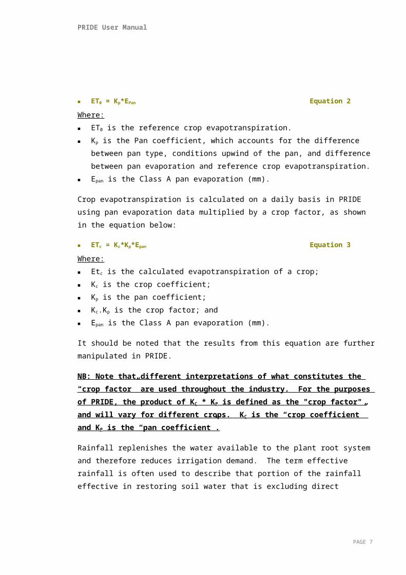
ET0 = Kp*EPan Equation 2

Where: ET0 is the reference crop evapotranspiration. Kp is the Pan coefficient, which accounts for the difference between pan type, conditions

upwind of the pan, and difference between pan evaporation and reference crop evapotranspiration.

Epan is the Class A pan evaporation (mm).

Crop evapotranspiration is calculated on a daily basis in PRIDE using pan evaporation data multiplied by a crop factor, as shown in the equation below:

ETc = Kc*Kp*Epan Equation 3

Where: Etc is the calculated evapotranspiration of a crop; Kc is the crop coefficient; Kp is the pan coefficient; Kc.Kp is the crop factor; and Epan is the Class A pan evaporation (mm).

It should be noted that the results from this equation are further manipulated in PRIDE.

NB: Note that different interpretations of what constitutes the “crop factor” are used throughout the industry. For the purposes of PRIDE, the product of KC * KP is defined as the "crop factor" and will vary for different crops. KC is the “crop coefficient” and KP is the “pan coefficient”.

Rainfall replenishes the water available to the plant root system and therefore reduces irrigation demand. The term effective rainfall is often used to describe that portion of the rainfall effective in restoring soil water that is excluding direct evaporation from the plant canopy, surface run-off and deep percolation below the plant root zone.

Daily time-series of evaporation and rainfall are used as input to the PRIDE model. Evaporation and rainfall are used in every in-season time-step of the model run, to calculate the trigger date for the start of irrigation, and to calculate the crop water requirement that is not satisfied by natural rainfall.

PAGE 5

PRIDE User Manual

2.3 Crop thresholdThe soil moisture “Crop Threshold” value (or MAD value - maximum allowable depletion), the infiltration characteristics of the soil and the drainage status may impact upon irrigation water demand. MAD values are assigned by the PRIDE user for each crop type. Irrigation at the beginning of the season is triggered when the threshold is exceeded. The MAD is determined by the depth of the plant root system and the readily available water. The MAD usually determines when irrigation water needs to be applied to maintain vigorous plant growth. However, where the amount of water entering the soil is limited by poor infiltration, the actual water entry may become a more important factor in determining irrigation frequency.

2.4 Irrigation systems and practicesWhile it is possible to estimate the theoretical crop water requirement, the irrigation demand at the farm gate will always be greater because of the inherent inefficiency in the application of water. The two main factors affecting irrigation efficiency are irrigation distribution systems and irrigation practices.

Inefficiency in water application may occur through spray drift loss, evaporation from the water ponded on the crop foliage or soil surface, surface drainage or deep percolation below the plant root zone and seepage from farm channels, drains and re-use storages. Spray drift loss is a factor in irrigation with overhead sprinklers, particularly for high wind conditions. Surface water run-off is a characteristic of flood irrigation systems. While it is possible in theory to manage irrigation to eliminate run-off, in practice some irrigation water will run-off. Farm development to collect and re-use surface water run-off can reduce irrigation demand on the system.

Deep percolation of irrigation water below the plant roots is an essential requirement of irrigated agriculture, to provide adequate leaching of salt. However, poor uniformity in irrigation often results in deep percolation well in excess of the leaching requirement. The deep percolation will depend on the type of irrigation system and the drainage characteristics of the soil type.

Traditional practices and management factors may also influence water demand. For districts with large areas of annual pasture, water demand at the start of season in autumn is primarily related to traditional practice, and crop water use is a secondary factor in determining water demand.

In the PRIDE model, there is a special sub-routine to simulate the Autumn watering of annual pasture (see Section 3.5). Notionally, the soil drainage factor could be used to indicate inefficiencies within the farm system such as different levels of farm re-use (see Section 3.7).

PAGE 6

PRIDE User Manual

2.5 Supply system constraintsPrivate diverters: Private diverters have licences to divert from a river or creek. In some cases they are part of an unregulated river system and so have to rely on run of river instead of stored water. There are a number of different types of private diverter (PD) licences, including direct irrigation, on-stream winterfill, off-stream winterfill, domestic and stock, dairy, commercial and industrial and non-consumptive use (such as hydro generation). Direct irrigators extract water from the stream/channel at the time the crop or pasture requires it. The volume of water extracted is thus dependant on the type of crop, the area of crop being irrigated, the climate and other variables such as the capacity of the soil to hold water. Direct irrigation demands are usually estimated using PRIDE.

District Irrigators: District irrigators take water from a pipeline or channel system that supplies many diverters. This district supply may be taken from a river or storage. District irrigators may be subject to capacity constraints and distribution losses.

One of the major factors affecting irrigation demand is the availability of supply. The constraints on availability of supply may be divided into those that are related to the available water, and those related to distribution system capacity. When dry conditions prevail and storages are in a healthy state, supply limitations in Victorian irrigation districts are often due to the distribution system itself.

In designing the size of channels and regulating structures, the criterion originally adopted was to allow for the supply of total annual water right in a period of 100 days (HydroTechnology, 1995). This criterion is adequate if irrigation water is to be supplied evenly throughout the season. However, peak demand for water at certain times of the year may be far in excess of the average demand. This is particularly the case in autumn when farmers irrigate annual pastures and in December and January for districts with large areas of perennial pasture. Increasingly this is becoming an issue in mid-summer as irrigated culture has changed from pasture to summer crops.

Capacity constraints can occur anywhere along the system from the major supply routes and channels to the minor infrastructure in the irrigation district. In these peak periods irrigation water supply is rationed and customers are advised of their ration entitlement. Typically this is 10% of annual water right in 10 days (HydroTechnology, 1995), consistent with the design criterion of the system.

Availability of supply from headworks over a particular season can also have a major impact on demand. In Victoria, announcements of seasonal allocations are made early in the irrigation season to allow farmers adequate time to plan crops for the forthcoming year. Allocations at the start of a season are set in accordance with the total volume in store at the time and the expected projected

PAGE 7

PRIDE User Manual

inflow (either recession or 99 percentile) for the remainder of the season. The seasonal allocations are usually adjusted upwards as spring inflows to storage occur but are not adjusted downwards.

A further supply system constraint is the efficiency of the irrigation distribution system. Some flows released from headworks are subjected to substantial losses between the headworks and the district off-take, and within the distribution system.

PAGE 8

PRIDE User Manual

3. The PRIDE sequence of calculationsThe following sequence of calculations is used by the PRIDE model to calculate crop water requirements. These calculations take into consideration plant evapotranspiration requirements, as well as farmer behaviour and soil and infrastructure characteristics.

3.1 Step 1 – The beginning of the irrigation seasonThe PRIDE model is set up to calculate crop water requirements by water year (Jul to Jun) and not by calendar year (Jan – Dec). The model is designed so that irrigation cannot occur before the user defined start date of the irrigation season. Beyond the start date, irrigation begins after the 31st of October or after accounting for the soil moisture over time until a threshold is achieved (whichever comes first).

NB: Default key irrigation season dates are included in Section 5.2.2 (Define - Hydroclimatic Factors).

Threshold values (or MAD values - maximum allowable depletion) are assigned by the user for each crop type. Irrigation is triggered when the threshold is exceeded. In practice, there will be a range of MAD and start times for individual irrigators (HydroTechnology, 1995). However, experience suggests that there is an MAD value which will trigger a general start to the irrigation.

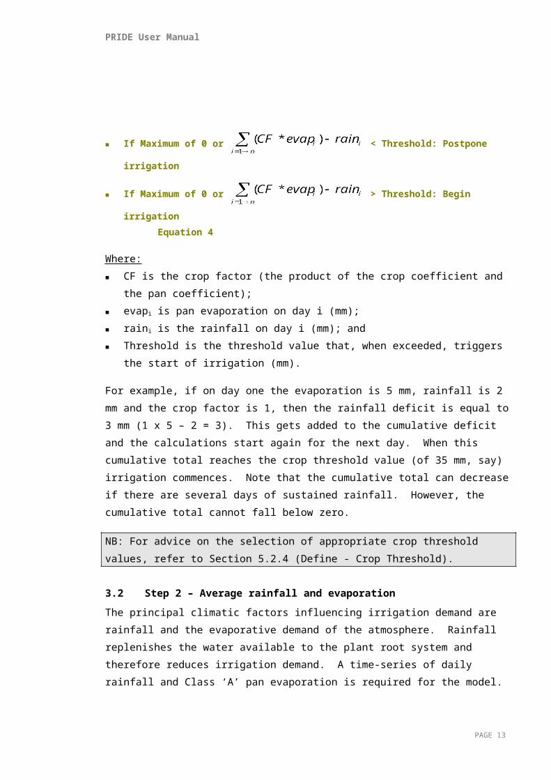
Soil moisture is tracked in the pre-irrigation period by calculating the cumulative rainfall deficit. The cumulative daily rainfall deficit is calculated by:

If Maximum of 0 or < Threshold: Postpone irrigation

If Maximum of 0 or > Threshold: Begin irrigation

Equation 4

Where: CF is the crop factor (the product of the crop coefficient and the pan coefficient); evapi is pan evaporation on day i (mm); raini is the rainfall on day i (mm); and Threshold is the threshold value that, when exceeded, triggers the start of irrigation (mm).

For example, if on day one the evaporation is 5 mm, rainfall is 2 mm and the crop factor is 1, then the rainfall deficit is equal to 3 mm (1 x 5 – 2 = 3). This gets added to the cumulative deficit and the calculations start again for the next day. When this cumulative total reaches the crop threshold

PAGE 9

PRIDE User Manual

value (of 35 mm, say) irrigation commences. Note that the cumulative total can decrease if there are several days of sustained rainfall. However, the cumulative total cannot fall below zero.

NB: For advice on the selection of appropriate crop threshold values, refer to Section 5.2.4 (Define - Crop Threshold).

3.2 Step 2 – Average rainfall and evaporationThe principal climatic factors influencing irrigation demand are rainfall and the evaporative demand of the atmosphere. Rainfall replenishes the water available to the plant root system and therefore reduces irrigation demand. A time-series of daily rainfall and Class ‘A’ pan evaporation is required for the model. Instead of using rainfall from a single station, the user can specify up to three station records and the weighting assigned to each:

Rain = (Factor1*Rain1) + (Factor2*Rain2) + (Factor3*Rain3) Equation 5

Where: Rain is the adopted daily rainfall (mm); Raini is the daily rainfall at gauge number i (mm); and Factori is the weighting assigned to gauge number i.

Throughout the model, the rainfall and evaporation used is averaged over 14 days. The use of an average rainfall accounts for the fact that irrigation demand will not be based solely on the rainfall for that day, it will also be dependent on the antecedent rainfall. Even if there was no rainfall on a particular day, if the crop water requirement is fulfilled by the average rainfall, then there will be no irrigation demand. The computation of the average rainfall is shown in Equation 6. A similar algorithm is applied to calculate the 14-day average evaporation, as shown in Equation 7.

AvRain = [Rain(i) + Rain(i – 1) + Rain(i-2) +…+ Rain(i-13)]/14 Equation 6

Where: AvRain is the 14-day average rainfall (mm); and Rain is the adopted daily rainfall (mm).

AvEvap = [Evap(i) + Evap(i – 1) + Evap(i-2) +…+ Evap(i-13)]/14 Equation 7

Where: AvEvap is the 14-day average evaporation (mm); and Evap is the adopted daily pan evaporation (mm).

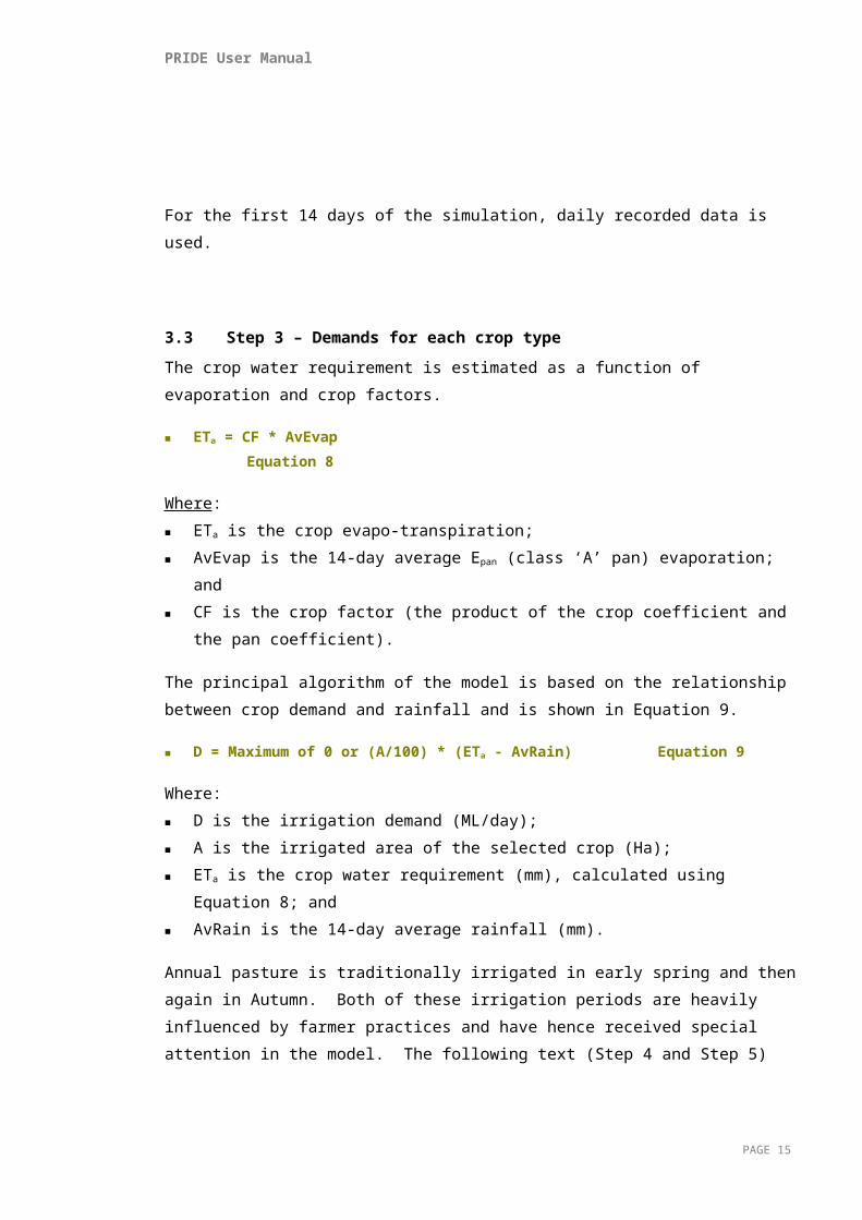
For the first 14 days of the simulation, daily recorded data is used.

PAGE 10

PRIDE User Manual

3.3 Step 3 – Demands for each crop typeThe crop water requirement is estimated as a function of evaporation and crop factors.

ETa = CF * AvEvap Equation 8

Where: ETa is the crop evapo-transpiration; AvEvap is the 14-day average Epan (class ‘A’ pan) evaporation; and CF is the crop factor (the product of the crop coefficient and the pan coefficient).

The principal algorithm of the model is based on the relationship between crop demand and rainfall and is shown in Equation 9.

D = Maximum of 0 or (A/100) * (ETa - AvRain) Equation 9

Where: D is the irrigation demand (ML/day); A is the irrigated area of the selected crop (Ha); ETa is the crop water requirement (mm), calculated using Equation 8; and AvRain is the 14-day average rainfall (mm).

Annual pasture is traditionally irrigated in early spring and then again in Autumn. Both of these irrigation periods are heavily influenced by farmer practices and have hence received special attention in the model. The following text (Step 4 and Step 5) describes the modifications made to account for annual pasture irrigation.

3.4 Step 4 – Demand reduction in the first two weeks of the season

ANNUAL PASTURE ONLYThe annual pasture irrigation demand is reduced in the first two weeks of the irrigation season. In the first week of the irrigation season the demand is reduced by a factor of 0.5. In the second week of the irrigation season the demand is reduced by a factor of 0.25. This occurs in the first two weeks after the start of the season – therefore it won’t be apparent in most seasons unless net evaporation is especially high during the first two weeks and the MAD is exceeded.

PAGE 11

PRIDE User Manual

3.5 Step 5 – Autumn sub-routines

ANNUAL PASTURE ONLYThe autumn irrigation of annual pasture is begun by application of an initial irrigation. Due largely to supply constraints, this volume of water cannot be delivered immediately to all annual pasture irrigators. Instead the ‘starting’ of the annual pasture autumn season is staggered to cope with demand and infrastructure constraints.

PRIDE models the initial autumn watering of annual pasture sub-areas using two different equations. The first equation, Equation 10, is used for that day’s active sub-area, while the second equation, Equation 11, is used for sub-areas that have already received their initial watering. That day’s total demand is equal to the sum of the demand for each sub-area.

DAP = Maximum of 0 or (AAP/100)*SubAreaFraction*(ASMD – AvRain)Equation 10

Where: DAP is the irrigation demand of the active annual pasture sub-area being watered (ML/day); AAP is the total irrigated area of annual pasture (Ha); SubAreaFraction is the percentage of the total annual pasture area represented by that sub-area;

For example, if there are 4 sub-areas then this fraction will be 0.25; ASMD is a user defined parameter representing the Autumn Soil Moisture Deficit (mm); and AvRain is the 14-day average rainfall (mm).

DAP = Maximum of 0 or CFAP*(AvEvap-AvRain)*(AAP/100)*SubAreaFractionEquation 11

Where: DAP is the irrigation demand of the active annual pasture sub-area being watered (ML/day); CFAP is the crop factor for annual pasture (the product of the crop coefficient and the pan

coefficient). AvRain is the 14-day average rainfall (mm); AvEvap is the 14-day average evaporation (mm); AAP is the total irrigated area of annual pasture (Ha); and SubAreaFraction is the percentage of the total annual pasture area represented by that sub-area.

An example of these calculations is shown below for an annual pasture model with 4 sub-areas.

NB: For advice on the selection of a suitable Autumn Soil Moisture Deficit, and number of Annual pasture subareas, refer to Section 5.2.2 (Define - Hydroclimatic Factors).

PAGE 12

PRIDE User Manual

Table 1 Example calculations for an annual pasture model with 4 sub-areas.

Days after start of autumn 1 2 3 4

Annual Pasture Crop Area (Ha) 100 100 100 100Sub Area Fraction 0.25 0.25 0.25 0.25Autumn Soil Moisture Deficit (mm) 14.3 14.3 14.3 14.3Crop Factor 0.8 0.8 0.8 0.8AvRain (mm) 0 0.1 0.3 0AvEvap (mm) 12 11.8 11.6 11.4

Irrigation Demand Sub-area 1 (ML) 3.58 2.34 2.26 2.12Irrigation Demand Sub-area 2 (ML) 0 3.55 2.26 2.12Irrigation Demand Sub-area 3 (ML) 0 0 3.5 2.12Irrigation Demand Sub-area 4 (ML) 0 0 0 3.58

Total Irrigation Demand (ML) 3.58 5.89 8.02 9.94

Once all of the sub-areas have received their initial watering, the annual pasture irrigation demand is calculated using Equation 8. However, until the user specified end of autumn watering, annual pasture demands are subject to two further adjustments.

Adjustment 1: All throughout autumn (including the period of initial watering), if the previous day’s rainfall was greater than 25mm, then a maximum allowable deficit calculation is undertaken, as for the start of the season. If this cumulative deficit is less than the annual pasture threshold (multiplied by a factor) then annual pasture demands are zero. The factor is calculated as:

Factor = (0.5/(SeasonEnd – AutumnStart))*(Today-AutumnStart) Equation 12

Where: SeasonEnd is the Julian day of the year on which the irrigation season ends; AutumnStart is the Julian day of the year on which autumn watering starts; and Today is the current calculation Julian day of the year.

Adjustment 2: Once the initial watering period has been completed, annual pasture demands calculated using Equation 9 will be adjusted for active rainfall. Active rainfall is calculated using:

ActiveRain = (AvRain*14-10)/14 If(ActiveRain<0): ActiveRain = 0 Equation 13

Where: AvRain is the 14-day average rainfall (mm).

PAGE 13

PRIDE User Manual

The active rainfall is then used in place of the average rainfall to calculate autumn annual pasture demands after the initial watering.

DAP = (AAP/100) * (ETa - ActiveRain) Equation 14

Where: DAP is the Annual Pasture irrigation demand (ML/day); AAP is the total irrigated area of Annual Pasture (Ha); ETa is the crop water requirement (mm), calculated using Equation 8; and ActiveRain is the Active Rainfall calculated using Equation 13 (mm).

3.6 Step 6 – Accounting for channel efficiency and channel capacityAn adjustment can be made in PRIDE to ensure that the demand does not exceed the supply channel capacity. This adjustment is shown in Equation 15.

If(D>Ccapacity): D = Ccapacity Equation 15

Where: D is the irrigation demand (ML/day); and Ccapacity is the channel capacity (ML/day).

The adjustment is not necessary for private diverters, or where PRIDE is being calibrated to farm gate data. This option should be used only if the measured data used to calibrate the model is recorded “at the off-take” and the REALM model in which it will be used does not account for capacity constraints (this is rare).

In addition, the efficiency of the supply channel can be accounted for by dividing by a ratio, as shown in Equation 16.

D = D / Ce Equation 16

Where: D is the irrigation demand (ML/day); and Ce is the channel efficiency ratio (≤ 1.0).

Again, this is not required where PRIDE is being fitted to farm gate data and the efficiencies are represented in the REALM model.

As seepage loss may vary with channel running level, the program allows the channel efficiency ratio (Ce) to be set for up to ten flow conditions. The channel efficiency ratios should be less than one. Hence, by dividing by the ratio, the irrigation demand will increase. That is, PRIDE assumes that you will need to deliver more water than is used due to delivery losses from the supply system.

PAGE 14

PRIDE User Manual

NB: For advice on the selection of a suitable channel capacity, and set of channel efficiency ratios, refer to Section 5.2.5 (Define - Channel Efficiency).

3.7 Step 7 – Soil drainage factorRecorded deliveries to the various irrigation districts investigated showed that different volumes of water per hectare for the same crop type were applied in different areas. This was thought to be due to the different soil drainage characteristics and accession to groundwater. A soil drainage factor was introduced to account for this and is shown in Equation 17.

D = D *sdf Equation 17

Where: D is the irrigation demand (ML/day); and Sdf is the soil drainage factor.

The soil drainage factor is the key term used to calibrate the PRIDE model.

NB: For advice on selecting a suitable soil drainage factor, refer to Section 5.2.2 (Define - Hydroclimatic Factors).

3.8 Step 8 – Reduction factorA close examination of actual delivery records (in cases where the season ends mid-May) indicated that by mid-April, some farmers begin to become reluctant to water their pasture into winter. This is mainly due to fear of water-logging should further rain occur and to avoid unnecessary labour and costs in irrigating. To simulate this reduction in demand, the user has the opportunity to apply a factor (the demand reduction ratio) to the estimated demand as shown in Equation 18.

The start date of this reduction in demand is also user defined. The factor is applied to the end of the user defined end date of the irrigation season. Thus, if using this function, it is particularly important that the PRIDE model is run over a water year, and not a calendar year. Otherwise the reduction factor could be applied from April through to December.

D = D * drf Equation 18

Where: D is the irrigation demand (ML/day); and drf is the demand reduction factor (≤ 1.0).

NB: For advice on the selection of a suitable demand reduction factor, refer to Section 5.2.2 (Define - Hydroclimatic Factors).

PAGE 15

PRIDE User Manual

3.9 Step 9 – RationingDue to the limited capacity of the supply infrastructure, some irrigation managers apply rationing during peak periods to ensure the equitable distribution of water. Rationing capacities have been introduced into PRIDE to account for this practice. The application of these rationing capacities is illustrated in Equation 19.

If(D > RatDem): D = RatDem Equation 19

Where: D is the irrigation demand (ML/day); and RatDem is the rationed demand (ML/day).

It should be noted that demand rationing differs from the channel capacity as the rationed volume may be less than the channel capacity.

NB: For advice on the selection of a suitable rationed demand, refer to Section 5.2.2 (Define - Hydroclimatic Factors).

PAGE 16

PRIDE User Manual

4. Preparation of input dataBefore running the PRIDE software, it is necessary to prepare several input files. As a minimum, PRIDE requires a climate file and a crop factor file. Optional inputs include measured irrigation deliveries and a crop area data input file. The following instructions are for preparing input data for the newest version of the PRIDE software. Note that earlier versions of the PRIDE software may have differing input requirements.

A similar format is required for each of the inputs files: Each file is read in free format (i.e. the numbers don’t have to be separated in even columns,

there simply needs to be a space between then). Hence, if preparing the input files in excel, save the data as a space delimited (“.prn” type) file.

The dates entered into PRIDE must be sequential. The program checks that sequential dates have been entered and will not allow the user to proceed until the dates are ordered correctly.

The first few lines can be comments, and must begin with a “!”. This symbol must be left aligned. Useful comments include information on the author, date, project name and number, area being modelled, rainfall and evaporation gauge numbers and the source of data.

It is useful to right align data with a constant column width, and to limit the number of decimal places used. PRIDE output files provide data to one decimal place, so input data to one decimal place is sufficient.

File names and file paths should be as short as practical. PRIDE has a 256 character limit on this.

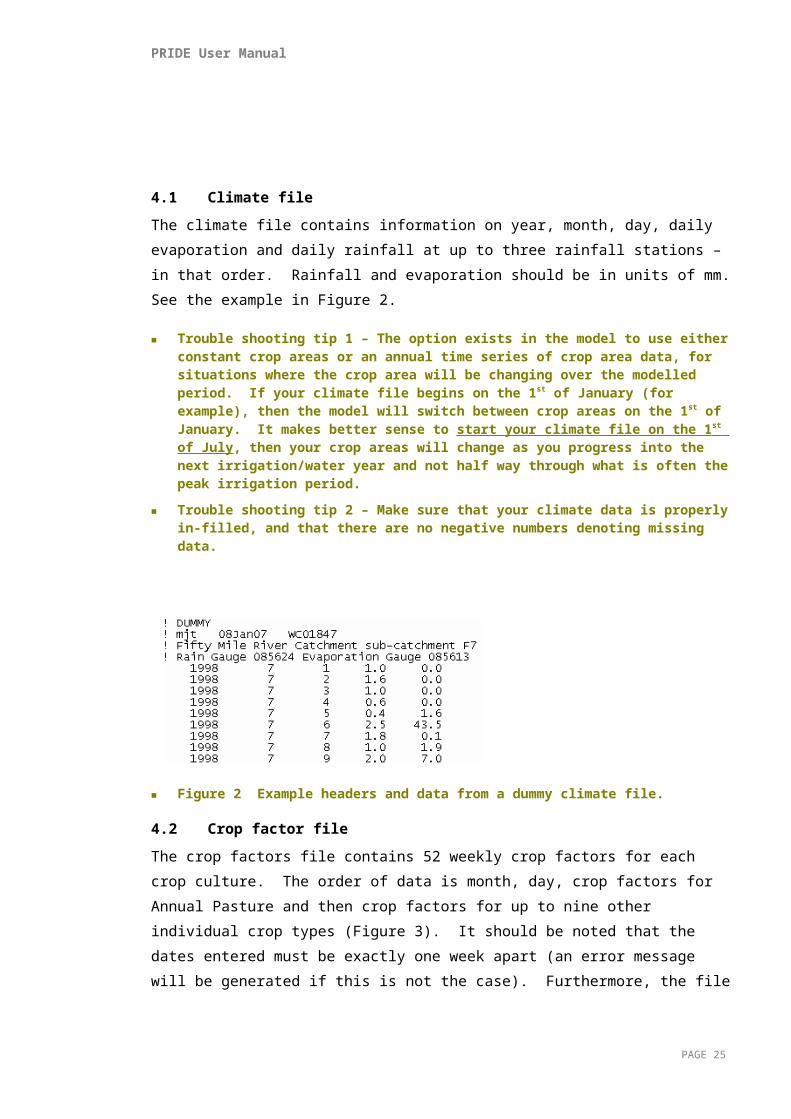
4.1 Climate fileThe climate file contains information on year, month, day, daily evaporation and daily rainfall at up to three rainfall stations – in that order. Rainfall and evaporation should be in units of mm. See the example in Figure 2.

Trouble shooting tip 1 – The option exists in the model to use either constant crop areas or an annual time series of crop area data, for situations where the crop area will be changing over the modelled period. If your climate file begins on the 1st of January (for example), then the model will switch between crop areas on the 1st of January. It makes better sense to start your climate file on the 1 st of July , then your crop areas will change as you progress into the next irrigation/water year and not half way through what is often the peak irrigation period.

Trouble shooting tip 2 – Make sure that your climate data is properly in-filled, and that there are no negative numbers denoting missing data.

PAGE 17

PRIDE User Manual

Figure 2 Example headers and data from a dummy climate file.

4.2 Crop factor fileThe crop factors file contains 52 weekly crop factors for each crop culture. The order of data is month, day, crop factors for Annual Pasture and then crop factors for up to nine other individual crop types (Figure 3). It should be noted that the dates entered must be exactly one week apart (an error message will be generated if this is not the case). Furthermore, the file is structured assuming a non-leap year. The program automatically assigns a crop factor for the extra day in a leap year.

There are generalised crop factors in circulation amongst current PRIDE users. The development of some of these is described in Appendix A. Note that the crop factors currently in use with the PRIDE software have been developed and tested in Victoria for Victorian farming districts. These crop factors can be applied (cautiously) to South East Australia, but should not be used to model crop water requirements for locations that differ physically or climatically (e.g. Queensland).

Figure 3 Example headers and data from a dummy crop factor file.

PAGE 18

PRIDE User Manual

If crop factors for a particular crop do not exist, then guides such as the FAO Guidelines for computing crop water requirements (Allen et al, 1998) and the Manual of Australian Agriculture (Reid, 1990), coupled with local knowledge, can be used to derive appropriate crop factors (remembering that crop coefficients must be multiplied by a pan coefficient!). However, such crop factors will be untested and should be used with caution, particularly if there is no measured data that could be used to calibrate the model.

PRIDE can account for crop rotations, but this requires the external manipulation of crop factors by the user.

Trouble shooting tip 3 - Keep the number and order of crops consistent across all steps of model development.

Trouble shooting tip 4 - PRIDE treats Annual Pasture differently to other crop types, and applies a special subroutine to calculate Annual Pasture water requirements. So that the model knows which data to apply the subroutine to, the model assumes that the first crop is Annual Pasture (e.g. in the crop factor file, time series of crop areas etc.). If you do not wish to model Annual Pasture, then you must put zero Annual Pasture in the crop area file.

Trouble shooting tip 5 – If you are trying to use a crop factor file that has been developed for an older version of the PRIDE software, the sequence of dates may not be accepted by the software. Check that the sequence of dates matches a crop factor file that you know is compatible with the newest version of the PRIDE software.

4.3 Crop area file (optional)The option exists in the model to use either constant crop areas or an annual time series of crop area data, for situations where the crop area will be changing over the modelled period. If using a time series of crop area, the first column of the input file should contain the year (annual or water year, depending on the climate file – see Trouble shooting tip 1). Subsequent columns should contain crop areas in hectares for Annual Pasture and then up to nine additional individual crop types (Figure 4). Keep the number and order of crops consistent across all steps of model development.

Figure 4 Example headers and data from a dummy crop area file.

PAGE 19

PRIDE User Manual

Trouble shooting tip 6 – If your crop areas are small, then your irrigation water requirements will be small also and PRIDE may round the demands to zero. You can multiply crop areas by a factor of ten (for example) in your input file to avoid this, but don’t forget to divide your crop water requirements by ten after running the model.

4.4 Measured data (optional)“Measured data” is measured historic irrigation deliveries on a daily time-step. Two types of data may be available: Data recorded “at the farm gate”. That is, what is used by the farmer to irrigate crops. Data recorded “at the off-take”. That is, the volume of water diverted to an irrigation district.

This data includes delivery losses that occur between the off-take and farm gate.

Historic deliveries are for calibration purposes only, and do not need to be available for the entire simulation period to be included in the model. However, where observed data is not available, a negative value must be entered to indicate that the data is not available (otherwise the model will generate an error message). Historic demands are in ML/day.

PAGE 20

PRIDE User Manual

5. Using the PRIDE software

5.1 The File MenuThe File Menu is for opening existing PRIDE models and saving PRIDE model settings.

5.1.1 File – OpenUse the File>Open command only if you wish to open an existing settings (“.set” type) file. The settings file saves all of the PRIDE run settings and the name of the input and output files. If building a PRIDE model from scratch, then the Define>Run Specification option should be used instead.

5.1.2 File – SaveThis command saves the current settings.

5.1.3 File – Save AsThis command saves the current settings to a new settings (“.set” type) file specified by the user.

5.1.4 File – ExitThe File>Exit command will close the application.

5.2 The Define MenuThe define menu is the most important menu, as this is where the user specifies all the details of the PRIDE model.

PAGE 21

PRIDE User Manual

5.2.1 Define - Run SpecificationsUnder the Define>Run Specifications selection, the user defines the names of all of the input and output files.

A

B

C

D

Part A – Input FilesClimate and crop factor input files should be pre-prepared using the method described in the previous chapter. Output files are created by the PRIDE software, not the user. However, the user should specify the desired name of the output file, including the file directory, for example “D:\PRIDE\example.out”.

Part B – Measured Data“Measured Data” is measured historic irrigation deliveries. Measured Data is an optional input file, as historic deliveries are for plotting purposes only.

Part C – Crop Area DataThe PRIDE software allows the user to specify either constant crop areas (see Section 5.2.3) or an annual time series of crop area data read from an input file, for situations where the crop area will be changing over the modelled period.

Part D – Time stepModel outputs can be either daily crop water demands or daily demands summed by month. The weekly option is not available.

PAGE 22

PRIDE User Manual

Once all of the file selections have been made, the user should press the OK button and proceed to the next menu selection.

Trouble shooting tip 7 – If an error message appears at this point, check to see if you have prepared your input files correctly. Refer to Chapter 4.

Trouble shooting tip 8 – If an error message appears at this point, check to see if you have specified your path names correctly. PRIDE may not have “remembered” the correct path name, particularly if you have not saved your settings or have renamed or switched file folders recently. If PRIDE is not mapping properly, you can copy and paste paths from explorer. It may also be useful to shorten the file path name to something more manageable (<256 characters).

5.2.2 Define - Hydroclimatic Factors Under the Define>Hydroclimatic Factors selection, the user defines a number of parameters and trigger dates.

E

G

F

Part E – GeneralSoil Drainage Factor – The soil drainage factor, otherwise known as the “Soil Factor”, has been introduced into the PRIDE model to account for the fact that recorded deliveries to various irrigation districts (in terms of volumes of water per hectare) differed for the same crop types. This was thought to be due to the different soil drainage characteristics and accession to groundwater. A

PAGE 23

PRIDE User Manual

default value of 1 should be used for the soil drainage factor, unless additional information is available (e.g. measured data to calibrate the model). If the model is calibrated to usage data, then the soil drainage factor should be between 0.8 and 1.2. If it is beyond this value, then another of the inputs (e.g. crop area or recorded usage) could be incorrect. See also Section 3.7 (Step 7 – Soil drainage factor) and Chapter 6 (Model calibration).

Trigger Demand for Rationing - Due to the limited capacity of supply infrastructure, some irrigation managers apply rationing during peak periods to ensure the equitable distribution of water. Rationing capacities have been introduced into PRIDE to account for this practice. If the user does not wish to ration demand, a very large number (e.g. 99999) should be input here. See also Section 3.9 (Step 9 – Rationing).

Demand Reduction Factor - A close examination of actual delivery records indicated that by mid-April, some farmers begin to become reluctant to water their pasture into winter. This is mainly due to fear of water-logging should further rain occur and to avoid unnecessary labour and costs in irrigating. To simulate this reduction in demand, the user has the opportunity to apply a factor (the demand reduction ratio) to the estimated demand. A default factor of 0.5 should be applied, unless additional information is available. If the user does not wish to simulate a reduction in demand then a value of 1.0 should be used. See also Section 3.8 (Step 8 – Reduction factor).

Autumn Soil Moisture Deficit – This parameter refers to Annual Pasture only. A value of 14.3 is commonly used for the Autumn Soil Moisture Deficit factor. See also Section 3.5 (Step 5 – Autumn sub-routines). If the autumn watering irrigation demand spikes unusually (particularly when compared to metered data), the Autumn Soil Moisture Deficit may be set too high.

Annual Pasture Sub-areas – This parameter refers to Annual Pasture only. The autumn irrigation of annual pasture is begun by application of an initial irrigation. Due largely to supply constraints, this volume of water cannot be delivered immediately to all annual pasture irrigators. Instead the ‘starting’ of the annual pasture autumn season is staggered to cope with demand and infrastructure constraints. In PRIDE, this practice is simulated by using annual pasture sub areas. A new sub-area is added daily until all areas are being irrigated. The default number of sub-areas is 6. See also Section 3.5 (Step 5 – Autumn sub-routines).

Part F – RainfallInstead of using rainfall from a single station, the user can specify multiple stations and the weighting assigned to each. Up to three rainfall stations can be specified. The corresponding columns of data must be included in the climate input file. See also Section 4.1 (Climate file). Weightings must add to one.

PAGE 24

PRIDE User Manual

Part G – Time PeriodThe PRIDE model is set up to calculate crop water requirements by water year (Jul to Jun) and not by calendar year (Jan – Dec). The user can specify the start and/or end dates of the irrigation season, autumn irrigation, rationing and reduction in demand. The default values (Table 2) should be used, unless additional information specific to the region, or if measured data that can be used to calibrate the model, is available.

Table 2 Default dates for key periods during the irrigation season.

Time Period Default dates for irrigation districts*

Default dates for private diverters#

Start date of irrigation season 15-Aug 1-Jul

End date of irrigation season 15-May 30-Jun

Start date of autumn irrigation 1-Mar 1-Mar

End date of autumn irrigation 31-May 31-May

Start date of rationing 15-Mar 15-Mar (notional)

End date of rationing 30-Apr 30-Apr (notional)

Beginning of reduction in demand 15-Apr 15-Apr

* Some PDs in the north of Victoria obey irrigation district dates.# Some districts in Victoria, e.g. Werribee, obey PD dates.

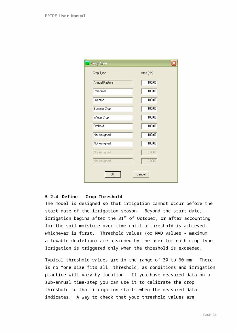
5.2.3 Define - Crop AreasIf an annual time series of crop areas is not used, the user can instead specify a single set of crop areas, which apply to the entire model period. This will produce demands at a constant level of development. Up to ten crops and corresponding areas can be specified, but the first crop must be Annual Pasture. All areas should be in hectares. Keep the order and number of crops consistent across all steps of model development.

Trouble shooting tip 9 – If your crop areas are small, then your irrigation water requirements will be small also and PRIDE may round the demands to zero. You can multiply crop areas by a factor of ten (for example) in your input file to avoid this, but don’t forget to divide your crop water requirements by ten after running the model.

Trouble shooting tip 10 – PRIDE treats Annual Pasture differently to other crop types, and applies a special subroutine to calculate Annual Pasture water requirements. So that the model knows which data to apply the subroutine to, the model assumes that the first crop is Annual Pasture (e.g. in the crop factor file). If you do not wish to model Annual Pasture, then you must enter zero hectares of Annual Pasture as the first crop.

PAGE 25

PRIDE User Manual

Dummy values only

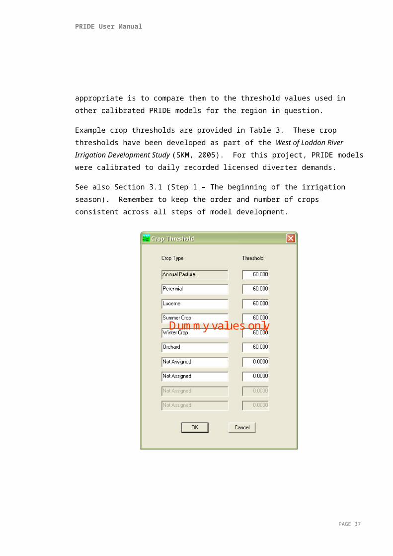
5.2.4 Define - Crop ThresholdThe model is designed so that irrigation cannot occur before the start date of the irrigation season. Beyond the start date, irrigation begins after the 31st of October, or after accounting for the soil moisture over time until a threshold is achieved, whichever is first. Threshold values (or MAD values - maximum allowable depletion) are assigned by the user for each crop type. Irrigation is triggered only when the threshold is exceeded.

Typical threshold values are in the range of 30 to 60 mm. There is no “one size fits all” threshold, as conditions and irrigation practice will vary by location. If you have measured data on a sub-annual time-step you can use it to calibrate the crop threshold so that irrigation starts when the measured data indicates. A way to check that your threshold values are appropriate is to compare them to the threshold values used in other calibrated PRIDE models for the region in question.

Example crop thresholds are provided in Table 3. These crop thresholds have been developed as part of the West of Loddon River Irrigation Development Study (SKM, 2005). For this project, PRIDE models were calibrated to daily recorded licensed diverter demands.

PAGE 26

PRIDE User Manual

See also Section 3.1 (Step 1 – The beginning of the irrigation season). Remember to keep the order and number of crops consistent across all steps of model development.

Dummy values only

Table 3 Example PRIDE crop thresholds for start of irrigation season (SKM, 2005).

Crop type Soil water threshold(mm)

Annual Pasture 38

Perennial Pasture 38

Lucerne 40

Winter Crop 60

Summer crop 38

Orchard 60

Tomatoes 38

Olives 60

Grapes (table and wine) 60

PAGE 27

PRIDE User Manual

5.2.5 Define - Channel EfficiencyUnder the Define>Channel Efficiency selection, the constraining channel capacity (ML) can be specified. In general this function is not used as deliveries are constrained by finite channel capacities in the REALM model. If the capacity is not constraining, the specified channel capacity should be very large (e.g. 99999).

Under the Define>Channel Efficiency selection, the efficiency of the supply channel can also be specified for a range of flows. Again, this function is generally not used. The model assumes that channel efficiency will increase with flow (i.e. demand). Hence efficiency factors must be in ascending order. Values cannot be zero or greater than one.

If using this function, note that an iteration limit has been included in the code. If this iteration limit is triggered during the run time, the user is warned to check the efficiency factors. Note that after this warning has been triggered, no efficiency calculations are undertaken for the remainder of the run. The function used to interpolate between tabulated points is the SPLINE function, from Press et al. (1986).

These options should be used only if the measured data used to calibrate the model is recorded “at the off-take” and the REALM model in which it will be used does not account for channel losses. See also Section 3.6 (Step 6 – Accounting for channel efficiency and channel capacity) and Section 6.3 (Using “at the off-take” measured data).

PAGE 28

PRIDE User Manual

5.3 The Edit MenuUnder the edit menu the user can manually edit the crop factor file (Edit>Crop Factor File), the climate file (Edit>Climate File) or any additional text file (Edit>Any Text File).

5.4 The Run MenuPrior to running the PRIDE model it is recommended that the user select the File>Save or File>Save As option to save the current model settings.

Trouble shooting tip 11 – Have you saved your current settings?

To run the PRIDE model, simply select Run from the menu bar. Alternatively, the black triangular icon can be selected. The model will run automatically.

PAGE 29

PRIDE User Manual

5.5 The View MenuThe View menu is only available when the model has been successfully run.

5.5.1 View – PlotThe View>Plot selection will take the user to a new menu bar and application specifically for plotting output data. There are several options available to the user for scrolling through data plots and for printing plots, either by sending the plot to a printer or by saving the plot as a picture file.

The file menu Page Setup – If sending the plot to a printer, this option allows the user to change the paper

size, page orientation and page margins and to select the preferred printer. Print Plot – Sends the current plot directly to the default/preferred printer. Save plot to file – Allows the user to save the current plot as a Windows Metafile (WMF),

Computer Graphics Metafile (CGM), Bitmap (BMP), PS or HPGL type picture file.

The format menu Selected plots - Allows the user to choose to exclude/include the following plot items:

Crop plot – Up to ten crop types. Measured and total plots – Measured data and total demand. Climate – Rainfall and evaporation.

Grid – Used to switch between grid lines and no grid lines. Legend – Used to switch between a legend and no legend. Plot titles – Allows the user to specify a plot title and labels for the y-axis and x-axis. Zoom – Allows the user to specify the maximum and minimum values on the y-axis and x-

axis. Crop plot options – Allows the user to change the line style, marker style and colour of the

lines representing crop water requirements, measured data and the total crop demand. Climate plot options – Allows the user to change the line style, marker style and colour of the

lines representing rainfall and evaporation.

Previous - Allows the user to scroll backwards through the plot data.

Next - Allows the user to scroll forwards through the plot data.

Close - Closes the plotting application and returns the user to the main program interface.

PAGE 30

PRIDE User Manual

5.5.2 View – Output FileThe View>Output file selection allows the user to look at (but not edit) the PRIDE output file.

5.6 The Help MenuThe Help option provides access to help files. But the help files have been superseded by this document.

PAGE 31

PRIDE User Manual

6. Model calibrationThree types of data may be available to calibrate the PRIDE model: Data recorded “at the farm gate”. That is, what is used by the farmer to irrigate crops. Data recorded “at the off-take”. That is, the volume of water diverted to an irrigation district.

This data does not account for delivery losses. Estimated proportion of licensed volume used, as provided by the rural water authority.

6.1 Using annual “at the farm gate” measured data

(or estimated proportion of licensed volume used)If only annual usage data “at the farm gate” is available, the model can be calibrated by adjusting the soil drainage factor so that the annual total demand is equal to the annual total delivery volume. The relationship between demand and soil drainage factor is linear. So if the calculated demand is too low by 20%, then the user should make the soil drainage factor equal to 1.20.

The soil drainage factor should be between 0.8 and 1.2. If it is beyond this value, then another of the inputs (e.g. crop area or recorded usage) could be incorrect.

Usage data in years of restricted water availability will be below the crop water requirement modelled using PRIDE (i.e. PRIDE will over-predict in restricted years).

If the model will not calibrate, it may be that the input data is in error. A common problem is that crop areas are poorly estimated. In this instance, discuss the limitations of the data with the person who supplied the data. How was the data estimated? Are crop areas in some years more reliable than others? Then concentrate the calibration on the most reliable data, or adjust the crop areas if more reliable information comes to light.

6.2 Using within-season “at the farm gate” measured dataIf within-year (i.e. daily, weekly, monthly etc.) “at the farm gate” data is available, the above advice still applies, but the user has the option to calibrate the model using additional factors in the Define>Hydroclimatic Factors window, e.g. irrigation start date. The crop threshold can also be used to calibrate the model.

6.3 Using “at the off-take” measured dataIf data is available “at the off-take”, the above advice applies. However, the constraining channel capacity (ML) can also be specified and the efficiency of the supply channel can be specified for a range of flows (see Sections 3.6 and 5.2.5). PRIDE is unable to account for changes to irrigation supply infrastructure during the modelled period. Be careful in using these features as normally these effects are allowed for in the REALM model.

PAGE 32

PRIDE User Manual

6.4 If no measured data is availableIf no usage data is available at all, then the user should use the default settings, including a soil drainage factor of 1. If other PRIDE models have been calibrated nearby, the soil drainage factors from these models can be used.

6.5 Other issuesIn the past, some users of PRIDE have had difficulties replicating past model results. If the same input files and parameters are used, the differences could be a result of using different versions of the PRIDE model (the software has undergone several revisions, including a DOS and early Windows version). In the case that model results must be replicated, the user can retrieve the superseded software and PRIDE files from archive. However, the most up-to-date version of PRIDE represents a refined model and should be used preferentially, so it is better to recalibrate the model rather than replicating old results.

PAGE 33

PRIDE User Manual

7. ReferencesAllen, R., L. Pereira, D. Raes, and M. Smith, 1998. Crop evapotranspiration. Guidelines for

computing crop water requirements. Food and Agriculture Organization of the United Nations Irrigation and Drainage Paper 56, Rome.

Doorenbos, J., and W.O. Pruitt, 1984. Crop water requirements. Food and Agriculture Organization of the United Nations Irrigation and Drainage Paper 24, Rome.

DSE and DPI, 2003. Farm Water Use Efficiency Technical Reference Booklet. Department of Sustainability and Environment and Department of Primary Industries, Victoria.

Erlanger, P.D., D.C. Poulton, and P.E. Weinmann, 1992. Development and Application of an Irrigation Demand Model Based on Crop Factors. Conference on Engineering in Agriculture 1992, Albury, Australia. IEAust. Nat. Conf. Publication No. 92/11: 923-298

HydroTechnology, 1995. PRIDE Documentation. Report to Goulburn-Murray Water, May 1995, Report Number MC/44351.010.

Malano, H., 1999. Irrigation and Drainage Management Supplement Study Note. Subject code 421-472, Department of Civil and Environmental Engineering, The University of Melbourne.

Press, W., B. Flannery, S. Teukolsky and W. Vetterling, 1987. Numerical Recipes: The Art of Scientific Computing. Cambridge University Press, Cambridge.

Reid, R. (ed.), 1990. The Manual of Australian Agriculture. The Australian Institute of Agricultural Science, Butterworths, Sydney.

Rendell, R., and D. Thomas, 1985. Water Requirements and Predicted Irrigation Frequencies in the Kerang Region. FDA Internal Report.

SKM, 1998. PRIDE (Draft). Unpublished and uncontrolled user manual for Goulburn-Murray Water. Job number WC00694.

SKM, 2005. West of Loddon River Irrigation Development Study. Final Report. Report for Goulburn-Murray Water. Job number WC01685.

SKM, 2006. Discussion Paper. Report for the West Gippsland Catchment Management Authority. Job number WT01947.

PAGE 34

PRIDE User Manual

Appendix A Crop factorsThe following is an edited excerpt from HydroTechnology (1995). This excerpt has been reproduced to provide information on how crop factors have been developed. But some crop factors may have been superseded:

The crop factors used in PRIDE are shown in Table 4. For computational simplicity the irrigated cultures were restricted to six groups. These were perennial pasture, Lucerne, summer crop, winter crop, orchard and annual pasture.

Table 4 Monthly crop factors used in the PRIDE model (HydroTechnology, 1995)

Jan Feb Mar Apr May Jun1 Jul1 Aug1 Sep Oct Nov Dec

Perennial Pasture & Lucerne

0.80 0.80 0.80 0.80 0 0 0.80 0.80 0.80 0.80 0.80 0.80

Summer Crop 0.88 0.65 0.40 0 0 0 0 0 0 0 0.30 0.80

Winter Crop 0 0 0 0 0 0.20 0.40 0.50 0.70 0.80 0.60 0

Annual Pasture 0 0 0.50 0.80 0 0 0.80 0.80 0.80 0.80 0 0

Orchard 0.79 0.79 0.76 0.60 0 0 0 0 0 0.30 0.53 0.73

(1) Crop factors in the winter period are required to allow determination of the start of the irrigation season.(2) Orchard crop factors subject to review based on further work.

For perennial pasture it was assumed the evapotranspiration is equivalent to a crop factor of 0.8. While some authors have suggested the crop factor for perennial pasture should be lower during December-February, the value of 0.8 has been used in initial development of the model.

Lucerne has a variable crop factor from 0.3 after being cut to 1.0 at flowering. There will also be a seasonal variation in crop factor, depending on whether the Lucerne variety is winter dormant. Recent studies in the Boort District suggest a crop factor of 0.8 for a period prior to the second irrigation after a cut, and 0.95 prior to the third irrigation after a cut. In practice, a crop factor of 0.8 has been used for simplicity.

For summer crop, a November-sown millet crop is used as the basis for estimation of crop factors. Millet accounts for some 60% of summer forage and grain crops in Northern Victoria. The values adopted are those used by Rendell and Thomas (1985).

Trouble shooting tip 12 – If modelling summer vegetables, make sure that you are using the correct crop factors. In the past, “summer crop” crop factors may have been mistakenly used for “summer vegetables”.

For winter crop, a June sown wheat crop is used as the basis for estimating crop factors. Crop factors are adopted from Rendell and Thomas (1985) with the maximum crop factor in October raised from 0.7 to 0.8, consistent with recent field studies (Poulton pers comm).

PAGE 35

PRIDE User Manual

For orchard it is assumed the major crop is stone fruit. Crop factors are taken from Doorenbos and Pruitt (1984) for a dry strong wind and including a ground cover crop. A pan coefficient of 0.8 is assumed in converting the crop coefficient of Doorenbos and Pruitt to an equivalent crop factor.

For annual pasture it is assumed the first irrigation will require 100 mm, and the second irrigation will occur two weeks later and require 50 mm. Subsequent irrigations assume a crop factor of 0.8 (or some other pre-selected factor), i.e. equivalent to reference crop evapotranspiration, except over the period November-January, when no irrigation is assumed.

PAGE 36

PRIDE User Manual

Appendix B Changes made to the PRIDE codeA project was recently undertaken to debug PRIDE, improve the usability of the program and to update the PRIDE user manual. As part of this work, several changes have been made to the PRIDE source code. Some of these changes are designed to remove calculation bugs. The remaining changes are designed to improve the usability of the software.

B.1 Changes that will affect program outputThe completed changes that will affect model outputs are:

1) Previously, PRIDE would always calculate a zero crop water requirement for the 1st of January in leap years. This problem was due to the handling of dates within the program and the structure of the main calculation loop. This caused crop factors to not be properly tracked in leap years. The code has been modified to fix these errors so that a crop water demand is properly calculated on the 1st of January in leap years.

2) In the final day of the season, PRIDE was not applying the Demand Reduction Ratio. This ratio is used to model a reduction in demand that occurs by mid-April, as farmers begin to become reluctant to water their pasture into winter. The code has been fixed so that the Ratio is now applied until the last day of the season, which is specified by the user. Thus, if using this function, it is particularly important that the PRIDE model is run over a water year, and not a calendar year. Otherwise the reduction factor could be applied from April through to December.

3) In previous versions, PRIDE was not applying the efficiency factor correctly.

PRIDE would get into a calculation loop when applying channel efficiency ratios. The model has an algorithm to check that the demand divided by the efficiency factor converges, and if the efficiency factor is too high (i.e. greater than approximately 2) the model will not converge. To fix this, an iteration limit was added to the code. If this iteration limit is triggered during the run time, the user is warned to check the efficiency factors. Note that after this warning has been triggered, no efficiency calculations are undertaken for the remainder of the run.

PRIDE was not applying the correct efficiency factor for a given Demand. The problem was that while interpolating between values in the demand / efficiency table using a “spline” function, the model would re-apply the efficiency value every time an iteration was performed. For example, the user defined channel efficiency ratio may be 0.9, but if it is applied five times then the ratio becomes 0.6 (i.e. 0.9x0.9x0.9x0.9x0.9=0.59049).

The code has also been modified to prevent the user defined efficiency factors from being greater than 1 or less than 0. A check has also been added to ensure that ratios are in ascending order. That is, the model requires that efficiency increases with flow.

PAGE 37

PRIDE User Manual

4) The Annual Pasture irrigation demand was being reduced in the first two weeks of the irrigation season plus one day. The code has been modified so that the demand is only reduced in the first two weeks, as intended.

5) A number of changes were made to the Annual Pasture autumn watering sub-routine:

In times of high rainfall, the Annual Pasture crop water requirement was sometimes a negative number. An extra line of code has been added so that negative demands are reset to zero.

The annual pasture autumn watering sub-routine was designed to finish at the end of autumn, but instead the sub-routine was running to the last day of the season. The code has been modified so that the user can define the end date of autumn watering in the Hydroclimatic Factors window. After the end date, the program reverts back to the standard method for calculating crop water demand. Settings files created in the older versions of the PRIDE software can still be opened in PRIDE. However, the user will be warned that the software has assigned a default date to the end date of autumn watering.

The annual pasture autumn watering sub-routine started on the first day of autumn irrigation plus one. The code has been modified so that the sub-routine begins on the user defined autumn irrigation start date.

It was intended that all through autumn, if the previous day’s rainfall was greater than 25mm, then a maximum allowable deficit calculation should be undertaken, as for the start of the season. However, this calculation was not being executed by the software. Instead, PRIDE would recognise when yesterday’s rainfall was greater than 25mm. On these days the demand was zero. But then the model would revert back to the normal method for calculating the autumn demand. The code has been fixed and the model now tracks the deficit. The formula for calculating the threshold adjustment factor (Equation 12) has also been changed. Previously “Today” was represented by the count day of the simulation. Now “Today” is represented by the Julian day of the current calculation day.

Previously, the formula for calculating Active Rainfall was [(AvRain-10)/14]. Thus, unless the 14-day average rainfall was greater than 10mm, the Active Rainfall would be equal to less than zero, which would be reset to zero. What this means is that typically none of the Annual Pasture crop water requirement would be met by natural rainfall in the autumn season. The Active Rainfall calculation method has been changed, so that Active Rainfall is now equal to [(AvRain*14-10)/14]. It is believed that this was the intended form of the equation.

6) Instead of using rainfall from a single station, the user can specify up to three station records and the weighting assigned to each. However, this function sometimes wouldn’t work when three rainfall stations were specified. The code has been corrected, and the rainfall records are now split appropriately.

PAGE 38

PRIDE User Manual

B.2 Changes that have improved usabilityThe completed changes that will not affect model outputs, but improve the usability of the program, are:

7) In the past, users of the PRIDE software have complained that PRIDE did not properly save model settings. Hence, a prompt to save the current settings has been added to the software. This prompt appears before quitting the program or switching between settings files.

8) Dialog boxes for opening files have been standardised to normal Windows format for ease of use.

9) Users have also found it difficult to enter the file name of input files, as PRIDE will not “remember” what directory it is working in. The software will now “remember” the location of the settings file.

10) Previously the default values and settings within PRIDE were saved to the user’s hard drive. Thus a user could change some of the default parameter values or plot settings. This has now been removed with all default values hard-coded within the program.

11) The PRIDE output is now GetDat compatible –the format of the output is an improvement over the previous version and will facilitate easy import into Excel.

12) The maximum number of days that can be used per simulation has been increased (now 60,000 days, i.e. approximately 164 years).

13) PRIDE treats Annual Pasture differently to other crop types, and applies a special subroutine to calculate Annual Pasture water requirements. So that the model knows which data to apply the subroutine to, it assumes that the first crop is Annual Pasture. Hence the label in the first column of the Define>Crop Area and Define>Crop Threshold windows is now fixed as “Annual Pasture” to avoid misuse.

14) Calculation stability has been improved within the code by denying implicit declaration of variables in most sub-routines.

15) For consistency and appropriateness of nomenclature, the following changes have been made to parameter input names in the Hydroclimatic Factors window:

Was: “Soil deficit factor” Now: “Soil drainage factor”

Was: “Demand rationing factor” Now: “Trigger demand for rationing”

16) Previously, PRIDE would freeze when using the plotting window. This happened when the user clicked the “X” in the top right hand corner of the window. This bug has been fixed so that the user is now returned to the main program.

17) Help -> Licence selection added to the menu and Help -> About selection has been updated.

PAGE 39