Simultaneous Numerical Simulation of the Hydraulic

Fractures Geometry in Multi-Stage Fracturing for

Horizontal Shale Gas Wells. María del Mar Prieto1

1 Chemical Engineering Department, Universidad de los Andes, Bogotá, Colombia.

Abstract

In this study, the hydraulic fracture geometry of multistage treatments is simulated. A simultaneous

numerical simulation strategy is implemented for the three modules that allow for hydraulic

fracture geometry calculation. The implemented modules of the simulation strategy are the fracture

propagation, the formation stress and the flow rate distribution which are coupled to obtain a

simultaneous solution. A second-order partial differential equation that describes the fracture

propagation module is solved using an implicit Finite Difference Method (FDM), taking advantage

of the concept of transmissibility. The flow rate distribution module calculates the inlet flow rate

at each fracture by solving a nonlinear equation system. The formation stress module is described

by a linear equation system, solved with the Discontinuous Displacement Method (DDM) for

induced stress formation calculation. Coupling the modules requires the solution of two implicit

equation systems and the evaluation of a fracture length criterion. A case study based on a single

well (i.e., the X2-HF well) located northeast of the Fuling shale gas field, targeting the Wufeng

and Longmaxi formation. A four-stage stimulation treatment with three fracture clusters is

simulated. The space discretization for each stage is done for 30 elements with 10-time steps of

666 s. The obtained geometry in the mentioned field has a maximum half-length of 165.6 [m] and

a minimum half-length of 136.8 [m]. The numerical solution requires 9.55 s to solve a single-stage

scenario and 34.2 seconds to solve a four-stage scenario.

1. Introduction

In recent years, shale gas production has become the primary source of energy in many countries

(Zhao et al., 2017), which allows the potential increase of reserves. As a result, the development

of these reservoirs has acquired importance in the petroleum industry. Hydrocarbon production of

unconventional reservoirs is a complex task due to the ultra-low permeability and low porosity of

the formations (Lin, Ren, Zhao, & Huang, 2017). These conditions require the implementation of

horizontal well drilling, combined with hydraulic fracturing (Olson & Wu, 2012a). This technique

aims to improve communication channels between the formation and the wells, allowing the

reservoir gas to flow.

Multi-stage hydraulic fracturing is the most common technique for improving

communication channels in unconventional reservoirs. However, this technique is expensive and

generates a high risk of environmental impacts (Lin, Ren, Zhao, & Huang, 2017). The design of

multi-stage hydraulic fracturing treatment has been extensively studied, involving the calculation

of variables such as the fracture length, width, spacing and cluster spacing. These variables

determine the hydraulic fracture geometry and its distribution within the formation.

Knowing the geometry and the distribution of hydraulic fractures, the Stimulated Reservoir

Volume (SRV) can be calculated allowing a better estimation of gas production of the reservoir

(Lin, Ren, Zhao, & Huang, 2017). For this reason, it is essential to estimate the geometry and the

distribution of the hydraulic fractures before the stimulation treatment. With this information, the

designer of the stimulation treatment can predict the adequate geometry for the reservoir, allowing

the determination of the maximum gas production. Since the simulations of these processes are

computationally expensive and demanding (Ren, Lin, & Zhao, 2018), obtaining fast and reliable

results are important for improving the hydraulic fracturing process design in an economically

favorable manner.

Multiple numerical methods have been developed to simulate the hydraulic fracture

geometry and distribution inside the formation. The most relevant works are presented in Table 1,

categorizing them by the year of publication and their contribution to the modelling of the physical

phenomena.

Table 1. Works of simulation of hydraulic fracturing in unconventional reservoirs.

Reference Contribution

Rogers et al., 2010

Developed a framework to integrate natural fracture systems with

hydraulic fractures through a Discrete Fracture Network (DFN) code that

models and predicts growth and propagation of the hydraulic fracture

within a network of existing natural fractures. A hybrid Finite

Element/Discrete Element code was used to validate the results of DFN

hydraulic fracture simulations.

Meyer & Bazan,

2011

Formulated a numerical simulator of an induced hydraulic Discrete

Fracture Network (DFN) to predict their propagation and behavior in

shale and unconventional formations, generating a Stimulated Reservoir

Volume (SRV). The solution methodology involves coupling the mass,

momentum, continuity, and constitutive equations for a pseudo 3D

induced hydraulic fractures system.

Weng et al., 2011

Proposed a complex fracture network model to simulate the propagation,

deformation and fluid flow of the hydraulic fracture in the unconventional

fracture model (UFM). The UFM solves the constitutive equations with

multiple propagation fracture tips and considers the interaction hydraulic-

fracture/natural-fracture by computing the stress-shadow effect on each

fracture by the adjacent fractures using an analytical model.

Olson & Wu,

2012a

Described a non-planar single fracture model to simulate the complex

hydraulic fracture propagation, considering a critical parameter that is the

sequential or simultaneous fluid injection using two different pseudo-3D

element boundaries, displacement discontinuity method, based on

hydraulic fracture simulators. The uncoupled mechanics and fluid flow

equations are simultaneously solved using Newton’s Method and Picard

iteration.

G. Yu & Aguilera,

2012

Developed an analytical 3D model to simulate the growth of stimulated

reservoir volume (SRV) with time. The SRV simulation involves two

steps, including calibration of the model by determining its hydraulic

diffusivity coefficients and predicting the geometry of SRV. The

analytical model is compared with a numerical model that is built based

on the same assumptions for the analytical model.

Huang et al., 2014

Presented two geomechanical sensitivity analyses that quantify variations

in Productive SRV, synthetic MS events and pressure field for upon

stimulation of DFN. The geomechanical model used a pseudo-3D DFN

simulation code, and the stresses induced by fracture deformation were

calculate using the Displacement Discontinuity Method.

Wu & Olson,

2015a

Described a new fracture-propagation model (FPM) that simulates

multiple-hydraulic-fracture propagation from the horizontal wellbore.

This model is an extension of the non-planar single-fracture model

developed by Olson and Wu (Olson & Wu, 2012a). The FPM is compared

with two analytic solutions, the PKN and KGD models.

X. G. Li et al.,

2017a

Developed a new simultaneous multiple-fracture propagation numerical

model considering a stress-shadowing effect and fluid dynamics flow

distribution into different fractures that are determined based on

Kirchhoff’s second law. The fracture tip propagation velocity is calculated

according to the energy release rate.

Y. Hu et al., 2017

Proposed an SRV prediction model based on a continuum method, mass

conservation equation, and full tensor permeability. In this model, the

natural failure criterion is solved according to the Mohr-Coulomb

criterion, and the fluid continuity equation is solved for the finite

difference method.

Lin, Ren, Zhao, &

Huang, 2017

Developed a 3D mathematical model to estimate a SRV that includes the

multiple hydraulic fracture propagation simulation, reservoir pressure

lifting, formations stress variation, and natural fracture failures. In this

model, the natural fracture network is treated as a continuous medium and

hydraulic fracture as a discrete element.

Ren, Lin, & Zhao,

2018,

Ren, Lin, Zhao, et

al., 2018

Formulated a mathematical model to estimate SRV based on four key

processes: multiple hydraulic fractures propagation, formation stress

variation, reservoir pressure lifting and natural fractures failure. The SRV

is calculated depending on the volume of the naturally fractured zone. This

model implements two numerical methods for SRV estimation,

Displacement Discontinuous Method, and Finite Difference Method.

Z. Li et al., 2019

Developed a mathematical model of the simulation of 2D SRV growth

that includes the mass conservation equation of fluid flow, cubic law,

natural fracture activation criteria, fracture width equation. The geometry

and size of the SRV can be obtained directly by solving the numerical

Finite Difference Model.

The authors mentioned above involve different phenomena that occur during the hydraulic

fracture creation. Some of these phenomena are the natural fracture interaction, the formation

stress change, and the reservoir pressure change due to the fracturing fluid filtration into the

formation.

All of the works mentioned in Table 1 develop numerical models. These models consider

discrete fracture networks to predict the behavior of hydraulic fractures with preexisting natural

fractures. Some of the authors reduce the discretization of hydraulic fractures and SRV into a 2D

problem (Rogers et al., 2010; G. Yu & Aguilera, 2012; and Z. Li et al., 2019). On the other hand,

Meyer & Bazan, 2011; Weng et al., 2011; and Wu & Olson, 2015a evaluate a Pseudo-3D model.

In Wu & Olson, 2015a, a non-Newtonian behavior for the fluid flow and the propagation of

multiple fractures are considered.

The work developed in Olson & Wu, 2012b is based on a single-fracture 3D. However,

this model is limited because the implementation in multiple fractures is unstable. This instability

is due to the ill coupling between fluid flow calculation and mechanic interaction numerical

methods. Additionally, in Lin, Ren, Zhao, & Huang, 2017, and Ren, Lin, Zhao, et al., 2018, the

SRV is determined by the calculation of 3D hydraulic fractures; however, these methods do not

consider the 3D correction factor in the DDM, that describe the mechanic interaction between the

fractures.

Figure 1. summarizes the models used to calculate the geometry of the hydraulic fracture.

Figure 1. Hydraulic fracture models.

The models of discrete fracture networks have been developed aiming to reduce simulation

times. Nevertheless, the simulation of the 3D models has a high computational cost since the SRV

is a complex calculation that requires high-intensity processing. This characteristic generates a loss

of interest in SRV calculations. The model that allows maintaining a low computational cost is the

discrete fracture cluster model, which involves the fracture propagation module (mass balance

equation coupled to the pressure drop equation), the formation stress module, and the flow rate

distribution module.

In this study the fracture propagation module is solved using an implicit Finite Difference

Method (FDM) implemented with an interior point solver. The flow rate distribution module

calculates the inlet flow rate at each fracture by solving a nonlinear equation system with a

Newton-Raphson iterative method. The formation stress module is solved with the DDM for

induced stress formation calculation. The 3D correction factor of the DDM is implemented

considering the mechanical interaction between the fractures. Additionally, this study implement

a simultaneous numerical simulation strategy for the three mathematical modules of the discrete

fracture cluster model. The proposed strategy couples the three modules so that a reliable solution

and a low simulation time can be obtained. The main difference with published studies lies in the

low computational cost implementation of the finite difference method. Furthermore, the

transmissibility concept is applied in the pressure drop equation, maintaining the fluid flow

continuity along the fracture and simplifying the implementation of the implicit FDM. A detailed

algorithmic description of the modules implementation and coupling is presented in this document.

The implementation of this study is a Python based open software.

This document is organized as follows: In section 3, the numerical methods of the

phenomena involved in hydraulic fracturing execution in unconventional reservoirs are described.

Section 4 presents the simultaneous numerical simulation strategy used to implement the

numerical methods. In section 5, a case study is presented with its results to validate the solution

strategy. Then, the discussion of the results and the developed strategy are presented in section 6.

Finally, the conclusions are presented in section 7.

2. Objectives

2.1. General Objective

Calculate the geometry of the hydraulic fractures in multi-stage fracturing treatments in horizontal

shale gas wells, this calculation requires a simultaneous solution with low simulation times.

2.2. Specific objectives

➢ Propose a numerical solution strategy for the calculation of the three mathematical

modules that describe the hydraulic fracture model.

➢ Study and implement rate and time of filtration of the fracturing fluid in the formation,

also, the continuity of fluid flow throughout the fracture.

➢ Evaluate and implement the 3D correction factor of the DDM that considers the mechanical

interaction between fractures.

➢ Integrate the three mathematical modules that describe the hydraulic fracture model to

obtain a reliable solution with low simulation times.

3. Mathematical Model

During the multi-stage hydraulic fracturing in a horizontal shale gas well, multiple fractures tend

to propagate simultaneously into the formation. When simulating these systems three modules that

approximate the geometry of the hydraulic fracture are involved. Due to the propagation of the

multiple hydraulic fractures, the original stresses of the formation are affected, generating fracture

clusters with multiple geometries (Ren, Lin, Zhao, et al., 2018).

The first module represents fracture propagation into the formation, described by a second-

order partial differential equation. The second module relates the inlet flow rates for each hydraulic

fracture with the pressure distribution along the wellbore and the hydraulic fractures, considering

the friction caused by the fracturing fluid flow. The third module explains the induced formation

stress behavior due to the fracture propagation by a linear equation system. The linear system is

obtained using the solution proposed by Crouch, 1976 that describes the induced stress variation

in an infinite elastic material.

The implementation of the three modules have the assumptions initially made by Perkins,

Kern, and Nordgren (PKN): 1) the fracture cross section is elliptical, 2) the hydraulic fracture

propagates in the vertical plane, 3) a Newtonian and incompressible fracturing fluid is used, 4) the

mechanical properties of the formation are homogeneous and isotropic. (Economides & Nolte,

2000).

For this study, a Cartesian coordinate system (x, y, z) is proposed to characterize the

locations and orientations of the physical variables that are involved in the fracturing process. The

x-axis is parallel to the minimum horizontal stress of the formation, the y-axis is parallel to the

maximum horizontal stress and the z-axis corresponds to the vertical formation stress. Hydraulic

fractures open in the minimum stress direction (x-axis) and propagate parallel to the maximum

horizontal stress (y-axis). See Figure 2 for reference.

Figure 2. Hydraulic fracture geometry approximation.

3.1. Fracture Propagation Module

The hydraulic fracturing process in unconventional reservoirs is carried out at different fracturing

stages. At all stages of the process, the creation of hydraulic fractures is started at the perforation

clusters. This behavior triggers the simultaneous propagation of multiple hydraulic fractures (Ren,

Lin, Zhao, et al., 2018). The modeling of simultaneous propagation of the hydraulic fractures

involves three key aspects: fluid flow in a single fracture, the fracture geometry, and the mass

balance conservation of the fracture.

Fluid Flow in a Single Fracture. Slick Water is used as the fracturing fluid. This type of

fluid is the most common in fracturing operations in shale formations due to its low viscosity.

The Newtonian fluid is incompressible and in a single-phase. The drop pressure equation is

given by Eq. (1) (Lin, Ren, Zhao, Wu, et al., 2017). 𝜕𝑃𝑛𝑒𝑡𝑎 (𝑦)

𝜕𝑦= −

64𝜇𝑞(𝑦)

𝜋ℎ𝑓(𝑦)𝑤𝑓(𝑦)3

(1)

Where,

𝑃𝑛𝑒𝑡𝑎 (𝑦) = 𝑃𝑓(𝑦) − 𝜎ℎ

(2)

The 𝜇, 𝑞, ℎ𝑓 parameters are described in the nomenclature section and 𝑤𝑓 is the fracture

width.

Fracture geometry. The hydraulic fractures in this work are modeled by the geometry

presented in Figure 2 This geometry is described by the fracture width, height and length,

following the assumption that the fracture length is much greater than the fracture width.

Fracture Height. The fracture height is calculated by the Eq. (3) which depends on the

fracture toughness and net pressure of the fracture (Ren, Lin, & Zhao, 2018).

ℎ𝑓(𝑦) =2

𝜋(

𝐾𝐼𝐶

𝑃𝑛𝑒𝑡𝑎(𝑦))

2

(3)

Fracture Width. Because fracturing in shale formations generates a simultaneous

propagation of multiples fractures, the effect of the shadow stress produced by the other fractures,

affects the growth of the hydraulic fracture. This effect must be considered at the moment of

calculation of the fracture width, for this reason, this parameter is obtained with the DDM, which

is presented in section 2.2 (Ren, Lin, Zhao, et al., 2018).

Fracture Mass Balance Equation. The total injected flow rate is equal to the sum of

fracturing fluid volume filtrated into a formation (leak-off) and the fracture volume increment (Lin,

Ren, Zhao, Wu, et al., 2017). The fracturing fluid leak-off follows Carter’s model (Economides &

Nolte, 2000).The mass balance for a single fracture is written in Eq. (4) (Lin, Ren, Zhao, Wu, et

al., 2017).

𝜋

64𝜇 𝜕

𝜕𝑦{ℎ𝑓(𝑦)𝑤𝑓(𝑦)

3 𝜕[𝑃𝑓(𝑦) − 𝜎ℎ]

𝜕𝑦} =

2ℎ𝑓(𝑦)𝑐𝐿

√𝑡 − 𝜏(𝑦)+

𝜋

4 𝜕[ℎ𝑓(𝑦)𝑤𝑓(𝑦)]

𝜕𝑡

(4)

The boundary conditions for the differential equation solution are defined in Eqs. (5)-(7)

(Lin, Ren, Zhao, Wu, et al., 2017).

𝑑 𝑃𝑓(𝑦)

𝑑𝑦|𝑦=0

= −64𝜇𝑄𝑖

𝜋ℎ𝑓(𝑦)𝑤𝑓(𝑦)3

(5)

𝑊𝑓(𝑦)|𝑦≥𝐿𝑓= 0

(6)

𝑃𝑓(𝑦)|𝑦≥𝐿𝑓= 𝜎ℎ

(7)

Additionally, for multiple hydraulic fracture propagation, the total pump rate into the

formation is equal to the sum of the injected flow rates of each fracture. Eq. (8) (Ren, Lin, & Zhao,

2018)

𝑞𝑇 = ∑𝑄𝑖

𝑀

𝑖=1

(8)

3.2. Flow Rate Distribution Module

In unconventional reservoirs, several perforation clusters (orange areas in Figure 3) are used to

initiate the propagation of the hydraulic fracture. Multiple hydraulic fractures are propagated

simultaneously from these clusters generating changes in the stress inside the formation. Due to

the stress interference between the multiple hydraulic fractures, the inlet flow rate must be different

for each fracture (Ren, Lin, & Zhao, 2018).

Figure 3. Flow rate distribution diagram.

To calculate the different inlet flow rates, Kirchhoff’s second law is used. This law states

that the pressure at horizontal wellbore heel, 𝑃ℎ𝑒𝑒𝑙, is equal to the sum of wellbore friction pressure

drop, perforation friction pressure drop, and the pressure of hydraulic fracture inlet. The friction

of the fluid flowing along the wellbore and the hydraulic fractures generates the pressure drops.

Eq. (9) corresponds to Kirchhoff’s second law (Rushing, 2006).

𝑃ℎ𝑒𝑒𝑙 = 𝑃𝑓𝑖.𝑓 + ∆𝑃𝑝𝑓,𝑓 + ∑∆𝑃𝑤,𝑗

𝑖

𝑗=1

(9)

Where 𝑃𝑓𝑖 can be calculated by Eq. (1) and the wellbore friction pressure drop of segment

𝑗 , ∆𝑃𝑤,𝑗, is written in Eq. (10) and the perforation friction pressure drop of fracture 𝑖, ∆𝑃𝑓𝑖.𝑖 , is

written in Eq. (11) (Ren, Lin, & Zhao, 2018).

∆𝑃𝑤,𝑗 =128𝜇

𝜋𝑑4∑𝐿𝑤,𝑗𝑞𝑤,𝑗

𝑛′

𝑖

𝑗=1

(10)

∆𝑃𝑓𝑖.𝑓 = 0.135 𝑞𝑖𝜌

𝑛𝑝𝑓,𝑓2 𝑑𝑝𝑓,𝑓

4 𝛼𝑝𝑓,𝑓2 (11)

The total flow rate 𝑞𝑇 is equal to the sum of the inlet flow rates at each fracture. Then, the

flow rate in each wellbore segment is given by Eq. (12) (Ren, Lin, & Zhao, 2018).

𝑞𝑤,𝑗 = 𝑞𝑇 − ∑𝑞𝑖

𝑗=1

𝑖=1

(12)

3.3. Induced Stress Module

The opening and propagation of the hydraulic fractures in the subsurface generate stresses that

causes deformation which in turn cause changes in originals stresses of the formation, and at the

same time, natural fractures activation. Considering that normal and transversal displacements of

the natural fractures are smaller than those of the hydraulic fractures, the shadow-stress generated

by natural fractures over hydraulic fractures is negligible. Figure 4 shows the distribution of normal

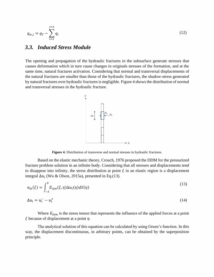
and transversal stresses in the hydraulic fracture.

Figure 4. Distribution of transverse and normal stresses in hydraulic fractures.

Based on the elastic mechanic theory, Crouch, 1976 proposed the DDM for the pressurized

fracture problem solution in an infinite body. Considering that all stresses and displacements tend

to disappear into infinity, the stress distribution at point 𝜉 in an elastic region is a displacement

integral ∆𝑢𝑖 (Wu & Olson, 2015a), presented in Eq.(13).

𝜎𝑙𝑘(𝜉) = ∫ 𝐸𝑙𝑗𝑚(𝜉, 𝜂)∆𝑢𝑙(𝜂)𝑑𝑆(𝜂)𝑆

−𝑆

(13)

∆𝑢𝑙 = 𝑢𝑙− − 𝑢𝑙

+

(14)

Where 𝐸𝑙𝑘𝑚 is the stress tensor that represents the influence of the applied forces at a point

𝜉 because of displacement at a point 𝜂.

The analytical solution of this equation can be calculated by using Green’s function. In this

way, the displacement discontinuous, in arbitrary points, can be obtained by the superposition

principle.

Because of the complexity of the analytical solution to Eq. (13), Crouch, 1976 developed

a numerical solution for this type of problem. The numerical solution of the DDM states that the

fracture must be replaced by N normal and transversal discontinuous displacements of unknown

magnitude. Thus, the total transversal and normal discontinuous displacement in the middle point

of the segment 𝑖𝑡ℎ is given by Eqs. (15)(16) (Crouch, 1976).

(𝜎𝑡)𝑙 = 𝑛𝑙𝑙𝑙 [(𝜎𝑥𝑥)𝑙 − (𝜎𝑦𝑦)𝑙] + (𝑛𝑙

2 − 𝑙𝑙2)(𝜎𝑥𝑦)

𝑙

(15)

(𝜎𝑛)𝑙 = 𝑙𝑙2(𝜎𝑥𝑥)𝑙 + 𝑛𝑙

2(𝜎𝑦𝑦)𝑙+ 2𝑛𝑙𝑙𝑙(𝜎𝑥𝑦)

𝑙

(16)

According to the DDM, the other elements influence over element 𝑖 can be written as linear

system of N equilibrium equations with N unknown parameters (�̂�𝑛, �̂�𝑡) system Eqs. (17)(18).

(𝜎𝑡)𝑙 = ∑ 𝐺𝑙𝑘(𝐴𝑡𝑡)𝑙𝑘(�̂�𝑡)𝑘 + ∑ 𝐺𝑙𝑘(𝐴𝑡𝑛)𝑙𝑘(�̂�𝑛)𝑘

𝑁

𝑘=1

𝑁

𝑘=1

(17)

(𝜎𝑛)𝑙 = ∑ 𝐺𝑙𝑘(𝐴𝑛𝑡)𝑙𝑘(�̂�𝑡)𝑘 + ∑ 𝐺𝑙𝑘(𝐴𝑛𝑛)𝑙𝑘(�̂�𝑛)𝑘

𝑁

𝑘=1

𝑁

𝑘=1

(18)

Where 𝐺𝑙𝑘 is the correction factor for 3D approximations derived by Olson (Olson, 2004)

and is presented in Eq.(19).

𝐺𝑙𝑘 = 1 −𝑑𝑙𝑘

𝛽

[𝑑𝑙𝑘2 + (ℎ 𝛼⁄ )

2

]

𝛽2⁄

(19)

With 𝛼 = 1 and 𝛽 = 2.3, which were empirically determined for a better adjustment of the

correction factor by Olson, 2004.

The boundary conditions (Eqs. (20)(21)) for stress or displacement are defined along the

fracture surface. These conditions involve the remote stress at the boundary, and the stress

generated for mechanic interaction with other nearby elements (Ren, Lin, & Zhao, 2018).

(𝜎𝑡)𝑙 = 0 (20)

(𝜎𝑛)𝑙 = −𝑃𝑛𝑒𝑡𝑎 (𝑖)

(21)

Combining the initial conditions and the stress equilibrium equations, the transversal and

normal stresses can be calculated, in each, fracture element in a simultaneous way. Where the

normal stress, �̂�𝑛, is equal to hydraulic fracture width 𝑤𝑓.

4. Numerical Solution

For the geometry calculation, a symmetric distribution is assumed. Due to this symmetry, only one

wing of the fracture is going to be calculated. To obtain the total dimensions of the fractures, the

length must be duplicated.

4.1. Fracture Propagation Module using FDM

The FDM is used to solve the mass balance equation Eq. (4), which is, a second-order partial

differential equation that describes the pressure drop along the hydraulic fracture, taking into

account the fracturing fluid movement into a porous medium.

Some assumptions are considered in order to simplify the FDM implementation. The

formation is assumed to be isotropic and homogeneous, implying a constant 𝜎ℎ in all the formation.

Considered the left side of the Eq. (4), presented in Eq. (22).

𝜋

64𝜇 𝜕

𝜕𝑦{ℎ𝑓(𝑦)𝑤𝑓(𝑦)

3 𝜕[𝑃𝑓(𝑦) − 𝜎ℎ]

𝜕𝑦}

(22)

The term ℎ𝑓(𝑦)𝑤𝑓(𝑦)3 introduce a non-linearity to the expression written in Eq. (22), this

non-linearity is presented since the two factors are a function of y. This imposes that the second

derivative approximation cannot be applied directly.

In order to solve this problem, the hydraulic fracture must be discretized in n finite space

elements to discretize the expression Eq. (22). Additionally, a substitution is introduced. Figure 5

shows the index, elements positions, and lengths used for the discretization.

Figure 5. Discretized fracture structure in n finite elements.

The substitution consists of the aggrupation of terms presented in Eq. (23). The derivative

of U with respect to y is evaluated in the middle of the ith element.

𝑈 = ℎ𝑓𝑤𝑓3𝜕[𝑃𝑓(𝑦) − 𝜎ℎ]

𝜕𝑦→

𝜋

64𝜇(𝜕𝑈

𝜕𝑦)𝑖

(23)

Using a forward approach of the FDM, the derivative of U is approximated by Eq. (24),

which states that the approximation is the difference between the U expression evaluated at the

point 𝑖 + 1/2 and the U expression evaluated at the point 𝑖 − 1/2 divided by the distance between

them, 𝛥𝑦.

𝜋

64𝜇(𝜕𝑈

𝜕𝑦)𝑖

=𝑈𝑖+1/2 − 𝑈𝑖−1/2

𝛥𝑦

(24)

Replacing 𝑈 expression substitution and as it can be noticed, the pressure drop derivative

is located at the point 𝑖 + 1/2 and 𝑖 − 1/2. Using again the forward approach for this pressure

drop derivative Eq. (25) is obtained.

𝜋

64𝜇(𝜕𝑈

𝜕𝑦)𝑖

=𝜋

64𝜇

[ (ℎ𝑓𝑤𝑓

3)𝑖+

12

(𝑃𝑓𝑖+1 − 𝑃𝑓𝑖

𝛥𝑦) − (ℎ𝑓𝑤𝑓

3)𝑖−

12

(𝑃𝑓𝑖 − 𝑃𝑓𝑖−1

𝛥𝑦)

𝛥𝑦

]

(25)

Assuming, q, a constant flow in the space element, can be utilized a transmissibility concept

(Mark W. McClure and Roland N. Horne, 2013). The fracture fluid transmissibility

𝑇𝑖+1/2, and 𝑇𝑖−1/2 in each cell edge are presented in Eq. (26) and Eq. (27).

𝑇𝑖+1/2 =𝜋

32𝜇𝛥𝑦 (

(ℎ𝑓𝑤𝑓3)

𝑖(ℎ𝑓𝑤𝑓

3)𝑖+1

(ℎ𝑓𝑤𝑓3)

𝑖+1+ (ℎ𝑓𝑤𝑓

3)𝑖

)

(26)

𝑇𝑖−1/2 =𝜋

32𝜇𝛥𝑦 (

(ℎ𝑓𝑤𝑓3)

𝑖−1(ℎ𝑓𝑤𝑓

3)𝑖

(ℎ𝑓𝑤𝑓3)

𝑖+ (ℎ𝑓𝑤𝑓

3)𝑖−1

)

(27)

Finally, Eq. (26) and Eq. (27) are replaced into Eq. (25), this obtaining Eq. (28). Appendix

A describes in detail the step-by-step solution for this part.

𝜋

64𝜇

𝜕

𝜕𝑦(ℎ𝑓𝑤𝑓

3𝜕[𝑃𝑓 − 𝜎ℎ]

𝜕𝑦)

𝑖

=

𝑇𝑖+

12(𝑃𝑓𝑖+1 − 𝑃𝑓𝑖) − 𝑇

𝑖−12(𝑃𝑓𝑖 − 𝑃𝑓𝑖−1)

𝛥𝑦

(28)

To apply the FDM to the right side of Eq. (4), which is a first-order partial derivate

equation, a forward approximate is implemented for the time derivative of the expression. The

result is written in Eq. (29).

2ℎ𝑓𝑖𝑛 𝐶𝐿

√𝑡 − 𝜏+

𝜋

4

2ℎ𝑓𝑛+1𝑤𝑓

𝑛+1 − ℎ𝑓𝑛+1𝑤𝑓

𝑛 − 𝑤𝑓𝑛+1ℎ𝑓

𝑛

𝑑𝑡

(29)

Since the time dependence is solved with an implicit form, the calculation of the fracturing

fluid pressure into a formation is done at the 𝑛 + 1 time step. To solve the implicit system, it is

required the pressure distribution, width, and height fracture at the 𝑛𝑡ℎ time step. The result is

written in Eq. (30).

𝑇𝑖+1/2𝑛+1(𝑃𝑓𝑖+1

𝑛+1 − 𝑃𝑓𝑖𝑛+1) − 𝑇𝑖−1/2

𝑛+1(𝑃𝑓𝑖𝑛+1 − 𝑃𝑓𝑖−1

𝑛+1)

𝛥𝑦

=2ℎ𝑓𝑖

𝑛 𝐶𝐿

√𝑡 − 𝜏+

𝜋

4 [

2ℎ𝑓𝑛+1𝑤𝑓

𝑛+1 − ℎ𝑓𝑛+1𝑤𝑓

𝑛 − 𝑤𝑓𝑛+1ℎ𝑓

𝑛

𝛥𝑡]

(30)

Finally, the solution of the implicit system, allows obtaining the fracture pressure changes

in space and time, incorporating the properties of the formation.

The positive transmissibility must be terminated with the limit as the net pressure tends to

zero since the positive transmissibility expression evaluated at this point is undetermined. The

resulting expression is written in Eq. (31) and is used as a fracture termination condition.

lim𝑃𝑛(𝑖+1)→0

𝑇𝑖+1/2 =𝐾𝐼𝐶

2𝑤𝑓𝑖3

16𝜇𝛥𝑦𝑃𝑛𝑒𝑡𝑎2

(31)

Boundary condition approximation

The boundary condition written in Eq. (5) is forward derivative approximated, obtaining eq. (32).

𝑃𝑓𝑖 = 𝑃𝑖𝑛𝑦 −64𝜇𝑄𝑖∆𝑦

𝜋ℎ𝑓(𝑖)𝑤𝑓(𝑖)3

(32)

4.2. Flow Rate Distribution Module solving a Non-linear Equation

System

Considering the friction of the fracturing fluid flow, the inlet flow rates are different for each

hydraulic fracture. Solving the square nonlinear system described by equations (9) and (12) these

flow rates are calculated (Rushing, 2006).

𝑞𝑇 − ∑𝑞𝑖

𝑗=1

𝑖=1

= 0

(33)

𝑃𝑓𝑖.𝑓 + ∆𝑃𝑝𝑓,𝑓 + ∑∆𝑃𝑤,𝑗 − 𝑃ℎ𝑒𝑒𝑙 = 0

𝑖

𝑗=1

(34)

The nonlinear system obtained is a 𝑁 + 1 square system, with the calculation of the

equation (34) for each hydraulic fracture (𝑁) and the equation (33) the square system is completed.

An interior point optimization solver is implemented in Python to solve this system.

4.3. Formation Stress Module using DDM

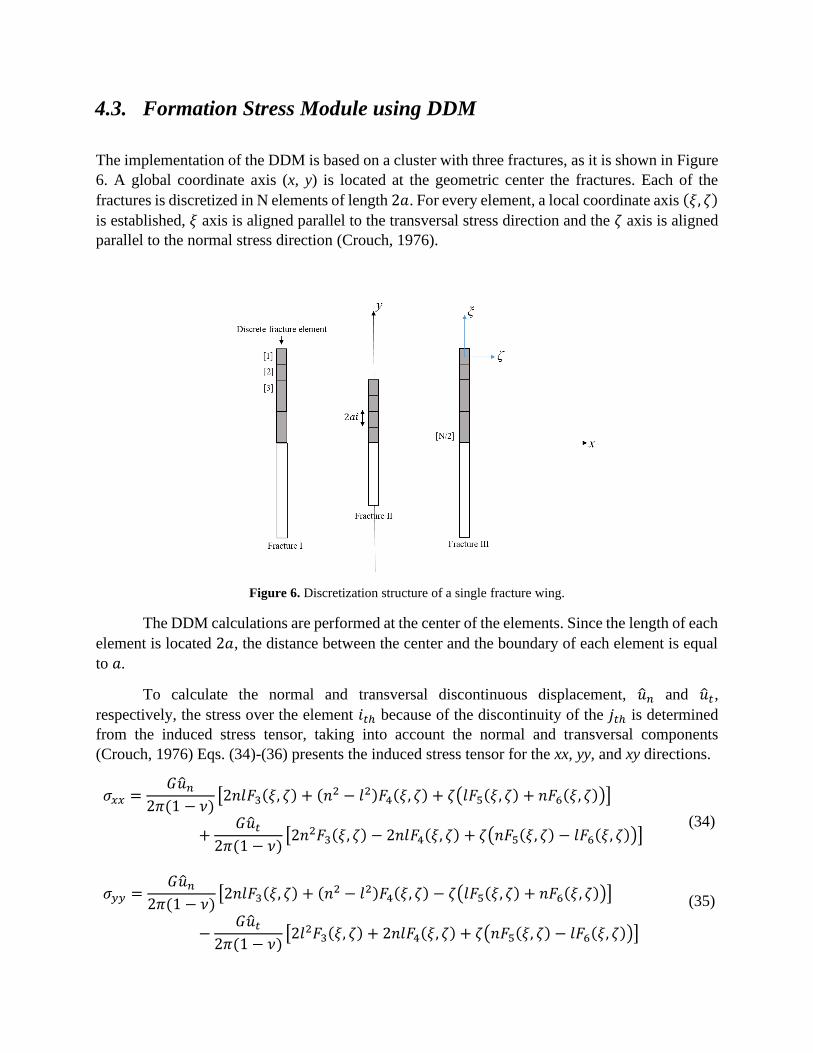
The implementation of the DDM is based on a cluster with three fractures, as it is shown in Figure

6. A global coordinate axis (x, y) is located at the geometric center the fractures. Each of the

fractures is discretized in N elements of length 2𝑎. For every element, a local coordinate axis (𝜉, 𝜁)

is established, 𝜉 axis is aligned parallel to the transversal stress direction and the 𝜁 axis is aligned

parallel to the normal stress direction (Crouch, 1976).

Figure 6. Discretization structure of a single fracture wing.

The DDM calculations are performed at the center of the elements. Since the length of each

element is located 2𝑎, the distance between the center and the boundary of each element is equal

to 𝑎.

To calculate the normal and transversal discontinuous displacement, �̂�𝑛 and �̂�𝑡,

respectively, the stress over the element 𝑖𝑡ℎ because of the discontinuity of the 𝑗𝑡ℎ is determined

from the induced stress tensor, taking into account the normal and transversal components

(Crouch, 1976) Eqs. (34)-(36) presents the induced stress tensor for the xx, yy, and xy directions.

𝜎𝑥𝑥 =𝐺�̂�𝑛

2𝜋(1 − 𝜈)[2𝑛𝑙𝐹3(𝜉, 𝜁) + (𝑛2 − 𝑙2)𝐹4(𝜉, 𝜁) + 𝜁(𝑙𝐹5(𝜉, 𝜁) + 𝑛𝐹6(𝜉, 𝜁))]

+𝐺�̂�𝑡

2𝜋(1 − 𝜈)[2𝑛2𝐹3(𝜉, 𝜁) − 2𝑛𝑙𝐹4(𝜉, 𝜁) + 𝜁(𝑛𝐹5(𝜉, 𝜁) − 𝑙𝐹6(𝜉, 𝜁))]

(34)

𝜎𝑦𝑦 =𝐺�̂�𝑛

2𝜋(1 − 𝜈)[2𝑛𝑙𝐹3(𝜉, 𝜁) + (𝑛2 − 𝑙2)𝐹4(𝜉, 𝜁) − 𝜁(𝑙𝐹5(𝜉, 𝜁) + 𝑛𝐹6(𝜉, 𝜁))]

−𝐺�̂�𝑡

2𝜋(1 − 𝜈)[2𝑙2𝐹3(𝜉, 𝜁) + 2𝑛𝑙𝐹4(𝜉, 𝜁) + 𝜁(𝑛𝐹5(𝜉, 𝜁) − 𝑙𝐹6(𝜉, 𝜁))]

(35)

𝜎𝑥𝑦 =𝐺�̂�𝑛

2𝜋(1 − 𝜈)𝜁(𝑙𝐹6(𝜉, 𝜁) − 𝑛𝐹5(𝜉, 𝜁))

+𝐺�̂�𝑡

2𝜋(1 − 𝜈)[𝐹4(𝜉, 𝜁) + 𝜁(𝑙𝐹5(𝜉, 𝜁) + 𝑛𝐹6(𝜉, 𝜁))]

(36)

Where 𝐺 is the shear modulus of material, and it can be calculated with Eq. (37) (J. Hu et

al., 2016)

𝐺 =𝐸

2(1 + 𝜈)

(37)

The 𝑙𝑙, and 𝑛𝑙 terms are the directions cosines of the normal vector to the fracture surface,

with respect with the global axis (𝑥, 𝑦). Figure 7 depicts the directions and the calculations for

these terms.

Figure 7. Defining the position, size, and orientation of discontinuous displacements.

The local coordinate system values (𝜉, 𝜁) are calculated with the direction cosines

and the global coordinates of the 𝑖𝑡ℎ element. This (𝜉, 𝜁) system is obtained by using Eqs.

(38) and (39).

𝜉𝑙 = 𝑛𝑘(𝑥𝑙 − 𝑥𝑘) − 𝑙𝑘(𝑦𝑙 − 𝑦𝑘) (38)

𝜁𝑙 = 𝑙𝑘(𝑥𝑙 − 𝑥𝑘) + 𝑛𝑘(𝑦𝑙 − 𝑦𝑘)

(39)

Finally, the 𝐹(𝜉, 𝜁) functions are calculated with the expressions derived by Crouch, 1976,

and are presented in appendix B.

With the total induced stresses calculations Eqs. (34)-(36), Eq. (15) and (16) can be

obtained for each 𝑖𝑡ℎ element. Then, these expressions are reorganized, gathering the terms that

multiplies the transversal displacements �̂�𝑡 and the normal displacements �̂�𝑛. After the terms

reorganization, (𝐴𝑡𝑡)𝑙𝑘, (𝐴𝑡𝑛)𝑙𝑘, (𝐴𝑛𝑡)𝑙𝑘, (𝐴𝑛𝑛)𝑙𝑘 values can be extracted. The calculation of these

values is presented in appendix C.

Finally, the equilibrium equations, Eqs. (17) and (18), are solved in order to obtain the

unknown parameters �̂�𝑛, �̂�𝑡. The linear system is established with the initial conditions described

by Eqs. (20) and (21). The �̂�𝑛 value corresponds to the fracture width, that can be replaced into

the FDM, in the mass balance equation discretization (Eq. (30)).

4.4. Coupling the models

The three modules flow charts are presented in Figure 8. for the flow rate distribution module, in

Figure 9. for the formation stress module, and in Figure 10. for the fracture propagation module.

The flow chart of the coupling of the three modules is presented in Figure 11.

Figure 8. Flow rate distribution module flow chart.

The flow rates at each hydraulic fracture are calculated by solving the non-linear equation

system presented in Eq. (33) and Eq. (34). To solve this non-linear equation system, the wellbore

parameters and the initialization parameters are required. The initialization variables are obtained

with the solution of the discretized boundary condition written in Eq. (32). Once the flow rates are

calculated, a criterion is evaluated. If one of the flow rates is negative, the initialization parameters

produce and infeasible solution scenario. This infeasibility is raised when a non-physical behavior

is described by the input parameters.

Figure 9. Formation stress module flow chart.

The Formation Stress Module requires the geological parameters. The number of fractures

and the discretization along them are required for the global coordinates (𝑥, 𝑦) calculation of the

discretization grid. With this information, the formation stress module calculates the coefficients

(𝐴𝑡𝑡)𝑙𝑘, (𝐴𝑡𝑛)𝑙𝑘, (𝐴𝑛𝑡)𝑙𝑘, (𝐴𝑛𝑛)𝑙𝑘 and the [𝐴𝑙,𝑘] matrix is obtained. Using this matrix, the fracture

width 𝑤𝑓 can be obtained by solving the linear system given by Eq. (40).

[[𝐴𝑡𝑡] [𝐴𝑡𝑛]

[𝐴𝑡𝑛] [𝐴𝑛𝑛]]−1

[0

[−𝑃𝑛]] = [[�̂�𝑡]

[𝑊𝑓]]

(40)

If the inverse matrix is singular, a correction on the input variables must be done in order

to obtain a feasible solution of the module.

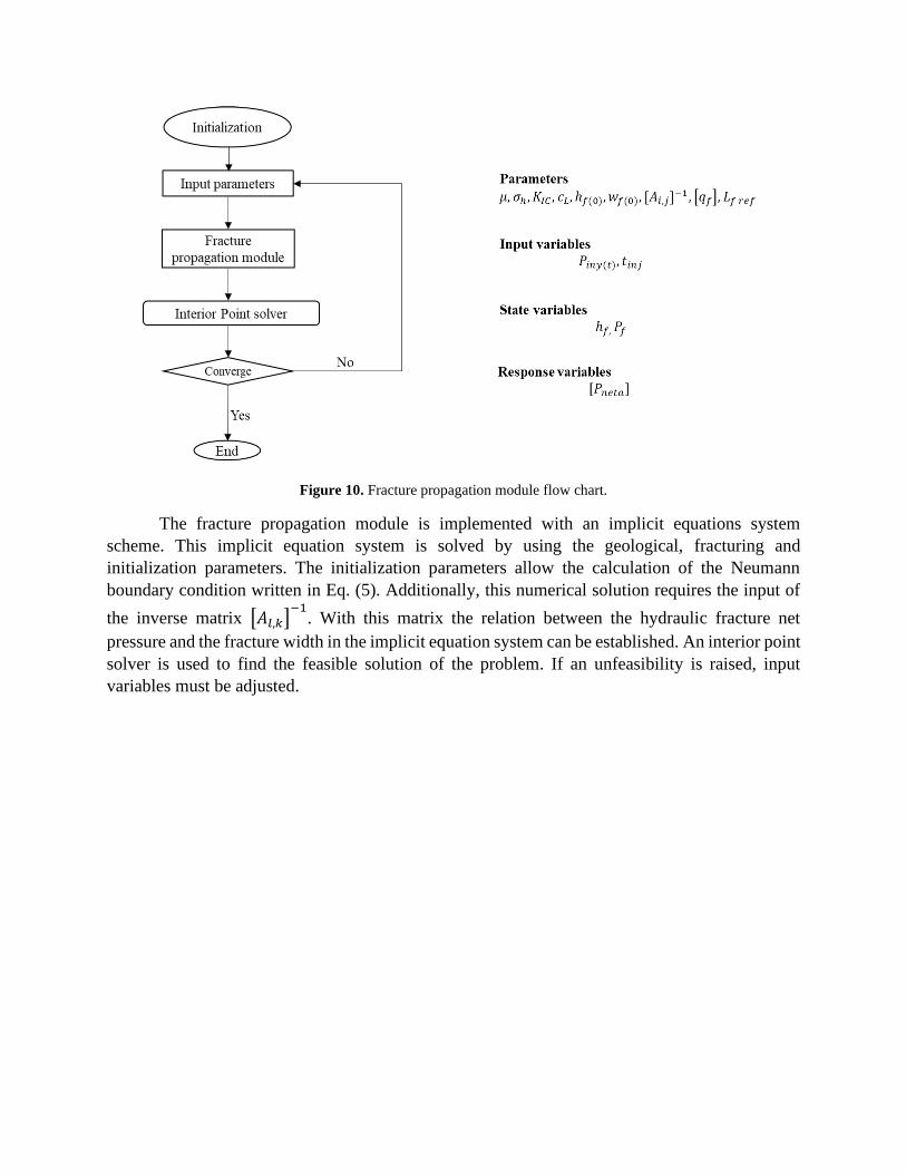
Figure 10. Fracture propagation module flow chart.

The fracture propagation module is implemented with an implicit equations system

scheme. This implicit equation system is solved by using the geological, fracturing and

initialization parameters. The initialization parameters allow the calculation of the Neumann

boundary condition written in Eq. (5). Additionally, this numerical solution requires the input of

the inverse matrix [𝐴𝑙,𝑘]−1

. With this matrix the relation between the hydraulic fracture net

pressure and the fracture width in the implicit equation system can be established. An interior point

solver is used to find the feasible solution of the problem. If an unfeasibility is raised, input

variables must be adjusted.

Figure 11. Models coupling diagram.

The three modules described above are coupled to obtain the hydraulic fracture geometry

for multiple fractures and multiple fracturing stages in a simultaneous scheme. The diagram

depicted in Figure 11 describes the interaction between the three numerical solutions and the input

parameters for the implemented numerical simulation.

To complete the first implicit equation system, the fracture propagation module must be

coupled with the flow rate distribution module to obtain the flow rates of each hydraulic fracture.

The initialization is the same for the flow rates module and the FDM since the inlet pressure of the

hydraulic fractures is required by the two modules. With a suitable initialization, the first implicit

equation system (FDM) can be solved, and the fracture length criterion can be evaluated.

Since the hydraulic fracture lengths are not modeled by analytical expressions, the model

cannot predict its behavior. A fracture length criterion is implemented with two implicit equation

systems. This criterion determines whether the fracture propagates according to the net pressure

along the fracture. In other words, the hydraulic fracture propagates while the net pressure on the

𝑖𝑡ℎ element of the fracture is greater than the maximum horizontal stress 𝜎𝐻 (Economides & Nolte,

2000). The initialization of the fracture length (𝐿𝑓 𝑟𝑒𝑓), provided to the first implicit equation

system, is a reference length that allows the fractures to propagate in an unconstrained way along

with the discretized domain.

With the solution of the first implicit equation system, the length of the hydraulic fractures

is obtained upon the criterion. With these values, the hydraulic fracture propagation, in the second

implicit equation system, is constrained to propagate until this point.

The geometry of the hydraulic fractures is obtained by solving the second implicit equation

system, using the inverse matrix [𝐴𝑙,𝑘]−1

, the flow rates of each hydraulic fracture, and the

hydraulic fracture lengths.

5. Case of study

The numerical solution described in section 4 is implemented on the Fuling shale gas field located

in the Sichuan Basin, southwest China and it is modeled by the parameters found in literature and

presented in Table 2.

5.1. Geological and Fracturing Parameters

Table 2 contains the geological properties of the Fuling shale gas field and the different operations

conditions for the hydraulic fracturing.

Table 2. Geological and fracturing parameters.

Parameters Value Unit Ref

Thickness 38 𝑚

Ren, Lin, & Zhao, 2018

Depth 2538–2576 𝑚

Initial reservoir pressure 38 𝑀𝑃𝑎

Young’s modulus 33 𝐺𝑃𝑎

Poisson’s ratio 0.21 --

Maximum horizontal stress 61.5 𝑀𝑃𝑎

Minimum horizontal stress 52.4 𝑀𝑃𝑎

Vertical stress 58.5 𝑀𝑃𝑎

Viscosity fluid fracturing 9 𝑚 ∙ 𝑃𝑎 ∙ 𝑠

Pump rate 13 m3

s⁄

Pump duration 123 𝑚𝑖𝑛

Cluster spacing 30 𝑚

Number of clusters 3 𝑁𝑢𝑚𝑏𝑒𝑟

Fracture toughness 2.5 𝑀𝑃𝑎 ∙ 𝑚0.5 Thiercelin et al., 1987

5.2. Wellbore Parameters

Table 3 show wellbore information used in the hydraulic fracturing in the field of study.

Table 3.Wellbore parameters.

Parameters Value Unit Ref

Perforation number 16 --

Ren, Lin, Zhao, et al., 2018

Perforation diameter 0.008 𝑚

Perforation flow coefficient 0.85 --

Wellbore diameter 0.1186 𝑚

Well segment length 30 𝑚

5.3. Single Hydraulic Fracture Solution

Two sets are declared for the solution of this problem, the first one is the set of elements related to

the space discretization of the hydraulic fracturing (𝐼 = {1, 2, 3…𝑁}). The second set is related to

the time discretization (𝑇 = {1, 2, 3…𝑇ℎ}). The structure of the fracture is discretized in space

from the 1 to the 𝑁 − 1 element, considering that the Nth element correspond to the boundary

condition.

For this study, a 𝑁 = 50 with a space discretization of ∆𝑦 = 4.32 𝑚 constitutes the

discretization of the fracture. Additionally, for the time discretization, the injection time interval

of 6660 𝑠𝑒𝑐𝑜𝑛𝑑𝑠 is divided in 20-time steps with ∆𝑡 = 333 𝑠. The total flow rate 𝑞𝑡 for this

fracture is 2.172 𝑚3

𝑠⁄ (Ren, Lin, Zhao, et al., 2018).

The results from the models coupling for a single hydraulic fracture is shown in the Figure

12, which describes the net pressure behavior, the fracture width and the fracture half-length at the

ultimate time step.

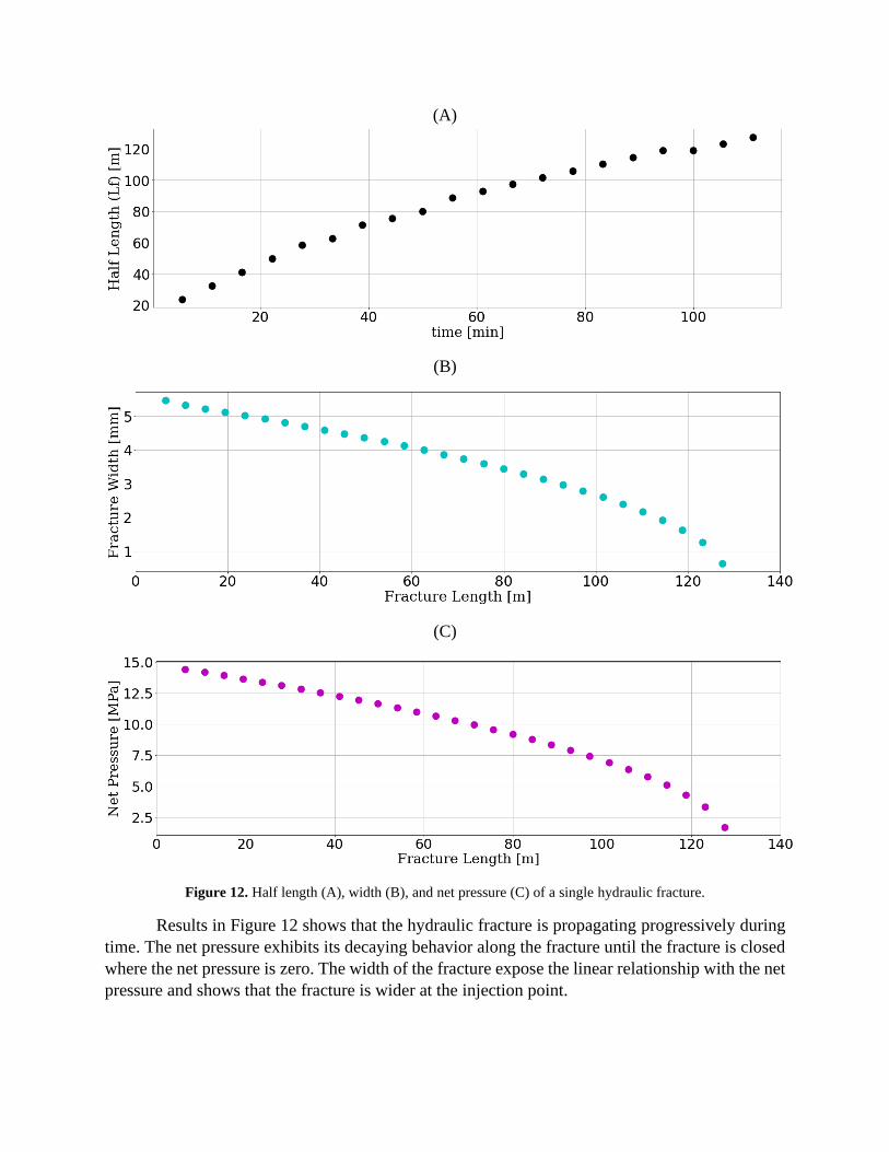
(A)

(B)

(C)

Figure 12. Half length (A), width (B), and net pressure (C) of a single hydraulic fracture.

Results in Figure 12 shows that the hydraulic fracture is propagating progressively during

time. The net pressure exhibits its decaying behavior along the fracture until the fracture is closed

where the net pressure is zero. The width of the fracture expose the linear relationship with the net

pressure and shows that the fracture is wider at the injection point.

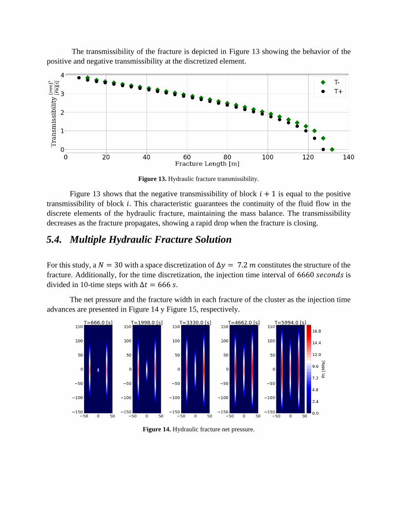
The transmissibility of the fracture is depicted in Figure 13 showing the behavior of the

positive and negative transmissibility at the discretized element.

Figure 13. Hydraulic fracture transmissibility.

Figure 13 shows that the negative transmissibility of block 𝑖 + 1 is equal to the positive

transmissibility of block 𝑖. This characteristic guarantees the continuity of the fluid flow in the

discrete elements of the hydraulic fracture, maintaining the mass balance. The transmissibility

decreases as the fracture propagates, showing a rapid drop when the fracture is closing.

5.4. Multiple Hydraulic Fracture Solution

For this study, a 𝑁 = 30 with a space discretization of ∆𝑦 = 7.2 𝑚 constitutes the structure of the

fracture. Additionally, for the time discretization, the injection time interval of 6660 𝑠𝑒𝑐𝑜𝑛𝑑𝑠 is

divided in 10-time steps with ∆𝑡 = 666 𝑠.

The net pressure and the fracture width in each fracture of the cluster as the injection time

advances are presented in Figure 14 y Figure 15, respectively.

Figure 14. Hydraulic fracture net pressure.

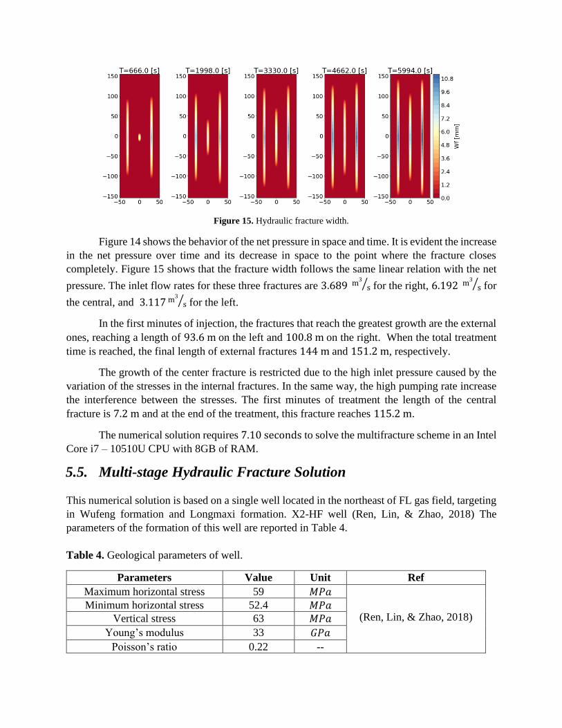
Figure 15. Hydraulic fracture width.

Figure 14 shows the behavior of the net pressure in space and time. It is evident the increase

in the net pressure over time and its decrease in space to the point where the fracture closes

completely. Figure 15 shows that the fracture width follows the same linear relation with the net

pressure. The inlet flow rates for these three fractures are 3.689 m3

s⁄ for the right, 6.192 m3

s⁄ for

the central, and 3.117 m3

s⁄ for the left.

In the first minutes of injection, the fractures that reach the greatest growth are the external

ones, reaching a length of 93.6 m on the left and 100.8 m on the right. When the total treatment

time is reached, the final length of external fractures 144 m and 151.2 m, respectively.

The growth of the center fracture is restricted due to the high inlet pressure caused by the

variation of the stresses in the internal fractures. In the same way, the high pumping rate increase

the interference between the stresses. The first minutes of treatment the length of the central

fracture is 7.2 m and at the end of the treatment, this fracture reaches 115.2 m.

The numerical solution requires 7.10 seconds to solve the multifracture scheme in an Intel

Core i7 – 10510U CPU with 8GB of RAM.

5.5. Multi-stage Hydraulic Fracture Solution

This numerical solution is based on a single well located in the northeast of FL gas field, targeting

in Wufeng formation and Longmaxi formation. X2-HF well (Ren, Lin, & Zhao, 2018) The

parameters of the formation of this well are reported in Table 4.

Table 4. Geological parameters of well.

Parameters Value Unit Ref

Maximum horizontal stress 59 𝑀𝑃𝑎

(Ren, Lin, & Zhao, 2018) Minimum horizontal stress 52.4 𝑀𝑃𝑎

Vertical stress 63 𝑀𝑃𝑎

Young’s modulus 33 𝐺𝑃𝑎

Poisson’s ratio 0.22 --

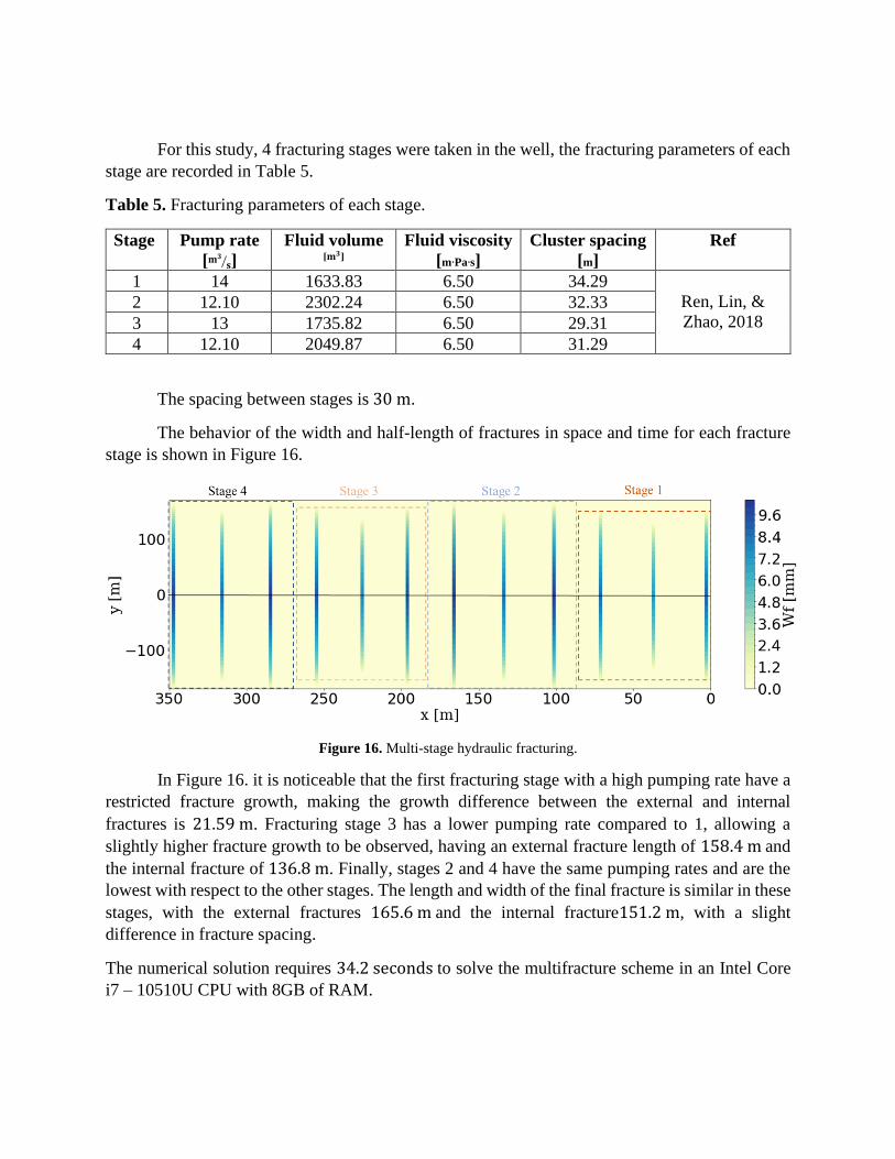
For this study, 4 fracturing stages were taken in the well, the fracturing parameters of each

stage are recorded in Table 5.

Table 5. Fracturing parameters of each stage.

Stage Pump rate

[𝐦𝟑

𝐬⁄ ]

Fluid volume [𝐦𝟑]

Fluid viscosity

[m∙Pa∙s]

Cluster spacing

[m]

Ref

1 14 1633.83 6.50 34.29

Ren, Lin, &

Zhao, 2018 2 12.10 2302.24 6.50 32.33

3 13 1735.82 6.50 29.31

4 12.10 2049.87 6.50 31.29

The spacing between stages is 30 m.

The behavior of the width and half-length of fractures in space and time for each fracture

stage is shown in Figure 16.

Figure 16. Multi-stage hydraulic fracturing.

In Figure 16. it is noticeable that the first fracturing stage with a high pumping rate have a

restricted fracture growth, making the growth difference between the external and internal

fractures is 21.59 m. Fracturing stage 3 has a lower pumping rate compared to 1, allowing a

slightly higher fracture growth to be observed, having an external fracture length of 158.4 m and

the internal fracture of 136.8 m. Finally, stages 2 and 4 have the same pumping rates and are the

lowest with respect to the other stages. The length and width of the final fracture is similar in these

stages, with the external fractures 165.6 m and the internal fracture151.2 m, with a slight

difference in fracture spacing.

The numerical solution requires 34.2 seconds to solve the multifracture scheme in an Intel Core

i7 – 10510U CPU with 8GB of RAM.

6. Discussion

The proposed simultaneous numerical solution well approximates the physical phenomenon of the

unconventional hydraulic fracturing process. Furthermore, the fracture propagation module

exhibits a progressive growth of hydraulic fractures during the injection time. Additionally, the

transmissibility behavior shows a continuous fluid flow along the hydraulic fracture, validating the

implementation of the pressure drop equation. In the same way, the net pressure behavior in space

and time is an accurate model of the real behavior of this variable.

The calculated fracture widths for the study case show a linear relation with the hydraulic

fracture net pressure. This behavior is sustained on the fact that the formation stress model is a

linear equation system, making the hydraulic fracture behave as the presented geometry in section

2, a long and narrow hydraulic fracture. The obtained results show that the fracture width is

independent of the fracture length.

According to the flow rate distribution model, three fractures are propagated

simultaneously with different flow rates during multiple hydraulic fracturing. This model implies

that the central hydraulic fracture flow rate is higher than the flow rates of the external hydraulic

fractures. With higher inlet flow rates, the net pressure increases, increasing the stress interference.

In a high-stress interference scenario, the growth of the central hydraulic fracture is limited. This

showed that the pumping rate of each hydraulic fracture is an important variable that determines

the fracture length.

The multistage hydraulic fracturing solution shows that, with homogeneous and isotropic

geological conditions, the stress interference is more evident. Generating higher net pressures in

the hydraulic fractures of the process, and therefore the propagation of the fractures is restricted

during the development of the multiple stages. In the same way, the pumped flow rates show that

its variations are decisive to the hydraulic fracture growth.

The importance of the flow rate distribution initialization is due to the dependence of the

inlet flow rates of the hydraulic fractures and their growth. The initialization of the model allows

obtaining a feasible problem that complies with the physical behaviors of unconventional

hydraulic fracturing. With the adjustment of the injected pressure parameter, accurate flow rates

can be obtained according to the limitations of the process. In the same way, an initialization

criterion can be established for the adequate input of the initialization parameters.

The simultaneous numerical solution implemented in this work allows the selection of the

appropriate fracturing pressure (injected pressure) during the design of the hydraulic fracturing

process. With these fracturing pressure curves, the geometries of hydraulic fractures, the fracture

propagation. and its distribution within the formation can be obtained. The numerical solution also

allows the evaluation of multiple hydraulic fracture distributions with different orientations to

calculate their effects on the formation stress interference.

As future work, the Stimulated Reservoir Volume (SRV) can be obtained from the

simultaneous numerical simulation implemented. The calculation of SRV requires the

implementation of the pressure distribution model and the natural fracture failure criterion. The

pressure distribution model is calculated from the reservoir pressure changes due to the modelled

leak-off in the fracture propagation model. The natural fracture failure criterion is based on the

changes in the formation stresses, calculated with the formation stress model. This implementation

should take advantage of the reduced simulation times achieved in this study.

The simultaneous numerical simulation strategy reduces simulation times drastically for

the fracture geometry and distribution calculation. For example, a multiple fracture (3 fractures)

scenario requires 9.55 seconds to obtain the multiple hydraulic fracture geometry such the one

presented in Figure 17. A multistage (15 stages) scenario requires 156.70 seconds. As a reference

for the simulation time, the work of Ren, Lin, & Zhao, 2018 takes 587 seconds to calculate the

SRV for a single stage with 3 fractures. Considering that this work does not calculate the SRV, the

times cannot be compared directly. However, it is a promising result since the pressure distribution

model and the natural fracture failure criterion are low-computational cost models (Ren, Lin, &

Zhao, 2018).

Figure 17. Fracture width at the ultimate time step.

Finally, with a time-reduced simulation scheme such as the one presented in this work; an

optimization problem can be solved in an agile way. Multiple works in literature that maximize

the fracture length and the number of fracturing stages to obtain the maximum SRV (Lin, Ren,

Zhao, Wu, et al., 2017). Some others maximize the net present value (NPV) obtained from the

formation treatment (Zhang & Sheng, 2020), (W. Yu et al., 2015), and (Zhang & Sheng, 2020). In

Table 6, the formulation of an optimization problem is presented, aiming to maximize the NPV of

the hydraulic fracturing process, with the optimal set of manipulable variables constrained by their

feasible variation ranges.

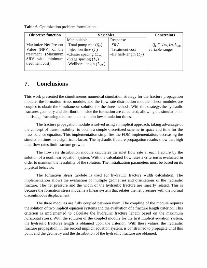
Table 6. Optimization problem formulation.

Objective function Variables Constraints

Manipulable Response

Maximize Net Present

Value (NPV) of the

treatment (Maximum

SRV with minimum

treatment cost)

-Total pump rate (𝑄𝑡)

-Injection time (𝑇)

-Cluster spacing (𝐿𝑤)

-Stage spacing (𝐿𝑠)

-Wellbore length (𝐿𝑤𝑏)

-𝑆𝑅𝑉

-Treatment cost

-HF half-length (𝐿𝑓)

- 𝑄𝑡, 𝑇, 𝐿𝑤, 𝐿𝑠, 𝐿𝑤𝑏

variable ranges

7. Conclusions

This work presented the simultaneous numerical simulation strategy for the fracture propagation

module, the formation stress module, and the flow rate distribution module. These modules are

coupled to obtain the simultaneous solution for the three methods. With this strategy, the hydraulic

fractures geometry and distribution inside the formation are calculated, allowing the simulation of

multistage fracturing treatments to maintain low simulation times.

The fracture propagation module is solved using an implicit approach, taking advantage of

the concept of transmissibility, to obtain a simple discretized scheme in space and time for the

mass balance equation. This implementation simplifies the FDM implementation, decreasing the

simulation times in a significant factor. The hydraulic fracture propagation results show that high

inlet flow rates limit fracture growth.

The flow rate distribution module calculates the inlet flow rate at each fracture by the

solution of a nonlinear equation system. With the calculated flow rates a criterion is evaluated in

order to maintain the feasibility of the solution. The initialization parameters must be based on its

physical behavior.

The formation stress module is used for hydraulic fracture width calculation. The

implementation allows the evaluation of multiple geometries and orientations of the hydraulic

fracture. The net pressure and the width of the hydraulic fracture are linearly related. This is

because the formation stress model is a linear system that relates the net pressure with the normal

discontinuous displacement.

The three modules are fully coupled between them. The coupling of the module requires

the solution of two implicit equation systems and the evaluation of a fracture length criterion. This

criterion is implemented to calculate the hydraulic fracture length based on the maximum

horizontal stress. With the solution of the coupled module for the first implicit equation system,

the hydraulic fractures length is obtained upon the criterion. With these values, the hydraulic

fracture propagation, in the second implicit equation system, is constrained to propagate until this

point and the geometry and the distribution of the hydraulic fracture are obtained.

The code implementation of this study is written in python as an open software that allows

the use of the simulator to carry out various technical and financial analyzes. With this software

an optimal design and development of the hydraulic fracturing treatment can be performed.

Nomenclature

Latin symbols: real terms

(𝐴𝑡𝑡)𝑙𝑘,(𝐴𝑡𝑛)𝑙𝑘, (𝐴𝑛𝑡)𝑙𝑘,(𝐴𝑛𝑛)𝑙𝑘 Elastic-influence coefficient matrix representing the

transversal/normal stress at element l induced by normal-displacement/transversal-displacement

at element k, respectively

𝑐𝐿 Filtration coefficient [m/s0.5]

𝑑 Wellbore diameter [m]

𝑑𝑙𝑘 Distance between fracture element l and fracture element k [m]

𝑑𝑝𝑓,𝑓 Perforation diameter [m]

𝐹3, 𝐹4, 𝐹5, 𝐹6 Derivatives functions

𝐺 Shear modulus [Pa]

𝐺𝑙𝑘 Correction factor of DDM

ℎ𝑓(𝑖) Fracture heigh [m]

𝐾𝐼𝐶 Fracture toughness [Pa ∙ m0.5]

𝐿𝑓 Fracture length [m]

𝑙𝑙 Cosines direction about the x-axis

𝐿𝑤,𝑗 Length of wellbore segment j [m]

𝑛′ Power-law index

𝑛𝑙 Cosines direction about the y-axis

𝑛𝑝𝑓,𝑓 Perforation number

𝑃𝑓(𝑖) Fluid pressure in fracture [m]

𝑃𝑓𝑖.𝑓 Inlet flow rate of hydraulic fracture i [m3/s]

𝑃ℎ𝑒𝑒𝑙 Pressure at horizontal wellbore heel [Pa]

𝑃𝑛𝑒𝑡𝑎 (𝑖) Net pressure in fracture [Pa]

𝑃0 Injection pressure [Pa]

𝑞𝑓 Flow rate at perforation [m3/s]

𝑞(𝑖) Flow rate in fracture [m3/s]

𝑞𝑤,𝑗 Flow rate of wellbore segment j [m3/s]

𝑞𝑇 Total flow rate [m3/s]

𝑄𝑓 Inflow rate in each fracture [m3/s]

𝑡 Time [s]

𝑇 Transmissibility [m3/Pa∙s]

𝑇ℎ Time horizon [min]

(�̂�𝑡)𝑘 Transversal stress at element k [m]

(�̂�𝑛)𝑘 Normal stress at element k [m]

𝑤𝑓(𝑖) Fracture width [m]

∆𝑃𝑝𝑓,𝑓 Perforation friction pressure drop of fracture f [Pa]

∆𝑃𝑤,𝑗 Wellbore friction pressure drop of segment j [Pa]

∆𝑡 Length of infinitesimal time element [s]

∆𝑢𝑙 Displacement integral [m]

∆𝑦 Length of infinitesimal fracture element [m]

Greek symbols

𝜇 Viscosity fracturing fluid [Pa∙s]

𝜎ℎ Minimum horizontal stress [Pa]

(𝜎𝑛)𝑙 Normal stress on element i in local coordinate [Pa]

𝜎𝑙𝑘 Stress distribution [Pa]

(𝜎𝑡)𝑙 Transversal stress on element i in local coordinate [Pa]

𝜎𝑥𝑥, 𝜎𝑦𝑦, 𝜎𝑥𝑦 Components of induced stress tensor [Pa]

𝜏(𝑖) Start time of leak-off in fracture [s]

𝜈 Poisson ratio

𝛼, 𝛽 Empirical constants

𝛼𝑝𝑓,𝑓 Flow coefficient of perforation, commonly ranged from 0.8 to 0.85 [dimensionless]

𝜌 Fracturing fluid density [Kg/m3]

Subscripts

𝑓 Index of fractures set

𝑖 Index of space discretization blocks set

𝑗 Index of wellbore segments set

𝑘 Index of discretization element in formation stress model

𝑙 Index of discretization interaction element in formation stress model

Superscripts

𝑛 Index of time discretization slots set

References

Crouch, S. L. (1976). Solution of plane elasticity problems by the displacement discontinuity

method. I. Infinite body solution. International Journal for Numerical Methods in

Engineering, 10(2), 301–343. https://doi.org/10.1002/nme.1620100206

Economides, M., & Nolte, Kenneth. (2000). Reservoir Stimulation. In Wiley New York.

Hu, J., Yang, S., Fu, D., Rui, R., Yu, Y., & Chen, Z. (2016). Rock mechanics of shear rupture in

shale gas reservoirs. Journal of Natural Gas Science and Engineering, 36, 943–949.

https://doi.org/10.1016/j.jngse.2016.11.033

Hu, Y., Li, Z., Zhao, J., Tao, Z., & Gao, P. (2017). Prediction and analysis of the stimulated

reservoir volume for shale gas reservoirs based on rock failure mechanism. Environmental

Earth Sciences, 76(15), 1–13. https://doi.org/10.1007/s12665-017-6830-3

Huang, J., Safari, R., Lakshminarayanan, S., Mutlu, U., & McClure, M. (2014). Impact of discrete

fracture network (DFN) reactivation on productive stimulated rock volume: Microseismic,

geomechanics and reservoir coupling. 48th US Rock Mechanics / Geomechanics Symposium

2014, 1, 594–610.

Li, X. G., Yi, L. P., & Yang, Z. Z. (2017a). Numerical model and investigation of simultaneous

multiple-fracture propagation within a stage in horizontal well. Environmental Earth

Sciences, 76(7). https://doi.org/10.1007/s12665-017-6579-8

Li, Z., Qi, Z., Yan, W., Xiao, Q., Xiang, Z., & Tao, Z. (2019). An equivalent mathematical model

for 2D stimulated reservoir volume simulation of hydraulic fracturing in unconventional

reservoirs. Energy Sources, Part A: Recovery, Utilization and Environmental Effects, 7036.

https://doi.org/10.1080/15567036.2019.1679286

Lin, R., Ren, L., Zhao, J., & Huang, J. (2017). Stimulated reservoir volume of multi-stage

fracturing in horizontal shale gas well: Modeling and application. Society of Petroleum

Engineers - SPE/IATMI Asia Pacific Oil and Gas Conference and Exhibition 2017, 2017-

Janua. https://doi.org/10.2118/186294-ms

Lin, R., Ren, L., Zhao, J., Wu, L., & Li, Y. (2017). Cluster spacing optimization of multi-stage

fracturing in horizontal shale gas wells based on stimulated reservoir volume evaluation.

Arabian Journal of Geosciences, 10(2). https://doi.org/10.1007/s12517-016-2823-x

Liu, J., Wang, J., Leung, C., & Gao, F. (2018). A multi-parameter optimization model for the

evaluation of shale gas recovery enhancement. Energies, 11(3).

https://doi.org/10.3390/en11030654

Mark W. McClure and Roland N. Horne. (2013). Discrete Fracture Network Modeling of

Hydraulic Stimulation Coupling Flow and Geomechanics.

Meyer, B. R., & Bazan, L. W. (2011). A discrete fracture network model for hydraulically induced

fractures: Theory, parametric and case studies. Society of Petroleum Engineers - SPE

Hydraulic Fracturing Technology Conference 2011, 1993, 571–606.

Olson, J. E. (2004). Predicting fracture swarms - The influence of subcritical crack growth and the

crack-tip process on joint spacing in rock. Geological Society Special Publication, 231, 73–

87. https://doi.org/10.1144/GSL.SP.2004.231.01.05

Olson, J. E., & Wu, K. (2012a). Sequential versus simultaneous multi-zone fracturing in horizontal

wells: Insights from a non-planar, multi-frac numerical model. Society of Petroleum

Engineers - SPE Hydraulic Fracturing Technology Conference 2012, 2011, 737–751.

Ren, L., Lin, R., & Zhao, J. (2018). Stimulated Reservoir Volume Estimation and Analysis of

Hydraulic Fracturing in Shale Gas Reservoir. Arabian Journal for Science and Engineering,

43(11), 6429–6444. https://doi.org/10.1007/s13369-018-3208-0

Ren, L., Lin, R., Zhao, J., Rasouli, V., Zhao, J., & Yang, H. (2018). Stimulated reservoir volume

estimation for shale gas fracturing: Mechanism and modeling approach. Journal of Petroleum

Science and Engineering, 166(January), 290–304.

https://doi.org/10.1016/j.petrol.2018.03.041

Rogers, S., Elmo, D., Dunphy, R., & Bearinger, D. (2010). Understanding hydraulic fracture

geometry and interactions in the Horn River Basin through DFN and numerical modeling.

Society of Petroleum Engineers - Canadian Unconventional Resources and International

Petroleum Conference 2010, 2, 1426–1437. https://doi.org/10.2118/137488-ms

Rushing, J. (2006). Numerical Model of Multilayer Fracture Treatments. SPE Reprint Series, 59.

Thiercelin, M., Jeffrey, R. G., & Naceur, K. ben. (1987). Influence of Fracture Toughness on the

Geometry of Hydraulic Fractures. Society of Petroleum Engineers of AIME, (Paper) SPE,

November, 441–452.

Weng, X., Kresse, O., Cohen, C., Wu, R., & Gu, H. (2011). Modeling of hydraulic-fracture-

network propagation in a naturally fractured formation. SPE Production and Operations,

26(4), 368–380. https://doi.org/10.2118/140253-PA

Wu, K., & Olson, J. E. (2015a). Simultaneous multifracture treatments: Fully coupled fluid flow

and fracture mechanics for horizontal wells. SPE Journal, 20(2), 337–346.

https://doi.org/10.2118/167626-PA

Yu, G., & Aguilera, R. (2012). 3D analytical modeling of hydraulic fracturing stimulated reservoir

volume. SPE Latin American and Caribbean Petroleum Engineering Conference

Proceedings, 2, 1332–1348. https://doi.org/10.2118/153486-ms

Yu, W., Varavei, A., & Sepehrnoori, K. (2015). Optimization of Shale Gas Production Using

Design of Experiment and Response Surface Methodology. Energy Sources, Part A:

Recovery, Utilization and Environmental Effects, 37(8), 906–918.

https://doi.org/10.1080/15567036.2013.812698

Zhang, H., & Sheng, J. (2020). Optimization of horizontal well fracturing in shale gas reservoir

based on stimulated reservoir volume. Journal of Petroleum Science and Engineering,

190(October 2019), 107059. https://doi.org/10.1016/j.petrol.2020.107059

ZHAO, J., CHEN, X., LI, Y., FU, B., & XU, W. (2017). Numerical simulation of multi-stage

fracturing and optimization of perforation in a horizontal well. Petroleum Exploration and

Development, 44(1), 119–126. https://doi.org/10.1016/S1876-3804(17)30015-0

Appendix A - Numerical Solution of Fracture Propagation

Model using Finite Difference Method

Considered the left side of the Eq. (4), presented in Eq. (A1).

𝜋

64𝜇 𝜕

𝜕𝑦{ℎ𝑓(𝑦)𝑤𝑓(𝑦)

3 𝜕[𝑃𝑓(𝑦) − 𝜎ℎ]

𝜕𝑦}

(A1)

First, a substitution is performed, as shown in Eq. (A2).

𝑈 = ℎ𝑓𝑤𝑓3𝜕[𝑃𝑓(𝑦) − 𝜎ℎ]

𝜕𝑦→

𝜋

64𝜇(𝜕𝑈

𝜕𝑦)𝑖

(A2)

Using a forward approach of the FDM, the derivative of U is approximated by Eq. (A3),

𝜋

64𝜇(𝜕𝑈

𝜕𝑦)𝑖

=𝑈𝑖+1/2 − 𝑈𝑖−1/2

𝛥𝑦

(A3)

Replacing 𝑈 expression, Eq. (A4) is obtained.

𝜋

64𝜇(𝜕𝑈

𝜕𝑦)𝑖

=𝜋

64𝜇

(ℎ𝑓(𝑦)𝑤𝑓(𝑦)3 )

𝑖+1/2(𝜕[𝑃𝑓(𝑦) − 𝜎ℎ]

𝜕𝑦)

𝑖+1/2

− (ℎ𝑓(𝑦)𝑤𝑓(𝑦)3 )

𝑖−1/2(𝜕[𝑃𝑓(𝑦) − 𝜎ℎ]

𝜕𝑦)𝑖−1/2

𝛥𝑦

(A4)

The pressure drop derivative is located at the point 𝑖 + 1/2 and 𝑖 − 1/2. Using again the forward

approach for this pressure drop derivative Eqs. (A5) (A6) are obtained.

(𝜕[𝑃𝑓(𝑦) − 𝜎ℎ]

𝜕𝑦)

𝑖+1/2

= 𝑃𝑓𝑖+1 − 𝑃𝑓𝑖

𝛥𝑦

(A5)

(𝜕[𝑃𝑓(𝑦) − 𝜎ℎ]

𝜕𝑦)

𝑖−1/2

= 𝑃𝑓𝑖 − 𝑃𝑓𝑖−1

𝛥𝑦

(A6)

Replacing the Eqs. (A5) (A6) into a Eq. (A4), Eq. (A7) is obtained.

𝜋

64𝜇(𝜕𝑈

𝜕𝑦)𝑖

=𝜋

64𝜇

[ (ℎ𝑓(𝑦)𝑤𝑓(𝑦)

3 )𝑖+

12

(𝑃𝑓𝑖+1 − 𝑃𝑓𝑖

𝛥𝑦) − (ℎ𝑓(𝑦)𝑤𝑓(𝑦)

3 )𝑖−

12

(𝑃𝑓𝑖 − 𝑃𝑓𝑖−1

𝛥𝑦)

𝛥𝑦

]

(A7)

To obtain the transmissibility (𝑇𝑖+1/2, and 𝑇𝑖−1/2) terms, the flow in a porous medium is calculated

from Darcy’s law. Assuming, q, a constant flow in the space element, the flow that goes from the

points 𝑖 to 𝑖 + 1/2, and from 𝑖 + 1/2 to 𝑖 + 1, are given by Eqs. (A8) (A9).

𝑞𝑖, 𝑖+1/2 = −𝜋(ℎ𝑓(𝑦)𝑤𝑓(𝑦)

3 )𝑖

64𝜇(

𝑃𝑓𝑖+

12− 𝑃𝑓𝑖

𝛥𝑦2

)

(A8)

𝑞𝑖+1/2, 𝑖+1 = −𝜋(ℎ𝑓(𝑦)𝑤𝑓(𝑦)

3 )𝑖+1

64𝜇(

𝑃𝑓𝑖+1 − 𝑃𝑓𝑖+

12

𝛥𝑦2

)

(A9)

Solving for the drop pressure between the point 𝑖 and 𝑖 + 1 and adding the Eqs. (A8) (A9), Eq.

(A10) is obtained.

𝑃𝑓𝑖 − 𝑃𝑓𝑖+1 =32𝜇𝑞𝛥𝑦

𝜋(

(ℎ𝑓(𝑦)𝑤𝑓(𝑦)3 )

𝑖+1+ (ℎ𝑓(𝑦)𝑤𝑓(𝑦)

3 )𝑖

(ℎ𝑓(𝑦)𝑤𝑓(𝑦93 )

𝑖(ℎ𝑓(𝑦)𝑤𝑓(𝑦)

3 )𝑖+1

)

(A10)

Then, the flow equation is given by Eq. (11).

𝑞 =𝜋

32𝜇𝛥𝑦 (

(ℎ𝑓(𝑦)𝑤𝑓(𝑦)3 )

𝑖(ℎ𝑓(𝑦)𝑤𝑓(𝑦)

3 )𝑖+1

(ℎ𝑓(𝑦)𝑤𝑓(𝑦)3 )

𝑖+1+ (ℎ𝑓(𝑦)𝑤𝑓(𝑦)

3 )𝑖

) (𝑃𝑓𝑖 − 𝑃𝑓𝑖+1)

(A11)

Finally, the transmissibility at the points 𝑖 + 1/2 and 𝑖 − 1/2 are presented in Eq. (A12) and

(A13).

𝑇𝑖+1/2 =𝜋

32𝜇𝛥𝑦 (

(ℎ𝑓(𝑦)𝑤𝑓(𝑦)3 )

𝑖(ℎ𝑓(𝑦)𝑤𝑓(𝑦)

3 )𝑖+1

(ℎ𝑓(𝑦)𝑤𝑓(𝑦)3 )

𝑖+1+ (ℎ𝑓(𝑦)𝑤𝑓(𝑦)

3 )𝑖

)

(A12)

𝑇𝑖−1/2 =𝜋

32𝜇𝛥𝑦 (

(ℎ𝑓(𝑦)𝑤𝑓(𝑦)3 )

𝑖−1(ℎ𝑓(𝑦)𝑤𝑓(𝑦)

3 )𝑖

(ℎ𝑓(𝑦)𝑤𝑓(𝑦)3 )

𝑖+ (ℎ𝑓(𝑦)𝑤𝑓(𝑦)

3 )𝑖−1

)

(A13)

Replacing the Eq. (12), and (13) into a Eq. (7), Eq. (14) is obtained.

𝜋

64𝜇

𝜕

𝜕𝑦(ℎ𝑓(𝑦)𝑤𝑓(𝑦)

3𝜕[𝑃𝑓(𝑦) − 𝜎ℎ]

𝜕𝑦)

𝑖

=

𝑇𝑖+

12(𝑃𝑓𝑖+1 − 𝑃𝑓𝑖) − 𝑇

𝑖−12(𝑃𝑓𝑖 − 𝑃𝑓𝑖−1)

𝛥𝑦

(A14)

The transmissibility presents an indirect dependence with the time due to the fracture height, ℎ𝑓(𝑦),

and fracture width, 𝑤𝑓(𝑦). When time dependence is included in the transmissibility equation, Eqs.

(A15) and (A16) are obtained.

𝑇𝑖+1/2𝑛 =

𝜋

32𝜇𝛥𝑦 (

(ℎ𝑓(𝑦)𝑛𝑤𝑓(𝑦)

3 𝑛)𝑖(ℎ𝑓(𝑦)

𝑛𝑤𝑓(𝑦)3 𝑛

)𝑖+1

(ℎ𝑓(𝑦)𝑛𝑤𝑓(𝑦)

3 𝑛)𝑖+1

+ (ℎ𝑓(𝑦)𝑛𝑤𝑓(𝑦)

3 𝑛)𝑖

)

(A15)

𝑇𝑖−1/2𝑛 =

𝜋

32𝜇𝛥𝑦 (

(ℎ𝑓(𝑦)𝑛𝑤𝑓(𝑦)

3 𝑛)𝑖−1

(ℎ𝑓(𝑦)𝑛𝑤𝑓(𝑦)

3 𝑛)𝑖

(ℎ𝑓(𝑦)𝑛𝑤𝑓(𝑦)

3 𝑛)𝑖+ (ℎ𝑓(𝑦)

𝑛𝑤𝑓(𝑦)3 𝑛

)𝑖−1

)

(A16)

Appendix B - Functions derived by Crouch

The 𝐹(𝜉, 𝜁) functions derived by Crouch, and are presented in Eqs (B1), (B2), (B3), (B4).

𝐹3(𝜉, 𝜁) =𝜕2𝑓

𝜕𝑥𝜕𝑧=

(𝑛2 − 𝑙2)𝜁 − 2𝑛𝑙(𝜉 + 𝑎)

(𝜉 + 𝑎)2 + 𝜁2−

(𝑛2 − 𝑙2)𝜁 − 2𝑛𝑙(𝜉 − 𝑎)

(𝜉 − 𝑎)2 + 𝜁2

(B1)

𝐹4(𝜉, 𝜁) =𝜕2𝑓

𝜕𝑧2= −

2𝑛𝑙𝜁 + (𝑛2 − 𝑙2)(𝜉 + 𝑎)

(𝜉 + 𝑎)2 + 𝜁2+

2𝑛𝑙𝜁 + (𝑛2 − 𝑙2)(𝜉 − 𝑎)

(𝜉 − 𝑎)2 + 𝜁2

(B2)

𝐹5(𝜉, 𝜁) =𝜕3𝑓

𝜕𝑥𝜕𝑧2

=𝑛(𝑛2 − 3𝑙2)[(𝜉 + 𝑎)2 − 𝜁2] + 2𝑙(3𝑛2 − 𝑙2)(𝜉 + 𝑎)𝜁

[(𝜉 + 𝑎)2 + 𝜁2]2

−𝑛(𝑛2 − 3𝑙2)[(𝜉 − 𝑎)2 − 𝜁2] + 2𝑙(3𝑛2 − 𝑙2)(𝜉 − 𝑎)𝜁

[(𝜉 − 𝑎)2 + 𝜁2]2

(B3)

𝐹6(𝜉, 𝜁) =𝜕3𝑓

𝜕𝑧3

=2𝑛(𝑛2 − 3𝑙2)(𝜉 + 𝑎)𝜁 − 𝑙(3𝑛2 − 𝑙2)[(𝜉 + 𝑎)2 − 𝜁2]

[(𝜉 + 𝑎)2 + 𝜁2]2

−2𝑛(𝑛2 − 3𝑙2)(𝜉 − 𝑎)𝜁 − 𝑙(3𝑛2 − 𝑙2)[(𝜉 − 𝑎)2 − 𝜁2]

[(𝜉 − 𝑎)2 + 𝜁2]2

(B4)

Appendix C - Numerical Solution of Formation Stress Model

using Discontinuous Displacement Method

The solution of DDM method is described below.

Transversal stress calculation

The total transversal discontinuous displacement is written in Eq. (C1):

(𝜎𝑡)𝑖 = 𝑛𝑖𝑙𝑖 [(𝜎𝑥𝑥)𝑖 − (𝜎𝑦𝑦)𝑖] + (𝑛𝑖

2 − 𝑙𝑖2)(𝜎𝑥𝑦)

𝑖

(C1)

Replacing the induced stress tensor for the xx, yy, and xy directions in Eq (C1), Eq (C2) is obtained.

(𝜎𝑡)𝑖 = 𝑛𝑖𝑙𝑖 [(𝐺�̂�𝑛

2𝜋(1 − 𝜈)[2𝑛𝑙𝐹3(𝜉, 𝜁) + (𝑛2 − 𝑙2)𝐹4(𝜉, 𝜁) + 𝜁(𝑙𝐹5(𝜉, 𝜁) + 𝑛𝐹6(𝜉, 𝜁))]

+𝐺�̂�𝑡

2𝜋(1 − 𝜈)[2𝑛2𝐹3(𝜉, 𝜁) − 2𝑛𝑙𝐹4(𝜉, 𝜁) + 𝜁(𝑛𝐹5(𝜉, 𝜁) − 𝑙𝐹6(𝜉, 𝜁))])

𝑖

− (𝐺�̂�𝑛

2𝜋(1 − 𝜈)[2𝑛𝑙𝐹3(𝜉, 𝜁) + (𝑛2 − 𝑙2)𝐹4(𝜉, 𝜁)

− 𝜁(𝑙𝐹5(𝜉, 𝜁) + 𝑛𝐹6(𝜉, 𝜁))]

+𝐺�̂�𝑡

2𝜋(1 − 𝜈)[2𝑙2𝐹3(𝜉, 𝜁) + 2𝑛𝑙𝐹4(𝜉, 𝜁) + 𝜁(𝑛𝐹5(𝜉, 𝜁) − 𝑙𝐹6(𝜉, 𝜁))])

𝑖

]

+ (𝑛𝑖2

− 𝑙𝑖2) (

𝐺�̂�𝑛

2𝜋(1 − 𝜈)𝜁(𝑙𝐹6(𝜉, 𝜁) − 𝑛𝐹5(𝜉, 𝜁))

+𝐺�̂�𝑡

2𝜋(1 − 𝜈)[𝐹4(𝜉, 𝜁) + 𝜁(𝑙𝐹5(𝜉, 𝜁) + 𝑛𝐹6(𝜉, 𝜁))])

𝑖

(C2)

Reorganizing Eq (C2), Eq (C3) is obtained.

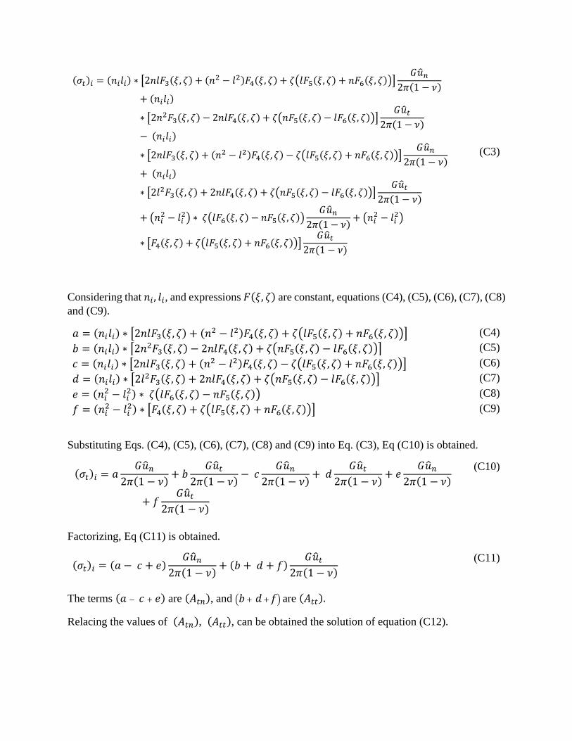
(𝜎𝑡)𝑖 = (𝑛𝑖𝑙𝑖) ∗ [2𝑛𝑙𝐹3(𝜉, 𝜁) + (𝑛2 − 𝑙2)𝐹4(𝜉, 𝜁) + 𝜁(𝑙𝐹5(𝜉, 𝜁) + 𝑛𝐹6(𝜉, 𝜁))]𝐺�̂�𝑛

2𝜋(1 − 𝜈)+ (𝑛𝑖𝑙𝑖)

∗ [2𝑛2𝐹3(𝜉, 𝜁) − 2𝑛𝑙𝐹4(𝜉, 𝜁) + 𝜁(𝑛𝐹5(𝜉, 𝜁) − 𝑙𝐹6(𝜉, 𝜁))]𝐺�̂�𝑡

2𝜋(1 − 𝜈)− (𝑛𝑖𝑙𝑖)

∗ [2𝑛𝑙𝐹3(𝜉, 𝜁) + (𝑛2 − 𝑙2)𝐹4(𝜉, 𝜁) − 𝜁(𝑙𝐹5(𝜉, 𝜁) + 𝑛𝐹6(𝜉, 𝜁))]𝐺�̂�𝑛

2𝜋(1 − 𝜈)+ (𝑛𝑖𝑙𝑖)

∗ [2𝑙2𝐹3(𝜉, 𝜁) + 2𝑛𝑙𝐹4(𝜉, 𝜁) + 𝜁(𝑛𝐹5(𝜉, 𝜁) − 𝑙𝐹6(𝜉, 𝜁))]𝐺�̂�𝑡

2𝜋(1 − 𝜈)

+ (𝑛𝑖2 − 𝑙𝑖

2) ∗ 𝜁(𝑙𝐹6(𝜉, 𝜁) − 𝑛𝐹5(𝜉, 𝜁))𝐺�̂�𝑛

2𝜋(1 − 𝜈)+ (𝑛𝑖

2 − 𝑙𝑖2)

∗ [𝐹4(𝜉, 𝜁) + 𝜁(𝑙𝐹5(𝜉, 𝜁) + 𝑛𝐹6(𝜉, 𝜁))]𝐺�̂�𝑡

2𝜋(1 − 𝜈)

(C3)

Considering that 𝑛𝑖 , 𝑙𝑖, and expressions 𝐹(𝜉, 𝜁) are constant, equations (C4), (C5), (C6), (C7), (C8)

and (C9).

𝑎 = (𝑛𝑖𝑙𝑖) ∗ [2𝑛𝑙𝐹3(𝜉, 𝜁) + (𝑛2 − 𝑙2)𝐹4(𝜉, 𝜁) + 𝜁(𝑙𝐹5(𝜉, 𝜁) + 𝑛𝐹6(𝜉, 𝜁))] (C4)

𝑏 = (𝑛𝑖𝑙𝑖) ∗ [2𝑛2𝐹3(𝜉, 𝜁) − 2𝑛𝑙𝐹4(𝜉, 𝜁) + 𝜁(𝑛𝐹5(𝜉, 𝜁) − 𝑙𝐹6(𝜉, 𝜁))] (C5)

𝑐 = (𝑛𝑖𝑙𝑖) ∗ [2𝑛𝑙𝐹3(𝜉, 𝜁) + (𝑛2 − 𝑙2)𝐹4(𝜉, 𝜁) − 𝜁(𝑙𝐹5(𝜉, 𝜁) + 𝑛𝐹6(𝜉, 𝜁))] (C6)

𝑑 = (𝑛𝑖𝑙𝑖) ∗ [2𝑙2𝐹3(𝜉, 𝜁) + 2𝑛𝑙𝐹4(𝜉, 𝜁) + 𝜁(𝑛𝐹5(𝜉, 𝜁) − 𝑙𝐹6(𝜉, 𝜁))] (C7)

𝑒 = (𝑛𝑖2 − 𝑙𝑖

2) ∗ 𝜁(𝑙𝐹6(𝜉, 𝜁) − 𝑛𝐹5(𝜉, 𝜁)) (C8)

𝑓 = (𝑛𝑖2 − 𝑙𝑖

2) ∗ [𝐹4(𝜉, 𝜁) + 𝜁(𝑙𝐹5(𝜉, 𝜁) + 𝑛𝐹6(𝜉, 𝜁))] (C9)

Substituting Eqs. (C4), (C5), (C6), (C7), (C8) and (C9) into Eq. (C3), Eq (C10) is obtained.

(𝜎𝑡)𝑖 = 𝑎𝐺�̂�𝑛

2𝜋(1 − 𝜈)+ 𝑏

𝐺�̂�𝑡

2𝜋(1 − 𝜈)− 𝑐

𝐺�̂�𝑛

2𝜋(1 − 𝜈)+ 𝑑

𝐺�̂�𝑡

2𝜋(1 − 𝜈)+ 𝑒

𝐺�̂�𝑛

2𝜋(1 − 𝜈)

+ 𝑓𝐺�̂�𝑡

2𝜋(1 − 𝜈)

(C10)

Factorizing, Eq (C11) is obtained.

(𝜎𝑡)𝑖 = (𝑎 − 𝑐 + 𝑒)𝐺�̂�𝑛

2𝜋(1 − 𝜈)+ (𝑏 + 𝑑 + 𝑓)

𝐺�̂�𝑡

2𝜋(1 − 𝜈)

(C11)

The terms (𝑎 − 𝑐 + 𝑒) are (𝐴𝑡𝑛), and (𝑏 + 𝑑 +𝑓) are (𝐴𝑡𝑡).

Relacing the values of (𝐴𝑡𝑛), (𝐴𝑡𝑡), can be obtained the solution of equation (C12).

(𝜎𝑡)𝑖 = ∑𝐺𝑖𝑗(𝐴𝑡𝑡)𝑖𝑗(�̂�𝑡)𝑗 + ∑𝐺𝑖𝑗(𝐴𝑡𝑛)𝑖𝑗(�̂�𝑛)𝑗

𝑁

𝑗=1

𝑁

𝑗=1

(C12)

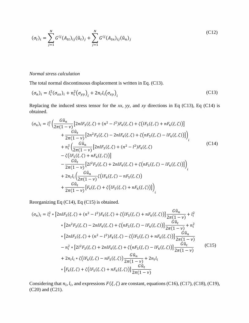
Normal stress calculation

The total normal discontinuous displacement is written in Eq. (C13).

(𝜎𝑛)𝑖 = 𝑙𝑖2(𝜎𝑥𝑥)𝑖 + 𝑛𝑖

2(𝜎𝑦𝑦)𝑖+ 2𝑛𝐼𝑙𝑖(𝜎𝑥𝑦)

𝑖

(C13)

Replacing the induced stress tensor for the xx, yy, and xy directions in Eq (C13), Eq (C14) is

obtained.

(𝜎𝑛)𝑖 = 𝑙𝑖2 (

𝐺�̂�𝑛

2𝜋(1 − 𝜈)[2𝑛𝑙𝐹3(𝜉, 𝜁) + (𝑛2 − 𝑙2)𝐹4(𝜉, 𝜁) + 𝜁(𝑙𝐹5(𝜉, 𝜁) + 𝑛𝐹6(𝜉, 𝜁))]

+𝐺�̂�𝑡

2𝜋(1 − 𝜈)[2𝑛2𝐹3(𝜉, 𝜁) − 2𝑛𝑙𝐹4(𝜉, 𝜁) + 𝜁(𝑛𝐹5(𝜉, 𝜁) − 𝑙𝐹6(𝜉, 𝜁))])

𝑖

+ 𝑛𝑖2 (

𝐺�̂�𝑛

2𝜋(1 − 𝜈)[2𝑛𝑙𝐹3(𝜉, 𝜁) + (𝑛2 − 𝑙2)𝐹4(𝜉, 𝜁)

− 𝜁(𝑙𝐹5(𝜉, 𝜁) + 𝑛𝐹6(𝜉, 𝜁))]

−𝐺�̂�𝑡

2𝜋(1 − 𝜈)[2𝑙2𝐹3(𝜉, 𝜁) + 2𝑛𝑙𝐹4(𝜉, 𝜁) + 𝜁(𝑛𝐹5(𝜉, 𝜁) − 𝑙𝐹6(𝜉, 𝜁))])

𝑖

+ 2𝑛𝐼𝑙𝑖 (𝐺�̂�𝑛

2𝜋(1 − 𝜈)𝜁(𝑙𝐹6(𝜉, 𝜁) − 𝑛𝐹5(𝜉, 𝜁))

+𝐺�̂�𝑡

2𝜋(1 − 𝜈)[𝐹4(𝜉, 𝜁) + 𝜁(𝑙𝐹5(𝜉, 𝜁) + 𝑛𝐹6(𝜉, 𝜁))])

𝑖

(C14)

Reorganizing Eq (C14), Eq (C15) is obtained.

(𝜎𝑛)𝑖 = 𝑙𝑖2 ∗ [2𝑛𝑙𝐹3(𝜉, 𝜁) + (𝑛2 − 𝑙2)𝐹4(𝜉, 𝜁) + 𝜁(𝑙𝐹5(𝜉, 𝜁) + 𝑛𝐹6(𝜉, 𝜁))]

𝐺�̂�𝑛

2𝜋(1 − 𝜈)+ 𝑙𝑖

2

∗ [2𝑛2𝐹3(𝜉, 𝜁) − 2𝑛𝑙𝐹4(𝜉, 𝜁) + 𝜁(𝑛𝐹5(𝜉, 𝜁) − 𝑙𝐹6(𝜉, 𝜁))]𝐺�̂�𝑡

2𝜋(1 − 𝜈)+ 𝑛𝑖

2

∗ [2𝑛𝑙𝐹3(𝜉, 𝜁) + (𝑛2 − 𝑙2)𝐹4(𝜉, 𝜁) − 𝜁(𝑙𝐹5(𝜉, 𝜁) + 𝑛𝐹6(𝜉, 𝜁))]𝐺�̂�𝑛

2𝜋(1 − 𝜈)

− 𝑛𝑖2 ∗ [2𝑙2𝐹3(𝜉, 𝜁) + 2𝑛𝑙𝐹4(𝜉, 𝜁) + 𝜁(𝑛𝐹5(𝜉, 𝜁) − 𝑙𝐹6(𝜉, 𝜁))]

𝐺�̂�𝑡

2𝜋(1 − 𝜈)

+ 2𝑛𝐼𝑙𝑖 ∗ 𝜁(𝑙𝐹6(𝜉, 𝜁) − 𝑛𝐹5(𝜉, 𝜁))𝐺�̂�𝑛

2𝜋(1 − 𝜈)+ 2𝑛𝐼𝑙𝑖

∗ [𝐹4(𝜉, 𝜁) + 𝜁(𝑙𝐹5(𝜉, 𝜁) + 𝑛𝐹6(𝜉, 𝜁))]𝐺�̂�𝑡

2𝜋(1 − 𝜈)

(C15)

Considering that 𝑛𝑖 , 𝑙𝑖, and expressions 𝐹(𝜉, 𝜁) are constant, equations (C16), (C17), (C18), (C19),

(C20) and (C21).

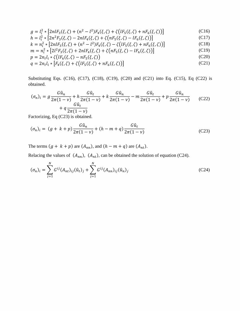
𝑔 = 𝑙𝑖2 ∗ [2𝑛𝑙𝐹3(𝜉, 𝜁) + (𝑛2 − 𝑙2)𝐹4(𝜉, 𝜁) + 𝜁(𝑙𝐹5(𝜉, 𝜁) + 𝑛𝐹6(𝜉, 𝜁))] (C16)

ℎ = 𝑙𝑖2 ∗ [2𝑛2𝐹3(𝜉, 𝜁) − 2𝑛𝑙𝐹4(𝜉, 𝜁) + 𝜁(𝑛𝐹5(𝜉, 𝜁) − 𝑙𝐹6(𝜉, 𝜁))] (C17)

𝑘 = 𝑛𝑖2 ∗ [2𝑛𝑙𝐹3(𝜉, 𝜁) + (𝑛2 − 𝑙2)𝐹4(𝜉, 𝜁) − 𝜁(𝑙𝐹5(𝜉, 𝜁) + 𝑛𝐹6(𝜉, 𝜁))] (C18)

𝑚 = 𝑛𝑖2 ∗ [2𝑙2𝐹3(𝜉, 𝜁) + 2𝑛𝑙𝐹4(𝜉, 𝜁) + 𝜁(𝑛𝐹5(𝜉, 𝜁) − 𝑙𝐹6(𝜉, 𝜁))] (C19)

𝑝 = 2𝑛𝐼𝑙𝑖 ∗ 𝜁(𝑙𝐹6(𝜉, 𝜁) − 𝑛𝐹5(𝜉, 𝜁)) (C20)

𝑞 = 2𝑛𝐼𝑙𝑖 ∗ [𝐹4(𝜉, 𝜁) + 𝜁(𝑙𝐹5(𝜉, 𝜁) + 𝑛𝐹6(𝜉, 𝜁))] (C21)

Substituting Eqs. (C16), (C17), (C18), (C19), (C20) and (C21) into Eq. (C15), Eq (C22) is

obtained.

(𝜎𝑛)𝑖 = 𝑔𝐺�̂�𝑛

2𝜋(1 − 𝜈)+ ℎ

𝐺�̂�𝑡

2𝜋(1 − 𝜈)+ 𝑘

𝐺�̂�𝑛

2𝜋(1 − 𝜈)− 𝑚

𝐺�̂�𝑡

2𝜋(1 − 𝜈)+ 𝑝

𝐺�̂�𝑛

2𝜋(1 − 𝜈)

+ 𝑞𝐺�̂�𝑡

2𝜋(1 − 𝜈)

(C22)

Factorizing, Eq (C23) is obtained.

(𝜎𝑛)𝑖 = (𝑔 + 𝑘 + 𝑝)𝐺�̂�𝑛

2𝜋(1 − 𝜈)+ (ℎ − 𝑚 + 𝑞)

𝐺�̂�𝑡

2𝜋(1 − 𝜈)

(C23)

The terms (𝑔 + 𝑘 + 𝑝) are (𝐴𝑛𝑛), and (ℎ − 𝑚 + 𝑞) are (𝐴𝑛𝑡).

Relacing the values of (𝐴𝑛𝑛), (𝐴𝑛𝑡), can be obtained the solution of equation (C24).

(𝜎𝑛)𝑖 = ∑𝐺𝑖𝑗(𝐴𝑛𝑡)𝑖𝑗(�̂�𝑡)𝑗 + ∑𝐺𝑖𝑗(𝐴𝑛𝑛)𝑖𝑗(�̂�𝑛)𝑗

𝑁

𝑗=1

𝑁

𝑗=1

(C24)