Simultaneous Localization, Mapping and Moving Object … · Simultaneous Localization, Mapping and...

Simultaneous Localization, Mapping andMoving Object Tracking

Chieh-Chih WangDepartment of Computer Science and Information Engineering and

Graduate Institute of Networking and MultimediaNational Taiwan University

Taipei 106, [email protected]

Charles Thorpe, Martial HebertThe Robotics Institute

Carnegie Mellon UniversityPittsburgh, PA 15213, USA

[email protected], [email protected]

Sebastian ThrunThe AI group

Stanford UniversityStanford, CA 94305, [email protected]

Hugh Durrant-WhyteThe ARC Centre of Excellence for Autonomous Systems

The University of SydneyNSW 2006, Australia

[email protected]

Abstract

Simultaneous localization, mapping and moving object tracking (SLAMMOT)involves both simultaneous localization and mapping (SLAM) in dynamic en-vironments and detecting and tracking these dynamic objects. In this paper,we establish a mathematical framework to integrate SLAM and moving ob-ject tracking. We describe two solutions: SLAM with generalized objects, andSLAM with detection and tracking of moving objects (DATMO). SLAM withgeneralized objects calculates a joint posterior over all generalized objects andthe robot. Such an approach is similar to existing SLAM algorithms, but withadditional structure to allow for motion modeling of generalized objects. Un-fortunately, it is computationally demanding and generally infeasible. SLAMwith DATMO decomposes the estimation problem into two separate estima-tors. By maintaining separate posteriors for stationary objects and movingobjects, the resulting estimation problems are much lower dimensional thenSLAM with generalized objects. Both SLAM and moving object trackingfrom a moving vehicle in crowded urban areas are daunting tasks. Based onthe SLAM with DATMO framework, we propose practical algorithms whichdeal with issues of perception modeling, data association, and moving object

detection. The implementation of SLAM with DATMO was demonstrated us-ing data collected from the CMU Navlab11 vehicle at high speeds in crowdedurban environments. Ample experimental results shows the feasibility of theproposed theory and algorithms.

1 Introduction

Establishing the spatial and temporal relationships among a robot, stationary objects andmoving objects in a scene serves as a basis for scene understanding. Localization is theprocess of establishing the spatial relationships between the robot and stationary objects,mapping is the process of establishing the spatial relationships among stationary objects,and moving object tracking is the process of establishing the spatial and temporal relation-ships between moving objects and the robot or between moving and stationary objects.Localization, mapping and moving object tracking are difficult because of uncertainty andunobservable states in the real world. Perception sensors such as cameras, radar and laserrange finders, and motion sensors such as odometry and inertial measurement units are noisy.The intentions, or control inputs, of the moving objects are unobservable without using extrasensors mounted on the moving objects.

Over the last decade, the simultaneous localization and mapping (SLAM) problem has at-tracted immense attention in the mobile robotics and artificial intelligence literature (Smithand Cheeseman, 1986; Thrun, 2002). SLAM involves simultaneously estimating locations ofnewly perceived landmarks and the location of the robot itself while incrementally buildinga map. The moving object tracking problem has also been extensively studied for severaldecades (Bar-Shalom and Li, 1988; Blackman and Popoli, 1999). Moving object trackinginvolves both state inference and motion model learning. In most applications, SLAM andmoving object tracking are considered in isolation. In the SLAM problem, information as-sociated with stationary objects are positive; moving objects are negative, which degradesthe performance. Conversely, measurements belonging to moving objects are positive in themoving object tracking problem; stationary objects are considered background and filteredout. In (Wang and Thorpe, 2002), we pointed out that SLAM and moving object trackingare mutually beneficial. Both stationary objects and moving objects are positive informationto scene understanding. In (Wang et al., 2003b), we established a mathematical frameworkto integrate SLAM and moving object tracking, which provides a solid basis for understand-ing and solving the whole problem, simultaneous localization, mapping and moving objecttracking, or SLAMMOT.

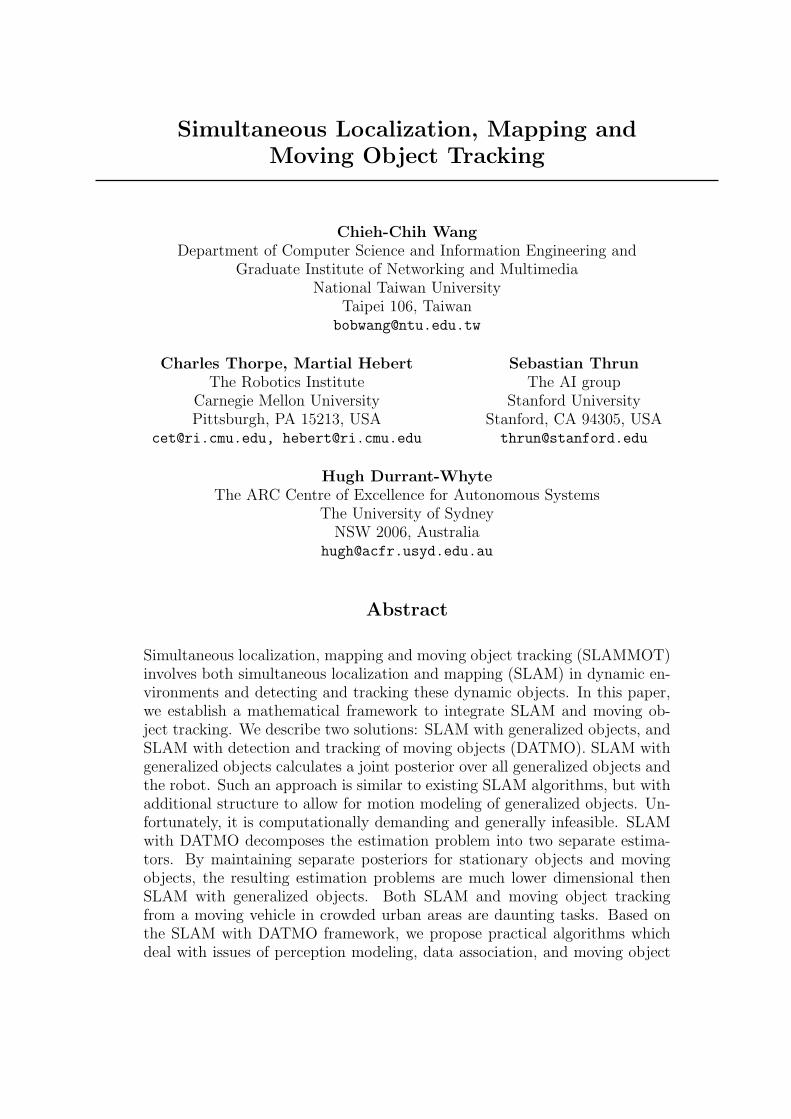
It is believed by many that a solution to the SLAM problem will open up a vast range of po-tential applications for autonomous robots (Thorpe and Durrant-Whyte, 2001; Christensen,2002). We believe that a solution to the SLAMMOT problem will expand the potential forrobotic applications still further, especially in applications which are in close proximity tohuman beings. Robots will be able to work not only for people but also with people. Figure1 illustrates a commercial application, safe driving, which motivates the work in this paper.

To improve driving safety and prevent traffic injuries caused by human factors such as

Figure 1: Robotics for safe driving. Localization, mapping, and moving object tracking arecritical to driving assistance and autonomous driving.

speeding and distraction, methods for understanding the surroundings of the vehicle arecritical. We believe that being able to detect and track every stationary object and everymoving object, to reason about the dynamic traffic scene, to detect and predict criticalsituations, and to warn and assist drivers in advance, is essential to prevent these kinds ofaccidents.

To detect and track moving objects using sensors mounted on a moving ground vehicle athigh speeds, a precise localization system is essential. It is known that GPS and DGPS oftenfails in urban areas because of ”urban canyon” effects, and good inertial measurement units(IMU) are very expensive.

If we have a stationary object map in advance, map-based localization techniques (Olson,2000)(Fox et al., 1999)(Dellaert et al., 1999) can be used to increase the accuracy of thepose estimate. Unfortunately, it is difficult to build a usable stationary object map becauseof temporary stationary objects such as parked cars. Stationary object maps of the samescene built at different times could still be different, which means that online map buildingis required to update the current stationary object map.

SLAM allows robots to operate in an unknown environment, to incrementally build a mapof this environment and to simultaneously use this map to localize the robots themselves.However, we have observed (Wang and Thorpe, 2002) that SLAM can perform badly incrowded urban environments because the static environment assumption may be violated;moving objects have to be detected and filtered out.

Even with precise localization, it is not easy to solve the moving object tracking problemin crowded urban environments because of the wide variety of targets (Wang et al., 2003a).When cameras are used to detect moving objects, appearance-based approaches are widelyused and moving objects should be detected no matter whether they are moving or not. Iflaser scanners are used, feature-based approaches are usually the preferred solution. Bothappearance-based and feature-based methods rely on prior knowledge of the targets. In urbanareas, there are many kinds of moving objects such as pedestrians, bicycles, motorcycles,

cars, buses, trucks and trailers. Velocities range from under 5 mph (such as a pedestrian’smovement) to 50 mph. When using laser scanners, the features of moving objects canchange significantly from scan to scan. As a result, it is often difficult to define features orappearances for detecting specific objects.

Both SLAM and moving object tracking have been solved and implemented successfully inisolation. However, when driving in crowded urban environments composed of stationaryand moving objects, neither of them is sufficient in isolation. The SLAMMOT problemaims to tackle the SLAM problem and the moving object tracking problem concurrently.SLAM provides more accurate pose estimates together with a surrounding map. Movingobjects can be detected using the surrounding map without recourse to predefined featuresor appearances. Tracking may then be performed reliably with accurate robot pose estimates.SLAM can be more accurate because moving objects are filtered out of the SLAM processthanks to the moving object location prediction. SLAM and moving object tracking aremutually beneficial. Integrating SLAM and moving object tracking would satisfy both thesafety and navigation demands of safe driving. It would provide a better estimate of therobot’s location and information of the dynamic environments, which are critical to drivingassistance and autonomous driving.

In this paper we first establish the mathematical framework for performing SLAMMOT.We will describe two algorithms, SLAM with generalized objects and SLAM with detectionand tracking of moving object (DATMO). SLAM with DATMO decomposes the estimationproblem of SLAMMOT into two separate estimators. By maintaining separate posteriorsfor stationary objects and moving objects, the resulting estimation problems are much lowerdimensional than SLAM with generalized objects. This makes it feasible to update bothfilters in real-time. In this paper, SLAM with DATMO is applied and implemented.

There are significant practical issues to be considered in bridging the gap between the pre-sented theory and its applications to real problems such as driving safely at high speedsin crowded urban areas. These issues arise from a number of implicit assumptions in per-ception modeling and data association. When using more accurate sensors, these problemare easier to solve, and inference and learning of the SLAM with DATMO problem becomemore practical and tractable. Therefore, we mainly focus on issues of using active rangingsensors. SICK laser scanners (see Figure 2) are used and studied in this work. Data sets(Wang et al., 2004) collected from the Navlab11 testbed are used to verify the theory andalgorithms. Visual images from an omni-directional camera and a tri-camera system areonly used for visualization. Sensors carrying global localization information such as GPSand DGPS are not used.

The remainder of this paper is organized as follows. In Section 2, related research is ad-dressed. The formulations and algorithms of SLAM and moving object tracking are brieflyreviewed in Section 3. In Section 4, we introduce SLAM with generalized object and SLAMwith DATMO and discuss some of important issues such as motion mode learning, com-putational complexity and interaction. The proposed algorithms which deal with issues ofperception modeling, data association and moving object detection are described in Section5, Section 6 and Section 7, respectively. Experimental results which demonstrated the fea-sibility of the proposed theory and algorithms are in Section 8. Finally, the conclusion and

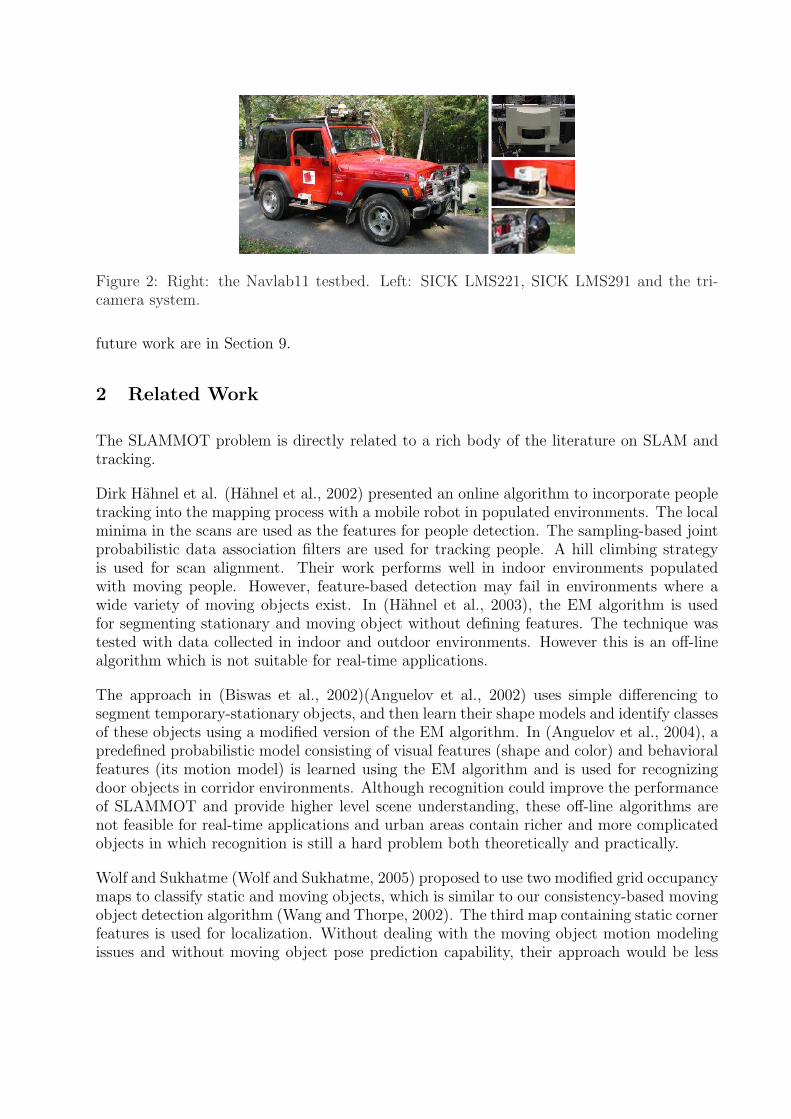
Figure 2: Right: the Navlab11 testbed. Left: SICK LMS221, SICK LMS291 and the tri-camera system.

future work are in Section 9.

2 Related Work

The SLAMMOT problem is directly related to a rich body of the literature on SLAM andtracking.

Dirk Hahnel et al. (Hahnel et al., 2002) presented an online algorithm to incorporate peopletracking into the mapping process with a mobile robot in populated environments. The localminima in the scans are used as the features for people detection. The sampling-based jointprobabilistic data association filters are used for tracking people. A hill climbing strategyis used for scan alignment. Their work performs well in indoor environments populatedwith moving people. However, feature-based detection may fail in environments where awide variety of moving objects exist. In (Hahnel et al., 2003), the EM algorithm is usedfor segmenting stationary and moving object without defining features. The technique wastested with data collected in indoor and outdoor environments. However this is an off-linealgorithm which is not suitable for real-time applications.

The approach in (Biswas et al., 2002)(Anguelov et al., 2002) uses simple differencing tosegment temporary-stationary objects, and then learn their shape models and identify classesof these objects using a modified version of the EM algorithm. In (Anguelov et al., 2004), apredefined probabilistic model consisting of visual features (shape and color) and behavioralfeatures (its motion model) is learned using the EM algorithm and is used for recognizingdoor objects in corridor environments. Although recognition could improve the performanceof SLAMMOT and provide higher level scene understanding, these off-line algorithms arenot feasible for real-time applications and urban areas contain richer and more complicatedobjects in which recognition is still a hard problem both theoretically and practically.

Wolf and Sukhatme (Wolf and Sukhatme, 2005) proposed to use two modified grid occupancymaps to classify static and moving objects, which is similar to our consistency-based movingobject detection algorithm (Wang and Thorpe, 2002). The third map containing static cornerfeatures is used for localization. Without dealing with the moving object motion modelingissues and without moving object pose prediction capability, their approach would be less

robust than the proposed approach in this paper. Montesano et al. (Montesano et al., 2005)integrated the SLAMMOT and planning processes to improve robot navigation in dynamicenvironments as well as extended our SLAM with DATMO algorithm to jointly solve themoving and stationary object classification problem in an indoor environment. In this paper,the proposed theory of SLAM with generalized objects and SLAM with DATMO addressmore related issues such as interaction, and the proposed algorithms are demonstrated froma ground vehicle at high speeds in crowded urban environments.

The SLAMMOT problem is also closely related to the computer vision literature. Demird-jian and Horaud (Demirdjian and Horaud, 2000) addressed the problem of segmenting theobserved scene into static and moving objects from a moving stereo rig. They apply a ro-bust method, random sample consensus (RANSAC), for filtering out the moving objects andoutliers. Although the RANSAC method can tolerate up to 50% outliers, the percentage ofmoving objects is often more than stationary objects and degeneracies exist in our applica-tions. With measurements from motion sensors, stationary and moving object maps, andprecise localization, our moving object detectors perform reliably in real-time.

Recently, the problem of recovery non-rigid shape and motion of dynamic scenes from amoving camera has attracted immense attention in the computer vision literature. The ideasbased on the factorization techniques and the shape basis representation are presented in(Bregler et al., 2000)(Brand, 2001)(Torresani et al., 2001)(Xiao et al., 2004) where differentconstraints are used for finding the solution. Theoretically, all of these batch approaches areinappropriate to use in real-time. Practically, these methods are computational demandingand many difficulties such as occlusions, motion blur and lighting conditions remain to bedeveloped.

3 Foundations

SLAM assumes that the surrounding environment is static, containing only stationary ob-jects. The inputs of the SLAM process are measurements from perception sensors such aslaser scanners and cameras, and measurements from motion sensors such as odometry andinertial measurement units. The outputs of the SLAM process are the robot pose and astationary object map (see Figure 3.a). Given that the sensor platform is stationary or thata precise pose estimate is available, the inputs of the moving object tracking problem areperception measurements and the outputs are locations of moving objects and their motionmodes (see Figure 3.b). The SLAMMOT problem can also be treated as a process with-out the static environment assumption. The inputs of this process are the same as for theSLAM process, but the outputs are both robot pose and map, together with the locationsand motion modes of the moving objects (see Figure 3.c).

Leaving aside perception and data association, the key issue in SLAM is the computationalcomplexity of updating and maintaining the map, and the key issue of the moving objecttracking problem is the computational complexity of motion modelling. As SLAMMOTinherits the complexity issue from SLAM and the motion modelling issue from moving objecttracking, the SLAMMOT problem is both an inference problem and a learning problem.

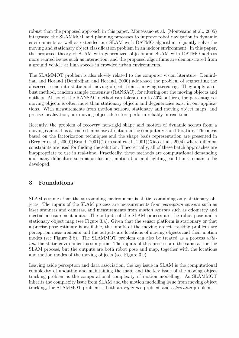
(a) the simultaneous localization and mapping (SLAM) process

(b) the moving object tracking (MOT) process

(c) the simultaneous localization, mapping and moving object tracking (SLAMMOT)process

Figure 3: The SLAM process, the MOT process and the SLAMMOT process. Z denotes theperception measurements, U denotes the motion measurements, x is the true robot state, Mdenotes the locations of the stationary objects, O denotes the states of the moving objectsand S denotes the motion modes of the moving objects.

In this section we briefly introduce SLAM and moving object tracking.

3.1 Notation

Let k denote the discrete time index, uk the vector describing a motion measurement fromtime k − 1 to time k, zk a measurement from perception sensors such as laser scanners attime k, xk the state vector describing the true pose of the robot at time k, and Mk the mapcontain l landmarks, m1,m2, . . . ,ml, at time k. In addition, we define the following sets:

Xk4= {x0, x1, . . . , xk} (1)

Zk4= {z0, z1, . . . , zk} (2)

Uk4= {u1, u2, . . . , uk} (3)

3.2 Simultaneous Localization and Mapping

The SLAM problem is to determine the robot poses xk and the stationary object map Mk

given perception measurements Zk and motion measurement Uk.

The formula for sequential SLAM can be expressed as

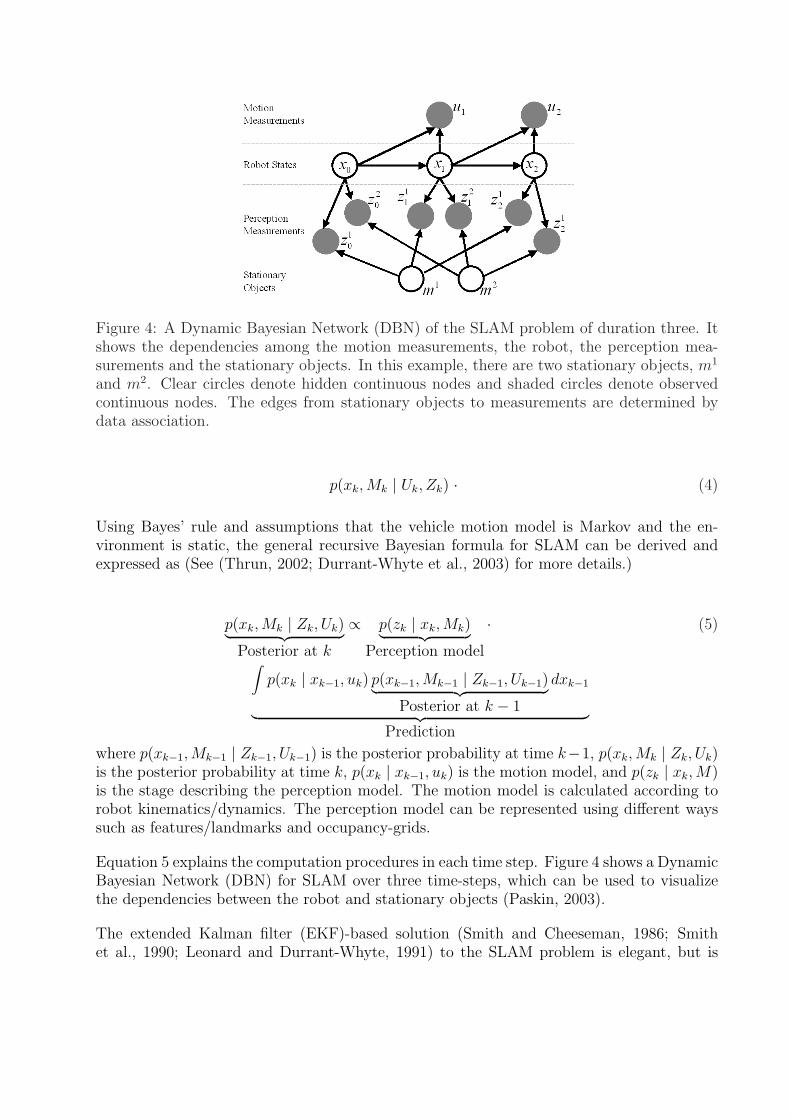
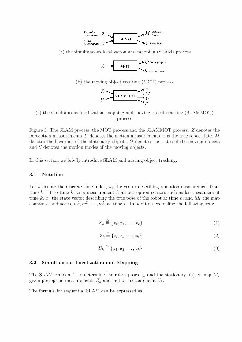
Figure 4: A Dynamic Bayesian Network (DBN) of the SLAM problem of duration three. Itshows the dependencies among the motion measurements, the robot, the perception mea-surements and the stationary objects. In this example, there are two stationary objects, m1

and m2. Clear circles denote hidden continuous nodes and shaded circles denote observedcontinuous nodes. The edges from stationary objects to measurements are determined bydata association.

p(xk,Mk | Uk, Zk) · (4)

Using Bayes’ rule and assumptions that the vehicle motion model is Markov and the en-vironment is static, the general recursive Bayesian formula for SLAM can be derived andexpressed as (See (Thrun, 2002; Durrant-Whyte et al., 2003) for more details.)

p(xk,Mk | Zk, Uk)︸︷︷︸Posterior at k

∝ p(zk | xk,Mk)︸︷︷︸Perception model

· (5)

∫p(xk | xk−1, uk) p(xk−1,Mk−1 | Zk−1, Uk−1)︸︷︷︸

Posterior at k − 1

dxk−1

︸︷︷︸Prediction

where p(xk−1,Mk−1 | Zk−1, Uk−1) is the posterior probability at time k−1, p(xk,Mk | Zk, Uk)is the posterior probability at time k, p(xk | xk−1, uk) is the motion model, and p(zk | xk,M)is the stage describing the perception model. The motion model is calculated according torobot kinematics/dynamics. The perception model can be represented using different wayssuch as features/landmarks and occupancy-grids.

Equation 5 explains the computation procedures in each time step. Figure 4 shows a DynamicBayesian Network (DBN) for SLAM over three time-steps, which can be used to visualizethe dependencies between the robot and stationary objects (Paskin, 2003).

The extended Kalman filter (EKF)-based solution (Smith and Cheeseman, 1986; Smithet al., 1990; Leonard and Durrant-Whyte, 1991) to the SLAM problem is elegant, but is

computational complex. Approaches using approximate inference, using exact inference ontractable approximations of the true model, and using approximate inference on an ap-proximate model have been proposed (Paskin, 2003; Thrun et al., 2002; Bosse et al., 2003;Guivant and Nebot, 2001; Leonard and Feder, 1999; Montemerlo, 2003). Paskin (Paskin,2003) included an excellent comparison of these techniques.

3.3 Moving Object Tracking

Just as with SLAM, moving object tracking can be formulated with Bayesian approachessuch as Kalman filtering. Moving object tracking is generally easier than SLAM since onlythe moving object pose is maintained and updated. However, as motion models of movingobjects are often time-varying and not known with accuracy, moving object tracking is moredifficult than SLAM in terms of online motion model learning.

The general recursive probabilistic formula for moving object tracking can be expressed as

p(ok, sk | Zk) (6)

where ok is the true state of a moving object at time k, and sk is the true motion mode ofthe moving object at time k, and Zk is the perception measurement set leading up to timek. The robot (sensor platform) is assumed to be stationary for the sake of simplicity.

Using Bayes’ rule, Equation 6 can be rewritten as

p(ok, sk | Zk) = p(ok | sk, Zk)︸︷︷︸State inference

· p(sk | Zk)︸︷︷︸Mode learning

(7)

which indicates that the moving object tracking problem can be solved in two stages: thefirst stage is the mode learning stage p(sk | Zk), and the second stage is the state inferencestage p(ok | sk, Zk).

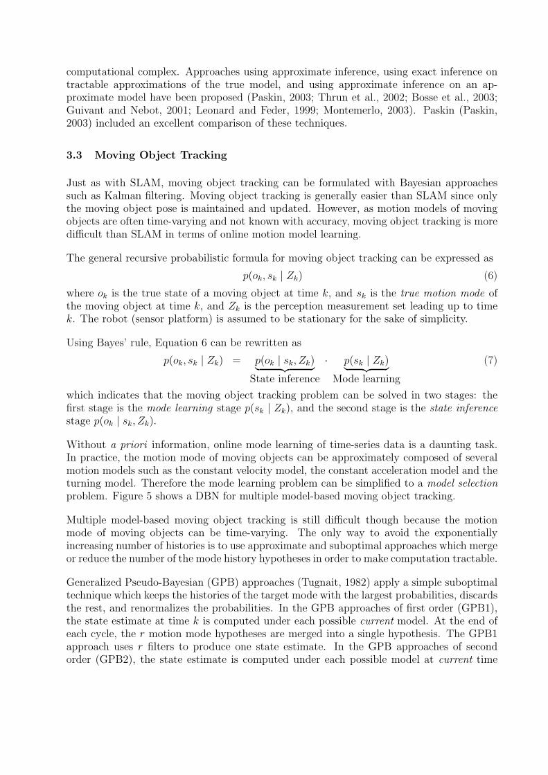
Without a priori information, online mode learning of time-series data is a daunting task.In practice, the motion mode of moving objects can be approximately composed of severalmotion models such as the constant velocity model, the constant acceleration model and theturning model. Therefore the mode learning problem can be simplified to a model selectionproblem. Figure 5 shows a DBN for multiple model-based moving object tracking.

Multiple model-based moving object tracking is still difficult though because the motionmode of moving objects can be time-varying. The only way to avoid the exponentiallyincreasing number of histories is to use approximate and suboptimal approaches which mergeor reduce the number of the mode history hypotheses in order to make computation tractable.

Generalized Pseudo-Bayesian (GPB) approaches (Tugnait, 1982) apply a simple suboptimaltechnique which keeps the histories of the target mode with the largest probabilities, discardsthe rest, and renormalizes the probabilities. In the GPB approaches of first order (GPB1),the state estimate at time k is computed under each possible current model. At the end ofeach cycle, the r motion mode hypotheses are merged into a single hypothesis. The GPB1approach uses r filters to produce one state estimate. In the GPB approaches of secondorder (GPB2), the state estimate is computed under each possible model at current time

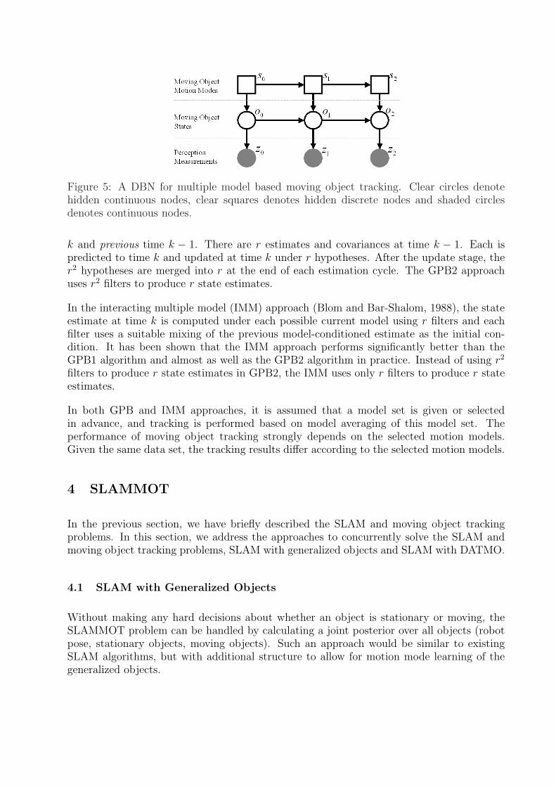
Figure 5: A DBN for multiple model based moving object tracking. Clear circles denotehidden continuous nodes, clear squares denotes hidden discrete nodes and shaded circlesdenotes continuous nodes.

k and previous time k − 1. There are r estimates and covariances at time k − 1. Each ispredicted to time k and updated at time k under r hypotheses. After the update stage, ther2 hypotheses are merged into r at the end of each estimation cycle. The GPB2 approachuses r2 filters to produce r state estimates.

In the interacting multiple model (IMM) approach (Blom and Bar-Shalom, 1988), the stateestimate at time k is computed under each possible current model using r filters and eachfilter uses a suitable mixing of the previous model-conditioned estimate as the initial con-dition. It has been shown that the IMM approach performs significantly better than theGPB1 algorithm and almost as well as the GPB2 algorithm in practice. Instead of using r2

filters to produce r state estimates in GPB2, the IMM uses only r filters to produce r stateestimates.

In both GPB and IMM approaches, it is assumed that a model set is given or selectedin advance, and tracking is performed based on model averaging of this model set. Theperformance of moving object tracking strongly depends on the selected motion models.Given the same data set, the tracking results differ according to the selected motion models.

4 SLAMMOT

In the previous section, we have briefly described the SLAM and moving object trackingproblems. In this section, we address the approaches to concurrently solve the SLAM andmoving object tracking problems, SLAM with generalized objects and SLAM with DATMO.

4.1 SLAM with Generalized Objects

Without making any hard decisions about whether an object is stationary or moving, theSLAMMOT problem can be handled by calculating a joint posterior over all objects (robotpose, stationary objects, moving objects). Such an approach would be similar to existingSLAM algorithms, but with additional structure to allow for motion mode learning of thegeneralized objects.

4.1.1 Bayesian Formulation

The formalization of SLAM with generalized objects is straightforward. First we define thatthe generalized object is a hybrid state consisting of the state and the motion mode.

yik4= {yi

k, sik} and Yk

4= {y1

k,y2k, . . . ,y

lk} (8)

where yk is the true state of the generalized object, sk is the true motion mode of thegeneralized object and l is the number of generalized objects. Note that generalized objectscan be moving, stationary, or move-stop-move entities. We then use this hybrid variable Yto replace the variable M in Equation 5 and the general recursive probabilistic formula ofSLAM with generalized objects can be expressed as:

p(xk,Yk | Uk, Zk) (9)

Using Bayes’ rules and assumptions that the motion models of the robot and generalizedobjects are Markov and there is no interaction among the robot and generalized objects, thegeneral recursive Bayesian formula for SLAM with generalized objects can be derived andexpresses as: (See Appendix A for derivation.)

p(xk,Yk | Uk, Zk)︸︷︷︸Posterior at k

∝ p(zk | xk,Yk)︸︷︷︸Update

∫ ∫p(xk | xk−1, uk)︸︷︷︸Robot predict

p(Yk | Yk−1)︸︷︷︸generalized objs

· p(xk−1,Yk−1 | Zk−1, Uk−1)︸︷︷︸Posterior at k − 1

dxk−1 dYk−1 (10)

where p(xk−1,Yk−1 | Zk−1, Uk−1) is the posterior probability at time k−1, p(xk,Yk | Uk, Zk)is the posterior probability at time k. In the prediction stage p(xk | xk−1, uk)p(Yk | Yk−1),the states of the robot state and generalized objects are predicted independently with theno interaction assumption. In the update stage p(zk | xk,Yk), the states of the robot andgeneralized objects as well as their motion models are updated concurrently. In the casesthat interactions among the robot and generalized objects exist, the formula for SLAM withgeneralized objects is also shown in Appendix A.

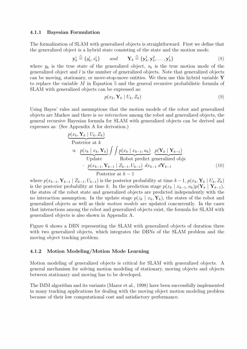
Figure 6 shows a DBN representing the SLAM with generalized objects of duration threewith two generalized objects, which integrates the DBNs of the SLAM problem and themoving object tracking problem.

4.1.2 Motion Modeling/Motion Mode Learning

Motion modeling of generalized objects is critical for SLAM with generalized objects. Ageneral mechanism for solving motion modeling of stationary, moving objects and objectsbetween stationary and moving has to be developed.

The IMM algorithm and its variants (Mazor et al., 1998) have been successfully implementedin many tracking applications for dealing with the moving object motion modeling problembecause of their low computational cost and satisfactory performance.

Figure 6: A DBN for SLAM with Generalized Objects. It is an integration of the DBN ofthe SLAM problem (Figure 4) and the DBN of the moving object tracking problem (Figure5).

Adding a stationary motion model to the motion model set with the same IMM algorithmfor dealing with move-stop-move maneuvers was suggested in (Kirubarajan and Bar-Shalom,2000; Coraluppi et al., 2000; Coraluppi and Carthel, 2001). However, as observed in (Sheaet al., 2000; Coraluppi and Carthel, 2001), all of the estimates tend to degrade when the stop(stationary motion) model is added to the model set and mixed with other moving motionmodels. This topic is beyond the scope intended by this paper. We provide a theoreticalexplanation of this phenomenon and a practical solution, move-stop hypothesis tracking, inChapter 4 of (Wang, 2004).

4.1.3 Highly Maneuverable Objects

The framework of SLAM with generalized objects indicates that measurements belongingto moving objects contribute to localization and mapping as well as stationary objects.Nevertheless, highly maneuverable objects are difficult to track and often unpredictablein practice. Including them in localization and mapping would have a minimal effect onlocalization accuracy.

4.1.4 Computational Complexity

In the SLAM literature, it is known that a key bottleneck of the Kalman filter solution is itscomputational complexity. Because it explicitly represents correlations of all pairs amongthe robot and stationary objects, both the computation time and memory requirement scalequadratically with the number of stationary objects in the map. This computational burdenrestricts applications to those in which the map can have no more than a few hundredstationary objects. Recently, this problem has been subject to intense research.

In the framework of SLAM with generalized objects, the robot, stationary and moving objectsare generally correlated through the convolution process in the prediction and update stages.Although the formulation of SLAM with generalized objects is elegant, it is clear that SLAMwith generalized objects is much more computationally demanding than SLAM due to therequired motion modeling of all generalized objects at all time steps. Given that real-timemotion modeling of generalized objects and interaction among moving and stationary objectsare still open questions, the computational complexity of SLAM with generalized objects isnot further analyzed.

4.2 SLAM with DATMO

SLAM with generalized objects is similar to existing SLAM algorithms, but with additionalstructure to allow for motion modelling of generalized objects. Unfortunately, it is com-putationally demanding and generally infeasible. Consequently, in this section we providethe second approach, SLAM with DATMO, in which the estimation problem is decomposedinto two separate estimators. By maintaining separate posteriors for stationary objects andmoving objects, the resulting estimation problem is of lower dimension than SLAM withgeneralized objects, making it feasible to update both filters in real time.

4.2.1 Bayesian Formulation

Let ok denote the true hybrid state of the moving object at time k.

oik4= {oi

k, sik} (11)

where ok is the true state of the moving object, sk is the true motion mode of the movingobject.

In SLAM with DATMO, three assumption are made to simply the computation of SLAMwith generalized objects. One of the key assumptions is that measurements can be decom-posed into measurement of stationary and moving objects. This implies that objects can beclassified as stationary or moving in which the general SLAM with DATMO problem can beposed as computing the posterior

p(xk,Ok,Mk | Zk, Uk) (12)

where the variable Ok = {o1k,o

2k, . . . ,o

nk} denotes the true hybrid states of the moving

objects, of which there are n in the world at time k, and the variable Mk = {m1k,m

2k, . . . ,m

qk}

denotes the true locations of the stationary objects, of which there are q in the world at timek. The second assumption is that when estimating the posterior over the stationary objectmap and the robot pose, the measurements of moving objects carry no information aboutstationary landmarks and the robot pose, neither do their hybrid states Ok. The thirdassumption is that there is no interaction among the robot and the moving objects. Therobot and moving objects move independently of each other.

Using Bayes’ rules and the assumptions addressed in Appendix B, the general recursiveBayesian formula for SLAM with DATMO can be derived and expresses as: (See Appendix

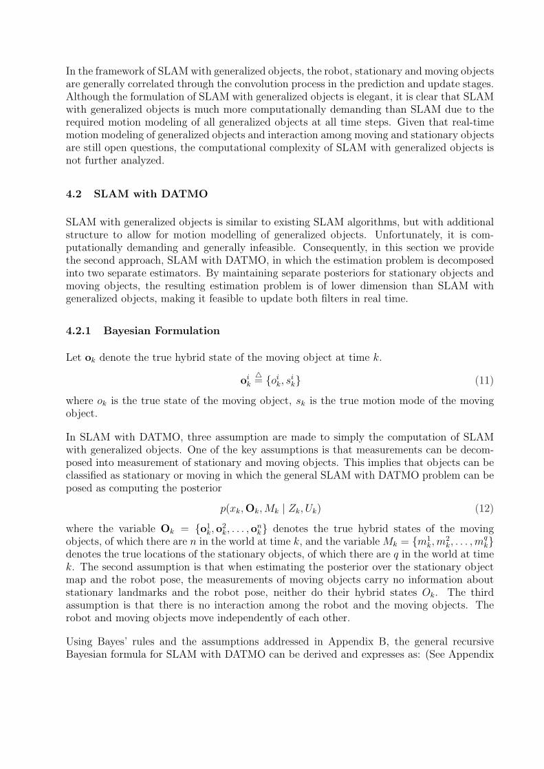
Figure 7: A Dynamic Bayesian Network of the SLAM with DATMO problem of durationthree with one moving object and one stationary object.

B for derivation.)

p(xk,Ok,Mk | Zk, Uk) (13)

∝ p(zok | xk,Ok) p(Ok | Zo

k−1, Uk)︸︷︷︸DATMO

· p(zmk | xk,Mk) p(xk,Mk | Zm

k−1, Uk)︸︷︷︸SLAM

= p(zok | Ok, xk)︸︷︷︸

DATMO Update

·∫

p(Ok | Ok−1) p(Ok−1 | Zok−1, Uk−1) dOk−1

︸︷︷︸DATMO Prediction

· p(zmk | Mk, xk)︸︷︷︸

SLAM Update

·∫

p(xk | uk, xk−1) p(xk−1, Mk−1 | Zmk−1, Uk−1) dxk−1

︸︷︷︸SLAM Prediction

where zmk and zo

k denote measurements of stationary and moving objects, respectively. Equa-tion 13 shows how the SLAMMOT problem is decomposed into separate posteriors for movingand stationary objects. It also indicates that DATMO should take account of the uncertaintyin the pose estimate of the robot because perception measurements are directly from therobot.

Figure 7 shows a DBN representing three time steps of an example SLAM with DATMOproblem with one moving object and one stationary object.

4.2.2 Detection/Classification

Correctly detecting or classifying moving and stationary objects is essential for successfullyimplementing SLAM with DATMO. In the tracking literature, a number of approaches havebeen proposed for detecting moving objects, which can be classified into two categories: withand without the use of thresholding. Gish and Mucci (Gish and Mucci, 1987) proposed anapproach that detection and tracking occur simultaneously without using a threshold. Thisapproach is called track before detect (TBD), although detection and tracking are performedsimultaneously. However, the high computational requirements of this approach make theimplementation infeasible. Arnold et al. (Arnold et al., 1993) showed that integrating TBDwith a dynamic programming algorithm provides an efficient solution for detection withoutthresholding, which could be a solution for implementing SLAM with generalized objectspractically. In Section 7, we will present two reliable approaches for detecting or classifyingmoving and stationary objects from laser scanners.

4.3 Interaction

Thus far, we have described the SLAMMOT problem which involves both SLAM in dynamicenvironments and detection and tracking of these dynamic objects. We presented two solu-tions, SLAM with generalized objects and SLAM with DATMO. In this section, we discussone possible extension, taking interaction into account, for improving the algorithms.

The multiple moving object tracking problem can be decoupled and treated as the singlemoving object tracking problem if the objects are moving independently. However, in manytracking applications, objects move dependently such as sea vessels or air fighters moving information. In urban and suburban areas, cars or pedestrians often move in formation as wellbecause of specific traffic conditions. Although the locations of these objects are different,velocity and acceleration may be nearly the same in which these moving objects tend to havehighly correlated motions. Similar to the SLAM problem, the states of these moving objectscan be augmented to a system state and then be tracked simultaneously. Rogers (Rogers,1988) proposed an augmented state vector approach which is identical to the SLAM problemin the way of dealing with the correlation problem from sensor measurement errors.

In Appendix A, we provided the formula of SLAM with generalized objects in the casesthat interactions among the robot and generalized objects exist. Integrating behavior andinteraction learning and inference would improve the performance of SLAM with generalizedobjects and lead to a higher level scene understanding.

Following the proposed framework of SLAM with generalized objects, Wang et al. (Wanget al., 2007) introduced a scene interaction model and a neighboring object interaction modelto take long-term and short-term interactions between the tracked objects and its surround-ings into account, respectively. With the use of the interaction models, they demonstratedthat anomalous activity recognition is accomplished easily in crowded urban areas. Inter-acting pedestrians, bicycles, motorcycles, cars and trucks are successfully tracked in difficultsituations with occlusion.

In the rest of the paper, we will demonstrate the feasibility of SLAMMOT from a groundvehicle at high speeds in crowded urban areas. We will describe practical SLAM withDATMO algorithms which deal with issues of perception modeling, data association andclassifying moving and stationary objects. Ample experimental results will be shown forverifying the proposed theory and algorithms.

5 Perception Modeling

Perception modeling, or representation, provides a bridge between perception measurementsand theory ; different representation methods lead to different means to calculate the theoret-ical formulas. Representation should allow information from different sensors, from differentlocations and from different time frames to be fused.

In the tracking literature, targets are usually represented by point-features (Blackman andPopoli, 1999). In most air and sea vehicle tracking applications, the geometrical informationof the targets is not included because of the limited resolution of perception sensors such asradar and sonar. However, the signal-related data such as the amplitude of the radar signalcan be included to aid data association and classification. On the other hand, research onmobile robot navigation has produced four major paradigms for environment representation:feature-based approaches (Leonard and Durrant-Whyte, 1991), grid-based approaches (Elfes,1988; Thrun et al., 1998), direct approaches (Lu and Milios, 1994; Lu and Milios, 1997), andtopological approaches (Choset and Nagatani, 2001).

Since feature-based approaches are used in both MOT and SLAM, it should be straight-forward to use feature-based approaches for accomplish SLAMMOT. Unfortunately, it isextremely difficult to define and extract features reliably and robustly in outdoor environ-ments according to our experiments. In this section, we present a hierarchical free-formobject representation to integrate direct methods, grid-based approaches and feature-basedapproaches for overcoming these difficulties.

5.1 Hierarchical Free-Form Object Based Representation

In outdoor or urban environments, features are extremely difficult to define and extract asboth stationary and moving objects do not have specific sizes and shapes. Therefore, insteadof using ad hoc approaches to define features in specific environments or for specific objects,free-form objects are used.

At the preprocessing stage, scan points are grouped or segmented into segments. Hoover etal. (Hoover et al., 1996) proposed a methodology for evaluating range image segmentationalgorithms, which are mainly for segmenting a range image into planar or quadric patches.Unfortunately, these methods are infeasible for our applications. Here we use a simpledistance criterion, namely the distance between points in two segments must be longer than1 meter. Although this simple criterion can not produce perfect segmentation, more precisesegmentation will be accomplished by localization, mapping and tracking using spatial andtemporal information over several time frames. An example of scan segmentation is shown

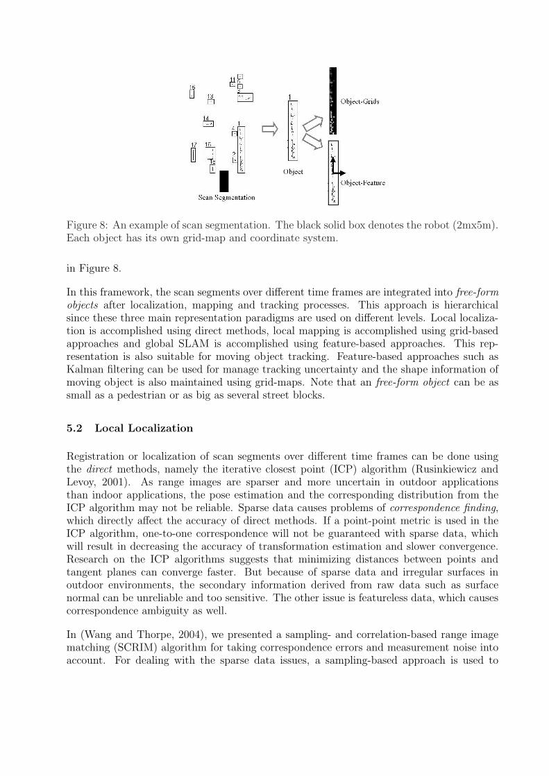
Figure 8: An example of scan segmentation. The black solid box denotes the robot (2mx5m).Each object has its own grid-map and coordinate system.

in Figure 8.

In this framework, the scan segments over different time frames are integrated into free-formobjects after localization, mapping and tracking processes. This approach is hierarchicalsince these three main representation paradigms are used on different levels. Local localiza-tion is accomplished using direct methods, local mapping is accomplished using grid-basedapproaches and global SLAM is accomplished using feature-based approaches. This rep-resentation is also suitable for moving object tracking. Feature-based approaches such asKalman filtering can be used for manage tracking uncertainty and the shape information ofmoving object is also maintained using grid-maps. Note that an free-form object can be assmall as a pedestrian or as big as several street blocks.

5.2 Local Localization

Registration or localization of scan segments over different time frames can be done usingthe direct methods, namely the iterative closest point (ICP) algorithm (Rusinkiewicz andLevoy, 2001). As range images are sparser and more uncertain in outdoor applicationsthan indoor applications, the pose estimation and the corresponding distribution from theICP algorithm may not be reliable. Sparse data causes problems of correspondence finding,which directly affect the accuracy of direct methods. If a point-point metric is used in theICP algorithm, one-to-one correspondence will not be guaranteed with sparse data, whichwill result in decreasing the accuracy of transformation estimation and slower convergence.Research on the ICP algorithms suggests that minimizing distances between points andtangent planes can converge faster. But because of sparse data and irregular surfaces inoutdoor environments, the secondary information derived from raw data such as surfacenormal can be unreliable and too sensitive. The other issue is featureless data, which causescorrespondence ambiguity as well.

In (Wang and Thorpe, 2004), we presented a sampling- and correlation-based range imagematching (SCRIM) algorithm for taking correspondence errors and measurement noise intoaccount. For dealing with the sparse data issues, a sampling-based approach is used to

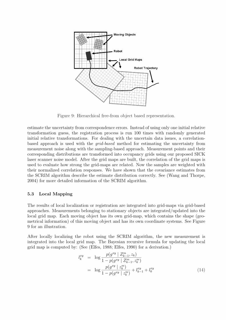
Figure 9: Hierarchical free-from object based representation.

estimate the uncertainty from correspondence errors. Instead of using only one initial relativetransformation guess, the registration process is run 100 times with randomly generatedinitial relative transformations. For dealing with the uncertain data issues, a correlation-based approach is used with the grid-based method for estimating the uncertainty frommeasurement noise along with the sampling-based approach. Measurement points and theircorresponding distributions are transformed into occupancy grids using our proposed SICKlaser scanner noise model. After the grid maps are built, the correlation of the grid maps isused to evaluate how strong the grid-maps are related. Now the samples are weighted withtheir normalized correlation responses. We have shown that the covariance estimates fromthe SCRIM algorithm describe the estimate distribution correctly. See (Wang and Thorpe,2004) for more detailed information of the SCRIM algorithm.

5.3 Local Mapping

The results of local localization or registration are integrated into grid-maps via grid-basedapproaches. Measurements belonging to stationary objects are integrated/updated into thelocal grid map. Each moving object has its own grid-map, which contains the shape (geo-metrical information) of this moving object and has its own coordinate systems. See Figure9 for an illustration.

After locally localizing the robot using the SCRIM algorithm, the new measurement isintegrated into the local grid map. The Bayesian recursive formula for updating the localgrid map is computed by: (See (Elfes, 1988; Elfes, 1990) for a derivation.)

lxyk = log

p(gxy | Zmk−1, zk)

1− p(gxy | Zmk−1, z

mk )

= logp(gxy | zm

k )

1− p(gxy | zmk )

+ lxyk−1 + lxy

0 (14)

−1200 −1000 −800 −600 −400−300

−200

−100

0

100

200

300

400

500

meter

met

er

1

2

3

4

5

6

7

8

9

10

1112

13

14

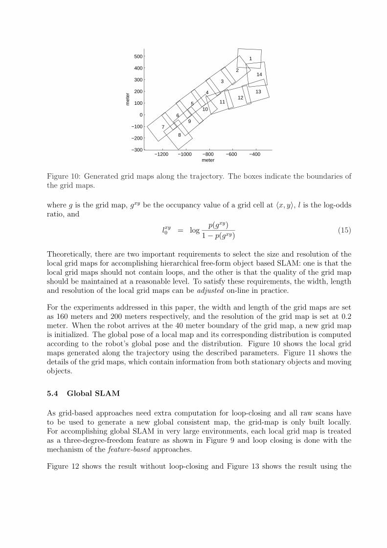
Figure 10: Generated grid maps along the trajectory. The boxes indicate the boundaries ofthe grid maps.

where g is the grid map, gxy be the occupancy value of a grid cell at 〈x, y〉, l is the log-oddsratio, and

lxy0 = log

p(gxy)

1− p(gxy)(15)

Theoretically, there are two important requirements to select the size and resolution of thelocal grid maps for accomplishing hierarchical free-form object based SLAM: one is that thelocal grid maps should not contain loops, and the other is that the quality of the grid mapshould be maintained at a reasonable level. To satisfy these requirements, the width, lengthand resolution of the local grid maps can be adjusted on-line in practice.

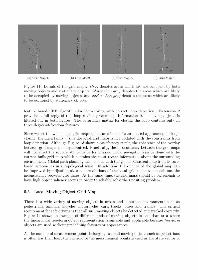
For the experiments addressed in this paper, the width and length of the grid maps are setas 160 meters and 200 meters respectively, and the resolution of the grid map is set at 0.2meter. When the robot arrives at the 40 meter boundary of the grid map, a new grid mapis initialized. The global pose of a local map and its corresponding distribution is computedaccording to the robot’s global pose and the distribution. Figure 10 shows the local gridmaps generated along the trajectory using the described parameters. Figure 11 shows thedetails of the grid maps, which contain information from both stationary objects and movingobjects.

5.4 Global SLAM

As grid-based approaches need extra computation for loop-closing and all raw scans haveto be used to generate a new global consistent map, the grid-map is only built locally.For accomplishing global SLAM in very large environments, each local grid map is treatedas a three-degree-freedom feature as shown in Figure 9 and loop closing is done with themechanism of the feature-based approaches.

Figure 12 shows the result without loop-closing and Figure 13 shows the result using the

(a) Grid Map 1. (b) Grid Map2. (c) Grid Map 3. (d) Grid Map 4.

Figure 11: Details of the grid maps. Gray denotes areas which are not occupied by bothmoving objects and stationary objects, whiter than gray denotes the areas which are likelyto be occupied by moving objects, and darker than gray denotes the areas which are likelyto be occupied by stationary objects.

feature based EKF algorithm for loop-closing with correct loop detection. Extension 2provides a full reply of this loop closing processing. Information from moving objects isfiltered out in both figures. The covariance matrix for closing this loop contains only 14three degree-of-freedom features.

Since we set the whole local grid maps as features in the feature-based approaches for loop-closing, the uncertainty inside the local grid maps is not updated with the constraints fromloop detection. Although Figure 13 shows a satisfactory result, the coherence of the overlaybetween grid maps is not guaranteed. Practically, the inconsistency between the grid-mapswill not effect the robot’s ability to perform tasks. Local navigation can be done with thecurrent built grid map which contains the most recent information about the surroundingenvironment. Global path planning can be done with the global consistent map from feature-based approaches in a topological sense. In addition, the quality of the global map canbe improved by adjusting sizes and resolutions of the local grid maps to smooth out theinconsistency between grid maps. At the same time, the grid-maps should be big enough tohave high object saliency scores in order to reliably solve the revisiting problem.

5.5 Local Moving Object Grid Map

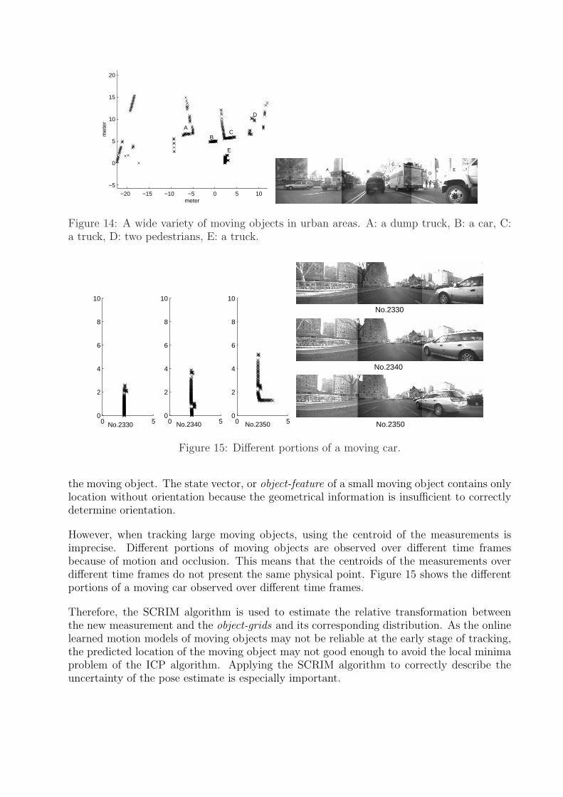
There is a wide variety of moving objects in urban and suburban environments such aspedestrians, animals, bicycles, motorcycles, cars, trucks, buses and trailers. The criticalrequirement for safe driving is that all such moving objects be detected and tracked correctly.Figure 14 shows an example of different kinds of moving objects in an urban area wherethe hierarchical free-form object representation is suitable and applicable because free-formobjects are used without predefining features or appearances.

As the number of measurement points belonging to small moving objects such as pedestriansis often less than four, the centroid of the measurement points is used as the state vector of

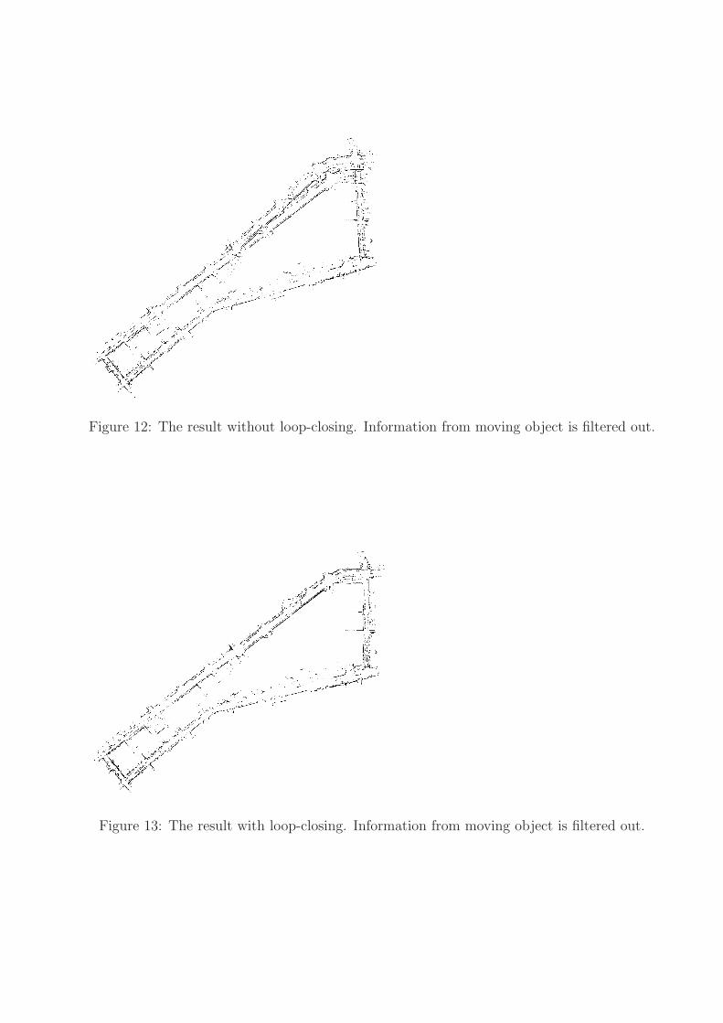
Figure 12: The result without loop-closing. Information from moving object is filtered out.

Figure 13: The result with loop-closing. Information from moving object is filtered out.

−20 −15 −10 −5 0 5 10

−5

0

5

10

15

20

meter

met

er A

B C

D

E

A B

C

D E

Figure 14: A wide variety of moving objects in urban areas. A: a dump truck, B: a car, C:a truck, D: two pedestrians, E: a truck.

0 50

2

4

6

8

10

0 50

2

4

6

8

10

0 50

2

4

6

8

10

No.2330 No.2340 No.2350

No.2330

No.2340

No.2350

Figure 15: Different portions of a moving car.

the moving object. The state vector, or object-feature of a small moving object contains onlylocation without orientation because the geometrical information is insufficient to correctlydetermine orientation.

However, when tracking large moving objects, using the centroid of the measurements isimprecise. Different portions of moving objects are observed over different time framesbecause of motion and occlusion. This means that the centroids of the measurements overdifferent time frames do not present the same physical point. Figure 15 shows the differentportions of a moving car observed over different time frames.

Therefore, the SCRIM algorithm is used to estimate the relative transformation betweenthe new measurement and the object-grids and its corresponding distribution. As the onlinelearned motion models of moving objects may not be reliable at the early stage of tracking,the predicted location of the moving object may not good enough to avoid the local minimaproblem of the ICP algorithm. Applying the SCRIM algorithm to correctly describe theuncertainty of the pose estimate is especially important.

−2 0 2 4 6

−2

−1

0

1

2

3

4

5

meterm

eter

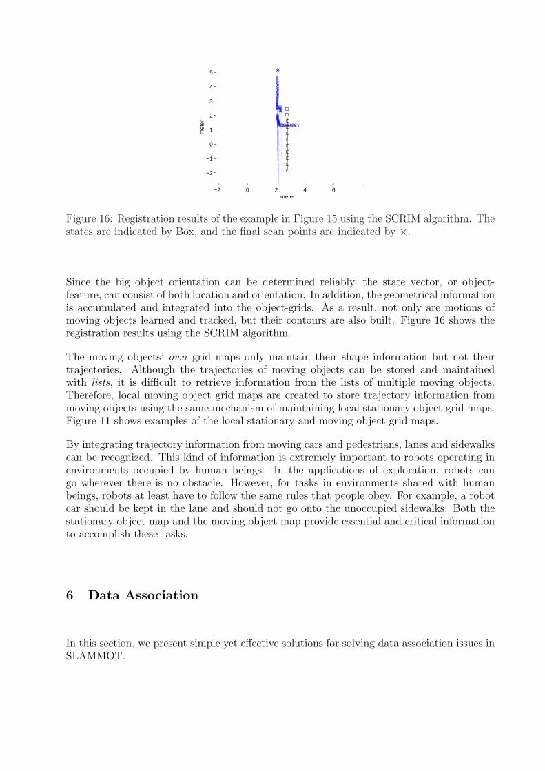
Figure 16: Registration results of the example in Figure 15 using the SCRIM algorithm. Thestates are indicated by Box, and the final scan points are indicated by ×.

Since the big object orientation can be determined reliably, the state vector, or object-feature, can consist of both location and orientation. In addition, the geometrical informationis accumulated and integrated into the object-grids. As a result, not only are motions ofmoving objects learned and tracked, but their contours are also built. Figure 16 shows theregistration results using the SCRIM algorithm.

The moving objects’ own grid maps only maintain their shape information but not theirtrajectories. Although the trajectories of moving objects can be stored and maintainedwith lists, it is difficult to retrieve information from the lists of multiple moving objects.Therefore, local moving object grid maps are created to store trajectory information frommoving objects using the same mechanism of maintaining local stationary object grid maps.Figure 11 shows examples of the local stationary and moving object grid maps.

By integrating trajectory information from moving cars and pedestrians, lanes and sidewalkscan be recognized. This kind of information is extremely important to robots operating inenvironments occupied by human beings. In the applications of exploration, robots cango wherever there is no obstacle. However, for tasks in environments shared with humanbeings, robots at least have to follow the same rules that people obey. For example, a robotcar should be kept in the lane and should not go onto the unoccupied sidewalks. Both thestationary object map and the moving object map provide essential and critical informationto accomplish these tasks.

6 Data Association

In this section, we present simple yet effective solutions for solving data association issues inSLAMMOT.

−1200 −1000 −800 −600 −400−300

−200

−100

0

100

200

300

400

500

600

meter

met

er

1516

17

18

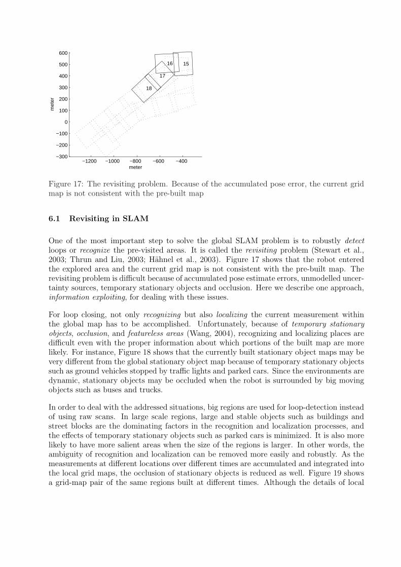
Figure 17: The revisiting problem. Because of the accumulated pose error, the current gridmap is not consistent with the pre-built map

6.1 Revisiting in SLAM

One of the most important step to solve the global SLAM problem is to robustly detectloops or recognize the pre-visited areas. It is called the revisiting problem (Stewart et al.,2003; Thrun and Liu, 2003; Hahnel et al., 2003). Figure 17 shows that the robot enteredthe explored area and the current grid map is not consistent with the pre-built map. Therevisiting problem is difficult because of accumulated pose estimate errors, unmodelled uncer-tainty sources, temporary stationary objects and occlusion. Here we describe one approach,information exploiting, for dealing with these issues.

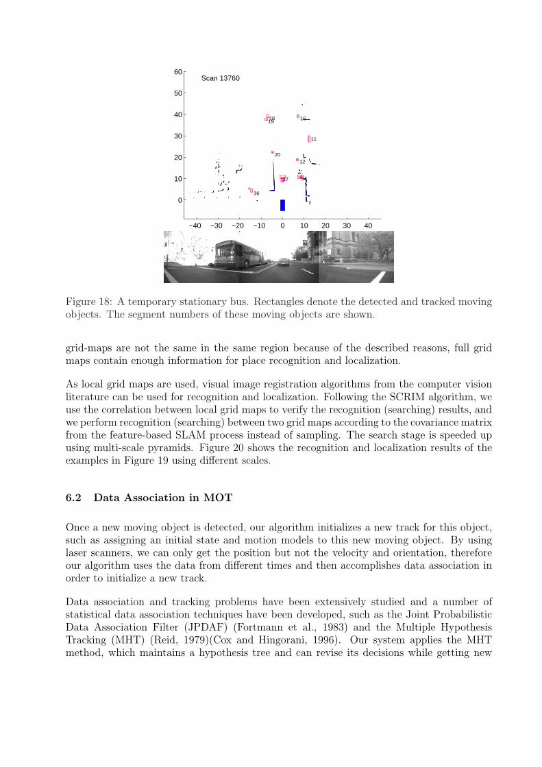
For loop closing, not only recognizing but also localizing the current measurement withinthe global map has to be accomplished. Unfortunately, because of temporary stationaryobjects, occlusion, and featureless areas (Wang, 2004), recognizing and localizing places aredifficult even with the proper information about which portions of the built map are morelikely. For instance, Figure 18 shows that the currently built stationary object maps may bevery different from the global stationary object map because of temporary stationary objectssuch as ground vehicles stopped by traffic lights and parked cars. Since the environments aredynamic, stationary objects may be occluded when the robot is surrounded by big movingobjects such as buses and trucks.

In order to deal with the addressed situations, big regions are used for loop-detection insteadof using raw scans. In large scale regions, large and stable objects such as buildings andstreet blocks are the dominating factors in the recognition and localization processes, andthe effects of temporary stationary objects such as parked cars is minimized. It is also morelikely to have more salient areas when the size of the regions is larger. In other words, theambiguity of recognition and localization can be removed more easily and robustly. As themeasurements at different locations over different times are accumulated and integrated intothe local grid maps, the occlusion of stationary objects is reduced as well. Figure 19 showsa grid-map pair of the same regions built at different times. Although the details of local

−40 −30 −20 −10 0 10 20 30 40

0

10

20

30

40

50

60

45

11

12

16

17

1819

20

36

Scan 13760

Figure 18: A temporary stationary bus. Rectangles denote the detected and tracked movingobjects. The segment numbers of these moving objects are shown.

grid-maps are not the same in the same region because of the described reasons, full gridmaps contain enough information for place recognition and localization.

As local grid maps are used, visual image registration algorithms from the computer visionliterature can be used for recognition and localization. Following the SCRIM algorithm, weuse the correlation between local grid maps to verify the recognition (searching) results, andwe perform recognition (searching) between two grid maps according to the covariance matrixfrom the feature-based SLAM process instead of sampling. The search stage is speeded upusing multi-scale pyramids. Figure 20 shows the recognition and localization results of theexamples in Figure 19 using different scales.

6.2 Data Association in MOT

Once a new moving object is detected, our algorithm initializes a new track for this object,such as assigning an initial state and motion models to this new moving object. By usinglaser scanners, we can only get the position but not the velocity and orientation, thereforeour algorithm uses the data from different times and then accomplishes data association inorder to initialize a new track.

Data association and tracking problems have been extensively studied and a number ofstatistical data association techniques have been developed, such as the Joint ProbabilisticData Association Filter (JPDAF) (Fortmann et al., 1983) and the Multiple HypothesisTracking (MHT) (Reid, 1979)(Cox and Hingorani, 1996). Our system applies the MHTmethod, which maintains a hypothesis tree and can revise its decisions while getting new

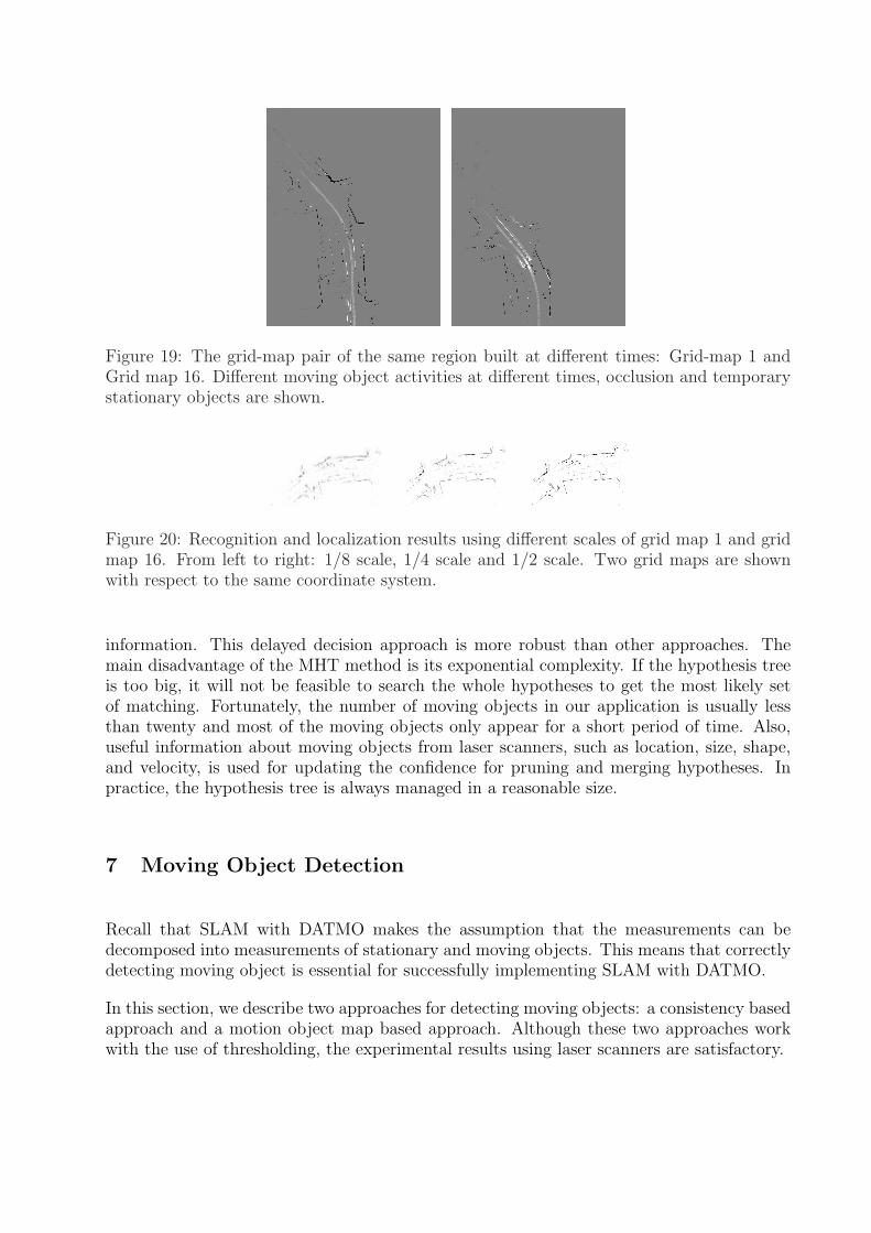
Figure 19: The grid-map pair of the same region built at different times: Grid-map 1 andGrid map 16. Different moving object activities at different times, occlusion and temporarystationary objects are shown.

Figure 20: Recognition and localization results using different scales of grid map 1 and gridmap 16. From left to right: 1/8 scale, 1/4 scale and 1/2 scale. Two grid maps are shownwith respect to the same coordinate system.

information. This delayed decision approach is more robust than other approaches. Themain disadvantage of the MHT method is its exponential complexity. If the hypothesis treeis too big, it will not be feasible to search the whole hypotheses to get the most likely setof matching. Fortunately, the number of moving objects in our application is usually lessthan twenty and most of the moving objects only appear for a short period of time. Also,useful information about moving objects from laser scanners, such as location, size, shape,and velocity, is used for updating the confidence for pruning and merging hypotheses. Inpractice, the hypothesis tree is always managed in a reasonable size.

7 Moving Object Detection

Recall that SLAM with DATMO makes the assumption that the measurements can bedecomposed into measurements of stationary and moving objects. This means that correctlydetecting moving object is essential for successfully implementing SLAM with DATMO.

In this section, we describe two approaches for detecting moving objects: a consistency basedapproach and a motion object map based approach. Although these two approaches workwith the use of thresholding, the experimental results using laser scanners are satisfactory.

−40 −30 −20 −10 0 10 20 30 40

0

10

20

30

40

50

60

meter

met

er

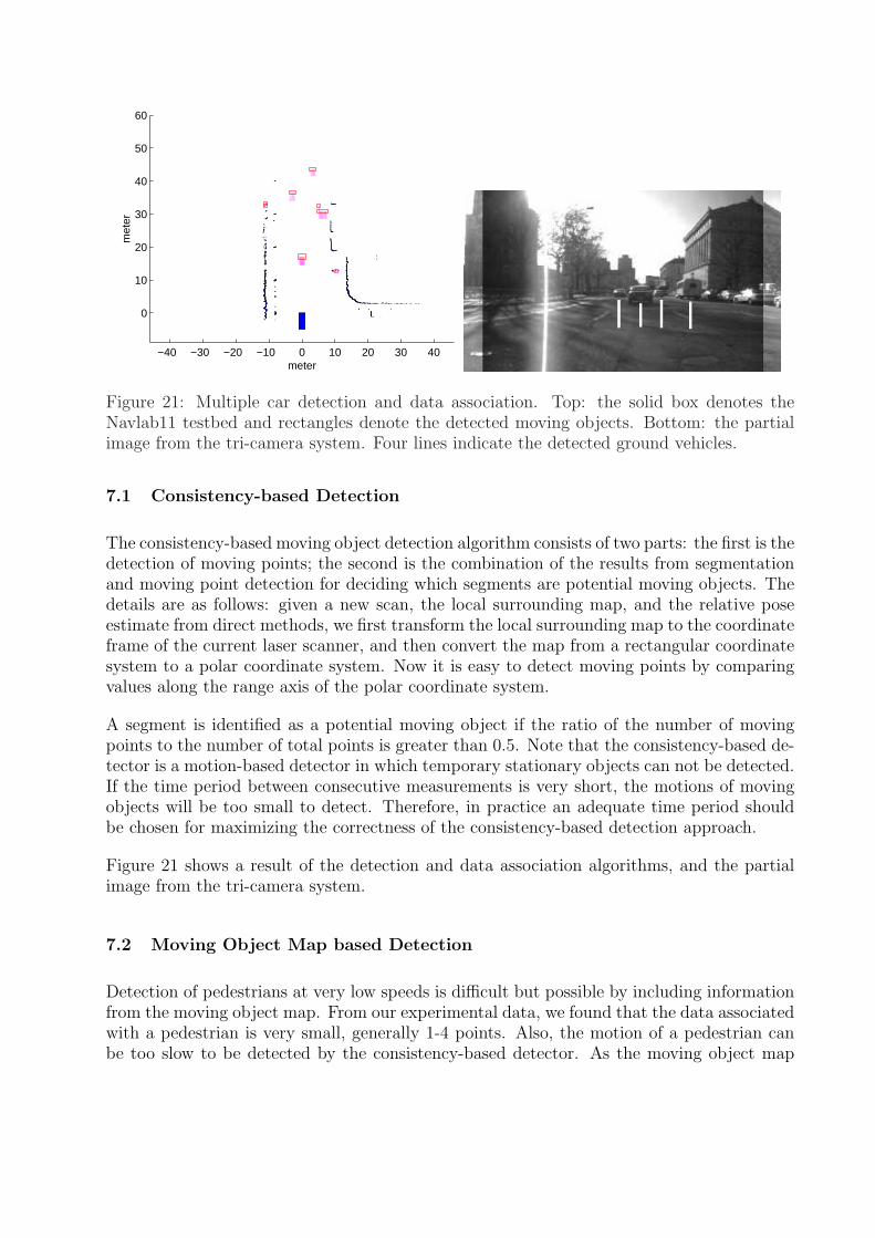
Figure 21: Multiple car detection and data association. Top: the solid box denotes theNavlab11 testbed and rectangles denote the detected moving objects. Bottom: the partialimage from the tri-camera system. Four lines indicate the detected ground vehicles.

7.1 Consistency-based Detection

The consistency-based moving object detection algorithm consists of two parts: the first is thedetection of moving points; the second is the combination of the results from segmentationand moving point detection for deciding which segments are potential moving objects. Thedetails are as follows: given a new scan, the local surrounding map, and the relative poseestimate from direct methods, we first transform the local surrounding map to the coordinateframe of the current laser scanner, and then convert the map from a rectangular coordinatesystem to a polar coordinate system. Now it is easy to detect moving points by comparingvalues along the range axis of the polar coordinate system.

A segment is identified as a potential moving object if the ratio of the number of movingpoints to the number of total points is greater than 0.5. Note that the consistency-based de-tector is a motion-based detector in which temporary stationary objects can not be detected.If the time period between consecutive measurements is very short, the motions of movingobjects will be too small to detect. Therefore, in practice an adequate time period shouldbe chosen for maximizing the correctness of the consistency-based detection approach.

Figure 21 shows a result of the detection and data association algorithms, and the partialimage from the tri-camera system.

7.2 Moving Object Map based Detection

Detection of pedestrians at very low speeds is difficult but possible by including informationfrom the moving object map. From our experimental data, we found that the data associatedwith a pedestrian is very small, generally 1-4 points. Also, the motion of a pedestrian canbe too slow to be detected by the consistency-based detector. As the moving object map

contains information from previous moving objects, we can say that if a blob is in an areathat was previously occupied by moving objects, this object can be recognized as a potentialmoving object.

8 Experimental results

So far we have shown the procedures in detail for accomplishing ladar-based SLAM withDATMO from a ground vehicle at high speeds in crowded urban areas. To summarize, Figure22 shows the flow diagram of SLAM with DATMO, and the steps are briefly described below:

8.0.1 Data collecting and preprocessing

Measurements from motion sensors such as odometry and measurements from perceptionsensors such as laser scanners are collected. In our applications, laser scans are segmented.The robot pose is predicted using the motion measurement and the robot motion model.

8.0.2 Tracked moving object association

The scan segments are associated with the tracked moving objects with the MHT algorithm.In this stage, the predicted robot pose estimate is used.

8.0.3 Moving object detection and robot pose estimation

Only scan segments not associated with the tracked moving objects are used in this stage.Two algorithms, the consistency-based and the moving object map-based detectors, are usedto detect moving objects. At the same time, the robot pose estimate is improved with theuse of the SCRIM algorithm.

8.0.4 Update of stationary and moving objects

With the updated robot pose estimate, the tracked moving objects are updated and the newmoving objects are initialized via the IMM algorithm. If the robot arrives the boundaryof the local grid map, a new stationary object grid map and a new moving object gridmap are initialized and the global SLAM using feature-based approaches stages is activated.Otherwise, the stationary object grid map and the moving object grid map are updated withthe new stationary scan segments and the new moving scan segments, respectively. Now wecomplete one cycle of local localization, mapping and moving object tracking.

8.0.5 Global SLAM

The revisiting problem is solved. The local grid maps are treated as three degree-of-freedomfeatures and the global SLAM problem is solved via extended Kalman filtering.

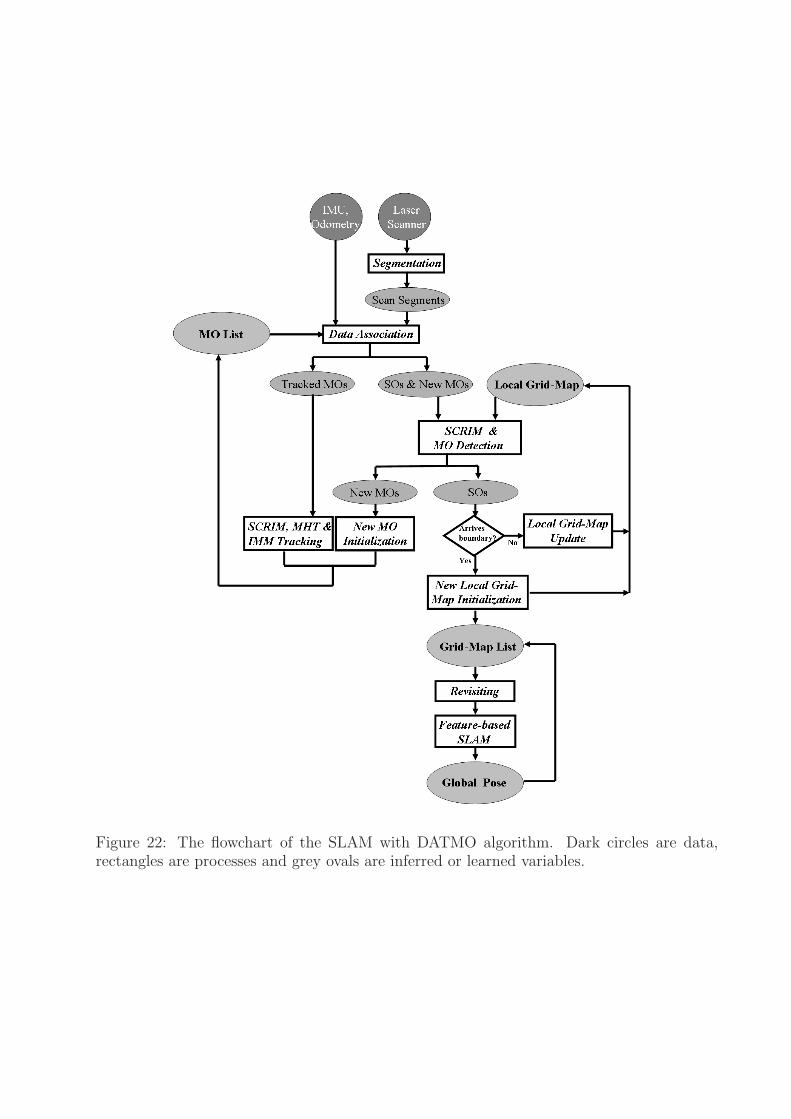
Figure 22: The flowchart of the SLAM with DATMO algorithm. Dark circles are data,rectangles are processes and grey ovals are inferred or learned variables.

0 10 20 30 40 50 60 70 80 90−15

−10

−5

0

5

10

15

X (meter)

−Y

(m

eter

)

Object A

Object B

Object C

Object D

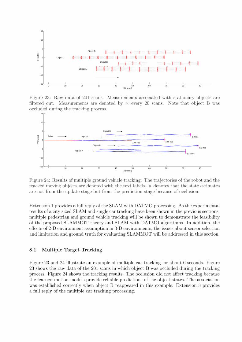
Figure 23: Raw data of 201 scans. Measurements associated with stationary objects arefiltered out. Measurements are denoted by × every 20 scans. Note that object B wasoccluded during the tracking process.

0 10 20 30 40 50 60 70 80 90−15

−10

−5

0

5

10

15

X (meter)

−Y

(m

eter

)

10.6 m/s

10.5 m/s

9.8 m/s

10.6 m/s

9.2 m/sRobot

Object A

Object B

Object C

Object D

Figure 24: Results of multiple ground vehicle tracking. The trajectories of the robot and thetracked moving objects are denoted with the text labels. × denotes that the state estimatesare not from the update stage but from the prediction stage because of occlusion.

Extension 1 provides a full reply of the SLAM with DATMO processing. As the experimentalresults of a city sized SLAM and single car tracking have been shown in the previous sections,multiple pedestrian and ground vehicle tracking will be shown to demonstrate the feasibilityof the proposed SLAMMOT theory and SLAM with DATMO algorithms. In addition, theeffects of 2-D environment assumption in 3-D environments, the issues about sensor selectionand limitation and ground truth for evaluating SLAMMOT will be addressed in this section.

8.1 Multiple Target Tracking

Figure 23 and 24 illustrate an example of multiple car tracking for about 6 seconds. Figure23 shows the raw data of the 201 scans in which object B was occluded during the trackingprocess. Figure 24 shows the tracking results. The occlusion did not affect tracking becausethe learned motion models provide reliable predictions of the object states. The associationwas established correctly when object B reappeared in this example. Extension 3 providesa full reply of the multiple car tracking processing.

−40 −30 −20 −10 0 10 20 30 40

0

10

20

30

40

50

60

meter

met

er

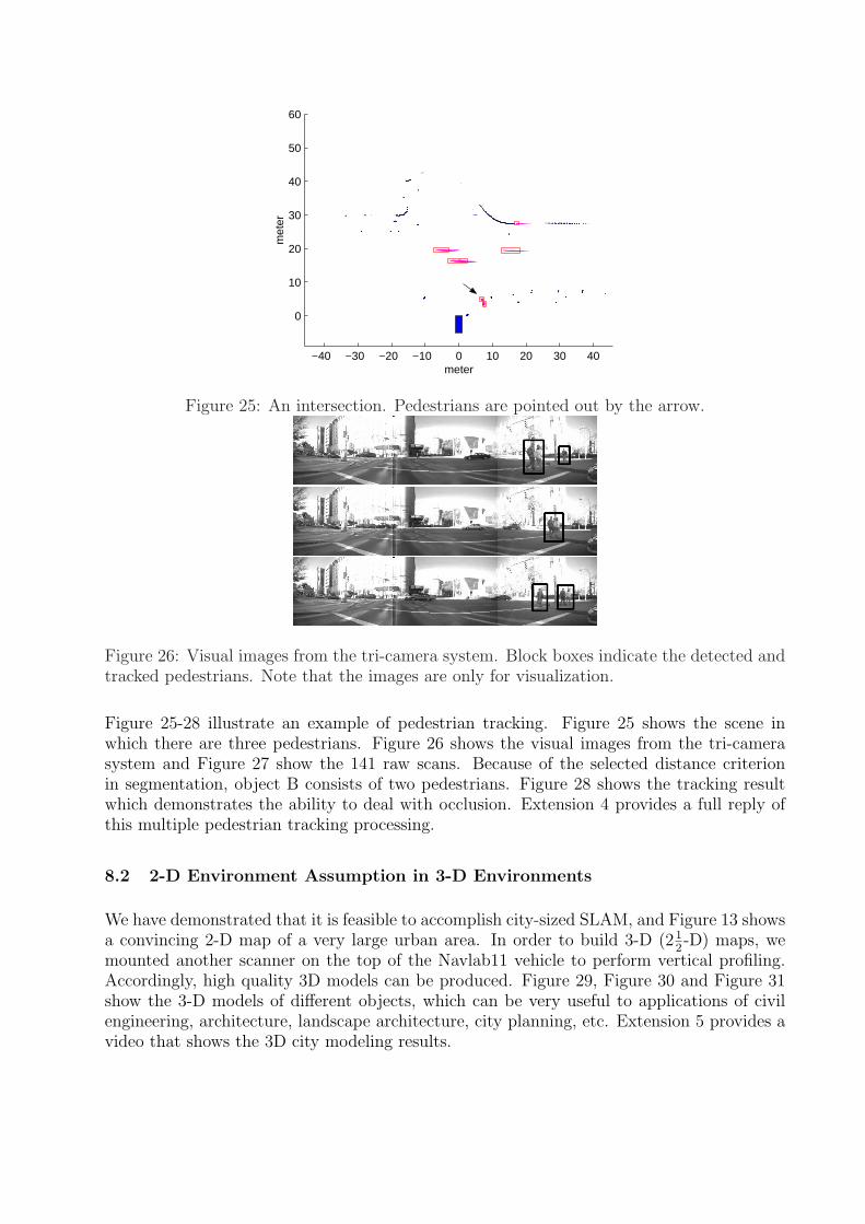
Figure 25: An intersection. Pedestrians are pointed out by the arrow.

Figure 26: Visual images from the tri-camera system. Block boxes indicate the detected andtracked pedestrians. Note that the images are only for visualization.

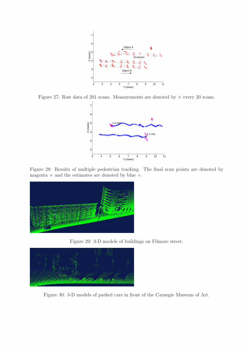
Figure 25-28 illustrate an example of pedestrian tracking. Figure 25 shows the scene inwhich there are three pedestrians. Figure 26 shows the visual images from the tri-camerasystem and Figure 27 show the 141 raw scans. Because of the selected distance criterionin segmentation, object B consists of two pedestrians. Figure 28 shows the tracking resultwhich demonstrates the ability to deal with occlusion. Extension 4 provides a full reply ofthis multiple pedestrian tracking processing.

8.2 2-D Environment Assumption in 3-D Environments

We have demonstrated that it is feasible to accomplish city-sized SLAM, and Figure 13 showsa convincing 2-D map of a very large urban area. In order to build 3-D (21

2-D) maps, we

mounted another scanner on the top of the Navlab11 vehicle to perform vertical profiling.Accordingly, high quality 3D models can be produced. Figure 29, Figure 30 and Figure 31show the 3-D models of different objects, which can be very useful to applications of civilengineering, architecture, landscape architecture, city planning, etc. Extension 5 provides avideo that shows the 3D city modeling results.

3 4 5 6 7 8 9 10 11

2

3

4

5

6

7

Y (meter)X

(m

eter

)

Object A

Object B

Occlusion

Figure 27: Raw data of 201 scans. Measurements are denoted by × every 20 scans.

3 4 5 6 7 8 9 10 11

2

3

4

5

6

7

Y (meter)

X (

met

er) 1.4 m/s

2.1 m/s

Figure 28: Results of multiple pedestrian tracking. The final scan points are denoted bymagenta × and the estimates are denoted by blue +.

Figure 29: 3-D models of buildings on Filmore street.

Figure 30: 3-D models of parked cars in front of the Carnegie Museum of Art.

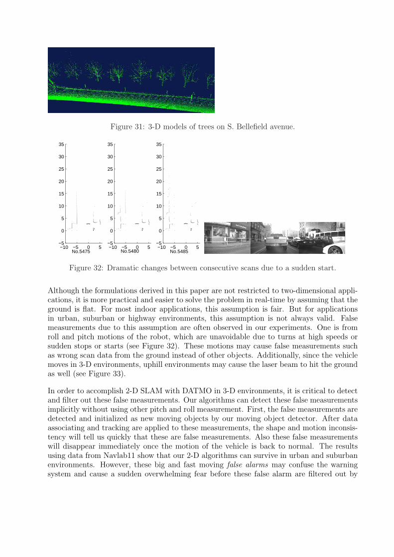
Figure 31: 3-D models of trees on S. Bellefield avenue.

−10 −5 0 5−5

0

5

10

15

20

25

30

35

−10 −5 0 5−5

0

5

10

15

20

25

30

35

−10 −5 0 5−5

0

5

10

15

20

25

30

35

No.5475 No.5480 No.5485

Figure 32: Dramatic changes between consecutive scans due to a sudden start.

Although the formulations derived in this paper are not restricted to two-dimensional appli-cations, it is more practical and easier to solve the problem in real-time by assuming that theground is flat. For most indoor applications, this assumption is fair. But for applicationsin urban, suburban or highway environments, this assumption is not always valid. Falsemeasurements due to this assumption are often observed in our experiments. One is fromroll and pitch motions of the robot, which are unavoidable due to turns at high speeds orsudden stops or starts (see Figure 32). These motions may cause false measurements suchas wrong scan data from the ground instead of other objects. Additionally, since the vehiclemoves in 3-D environments, uphill environments may cause the laser beam to hit the groundas well (see Figure 33).

In order to accomplish 2-D SLAM with DATMO in 3-D environments, it is critical to detectand filter out these false measurements. Our algorithms can detect these false measurementsimplicitly without using other pitch and roll measurement. First, the false measurements aredetected and initialized as new moving objects by our moving object detector. After dataassociating and tracking are applied to these measurements, the shape and motion inconsis-tency will tell us quickly that these are false measurements. Also these false measurementswill disappear immediately once the motion of the vehicle is back to normal. The resultsusing data from Navlab11 show that our 2-D algorithms can survive in urban and suburbanenvironments. However, these big and fast moving false alarms may confuse the warningsystem and cause a sudden overwhelming fear before these false alarm are filtered out by

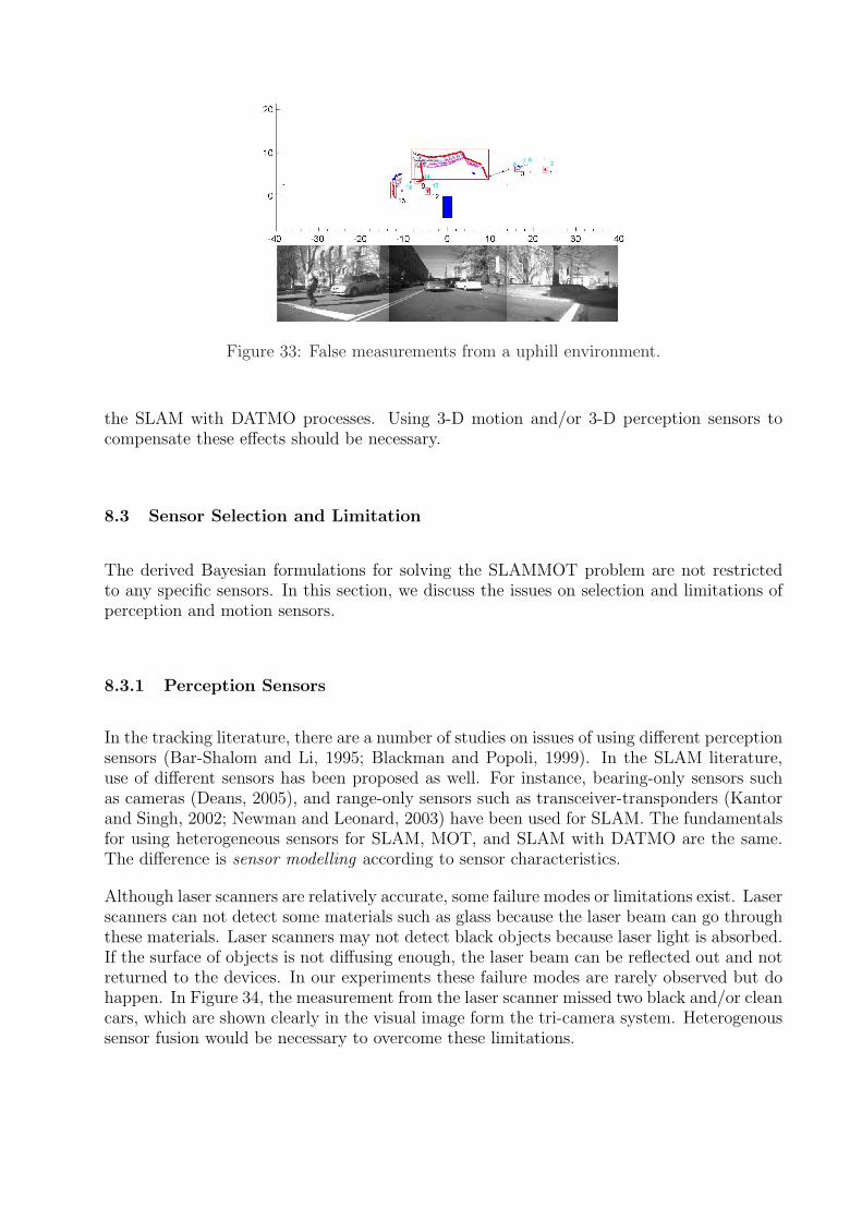
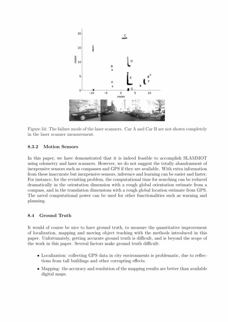
Figure 33: False measurements from a uphill environment.

the SLAM with DATMO processes. Using 3-D motion and/or 3-D perception sensors tocompensate these effects should be necessary.

8.3 Sensor Selection and Limitation

The derived Bayesian formulations for solving the SLAMMOT problem are not restrictedto any specific sensors. In this section, we discuss the issues on selection and limitations ofperception and motion sensors.

8.3.1 Perception Sensors

In the tracking literature, there are a number of studies on issues of using different perceptionsensors (Bar-Shalom and Li, 1995; Blackman and Popoli, 1999). In the SLAM literature,use of different sensors has been proposed as well. For instance, bearing-only sensors suchas cameras (Deans, 2005), and range-only sensors such as transceiver-transponders (Kantorand Singh, 2002; Newman and Leonard, 2003) have been used for SLAM. The fundamentalsfor using heterogeneous sensors for SLAM, MOT, and SLAM with DATMO are the same.The difference is sensor modelling according to sensor characteristics.

Although laser scanners are relatively accurate, some failure modes or limitations exist. Laserscanners can not detect some materials such as glass because the laser beam can go throughthese materials. Laser scanners may not detect black objects because laser light is absorbed.If the surface of objects is not diffusing enough, the laser beam can be reflected out and notreturned to the devices. In our experiments these failure modes are rarely observed but dohappen. In Figure 34, the measurement from the laser scanner missed two black and/or cleancars, which are shown clearly in the visual image form the tri-camera system. Heterogenoussensor fusion would be necessary to overcome these limitations.

−10 −5 0 5 100

5

10

15

20

meter

met

er

A

B

C

D

E F

G

A B C D

E F

G

Figure 34: The failure mode of the laser scanners. Car A and Car B are not shown completelyin the laser scanner measurement.

8.3.2 Motion Sensors

In this paper, we have demonstrated that it is indeed feasible to accomplish SLAMMOTusing odometry and laser scanners. However, we do not suggest the totally abandonment ofinexpensive sensors such as compasses and GPS if they are available. With extra informationfrom these inaccurate but inexpensive sensors, inference and learning can be easier and faster.For instance, for the revisiting problem, the computational time for searching can be reduceddramatically in the orientation dimension with a rough global orientation estimate from acompass, and in the translation dimensions with a rough global location estimate from GPS.The saved computational power can be used for other functionalities such as warning andplanning.

8.4 Ground Truth

It would of course be nice to have ground truth, to measure the quantitative improvementof localization, mapping and moving object tracking with the methods introduced in thispaper. Unfortunately, getting accurate ground truth is difficult, and is beyond the scope ofthe work in this paper. Several factors make ground truth difficult:

• Localization: collecting GPS data in city environments is problematic, due to reflec-tions from tall buildings and other corrupting effects.

• Mapping: the accuracy and resolution of the mapping results are better than availabledigital maps.

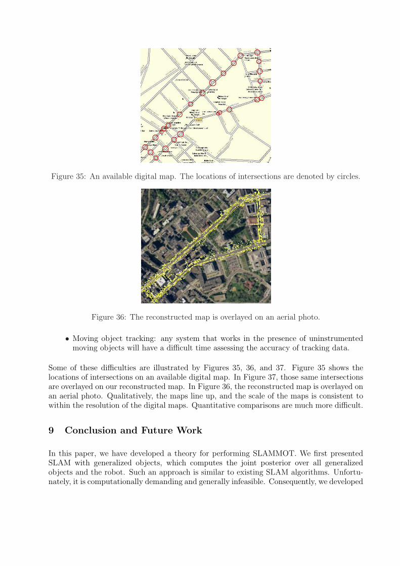
Figure 35: An available digital map. The locations of intersections are denoted by circles.

Figure 36: The reconstructed map is overlayed on an aerial photo.

• Moving object tracking: any system that works in the presence of uninstrumentedmoving objects will have a difficult time assessing the accuracy of tracking data.

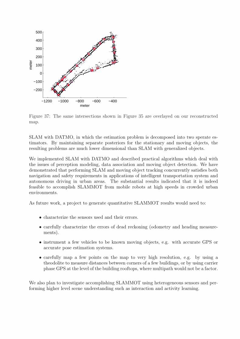
Some of these difficulties are illustrated by Figures 35, 36, and 37. Figure 35 shows thelocations of intersections on an available digital map. In Figure 37, those same intersectionsare overlayed on our reconstructed map. In Figure 36, the reconstructed map is overlayed onan aerial photo. Qualitatively, the maps line up, and the scale of the maps is consistent towithin the resolution of the digital maps. Quantitative comparisons are much more difficult.

9 Conclusion and Future Work

In this paper, we have developed a theory for performing SLAMMOT. We first presentedSLAM with generalized objects, which computes the joint posterior over all generalizedobjects and the robot. Such an approach is similar to existing SLAM algorithms. Unfortu-nately, it is computationally demanding and generally infeasible. Consequently, we developed

−1200 −1000 −800 −600 −400

−200

−100

0

100

200

300

400

500

meter

met

er

Figure 37: The same intersections shown in Figure 35 are overlayed on our reconstructedmap.

SLAM with DATMO, in which the estimation problem is decomposed into two sperate es-timators. By maintaining separate posteriors for the stationary and moving objects, theresulting problems are much lower dimensional than SLAM with generalized objects.

We implemented SLAM with DATMO and described practical algorithms which deal withthe issues of perception modeling, data association and moving object detection. We havedemonstrated that performing SLAM and moving object tracking concurrently satisfies bothnavigation and safety requirements in applications of intelligent transportation system andautonomous driving in urban areas. The substantial results indicated that it is indeedfeasible to accomplish SLAMMOT from mobile robots at high speeds in crowded urbanenvironments.

As future work, a project to generate quantitative SLAMMOT results would need to:

• characterize the sensors used and their errors.

• carefully characterize the errors of dead reckoning (odometry and heading measure-ments).

• instrument a few vehicles to be known moving objects, e.g. with accurate GPS oraccurate pose estimation systems.

• carefully map a few points on the map to very high resolution, e.g. by using atheodolite to measure distances between corners of a few buildings, or by using carrierphase GPS at the level of the building rooftops, where multipath would not be a factor.

We also plan to investigate accomplishing SLAMMOT using heterogeneous sensors and per-forming higher level scene understanding such as interaction and activity learning.

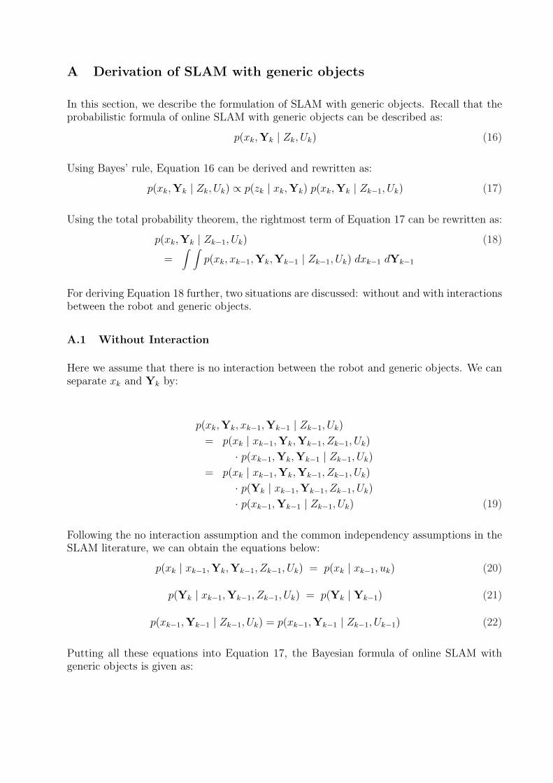
A Derivation of SLAM with generic objects

In this section, we describe the formulation of SLAM with generic objects. Recall that theprobabilistic formula of online SLAM with generic objects can be described as:

p(xk,Yk | Zk, Uk) (16)

Using Bayes’ rule, Equation 16 can be derived and rewritten as:

p(xk,Yk | Zk, Uk) ∝ p(zk | xk,Yk) p(xk,Yk | Zk−1, Uk) (17)

Using the total probability theorem, the rightmost term of Equation 17 can be rewritten as:

p(xk,Yk | Zk−1, Uk) (18)

=∫ ∫

p(xk, xk−1,Yk,Yk−1 | Zk−1, Uk) dxk−1 dYk−1

For deriving Equation 18 further, two situations are discussed: without and with interactionsbetween the robot and generic objects.

A.1 Without Interaction

Here we assume that there is no interaction between the robot and generic objects. We canseparate xk and Yk by:

p(xk,Yk, xk−1,Yk−1 | Zk−1, Uk)

= p(xk | xk−1,Yk,Yk−1, Zk−1, Uk)

· p(xk−1,Yk,Yk−1 | Zk−1, Uk)

= p(xk | xk−1,Yk,Yk−1, Zk−1, Uk)

· p(Yk | xk−1,Yk−1, Zk−1, Uk)

· p(xk−1,Yk−1 | Zk−1, Uk) (19)

Following the no interaction assumption and the common independency assumptions in theSLAM literature, we can obtain the equations below:

p(xk | xk−1,Yk,Yk−1, Zk−1, Uk) = p(xk | xk−1, uk) (20)

p(Yk | xk−1,Yk−1, Zk−1, Uk) = p(Yk | Yk−1) (21)

p(xk−1,Yk−1 | Zk−1, Uk) = p(xk−1,Yk−1 | Zk−1, Uk−1) (22)

Putting all these equations into Equation 17, the Bayesian formula of online SLAM withgeneric objects is given as:

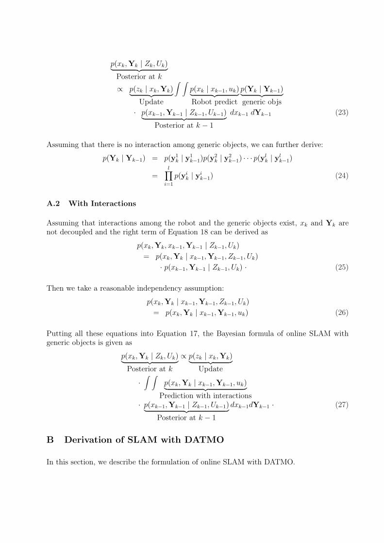
p(xk,Yk | Zk, Uk)︸︷︷︸Posterior at k


∫ ∫p(xk | xk−1, uk)︸︷︷︸Robot predict

p(Yk | Yk−1)︸︷︷︸generic objs


dxk−1 dYk−1 (23)

Assuming that there is no interaction among generic objects, we can further derive:

p(Yk | Yk−1) = p(y1k | y1

k−1)p(y2k | y2

k−1) · · · p(ylk | yl

k−1)

=l∏

i=1

p(yik | yi

k−1) (24)

A.2 With Interactions

Assuming that interactions among the robot and the generic objects exist, xk and Yk arenot decoupled and the right term of Equation 18 can be derived as

p(xk,Yk, xk−1,Yk−1 | Zk−1, Uk)

= p(xk,Yk | xk−1,Yk−1, Zk−1, Uk)

· p(xk−1,Yk−1 | Zk−1, Uk) · (25)

Then we take a reasonable independency assumption:

p(xk,Yk | xk−1,Yk−1, Zk−1, Uk)

= p(xk,Yk | xk−1,Yk−1, uk) (26)

Putting all these equations into Equation 17, the Bayesian formula of online SLAM withgeneric objects is given as

p(xk,Yk | Zk, Uk)︸︷︷︸Posterior at k


·∫ ∫

p(xk,Yk | xk−1,Yk−1, uk)︸︷︷︸Prediction with interactions


dxk−1dYk−1 · (27)

B Derivation of SLAM with DATMO

In this section, we describe the formulation of online SLAM with DATMO.

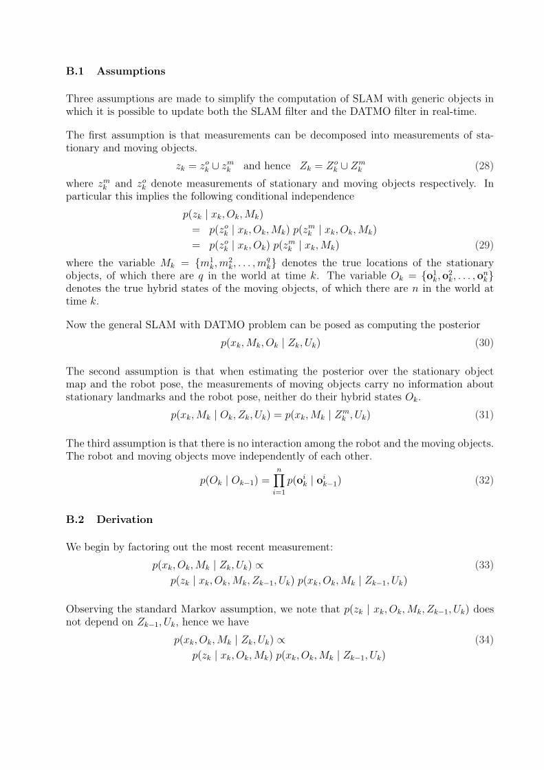
B.1 Assumptions

Three assumptions are made to simplify the computation of SLAM with generic objects inwhich it is possible to update both the SLAM filter and the DATMO filter in real-time.

The first assumption is that measurements can be decomposed into measurements of sta-tionary and moving objects.

zk = zok ∪ zm

k and hence Zk = Zok ∪ Zm

k (28)

where zmk and zo

k denote measurements of stationary and moving objects respectively. Inparticular this implies the following conditional independence

p(zk | xk, Ok,Mk)

= p(zok | xk, Ok, Mk) p(zm

k | xk, Ok,Mk)

= p(zok | xk, Ok) p(zm

k | xk,Mk) (29)

where the variable Mk = {m1k,m

2k, . . . , m

qk} denotes the true locations of the stationary

objects, of which there are q in the world at time k. The variable Ok = {o1k,o

2k, . . . ,o

nk}

denotes the true hybrid states of the moving objects, of which there are n in the world attime k.

Now the general SLAM with DATMO problem can be posed as computing the posterior

p(xk,Mk, Ok | Zk, Uk) (30)

The second assumption is that when estimating the posterior over the stationary objectmap and the robot pose, the measurements of moving objects carry no information aboutstationary landmarks and the robot pose, neither do their hybrid states Ok.

p(xk,Mk | Ok, Zk, Uk) = p(xk,Mk | Zmk , Uk) (31)

The third assumption is that there is no interaction among the robot and the moving objects.The robot and moving objects move independently of each other.

p(Ok | Ok−1) =n∏

i=1

p(oik | oi

k−1) (32)

B.2 Derivation

We begin by factoring out the most recent measurement:

p(xk, Ok,Mk | Zk, Uk) ∝ (33)

p(zk | xk, Ok,Mk, Zk−1, Uk) p(xk, Ok,Mk | Zk−1, Uk)

Observing the standard Markov assumption, we note that p(zk | xk, Ok, Mk, Zk−1, Uk) doesnot depend on Zk−1, Uk, hence we have

p(xk, Ok,Mk | Zk, Uk) ∝ (34)

p(zk | xk, Ok,Mk) p(xk, Ok,Mk | Zk−1, Uk)

·∫

p(Ok | Ok−1) p(Ok−1 | Zok−1, Uk−1) dOk−1

︸︷︷︸DATMO Prediction

· p(zmk | Mk, xk)︸︷︷︸

SLAM Update

·∫

p(xk | uk, xk−1) p(xk−1, Mk−1 | Zmk−1, Uk−1) dxk−1

︸︷︷︸SLAM Prediction

From Equation 40, input to this SLAM with DATMO filter are two separate posteriors, oneof the conventional SLAM form and a separate one for DATMO. How to recover those SLAMand DATMO posteriors at time k is simple.

For the SLAM part, we get

p(xk,Mk | Zmk , Uk) (41)

=∫

p(Ok,Mk, xk | Zk, Uk) dOk

∝ p(zmk | Mk, xk) ·∫p(xk | uk, xk−1) p(xk−1, Mk−1 | Zm

k−1, Uk−1) dxk−1

For the DATMO part , we get

p(Ok | Zk, Uk) (42)

=∫ ∫

p(Ok, Mk, xk | Zk, Uk)dMkdxk

∝∫

(p(zok | Ok, xk)

∫p(Ok | Ok−1)

p(Ok−1 | Zok−1, Uk−1)dOk−1)p(xk | Zm

k , Uk)dxk

where the posterior over the pose p(xk | Zmk , Uk) is simply the marginal of the joint calculated

in Equation 41:

p(xk | Zmk , Uk) =

∫p(xk,Mk | Zm

k , Uk)dMk (43)

C Index to Multimedia Extensions

The multimedia extensions to this article are at: http://www.ijrr.org. Extension 1 is a videothat illustrates the processing of the SLAM with DATMO approach (Figure 22). Extension2 is a video that shows the processing of loop closing (Figure 13). Extension 3 and 4 arethe videos illustrate the processing of multiple vehicle tracking (Figure 24) and multiplepedestrian tracking (Figure 28), respectively. Extension 5 is a video shows the 3D citymodeling results (Figure 29, Figure 30 and Figure 31).

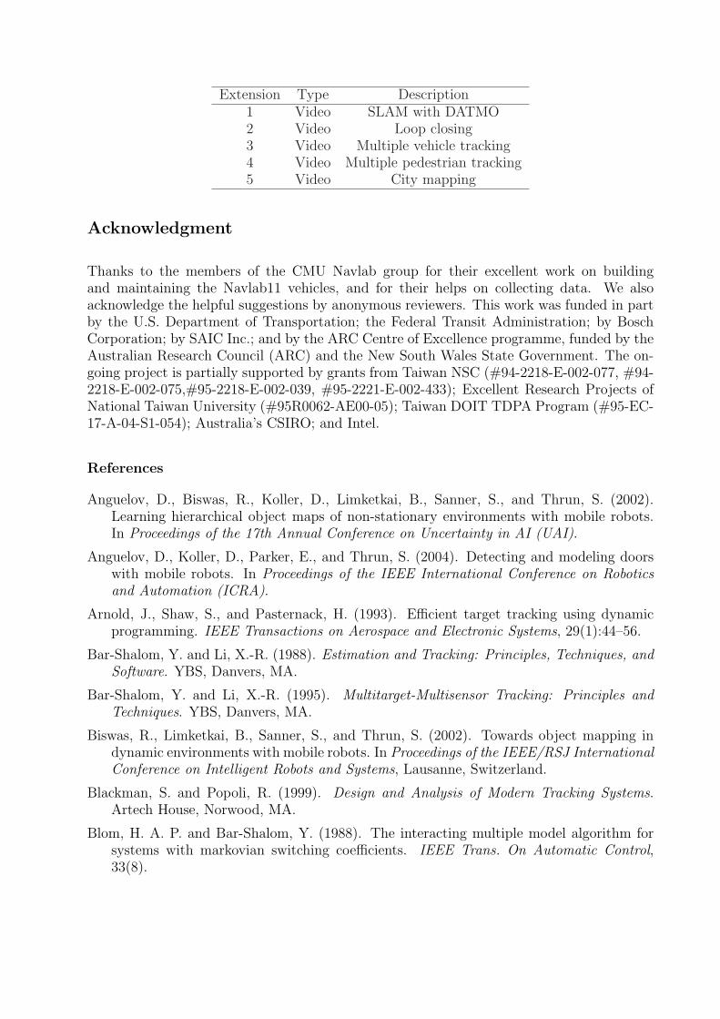
Extension Type Description1 Video SLAM with DATMO2 Video Loop closing3 Video Multiple vehicle tracking4 Video Multiple pedestrian tracking5 Video City mapping

Acknowledgment

Thanks to the members of the CMU Navlab group for their excellent work on buildingand maintaining the Navlab11 vehicles, and for their helps on collecting data. We alsoacknowledge the helpful suggestions by anonymous reviewers. This work was funded in partby the U.S. Department of Transportation; the Federal Transit Administration; by BoschCorporation; by SAIC Inc.; and by the ARC Centre of Excellence programme, funded by theAustralian Research Council (ARC) and the New South Wales State Government. The on-going project is partially supported by grants from Taiwan NSC (#94-2218-E-002-077, #94-2218-E-002-075,#95-2218-E-002-039, #95-2221-E-002-433); Excellent Research Projects ofNational Taiwan University (#95R0062-AE00-05); Taiwan DOIT TDPA Program (#95-EC-17-A-04-S1-054); Australia’s CSIRO; and Intel.

References

Anguelov, D., Biswas, R., Koller, D., Limketkai, B., Sanner, S., and Thrun, S. (2002).Learning hierarchical object maps of non-stationary environments with mobile robots.In Proceedings of the 17th Annual Conference on Uncertainty in AI (UAI).

Anguelov, D., Koller, D., Parker, E., and Thrun, S. (2004). Detecting and modeling doorswith mobile robots. In Proceedings of the IEEE International Conference on Roboticsand Automation (ICRA).

Arnold, J., Shaw, S., and Pasternack, H. (1993). Efficient target tracking using dynamicprogramming. IEEE Transactions on Aerospace and Electronic Systems, 29(1):44–56.

Bar-Shalom, Y. and Li, X.-R. (1988). Estimation and Tracking: Principles, Techniques, andSoftware. YBS, Danvers, MA.

Bar-Shalom, Y. and Li, X.-R. (1995). Multitarget-Multisensor Tracking: Principles andTechniques. YBS, Danvers, MA.

Biswas, R., Limketkai, B., Sanner, S., and Thrun, S. (2002). Towards object mapping indynamic environments with mobile robots. In Proceedings of the IEEE/RSJ InternationalConference on Intelligent Robots and Systems, Lausanne, Switzerland.

Blackman, S. and Popoli, R. (1999). Design and Analysis of Modern Tracking Systems.Artech House, Norwood, MA.

Blom, H. A. P. and Bar-Shalom, Y. (1988). The interacting multiple model algorithm forsystems with markovian switching coefficients. IEEE Trans. On Automatic Control,33(8).

Bosse, M., Newman, P., Leonard, J., Soika, M., Feiten, W., and Teller, S. (2003). An atlasframework for scalavle mapping. In Proceedings of the IEEE International Conferenceon Robotics and Automation (ICRA), Taipei, Taiwan.

Brand, M. (2001). Morphable 3d models from video. In Proceedings of the IEEE Conferenceon Computer Vision and Pattern Recognition.

Bregler, C., Hertzmann, A., and Biermann, H. (2000). Recovering non-rigid 3d shape fromimage streams. In Proceedings of the IEEE Conference on Computer Vision and PatternRecognition.

Choset, H. and Nagatani, K. (2001). Topological simultaneous localization and mapping(slam): Toward exact localization without explicit localization. IEEE Transactions onRobotics and Automation, 17(2):125–136.

Christensen, H. I., editor (2002). Lecture Notes: SLAM Summer School 2002.

Coraluppi, S. and Carthel, C. (2001). Multiple-hypothesis IMM (MH-IMM) filter for movingand stationary targets. In Proceedings of the International Conference on InformationFusion, pages TuB1–18–23, Montreal, QC, Canada.

Coraluppi, S., Luettgen, M., and Carthel, C. (2000). A hybrid-state estimation algorithmfor multi-sensor target tracking. In Proceedings of the International Conference on In-formation Fusion, pages TuB1–18–23, Paris, France.

Cox, I. J. and Hingorani, S. L. (1996). An efficient implemenation of Reid’s multiple hy-pothesis tracking algorithm and its evaluation for the purpose of visual tracking. IEEETrans. on Pattern Analysis and Machine intelligence, 18(2).

Deans, M. C. (2005). Bearings-Only Localization and Mapping. PhD thesis, The RoboticsInstitute, Carnegie Mellon University, Pittsburgh, PA.

Dellaert, F., Burgard, W., Fox, D., and Thrun, S. (1999). Using the condensation algorithmfor robust, vision-based mobile robot localization. IEEE Computer Society Conferenceon Computer Vision and Pattern Recognition ( CVPR’99 ).

Demirdjian, D. and Horaud, R. (2000). Motion-egomotion discrimination and motion seg-mentation from image-pair streams. Computer Vision and Image Understanding, pages53–68.

Durrant-Whyte, H., Majumder, S., Thrun, S., de Battista, M., and Scheding, S. (2003).A bayesian algorithm for simultaneous localization and map building. In The tenthInternational Symposium on Robotics Research, volume 6, pages 44–66.

Elfes, A. (1988). Occupancy Grids as a Spatial Representation for Mobile Robot Mappingand Navigation. PhD thesis, Electrical and Computer Engineering/Robotics Institute,Carnegie Mellon University, Pittsburgh, PA.

Elfes, A. (1990). Autonomous Robot Vehicles, chapter Sonar-based real-world mapping andnavigation. Springer, Berlin.

Fortmann, T., Bar-Shalom, Y., and Scheffe, M. (1983). Sonar tracking of multiple targetsusing joint probabilistic data association. IEEE Journal of Oceanic Engineering, OE-8:173–184.

Fox, D., Burgard, W., Dellaert, F., and Thrun, S. (1999). Monte carlo localization: Ef-ficient position estimation for mobile robots. In Proceedings of the Sixteenth NationalConference on Artificial Intelligence (AAAI’99).

Gish, H. and Mucci, R. (1987). Target state estimation in a multi-target environments.IEEE Transactions on Aerospace and Electronic Systems, 23:60–73.

Guivant, J. E. and Nebot, E. M. (2001). Optimization of the simultaneous localization andmap building algorithm for real-time implementation. IEEE Transaction on Roboticsand Automation, 17:242–257.

Hahnel, D., Burgard, W., Wegbreit, B., and Thrun, S. (2003). Towards lazy data associationin SLAM. In Chatila, R. and Dario, P., editors, Proceedings of the 11th InternationalSymposium of Robotics Research, Siena, Italy.

Hahnel, D., Schulz, D., and Burgard, W. (2002). Map building with mobile robots inpopulated environments. In Proceedings of the IEEE/RSJ International Conference onIntelligent Robots and Systems, Lausanne, Switzerland.

Hahnel, D., Triebel, R., Burgard, W., and Thrun, S. (2003). Map building with mobilerobots in dynamic environments. In Proceedings of the IEEE International Conferenceon Robotics and Automation (ICRA), Taipei, Taiwan.

Hoover, A., Jean-Baptiste, G., Jiang, X., Flynn, P. J., Bunke, H., Goldgof, D., Bowyer, K.,Eggert, D., Fitzgibbon, A., and Fisher, R. (1996). An experimental comparison of rangeimage segmentation algorithms. IEEE Transactions on Pattern Analysis and MachineIntelligence.

Kantor, G. A. and Singh, S. (2002). Preliminary results in range-only localization and map-ping. In Proceedings of the IEEE International Conference on Robotics and Automation(ICRA).

Kirubarajan, T. and Bar-Shalom, Y. (2000). Tracking evasive move-stop-move targets withan MTI radar using a VS-IMM estimator. In Proceedings of the SPIE Signal and DataProcessing of Small Targets, volume 4048, pages 236–246.

Leonard, J. and Durrant-Whyte, H. (1991). Simultaneous map building and localization foran autonomous mobile robot. In Proceedings of the IEEE/RSJ International Conferenceon Intelligent Robots and Systems, volume 3, pages 1442–1447.

Leonard, J. J. and Feder, H. J. S. (1999). A computationally efficient method for large-scaleconcurrent mapping and localization. In J. Hollerbach, D. K., editor, Proceedings of theNinth International Symposium on Robotics Research.

Lu, F. and Milios, E. (1994). Robot pose estimation in unknown environments by matching2d range scans. In Proceedings of the IEEE Conference on Computer Vision and PatternRecognition, pages 935–938, Seattle, WA.

Lu, F. and Milios, E. (1997). Robot pose estimation in unknown environments by matching2D range scans. Journal of Intelligent and Robotic Systems, 18(3):249–275.

Mazor, E., Averbuch, A., Bar-Shalom, Y., and Dayan, J. (1998). Interacting multiple modelmethods in target tracking: A survey. IEEE Transactions on Aerospace and ElectronicSystems, 34(1):103–123.

Montemerlo, M. (2003). FastSLAM: A Factored Solution to the Simultaneous Localizationand Mapping Problem with Unknown Data Association. PhD thesis, Robotics Institute,Carnegie Mellon University, Pittsburgh, PA.

Montesano, L., Minguez, J., and Montano, L. (2005). Modeling the static and the dynamicparts of the environment to improve sensor-based navigation. In Proceedings of the IEEEInternational Conference on Robotics and Automation (ICRA).

Newman, P. M. and Leonard, J. J. (2003). Pure range-only subsea slam. In Proceedings ofthe IEEE International Conference on Robotics and Automation (ICRA).

Olson, C. F. (2000). Probabilistic self-localization for mobile robots. IEEE Transactions onRobotics and Automation, 16(1):55–66.

Paskin, M. A. (2003). Thin junction tree filters for simultaneous localization and mapping.In Gottlob, G. and Walsh, T., editors, Proceedings of the Eighteenth International JointConference on Artificial Intelligence (IJCAI), pages 1157–1164.

Reid, D. B. (1979). An algorithm for tracking multiple targets. IEEE Trans. On AutomaticControl, 24(6).

Rogers, S. (1988). Tracking mulitple targets with correlated measurements and maneuvers.IEEE Transactions on Aerospace and Electronic Systems, AES-24(3):313–315.

Rusinkiewicz, S. and Levoy, M. (2001). Efficient variants of the icp algorithms. In Proc. theThird Int. Conf. on 3-D Digital Imaging and Modeling, pages 145–152.

Shea, P. J., Zadra, T., Klamer, D., Frangione, E., and Brouillard, R. (2000). Percisiontracking of ground targets. In Proceedings of the IEEE Aerospace Conference, volume 3,pages 473–482.

Smith, R. C. and Cheeseman, P. (1986). On the representation and estimation of spatialuncertainty. International Journal of Robotics Research, 5(4):56–58.

Smith, R. C., Self, M., and Cheeseman, P. (1990). Autonomous Robot Vehicles, chapterEstimating Uncertain Spatial Relationships in Robotics. Springer, Berlin.

Stewart, B., Ko, J., Fox, D., and Konolige, K. (2003). The revisiting problem in mobilerobot map building: A hierarchical bayesian approach. In Proceedings of the Conferenceon Uncertainty in Artificial Intelligence (UAI), Siena, Italy.

Thorpe, C. and Durrant-Whyte, H. (2001). Field robots. In the 10th International Sympo-sium of Robotics Research, Lorne, Victoria, Australia. Springer-Verlag.

Thrun, S. (2002). Robotic mapping: A survey. Technical Report CMU-CS-02-111, Schoolof Computer Science, Carnegie Mellon University, Pittsburgh.

Thrun, S., Fox, D., and Burgard, W. (1998). A probabilistic approach to concurrent mappingand localization for mobile robots. Machine Learning.

Thrun, S., Koller, D., Ghahramani, Z., Durrant-Whyte, H., and Ng., A. (2002). Simultane-ous mapping and localization with sparse extended information filters:theory and initialresults. Technical Report CMU-CS-02-112, Carnegie Mellon University, Computer Sci-ence Department, Pittsburgh, PA.

Thrun, S. and Liu, Y. (2003). Multi-robot SLAM with sparse extended information filers.In Chatila, R. and Dario, P., editors, Proceedings of the 11th International Symposiumof Robotics Research, Siena, Italy.

Torresani, L., Yang, D., Alexander, G., and Bregler, C. (2001). Tracking and modeling non-rigid objects with rank constraints. In Proceedings of the IEEE Conference on ComputerVision and Pattern Recognition.

Tugnait, J. K. (1982). Detection and estimation for abruptly changing systems. Automatica,18:607–615.

Wang, C.-C. (2004). Simultaneous Localization, Mapping and Moving Object Tracking. PhDthesis, Robotics Institute, Carnegie Mellon University, Pittsburgh, PA.

Wang, C.-C., Duggins, D., Gowdy, J., Kozar, J., MacLachlan, R., Mertz,C., Suppe, A., and Thorpe, C. (2004). Navlab SLAMMOT datasets.www.cs.cmu.edu/˜bobwang/datasets.html. Carnegie Mellon University.

Wang, C.-C., Lo, T.-C., and Yang, S.-W. (2007). Interacting object tracking in crowdedurban areas. In Proceedings of the IEEE International Conference on Robotics andAutomation (ICRA).

Wang, C.-C. and Thorpe, C. (2002). Simultaneous localization and mapping with detectionand tracking of moving objects. In Proceedings of the IEEE International Conference onRobotics and Automation (ICRA), Washington, DC.

Wang, C.-C. and Thorpe, C. (2004). Online simultaneous localization and mapping withdetection and tracking of moving objects: Theory and results from a ground vehiclein crowded urban areas. In Proceedings of the IEEE/RSJ International Conference onIntelligent Robots and Systems (IROS), Sendai, Japan.

Wang, C.-C., Thorpe, C., and Suppe, A. (2003a). Ladar-based detection and trackingof moving objects from a ground vehicle at high speeds. In Proceedings of the IEEEIntelligent Vehicles Symposium, Columbus, OH.

Wang, C.-C., Thorpe, C., and Thrun, S. (2003b). Online simultaneous localization and map-ping with detection and tracking of moving objects: Theory and results from a groundvehicle in crowded urban areas. In Proceedings of the IEEE International Conference onRobotics and Automation (ICRA), Taipei, Taiwan.

Wolf, D. F. and Sukhatme, G. S. (2005). Mobile robot simultaneous localization and mappingin dynamic environments. Autonomous Robots, 19(1):53–65.

Xiao, J., Chai, J., and Kanade, T. (2004). A closed-form solution to non-rigid shape andmotion recovery. In The 8th European Conference on Computer Vision (ECCV 2004).

Simultaneous Localization, Mapping and Moving Object … · Simultaneous Localization, Mapping and...

Documents

Transcript of Simultaneous Localization, Mapping and Moving Object … · Simultaneous Localization, Mapping and...