Geosci. Model Dev., 7, 2261–2279, 2014www.geosci-model-dev.net/7/2261/2014/doi:10.5194/gmd-7-2261-2014© Author(s) 2014. CC Attribution 3.0 License.

Simulations of direct and reflected wave trajectories forground-based GNSS-R experiments

N. Roussel1,2, F. Frappart1,2, G. Ramillien1,2, J. Darrozes1,2, C. Desjardins1,2,3,4, P. Gegout1,2, F. Pérosanz1,2,4, andR. Biancale1,2,4

1Université de Toulouse, CNRS, IRD, GET-OMP, Toulouse, France2Groupe de Recherche en Géodésie Spatiale, Toulouse, France3Collecte Localisation Satellites, Ramonville Saint Agne, France4Centre National d’Etudes Spatiales, Toulouse, France

Correspondence to:N. Roussel (nicolas.roussel@get.obs-mip.fr)

Received: 30 November 2013 – Published in Geosci. Model Dev. Discuss.: 24 January 2014Revised: 12 August 2014 – Accepted: 31 August 2014 – Published: 2 October 2014

Abstract. The detection of Global Navigation Satellite Sys-tem (GNSS) signals that are reflected off the surface, alongwith the reception of direct GNSS signals, offers a uniqueopportunity to monitor water level variations over land andocean. The time delay between the reception of the directand reflected signals gives access to the altitude of the re-ceiver over the reflecting surface. The field of view of thereceiver is highly dependent on both the orbits of the GNSSsatellites and the configuration of the study site geometries.A simulator has been developed to determine the location ofthe reflection points on the surface accurately by modelingthe trajectories of GNSS electromagnetic waves that are re-flected by the surface of the Earth. Only the geometric prob-lem was considered using a specular reflection assumption.The orbit of the GNSS constellation satellites (mainly GPS,GLONASS and Galileo), and the position of a fixed receiver,are used as inputs. Four different simulation modes are pro-posed, depending on the choice of the Earth surface model(local plane, osculating sphere or ellipsoid) and the consider-ation of topography likely to cause masking effects. Angularrefraction effects derived from adaptive mapping functionsare also taken into account. This simulator was developed todetermine where the GNSS-R receivers should be located tomonitor a given study area efficiently. In this study, two testsites were considered: the first one at the top of the 65 m Cor-douan lighthouse in the Gironde estuary, France, and the sec-ond one on the shore of Lake Geneva (50 m above the reflect-ing surface), at the border between France and Switzerland.This site is hidden by mountains in the south (orthometric

altitude up to 2000 m), and overlooking the lake in the north(orthometric altitude of 370 m). For this second test site con-figuration, reflections occur until 560 m from the receiver.The planimetric (arc length) differences (or altimetric differ-ence as WGS84 ellipsoid height) between the positions of thespecular reflection points obtained considering the Earth’ssurface as an osculating sphere or as an ellipsoid were foundto be on average 9 cm (or less than 1 mm) for satellite el-evation angles greater than 10◦, and 13.9 cm (or less than1 mm) for satellite elevation angles between 5 and 10◦. Thealtimetric and planimetric differences between the plane andsphere approximations are on average below 1.4 cm (or lessthan 1 mm) for satellite elevation angles greater than 10◦ andbelow 6.2 cm (or 2.4 mm) for satellite elevation angles be-tween 5 and 10◦. These results are the means of the differ-ences obtained during a 24 h simulation with a complete GPSand GLONASS constellation, and thus depend on how thesatellite elevation angle is sampled over the day of simula-tion. The simulations highlight the importance of the dig-ital elevation model (DEM) integration: average planimet-ric differences (or altimetric) with and without integratingthe DEM (with respect to the ellipsoid approximation) werefound to be about 6.3 m (or 1.74 m), with the minimum el-evation angle equal to 5◦. The correction of the angular re-fraction due to troposphere on the signal leads to planimet-ric (or altimetric) differences of an approximately 18 m (or6 cm) maximum for a 50 m receiver height above the reflect-ing surface, whereas the maximum is 2.9 m (or 7 mm) for a5 m receiver height above the reflecting surface. These errors

Published by Copernicus Publications on behalf of the European Geosciences Union.

2262 N. Roussel et al.: GNSS-R simulations

increase deeply with the receiver height above the reflectingsurface. By setting it to 300 m, the planimetric errors reach116 m, and the altimetric errors reach 32 cm for satellite el-evation angles lower than 10◦. The tests performed with thesimulator presented in this paper highlight the importanceof the choice of the Earth’s representation and also the non-negligible effect of angular refraction due to the troposphereon the specular reflection point positions. Various outputs(time-varying reflection point coordinates, satellite positionsand ground paths, wave trajectories, first Fresnel zones, etc.)are provided either as text or KML files for visualization withGoogle Earth.

1 Introduction

The Global Navigation Satellite System (GNSS), which in-cludes the American GPS, the Russian GLONASS, and theEuropean Galileo (which is getting denser), uses L-band mi-crowave signals to provide accurate 3-D positioning on anypoint of the Earth’s surface or close vicinity. Along with thespace segment development, the processing techniques havealso improved considerably, with a better consideration of thevarious sources of error in the processing. Among them, mul-tipaths still remain a major problem, and the mitigation oftheir influence has been widely investigated (Bilich, 2004).The ESA (European Space Agency) first proposed the ideaof taking advantage of the multipath phenomenon in order toassess different parameters of the reflecting surface (Martin-Neira, 1993). This opportunistic remote sensing technique,known as GNSS reflectometry (GNSS-R), is based on theanalysis of the electromagnetic signals emitted continuouslyby the GNSS satellites and detected by a receiver after reflec-tion on the Earth’s surface. Several parameters of the Earth’ssurface can be retrieved either by using the time delay be-tween the signals received by the upper (direct signal) andlower (reflected signal) antennas, or by analyzing the wave-forms (temporal evolution of the signal power) correspond-ing to the reflected signal. This technique offers a wide rangeof applications in Earth sciences. The time delay can be in-terpreted in terms of altimetry as the difference in height be-tween the receiver and the surface. Temporal variations ofsea (Lowe et al., 2002; Ruffini et al., 2004; Löfgren et al.,2011; Semmling et al., 2011; Rius et al., 2012) and lake lev-els (Treuhaft et al., 2004; Helm, 2008) were recorded withan accuracy of a few cm using in situ and airborne anten-nas. Surface roughness can be estimated from the analysisof the delay Doppler maps (DDM) derived from the wave-forms of the reflected signals. They can be related to param-eters such as soil moisture (Katzberg et al., 2006; Rodriguez-Alvarez et al., 2009, 2011) over land, wave heights and windspeed (Komjathy et al., 2000; Zavorotny and Voronovich,2000; Rius et al., 2002; Soulat et al., 2004) over the ocean,or ice properties (Gleason, 2006; Cardellach et al., 2012).The GNSS-R technique presents two main advantages: (1) a

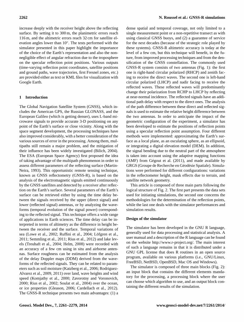
dense spatial and temporal coverage, not only limited to asingle measurement point or a non-repetitive transect as withusing classical GNSS buoys, and (2) a guarantee of servicefor the next decades (because of the strategic role played bythese systems). GNSS-R altimetric accuracy is today at thelevel of a few cm, but this technique will benefit, in the fu-ture, from improved processing techniques and from the den-sification of the GNSS constellation. The commonly usedGNSS-R system consists of two antennas (Fig.1): the firstone is right-hand circular polarized (RHCP) and zenith fac-ing to receive the direct waves. The second one is left-handcircular polarized (LHCP) and nadir facing to receive thereflected waves. These reflected waves will predominantlychange their polarization from RCHP to LHCP by reflectingat near-normal incidence. The reflected signals have an addi-tional path delay with respect to the direct ones. The analysisof the path difference between these direct and reflected sig-nals is used to estimate the relative height difference betweenthe two antennas. In order to anticipate the impact of thegeometric configuration of the experiment, a simulator hasbeen developed to estimate the positions of reflection pointsusing a specular reflection point assumption. Four differentmethods were implemented: approximating the Earth’s sur-face as a local plane, as an osculating sphere, as an ellipsoid,or integrating a digital elevation model (DEM). In addition,the signal bending due to the neutral part of the atmosphereis taken into account using the adaptive mapping functions(AMF) from Gégout et al. (2011), and made available byGRGS (Groupe de Recherche en Géodésie Spatiale). Simula-tions were performed for different configurations: variationsin the reflectometer height, mask effects due to terrain, andsatellite network geometry.

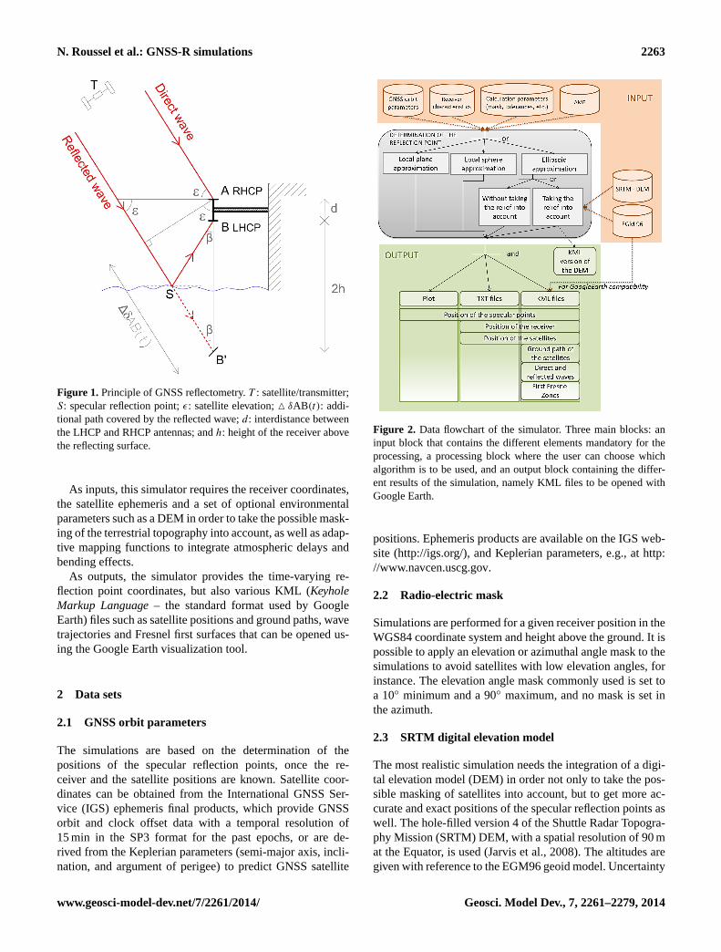
This article is composed of three main parts following thelogical structure of Fig.2. The first part presents the data setsused for initiating simulations, the second one concerns themethodologies for the determination of the reflection points,while the last one deals with the simulator performances andsimulation results.

Design of the simulator

The simulator has been developed in the GNU R language,generally used for data processing and statistical analysis. Auser manual and a description of the R language can be foundon the websitehttp://www.r-project.org/. The main interestof such a language remains in that it is distributed under aGNU GPL license that does R routines in an open sourceprogram, available on various platforms (i.e., GNU/Linux,FreeBSD, NetBSD, OpenBSD, Mac OS and Windows).

The simulator is composed of three main blocks (Fig.2):an input block that contains the different elements manda-tory for the processing, a processing block where the usercan choose which algorithm to use, and an output block con-taining the different results of the simulation.

Geosci. Model Dev., 7, 2261–2279, 2014 www.geosci-model-dev.net/7/2261/2014/

N. Roussel et al.: GNSS-R simulations 2263

Figure 1. Principle of GNSS reflectometry.T : satellite/transmitter;S: specular reflection point;ε: satellite elevation;M δAB(t): addi-tional path covered by the reflected wave;d: interdistance betweenthe LHCP and RHCP antennas; andh: height of the receiver abovethe reflecting surface.

As inputs, this simulator requires the receiver coordinates,the satellite ephemeris and a set of optional environmentalparameters such as a DEM in order to take the possible mask-ing of the terrestrial topography into account, as well as adap-tive mapping functions to integrate atmospheric delays andbending effects.

As outputs, the simulator provides the time-varying re-flection point coordinates, but also various KML (KeyholeMarkup Language– the standard format used by GoogleEarth) files such as satellite positions and ground paths, wavetrajectories and Fresnel first surfaces that can be opened us-ing the Google Earth visualization tool.

2 Data sets

2.1 GNSS orbit parameters

The simulations are based on the determination of thepositions of the specular reflection points, once the re-ceiver and the satellite positions are known. Satellite coor-dinates can be obtained from the International GNSS Ser-vice (IGS) ephemeris final products, which provide GNSSorbit and clock offset data with a temporal resolution of15 min in the SP3 format for the past epochs, or are de-rived from the Keplerian parameters (semi-major axis, incli-nation, and argument of perigee) to predict GNSS satellite

Figure 2. Data flowchart of the simulator. Three main blocks: aninput block that contains the different elements mandatory for theprocessing, a processing block where the user can choose whichalgorithm is to be used, and an output block containing the differ-ent results of the simulation, namely KML files to be opened withGoogle Earth.

positions. Ephemeris products are available on the IGS web-site (http://igs.org/), and Keplerian parameters, e.g., athttp://www.navcen.uscg.gov.

2.2 Radio-electric mask

Simulations are performed for a given receiver position in theWGS84 coordinate system and height above the ground. It ispossible to apply an elevation or azimuthal angle mask to thesimulations to avoid satellites with low elevation angles, forinstance. The elevation angle mask commonly used is set toa 10◦ minimum and a 90◦ maximum, and no mask is set inthe azimuth.

2.3 SRTM digital elevation model

The most realistic simulation needs the integration of a digi-tal elevation model (DEM) in order not only to take the pos-sible masking of satellites into account, but to get more ac-curate and exact positions of the specular reflection points aswell. The hole-filled version 4 of the Shuttle Radar Topogra-phy Mission (SRTM) DEM, with a spatial resolution of 90 mat the Equator, is used (Jarvis et al., 2008). The altitudes aregiven with reference to the EGM96 geoid model. Uncertainty

www.geosci-model-dev.net/7/2261/2014/ Geosci. Model Dev., 7, 2261–2279, 2014

2264 N. Roussel et al.: GNSS-R simulations

in altitude is around 16 m over mountainous areas (Rodriguezet al., 2005). It is made available by files of 5◦ × 5◦ for landareas between 60◦ N and 60◦S by the Consortium for SpatialInformation (CGIAR-CSI;http://srtm.csi.cgiar.org/).

2.4 EGM96 Earth gravitational model

In order to be able to convert between ellipsoidal heights(with respect to the WGS84 ellipsoid) and altitudes (with re-spect to the EGM96 geoid model) when producing KML filesor when integrating a DEM, knowledge of the geoid undula-tion is mandatory. In this study, we interpolate a 15× 15 mingeoid undulation grid file derived from the EGM96 model ina tide-free system released by the US National Geospatial-Intelligence Agency (NGA) EGM development team (http://earth-info.nga.mil/GandG/wgs84/gravitymod/). The error inthe interpolation is lower than 2 cm (NASA and NIMA,1998).

2.5 Adaptive mapping functions

The neutral atmosphere bends the propagation path of theGNSS signal and retards the speed of propagation. The rangebetween the satellite and the tracking site is neither the ge-ometric distance nor the length of the propagation path, butthe radio range of the propagation path (Marini, 1972).

For GNSS-R measurements, the tropospheric effects in-duced by the neutral part of the atmosphere are an impor-tant source of error. Indeed, GNSS-R measurements are oftenmade at low elevation angles, where the bending effects aremaximal. Accurate models have to be used to mitigate sig-nal speed decrease and path bending. Modeling troposphericdelays by calculating the zenith tropospheric delay and ob-taining the slant tropospheric delays with a mapping functionis commonly accepted. New mapping functions were devel-oped in the 2000s (Boehm et al., 2006a; Niell, 2001), and sig-nificantly improve the geodetic positioning. Although mod-ern mapping functions like VMF1 (Boehm et al., 2006b) andGPT2/VMF1 (Lagler et al., 2013) are derived from numer-ical weather models (NWM), most of these mapping func-tions ignore the azimuth dependency, which is usually intro-duced by two horizontal gradient parameters – in the north–south and east–west directions – estimated directly from ob-servations (Chen et al., 1997). More recently, the use of ray-traced delays through NWM directly at observation level hasshown an improvement in geodetic results (Hobiger et al.,2008; Nafisi et al., 2012; Zus et al., 2012). The adaptive map-ping functions (AMF) are designed to fit most of the informa-tion available in NWM – especially the azimuth dependency– preserving the classical mapping function strategy. AMFare thus used to approximate thousands of atmospheric ray-traced delays using a few tens of coefficients with millime-ter accuracy at low elevations (Gégout et al., 2011). AMFhave a classical form, with terms that are functions of the el-evation, but they also include coefficients that depend on the

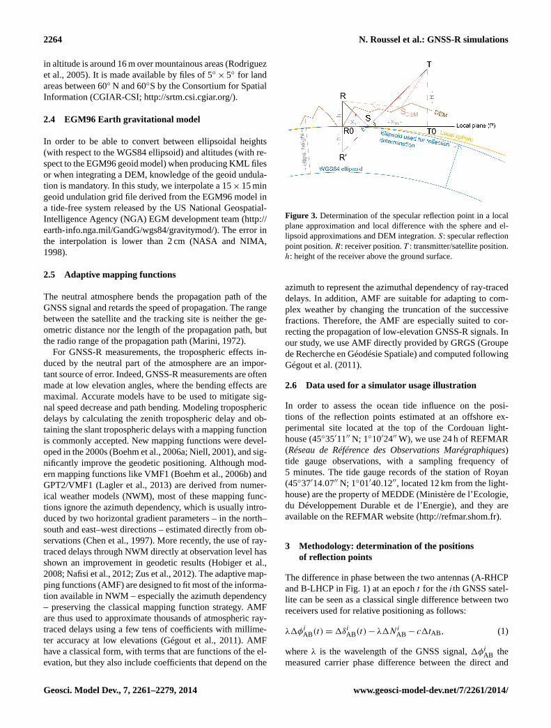
Figure 3. Determination of the specular reflection point in a localplane approximation and local difference with the sphere and el-lipsoid approximations and DEM integration.S: specular reflectionpoint position.R: receiver position.T : transmitter/satellite position.h: height of the receiver above the ground surface.

azimuth to represent the azimuthal dependency of ray-traceddelays. In addition, AMF are suitable for adapting to com-plex weather by changing the truncation of the successivefractions. Therefore, the AMF are especially suited to cor-recting the propagation of low-elevation GNSS-R signals. Inour study, we use AMF directly provided by GRGS (Groupede Recherche en Géodésie Spatiale) and computed followingGégout et al. (2011).

2.6 Data used for a simulator usage illustration

In order to assess the ocean tide influence on the posi-tions of the reflection points estimated at an offshore ex-perimental site located at the top of the Cordouan light-house (45◦35′11′′ N; 1◦10′24′′ W), we use 24 h of REFMAR(Réseau de Référence des Observations Marégraphiques)tide gauge observations, with a sampling frequency of5 minutes. The tide gauge records of the station of Royan(45◦37′14.07′′ N; 1◦01′40.12′′, located 12 km from the light-house) are the property of MEDDE (Ministère de l’Ecologie,du Développement Durable et de l’Energie), and they areavailable on the REFMAR website (http://refmar.shom.fr).

3 Methodology: determination of the positionsof reflection points

The difference in phase between the two antennas (A-RHCPand B-LHCP in Fig.1) at an epocht for theith GNSS satel-lite can be seen as a classical single difference between tworeceivers used for relative positioning as follows:

λ1φiAB(t) = 1δi

AB(t) − λ1N iAB − c1tAB, (1)

whereλ is the wavelength of the GNSS signal,1φiAB the

measured carrier phase difference between the direct and

Geosci. Model Dev., 7, 2261–2279, 2014 www.geosci-model-dev.net/7/2261/2014/

N. Roussel et al.: GNSS-R simulations 2265

received signals expressed in cycles,1δiAB the difference in

distance between the direct and received signals,1N iAB is

the difference of phase ambiguity between the direct and re-ceived signals,c the speed of light in a vacuum, and1tAB thereceiver clock bias difference. As the baseline between thetwo receivers is short (a few cm to a few tenths of cm), andin the case of low altitude of the receivers, both troposphericand ionospheric effects are neglected due to the spatial res-olution of the current atmospheric and ionospheric models.Besides, when both antennas are connected to the same re-ceiver, the receiver clock bias difference is also cancelled out.In this study, we only consider the difference in distance be-tween direct and reflected signals, as illustrated in Fig.1.

The processing block contains four algorithms for deter-mining the positions of the specular reflection points: the firstconsidering the Earth as a local plane in the vicinity of the re-flection point, the second as an osculating sphere, the third asan ellipsoid that corresponds to the WGS84 ellipsoid, whichhas been expanded until the ellipsoid height of the receiverequals the height of the receiver above the reflecting surface(see Sect.3.3), and the last one uses the ellipsoid approx-imation, but takes the Earth’s topography into account: seeFig.3. Comparisons between the different approximations ofthe Earth’s shape will be performed in Sect.4.1.

All of them are based on iterative approaches to solvingthe Snell–Descartes law for reflection: the unique assumptionis that the angle of incidence is equal to the angle of reflec-tion on a plane interface separating two half-space media (alocally planar approximation is adopted when the surface isnot planar everywhere). In the plane, sphere and ellipsoid ap-proximations, the specular reflection point of a given satelliteis contained within the plane defined by the satellite, the re-ceiver and the center of the Earth. With regards to the DEMintegration, reflection can occur everywhere. In order to beable to compare the specular reflection point positions ob-tained by integrating a DEM, and to simplify the problem, wewill only consider the reflections occurring within the plane,even while integrating a DEM.

3.1 Local plane reflection approximation

Refering to Fig.3, let us consider the projection of thereceiverR0 on the osculating sphere approximation (seeSect.3.2). We define the local planeP as the plane tangent tothe sphere atR0. LetT 0 be the projection of the satellite onP andR′ the symmetry ofR0 relative toP . We look for thepositions of the specular reflection points onP . Consideringthe Thales theorem in trianglesR′SR0 andST T 0, we have(see Fig.3)

XS

(XT 0 − XS)=

h

H. (2)

Thus,

XS =hXT 0

H + h. (3)

3.2 Local sphere reflection approximation

The model we consider is an osculating sphere. Its radial di-rection coincides with the ellipsoidal normal, and its centeris set at an ellipsoidal height equal to the negative value ofthe Gaussian radius of curvature defined as

rE =a′2b′

a′2cos2(ϕ) + b′2sin2(ϕ), (4)

with ϕ the latitude of the receiver, anda′ andb′ the semi-major and semi-minor axes of the modified ellipsoid (seeSect.3.3). Please refer to Nievinski and Santos (2010) forfurther information on the different approximations of theEarth, particularly on the osculating sphere.

J. Kostelecky and C. Wagner already suggested an algo-rithm to retrieve the specular reflection point positions byapproximating the Earth as a sphere (Kostelecky et al., 2005;Wagner and Klokocnik, 2003). Their algorithm is based onan optimized iterative scheme that is equivalent to makingthe position of a fictive specular point vary until verifyingthe first law of Snell and Descartes. A similar approach willbe used in this paper in Sect.3.3 with the ellipsoid approxi-mation. Here, we chose to adopt a more analytical algorithm,first proposed by Helm (2008). In order to validate this al-gorithm, comparisons between it and the iterative one devel-oped for the ellipsoid approach will be performed, by settingthe minor and major axes of the ellipsoid equal to the sphereradius (see Sect.4.2.1).

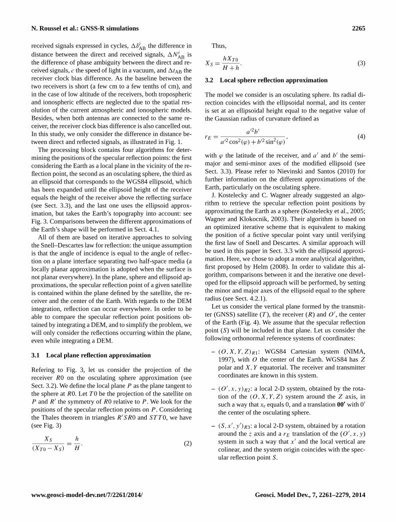
Let us consider the vertical plane formed by the transmit-ter (GNSS) satellite (T ), the receiver (R) andO ′, the centerof the Earth (Fig.4). We assume that the specular reflectionpoint (S) will be included in that plane. Let us consider thefollowing orthonormal reference systems of coordinates:

– (O,X,Y,Z)R1: WGS84 Cartesian system (NIMA ,1997), with O the center of the Earth. WGS84 hasZ

polar andX,Y equatorial. The receiver and transmittercoordinates are known in this system.

– (O ′,x,y)R2: a local 2-D system, obtained by the rota-tion of the (O,X,Y,Z) system around theZ axis, insuch a way thatxr equals 0, and a translation00′ with 0′

the center of the osculating sphere.

– (S,x′,y′)R3: a local 2-D system, obtained by a rotationaround thez axis and arE translation of the (O ′,x,y)system in such a way thatx′ and the local vertical arecolinear, and the system origin coincides with the spec-ular reflection pointS.

www.geosci-model-dev.net/7/2261/2014/ Geosci. Model Dev., 7, 2261–2279, 2014

2266 N. Roussel et al.: GNSS-R simulations

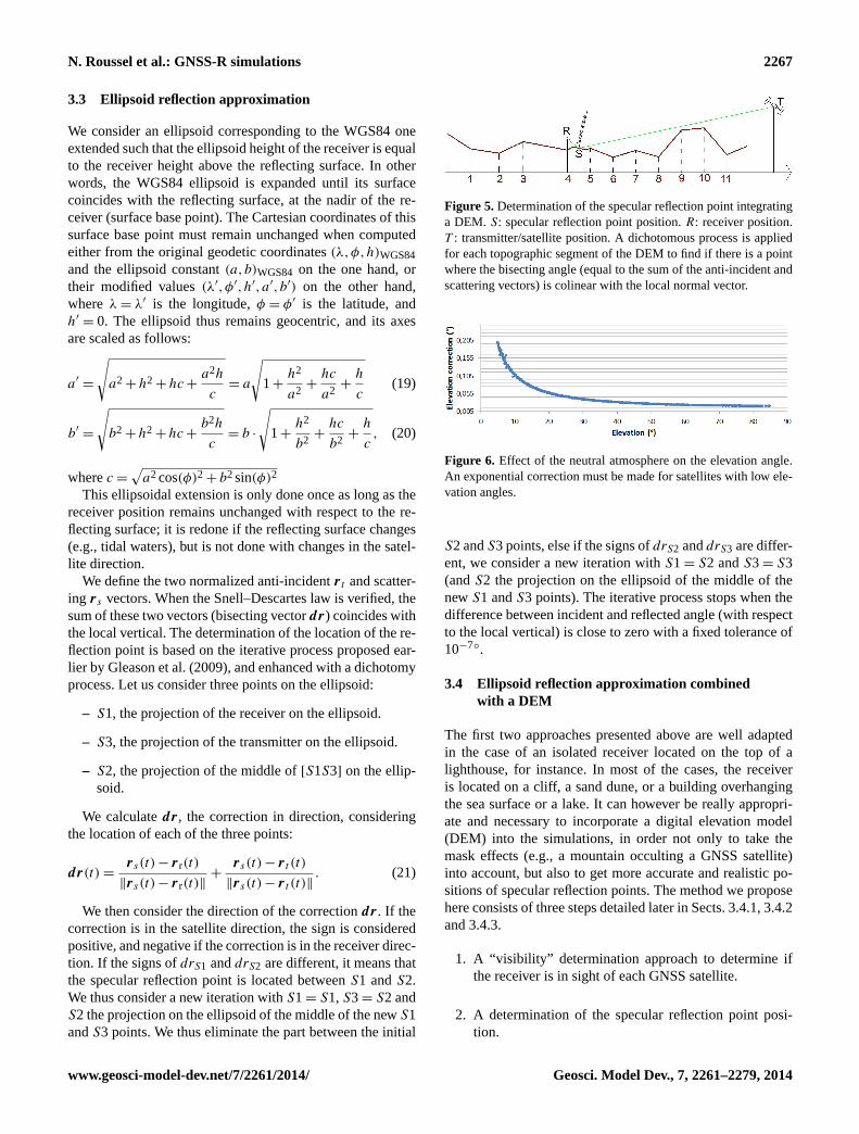
Figure 4. Local osculating sphere approximation: the three dif-ferent reference systems of coordinates.S: specular reflectionpoint position.R: receiver position.T : transmitter/satellite posi-tion. (0,X,Y,Z)R1: WGS84 Cartesian system.(0′,x,y)R2: local2-D system, centred on the center of the osculating sphere, obtainedby the rotation of theR1 system around theZ axis, in such a waythat xr equals 0.(S,x′,y′)R3: a local 2-D system, obtained by arotation around thez axis and arR translation of the R2 system insuch a way thatx′ and the local vertical are colinear and the systemorigin coincides with the specular reflection pointS.

If H is the height of the receiver above the ground, theposition of the receiver is

r r =

(xryr

)R2

=

(0

rE + H

)R2

, (5)

with rE the Gaussian radius of curvature at the latitude of thereceiverϕr.

The position of the GNSS satellite transmitter consideringε the elevation angle of the satellite (considering the zenithangle reckoned from the ellipsoidal normal direction) andτ

the angleR̂T O ′ is given by

rt =

(xt

yt

)R2

=

(rt cos(ε + τ)

rt sin(ε + τ)

)R2

. (6)

Using the trigonometric sine formula in theR−T −0′ tri-angle,

sin(π2 + ε)

rt=

sin(τ )

rE + H, (7)

we finally obtain

(xt

yt

)R2

=

rt cos(ε)√

1−(rE+H)2

r2t

cos2(ε)

−(rE + H)sin(ε)cos(ε)

rt sin(ε)√

1−(rE+H)2

r2t

cos2(ε)

−(rE + H)cos2(ε)

R2

. (8)

The Snell–Descartes law for reflection can be expressed asthe ratios of the coordinates of the receiver and the transmit-ter in (S,x′,y′):

x′t

y′t

=x′

r

y′r. (9)

The coordinates inR3 can be derived from the coordinatesin R2 from(

x′

y′

)R3

=

(cos(γ ) sin(γ )

−sin(γ ) cos(γ ))

)R3

(x

y

)R2

−

(re0

)R3

, (10)

where γ is the rotation angle between the two systems(Fig. 4). Eq. (9) thus becomes

2(xtxr − ytyr)sin(γ )cos(γ )

− (xtyr + ytxr)(cos2(γ ) − sin2(γ ))

− rE(xt + xr)sin(γ ) + re(yt + yr)cos(γ ) = 0 (11)

Following (Helm, 2008), we proceed to the substitutiont = tan( γ

2 ), and Eq. (11) becomes

2(xtxr − ytyr)2t

1+ t2

1− t2

1+ t2− xtyr((

1− t2

1+ t2)2

−(2t

1+ t2)2) − rE

2t

1+ t2(xt + xr)

+rE1− t2

1+ t2(yt + yr) = 0. (12)

This finally becomes

c4t4+ c3t

3+ c2t

2+ c11

t + c0 = 0, (13)

with

c0 = (xtyr + ytxr) − rE(yt + yr) (14)

c1 = −4(xtxr − ytyr) + 2rE(xt + xr) (15)

c2 = −6(xtyr + yrxr) (16)

c3 = 4(xtxr − ytyr) + 2rE(xt + xr) (17)

c4 = (xtyr + ytxr) + rE(yt + yr). (18)

Equation (13) is solved to determine the roots of thispolynomial using an iterative scheme based on the Newtonmethod (Nocedal et al., 2006).

Geosci. Model Dev., 7, 2261–2279, 2014 www.geosci-model-dev.net/7/2261/2014/

N. Roussel et al.: GNSS-R simulations 2267

3.3 Ellipsoid reflection approximation

We consider an ellipsoid corresponding to the WGS84 oneextended such that the ellipsoid height of the receiver is equalto the receiver height above the reflecting surface. In otherwords, the WGS84 ellipsoid is expanded until its surfacecoincides with the reflecting surface, at the nadir of the re-ceiver (surface base point). The Cartesian coordinates of thissurface base point must remain unchanged when computedeither from the original geodetic coordinates(λ,φ,h)WGS84and the ellipsoid constant(a,b)WGS84 on the one hand, ortheir modified values(λ′,φ′,h′,a′,b′) on the other hand,where λ = λ′ is the longitude,φ = φ′ is the latitude, andh′

= 0. The ellipsoid thus remains geocentric, and its axesare scaled as follows:

a′=

√a2 + h2 + hc +

a2h

c= a

√1+

h2

a2+

hc

a2+

h

c(19)

b′=

√b2 + h2 + hc +

b2h

c= b ·

√1+

h2

b2+

hc

b2+

h

c, (20)

wherec =

√a2cos(φ)2 + b2sin(φ)2

This ellipsoidal extension is only done once as long as thereceiver position remains unchanged with respect to the re-flecting surface; it is redone if the reflecting surface changes(e.g., tidal waters), but is not done with changes in the satel-lite direction.

We define the two normalized anti-incidentr t and scatter-ing rs vectors. When the Snell–Descartes law is verified, thesum of these two vectors (bisecting vectordr) coincides withthe local vertical. The determination of the location of the re-flection point is based on the iterative process proposed ear-lier by Gleason et al. (2009), and enhanced with a dichotomyprocess. Let us consider three points on the ellipsoid:

– S1, the projection of the receiver on the ellipsoid.

– S3, the projection of the transmitter on the ellipsoid.

– S2, the projection of the middle of[S1S3] on the ellip-soid.

We calculatedr, the correction in direction, consideringthe location of each of the three points:

dr(t) =rs(t) − r r(t)

‖rs(t) − r r(t)‖+

rs(t) − r t (t)

‖rs(t) − r t (t)‖. (21)

We then consider the direction of the correctiondr. If thecorrection is in the satellite direction, the sign is consideredpositive, and negative if the correction is in the receiver direc-tion. If the signs ofdrS1 anddrS2 are different, it means thatthe specular reflection point is located betweenS1 andS2.We thus consider a new iteration withS1 = S1,S3 = S2 andS2 the projection on the ellipsoid of the middle of the newS1andS3 points. We thus eliminate the part between the initial

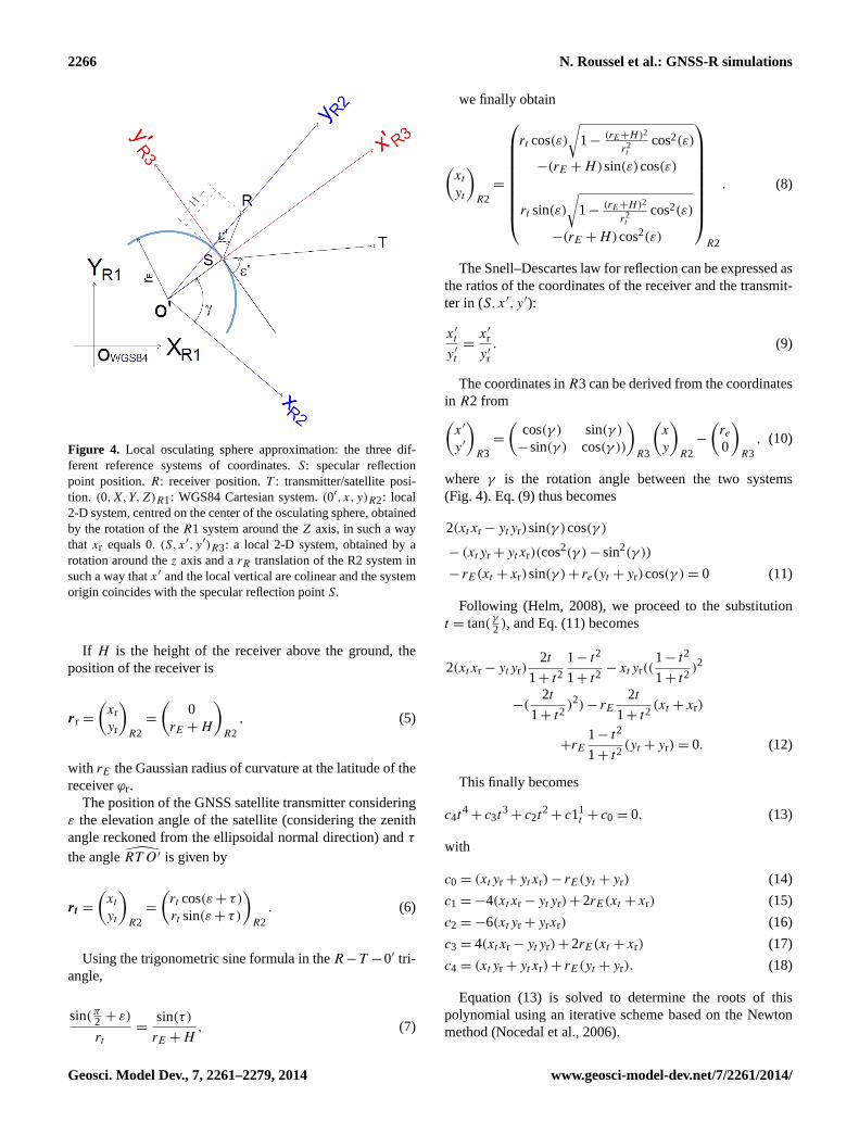
Figure 5. Determination of the specular reflection point integratinga DEM. S: specular reflection point position.R: receiver position.T : transmitter/satellite position. A dichotomous process is appliedfor each topographic segment of the DEM to find if there is a pointwhere the bisecting angle (equal to the sum of the anti-incident andscattering vectors) is colinear with the local normal vector.

Figure 6. Effect of the neutral atmosphere on the elevation angle.An exponential correction must be made for satellites with low ele-vation angles.

S2 andS3 points, else if the signs ofdrS2 anddrS3 are differ-ent, we consider a new iteration withS1 = S2 andS3 = S3(andS2 the projection on the ellipsoid of the middle of thenewS1 andS3 points). The iterative process stops when thedifference between incident and reflected angle (with respectto the local vertical) is close to zero with a fixed tolerance of10−7◦.

3.4 Ellipsoid reflection approximation combinedwith a DEM

The first two approaches presented above are well adaptedin the case of an isolated receiver located on the top of alighthouse, for instance. In most of the cases, the receiveris located on a cliff, a sand dune, or a building overhangingthe sea surface or a lake. It can however be really appropri-ate and necessary to incorporate a digital elevation model(DEM) into the simulations, in order not only to take themask effects (e.g., a mountain occulting a GNSS satellite)into account, but also to get more accurate and realistic po-sitions of specular reflection points. The method we proposehere consists of three steps detailed later in Sects.3.4.1, 3.4.2and3.4.3.

1. A “visibility” determination approach to determine ifthe receiver is in sight of each GNSS satellite.

2. A determination of the specular reflection point posi-tion.

www.geosci-model-dev.net/7/2261/2014/ Geosci. Model Dev., 7, 2261–2279, 2014

2268 N. Roussel et al.: GNSS-R simulations

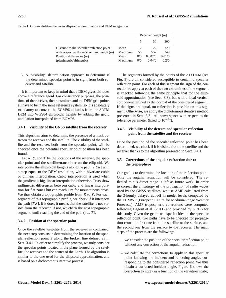
Table 1.Cross-validation between ellipsoid approximation and DEM integration.

Receiver height (m)

5 50 300

Distance to the specular reflection point Mean 12 122 729with respect to the receiver: arc length (m) Maximum 56 557 3349Position differences (m) Mean 0/0 0.002/0 0.01/0(planimetric/altimetric) Maximum 0/0 0.04/0 0.2/0

3. A “visibility” determination approach to determine ifthe determined specular point is in sight from both re-ceiver and satellite.

It is important to keep in mind that a DEM gives altitudesabove a reference geoid. For consistency purposes, the posi-tions of the receiver, the transmitter, and the DEM grid pointsall have to be in the same reference system, so it is absolutelymandatory to convert the EGM96 altitudes from the SRTMDEM into WGS84 ellipsoidal heights by adding the geoidundulation interpolated from EGM96.

3.4.1 Visibility of the GNSS satellite from the receiver

This algorithm aims to determine the presence of a mask be-tween the receiver and the satellite. The visibility of the satel-lite and the receiver, both from the specular point, will bechecked once the potential specular point position has beenfound.

Let R, S, andT be the locations of the receiver, the spec-ular point and the satellite/transmitter on the ellipsoid. Weinterpolate the ellipsoidal heights along the path[T SR] witha step equal to the DEM resolution, with a bivariate cubicor bilinear interpolation. Cubic interpolation is used whenthe gradient is big, linear interpolation otherwise. Tests showmillimetric differences between cubic and linear interpola-tion for flat zones but can reach 1 m for mountainous areas.We thus obtain a topographic profile fromR to T . For eachsegment of this topographic profile, we check if it intersectsthe path[T R]. If it does, it means that the satellite is not vis-ible from the receiver. If not, we check the next topographicsegment, until reaching the end of the path (i.e.,T ).

3.4.2 Position of the specular point

Once the satellite visibility from the receiver is confirmed,the next step consists in determining the location of the spec-ular reflection pointS along the broken line defined as inSect.3.4.1. In order to simplify the process, we only considerthe specular points located in the plane formed by the satel-lite, the receiver and the center of the Earth. The algorithm issimilar to the one used for the ellipsoid approximation, andis based on a dichotomous iterative process.

The segments formed by the points of the 2-D DEM (seeFig. 5) are all considered susceptible to contain a specularreflection point. For each of this segment the sign of the cor-rection to apply at each of the two extremities of the segmentis checked following the same principle that for the ellip-soid approximation (see Sect.3.3), but with a local verticalcomponent defined as the normal of the considered segment.If the signs are equal, no reflection is possible on this seg-ment. Otherwise, we apply the dichotomous iterative methodpresented in Sect.3.3 until convergence with respect to thetolerance parameter (fixed to 10−7◦).

3.4.3 Visibility of the determined specular reflectionpoint from the satellite and the receiver

Once the position of the specular reflection point has beendetermined, we check if it is visible from the satellite and thereceiver thanks to the algorithm presented in Sect.3.4.1.

3.5 Corrections of the angular refraction due tothe troposphere

Our goal is to determine the location of the reflection point.Only the angular refraction will be considered. The re-flected minus direct range is left as future work. In orderto correct the anisotropy of the propagation of radio wavesused by the GNSS satellites, we use AMF calculated fromthe 3-hourly delayed cut-off in model levels computed bythe ECMWF (European Centre for Medium-Range WeatherForecasts). AMF tropospheric corrections were computedfollowing Gegout et al. (2011) and provided by GRGS forthis study. Given the geometric specificities of the specularreflection point, two paths have to be checked for propaga-tion error: the first one from the satellite to the surface, andthe second one from the surface to the receiver. The mainsteps of the process are the following:

– we consider the position of the specular reflection pointwithout any correction of the angular refraction;

– we calculate the corrections to apply to this specularpoint knowing the incident and reflecting angles cor-responding to the considered reflection point. We thusobtain a corrected incident angle. Figure6 shows thecorrection to apply as a function of the elevation angle;

Geosci. Model Dev., 7, 2261–2279, 2014 www.geosci-model-dev.net/7/2261/2014/

N. Roussel et al.: GNSS-R simulations 2269

– from the corrected incident angle, a corrected positionof the specular point is calculated, making the reflectingangle equal to the corrected incident angle;

– with the new position of the specular point, and to reacha better accuracy of the point position, a second iterationis performed by computing the corrections to apply tothis new incident angle.

3.5.1 Correction of the satellite-surface path

First and foremost, the parallax problem for the wave emit-ted by a known GNSS satellite is solved. At first sight, theposition of the specular reflection point calculated withoutany correction of the angular refraction is considered, givenby the algorithm approximating the Earth’s shape as a spheregiven in Sect.3.2. We use here AMF calculated from the pro-jection of the receiver on the surface, considering that theAMF planimetric variations are negligible for ground-basedobservations (i.e., we consider that we can use the same AMFfor every specular reflection points, which is valid only ifthe specular reflection points are less than few tens of kmfrom the receiver and that the specular points lie on an equal-height surface). We thus obtain the corrected incident an-gle of the incident wave. Considering the law of Snell andDescartes, the reflecting angle must be equal to the correctedincident angle, for the specular reflection point position.

3.5.2 Correction of the surface-receiver path

The aim here is to adjust the surface-receiver path to accom-modate the consequences of angular refraction. With the cor-rected reflection angle, we can deduce the corrected geomet-ric distance between the reflection point and the receiver, thistime using AMF calculated from the receiver, assuming thatthe AMF altimetric variations are non-negligible (i.e., thepart of the troposphere corresponding to the receiver heightwill have a non-negligible impact on the AMF). Consider-ing the corrected geometric distance between the reflectionpoint and the receiver, the corrected position of the reflectionpoint is obviously determined. It is indeed obtained as theintersection of a circle whose radius is equal to the correctgeometric distance, with the surface of the Earth assimilatedas a sphere, an ellipsoid, or with a DEM, depending on whichapproximation of the Earth is taken into account.

The whole process is iterated a second time to reach a bet-ter accuracy of the reflection point location. In fact, the firstcorrections were not perfectly exact, since they were com-puted from an initially false reflection point location, andthe second iteration brings the point closer to the true loca-tion. More iterations are useless (corrections to apply are notsignificant). Figure6 shows an example of elevation correc-tions to apply as functions of the satellite elevations. This fig-ure has been computed from simulations done on a receiver

placed on the Lake Geneva shore (46◦24′30′′ N, 6◦43′6′′ E;471 m); see Sect.4.1.

3.6 Footprint size of the reflected signal

The power of the received signal is mostly due to coherentreflection, and most of the scattering comes from the firstFresnel zone (Beckmann and Spizzichino, 1987). The firstFresnel zone can be described as an ellipse of a semi-minoraxis (ra) and a semi-major axis (rb) equal to (Larson andNievinski, 2013)

rb =

√λh

sin(ε′)+

(λ

2sin(ε′)

)2

(22)

ra =b

sin(ε′), (23)

with λ the wavelength (m),h the receiver height (m) andε′

the satellite elevation seen from the specular reflection point(rad) (i.e., corresponding to the reflection angle).

4 Simulator performance and results

4.1 Simulation case studies

Simulations and tests of parameters have been performed ontwo main sites:

– the Cordouan lighthouse (45◦35′11′′ N; 1◦10′24′′ W), inthe Gironde estuary, France. This lighthouse is about60 m high, and it is surrounded by the sea.

– the shore of Lake Geneva (46◦24′30′′ N; 6◦43′6′′ E).This site is hidden by mountains in the south (ortho-metric altitude of up to 2000 m), and overlooks the lakein the north (orthometric altitude of 370 m).

For both sites, precise GPS and GLONASS ephemeris ata 15 min time sampling come from IGS standard products(known as “SP3 orbit”).

4.2 Validation of the surface models

Simulations were performed in the case of the Lake Genevashore, for a 24 h experiment, on 4 October 2012.

4.2.1 Cross-validation between sphere andellipsoid approximations

Local sphere and ellipsoid approximation algorithms havebeen compared by putting the ellipsoid semi- major and mi-nor axis equal to the sphere radius. Planimetric and altimetricdifferences between both are below 6×10−5 m for a receiverheight above reflecting surface between 5 and 300 m and arethen negligible. The two algorithms we compare are com-pletely different: the first is analytical and the second is basedon a iterative scheme and both results are very similar, whichconfirms their validity.

www.geosci-model-dev.net/7/2261/2014/ Geosci. Model Dev., 7, 2261–2279, 2014

2270 N. Roussel et al.: GNSS-R simulations

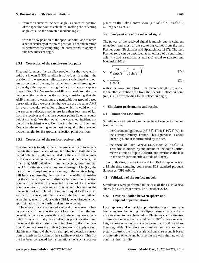
Figure 7. Positions of the specular reflection points and first Fresnel zones for one week of simulation on the Cordouan lighthouse with a15 min sampling rate (i.e., satellite positions actualized every 15 min). Only GPS satellites with elevation angles greater than 5◦ have beenconsidered. Note the gap in the northerly direction.

Figure 8. First Fresnel zones and some direct and reflected waves displaying the 24 h Cordouan lighthouse simulation with the GPS constel-lation.

4.2.2 Cross-validation between ellipsoid approximationand DEM integration

The algorithm integrating a DEM has been compared to theellipsoid approximation algorithm by using a flat DEM as in-put (i.e., a DEM with orthometric altitude equal to the geoidundulation). Results for satellite elevation angles above 5◦

are presented in Table1.

As we can see in Table1, planimetric and altimetric meandifferences are subcentimetric for a 5 and 50 m receiverheight and centimetric for a 300 m receiver height. How-ever, some punctual planimetric differences reach 20 cm inthe worst conditions (reflection occurring at 3449 m from thereceiver corresponding to a satellite with a low elevation an-gle), which can be explained with the chosen tolerance pa-rameters but mainly because due to the DEM resolution, thealgorithm taking a DEM into account approximating the el-lipsoid as a broken straight line, causing inaccuracies. For a

Geosci. Model Dev., 7, 2261–2279, 2014 www.geosci-model-dev.net/7/2261/2014/

N. Roussel et al.: GNSS-R simulations 2271

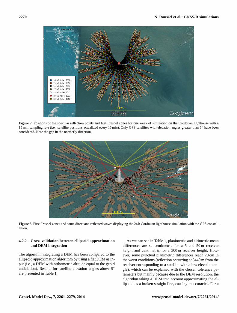
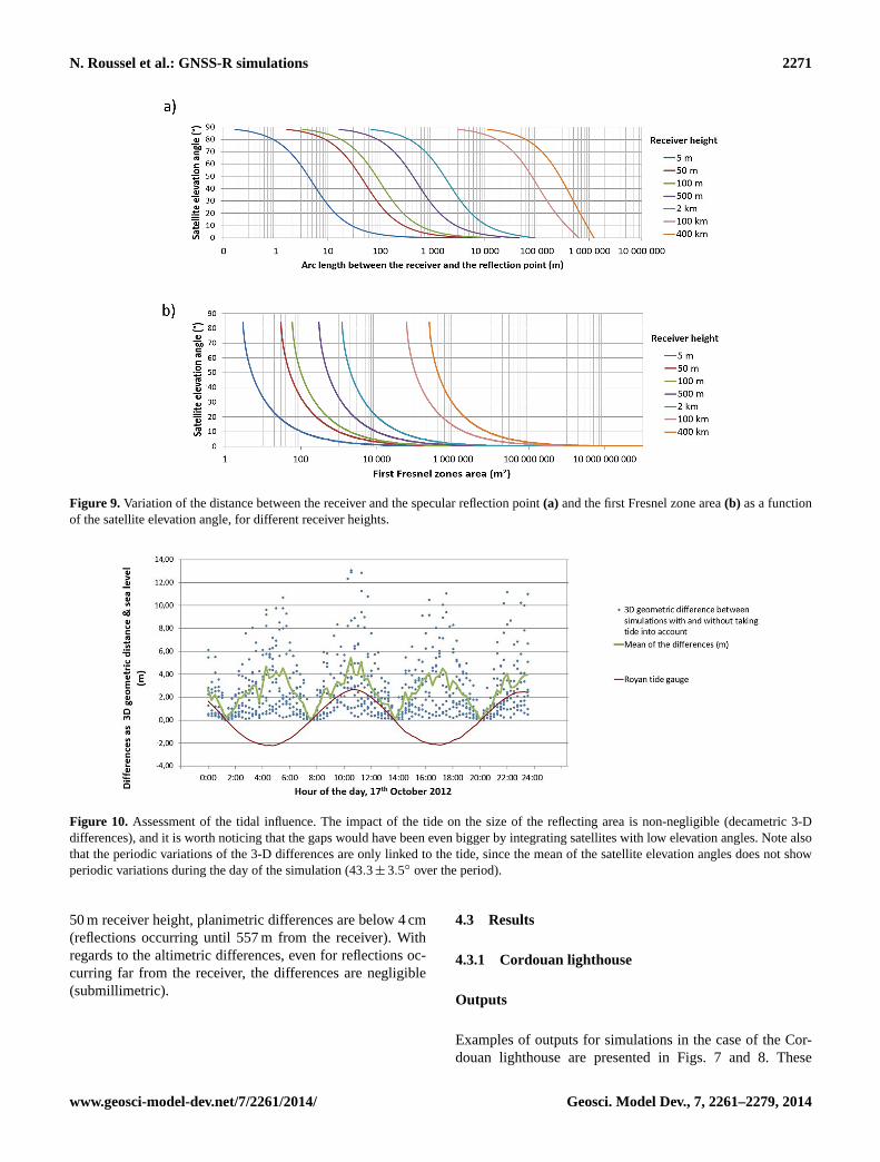
Figure 9. Variation of the distance between the receiver and the specular reflection point(a) and the first Fresnel zone area(b) as a functionof the satellite elevation angle, for different receiver heights.

Figure 10. Assessment of the tidal influence. The impact of the tide on the size of the reflecting area is non-negligible (decametric 3-Ddifferences), and it is worth noticing that the gaps would have been even bigger by integrating satellites with low elevation angles. Note alsothat the periodic variations of the 3-D differences are only linked to the tide, since the mean of the satellite elevation angles does not showperiodic variations during the day of the simulation (43.3± 3.5◦ over the period).

50 m receiver height, planimetric differences are below 4 cm(reflections occurring until 557 m from the receiver). Withregards to the altimetric differences, even for reflections oc-curring far from the receiver, the differences are negligible(submillimetric).

4.3 Results

4.3.1 Cordouan lighthouse

Outputs

Examples of outputs for simulations in the case of the Cor-douan lighthouse are presented in Figs.7 and 8. These

www.geosci-model-dev.net/7/2261/2014/ Geosci. Model Dev., 7, 2261–2279, 2014

2272 N. Roussel et al.: GNSS-R simulations

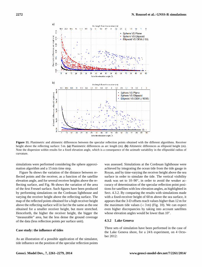
Figure 11. Planimetric and altimetric differences between the specular reflection points obtained with the different algorithms. Receiverheight above the reflecting surface: 5 m.(a) Planimetric differences as arc length (m).(b) Altimetric differences as ellipsoid height (m).Note the dispersion within results for a fixed elevation angle, which is a consequence of the azimuth variability in the ellipsoidal radius ofcurvature.

simulations were performed considering the sphere approxi-mation algorithm and a 15 min time step.

Figure9a shows the variation of the distance between re-flected points and the receiver, as a function of the satelliteelevation angle, and for several receiver heights above the re-flecting surface, and Fig.9b shows the variation of the areaof the first Fresnel surface. Such figures have been producedby performing simulations on the Cordouan lighthouse andvarying the receiver height above the reflecting surface. Themap of the reflected points obtained for a high receiver heightabove the reflecting surface will in fact be the same as the oneobtained for a smaller receiver height, but more stretched.Henceforth, the higher the receiver height, the bigger the“measurable” area, but the less dense the ground coverageof the data (less reflection points per surface unit).

Case study: the influence of tides

As an illustration of a possible application of the simulator,tide influence on the position of the specular reflection points

was assessed. Simulations at the Cordouan lighthouse wereachieved by integrating the ocean tide from the tide gauge inRoyan, and by time-varying the receiver height above the seasurface in order to simulate the tide. The vertical visibilitymask was set to 10–90◦, in order to avoid the weaker ac-curacy of determination of the specular reflection point posi-tions for satellites with low elevation angles, as highlighted inSect.4.3.2. By comparing the results with simulations madewith a fixed-receiver height of 60 m above the sea surface, itappears that the 3-D offsets reach values higher than 12 m forthe maximum tide values (< 3 m) (Fig. 10). We can expecteven higher discrepancies by taking into account satelliteswhose elevation angles would be lower than 10◦.

4.3.2 Lake Geneva

Three sets of simulation have been performed in the case ofthe Lake Geneva shore, for a 24 h experiment, on 4 Octo-ber 2012:

Geosci. Model Dev., 7, 2261–2279, 2014 www.geosci-model-dev.net/7/2261/2014/

N. Roussel et al.: GNSS-R simulations 2273

Table 2.Maximum differences between the positions of the specular reflection points obtained with the different algorithms and for differentreceiver heights above the reflecting surface. For each cell of this table, the first number is the result obtained with the minimum satelliteelevation angle set to 5◦, and the second number is the result obtained with the minimum satellite elevation angle set to 10◦.

Receiver Differences Sphere vs. Plane sphere vs. ellipsoid Ellipsoid vs. DEMheight (m) (m)

Arc length 0.015/ 0.003 0.108/ 0.054 14.594/ 4.4175 Ellipsoid height 0/ 0 0/ 0 1.500/ 1.500

3-D geometric distance 0.011/ 0.002 0.084/ 0.044 10.261/ 3.383

Arc length 1.163/ 0.142 1.081/ 0.536 1226.606/ 42.98250 Ellipsoid height 0.025/ 0.006 0/ 0 84.363/ 15.002

3-D geometric distance 0.823/ 0.107 0.837/ 0.440 1235.834/ 43.755

Arc length 41.127/ 5.043 6.438/ 3.215 5429.975/ 5429.975300 Ellipsoid height 0.885/ 0.222 0.001/ 0 897.785/ 897.785

3-D geometric distance 29.092/ 3.769 4.994/ 2.634 5461.230/ 5461.230

Figure 12. Planimetric and altimetric differences between the specular reflection points obtained with the different algorithms. Receiverheight above the reflecting surface: 50 m.(a) Planimetric differences as arc length (m).(b) Altimetric differences as ellipsoid height (m).Note the dispersion within results for a fixed elevation angle, which is a consequence of the azimuth variability in the ellipsoidal radius ofcurvature.

www.geosci-model-dev.net/7/2261/2014/ Geosci. Model Dev., 7, 2261–2279, 2014

2274 N. Roussel et al.: GNSS-R simulations

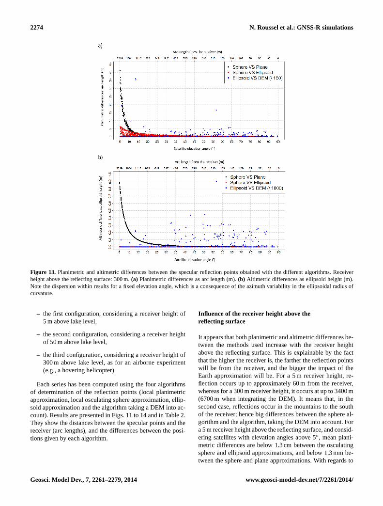
Figure 13. Planimetric and altimetric differences between the specular reflection points obtained with the different algorithms. Receiverheight above the reflecting surface: 300 m.(a) Planimetric differences as arc length (m).(b) Altimetric differences as ellipsoid height (m).Note the dispersion within results for a fixed elevation angle, which is a consequence of the azimuth variability in the ellipsoidal radius ofcurvature.

– the first configuration, considering a receiver height of5 m above lake level,

– the second configuration, considering a receiver heightof 50 m above lake level,

– the third configuration, considering a receiver height of300 m above lake level, as for an airborne experiment(e.g., a hovering helicopter).

Each series has been computed using the four algorithmsof determination of the reflection points (local planimetricapproximation, local osculating sphere approximation, ellip-soid approximation and the algorithm taking a DEM into ac-count). Results are presented in Figs.11to 14and in Table2.They show the distances between the specular points and thereceiver (arc lengths), and the differences between the posi-tions given by each algorithm.

Influence of the receiver height above thereflecting surface

It appears that both planimetric and altimetric differences be-tween the methods used increase with the receiver heightabove the reflecting surface. This is explainable by the factthat the higher the receiver is, the farther the reflection pointswill be from the receiver, and the bigger the impact of theEarth approximation will be. For a 5 m receiver height, re-flection occurs up to approximately 60 m from the receiver,whereas for a 300 m receiver height, it occurs at up to 3400 m(6700 m when integrating the DEM). It means that, in thesecond case, reflections occur in the mountains to the southof the receiver; hence big differences between the sphere al-gorithm and the algorithm, taking the DEM into account. Fora 5 m receiver height above the reflecting surface, and consid-ering satellites with elevation angles above 5◦, mean plani-metric differences are below 1.3 cm between the osculatingsphere and ellipsoid approximations, and below 1.3 mm be-tween the sphere and plane approximations. With regards to

Geosci. Model Dev., 7, 2261–2279, 2014 www.geosci-model-dev.net/7/2261/2014/

N. Roussel et al.: GNSS-R simulations 2275

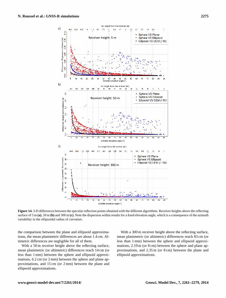
Figure 14.3-D differences between the specular reflection points obtained with the different algorithms. Receiver heights above the reflectingsurface of 5 m(a), 50 m(b) and 300 m(c). Note the dispersion within results for a fixed elevation angle, which is a consequence of the azimuthvariability in the ellipsoidal radius of curvature.

the comparison between the plane and ellipsoid approxima-tions, the mean planimetric differences are about 1.4 cm. Al-timetric differences are negligible for all of them.

With a 50 m receiver height above the reflecting surface,mean planimetric (or altimetric) differences reach 14 cm (orless than 1 mm) between the sphere and ellipsoid approxi-mations, 6.2 cm (or 2 mm) between the sphere and plane ap-proximations, and 15 cm (or 2 mm) between the plane andellipsoid approximations.

With a 300 m receiver height above the reflecting surface,mean planimetric (or altimetric) differences reach 83 cm (orless than 1 mm) between the sphere and ellipsoid approxi-mations, 2.19 m (or 8 cm) between the sphere and plane ap-proximations, and 2.35 m (or 8 cm) between the plane andellipsoid approximations.

www.geosci-model-dev.net/7/2261/2014/ Geosci. Model Dev., 7, 2261–2279, 2014

2276 N. Roussel et al.: GNSS-R simulations

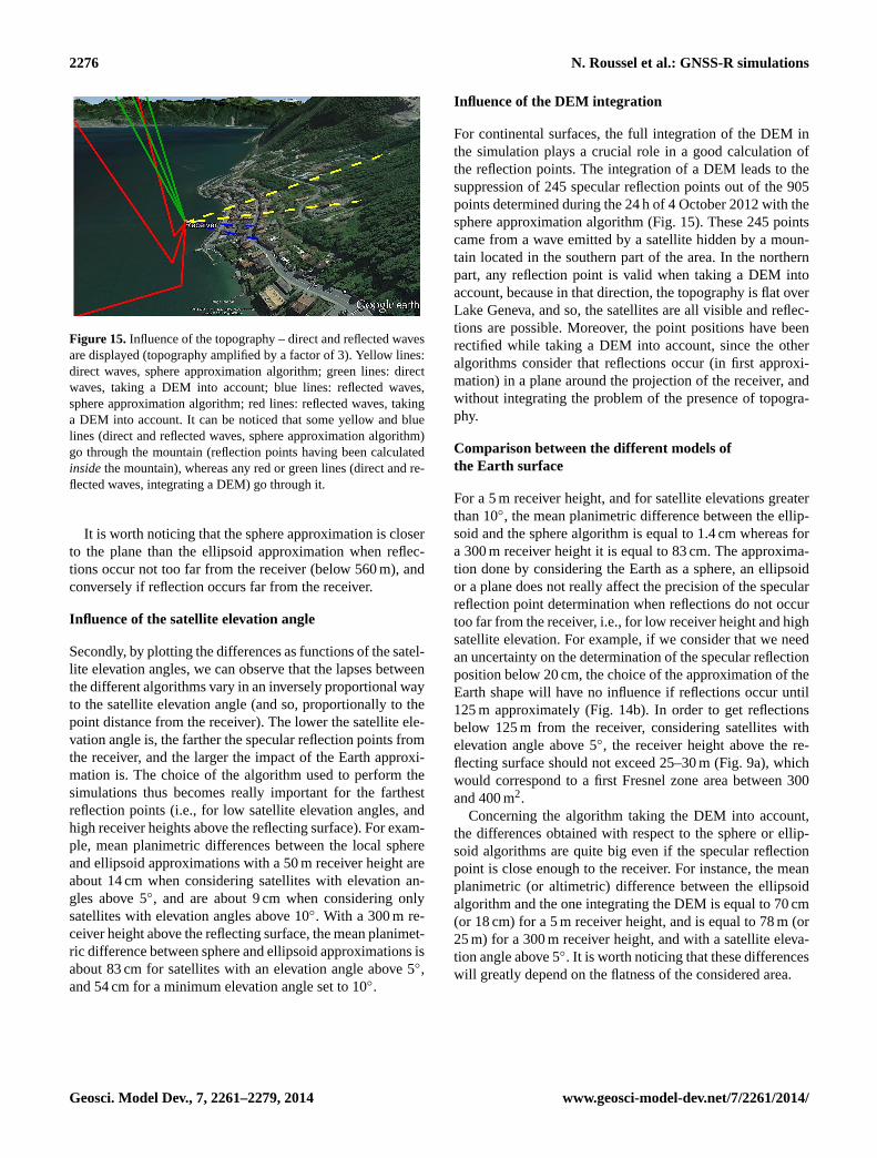
Figure 15. Influence of the topography – direct and reflected wavesare displayed (topography amplified by a factor of 3). Yellow lines:direct waves, sphere approximation algorithm; green lines: directwaves, taking a DEM into account; blue lines: reflected waves,sphere approximation algorithm; red lines: reflected waves, takinga DEM into account. It can be noticed that some yellow and bluelines (direct and reflected waves, sphere approximation algorithm)go through the mountain (reflection points having been calculatedinsidethe mountain), whereas any red or green lines (direct and re-flected waves, integrating a DEM) go through it.

It is worth noticing that the sphere approximation is closerto the plane than the ellipsoid approximation when reflec-tions occur not too far from the receiver (below 560 m), andconversely if reflection occurs far from the receiver.

Influence of the satellite elevation angle

Secondly, by plotting the differences as functions of the satel-lite elevation angles, we can observe that the lapses betweenthe different algorithms vary in an inversely proportional wayto the satellite elevation angle (and so, proportionally to thepoint distance from the receiver). The lower the satellite ele-vation angle is, the farther the specular reflection points fromthe receiver, and the larger the impact of the Earth approxi-mation is. The choice of the algorithm used to perform thesimulations thus becomes really important for the farthestreflection points (i.e., for low satellite elevation angles, andhigh receiver heights above the reflecting surface). For exam-ple, mean planimetric differences between the local sphereand ellipsoid approximations with a 50 m receiver height areabout 14 cm when considering satellites with elevation an-gles above 5◦, and are about 9 cm when considering onlysatellites with elevation angles above 10◦. With a 300 m re-ceiver height above the reflecting surface, the mean planimet-ric difference between sphere and ellipsoid approximations isabout 83 cm for satellites with an elevation angle above 5◦,and 54 cm for a minimum elevation angle set to 10◦.

Influence of the DEM integration

For continental surfaces, the full integration of the DEM inthe simulation plays a crucial role in a good calculation ofthe reflection points. The integration of a DEM leads to thesuppression of 245 specular reflection points out of the 905points determined during the 24 h of 4 October 2012 with thesphere approximation algorithm (Fig.15). These 245 pointscame from a wave emitted by a satellite hidden by a moun-tain located in the southern part of the area. In the northernpart, any reflection point is valid when taking a DEM intoaccount, because in that direction, the topography is flat overLake Geneva, and so, the satellites are all visible and reflec-tions are possible. Moreover, the point positions have beenrectified while taking a DEM into account, since the otheralgorithms consider that reflections occur (in first approxi-mation) in a plane around the projection of the receiver, andwithout integrating the problem of the presence of topogra-phy.

Comparison between the different models ofthe Earth surface

For a 5 m receiver height, and for satellite elevations greaterthan 10◦, the mean planimetric difference between the ellip-soid and the sphere algorithm is equal to 1.4 cm whereas fora 300 m receiver height it is equal to 83 cm. The approxima-tion done by considering the Earth as a sphere, an ellipsoidor a plane does not really affect the precision of the specularreflection point determination when reflections do not occurtoo far from the receiver, i.e., for low receiver height and highsatellite elevation. For example, if we consider that we needan uncertainty on the determination of the specular reflectionposition below 20 cm, the choice of the approximation of theEarth shape will have no influence if reflections occur until125 m approximately (Fig.14b). In order to get reflectionsbelow 125 m from the receiver, considering satellites withelevation angle above 5◦, the receiver height above the re-flecting surface should not exceed 25–30 m (Fig.9a), whichwould correspond to a first Fresnel zone area between 300and 400 m2.

Concerning the algorithm taking the DEM into account,the differences obtained with respect to the sphere or ellip-soid algorithms are quite big even if the specular reflectionpoint is close enough to the receiver. For instance, the meanplanimetric (or altimetric) difference between the ellipsoidalgorithm and the one integrating the DEM is equal to 70 cm(or 18 cm) for a 5 m receiver height, and is equal to 78 m (or25 m) for a 300 m receiver height, and with a satellite eleva-tion angle above 5◦. It is worth noticing that these differenceswill greatly depend on the flatness of the considered area.

Geosci. Model Dev., 7, 2261–2279, 2014 www.geosci-model-dev.net/7/2261/2014/

N. Roussel et al.: GNSS-R simulations 2277

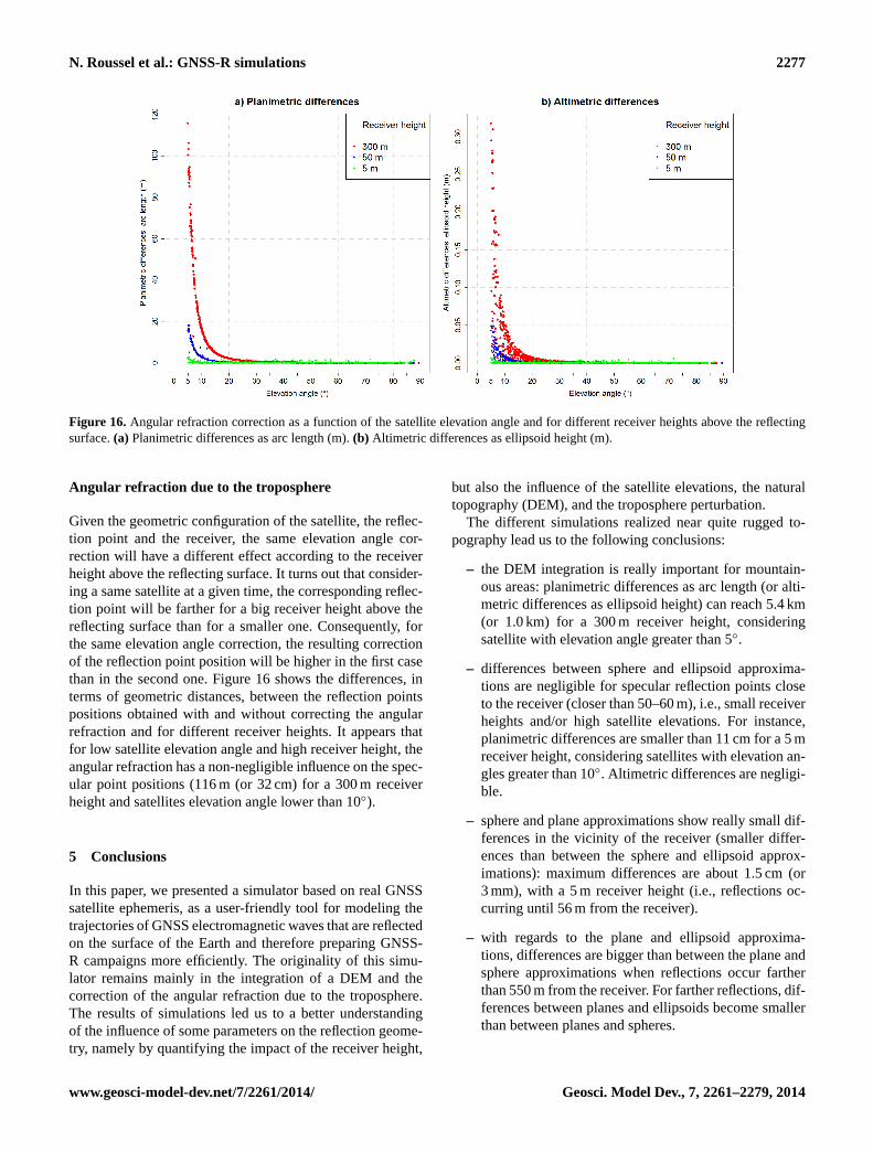
Figure 16. Angular refraction correction as a function of the satellite elevation angle and for different receiver heights above the reflectingsurface.(a) Planimetric differences as arc length (m).(b) Altimetric differences as ellipsoid height (m).

Angular refraction due to the troposphere

Given the geometric configuration of the satellite, the reflec-tion point and the receiver, the same elevation angle cor-rection will have a different effect according to the receiverheight above the reflecting surface. It turns out that consider-ing a same satellite at a given time, the corresponding reflec-tion point will be farther for a big receiver height above thereflecting surface than for a smaller one. Consequently, forthe same elevation angle correction, the resulting correctionof the reflection point position will be higher in the first casethan in the second one. Figure16 shows the differences, interms of geometric distances, between the reflection pointspositions obtained with and without correcting the angularrefraction and for different receiver heights. It appears thatfor low satellite elevation angle and high receiver height, theangular refraction has a non-negligible influence on the spec-ular point positions (116 m (or 32 cm) for a 300 m receiverheight and satellites elevation angle lower than 10◦).

5 Conclusions

In this paper, we presented a simulator based on real GNSSsatellite ephemeris, as a user-friendly tool for modeling thetrajectories of GNSS electromagnetic waves that are reflectedon the surface of the Earth and therefore preparing GNSS-R campaigns more efficiently. The originality of this simu-lator remains mainly in the integration of a DEM and thecorrection of the angular refraction due to the troposphere.The results of simulations led us to a better understandingof the influence of some parameters on the reflection geome-try, namely by quantifying the impact of the receiver height,

but also the influence of the satellite elevations, the naturaltopography (DEM), and the troposphere perturbation.

The different simulations realized near quite rugged to-pography lead us to the following conclusions:

– the DEM integration is really important for mountain-ous areas: planimetric differences as arc length (or alti-metric differences as ellipsoid height) can reach 5.4 km(or 1.0 km) for a 300 m receiver height, consideringsatellite with elevation angle greater than 5◦.

– differences between sphere and ellipsoid approxima-tions are negligible for specular reflection points closeto the receiver (closer than 50–60 m), i.e., small receiverheights and/or high satellite elevations. For instance,planimetric differences are smaller than 11 cm for a 5 mreceiver height, considering satellites with elevation an-gles greater than 10◦. Altimetric differences are negligi-ble.

– sphere and plane approximations show really small dif-ferences in the vicinity of the receiver (smaller differ-ences than between the sphere and ellipsoid approx-imations): maximum differences are about 1.5 cm (or3 mm), with a 5 m receiver height (i.e., reflections oc-curring until 56 m from the receiver).

– with regards to the plane and ellipsoid approxima-tions, differences are bigger than between the plane andsphere approximations when reflections occur fartherthan 550 m from the receiver. For farther reflections, dif-ferences between planes and ellipsoids become smallerthan between planes and spheres.

www.geosci-model-dev.net/7/2261/2014/ Geosci. Model Dev., 7, 2261–2279, 2014

2278 N. Roussel et al.: GNSS-R simulations

– the angular refraction due to troposphere can be negligi-ble with regards to the position of the specular reflectionpoint when the receiver height is below 5 m, but is ab-solutely mandatory otherwise, particularly for satelliteswith low elevation angles where the correction to applyis exponential.

As a final remark, it is worth reminding the reader that thefarther the specular reflection point is from the receiver, themore important the influence of the different error sourceswill be: Earth approximation, DEM integration, angular re-fraction. The farthest specular reflection points will be ob-tained for high receiver height and low satellite elevation.This simulator is likely to be of great help for the prepara-tion of in situ experiments involving the GNSS-R technique.Further developments of the simulator will be implementedsoon, such as a receiver installed on a moving platform inorder to map the area covered by airborne GNSS-R measure-ment campaigns and on-board a LEO satellite.

Acknowledgements.This work was funded by CNES in theframework of the TOSCA project “Hydrologie, Océanogra-phie par Réflectométrie GNSS (HORG)” and by the RTRASTAE foundation in the framework of the “Potentialités dela Réflectométrie GNSS In Situ et Mobile (PRISM)” project.Nicolas Roussel is supported by a PhD granted from the FrenchMinistère de l’Enseignement Supérieur et de la Recherche (MESR).

Edited by: R. Marsh

References

Beckmann, P. and Spizzichino, A.: Scattering of ElectromagneticWaves from Rough Surfaces, Artech House Publishers, ISBN 0-89006-238-2, 1987.

Billich, A. L.: Improving the Precision and Accuracy of GeodeticGPS: Applications to Multipath and Seismology, PhD. B.S., Uni-versity of Texas at Austin, M.S., University of Colorado, 2004.

Boehm, J., Niell, A., Tregoning, P., and Schuh, H.: Global MappingFunction (GMF): A new empirical mapping function based onnumerical weather model data, Geophys. Res. Lett., 33, L07304,doi:10.1029/2005GL025546, 2006a.

Boehm, J., Werl, B., and Schuh, H.: Troposphere mapping func-tions for GPS and very long baseline interferometry from Eu-ropean Centre for Medium-Range Weather Forecasts opera-tional analysis data, J. Geophys. Res. Sol.-Earth, 111, B02406,doi:10.1029/2005JB003629, 2006.

Cardellach, E., Fabra, F., Rius, A., Pettinato, S., and Daddio, S.:Characterization of Dry-snow Sub-structure using GNSS Re-flected Signals, Remote Sens. Environ., 124, 122–134, 2012.

Chen, G. and Herring, T.: Effects of atmospheric azimuthal asym-metry on the analysis of space geodetic data, J. Geophys. Res.Sol.-Earth, 102, 20489–20502, doi:10.1029/97JB01739, 1997.

Géegout, P., Biancale, R., and Soudarin, L.: Adaptive MappingFunctions to the azimuthal anisotropy of the neutral atmosphere,J. Geodesy., 85, 661–667, 2011.

Gleason, S.: Remote Sensing of Ocean, Ice and Land Surfaces Us-ing Bistatically Scattered GNSS Signals From Low Earth Orbit,Thesis (Ph.D.), University of Surrey, 2006.

Gleason, S., Lowe, S., and Zavorotny, V.: Remote sensing us-ing bistatic GNSS reflections, GNSS Applications and methods,399–436, 2009.

Helm, A.: Ground based GPS altimetry with the L1 openGPSreceiver using carrier phase-delay observations of reflectedGPS signals, Thesis (Ph.D.), Deutsches GeoForschungsZentrum(GFZ), 164 pp., 2008.

Hobiger, T., Ichikawa, R., Takasu, T., Koyama, Y., and Kondo, T.:Ray-traced troposphere slant delays for precise point positioning,Earth Planet. Space, 60, e1–e4, 2008.

Jarvis, J., Reuter, H., Nelson, A., and Guevara, E.: Hole-filledSRTM for the globe, CGIAR-CSI SRTM 90 m DAtabase, Ver-sion 4, CGIAR Consort for Spatial Inf., 2008.

Katzberg, S., Torres, O., Grant, M. S., and Masters, D.: Utilizingcalibrated GPS reflected signals to estimate soil reflectivity anddielectric constant: results from SMEX02, Remote Sens. Envi-ron., 100, 17–28, 2006.

Komjathy, A., Zavorotny, V., Axelrad, P., Born, G., and Garrison,J.: GPS signal scattering from sea surface, Wind speed retrievalusing experimental data and theoretical model, Remote Sens. En-viron., 73, 162–174, 2000.

Kostelecky, J., Klokocnik, J., and Wagner, C. A.: Geometry andaccuracy of reflecting points in bistatic satellite altimetry, J.Geodesy, 79, 421–430, doi:10.1007/s00190-005-0485-7, 2005.

Lagler, K., Schindelegger, M., Boehm, J., Krsn, H., and Nils-son, T.: GPT2: Empirical slant delay model for radio spacegeodetic techniques, Geophys. Res. Lett., 40, 1069–1073,doi:10.1002/grl.50288, 2013.

Larson, K. M. and Nievinski, F. G.: GPS snow sensing: results fromthe EarthScope Plate Boundary Observatory, GPS Solut., 17, 41–52, doi:10.1007/s10291-012-0259-7, 2013.

Löfgren, J. S., Rüdiger, H., and Scherneck, H. G.: Sea-Level analy-sis using 100 days of reflected GNSS signals, Proceedings of the3rd International Colloquium – Scientific and Fundamental As-pects of the Galileo Programme, 31 August–2 September 2011,Copenhagen, Denmark, (WPP 326) 5 pp., 2011.

Lowe, S. T., Zuffada, C., Chao, Y., Kroger, P., Young, L. E.,and LaBrecque, J. L.: 5-cm-Precision aircraft ocean altime-try using GPS reflections, Geophys. Res. Lett., 29, 1375,doi:10.1029/2002GL014759, 2002.

Marini, J. W.: Correction of satellite tracking data for anarbitrary tropospheric profile, Radio Sci., 7, 223–231.doi:10.1029/RS007i002p00223, 1972.

Martin-Neira, M.: A passive reflectometry and interferometry sys-tem (PARIS): Application to ocean altimetry, ESA J-Eur. SpaceAgen., 17, 331–355, 1993.

Nafisi, V., Urquhart, L., Santos, M. C., Nievinski, F. G., Bohm,J., Wijaya, D. D., Schuh, H., Ardalan, A. A., Hobiger, T.,Ichikawa, R., Zus, F., Wickert, J., and Gegout, P.: Comparison ofRay-Tracing Packages for Troposphere Delays, Geosci. RemoteSens., 50, 469–481, doi:10.1109/TGRS.2011.2160952, 2012.

NASA and NIMA: The Development of the Joint NASA GSFC andthe National Imagery and Mapping Agency (NIMA) Geopoten-tial Model EGM96, NASA/TP-1998-206861, 1998.

Niell, A.: Preliminary evaluation of atmospheric mapping functionsbased on numerical weather models, Proceedings of the First

Geosci. Model Dev., 7, 2261–2279, 2014 www.geosci-model-dev.net/7/2261/2014/

N. Roussel et al.: GNSS-R simulations 2279

COST Action 716 Workshop Towards Operational GPS Mete-orology and the Second Network Workshop of the InternationalGPS Service (IGS), 26, 475–480, 2001.

Nievinski, F. G. and Santos, M. C.: Ray-tracing options to mitigatethe neutral atmosphere delay in GPS, Geomatica, 64, 191–207,2010.

NIMA: National Imagery and Mapping Agency: Departementof Defense Wolrd Geodetic System 1984. NIMA Stock No.DMATR83502WGS84, NSN 7643-01-402-0347, 1997.

Nocedal, J. and Wright, S. J.: Numerical Optimization, Springer,ISBN 978-0-387-30303-1, USA (TB/HAM), 2006.

Rius, A., Aparicio, J. M., Cardellach, E., Martin-Neira, M.,and Chapron, B.: Sea surface state measured using GPSreflected signals, Geophys. Res. Lett., 29, 37-1–37-4,doi:10.1029/2002GL015524, 2002.

Rius, A., Noque’s-Correig, O., Ribo, S., Cardellach, E., Oliveras,S., Valencia, E., Park, H., Tarongi, J. M., Camps, A., Van DerMarel, H., Van Bree, R., Altena, B., and Martin-Neira, M.: Al-timetry with GNSS-R interferometry: first proof of concept Ex-periment, GPS Solutions, 16, 231–241, doi:10.1007/s10291-011-0225-9, 2012.

Rodriguez, E., Morris, C. S., Belz, J. E., Chapin, E. C., Mar-tin, J. M., Daffer, W., and Hensley, S.: An assessment ofthe SRTM topographic products, Technical Report D-31639,JPL/NASA,2005.

Rodriguez-Alvarez, N., Bosch-Lluis, X., Camps, A., Vall-Llossera,M., Valencia, E., Marchan-Hernandez, J. F., and Ramos-Perez, I.:Soil moisture retrieval using GNSS-R techniques: Experimentalresults over a bare soil field, IEEE Trans. Geosci. Remote Sens.,47, 3616–3624, 2009.

Rodriguez-Alvarez, N., Camps, A., Vall-Llossera, M., Bosch-Lluis, X., Monerris, A., Ramos-Perez, I. Valencia, E., Marchan-Hernandez, J. F., Martinez-Fernandez, J., Baroncini-Turricchia,G., Pérez-Gutiérrez, C., and Sanchez, N.: Land Geophysical Pa-rameters Retrieval Using the Interference Pattern GNSS-R Tech-nique, IEEE Trans. Geosci. Remote Sens., 49, 71–84, 2011.

Ruffini, G., Soulat, F., Caparrini, M., Germain, O., and Martin-Neira, M.: The Eddy Experiment: Accurate GNSS-R oceanaltimetry from low altitude aircraft, Geophys. Res. Lett., 31,L12306, doi:10.1029/2004GL019994, 2004.

Semmling, A. M., Beyerle, G., Stosius, R., Dick, G., Wickert, J.,Fabra, F., Cardellach, E., Ribo, S., Rius, A., Helm, A., Yudanov,S. B., and d’Addio, S.: Detection of Arctic Ocean tides using in-terferometric GNSS-R signals, Geophys. Res. Lett., 38, L04103,doi:10.1029/2010GL046005, 2011.

Soulat, F., Caparrini, M., Germain, O., Lopez-Dekker, P., Taani,M., and Ruffini, G.: Sea state monitoring using coastal GNSS-R,Geophys. Res. Lett., 31, L21303, doi:10.1029/2004GL020680,2004.

Treuhaft, P., Lowe, S., Zuffada, C., and Chao, Y.: 2-cm GPS altime-try over Crater Lake, Geophys. Res. Lett., 28, 4343–4436, 2004.

Wagner, C. and Klokocnik, C.: The value of ocean reflections ofGPS signals to enhance satellite altimetry: data distribution anderror analysis, J. Geodesy, 77, 128–138, doi:10.1007/s00190-002-0307-0, 2003.

Zavorotny, A. U. and Voronovich, A. G.: Scattering of GPS sig-nals from the ocean with wind remote sensing application, IEEETrans. Geosci. Remote Sens., 38, 951–964, 2000.

Zus, F., Bender, M., Deng, Z., Dick, G., Heise, S., Shang-Guan,M., and Wickert, J.: A methodology to compute GPS slant totaldelays in a numerical weather model, Radio Sci., 47, RS2018,doi:10.1029/2011RS004853, 2012.

www.geosci-model-dev.net/7/2261/2014/ Geosci. Model Dev., 7, 2261–2279, 2014