Simulation of the Robot Roller Hemming process · 2011-08-28 · Finite element analysis of the...
104
Transcript of Simulation of the Robot Roller Hemming process · 2011-08-28 · Finite element analysis of the...

Simulation of the Robot Roller Hemming process
Simulation of the Robot Roller Hemming process
Jonkers, B.
Bunschoten, November 2006
Voestalpine Polynorm Automotive, Bunschoten
Universiteit Twente
Department of Mechanical Engineering Applied Mechanics
Voestalpine Polynorm Automotive Laurens van der Sande Mathieu Brand Universiteit Twente Prof.dr.ir. J. Huétink Dr.ir. Timo Meinders Dr. Ton Bor Ir. Maarten van Riel

Simulation of the Robot Roller Hemming process
Acknowledgements The work presented in this master thesis was carried out at the department Corporate Engineering of Voestalpine Polynorm Bunschoten, from February 2006 to December 2006. I would like to thank several people for their cooperation and support in this project. First of all, my supervisors, Laurens van der Sande and Mathieu Brand at Voestalpine Polynorm and Timo Meinders at the department of Applied Mechanics, University of Twente. They all guided me very well through the project and had a significant influence in the reviewing of this work. Furthermore, Laurens guided me in the beginning and made me familiar within the company while Mathieu assisted me in the modeling process. They were always willing to help me with all sorts of problems. I also would like to thank Hans Francken for his contribution. His experience in forming simulations was helpful during progress discussions with Laurens, Mathieu and me. In these discussions more insight in the robot roller hemming process was gained. Furthermore I would like to thank all my colleagues at Corporate Engineering for their help and encouragement. They provided for a pleasant working environment. Finally, I would like to thank family and friends who always showed an interest in my work and were always willing to help me.

Simulation of the Robot Roller Hemming process
Summary At Voestalpine Polynorm, hemming is used as an assembly method for closures (i.e. doors, hoods, tailgates and trunklids) in automotive bodies. Hemming is a process by which a metal sheet edge of an outer part is bent around an inner part. Robot roller hemming is a relatively new process. The process will be applied more and more in the future due to market demands and process development. Too little fundamental process knowhow is available. Achieving and maintaining the right product quality is therefore a trial-and-error process. Finite element analysis of the robot roller hemming process helps reducing this try-out phase. Goals are to create a more stable process and achieving the right product quality. The main targets are to create process setting guidelines which control the dimensional and surface quality and reduce the overall process time. The simulations are performed with the finite element package Abaqus®. The development of a 3D robot roller hemming simulation model is described in this report. The work presented in this report concentrates mainly on predicting the reduction in size of the outer part, called roll-in. The dimensions of the outer part have to be compensated for this roll-in, to obtain a finished product with the right dimensions. Started is with a simple 2D simulation model which can simulate the die and tabletop hemming process. The use of implicit and explicit solution methods is investigated. Both solution methods can be applied in (quasi-static) hemming simulations. An element-type comparison is performed with a small 3D tabletop model. In this implicit simulation model both solid and shell elements are used in the simulations. This way an accurate and economical element is chosen for the 3D robot roller hemming model. The continuum shell element is the most suitable element-type for large 3D robot roller hemming models. This element-type showed a realistic roll-in behaviour (roll-in after prehemming and this amount of roll-in was reduced during final hemming) during the simulation, with the smallest amount of simulation time. The differences between shell and solid elements were smaller after prehemming than after final hemming. A parameter study of the prehemming step is performed on straight flat-surface parts based on a ‘Design of Experiments’. Parameters which have a big influence on the roll-in of the process are identified with this set of simulations. After this, a response surface model is created, from the roll-in response of the simulation model on the two most important process parameters. This can be used by process engineers and robot programmers to create a stable process window by choosing the optimal process setting ranges. Furthermore, guidelines are given to prevent the forming of wave patterns along the flange which disturb the quality of finished products.

Simulation of the Robot Roller Hemming process
Contents Acknowledgements iii Summary v 1. Introduction 6 2. Background information Hemming 9
2.1. Description of a hem 9 2.2. Hemming Technologies 10
2.2.1. Die Hemming 11 2.2.2. Tabletop Hemming 11 2.2.3. Robot Roller Hemming 13
2.3. Hemming Quality 14 2.3.1. Dimensional Quality 14 2.3.2. Surface Quality 15
2.4. Problem Description 16
3. Basic principles of the FEA method 18
3.1. The finite element method 18 3.2. Solving a structure with the finite element method 19
3.2.1. Implicit solution method 22 3.2.2. Explicit solution method 23
4. Simulation of the hemming process 24
4.1. Literature study of hemming simulations 24 4.2. Approach of the hemming simulations 25
5. Die and Tabletop hemming simulations 27
5.1. 2D simulation model development 27 5.1.1. Validation information from practice 27 5.1.2. 2D simulation model 29 5.1.3. Results 38
5.2. Influence of element-types on the results of a tabletop simulation 42 5.2.1. Solid element 43 5.2.2. Shell element 43 5.2.3. Results 45
5.3. Conclusions 46
6. Robot Roller hemming simulations 47
6.1. Situation in practice 47 6.1.1. Set up of the robot roller hemming process 47 6.1.2. Specific robot roller hemming parameters 48
6.2. Robot roller hemming simulation model development 50 6.2.1. Starting point of the simulations 51 6.2.2. Complete process – implicit simulations 53 6.2.3. Explicit simulations 57 6.2.4. Conclusions 58
7. Parameter study based on a ‘Design of Experiments’ 59
7.1. Design of experiments 59 7.1.1. Full or fractional factorial designs 60
7.2. Parameters investigated 63 7.3. Results 66

Simulation of the Robot Roller Hemming process
7.4. Process optimization 69 7.4.1. Optimize on roll-in values 69 7.4.2. Wave pattern reduction 72 7.4.3. Conclusions 81
8. Conclusions and Recommendations 82
8.1. Conclusions 82 8.2. Recommendations 83
List of References 85 Appendix A: Assignment 81 Appendix B: Implicit method 83 Appendix C: Explicit method 85 Appendix D: Contact interactions of both solution methods 91 Appendix E: Simulation model and results in detail 92

Simulation of the Robot Roller Hemming process
1. Introduction Voestalpine Polynorm is a supplier to the automotive industry, specialized in project management, product development, engineering and production of body panels and components made from steel, aluminum, plastic and hybrid materials. As a result of constantly increasing product quality requirements demanded by the automotive industry and the competition among suppliers, process optimization is desired. This helps to increase product quality and to reduce the costs. For the assembly production of closures (opening parts like doors and hoods) two parts are assembled together, an outer part is assembled with an inner part. All the parts of a hood are depicted in Figure 1-1. One of Polynorm’s objectives is to expand its assembly capacities and capabilities. One assembly method is called hemming.
Figure 1-1
Parts of a hood closure [Ultralight steel Auto Closures – Ulsac, may 2000] Hemming is a process which consists in joining two sheet metal parts by plastic deformation. A metal sheet edge of an outer part is bent around an inner part by hemming to create a hem. This process is depicted in Figure 1-2. To hem closures, several technologies are available on the market, such as die hemming and tabletop hemming.
Figure 1-2
A hem. The outer part (orange) edge is bent around an inner part (black) Robot roller hemming was introduced at the market in the late nineties and has been applied by Polynorm since the year 2000. A roller is guided along a product by a robot which bends the outer part around the inner part. Compared to die and tabletop hemming, the product specific production equipment required for the assembly production is reduced to a minimum. This makes the process suitable for the production of many different parts, as it can simply be re-programmed for other products. The process steps of a robot roller hemming process are depicted in Figure 1-3 below (right three figures) together with an overview of the installation (left). The edge of the outer part (grey) is bent in three steps, two prehemming steps (middle two figures) and one final hemming step (depicted right). In between the hemming steps the orientation of the roller is varied.
Striker Assy.
Hood Outer
Reinf. Hinge
Hood Inner
Reinf. Striker

Simulation of the Robot Roller Hemming process
Figure 1-3
Robot roller hemming installation (left) with three hemming steps (right three) schematically drawn Currently too little fundamental know-how is available with regard to the robot roller hemming process itself. Achieving and maintaining the required product quality is therefore a ‘trial-and-error’ process. To enable a more stable process and achieve better product quality as well as a shorter time-to-market, finite element analyses (FEA) simulations of the robot roller hemming process would be helpful to understand, define and optimize the process. The main targets of this assignment are to obtain process setting guidelines which control the dimensional and surface quality and to reduce the overall process time. These targets can be achieved by building a three dimensional FEA simulation model which can describe the robot roller hemming process. The work presented in this report concentrates mainly on predicting the reduction in size of the outer part, called roll-in. This is depicted in Figure 1-4 below on the left. During the hemming process the outer edge of the outer panel rolls in, reducing the dimensions of the finished product. The dimensions of the outer part have to be compensated for this roll-in, to obtain a finished product with the right dimensions.
Figure 1-4
Roll-in of an outer panel (left); The forming of wave patterns which decreases the quality (right) Another part of this work concentrated on the reduction of wave patterns along the flange during the hemming process. These defects are depicted right in Figure 1-4. This is a specific robot roller hemming defect. During the prehemming step(s) a wave pattern is formed in the flange (depicted above right). After the final hemming step these waves are not always fully flattened out, deteriorating the products quality (depicted below right). The structure of this report is as follows. The backgrounds of hemming are given in chapter 2. The main process types, die, tabletop and robot roller hemming are each described individually. Product quality specific for hemming areas is divided into dimensional and surface quality. Basic FEA information is given in chapter 3. Two basic solution methods (implicit and explicit) are described here which both can be applied in hemming simulations. Chapter 4 contains a literature study of previous performed

Simulation of the Robot Roller Hemming process
hemming simulations together with the approach of this report. A 2D simulation model is developed in chapter 5 which can simulate the die and tabletop processes. Information from previous studies is used to validate this model. Both the implicit and explicit solution methods are applied. A small 3D tabletop model is simulated with both solid and shell elements to find a suitable element for the 3D robot roller hemming simulation model. The development of this simulation model is given in chapter 6. The main parameters of the process are also given here. In chapter 7 a parameter study is performed based on a ‘Design of Experiments’. This parameter study indicates parameters with a big influence on roll-in, which there after are used to create a roll-in response surface of the model. Different quality optimization methods are also described in this chapter. These methods are based on a roll-in optimization and a decrease in the forming of wave patterns along the flange during the hemming steps. Finally the conclusions and recommendations of this report are given in chapter 8.

Simulation of the Robot Roller Hemming process
2. Background information Hemming In this chapter the basic information about hemming needed to understand this report is given. The available production methods, including their main parameters are explained in section 2.1. In section 2.2 the hemming quality aspects are described divided into dimensional and surface quality. Finally the reason for simulating the robot roller hemming process is illustrated in section 2.3.
Figure 2-1
The hemming process; outer part (orange) hemmed around an inner part (black)
2.1. Description of a hem A hem is a bent edge of a metal sheet. Hemming is a process by which that edge is bent. In Figure 2-1 an outer part (orange) is bent around an inner part (black) by hemming. It gives a neat and a compact joint. However, it is less strong than a welded joint. It is on the other hand possible to combine hemming with other additional joining methods, for instance gluing, in order to increase the strength of the joint. Hemming (Figure 2-1) is mainly used as an assembly method for closures in automotive bodies. Closures are the closing parts of a car (i.e. doors, hoods, tailgates and trunklids). The parts for a hood assembly are depicted in Figure 2-2. Increased safety and esthetics are other functions of a hem. The ongoing development of hemming technologies leads to new product development opportunities and new applications.
Figure 2-2
Exploded view of a hood; the inner part with reinforcements is assembled with the outer part by hemming The manufacturing process of a closure starts in press lines where the components are stamped. The outer part is manufactured by deep drawing (depicted left in Figure 2-3 where the outer part is colored red), followed by trimming (depicted right in Figure 2-3).
Striker Assy.
Hood Outer
Reinf. Hinge
Hood Inner
Reinf. Striker

Simulation of the Robot Roller Hemming process
Figure 2-3 Part of the manufacturing process of a closure; Left: deep drawing of the outer part (red), Right: trimming the outer part
After the trimming process the edges of the outer part (which are to be hemmed) are bent. This process is called flanging (depicted in Figure 2-4). Flanging consists in the bending of the sheet edge with an angle approximately equal to 90°. The yellow tools in Figure 2-4 bent the edge of the outer part. The opening angle of the bent edge is depicted right in Figure 2-4.
Figure 2-4 The flanging process; Outer part flanged in a flanging die (left), flanging process schematically (right)
In the bonding process adhesives are to give additional strength, corrosion protection and dampening to the future closure. The outer and inner part are combined together in the marriage process. The product is finally assembled by the hemming process (with optional additional spot welds). The next section describes the commonly used hemming technologies.
2.2. Hemming Technologies Different hemming technologies are available. They can be distinguished by several factors, for instance investment level, process time and technical concept. The technical differences between them are described here. Three main process types are available: die, tabletop and robot roller hemming. Despite their differences they all have the similarity that they divide the hemming in different steps: one or more prehemming steps (left two pictures of Figure 2-5) and one final hemming step (depicted right in Figure 2-5) to complete the hemming.
Figure 2-5
The hemming steps; prehemming (left two pictures) and final hemming (right)

Simulation of the Robot Roller Hemming process
This is done to assure that the hem meets the requirements. The amount of prehemming steps is dependent on the opening angle of the flange and the type of process. The main process types are explained below. Special hemming installations do exist outside these three main groups but are not considered in this report.
2.2.1. Die Hemming The hemming with the help of presses is called die hemming. It is probably the oldest way of automated hemming. In Figure 2-6 an example of a die hem installation is given. The installation itself is universal. Only the parts in the purple dotted box in Figure 2-6 are product specific. These parts include the hemming die. All the other components are universal.
Figure 2-6
A die hemming press (Hyrotec) For flange opening angles of 90° the process is performed in two hemming steps: one prehemming and one final hemming step. Two presses are needed for a conventional die hemming process where each press performs a hemming step (one prehemming and one final hemming step). The movement pattern of this process is vertical. Both the pre- and final hemming steps are performed vertical (Figure 2-7).
Figure 2-7
Movement patterns of both hemming steps based on die hemming; prehemming (left) and final hemming (right) The hemming is performed fast. The die hemming installations are therefore very suited for high volume production. New products can be hemmed with the same installation when the hemming die (blue parts in Figure 2-6) is replaced.
2.2.2. Tabletop Hemming More sophisticated hemming installations are the tabletop systems. An example of a complete tabletop system is depicted in Figure 2-8. The prehemming tools hem the product from the side (horizontally). The final hemming is performed vertical. A tabletop hemming installation is completely product specific.

Simulation of the Robot Roller Hemming process
Figure 2-8
A tabletop hemming installation There are a lot of different tabletop systems available with their own specific features. The movement pattern of the prehemming step can be horizontal, vertical or a combination of both. In Figure 2-9 two tabletop hemming systems are depicted with a vertical (left) and a horizontal (right) movement pattern for the prehemming step. The outer part is colored red. The lower step in the figures is the prehemming step. Final hemming is the upper step.
Figure 2-9
Movement patterns of of the prehemming step of different tabletop systems: vertical movement pattern (left) and horizontal movement pattern (right). Product is lifted between the steps (lower step is prehemming)
The product assembled with a tabletop installation is generally hemmed in two steps (similar to die systems). Both the steps are integrated in one installation. More complex product geometries can be hemmed with tabletop systems. The movement patterns of the tabletop variant used in this report are given in Figure 2-10.
Figure 2-10
Movement patterns of both hemming steps based on the tabletop hemming variant covered in this report; prehemming (left) and final hemming (right)
The tabletop hemming process is suited for high volume production. Cycle times are similar to die hemming. It is easy to integrate a tabletop installation on an assembly line. A disadvantage of the installation is the high investment level. The system is very expensive because the whole installation is product specific.

Simulation of the Robot Roller Hemming process
2.2.3. Robot Roller Hemming The robot roller hemming process is unique to other hemming processes by its completely different movement pattern (depicted left in Figure 2-12). A robot guides a roller parallel along the flange. Complete products can be hemmed with the same roller (in Figure 2-11 on the left a flexible robot cell is shown were three different products are hemmed). Also more robots can be applied in the hemming of a product to speed up the hemming process. In Figure 2-11 on the right different sides of a product are hemmed with two different robots.
Figure 2-11
Left: Robot cell were three different product (hood and both doors) are hemmed with the same robot (ABB) Right: Two robots hem different sides of a product
The roll hemming process is generally carried out in three steps. In between the hemming steps the orientation (angle) of the roller is changed (depicted right in Figure 2-12).
Figure 2-12
Robot roller hemming process. Left: movement pattern parallel along the flange. Right: the standard three step roll forming process;
Current robot roller hemming forming speeds of 500 mm/s are used on straight segments. Different geometries of rollers have an effect on the hemming process. Diameters of the roller can be varied. The main advantages of this process are its low investment level for each new product, the lead time to design and manufacture product specific robot roller hemming equipment. The method is slower than tabletop or die systems, which currently restricts the robot roller hemming application to low and middle volume production. New development in robot roller hemming focuses on reduction of cycle times, which will make the process more suitable for higher production volumes as well. Two step roller hemming and higher forming speeds are in development nowadays. The different process types have different effects on the quality and dimensions of the complete hemmed product. The next section describes at which appearances (dimensional and surface) the quality of a hem is checked.

Simulation of the Robot Roller Hemming process
2.3. Hemming Quality Hemming is used mainly for the assembly of closures in automotive bodies. The outer appearance of the vehicle is therefore influenced by the outcome of the hemming process. It is therefore important to be able to predict the final shape and surface quality of the finished product and to determine the parameters which influence it. The quality areas involved in the hemming are given below. The quality areas can be divided in dimensional and surface quality.
2.3.1. Dimensional Quality The dimensional quality is mainly given by two terms, the gap and the flush of a panel/part. The gap and the flush are the most important terms related to hemming.
Gap Closures create gaps on the outer skin of the car due to the fact that they have to be able to open/close properly. In Figure 2-13 three examples of panel gaps are given.
Figure 2-13
Hood/Front fender gap (left); Front/Rear door gap (middle); Rear door/Rear fender gap (right) A general trend in the automotive industry today is to try to reduce the gaps between the body parts, therefore it is very important to be able to control/predict the roll-in of the hem (see Figure 2-14) and to compensate for it. The roll-in of the hem is defined as the distance between the outer radius of the hem and the original flange of the panel.
Figure 2-14
The roll-in of a hem In corners and on curvatures the roll-in can be different than on straight flat areas. Even roll-out (increased panel size) is possible in sharp corners. The roll-in is thus not the same along a product. On the rear door depicted right in Figure 2-13 opposite geometries (convex/concave shaped) with different effects on the roll-in come together. They must create an evenly distributed gap (gap shown by blue arrows must equal gap shown with red arrows). It is therefore important to control the mechanism behind the

Simulation of the Robot Roller Hemming process
roll-in. The hemming tools and applied hemming method will determine the working of this roll-in mechanism. Tabletop systems generally create a total roll-in of 0.6 ~ 0.8 mm. For roll hemming installations the total roll-in is 0.0 ~ 0.2 mm in general [1]. Likely this is caused by the different movement patterns of the processes.
Flush The distance in the normal direction between neighboring outer panels, the flush (see Figure 2-15) should also be correct.
Figure 2-15 Hood/Front fender flush
A faulty flush will mar the appearance of the car and sometimes cause acoustic problems (for instance if the front side door surface is located outside of the front fender surface). A defect that can cause an incorrect flush is an assembled part of the wrong shape. This defect may be caused by the used hemming technique and parameters.
2.3.2. Surface Quality The surface quality of a hemmed product is related to three main areas depicted in Figure 2-16 below.
Figure 2-16
Surface areas. From left to right (order of importance): outer skin-, outer radius- and inner skin area
The outer and inner skin areas can show ripples or a warpage around the product. They occur along the edge of the product (f.i. on the green areas in Figure 2-17). In the outer radius area cracks and fractures can occur.
Figure 2-17
Recoil of the panel (left); Warpage of the panel (right) Some other specific defects can occur on corners of product. The defects consist of an increasing curvature of the panel close to the edge, known as a ski-slope or recoil of the panel (e.g. often occurring on corners of a hood, see top picture of Figure 2-17 where the areas are encircled in red). The corners are not aligned with the rest of the car body.

Simulation of the Robot Roller Hemming process
Although some of these defects can be hard to detect directly after hemming, they can become visible once the part has been painted. Some hemming defects are a combination of a dimensional and surface quality problem. Recoil of a panel, an outer skin failure also creates a dimensional flush failure. In the next section the reason for simulating the robot roller hemming process is given.
2.4. Problem Description The main hemming processes, die, tabletop and robot roller hemming all have other effects on the hemming process. Robot roller hemming is capable of hemming different shaped parts with the same universal equipment. The product specific tooling required is reduced to a minimum. In table 2.1 the main process types are compared with each other in different areas. Process times are lower for robot roller hemming. But on all other areas robot roller hemming has an advantage over, or is equal to die and tabletop hemming. Main hemming process types Die Tabletop Robot Roller Timing & Costs
Investment costs - - - + Process times + + ±
Technical Info
Product geometry capabilities - + + Multiple product capabilities ± - - + +
Quality info
Roll-in of the hem 0,4 ~ 0,6 mm 0,7 ~ 0,8 mm 0,0 ~ 0,2 mm
Table 2-1 Comparison between the main process types, + is a positive effect, - is a negative effect
The robot roller hemming process is applied more and more nowadays for the following reasons: • The production volumes of cars in general show a decreasing trend nowadays. More
unique car types are built on the same car platforms. This means that there is an increasing variation in car bodies. The lower volumes and varying product shapes suit the robot roller hemming process more.
• When a high volume car is taken out of series production, the spare parts manufacturing (low volume) is usually performed with robot roller hemming. This in order to reduce costs related to work floor capacity. This has an effect on the process settings. The same quality product has to be produced with another production method. When for instance a tabletop process is changed to a robot roller hemming process, the finished product dimensions need to be equal. The input parts of the process are still the same. The outer and inner part geometry is not changed. This means that the same roll-in has to be achieved by robot roller hemming as with tabletop hemming.
• Robot roller hemming development makes the process suitable for increasing production volumes. The process is therefore more applied in series production as well.

Simulation of the Robot Roller Hemming process
Since robot roller hemming is a relatively new process too little process know-how is available. Achieving and maintaining the right product quality is therefore a trial-and-error process. This so called try-out phase is time and money consuming. Finite element analyses (FEA) of the robot roller hemming process could help to reduce this try-out phase by for instance predicting the roll-in of the hem. Goals are to create a more stable process and product quality. The main targets are to create process setting guidelines which control the dimensional and surface quality and reduce the overall process time. These targets can be achieved by building a three dimensional FEA simulation model which can describe and analyze the robot roller hemming process. This report discusses the development of this 3D simulation model.

Simulation of the Robot Roller Hemming process
3. Basic principles of the FEA method The finite element analysis (FEA) method is used in many different areas to solve engineering problems. With this method a computer model is made that can simulate a practical situation. Among other things it can be used to gain insight into the mechanical aspects of a process. Guidelines for process parameters can be defined to increase product quality and reduce process times. General information concerning the FEA method is given in section 3.1. In this work, the finite element software package Abaqus® is used. Different types of problems can be solved with the FEA method. Some example problems are given in section 3.2 together with the available solution methods in Abaqus®. These include an implicit method and an explicit method. This chapter is set up with the help of the following literature [2, 3, 4].
3.1. The finite element method This section starts with a general introduction on finite element analyses. With FEA a numerical approximation of a physical (mechanical) problem is made. The problem can be described as a set of mathematical equations based on the nature of it’s physical backgrounds. Boundary and initial conditions are applied to these set of equations. They represent for instance mounting points, external forces and starting velocities. A finite element analysis discretizes a geometry of a structure by using a number of finite elements. Each element represents a mathematical equation. These elements are joined with each other by nodes. The assembly of all elements describes the physical behaviour of the model. Therefore the geometry of a structure is meshed with an element distribution. In general, the accuracy of the solution increases with the number of elements. Solving this model results in nodal output quantities which simulates the response of the model. There are several different element-types and shapes available. They can be distinguished by dimensions, degrees of freedom, number of nodes and integration points. For hemming simulations two families are suited: solid and shell elements (see Figure 3-1). Therefore only these elements are described here.
Figure 3-1
Continuum solid element/8-node brick (left); Shell element/8-node plate (right) Solid elements are used to define and describe the volume of a model. The deformation of this element is described by the displacements of the nodes. Shell elements are used in calculations with thin constructions. It is sufficient to cover the mid-plane of a structure. The deformation of this mid-plane is described by the displacements and rotations of the nodes. A shell element can not be compressed in the thickness direction. The thickness can only change by stretching the mid-plane of the shell. In general shell elements are more efficient in thin plate calculations than solid elements. An accurate solution is obtained with less degrees of freedom than with solid elements. The results are therefore acquired in less time. Different types of problems can be simulated with the FEA method. In the next section mechanical example problems are given (static and dynamic) together with possible solution methods. The problems can be linear and nonlinear.

Simulation of the Robot Roller Hemming process
3.2. Solving a structure with the finite element method The behaviour of a mechanical system can be described by the equation of motion at time :nt
extFuKvCaM =⋅+⋅+⋅ (3.1) Where: • M is the mass matrix • a is the vector with node accelerations • C is the damping matrix • v is the vector with node velocities • K is the stiffness matrix • u is the displacements vector • Fext is the external force vector. Equation 3.1 is used in different analysis types. Either these analysis types can be linear or nonlinear. Linear problems are problems with small displacements, constant material behaviour and no interactions between components. However, in practice a lot of problems are nonlinear, for instance the sheet metal forming processes. The nonlinearities are a result of a change of: • material behaviour (plasticity) • contact (interactions between components) • geometry (large displacements/rotations)
Figure 3-2
Nonlinear behaviour In a static analysis a structure undergoes a stationary (static) load. An example of a static problem is the deflection of a hood under a static load. This load case depicted at the left of Figure 3-3 is used to define the bending stiffness of the hood (example from Corus). The triangles are the supports of the hood and the load is applied at the circle. The right figure shows the deflection of the hood under this load. The measured displacement is in cm.
Figure 3-3 Static analysis; Method for defining the bending stiffness of a hood [Corus example]
This problem can be seen as a static linear problem. Because the load case is stationary, the time dependent terms of equation 3.1 are equal to zero, which results in

Simulation of the Robot Roller Hemming process
the following equation: extFuK =⋅ . Because the problem is linear, [K] is constant and not dependent on u. This results in the system response depicted below in Figure 3-4.
Figure 3-4
Linear behaviour In a dynamic analysis time is an important parameter. The loading conditions are a function of time. An example of a dynamic analysis is a crash test on a train carriage to test the crushable zone. In Figure 3-5 the structure is given in its undeformed shape (left) and deformed shape (middle and right). In both left pictures the mesh of elements on the structure is depicted.
Figure 3-5
Test of a crushable zone of a train carriage This analysis is nonlinear because the material plasticity, high deformations and contacts between components occur during the process. In this analysis the time dependent terms in equation 3.1 are significant (if damping is applied the C.v term is also added) and the whole equation applies to the problem. In a linear dynamic analysis the natural frequencies of a linear structure can be determined. For instance the mass-spring system depicted in Figure 3-6 is linear if the spring has a constant stiffness.
Figure 3-6
Mass-spring system For this problem equation 3.1 can be simplified to PuKaM =⋅+⋅ and the natural frequencies can be solved from this equation if P = 0. A special class of problems are quasi-static problems. In this analysis a dynamic load is applied to a structure. The loading rate is so slow that the inertia terms are insignificant and the analysis can be regarded as a static problem. To illustrate the differences between a quasi-static and a dynamic problem an example is given in Figure 3-7 on the next page. In this figure the circles are representing peoples in an elevator. One people enters the elevator.

Simulation of the Robot Roller Hemming process
Figure 3-7
Differences in behaviour between a slow (quasi-static) case and a fast (dynamic) case In a slow (quasi-static) case the people near the door make room for the next person and are slowly pushing each other aside. This is depicted left where arrows are assigned to the moving people. This process stops till the persons against the wall indicate that they cannot move further. After this disturbance everybody has found a new equilibrium position. When the person enters the elevator slightly faster the people are moving more forcefully than before but everyone ends up in the same position as in the slow case. In the fast case (depicted right) the person runs into the elevator at high speed, injuring the people near the door. The other people have no time to rearrange themselves. Most forming processes are quasi-static for instance the deep drawing process depicted in Figure 3-8. A punch is displaced downwards to press a form in a blank which is clamped between a die and a blankholder.
Figure 3-8 The deep drawing process
The time-dependent terms in equation 3.1 can be neglected and the equation results in
extFuK =⋅ . This process is nonlinear because it has contacts between components, material plasticity and high deformations. The loading of the process varies during time. The problem can be regarded as a static problem by solving it step by step in little time increments. Figure 3-9 represents a nonlinear force travel diagram. By linearizing this problem a solution for the total displacement is found with small time steps. For each increment (Δt) the linear equation extFuK =⋅ is solved for each step. The total displacement is found by summing up all Δu’s.
Figure 3-9
Nonlinear behaviour (continuous line); The nonlinear behaviour can be linearized with the dotted lines

Simulation of the Robot Roller Hemming process
The FEA method solves the different analysis types in the following way: if the solution to equation 3.1 is known at ,nt the problem is to determine the displacements, velocities and accelerations at time .1+nt There are two different solution methods available: implicit and explicit analyses. In implicit analyses extFuK =⋅ is solved for every increment. This has an advantage that the system is checked on static equilibrium. The implicit method can however result in a lot of iterations when complex nonlinearities occur. This results in long simulation times. In explicit analyses the kinematic state of every increment is explicitly advanced in time. This is done by using the accelerations and speeds of the previous increment to determine the new displacements. No iterations are required. The problem is solved in very small timesteps. A disadvantage of the explicit method is that no equilibrium is checked. In general, the implicit method is efficient in static analyses and the explicit in dynamic analyses. There are however certain quasi-static analyses that can be solved with either solution method. In explicit analyses the loading rate must be slow enough to ensure that a quasi-static solution is found. Both solution methods are described in section 3.2.1 (implicit) and 3.2.2 (explicit).
3.2.1. Implicit solution method Implicit analyses can solve both linear and non-linear static problems. Linear problems are solved in one time step. Only equation 3.2 has to be solved:
ext
NNNNNN
N
N
F
F
FFF
u
uuuu
KKK
KKKKKKKKKKK
uK =
⎥⎥⎥⎥⎥⎥⎥⎥
⎦
⎤
⎢⎢⎢⎢⎢⎢⎢⎢
⎣
⎡
=
⎥⎥⎥⎥⎥⎥⎥⎥
⎦
⎤
⎢⎢⎢⎢⎢⎢⎢⎢
⎣
⎡
⋅
⎥⎥⎥⎥⎥⎥⎥⎥
⎦
⎤
⎢⎢⎢⎢⎢⎢⎢⎢
⎣
⎡
=⋅
..
....
......................................
....
..
3
2
1
4
3
2
1
21
3231
2232221
114131211
(3.2)
with N the remaining number of degrees of freedom of the model. The system is solved directly with equation 3.2. For nonlinear problems more time steps (increments) are required. The solver creates for every increment the tangent stiffness matrix [ ]K . By taking small enough increments the non-linear problem can be linearized (see Figure 3-10). A system of equations is then solved on equilibrium at every increment with one of the Newton-Raphson schemes. The equilibrium is checked by comparing the equilibrium force (Fext in Figure 3-10) with the calculated force (Fint). Also the displacement Δ Δu of the last increment must be small compared to the total displacement.
Figure 3-10 Newton-Raphson iteration scheme displaying a converged solution (left) and a diverged solution (right)
Simulation of the Robot Roller Hemming process
The advantage of this method is the fulfilment of the static equilibrium. The determination of the tangent stiffness matrix can be difficult though for nonlinear problems. The construction has to be statically defined. This means that the nodes have to be constrained at sufficient places. This can be done with the boundary and starting conditions. A shortage of boundary conditions results in a singular system. This can result in rigid body motions and a diverged solution (Figure 3-10 on the right). In this diverged solution the difference between Fext and Fint increases with every time step. When convergence problems increase the simulation time massively, one can apply explicit analyses as defined below in the next section.
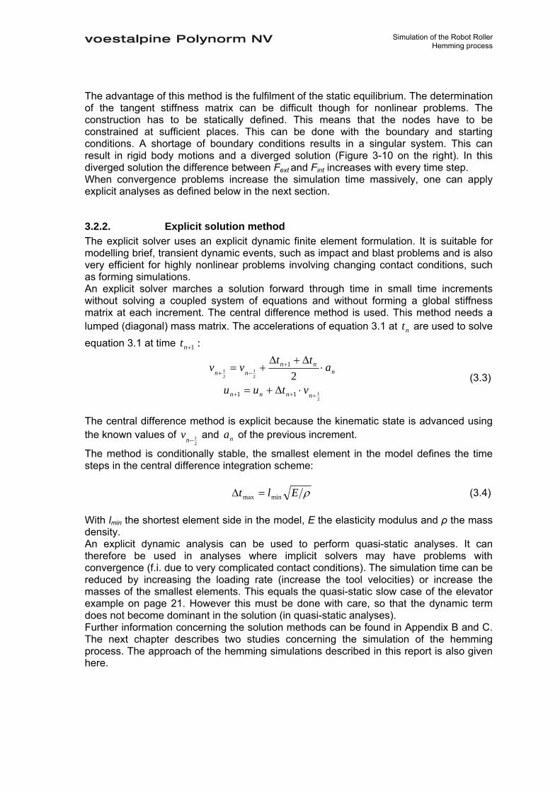
3.2.2. Explicit solution method The explicit solver uses an explicit dynamic finite element formulation. It is suitable for modelling brief, transient dynamic events, such as impact and blast problems and is also very efficient for highly nonlinear problems involving changing contact conditions, such as forming simulations. An explicit solver marches a solution forward through time in small time increments without solving a coupled system of equations and without forming a global stiffness matrix at each increment. The central difference method is used. This method needs a lumped (diagonal) mass matrix. The accelerations of equation 3.1 at nt are used to solve equation 3.1 at time :1+nt
nnn
nn att
vv ⋅Δ+Δ
+= +−+ 2
1
21
21
2111 +++ ⋅Δ+= nnnn vtuu
(3.3)
The central difference method is explicit because the kinematic state is advanced using the known values of
21−nv and na of the previous increment.
The method is conditionally stable, the smallest element in the model defines the time steps in the central difference integration scheme:
ρElt minmax =Δ (3.4) With lmin the shortest element side in the model, E the elasticity modulus and ρ the mass density. An explicit dynamic analysis can be used to perform quasi-static analyses. It can therefore be used in analyses where implicit solvers may have problems with convergence (f.i. due to very complicated contact conditions). The simulation time can be reduced by increasing the loading rate (increase the tool velocities) or increase the masses of the smallest elements. This equals the quasi-static slow case of the elevator example on page 21. However this must be done with care, so that the dynamic term does not become dominant in the solution (in quasi-static analyses). Further information concerning the solution methods can be found in Appendix B and C. The next chapter describes two studies concerning the simulation of the hemming process. The approach of the hemming simulations described in this report is also given here.

Simulation of the Robot Roller Hemming process
4. Simulation of the hemming process The development of the FE-method for simulation of processes in general together with the constantly increasing computer power over the past years has increased its range of applications. Contact between deformable parts became available and highly non-linear problems can now be solved. Two recent papers concerning the simulation of the hemming process are discussed below in section 4.1 (the latest paper became available at the end of this graduation work). The approach of the hemming simulations in this report is described in section 4.2.
4.1. Literature study of hemming simulations In 2003, Sigvant et al. [5] presented his Ph.D. thesis at the Chalmers University of Technology. The first part of his study concentrated mainly on the hemming of flat test panels with straight flanges. Several 2D models have been investigated with different element-types and material models. Both the flanging and hemming operations were simulated. The two main results from these simulations, the roll-in and hemming forces, were then compared with experimental results from hemming experiments. All simulations were made with the explicit code of LS-Dyna®. The second part of his study concentrated on the simulation of all the different manufacturing steps required for the production of an automotive hood. The stamping simulations were made with Autoform® (implicit code) and the flanging and hemming simulations with the explicit code of LS-Dyna®. For this model shell elements were used. The following observations were made: • The 2D simulation results showed a good similarity with experimental results. The
predicted roll-in values are closer to the experimental measurements than the predicted hemming forces. The difference in hemming forces between experiments and simulations was due to the rough approximation of the friction coefficient and the force measurement method used in experiments.
• The similarity between simulations and experiments after prehemming was generally better than the accuracy after final hemming both for solid and shell elements.
The conclusions of the study were: • Shell elements are applicable, although the radius of curvature in the folded area is
of the same order of magnitude as the sheet thickness. • The material parameters investigated, mainly influence the hemming forces.
Differences in roll-in were only small. The second paper was presented at the International Deep Drawing Research Group (IDDRG) congres in Porto, june 2006 [6]. It deals with the simulation of the roll hemming process of an Al-Mg alloy with the implicit code of Abaqus®. During this joining process, planar samples are flanged and then bent in two steps along a curved line with a roller. Special emphasis was given to the influence of constitutive models on numerical predictions. Three different constitutive models were considered: isotropic yield surface with either isotropic or mixed hardening and Hill’ 48 anisotropic yield surface with isotropic hardening. Uniaxial tensile tests and simple shear tests were performed at 0°, 45° and 90° to the rolling direction. A good correlation between experimental and simulated results was seen. These material models were then used in the simulation of

Simulation of the Robot Roller Hemming process
the roll hemming process. The inner and outer blanks were meshed with hexaedrons (solids) with linear interpolation. First the flanging process was simulated. The springback of the flange was taken into account by removing the punch from the part. A two step roll hemming process was then simulated with a support track for the roller included in the hemming anvil (depicted right in Figure 4-1).
Figure 4-1
Two step roll hemming process. Distribution of the equivalent Mises stress is displayed, it reached a maximum of 460 MPa in prehemming (left) and 567 during final hemming (right)
Half of the sample was meshed to decrease the simulation time although the model was not symmetric (movement pattern of the roller is not symmetric) and symmetry conditions were applied at the center of the parts. This assumption is to be removed in a further work to investigate the influence. The influence of different material models on hemming forces and roll-in values was investigated. The following conclusions were made: • Roll-in values do not depend significantly on the material models. • Slight differences were seen depending on the constitutive law whereby the mixed
hardening (both kinematic and isotropic hardening which results in an increasing and shifting yield surface) showed the biggest deviation.
• The load variation during the process showed an irregular peak and these oscillations were believed to be mesh and friction dependent.
In the next section the approach of the hemming simulations is given and explained.
4.2. Approach of the hemming simulations Hemming and sheet metal forming processes in general are considered to be quasi-static manufacturing processes [5]. It can therefore be simulated with the implicit and explicit method. In this work, the finite element software package Abaqus® is used. The hardware is a dual processor (Intel® Xeon 3.06 GHz) computer with 2 GB of internal memory. The difficulties of finite element simulations of hemming lie in material nonlinearities, large local strains near the flange radius of the outer part and the contact with friction between the tools and parts. The changing contact conditions during the hemming process and sheet metal forming simulations in general have limited the use of implicit methods in the past. The studies investigated above concluded that the roll-in values are not influenced significantly by different material models. Only the hemming forces show a significant response. Since the required hemming forces are of less interest not material, but process parameters are varied in this report.

Simulation of the Robot Roller Hemming process
The simulations will be started with a two dimensional model which can simulate the die and tabletop hemming process (chapter 5). The simulations are verified with two references. This model will form the basis for the later 3D robot roller hemming simulation model (defined in chapter 6). The geometry of the hemming process does not fulfil the shell theory. In the hem area the radius of curvature/thickness ratio is too small. However the use of shell elements is necessary to perform hemming simulations in a reasonable time. To investigate the influence of shell and solid elements on the results a three dimensional tabletop model is simulated with different element-types (section 5.2). This way a suitable element for the 3D robot roller hemming simulations is obtained. It is desired to obtain an implicit solution because of the static equilibrium check. If the implicit method has problems with convergence and the solution time is therefore long the explicit method will be applied. The implicit solution is then used as a reference for the explicit solution. This verifies if the use of the explicit method is valid for the simulation of the hemming process.

Simulation of the Robot Roller Hemming process
5. Die and Tabletop hemming simulations The robot roller hemming process can only be simulated with a three dimensional model. This is complex to set up from scratch. There is also no reference situation available to validate the model. The die and tabletop hemming processes are applied a lot. Process information is available. Therefore the die and tabletop hemming processes are first simulated. This can be done with a two dimensional model. By starting with a two dimensional model experience is gained in the simulation of the hemming process. Both implicit and explicit solution methods will be applied to see if the explicit analysis could be applied in a robot roller hemming model. The simulation model is validated by varying process parameters. This 2D model forms the basis for the 3D simulations, different element-types are compared in a three dimensional tabletop simulation to choose an efficient but accurate element-type for the future robot roller hemming simulations. The simulation model development is described in section 5.1. The model is validated with two studies. In section 5.2 the model is transformed to a three dimensional model. Different element-types are compared in the simulation of a tabletop hemming process. The assumptions taken from these simulations and applied on the robot roller hemming model are given in section 5.3.
5.1. 2D simulation model development In this section the 2D model development is described. The developed simulation model is validated with die and tabletop information based on two study cases. The structure of the simulation model is described next. Finally the results (based on different process settings) are compared with the original results of both study cases to validate the model.
5.1.1. Validation information from practice The 2D model will be validated with two studies. The first study was a research project done in the past (1996) by Polynorm Grau [7] concerning the hemming of aluminum test parts. The second study investigated different hemming technologies and was performed at Polynorm Bunschoten [1]. Both these studies are explained first. The results extracted to validate the model are also described here.
Polynorm Grau case – Aluminum Hemming This study deals with the hemming of test parts of aluminum (of the types 5xxx and 6xxx) with the die hemming process. The influence of the hem tooling (pre and final hem tools) on the outcome of the hemming process was investigated. Different geometries of prehem and final hem tools were used which are depicted in Figure 5-1. The tool geometries were based on (see Figure 5-1 below): • Tool radii, R45 for the prehem tool and R2 for the final hem tool • the cutaway length D and depth S of the final hem tool The attack point of the prehem tool 0θ defines the start position for the prehemming step. The tool parameters for both the prehem and final hem tools are depicted in Figure 5-1 on the next page.

Simulation of the Robot Roller Hemming process
Figure 5-1
Tool parameters for the prehem (left) and final hem tool (right); Parameter values are depicted right The parameters which were varied in the study are R45, R2 and S. In Table 5-1 below the variations are given.
Parameter variations [mm] #1 #2 #3 #4 R45 15 35 55 Infinite (straight) R2 2.5 3 3.5 S 1.2 0.6 0.0
Table 5-1 Parameter variations of the Grau case
Two aspects related to the final hem shape were looked at: the roll-in (Figure 2-14) and the warpage (Figure 2-17) of the hem. The influence of the parameters described above on both aspects was plotted in graphs. These graphs are depicted below in Figure 5-2 (depicted left: roll-in, right: warpage). The real roll-in values are not known since the original Grau results (appendix E) were compared with simulation results but their variations are depicted below.
00.10.20.30.40.50.60.70.80.9
0 1 2 3 4 5
Parameter variation #
Rol
l-in
[mm
]
R45 R2 S
00.010.020.030.040.050.060.070.080.090.1
0 1 2 3 4 5
Parameter variation #
War
page
[mm
]
R45 R2 S
Figure 5-2 Result graphs of the Polynorm Grau case; Roll-in results (left), Warpage results (right)
A simulation model with the same tool shape parameters as in the Grau study can be verified with these roll-in results. Only the tool geometries and the deployed alloys are known. The tool displacements are not exactly defined as is the down holding method for the inner part. Also the variation of roll-in is only known. Therefore only a qualitative comparison can be made.
Polynorm Bunschoten case – Hemming basics This second study gives an overview of the different aspects of the hemming process. Available information of car manufacturers and the Polynorm group was analyzed with the objective to better understand different hemming techniques. The die, tabletop and robot roller hemming processes were investigated and the main differences between them were given. Some of this information is presented in chapter 2.

Simulation of the Robot Roller Hemming process
One observation of the study was that there is more roll-in to be expected with a horizontal prehemming step (tabletop hemming) than with a vertical prehemming step (die hemming). This observation can be used to validate a 2D simulation model of both a tabletop and a die hemming installation. A tabletop model should produce more roll-in when the hemming geometry and hemming material are the same for both models. The 2D simulation model is described in the next section.
5.1.2. 2D simulation model The simulation model defined below is suited for an implicit solution method. This is done because an implicit solution will represent a quasi-static solution which is checked on static equilibrium. With minor adjustments the model can be solved with an explicit method. These adjustments are given at the end of this section. The simulation model will be explained below divided into the following parts: • Geometry • Material • Contact • Boundary conditions • Process steps • Friction • Converting the model from implicit to explicit
Geometry Figure 5-3 on the next page illustrates the geometry of the model at the start of the hemming process. The outer and inner parts are assumed to be flat surface parts (depicted above in Figure 5-3). Only a small section of the geometry will be simulated (Figure 5-3, below) because the deformations of the process are very local. The deformable parts are colored orange. Boundary conditions are applied on the right side of the model (BC’s in Figure 5-3) which represent the behaviour of the rest of the structure. This way fewer elements are required which reduces the simulation time. The outer part (lower orange part) rests on a die. The inner part rests on the outer part and is held in place by a downholder and the boundary conditions. With this constraining method the inner part can deform during the analysis.
Figure 5-3
Starting point of the hemming process; Outer and inner part (depicted above) Only a local part of the geometry will be simulated (depicted below)

Simulation of the Robot Roller Hemming process
In Table 5-2 the starting geometry data of both cases is given. The geometry data is depicted in Figure 5-3 above.
Reference studies Polynorm Grau case Hemming Basics case
Material: (Alu 5754 – H22) (Steel DC04) Type of hem: Rope hem Flat hem
Geometry data: Flange height [mm] 15 9
Thickness outer part [mm] 1.25 0.70 Thickness inner part [mm] 1.25 0.70
Inner radius [mm] 1.50 0.50 Gap inner – outer part [mm] 2 2
Table 5-2 Starting geometry of both reference cases
The geometry of both cases differs because different materials were applied in both situations. The aluminum materials applied in the Grau case were not suited for a flat hem shape. This is because the aluminum parts are thicker than the steel parts. A rope hem is required (appendix E) which needs a higher flange to create the rope shape.
Material In the Grau case a 5754-SSF (Stretcher strains free) alloy is used. Stretcher strains are eliminated by a thermo-mechanical treatment. Only the material data of a 5754-H22 alloy (H22: strain hardened and partially annealed to a quarter hard condition) is available. Since the roll-in values do not depend significantly on the material data [5] the use of this material is justified. In the tabletop and die simulations a DC04 deep drawing steel is used. Both materials use an isotropic material model. The stress-strain curves are based on Nadai hardening (which defines the plastic hardening behaviour: ( )nC εεσ += 0 ). The material properties are given below in Table 5-3. The Nadai properties are given under plasticity data.
Material Alu-5754-H22 DC04
Density [kg/dm3] 2.70 7.80 Young’s modulus [MPa] 70*103 210*103
Poisson’s ratio 0.3 0.3 Plasticity data:
0ε 0.00934 0.00846 n 0.22 0.25 C 411 547
Table 5-3 Material properties used in the simulations
The sort of hardening model has a big influence on the results, when Voce hardening is used in stead of Nadai differences of 35 % in roll-in are seen. The Voce model creates the least roll-in. A Voce hardening model assumes that the hardening at higher strain levels is negligible (stress/strain curve remains almost horizontal at high strain levels). This might create a plastic hinge at high deformations (no hardening occurs in the hem area). The material based on the Nadai hardening behaves stiffer which results in more roll-in (there is still some hardening in the model at high deformations). The flange buckles later during the hemming steps.

Simulation of the Robot Roller Hemming process
A good hardening model investigation must therefore be performed for different materials when a quantitative solution is desired.
Contact There are a lot of parts in contact during the hemming process: • Outer part/Die. The outer part rests on a hemming die. • Inner part/Outerpart. The inner part rests on the outer part. At the end of the
hemming process the outer part toughes the inner part to create a hem. • Inner part/Downholder. The inner part is constrained by a downholder. • Outer part/Prehem tool. The prehem tool bends the flange during prehemming. • Outer part/Final hem tool. The final hem tool completes the hemming by bending the
outer part to a hem. These contacts all have the same properties. The contacts defined in the implicit model are based on master and slave surfaces. In Figure 5-4 an example of a master/slave contact combination is given. Nodes of a slave surface (dotted line in the figure) can not penetrate a master surface (continuous line). A master surface can penetrate a slave surface in between their nodes.
Figure 5-4
The master surface can penetrate the slave surface The master surface constrains the slave nodes in a normal direction by a contact pressure, and in a tangential direction by a friction force. The contact pressure and the friction force are defined in the simulations with: • Normal behaviour: Hard contact, separation allowed; The contact pressure is directly applied when penetration of slave nodes through a master surface occurs (depicted left in Figure 5-5 where the horizontal axis represents the clearance between two components and the vertical axis the contact pressure when two components are in contact). Any contact pressure is possible when the surfaces are in contact. • Tangential behaviour: Penalty method; The amount of sliding between components is dependent on the contact pressure and the friction coefficient μ (depicted right in Figure 5-5, μ defines the steepness of the graph). If the shear stress arising from contact between two components is higher than the critical shear stress for a certain contact pressure, sliding of surfaces occurs. This is the case if the shear stress is higher than the left curve of Figure 5-5.

Simulation of the Robot Roller Hemming process
Figure 5-5
Default pressure-overclosure relationship: hard contact (left) and the frictional behaviour based on the penalty method (right)
The influence of the friction coefficient on the roll-in of the hem is described at the end of this section with a set of simulations. This is found on page 31.
Boundary conditions Only a small section of the parts is drawn with boundary conditions applied to the cut-off ends of the right side. The complete outer and inner parts are depicted in Figure 5-3 above on page 24. In Figure 5-6 the remaining model is given. The orange outer and inner parts are deformable parts and the tools (die and downholder) are rigid. The deformations are very local and the cut-off ends of both parts are assumed to remain in place. This reduces the amount of elements required to simulate the model which decreases the simulation time.
Figure 5-6 The boundary conditions applied on the right side of the model; Both applied at the inner and outer part
The following boundary conditions are applied in the model: • Symmetry on the right side of the model (applied on both the inner and outer part); x-
displacement (Ux), y-displacement (Uy) and z-rotation (Rz) are zero. The z-axis is perpendicular to the plane of the drawing. The symmetry conditions can be applied far from the symmetry axis of the parts because the deformations are very local.
• The die is fully constrained; x-, y-displacement and z-rotation = 0. • The downholder of the inner part is fully constrained; x-, y-displacement and z-
rotation = 0. The downholder is applied on the sloped section of the inner part. The inner part can still buckle/move during hemming. The steps required to simulate the process are described below.
Process steps The hemming process is divided into a prehemming and a final hemming step (see section 2.2). Before the hemming process is performed a flange has to be created in a

Simulation of the Robot Roller Hemming process
flanging process (see Figure 2-4). This is simulated before the hemming because it is expected that the flanging process has a significant effect on the roll-in results. This is due to its hardening effect in the corner of the flange. The process steps will be explained below divided into the three main steps: flanging, prehemming and final hemming. Flanging The edge of the outer part which is to be hemmed is created with the flanging process. The flanging process is depicted in Figure 5-7 below. An outer part is clamped between a blankholder and a die. A punch is moved downwards to bend the flange (punch radius = 1.5 mm and the flanging die radius equals the desired inner radius of the outer part (given next to Figure 5-7 on the next page)):
Alu 5754-H22 Steel DC04
Flanging die radius [mm] 1.5 0.5
Figure 5-7 The flanging process (schematically); The flange is created by moving a punch downwards
In the simulation the flanging process is performed upside down. This has no effect on the results. The rigid tools of the simulations used in the flanging process are named in Figure 5-8. These tools can be moved during the process in two ways: by applying a force or prescribing a displacement. These conditions are applied to the reference points of the tools (crosses in Figure 5-8). The flanging process is divided in two small steps in the simulation (Both depicted in Figure 5-8). The simulation starts by applying a small force to the blankholder which clamps the outer part between the blankholder and the die (left figure).
Figure 5-8
Step 1: Apply holder force (left); Step 2: Move the punch (right) The force has to create a small pressure on the blank which constrains it during the flanging and hemming process. The Mises stress induced by this force on the outer part is equal to 10 MPa. Now that the outer part is clamped the flange can be created (Figure 5-8 on the right). The punch is moved vertically to create the flange. This is done by prescribing a displacement in the y-direction (equal to the flange height). The future hem is influenced by this flanging process. The equivalent plastic strain distribution after the flanging process (extracted from simulations) is given below in Figure 5-9. The mechanism of the roll-in is influenced by this strain distribution.

Simulation of the Robot Roller Hemming process
Figure 5-9
The equivalent plastic strain distribution after the flanging process; Areas where a lot of deformation occurred are colored red, the blue areas are undeformed
For the aluminum geometry a maximum equivalent plastic strain of approximately 0.30 is located in the corner of the flange (red area in Figure 5-9). For the steel geometry the equivalent plastic strain is even higher, approximately 0.50. The material located outside this strengthened area is expected to deform first. The material will either deform in the flange (vertical area in Figure 5-9) or in the panel (horizontal area in Figure 5-9). There are three possibilities for the amount of roll-in: • Roll-out, only the flange deforms. The hem radius develops in the flange area. • Maximum roll-in, only the panel deforms. The hem radius develops in the panel. • A combination of both, deformation in the panel and in the flange. The hemming tools and applied hemming method will determine the working of this roll-in mechanism. This was one of the reasons for the Grau investigation. Next the prehemming step is explained. Prehemming In the prehemming step the opening angle of the flange is reduced from 90° to 45°. The outer part is clamped between the hemming die and the inner part. The inner part itself is held in place with a downholder. Different downholder shapes and positions are used in practice. In the 2D model simulations a downholder is placed on the sloped area of the inner part (see Figure 5-3). First the blankholder of the flanging process is removed and the interaction between the inner part and outer part is created. This results in little buckling of the outer part (it is now only constrained by the inner part, Figure 5-10 on the left). The inner part itself is constrained by its own downholder.
Figure 5-10
Step 3: Original downholder removed and inner part introduced (left); Step 4: The punch is removed, this is the start of the hemming process
The punch has to be removed before the hemming steps can take place (Figure 5-10, right). Note that the flange shows some springback. The flange is slightly angled to the left. This is the start of the prehemming step (Figure 5-11).

Simulation of the Robot Roller Hemming process
Figure 5-11
Step 5: Prehemming step The prehemming step is performed by displacing the prehem tool downwards (prescribed displacement). This is done till the flange is bend ± 45°. The prehemming tool is removed before the final hemming step can take place (displaced upwards, which results in a little springback of the flange, the flange bends slightly to the left). Final hemming During the final hemming step the opening angle of the flange is decreased from 45° to 0°. This process completes the hemming. In the simulation model the final hemming is performed by prescribing a displacement to the final hem tool. The final hem tool moves down to create a hem with a thickness three times the blank thickness.
Figure 5-12
Step 6: final hemming The original position of the final hem tool at the beginning of the final hemming step is not described in the Grau study and is assumed as follows. During the prehemming step the flange will roll-in. This amount of roll-in is decreased during the final hemming step. The flange must have space to roll-out during final hemming. The gap between the final hem tool and the hem during the final hemming step (Figure 5-12, the gap between the vertical line of the final hem tool and the outer edge of the hem) determines this space. After the hemming process the gap is decreased (see Figure 5-13). This means that roll-out has occurred in the last phase of the final hemming step. The best rope hem is acquired if the gap is reduced to zero after final hemming step. This way the hem develops in the cut-away of the final hem tool. This final hem tool position is defined with the help of previous simplified trial and error simulations.
Figure 5-13
End position of step 6 After the simulation the shape of the hem, the amount of roll-in and the stress/strain distribution can be analysed. Before these results can be analysed, a correct amount of friction has to be defined.

Simulation of the Robot Roller Hemming process
Friction Friction is an important factor in simulations. It influences the force/displacement characteristics of tools as well as the local strains and the strain distribution [8]. The amount of friction is defined by the friction coefficient μ. The friction coeffient is expected to have a big influence on the results because: • the contact pressures are high during the hemming steps (especially final hemming,
see Figure 5-12 on page 35 where the flange is pressed together) • there are a lot of components in contact during the simulation Assumed is that the friction coefficient is constant for all the components interacting (both for steel and aluminum). The contact pressure is, in combination with the friction coefficient, defining the stick/slip behaviour of two components. A set of simulations with different friction coefficients shows the influence on the roll-in of the hem (simulations are based on the Grau study). In Table 5-4 the results are depicted.
Results from the implicit simulations [R45 = 15, R2 = 2.5 and S = 1.2 mm] Friction coefficient μ Roll-in after prehemming [mm] Roll-in after final hemming [mm] 0.00 0.69 0.92 0.05 0.61 0.57 0.10 0.50 0.41 0.15 0.39 0.30 0.20 0.31 0.26 0.30 0.19 -0.05* 0.40 0.11 -0.39* 0.50 0.08 -0.82*
Table 5-4 Roll-in after pre- and final hemming (simulations with different friction coefficients, implicit)
*negative roll-in values represent roll-out The roll-in values depicted in Table 5-4 are total roll-in values. In practice hemming simulations show the following roll-in behaviour: • During prehemming the flange rolls in. This should give positive roll-in values. • After final hemming roll-out occurs. The amount of roll-in should be decreased in the
final hemming step (based on die and tabletop hemming experience). The total amount of roll-in is still positive though. The outer part is decreased in size.
The results of Table 5-4 are plotted in Figure 5-14 below. The vertical axis represents the roll-in, the horizontal axis the friction coefficient. The blue line shows the roll-in value after prehemming, the red line after final hemming.

Simulation of the Robot Roller Hemming process
-1-0.8-0.6-0.4-0.2
00.20.40.60.8
11.2
0 0.1 0.2 0.3 0.4 0.5
Frictioncoefficient
roll-
in [m
m]
roll-in after final hemming roll-in after pre-hemming
Figure 5-14
Roll-in after pre- and final hemming (simulations with different friction coefficients, implicit) No roll-out during final hemming occurs at friction levels below μ = 0.05. With too much friction (μ > 0.30) total roll-out occurs (the outer part is increased in size). This is very unlikely in practice. So 0.05 ≤ μ ≤ 0.30. The area between the coefficient-range of 0.15 to 0.20 has little influence on the roll-in after final hemming. For deep draw simulations in Autoform® a value of 0.17 is used for aluminum materials. This value is chosen for the 2D simulation model. The implicit 2D simulation model is defined now. The larger future 3D simulation model might require too much simulation time. The explicit solution method might be more efficient. To investigate if hemming simulations can be performed with the explicit solution method, the 2D simulation model is converted. Several changes are needed and are explained below. Converting the model from implicit to explicit The simulation model described above is based on an implicit model. No masses have to be defined. Tool displacements are addressed to the tools. The implicit method is then defining the tool speeds and is thereby taking care that a quasi-static solution is found. If the implicit model is having trouble finding a solution due to nonlinearities (see chapter 3 page 19) or if the solution takes a lot of time to obtain, one can apply the explicit method. In an explicit analysis masses and time need to be defined. A solution is found in very small timesteps (increments). This is done by calculating the accelerations of the parts based on the known speeds and accelerations from the previous increment. The accelerations are calculated with the help of a lumped mass matrix. The masses of the inner and outer part are defined by the density of the material. Since the explicit solver can not solve the problem with no mass, a point mass has to be added to the reference point of the rigid tools. This way a force can be applied. A point mass is therefore applied to the blankholder. This way the blankholder can clamp the outer part for the flanging process. This mass is not related to the real mass of the downholder but it has to be in the same order as the mass of the outer part which it constrains. The value of the clamp force is therefore different than in the implicit model but the Mises stress is still 10 MPa so the results are not influenced by this change. The other tools have only displacements related to them, no forces. Therefore no mass is given to them. But since the accelerations of the tools are required real time steps need to be defined. The tool velocities of all the tools are based on a realistic value of the punch speed (100 mm/s). The simulation time can be reduced in two ways in the explicit method without degrading the quality of the simulation a lot: increasing the tool velocities (load scaling) or
Simulation of the Robot Roller Hemming process
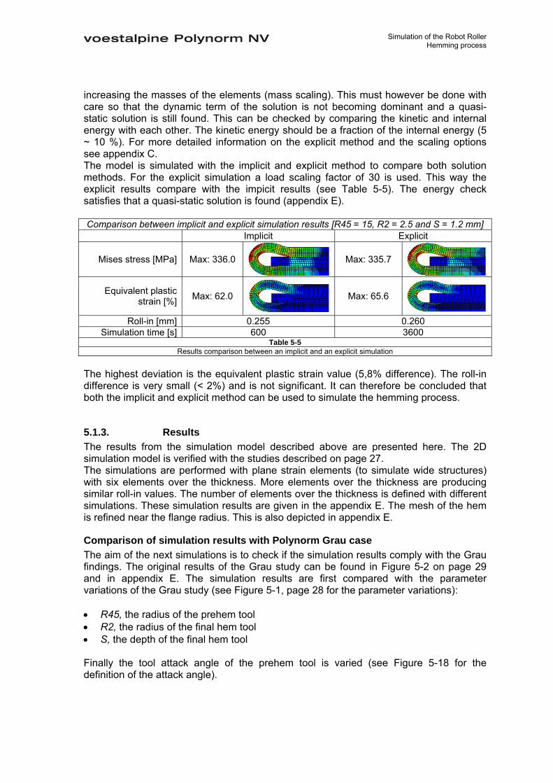
increasing the masses of the elements (mass scaling). This must however be done with care so that the dynamic term of the solution is not becoming dominant and a quasi-static solution is still found. This can be checked by comparing the kinetic and internal energy with each other. The kinetic energy should be a fraction of the internal energy (5 ~ 10 %). For more detailed information on the explicit method and the scaling options see appendix C. The model is simulated with the implicit and explicit method to compare both solution methods. For the explicit simulation a load scaling factor of 30 is used. This way the explicit results compare with the impicit results (see Table 5-5). The energy check satisfies that a quasi-static solution is found (appendix E). Comparison between implicit and explicit simulation results [R45 = 15, R2 = 2.5 and S = 1.2 mm]
Implicit Explicit
Mises stress [MPa] Max: 336.0 Max: 335.7
Equivalent plastic strain [%] Max: 62.0 Max: 65.6
Roll-in [mm] 0.255 0.260 Simulation time [s] 600 3600
Table 5-5 Results comparison between an implicit and an explicit simulation
The highest deviation is the equivalent plastic strain value (5,8% difference). The roll-in difference is very small (< 2%) and is not significant. It can therefore be concluded that both the implicit and explicit method can be used to simulate the hemming process.
5.1.3. Results The results from the simulation model described above are presented here. The 2D simulation model is verified with the studies described on page 27. The simulations are performed with plane strain elements (to simulate wide structures) with six elements over the thickness. More elements over the thickness are producing similar roll-in values. The number of elements over the thickness is defined with different simulations. These simulation results are given in the appendix E. The mesh of the hem is refined near the flange radius. This is also depicted in appendix E.
Comparison of simulation results with Polynorm Grau case The aim of the next simulations is to check if the simulation results comply with the Grau findings. The original results of the Grau study can be found in Figure 5-2 on page 29 and in appendix E. The simulation results are first compared with the parameter variations of the Grau study (see Figure 5-1, page 28 for the parameter variations): • R45, the radius of the prehem tool • R2, the radius of the final hem tool • S, the depth of the final hem tool Finally the tool attack angle of the prehem tool is varied (see Figure 5-18 for the definition of the attack angle).

Simulation of the Robot Roller Hemming process
Prehem tool radius R45 The influence of the prehem tool radius R45 is investigated. See Table 5-6 and Figure 5-15 below for the simulation results. The results from both solution methods are roughly the same. A difference with the Grau results can be seen for R45 = 55 mm.
Influence of the prehem tool radius on the amount of roll-in [R2 = 2.5 mm; S = 1.2 mm] R45 [mm]: Implicit, roll-in [mm] Explicit, roll-in [mm] 15 0.26 0.26 35 0.91 0.89 55 1.21 1.21 Infinite (straight shape angled 45°) 1.03 1.04
Table 5-6 Roll-in values for different values of R45
The opening angle after prehemming was bigger than 45 degrees for R45 = 55 mm in the Grau study (this in contrary with other values of R45). In the simulations the opening angle after prehemming was always 45 degrees.
0
0.2
0.4
0.6
0.8
1
1.2
1.4
15 35 55 99
R45 [mm]
roll-
in [m
m]
Implicit Explicit Grau Results
Figure 5-15
Influence of the prehem tool radius R45 (left) on the amount of roll-in; The opening angle of the flange after prehemming (right)
A bigger opening angle is a result of a smaller prehem tool displacement. See Figure 5-15 on the right for the different opening angles (the orange outer part has a bigger opening angle than the blue outer part). Less roll-in is created with a bigger opening angle (the orange outer part in Figure 5-15 on the right has less roll-in than the blue outer part). And with a bigger opening angle the flange buckles earlier during final hemming. This all results in less roll-in and is a reason for the difference with the Grau results at R45 = 55 mm. Final hem tool radius R2 The radius of the final hem tool R2 is varied (by changing the radius the length of the opening in the final hem tool is also changed, D in Figure 5-1 on page 28 above). Assumed is that D = 2*R2. See Table 5-7 and Figure 5-16 for the results.
Influence of the final hem tool radius on the amount of roll-in [R45 = 15 mm; S = 1.2 mm] R2 [mm]: Implicit, roll-in [mm] Explicit, roll-in [mm] 2.5 0.26 0.26 3.0 0.29 0.31 3.5 0.47 0.48
Table 5-7 Roll-in values for different values of R2

Simulation of the Robot Roller Hemming process
With a bigger value of R2, the flange gets more room to move into the depth of the final hem tool. This is because it was assumed that the value of D also varies with R2 (D = 2*R2). In Figure 5-16 on the right the two extreme values of R2 are depicted. In the lower figure the hem develops more in the final hem tool and a better rope hem is acquired. While interpreting these simulation results it is concluded that no dependent D is used in the Grau R2 variations. Therefore no kink is seen in their results.
00.050.1
0.150.2
0.250.3
0.350.4
0.450.5
2.5 3 3.5
R2 [mm]
roll-
in [m
m]
Implicit Explicit Grau Results
Figure 5-16 Influence of the final hem tool radius R2 (left) on the amount of roll-in; Extreme values of R2 (right)
Finally the influence of the final hem tool depth S is simulated. See Table 5-8 and Figure 5-17 below.
Influence of the final hem tool depth on the amount of roll-in [R45 = 15 mm; R2 = 2.5 mm] S [mm]: Implicit, roll-in [mm] Explicit, roll-in [mm] 0.0 0.34 0.33 0.6 0.28 0.28 1.2 0.26 0.26
Table 5-8 Roll-in values for different values of S
In this graphs a small kink is seen also (this time both in the Grau and simulation results). In Figure 5-17 on the right the result shapes of different tool depths S are depicted. With S = 1.2 mm (above figure) the flange does not move through the total height of S. With S = 0.6 mm (middle figure) the flange deforms more in the depth of the final hem tool. With S = 0 mm (lower figure) the flange has no space to deform in the final hem tool which results in a flat hem. The kink is created because two rope hems and one flat hem are compared on roll-in. When three rope hems are compared the graph would probably be straight. The results from the Grau study are extremer which also indicates that a bigger value of D is used in the simulations. This also complies with the fact that no kink is seen in the Grau graph of the R2 variations (Figure 5-16 above).

Simulation of the Robot Roller Hemming process
00.050.1
0.150.2
0.250.3
0.350.4
0 0.6 1.2
S [mm]
roll-
in [m
m]
Implicit Explicit Corus Reference
Figure 5-17
Influence of the final hem tool depth S on the amount of roll-in (left); All result values of S (right) Now all the simulation and Grau results are compared on roll-in. The simulation results comply with them qualitatively which can be slightly improved with a bigger value of D in all simulations which is not depending on the value of R2. Since this process type investigation does not have the highest priority this is left undone. Prehem tool attack angle The influence of the prehem tool attack angle (see Figure 5-18 for the definition of the attack angle) should be small around °= 350θ . This is because the Grau investigation is based on real die hem process settings. In practice after several process cycles 0θ might change slightly caused by wear of the installation. This may not have a significant influence on the roll-in of the product.
Figure 5-18
Prehem tool attack angle 0θ ; definition (left), 15° (middle) and 60° (right)
The influence of the attack angle is checked with the following angles: 15°, 30°, 35°, 40°, 45°, 60° (steps of 15° for the big influence and 5° above and below 35° to investigate the process certainty). To illustrate the definition of the prehem tool attack angle, the result of 15° and 60° are depicted in Figure 5-18 above. The results are given below:
0
0.2
0.4
0.6
0.8
1
1.2
1.4
0 20 40 60 80
Tool attackpoint [degrees]
roll-
in [m
m]
roll-in after pre-hemming roll-in after final hemming
Figure 5-19
Influence of the prehem tool attack point on the roll-in

Simulation of the Robot Roller Hemming process
As can be seen in Figure 5-19 the influence around the prescribed attack angle is negligible (roll-in values of around 0.75 mm from 30°< 0θ <45°). The attack angle has therefore probably no influence on the process certainty because it is unlikely that the attack angle changes more than 5° (5° corresponds to a 1 mm shifted tool or product). The highest amount of roll-in is seen at 15°. This is a result of the sliding of the flange along the prehem tool. With the highest attack angle of 60° the flange buckles earlier during the prehemming and the roll-in is therefore decreased compared to lower attack angles.
Comparison of simulation results with Polynorm Bunschoten case A die and tabletop hemming variant are compared whereby the only difference between both processes is the movement direction of the prehemming step (a vertical movement for die hemming and horizontal movement for tabletop hemming, see Figure 2-7 and Figure 2-10 above on pages 11 and 12). This simulation model is similar to the model based on the GRAU study with the difference that steel (DC04, deep drawing steel) is used in stead of aluminum. Therefore the final hem tool is changed because no rope hem is required in steel. A flat hem is now the outcome of the hemming process. See Table 5-2 on page 30 for the changes in the geometry of the parts. In the die hemming variant the prehem tool moves vertical, for the tabletop variant the prehem tool moves horizontal. The results from the two simulations are given below in Table 5-9. Both processes are simulated with the implicit simulation method.
Influence of the process type on the amount of roll-in
roll-in total [mm] after pre-hemming
roll-in total [mm] after final hemming
roll-in [mm] final hemming
Die hemming 0.71 0.57 -0.14 (roll-out) Tabletop hemming 0.82 0.68 -0.14 (roll-out)
Table 5-9 roll-in values with different process types
As can be seen in Table 5-9 the difference in roll-in is created in the prehemming step. The final hemming step produces the same amount of roll-out (-0.14 mm) for both processes. As was expected from the Hemming Basics reference the tabletop process is producing more roll-in during the pre-hemming step. With this 2D simulation model a good basis has been made for the 3D model development. In the next section a 3D model which can simulate a tabletop process is presented. This model is used for an element-type comparison. Finally an element-type for the 3D robot roller hemming model is chosen.
5.2. Influence of element-types on the results of a tabletop simulation As described in chapter 3 two families of element-types are available for the simulation of the hemming process: solid and shell elements. In Abaqus® two types of shells are available: conventional shell elements and continuum shell elements. These shell elements are more efficient in hemming simulations than solid elements. This is because a solution is found with less degrees of freedom than with solid elements would be required. However, the geometry of a hem does not fulfil the shell theory. In the hem area the radius of curvature/thickness ratio (Rinner/touter, see Table 5-2 and Figure 5-3) is too small for the shell theory to hold (Rinner/touter must be approximately greater or equal to five [9]).
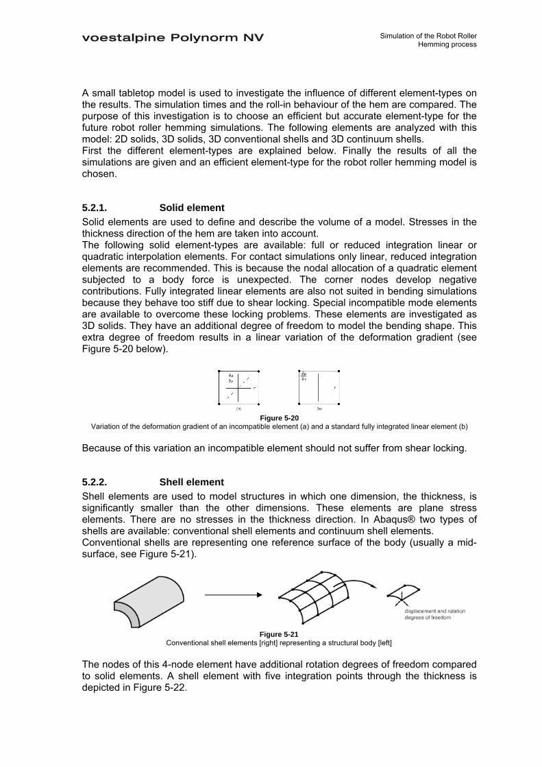
Simulation of the Robot Roller Hemming process
A small tabletop model is used to investigate the influence of different element-types on the results. The simulation times and the roll-in behaviour of the hem are compared. The purpose of this investigation is to choose an efficient but accurate element-type for the future robot roller hemming simulations. The following elements are analyzed with this model: 2D solids, 3D solids, 3D conventional shells and 3D continuum shells. First the different element-types are explained below. Finally the results of all the simulations are given and an efficient element-type for the robot roller hemming model is chosen.
5.2.1. Solid element Solid elements are used to define and describe the volume of a model. Stresses in the thickness direction of the hem are taken into account. The following solid element-types are available: full or reduced integration linear or quadratic interpolation elements. For contact simulations only linear, reduced integration elements are recommended. This is because the nodal allocation of a quadratic element subjected to a body force is unexpected. The corner nodes develop negative contributions. Fully integrated linear elements are also not suited in bending simulations because they behave too stiff due to shear locking. Special incompatible mode elements are available to overcome these locking problems. These elements are investigated as 3D solids. They have an additional degree of freedom to model the bending shape. This extra degree of freedom results in a linear variation of the deformation gradient (see Figure 5-20 below).
Figure 5-20
Variation of the deformation gradient of an incompatible element (a) and a standard fully integrated linear element (b) Because of this variation an incompatible element should not suffer from shear locking.
5.2.2. Shell element Shell elements are used to model structures in which one dimension, the thickness, is significantly smaller than the other dimensions. These elements are plane stress elements. There are no stresses in the thickness direction. In Abaqus® two types of shells are available: conventional shell elements and continuum shell elements. Conventional shells are representing one reference surface of the body (usually a mid-surface, see Figure 5-21).
Figure 5-21
Conventional shell elements [right] representing a structural body [left] The nodes of this 4-node element have additional rotation degrees of freedom compared to solid elements. A shell element with five integration points through the thickness is depicted in Figure 5-22.

Simulation of the Robot Roller Hemming process
Figure 5-22
Section points of a reduced integration 4 node shell element [Simpson’s integration rule] A continuum shell element defines a three dimensional body with two surfaces in stead of one (see Figure 5-23). This makes it easier to define contact between parts (both sides of the part have a surface). Also thickness changes can be simulated.
Figure 5-23
Continuum shell elements [right] representing a structural body [left] Continuum shells are modelled as solids and they also have displacement degrees of freedom only. Their constitutive behaviour is similar to conventional shell elements. They can be stacked for a better thickness response (stacking means more elements through the thickness). Only linear reduced elements are available. A simple simulation model is set up for hemming an outer part with inner part. The result is a flat hem. The hemming material is a deep drawing steel (DC04). The hemming method is based on a tabletop variant with a horizontal pre- and a vertical final hemming movement pattern (see Figure 2-10 on page 12 for the hemming steps). The flanging step is included in the analysis. The geometry of the inner part is changed which also results in a different downholder of the inner part. The differences with the geometry used in the Hemming Basics simulations are depicted in Figure 5-24. This geometry is changed because the robot roller hemming geometry is based on the new geometry. The new inner part is smaller and no sloped area is seen. This is resulting in fewer elements than the Hemming Basics model depicted left. This should reduce the simulation time, especially for the future robot roller hemming model. The position of the downholder is also changed, the downholder is moved 2 mm closer to the flange (distance is now 15 mm).
Figure 5-24
Geometry of the new Tabletop hemming model (left) and the Hemming Basics model (right) The contacts and the boundary conditions applied are similar to the 2D model described in section 5.1.2. Only the normal behaviour of the interaction property is changed from
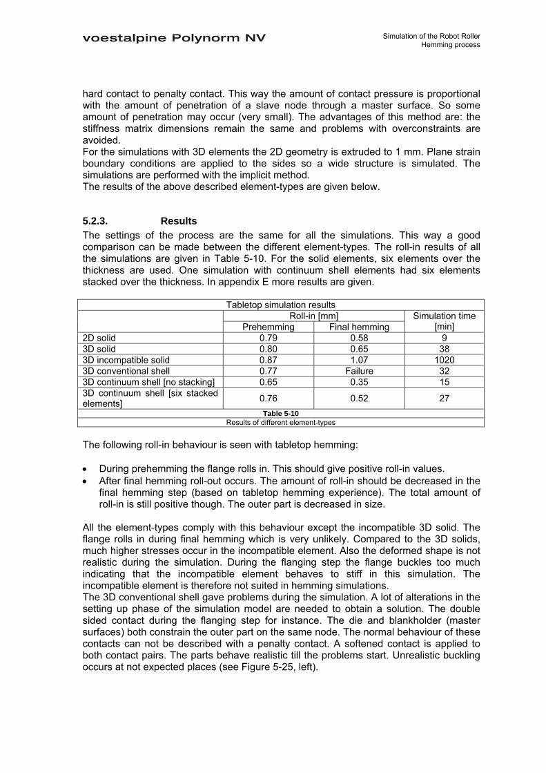
Simulation of the Robot Roller Hemming process
hard contact to penalty contact. This way the amount of contact pressure is proportional with the amount of penetration of a slave node through a master surface. So some amount of penetration may occur (very small). The advantages of this method are: the stiffness matrix dimensions remain the same and problems with overconstraints are avoided. For the simulations with 3D elements the 2D geometry is extruded to 1 mm. Plane strain boundary conditions are applied to the sides so a wide structure is simulated. The simulations are performed with the implicit method. The results of the above described element-types are given below.
5.2.3. Results The settings of the process are the same for all the simulations. This way a good comparison can be made between the different element-types. The roll-in results of all the simulations are given in Table 5-10. For the solid elements, six elements over the thickness are used. One simulation with continuum shell elements had six elements stacked over the thickness. In appendix E more results are given.
Tabletop simulation results Roll-in [mm] Prehemming Final hemming
Simulation time [min]
2D solid 0.79 0.58 9 3D solid 0.80 0.65 38 3D incompatible solid 0.87 1.07 1020 3D conventional shell 0.77 Failure 32 3D continuum shell [no stacking] 0.65 0.35 15 3D continuum shell [six stacked elements] 0.76 0.52 27
Table 5-10 Results of different element-types
The following roll-in behaviour is seen with tabletop hemming: • During prehemming the flange rolls in. This should give positive roll-in values. • After final hemming roll-out occurs. The amount of roll-in should be decreased in the
final hemming step (based on tabletop hemming experience). The total amount of roll-in is still positive though. The outer part is decreased in size.
All the element-types comply with this behaviour except the incompatible 3D solid. The flange rolls in during final hemming which is very unlikely. Compared to the 3D solids, much higher stresses occur in the incompatible element. Also the deformed shape is not realistic during the simulation. During the flanging step the flange buckles too much indicating that the incompatible element behaves to stiff in this simulation. The incompatible element is therefore not suited in hemming simulations. The 3D conventional shell gave problems during the simulation. A lot of alterations in the setting up phase of the simulation model are needed to obtain a solution. The double sided contact during the flanging step for instance. The die and blankholder (master surfaces) both constrain the outer part on the same node. The normal behaviour of these contacts can not be described with a penalty contact. A softened contact is applied to both contact pairs. The parts behave realistic till the problems start. Unrealistic buckling occurs at not expected places (see Figure 5-25, left).

Simulation of the Robot Roller Hemming process
Figure 5-25
Unstable behaviour of the conventional shell element at the end of the final hemming A static riks step is a step special for unstable behaviour, but this did not solve the problem. For hemming simulations this element is not suitable because of its unstable behaviour. The 3D linear reduced solids and continuum shells are suited for hemming simulations. The deviations with the 2D plane strain solid are smaller after prehemming than after final hemming. The highest deviations are seen with the continuum shell element with no stacking applied.
5.3. Conclusions The die and tabletop hemming processes can be simulated with a 2D simulation model. Both implicit and explicit solution methods can be applied. Qualitative judgements can be made to a certain amount. The limitations of the 2D model are the low stiffness of the panels. The inner part buckles a lot during some simulations. In practice the panels are probably stiffer due to hardening effects induced by the stamping operation which is neglected here and, in most cases, the 3D geometry of the parts. But despite the flexibility of the panels, similar influences like described in the Grau and Hemming Basics study are found. The low influence of the attack angle of the prehem tool also indicates the validity of the model. In practice a slightly changed attack angle due to wear of the installation should not produce different part dimensions. The processed material needs to be defined accurately when a more quantitative solution is desired. Differences of 35 % in results are seen when Nadai hardening is compared to Voce hardening. The Nadai hardening model is used since this model still gives little hardening at high deformations. At high deformations the Voce model creates a plastic hinge in the hem area because no more hardening occurs. This results in less roll-in. The continuum shell element is best suited for time efficient robot roller hemming simulations. The simulations with this element are representing a realistic shape of the parts during the hemming process. Roll-in is seen after the pre-hemming step and this amount of roll-in is reduced after the final hemming step. The elements can be stacked over the thickness to increase the accuracy. The linear reduced 3D solid element is also suited for simulating the hemming process. The deviations with the 2D solid plane strain element are smaller. The simulation times are only increased compared to the continuum shell element. The incompatible 3D solid element behaves too stiff during the simulation and is therefore not suited. The conventional shell element is not suited for efficient hemming simulations. The implicit model gave a lot of problems at the end of the simulation. Unstable buckling occurs. Interaction properties between tools have to be changed to a softened contact for some contact pairs. This might influence the results slightly. The deviations of all the 3D elements compared with the 2D solid plane strain element were smaller after prehemming than after final hemming. It is desired to obtain an implicit (quasi-static) solution of the hemming process. This way the results can be used as a reference to set up an explicit model which might be faster if a large 3D model is simulated. This explicit model can then be used in a parameter study. The 3D robot roller hemming model is given in the next chapter. A parameter study based on a ‘Design of Experiments’ is given in chapter 7.

Simulation of the Robot Roller Hemming process
6. Robot Roller hemming simulations In this chapter a 3D model for simulating the robot roller hemming process is presented. For the first simulations the three step robot roller hemming process as conducted at Polynorm is taken as a basis. This means hemming a flanged outer part (with a 90° opening angle) in three hemming steps (see Figure 2-5 and Figure 2-12 on pages 10 and 13). Before this simulation model can be made, the practice situation is discussed first in section 6.1. The simulation model development is given in section 6.2. Here is defined which model is to be used in a parameter study.
6.1. Situation in practice First the setup of the process is described in 6.1.1. The parameters specific for the robot roller hemming process are given in 6.1.2. The parameter settings during a three step robot roller process are described at the end of this section.
6.1.1. Set up of the robot roller hemming process The process of setting up a robot roller hemming process can be divided into off- and online programming. The setup process starts with the offline phase. The offline programming consists in creating curves for the robot path. These curves are based on the CAD data of the hemming bed geometry. This data can be converted into the robot program. In the online programming phase a robot is used to set up a process for future production (in a try-out cell) and to perform the process in production. The curves based on the hemming bed geometry of the product are equal to the hemming bed edge. This edge is the target point for the roller and is called the Robot Target Point (RTP). This point should be aligned with a point on the roller called the Tool Center Point (TCP). In Figure 6-1 on the left these points are depicted. This TCP contains a local coordinate axis of the roller (Figure 6-1, right). The x-axis of the local coordinate system aligns with the curves of the hemming bed. The TCP is located about 10 mm (for an outer part with a 9 mm flange) from the top along the edge of the roller. The distance from the top is depending on the flange height.
Figure 6-1 Tool Center Point and Robot Target Point align (left); Local coordinate axis of the main roller types (right)
The distance between the TCP and the RTP is an important parameter of the robot roller hemming process which is described in the section below.

Simulation of the Robot Roller Hemming process
6.1.2. Specific robot roller hemming parameters In this section the robot roller hemming process is described. Starting point for the process is a steel outer part with a flange opening angle of 90° and a flange height of 9 mm. First the specific robot roller hemming parameters are given. Finally the (standard) three step robot roller hemming process is described. Parameters of the robot roller hemming process The parameters are first described by the degrees of freedom of the roller. After that other important specific robot roller hemming parameters are given. The degrees of freedom of the roller are described with the help of Figure 6-2 below. A coordinate axis is placed on the center of the roller.
Figure 6-2
Coordinate axis in the center of the roller, used to describe the degrees of freedom of the roller The parameters which determine the result of the robot roller hemming process are: • The x-axis is parallel with the product and the x-direction is the movement direction of
the roller during the hemming steps. The roller strikes the flange at the top of the flange. This y position of the roller is defined by the TCP which is located 10 mm from the top of the roller (see also Figure 6-1, left). This way the flange (flange height is 9 mm in this case) is always touched at the top of the flange.
• The z-displacement of the roller before actual the hemming step. This can be defined as the TCP – RTP distance (see Figure 6-3, right). The TCP aligns with the RTP (see also Figure 6-1, the TCP and RTP lie on one line perpendicular to the roller). This step defines the initial deformation of the flange before the hemming steps starts. During the hemming steps this distance remains constant.
Figure 6-3
TCP – RTP distance • The orientation of the roller (θ in Figure 6-3 and the rotation around the x-axis of
Figure 6-2). This angle defines in how many steps the outer part is being hemmed. Standard robot roller hemming processes hem products in three steps (θ = 60° for the first step and θ = 30° for the second step). Two step robot roller hemming is in development nowadays (θ = 45°).
• The lead angle of the roller (β in Figure 6-4 and the rotation around the z-axis of Figure 6-2).

Simulation of the Robot Roller Hemming process
Figure 6-4
Lead angle of the roller • A driven or a non-driven roller (rotation α around the y-axis). In most processes the
roller can rotate freely around the y-axis of Figure 6-2 during the hemming step. A non-driven roller is also used within Polynorm.
All six degrees of freedom of the roller are described now. Other parameters specific of the robot roller hemming process are: • The roller size, the diameter of the roller has an effect on the amount of deformation
in the flange. • The roller types, cone shape rollers also have an effect on the amount of deformation
of the flange. In Figure 6-5 two cone shape rollers are depicted.
Figure 6-5
A cone (left) and anti-cone (right) shaped roller • Hemming speed, the speed in the x-direction of Figure 6-2. At straight sections
hemming speeds of 500 mm/s are used. Lower speeds are required in corner sections.
Three step robot roller hemming process The three step robot roller hemming process starts with an outer part with an opening angle of 90°. This is hemmed in three steps by changing the orientation θ of the roller. In the first prehemming step θ = 60°, in the second prehemming step θ = 30°. The orientation of the roller θ is equal to 0° in the final hemming step. The initial bending of the flange happens before the actual prehemming (see Figure 6-6, left). The roller is moved in the z-direction (the TCP of the roller is moved to the RTP on the hemming die). The TCP – RTP distance defines the initial amount of deformation (see also Figure 6-3 on the right). The first prehemming step starts by moving the roller along the flange (Figure 6-6, right). The opening angle of the flange is reduced from 90° to 60°.

Simulation of the Robot Roller Hemming process
Figure 6-6
Initial amount of bending (left), first prehemming step (right) For the second prehemming step (flange opening angle 60° → 30°) and the final hemming step the same procedure is followed. First the roller is moved in the z-direction of the local coordinate axis of the roller. The actual hemming is started by moving the roller along the flange in the x-direction. The final hemming step is depicted in Figure 6-7 below. The initial amount of flange bending is depicted left (TCP – RTP distance is 2*touter + tinner). The final hemming is completed by moving the roller in the x-direction parallel to the product (the flange opening angle is 0°).
Figure 6-7
Initial amount of bending (left), final hemming step (right) A sensor in the robot head can measure a reaction force in the z-direction during the hemming steps. This force is among other things dependent on the hemming material, the outer and inner part geometry and the process settings of the robot roller hemming process. The following observations on the reaction force in the robot head can be made based from practical experience [11]: • The reaction force during the hemming steps should remain approximately constant. • The reaction force during the final hemming step is significantly higher than the
reaction force during the prehemming steps. The reaction force during both prehemming steps is of the same order.
The process is considered well defined if the fluctuation of this reaction force is minimal during the hemming steps. In the next section the robot roller hemming simulation model is described.
6.2. Robot roller hemming simulation model development At the end of this section a model is presented which can be used in a parameter study with as minimal as possible simulation time. First the starting point of the simulations is given (6.2.1). This is based on the tabletop model described in section 5.2. The three step robot roller hemming process is simulated implicitly in section 6.2.2. A model which can be used in a parameter study is defined here. In the robot roller hemming simulation

Simulation of the Robot Roller Hemming process
model the amount of elements is proportional to the strip length. The simulation times are negatively influenced by the amount of elements. In general, the longer the strip length, the longer the simulation times. For implicit models the simulation times increase quadratic because the stiffness matrix [K] increases quadratic. In explicit simulations the simulation time is proportional to the strip length since the time step is proportional. In section 6.2.3 this model is solved explicitly to investigate if this solution method change is more suitable for a parameter study than the implicit model. In the previous chapter was concluded that both solution methods can be used to simulate the hemming process.
6.2.1. Starting point of the simulations The robot roller hemming simulation model is similar to the tabletop model of section 5.2. The continuum shell element (no stacking, one element through the thickness) is applied since this element behaved realistic during tabletop hemming and required the least simulation time. First the model information equal to the tabletop model is shortly repeated. Finally the new process steps are given. The hemming material is DC04, a deep drawing steel with isotropic material behaviour with Nadai hardening properties. The material properties are depicted in Table 5-3 on page 30 under DC04. The starting geometry is equal to the tabletop model and is depicted in Figure 6-8 below:
Robot roller hemming parts geometry Type of hem: Flat hem
Material: Steel DC04 Flange height: 9 mm
Thickness outer: 0.70 mm Thickness inner: 0.70 mm
Inner radius: 0.50 mm Gap Inner/Outer: 2 mm
Figure 6-8 Geometry of the robot roller hemming simulation model
The contacts in the model are the same as the tabletop model in section 5.2. The normal and tangential behaviour of components in contact are both based on a penalty method: • The amount of contact pressure is proportional to the amount of slave-node
penetration. The advantages of this penalty method are: the stiffness matrix dimensions remain the same and problems with overconstraints are avoided.
• The shear stresses arising from the friction between surfaces is proportional with the contact pressure (see Figure 5-5, right on page 32 for the frictional behaviour based on the penalty method). The friction coefficient is the same as defined in section 5.1.2 on page 37.
In practice the roller can freely rotate around its revolution axis. For the first simulations this is modeled by a non rotating roller which moves frictionless along the flange. The applied boundary conditions are the same as depicted in Figure 5-6 on page 32.
The new process steps The process can be divided into three main parts: the flanging process, the z-displacement of the roller to bend the flange before the hemming and the actual hemming step (prehemming or final hemming).

Simulation of the Robot Roller Hemming process
The hardening in the corner of the flange is taken into account by starting with the flanging step (Figure 6-9, left). The rigid tools depicted in Figure 6-9 (blankholder, punch, die and downholder) are only extruded to a small size for the global overview. In the simulation their extrusion length is infinite and they are in contact with the outer part over the whole length of the strip. No holder force is applied to the blankholder, this on the contrary with the 2D model described in chapter 4. The blankholder is now fully constrained. This change was tested with the tabletop model of section 5.2 and it had no significant influence on the amount of plastic hardening in the corner of the flange.
Figure 6-9
Flanging the outer part (left); Z-displacement of the roller (right) The punch and blankholder are removed after the flanging step. The starting geometry of the outer part has now been created. Next, the inner part and its downholder are introduced to the model. Before the prehemming can start the roller’s TCP is translated to the RTP (z-displacement of the roller, see Figure 6-1, left on page 47 and Figure 6-9, right). An initial deformation is brought into the flange. Now the first prehemming step can start (Figure 6-10, left). After the prehemming step the roller moves away from the flange and rotates for the second prehemming step. It is displaced along the z-axis again to bend the flange for the second prehemming step (Figure 6-10, right). In this example the roller performs the second prehemming from the end position of the first prehemming step. It is also possible to start the hemming steps at the same start position.
Figure 6-10
Prehemming steps; first prehemming (left), second prehemming (right) The opening angle of the flange is now reduced from 90° to 30° in two prehemming steps. The final hemming step can take place (Figure 6-11). First the roller is displaced in the z-direction of its local coordinate axis again (left). Then the final hemming takes place (right).
Figure 6-11
Final hemming; z-displacement of the roller (left), final hemming step (right)

Simulation of the Robot Roller Hemming process
After the total process the flange opening angle is reduced from 90° to 0°. After the simulation the shape of the hem, the amount of roll-in and the stress/strain distribution can be analysed. During the process the reaction force on the roller can be monitored. After the prehemming steps the deformed shape of the flange can be plotted. Specific roller hemming wrinkling effects can occur which are further investigated in chapter 7. Before this investigation can start a correct strip length has to be defined with some initial simulations described in the next section.
6.2.2. Complete process – implicit simulations The first goal is to find a minimal strip length which can be applied in a parameter study. The second goal is determining if boundary conditions can be applied to reduce the number of elements. Symmetry boundary conditions can be applied to the edges of the model. This way a longer strip can be simulated although the problem is not symmetric (roller movement is not symmetric). To investigate both factors (strip length and symmetry conditions) on the results of the hemming process the three step robot roller hemming process is simulated. Three simulations with the same process settings are compared with each other: • 40 mm strip with symmetry boundary conditions applied to the edges of the outer and
inner part. These symmetry conditions are applied at both free ends of the parts. In Figure 6-12 below the boundary conditions are applied to one free end (blue colored plane). The symmetry conditions constrain the parts in three ways: no displacement of the plane in the 3-direction (U3 = 0) and no rotations of the plane around the 1- and 2-axis (UR1 = UR2 = 0).
Boundary conditions
applied to the blue edge:
U3 = 0
UR1 = 0
UR2 = 0
Figure 6-12 Symmetry boundary conditions applied to the sides of the outer and inner part
• 40 mm without symmetry conditions. • 100 mm strip without symmetry conditions. A 40 mm strip is compared with a 100 mm strip. The symmetry conditions constrain the parts too much at the free ends (see Figure 6-13). In this figure the beginning of the prehemming step is given (left). The free begin and end area of the strip can not move inwards when symmetry conditions are applied. A symmetry condition applied at the beginning of the strip is depicted above right in Figure 6-13. The edge of this strip remains vertical. When no symmetry conditions are applied the free end moves slightly inwards (Figure 6-13, below right). The edge of the strip is not completely vertical. The goal of the symmetry condition is too obtain results from a longer strip by constraining a smaller strip. The small 40 mm strip with symmetry at both ends can represent a longer strip length when the results of the 40 mm strip are equal to the middle section of the 100 mm strip.

Simulation of the Robot Roller Hemming process
Figure 6-13 The influence of the symmetry boundary conditions (right) at the beginning of the hemming process (left);
With symmetry (above right), No symmetry (below right) The simulations are compared on the following results of the hemming process: roll-in and deformed shape during the process. Roll-in The roll-in results are given in Table 6-1 below. The roll-in values are average values taken at three points along the flange (one quarter, half and three quarter of the strip length). Total roll-in after the: 1st prehemming step 2nd prehemming step final hemming step 40 mm strip with symmetry 0.46 mm 0.56 mm 0.36 mm
40 mm strip without symmetry 0.43 mm 0.50 mm 0.30 mm
100 mm strip without symmetry 0.25 mm 0.25 mm 0.14 mm
Table 6-1 Roll-in results
The following observation is made for the simulations: roll-in is created after the first prehemming step in both simulations. This amount remains almost the same after the second prehemming step. Roll-out occurs during the final hemming step (the total amount of roll-in is decreased). More roll-in is created in the 40 mm strip with symmetry boundary conditions. The differences with the 40 mm strip without symmetry boundary conditions are small. The 100 mm roll-in values are closer to the roll-in in practice. The variation in roll-in along the strip is higher with the 40 mm strip. The 40 mm strip is too flexible because of its smaller strip length. Deformed shape The deformed shape of the three simulations differs after the prehemming steps. A wave pattern is seen along the strip length of the 40 mm strip with symmetry conditions (see Figure 6-14 below for the wave patterns after prehemming).
Figure 6-14
Wavepattern along the flange after both prehemming steps; First prehemming (left), second prehemming (right)
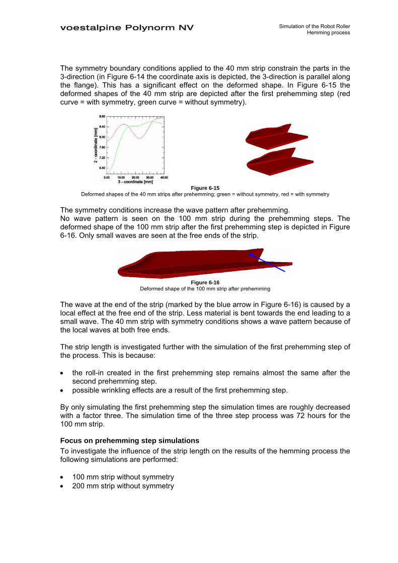
Simulation of the Robot Roller Hemming process
The symmetry boundary conditions applied to the 40 mm strip constrain the parts in the 3-direction (in Figure 6-14 the coordinate axis is depicted, the 3-direction is parallel along the flange). This has a significant effect on the deformed shape. In Figure 6-15 the deformed shapes of the 40 mm strip are depicted after the first prehemming step (red curve = with symmetry, green curve = without symmetry).
Figure 6-15 Deformed shapes of the 40 mm strips after prehemming; green = without symmetry, red = with symmetry
The symmetry conditions increase the wave pattern after prehemming. No wave pattern is seen on the 100 mm strip during the prehemming steps. The deformed shape of the 100 mm strip after the first prehemming step is depicted in Figure 6-16. Only small waves are seen at the free ends of the strip.
Figure 6-16
Deformed shape of the 100 mm strip after prehemming The wave at the end of the strip (marked by the blue arrow in Figure 6-16) is caused by a local effect at the free end of the strip. Less material is bent towards the end leading to a small wave. The 40 mm strip with symmetry conditions shows a wave pattern because of the local waves at both free ends. The strip length is investigated further with the simulation of the first prehemming step of the process. This is because: • the roll-in created in the first prehemming step remains almost the same after the
second prehemming step. • possible wrinkling effects are a result of the first prehemming step. By only simulating the first prehemming step the simulation times are roughly decreased with a factor three. The simulation time of the three step process was 72 hours for the 100 mm strip.
Focus on prehemming step simulations To investigate the influence of the strip length on the results of the hemming process the following simulations are performed: • 100 mm strip without symmetry • 200 mm strip without symmetry

Simulation of the Robot Roller Hemming process
The process settings are the same for all simulations. Both simulations are compared on the roll-in and the deformed shape after prehemming. The 200 mm strip ended at three quarters of the hemming step due to software license problems (the roller has passed 150 mm of the strip). Since the simulation times are extremely long for the 200 mm strip (160 hours till the point where the license problems occurred) the simulation is not performed again and the conclusions are drawn by comparing the results of both simulations till three quarter of the hemming step. Roll-in The roll-in values are average values taken at three points along the hemmed part of the strip (one quarter, half and three quarter of the length). The roll-in values of the prehemming step are given in Table 6-2:
100 mm no symmetry
200 mm no symmetry
Roll-in 0.21 mm 0.20 mm Roll-in variation 0.13 mm 0.13 mm
Table 6-2 Roll-in results
The roll-in values vary the most at the beginning of the strip. After the first 25 mm the roll-in values remain almost constant for both strips. Based on these roll-in results a 100 mm strip with no symmetry conditions can be used in a parameter study. Deformed shape The deformed shapes of the strips are compared with each other by plotting the height of the flange (2-coordinate is the height of the bent flange) along the strip length (3-coordinate is parallel along the strip). These deformed shapes are hemmed for three quarters of the strip length due to the license problems with the 200 mm strip.
Figure 6-17
deformed shape after three-quarters of the last hemming step for the 100 mm and 200 mm strip The deformed shapes are similar for both strips, only the curve of the 200 mm is stretched in the 3-direction. For both strips a small wave at the beginning of the strip is seen. The 100 mm strip showed a wave at the end of the strip. No wave pattern is started from the middle of the 200 mm strip. The 200 mm strip will also give a wave at the end of the 200 mm strip and not at the middle (the position where the wave of the 100 mm strip is seen).

Simulation of the Robot Roller Hemming process
The next section describes the converted model for explicit simulations. These simulations were performed with the goal to decrease the simulation times without losing the results accuracy.
6.2.3. Explicit simulations The simulation times of the implicit models decribed above are relatively long. The prehemming step of the 100 mm strip took over 24 hours to complete. A model can be converted to make it suitable for an explicit analysis. In this analysis scaling options (load and mass scaling) can be applied to speed up the simulation. In this section is investigated if explicit analyses can speed up the simulation without degrading the accuracy of the model. Load- and mass scaling should give the same effects with the same speed-up factor [2]. Since mass scaling is easier to apply (only increasing the density of the material) mass scaling will be applied only. The square root of the mass scaling defines the speed up of the simulation. Started is with a mass scaling of 2500. This should give a speed up of 50 compared to a real time simulation. This amount of scaling gave different results on the deformed shape. Small waves are seen after prehemming along the whole length of the flange (see Figure 6-18; explicit results left, implicit results right). Also the kinetic/internal energy ratio is too high to represent a quasi-static solution.
Figure 6-18 Explicit result, mass scaling 2500 (left) and mass scaling 900 (right) compared to the implicit solution (right)
When the amount of mass scaling is reduced to a factor 900 similar results compared to the implicit solution are found. No wave pattern is seen along the strip length. The wave at the free end in the beginning is increased though, but if this effect is neglected, similar results (roll-in and deformed shape) are seen. The explicit simulation time is approximately similar to the implicit simulation time. In an explicit simulation bulk viscosity damping is applied to prevent high oscillations of the deformable parts. Its goal is to damp the highest frequencies of the deformable parts. The amount of bulk viscosity damping is proportional to the mass density, it has to be increased when no mass scaling is applied to obtain a solution. Otherwise the flange will oscillate at high frequencies resulting in too much element distortion (see Figure 6-19 below). The amount of bulkviscosity damping might influence the results though.
Figure 6-19
Too much element distortion caused by too low bulk viscosity damping Since the simulation times are in the same order as implicit solutions, the implicit solution method will be applied in the parameter study of chapter 7.

Simulation of the Robot Roller Hemming process
6.2.4. Conclusions A 40 mm strip with symmetry boundary conditions can not be used as a representation of a longer strip. The roll-in values are too high, which indicates that the strip is too flexible. By applying the symmetry conditions to the free ends of the 40 mm strip a wave pattern is seen. The local effects of the free ends are increased. It is therefore not possible to represent a longer strip with the symmetry boundary conditions. The roll-in values are not influenced significant by the symmetry boundary conditions. The 100 mm strip will be used in a parameter study to investigate the influence of several different parameters. No symmetry conditions are applied since they only have a local effect. The 100 mm and 200 mm strip with no symmetry conditions gave similar results on roll-in. The explicit simulation method is not efficient for small hemming models. The implicit method is preferred since the simulation times are similar for the 100 mm strip without symmetry. With the implicit method a quasi-static solution is found. In explicit simulations the amount of scaling defines the behaviour of the model. With a mass scaling factor of 900 similar results compared to the implicit model are found. A lot of bulkviscosity damping has to be applied though to obtain a solution. This has an effect on the accuracy level of the simulation. The implicit solution method will therefore be applied for the parameter study in chapter 7 on a 100 mm strip.

Simulation of the Robot Roller Hemming process
7. Parameter study based on a ‘Design of Experiments’ In this chapter the influence of different parameters on the outcome of the robot roller hemming process is given. The goal is to point out parameters with a relatively big influence. These can be analyzed further in future investigations. It is inefficient to investigate the parameters independently from each other. A lot of simulations would be required. The influence of different parameters can be found in fewer simulations by varying different parameters simultaneously in different simulations. One method to do this is by ‘Design of Experiments’ [10]. The parameter study in this chapter is based on Design of Experiments (DOE). In section 7.1 an introduction on DOE is given. The investigated parameters are explained in section 7.2. Their influence on the results is given in section 7.3. An optimization process based on these results is described in section 7.4. This way a design window for desired results like roll-in values can be created.
7.1. Design of experiments A design of experiments is a set of experiments where different factors (parameters) are investigated simultaneously. This way the influence of different factors can be found in less time than would be required if each factor was investigated independently. Also possible interactions between different factors can be identified. There is an interaction between factors when a change of one factor influences the effect of another factor on the results. The principle behind a DOE is illustrated in Figure 7-1 below. In the left table the investigated factors are given (A, B, C and D). These are all two-level factors. The minimum of the factor range is the -1 value (low level) and the maximum is the +1 value (high level). Higher level factors can also be investigated. The middle table represents the design of experiments based on a factorial design. Here all the experiments which are conducted are listed. The number of experiments is dependent on the sort of factorial design (full or fractional). This is described below in section 7.1.1.
Figure 7-1
An example of a Design of Experiments The output of the set of experiments is given in the right table. The response of the investigated model can be divided in two parts: • Main effects (A, B, C and D) • Interactions (AB, AC, AD, BC, BD and CD) A main effect is the effect which one factor has on the model. This is depicted in Figure 7-2. Here both the effect of factor A and B on result 1 are given. Factor A has an increasing effect on result 1. Factor B has a decreasing effect on result 1.

Simulation of the Robot Roller Hemming process
Figure 7-2
Main effects of factor A and factor B Two factors interact with each other when the effect of one factor is dependent upon a second factor. This is depicted in Figure 7-3 below. The effect of factor B is plotted for both values of factor A (this is called A by B). When both lines are parallel to each other no interaction between factor A and B occurs. In Figure 7-3 both lines are not parallel. This means that the value of factor A has an influence on the effect of factor B.
Figure 7-3 Interaction AB, factor A by Factor B
There are different factorial designs available. In the next section only the full and fractional factorial designs are described.
7.1.1. Full or fractional factorial designs In a factorial design the effect of different factors is investigated. There are different designs available, which can be divided in two sorts: full- and fractional factorial designs. In a full factorial experiment, the responses of a model are measured at all combinations of the experimental factor levels. In Figure 7-4 on the next page two examples of full factorial designs are given. Depicted left is a two factor design. Factor A has two levels (-1 and +1) and factor B has three levels (-1 ,0 and +1). The 0-value is the middle value. All the possible factor combinations are investigated. The points in the diagram represent a specific experiment.
Figure 7-4
Two factor (left) and three factor (right) design A three factor design is depicted right. All the factors have two levels. There are eight experiments necessary to investigate all the factors (2f where f represents the number of factors).

Simulation of the Robot Roller Hemming process
To minimize the investigation time some factor combinations can be excluded from the experiments. Factorial designs in which one or more factor level combinations are excluded are called fractional factorial designs. Fractional factorial designs are useful when a large set of factors is investigated. This way the factors which have a big influence are obtained relatively fast. The difference between a full factorial design and fractional factorial design is given in Table 7-1. The number of experiments is given for three two-level factors in: • a full factorial design • a ½ fraction factorial design full
factorial design ½ fraction
factorial design Number of Experiments A B C A B C 1 -1 -1 -1 -1 -1 1 2 1 -1 -1 1 -1 -1 3 -1 1 -1 -1 1 -1 4 1 1 -1 1 1 1 5 -1 -1 1 6 1 -1 1 7 -1 1 1 8 1 1 1
Table 7-1 Full and ½ fraction factorial designs for three two-level factors A, B and C
Also higher fraction factorial designs are available when more factor levels and factor combinations are analyzed. In theory a ¼ fraction of a three factor design results in two experiments. When not all factor level combinations are investigated, some of the effects are lost. When for instance factor A is excluded from the interaction BC, the effect of A includes the effects of BC. Lost effects can not be estimated afterwards with additional experiments. This means that the fraction must be carefully chosen to achieve meaningful results.
Analysis of factorial design results The relation between different variables can be given as a correlation. A correlation coefficient determines if and how two continuous variables are linearly related. The larger the absolute value of the coefficient, the stronger the linear relationship between the variables. An absolute value of one indicates a perfect linear relationship, and a value of zero indicates the absence of a linear relationship. The sign of the coefficient indicates the direction of the relationship. A negative sign means that increasing one factor reduces the result value. The effects of different factors on the results can be statistically significant or non-significant. A statistically significant effect is a response which is not likely to be a result of a chance. The p-value of a correlation determines if the correlation is significantly different from 0. This p-value is compared to a level of significance (α-level). The correlation is different from zero if the p-value is less than or equal to this α-level. A default value is 5 %. This defines the probability of a so called type 1 error. A type 1 error occurs if there is no effect (correlation), while experiments show that there is an effect. The effects of all factors can be compared on relative magnitudes of the effects and the statistical significance of both main and interaction effects. This can be done by a normal probability plot and a pareto chart of the effects (Figure 7-5). The blue line in the normal probability plot (left plot) represents where the points are expected to lie if there are no effects. Significant effects are larger and farther from the line than nonsignificant effects.
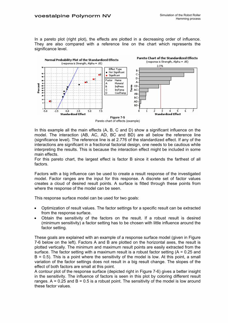
Simulation of the Robot Roller Hemming process
In a pareto plot (right plot), the effects are plotted in a decreasing order of influence. They are also compared with a reference line on the chart which represents the significance level.
Figure 7-5
Pareto chart of effects (example) In this example all the main effects (A, B, C and D) show a significant influence on the model. The interaction (AB, AC, AD, BC and BD) are all below the reference line (significance level). The reference line is at 2.776 of the standardized effect. If any of the interactions are significant in a fractional factorial design, one needs to be cautious while interpreting the results. This is because the interaction effect might be included in some main effects. For this pareto chart, the largest effect is factor B since it extends the farthest of all factors. Factors with a big influence can be used to create a result response of the investigated model. Factor ranges are the input for this response. A discrete set of factor values creates a cloud of desired result points. A surface is fitted through these points from where the response of the model can be seen. This response surface model can be used for two goals: • Optimization of result values. The factor settings for a specific result can be extracted
from the response surface. • Obtain the sensitivity of the factors on the result. If a robust result is desired
(minimum sensitivity) a factor setting has to be chosen with little influence around the factor setting.
These goals are explained with an example of a response surface model (given in Figure 7-6 below on the left). Factors A and B are plotted on the horizontal axes, the result is plotted vertically. The minimum and maximum result points are easily extracted from the surface. The factor setting with a maximum result is a robust factor setting (A = 0.25 and B = 0.5). This is a point where the sensitivity of the model is low. At this point, a small variation of the factor settings does not result in a big result change. The slopes of the effect of both factors are small at this point. A contour plot of the response surface (depicted right in Figure 7-6) gives a better insight in the sensitivity. The influence of factors is seen in this plot by coloring different result ranges. A = 0.25 and B = 0.5 is a robust point. The sensitivity of the model is low around these factor values.

Simulation of the Robot Roller Hemming process
Figure 7-6 Response surface of the model (left) and a contour plot of results versus A and B (right)
The approach of this chapter is to screen different parameters (factors) of the robot roller hemming model in a DOE. The experiments are replaced by simulations. The parameters with the largest influence can be investigated again to create a response surface of the model. This way a process design window can be created for the process engineers and robot programmers.
7.2. Parameters investigated Four parameters are investigated in the first screening of the parameter influence. Only process parameters are investigated. The geometry and the material properties of both the outer and inner part remains the same in all simulations. The parameters investigated in this model are: • TCP – RTP distance • Orientation of the roller • Diameter of the roller • Product overhang The parameters are each described individually in different sections. Also the reason for investigating this parameter is given.
TCP – RTP distance The TCP – RTP distance is defined as the perpendicular distance from the roller tool center point (TCP) to the robot target point (RTP) located at the edge of the hemming bed (Figure 7-7 below).
Figure 7-7
The TCP – RTP distance (schematically) Before each hemming step starts, the roller is moved in the Z-direction of its local axis to bend the flange. In this step the TCP – RTP distance is reached. This distance remains constant during the hemming step.

Simulation of the Robot Roller Hemming process
The TCP-RTP distance is one of the factors which define the amount of deformation during the hemming steps. The minimum value of this parameter is defined with Figure 7-8. First the opening angle of the flange is reduced to 90°. This results in a TCP – RTP distance of 0.761 mm (Figure 7-8, left). This geometrically defined distance is based on no theoretical roll-in of the flange. Assumed is that the outer and inner radius remain the same and no plasticity effects are included.
Figure 7-8
Sketch of the TCP – RTP distance when in theory no roll-in occurs; Based on a roller orientation of 60° (left) TCP – RTP distance is 0.5 mm (right)
When the TCP – RTP distance is 0.5 mm the theoretical roll-in value is 0.3 mm. This value is taken as the low value of the parameter. The high value of this parameter is 1.5 mm. Very little plastic deformation occurs if this distance is increased more (in combination with a roller orientation of 60°) resulting in zero result values. This increases the significance level of the simulation.
Orientation of the roller The orientation of the roller is the angle of the roller with the horizontal (see Figure 7-9 for two orientation angles). The orientation angle of the roller defines in how many steps the product is hemmed. In a standard three step hemming process the orientations are: 60° -> 30° -> 0°. In a two step hemming process they are: 45° -> 0°.
Figure 7-9
Two different orientations of the roller This parameter defines the amount of penetration. For the first prehemming step, the low value is 60° and the high value is 45° (low value on the basis of less deformation).
Diameter of the roller In practice, specific hemming defects caused by robot roller hemming can occur. The flange starts to wrinkle during the prehemming steps. These wrinkles form a wave pattern along the flange of the product. In Figure 7-10 a wave pattern is seen after hemming the flange by roller hemming.

Simulation of the Robot Roller Hemming process
Figure 7-10
A wave pattern on the hemmed flange after hemming During final hemming this wave pattern can be fully flattened out most of the times. But in some cases these wave patterns appear in the end product’s quality after final hemming (depicted in Figure 7-10). On the outer surface of the product the wave pattern can be seen, decreasing the dimensional and surface quality. The diameter of the roller has an effect on the deformation area along the flange. It may therefore have an effect on the forming of wrinkles along the flange. By varying the diameter of the roller its effect on roll-in and wrinkling after prehemming is investigated. The diameter of 20 mm is the low value of this parameter. The high value is 60 mm.
Product overhang When a high volume car is taken out of series production, spare parts production is sometimes performed by robot roller hemming (low volume). In some cases, parts from a former tabletop process have to be hemmed by robot roller hemming. This means that the same roll-in has to be achieved by robot roller hemming as with tabletop hemming. This is most of the times performed with an additional robot roller calibrating step (depicted in Figure 7-11, right). The roller pushes the outer part inwards before the robot roller hemming process starts. In practice the edge of the hemming bed aligns with the dimensions of the finished product (see Figure 7-11, left). Here the required amount of roll-in is depicted. This is equal to the product overhang. In an extreme case a product could have an overhang of 0.8 mm or more.
Figure 7-11
Edge of the hemming bed equals the dimension of the hemmed closure (depicted left); flange bending step (depicted right)
With an overhang, the outer part is less supported by the hemming die. This might have an effect on the result of the hemming process since it gives the flange more freedom during hemming. In this investigation a high value of 0.8 mm and a low value of 0.0 mm (outer part aligns with the edge of the hemming die) are taken. These values are depicted in Figure 7-12. With this parameter is investigated if the additional robot roller calibrating step can be skipped or if the extend of the step can be decreased.

Simulation of the Robot Roller Hemming process
Figure 7-12
Product overhang range: 0.8 mm (high value, left) – 0.0 mm (low value, right) With a product overhang, the robot target point (RTP) does not lie on the hemming bed anymore in the simulations. Otherwise the low value of the TCP – RTP distance is creating too much deformation. The RTP is shifted horizontally with the same amount as the product overhang. The first prehemming step is only investigated first. This is because: • Possible wrinkling effects are a result of a prehemming step. • The difference between continuum shell and solid elements is smaller after
prehemming than final hemming (see Table 5-10 on page 45 for the results of the investigated tabletop model in section 5.2). The similarity between simulations and experiments after prehemming is generally better than the accuracy after final hemming both for solid and shell elements [5]
• Simulating the whole process requires a lot of time (approximately three times more). The results from this first prehemming step are the input of the subsequent steps of the process. The TCP – RTP distance and the orientation of the roller can be varied independently from each other between different hemming steps. Also other roller types can be used for each step (f.i. the final hemming step). One flanging and one prehemming step simulation requires approximately between 24 and 48 hours depending on the amount of deformation. In a full factorial design 16 simulations are needed. For this particular model a full factorial design would require too much time. These parameters are therefore investigated in a ½ fraction factorial design. This means that eight simulations are required to investigate the max and min (-1 and +1) values of the parameters. An additional centerpoint simulation is performed to provide extra accuracy. In a centerpoint simulation middle values of the parameter values are taken. The first goal of this investigation is to obtain parameters which have a big effect on the model. These parameters can be investigated further to create a response surface of the model (section 7.4.1). The second goal is to give a possible method for a future process optimization. This indicates the possibilities of this simulation model.
7.3. Results The first prehemming step is analyzed with a set of simulations. Two sorts of results are analyzed: roll-in and deformed shapes. The priority lies on the roll-in values. Secondarily the forming of wrinkles on the deformed shape after prehemming is investigated. The results are depicted in Table 7-2 on the next page. The parameter values are depicted left. The roll-in and deformed shape results are shown on the right side of the table. Two simulations show wrinkle effects (simulation 4 and 7). These effects are not only a result of a certain combination of TCP - RTP distance and the orientation of the roller. This is because simulation 8 and 3 do not show wrinkling effects with the same TCP –

Simulation of the Robot Roller Hemming process
RTP distances and orientations of the roller as simulation 4 and 7. The wrinkling is therefore also related to the roller diameter. This is more analyzed in section 7.4.2. #: Parameter values: Deformed shape and roll-in results:
TCP – RTP
distance:
Orientation roller:
Diameter roller:
Product overhang:
1 0.5 mm 60° 20 mm 0.0 mm
Roll-in: 0.31 mm
2 1.5 mm 60° 20 mm 0.8 mm
Roll-in: 0.10 mm
3 0.5 mm 45° 20 mm 0.8 mm
Roll-in: 0.39 mm
4 1.5 mm 45° 20 mm 0.0 mm
Roll-in: 0.20 mm
5 0.5 mm 60° 60 mm 0.8 mm
Roll-in: 0.33 mm
6 1.5 mm 60° 60 mm 0.0 mm
Roll-in: 0.09 mm
7 0.5 mm 45° 60 mm 0.0 mm
Roll-in: 0.39 mm
8 1.5 mm 45° 60 mm 0.8 mm
Roll-in: 0.21 mm
9 1.0 mm 37.5° 40 mm 0.4 mm
Roll-in: 0.24 mm Table 7-2
Results of the parameter study of the first prehemming step

Simulation of the Robot Roller Hemming process
The parameters with a big influence on the roll-in are plotted above in the pareto graph of effects. The pareto graph of this design of simulations is plotted in Figure 7-13 below.
Figure 7-13
Pareto chart of effect of the investigated parameters on the roll-in after prehemming Two parameters have a significant influence on the roll-in. Their effects are bigger than the significance level of the results. The TCP – RTP distance has the biggest influence (factor A in Figure 7-13). It has a decreasing effect on the roll-in: when the TCP – RTP distance is increased, the roll-in is reduced. The orientation of the roller (factor B) also has a significant influence on the roll-in. But almost twice as small as the influence of the TCP – RTP distance. It also has a decreasing effect on the roll-in: when the orientation is reduced, the roll-in increases. The effects of A and B are not influenced by a significant interaction. The interaction of parameters A and B is the biggest interaction, but their effect is not judged significant. The effects of the parameters on the wave pattern of the deformed shape can not be plotted in a pareto graph of effects since only two simulations give wavepatterns (#4 and #7). A lot of zero values on for instance wave-amplitude are seen which is resulting in nonsignificant effects. The outer part is not supported less by the die with a product overhang of 0.8 mm. This is depicted in Figure 7-14 for simulation #2. The outer part buckles up during prehemming by the strengthening in the corner of the flange. The contact area with the die starts from a small distance from the edge of the hemming bed. If this contact area was at the edge of the die the outer part would be less constrained.
Figure 7-14
Buckling up of the outer part during prehemming, product has an overhang with the die of 0.8 mm In the next section a roll-in response surface of the model is created for parameters A and B. The forming of wave patterns (seen in simulation #4 and #7) along the flange is also investigated in this section.

Simulation of the Robot Roller Hemming process
7.4. Process optimization The TCP – RTP distance and the orientation θ of the roller have a big effect on the roll-in (factor A and B in Figure 7-13). These two parameters are used to create a roll-in response surface of the model (section 7.4.1). This response surface can be used to create a design window for the process engineers and robot programmers. Furthermore, the forming of wave pattern along the flange is investigated in section 7.4.2 with the goal to reduce these wave patterns.
7.4.1. Optimize on roll-in values A roll-in response surface model is created by varying the two parameters with the biggest effect: the TCP – RTP distance and the orientation θ of the roller. To create a two factor response surface a central composite design is applied. The points of this design are depicted in Figure 7-15. These points represent simulations with different parameter value combinations. The max and min values of two parameters (-1 and +1) are the first points of the response surface. These points are called the ‘cube’ portion of the design depicted left in Figure 7-15. The star points of the design are depicted in the middle figure. The α-values of this design are equal to 1.414. The last point in this design is the centerpoint simulation (0, 0). The complete design is depicted right.
Figure 7-15
Central composite design; Cube portion (left), star portion (middle) and total portion with the centerpoint (right) The max and min values for the TCP – RTP distance and the orientation θ of the roller are the same as used in the DOE simulations and are given in Table 7-3 below. These min max ranges define the response points of the model. The diameter of the roller is 20 mm.
TCP – RTP distance [mm] Orientation θ roller [°] Low value [-1] 0.5 60 High value [+1] 1.5 45
Table 7-3
Response surface The complete response design together with the roll-in results are given in Table 7-4 on the next page. The first four simulations represent the cube portion (high and low values). Simulations 5 to 8 are the star point simulations (with the α-values). The centerpoint simulation is number 9.

Simulation of the Robot Roller Hemming process
Parameter values Roll-in [mm] # TCP – RTP distance [mm] Orientation θ roller [°] 1 0.5 60 0.31 2 1.5 60 0.09 3 0.5 45 0.41 4 1.5 45 0.20 5 0.29289 52.5 0.46 6 1.70711 52.5 0.11 7 1.0 63.1066 0.13 8 1.0 41.8934 0.32 9 1.0 52.5 0.22
Table 7-4 Response surface design together with roll-in results
Through these result points a surface is fit. This gives the roll-in response surface as depicted in Figure 7-16 below left. The horizontal axes represent the parameter values of the TCP – RTP distance and the orientation θ. The roll-in values are given on the vertical axis. The contour plot of this roll-in response is depicted right in Figure 7-16. The dots in this contour plot are the specific parameter combinations used in the simulations. As is expected from the DOE results of section 7.3, the TCP – RTP distance has the largest influence on the roll-in. The slope of the response surface is larger in the TCP – RTP direction than in the orientation direction. This is also seen in the contour plot where there are fewer contour changes in the vertical direction.
Figure 7-16
Roll-in response surface (left) and contour plot of roll-in versus TCP-RTP by orientation (right) This response surface model should be created for every process step for a specific process and with specific goals. Normally the minimum of the surface would be an optimum, to check this optimum a simulation with the following parameters should be run (TCP – RTP distance = 1.70711 mm and orientation = 63.1066°). But for robot roller hemming this exact minimum is not a desired process setting. The minimum is no roll-in which occurs with a very big TCP – RTP distance and a high orientation of the roller. In other words, when no contact between the roller and the outer part occurs. The use of this response surface in practice is explained with two examples based on two production types: • Spare parts production. A specific final roll-in result is desired. In most of the spare parts productions the outer part is developed for a former die or tabletop series production method. When robot roller hemming is the new process for spare parts production, the same amount of roll-in has to be achieved by robot roller hemming. For every prehemming step roll-in response surfaces have to be created where the roll-in values after final hemming have to be equal to the specific roll-in result. Roll-in is to be expected after prehemming and this amount

Simulation of the Robot Roller Hemming process
of roll-in is reduced after final hemming. Example: a final roll-in value of 0.30 mm has to be created. The first prehemming step should create a higher roll-in since the final hemming step creates roll-out. This can be accomplished with a small TCP – RTP distance (≤ 0.5 mm). Different starting points for the next hemming steps are available depending on the orientation of the roller (and the number of prehemming steps). If the orientation is 60° a roll-in value of 0.31 mm is created. This is the starting point for another prehemming step. A response surface of this next step has to be created with new parameter ranges of the TCP – RTP distance and the orientation of the roller. The roll-in result of this second prehemming step should be significantly higher than 0.31 mm, approximately around 0.40 ~ 0.50 mm. This point is the start point for the final hemming step. The TCP – RTP distance and orientation of the roller are known for this step (TCP – RTP distance = 3*part thickness and the orientation of the roller is 0°) so the roll-in value is defined with one additional simulation. This value defines if small adjustments are needed in the previous steps. • New product series production. For series production a stable process setting is desired. This results in a minimal variation in roll-in results. The second goal is to minimize the process time. This means minimizing the amount of hemming steps. The size of the outer part can be compensated later on the roll-in result of the process, so the roll-in is of a less priority. Based on the roll-in response depicted in Figure 7-16, a large TCP – RTP distance has to be chosen. The amount of hemming steps depends on the orientation of the roller. The influence of the orientation of the roller is almost linear (slope remains almost equal). A two step hemming process requires the least process time, so the orientation of the roller should be 45° degrees. Again, this parameter setting combination (f.i. TCP – RTP distance is 1.5 mm and orientation is 45°) is the starting point for the final hemming step. The process settings for the final hemming step are known so by running one simulation the final roll-in values are found. The outer parts have to be compensated on this amount of roll-in so the finished product dimensions are correct. The maximum advantages of this optimization process are obtained when the simulation model is validated with experiments. Only the roll-in values are looked at in this section. The process settings found by this roll-in response surface might not be ideal on other quality areas. Extreme small TCP – RTP distances in the first prehemming step for instance deform the outer radius area which negatively influences the shape of the outer part (curved products like the response result #5 shown in Figure 7-17). Also wave patterns can be formed during prehemming by this particular process setting.
Figure 7-17
Curved product by a extreme small TCP – RTP distance. Response result #5

Simulation of the Robot Roller Hemming process
7.4.2. Wave pattern reduction Two simulations of the first parameter screening of the DOE gave wave patterns after the prehemming step. Simulation #4 and simulation #7. The deformed shapes are plotted again in Figure 7-18.
Figure 7-18
A wave pattern on the hemmed flange after prehemming; Simulation #4 (left) and simulation #7 (right) The forming mechanism of the robot roller hemming process is analyzed with the goal to understand these wrinkling effects after prehemming. The factors which determine the forming mechanism in these simulations are described first. Main factors of the forming mechanism The forming mechanism of roller hemming is influenced by two different factors: • A line in the 1-2-plane of the global axis which bends the flange (blue line in Figure
7-19). The position and orientation of this line is defined by the TCP – RTP distance and the orientation of the roller. In Figure 7-19 two process settings are depicted. Depicted left: TCP – RTP distance = 0.5 mm, orientation of the roller θ = 60°. The process setting of the right figure is: TCP – RTP distance = 1.0 mm, orientation of the roller θ = 45°.
Figure 7-19
Main forming line (blue) Left: TCP – RTP = 0.5 mm, Orientation θ = 60°; Right: TCP – RTP = 1.0 mm, Orientation θ = 45°
• The roller diameter. The roller diameters of 20 and 60 mm gave wave patterns after
prehemming in the DOE simulations. The flange opening angle after the hemming step and the amount of roll-in is defined by the line in the 1-2-plane (blue line in Figure 7-19): • Simulation #1 and #5: 0.31 mm and 0.33 mm roll-in. Opening angle is 60°. • Simulation #2 and #6: 0.10 mm and 0.09 mm roll-in. Opening angle is 60°. • Simulation #3 and #7: 0.39 mm roll-in for both. Opening angle is 45°. • Simulation #4 and #8: 0.20 mm and 0.21 mm roll-in. Opening angle is 45°. After the DOE investigation, simulation number 4 showed a wave pattern along the flange after prehemming. Simulation number 8 had the same position and orientation of the forming line. Only a bigger roller diameter (60 mm in stead of 20 mm) was used and the product overhang was 0.8 mm in stead of 0.0 mm. Since the product overhang does not change the amount of support by the die (see Figure 7-14), the change in roller

Simulation of the Robot Roller Hemming process
diameter influences the forming of waves. The results of both these simulations are analyzed further below.
Simulation results The simulations of a 20 mm and 60 mm roller are compared with each other with the same process settings. The position and orientation of the forming line depicted in Figure 7-19 is the same for both simulations and based on: TCP – RTP distance = 1.5 mm and the orientation of the roller θ = 45°. The deformed shape and roll-in values are given in Table 7-5. Diameter Roller: 20 mm Diameter Roller: 60 mm
Deformed shape
Roll-in [mm] 0.20 0.21
Table 7-5 TCP – RTP distance = 1.5 mm and Orientation roller θ = 45°
One of the conclusions of chapter 6 was that the symmetry boundary conditions applied to the edges of the parts increase the amplitude of waves. Symmetry conditions constrain the parts in the global 3-direction. The stresses and strains in the material are therefore first analyzed in the global 3-direction. The plate material stresses can be divided in a 1- and 2- direction in the plane of the plate, and a 3-direction in the thickness of the plate (depicted in Figure 7-20 below). The 2-direction is parallel to the strip and equals the 3-direction of the global coordinate axis.
Figure 7-20
Plate material coordinate axis
Analysis of stress during the process The stresses in the 2-direction are plotted in Figure 7-21 on the next page for both simulations.

Simulation of the Robot Roller Hemming process
Diameter Roller: 20 mm Diameter Roller: 60 mm S22
[MPa]
Figure 7-21 Stresses in the 2-direction; 2-direction of the plate material is parallel to the strip
More peak S22 stresses are seen in the top of the flange for the bigger roller. These S22 stresses in the material change during the process. Different stress areas are plotted in Figure 7-22 for the smaller roller. The area in front of the roller is depicted right, in the middle figure the area at the roller is depicted. The area behind the roller is depicted left. As can be seen in the figures, the stresses differ from the inside and outside area of the flange. At all areas their states are opposite (tensile – compression). And during the process the stress state alternates between tensile and compression.
Behind the roller
Inside flange - Outside flange
At the roller
Inside flange - Outside flange
In front of the roller
Inside flange - Outside flange Figure 7-22
Stresses in the 2-direction of the plate material for the smaller roller The S22 stress distribution is different for both rollers across the height of the flange (see Figure 7-21, differences in contours between both rollers). The peak S22 stress areas are more distributed over the height of the flange for the smaller roller. Furthermore, the peak values are also higher for the smaller roller. At approximately a quarter of the flange height the S22 stress state of the smaller roller changes from approximately 358 MPa to -316 MPa. For the bigger roller this S22 stress varies from 150 MPa to -150 MPa. The reason for this is explained in Figure 7-23. At all flange heights the smaller roller will bent the flange more. The original flange is represented by the dotted line. The S22 stress peaks are higher for the smaller roller. This is seen by the tangent line of the roller at the crossing with the original flange, angle α > β. This results in higher S22 stress variations than the bigger roller.

Simulation of the Robot Roller Hemming process
Figure 7-23
The flange (dotted line) is bent extremer around a smaller roller. The tangent line of the roller at the flange has a larger angle with the smaller roller
Analysis of plastic strains during the process The higher S22 stress values of the smaller roller creates more strain in the 2-direction of the plate (PE22). The PE22 strain plots are plotted for both rollers in Figure 7-24.
Diameter Roller: 20 mm Diameter Roller: 60 mm PE22
Figure 7-24 Strains in the 2-direction; 2-direction of the plate material is parallel to the strip;
The outside flange (depicted at the bottom) shows a PE22 strain area in front of the roller, the inside flange a PE22 strain area at the roller. The peak values are higher at the top of the flange for the smaller roller. There is also more PE22 strain located lower in the flange. The strains are now monitored at different heights of the flange around the middle of the strip. The monitored points are plotted in Figure 7-25.
Figure 7-25
Monitored points in the flange

Simulation of the Robot Roller Hemming process
The PE22 strain variation at the monitored points is plotted for both rollers in Table 7-6. At time 7.4 ~ 7.5 the roller passes the monitored points.
Diameter Roller: 20 mm Diameter Roller: 60 mm
PE22 strain
Top of the flange
Half of the flange height
Quarter of the flange height
Table 7-6
PE22 strains at different flange heights; Inside area (red), outside area (green) From the plastic strain history plots, the following is observed: • At all three monitored points over the height of the flange, the strain history patterns
are similar, for both rollers. • Differences are seen in the peak values:
- At the top of the flange the peak values are almost equal for both rollers. - At half and quarter height of the flange, the peak values for the smaller rollers are much higher than for the roller with the larger diameter.

Simulation of the Robot Roller Hemming process
Analysis of resulting plastic strains after the process The resulting PE22 strains are plotted below in Figure 7-26.
Diameter Roller: 20 mm Diameter Roller: 60 mm PE22
Figure 7-26
Resulting strains in the 2-direction after the prehemming step For the bigger roller almost no resulting PE22 strains are seen in the top of the flange. This on the contrary with the smaller roller which shows local PE22 strains in the top. These PE22 strains vary from tensile to compressed areas.
Summary stress-strain analysis The smaller roller shows a wave pattern in the flange after the process, whereas the larger roller does not. Based on the previous observation and analysis, the following conclusions are drawn: • When the roller passes the flange, each point in the flange undergoes subsequently
a forth and back bending deformation. • The diameter of the roller determines the peak value of the occurring bending stress;
the smaller the diameter, the higher the peak stress value. • The diameter of the roller also determines the size of the stress and strain
distribution; the larger diameter shows only a local stress and strain concentration at the top of the flange (point contact). The smaller roller shows a stress and strain concentration over the full height of the flange (line contact).
• Because the smaller roller shows a resulting wave pattern in the flange after the process, it is concluded that this is determined by the following two conditions: 1. the value of the peak bending stress. 2. the stress distribution over the height of the flange (point contact versus line
contact). Therefore, it is concluded that when the peak bending stress is high enough and also distributed over the height of the flange (line contact), a wave pattern results in the flange after the process. This wave pattern is showed by a changing tensile and compressive plastic strain in the flange, as shown in the left in Figure 7-26. However, it cannot be explained yet why a changing tensile and compressive plastic strain distribution occurs in the flange. This is investigated further in the next section.
Analysis of forming mechanism The theory behind the forming mechanism is explained with Figure 7-27. From top to bottom the prehemming is depicted at different time steps. In Figure 7-27 the static equilibrium situations along the flange are depicted for these times. The deformed sections A/F are now analyzed. At time 1 (Figure 7-27a), it is assumed that section A

Simulation of the Robot Roller Hemming process
and C are plastically deformed for the first time. This is shown in the figure by the yellow color of A and C. All other sections are elastically deformed (green). At time 2, the roller moves to section B. The static equilibrium situation in this case is depicted in Figure 7-27b. Because of the yellow parts are work hardened, and the force is equal to the force in situation a, the material of section B will only elastically deform.
Time 1: a
Time 2: b
Time 3: c
Time 4: d
Time 5: e
Figure 7-27
Equilibrium states at different times of the prehemming step When the roller moves to location C, the situation as depicted in Figure 7-27c occurs. Because of the material before and after the roller has not work hardened yet, these areas are deformed plastically. The material under the roller will undergo plastic deformation for the second time, when the force is large enough. Now the roller moves to section D. Again looking at the force equilibrium and taking into account the work hardening history, the situation in Figure 7-27d occurs. Section C was twice plastically deformed and is thus the most strengthened area. Sections D and E need to compensate this in an equilibrium state. This results in the plastic deformation of section E. Finally when the roller reached section E, the equilibrium situation depicted in Figure 7-27e applies. Section D has been work hardened. Sections E and F will both plastic deform to fulfill the equilibrium. This situation equals the situation of Figure 7-27c and this process will therefore be continued till the end of the prehemming step. The resulting PE22 strain of this process is depicted in Figure 7-28 on the next page. The PE22 strains at both side of all the sections are depicted with + (longer) and – (shorter). The resulting + and – PE22 strains depend on the shape of the section when it undergoes plastic deformation (when plastic deformation occurs for the second time, the state is changed).

Simulation of the Robot Roller Hemming process
Figure 7-28
Deformation of different section (A/F) during prehemming The resulting PE22 strains at the inner and outer side of the flange are now alternating (the resulting states depicted at time 5 in Figure 7-28). It is concluded that the forming of wave patterns occurs under two conditions by robot roller hemming: • The roller force must be great enough to stress the areas under the roller in such a
way that plastic deformation occurs twice on a section (Section C and E, Figure 7-28) • A line contact between the roller and the flange has to be achieved. This way the
PE22 strains are distributed over the height of the flange and the resulting PE22 strains are significant.
With the larger roller the equilibrium situation of Figure 7-27c does not occur. Section C will only undergo elastic deformation resulting in the equilibrium situation depicted in Figure 7-29.
Figure 7-29
Equilibrium state for a larger roller (left); C is not deformed plastically for the second time (right) When the TCP – RTP distance is decreased more, these wave patterns also occur with a larger roller. This is seen in simulations 7 and 3 of the DOE of section 7.3 the TCP – RTP distance is decreased to 0.5 mm for both rollers. Now the bigger diameter roller gives a wave pattern because a line contact is achieved and the roller force is now high enough. For the smaller roller no wave pattern is seen. The results are depicted in Table 7-7.

Simulation of the Robot Roller Hemming process
Diameter Roller: 20 mm Diameter Roller: 60 mm
Deformed shape
Roll-in [mm] 0.39 0.39 Table 7-7
TCP – RTP distance = 0.5 mm and Orientation roller θ = 45° The resulting PE22 strains after prehemming are plotted below for both rollers.
Diameter Roller: 20 mm Diameter Roller: 60 mm PE22
Table 7-8 Resulting strains in the 2-direction after the prehemming step
In this case the outer radius area is stressed by the smaller roller. This area is already strengthened by the flanging process and the flange is therefore pushed more inwards than with the larger roller (depicted in Figure 7-30). A point contact between the roller and the outer radius area is achieved. Therefore the flange buckles more up than with the larger roller (compare Figure 7-30 to the deformed shape in Table 7-2 for simulation #7 with the larger roller).
Figure 7-30
Deformed shape during prehemming of simulation #3: 20 mm roller, TCP – RTP = 0.5 mm and orientation roller = 45°
Simulation of the Robot Roller Hemming process
7.4.3. Conclusions Optimization on roll-in results is possible with a DOE. A roll-in response surface must be created for every prehemming step. The points on the response surface of the prehemming step are possible starting points for the next hemming step. When this step is a prehemming step another response surface has to be created. When this step is a final hemming step, the result after final hemming is the total roll-in. This optimization method can be used for different goals. For spare parts production, optimization on a specific roll-in result is desired. After final hemming the roll-in value must be equal to this specific roll-in result. After prehemming a starting point for a next prehemming step or a final hemming step has to be chosen. This starting point must have created more roll-in because this amount of roll-in is reduced in the final hemming step. For new parts production, a stable process is desired. The optimal process point has little variation of roll-in around that area. This is seen at large TCP – RTP distances. The smallest process time is also desired because of the higher production volume compared to spare parts production. Since the orientation of the roller almost shows a linear influence on the roll-in variation, a two step hemming process is the optimum result. So the orientation of the roller is 45°. The position and orientation of the forming line of Figure 7-19 determines the amount of roll-in. The position and orientation is defined by the TCP – RTP distance and the orientation of the roller. Simulations of the DOE with the same process settings but other roller diameters gave the same roll-in results. The diameter of the roller has an influence on the forming of waves along the flange. These wave patterns occur if: • The roller force must be great enough to stress the areas under the roller in such a
way that plastic deformation occurs twice under the roller. This is achieved with a certain TCP – RTP distance and orientation of the roller.
• A line contact between the roller and the flange has to be achieved. This way the PE22 strains are distributed over the height of the flange and the resulting PE22 strains are significant.
A line contact is achieved at higher TCP – RTP distances with a smaller roller than with a larger roller. The larger roller shows only a local stress and strain concentration at the top of the flange (point contact). The smaller roller shows a stress and strain concentration over the full height of the flange (line contact). The tendency towards wrinkling is therefore reduced by: • A larger roller. No plastic deformation occurs for the second time. • Changing the position and orientation of the forming line of Figure 7-19. When the
TCP – RTP distance is increased (roller is further away from the hemming bed), the roller force is reduced. The equilibrium is achieved by the elastic deformation of the area in front of the roller and behind the roller.

Simulation of the Robot Roller Hemming process
8. Conclusions and Recommendations
8.1. Conclusions • Die and tabletop hemming processes with flat-surface parts are well simulated with a
2D simulation model. A qualitative comparison on roll-in is possible. • When a quantitative comparison on roll-in is desired, specific material properties and
models have to be defined. Differences are seen with different material hardening models (differences of 35 % in roll-in are seen between Nadai and Voce hardening models).
• The implicit solution method out performs the explicit method in simulation times for the relative small models in this report (small in terms of number of elements). For the 2D simulations of chapter 5 and the 3D tabletop strip model the simulation times are significant smaller for the implicit method. The simulation times of the 100 mm strip of the robot roller hemming model are in the same order for both the prehemming and final hemming step.
• The conventional shell, continuum shell and 3D solid elements (all linear reduced) can all be applied in robot roller hemming simulations of the prehemming step. This is tested with a small tabletop model whereby roll-in was seen after prehemming. The roll-in deviation between these elements is small (5%).
• The continuum shell element is the most efficient element for the large 3D robot roller hemming simulations. With one element over the thickness of the parts, the simulation times are the lowest with acceptable accuracy.
• A 100 mm strip length with no symmetry boundary conditions applied on the edges is sufficient to simulate wide flat-surface parts. The roll-in results have to be measured in the middle part of the strip. Otherwise local effects at the free ends are disturbing the accuracy.
• The results after prehemming are dependind on: the TCP – RTP distance, the orientation of the roller and the diameter of the roller. The TCP – RTP distance and the orientation of the roller determine the amount of roll-in. The diameter of the roller determines the deformed shape locally during the prehemming and has therefore an influence on the forming of wave patterns along the flange.

Simulation of the Robot Roller Hemming process
8.2. Recommendations • Before this simulation model can be used in further investigations validation tests
have to be performed on flat-surface test strips. The whole robot roller hemming process has to be performed including the flanging step. The following things have to be investigated correctly: the material properties (real stress/strain data and possible anisotropy) and the influence of friction between the components in contact. When these factors are correctly stored in the simulation model, the influence of the element-type can be investigated again. The difference in roll-in between shell and solid elements was smaller after prehemming then after final hemming for the 3D tabletop model of the small strip. These differences are probably also seen after a total robot roller hemming simulation. With validation tests of this simulation it becomes clear which element is the most accurate for robot roller hemming simulations.
• The friction has to be added between the roller and outer part, and a revolting roller (which can rotate freely around its revolution axis) has to be modeled in simulations to see if this has an effect on roll-in results with constant diameter rollers. With other roller types and lead angles friction between the roller and outer part plays a more important roll because of the slip areas between the roller and the flange.
• The material properties for materials under cyclic loading have to be investigated properly. Since the forming of waves occurs with plasticity changes due to cyclic loading, the influence of a Bauschinger effect is significant.
• After the validation process a design of experiments can create response surfaces
for each hemming step of a specific product. The material and geometry of the product are a constant input to the model. In practice, some hemming processes require different rollers. A smaller roller might be needed in the final hemming step to prevent collisions with the inner part or downholder on highly curved products. The following factors have to be used as an input for a DOE of a certain product (with a certain geometry and material): TCP – RTP distance, orientation θ of the roller, the diameter/type of roller and the lead angle β of the roller. The result output is a five dimensional (four factors and one result) roll-in response and a five dimensional wave-amplitude response of the first prehemming step. From these responses an optimal parameter setting must be chosen for the second hemming step (another prehemming step or final hemming step) because the result of the first prehemming step influences the next step(s).
• When complete parts are to be simulated (large number of elements) the explicit solution method will outperform the implicit method in terms of simulation times. The implicit solution of a certain section of that part is still desired though as a reference for the explicit solution. This way the amount of scaling (mass or load) for the explicit method has to be defined accurately. The result of a stamping simulation can be mapped from an Autoform® stamping simulation to hemming simulations in Abaqus® to increase the quantity of the results. Autoform® is simulation software dedicated to stamping simulations and is therefore more efficient than Abaqus® for stamping simulations.
• Springback of hemmed parts should be investigated. This way defects like warpage and wave effects after the final hemming step can be predicted. The springback should be performed with the implicit method since springback can be regarded as a static problem without loading and contact. Explicit simulation results can be imported to an implicit model for this purpose.
• With extreme small TCP – RTP values (< 0.5 mm) the mesh density of the simulation model is too coarse in the outer radius area. Adaptive meshing is desired which is possible with solid elements. This problem should not occur with conventional shell

Simulation of the Robot Roller Hemming process
elements which represent the midsurface of the parts. The unstable behaviour of these elements during the lasts phase of the final hemming step should therefore be investigated more.
• This simulation model should be used in problem areas of the assembly department. Small geometries can be simulated when the local effects are neglected of the free ends.

Simulation of the Robot Roller Hemming process
List of References [1] Jonkers, B., Hemming Basics, an overview of all the different hemming
technologies and their variants. Polynorm Automotive, Bunschoten, 2005. p. 22-26.
[2] Abaqus® Analysis users manual, version 6.6. 2005. [3] Meijers, E., Ontwerpen van dunne plaat producten en de Eindige Elementen
Methode. Vereniging FME-CWM, Zoetermeer, 2004. [4] Huetink, J., Meinders, V.T., Plasticity. Universiteit Twente, Enschede, 2006. [5] Sigvant, M., The hemming process, a Numerical and Experimental Study.
Chalmers University of Technology, Göteborg, Sweden 2003. [6] Le Maoût, N., Numerical simulation of flat-surface roll hemming: Influence of
geometry and material models. Université de Bretagne-Sud, France 2006. [7] Bördeln of Aluminium. Polynorm Grau, Swäbisch Gmund, 1996. [8] Haar ter, R., Friction in Sheet Metal Forming, the influence of (local) contact
conditions and deformation. Universiteit Twente, Enschede, 1996. p. iv. [9] Li K.P.; W.P. Carden, R.H. Wagoner. Simulation of Springback. I.J. Mech. Sc.
Vol. 44. p. 103 – 122, 2002. [10] Trygg, J., Wold, S., Introduction to statistical experimental design, a.k.a. design of
experiments (DoE). Umeå University, Sweden, 2004. [11] Laar van, J., based on private communications with Jan van Laar, robot
programmer. Bunschoten, 2006.

Simulation of the Robot Roller Hemming process
List of Appendi
Appendix A: Assignment
Appendix B: Implicit method
Appendix C: Explicit method
Appendix D: Contact interactions of both solution methods
Appendix E: Simulation Results

Simulation of the Robot Roller Hemming process
Appendix A: Assignment
Simulation of the Robot Roller Hemming Process Introduction Polynorm is a leading Tier 1 supplier to the automotive industry, specialised in project management, design, engineering, development and production of class - A body panels and components made from steel, aluminium, plastic and hybrid materials. One of Polynorm’s objectives is to expand it’s assembly capacities and capabilities. A technology to assemble closures (doors, hoods, trunklids) is the so-called robot roller hemming technology, which is integrated in flexible robot cells. Robot Roller Hemming To hem closures, several technologies are available on the market, such as die hemming and table top hemming. Robot roller hemming has been introduced at the market in the late nineties and has been applied by Polynorm since the year 2000. In principle the robot roller hemming process consists of a roller, which is manipulated by a robot along a programmed path. This roller “bends” the flange in three steps (90 60 30 0) to a into closed hem and creates therewith a assembled closure. The closure is supported by an anvil, which also serves as the reference for the programmed robot path.
Problem Description Currently too little know-how is available with regard to the robot roller hemming process itself. Achieving and maintaining the required quality (dimensional, surface) is therefore an “trial-and-error” outcome. To enable a more stable product and process quality as well as a shorter time-to-market, finite element simulations of the robot roller hemming process would be helpful to define and optimise the process. Assignment Final targets for Polynorm are to obtain process setting guidelines to: • Control dimensional and surface quality • Reduce process time (fewer process steps)
To reach these final targets with the aid of FEA Simulations, the following intermediate targets are set: • Build a three dimensional FEA model, which can describe the Robot Roller Hemming forming
process; • Analyse the simulation results to increase insight in the process;

Simulation of the Robot Roller Hemming process
• Perform a parameter study: analyse the influence of different parameters, investigate which are important for the final product quality and process time, and finally optimize these parameters.
Approach 1. Study which parameters has to be identified in the models, for:
• Material: start with simple elastic-plastic isotropic model • Product geometry (starting and final) • Roller: geometry, position, orientation and loading (force/displacement) • Anvil and Down Holder (boundary conditions, constraints)
2. Choose one reference situation of parameter setting and start with a 2D-model. Expected results from the 2D model are:
• Analysis of difference between continuum and shell elements • Prediction of roll-in (shrinkage of product geometry due to hemming process)
3. With experience from the 2D-model, build a 3D-model (Implicit and/or Explicit). Expected results from the 3D model are:
• Analysis of the simulation results in terms of stress, strain and deformation • Economically feasibility of 3D model with respect to simulation time and accuracy
4. Analyse the influence of the different parameters identified in step 1. on final product dimension (roll-in), surface quality (wrinkling) and process time;
5. Optimize these parameters and obtain process design & process parameter guidelines; 6. Validate the simulation results with practical experiments. The Robot Roller Hemming Simulations should be executed with the ABAQUS FEA Package. The Assignment is preferred to be conducted within the Polynorm Group at the Bunschoten premises (see also www.polynorm.com). An assignment payment is included. For more information Please contact: • Dr.ir. Timo T. Meinders, Mechanics of Forming Processes, University of Twente,
[email protected], phone: 053 - 489 4360 • Ir. Laurens F. van der Sande, Corporate Engineering, Polynorm N.V., [email protected],
phone: 033 - 298 9932

Simulation of the Robot Roller Hemming process
Appendix B: Implicit method of Abaqus® In Abaqus® two solver methods are available:
• Direct lineair equation solver: Uses a sparse, direct, Gauss elimination method. In nonlinear analysis ABAQUS/Standard uses the Newton method or a variant of it, such as the Riks method, within which it is necessary to solve a set of linear equations at each iteration. Problems suited for this solver method: Spoked wheel. Not suited: Blocky structures.
• Iterative lineair equation solver: Uses a domain decomposition method. Need a symmetric stiffness matrix and a single load case. Suited for blocky structures.
Newton method: Differences between external forces P and internal nodal forces I are checked after each iteration. The internal loads acting on each node are produced by the stresses within the element.
For the body to be in equilibrium, the net force acting at every node must be zero. That results in: P – I = 0. The nonlinear load-displacement curve for a structure is:
The nonlinear response of a structure to a small load increment ΔP is:
The configuration at u0 is used to find the structure’s tangent stiffness K0. With ΔP the displacement correction ca is determined whereby the structure is updated to ua. The internal forces are then calculated and equilibrium is checked with the following equation: P – Ia = Ra where Ra is the force residual of the iteration.

Simulation of the Robot Roller Hemming process
If Ra is zero at every degree of freedom in the model, point a in the above figure would lie on the load-deflection curve and the structure would be in equilibrium. In a nonlinear problem Ra will never be exactly zero, so it is compared to a tolerance value. If Ra is less than this force residual tolerance at all nodes, ABAQUS/Standard accepts the solution as being in equilibrium. By default, this tolerance value is set to 0.5% of an average force in the structure, averaged over time. If Ra is less than the current tolerance value, P and Ia are considered to be in equilibrium and ua is a valid equilibrium configuration for the structure under the applied load. However, before ABAQUS/Standard accepts the solution, it also checks that the last displacement correction, ca, is small relative to the total incremental displacement, Δu = ua – u0. If ca is greater than a fraction (1% by default) of the incremental displacement, ABAQUS/Standard performs another iteration. Both convergence checks must be satisfied before a solution is said to have converged for that time increment. If the solution from an iteration is not converged, another iteration is performed to try to bring the internal and external forces into balance. First, the new tangent stiffness Ka is calculated for the structure based on the updated configuration, ua. This stiffness, together with the residual Ra, determines another displacement correction, cb, that brings the system closer to equilibrium:
The new force residual Rb is calculated. Again two checks for convergence, tolerance factor on Rb and cb is compared with Δub. For each iteration in a nonlinear analysis the model's stiffness matrix is formed and a system of equations is solved.

Simulation of the Robot Roller Hemming process
Appendix C: Explicit method of Abaqus® An explicit dynamic analysis allows for the definition of very general contact conditions and can be used to perform quasi-static analyses with complicated contact conditions. It can therefore be used in analyses where implicit solvers may have problems with convergence. The explicit dynamics procedure performs a large number of small time increments. An explicit central-difference time integration rule is used, each increment is relatively inexpensive (compared to the direct-integration dynamic analysis procedure used in implicit procedures) because there is no solution for a set of simultaneous equations. The explicit central-difference operator satisfies the dynamic equilibrium equations (F = m.a) at the beginning of the increment, t. The accelerations calculated at time t are used to advance the velocity solution to time t + Δt/2 and the displacement solution to time t + Δt. The explicit dynamics analysis procedure is based upon the implementation of an explicit integration rule together with the use of diagonal (‘lumped’) element mass matrices. The equations of motion for the body are integrated using the explicit central-difference integration rule:
Nii
Ni
Ni
Ni
iiNi
Ni
utuu
utt
uu
)()1()()1(
)()()1(
)()(
21
21
21
2
+++
+
−+
Δ+=
Δ+Δ+=
&
&&&&
Where ui is a degree of freedom (a displacement or rotational component) and the subscript i refers to the increment in an explicit dynamics step. The central-difference integration operator is explicit in the sense that the kinematic state is advanced using known values of N
iu )( 21−
& and
Niu )(&& from the previous increment.
The explicit integration rule is quite simple but by itself does not provide the computational efficiency associated with the explicit dynamics procedure. The key to the computational efficiency of the explicit procedure is the use of diagonal element mass matrices because the accelerations at the beginning of the increment are computed by:
( ) ( )Ji
Ji
NJNi IPMu )()(
1)( −=
−&&
Where MNJ is the mass matrix, PJ the applied load vector and IJ is the internal force vector. A lumped mass matrix is used because its inverse is simple to compute and because the vector multiplication of the mass inverse by the inertial force requires only n operations, where n is the number of degrees of freedom in the model. The explicit procedure requires no iterations and no tangent stiffness matrix. The internal force vector, IJ, is assembled from contributions from the individual elements such that a global stiffness matrix need not be formed. The explicit integration scheme in ABAQUS/Explicit requires nodal mass or inertia to exist at all activated degrees of freedom unless constraints are applied using boundary conditions. A nonzero nodal mass must exist unless all activated translational degrees of freedom are constrained and nonzero rotary inertia must exist unless all activated rotational degrees of freedom are constrained. Nodes that are part of a rigid body do not require mass, but the entire rigid body must possess mass and inertia unless constraints are used.
The explicit procedure integrates through time by using many small time increments. The central-difference operator is conditionally stable, and the stability limit for the operator (with no damping) is given in terms of the highest frequency of the system as:

Simulation of the Robot Roller Hemming process
max
2ω
≤Δt
An approximation to the stability limit is often written as the smallest transit time of a dilatational wave across any of the elements in the mesh:
dcL
t min≈Δ
where Lmin is the smallest element dimension in the mesh and cd is the dilatational wave speed in terms of 0λ and 0μ , defined below.
This estimate for Δt is only approximate and in most cases is not a conservative (safe) estimate. In general, the actual stable time increment chosen by ABAQUS/Explicit will be less than this estimate by a factor between 21 and 1 in a two-dimensional model and between 31 and 1 in a three-dimensional model. The time increment chosen also accounts for any stiffness behavior in a model associated with penalty contact.
The current dilatational wave speed, cd, is determined in ABAQUS/Explicit by calculating the effective hypo-elastic material moduli from the material's constitutive response. Effective Lamé's constants, λ̂ and μ̂2ˆ =G , are determined in the following manner. Define Δp as the increment
in the mean stress, ΔS as the increment in the deviatoric stress, volεΔ as the increment of
volumetric strain, and εΔ as the deviatoric strain increment. We assume a hypo-elastic stress-strain rule of the form:
( )εμ
εμλΔ=Δ
Δ+=Δˆ2
ˆ2ˆ3Sp vol
The effective moduli can then be computed with:
( )μμλ
εεεμ
εμλ
ˆ4ˆ331ˆ2ˆ::ˆ2
ˆ2ˆ3ˆ3
+=+
ΔΔΔΔ
=
ΔΔ
=+=
K
S
pKvol
These effective moduli represent the element stiffness and determine the current dilatational wave speed in the element as:
ρμλ ˆ2ˆ +
=dc
where ρ is the density of the material.

Simulation of the Robot Roller Hemming process
In an isotropic, elastic material the effective Lamé's constants can be defined in terms of Young's modulus, E, and Poisson's ratio, ν , by:
( )( )
( )νμμ
νννλλ
+==
−+==
12ˆ
211ˆ
0
0
E
E
The time increment used in an analysis must be smaller than the stability limit of the central-difference operator. Failure to use a small enough time increment will result in an unstable solution. When the solution becomes unstable, the time history response of solution variables such as displacements will usually oscillate with increasing amplitudes. The total energy balance will also change significantly. If the model contains only one material type, the initial time increment is directly proportional to the size of the smallest element in the mesh. If the mesh contains uniform size elements but contains multiple material descriptions, the element with the highest wave speed will determine the initial time increment. The use of small increments (dictated by the stability limit) is advantageous because it allows the solution to proceed without iterations and without requiring tangent stiffness matrices to be formed. It also simplifies the treatment of contact.
The explicit dynamics procedure is suited for analyzing high-speed dynamic events, but many of the advantages of the explicit procedure also apply to the analysis of slower (quasi-static) processes. An example is sheet metal forming, where contact dominates the solution and local instabilities may form due to wrinkling of the sheet.
Bulkviscosity damping In an explicit analysis, bulk viscosity introduces damping associated with volumetric straining. Its purpose is to improve the modelling of high-speed dynamic events. Two forms of bulk viscosity are available, linear and quadratic. The bulk viscosity parameters b1 (linear coefficient) and b2 (quadratic coefficient) define the amount of damping. Linear bulk viscosity is found in all elements and is introduced to damp ‘ringing’ in the highest element frequency. This damping is sometimes referred to as truncation frequency damping. It generates a bulk viscosity pressure that is linear in the volumetric strain rate: voldbv Lcbp ερ &∈= 11 . The second form of bulk viscosity pressure is quadratic in the
volumetric strain rate (only found in solid continuum elements): ( ) .222 volbv Lbp ερ &∈= Quadratic
bulk viscosity is applied only if the volumetric strain rate is compressive. The quadratic bulk viscosity pressure will smear a shock front across several elements and is introduced to prevent elements from collapsing under extremely high velocity gradients. Consider a simple one-element problem in which the nodes on one side of the element are fixed and the nodes on the other side have an initial velocity in the direction of the fixed nodes. If the initial velocity is equal to the dilatational wave speed of the material, without the quadratic bulk viscosity, the element would collapse to zero volume in one time increment (because the stable time increment size is exactly the transit time of a dilatational wave across the element). The quadratic bulk viscosity pressure will introduce a resisting pressure that will prevent the element from collapsing. The linear bulk viscosity coefficient b1 is by default 0.06. The quadratic bulk viscosity coefficient b2 is by default 1.2. Load and mass scaling In an explicit analysis load and mass scaling can be applied to speed up the analysis. Load scaling is applied by increasing the tool speeds. Mass scaling is applied by increasing the density of the model. For quasi-static problems a maximum allowable scaling is to be checked with the kinetic and internal energy ratio. The kinetic energy must be a small fraction (≤ 5%) of the internal energy.

Simulation of the Robot Roller Hemming process
First the influence of the speed-up factor on both load- and mass scaling is determined. The results from the load- and mass scaling simulations are given at the end. The accelerations at the beginning of the increment are computed by:
( ) ( )Ji
Ji
NJNi IPMu )()(
1)( −=
−&&
Where MNJ is the mass matrix, PJ the applied load vector and IJ is the internal force vector. For a simulation model with no scaling methods used this gives thus (simplified):
a = F/m (1)
Load scaling applied with a factor f:
When load scaling is applied to the model the steptimes are decreased (for instance resulting in higher tool speeds). Influence of the factor f on the simulation model:
Toolspeeds increased with factor f ⇒ Accelerations increased with a factor f Accelerations increased with a factor f ⇒ Loads (external and internal) increased with a factor f)
( ) [ ]( )Ji
Ji
NJNi IPfMuf )()(
1)( −⋅=⋅
−&&
mFam
Ffaf /=⇒⋅
=⋅ (2)
Mass scaling applied with a factor f2:
By artificially increasing the material density, ρ, by a factor of f2 decreases the wave speed by a factor of f and increases the stable time increment by a factor of f. The result is the same speed-up of the simulation as with load scaling factor f. For a linear elastic material with poisson ratio equal to zero the wave speed is defined as:
ρEc =
The influence of factor f2 on the simulation model is:
Mass increased with a factor f2 ⇒ Loads increased with a factor f2 Mass increased with factor f2 ⇒ Wave speed decreased with factor f
Wave speed decreased with factor f ⇒ Stable time increment increased with factor f
)(dc
Lt ∈=Δ
The loads are applied with the same speed ⇒ Accelerations are the same
( ) ( )[ ]Ji
Ji
NJNi IPfMfu )()(
212)( −=
−&&
mF
MfFfa == 2
2
(3)

Simulation of the Robot Roller Hemming process
Equations (1), (2) and (3) are equal so the same speed-up factor has the same influence on the results. Equation of State material In explicit simulations with low scaling a warning that the ratio of the deformation speed to the wave speed is greater to 0.3 is given. Generally when this ratio is too high, it is an indication that the purely mechanical material constitutive relationship is no longer valid and that a thermo-mechanical equation of state material is required. The equation for conservation of energy equates the increase in internal energy per unit mass, Em, to the rate at which work is being done by the stresses and the rate at which heat is being added. In the absence of heat conduction the energy equation can be written as:
( ) QSt
ppt
Ebv
m && ρερρ
ρ ++∂∂
−=∂∂
:1
Where p is the pressure stress defined as positive in compression, pbv is the pressure stress due to the bulkviscosity (explained later), S is the deviatoric stress tensor, ε& is the deviatoric part of strain rate, and Q& is the heat rate per unit mass. The equation of state is assumed for the pressure as a function of the current density ρ and the internal energy per unit mass, Em:
),( mEfp ρ= This defines all the equilibrium states that can exist in a material. The internal energy can be eliminated from the above equation to obtain a p versus V relationship (V = current volume) or
equivalently, a p versus ρ1 relationship that is unique to the material described by the equation
of state model. This unique relationship is called the Hugoniot curve and is the locus of p-V states achievable behind a shock.
The Hugoniot pressure, pH, is a function of density only and can be defined, in general, from fitting experimental data. A Mie-Grüneisen equation of state is linear in energy. The most common form is ( ),HmH EEpp −Γ=− ρ where EH
is the Hugoniot specific energy (per unit mass) and are functions of density only. Γ is the Grüneisen ratio defined
as ρρ0
0Γ=Γ . The Hugoniot energy, EH, is related to
the Hugoniot pressure by Hugoniot curve

Simulation of the Robot Roller Hemming process
02ρηH
HpE = where ρρη /1 0−= is the nominal volumetric compressive strain. Elimination of
Γ and EH from the above equations yields .2
1 000
mH Epp ρη
Γ+⎟⎠⎞
⎜⎝⎛ Γ−= The equation of state
and the energy equation represent coupled equations for pressure and internal energy. Linear equations of state can always be written in the form ,mgEfp += where f and g are functions of density only and depend on the particular equation of state model.
A common fit to the Hugoniot data is given by ( )
,1 2
200
ηηρ
sc
pH−
= where c0 and s define the linear
relationship between the linear shock velocity, Us, and the particle velocity, Up, as follows: .0 ps sUcU += With the above assumptions the linear Us – Up Hugoniot form is written as
( ),
21
1 000
2
200
mEsc
p ρη
ηηρ
Γ+⎟⎠⎞
⎜⎝⎛ Γ−
−= where 2
00cρ is equivalent to the elastic bulk modulus at
small nominal strains. There is a limiting compression given by the denominator of this form of the equation of state
10
lim −=
ssρ
ρ . At this limit there is a tensile minimum, thereafter negative sound speeds are
calculated for the material. The initial state of the material is determined by the initial values of specific energy, Em, and pressure stress, p. If no initial conditions are specified the material is at its reference state: Em = 0, p = 0, .0ρρ = To prevent heavily element distortion a thermo-mechanical equation of state can be defined by specifying the reference density 0ρ and the variables c0, s and .0Γ

Simulation of the Robot Roller Hemming process
Appendix D: Contact interactions in Abaqus® For both the implicit and explicit method in Abaqus® two contact discretization methods are available: node-to-surface and surface-to-surface discretization. Also two tracking approaches are available: the small and finite sliding approach. The implicit method uses a pure master slave method, the explicit method uses a weighted master slave method (kinematic enforcement method). This means that one contact area is first the master surface and after that the slave surface. The calculated contact pressures (of both surfaces) are then averaged. Node-to-surface discretization: Contact interactions are established such that each ‘slave’ node on one side of a contact interface interacts with a point of projection on the master-surface on the opposite side of the contact interface. One single slave node and o a group of nearby master nodes are considered. Surface-to-surface discretization: The goal of the surface-to-surface discretization is to optimize stress accuracy, both surfaces in contact are considered. Contact conditions are enforced in an average sense over the slave-surface, some penetration may occur. The surface-to-surface discretization uses more constraints and can therefore increase solution costs. Surface-to-surface is costly by: • simulations where a large part of the model is in contact • if the master surface is more refined than the slave surface • different layers of slave- and master surfaces (f.i. inner part/ outer part contact) In general the node-to-surface approach is less costly in simulations. The two tracking approaches define the relative motion of the contact surfaces. The finite sliding approach is the most general tracking approach which allows for separation, sliding and rotation of surfaces. The small sliding approach is a special approach for contact with little sliding of surfaces. It is based on a linearized approximation of the master surface.

Simulation of the Robot Roller Hemming process
Appendix E: Simulation model and result details Polynorm Grau case (original results): This study deals with the hemming of test parts of aluminum with the die hemming process. Due to its limited formability compared to hemming steels another hem shape is needed. The aluminum alloys deployed in 1996 (date of the study) were not suitable for a flat hem shape. By using a rope hem the outer radius is increased which thereby reduces the tension in that area (see figures below for a rope hem). This way defects like cracks on the outer radius surface or shape defects (warpage, recoil) are prevented.
A1: A rope hem (left) and a flat hem (right)
Section results:
A2: Section results with different tool parameters after prehemming (above left) and final hemming
Original roll-in graphs:
A3: Original roll-in results: Above left: R45 variation Above right: R2 variation
Below left: S variation 2D simulation model development

Simulation of the Robot Roller Hemming process
The mesh of the 2D model is given below and is refined near the area where the hem develops.
A4: Mesh on the outer and inner part
The number of elements over the thickness is investigated. Simulations with 4, 6, 8 and 10 elements over the thickness are compared. Simulations with 4 elements over the thickness show a sharper stress and strain contour compared to the other simulations. Little differences in contours are seen in the simulations with 6, 8 and 10 elements over the thickness. Also the maximum and minimum equivalent plastic strain values are within 5 % of each other. The roll-in values are plotted below:
0
0.05
0.1
0.15
0.2
0.25
0.3
0.35
2 4 6 8 10
Number of elements over the thickness
roll-
in [m
m]
Final hemming Prehemming
A5: Influence of the number of elements over the thickness on the roll-in
A deviation in roll-in is seen with the model with eight elements over the thickness. This deviation is a result of the mesh density on the outer radius edge. See figures below for the outer radius edge of the simulation with 6 elements over the thickness and 8 elements over the thickness. The amount of roll-in is measured with the help of the node positioned on the edge of the hem (encircled in red). With the simulation with six elements over the thickness this node sticks more out of the hem than with the simulation with eight elements. This is the reason for the difference in roll-in (0.170 mm against 0.176 mm). This deviation is thus not related to the change in number of elements over the thickness. To lessen this effect of the discretization an average of roll-in will be taken over the three outer nodes. Based on these results, six elements over the thickness is sufficient for the 2D simulations.

Simulation of the Robot Roller Hemming process
A6:
6 elements over the thickness 8 elements over the thickness Load scaling applied to the 2D model: A guideline for the upperbound of the load scaling is equal to 10% of the wave speed of the material. For aluminium with a poisson ratio equal to 0.3 the wave speed is approximately 6000 m/s. Punch speed is then equal to 60 m/s.
As can be seen in the next figure, the punch speed is too high and produces an unrealistic result. Therefore the upperbound of the load scaling is too high.
A7: Punch speed too high The punch speed based on the real situation is 100 mm/s. By applying a scaling factor of 50 the punch speed is equal to 5000 mm/s. A check with the energies (figures below) shows that this load scaling produces a quasi-static solution. For a quasi-static analysis the kinetic energy must be a small fraction of the internal energy (here it is 2.2 %).
Between the different load scaling simulations a big difference in the amount of roll-in is seen. Load scaling factor 30 produces the same results as the implicit method so these values are taken in the parameter value study. At low amount of scaling element distortions are seen. The distorted elements are gone when the amount of scaling is increased above a certain factor. To prevent heavily element distortion a thermo-mechanical equation of state (see appendix 2) can be defined by specifying the reference density 0ρ and the variables c0, s and .0Γ Since these material constants are not yet available and their value is not easy to define this is left undone.

Simulation of the Robot Roller Hemming process
Material hardening model (Nadai versus Voce) The stress/strain curves of the DC04 deep drawing steel are depicted below. Nadai hardening assumes hardening at high strain levels. The Voce model neglects hardening at high strain levels.
0
50
100
150
200
250
300
350
400
450
500
0 0.05 0.1 0.15 0.2 0.25 0.3 0.35 0.4 0.45
Strain [%]
Stre
ss [M
Pa]
Nadai Voce
A8: Stress/strain curves of DC04 based on two hardening models
The influence of the hardening model is tested with the following model parameters: R45 = 15 mm, R2 = 2.5 mm and S = 1.2 mm. The results are given below:
Two different hardening models roll-in [mm] Plastic strain [%] Mises stress [MPa] Nadai 0,42 68,4 336Voce 0,31 81,4 255
A9: Influence of different hardening models on the roll-in The difference in roll-in is approximately 35 % so the effect is high. A good hardening model investigation must therefore be performed for different materials when a quantitative solution is needed. Simulation results of the tabletop model of section 5.2 (element-type comparison): The incompatible solid element behaves too stiff in the simulation. Roll-in is seen during the final hemming step, which is unlikely in practice. The deformed shape during the flanging step is also unrealistic:
A10: The flanging step for the simulation with an incompatible 3D solid
The conventional shell gave a lot of problems during the simple tabletop simulation. During the final hemming step unstable buckling of the top of the flange occurred. The simulation also requires a lot of alterations to make it suitable for an implicit analysis. The thickness definition of a conventional shell can give problems in contact simulations. In implicit analyses the thickness between two deformable bodies is defined by default. But the thickness between an analytical rigid tool and a deformable part is only taking into account with surface-to-surface contact with both sliding approaches and node-to-surface contact with small sliding. The small sliding approach is not the right approximation for the changing contacts in hemming simulations. And the surface-to-surface discretization with the conventional shell element is not suited for hemming

Simulation of the Robot Roller Hemming process
simulations where a large part of the simulation involves contact. This is because of the extremely large simulation times. So a switch to the more general node-to-surface discretization in combination with the finite-sliding approach is needed. A negative contact interference is defined to take the thickness into account (a contact interference is normally a tolerance zone which defines a possible penetration distance of a slave node through a master surface). This way the tools contact the shell from a distance equal to half the thickness of a shell (see figure below on the right). This way the thickness of the shell is taken into account.
A11: Default node-to-surface contact which does not account for shell thickness [left]; node-to-surface contact with a negative contact interference of half the shell thickness [right]
3D robot roller hemming model The mesh of the 3D model (continuum shell element, no stacking) is given below and is refined near the area where the hem develops. Element size in the flange area of the outerpanel:
(0.2 mm*0.4 mm*0.7mm)
A12: Mesh on the outer and inner part

Simulation of the Robot Roller Hemming process
Simultation results of section 7.4.2. The PE22 strain of simulation number 4 is plotted below:
A13: PE22 strains at different positions