SIMULATION OF THE DYNAMICALLY

COUPLED KC-135 TANKER AND REFUELING BOOM

THESIS

Jeremy J. Smith, Captain, USAF AFIT/GAE/ENY/07-M21 DEPARTMENT OF THE AIR FORCE

AIR UNIVERSITY

AIR FORCE INSTITUTE OF TECHNOLOGY

Wright-Patterson Air Force Base, Ohio

APPROVED FOR PUBLIC RELEASE; DISTRIBUTION UNLIMITED

The views expressed in this thesis are those of the author and do not reflect the official

policy or position of the United States Air Force, Department of Defense, or the United

States Government.

AFIT/GAE/ENY/07-M21

SIMULATION OF THE DYNAMICALLY COUPLED KC-135 TANKER AND REFUELING BOOM

THESIS

Presented to the Faculty

Department of Aeronautics and Astronautics

Graduate School of Engineering and Management

Air Force Institute of Technology

Air University

Air Education and Training Command

In Partial Fulfillment of the Requirements for the

Degree of Master of Science in Aeronautical Engineering

Jeremy J. Smith, BSAE

Captain, USAF

March 2007

APPROVED FOR PUBLIC RELEASE; DISTRIBUTION UNLIMITED.

AFIT/GAE/ENY/07-M21

SIMULATION OF THE DYNAMICALLY COUPLED KC-135 TANKER AND REFUELING BOOM

Jeremy J. Smith, BSAE Captain, USAF

Approved: ____________________________________ Dr. Donald L. Kunz (Chairman) date ____________________________________ Major Eric Swenson (Member) date ____________________________________ Major Paul Blue (Member) date

AFIT/GAE/ENY/07M-21

Abstract

Future Air Force requirements for the use of unmanned aircraft will require

Automated Aerial Refueling (AAR). Current AAR research requires a precision model

to simulate the refueling process of a KC-135 tanker and a UAV. There are existing high

fidelity models of the tanker aircraft, refueling boom and proposed receiver aircraft.

However, none of the models are coupled. Since boom orientation and motion is known

to change the trim of the tanker aircraft, which in turn influences all other aspects of the

refueling process, a new model is needed.

The new model was created by integrating an existing KC-135 tanker and

refueling boom model. The tanker boom equations of motion were coupled using joint

coordinates and the velocity transformation. Assessment of the new model investigated

boom and tanker motion in comparison with other established models. Ultimately,

behavior of the new model was validated by a comparison of simulation results to flight

test data.

The research culminated with the successful validation of the new model. Boom

and tanker behavior of the new model matched that of both the established tanker and

boom models as well as the flight test data. Even though the KC-135 has been flying for

nearly 50 years, this is the first model that captures the dynamic interactions of the

aircraft and its aerial refueling boom.

iv

ACKNOWLEDGEMENTS

I would like to express my extreme gratitude to my thesis advisor, Dr. Donald Kunz for

his guidance throughout the course of this research. In addition to the faculty here at

AFIT, I would like to thank my elemetary and high school teachers for giving me the

foundation that has enabled me to reach this point. Finally, and most importantly, I

would like to thank my family back home, who have been and always will be the best

teachers anyone could ask for.

v

Table of Contents

Page Abstract ...................................................................................................................... iv Acknowledgements ......................................................................................................v Table of Contents ....................................................................................................... vi List of Figures ........................................................................................................... viii List of Tables ...............................................................................................................x List of Symbols .......................................................................................................... xi I. Introduction ............................................................................................................1 Background.............................................................................................................1 System Description .................................................................................................2 Existing Models ......................................................................................................6 Current AAR Research ...........................................................................................8 Problem Statement ..................................................................................................9 Research Objectives................................................................................................9 II. Methodology ........................................................................................................11 Overview..............................................................................................................11 Coupled Equations of Motion..............................................................................11 The AFRL KC-135 Model...................................................................................19 Implementing the Coupled Equations of Motion in the AFRL Tanker Model ...22 III. Data Analysis .......................................................................................................30 Overview..............................................................................................................30 Test Scenario Setup .............................................................................................32 Boom Motion with Tanker in Unaccelerated Straight and Level Flight .............37 The Effect of Coupling the Tanker and Boom.....................................................36 Tanker Effects on Boom Motion with Boom Control Inputs ..............................40 Boom Effects on Tanker Motion with Boom Control Inputs ..............................43 Comparison to Flight Test Data...........................................................................46 IV. Conclusions and Recommendations ...................................................................53 Conclusions..........................................................................................................53 Page

vi

Suggestions for Further Study .............................................................................54 Appendix A. Modified Simulink Blocks ....................................................................56 Appendix B. Flight Test Data Test Cases...................................................................61 Appendix C. Embedded Matlab Functions.................................................................73 Bibliography ..............................................................................................................107 Vita.............................................................................................................................109

vii

List of Figures

Figure Page 1. USAF KC-135 Stratotanker with Flying Boom in the Stowed Position (3)...........3 2. KC-135 with Refueling Boom Pitched Down (11:2) .............................................4 3. Boom Fork (12).......................................................................................................4 4. NACA 65-012 Airfoil Showing Ruddevator Chord (13) .......................................5 5. Refueling Boom Ruddevator Layout (1) ................................................................5 6. Rigid Bodies Connected by Mechanical Joints ....................................................13 7. Origin of Coordinate Frames Used to Derive the Uncoupled Equations of Motion (14)...............................................................................................................................14 8. Major Systems of the AFRL Tanker Model .........................................................20 9. The Vehicle Model System, Associated Subsystems, and Their Inputs and Outputs......................................................................................................................................20 10. Subsystems of Rigid Body Motion Including Inputs and Outputs .......................22 11. Ruddevator Coordinate Frames (1).......................................................................27 12. Boom Pitch Response to a Six Degree Symmetric Ruddevator Deflection .........33 13. Boom Yaw and Pitch Response to a Six Degree Asymmetric Ruddevator Deflection......................................................................................................................................36 14. Tanker Pitch Angle Comparison from the Coupled and AFRL Model ................38 15. Boom Pitch Angle Comparison: Coupled and Steady, Level Flight Constrained38 16. Comparison of Boom Pitch Response to a Six Degree Symmetric Ruddevator Deflection.....................................................................................................................40 17. Comparison of Boom Pitch and Yaw Response to a Six Degree Asymmetric Ruddevator Deflection.................................................................................................42

viii

Page 18. Tanker Pitch Response to a Ten Degree Symmetric Ruddevator Deflection.......43 19. Tanker Pitch, Roll and Yaw Response to a Ten Degree Asymmetric Ruddevator Deflection.....................................................................................................................45 20. Boom Response to a Symmetric Ruddevator Control Schedule: Flight Test Data –vs- Simulation ..............................................................................................................50 21. Boom Response to an Asymmetric Ruddevator Control Schedule: Flight Test Data –vs- Simulation ..............................................................................................................52

ix

List of Tables

Table Page 1. Mechanical Joints .................................................................................................12 2. List of Embedded Matlab Functions and their Purpose........................................24 3. Nominal States for and Assumed Trimmed Tanker/Boom System .....................32

x

List of Symbols a......................acceleration vector AX,AY,AZ..........tanker velocity components B .....................velocity transformation matrix C .....................direction cosine matrix F .....................force vector, or block matrix for a floating joint I ......................3x3 Identity matrix I ......................Inertia matrix for a component M ....................moment vector, or Mach number m.....................mass n......................unit vector defining principal motion axis P .....................block matrix for a prismatic joint P,Q,R..............tanker roll, pitch, and yaw rates Q.....................generalized force r ......................position vector U.....................block matrix for a universal joint uE ....................extended length of the boom extension VX,VY,VZ..........tanker velocity components Greek symbols η .....................joint velocity or acceleration vector �B...................tanker pitch angle B

�F...................fixed boom pitch angle �B...................tanker roll angle B

�B...................tanker yaw angle B

�F...................fixed boom yaw angle � ....................angular velocity vector Superscripts and subscripts B .....................tanker E .....................boom extension F .....................fixed boom I ......................inertial reference frame S......................overall system

xi

Reference Frames B .....................tanker reference frame E .....................boom extension reference frame F .....................fixed boom reference frame I ......................inertial reference frame W ruddevator reference frame Operators (·) time derivative (~) skew symmetric matrix defined such that TA A= −

xii

SIMULATION OF THE DYNAMICALLY COUPLED KC-135 TANKER AND

REFULEING BOOM

I. Introduction

Background

Unmanned Aerial Vehicles (UAVs) are becoming more and more of an important

component of the modern battlespace. The Predator and Global Hawk are predominantly

intelligence gathering aircraft designed to loiter above and turn their vast array of sensors

down on the battlefield for extended periods of time. Since Predator’s inception in 1995,

it has been equipped with hellfire missiles in order to interdict time sensitive targets on

the ground. A greatly upgraded, hunter-killer version of the Predator, the MQ-9 Reaper,

is now in System Design and Development with a full rate production decision expected

in 2009. The advancements include a 3000lb payload capacity to include the capability

of delivering 500lb Joint Direct Attack Munitions.

When this current generation of UAVs deploys to a theater of operations, they

must be broken down at their home station, boxed up, flown to their new base,

reassembled and then test flown. This disassembly-reassembly process must be

accomplished before the aircraft can actually take part in a mission. This is a somewhat

satisfactory arrangement given the mission and relative complexity of the aircraft

involved. However, expanded roles and aircraft are already being developed for the

second generation UAVs. The Unmanned Combat Aerial Vehicle (UCAV) technology

demonstrator was originally intended as a small, relatively short range aircraft for use in

Suppression of Enemy Air Defense (SEAD) missions. The aircraft has since been

expanded to a vehicle about the size of an F-35 with same variety of missions including

1

formation flight, multi aircraft attack and aerial refueling. Refueling a UAV in flight

introduces issues not experienced during manned refueling operations. In order to

address these issues and to train personnel involved in the refueling process, advanced,

high-fidelity models and simulations are necessary.

Currently, high-fidelity models of the KC-135 tanker, the refueling boom, and the

UAVs exist separately, but no existing single system models the dynamic interactions

among them. In order for second generation UAVs to deploy from stateside home

stations to overseas theaters without going through the disassembly-reassembly process,

UAVs must be capable of Automated Aerial Refueling (AAR). A high fidelity model

integrating the behavior of the tanker, boom, and UAV must be developed in order to

facilitate this. This thesis will serve as the first step in generating this fully integrated

model for AAR simulations by developing a coupled, high fidelity model of the KC-135

tanker and refueling boom.

System Description

The USAF KC-135 family of tanker aircraft are derivatives of the Boeing 707,

America’s first transport plane powered by turbojet engines (see Figure 1). Originally

designed and built in the 1950’s, more than 500 KC-135’s remain in the USAF inventory

today. The aircraft is 136.25’ long, has a wingspan of 130.83’ and is capable of carrying

a transferable fuel load of 200,000 lbs. Fuel is transferred from tanker to receiver via a

flying boom.

During refueling, the receiver aircraft basically flies in formation with the tanker

and a boom operator flies the boom into contact with the receiver’s receptacle. The

2

boom operator lies prone in a control station facing aft in the bulbous section of the aft

fuselage directly below USAF aircraft identifying marker.

Figure 1. USAF KC-135 Stratotanker with Flying Boom in the Stowed Position (3).

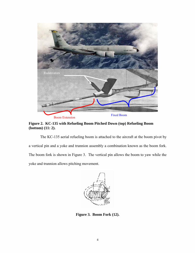
The flying boom itself consists of two distinct pieces. The fixed boom is the

portion that can be seen in Figure 1 and consists of 27.75’ long tube-like fairing with an

elliptical cross section. The fixed boom travels aft from the boom attachment point, past

the fairing that houses the boom’s control surfaces and ends at the tip as seen above in

Figure 1. The boom extension can be seen in Figure 2. It is a 27’ foot long cylinder with

a fuel transfer nozzle at the tip. While in the stowed position, the boom extension is

retracted completely inside the fixed boom. The extension can extend out of the fixed

boom to a maximum extension position of 20 feet outside the fixed boom.

3

Fixed Boom

Boom Extension

Ruddevators

Figure 2. KC-135 with Refueling Boom Pitched Down (top) Refueling Boom (bottom) (11: 2).

The KC-135 aerial refueling boom is attached to the aircraft at the boom pivot by

a vertical pin and a yoke and trunnion assembly a combination known as the boom fork.

The boom fork is shown in Figure 3. The vertical pin allows the boom to yaw while the

yoke and trunnion allows pitching movement.

Figure 3. Boom Fork (12).

4

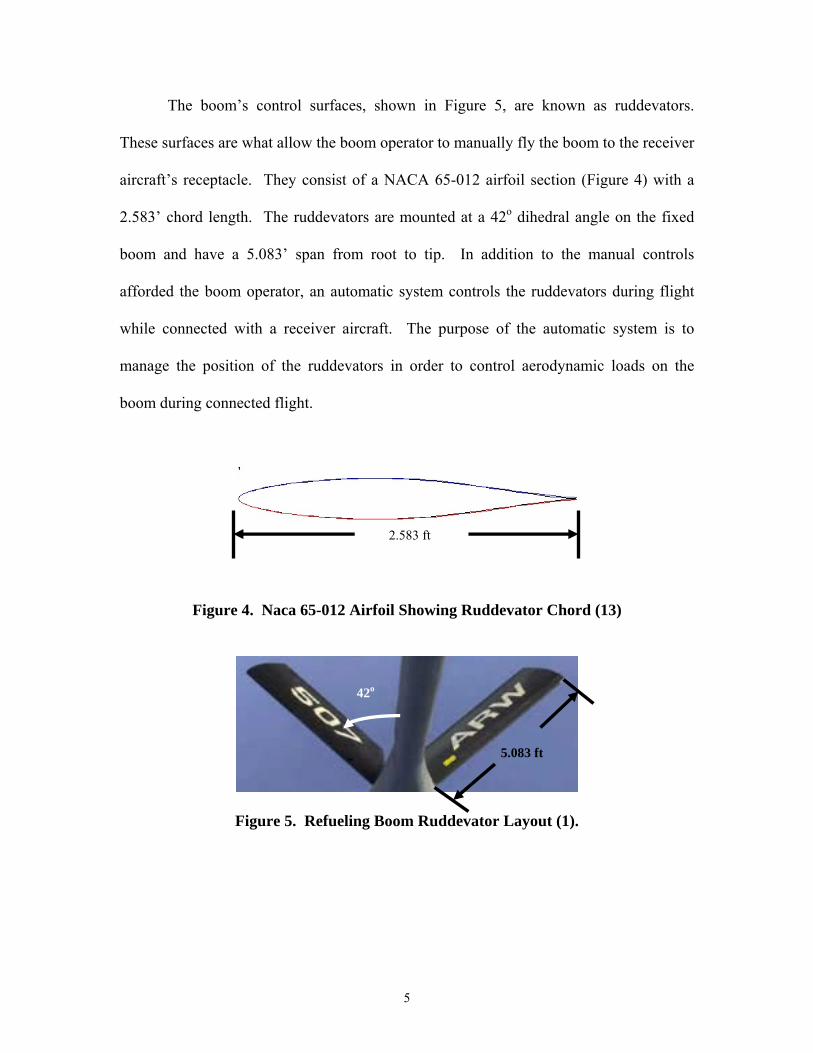
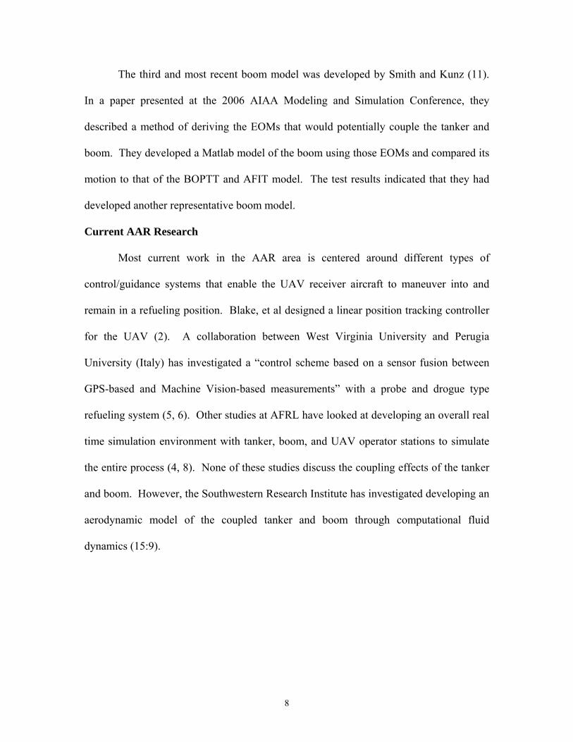
The boom’s control surfaces, shown in Figure 5, are known as ruddevators.

These surfaces are what allow the boom operator to manually fly the boom to the receiver

aircraft’s receptacle. They consist of a NACA 65-012 airfoil section (Figure 4) with a

2.583’ chord length. The ruddevators are mounted at a 42o dihedral angle on the fixed

boom and have a 5.083’ span from root to tip. In addition to the manual controls

afforded the boom operator, an automatic system controls the ruddevators during flight

while connected with a receiver aircraft. The purpose of the automatic system is to

manage the position of the ruddevators in order to control aerodynamic loads on the

boom during connected flight.

2.583 ft

Figure 4. Naca 65-012 Airfoil Showing Ruddevator Chord (13)

Figure 5. Refueling Boom Ruddevator Layout (1).

5.083 ft

42o

5

Existing Models

Currently, there are high fidelity models of both the KC-135 and its refueling

boom, but in no existing model are the dynamic interactions between the tanker and

boom taken into account.

The high fidelity KC-135 tanker model was developed for the Air Force Research

Laboratory (AFRL). The model was written in Simulink and aircraft states, such as

mass, orientation, speed, and altitude, can be initialized from two separate Matlab script

files. The model has the ability to operate on autopilot mode for both straight and level

and typical race-track type refueling patterns or to take manually commanded pilot

inputs. The boom pivot location is attached and tracked, though again, there are no

interactions between the tanker and boom.

The model basically consists of a few major systems broken down into numerous

sub and other minor systems. The major systems include the autopilot, control system

and the actual vehicle model. The Vehicle Model system contains all the aerodynamic

and moment of inertia calculations that are fed into the tanker’s equations of motion

(EOMs).

The tanker EOMs were developed with the typical aircraft coordinate system

(origin located at the tanker’s mass center, the x-axis going out the nose, the y-axis

pointing to right and z axis pointing down). The EOMs are written in the following

form:

[ ]

[ ] [ ]{ }{ }

{ }{ } [ ][ ]{ }

[ ] 00B Fvm

M II ω ωω⎡ ⎤ ⎧ ⎫⎧ ⎫⎪ ⎪ ⎪ ⎪=⎨ ⎬ ⎨ ⎬⎢ ⎥ −⎪ ⎪ ⎪ ⎪⎩ ⎭ ⎩⎣ ⎦

I

⎭ (1)

6

where the far left hand term is the 6x6 mass/inertia matrix, the second term on the left

hand side is the 6x1 vector of linear and angular accelerations, and the right hand side is a

6x1 vector of aerodynamic and gravitational forces and moments acting on the tanker.

This is the matrix-vector version of Newton’s Second Law of Motion, F = ma or M =

Iω .

To solve Equation 1, the AFRL model calculates the force/moment vector on the

right hand side from the aircraft states. The EOMs are solved for the acceleration vector

by multiplying both sides of Equation 1 by the inverse of the mass/inertia matrix. The

acceleration vector is then integrated twice to find velocity and position vectors for the

tanker. Prior to the second integration, the angular rates must be transformed to aircraft

attitude rates.

In this research, three models of the boom will be discussed. The first is the

Boom Operator Part Task Trainer (BOPTT). This model is used in the training of boom

operators and has been used in tandem with AFRL’s tanker model to perform AAR

simulations even though they do not model the dynamic interactions between the tanker

and boom. Development of the EOMs for this model treated the boom as a stand alone

rigid body attached to the tanker at the boom fork. The boom fork was assumed to

translate through the air as though on an imaginary rigid rail. The boom itself was

allowed to go through its normal motion, but neither model was affected by the other.

The second boom model was developed at the Air Force Institute of Technology

(AFIT) by Campbell in 1989. Again, EOM development considered the boom as a

standalone rigid body. This model was developed to research the possibility of

expanding the boom’s refueling envelope (7:1).

7

The third and most recent boom model was developed by Smith and Kunz (11).

In a paper presented at the 2006 AIAA Modeling and Simulation Conference, they

described a method of deriving the EOMs that would potentially couple the tanker and

boom. They developed a Matlab model of the boom using those EOMs and compared its

motion to that of the BOPTT and AFIT model. The test results indicated that they had

developed another representative boom model.

Current AAR Research

Most current work in the AAR area is centered around different types of

control/guidance systems that enable the UAV receiver aircraft to maneuver into and

remain in a refueling position. Blake, et al designed a linear position tracking controller

for the UAV (2). A collaboration between West Virginia University and Perugia

University (Italy) has investigated a “control scheme based on a sensor fusion between

GPS-based and Machine Vision-based measurements” with a probe and drogue type

refueling system (5, 6). Other studies at AFRL have looked at developing an overall real

time simulation environment with tanker, boom, and UAV operator stations to simulate

the entire process (4, 8). None of these studies discuss the coupling effects of the tanker

and boom. However, the Southwestern Research Institute has investigated developing an

aerodynamic model of the coupled tanker and boom through computational fluid

dynamics (15:9).

8

Problem Statement

While the AFRL tanker model and the three boom models are all valid training

tools and offer insight into the behavior of the tanker and boom, no existing model can

describe the behavior of the tanker and boom as a single system. For manned refueling

missions, this is satisfactory because each person in the loop (tanker pilot, boom operator,

receiver pilot) can make any necessary adjustments to ensure the refueling event is a

success. This will not be the case during AAR because one of the decision makers, the

receiver pilot, has been taken out of the loop. In order to accurately predict behaviors of

the tanker boom system, a new model must be developed that couples the dynamic

interactions between the KC-135 tanker and its refueling boom.

Research objectives:

The objective of this research is to develop and validate a dynamically coupled

model of the KC-135 and its refueling boom that has the potential to be an effective

research tool. AFRL’s KC-135 Simulink model will serve as the baseline program to be

modified. In order to leave the majority of this highly reliable model untouched, most

modifications to this program will be made to the Vehicle Model system. Every effort

will be made to ensure that the original inputs and outputs will remain as is, though some

things will inevitably have to change. The EOMs and boom model developed by Kunz

and Smith will serve as tools to help modify the AFRL tanker model and in turn develop

the first dynamically coupled model of the KC-135 tanker and its refueling boom.

9

Validation of the new model will initially be accomplished by examining its

simulation results against those obtained from AFRL’s KC-135 model and the

Kunz/Smith boom model. Evaluation of the model will include investigating motion of

the boom and tanker as separate entities, and then as a coupled system.

Tanker response to the attached boom and commanded changes in boom motion

will be examined, as will changes in boom motion due to it being dynamically attached to

the tanker. There should be some visible effects from the coupling of the tanker and

boom, but these changes should be rather small in nature. Final validation of the new

model will come from comparing the coupled model’s simulation results with existing

flight test data. The data includes tanker and boom responses to commanded changes in

boom position.

10

II Methodology

Overview

This chapter will discuss Kunz and Smith’s development of the coupled EOMs

for the tanker and boom, the AFRL Simulink model and its operation, and finally the

method in which the two models were integrated to form the coupled model. An

understanding of the EOMs and parts of the existing model is of obvious importance.

The goal of this research is to combine the two and create a new model. This chapter will

help explain why certain approaches were taken and how they were implemented.

Coupled Equations of Motion

As mentioned in Chapter 1, Kunz and Smith developed the EOMs that

dynamically couple the KC-135 and its refueling boom. They did so using joint

coordinates and the velocity transformation. “The velocity transformation…relates

absolute Cartesian velocities to relative joint velocities” (11:1-2). This method allows

individual derivation of the EOMs for any number of rigid bodies that are connected by

mechanical joints. The final form of the coupled EOMs (Equation 2) slightly resemble

those of Equation 1 in that they can be solved for acceleration as one would solve a set of

linear algebraic equations.

(T T

s s )sB I B B Q I Bη η= − (2)

11

B and B in Equation 2 are the velocity and acceleration transformation matrices,

respectively. Is is the system’s uncoupled mass-inertia matrix. Qs is the uncoupled

force/moment vector and is the same thing as the right hand side of Equation 1. η and η

are vectors of the joint velocities and accelerations, respectively.

To form Equation 2, each rigid body in the system has its own respective

coordinate system from which a set of EOMs is developed. Concatenating the separate

sets of EOMs into block-matrix form and adding the velocity and acceleration

transformation matrices forms the uncoupled EOMs for the system.

The mechanical joints in the system generate constraints that couple the entire

system. The number of constraints is determined by the motion the specific type of joint

allows. Joint types, allowable motion and corresponding number of constraints are

shown in Table 1.

Table 1. Mechanical Joints

Joint Type Allowable Motion # of Constraints

Revolute Rotation in 1 direction 5 Prismatic Translation in 1 direction 5

Cylindrical Rotation in 1 direction and Translation in 1 direction 4

Universal Rotation in 2 directions 4 Spherical Rotation in 3 directions 3

Floating Body Rotation and Translation in all directions 0

12

Finally, the velocity and acceleration transformation matrices are formed. These

are a concatenation of several smaller block matrices that are dependent upon the

connection arrangement and joint type. For example, consider the system in Figure 6.

Figure 6. Rigid Bodies Connected by Mechanical Joints

A

B

C

1

2

In this system, there are three rigid bodies (A, B and C) connected by joints 1 and

2. This system would have three sets of EOMs, similar in form to Equation 1, with each

set having been written in its own reference frame. Assembling these into block-matrix

form would give the uncoupled EOMs for the system. Joints 1 and 2 would determine

the constraints required for the velocity and acceleration transformation to couple the

system and solution to the system of equations readily follows.

In developing coupled EOMs for the KC-135 and refueling boom, the

tanker/boom system was modeled as three rigid bodies. The tanker was modeled as a

rigid body connected to the inertial frame via a floating body joint (no constraints). The

tanker’s coordinate frame is that of a typical aircraft coordinate system (x out the nose, y

toward the right wing, z nominally down) with the origin located at the aircraft’s mass

center. This defined the B (body) reference frame (see Figure 7).

13

ZB

ZF

YF

XF

YE

XB

YB

ZE

XE

Figure 7. Origin of Coordinate Frames Used to Derive the Uncoupled EOMs (arrows are all pointing in the positive direction) (14).

The two parts of the boom, the fixed boom and boom extension, were modeled as

seperate rigid bodies. Since the boom fork only allows the fixed boom to pitch and yaw,

this connection was modeled as a universal joint and generates four motion constraints in

the system. The fixed boom’s coordinate system, the F (fixed) reference frame,

originated at the boom pivot, and the axes “are defined such that when the boom yaw and

pitch angles are zero, the [fixed] boom axes are aligned with the tanker axes” (11:4).

This means that the boom would be stowed at a negative pitch angle. Also, with the

origin at the boom pivot, the entire length of the fixed boom is in the negative x direction

of the F frame.

14

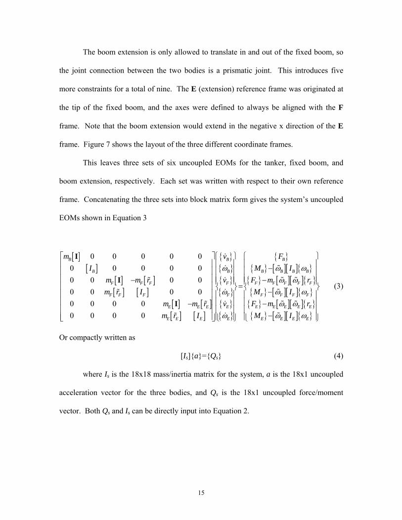
The boom extension is only allowed to translate in and out of the fixed boom, so

the joint connection between the two bodies is a prismatic joint. This introduces five

more constraints for a total of nine. The E (extension) reference frame was originated at

the tip of the fixed boom, and the axes were defined to always be aligned with the F

frame. Note that the boom extension would extend in the negative x direction of the E

frame. Figure 7 shows the layout of the three different coordinate frames.

This leaves three sets of six uncoupled EOMs for the tanker, fixed boom, and

boom extension, respectively. Each set was written with respect to their own reference

frame. Concatenating the three sets into block matrix form gives the system’s uncoupled

EOMs shown in Equation 3

[ ][ ]

[ ] [ ][ ] [ ]

[ ] [ ][ ] [ ]

{ }{ }{ }{ }{ }{ }

{ }{ } [ ][ ]{ }{ } [ ][ ]{ }{ } [ ][ ]{ }{ } [ ][ ]{ }{ } [ ][ ]{ }

0 0 0 0 00 0 0 0 00 0 0 00 0 0 00 0 0 00 0 0 0

BBB

B B B BBB

F F F F FFF F F

F F F FFF F F

E E E E EEE E E

E E E EEE E E

FvmM II

F m rvm m rM Im r I

F m rvm m rM Im r I

ω ωωω ωω ωωω ωω ωω

⎡ ⎤ ⎧ ⎫⎧ ⎫⎢ ⎥ ⎪ ⎪⎪ ⎪ −⎢ ⎥ ⎪ ⎪⎪ ⎪⎢ ⎥ ⎪ ⎪⎪ ⎪ −− ⎪ ⎪ ⎪ ⎪=⎢ ⎥⎨ ⎬ ⎨ ⎬−⎢ ⎥⎪ ⎪ ⎪⎢ ⎥⎪ ⎪ ⎪ −−⎢ ⎥⎪ ⎪ ⎪

−⎢ ⎥⎪ ⎪ ⎪⎩ ⎭ ⎩⎣ ⎦

I

I

I⎪⎪⎪⎪⎭

(3)

Or compactly written as

[Is]{a}={Qs} (4)

where Is is the 18x18 mass/inertia matrix for the system, a is the 18x1 uncoupled

acceleration vector for the three bodies, and Qs is the 18x1 uncoupled force/moment

vector. Both Qs and Is can be directly input into Equation 2.

15

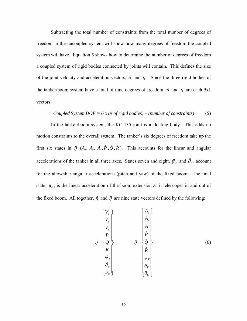
Subtracting the total number of constraints from the total number of degrees of

freedom in the uncoupled system will show how many degrees of freedom the coupled

system will have. Equation 5 shows how to determine the number of degrees of freedom

a coupled system of rigid bodies connected by joints will contain. This defines the size

of the joint velocity and acceleration vectors, η and η . Since the three rigid bodies of

the tanker/boom system have a total of nine degrees of freedom, η and η are each 9x1

vectors.

Coupled System DOF = 6 x (# of rigid bodies) – (number of constraints) (5)

In the tanker/boom system, the KC-135 joint is a floating body. This adds no

motion constraints to the overall system. The tanker’s six degrees of freedom take up the

first six states in η (Ax, Ay, Az, , ,P Q R ). This accounts for the linear and angular

accelerations of the tanker in all three axes. States seven and eight, Fψ and Fθ , account

for the allowable angular accelerations (pitch and yaw) of the fixed boom. The final

state, Eu , is the linear acceleration of the boom extension as it telescopes in and out of

the fixed boom. All together, η and η are nine state vectors defined by the following:

xx

yy

zz

F F

F F

E E

AVAVAVPP

QR

QR

u u

η η

ψ ψθ θ

⎧ ⎫⎧ ⎫⎪ ⎪⎪ ⎪⎪ ⎪⎪ ⎪⎪ ⎪⎪ ⎪⎪ ⎪⎪ ⎪⎪ ⎪⎪ ⎪⎪ ⎪⎪ ⎪= =⎨ ⎬ ⎨ ⎬

⎪ ⎪ ⎪ ⎪⎪ ⎪ ⎪ ⎪⎪ ⎪ ⎪ ⎪⎪ ⎪ ⎪ ⎪⎪ ⎪ ⎪ ⎪⎪ ⎪ ⎪⎩ ⎭ ⎩ ⎭

⎪

(6)

16

η will be input into Equation 2 first according to the initial condition of each

state, and then will be updated at each time step throughout the simulation. η is the

vector that will be obtained by solving Equation 2.

The overall size of the velocity transformation matrix, B, is determined from the

coupled tanker/boom system’s degrees of freedom, and the total number of degrees of

freedom in the uncoupled system. The coupled system’s degrees of freedom defined

above determines the total number of columns in the B matrix and corresponds to the

length of the vectors in Equation 6. The number of rows in B can be found by examining

the length of the acceleration vector a in Equation 4. This vector represents all directions

of motion available in the uncoupled system. The coupled tanker/boom system has nine

degrees of freedom and eighteen uncoupled degrees of freedom. Therefore, the velocity

transformation matrix is an 18x9 matrix.

Each joint type has a corresponding block matrix that fits into the velocity

transformation matrix, B. The size of that block is determined by the joint type. The

rows of the block will always be determined by the six unconstrained degrees of freedom.

The number of columns equals the allowable degrees of freedom defined by a particular

joint type. The tanker as a floating body has no constraints, so it will be a 6x6 block.

The fixed boom (universal joint) has two degrees of freedom and creates a 6x2 block.

The boom extension a single degree of freedom and will be a 6x1 block.

17

“The position of these block matrices within the velocity transformation matrix is

determined by the order in which the bodies are connected, and by the type of joint that

connects the bodies” (11:7). For the tanker/boom system, the velocity transformation

matrix will be in the form of Equation 7.

0 0

0BB

FB FF

EB EF EE

FB F U

F U P

⎛ ⎞⎜= ⎜⎜ ⎟⎝ ⎠

⎟⎟ (7)

where the Fxx (floating) blocks are 6x6, the Uxx (universal) blocks are 6x2 and the Pxx

(prismatic) blocks are 6x1. The block’s order of placement can be seen by looking from

right to left at the bottom row of B, “the boom extension is connected to the fixed boom

by a prismatic joint, the fixed boom is connected to the tanker by a universal joint, and

the tanker is a floating body” (4:7). The contents of the respective blocks contain the

required direction cosine matrices, position vectors, and rotation axes for going between

the different reference frames. Equation 8 shows the block matrices for the bottom row

of B.

(8) /

0

EI EB BE B

EB EB

C C rF

C⎛ ⎞−

= ⎜ ⎟⎝ ⎠

0 0EB B EF FEFU

C n C nψ θ

⎛ ⎞= ⎜ ⎟⎝ ⎠ 0

UE

EE

nP

⎛ ⎞= ⎜ ⎟⎜ ⎟⎝ ⎠

With all the blocks in place, Equation 7 can be directly input into Equation 2. The

remaining unknown piece of Equation 2 is the acceleration transformation matrix, B ,

which is the time derivative of the velocity transformation matrix, B.

18

As mentioned in Chapter 1, the Kunz/Smith boom model based on these EOMs

was developed in Matlab. The EOMs were written in first order form to ensure

compatibility with Matlab’s differential equation solution functions. The model was

validated for uncoupled boom motion against both the AFIT and BOPTT model.

The AFRL KC-135 Model

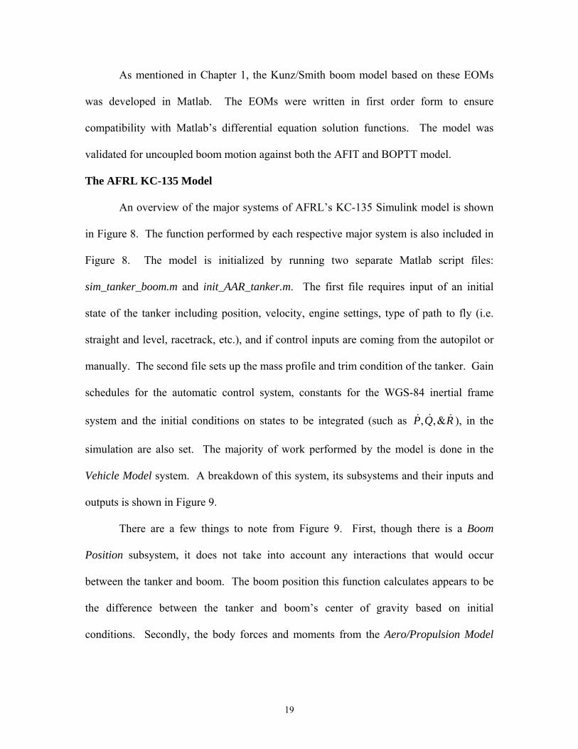
An overview of the major systems of AFRL’s KC-135 Simulink model is shown

in Figure 8. The function performed by each respective major system is also included in

Figure 8. The model is initialized by running two separate Matlab script files:

sim_tanker_boom.m and init_AAR_tanker.m. The first file requires input of an initial

state of the tanker including position, velocity, engine settings, type of path to fly (i.e.

straight and level, racetrack, etc.), and if control inputs are coming from the autopilot or

manually. The second file sets up the mass profile and trim condition of the tanker. Gain

schedules for the automatic control system, constants for the WGS-84 inertial frame

system and the initial conditions on states to be integrated (such as ), in the

simulation are also set. The majority of work performed by the model is done in the

Vehicle Model system. A breakdown of this system, its subsystems and their inputs and

outputs is shown in Figure 9.

, ,&P Q R

There are a few things to note from Figure 9. First, though there is a Boom

Position subsystem, it does not take into account any interactions that would occur

between the tanker and boom. The boom position this function calculates appears to be

the difference between the tanker and boom’s center of gravity based on initial

conditions. Secondly, the body forces and moments from the Aero/Propulsion Model

19

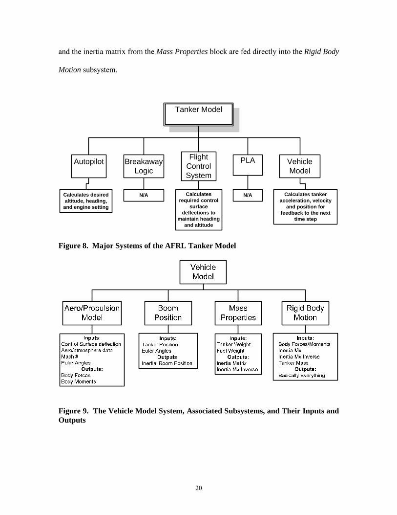
and the inertia matrix from the Mass Properties block are fed directly into the Rigid Body

Motion subsystem.

Tanker Model

Autopilot BreakawayLogic

Flight ControlSystem

VehicleModel

PLA

Calculates desired altitude, heading,

and engine setting

Calculates required control

surface deflections to

maintain heading and altitude

Calculates tanker acceleration, velocity

and position for feedback to the next

time step

N/A N/A

Figure 8. Major Systems of the AFRL Tanker Model

Figure 9. The Vehicle Model System, Associated Subsystems, and Their Inputs and Outputs

20

The Rigid Body Motion module takes the inputs and solves Equation 1 for the

tanker’s acceleration vector. The linear accelerations are integrated twice to get velocity

and position, respectively. The angular accelerations are integrated once to find the

angular rates. These are fed back through the system. The tanker Euler angles, inertial

position and velocity vectors are calculated from quaternions. Many other variations of

these states are also calculated and set up for feedback through the system or output to a

specified location, but are not discussed here because they are not important to the effort

of creating a coupled model. An overview of Rigid Body Motion’s subsystems can be

seen in Figure 10.

There are some points to note in Figure 10 as well. The quaternion and angular

velocity vector coming out of the Equations of Motion block are both fed back to the

Form Accelerations block and fed forward to the Alternate States block. The

acceleration vectors calculated from the Form Accelerations block are fed forward to the

Equations of Motion subsystem. The Equations of Motion block is not exactly as it

seems; its only function is to integrate the accelerations coming out of the Form

Accelerations block. The EOMs are actually solved in the Form Accelerations module.

21

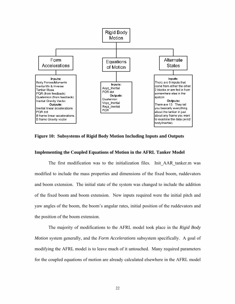
Figure 10: Subsystems of Rigid Body Motion Including Inputs and Outputs

Implementing the Coupled Equations of Motion in the AFRL Tanker Model The first modification was to the initialization files. Init_AAR_tanker.m was

modified to include the mass properties and dimensions of the fixed boom, ruddevators

and boom extension. The initial state of the system was changed to include the addition

of the fixed boom and boom extension. New inputs required were the initial pitch and

yaw angles of the boom, the boom’s angular rates, initial position of the ruddevators and

the position of the boom extension.

The majority of modifications to the AFRL model took place in the Rigid Body

Motion system generally, and the Form Accelerations subsystem specifically. A goal of

modifying the AFRL model is to leave much of it untouched. Many required parameters

for the coupled equations of motion are already calculated elsewhere in the AFRL model

22

and in turn only have to be routed to the correct place. For example, the tanker’s body

forces and moments and the mass/inertia matrix as calculated by the AFRL model were

left alone. Those values are needed to complete the coupled EOMs, but there was no

need to build an entirely new function to compute them. Instead, they were just rerouted

and concatenated into the coupled EOMs. Other parameters that are created by the

coupled EOMs, such as the nine state joint velocity and position vectors, must be fed

back during each time step.

The primary means of modification was placing embedded Matlab functions in

the Form Accelerations subsystem. Embedded Matlab functions are basically standalone

Simulink blocks written in the Matlab language. There is a limited availability of Matlab

tools usable in embedded function. For example, dynamically sizing an array inside a

loop is not allowed. The size of the variable must be defined first, and once that size is

assigned, it cannot change. The functions can take in and output any number of one or

two dimensional arrays defined by the user. Table 2 shows the embedded functions

added to the AFRL model, and a short discussion of each will follow. Code for the

embedded functions can be seen in Appendix C.

23

Table 2. List of Embedded Functions and their purpose

Function Purpose

TankerMass Generate the 6x6 Mass/Inertia Matrix of the Tanker Generate rhs of Tanker's 6x1 Force/Moment Vector

FixedBoom

Generate the 6x6 Mass/Inertia Matrix of the Fixed Boom Generate rhs of Fixed Boom's 6x1 Force/Moment Vector

BoomExt

Generate the 6x6 Mass/Inertia Matrix of the Boom Extension Generate rhs of Boom Extension's 6x1 Force/Moment Vector

Uncoupled18x18 Concatenate the 3 6x6 Mass/Inertia matrices into the 18x18 system Mass/Inertia Matrix Is

FixedBoomDrag_Gravity Calculate the aerodynamic and gravitational force and moment contribution of the Fixed Boom

LeftRuddevator Calculate the aerodynamic and gravitational force and moment contribution of the Left Ruddevator

RightRuddevator Calculate the aerodynamic and gravitational force and moment contribution of the Right Ruddevator

BoomExtension_Drag_Gravity Calculate the aerodynamic and gravitational force and moment contribution of the Boom Extension

VelocityTransformation Calculate the Velocity Transformation Matrix, B

AccelerationTransformations Calculate the Acceleration Transformation Matrix, B_dot

Combined Concatenate all the body and gravitational forces/moments to form the system's 18x1 Force/Moment vector

RHS_I_Bdot_eta performs [Is]*[Bdot]*[ηdot]

etadoubledot solves the coupled EOMs for the 9 state joint acceleration vector

24

A total of 13 embedded functions were added to the Form Accelerations

subsystem. Since most of the embedded functions share a majority of required inputs, a

single vector was created to serve as their input. This helped clean up the appearance of

the new Form Accelerations block and made signal routing much easier. .

TankerMass: Inputs to this function were the tanker’s mass and inertia matrix as

calculated by the original model. Basically, this took Simulink’s version the tanker’s

inertia matrix, which was a six component vector containing the mass moment of inertia

for each principal direction, and formed the 6x6 mass/inertia matrix of the tanker. Also

the [ ][ ]{ }B B BIω ω portion of the tanker’s section of Qs in Equation 4 was calculated and

output.

FixedBoom: Inputs were the tanker’s angular velocity and the pitch/yaw position

and rate of the boom. It calculated the fixed boom’s mass/inertia matrix, along with the

[ ][ ]{ }F F F Fm rω ω and [ ][ ]{ }F F FIω ω portions of Qs corresponding to the fixed boom.

BoomExt: Inputs were the boom extension’s position, the tanker’s angular

velocity and the pitch/yaw position and rate of the boom. It calculated the boom

extension’s mass/inertia matrix, along with the [ ][ ]{ }E E E Em rω ω and [ ][ ]{ }E E EIω ω

portions of Qs corresponding to the boom extension.

Uncoupled18x18: Took in the three 6x6 mass/inertia matrices and the three 6x1

right portions of Qs. Assembled the 18x18 mass/inertia matrix for the system and the

18x1 right side of Qs.

25

FixedBoomDragGravity: Inputs to this system include the tanker’s inertial

velocity vector and Euler angles, as well as the fixed boom’s pitch/yaw attitude and rates.

The incremental aerodynamic forces on the fixed boom were calculated using the drag

relationship and integrated from the boom tip to the boom pivot. The fixed boom was

modeled as a cylinder of varying diameter and the drag coefficient was found from the

cylinder’s relationship to the local Reynold’s number. This function’s output was the

6x1 aerodynamic and gravitational force/moment vectors of the fixed boom.

LeftRuddevator: Inputs here were the translational and angular velocities and

Euler angles of the tanker and the fixed boom’s pitch/yaw attitude and rates.

Aerodynamic forces were calculated using general aerodynamic strip theory as would be

used on any wing or control surface. An additional coordinate system was needed for

this calculation, and it originated where the ruddevator would intersect the fixed boom

centerline. All three axes initially aligned with those of the F frame. This coordinate

system was then rotated 42o about the x axis to account for the ruddevator dihedral angle.

This rotation puts the left ruddevator on the negative y axis and defines the WL frame.

The local velocity was calculated and the angle of attack was corrected for yawed flow.

With this corrected angle of attack, lift and drag coefficients were calculated and the

incremental forces and moments were calculated across the ruddevator span. The

incremental forces were then integrated from the ruddevator tip inboard. Once the force

and moment contribution of left ruddevator had been calculated in the WL frame, they

were transformed to act at the boom pivot, which is also the origin of the F frame.

26

RightRuddevator: Same inputs and calculations performed as in the

LeftRuddevator function, but this time the coordinate system was rotated -42o about the x

axis to form the WR frame. In turn, the positive y direction went from the origin outboard

to the right ruddevator tip, and the incremental forces and moments were integrated from

inboard to outboard. The ruddevator reference frames are shown in Figure 11.

WLz

-WLy

WRz

WRy

Figure 11. Ruddevator Coordinate Frames (1)

BoomExtension_Drag_Gravity: Aerodynamic forces and moments for the

boom extension were calculated in the same manner as the elliptical portion of the fixed

boom, with the exception that the boom extension has a fixed diameter. Obviously, if the

boom extension is completely inside the fixed boom, it adds no drag to the system. If the

boom extension has telescoped out of the fixed boom, the incremental drag forces are

calculated and then integrated from the boom extension’s tip to the tip of the fixed boom.

VelocityTransformation: Takes in the tanker and fixed boom position angles

and the boom extension’s position. Computes the floating, universal and prismatic

blocks of Equation 7 and then assembles them into the 18x9 velocity transformation

matrix B.

27

AccelerationTransformation: Takes in the tanker and fixed boom attitudes and

the pitch/yaw rate of the fixed boom. Computes the derivative of the velocity

transformation matrix, which is the acceleration transformation matrix B .

Combined: Takes in the tanker body forces and moments originally calculated

by the AFRL model, and all the aerodynamic and gravitational forces/moments for the

fixed boom, ruddevators and boom extension. Recall that the Left/Right Ruddevator

function transformed their forces and moments to act at the boom pivot, which is the

origin of the F reference frame. Here, both ruddevator forces and moments are added to

the forces and moments for the fixed boom. Once that was done, everything was

concatenated into an 18x1 force vector, which is the left portion of Qs from Equation 4.

RHS_I_Bdot_eta: Takes in Is from the Uncoupled18x18 function, B from the

AccelerationTransformation function, the joint velocity vector, η that was fed back from

the Equations of Motion system from the AFRL model, and the tanker’s inertial velocity

vector. Computes the Is B η portion of Equation 2.

etadoubledot: Takes in Is from the Uncoupled18x18 function, the fully

assembled 18x1 Qs vector, and the velocity transformation matrix, B from the

VelocityTransformation function. Computes the joint acceleration vector, η , of the

coupled tanker/boom system. This is the final solution to Equation 2, the EOMs that

were derived to couple the tanker and boom, at a particular time step.

After coming out of the etadoubledot function, the joint acceleration vector is

then fed forward to the Equations of Motion system. Originally, there were two Simulink

integration block systems in the Equations of Motion system; one for the linear and

28

another for the angular accelerations of the tanker. Prior to entering the Equations of

Motion system, the tanker’s linear accelerations were converted to the inertial frame. In

order to keep the original model going with all its calculations involving the various

forms of the basic data, the linear and angular accelerations of the tanker (the first 6

states of η ) were extracted from η . The tanker’s linear accelerations were converted to

the inertial frame and then they along with the tanker’s angular accelerations were sent

through the AFRL model’s two original integration block systems. Inside the Equations

of Motion system, a third Simulink integration block system was added and set up to

receive η , integrate it twice and extract the joint velocity and position vectors that were

required for feedback through the Form Accelerations system. The modified portions of

the AFRL Simulink model can be seen in Appendix A

29

III Data Analysis

Overview

Data collection and analysis for this thesis basically involved performing

simulations of the new model, and comparing those results to similar simulations

performed using the Kunz/Smith boom model and the AFRL tanker model. Of particular

interest was investigating the motion of the boom and tanker, and taking note to see if the

newly developed equations of motion did exhibit any coupling tendencies between the

tanker and boom. For final validation, simulation results were compared to data recorded

during a flight test.

The first evaluation of the new coupled Simulink model was to run the simulation

with the tanker limited to unaccelerated, straight and level flight. This effectively puts

the tanker back on the assumed rigid rail of the original AFRL model because the tanker

will not be able to respond to any boom motion. Everything in the tanker’s acceleration

and velocity vector, except the tanker’s initial velocity, must be forced to zero in order to

accomplish this. These conditions replicate the comparison of the Kunz/Smith boom to

the BOPTT and AFIT boom models. Comparisons between the new model and the

Kunz/Smith model were used for initial validation of boom motion in the new model.

Boom response to symmetric and asymmetric ruddevator step deflections will be

investigated. In both cases, boom motion should be very similar in this series of

simulations. Since the Kunz/Smith model has already been validated as an effective

representation of boom behavior, this test will serve to validate the behavior of the new

model’s boom.

30

The second step in model validation will study the effect of coupling the boom

and tanker. If the two bodies have in fact been effectively coupled, there should be small,

but noticeable changes in the behavior of the tanker and boom. A comparison of tanker

motion between the AFRL tanker model and the coupled model will show any effects the

boom has on the tanker. The two models were compared in straight and level flight, and

no control inputs were commanded to the boom in the coupled simulation. To investigate

the effect of the tanker on boom motion, the coupled model simulation will be performed

twice; once with the tanker constrained to straight and level flight, and then with no

motion constraints placed on the tanker. This test will show the tanker’s coupling effect

on the boom. There should be no large differences in response for any of these test cases.

There should be a settling period involved with the coupled model in all attitudes, but

tanker and boom motion should generally follow that of the existing models.

To investigate the tanker effects on controlled boom motion, the six degree

symmetric and asymmetric ruddevator deflection tests will be repeated with the steady

level flight constraint removed. These results will then be compared to the previous

results of the same simulation performed with the steady flight constraint in place.

To study the effects of commanded boom motion on the tanker, a ten degree

symmetric and asymmetric ruddevator deflection will be commanded in the fully coupled

model. A comparison will be made between this simulation, and simulation performed

by the AFRL and coupled model with no control inputs.

31

Final validation will come from comparison of the coupled model to existing

flight test data recorded during a series of flight tests. The test cases to be examined will

compare tanker and boom response to a schedule of ruddevator deflections. If

simulations from the new model behave with consistency and can resemble the responses

of the available data, then the new coupled model can be validated as a reasonable tool

with which to study the motion of the tanker/boom system.

Test Scenario Setup

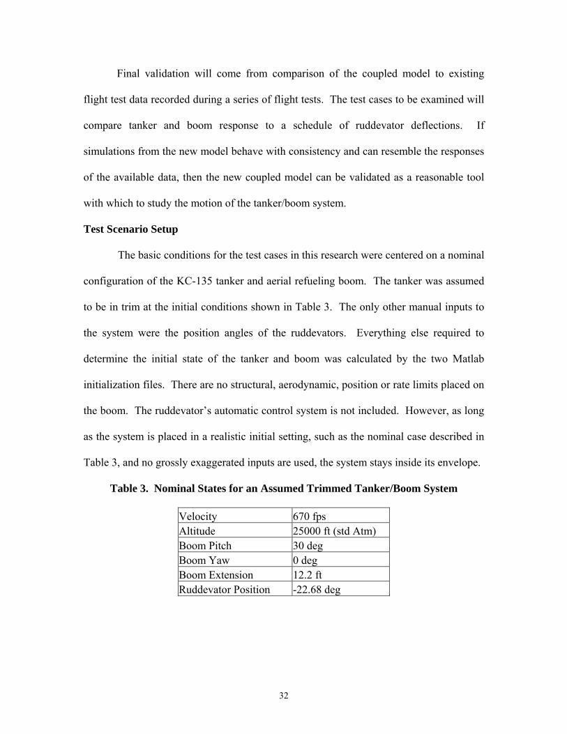
The basic conditions for the test cases in this research were centered on a nominal

configuration of the KC-135 tanker and aerial refueling boom. The tanker was assumed

to be in trim at the initial conditions shown in Table 3. The only other manual inputs to

the system were the position angles of the ruddevators. Everything else required to

determine the initial state of the tanker and boom was calculated by the two Matlab

initialization files. There are no structural, aerodynamic, position or rate limits placed on

the boom. The ruddevator’s automatic control system is not included. However, as long

as the system is placed in a realistic initial setting, such as the nominal case described in

Table 3, and no grossly exaggerated inputs are used, the system stays inside its envelope.

Table 3. Nominal States for an Assumed Trimmed Tanker/Boom System

Velocity 670 fps Altitude 25000 ft (std Atm) Boom Pitch 30 deg Boom Yaw 0 deg Boom Extension 12.2 ft Ruddevator Position -22.68 deg

32

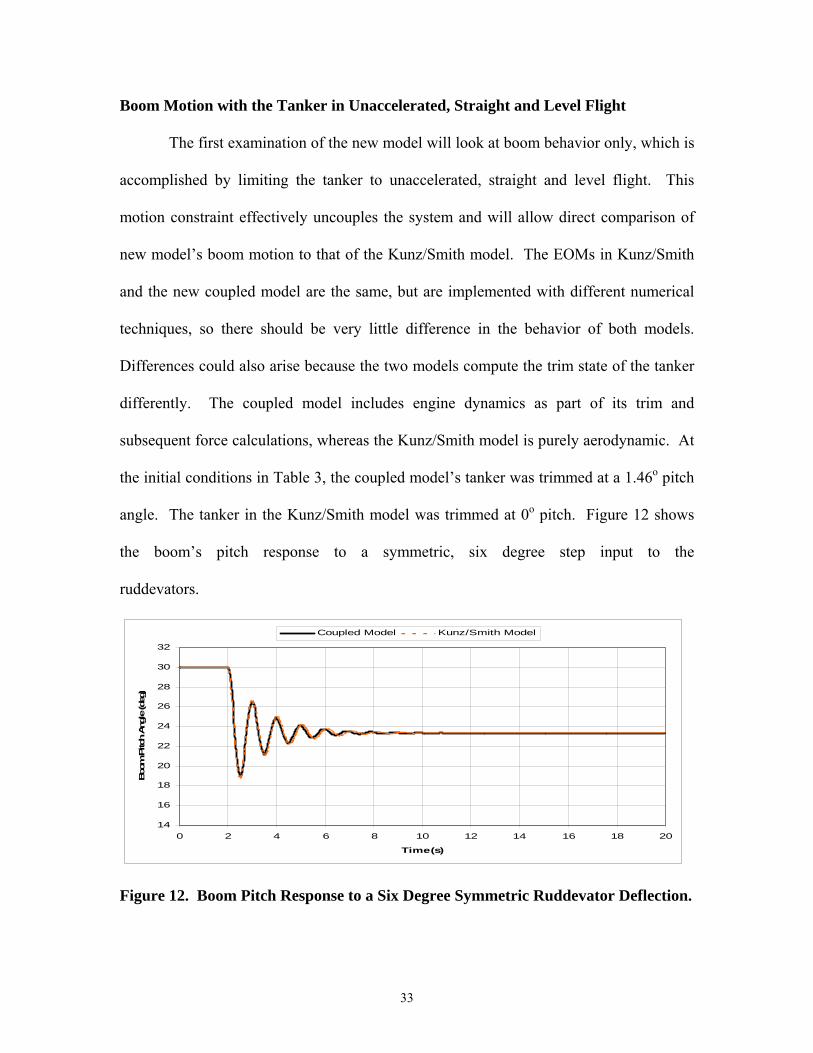
Boom Motion with the Tanker in Unaccelerated, Straight and Level Flight

The first examination of the new model will look at boom behavior only, which is

accomplished by limiting the tanker to unaccelerated, straight and level flight. This

motion constraint effectively uncouples the system and will allow direct comparison of

new model’s boom motion to that of the Kunz/Smith model. The EOMs in Kunz/Smith

and the new coupled model are the same, but are implemented with different numerical

techniques, so there should be very little difference in the behavior of both models.

Differences could also arise because the two models compute the trim state of the tanker

differently. The coupled model includes engine dynamics as part of its trim and

subsequent force calculations, whereas the Kunz/Smith model is purely aerodynamic. At

the initial conditions in Table 3, the coupled model’s tanker was trimmed at a 1.46o pitch

angle. The tanker in the Kunz/Smith model was trimmed at 0o pitch. Figure 12 shows

the boom’s pitch response to a symmetric, six degree step input to the

ruddevators.

14

16

18

20

22

24

26

28

30

32

0 2 4 6 8 10 12 14 16 18 20

Time(s)

Boo

m P

itch

Angl

e (d

eg)

Coupled Model Kunz/Smith Model

Figure 12. Boom Pitch Response to a Six Degree Symmetric Ruddevator Deflection.

33

The step was commanded at two seconds. As expected, the Kunz/Smith and

coupled models basically mirror each other. The coupled model tracks the motion of the

Kunz/Smith model, but has slightly higher frequency and damping. This can be

explained by the differences in numerical techniques used. To accomplish the required

integration of incremental forces and moments on the fixed boom, ruddevators and boom

extension, Kunz and Smith used the Matlab function quadv, which is based on the

adaptive Simpson’s rule for quadrature. The new Simulink model uses an integration

routine based on the trapezoidal rule to perform the same operations.

In addition, when determining the incremental lift and drag coefficients on the

ruddevators, Kunz and Smith use a two-dimensional table lookup and interpolation based

on local the angle of attack and Mach number along the span of the ruddevators. Due to

limitations involved with using embedded Matlab functions in a Simulink model, this

was reduced to a one dimensional interpolation in the coupled model. Ruddevator lift

and drag coefficient data was available in tabular form at Mach numbers of 0, 0.2, 0.3,

0.4, 0.5, 0.6, 0.8, and 1. The new model calculates the local Mach number and angle of

attack along the ruddevator span, selects the closest Mach number table available, and

then the coefficients are determined by a linear interpolation based on the local angle of

attack. Therefore, the ruddevators in the coupled model generated slightly different

forces than the Kunz/Smith model.

34

The forces generated by the ruddevators in the coupled model were about 7-8%

larger than those of Kunz/Smith, and in turn the new model’s ruddevators have more

control authority than those of the Kunz/Smith model. Boom yaw response is not

examined in this case because the maximum yaw motion is on the order of 10-6 degrees.

Next, a six degree asymmetric step deflection was commanded to the

ruddevators. For the case in Figure 13, the left ruddevator deflection was a negative six

degrees (from nominal to -28.68o), and the right was positive (from nominal to -16.68o).

Again, the coupled model has a higher frequency and damping, but in this case, the initial

response is of larger amplitude and the boom eventually converges to a slightly higher

pitch angle than that of the Kunz/Smith model. This is where the different initial trim

states of the models can be seen. In the boom pitch angle plot of Figure 13, the coupled

model’s boom starts in its nominal 30o pitch down state and initially starts to climb in an

effort to find its true trim state. Kunz and Smith note that in the coupled system, the

ruddevators help force the boom down when it is in a yawed state (4:9). This occurs

during the initial response to the ruddevator deflection where the coupled model’s more

authoritative controls force the boom further down.

Simulation results for boom behavior in the new model match that of the

Kunz/Smith. There are slight, but acceptable, differences in motion due to the different

numerical techniques used. This proves that the new model adequately produces

uncoupled boom motion similar to the existing and previously verified models.

35

29

29.5

30

30.5

31

31.5

0 2 4 6 8 10 12 14 16 18 20

Time (s)

Boom

Pitc

h An

gle

(deg

)

Coupled Kunz/Smith

0

2

4

6

8

10

12

14

16

0 2 4 6 8 10 12 14 16 18 20

Time (s)

Boom

Yaw

Ang

le (d

eg)

Coupled Kunz/Smith

Figure 13. Boom Yaw and Pitch Response to a Six Degree Asymmetric Ruddevator Deflection.

36

The Effect of Coupling the Tanker and Boom

To investigate the effect of coupling the boom to the tanker, the tanker in the

coupled model must be removed from the unaccelerated, steady flight constraint. With

that restriction gone, a simulation was performed using no ruddevator control inputs to

look at the changes in both boom and tanker behavior. To study the effect on the tanker,

these results were compared to a simulation performed using the AFRL tanker model. To

study the coupling effect on the boom, the results from this simulation were compared to

those of the coupled model with the steady flight restriction still on the tanker.

The coupling effect of the boom and tanker can be seen in Figure 14 and Figure

15. Boom effects on the tanker are easily noticeable. First is the initial transient of the

coupled model as the tanker adjusts to the boom. It quickly settles into a slightly more

nose up attitude. Afterwards, the coupled tanker continues to remain in a more nose up

attitude. This is because the nose down moment caused by the drag force on the boom is

overcome by the nose up moment generated by its weight. The difference in the tanker

pitch angle is not significant, but the fact that there is a difference shows that coupling

between the boom and tanker is taking place in the new model and that this change

conforms to the expected physics of the situation.

37

1

1.1

1.2

1.3

1.4

1.5

1.6

1.7

0 20 40 60 80 100 1

Time (s)

Tank

er P

itch

Ang

le (d

eg)

20

AFRL Coupled

Figure 14. Tanker Pitch Angle Comparison from the Coupled and AFRL Model

29.5

29.6

29.7

29.8

29.9

30

30.1

30.2

30.3

30.4

30.5

0 20 40 60 80 100 1

Time (s)

Boom

Pitc

h An

gl

20

e

US&LF Coupled

Figure 15. Boom Pitch Angle Comparison: Coupled and Steady, Level Flight Constrained

38

Figure 15 shows the effect of the tanker on the boom. The tanker appears to have

very little impact on the boom. Again, there is the initial transient followed by the boom

settling in a slightly more pitch down attitude. Also of note is the pitch motion of the

boom is measured with respect to the tanker centerline. As expected, the simulation with

the steady level flight constraint showed no reaction to changes in tanker attitude. For

the coupled model, recall that positive boom pitch is measured in degrees down from the

aircraft centerline. After the initial transient (t = 0-8 sec), the tanker pitch attitude noses

down and the boom pitches up. Some of this increase in boom pitch is likely related to

the fact the reference frame for the measurement moved upwards, but the value of the

tanker pitch and boom pitch changes are not the same. At the maximum change, tanker

pitch decreased by ~0.2o while boom pitch only increased ~0.1o. This indicates that the

ruddevators are pushing the boom in the opposite direction. This trend continues in both

directions as the tanker pitch settles out. The change in trim is rather small, but again, the

fact that there was any change shows that the dynamics of the tanker and boom are in

indeed interacting.

The results of this test are another good sign for the viability of the new model.

They showed that there were in fact dynamic interactions taking place between the tanker

and boom. Behavior changes were small but noticeable, and in agreement with the

expected physics of the situation.

39

Tanker Effects on Boom Motion with Boom Control Inputs

To find out what effects the tanker has on boom motion, the first two simulations

(six degree symmetric and asymmetric ruddevator step inputs) were repeated with the

unaccelerated, steady flight constraint removed.

Figure 16 shows that the tanker has a negligible effect on boom motion when a

symmetric ruddevator deflection is commanded. The coupled boom also shows the same

initial transient as the boom and tanker begin to settle. Eventually, the boom settles out

to a more increased pitch down angle than US&LF, but not enough to have any real

effect on the boom motion.

18

20

22

24

26

28

30

32

0 2 4 6 8 10 12 14 16 18 20

Time (s)

Boom

Pitc

h An

gle

(deg

)

Coupled US&LF

Figure 16. Comparison of Boom Pitch Response to a Six Degree Symmetric Ruddevator Deflection.

40

Coupled boom response to a six degree asymmetric control input can be seen in

Figure 17. Again, the tanker does not make any significant difference in the yaw motion

of the boom. The initial effect of coupling the tanker and boom can again be seen in the

boom’s pitch transient during the two seconds before the ruddevator input is commanded.

The coupled boom’s pitch trims out about 0.25o more pitch down than the US&LF case.

These results are also promising. The tanker is exhibiting an influence, however

small, on the motion of the boom. Of note is that the no matter the input, the boom

trimmed out to a slightly increased pitch angle. This is expected based on the results

shown in Figure 15.

41

29

29.5

30

30.5

31

31.5

0 2 4 6 8 10 12 14 16 18 20

Time (s)

Boom

Pitc

h An

gle

(deg

)

Coupled US&LF

0

2

4

6

8

10

12

14

16

0 2 4 6 8 10 12 14 16 18 20

Time (s)

Boom

Yaw

Ang

le (d

eg)

Coupled US&LF

Figure 17. Comparison of Boom Pitch and Yaw Response to a Six Degree Symmetric Ruddevator Deflection.

42

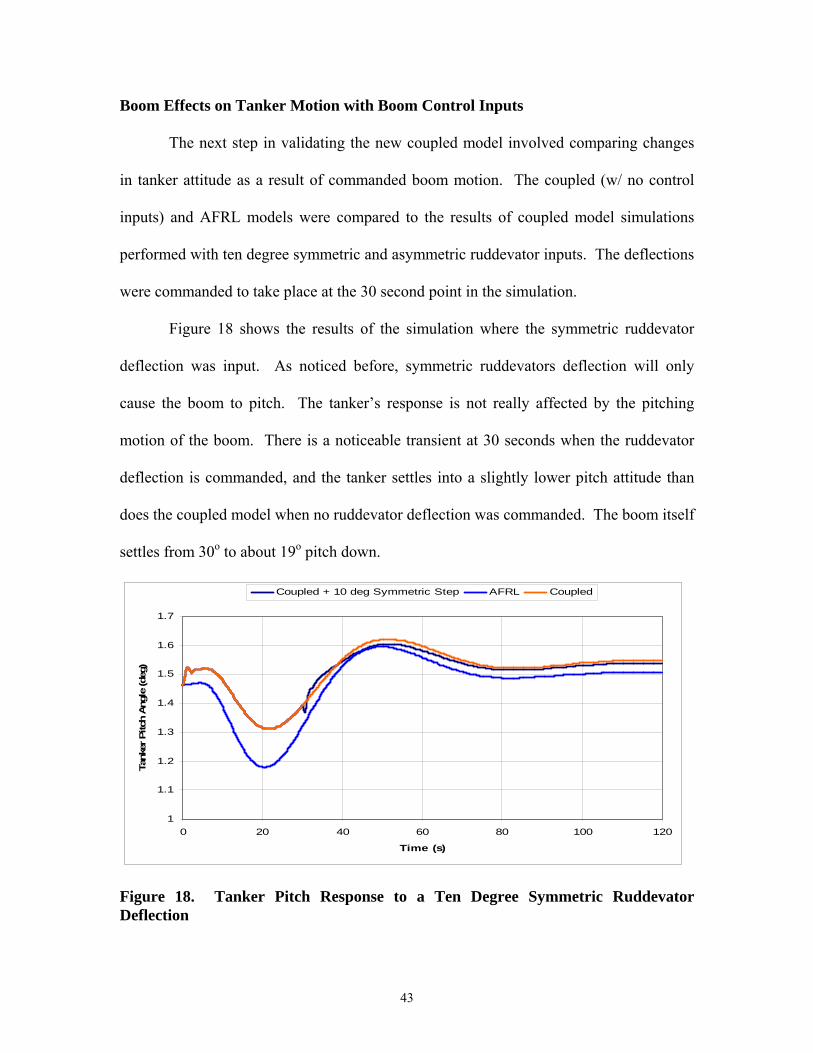
Boom Effects on Tanker Motion with Boom Control Inputs

The next step in validating the new coupled model involved comparing changes

in tanker attitude as a result of commanded boom motion. The coupled (w/ no control

inputs) and AFRL models were compared to the results of coupled model simulations

performed with ten degree symmetric and asymmetric ruddevator inputs. The deflections

were commanded to take place at the 30 second point in the simulation.

Figure 18 shows the results of the simulation where the symmetric ruddevator

deflection was input. As noticed before, symmetric ruddevators deflection will only

cause the boom to pitch. The tanker’s response is not really affected by the pitching

motion of the boom. There is a noticeable transient at 30 seconds when the ruddevator

deflection is commanded, and the tanker settles into a slightly lower pitch attitude than

does the coupled model when no ruddevator deflection was commanded. The boom itself

settles from 30o to about 19o pitch down.

1

1.1

1.2

1.3

1.4

1.5

1.6

1.7

0 20 40 60 80 100 120

Time (s)

Tank

er P

itch

Angl

e (d

eg)

Coupled + 10 deg Symmetric Step AFRL Coupled

Figure 18. Tanker Pitch Response to a Ten Degree Symmetric Ruddevator Deflection

43

Next was a comparison of simulations performed with an asymmetric ruddevator

deflection. For this particular simulation, it is important to clearly understand the final

state of the tanker/boom system at the end of the simulation. The boom moved from the

30o pitch and 0o yaw position to 19o pitch and 15o yaw. This places the boom in a higher

pitch attitude in the freestream on the left side of the aircraft. The tanker’s pitch attitude

behaves almost exactly the same as in previous tests, but here is where we see the first

changes to the tanker’s yaw and roll attitude due to the boom. The tanker ended up with

a slight negative (right wing up) roll attitude and a steadily increasing negative yaw (nose

left) attitude. These results are shown in Figure 19.

The tanker’s pitch response remains virtually unchanged from the symmetric

input case, but did go up a miniscule amount settling a little closer to the final value of

the coupled model with no inputs. The change in the roll and yaw angles is due to the

final placement of the boom in this test case.

As mentioned previously, the boom trims out under the left side of the aircraft.

This adds an extra mass component to the left of the tanker’s center of gravity which in

turn generates a moment that forces the left wing down (a negative roll attitude). In

similar fashion, the drag component of the boom generates a negative yawing moment

(nose left).

44

Coupled + 10deg Asymmetric Step

Figure 19. Tanker Pitch, Roll and Yaw Response to a Ten Degree Asymmetric Ruddevator Deflection

1

1.1

1.2

1.3

1.4

1.5

1.6

1.7

0 20 40 60 80 100 120

Time (s)

Tank

er P

itch

Ang

le (d

eg)

Coupled AFRL

Coupled +10deg Asymmetric Step Coupled AFRL

-0.4

-0.35

-0.3

-0.25

-0.2

-0.15

-0.1

-0.05

0

0.05

0 20 40 60 80 100 120

Time (s)

Tank

er R

oll A

ngle (d

eg)

Coupled +10deg Asymmetric Step Coupled AFRL

-3

-2.5

-2

-1.5

-1

-0.5

0

0.5

0 20 40 60 80 100 120

Time (s)

Tank

er Y

aw A

ngle

(deg

)

45

These results correspond to what should be expected to happen for the

tanker/boom system in this particular configuration. However, the yaw attitude of the

tanker does not settle into a new trim condition, but instead the tanker trims into a steady

level turn to the left.

These tests have shown that the tanker responds to the boom as would be

expected. The changes are not large, but those that occur agree with the physics of the

problem.

Comparison to Flight Test Data

The final validation for the newly developed model will attempt to compare

results obtained from the simulation to flight test data collected for the Air Force in 1998

(3). The data itself is very limited as a comparative tool. No numeric data was available,

only pictures of the time histories for each test are available. Some scales used for the

flight tests do not lend to easy interpretation. For example, the pitch rates generated by

the simulation ranged from -0.1o/s up to 0.1o/s. The scale of the pitch rate time history

ran from -4o/s up to 4o/s. Accordingly, the flight test data hung around zero but could not

be interpreted to make a direct comparison to the simulation results useful. For

comparisons such as that one, a generalization could be made indicating that the

simulation was not generating completely false data, but there was nothing to corroborate

its results. Also, tanker attitude comparisons may be of little use.

46

In the test scenarios examined, the tanker was being flown manually, whereas the

simulation completely relies on the model of the autopilot for tanker control inputs. That

being said, where the flight test data could be interpreted and an effective comparison

made between it and the simulation, it was performed and will be discussed. Otherwise,

items such as the attitude rates of the tanker will not.

The entire scenario of the flight test was not recreated in the simulation. The

scope of the research was only interested in validating the general behavior of this

approach to coupling the tanker and refueling boom. The initial trim condition of the

tanker and boom for the flight test was different from the configuration run in the

simulation. The altitude (~21000 ft) and speed (~622 fps) of the tanker was slightly

lower than that of the nominal case. The tanker’s pitch attitude (2.5o) and weight (240k

lbf) was higher, and the initial position of the boom was a little different from nominal as

well.

For the simulation runs, the tanker/boom system was left in the nominal case of

Table 3. Data from the flight test time histories was manually read and placed into a file

so that comparisons could be made on a single graph. When the simulation data had been

collected and plotted, the flight test data was shifted up or down so that its initial value

would match that of the simulation. From this point, the comparisons of the boom and

tanker behavior trends could be examined.

The two flight test cases to be examined were both quite similar. The tanker and

refueling boom were both initially flying straight and level in a trim configuration. A

series of ruddevator deflections was commanded, and the data acquisition system

measured and recorded time histories for numerous aircraft and boom parameters. Each

47

test case lasted about 80 seconds. The first deflection schedule commanded a series of

symmetric inputs to examine the boom’s pitch behavior. The second was a series of

asymmetric deflections to investigate the boom’s yaw behavior.

The series of ruddevator commands changed the ruddevator control input method

for the simulation. In each of the earlier simulations, the ruddevator position was set

before the simulation started. If necessary, a single step change to this initial position

was made at a desired point in time. Ruddevator deflections from the flight test data

were part of the time histories returned by the data acquisition system. For use in the

simulation, the complete time history of ruddevator position was modeled as a series of

straight lines with respect to time. Distinct points of interest, basically where the

ruddevator position changed slope, were used to generate both a time and position vector

of ruddevator position. These vectors were placed into the embedded functions for the

left and right ruddevator, and transitions between the distinct points were approximated

by a linear interpolation.

The results of the first simulation (symmetric ruddevator deflection) can be seen

in Figure 20. The first chart shows the ruddevator deflection schedule that was

commanded in this test. This delfection schedule was designed to investigate the pitch

response of the boom. The model’s boom pitch motion generally followed the flight test

data. The model moved to greater extremes when the ruddevators were held in place

after a linear deflection. Otherwise, the boom’s pitch changed or leveled out every time

the ruddevators did the same. Here, the differences are not large, and considering the

manual interpretation and shifting of the test data, the general trend of the simulation is

consistent with the flight test. This is not the case with the yaw attitude of the boom.

48

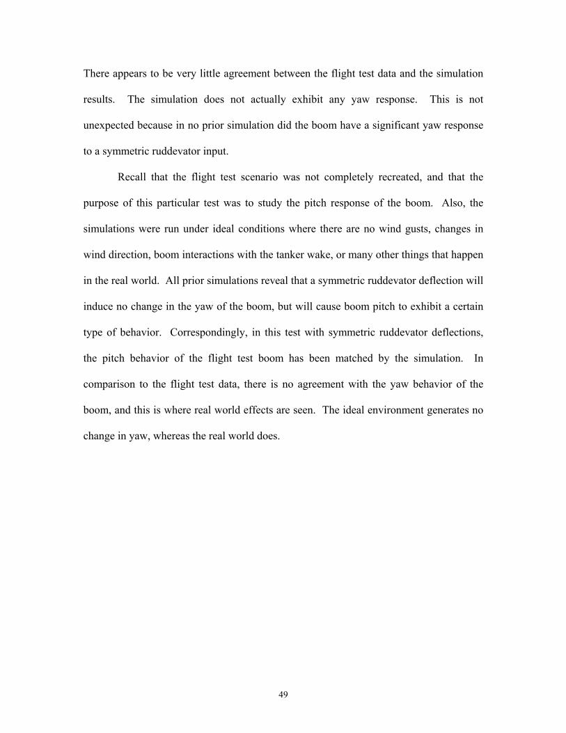
There appears to be very little agreement between the flight test data and the simulation

results. The simulation does not actually exhibit any yaw response. This is not

unexpected because in no prior simulation did the boom have a significant yaw response

to a symmetric ruddevator input.

Recall that the flight test scenario was not completely recreated, and that the

purpose of this particular test was to study the pitch response of the boom. Also, the

simulations were run under ideal conditions where there are no wind gusts, changes in

wind direction, boom interactions with the tanker wake, or many other things that happen

in the real world. All prior simulations reveal that a symmetric ruddevator deflection will

induce no change in the yaw of the boom, but will cause boom pitch to exhibit a certain

type of behavior. Correspondingly, in this test with symmetric ruddevator deflections,

the pitch behavior of the flight test boom has been matched by the simulation. In

comparison to the flight test data, there is no agreement with the yaw behavior of the

boom, and this is where real world effects are seen. The ideal environment generates no

change in yaw, whereas the real world does.

49

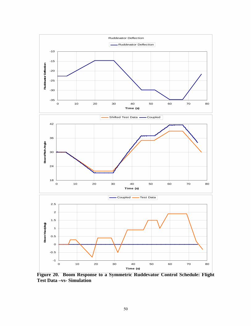
Figure 20. Boom Response to a Symmetric Ruddevator Control Schedule: Flight Test Data –vs- Simulation

18

24

30

36

42

0 10 20 30 40 50 60 70 8

Time (s)

Boom

Pitc

h An

gle

0

Shifted Test Data Coupled

Ruddevator Deflection

-35

Ruddevator Deflection

-3Ru 0

-25

-20

-15

-10

0 10 20 30 40 50 60 70 80

Time (s)

ddev

ator

Def

lect

ion

Coupled Test Data

-1

-0.5

0

0.5

1

1.5

2

2.5

0 10 20 30 40 50 60 70 80

Time (s)

Boo

m Y

aw (d

eg)

50

Figure 21 shows the results of the second simulation. Again, the first chart shows

the ruddevator deflection schedule. This test commanded a series of asymmetric

ruddevator deflections intended to investigate boom yaw response to the commanded

inputs. Just as in the symmetric test case, the off-axis test, which in this case was boom

pitch response, does not correspond very well to the flight test data. On the other hand,

the yaw motion of the boom matched almost perfectly. Again, the extremes of the

motion were a little larger for the simulation than in the flight test data and can be

explained by the manual interpretation and shifting of the test data. Looking closely at

the two specific flight tests, it is apparent that each ruddevator control schedule was

designed to investigate boom behavior for a specific axis and real world interactions

caused the differences in the off-axis behavior.

The overall results of the combined research presented in this chapter corroborate

this. In all previous cases where a symmetric ruddevator deflection was commanded,

there was no effect on the boom’s yaw position. With this information, of the lack of

agreement in boom yaw position in Figure 20 and boom pitch position in figure 21

lessens in importance. What is significant is that the simulation performance did exhibit

the same behaviors as the boom in the flight test when compared to the defined purpose

of the test.

51

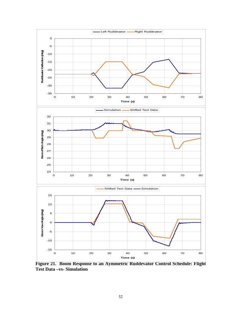
24

25

26

27

28

29

30

31

32

0 10 20 30 40 50 60 70 8

Time (s)

Boom

Pitc

h An

gle

(deg

)

0

Simulation Shifted Test Data

-35

-30

-25

-20

-15

-10

-5

0

0 10 20 30 40 50 60 70 8

Time (s)

Rudd

evat

or D

efle

ctio

n (d

eg)

Figure 21. Boom Response to an Aymmetric Ruddevator Control Schedule: Flight Test Data –vs- Simulation

0

Left Ruddevator Right Ruddevator

-15

-10

-5

0

5

10

15

0 10 20 30 40 50 60 70 8

Time (s)

Boom

Yaw

Ang

le (d

eg)

0

Shifted Test Data Simulation

52

IV. Conclusions and Recommendations

Conclusions

In the KC-135’s nearly 50 years of flight, no simulation has been developed to

model the dynamic interactions of the tanker aircraft and its aerial refueling boom. This

thesis has filled that knowledge gap. Using the EOMs developed by Kunz and Smith in

tandem with AFRL’s model of the KC-135 tanker, the first model to reasonably simulate

the behavior of the tanker and boom as a single, dynamically coupled system has been

developed

After all the simulations have been examined, it is safe to say that this model is a

viable tool to further extend research in the area of AAR. Results obtained from this

model were consistent with those obtained from the established AFRL tanker model and

the Kunz/Smith boom model. The slight behavior differences between the simulations

can mostly be explained by the numerics used to solve the problem.

In the two simulations that were compared to flight test data, it is important to

note that each flight test event was performed to measure either the boom’s pitch or yaw

performance. Symmetric ruddevator deflections tested the pitch motion of the boom, and

the results of the simulation matched the trends of the test data when comparing that

mode of motion. Asymmetric ruddevator deflections tested the yaw behavior of the

boom, and once again, the simulation matched the trends of the test data when comparing

the yaw motion of the boom.

53

The goals for the focus and scope of this research have been reached. There are

certainly improvements that could be made to the model and further testing and

refinement could expand the model’s viability beyond that of a basic research tool. This

study was undertaken to develop and validate a model that coupled the dynamic

interactions between the KC-135 tanker aircraft and its refueling boom, and this goal has

been accomplished.

Suggestions for further Study

Several things could be done to make this model a more valuable tool for AAR

research. The tests run in this thesis centered around a nominal configuration of the

tanker and boom system, so the test envelope should be expanded. Refinements could be

made to improve the accuracy of the simulation and the computational efficiency of the

model could also be improved. Finally a full blown AAR simulation could be developed

by the addition of a receiver aircraft to this model.

Before the model can be considered completely viable, it needs to be thoroughly

examined in conditions other than the nominal case. Racetrack patterns, different tanker

mass and attitude configurations, and different boom attitudes and extension positions

should be studied. If possible, some further tests should be compared to raw flight test

data. Comparisons between the available flight test data and tanker behavior (attitude

and body rates) proved to be virtually non-existent due to limitations of the available

data. Also, any real world position, rate, and aerodynamic limits, along with the

ruddevator control system, should be added to the boom portion of the model.

54

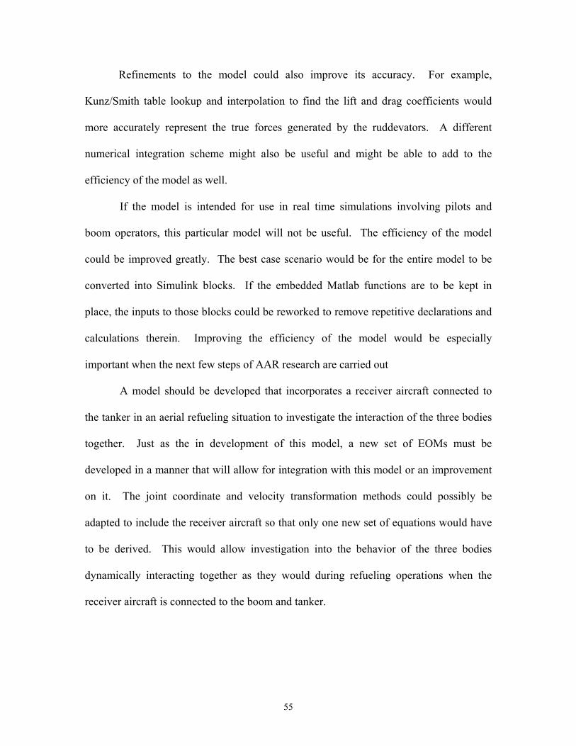
Refinements to the model could also improve its accuracy. For example,

Kunz/Smith table lookup and interpolation to find the lift and drag coefficients would

more accurately represent the true forces generated by the ruddevators. A different

numerical integration scheme might also be useful and might be able to add to the

efficiency of the model as well.

If the model is intended for use in real time simulations involving pilots and

boom operators, this particular model will not be useful. The efficiency of the model

could be improved greatly. The best case scenario would be for the entire model to be

converted into Simulink blocks. If the embedded Matlab functions are to be kept in

place, the inputs to those blocks could be reworked to remove repetitive declarations and

calculations therein. Improving the efficiency of the model would be especially

important when the next few steps of AAR research are carried out

A model should be developed that incorporates a receiver aircraft connected to

the tanker in an aerial refueling situation to investigate the interaction of the three bodies

together. Just as the in development of this model, a new set of EOMs must be

developed in a manner that will allow for integration with this model or an improvement

on it. The joint coordinate and velocity transformation methods could possibly be

adapted to include the receiver aircraft so that only one new set of equations would have

to be derived. This would allow investigation into the behavior of the three bodies

dynamically interacting together as they would during refueling operations when the

receiver aircraft is connected to the boom and tanker.

55

56

Appendix A

Vehicle ModelGeneralized Airframe Model Structure OUTPORT 1:

DATA TO FB FILTERSMach

Altitude_ftAlpha_degBeta_degRoll_deg

Pitch_degYaw_degPsens_dpsQsens_dpsRsens_dps

AXsens_fps2AYsens_fps2AZsens_fps2Airspeed_fps

qbar_psfPtotal_psfPstatic_psfwt_fuel_lb

wt_stores_lb

OUTPORT 2:MISC FLT DYN DATA

Pdot_dps2Qdot_dps2Rdot_dps2Udot_fps2Vdot_fps2Wdot_fps2

NL_gGamma_v_radAlpha_dot_rps

P_rpsQ_rpsR_rps

Clr_altitude_ft

OUTPORT 3:TSPI Data

North_ftEast_ft

Down_ft

OUTPORT 4: ATMOSPHERE

Tair_degRrho_slpft3

INPORT 1:Surf Commands In:

delPF_ddelElevonL_ddelElevonR_ddelClamL_ddelClamR_d

INPORT 2:PLA In:

PLA_deg

4Ext_Fb_Sigs

3atmos

2FDdata

1FBdata

alt

PQR

PQRdot

Fxy zB/m

FPAdat

Eulers

UVWdot

v t

aoa,beta

abdot

air data

atmos

load f act

PQRaero

clr_alt

PQR_sens

Axy z_sens

weights

Inertial_Pos

Boom_Pos

CL

VNED_f ps

FBdata

FDdata

Aero data

Atmos

Ext_Feedback_Sigs

Signal Router

Fbody

Mbody

Imat

mass

EXT

NED

Vned

qBtoG

latlon

grav

Rxy zI

Vxy zI

qBtoI

Axy zI

UVW

PQRw

alt

PQR

PQRdot

Fxy zB/m

FPAdat

Eulers

UVWdot

Vt

aoa,beta

abdot

air data

atmos

load f acts

PQRaero

clr alt

Rigid Body Motion

f f low

Inertias

ImatInv

mass_slug

weights

CGs

Mass Properties

CG_PQR

CG_PQRdot

Fxy zB/m

CG

sens_PQR

sens_Accels

IMU

Eulers

NED

Boom_NEA

Boom_Position_ft

Surf s Def ls

Aero Data

PLA

CGs

Eulers

FB

MB

Faero

Maero

f f low

CL

Aero and Propulsion Model

7

6

5

4

3

2

1

2

1

3EXT

2PLA

1Surf Cmds

Vt

<Eulers>

57

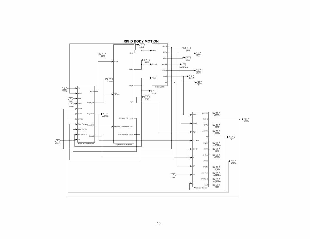
RIGID BODY MOTION

26clr alt

25PQRaero

24load facts

23atmos

22air data

21abdot

20aoa,beta

19Vt

18UVWdot

17Eulers

16FPAdat

15FxyzB/m

14PQRdot

13PQR

12alt

11PQRw

10UVW

9AxyzI

8qBtoI

7VxyzI

6RxyzI

5grav

4latlon

3qBtoG

2Vned

1NED

Terminator

Fb

qBtoI

IMat

Mass

Gxy zI

Eulers

atrmos

Joint Pos Vec

Joint Vel Vec

Vel_v ector_I

Mb

Axy zI

PQR_dot

Fxy zB/m

etadotdot

Gxy zB

Form Accelerations

qBtoI

Rxy zI

Vxy zI

Gxy zI

NED

latlon

alt_dot

qBtoG

Vned

alt

Flat_Earth

Axy zI

PQRdot

B Frame Acceleration v ec

qBtoI

Rxy zI

Vxy zI

PQR

B Frame Vel_v ector

B Frame Pos_v ector

Equations of Motion

Vned

qBtoG

PQR

Fxy zB/m

Gxy zB

alt

SPI

EXT

v t

gammas

Eulers

UVW

UVWdot

Vt

angles

abdot

air data

atmos

PQRw

Load Fact

PQRaero

clr_alt

Alternate States

5EXT

4mass

3Imat

2Mbody

1Fbody

58

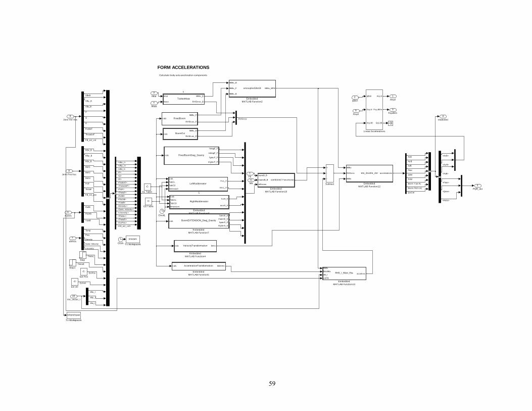
FORM ACCELERATIONSCalculate body axis acceleration components

4etadotdot

3FxyzB/m

2PQR_dot

1AxyzI

timesim

To Workspace6

rollpitchyaw

To Workspace5

Subtract

Step1

Step

qBtoI

Gxy zI

Axy zB

Axy zI

Fxy zB/m

Gxy zB

Linear Accelerations

-C-

Ext vel

-C-

Ext Pos

v als

TabCL

TabCD

timecount

f rv R_F

mrv R_F

RightRuddervator

EmbeddedMATLAB Function9

v als

f aeroE_E

maeroE_E

f grav E_E

mgrav E_E

BoomEXTENSION_Drag_Gravity

EmbeddedMATLAB Function7

v als bdotmtxAccelerationTransformation

EmbeddedMATLAB Function5

v als bmtxVelocityTransformation

EmbeddedMATLAB Function4

MMtx_B

MMtx_F

MMtx_E

MMtx_BFEuncoupled18x18

EmbeddedMATLAB Function2

MMtx

BdotMtx

VB_I

v elFB

accelv ecRHS_I_Bdot_Eta

EmbeddedMATLAB Function13

MMtx

RHSv ec

BMtx

accelerationseta_double_dot

EmbeddedMATLAB Function12

f aeroB_B

maeroB_B

allf orces

ForceVectorcombined

EmbeddedMATLAB Function10

Clock1

Clock

-C-

CL Table

-C-

CD Table

Imat

mass

MMtx_B

RHSIv ec_BTankerMass

1

v als

TabCL

TabCD

timecount

f rv L_F

mrv L_F

LeftRuddervator

1

v als

f dragF_F

mdragF_F

f grav F_F

mgrav F_F

FixedBoomDrag_Gravity

v als

MMtx_F

RHSIv ec_F

FixedBoom

v als

MMtx_E

RHSIv ec_EBoomExt

11Mb

10Vel_vector_I

9Joint Vel Vec

8Joint Pos Vec

7atrmos

6Eulers

5GxyzI

4Mass

3IMat 2

qBtoI

1Fb

AxB

Ay B

AzB

Pdot

Qdot

Rdot

Boom Pitch AC

<Ay B>

<AzB>

<AxB>

<Pdot>

<Qdot>

<Rdot>

VBxB

VBy _B

VBz_B

P

Q

R

PsidotF

ThetadotF

<VBx_I>

<VBy _I>

<VBz_I>

<P>

<Q>

<R>

RHSIv ec

<PsidotF>

<ThetadotF>

<PsiF>

<ThetaF>

<RollB>

<PitchB>

<YawB>

<Density >

<Sonic Velocity >

<v iscosity >

Boom Yaw Ac

ExtCtrl

<ThetaL>

<ThetaR>

<ExtPos>

<FB_ext_v el>

FB_ext_v el

RBx_B

RBy _B

RBz_B

blah1

blah2

blah3

PsiF

ThetaF

FB_ext_pos

RollB

PitchB

YawB

Temp

Pres

Density

Sonic Velocity

v iscosity

ThetaL

ThetaR

ExtPos

VBx_I

VBy _I

VBz_I

ExtVel

59

EQUATIONS OF MOTION

If the integration step is too large for the body rates, the quaternion can become denormalized and introduce attitude errors.

Stop the simulation if this is detected.Skip this on the first step since the quaternion may

not yet be normalized

OUTPORT 1OUTPUTS 1-3

INERTIAL POSITIONRxI_ftRyI_ftRzI_ft

OUTPORT 2OUTPUTS 4-6

INERTIAL VELOCITYVxI_fpsVyI_fpsVzI_fps

OUTPORT 3OUTPUTS 7-10QUATERNIONS

qBtoI0 qBtoI1 qBtoI2 qBtoI3

OUTPORT 4OUTPUTS 11-13

BODY RATESP_rpsQ_rpsR_rps

INPORT 1INPUTS 1-3

INERTIAL ACCELSAxI_fps2 AyI_fps2 AzI_fps2

INPORT 2

INPUTS 4-6ANGULAR ACCELS

Pdot_rps2Qdot_rps2Rdot_rps2

INPORT 3INPUTS 7-9

B Frame ACCELSAxB_fps2 AyB_fps2 AzB_fps2

6B Frame

Pos_vector

5B Frame

Vel_vector

4PQR

3VxyzI

2RxyzI

1qBtoI

pos_vec_I

To Workspace3

pos_vec_B

To Workspace2

vel_vec_B

To Workspace1

vel_vec_I

To Workspace

STOP

Stop Simulation>

RelationalOperator1

>

RelationalOperator

-K-

MagicTankerSwitch2

-K-

MagicTankerSwitch

AND

LogicalOperator

1s

Inertial Velocity

1s

Inertial Position

em

0

Constant1

.01

Constant

Clock

1s

Body Rates

1s

B Frame Velocity

1s

B Frame Position

PQR

qBtoI

norm_err

Attitude Quaternion

3B Frame

Acceleration vec

2PQRdot

1AxyzI

PQR_rps

R_rps

Q_rps

P_rps

60

61

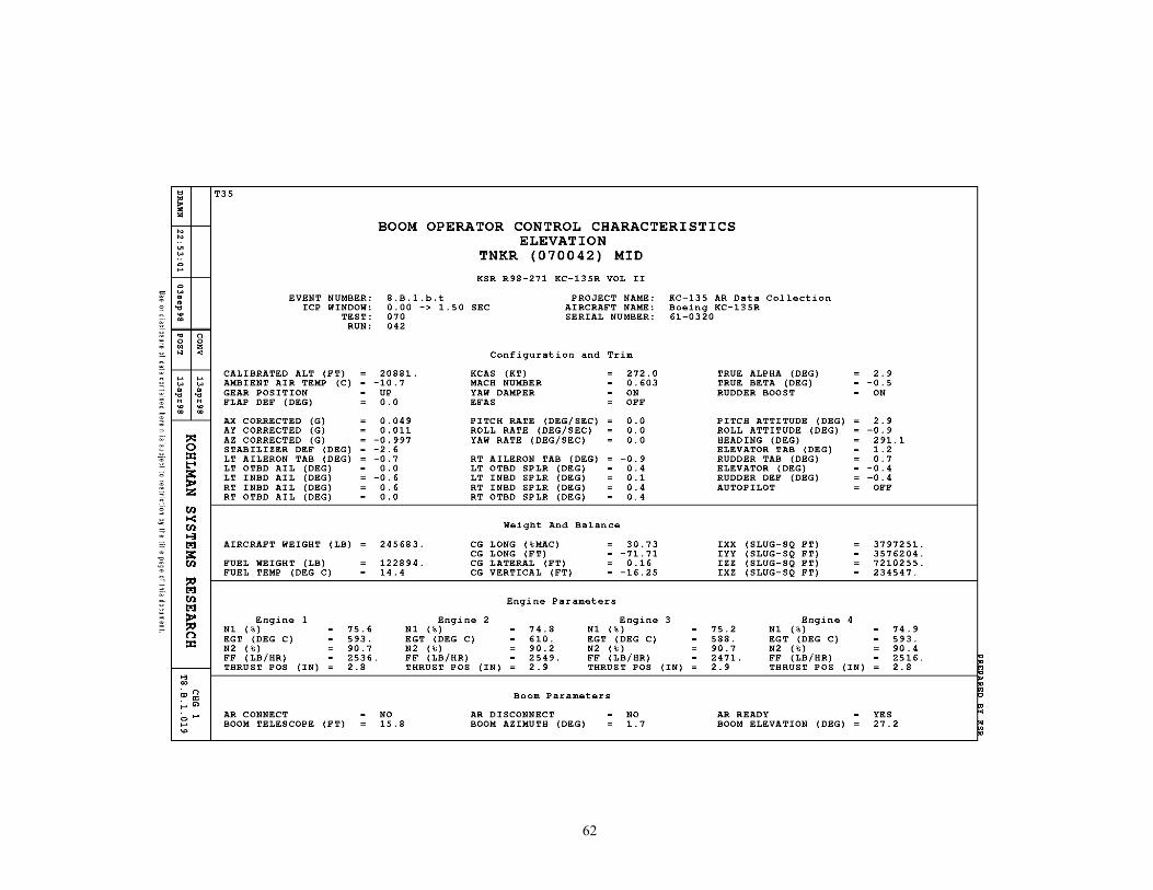
62

63

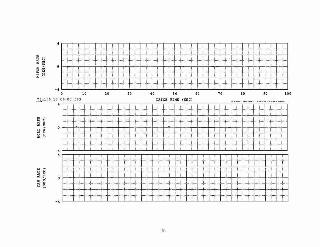
64

65

66

67

68

69

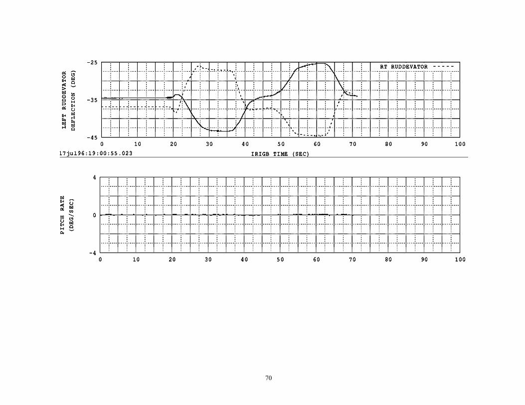
70

71

72

Appendix C

73

function [MMtx_B, RHSIvec_B] = TankerMass(Imat, mass) Zmx = zeros(3,3); MMtx = mass*eye(3); IMtx = [Imat(1), Imat(4), Imat(5);... Imat(4), Imat(2), Imat(6);... Imat(5), Imat(6), Imat(3)]; MMtx_B = [[MMtx], [Zmx]; [Zmx], [IMtx]]; % Extract values from the state vector omegaBI_B = zeros(3,1); omegaBI_B(1,1) = vals(4); omegaBI_B(2,1) = vals(5); omegaBI_B(3,1) = vals(6); % Right-hand side inertia vector Mvec = zeros( 3, 1 ); tildeB = [ 0, -omegaBI_B(3), omegaBI_B(2); ... omegaBI_B(3), 0, -omegaBI_B(1); ... -omegaBI_B(2), omegaBI_B(1), 0]; Ivec = tildeB*IMtx*omegaBI_B; RHSIvec_B = [ [Mvec]; . .. [Ivec]; ];

74

function [MMtx_F, RHSIvec_F] = FixedBoom(vals) ENVg_I = [0; 0; 32.174]; % Gravitational acceleration vector (ft/sec^2) % Fixed boom parameters FBOOML = 332/12; % fixed boom length (ft) FBOOMM = 756.5/norm( ENVg_I ); % slugs FBOOMrCG = [-228.88; 0; 0]/12; % fixed boom center of mass (ft) FBOOMIXX = 0.0; % slug-ft^2 FBOOMIYY = 3.294e5/norm( ENVg_I ); % slug-ft^2 FBOOMIZZ = 3.294e5/norm( ENVg_I ); % slug-ft^2 FBOOMIXY = 0.0; % slug-ft^2 FBOOMIXZ = 0.0; % slug-ft^2 FBOOMIYZ = 0.0; % slug-ft^2 FBOOMrFB_B = [583.325; 0; -12.5]/12; % fixed boom pivot location (ft) FBOOMnYaw_B = [0; 0; 1]; % Boom yaw axis (in the B basis) FBOOMnPitch_F = [0; 1; 0]; % Boom pitch axis (in the F basis) FBOOMDiam_in = [ 0.0, 240.0, 240.1, 332.0; ... 11.0, 11.0, 21.6, 21.6]; FBOOMrRF_F = [-294; 0; 0]/12; % ruddevator pivot location (ft) FBOOMRVc = 31/12; % ruddevator chord (ft) FBOOMRVL = 61/12; % ruddevator length (ft) FBOOMRVdihedral = 42*pi/180; % ruddevator dihedral angle (rad) Mmtx = FBOOMM*eye( 3 ); Rmtx = [0 0 0;0 0 0;0 0 0]; tildef = [ 0, -FBOOMrCG(3), FBOOMrCG(2); ... FBOOMrCG(3), 0, -FBOOMrCG(1); . .. -FBOOMrCG(2), FBOOMrCG(1), 0]; Rmtx = FBOOMM*tildef; Imtx = [ FBOOMIXX, FBOOMIXY, FBOOMIXZ; FBOOMIXY, FBOOMIYY, FBOOMIYZ; FBOOMIXZ, FBOOMIYZ, FBOOMIZZ ]; MMtx_F = [ [Mmtx], [-Rmtx]; ... [Rmtx], [Imtx] ]; %MMtx_F = zeros(6,6); % Extract values from the state vector omegaBI_B = zeros(3,1); omegaBI_B(1,1) = vals(4); omegaBI_B(2,1) = vals(5); omegaBI_B(3,1) = vals(6); YawFdot = vals(7); PitchFdot = vals(8); yawF = vals(9); pitchF = vals(10); roll = 0; % Define the direction cosine matrices dca = zeros( 3, 3 ); dca(1,1) = cos( yawF )*cos( pitchF ); dca(1,2) = sin( yawF )*cos( pitchF ); dca(1,3) = -sin( pitchF );

75

dca(2,1) = cos( yawF )*sin( pitchF )*sin( roll ) - sin( yawF )*cos( roll ); dca(2,2) = sin( yawF )*sin( pitchF )*sin( roll ) + cos( yawF )*cos( roll ); dca(2,3) = cos( pitchF )*sin( roll ); dca(3,1) = cos( yawF )*sin( pitchF )*cos( roll ) + sin( yawF )*sin( roll ); dca(3,2) = sin( yawF )*sin( pitchF )*cos( roll ) - cos( yawF )*sin( roll ); dca(3,3) = cos( pitchF )*cos( roll ); C_FB = dca; % Direction Cosine mx % Calculate the angular velocity omegaFB_F = C_FB*FBOOMnYaw_B*YawFdot + FBOOMnPitch_F*PitchFdot; omegaFI_F = omegaFB_F + C_FB*omegaBI_B; tildewFI_F = [ 0, -omegaFI_F(3), omegaFI_F(2); ... omegaFI_F(3), 0, -omegaFI_F(1); ... -omegaFI_F(2), omegaFI_F(1), 0]; % Right-hand side inertia vector Mvec = FBOOMM*tildewFI_F*tildewFI_F*FBOOMrCG; Ivec = tildewFI_F*Imtx*omegaFI_F; RHSIvec_F = [ [Mvec]; ... [Ivec]; ]; %RHSIvec_F = zeros(6,1);

76

function [MMtx_E, RHSIvec_E] = BoomExt(vals) % % Construct the mass/inertia matrix and the right-hand side inertia vector for the boom extension %---------------------------------------- % Extract values from state vector uE = vals(19); % Extension is controlled % Boom extension parameters EBOOML = 330/12; % boom extension length (ft) EBOOMM = 460.35/32.2; % slugs EBOOMrCG = [-178.84; 0; 0]/12; % boom extension center of mass (ft) EBOOMIXX = 0.0; % slug-ft^2 EBOOMIYY = 1.414e5/32.2; % slug-ft^2 EBOOMIZZ = 1.414e5/32.2; % [slug-ft^2 EBOOMIXY = 0.0; % slug-ft^2 EBOOMIXZ = 0.0; % slug-ft^2 EBOOMIYZ = 0.0; % slug-ft^2 EBOOMnExt_E = [1; 0; 0]; % Boom extension axis (in the E basis) EBOOMrEF_F = [-2; 0; 0]/12; % Stowed extension position (in the F basis) EBOOMD = 3.1*2/12; % boom extension diameter (ft) FBOOMrFB_B = [583.325; 0; -12.5]/12; % fixed boom pivot location (ft) FBOOMnYaw_B = [0; 0; 1]; % Boom yaw axis (in the B basis) FBOOMnPitch_F = [0; 1; 0]; % Boom pitch axis (in the F basis) % Contributions from fuel during extension fuel = 0.14546; fuel distributed mass (slug/ft) %fmass = fuel*uE; % Combined boom extension mass mass = EBOOMM + fmass; % Combined boom extension center of mass rCG = (EBOOMM*EBOOMrCG + fmass*[uE/2; 0; 0])/mass; % Combined boom extension moments of inertia IYY = EBOOMIYY + (fmass*(uE/2)^2)/3; IZZ = EBOOMIZZ + (fmass*(uE/2)^2)/3; % Construct the mass/inertia matrix in the stowed position Mmtx = mass*eye( 3 ); Rmtx = [0 0 0;0 0 0;0 0 0]; tildee = [ 0, -rCG(3), rCG(2); ... rCG(3), 0, -rCG(1); ... -rCG(2), rCG(1), 0]; Rmtx = EBOOMM*tildee; Imtx = [ EBOOMIXX, EBOOMIXY, EBOOMIXZ; EBOOMIXY, IYY, EBOOMIYZ; EBOOMIXZ, EBOOMIYZ, IZZ ]; MMtx_E = [ [Mmtx], [-Rmtx]; ... [Rmtx], [Imtx] ];

77

%MMtx_E = zeros(6,6); % Extract values from the state vector omegaBI_B = zeros(3,1); omegaBI_B(1,1) = vals(4); omegaBI_B(2,1) = vals(5); omegaBI_B(3,1) = vals(6); YawFdot = vals(7); PitchFdot = vals(8); yawF = vals(9); pitchF = vals(10); roll = 0; % Define the direction cosine matrices dca = zeros( 3, 3 ); dca(1,1) = cos( yawF )*cos( pitchF ); dca(1,2) = sin( yawF )*cos( pitchF ); dca(1,3) = -sin( pitchF ); dca(2,1) = cos( yawF )*sin( pitchF )*sin( roll ) - sin( yawF )*cos( roll ); dca(2,2) = sin( yawF )*sin( pitchF )*sin( roll ) + cos( yawF )*cos( roll ); dca(2,3) = cos( pitchF )*sin( roll ); dca(3,1) = cos( yawF )*sin( pitchF )*cos( roll ) + sin( yawF )*sin( roll ); dca(3,2) = sin( yawF )*sin( pitchF )*cos( roll ) - cos( yawF )*sin( roll ); dca(3,3) = cos( pitchF )*cos( roll ); C_FB = dca; % Direction Cosine mx C_EF = eye( 3 ); C_EB = C_EF*C_FB; % Calculate the angular velocity omegaEF_E = zeros( 3, 1 ); omegaFB_F = C_FB*FBOOMnYaw_B*YawFdot + FBOOMnPitch_F*PitchFdot; omegaEI_E = omegaEF_E + C_EF*omegaFB_F + C_EB*omegaBI_B; tildewEI_E = [ 0, -omegaEI_E(3), omegaEI_E(2); ... omegaEI_E(3), 0, -omegaEI_E(1); ... -omegaEI_E(2), omegaEI_E(1), 0]; % Right-hand side inertia vector Mvec = mass*tildewEI_E*tildewEI_E*rCG; Ivec = tildewEI_E*Imtx*omegaEI_E; RHSIvec_E = [ [Mvec]; . .. [Ivec]; ]; %RHSIvec_E = zeros(6,1);

78

function [fdragF_F, mdragF_F, fgravF_F, mgravF_F ] = FixedBoomDrag_Gravity(vals) % % Calculate the drag/gravity forces/moments on the fixed boom. % %---------------------------------------- % Extract values from the state vector %Tanker Velocity in the I frame vBI_I = zeros(3,1); vBI_I(1,1) = vals(1); vBI_I(2,1) = vals(2); vBI_I(3,1) = vals(3); %Tanker angular velocity in the B frame omegaBI_B = zeros(3,1); omegaBI_B(1,1) = vals(4); omegaBI_B(2,1) = vals(5); omegaBI_B(3,1) = vals(6); % Tanker Euler Angles yawB = vals(13); pitchB = vals(12) ;rollB = vals(11); % Fixed Boom angular Rates YawFdot = vals(7); PitchFdot = vals(8); % Fixed Boom Attitude yawF = vals(9); pitchF = vals(10); rollF = 0; % Atmosperic data ENVrho = vals(14); % density; % Air density at sea level (slug/ft^3) ENVa = vals(15); %vsound; % Speed of sound (ft/sec) % visc from the original AFRL program does not update (comes in as 0) ENVvisc = 3.21596084e-7; % vals(16); %visc; % Viscosity (lbf-sec/ft^2) ENVg_I = [0; 0; 32.174]; % Gravitational acceleration vector (ft/sec^2) FBOOMnYaw_B = [0; 0; 1]; % Boom yaw axis (in the B basis) FBOOMnPitch_F = [0; 1; 0]; % Boom pitch axis (in the F basis) FBOOMrFB_B = [583.325; 0; -12.5]/12; % fixed boom pivot location (ft) FBOOML = 332/12; % fixed boom length (ft) FBOOMM = 756.5/32.2; % slugs FBOOMrCG = [-228.88; 0; 0]/12; % fixed boom center of mass (ft) FBOOMDiam_in = [ 0.0, 240.0, 240.1, 332.0; ... 11.0, 11.0, 21.6, 21.6]; % Define the direction cosine matrices dca = zeros( 3, 3 ); dca(1,1) = cos( yawB )*cos( pitchB ); dca(1,2) = sin( yawB )*cos( pitchB ); dca(1,3) = -sin( pitchB ); dca(2,1) = cos( yawB )*sin( pitchB )*sin( rollB ) - sin( yawB )*cos( rollB ); dca(2,2) = sin( yawB )*sin( pitchB )*sin( rollB ) + cos( yawB )*cos( rollB ); dca(2,3) = cos( pitchB )*sin( rollB ); dca(3,1) = cos( yawB )*sin( pitchB )*cos( rollB ) + sin( yawB )*sin( rollB );

79

dca(3,2) = sin( yawB )*sin( pitchB )*cos( rollB ) - cos( yawB )*sin( rollB ); dca(3,3) = cos( pitchB )*cos( rollB ); C_BI = dca; dca = zeros( 3, 3 ); dca(1,1) = cos( yawF )*cos( pitchF ); dca(1,2) = sin( yawF )*cos( pitchF ); dca(1,3) = -sin( pitchF ); dca(2,1) = cos( yawF )*sin( pitchF )*sin( rollF ) - sin( yawF )*cos( rollF ); dca(2,2) = sin( yawF )*sin( pitchF )*sin( rollF ) + cos( yawF )*cos( rollF ); dca(2,3) = cos( pitchF )*sin( rollF ); dca(3,1) = cos( yawF )*sin( pitchF )*cos( rollF ) + sin( yawF )*sin( rollF ); dca(3,2) = sin( yawF )*sin( pitchF )*cos( rollF ) - cos( yawF )*sin( rollF ); dca(3,3) = cos( pitchF )*cos( rollF ); C_FB = dca; C_FI = C_FB*C_BI; % Define the velocities and angular velocities vBI_B = C_BI*vBI_I; omegaFB_F = C_FB*FBOOMnYaw_B*YawFdot + FBOOMnPitch_F*PitchFdot; omegaFI_F = omegaFB_F + C_FB*omegaBI_B; x0 = FBOOML; x1 = 0; x = linspace(-x0, x1); vpI_F = [0;0;0]; tildeFBOOMrFB_B = [ 0, -FBOOMrFB_B(3), FBOOMrFB_B(2); ... FBOOMrFB_B(3), 0, -FBOOMrFB_B(1); ... -FBOOMrFB_B(2), FBOOMrFB_B(1), 0]; dragY = zeros(1,length(x)); dragZ = zeros(1,length(x)); momentY = zeros(1,length(x)); momentZ = zeros(1,length(x)); for j = 1:1:length(x) tilderpF_F = [ 0, -0, 0; ... 0, 0, -x(j); ... -0, x(j), 0]; vpI_F = C_FB*(vBI_B - tildeFBOOMrFB_B*omegaBI_B) ... - tilderpF_F*omegaFI_F; Vy = vpI_F(2); Vz = vpI_F(3); V = sqrt( Vy^2 + Vz^2); % Calculate the cross section drag coefficient if( V > 1.0e-5 ) diam = interp1( FBOOMDiam_in(1,:)/12, FBOOMDiam_in(2,:)/12, -x(j) ); Re = ENVrho*V*diam/ENVvisc; if( Re <= 1 )

80

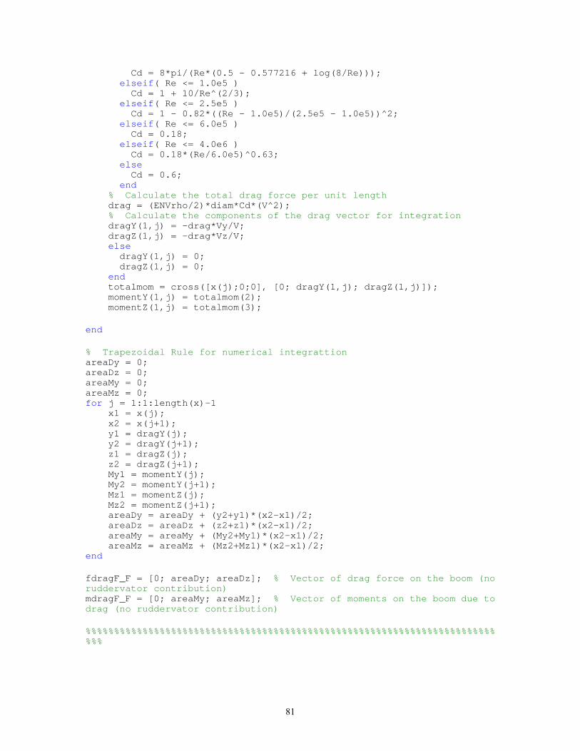
Cd = 8*pi/(Re*(0.5 - 0.577216 + log(8/Re))); elseif( Re <= 1.0e5 ) Cd = 1 + 10/Re^(2/3); elseif( Re <= 2.5e5 ) Cd = 1 - 0.82*((Re - 1.0e5)/(2.5e5 - 1.0e5))^2; elseif( Re <= 6.0e5 ) Cd = 0.18; elseif( Re <= 4.0e6 ) Cd = 0.18*(Re/6.0e5)^0.63; else Cd = 0.6; end % Calculate the total drag force per unit length drag = (ENVrho/2)*diam*Cd*(V^2); % Calculate the components of the drag vector for integration dragY(1,j) = -drag*Vy/V; dragZ(1,j) = -drag*Vz/V; else dragY(1,j) = 0; dragZ(1,j) = 0; end totalmom = cross([x(j);0;0], [0; dragY(1,j); dragZ(1,j)]); momentY(1,j) = totalmom(2); momentZ(1,j) = totalmom(3); end % Trapezoidal Rule for numerical integrattion areaDy = 0; areaDz = 0; areaMy = 0; areaMz = 0; for j = 1:1:length(x)-1 x1 = x(j); x2 = x(j+1); y1 = dragY(j); y2 = dragY(j+1); z1 = dragZ(j); z2 = dragZ(j+1); My1 = momentY(j); My2 = momentY(j+1); Mz1 = momentZ(j); Mz2 = momentZ(j+1); areaDy = areaDy + (y2+y1)*(x2-x1)/2; areaDz = areaDz + (z2+z1)*(x2-x1)/2; areaMy = areaMy + (My2+My1)*(x2-x1)/2; areaMz = areaMz + (Mz2+Mz1)*(x2-x1)/2; end fdragF_F = [0; areaDy; areaDz]; % Vector of drag force on the boom (no ruddervator contribution) mdragF_F = [0; areaMy; areaMz]; % Vector of moments on the boom due to drag (no ruddervator contribution) %%%%%%%%%%%%%%%%%%%%%%%%%%%%%%%%%%%%%%%%%%%%%%%%%%%%%%%%%%%%%%%%%%%%%%%%%%%

81

% GRAVITY VECTOR CALCULATIONS FOR THE FIXED BOOM % %%%%%%%%%%%%%%%%%%%%%%%%%%%%%%%%%%%%%%%%%%%%%%%%%%%%%%%%%%%%%%%%%%%%%%%%%%% % Define the gravitational vector gVec_F = C_FI*ENVg_I; % Calculate the force acting at the boom pivot (F) fgravF_F = FBOOMM*gVec_F; % Calculate the moment acting about the boom pivot (F) rCF_F = FBOOMrCG; mgravF_F = cross( rCF_F, fgravF_F );

82

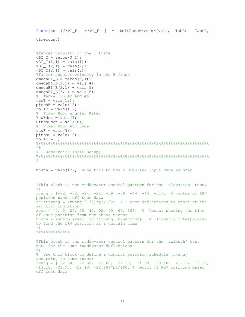
function [frvL_F, mrvL_F ] = LeftRuddervator(vals, TabCL, TabCD,

timecount)

%Tanker Velocity in the I frame vBI_I = zeros(3,1); vBI_I(1,1) = vals(1); vBI_I(2,1) = vals(2); vBI_I(3,1) = vals(3); %Tanker angular velocity in the B frame omegaBI_B = zeros(3,1); omegaBI_B(1,1) = vals(4); omegaBI_B(2,1) = vals(5); omegaBI_B(3,1) = vals(6); % Tanker Euler Angles yawB = vals(13); pitchB = vals(12) ;rollB = vals(11); % Fixed Boom angular Rates YawFdot = vals(7); PitchFdot = vals(8); % Fixed Boom Attitude yawF = vals(9); pitchF = vals(10); rollF = 0; %%%%%%%%%%%%%%%%%%%%%%%%%%%%%%%%%%%%%%%%%%%%%%%%%%%%%%%%%%%%%%%%%%%%%%%%%% % Ruddervator Angle Setup; %%%%%%%%%%%%%%%%%%%%%%%%%%%%%%%%%%%%%%%%%%%%%%%%%%%%%%%%%%%%%%%%%%%%%%%%% theta = vals(17); %Use this to use a Simulink input such as step %This block is the ruddevator control pattern for the 'elevation' test. %{ rvang = [-32, -32, -24, -24, -39, -39, -44, -44, -31]; % vector of LRV position based off test data shiftrvang = (rvang+9.32)*pi/180; % Force deflections to start at the sim trim condition xvec = [0, 5, 20, 30, 45, 52, 60, 67, 80]; % Vector showing the time of each position from the above vector theta = interp1(xvec, shiftrvang, timecount); % linearly interpolates to find the LRV position at a certain time %} %%%%%%%%%%%%%% %This block is the ruddevator control pattern for the 'azimuth' test data for the same ruddevator deflections %{ % Use this block to define a control position schedule (rvang) according to time (xvec) rvang = [-22.68, -22.68, -21.68, -31.68, -31.68, -23.18, -21.18, -15.18, -13.18, -21.93, -22.18, -22.18]*pi/180; % vector of RRV position based off test data

83

xvec = [0, 20, 21.25, 28, 37, 42.5, 49, 54, 62.5, 68, 75, 80 ]; % Vector showing the time of each position from the above vector theta = interp1(xvec, rvang, timecount); % linearly interpolates to find the LRV position at a certain time %%%%%%%%%%%%%%% %} %%%%%%%%%%%%%%%%%%%%%%%%%%%%%%%%%%%%%%%%%%%%%%%%%%%%%%%%%%%%%%%%%%%%%%%%%%%% % Atmosperic data ENVrho = vals(14); % density; % Air density at sea level (slug/ft^3) ENVa = vals(15); %vsound; % Speed of sound (ft/sec) ENVvisc = vals(16); %visc; % Viscosity (lbf-sec/ft^2) ENVg_I = [0; 0; 32.174]; % Gravitational acceleration vector (ft/sec^2) FBOOMnYaw_B = [0; 0; 1]; % Boom yaw axis (in the B basis) FBOOMnPitch_F = [0; 1; 0]; % Boom pitch axis (in the F basis) FBOOMrFB_B = [583.325; 0; -12.5]/12; % fixed boom pivot location (ft) FBOOML = 332/12; % fixed boom length (ft) FBOOMM = 756.5/32.2; % slugs FBOOMrCG = [-228.88; 0; 0]/12; % fixed boom center of mass (ft) FBOOMDiam_in = [ 0.0, 240.0, 240.1, 332.0; ... 11.0, 11.0, 21.6, 21.6]; FBOOMrRF_F = [-294; 0; 0]/12; % ruddevator pivot location (ft) FBOOMRVc = 31/12; % ruddevator chord (ft) FBOOMRVL = 61/12; % ruddevator length (ft) FBOOMRVdihedral = 42*pi/180; % ruddevator dihedral angle (rad) FBOOMRVTabCL = TabCL; FBOOMRVTabCD = TabCD; FBOOMRVCtrl = 0; %boomCtrl(:,1:3); % ruddevator control angles (deg) % Define the direction cosine matrices dca = zeros( 3, 3 ); dca(1,1) = cos( yawB )*cos( pitchB ); dca(1,2) = sin( yawB )*cos( pitchB ); dca(1,3) = -sin( pitchB ); dca(2,1) = cos( yawB )*sin( pitchB )*sin( rollB ) - sin( yawB )*cos( rollB ); dca(2,2) = sin( yawB )*sin( pitchB )*sin( rollB ) + cos( yawB )*cos( rollB ); dca(2,3) = cos( pitchB )*sin( rollB ); dca(3,1) = cos( yawB )*sin( pitchB )*cos( rollB ) + sin( yawB )*sin( rollB ); dca(3,2) = sin( yawB )*sin( pitchB )*cos( rollB ) - cos( yawB )*sin( rollB ); dca(3,3) = cos( pitchB )*cos( rollB ); C_BI = dca; dca = zeros( 3, 3 ); dca(1,1) = cos( yawF )*cos( pitchF ); dca(1,2) = sin( yawF )*cos( pitchF ); dca(1,3) = -sin( pitchF ); dca(2,1) = cos( yawF )*sin( pitchF )*sin( rollF ) - sin( yawF )*cos( rollF );

84

dca(2,2) = sin( yawF )*sin( pitchF )*sin( rollF ) + cos( yawF )*cos( rollF ); dca(2,3) = cos( pitchF )*sin( rollF ); dca(3,1) = cos( yawF )*sin( pitchF )*cos( rollF ) + sin( yawF )*sin( rollF ); dca(3,2) = sin( yawF )*sin( pitchF )*cos( rollF ) - cos( yawF )*sin( rollF ); dca(3,3) = cos( pitchF )*cos( rollF ); C_FB = dca; C_FI = C_FB*C_BI; % Define the velocities and angular velocities vBI_B = C_BI*vBI_I; omegaFB_F = C_FB*FBOOMnYaw_B*YawFdot + FBOOMnPitch_F*PitchFdot; omegaFI_F = omegaFB_F + C_FB*omegaBI_B; %%%%%%%%%%%%%%%%%%%%%%%%%%%%%%%%%%%%%%%%%%%%%%%%%%%%%%%%%%%%%%%%%%%%%%%%%%% % FORCE VECTOR CALCULATIONS FOR THE RUDDERVATORS % %%%%%%%%%%%%%%%%%%%%%%%%%%%%%%%%%%%%%%%%%%%%%%%%%%%%%%%%%%%%%%%%%%%%%%%%%%% %%%%%%%%%%%%%%%%%%%%%%%%%%%%%%%%%%%%%%%%%%%%%%%%%%%%%%%%%%%%%%%% % Left Ruddervator % %%%%%%%%%%%%%%%%%%%%%%%%%%%%%%%%%%%%%%%%%%%%%%%%%%%%%%%%%%%%%%%% yaw = 0; pitch = 0; roll = FBOOMRVdihedral; dca = zeros( 3, 3 ); dca(1,1) = cos( yaw )*cos( pitch ); dca(1,2) = sin( yaw )*cos( pitch ); dca(1,3) = -sin( pitch ); dca(2,1) = cos( yaw )*sin( pitch )*sin( roll ) - sin( yaw )*cos( roll ); dca(2,2) = sin( yaw )*sin( pitch )*sin( roll ) + cos( yaw )*cos( roll ); dca(2,3) = cos( pitch )*sin( roll ); dca(3,1) = cos( yaw )*sin( pitch )*cos( roll ) + sin( yaw )*sin( roll ); dca(3,2) = sin( yaw )*sin( pitch )*cos( roll ) - cos( yaw )*sin( roll ); dca(3,3) = cos( pitch )*cos( roll ); C_WF = dca; C_WB = C_WF*C_FB; C_FW = C_WF'; y0 = -FBOOMRVL; y1 = -interp1( FBOOMDiam_in(1,:)/12, FBOOMDiam_in(2,:)/12, ... -FBOOMrRF_F(1) )/2; y = linspace(y0, y1); % Integration limits tildeFBOOMrFB_B = [ 0, -FBOOMrFB_B(3), FBOOMrFB_B(2); ... FBOOMrFB_B(3), 0, -FBOOMrFB_B(1); ... -FBOOMrFB_B(2), FBOOMrFB_B(1), 0]; C_WZ = zeros(3,3); df_W = zeros(3,1); df_Wx = zeros(1, length(y)); df_Wz = zeros(1, length(y));

85

dm_Wx = zeros(1, length(y)); dm_Wz = zeros(1, length(y)); AoAvecCL = [TabCL(2:40, 1)]; AoAvecCD = [TabCD(2:56, 1)]; for j = 1:1:length(y) rpF_F = FBOOMrRF_F + C_FW*[0;y(j);0 tilderpF_F = [ 0, -rpF_F(3), rpF_F(2); ... rpF_F(3), 0, -rpF_F(1); ... -rpF_F(2), rpF_F(1), 0]; vpI_W = C_WB*(vBI_B - tildeFBOOMrFB_B*omegaBI_B) ... - C_WF*tilderpF_F*omegaFI_F; V = vpI_W; VxVy = sign( V(1) )*sqrt( V(1)^2 + V(2)^2 ); SweepFactor = abs( V(1)/VxVy ); phi = atan2( V(3), VxVy ); AoA = atan2( SweepFactor*sin( theta ), cos( theta ) ) + phi; shiftAoA = (abs( AoA ) > pi)*sign( AoA )*(2*pi); AoA = AoA - shiftAoA; AoAdeg = AoA*180/pi; % Calculate the section Mach number Vnorm = norm( V ); Mach = abs( Vnorm/ENVa ); % Interpolate from the C81 tables (this is where the 2D interpolation fn was moved to one. Can’t use interp2 in an embedded fn CLvec = zeros(39,1); CDvec = zeros(55,1); if Mach >0 & Mach <= .1 CLvec = [TabCL(2:40, 2)]; CDvec = [TabCD(2:56, 2)]; elseif Mach >.1 && Mach <= .25 CLvec = [TabCL(2:40, 3)]; CDvec = [TabCD(2:56, 3)]; elseif Mach >.25 && Mach <= .35 CLvec = [TabCL(2:40, 4)]; CDvec = [TabCD(2:56, 4)]; elseif Mach >.35 && Mach <= .45 CLvec = [TabCL(2:40, 5)]; CDvec = [TabCD(2:56, 5)]; elseif Mach >.45 && Mach <= .55 CLvec = [TabCL(2:40, 6)]; CDvec = [TabCD(2:56, 6)]; elseif Mach >.55 && Mach <= . 8 CLvec = [TabCL(2:40, 7)]; CDvec = [TabCD(2:56, 7)]; elseif Mach >.8 && Mach <= 1 CLvec = [TabCL(2:40, 8)]; CDvec = [TabCD(2:56, 8)]; end k0 = CLvec; g0 = CDvec; CL = interp1(AoAvecCL, k0, AoAdeg); CD = interp1(AoAvecCD, g0, AoAdeg);

86

% Calculate the section forces df_Zx = (ENVrho/2)*(Vnorm^2)*FBOOMRVc*CD; df_Zz = (ENVrho/2)*(Vnorm^2)*FBOOMRVc*CL; yaw = 0; roll = 0; pitch = pi - phi; dca = zeros( 3, 3 ); dca(1,1) = cos( yaw )*cos( pitch ); dca(1,2) = sin( yaw )*cos( pitch ); dca(1,3) = -sin( pitch ); dca(2,1) = cos( yaw )*sin( pitch )*sin( roll ) - sin( yaw )*cos( roll ); dca(2,2) = sin( yaw )*sin( pitch )*sin( roll ) + cos( yaw )*cos( roll ); dca(2,3) = cos( pitch )*sin( roll ); dca(3,1) = cos( yaw )*sin( pitch )*cos( roll ) + sin( yaw )*sin( roll ); dca(3,2) = sin( yaw )*sin( pitch )*cos( roll ) - cos( yaw )*sin( roll ); dca(3,3) = cos( pitch )*cos( roll ); C_WZ = dca; df_W = C_WZ*[df_Zx;0;df_Zz]; df_Wx(1,j) = df_W(1); % vector of differential forces to integrate df_Wz(1,j) = df_W(3); % vector of differential forces to integrate totalmom = cross([0; y(j); 0], [df_Wx(1,j); 0; df_Wz(1,j)]); dm_Wx(1,j) = totalmom(1); % vector of differential moments to integrate dm_Wz(1,j) = totalmom(3); % vector of differential moments to integrate end % Trapezoidal Rule for numerical integrattion areaDx = 0; areaDz = 0; areaMx = 0; areaMz = 0; for j = 1:1:length(y)-1 x1 = y(j); x2 = y(j+1); y1 = df_Wx(j); y2 = df_Wx(j+1); z1 = df_Wz(j); z2 = df_Wz(j+1) ; Mx1 = dm_Wx(j); Mx2 = dm_Wx(j+1); Mz1 = dm_Wz(j); Mz2 = dm_Wz(j+1); areaDx = areaDx + (y2+y1)*(x2-x1)/2; areaDz = areaDz + (z2+z1)*(x2-x1)/2; areaMx = areaMx + (Mx2+Mx1)*(x2-x1)/2; areaMz = areaMz + (Mz2+Mz1)*(x2-x1)/2; end

87

frvW_W = [areaDx; 0; areaDz]; % Vector of force on the LEFT ruddervator (in the W basis) mrvW_W = [areaMx; 0; areaMz]; % Vector of moments on the LEFT ruddervator (in the W basis) frvL_F = C_FW*frvW_W; % Vector of force on the LEFT ruddervator (in the F basis) mrvL_F = C_FW*mrvW_W; % Vector of moments on the LEFT ruddervator (in the F basis)

88

function [frvR_F, mrvR_F ] = RightRuddervator( vals, TabCL, TabCD, timecount) % % Calculate the force/moment contribution of the right RV % %---------------------------------------- %Tanker Velocity in the I frame vBI_I = zeros(3,1); vBI_I(1,1) = vals(1); vBI_I(2,1) = vals(2); vBI_I(3,1) = vals(3); %Tanker angular velocity in the B frame omegaBI_B = zeros(3,1); omegaBI_B(1,1) = vals(4); omegaBI_B(2,1) = vals(5); omegaBI_B(3,1) = vals(6); % Tanker Euler Angles yawB = vals(13); pitchB = vals(12); rollB = vals(11); % Fixed Boom angular Rates YawFdot = vals(7); PitchFdot = vals(8); % Fixed Boom Attitude yawF = vals(9); pitchF = vals(10); rollF = 0; % Ruddervator Angle; theta = vals(18); % Use this if you want to use a step or ramp input %%%%%%%%% % Ruddervator Angle; Use this for the flight test data % This block is the ruddevator control pattern for the 'elevation' test data for the same ruddevator deflections %{ rvang = [-32, -32, -24, -24, -39, -39, -44, -44, -31]; % vector of RRV position based off test data shiftrvang = (rvang+9.32)*pi/180; % Force deflections to start at the trim condition xvec = [0, 5, 20, 30, 45, 52, 60, 67, 80]; % Vector showing the time of each position from the above vector theta = interp1(xvec, shiftrvang, timecount); % linearly interpolates to find the RRV position at a certain time %%%%%%%%%%%%%%%% %} %This block is the ruddevator control pattern for the 'azimuth' test data for the same ruddevator deflections %{ rvang = [-22.68, -22.68, -23.68, -14.68, -14.68, -22.68, -24.18, -29.18, -31.43, -22.43, -22.18, -22.18]*pi/180; % vector of RRV position based off test data xvec = [0, 20, 21.25, 28, 37, 42.5, 49, 54, 62.5, 68, 75, 80, ]; % Vector showing the time of each position from the above vector

89

theta = interp1(xvec, rvang, timecount); % linearly interpolates to find the RRV position at a certain time %} %%%%%%%%%%%%%%%%%%% % Atmosperic data ENVrho = vals(14); % density; % Air density at sea level (slug/ft^3) ENVa = vals(15); %vsound; % Speed of sound (ft/sec) ENVvisc = vals(16); %visc; % Viscosity (lbf-sec/ft^2) ENVg_I = [0; 0; 32.174]; % Gravitational acceleration vector (ft/sec^2) FBOOMnYaw_B = [0; 0; 1]; % Boom yaw axis (in the B basis) FBOOMnPitch_F = [0; 1; 0]; % Boom pitch axis (in the F basis) FBOOMrFB_B = [583.325; 0; -12.5]/12; % fixed boom pivot location (ft) FBOOML = 332/12; % fixed boom length (ft) FBOOMM = 756.5/32.2; % slugs FBOOMrCG = [-228.88; 0; 0]/12; % fixed boom center of mass (ft) FBOOMDiam_in = [ 0.0, 240.0, 240.1, 332.0; ... 11.0, 11.0, 21.6, 21.6]; FBOOMrRF_F = [-294; 0; 0]/12; % ruddevator pivot location (ft) FBOOMRVc = 31/12; % ruddevator chord (ft) FBOOMRVL = 61/12; % ruddevator length (ft) FBOOMRVdihedral = 42*pi/180; % ruddevator dihedral angle (rad) FBOOMRVTabCL = TabCL; FBOOMRVTabCD = TabCD; FBOOMRVCtrl = 0; %boomCtrl(:,1:3); % ruddevator control angles (deg) % Define the direction cosine matrices dca = zeros( 3, 3 ); dca(1,1) = cos( yawB )*cos( pitchB ); dca(1,2) = sin( yawB )*cos( pitchB ); dca(1,3) = -sin( pitchB ); dca(2,1) = cos( yawB )*sin( pitchB )*sin( rollB ) - sin( yawB )*cos( rollB ); dca(2,2) = sin( yawB )*sin( pitchB )*sin( rollB ) + cos( yawB )*cos( rollB ); dca(2,3) = cos( pitchB )*sin( rollB ); dca(3,1) = cos( yawB )*sin( pitchB )*cos( rollB ) + sin( yawB )*sin( rollB ); dca(3,2) = sin( yawB )*sin( pitchB )*cos( rollB ) - cos( yawB )*sin( rollB ); dca(3,3) = cos( pitchB )*cos( rollB ); C_BI = dca; dca = zeros( 3, 3 ); dca(1,1) = cos( yawF )*cos( pitchF ); dca(1,2) = sin( yawF )*cos( pitchF ); dca(1,3) = -sin( pitchF ); dca(2,1) = cos( yawF )*sin( pitchF )*sin( rollF ) - sin( yawF )*cos( rollF ); dca(2,2) = sin( yawF )*sin( pitchF )*sin( rollF ) + cos( yawF )*cos( rollF ); dca(2,3) = cos( pitchF )*sin( rollF ); dca(3,1) = cos( yawF )*sin( pitchF )*cos( rollF ) + sin( yawF )*sin( rollF );

90

dca(3,2) = sin( yawF )*sin( pitchF )*cos( rollF ) - cos( yawF )*sin( rollF ); dca(3,3) = cos( pitchF )*cos( rollF ); C_FB = dca; C_FI = C_FB*C_BI; % Define the velocities and angular velocities vBI_B = C_BI*vBI_I; omegaFB_F = C_FB*FBOOMnYaw_B*YawFdot + FBOOMnPitch_F*PitchFdot; omegaFI_F = omegaFB_F + C_FB*omegaBI_B; %%%%%%%%%%%%%%%%%%%%%%%%%%%%%%%%%%%%%%%%%%%%%%%%%%%%%%%%%%%%%%%%%%%%%%%%%%% % FORCE VECTOR CALCULATIONS FOR THE RUDDERVATORS % %%%%%%%%%%%%%%%%%%%%%%%%%%%%%%%%%%%%%%%%%%%%%%%%%%%%%%%%%%%%%%%%%%%%%%%%%%% %%%%%%%%%%%%%%%%%%%%%%%%%%%%%%%%%%%%%%%%%%%%%%%%%%%%%%%%%%%%%%%% % Right Ruddervator % %%%%%%%%%%%%%%%%%%%%%%%%%%%%%%%%%%%%%%%%%%%%%%%%%%%%%%%%%%%%%%%% yaw = 0; pitch = 0; roll = -FBOOMRVdihedral; dca = zeros( 3, 3 ); dca(1,1) = cos( yaw )*cos( pitch ); dca(1,2) = sin( yaw )*cos( pitch ); dca(1,3) = -sin( pitch ); dca(2,1) = cos( yaw )*sin( pitch )*sin( roll ) - sin( yaw )*cos( roll ); dca(2,2) = sin( yaw )*sin( pitch )*sin( roll ) + cos( yaw )*cos( roll ); dca(2,3) = cos( pitch )*sin( roll ); dca(3,1) = cos( yaw )*sin( pitch )*cos( roll ) + sin( yaw )*sin( roll ); dca(3,2) = sin( yaw )*sin( pitch )*cos( roll ) - cos( yaw )*sin( roll ); dca(3,3) = cos( pitch )*cos( roll ); C_WF = dca; C_WB = C_WF*C_FB; C_FW = C_WF'; y1 = FBOOMRVL; y0 = interp1( FBOOMDiam_in(1,:)/12, FBOOMDiam_in(2,:)/12, ... -FBOOMrRF_F(1) )/2; y = linspace(y0, y1); % Integration limits tildeFBOOMrFB_B = [ 0, -FBOOMrFB_B(3), FBOOMrFB_B(2); ... FBOOMrFB_B(3), 0, -FBOOMrFB_B(1); ... -FBOOMrFB_B(2), FBOOMrFB_B(1), 0]; C_WZ = zeros(3,3); df_W = zeros(3,1); df_Wx = zeros(1, length(y)); df_Wz = zeros(1, length(y)); dm_Wx = zeros(1, length(y)); dm_Wz = zeros(1, length(y)); AoAvecCL = [TabCL(2:40, 1)]; AoAvecCD = [TabCD(2:56, 1)]; for j = 1:1:length(y)

91

rpF_F = FBOOMrRF_F + C_FW*[0;y(j); tilderpF_F = [ 0, -rpF_F(3), rpF_F(2); ... rpF_F(3), 0, -rpF_F(1); ... -rpF_F(2), rpF_F(1), 0]; vpI_W = C_WB*(vBI_B - tildeFBOOMrFB_B*omegaBI_B) ... - C_WF*tilderpF_F*omegaFI_F; V = vpI_W; VxVy = sign( V(1) )*sqrt( V(1)^2 + V(2)^2 ); SweepFactor = abs( V(1)/VxVy ); phi = atan2( V(3), VxVy ); AoA = atan2( SweepFactor*sin( theta ), cos( theta ) ) + phi; shiftAoA = (abs( AoA ) > pi)*sign( AoA )*(2*pi); AoA = AoA - shiftAoA ; AoAdeg = AoA*180/pi; % Calculate the section Mach number Vnorm = norm( V ); Mach = abs( Vnorm/ENVa ); % Interpolate from the C81 tables (again, can’t use interp2 in %an embedded fn CLvec = zeros(39,1); CDvec = zeros(55,1); if Mach >0 & Mach <= .1 CLvec = [TabCL(2:40, 2)]; CDvec = [TabCD(2:56, 2)]; elseif Mach >.1 && Mach <= .2 5 CLvec = [TabCL(2:40, 3)]; CDvec = [TabCD(2:56, 3)]; elseif Mach >.25 && Mach <= .35 CLvec = [TabCL(2:40, 4)]; CDvec = [TabCD(2:56, 4)]; elseif Mach >.35 && Mach <= .45 CLvec = [TabCL(2:40, 5)]; CDvec = [TabCD(2:56, 5)]; elseif Mach >.45 && Mach <= .55 CLvec = [TabCL(2:40, 6)]; CDvec = [TabCD(2:56, 6)]; elseif Mach >.55 && Mach <= .8 CLvec = [TabCL(2:40, 7)]; CDvec = [TabCD(2:56, 7)]; elseif Mach >.8 && Mach <= 1 CLvec = [TabCL(2:40, 8)]; CDvec = [TabCD(2:56, 8)]; end k0 = CLvec; g0 = CDvec; CL = interp1(AoAvecCL, k0, AoAdeg); CD = interp1(AoAvecCD, g0, AoAdeg); % Calculate the section forces df_Zx = (ENVrho/2)*(Vnorm^2)*FBOOMRVc*CD; df_Zz = (ENVrho/2)*(Vnorm^2)*FBOOMRVc*CL; yaw = 0; roll = 0;

92

pitch = pi - phi; dca = zeros( 3, 3 ); dca(1,1) = cos( yaw )*cos( pitch ); dca(1,2) = sin( yaw )*cos( pitch ); dca(1,3) = -sin( pitch ); dca(2,1) = cos( yaw )*sin( pitch )*sin( roll ) - sin( yaw )*cos( roll ); dca(2,2) = sin( yaw )*sin( pitch )*sin( roll ) + cos( yaw )*cos( roll ); dca(2,3) = cos( pitch )*sin( roll ); dca(3,1) = cos( yaw )*sin( pitch )*cos( roll ) + sin( yaw )*sin( roll ); dca(3,2) = sin( yaw )*sin( pitch )*cos( roll ) - cos( yaw )*sin( roll ); dca(3,3) = cos( pitch )*cos( roll ); C_WZ = dca; df_W = C_WZ*[df_Zx;0;df_Zz]; df_Wx(1,j) = df_W(1); % vector of differential forces to integrate df_Wz(1,j) = df_W(3); % vector of differential forces to integrate totalmom = cross([0; y(j); 0], [df_Wx(1,j); 0; df_Wz(1,j)]); dm_Wx(1,j) = totalmom(1); % vector of differential moments to integrate dm_Wz(1,j) = totalmom(3); % vector of differential moments to integrate end % Trapezoidal Rule for numerical integrattion areaDx = 0; areaDz = 0; areaMx = 0; areaMz = 0; for j = 1:1:length(y)-1 x1 = y(j); x2 = y(j+1); y1 = df_Wx(j); y2 = df_Wx(j+1); z1 = df_Wz(j); z2 = df_Wz(j+1) ; Mx1 = dm_Wx(j); Mx2 = dm_Wx(j+1); Mz1 = dm_Wz(j); Mz2 = dm_Wz(j+1); areaDx = areaDx + (y2+y1)*(x2-x1)/2; areaDz = areaDz + (z2+z1)*(x2-x1)/2; areaMx = areaMx + (Mx2+Mx1)*(x2-x1)/2; areaMz = areaMz + (Mz2+Mz1)*(x2-x1)/2; end frvW_W = [areaDx; 0; areaDz]; % Vector of force on the LEFT ruddervator (in the W basis) mrvW_W = [areaMx; 0; areaMz]; % Vector of moments on the LEFT ruddervator (in the W basis) frvR_F = C_FW*frvW_W; % Vector of force on the LEFT ruddervator (in the F basis)

93

mrvR_F = C_FW*mrvW_W; % Vector of moments on the LEFT ruddervator (in the F basis)

94

function [faeroE_E, maeroE_E, fgravE_E, mgravE_E] = BoomEXTENSION_Drag_Gravity( vals ) % % Calculate the aero/gravity force/moment for the boom ext % %---------------------------------------- %Tanker Velocity in the I frame vBI_I = zeros(3,1); vBI_I(1,1) = vals(1); vBI_I(2,1) = vals(2); vBI_I(3,1) = vals(3); %Tanker angular velocity in the B frame omegaBI_B = zeros(3,1); omegaBI_B(1,1) = vals(4); omegaBI_B(2,1) = vals(5); omegaBI_B(3,1) = vals(6); % Tanker Euler Angles yawB = vals(13); pitchB = vals(12); rollB = vals(11); % Fixed Boom angular Rates YawFdot = vals(7); PitchFdot = vals(8); % Fixed Boom Attitude yawF = vals(9); pitchF = vals(10); rollF = 0; % Atmosperic data ENVrho = vals(14); % density; % Air density at sea level (slug/ft^3) ENVa = vals(15); %vsound; % Speed of sound (ft/sec) ENVvisc = 3.21596084e-7; %vals(16); %visc; % Viscosity (lbf-sec/ft^2) ENVg_I = [0; 0; 32.174]; % Gravitational acceleration vector (ft/sec^2) % Boom Exntesion parameters EBOOML = 330/12; % boom extension length (ft) EBOOMM = 460.35/norm( ENVg_I ); % slugs EBOOMrCG = [-178.84; 0; 0]/12; % boom extension center of mass (ft) EBOOMnExt_E = [1; 0; 0]; % Boom extension axis (in the E basis) EBOOMrEF_F = [-2; 0; 0]/12; % Stowed extension position (in the F basis) EBOOMD = 3.1*2/12; % boom extension diameter (ft) %EBOOM.Ctrl = ExtControl( boomCtrl(:,[1,4]) ); VE = vals(20); % Boom extension velocity uE = vals(19); % Boom Extension Position % Fixed Boom Parameters FBOOMnYaw_B = [0; 0; 1]; % Boom yaw axis (in the B basis) FBOOMnPitch_F = [0; 1; 0]; % Boom pitch axis (in the F basis) FBOOMrFB_B = [583.325; 0; -12.5]/12; % fixed boom pivot location (ft) FBOOML = 332/12; % fixed boom length (ft) FBOOMM = 756.5/32.2; % slugs FBOOMrCG = [-228.88; 0; 0]/12; % fixed boom center of mass (ft) FBOOMDiam_in = [ 0.0, 240.0, 240.1, 332.0; ... 11.0, 11.0, 21.6, 21.6]; % Define the direction cosine matrices

95

dca = zeros( 3, 3 ); dca(1,1) = cos( yawB )*cos( pitchB ); dca(1,2) = sin( yawB )*cos( pitchB ); dca(1,3) = -sin( pitchB ); dca(2,1) = cos( yawB )*sin( pitchB )*sin( rollB ) - sin( yawB )*cos( rollB ); dca(2,2) = sin( yawB )*sin( pitchB )*sin( rollB ) + cos( yawB )*cos( rollB ); dca(2,3) = cos( pitchB )*sin( rollB ); dca(3,1) = cos( yawB )*sin( pitchB )*cos( rollB ) + sin( yawB )*sin( rollB ); dca(3,2) = sin( yawB )*sin( pitchB )*cos( rollB ) - cos( yawB )*sin( rollB ); dca(3,3) = cos( pitchB )*cos( rollB ); C_BI = dca; dca = zeros( 3, 3 ); dca(1,1) = cos( yawF )*cos( pitchF ); dca(1,2) = sin( yawF )*cos( pitchF ); dca(1,3) = -sin( pitchF ); dca(2,1) = cos( yawF )*sin( pitchF )*sin( rollF ) - sin( yawF )*cos( rollF ); dca(2,2) = sin( yawF )*sin( pitchF )*sin( rollF ) + cos( yawF )*cos( rollF ); dca(2,3) = cos( pitchF )*sin( rollF ); dca(3,1) = cos( yawF )*sin( pitchF )*cos( rollF ) + sin( yawF )*sin( rollF ); dca(3,2) = sin( yawF )*sin( pitchF )*cos( rollF ) - cos( yawF )*sin( rollF ); dca(3,3) = cos( pitchF )*cos( rollF ); C_FB = dca; C_FI = C_FB*C_BI; C_EF = eye(3); C_EB = C_EF*C_FB; C_EI = C_EF*C_FB*C_BI; % Define the velocities and angular velocities vBI_B = C_BI*vBI_I; vEF_E = C_EF*[-VE;0;0]; omegaFB_F = C_FB*FBOOMnYaw_B*YawFdot + FBOOMnPitch_F*PitchFdot; omegaFI_F = omegaFB_F + C_FB*omegaBI_B; omegaEI_E = C_EF*omegaFI_F; % integration limits x1 = -FBOOML; x0 = x1-uE; if x1-x0 <.1 faeroE_E = [0;0;0]; maeroE_E = [0;0;0]; else x = linspace(x0, x1); vpI_F = [0;0;0]; rEF_F = EBOOMrEF_F + [-uE;0;0]; tildeEBOOMrEF_F = [ 0, -rEF_F(3), rEF_F(2); ... rEF_F(3), 0, -rEF_F(1); ... -rEF_F(2), rEF_F(1), 0];

96

tildeFBOOMrFB_B = [ 0, -FBOOMrFB_B(3), FBOOMrFB_B(2); ... FBOOMrFB_B(3), 0, -FBOOMrFB_B(1); ... -FBOOMrFB_B(2), FBOOMrFB_B(1), 0]; dragY = zeros(1, length(x)); dragZ = zeros(1, length(x)); momentY = zeros(1, length(x)); momentZ = zeros(1, length(x)); for j = 1:1:length(x) rpE_E = [x(j);0;0] + C_EF*rEF_F; tilderpE_E = [ 0, -0, 0; ... 0, 0, -x(j); ... -0, x(j), 0]; vpI_E = C_EB*(vBI_B-tildeFBOOMrFB_B*omegaBI_B)... -C_EF*tildeEBOOMrEF_F*omegaFI_F - tilderpE_E*omegaEI_E + vEF_E; Vy = vpI_E(2); Vz = vpI_E(3); V = sqrt( Vy^2 + Vz^2); % Calculate the cross section drag coefficient if( V > 1.0e-5 ) Re = ENVrho*V*EBOOMD/ENVvisc; if( Re <= 1 ) Cd = 8*pi/(Re*(0.5 - 0.577216 + log(8/Re))); elseif( Re <= 1.0e5 ) Cd = 1 + 10/Re^(2/3); elseif( Re <= 2.5e5 ) Cd = 1 - 0.82*((Re - 1.0e5)/(2.5e5 - 1.0e5))^2; elseif( Re <= 6.0e5 ) Cd = 0.18; elseif( Re <= 4.0e6 ) Cd = 0.18*(Re/6.0e5)^0.63; else Cd = 0.6; end % Calculate the total drag force per unit length drag = (ENVrho/2)*EBOOMD*Cd*(V^2); %Calculate the components of the drag vector dragY(1, j) = -drag*Vy/V; dragZ(1, j) = -drag*Vz/V; else dragY(1, j) = 0; dragZ(1, j) = 0; end totalmom = cross([x(j);0;0], [0; dragY(1,j); dragZ(1,j)]); momentY(1,j) = totalmom(2); momentZ(1,j) = totalmom(3); end

97

% Trapezoidal Rule for numerical integrattion areaDy = 0; areaDz = 0; areaMy = 0; areaMz = 0; for j = 1:1:length(x)-1 x1 = x(j); x2 = x(j+1); y1 = dragY(j); y2 = dragY(j+1); z1 = dragZ(j); z2 = dragZ(j+1); My1 = momentY(j); My2 = momentY(j+1); Mz1 = momentZ(j); Mz2 = momentZ(j+1); areaDy = areaDy + (y2+y1)*(x2-x1)/2; areaDz = areaDz + (z2+z1)*(x2-x1)/2; areaMy = areaMy + (My2+My1)*(x2-x1)/2; areaMz = areaMz + (Mz2+Mz1)*(x2-x1)/2; end faeroE_E = [0; areaDy; areaDz]; % Vector of drag force on the boom extension maeroE_E = [0; areaMy; areaMz]; % Vector of moments on the boom extension due to drag end %%%%%%%%%%%%%%%%%%%%%%%%%%%%%%%%%%%%%%%%%%%%%%%%%%%%%%%%%%%%%%%%%%%%%%%%%%% % GRAVITY VECTOR CALCULATIONS FOR THE BOOM EXTENSION % %%%%%%%%%%%%%%%%%%%%%%%%%%%%%%%%%%%%%%%%%%%%%%%%%%%%%%%%%%%%%%%%%%%%%%%%%%% % Define the gravitational vector gVec_E = C_EI*ENVg_I; % Contributions from fuel during extension fuel = 0.14546; fuel distributed mass (slug/ft) %fmass = fuel*uE; % Combined boom extension mass and fuel mass mass = EBOOMM + fmass; % Combined boom extension center of mass rCG_E = (EBOOMM*EBOOMrCG + fmass*[uE/2; 0; 0])/mass; % Calculate the force acting at the inboard end of the boom extension (E) fgravE_E = mass*gVec_E; % Calculate the moment acting about the inboard end of the boom extension (E) mgravE_E = cross( rCG_E, fgravE_E );

98

99

function bmtx = VelocityTransformation(vals) % % Construct the velocity transformation matrix for the system % Tanker Euler Angles yawB = vals(13); pitchB = vals(12); rollB = vals(11); % Fixed Boom Attitude yawF = vals(9); pitchF = vals(10); rollF = 0; uE = vals(19); % FBOOMrFB_B = [583.325; 0; -12.5]/12; % fixed boom pivot location (ft) FBOOMnYaw_B = [0; 0; 1]; % Boom yaw axis (in the B basis) FBOOMnPitch_F = [0; 1; 0]; % Boom pitch axis (in the F basis) EBOOMrEF_F = [-2; 0; 0]/12; % Stowed extension position (in the F basis) EBOOMnExt_E = [1; 0; 0]; % Boom extension axis (in the E basis) % Define the direction cosine matrices dca = zeros( 3, 3 ); dca(1,1) = cos( yawB )*cos( pitchB ); dca(1,2) = sin( yawB )*cos( pitchB ); dca(1,3) = -sin( pitchB ); dca(2,1) = cos( yawB )*sin( pitchB )*sin( rollB ) - sin( yawB )*cos( rollB ); dca(2,2) = sin( yawB )*sin( pitchB )*sin( rollB ) + cos( yawB )*cos( rollB ); dca(2,3) = cos( pitchB )*sin( rollB ); dca(3,1) = cos( yawB )*sin( pitchB )*cos( rollB ) + sin( yawB )*sin( rollB ); dca(3,2) = sin( yawB )*sin( pitchB )*cos( rollB ) - cos( yawB )*sin( rollB ); dca(3,3) = cos( pitchB )*cos( rollB ); C_BI = dca; dca(1,1) = cos( yawF )*cos( pitchF ); dca(1,2) = sin( yawF )*cos( pitchF ); dca(1,3) = -sin( pitchF ); dca(2,1) = cos( yawF )*sin( pitchF )*sin( rollF ) - sin( yawF )*cos( rollF ); dca(2,2) = sin( yawF )*sin( pitchF )*sin( rollF ) + cos( yawF )*cos( rollF ); dca(2,3) = cos( pitchF )*sin( rollF ); dca(3,1) = cos( yawF )*sin( pitchF )*cos( rollF ) + sin( yawF )*sin( rollF ); dca(3,2) = sin( yawF )*sin( pitchF )*cos( rollF ) - cos( yawF )*sin( rollF ); dca(3,3) = cos( pitchF )*cos( rollF );

100

C_FB = dca; C_BF = C_FB'; C_EF = eye( 3 ); C_FI = C_FB*C_BI; C_EI = C_EF*C_FI; C_EB = C_EF*C_FB; % Define the position vectors rEF_F = EBOOMrEF_F + [ -uE; 0; 0 ]; rEB_B = C_BF*rEF_F + FBOOMrFB_B; % Define the zero blocks zmtx = zeros( 3, 3 ); zvec = zeros( 3, 1 ); % Build the floating joint block for the tanker rows bmtx_BB = [ [C_BI], [zmtx]; ... [zmtx], [eye( 3 )] ]; % Build the floating joint block for the refueling boom rows tildeFBOOMrFB_B = [ 0, -FBOOMrFB_B(3), FBOOMrFB_B(2); ... FBOOMrFB_B(3), 0, -FBOOMrFB_B(1); ... -FBOOMrFB_B(2), FBOOMrFB_B(1), 0]; bmtx_BF = [ [C_FI], [-C_FB*tildeFBOOMrFB_B]; ... [zmtx], [C_FB] ]; % Build the floating joint block for the boom extension rows tilderEB_B = [ 0, -rEB_B(3), rEB_B(2); ... rEB_B(3), 0, -rEB_B(1); ... -rEB_B(2), rEB_B(1), 0]; bmtx_BE = [ [C_EI], [-C_EB*tilderEB_B]; ... [zmtx], [C_EB] ]; % Build the universal joint block for the refueling boom bmtx_FF = [ [zvec], [zvec]; ... [C_FB*FBOOMnYaw_B], [FBOOMnPitch_F] ]; % Build the universal joint block for the boom extension bmtx_FE = [ [zvec], [zvec]; ... [C_EB*FBOOMnYaw_B], [C_EF*FBOOMnPitch_F] ]; % Build the prismatic joint block for the boom extension bmtx_EE = [ [EBOOMnExt_E]; ... [zvec] ]; % Assemble the velocity transformation matrix zmtx_61 = zeros( 6, 1 ); zmtx_62 = zeros( 6, 2 ); bmtx = [ [bmtx_BB], [zmtx_62], [zmtx_61]; ... [bmtx_BF], [bmtx_FF], [zmtx_61]; ...

101

[bmtx_BE], [bmtx_FE], [bmtx_EE] ];

102

function bdotmtx = AccelerationTransformation( vals ) % % Construct the acceleration transformation matrix for the system % % Separate the required joint states % Tanker Euler Angles yawB = vals(13); pitchB = vals(12) ;rollB = vals(11); % Fixed Boom Attitude yawF = vals(9); pitchF = vals(10); rollF = 0; % Fixed Boom angular Rates YawFdot = vals(7); PitchFdot = vals(8); FBOOMnYaw_B = [0; 0; 1]; % Boom yaw axis (in the B basis) FBOOMnPitch_F = [0; 1; 0]; % Boom pitch axis (in the F basis) FBOOMrFB_B = [583.325; 0; -12.5]/12; % fixed boom pivot location (ft) EBOOMnExt_E = [1; 0; 0]; % Boom extension axis (in the E basis) % Define the direction cosine matrices dca = zeros( 3, 3 ); dca(1,1) = cos( yawB )*cos( pitchB ); dca(1,2) = sin( yawB )*cos( pitchB ); dca(1,3) = -sin( pitchB ); dca(2,1) = cos( yawB )*sin( pitchB )*sin( rollB ) - sin( yawB )*cos( rollB ); dca(2,2) = sin( yawB )*sin( pitchB )*sin( rollB ) + cos( yawB )*cos( rollB ); dca(2,3) = cos( pitchB )*sin( rollB ); dca(3,1) = cos( yawB )*sin( pitchB )*cos( rollB ) + sin( yawB )*sin( rollB ); dca(3,2) = sin( yawB )*sin( pitchB )*cos( rollB ) - cos( yawB )*sin( rollB ); dca(3,3) = cos( pitchB )*cos( rollB ); C_BI = dca; dca(1,1) = cos( yawF )*cos( pitchF ); dca(1,2) = sin( yawF )*cos( pitchF ); dca(1,3) = -sin( pitchF ); dca(2,1) = cos( yawF )*sin( pitchF )*sin( rollF ) - sin( yawF )*cos( rollF ); dca(2,2) = sin( yawF )*sin( pitchF )*sin( rollF ) + cos( yawF )*cos( rollF ); dca(2,3) = cos( pitchF )*sin( rollF ); dca(3,1) = cos( yawF )*sin( pitchF )*cos( rollF ) + sin( yawF )*sin( rollF ); dca(3,2) = sin( yawF )*sin( pitchF )*cos( rollF ) - cos( yawF )*sin( rollF ); dca(3,3) = cos( pitchF )*cos( rollF );

103

C_FB = dca; C_EF = eye( 3 ); C_EB = C_EF*C_FB; % Define the angular velocities %Tanker angular velocity in the B frame omegaBI_B = zeros(3,1); omegaBI_B(1,1) = vals(4); omegaBI_B(2,1) = vals(5); omegaBI_B(3,1) = vals(6); omegaFB_F = C_FB*FBOOMnYaw_B*YawFdot + FBOOMnPitch_F*PitchFdot; omegaFI_F = omegaFB_F + C_FB*omegaBI_B; omegaFI_E = C_EF*omegaFI_F; % Build the floating joint block for the tanker bdotmtx_BB = zeros( 6, 6 ); % Build the floating joint block for the refueling boom bdotmtx_BF = zeros( 6, 6 ); tilde_wBI = [ 0, -omegaBI_B(3), omegaBI_B(2); ... omegaBI_B(3), 0, -omegaBI_B(1); ... -omegaBI_B(2), omegaBI_B(1), 0]; tilde_omegaBI_B = [ 0, -tilde_wBI(3), tilde_wBI(2); ... tilde_wBI(3), 0, -tilde_wBI(1); ... -tilde_wBI(2), tilde_wBI(1), 0]; BF_vec = -C_FB*tilde_omegaBI_B*FBOOMrFB_B; bdotmtx_BF(1,4) = BF_vec(1); bdotmtx_BF(2,5) = BF_vec(2); bdotmtx_BF(3,6) = BF_vec(3); % Build the floating joint block for the boom extension bdotmtx_BE = zeros( 6, 6 ); BE_vec = -C_EB*tilde_omegaBI_B*FBOOMrFB_B; bdotmtx_BE(1,4) = BE_vec(1); bdotmtx_BE(2,5) = BE_vec(2); bdotmtx_BE(3,6) = BE_vec(3); % Build the universal joint block for the refueling boom bdotmtx_FF = zeros( 6, 2 ); FF_vec1 = C_FB*tilde_wBI*FBOOMnYaw_B; bdotmtx_FF(4,1) = FF_vec1(1); bdotmtx_FF(5,1) = FF_vec1(2); bdotmtx_FF(6,1) = FF_vec1(3); tilde_omegaFI_F = [ 0, -omegaFI_F(3), omegaFI_F(2); ... omegaFI_F(3), 0, -omegaFI_F(1); ... -omegaFI_F(2), omegaFI_F(1), 0]; FF_vec2 = tilde_omegaFI_F*FBOOMnPitch_F; bdotmtx_FF(4,2) = FF_vec2(1); bdotmtx_FF(5,2) = FF_vec2(2);

104

bdotmtx_FF(6,2) = FF_vec2(3); % Build the universal joint block for the boom extension bdotmtx_FE = zeros( 6, 2 ); FE_vec1 = C_EB*tilde_wBI*FBOOMnYaw_B; bdotmtx_FE(4,1) = FE_vec1(1); bdotmtx_FE(5,1) = FE_vec1(2); bdotmtx_FE(6,1) = FE_vec1(3); FE_vec2 = C_EF*tilde_omegaFI_F*FBOOMnPitch_F; bdotmtx_FE(4,2) = FE_vec2(1); bdotmtx_FE(5,2) = FE_vec2(2); bdotmtx_FE(6,2) = FE_vec2(3); % Build the prismatic joint block for the boom extension bdotmtx_EE = zeros( 6, 1 ); tilde_omegaFI_E = [ 0, -omegaFI_E(3), omegaFI_E(2); ... omegaFI_E(3), 0, -omegaFI_E(1); ... -omegaFI_E(2), omegaFI_E(1), 0]; EE_vec = tilde_omegaFI_E*EBOOMnExt_E; bdotmtx_EE(1,1) = EE_vec(1); bdotmtx_EE(2,1) = EE_vec(2); bdotmtx_EE(3,1) = EE_vec(3); % Assemble the acceleration transformation matrix zeromtx_61 = zeros( 6, 1 ); zeromtx_62 = zeros( 6, 2 ); bdotmtx = [ [bdotmtx_BB], [zeromtx_62], [zeromtx_61]; ... [bdotmtx_BF], [bdotmtx_FF], [zeromtx_61]; ... [bdotmtx_BE], [bdotmtx_FE], [bdotmtx_EE] ];

105

function MMtx_BFE = uncoupled18x18(MMtx_B, MMtx_F, MMtx_E) Zmx = zeros(6,6); MMtx_BFE = [[MMtx_B], [Zmx], [Zmx];... [Zmx], [MMtx_F], [Zmx];... [Zmx], [Zmx], [MMtx_E]];

106

function ForceVector = combined(faeroB_B, maeroB_B, allforces) %{ allforces(1:3) = Fixed Drag Force allforces(4:6) = Fixed drag moments allforces(7:9) = Fixed gravity forces allforces(10:12) = Fixed gravity moments allforces(13:15) = Left ruddervator force allforces(16:18) = Left ruddervator moment allforces(19:21) = Right ruddervator force allforces(22:24) = Right ruddervator moment allforces(25:27) = Ext Drag Force allforces(28:30) = Ext drag momoents allforces(31:33) = Ext gravity forces allforces(34:36) = Extgravity moments %} FBOOMrRF_F = [-294; 0; 0]/12; % ruddevator pivot location (ft) maeroF_F = allforces(4:6) + allforces(16:18) + cross( FBOOMrRF_F, allforces(13:15))... + allforces(22:24) + cross( FBOOMrRF_F, allforces(19:21)); faeroF_F = allforces(1:3) + allforces(13:15) + allforces(19:21); ForceVector = zeros(18,1); ForceVector = [ faeroB_B;... maeroB_B;... faeroF_F + allforces(7:9);... maeroF_F + allforces(10:12);... allforces(25:27) + allforces(31:33);... allforces(28:30) + allforces(34:36)];

107

function accelvec = RHS_I_Bdot_Eta(MMtx, BdotMtx, VB_I, velFB) . velFB(1) = VB_I(1); velFB(2) = VB_I(2); velFB(3) = VB_I(3); accelvec = MMtx*BdotMtx*velFB;

108

function accelerations = eta_double_dot(MMtx, RHSvec, BMtx) . % Transform the uncoupled inertia matrix to the (9x9) joint inertia matrix BTMB = BMtx'*MMtx*BMtx; % Combine and transform the complete right hand side BTRHSVec = BMtx'*RHSvec; accelerations = inv( BTMB )*BTRHSVec; accelerations(9) = 0; % Control the boom ext

109

Bibliography

1. Aerial Refueling, http://www.arthistoryclub.com/art_history/Air_refueling, 4 Jan 07

2. Blake, William, Dogan, Atilla and Shinya Sato, “Flight control and Simulation for Aerial Refueling”, AIAA Paper No. 2005-6264, AIAA Guidance, Navigation, and Control Conference and Exhibit, San Francisco, California, August 2005

3. Boeing Integrated Defense Systems, KC-135 Stratotanker, 2007, http://www.boeing.com/defense-space/military/kc135-strat/597-53.html

4. Burns, Scott R and Curtis S. Clark, “The Automated Aerial Refueling Simulation at the AVTAS Laboratory”, AIAA Paper No. 2005-6008, AIAA Modeling and Simulation Technologies Conference and Exhibit, San Francisco, California, August 2005

5. Campa, G. et al, “Development of Modeling and Control Tools for Aerial Refueling”, AIAA Paper No. 2003-5798, AIAA Guidance, Navigation, and Control Conference and Exhibit, Austin, Texas, August 2003

6. Campa, Giampiero et al, “Automated Aerial Refueling for UAVsUsing a Combined GPS-Machine Vision Guidance”, AIAA Paper No. 2004-5350, AIAA Guidance, Navigation, and Control Conference and Exhibit San Francisco, California, August 2005

7. Campbell, T.G., et al “System Study of the KC-135 Aerial Refueling System, Vol. I and II”, M.S. Thesis, Department of Aeronautics and Astronautics, Air Force Institute of Technology, Wright Patterson AFB, OH, 1989.

8. Feitshans, Greogry L., Rowe, Allen J. and Robert D. Williams, “A Prototype UAV Control Station Interface for Automated Aerial Refueling”, AIAA Paper No. 2005-6009, AIAA Guidance, Navigation, and Control Conference and Exhibit San Francisco, California, August 2005

9. Kim, S.S. and Vanderploeg, M.L., “A General and Efficient Method for Dynamic Analysis of Mechanical Systems Using Velocity Transformation”, ASME Journal of Mechanisms, Transmissions, and Automation in Design, Vol. 108, No. 2, 1986, pp. 176-182.

10. Kohlman Systems Research, Inc. Report R98-271-Volume II “Computer Software Product End Items for the AMC Simulator Aerodynamic Upgrade: Aerial Refueling Data Collection and Analysis for Two Tankers and Three Receivers. Volume II: Flight Test Time History Report for KC-135R/C-17A Aircraft Pair, Change 1”, August 1998

11. Kunz, D.L. and Smith, A.L., “Dynamic Coupling of the KC-135 Tanker and Boom for Modeling and Simulation”, AIAA Paper No. 2006-6480, AIAA Modeling and Simulation Technologies Conference and Exhibit, Keystone, Colorado, August 2006

110

12. Schulze, H.E., The Boeing Company, Seattle, Washington, U.S. Patent for “Simplified Aircraft Boom Control Mechanism”, Patent Number 2,960,295, November 1960.

13. Speer, Thomas E, NACA 65-012 Airfoil, http://www.basiliscus.com/ProaSections/Paper/N65012alpha2.JPG

14. U.S. Cost, Aircraft Characteristics: KC-135 Stratotanker, http://www.uscost.net/AircraftCharacteristics/ackc135.htm

15. Wilson, Joe D., “Refueling Realism”, Technology Today, The Southwestern Research Institute, Summer 2005

111

Vita

Captain Jeremy Smith is a 1997 graduate of Tucker County High School in

Hambleton, West Virginia. After a year at the United States Coast Guard Academy, he

transferred to the University of Tennessee where in 2002 he earned a Bachelor of Science

in Aerospace Engineering and a commission from AFROTC Detachment 800.

His first assignment was at the 327th Contractor Logistics Support Group, 327th

Aircraft Sustainment Wing, Oklahoma City Air Logistics Center, Tinker AFB,

Oklahoma. While at Tinker AFB, he served in a variety of engineering and support

positions including the VC-25 modification engineer, Air Force Academy aircraft and C-

20 Lead Engineer, and Executive Officer to the Commander of the 327th Contractor

Logistocs Support Group. He also deployed to Diego Garcia, British Indian Ocean

Territory as the project manager for construction of the B-2 deployable shelter system.

Following the assignment at Tinker, he moved to Dayton, Ohio to attend the Air

Force Institute of Technology in order to pursue graduate studies in Aeronautical

Engineering.

112

REPORT DOCUMENTATION PAGE Form Approved OMB No. 074-0188

The public reporting burden for this collection of information is estimated to average 1 hour per response, including the time for reviewing instructions, searching existing data sources, gathering and maintaining the data needed, and completing and reviewing the collection of information. Send comments regarding this burden estimate or any other aspect of the collection of information, including suggestions for reducing this burden to Department of Defense, Washington Headquarters Services, Directorate for Information Operations and Reports (0704-0188), 1215 Jefferson Davis Highway, Suite 1204, Arlington, VA 22202-4302. Respondents should be aware that notwithstanding any other provision of law, no person shall be subject to an penalty for failing to comply with a collection of information if it does not display a currently valid OMB control number. PLEASE DO NOT RETURN YOUR FORM TO THE ABOVE ADDRESS. 1. REPORT DATE (DD-MM-YYYY)

23 March 2007 2. REPORT TYPE

Master’s Thesis 3. DATES COVERED (From – To)

August 2005 – March 2007 5a. CONTRACT NUMBER

5b. GRANT NUMBER

4. TITLE AND SUBTITLE Simulation of the Dynamically Coupled KC-135 Tanker and Refueling Boom

5c. PROGRAM ELEMENT NUMBER

5d. PROJECT NUMBER 5e. TASK NUMBER

6. AUTHOR(S) Smith, Jeremy J., Captain, USAF 5f. WORK UNIT NUMBER

7. PERFORMING ORGANIZATION NAMES(S) AND ADDRESS(S) Air Force Institute of Technology Graduate School of Engineering and Management (AFIT/EN) 2950 Hobson Way, Building 640 WPAFB OH 45433-8865

8. PERFORMING ORGANIZATION REPORT NUMBER AFIT/GAE/ENY/07-M21

10. SPONSOR/MONITOR’S ACRONYM(S)

9. SPONSORING/MONITORING AGENCY NAME(S) AND ADDRESS(ES) Curtis Clark US Air Force Research Laboratory Air Vehicles Directorate (AFRL/VACD) 2130 Eighth Street Wright-Patterson AFB, OH 45433

11. SPONSOR/MONITOR’S REPORT NUMBER(S)

12. DISTRIBUTION/AVAILABILITY STATEMENT APPROVED FOR PUBLIC RELEASE; DISTRIBUTION UNLIMITED.

13. SUPPLEMENTARY NOTES 14. ABSTRACT

Future Air Force requirements for the use of unmanned aircraft will require Automated Aerial Refueling (AAR). Current AAR research requires a precision model to simulate the refueling process of a KC-135 tanker and a UAV. There are existing high fidelity models of the tanker aircraft, refueling boom and proposed receiver aircraft. However, none of the models are coupled. Since boom orientation and motion is known to change the trim of the tanker aircraft, which in turn influences all other aspects of the refueling process, a new model is needed.

The new model was created by integrating an existing KC-135 tanker and refueling boom model. The tanker boom equations of motion were coupled using joint coordinates and the velocity transformation. Assessment of the new model investigated boom and tanker motion in comparison with other established models. Ultimately, behavior of the new model was validated by a comparison of simulation results to flight test data.

15. SUBJECT TERMS Tanker, Boom, Coupled, Automated Aerial Refueling, KC-135, Flying Boom

16. SECURITY CLASSIFICATION OF:

19a. NAME OF RESPONSIBLE PERSON Kunz, Donald K., PhD

a. REPORT

U

b. ABSTRACT

U

c. THIS PAGE

U

17. LIMITATION OF ABSTRACT

UU

18. NUMBER OF PAGES

109

19b. TELEPHONE NUMBER (Include area code) (937) 255-3636, ext 4548 (dkunz@afit.edu)

Standard Form 298 (Rev. 8-98) Prescribed by ANSI Std. Z39-18