IntroductionKohout and Kolipinski (1967) demonstrated the eco-

logical importance of submarine ground water discharge byshowing that near-shore biological zonation in the shallowBiscayne Bay estuary was directly related to upward seep-age of fresh ground water. Since then, most submarineground water research has been motivated by the possibilitythat ground water discharge may be partially responsiblefor nutrient loading (Byrne 1999; Uchiyama et al. 2000;Masterson and Walter 2001) or pollutant contamination(Johannes 1980; Li et al. 1999) to coastal marine estuaries.For example, Corbett et al. (1999) used natural chemicaltracers to identify areas in Florida Bay adjacent to the

Florida Keys where ground water discharge may be causingnitrogen enrichment. These types of studies, which areextremely difficult in practice, provide explanations forwater quality patterns that cannot be explained by morewidely recognized processes such as rainfall or surfacewater runoff.

Corbett et al. (2001) use three categories to generalizethe commonly used methods for measuring rates of subma-rine ground water discharge: (1) calculations using Darcy’slaw, (2) direct measurements with seepage meters, and (3)studies using natural or artificial tracers. Numerical groundwater flow modeling is another method that can be used toestimate rates of submarine ground water discharge(Langevin 2001; Smith et al. 2001; Kaleris et al. 2002), butone that is not often used because of limitations in computerspeed, data availability, and availability of a simulation toolthat can minimize numerical dispersion. This paper pro-vides an example of the types of results that can be obtainedwith a variable density ground water model and demon-strates the approach by presenting estimates of submarineground water discharge rates to Biscayne Bay, Florida.

AbstractVariable density ground water flow models are rarely used to estimate submarine ground water discharge because

of limitations in computer speed, data availability, and availability of a simulation tool that can minimize numericaldispersion. This paper presents an application of the SEAWAT code, which is a combined version of MODFLOW andMT3D, to estimate rates of submarine ground water discharge to a coastal marine estuary. Discharge rates were esti-mated for Biscayne Bay, Florida, for the period from January 1989 to September 1998 using a three-dimensional, vari-able density ground water flow and transport model. Hydrologic stresses in the 10-layer model include recharge,evapotranspiration, ground water withdrawals from municipal wellfields, interactions with surface water (canals inurban areas and wetlands in the Everglades), boundary fluxes, and submarine ground water discharge to BiscayneBay. The model was calibrated by matching ground water levels in monitoring wells, baseflow to canals, and the posi-tion of the 1995 salt water intrusion line. Results suggest that fresh submarine ground water discharge to Biscayne Baymay have exceeded surface water discharge during the 1989, 1990, and 1991 dry seasons, but the average dischargefor the entire simulation period was only ~10% of the surface water discharge to the bay. Results from the model alsosuggest that tidal canals intercept fresh ground water that might otherwise have discharged directly to Biscayne Bay.This application demonstrates that regional scale variable density models are potentially useful tools for estimatingrates of submarine ground water discharge.

758

Simulation of Submarine Ground Water Dischargeto a Marine Estuary: Biscayne Bay, Floridaby Christian D. Langevin1

1U.S. Geological Survey, 9100 NW 36th St., Ste. 107, Miami, FL33178; langevin@usgs.gov

Received May 2002, accepted February 2003.Published in 2003 by the National Ground Water Association.

Vol. 41, No. 6—GROUND WATER—November–December 2003 (pages 758–771)

Biscayne Bay is a coastal barrier island lagoon thatrelies on significant quantities of fresh water to sustain itsestuarine ecosystem. During the past century, field observa-tions have suggested that Biscayne Bay changed from a sys-tem largely controlled by widespread and continuoussubmarine discharge and overland sheetflow to one con-trolled by episodic discharge of surface water at the mouthsof canals. Current ecosystem restoration efforts in southernFlorida are examining alternative water management sce-narios that could further change the quantity and timing offresh water delivery to the bay. Ecosystem managers areconcerned that these proposed modifications couldadversely affect bay salinities. Currently, the two mostimportant mechanisms for fresh water discharge to Bis-cayne Bay are thought to be canal discharges and submarineground water discharge from the Biscayne Aquifer. Canaldischarges are routinely measured and recorded, but fewstudies have attempted to quantify rates of submarineground water discharge. As part of the Place-Based StudiesProgram, the U.S. Geological Survey (USGS) initiated aproject in 1996 to quantify the rates of submarine groundwater discharge to Biscayne Bay. This project was accom-plished through field investigation and the development ofa numerical ground water flow model that covers most ofMiami-Dade County and parts of Broward and Monroecounties, Florida (Figure 1).

For the study of submarine ground water discharge toBiscayne Bay, project objectives and geometry of coastalhydrologic features required the development of a fullthree-dimensional model. This paper describes the modeldevelopment and application of the variable density SEA-WAT code (Guo and Langevin 2002), a combined versionof MODFLOW and MT3D, for the purpose of quantifyingregional-scale submarine ground water discharge to amarine estuary. A detailed description of the USGS study isgiven in Langevin (2001).

Description of Study AreaThe hydrology of southeastern Florida is characterized

by the dynamic interaction between ground water and sur-face water. One of the most striking surface water featuresin southern Florida is the Everglades. North of the TamiamiCanal, the Everglades are divided into water conservationareas (Figure 1), which, although originally part of the con-tinuous Everglades “river,” are now separated by canals,highways, and levees. South of the Tamiami Canal, theEverglades are uncontrolled.

The physiographic features of southeastern Florida arerelatively subtle, but because of the flat topography, smallchanges in land surface elevation can substantially affectsurface and ground water flow. The Atlantic Coastal Ridgeseparates the Everglades from the Atlantic Ocean and Bis-cayne Bay. The ridge, which is 5 to 15 km wide, roughlyparallels the coast in the northern half of Miami-DadeCounty. In southern Miami-Dade County, the AtlanticCoastal Ridge is located farther inland, and low-lyingcoastal areas and mangrove swamps adjoin Biscayne Bay.Prior to development, high-standing surface water in theEverglades flowed through the transverse glades (low-lying

areas that cut through the Atlantic Coastal Ridge) into Bis-cayne Bay.

Throughout much of the study area, a complex networkof levees, canals, and control structures is used to managethe water resources. The major canals, operated and main-tained by the South Florida Water Management District(SFWMD), are used to prevent low areas from flooding andto prevent salt water from intruding into the BiscayneAquifer. These water management canals are particularlyeffective in managing the height of the water table becausethey were dredged into the highly transmissive BiscayneAquifer. The sides of the canals are porous limestone,which means the canals are in direct hydraulic connectionwith the aquifer.

Beginning in the early 1900s, canals were constructedto lower the water table, increase the available land for agri-culture, and provide flood protection. By the 1950s, exces-sive draining had lowered the water table 1 to 3 m andcaused salt water intrusion, thus endangering the freshwater resources of the Biscayne Aquifer. In an effort toreverse and prevent salt water intrusion, control structures(Figure 1) were built within the canals near Biscayne Bay toraise inland water levels. On the western side of the coastalcontrol structures, water levels can be 1 m higher than thetidal water level east of the structures.

HydrostratigraphyThe hydrostratigraphy of southeastern Florida is char-

acterized by the shallow surficial aquifer system and the

759C.D. Langevin GROUND WATER 41, no. 6: 758–771

AT

LA

NT

ICO

CE

AN

Bis

cayn

eB

ay

������

������

������

�����

����� ����� �����

Florida Bay

EVERGLADESNATIONAL

PARK

CO

LLIE

RC

OU

NT

Y

MIA

MI-

DA

DE

CO

UN

TY

0 15 MILES5 10

0 15 KILOMETERS5 10

EXPLANATION

BROWARD COUNTY

MIAMI-DADE COUNTY

MO

NR

OE

CO

UN

TY Tamiami Canal

Snapper Creek

Canal

CutlerRidge

WATERCONSERVATION

AREAS

Miam

i Canal

Miami

SilverBluff Virginia

KeyC

or

l

al bGa len

sC

a

a

MIA

MI-

DA

DE

CO

UN

TY

Model domain Canal

Atlan

tic

Coas

tal R

idge

Atlantic Coastal Ridge Control Structure

S-123

A

A’

Studyarea

Flo

rida

Figure 1. Map of southern Florida showing location of studyarea, domain of regional scale model, and other hydrologicfeatures. Extent of Atlantic Coastal Ridge modified fromParker et al. (1955).

deeper Floridan aquifer system. The work of Parker et al.(1955) and Kohout (1960) suggests that ground water dis-charging to Biscayne Bay originates from the BiscayneAquifer, which is part of the surficial aquifer system. Thehighly permeable Biscayne Aquifer consists principally ofporous limestone that ranges in age from Pliocene to Pleis-tocene. The vertical extent of the Biscayne Aquifer does notdirectly correlate with geologic contacts (Figure 2). Instead,the Biscayne Aquifer is defined by hydrogeologic proper-ties. Fish (1988, p. 20) defines the Biscayne Aquifer as:

“that part of the surficial aquifer system in southeasternFlorida comprised (from land surface downward) of thePamlico Sand, Miami Oolite [Limestone], Anastasia For-mation, Key Largo Limestone, and Fort Thompson Forma-tion all of Pleistocene age, and contiguous highlypermeable beds of the Tamiami Formation of Pliocene age,where at least 10 ft [3.05 m] of the section is highly perme-able—a horizontal hydraulic conductivity of about 1,000ft/d [305 m/d] or more.”

The properties and extent of the Biscayne Aquifer inMiami-Dade County are presented in a report by Fish andStewart (1991). They indicate that the aquifer is absent inmuch of western Miami-Dade County, but can be >55 mthick near the coast.

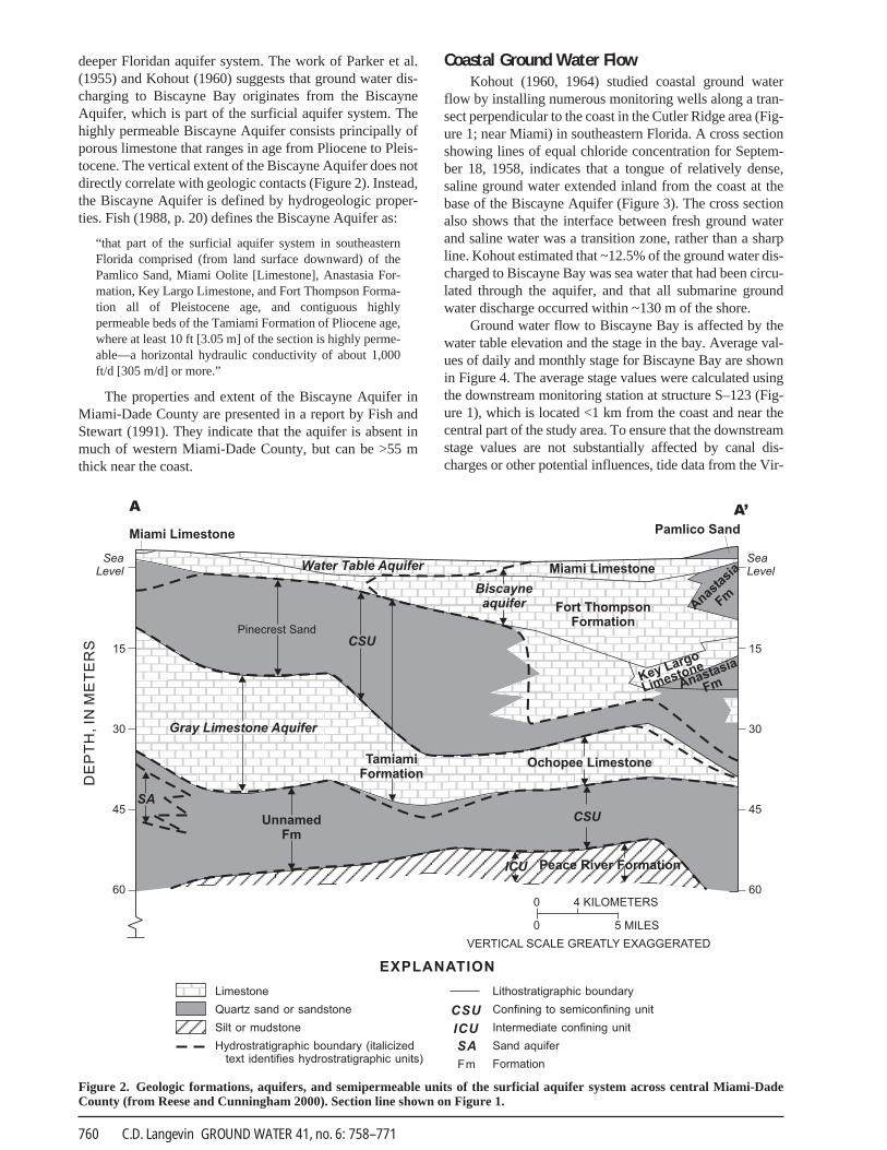
Coastal Ground Water FlowKohout (1960, 1964) studied coastal ground water

flow by installing numerous monitoring wells along a tran-sect perpendicular to the coast in the Cutler Ridge area (Fig-ure 1; near Miami) in southeastern Florida. A cross sectionshowing lines of equal chloride concentration for Septem-ber 18, 1958, indicates that a tongue of relatively dense,saline ground water extended inland from the coast at thebase of the Biscayne Aquifer (Figure 3). The cross sectionalso shows that the interface between fresh ground waterand saline water was a transition zone, rather than a sharpline. Kohout estimated that ~12.5% of the ground water dis-charged to Biscayne Bay was sea water that had been circu-lated through the aquifer, and that all submarine groundwater discharge occurred within ~130 m of the shore.

Ground water flow to Biscayne Bay is affected by thewater table elevation and the stage in the bay. Average val-ues of daily and monthly stage for Biscayne Bay are shownin Figure 4. The average stage values were calculated usingthe downstream monitoring station at structure S–123 (Fig-ure 1), which is located <1 km from the coast and near thecentral part of the study area. To ensure that the downstreamstage values are not substantially affected by canal dis-charges or other potential influences, tide data from the Vir-

C.D. Langevin GROUND WATER 41, no. 6: 758–771760

EXPLANATION

A A’

VERTICAL SCALE GREATLY EXAGGERATED

5 MILES

4 KILOMETERS0

0

CSU

ICU

SA

Fm

Pamlico Sand

Ochopee Limestone

Pinecrest Sand

UnnamedFm

Key Largo

Limestone

Fort ThompsonFormation

SA

Anas

tasi

a

Fm

Anastasia

Fm

Miami Limestone

Biscayneaquifer

Miami Limestone

TamiamiFormation

CSU

CSU

Peace River Formation

SeaLevel

DE

PT

H,IN

ME

TE

RS 15

30

45

60

SeaLevel

15

30

45

60

Water Table Aquifer

Gray Limestone Aquifer

Limestone

Quartz sand or sandstone

Silt or mudstone

Hydrostratigraphic boundary (italicizedtext identifies hydrostratigraphic units)

Lithostratigraphic boundary

Confining to semiconfining unit

Intermediate confining unit

Sand aquifer

Formation

ICU

Figure 2. Geologic formations, aquifers, and semipermeable units of the surficial aquifer system across central Miami-DadeCounty (from Reese and Cunningham 2000). Section line shown on Figure 1.

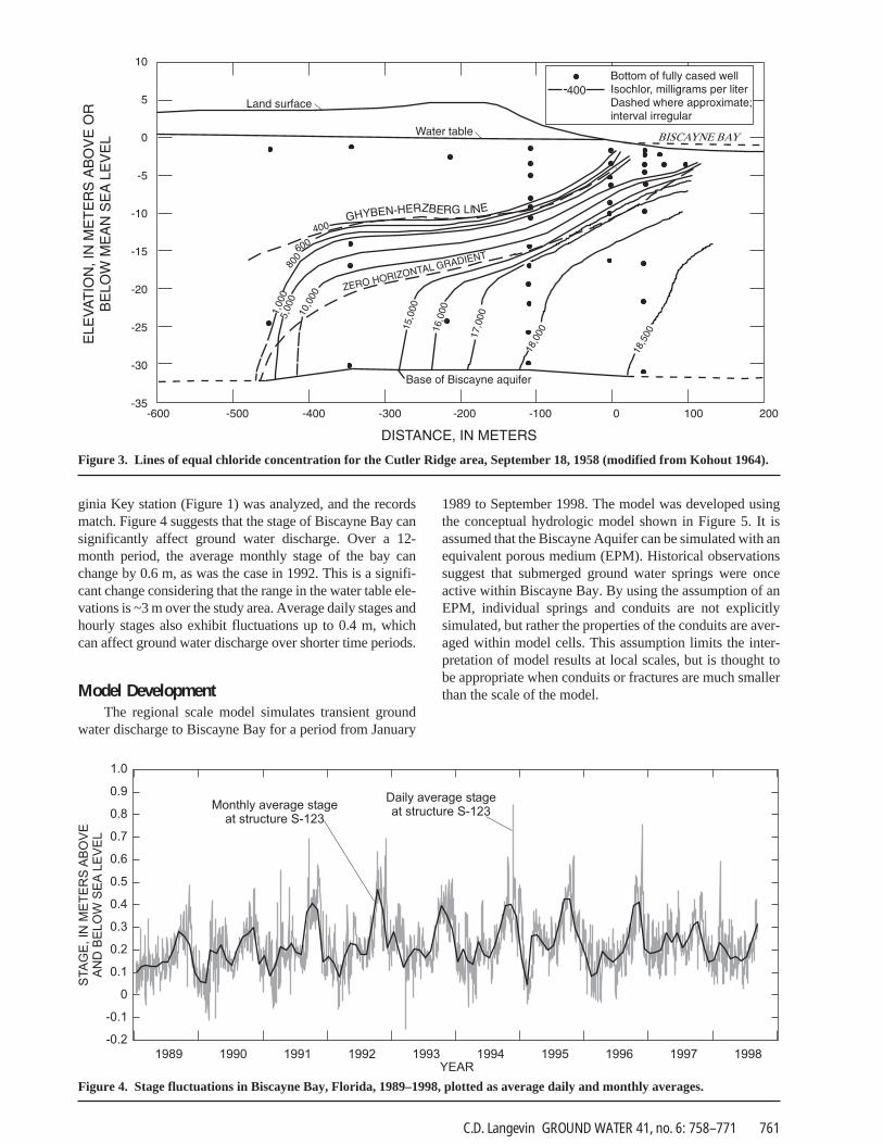
ginia Key station (Figure 1) was analyzed, and the recordsmatch. Figure 4 suggests that the stage of Biscayne Bay cansignificantly affect ground water discharge. Over a 12-month period, the average monthly stage of the bay canchange by 0.6 m, as was the case in 1992. This is a signifi-cant change considering that the range in the water table ele-vations is ~3 m over the study area. Average daily stages andhourly stages also exhibit fluctuations up to 0.4 m, whichcan affect ground water discharge over shorter time periods.

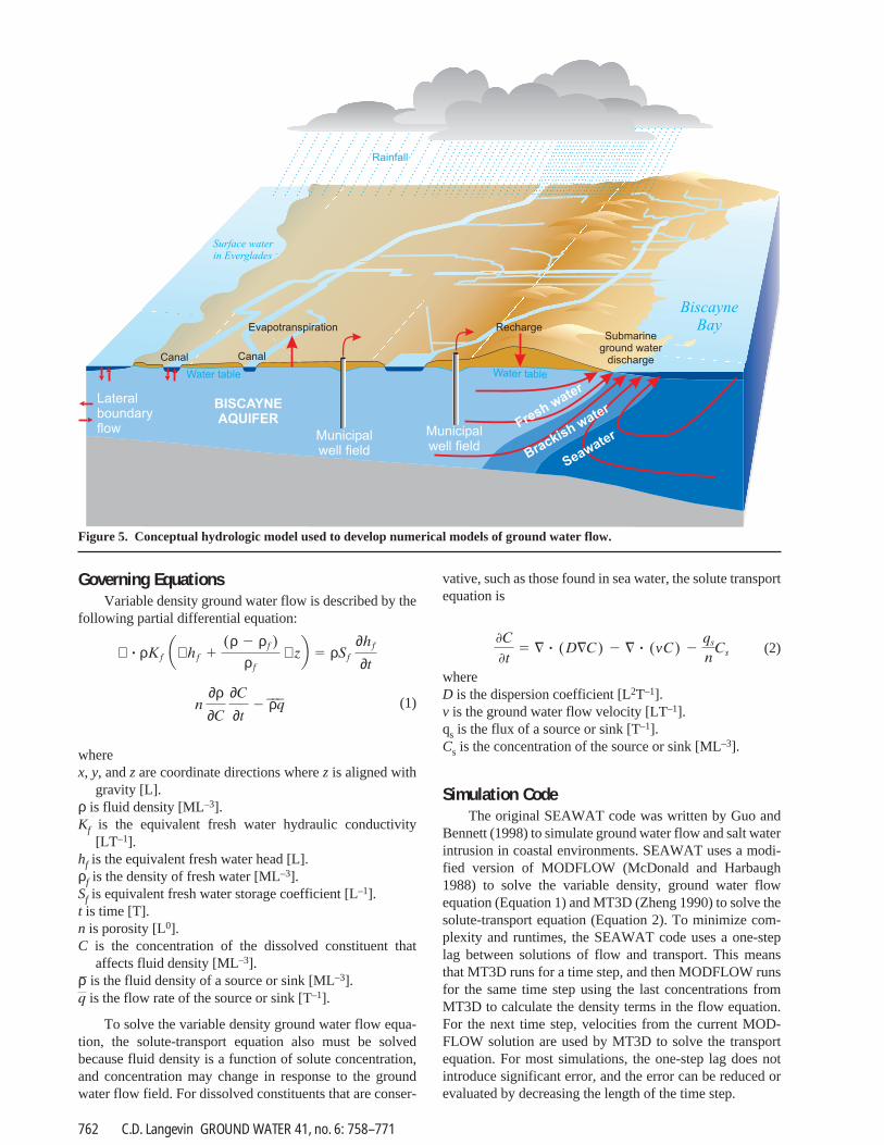
Model DevelopmentThe regional scale model simulates transient ground

water discharge to Biscayne Bay for a period from January

1989 to September 1998. The model was developed usingthe conceptual hydrologic model shown in Figure 5. It isassumed that the Biscayne Aquifer can be simulated with anequivalent porous medium (EPM). Historical observationssuggest that submerged ground water springs were onceactive within Biscayne Bay. By using the assumption of anEPM, individual springs and conduits are not explicitlysimulated, but rather the properties of the conduits are aver-aged within model cells. This assumption limits the inter-pretation of model results at local scales, but is thought tobe appropriate when conduits or fractures are much smallerthan the scale of the model.

761C.D. Langevin GROUND WATER 41, no. 6: 758–771

18,5

00

18,0

0017,0

00

16,0

00

15,0

00

10,0

00

5,0

00

1,0

00

800

600

400GHYBEN-HERZBERG LINE

Water table

ZERO HORIZONTAL GRADIENT

Base of Biscayne aquifer

BISCAYNE BAY

DISTANCE, IN METERS

EL

EV

AT

ION

,IN

ME

TE

RS

AB

OV

EO

RB

EL

OW

ME

AN

SE

AL

EV

EL

Land surface

-600 -500 -400 -300 -200 -100 0 100 200

10

5

0

-5

-10

-15

-20

-25

-30

-35

Bottom of fully cased wellIsochlor, milligrams per literDashed where approximate;interval irregular

400

Figure 3. Lines of equal chloride concentration for the Cutler Ridge area, September 18, 1958 (modified from Kohout 1964).

1989 1990 1991 1992 1993 1994 1995 1996 1997 1998YEAR

1.0

0.9

0.8

0.7

0.6

0.5

0.4

0.3

0.2

0.1

0

-0.1

-0.2

STA

GE

,IN

ME

TE

RS

AB

OV

EA

ND

BE

LO

WS

EA

LE

VE

L

Daily average stageat structure S-123

Monthly average stageat structure S-123

Figure 4. Stage fluctuations in Biscayne Bay, Florida, 1989–1998, plotted as average daily and monthly averages.

Governing EquationsVariable density ground water flow is described by the

following partial differential equation:

(1)

wherex, y, and z are coordinate directions where z is aligned with

gravity [L].ρ is fluid density [ML–3].Kf is the equivalent fresh water hydraulic conductivity

[LT–1].hf is the equivalent fresh water head [L].ρf is the density of fresh water [ML–3].Sf is equivalent fresh water storage coefficient [L–1].t is time [T].n is porosity [L0].C is the concentration of the dissolved constituent that

affects fluid density [ML–3].ρ_

is the fluid density of a source or sink [ML–3].is the flow rate of the source or sink [T–1].

To solve the variable density ground water flow equa-tion, the solute-transport equation also must be solvedbecause fluid density is a function of solute concentration,and concentration may change in response to the groundwater flow field. For dissolved constituents that are conser-

q

n ∂ρ∂C

∂C

∂t2 ρq

___

∇ � ρKf a∇ hf 1(ρ 2 ρf)

ρf ∇ zb 5 ρSf

∂hf

∂t

vative, such as those found in sea water, the solute transportequation is

(2)

whereD is the dispersion coefficient [L2T–1].v is the ground water flow velocity [LT–1].qs is the flux of a source or sink [T–1].Cs is the concentration of the source or sink [ML–3].

Simulation CodeThe original SEAWAT code was written by Guo and

Bennett (1998) to simulate ground water flow and salt waterintrusion in coastal environments. SEAWAT uses a modi-fied version of MODFLOW (McDonald and Harbaugh1988) to solve the variable density, ground water flowequation (Equation 1) and MT3D (Zheng 1990) to solve thesolute-transport equation (Equation 2). To minimize com-plexity and runtimes, the SEAWAT code uses a one-steplag between solutions of flow and transport. This meansthat MT3D runs for a time step, and then MODFLOW runsfor the same time step using the last concentrations fromMT3D to calculate the density terms in the flow equation.For the next time step, velocities from the current MOD-FLOW solution are used by MT3D to solve the transportequation. For most simulations, the one-step lag does notintroduce significant error, and the error can be reduced orevaluated by decreasing the length of the time step.

'C't

5 = ? (D=C) 2 = ? (vC) 2qs

nCs

C.D. Langevin GROUND WATER 41, no. 6: 758–771762

BiscayneBay

Municipalwell field

Evapotranspiration

Surface waterin Everglades

Recharge

Lateralboundaryflow

Brackish water

Fresh water

Seawater

Submarineground water

discharge

BISCAYNEAQUIFER

Canal Canal

Water table Water table

Rainfall

Municipalwell field

Figure 5. Conceptual hydrologic model used to develop numerical models of ground water flow.

One major reason the SEAWAT code was selected forthis study is that it uses MT3D to solve the transport equa-tion. MT3D contains a variety of methods for solving thetransport equation including the method of characteristics(MOC). During the simulation of solute transport, numeri-cal dispersion and other problems (long computer runtimes,temporal and spatial resolution requirements, etc.) often areencountered. With SEAWAT, an acceptable solution canusually be obtained because MT3D has a variety of solutiontechniques, including MOC, which is ideal for reducingnumerical dispersion. For the simulations presented in thispaper, MOC was used with 16 to 256 particles per cell.

Another advantage of using SEAWAT is that it uses twowidely accepted modeling codes: MODFLOW and MT3D,which means that SEAWAT is modular and contains the“package” approach for including various boundary condi-tions and transport options. As a result, SEAWAT containspackages, such as the drain and river, which are conceptuallysimilar to the equivalent packages in MODFLOW. In addi-tion, SEAWAT reads and writes standard MODFLOW andMT3D data files, which are easily manipulated with com-mercially available pre- and post-processors.

The original SEAWAT code (Guo and Bennett 1998),referred to as version 1, was modified for this study of Bis-cayne Bay. Langevin and Guo (1999) and Langevin (2001)present a description of those modifications. Guo andLangevin (2002) present the formal documentation for ver-sion 2 of the SEAWAT code, which was released by theU.S. Geological Survey after the completion of the Bis-cayne Bay study. Version 2 contains a newer version ofMT3D (Zheng and Wang 1998) and is distributed withinthe public domain.

Spatial and Temporal DiscretizationTo simulate ground water flow to Biscayne Bay, a reg-

ularly spaced, finite-difference model grid was constructedand rotated so that the y-axis would roughly parallel thecoast (Figure 6). Each cell is 1000 m × 1000 m in the hori-zontal plane. The grid consists of 89 rows and 71 columns,and the rotation angle from true north is clockwise 14degrees. The purpose for rotating the grid is to align modelrows with the principal direction of ground water flow,which is primarily toward Biscayne Bay. When groundwater flow is not parallel to one of the primary model axes,some numerical schemes can experience accuracy prob-lems in the solution to the transport equation. Another rea-son for rotating the model grid is that future modificationsto the model may require a higher level of discretization atthe coast. A rotated model grid allows the resolution alonga flow line to be increased by dividing columns near thecoast. To maintain reasonable computer runtimes, thedomain of the regional model was not extended south toFlorida Bay. Future versions of the model, however, mayextend into Florida Bay as a method for eliminating poten-tial boundary effects.

Accurate simulation of variable density flow systemsrequires a finer vertical resolution compared to that requiredfor simulating constant density flow systems. Thisincreased resolution is necessary because of transport con-siderations and because vertical density gradients must be

resolved in order to calculate accurate flow velocities.Accordingly, the model grid, which represents the BiscayneAquifer, consists of 10 layers—more layers than would berequired for a typical ground water flow model that does notrepresent density variations. The top elevation of layer 1 isspatially variable and corresponds with land surface eleva-tion, based on a compiled topographic contour map pro-vided by Everglades National Park. For model cells withinBiscayne Bay, the top of layer 1 has a value of 0.0 m. Thebottom of layer 1 is set at an elevation of 5.0 m below sealevel. To minimize the effects of numerical problems thatcan occur in solute-transport models, the grid was designedso that layers would be flat and cells would have a uniformvolume (1000 m × 1000 m × 5 m). Although the volume foreach model cell in layer 1 may be slightly variable becauseof the variation in land surface elevation, model cells in lay-ers 2 through 10 have a uniform thickness of 5 m, and thusa uniform cell volume. The bottom elevation for layer 10 is50 m below sea level. The base of the Biscayne Aquifer, asdefined by Fish and Stewart (1991), generally slopes fromwest to east. This variability in aquifer thickness wasincluded in the model by inactivating model cells with cellcenters below the base of the Biscayne Aquifer.

The nearly 10-year simulation period is divided into116 monthly stress periods. For each stress period, the aver-age hydrologic conditions for that month are assumed toremain constant. This means that the model does not simu-late hourly or daily hydrologic variations, but rather sea-sonal and yearly variations. Further temporal discretizationis introduced in the form of time steps within each stress

763C.D. Langevin GROUND WATER 41, no. 6: 758–771

AT

LA

NT

ICO

CE

AN

������

������

������

�����

����� ����� �����

Florida Bay

EVERGLADESNATIONAL

PARK

CO

LLIE

RC

OU

NT

Y

MIA

MI-

DA

DE

CO

UN

TY

BROWARD COUNTY

MIAMI-DADE COUNTY

MO

NR

OE

CO

UN

TY

MIA

MI-

DA

DE

CO

UN

TY

BarnesSound

Car

dSo

und

EXPLANATION

Lake

Canal

Bis

cayn

eB

ay

MODELGRID

General-head boundary

River boundary

Figure 6. Finite-difference grid and boundary conditions inthe upper layer for the regional scale ground water flowmodel in southern Florida.

period. Each stress period is divided into one or more timesteps, the lengths of which are determined by SEAWAT tomeet specified criteria associated with solving the solute-transport equation. For the regional scale model, about 20time steps were required for each stress period.

Assignment of Aquifer ParametersThe approach for assigning aquifer parameters that

pertain to ground water flow-and-solute transport was touse the simplest distribution that would result in adequaterepresentation of the flow system. Parameter values used inthe model are listed in Table 1. Langevin (2001) provides adetailed description of how aquifer parameters were deter-mined.

Boundary ConditionsThe boundary conditions available in SEAWAT con-

sist of those packages released with the 1988 version ofMODFLOW and the time variant constant-head package.Methods for generating boundary conditions for theregional model follow the standard approaches outlined byAnderson and Woessner (1992) and Zheng and Bennett(2002). Table 2 provides a summary of the boundary condi-

tions, which are discussed in detail by Langevin (2001). Adescription of the Biscayne Bay boundary condition is pro-vided as follows.

The model cells in layer 1 representing Biscayne Baywere simulated with the time varying constant head (CHD)package in SEAWAT. By specifying a constant fresh waterhead boundary in layer 1, the elevation for the bottom ofBiscayne Bay corresponds to the center elevation of layer 1;thus, the simulated bay bottom is flat with an elevation of2.5 m. Average monthly values (Figure 4) for downstreamstage at structure S–123 were used to set the water level inthe constant-head cells. The downstream stage measure-ment at structure S–123 was used because this structure islocated at the coast and lies near the center of the BiscayneBay shoreline. Results from a calibrated hydrodynamic cir-culation model, which covers all but the northernmost partof Biscayne Bay, suggest that the salinity in the bay is tem-porally and spatially variable because of surface water dis-charge (Wang 2001). Results from the circulation modelwere used to set spatially varying and temporally varyingconcentration values for the constant concentration andconstant-head cells representing Biscayne Bay. The fewdata that exist for the northern part of Biscayne Bay suggestthat salinity for the northern area may be lower than that ofsea water; however, a constant value of 35 kg/m3 was spec-

C.D. Langevin GROUND WATER 41, no. 6: 758–771764

Table 1Aquifer Parameters Used in the Regional Scale Ground Water Flow and Transport Model

Parameter Description Comment

Hydraulic conductivity (m/d)

Zone 11: Kh = 9000Kv = 90

Zone 21: Kh = 3Kv = 0.3

Zone 31: Kh = 1500Kv = 15

Primary and secondary storage coefficient2

(unitless)

Layer 1: SF1 = 1.0SF2 = 0.2

Layers 2–10: SF1 = 5.9 � 10–5

SF2 = 0.2

Porosity (unitless)

Uniform value: n = 0.2

Dispersivity (m)Uniform values: �L = 5.0

�T = 0.5

Value used in calibrated flow model by Merritt (1996) to representMiami Limestone, Fort Thompson, and permeable zones of theTamiami Formation

Value assigned to represent peat and marl units in the upper part of theBiscayne Aquifer

Value assigned by Merritt (1996) to match flow and head patterns nearcentral Biscayne Bay

Primary coefficient used for infrequent case when water table risesabove land surface; secondary value equal to specific yield estimated byMerritt (1996)

Primary coefficient estimated using compressibility for fractured rock(2 � 10–10 m2/N; Domenico and Schwartz 1990, p. 111); secondaryvalue equal to specific yield estimated by Merritt (1996)

Assumed porosity of porous limestone similar to specific yield estimatedby Merritt (1996)

Dispersivity values determined through calibration of two cross-sectionmodels with fine horizontal and vertical resolution (Langevin 2001)

1Zone boundaries shown in Langevin (2001; Plate 3)2Primary storage coefficient used by the model when head is above top elevation of cell; secondary storage coefficient used when water table located within cell(McDonald and Harbaugh 1988)

Note: Kh, horizontal hydraulic conductivity; Kv, vertical hydraulic conductivity; SF1, primary storage coefficient; SF2, secondary storage coefficient; n, porosity;αL, longitudinal dispersivity; αT, transverse dispersivity

ified for the part of Biscayne Bay not covered by the circu-lation model. The model results from Wang (2001) suggestthat the salinity of central Biscayne Bay ranges from ~15 to35 kg/m3 at the shoreline, 20 to 35 kg/m3 at a distance of5500 m from the shoreline, and 25 to 35 kg/m3 at a distanceof 13,500 m from the shoreline. In the circulation model,the larger fluctuation in salinity near the coast is primarilydue to significant fresh water discharges at canal mouths.

Initial ConditionsInitial water levels were specified for the model by

interpolating values from a two-dimensional representationof the water table surface for January 1989. For most mod-eling applications, the use of field data to specify initialwater levels can introduce model error at the beginning ofthe simulation; however, for the highly permeable BiscayneAquifer, numerical experiments have shown that errorsintroduced by specifying initial water levels with field dataare eliminated several weeks into the simulation. Earlyattempts to specify initial concentrations consisted of run-

ning the model over and over until the position of the inter-face reached dynamic equilibrium. The position of theinterface at dynamic equilibrium, however, was too farinland for the northern part of the model. Due to the lower-ing of the water table beginning in the early 1900s, theinterface position may not be at equilibrium. Thus, thedynamic equilibrium approach for setting initial concentra-tions was replaced with a hybrid method developed by trialand error. Later attempts to set initial concentrations usedthe 1995 salt water intrusion line by Sonenshein (1997),who delineated the position of the interface at the base ofthe Biscayne Aquifer using chloride concentrations frommonitoring wells and time-domain electromagnetic sound-ings. The first attempt with the 1995 salt water intrusionline, which is nearly identical to the 1984 salt water intru-sion line mapped by Klein and Waller (1985), consisted ofspecifying sea water concentrations (35 kg/m3) east of theline and fresh water concentrations west of the salt waterintrusion line. This procedure for specifying initial concen-trations was used for each layer and resulted in a verticalwall of sea water at the 1995 salt water intrusion line.

765C.D. Langevin GROUND WATER 41, no. 6: 758–771

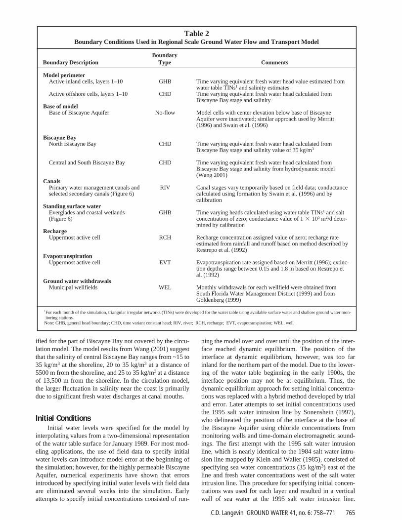
Table 2Boundary Conditions Used in Regional Scale Ground Water Flow and Transport Model

BoundaryBoundary Description Type Comments

Model perimeterActive inland cells, layers 1–10 GHB

Active offshore cells, layers 1–10 CHD

Base of modelBase of Biscayne Aquifer No-flow

Biscayne BayNorth Biscayne Bay CHD

Central and South Biscayne Bay CHD

CanalsPrimary water management canals and RIVselected secondary canals (Figure 6)

Standing surface waterEverglades and coastal wetlands GHB(Figure 6)

RechargeUppermost active cell RCH

EvapotranspirationUppermost active cell EVT

Ground water withdrawalsMunicipal wellfields WEL

Time varying equivalent fresh water head value estimated fromwater table TINs1 and salinity estimatesTime varying equivalent fresh water head calculated from Biscayne Bay stage and salinity

Model cells with center elevation below base of BiscayneAquifer were inactivated; similar approach used by Merritt(1996) and Swain et al. (1996)

Time varying equivalent fresh water head calculated fromBiscayne Bay stage and salinity value of 35 kg/m3

Time varying equivalent fresh water head calculated fromBiscayne Bay stage and salinity from hydrodynamic model(Wang 2001)

Canal stages vary temporarily based on field data; conductancecalculated using formation by Swain et al. (1996) and bycalibration

Time varying heads calculated using water table TINs1 and saltconcentration of zero; conductance value of 1 � 105 m2/d deter-mined by calibration

Recharge concentration assigned value of zero; recharge rateestimated from rainfall and runoff based on method described byRestrepo et al. (1992)

Evapotranspiration rate assigned based on Merritt (1996); extinc-tion depths range between 0.15 and 1.8 m based on Restrepo etal. (1992)

Monthly withdrawals for each wellfield were obtained fromSouth Florida Water Management District (1999) and fromGoldenberg (1999)

1For each month of the simulation, triangular irregular networks (TINs) were developed for the water table using available surface water and shallow ground water mon-itoring stations.

Note: GHB, general head boundary; CHD, time variant constant head; RIV, river; RCH, recharge; EVT, evapotranspiration; WEL, well

Results from early simulations suggested that a better esti-mate for initial salinity concentrations would reduce thelength of simulation time required to achieve a stable posi-tion for the salt water interface, thus increasing the length oftime model results would be unaffected by the initial salin-ity distribution. The initial salinity distribution wasimproved by linearly interpolating concentrations betweenthe 1995 salt water intrusion line and Biscayne Bay. Theinitial salinity distribution was further improved by incor-porating the results from an airborne geophysical survey(Fitterman and Deszcz-Pan 1998) of the southern part of themodel area.

Model CalibrationThe regional scale model was calibrated using trial and

error by matching heads, ground water exchange rates withcanals, and position of the salt water interface. The meanerror (ME) in head for all stress periods and wells (6525values in total) is 0.08 m. The positive value for ME indi-cates that simulated values of head generally are higher thanobserved values of head. The mean absolute error (MAE) is0.15 m, which is an acceptable value considering thatobserved heads range from �2.23 to 2.51 m. This meansthat the MAE relative to the range in observed heads is~3%. The root mean square error (RMSE) is 0.27 m, indi-cating that ~68% of the head differences are within ±0.27 mof the ME. A histogram constructed from the differencesbetween observed and simulated heads suggests that thedifferences are normally distributed with a mode of ~0.05m. Langevin (2001) presents a more thorough comparisonof observed versus simulated water levels.

Calibration of the regional scale model to canal base-flow was performed for surface water basins (Cooper andLane 1987) with measured surface water inflows and out-flows. For each of these basins, simulated baseflow wascombined with the total runoff value estimated from theland-use method described earlier. This combined valuewas then compared with the net canal loss or gain measuredfor the basin. Net losses and gains were calculated for theselected surface water basins by subtracting canal inflowsfrom canal outflows. It is assumed that the differencebetween inflow and outflow is equal to baseflow andrunoff. The mathematical equation is:

baseflow + runoff = canal outflow – canal inflow

where the left side of the equation is based on the simulationand the right side is based on measured quantities. The flowterms on the right side of the equation, originally calculatedfrom rating curves at structures, were obtained from thedatabase of the SFWMD. Canal outflow is the sum of allsurface water discharge that flows out of the surface waterbasin. Canal inflow is the sum of all surface water dischargethat flows into the surface water basin. This approachassumes that direct rainfall to a canal, direct evaporationfrom a canal, and storage within a canal are negligible. Forthe 12 surface water basins used in the calibration, the meanabsolute error between observed and simulated baseflowand runoff ranges between 1.9 × 105 and 5.5 × 105 m3/day.The mean difference between measured canal outflow and

canal inflow, combined for the 12 surface water basins, is3.1 � 106 m3/day.

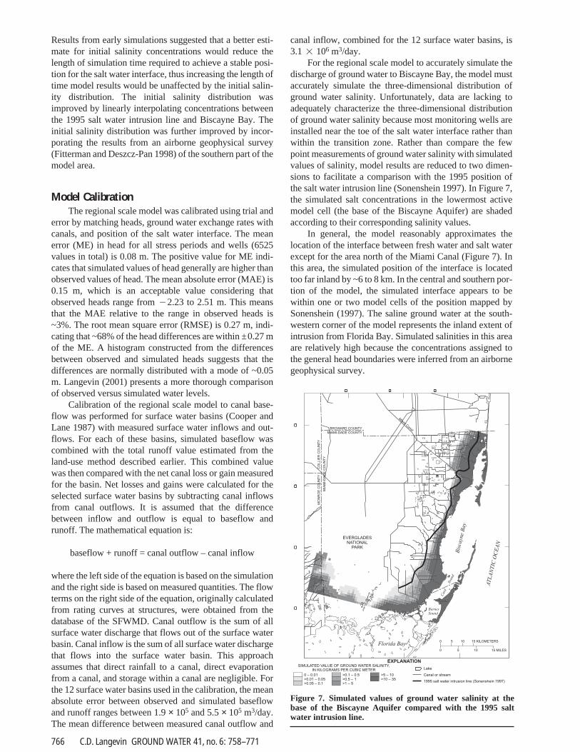
For the regional scale model to accurately simulate thedischarge of ground water to Biscayne Bay, the model mustaccurately simulate the three-dimensional distribution ofground water salinity. Unfortunately, data are lacking toadequately characterize the three-dimensional distributionof ground water salinity because most monitoring wells areinstalled near the toe of the salt water interface rather thanwithin the transition zone. Rather than compare the fewpoint measurements of ground water salinity with simulatedvalues of salinity, model results are reduced to two dimen-sions to facilitate a comparison with the 1995 position ofthe salt water intrusion line (Sonenshein 1997). In Figure 7,the simulated salt concentrations in the lowermost activemodel cell (the base of the Biscayne Aquifer) are shadedaccording to their corresponding salinity values.

In general, the model reasonably approximates thelocation of the interface between fresh water and salt waterexcept for the area north of the Miami Canal (Figure 7). Inthis area, the simulated position of the interface is locatedtoo far inland by ~6 to 8 km. In the central and southern por-tion of the model, the simulated interface appears to bewithin one or two model cells of the position mapped bySonenshein (1997). The saline ground water at the south-western corner of the model represents the inland extent ofintrusion from Florida Bay. Simulated salinities in this areaare relatively high because the concentrations assigned tothe general head boundaries were inferred from an airbornegeophysical survey.

C.D. Langevin GROUND WATER 41, no. 6: 758–771766

SIMULATED VALUE OF GROUND WATER SALINITY,IN KILOGRAMS PER CUBIC METER

AT

LA

NT

ICO

CE

AN

Bis

cayn

eB

ay

������

������

������

�����

����� ����� �����

Florida Bay

EVERGLADESNATIONAL

PARK

CO

LLIE

RC

OU

NT

Y

MIA

MI-

DA

DE

CO

UN

TY

EXPLANATION

BROWARD COUNTY

MIAMI-DADE COUNTY

MO

NR

OE

CO

UN

TY

BarnesSound

Car

dSo

und

0 15 KILOMETERS5 10

0 15 MILES5 10

0 – 0.01>0.01 – 0.05>0.05 – 0.1

>0.1 – 0.5>0.5 – 1>1 – 5

>5 – 10>10 – 35

Lake

Canal or stream

1995 salt water intrusion line (Sonenshein 1997)

Miam

i Canal

Figure 7. Simulated values of ground water salinity at thebase of the Biscayne Aquifer compared with the 1995 saltwater intrusion line.

There are several possible explanations for the discrep-ancy in the northern part of the model. First, the simulatedground water heads in this area may be too low, which is thecase for one of the coastal monitoring wells in this area.Simulated heads that are too low may have been caused bya lack of sufficient head data that resulted in assignment ofinappropriate aquifer parameters or hydrologic stresses,such as recharge or evapotranspiration. Another possibleexplanation for the poor match north of Miami Canal is thatthe model may not accurately represent the process of dis-persion in this area. Konikow and Reilly (1999) discuss therationale behind the concept that dispersion prevents theinterface from moving inland in north Miami-Dade Countyto a position predicted by the Ghyben-Herzberg principle.Thus, if the model does not simulate enough dispersion, thesimulated interface will be located too far inland. A thirdpossible explanation for the poor match is that the boundarycondition used to represent Biscayne Bay may not be setappropriately. In the model, an equivalent fresh water headvalue was calculated for the constant-head cells represent-ing Biscayne Bay using the density of sea water (1025kg/m3). Thus, if the actual density of north Biscayne Baywas less than sea water, the equivalent fresh water headwould be lower, and the interface would not move as farinland. Additional research is necessary to determine whichof these explanations, or combination of explanations, ismost likely.

Simulated Estimates of Submarine GroundWater Discharge to Biscayne Bay

The simulated ground water flow from the activemodel cells into the coastal constant-head cells is assumedto represent the discharge of ground water to Biscayne Bay.In addition to simulating the volumetric flow rate, themodel also simulates the salt concentration of the groundwater flow into the constant-head cells. This salt concentra-tion is assumed to represent the salinity of the ground waterthat discharges to Biscayne Bay. The simulated salinity ofground water discharge to Biscayne Bay ranges from nearlyfresh at the shoreline to nearly sea water some distance off-shore. To simplify the results, simulated discharge esti-mates are presented as the fresh water portion of the totaldischarge. The fresh water portion of the ground water dis-charge is calculated from the total discharge using the fol-lowing equation:

(3)

where:Qf is simulated fresh ground water discharge, in m3/day.QT is simulated total ground water discharge, in m3/day.ρs is fluid density of sea water, in kg/m3.ρ is simulated fluid density of ground water discharging to

Biscayne Bay, in kg/m3.

When the fluid density of the ground water discharge isequal to 1000 kg/m3, the fresh ground water discharge isequal to the total ground water discharge. When the fluiddensity of the ground water discharge is equal to the fluid

Qf 5 QT(�s 2 �)(�s 2 �f)

density of sea water (1025 kg/m3), the fresh ground waterdischarge is equal to zero. During certain times, simulatedflow is from the bay into the aquifer. When this conditionoccurs, QT is negative, but Qf is zero. A subroutine wasadded to SEAWAT to calculate and sum the QT and Qfterms between each constant-head cell and the adjacentactive cells. These flow terms are written to a file followingeach time step. At the end of a model run, a post-processingroutine calculates the average flows for each constant-headcell by stress period.

One potential problem with calculating fresh groundwater discharge estimates from simulated density is that theresulting fresh water discharge quantities are directlydependent on salt concentrations. (Density is a linear func-tion of salt concentration.) As previously mentioned,ground water salinities are considered calibrated when thesimulated position of the salt water toe matches with theobserved position. This does not ensure that the simulatedsalt concentrations are calibrated. The average salt concen-tration of simulated discharge to Biscayne Bay is about halfthat of sea water, and thus half of the total discharge is freshwater. This suggests that if salt concentrations were in errorby 100% (17.5 kg/m3), estimates of fresh ground water dis-charge might be in error by about a factor of two.

Results from the regional scale model indicate thatfresh and brackish ground water discharges to BiscayneBay along the coastline and into the tidal portions of theMiami, Coral Gables, and Snapper Creek Canals (locationsshown in Figure 1). The model suggests that fresh groundwater discharge at the coastline of Biscayne Bay is similarin magnitude to the fresh ground water discharge to tidalcanals. The average rate of fresh ground water discharge is~3.7 � 105 m3/day for the coastline of Biscayne Bay, about1.8 � 105 m3/day for the tidal portion of the Miami Canal,~1.4 � 105 m3/day for the tidal portion of the Coral GablesCanal, and ~3.4 � 104 m3/day for the tidal portion of theSnapper Creek Canal. The annual fluctuation in freshground water discharge is ~1 � 105 m3/day for the coast-line of Biscayne Bay and the tidal portions of the Miami andCoral Gables Canals, and ~3 � 104 m3/day for the tidal por-tion of the Snapper Creek Canal. Fluctuations in groundwater discharge appear to be dampened because sea levelwas highest during the wet season when the water table wasrelatively high and lowest during the dry season when thewater table was relatively low.

A comparison was made between simulated freshground water discharge and measured surface water dis-charge from the coastal control structures. Based on theresults for the simulation period (1989–1998), fresh groundwater discharge seems to be an important mechanism offresh water delivery to Biscayne Bay during some dry sea-sons (Figure 8). For the dry seasons of 1989, 1990, and1991, model results suggest that fresh ground water dis-charge exceeded the surface water discharge to BiscayneBay. During the wet season, however, fresh ground waterdischarge is about an order of magnitude less than the sur-face water discharge. For the total simulation period,ground water discharge directly to Biscayne Bay is ~10% ofsurface water discharge, or 2% of annual rainfall over theactive model domain.

767C.D. Langevin GROUND WATER 41, no. 6: 758–771

Nearly 100% of the fresh ground water discharge toBiscayne Bay is to the northern half of the bay, north ofstructure S–123 (Figure 1). South of structure S–123 (Fig-ure 1), where land surface elevations are <1 m above sealevel, the water table was unable to develop enough head todrive ground water discharge into the bay. In this area,evapotranspiration from coastal wetlands is the dominanthydrologic process. If simulated salinities for the northernpart of the model were improved, there may be even higherrates of fresh submarine ground water discharge to thenorthern half of Biscayne Bay.

Sensitivity to Biscayne Bay Boundary ConditionBy using the specified concentration boundary condi-

tion (also referred to as Type I or Dirichlet boundary) forBiscayne Bay, solute enters the active aquifer domainthrough advection and dispersion. This type of boundarycondition was selected to represent Biscayne Bay becausethe model uses monthly stress periods; therefore, dispersionbeneath Biscayne Bay as a result of tidal and daily fluctua-tions in stage was not directly included in the model. It wasassumed that the dispersion caused by these relatively highfrequency variations in stage could be represented with thedispersive salt flux that results from using the constant con-centration boundary condition. There was, however, nodirect evidence to support the selection of this type ofboundary condition for solute transport, nor was there anadequate method for assigning an appropriate dispersioncoefficient or dispersivity value. A mixed condition (TypeIII or Cauchy boundary) is another boundary type availablein SEAWAT and can be used with a constant-head boundary(Zheng and Bennett 2002). With the mixed-boundary condi-tion in SEAWAT, inflow from the boundary is assigned auser-specified concentration, whereas outflow to the bound-ary carries the concentration calculated at the active celladjacent to the boundary. Regardless of the flow direction,the concentration gradient is held at zero, which eliminatesthe dispersive flux across the boundary. The following sen-

sitivity analysis was performed to evaluate the effects ofboundary type on discharge rates to Biscayne Bay.

To evaluate the effects of solute-transport boundarytype on simulated rates of fresh ground water discharge,another simulation was run in which a mixed boundary wasspecified with concentration values from the circulationmodel. By using a mixed boundary rather than holding theconcentration constant, salt mass enters the active aquiferdomain only through advection. For this simulation, theaverage rate of fresh ground water discharge directly to Bis-cayne Bay is 5.8 � 105 m3/day, or 55% more than for thesimulation with a constant concentration boundary (referredto as the base case). The reason that the rate of fresh groundwater discharge is 55% more for this simulation is becausethe simulated salt concentrations beneath the bay are lessthan the simulated concentrations in the base case. With theconstant concentration boundary, salt mass enters throughadvection and dispersion, causing simulated concentrationsto be relatively high beneath the bay (as in the base case).Therefore, the fresh ground water discharge, which is cal-culated from the actual discharge and the discharge concen-tration, tends to be larger with a mixed boundary. Onepossible method for reducing the quantity of salt mass thatenters the aquifer from a constant concentration boundaryby dispersion is to lower the dispersivity values near theboundary.

The effects of bay salinity on ground water dischargewere evaluated by running a simulation in which a salinityvalue of 35 kg/m3 was specified for the entire bay, a simpli-fied assumption that was originally used in the model devel-opment. For this case, the average rate of simulated freshground water discharge directly to Biscayne Bay is 2.2 �105 m3/day, ~40% less than for the base case. This rate isless than the base case for two reasons: First, the equivalentfresh water head value assigned to the constant-head cells ishigher because the density of the bay water is higher. Sec-ond, in the base case, a portion of the “fresh” discharge mayactually be brackish water that entered the aquifer from Bis-cayne Bay rather than from inland recharge. When the con-centration is fixed at 35 kg/m3, this extra source of partiallyfresh bay water is eliminated, and salt concentrationsbeneath the bay are higher. The result is a lower calculatedflux of fresh discharge to the bay.

Another simulation also was run with the salinity valueof 35 kg/m3 used with the mixed boundary type. For thiscase, the average rate of simulated fresh ground water dis-charge directly to Biscayne Bay is 4.9 � 105 m3/day, ~30%more than the rate simulated with the base case. Based onthis comparison, the boundary type seems to affect the freshdischarge rates more than the salinity values used to repre-sent the bay.

These sensitivity simulations illustrate the importanceof the boundary condition used to represent a marine estu-ary. Because the quantity of fresh ground water dischargedepends on the solute concentrations adjacent to andbeneath the estuary, slight variations in the boundary-con-dition type and the specified concentration value can have alarge effect on the simulated rate. For the Biscayne Baymodel, the use of a specified concentration boundary resultsin less fresh ground water discharge compared to a similarmodel that uses a mixed boundary. Additionally, the model

C.D. Langevin GROUND WATER 41, no. 6: 758–771768

1989 1990 1991 1992 1993 1994 1995 1996 1997 1998YEAR

0

2,000,000

4,000,000

6,000,000

8,000,000

10,000,000

12,000,000

14,000,000

16,000,000

DIS

CH

AR

GE

,IN

CU

BIC

METER

SPER

DAY

Measured surface waterdischarge to Biscayne Bay

Simulated fresh groundwater discharge directlyto Biscayne Bay

Figure 8. Simulated rates of fresh ground water dischargecompared with measured rate of surface water discharge to Bis-cayne Bay.

horizontal grid resolution. As grid spacing decreases from1000 to 31.25 m, the total flux of sea water through the sys-tem increases by a factor of five. This means that morerefined models may be required if simulated discharge ratesare compared with the total brackish water flux measuredwith seepage meters.

Discussion and ConclusionsRegional scale simulation of variable density ground

water flow is rarely performed in three dimensions becauseof limitations in computer speed, data availability, andavailability of a simulation tool that can minimize numeri-cal dispersion. The development and application of theregional scale model presented in this paper suggests thatlarge-scale simulation of variable density ground waterflow is a viable method for simulating complex groundwater flow processes in coastal environments and can beused to quantify rates of submarine ground water discharge.The modeling approach presented in this paper also couldbe used to evaluate and help manage salt water intrusion inshallow coastal aquifers.

Results from the three-dimensional, variable densityground water flow model suggest that ground water dis-charges directly to Biscayne Bay and to the tidal portions ofthe coastal canals. From January 1989 to September 1998,

results suggest that fresh ground water discharge rates aresensitive to the salinity of the estuary. Fresh discharge ratestend to increase when the salinity of the estuary decreases.

Sensitivity of Fresh Discharge to HorizontalGrid Resolution

An analysis was performed to evaluate the sensitivityof simulated submarine ground water discharge estimates tohorizontal grid resolution. Rather than perform the analysiswith the three-dimensional regional model, which wouldrequire unreasonably long simulation times, a simple crosssection model was developed using representative BiscayneAquifer parameters (Figure 9). A head-dependent boundary(GHB) was used as the inland boundary, as opposed to aspecified flux, so the net fresh water flux to the bay wouldbe calculated by the model rather than specified as input.Fresh ground water enters from the GHB cells, flowstoward the coast, and discharges into the constant headcells. A flux of sea water into the aquifer is required fromsome of the constant-head cells to provide a source of saltfor the brackish ground water that discharges into the con-stant-head cells.

Seven simulations were performed, each with differenthorizontal grid spacing within the transition zone. In thegrid design for each simulation, the horizontal node spacingbetween adjacent cells did not vary by more than a factor of1.5. Simulations were run until steady-state flow and trans-port conditions were achieved (~10,000 days). Table 3 liststhe rates of simulated fresh water inflows from the general-head boundary and sea water inflows from the constant-head boundary. Rates are expressed as m3/day per meter ofshoreline, or m2/day. The analysis suggests that, for the casetested, the rate of fresh submarine ground water dischargeto the constant-head cells does not significantly depend onthe horizontal grid spacing. Salinity contours for the sevensimulations (not shown) also were identical, except in theupper layers near the constant-head boundary. The freshdischarge estimate with 1000 m grid resolution (resolutionused in regional model) is only ~7% less than the simulatedestimate from the model with 31.25 m resolution. The rateof circulated sea water, however, is highly dependent on

EXPLANATION

General head boundaryhead = 0.79 m, inflow concentration = 0

Constant head, constant concentration boundaryhead = 0.22 m, concentration = 35 kg/m

3

vertical exaggeration = 60X

9 km 5 km

35

m

K = 9000 m/d

K = 90 m/d

n = 0.2

= 5 m

= 0.5 m

h

v

L

T

��

1000 m horizontal cell

250 m horizontal cell

769C.D. Langevin GROUND WATER 41, no. 6: 758–771

Table 3Results from Sensitivity Analysis of Fresh

Submarine Discharge to Horizontal Grid Spacing

Horizontal GridSpacing

200010001

50025012562.531.25

1Value used in regional scale Biscayne Bay ground water model

Fresh Water Inflowfrom GHB Cells

(m2/d)

4.334.624.844.904.934.934.95

Seawater Inflowfrom Constant

Head Cells (m2/d)

1.253.027.08

10.7813.8415.0515.93

Figure 9. Boundary conditions and input parameters used for sensitivity analysis of fresh submarine ground water discharge tohorizontal grid spacing.

the average rate of simulated fresh ground water dischargedirectly to the Biscayne Bay coastline was 3.7 � 105

m3/day, which is ~10% of the measured surface water dis-charge to Biscayne Bay for the same period. For the dryseasons of 1989, 1990, and 1991, model results suggest thatfresh ground water discharge exceeded the surface waterdischarge to Biscayne Bay. During wet seasons, however,fresh ground water discharge is about one order of magni-tude less than the surface water discharge. Model resultsalso indicate that most of the submarine ground water dis-charge is in the northern half of Biscayne Bay, north of theS–123 control structure. This spatial variability in dischargerates is due to the low land surface elevations adjacent toBiscayne Bay in the southern area.

The combined rate of simulated fresh ground waterdischarge to the tidal portions of the Miami, Coral Gables,and Snapper Creek Canals is about 3.3 � 105 m3/day, sim-ilar to the rate of discharge directly to Biscayne Bay. Thissuggests that tidal canals are focal points for ground waterdischarge, intercepting fresh ground water that would havedischarged directly to Biscayne Bay. Langevin et al. (1998)observed a similar effect in the Florida Keys, where groundwater discharge to tidal canals was as much as 15% of thetotal fresh water recharge. Field observations suggest thatBiscayne Bay has changed from a system controlled bywidespread and continuous submarine discharge and over-land sheetflow to one controlled by episodic releases of sur-face water at the mouths of canals. The sole explanation forthis change has always been that canals lowered the watertable, and thus, submarine ground water discharge hasdecreased. Results from the numerical model, however,suggest that the interception ability of tidal canals is also anexplanation for the decrease in submarine ground water dis-charge directly to Biscayne Bay and the redistribution ofdischarge to point locations.

Estimated rates of fresh submarine ground water dis-charge are sensitive to the treatment of Biscayne Bay as aboundary condition. Stage variations in Biscayne Bay rela-tive to water table fluctuations are significant over tidal,daily, and monthly time scales. Model results suggest thatthe average monthly stage in Biscayne Bay, which is high-est during the wet season and lowest during the dry season,tends to dampen the seasonal signature of submarineground water discharge. Mathematical representation ofBiscayne Bay as a solute-transport boundary also has aneffect on simulated rates of fresh ground water discharge.Simulated rates of fresh submarine ground water dischargeare less when the bay is treated as a constant concentrationboundary than when the bay is treated with a mixed bound-ary. Without sufficient data on dispersion at the boundarybetween the aquifer and the bay, a case could be made forusing either type of solute transport boundary condition.Further research into this problem may help determine themost defensible approach.

Results from the regional model presented in this papercontain a high level of uncertainty. While the model seemsadequately calibrated to heads and canal fluxes, there was noway to calibrate to submarine ground water discharge. Thisis particularly troublesome considering that the simulatedestimate of submarine ground water discharge is only ~2%of the annual rainfall total. The reliability of the simulated

submarine ground water discharge estimates will improve asestimates of recharge, surface water and ground water inter-actions, and evapotranspiration improve. Perhaps the nextstep is to perform formalized sensitivity analysis and para-meter estimation to determine the most sensitive parametersfor representing submarine discharge and to quantify confi-dence intervals for discharge estimates.

AcknowledgmentsThis research was funded by the U.S. Geological Sur-

vey’s Place-Based Studies program and by the U.S. ArmyCorps of Engineers. The author would like to thank the fol-lowing reviewers for contributing to the overall clarity andcontent of this paper: David Bean, Sandy Cooper, MikeDeacon, Weixing Guo, Rhonda Howard, Theo Olsthoorn,Raul Patterson, Eric Reichard, and an anonymous reviewer.

References Anderson, M.P., and W.W. Woessner. 1992. Applied Groundwa-

ter Modeling, Simulation of Flow and Advective Transport.San Diego, California: Academic Press.

Byrne, M.J. 1999. Groundwater nutrient loading in BiscayneBay, Biscayne National Park, Florida. M.S. dissertation,Department of Environmental Studies, Florida InternationalUniversity-Miami.

Cooper, R.P., and J. Lane. 1987. An atlas of eastern Dade Countysurface water management basins. South Florida WaterManagement District Technical Memorandum.

Corbett, D.R., J. Chanton, W. Burnett, K. Dillon, and C.Rutkowski. 1999. Patterns of groundwater discharge intoFlorida Bay. Limnology and Oceanography 44, no. 4: 1045–1055.

Corbett, D.R., W.C. Burnett, and J.P. Chanton. 2001. Submarinegroundwater discharge: An unseen yet potentially importantcoastal phenomenon. Florida Sea Grant publicationSGEB–54. Gainesville, Florida.

Domenico, P.A., and F.W. Schwartz. 1990. Physical and Chemi-cal Hydrology. New York: John Wiley and Sons.

Fish, J.E. 1988. Hydrogeology, aquifer characteristics, andground-water flow of the surficial aquifer system, BrowardCounty, Florida. U.S. Geological Survey Water-ResourcesInvestigations Report 87–4034.

Fish, J.E., and M.T. Stewart. 1991. Hydrogeology of the surficialaquifer system, Dade County, Florida. U.S. Geological Sur-vey Water-Resources Investigations Report 90–4108.

Fitterman, D.V., and M. Deszcz-Pan. 1998. Helicopter EM map-ping of saltwater intrusion in Everglades National Park,Florida. Exploration Geophysics 29, 240–243.

Goldenberg, B. 1999. Written communication. Miami-Dade(Florida) Water and Sewer Department. October 22, 1998.

Guo, W., and G.D. Bennett. 1998. Simulation of saline/fresh waterflows using MODFLOW. In Proceedings of the MODFLOW‘98 Conference at the International Ground Water ModelingCenter, Golden, Colorado. Vol. 1, 267–274. Golden, Col-orado: Colorado School of Mines.

Guo, W., and C.D. Langevin. 2002. User’s guide to SEAWAT: Acomputer program for the simulation of three-dimensionalvariable-density ground-water flow. U.S. Geological SurveyOpen-File Report 01–434. Available at http://fl.water.usgs.gov/Abstracts/wri00_4251_langevin.html

Johannes, R.E. 1980. The ecological significance of the subma-rine discharge of groundwater. Marine Ecology–ProgressSeries 3, 365–373.

Kaleris, V., G. Lagas, S. Marczinek, and J.A. Piotrowski. 2002.Modelling submarine groundwater discharge: An examplefrom the western Baltic Sea. Journal of Hydrology 265, no.1–4: 76–99.

C.D. Langevin GROUND WATER 41, no. 6: 758–771770

Klein, H., and B.G. Waller. 1985. Synopsis of saltwater intrusionin Dade County, Florida, through 1984. U.S. GeologicalSurvey Water-Resources Investigations Report 85–4104.

Kohout, F.A. 1960. Cyclic flow of saltwater in the Biscayneaquifer of southeastern Florida. Journal of GeophysicalResearch 65, no. 7: 2133–2141.

Kohout, F.A. 1964. The flow of fresh water and salt water in theBiscayne aquifer of the Miami area, Florida. U.S. Geologi-cal Survey Water-Supply Paper 1613-C, 12–32.

Kohout, F.A., and M.C. Kolipinski. 1967. Biological zonationrelated to groundwater discharge along the shore of Bis-cayne Bay, Miami, Florida. Estuaries 83, 488–499.

Konikow, L.F., and T.E. Reilly. 1999. Sea water intrusion in theUnited States. In Seawater Intrusion in Coastal Aquifers, ed.J. Bear, 463–506. Dordrecht, Netherlands: Kluwer Acade-mic.

Langevin, C.D. 2001. Simulation of ground-water discharge toBiscayne Bay, southeastern Florida. U.S. Geological SurveyWater-Resources Investigations Report 00–4251.

Langevin, C.D., M.T. Stewart, and C.M. Beaudoin, 1998. Effectsof sea water canals on fresh water resources: An examplefrom Big Pine Key, Florida. Ground Water 36, no. 3:503–513.

Langevin, C.D., and W. Guo. 1999. Improvements to SEAWAT,a variable-density modeling code. In Eos Transactions 80,no. 46: F373.

Li , L., D.A. Barry, F. Stagnitti, and J.-Y.- Parlange. 1999. Sub-marine groundwater discharge and associated chemicalinput to a coastal sea. Water Resources Research 35, no. 11:3253–3259.

Masterson, J.P., and D.A. Walter. 2001. Hydrologic analysis ofthe sources of water to coastal embayments, western CapeCode, Massachusetts. In Proceedings of the GeologicalSociety of America Annual Meeting, November 5–8, 2001.Boulder, Colorado: GSA.

McDonald, M.G., and A.W. Harbaugh. 1988. A modular three-dimensional finite-difference ground-water flow model.U.S. Geological Survey Techniques of Water ResourcesInvestigations, Book 6.

Merritt, M.L. 1996. Simulation of the water table altitude in theBiscayne aquifer, southern Dade County, Florida, wateryears 1945–89. U.S Geological Survey Water-Supply Paper2458.

Parker, G.G., G.E. Ferguson, S.K. Love, and others. 1955. Waterresources of southeastern Florida. U.S. Geological SurveyWater-Supply Paper 1255.

Reese, R.S., and K.J. Cunningham. 2000. Hydrogeology of theGray Limestone aquifer in southern Florida. U.S. GeologicalSurvey Water-Resources Investigations Report 99–4213.

Restrepo, J.I., C. Bevier, and D. Butler. 1992. A three-dimen-sional finite difference ground water flow model of the sur-ficial aquifer system, Broward County, Florida. SouthFlorida Water Management District Technical PublicationDRE–314.

Smith, L., W. Zawadzki, and L. Findlater. 2001. Modeling of sub-marine groundwater discharge at Turkey Point, Florida.Abstracts with Program, Geological Society of America 33,no. 6: 43.

Sonenshein, R.S. 1997. Delineation and extent of saltwater intru-sion in the Biscayne Aquifer, eastern Dade County, Florida,1995. U.S. Geological Survey Water-Resources Investiga-tions Report 96–4285.

South Florida Water Management District. 1999. Written com-munication. Water Use Division, November 17, 1998. WestPalm Beach, Florida.

Swain, E.D., B. Howie, and J. Dixon. 1996. Description and fieldanalysis of a coupled ground-water/surface-water flowmodel (MODFLOW/BRANCH) with modifications forstructures and wetlands in southern Dade County, Florida.U.S. Geological Survey Water-Resources InvestigationsReport 96–4118.

Uchiyama, Y., K. Nadaoka, P. Rolke, K. Adachi, and H. Yagi.2000. Submarine groundwater discharge into the sea andassociated nutrient transport in a sandy beach. WaterResources Research 36, no. 6: 1467–1479.

Wang, J. 2001. Written communication, February 27, 2001. Uni-versity of Miami, Florida.

Zheng, C. 1990. MT3D: A modular three-dimensional transportmodel for simulation of advection, dispersion and chemicalreactions of contaminants in groundwater systems. Reportto the U.S. Environmental Protection Agency, Ada,Oklahoma.

Zheng, C., and G.D. Bennett. 2002. Applied Contaminant Trans-port Modeling, 2nd edition. New York: Wiley Interscience.

Zheng, C., and P.P. Wang. 1998. MT3DMS, A modular three-dimensional multispecies transport model for simulation ofadvection, dispersion and chemical reactions of contami-nants in groundwater systems: Vicksburg, Mississippi,Waterways Experiment Station, U.S. Army Corps ofEngineers.

771C.D. Langevin GROUND WATER 41, no. 6: 758–771