University of OsloDepartment of Informatics

Simulation of RigidBody Dynamics

Ståle Waage Pedersen

22nd July 2003

PrefaceThis thesis documents my work on the Cand. Scient. degree in Com-puter Science at the University of Oslo, faculty of mathematics and nat-ural sciences, department of informatics, direction of ComputationalMathematics.

I would like to thank Trond Gaarder for good cooperation in theearly phase of this thesis and several helping hints along the way.

Further i would thank my supervisor Hans Petter Langtangen foruseful feedback on the writing of this thesis.

i

AbstractIn this thesis the problems of simulating rigid body dynamics are dis-cussed and a library is provided that can be reused without dealingwith the more complicated problems of rigid body simulation as colli-sion detection and contact handling.

ii

Contents

1 Introduction 11.1Rigid Body 11.2Rigid Body Simulation 11.3Simulator 21.4Dynamic Simulation 31.5Collision Detection 31.6Programming Languange 41.7Where to use Rigid Body Dynamics 41.8Thesis Organization 4

2 Rigid Body Dynamics Theory 62.1Kinematics 62.1.1Mass . . . . . . . . . . . . . . . . . . . . . . . . . . . . . . . . 72.1.2Center of mass . . . . . . . . . . . . . . . . . . . . . . . . . . . 72.1.3Velocity . . . . . . . . . . . . . . . . . . . . . . . . . . . . . . . 72.1.4Angular Velocity . . . . . . . . . . . . . . . . . . . . . . . . . . 82.2Forces and Torques 92.2.1Momentum . . . . . . . . . . . . . . . . . . . . . . . . . . . . . 92.2.2Angular Momentum . . . . . . . . . . . . . . . . . . . . . . . 92.2.3Inertia tensor . . . . . . . . . . . . . . . . . . . . . . . . . . . 10

3 SimulatingRigid Body Dynamics 123.1Mass Properties 123.2Rigid Body Equations of Motion 123.3Quaternions 14

iii

CONTENTS

3.4Ordinary Differential Equation 153.4.1Initial Value Problem . . . . . . . . . . . . . . . . . . . . . . . 153.4.2Euler Method . . . . . . . . . . . . . . . . . . . . . . . . . . . 163.4.3Runge-Kutta . . . . . . . . . . . . . . . . . . . . . . . . . . . . 17

4 Collision Detection 184.1Bounding Volume 194.2Cost Function 194.3Separating Axis 204.4Axis Aligned Bounding Box 214.4.1Building a AABB . . . . . . . . . . . . . . . . . . . . . . . . . 214.4.2AABB Intersection Test . . . . . . . . . . . . . . . . . . . . . 214.5Oriented Bounding Box 214.5.1Building an OBB . . . . . . . . . . . . . . . . . . . . . . . . . 214.5.2OBB Intersection Detection . . . . . . . . . . . . . . . . . . . 224.6OBBTree 244.7Sweep and Prune 244.8Hierarchical Collision Detection 254.9Collision Report 26

5 Collision Detection Implementation 275.1Implementation of OBBTree 285.2Collision Report Implementation 305.3Implementation of Sweep and Prune 315.4Performance 325.4.1Demo Test . . . . . . . . . . . . . . . . . . . . . . . . . . . . . 335.4.2Optimization . . . . . . . . . . . . . . . . . . . . . . . . . . . . 345.4.3Conclusion . . . . . . . . . . . . . . . . . . . . . . . . . . . . . 35

6 Rigid Body Library 366.1Implementation 376.1.1Rigid Body Library . . . . . . . . . . . . . . . . . . . . . . . . 396.1.2Collision Detection Library . . . . . . . . . . . . . . . . . . . 406.1.3Rigid Body Manager . . . . . . . . . . . . . . . . . . . . . . . 416.1.4Simulator . . . . . . . . . . . . . . . . . . . . . . . . . . . . . . 426.2Example of Use 436.3Summary 44

iv

CONTENTS

7 Contact 457.1Colliding Contact 457.2Resting Contact 487.3Implementation of Colliding Contact 50

8 Java 538.1Overview 538.2Java Development Kit 538.3Java Virtual Machine 548.4Java Hotspot 548.5Java Performance 558.6Java3D 568.6.1Background . . . . . . . . . . . . . . . . . . . . . . . . . . . . 568.6.2Future of Java3D . . . . . . . . . . . . . . . . . . . . . . . . . 56

9 Conclusion 589.1Progression, Difficult Subjects 589.2Further Work 59

v

List of Figures

4.1 The separation axis for two OBBs . . . . . . . . . . . . . . 234.2 Graphical view of Sweep-and-prune . . . . . . . . . . . . 25

5.1 Diagram of the collision detection system. . . . . . . . . . 29

6.1 Diagram of Rigid body simulator . . . . . . . . . . . . . . 386.2 Diagram of JAOC . . . . . . . . . . . . . . . . . . . . . . . 38

vi

Chapter 1

Introduction

The difference between what we can model and visualize on a computerversus what we can physically simulate has become quite large. Thereare many good techniques for creating high-quality images for complexmodels, but our ability to perform realistic physical simulation on thesemodels lags far behind our ability to visualize them.

In this thesis the problems of simulating rigid body dynamics arediscussed and a library is provided that can be reused without dealingwith the more complicated problems of rigid body simulation as colli-sion detection and contact handling.

1.1 Rigid BodySo what is a rigid body? A rigid body is an object that does not deformunder movement or collision. You can imagine a solid steel ball whichis impossible to deform. There are no such thing as a perfectly rigidobject in the real world. All objects deform somewhat on impact andwhen accelerating. But the deformation is often so small that we canignore it, and the result will still be satisfactory.

1.2 Rigid Body SimulationIn computer graphics and robotics applications, a major concern ismodeling systems and object motions over time. Since rigid body ob-jects are impenetrable, it is important that the simulations correctlyhandle the issues of collision and contact between object accurately.

1

1.3 Simulator

Rigid body simulation with non-interpenetration constraints is im-portant for the following reasons:

• Rigid body simulation can help us more easily understand andvisualize complicated mechanical systems and processes.

• A simulated physical environment can be used as a natural intu-itive mean of interaction with many design and modeling tasks.The ability to interactively move 3D objects could greatly simplifymany computer-aided design and layout systems.

• Rigid body simulation can be used to perform experiments andtest hypothesis in situations for which real-world experimentswould be difficult, costly, or impractical to perform.

• Realistic simulation is an extremely powerful method of creatingrealistic computer animations.

1.3 SimulatorA simulator can be seen as an advanced calculator. We can tell thesimulator which objects it should simulate and give it their mass prop-erties, positions ant their initial velocities. This information is calledthe initial state or inital configuration of the simulator. The simulatoralso needs to know about the general forces as gravity and air resist-ance. When the simulator has all the initial information it needs, itis the simulators task to calculate the final end state. This end statecould be after 5 seconds or it can go on as long as we want. The sim-ulator usually does not calculate the end state in a single calculation,it frequently calculates several in between states also called timestepsbefore it reaches its end state.

A simulator is frequently used in animations and interactive applic-ations. Here the simulator is not given an end state. It will continueuntil it recieves a stop signal. The simulator only returns numbers asposition and orientation, the visualisation is created by another pro-gram or task which recieves the numbers from the simulator.

Interactive applications or animations has something called a framerate. Frame rate is measured in frames per second (fps). If the goal isto have a realtime simulator the average frame rate should be no lessthan 30 fps.

2

1.4 Dynamic Simulation

1.4 Dynamic SimulationDynamics can be defined most easily in terms of a closely related field,kinematics. Kinematics is the study of movement over time. Kin-ematics does not consern itself with what is causing movement or howthings get where they are in the first place, it just deals with the ac-tual movement itself. Dynamics, on the other hand is the study of thecauses of motion. A dynamic system is the study of systems governedby ordinary differential equations including the trajectory of the sys-tem, stability, and periodicity. A dynamic simulator try to simulatethis.

Dynamic simulation is often divided in two categories called for-ward kinematics and inverse kinematics. In a system where we have ainitial and an end state and we want to calculate backward from end tostart, is called inverse kinematics. It is commonly used when creatinganimations, because it is easy to control items in the simulation andalter the end or initial conditions to get the desired result.

With forward kinematics only a initial condition is known. Whenthe simulations start it is only possible to observe what happens. For-ward kinematics is very suitable in interactive applications such asflight, car and weather simulations, in robotics and CAD design.

1.5 Collision DetectionIt is not possible to simulate rigid body dynamics without a decent col-lison detection routine. Without a collision detection routine it is onlypossible to simulate the movement of rigid body objects, not interactionbetween them.

Although collision detection is considered a different subject, it isheavily interleaved with rigid body dynamics simulation. According toBrian Mirtich [Mir96] the most difficult aspect of rigid body simluationis contact modeling. Two subproblems of contact modeling are detect-ing contacts and computing contact forces. Much of the time spenton this thesis were on creating a collision detection routine. A thour-ough introduction to the problems of collision detection are covered inChapter 4, Collision Detection.

3

1.6 Programming Languange

1.6 Programming LanguangeThe primary languange in this thesis will be Java[Gos96], with the useof Java3D[Mic97] when dealing with graphics. According to [Gal01]over half of all U.S. developers use Java and this share was projectedto rise with an additional ten percent during 2002.

Though Java is the most popular programming languange in theworld, it has not been widely accepted by scientific programmers yet.The common perception of Java as slow, is most likely the sole reasonfor this. But with the development of Java the last years it is inter-esting to see how Java now performs, with and without 3D hardwaresupport.

A technical introduction to Java is found in chapter 8, Java.

1.7 Where to use Rigid Body DynamicsRigid body dynamics has been used for many years in robotics andother simulation fields. Several car manufactures use it when devel-oping cars and car parts. It has also been used within virtual realityresearch.Lately there has been a lot of discussion around next generation games.With the ever evolving development of hardware, there will be otherareas than graphics that is likely to dominate future games. One ofthose areas will probably be physics. With the use of rigid body dy-namics it is possible to make games and animations look even morenatural than before.

1.8 Thesis OrganizationChapter 1 This chapter.

Chapter 2 Covers the theory of rigid body dynamics.

Chapter 3 Introduction to the implementation of the theory that iscovered in chapter 2. Quaternions and its use is also covered.

Chapter 4 Describes collision detection theory and covers implement-ation of a technique.

Chapter 5 Describes the implementation of the rigid body library.

4

1.8 Thesis Organization

Chapter 6 Covers the theory of contact handling and an implementa-tion.

Chapter 7 Covers ordinary differential equations.

Chapter 8 A short introduction to Java technology.

Chapter 9 Conclusion.

5

Chapter 2

Rigid Body Dynamics Theory

This section is intended as an introduction to the theory of simulatingrigid body motion. The reader is assumed to have knowledge in linearalgebra, calculus and some understanding of classical mechanics.

The "rigid body" part of rigid body dynamics refers to constraints weplace upon the objects we are simulating. A rigid body’s shape does notchange during simulation. Or in other words, no element of matter ina body is able to translate and rotate with respect to any other elementof matter in that body. The reason we use rigid bodies is actually justthat, they do not deform under simulation. This means that they havesome properties that make their motion easier to deal with. One is thattheir center of mass is fixed. When a rigid body is rotating, every masselement within it has angular momentum with respect to the center ofmass.

2.1 KinematicsFirst let us define a body coordinate system, in which all our dynamicvariables can be specified. Because a rigid body can only undergo ro-tation and translation, we define the shape of a rigid body in terms ofa fixed and unchanging space called body space. To locate the body inworld space we will use a vector x(t), which describes the translation ofthe body. To describe the rotation of the body, we will use a 3x3 rotationmatrix R(t).

6

2.1 Kinematics

2.1.1 MassIn general, people think of mass as a measure of the amount of matterin a body. We can also think of mass as a measure of a body’s resistanceto motion or a change of motion. The greater the body’s mass, theharder it will be to set or change its motion. Temporarily we imaginethat the body is made up of a large number of small particles. Theparticles are indexed from 1 to N. The mass of the i’th particle is mi, andeach particle has a (constant) location r0i in body space. The location ofthe i’th particle in world space at time t, denoted ri(t).

2.1.2 Center of massThe center of mass is the point through which any force can act on thebody without resulting in a rotation of the body. The center of mass isused to describe the position of the body in world space. The positionof the center of mass is calculated with a weighted sum of every masselement, mi, in the body:

rcm =

∑rimi∑mi

=

∑rimi

M

When the mass is continously distributed throughout its volume,this sum becomes the integral:

rcm =

∫rρ(r)dV∫ρ(r)dV

=rρ(r)dV

M

In this case, each mass element is calculated by multiplying a volumeelement dV by a three-dimensional density function ρ(γ):

mi = ρ(r)dV

2.1.3 VelocityWe call x(t) and R(t) the position and orientation of the body at timet. Now we need to define how the position and orientation change overtime.

If at time t0 a body’s position is x1, and at time t1 its position is x1,then its average velocity between t1 and t2 is:

vave =x1 − x0

t1 − t0=

∆x

∆t

7

2.1 Kinematics

If we let ∆t → 0, the limit is the instantaneous velocity of theparticle, which is the true velocity of the particle at any time, t, andis equal to the derivate of its position with respect to time:

v = lim∆t→0

∆x

∆t=dx

dt

Similarly, if its velocity changes from one instant to another, it issaid to be accelerating:

a = lim∆t→0

∆v

∆t=dv

dt

2.1.4 Angular VelocityIn addition to translation, a rigid body can also undergo rotation. Theamount of rotation the body experiences per unit time is called its an-gular velocity, given by:

lim∆t→0

∆θ

∆t= ω

Where ∆θ is a very small rotation (in radians) and ω is the angularvelocity about the center of mass.

Actually, finite rotations, no matter how small, cannot be consideredvectors because they are not commutative (but that is out of scope ofthis thesis).

If a vector r is rotating at a constant angular velocity, then its timederivative with respect to the fixed world frame is:

dr

dt=∂r

∂t+ ω × r

If the length is not changing, then the derivative simplifies to:

dr

dt= ω × r

Using this relationship, the time derivative of R is:

dR

dt= ω∗R

where the antisymmetric matrix:

ω∗ =

0 −ωz ωyωz 0 −ωx−ωy ωx 0

takes the place of the cross product [BW97]

8

2.2 Forces and Torques

2.2 Forces and TorquesThe location of the particle the force acts on, defines the location atwhich the force acts. We will let Fi(t) denote the total force from ex-ternal forces acting on the ith particle at time t. Also, we define theexternal torque τi(t) acting on the ith particle as

τi(t) = ((ri(t)− x(t))× Fi(t)

Torque differs from force in that torque on a particle depends on thelocation ri(t) of the particle, relative to the center of mass x(t). We canintuively think of the direction of τi(t) as being the axis the body wouldspin about due to Fi(t), if the center of mass were held firmly in place.

2.2.1 MomentumNewton’s first law of motion states that a body remains stationary ormaintains a constant velocity unless acted on by an external force. Thisis also known as the law of conservation of linear momentum. Thelinear momentum vector, p, of a body is calculated by multiplying itsvelocity v, by its mass, m:

p = mv

The rate of change og momentum with respect to time is equal tothe sum of all to forces (the net force) on this body:

Fnet =∑

Fi =dp

dt= m

dv

dt= ma

- this is better known as Newton’s second law of motion.

2.2.2 Angular MomentumWhen a body is moving relative to a point of reference and its motionis not directly toward or away from that point, it is said to have an-gular momentum with respect to that point. The angular momentumvector L(t) of a rigid body is defined by L(t) = I(t)ω(t), where I(t) is a3x3 matrix called the inertia tensor. The inertia tensor I(t) describeshow the mass in a body is distributed relative to the body’s center ofmass. The intertia tensor will be described in more detail shortly. Therelationship between L(t) and the total torque τ(t) is:

L(t) = τ(t)

9

2.2 Forces and Torques

2.2.3 Inertia tensorThe inertia tensor I(t) is the scaling factor between angular momentumL(t) and angular velocity ω(t). In the same way mass can be seen asa measure of a body’s resistance to motion, moments of inertia is ameasure of a body’s resistance to rotational motion.

We know that the body’s total angular momentum (in world space)about its center of mass is the sum of all the elements/parts of the body:

L(t) =∑

r′i × pi =∑

r′i × (mivi)

where r′i is the vector from x(t) to ri. Since the velocity of mi is givenby:

vi = ω × r′iwe can write:

L(t) =∑

mir′i × (ω × r′i) = −

∑mir

′i × (r′i × ω) = −

∑mir

∗i r∗iω

where:

r∗i =

0 −r′iz r′iyr′iz 0 −r′ix−r′iy r′ix 0

Substituting and multiplying through gives:

L(t) =∑

mi

(r′2iy + r′2iz

)−m′irixr′iy −mir

′ixr′iz

−mir′ixr′iy mi (r

′2ix + r′2iz) −mir

′iyriz

−mir′ixriz −mir

′iyriz mi

(r′2ix + r′2iy

)

ω

=

∑mi

(r′2iy + r′2iz

) ∑−m′irixr′iy∑−mir

′ixr′iz∑−mir

′ixr′iy

∑mi (r

′2ix + r′2iz)

∑−mir′iyriz∑−mir

′ixriz

∑−mir′iyriz

∑mi

(r′2ix + r′2iy

)

ω

This symmetric matrix of sums is called the inertia tensor, I, where:

I(t) =

Ixx Iyx IzxIxy Iyy IzyIxz Iyz Izz

The diagonal elements are called the moments of inertia, and the off-diagonal elements are called the products of inertia. Since r′i has beenspecified with respect to world coordinates, the inertia tensor dependson the body’s orientation and must be recalculated every time the bodyrotates.

10

2.2 Forces and Torques

However, by diagonalizing the inertia tensor we can avoid to re-evaluate the integrals after every rotation. Diagonalization of a matrixinvolves changing to a basis in which all the off-diagonal elements be-come zero. This basis is unique and consists of the eigenvectors of thematrix. The diagonal elements with respect to this basis are called theeigenvalues of the matrix.

The normalized eigenvectors of the inertia tensor are called theprincipal axes of the rigid body, and the eigenvalues are called the prin-cipal moments of inertia. With respect to a body’s principal axes, theinertia reduces to:

Ibody =

Ixx 0 00 Iyy 00 0 Izz

Where the moments of inertia are calculated with the use of body spacedcoordinates. For rigid bodies, these integrals need to be calculated onlyonce, and the inertia tensor in world space is given by:

I(t) = R(t)IbodyR(t)T

[BW97]

11

Chapter 3

SimulatingRigid Body Dynamics

3.1 Mass PropertiesRigid body systems requires several parameters describing the massdistribution of rigid bodies: the total mass (a scalar), the location ofthe center of mass (3 parameters), and the moments and products ofintertia about the center of mass (6 parameters).

A rigid body comprising N parts, B1, ...BN , each a uniform densitypolyhedron. There are no restrictions on the convexity or genus of thepolyhedra, nor on the shape of the bounding faces. For each polyhedronBi, either its density pi or mass mi is specified, and the geometries ofall of the polyhedra are specified relative to a single reference frame

The mass and center of mass is relatively easy to implement. Themoments and products of inertia is more difficult to calculate. Forsimple uniform geometries there are specific formulas.

3.2 Rigid Body Equations of MotionThe state of a rigid body is its position x(t), orientationR(t), momentumP (t) and angular momentum L(t). The mass M of the body and thebody-space inertia tensor Ibody are constants, which we assume we knowwhen the simulation begins.

The inertia tensor I(t), angular velocity ω(t) and velocity v(t) arecomputed by:

v(t) = P (t)M, I(t) = R(t)IbodyR(t)T , and ω(t) = I(t)L(t)

12

3.2 Rigid Body Equations of Motion

The derivatives for position, orientation, momentum and angularmomentum are:

ddt

(x(t)) = v(t)ddt

(R(t)) = ω(t) ∗R(t)ddt

(P (t)) = F (t)ddt

(L(t)) = t(t)

Using this datatypes we can represent a rigid body as:

class RigidBody3D {

// The world coordinate pos i t i on of the bodyprivate MyVector3f pos i t ion ; // x ( t )

// The l inear v e l o c i t y o f the bodyprivate MyVector3f v e l o c i t y ; // v ( t )

// Mass of the bodyprivate float mass ; // M

// The or i en ta t i on of the bodyprivate MyQuat4f or ientat ion ; // R( t )

// The angular v e l o c i t y o f the bodyprivate MyVector3f omega ; // w( t )

// The i n e r t i a tensor of the body in body coordinatesprivate MyMatrix3f iner t ia ; // I ( t )

// Linear momentprivate MyVector3f P;

// Angular momentprivate MyVector3f L;

}

Here we have used a quaternion to represent the rotation insteadof a matrix. A quaternion is better suited as a rotation representationthan a matrix. The reason for this and a introduction to quaternions isprovided in 3.3.

For each timestep we need solve the equations of motion using nu-merical integration techniques. The equations of motion can be solved

13

3.3 Quaternions

by the use of ordinary differential equations (ODE). A introduction toODE can be found in section 3.4.

A simple Euler implementation of the equations of motion:

public void update ( float dt ) {// v e l o c i t y = P / massv e l o c i t y . setScaleAdd ( getInverseMass ( ) , P ) ;

// pos i t i on += dt* v e l o c i t y + pos i t i onposi t ion . scaleAdd ( dt , ve loc i ty , pos i t ion ) ;

// q ’ ( t ) = 0 . 5 * omega ( t ) * or i en ta t i on ( t ) * dt// tmpQuat = q ’ ( t )RBDQuat4f tmpQuat = new RBDQuat4f ( ) ;tmpQuat . mul(omega , or ientat ion ) ;tmpQuat . scale (0 .5 f * dt ) ;

// or i en ta t i on += q ’or ientat ion . add ( tmpQuat ) ;

// must normalize or i en ta t i on to prevent d r i f tor ientat ion . normalize ( ) ;

}

As described in the ODE section the Euler method is not suitable tobe used for a numerical solver since it not stable. A more efficient andstable method would be midpoint Euler or the Runge-Kutta method.

3.3 QuaternionsDuring simulation a rotational (3x3) matrix will suffer from numericaldrift. When this happens the rotational matrix will not only rotate thebody, but also scale and share it. To prevent this the rotational matrixmust frequently be reorthogonalized. This is an expensive operationand should be avoided. A solution is to use unit quaternions, a type offour element vector, normalized to unit length. A quaternion q ∈ H isgiven by:

q = s+ vxi + vyj + vzk

Since quaternions have only four parameters, only one extra variablebeing used to describe the three degrees of freedom; therefore, the de-gree of redunancy is noticeably lower for quaternions than rotation

14

3.4 Ordinary Differential Equation

matrices. This means that quaternions experience far less drift thanrotation matrices. If the quaternion loose its unit magnitude it canbe easily correctable by renormalizing the quaternion to unit length.Because of this it is desirable to represent the rotation of a body by aquaternion q(t). We still need the rotation matrix to calculate the in-verse inertia tensor, but it will be computed from the quaternion. Wewill write the quaternion has the pair:

[s, v]

Some quaternion definitions:Conjugate:

q∗ = [s,−v] = s− vxi− vyj− vzkInverse:

q−1 =q∗

q∗q

A rotation of θ radians about a unit axis u is represented by the unitquaternion

[cos(θ/2), sin(θ/2)u]

Rotate a vector v with a quaternion q, we define the vector as a purequaternion p = [0, v]. The rotated is then:

[0,v

′]

= p′

= qpq∗

To use a quaternion to represent rotation we need a formula for q(t).It is a lengthy derivation, so the only the formula is given here:

q(t) =1

2ω(t)q(t)

where the multiplication ω(t)q(t) is shorthand for multiplication betweenthe quaternions [0, ω(t)] and q(t).

We know all we need to effectlive use quaternion as a representationof rotation.

3.4 Ordinary Differential Equation

3.4.1 Initial Value ProblemDifferential equations describe the relation between an unknown func-tion and its derivatives. To solve a differential equation is to find a

15

3.4 Ordinary Differential Equation

function that satisfies the relation, typically while satisfying some ad-ditional conditions as well. Here we will be concerned primarily witha paricular class of problems, called initial value problems. In a initialvalue problem, the behavior of the system is described by an ordinarydifferential equation (ODE).

Standard introductory differential equation courses focus on sym-bolic solutions, in which the functional form for the unknown functionis to be guessed.

We will exclusively be concerned with numerical solutions, on whichwe take discrete time steps starting with the initial value f(t0). Totake a step, we see the derivate function f to calculate an approximatechange in f , ∆f , over a time interval ∆t, then increment f by ∆f toobtain the new value.

Numerical methods operate by performing one or more of these de-rivative evaluations at each time step.

3.4.2 Euler MethodOne of the oldest and simplest numerical methods is Euler’s method.Euler’s method is derived from Taylor’s sentence. When we want tofind the value of f(t0 + h), we can do this in N steps. These steps areall equal, which means we have:

h =t1 − t0N

where h is the stepsize parameter. We can find approximations off(ti) for all ti:

ti = a + ih

where i = 1, 2, 3, ..., N . To find the value of f(ti+1) we can use the Taylorsentence:

f(ti+1) = f(ti) + (ti+1 − ti) f′(ti) +

(ti+1 − ti)2

2!f′′

(εi)

For some value ti < εi < ti+1. We can write this as:

f(ti+1) = f(ti) + hf′(ti) +

h2

2!f′′(εi)

We get the Euler’s method by ignoring the last part. We use theremaining part to calculate f(ti+1). From this we get:

wi+1 = wi + hf(t, wi)

16

3.4 Ordinary Differential Equation

Here wi is an approximation to f(ti), wi+1 is the approximation wewant to find for f(ti+1).

Though simple, Euler’s method is not accurate nor stable. Shrink-ing the stepsize will slow the rate of drift, but never eliminate it. Fi-nally, Euler’s method is not even efficient. Most numerical solutionmethods spend nearly all their time performing derivative evaluations,so the computational cost per step is determined by the number of eval-uations per step. Though Euler’s method only requires one evaluationper step, the real efficiency - as well as on the cost per step. Moresophisticated methods, even some requiring as many as four or fiveevaluations per step, can greatly outperform Euler’s method becausetheir higher cost step is more than offset by the larger stepsizes theyallow.

3.4.3 Runge-KuttaA fourth order Runge-Kutta is another numerical method to solve adifferential equation. As Euler’s method we haveN steps, Runge-Kuttais also derived from Taylor’s sentence, but with 2 variables instead of 1as the Euler method. The differential equation of a fourth order Runge-Kutta is:

k1 = hf(ti, wi)k2 = hf(ti + h/2, wi + k1/2)k3 = hf(ti + h/2, wi + k2/2)k4 = hf(ti + h, wi + k3)

wi+1 = wi + (k1 + 2k2 + 2k3 + k4)/6

The difference between Euler and a fourth order Runge-Kutta hasa much smaller local truncation order error. Runge-Kutta has a localtruncation order error on O(h4), where Euler’s method as O(h). Since his small h � 1 the Runga-Kutta error is small and we can use a largerstepsize than with the Euler method.

17

Chapter 4

Collision Detection

Even though collision detection (CD) does not have anything to do withrigid body dynamics it is a vital aspect of the simulation. Accordingto[Mir98], collision detection and resting contact simulation are thetwo bottle-necks in rigid body dynamics simulation. Therefore it isvery important to use an as efficient and accurate CD routine as pos-sible when simulating rigid body dynamics. Collision detection is partof what is often referred to as collision handling, which can be dividedinto three major parts: collision detection, collision determination andcollision response. The result of collision detection is a boolean say-ing whether two or more objects collide, while collision determinationfinds the actual intersection between objects; finally, collision responsedetermines what actions should be taken in response to the collision.

Most of the collision detection algorithms between polyhedrals isspecified by a boundary representation. More sophisticated algorithmscache witnesses that are used to verify disjointness of penetration inconstant time.

Collision detection has a wide variety of uses:

• Robotics

• CAD design

• Medicine research

• Games, demos, animation movies

• Scientific simulation

There are four different classes of collision detection. Boundingvolume is described more thouroughly in the next chapters. Spatial

18

4.1 Bounding Volume

subdivision include some techniques as BSP[FKN80] and octrees[ABJN85].BSP trees is very popular within games since it is very fast can removetriangles based on the position and direction of the viewer.

Feature based collision detection is also called closest feature track-ing. The algorithms are tracking the two closest geometric sizes. Thesealgorithms are very effective and fast. Lin-Canny[Lin94] was the firstthat created these algorithms. Later, Brian Mirtich created V-Clip[Mir98]which is a further development of the work of Lin-Canny.

Simplex based collision detection try to compute the minimum dis-tance between convex polyhedra. If the minimum distance is found,and the acceleration and velocity is given the distance can be used toestimate a lower bound on the time of impact. The most famous ofthese algorithms is GJK[GJK88].

4.1 Bounding VolumeTo provide a simple intersection test and make more efficient rejectionsa bounding volume (BV) is frequently used. BV is a closed volume thatcontains a set of objects/polygons, it is often built as a hierarchy ofbounding volumes. There are four bounding volumes that are com-monly used; the sphere hierarchies[Hub96], the axis-aligned boundingbox (AABB)[van97], the dicrete oriented polytype (k-DOP)[KHM+98],and the oriented bounding box (OBB)[GLM96].

The reason for several bounding volumes is that they have differentattributes. OBB and k-DOP have a tighter fit than sphere and AABBbounding volumes, but they have a more costly detection/rejection test.

4.2 Cost FunctionThere is a function t, that give a description of the performance of acollision detection algorithm. It was first used to evaluate the perform-ance of CD algorithms by Gottschalk et al.[GLM96]

t = nvcv + npcp + nccu

• nv : number of BV/BV overlap tests

• cv : cost for a BV/BV overlap test

• np : number of primitive pairs tested for overlap

• cp : cost for determine wheter two primitives overlap

19

4.3 Separating Axis

• nu : number of BVs updated due to the model’s motion

• cu : cost for updating a BV

Choice of Bounding Volume:

• It should fit the original model as tightly as possible (to lower nvand np)

• Testing two volumes for overlap should be as fast as possible tolower cv

Primitives like spheres and AABBs do very well with respect to thesecond constraint, but they have a poor fit with some primitives likelong-thin oriented polygons. OBBs and k-DOP provide tight fits, butchecking for overlap between them is relatively expensive.

Hierarchial Decomposition

There is no hierarchial representation that gives the best performanceall the time. When two objects are far apart, hierarchial representationbased on spheres and AABBs work well. But, when two models are inclose proximity with multiple number of closest features, the number ofpair-wise bounding volume tests, nv increases, sometimes also leadingto an increase in the number pair-wise primtive contact tests, np. Inthis case a OBBTree will provide a smaller nv and np. With an improvedalgorithm to check for overlap provided by Gottschalk et al.[GLM96]the cost is less than an order more costly than compared to sphere andAABB trees.

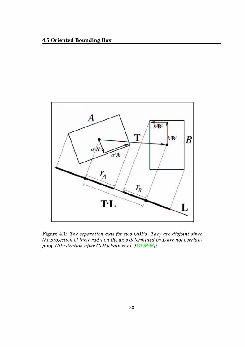
4.3 Separating AxisThe separating axis theorem[Got96] is heavily used for fast rejectiontests for convex, disjoint polyhedra. Two polyhedra A and B, thereexists a separating axis where the projections of the polyhedra, whichform intervals on the axis, are also disjoint. If A and B are disjoint,then they can be separated by an axis that is orthogonal to: a face of A,a face of B, or an edge from each polyhedron.

20

4.4 Axis Aligned Bounding Box

4.4 Axis Aligned Bounding BoxAn axis aligned bounding box (AABB), is a box whose faces have nor-mals that coincide with the standard basis axes. AABB is the simplestbounding volume to create. Take the minimum and maximum extentsof the set of polygon vertices along each axis and the AABB is formed.

4.4.1 Building a AABBCreating a AABB bounding volume is very simple. Take the minimumand maximum extents of the set of polygon vertices along each axis andthe AABB is formed.

4.4.2 AABB Intersection TestSince the AABB is aligned with the main axis directions there is suffi-cient to decribe the volume with two points. A Simple test is decribedbelow:tab [ ] = [ x , y , z ] ;for ( int i = 0 ; i < 3 ; i + + ) {

i f ( a_min [ i ] > b_max [ i ] | | b_min [ i ] > a_max[ i ] )return (DISJOINT)

return (OVERLAP)

4.5 Oriented Bounding BoxAn oriented bounding box (OBB) is a rectangular bounding box with anarbitrary orientation in space. It is an AABB that is arbitrary rotatedto fit the volume as best as possible.

4.5.1 Building an OBBGottschalk et al.[GLM96] showed that a tight-fitting OBB enclosing anobject can be found by computing an orientation from the triangles ofthe convex hull.

First we compute the convex hull of all the triangles in the object.If the vertices of the i’th triangle are the points pi,qi, and ri, then areaof the i’th triangle in the convex hull is:

Ai =1

2

∣∣(pi − qi)×(pi − ri

)∣∣

21

4.5 Oriented Bounding Box

Let the surface area of the entire convex hull be denoted by:

AH =∑

i

Ai

Let the centroid of the i’th convex hull triangle be denoted by:

ci =pi + qi + ri

3

Let the centroid of the convex hull, which is a weighted average andthe triangle centroids (the weights are the areas of the triangles), bedenoted by:

cH =

∑iA

ici∑iA

i=

∑iA

ici

AH

Now we can compute a 3 × 3 covariance matrix, C, whose eigen-vectors are the direction vectors:

Cjk =

n∑

i=1

Ai

12AH(9cijc

ik + pijp

ik + qijq

ik + rijr

ik

)− cHj cHk

After computing C the eigenvectors are computed and normalized.Then we project the points of the convex hull onto the eigenvectors tofind the minimum and maximum along each direction. We then usethis to calculate the center and half-length of the OBB.

4.5.2 OBB Intersection DetectionTo check intersection between two OBBs, A and B, a fast algorithm in-troduced by Gottschalk [Got96] that uses the separation axis theorem,and is about an order faster than previuos methods.

The test is done in the coordinate system formed by OBB A’s centerand axes. B is placed relative to A by rotation B and translation T.The half-dimensions (radii) of A and B are ai, and bi, where i = 1, 2, 3.The axes of A and B are the vectors Ai and Bi, for i = 1, 2, 3. These willbe referred as the 6 box axes.

According to the separating axis theorem, it is sufficient to find oneaxis that separates A and B to be sure that they are disjoint. Fifteenaxes has to be tested: Three from the faces of A, three from the faces ofB, and 3 · 3 = 9 from combinations of edges from A and B.

As a consequence of the orthonormality of the matrix A = (A1,A2,A3),the potential separating axes that should be orthogonal to the faces of

22

4.5 Oriented Bounding Box

Figure 4.1: The separation axis for two OBBs. They are disjoint sincethe projection of their radii on the axis determined by L are not overlap-ping. (Illustration after Gottschalk et al. [GLM96])

23

4.6 OBBTree

A are simply the axes A1,A2, and A3. The same holds for B. The re-maining nine potential axes formed by one edge each from both A andB, are then cij = ai × bj.

The centers of each box projects onto the midpoint of its interval.By projecting the box radii onto the axis, and summing the length oftheir images, we obtain the radius of the interval. If the axis is parallelto the unit vector L, then the radius of box A’s interval is:

rA =∑

i

∣∣aiAi · L∣∣

rB =∑

i

∣∣biBi · L∣∣

The placement of the axis is immeterial, so we assume it passesthrough the center of box A. The distance between the midpoints of theintervals is |T · L|. So, the intervals are disjoint if:

|T · L| >∑

i

∣∣aiAi · L∣∣ +∑

i

∣∣biBi · L∣∣

The last step is due to the fact that the columns of the rotationmatrix are also the axes of the frame of B. After simplifying all theterms, this axis test looks like:

|T3R22 −T2R32| > a2 |R32|+ a3 |R22|+ b1 |R13|+ b3 |R11|

4.6 OBBTreeOBBTrees was first presented at SIGGRAPH 96 by Gottschalk et al.[GLM96] with a paper called "OBB-Tree: A Hierarchial Structure forRapid Interference Detection". This paper have strongly influenced fur-ther research on CD algorithms. As the name OBB-Tree algorithm im-plies, the bounding volume used is the oriented bounding box, the OBB.OBBs converge much faster to the underlying geometry they are hold-ing than AABBs (axis-aligned bounding box) and spheres. OBBTreeshave been widely used both in scientific simulations and in games.

4.7 Sweep and PruneThe sweep and prune technique was developed by M. Lin[Lin94] andexploits that objects undergo small changes in their position and ori-entation from frame to frame. Lin proved that the bounding box prob-lem can be solved in O

(n log2 n+ k

)time (where k is the number of

24

4.8 Hierarchical Collision Detection

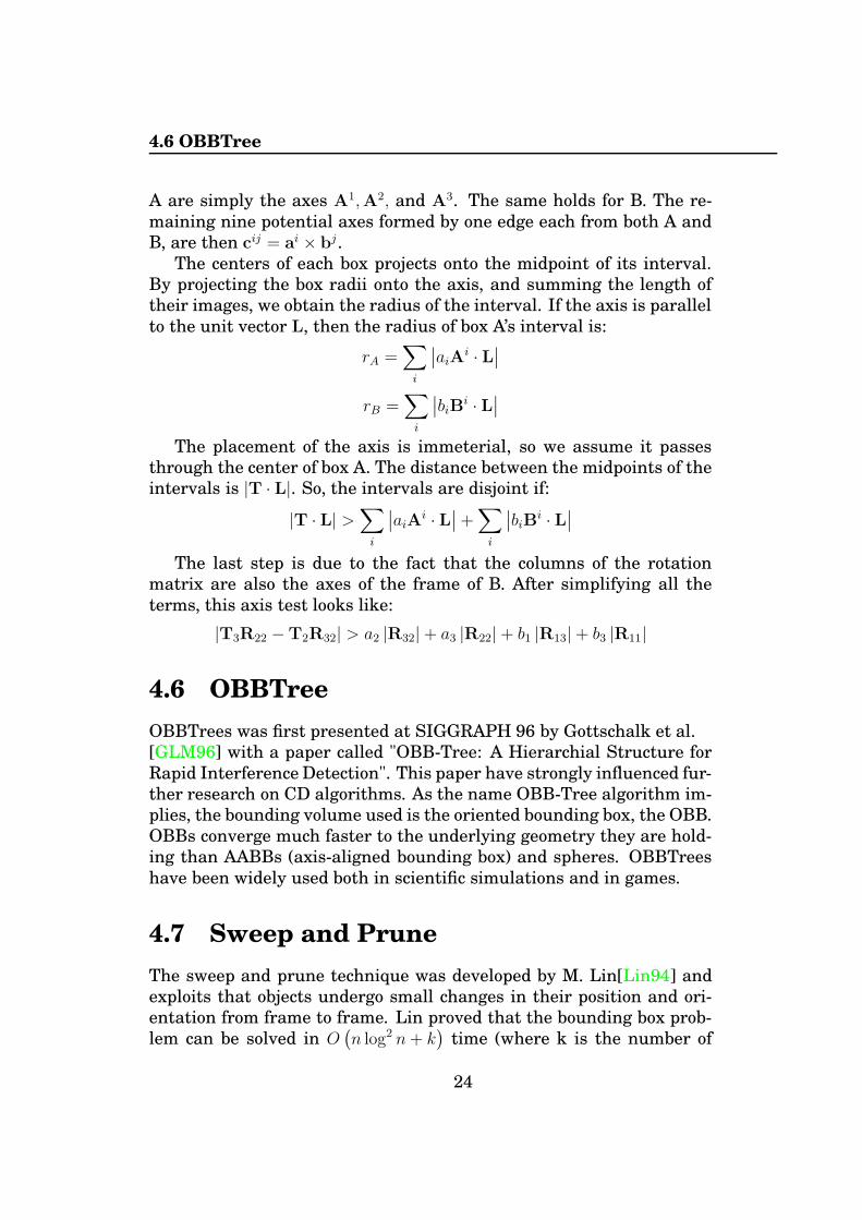
s1 e1 s2 s3 e2 e3

Figure 4.2: Graphical view of Sweep-and-prune for one axis. When s3 isencountered s2 is already in the active list. There is an overlap betweenbody 2 and 3 in at least one axis.

pairwise overlaps), but it can be improved by exploiting coherence andso be reduced to O (n+ k).

If two AABBs overlap, then all three one-dimensional intervals ineach axis direction must also overlap. Start and endpoints of the AABBsin each axis is stored in three lists, these values are stored in increas-ing order. This list is then swept from start to end. When a startpointis found it is stored in a active list. When its endpoint is found it is re-moved from the active list. If another start or endpoint is encounteredwhen the startpoint is in the active list we have overlap. A graphicalexample of how sweep and prune works is shown in figure 4.2.

This procedure would take O (n logn) to sort all the intervals, plusO (n) to sweep the list, and O (k) to report overlapping intervals. Butsince the lists are not expected to change very much from frame toframe, a bubble sort or insertion sort can be used with great efficiencyafter the first pass has taken place. It was shown in[SH76] that thesesorting algorithms sort nearly-sorted lists in an expected time of O (n).

4.8 Hierarchical Collision DetectionA hierarchy that is commonly used in the case of collision detectionalgorithms is a data structure called a k-ary tree, where each node mayat most have k children. Most algorithms use k = 2, a binary tree. Theroot node is a BV that encloses the whole object. Each internal nodeenclose all of its children in its volume, and at each leaf, there are one

25

4.9 Collision Report

or more primitives.There are three ways of creating a hierarchy: a bottom − up, top −

down, and a incrementaltree − insertion.The bottom-up method start with creating a BV for each primitive

and then merge two and two nodes that are close in proximity togetherewith a parent node until there are only one root node left.

The incremental tree-insertion method starts with an empty tree.Then all other primitives and their BVs are added one at a time to thistree.

The top-down approach is the method that is most frequently used.It starts by finding a BV for all the primitives to the object which is theroot of the tree. Then a divide-and-conquer method is applied wherethe BVs is split into two (or k) parts. There is then created a BV basedon the primitives in each part. This metod is followed until there areonly one primitive left in each part.

The big challenge is to find a satisfactory bounding volume and ahierarchy construction method that create balanced and efficient trees.

4.9 Collision ReportTo make the collision detection routine useful there must be a way toget some confirmation that overlap is found. The most easy solution isto just return a boolean that say if there are any overlaps or not. Thisworks for many situations, but since we want to use it in a rigid bodysimulation this is not sufficient. To simulate contacts in a rigid bodysimulation we minimum need the contact point and contact normal.This is more thoroughly explained in chapter 7.

To find the contact point and contact normal has an enormous neg-ative impact on performance, but there is no way around it. Furtherdiscussion is found in the implementation section 5.2

26

Chapter 5

Collision DetectionImplementation

When deciding which CD algorithm to use I wanted a better solutionthan the first one Trond Gaarder and I wrote in Jan 2002. That wasan object specific algorithm which used simple geometry observationsto check for collisions. It worked well for spheres and simple surfaces,but when adding cubes and thetrahedrons it took too much resourcesand was not usable.

A new implementation of a collision detection routine had to aviodthe problems that were encountered in the previous attempt. A set ofrequirements were set to avoid earlier problems.

Requirements

• Generic collision detection algorithm. To be flexible, the CD al-gorithm can not be object specific. This means we should checkfor collisions on a triangle level.

• Fast. Since there will be a lot of computations regarding the rigidbody simulation it is desirable that the CD algorithm use as littleCPU time as possible.

• Not too complex. Since the timeframe of the thesis is limited, andthe focus should mostly be on rigid body simulation it must bepossible to implement it within a timeframe of 6-9 months.

BSPTrees [FKN80] was considered since its widely used especiallyin computer games. The problem with BSPTree is that it generates itscollision tree from the user position and camera direction. This works

27

5.1 Implementation of OBBTree

very well in FPS (first person shooter) games, but not when doing sim-ulations.

Other techniques that caches withnesses like V-Clip[Mir98], wasnot chosen because these are generally more complicated than bound-ary representation techniques.

The decision fell on OBBTrees. The OBBTree design is clean andnot too complex. The algorithm is widely accepted as one of the fastesaround. It has been criticised to use too much memory, but since wewould not generally simulate with models with more than +20K of tri-angles this was not a big issue.

The OBB algorithm performs very well when deciding overlap betweenobjects that are close in proximity, but is quite costly to check for over-lap on every object in the simulation. What we also want is an al-gorithm that quickly can determine if two boundary repersentationsoverlap.If they do, we can then further check for overlap with the OBBalgorithm.

The Sweep-and-Prune algorithm is perfect for this, and is used justfor this purpose in some CD packages. Sweep-and-Prune is easy tounderstand, but difficult to implement. Even so, the sweep-and-prunealgorithm will speed up the collision detection dramatically so it shouldtherefore be implemented.

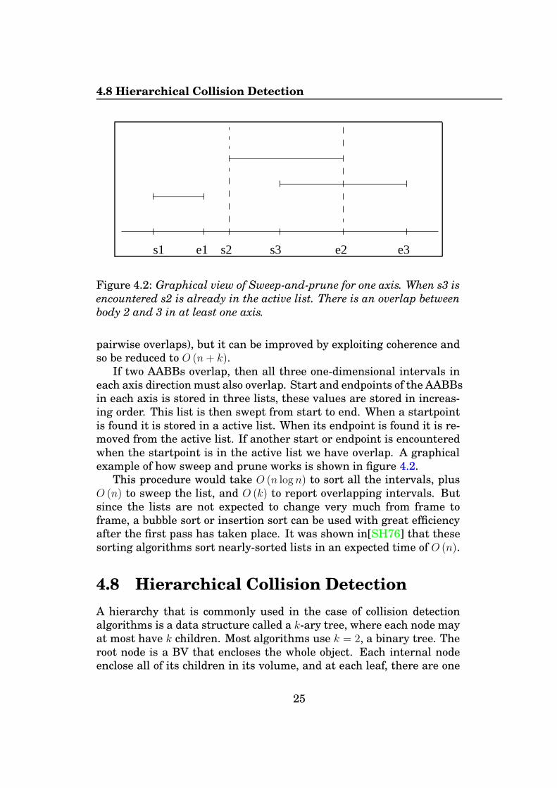
Figure 5.1 show the outline of the collision detection routine andhow it is integrated with the rigid body simulator. The collision routinewas upon creation called Java Axis-aligned Object-oriented Collision-detection (JAOC).

5.1 Implementation of OBBTreeAn OBBTree need tree nodes that can be used to rapidly check for over-lap and either discard it if it is disjoint or call its children to finallycheck triangle-triangle if it overlap. The node need to specify the rota-tion and translation based on its parent and a size. If it is a leaf node italso has a pointer to the triangle it is bounding. If it is not a leaf nodeit has pointers to two child nodes. One in the positive and one in thenegative direction based on its center.

To generate the tree a triangle array is given to the root node, itcalculates the translation and rotation of the OBB box that contain allthe triangles. When there are more than one triangle in the trianglearray a recursive method that calculates the translation and rotation

28

5.1 Implementation of OBBTree

Sweep−and−Prune

Exact Collision Detection

OBBTree Simulation

Overlapping pairs

Colliding pairs

Collision Response

Object Transformations

Figure 5.1: Diagram of the collision detection system.

of its children is called. The triangle array is divided in two new ar-rays with respect of the OBB node’s center and the mean point to thetriangles. The new arrays are now used when calculating the childrensattributes until the length of the array is 1. With this in mind we cancreate a OBB node object like this:

class OBBox {

RBDMatrix3d rotat ion ;RBDVector3d translat ion ;RBDVector3d s ize ;

OBBox Pos ;OBBox Neg ;

Triangle3d trp ;}

The Pos, Neg and trp objects are all references.

The calculation of translation and rotation is not an easy task (viewthe theory of generating a OBB tree). Several helper classes are needed,we use a class to help us calculate the areal and covariance matrix ofa triangle. A class to accumulate all these values is also needed. ATriangle class is used for collision detection and generation of the tree.

29

5.2 Collision Report Implementation

To keep track of all the triangles and do collision detection we needa class to hold it all in place, a OBBTree class. The OBBTree containall the geometric data of an object in 3d space. And has methods tocheck for contact with other OBBTrees. It must store the triangle arrayand manage the process of adding triangles to the tree. It also need tostore the rotation and translation values of the whole object. Simplifiedoutline of the OBBTree:class OBBTree {

OBBox root ;Triangle3d t r i s [ ] ;

RBDMatrix3d rotat ion ;RBDVector3d translat ion ;

}

The implementation is more complicated since we need to keep trackof contact pairs, number of contacts, number of triangles, etc.

5.2 Collision Report ImplementationAs mentioned we need the ability to find the contact point and the con-tact normal. Most current implementations only return a boolean in-dicating if two objects overlap. There are some implementations thatfind the triangles that overlap, but no overlap point. There are tworeasons for this, it is difficult to implement and it has a huge perform-ance impact.

One of the requirements of JAOC is that it should not only be usedin rigid body dynamics, but also in other settings.

With this in mind the OBB collision detection routine was imple-mented with two methods that do almost do the same thing, one thatreturn a boolean that indicates if contact is detected and one that findwhich triangles that overlap. The other method have a class calledJAOCContact as a parameter. The contact point and contact normal isstored in this class. JAOCContact is shown here:public class JAOCContact {

private int bodyA ; // body containing ver t ex pointprivate int bodyB ; // body containing faceprivate RBDVector3d contact ; // contact point in world coordprivate RBDVector3d normal ; // contact normal

30

5.3 Implementation of Sweep and Prune

private RBDVector3d edgeA ; // direc t i on of Aprivate RBDVector3d edgeB ; // direc t i on of Bprivate boolean vf ; // true i f ve r t ex/face contact

}

A contact has a reference to the bodies and a contact point. This pointis given in world coordinates. A contact normal is also calculated, ifthe contact is a vertex/face contact, the contact normal is the normalof the face. If it is a edge/edge contact, the normal is given as thecross product of the two contact edges. If we have a vertex/face contact,the body that has the contact face is referenced by body B, the vertexpoint by body A. This make it easier to calculate an apply the impulseon the two bodies. The JAOCContact class stores the values we needto calculate the contact forces between the bodies. In chapter 6 theproblem of calculating and appling the forces to the bodies is discussed.

5.3 Implementation of Sweep and PruneThe sweep and prune routine has references to all the objects in thesimulation. When a object is loaded, the triangles are added to a AABBobject which again has a reference to a OBBTree.

The AABB generates the tree upon initialization and is added to aAABB manager. The AABB manager has a list of all the AABB ob-jects and a three dimensional list where the end and start points of theAABB in each direction are stored. Before the simulation starts the listis sorted. During simulation the three dimensional list is sweept andprunes as described earlier. When an overlap in all three dimensions isfound the AABB collision pair more accurately check for overlap withthe OBB routine.

If an overlap is found, it is reported to a list of overlapping pairswith object identifiers of the AABB’s and the collision point. The list ofoverlapping pairs are later used by the physics routine to calculate thecollision forces and reactions.

public class JAOCManager {

// pointers to the three linked l i s t s , one for each axisprivate EndPoint sweepList [ ] ;

// AABBObjects pointers to a dynamic array of pointers .private JAOCObject AABBObjects [ ] ;

31

5.4 Performance

// overlappingPairs contain a l l the pair o f// AABBObjects that overlap . This l i s t i s used// by the OBB c o l l i s i o n de t e c t i on routine .public JAOCAABBCollisionReport overlappingPairs ;

// a l l contacts reported by the OBB routinepublic JAOCContactManager contacts ;

}

The variable sweepList is a three linked list that contain the startand end point of the AABB’s in each axis. It is this list that is sweept foreach timestep to check for overlap. All overlaps are added to JAOCAAB-BCollisionReport object. The overlapping objects are kept in the listuntil the routine report them not to be overlapping. It is caching theoverlaps from previous timestep, so already reported overlaps are notreported, only new and previously overlapping pair that do not longeroverlap.

For each timestep the list of overlapping pairs is more accuratelychecked for overlap by the OBB routine. All overlapping pairs thatare found by the OBB routine are added to the JAOCContactManagerobject that goes through the list and calculate the new constraints.Chapter 7 Contact, describes how contacts are handled in rigid bodydynamics.

5.4 PerformanceJAOC was written to be used in rigid body dynamics, but it can be usedin anything from robotics, CAD design and games. The only require-ments are that the objects must be specified by triangles and trianglepoints do not change position with respect to another during the simu-lation.

JAOC have different collision detection options buildt into it. It hastwo different methods of finding contacts. It can find the exact contactpoint and contact normal, or find the overlapping triangles without anyspecified contact point.

JAOC can also be set to only find the first overlap between twoobjects. This function can be used with the exact collision detectionmethod or the overlapping triangle method. These options have a bigimpact on performance. The fastest is when JAOC is set to only findthe first contact and the overlapping triangles. The slowest is when wewant to find all contacts, their contact point and their contact normal.

32

5.4 Performance

It is difficult to measure the performance of collision detection routinesand implementations since the routines are written with different designsand purposes.

Some different designs and purposes are listed here:

• Handle complex topology

• Highly accurate collision detection

• Handle many objects

• Handle deformation of objects during simulation

All these different designs make it difficult to compare different col-lision detection routines. The best way to test performance is to test itin a setting which would be representative for what the routine werebuilt for.

5.4.1 Demo TestThe demo test was run on a Pentium 4, 2.4Ghz with 768mb RAM, run-ning Debian Linux. All tests used the latest version of Java SDK,1.4.2. The demo program test two torus objects which move througheachother. Each torus has 5000 triangles. All different options regard-ing contact report and number of contacts were tested.

• Finding all overlapping triangles: Average 8-10 overlaps foundfor each millisecond.

• Finding all overlapping triangles and the exact contact point andnormal: Average 7-9 overlaps found for each millisecond.

• Finding the first overlapping triangle: Average time is 1-3 milli-seconds.

• Finding the first overlapping triangle and the exact contact pointand normal: Average time is 1-3 milliseconds.

When large objects are totally overlapping or close to a completeoverlap there are very many reported contacts and the routine has tocheck almost every leaf node for overlap. This reduces JAOC’s per-formance since checking all leaf nodes for overlap is costly. Since thereare no interpenetration during rigid body simulation this is not a bigproblem. When large objects are in close proximity without contact or

33

5.4 Performance

when in contact, the JAOC performes very well. However there is aflipside, the demo test use 174MB of memory. This is more than ex-pected, but it must be noted that the test was using double precisionnumbers. When using single precision numbers the memory footprintwould be much smaller.

However the OBB routine is known to use a lot of memory. Eachnode stores the translation, rotation and size of the bounding volume.The node also have pointers to two child nodes and each leaf node hasa pointer to a triangle. When we have N triangles there are 2 × N − 1nodes in the OBBTree. This is the main reason of the high memoryusage, but there are some solutions to this problem.

5.4.2 OptimizationDuring the implementation of JAOC several new ideas of improve-ments have emerged, the best and probably most memory efficient ideais described here:

Each leaf node in the OBBTree object is a OBB node which has areference to a triangle. During the recursive collision queries, whenchecking two leaf nodes for overlap, the pair of bounding volumes ischecked for overlap. Then, only if the OBB overlap, the triangles arechecked for exact intersection. The idea is to simply skip the the firstbounding volume test, and directly perform the triangle overlap testinstead. A triangle-triangle overlap test is almost as fast as a OBB-OBB overlap test. Skipping the OBB-OBB test for leaf nodes should beefficient because:

• If the triangles overlap, we would have to perform the triangleoverlap test anyway. In this case the OBB-OBB test prior to thetriangle-triangle test can be skipped.

• If the triangle do not overlap the the test is roughly as fast asthe OBB-OBB overlap test. There is also the possibility that theOBB-OBB test report overlap but the triangle-triangle overlaptest would show that there are no overlap.

Does this mean that OBB nodes are not needed in leaf nodes any-more? No, because we still may have to collide a leaf node against ainternal one. This mean that we need a triangle-OBB overlap test. As-suming we have this routine, we can remove the leaf nodes altogether

34

5.4 Performance

by storing the triangles in the parent nodes, replacing previous point-ers to the leaf nodes we just discarded.

This reduces memory consumption considerably, instead of having2×N−1 nodes, we now have N−1 nodes. Moreover, replacing the OBB-OBB test with a more accurate triangle-OBB test actually leads to lesstests since the OBB-OBB can report overlap wheras the triangle-OBBtest does not.

The required triangle-box test has been derived by Tomas Akenine-Möller[AM01], and turns out to be roughly as fast as the standardOBB-OBB test.

With these improvements on the existing implementation it woulduse much less memory and be somewhat faster.

Another less drastic memory improvement would be to use qua-ternions instead of a 3x3 matrix to represent rotation of the OBB node.Using quaternions results in substancial memory savings, but need 13more operations for each OBB overlap test. This is the usual trade ofbetween memory and CPU time.

5.4.3 ConclusionJAOC performes very well with large and small objects, objects thatare in close proximity and objects that are far away. It has differentmethods of reporting contacts which makes it usable by many differ-ent applications. The problem is that the memory usage is high. Butwith the implementation of the ideas above the memory usage wouldbe drastically reduced.

35

Chapter 6

Rigid Body Library

The development of the rigid body library has undergone serveral phasesand changes. The requirements were set very early, and have notchanged much during the development.

Requirements

• Use a modular architecture

• The architecture should be flexible and easily reusable. The basiccomponents should be easily usable for different rendering en-gines.

• It should be suitable for interactive animations. This means speedis important, but not of the cost of extendibility and the modulararchitecture (see 1,2). This means accuracy may be sacrificed inexchange for more speed (if neccessary).

• The dynamics system should not be purely impulse-driven, butsupport forces on the bodies.

• The numerical solvers used to solve the differential equationsmust prevent numerical drift.

• Implementation of collision detection and handling.

• Model friction.

• User manual for the library

• Examples of possible applications/demos/games using the library

36

6.1 Implementation

6.1 ImplementationOne of the goals of this library was that is should be easily reusableand extendable. The libraries have been written in an object orientedway. It could have been written without objects, but a modular andeasily extensible library was one of the goals of this project. The libraryhas been separated into three parts; Math, collision detection and rigidbody simulation.

Math Library

The math library extends the existent vecmath library from SUN whichis a part of Java3D[Mic97]. The vecmath library was chosen so ourapplication could easily use Java3D as a visualization platform. Thevecmath library is provided so that users who do not want to use thelibrary against Java3D could easily do so. The math library is smallwith the classes RBDVector3*, RBDMatrix3* and RBDQuat4*. Thereare double and single precision version of the classes. Utility methodsfor finding eigenvectors and eigenvalues from a matrix[PFTV92] andquaternion to matrix calculation are provided to name a few.

Rigid Body Library

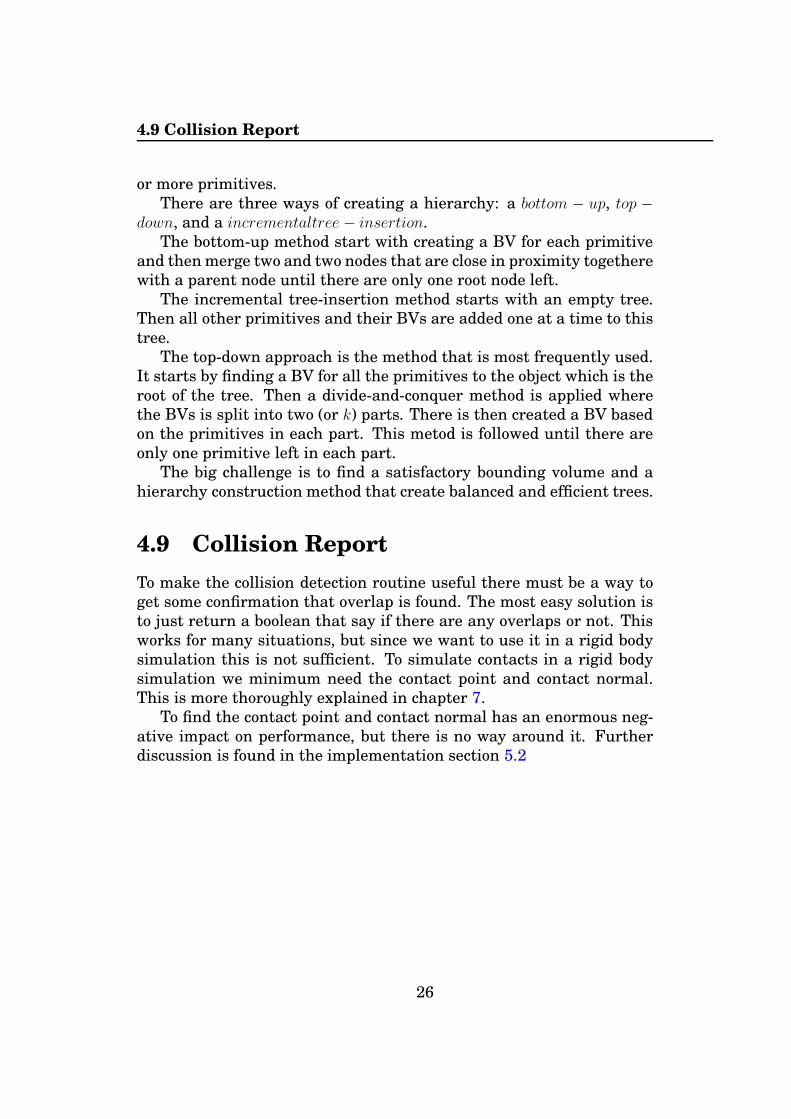
The rigid body library is responsible for the physics and the proper-ties for all objects in the simulation. It has an integrated ODE solverwhich updates position and orientation for each timestep. The ODEsolver could be implemented as a module of its own, but with the ODEintegrated the API could still be clean and it is more efficient. A dia-gram of the rigid body library can be seen in figure 6.1.

Collision Detection Library

The collision detection library is JAOC. JAOC is responsible for detect-ing and reporting contacts. An outline of the library can be found infigure 6.2.

The contact manager works as a connection between JAOC and therigid body module. The issue is where do we apply the contact forceson the objects? It can be implemented in both JAOC and the rigidbody module without much problem. The contact manager is used byboth but it is an integrated part in the JAOC routine. The current

37

6.1 Implementation

Rigid Body SimulatorODE

Calculate new

velocityposition and

New Positions

No OverlapVisualization

CollisionResponse

Overlapping Pair

DetectionCollision

Figure 6.1: Diagram of Rigid body simulator

AABB overlap check (sweep−and−prune)

AABB overlapping pairs

No overlap

OBB overlap check

Simulator

JAOC, Collision Detection

New position

No overlap

Overlap

Figure 6.2: Diagram of JAOC

38

6.1 Implementation

solution is to let the contact manager manage all the physics involvingthe impulse calculations.

Visualization

Java3D is used to visualize the objects, but it is not part of the ri-gid body library nor JAOC. The library is independent of visualizationtechniques and can easily be used by Java3D and GL4Java[Goe01].

6.1.1 Rigid Body LibraryEach body is an object entity in world space and know of nothing otherthan itself. Ideally it should not need to contain any geometric data,just data that is needed to calculate the physical constraints. Withthe use of JAOC as the collision detection library the geometry can bestored in the JAOCObjects and not in the rigid body representation.The basis of a rigid body:

public class RigidBody3D {

// The world coordinate pos i t i on of the bodyprivate MyVector3f pos i t ion ;

// The l inear v e l o c i t y o f the bodyprotected MyVector3f v e l o c i t y ;

// Inverse Mass of the bodyprivate float invMass ;

// The or i en ta t i on of the bodyprivate MyQuat4f or ientat ion ;

// The angular v e l o c i t y o f the bodyprivate MyVector3f omega ;

// The inverse i n e r t i a tensor of the body in body coordinatesprivate MyMatrix3f inert iaInv ;

// Ve loc i t y in body coordinates , used when calculat ing drag e t cprivate MyVector3f bodyVelocity ;

// Linear momentprivate MyVector3f P;

39

6.1 Implementation

// Angular momentprivate MyVector3f L;

// Res t i tu t i on of body ,// say how much energy i s _ l o s t _ during c o l l i s i o nprivate float RESTITUTION;

}

The values of the rigid body object has been explained earlier in thisthesis, so it is not covered here. The inertia tensor is not calculatedby the object and must be calculated before object creation. A staticutility class is provided to easily calculate the inertia tensor for mostcommon geometric objects. The rigid body object stores the inverseinertia tensor instead of the tensor itself. All calculations involving theintertia tensor use the inverse. Therefore there is no reason to storethe actual inertia tensor.

Other initial conditions for each rigid body is specified by assign-ing values to mass, position, orientation, linear moment and angularmoment.

Mass is also a value we use the inverse instead of the value itself.This is mainly because it gives us the possibility to create bodies withinfinite mass, eg. bodies that are stationary in the simulation.

6.1.2 Collision Detection LibraryHere we will assume that JAOC detects all contacts between bodiesand reports it in a decent way. All contacts are stored in a list in theJAOCContactManager class. A contact is stored in the JAOCContactclass. JAOCContact:

class JAOCContact {

private int bodyA ; // body containing ver t ex pointprivate int bodyB ; // body containing faceprivate RBDVector3d contact ; // in world coordinates ;private RBDVector3d normal ; // contact normalprivate RBDVector3d edgeA ; // direc t i on of Aprivate RBDVector3d edgeB ; // direc t i on of Bprivate boolean vf ; // true i f ve r t ex/face contact

}

The JAOCContactManager store all JAOCContacts:

40

6.1 Implementation

public class JAOCContactManager {

private JAOCContact contacts [ ] ;private int numContacts ;

public JAOCContactManager ( ) {}public void addContact ( JAOCContact newContact ) {}

public JAOCContact getContact ( int i ) {}

}

The rigid body objects are stored in two different arrays. JAOCMan-ager store the geometric values and RigidBodyManager store all thephysic values. Now where should all the contacts be processed?

The JAOCContact object contain contact point and contact normal,but only the ids of the contact pair. It also need the rigid body objects.The contact processing could be implemented in the simulator, JAOC oreven in a separate module. It was decided that the contact processingroutine should be a part of the RigidBodyManager. For each timestepthe simulator will give the RigidBodyManager the list of contacts toprocess from JAOCManager.

6.1.3 Rigid Body ManagerThe rigid body manager controls all the bodies. It updates the timestepand calculate new velocities and positions with the use of an ODE. Itis also responsible for the contact computation. A simple outline of theRigidBodyManager:

public class RigidBodyManager {

private RigidBody3D bodies [ ] ;

public RigidBodyManager ( ) {}

public void addBody ( RigidBody3D body ) {}

public void processContacts ( JAOCContactManager contacts ) {

41

6.1 Implementation

}}

To processContacts the JAOCContactManger object is given by the Sim-ulator.

6.1.4 SimulatorThe simulator is the main object in the simulation. It works as a con-nector between the collision manager and the rigid body manager. Foreach timestep it prune the contact manager for all contacts and send itto the rigid body manager that calculate the contact data.

All objects that is simulated has to be added to the simulator. Thesimulator pass the objects to the RigidBodyManager and JAOCMan-ager.

public class Simulator {

public RigidBodyManager rigidBody ;

public JAOCManager jaoc ;

public Simulator ( boolean f i rs tContact , boolean exactOverlap ) {}

public void newObject ( ) {}// add physics data to the current o b j e c tpublic void addRigidBody ( RigidBody3D body ) {}// add a tr iang l e to the current o b j e c tpublic void addTri ( RBDVector3d v1 , RBDVector3d v2 , RBDVector3d v3 ,

int t r i I d ) {}

public void update ( ) {}

}

The booleans given to the constructor is further given to the JAOC-Manager constructor and set what kind of collision detection that willbe used.

The update function updates the timestep and calls the RigidBody-Manager which updates all the state variable of the rigid bodies. Then

42

6.2 Example of Use

the new positions and orientations is given to the JAOCManager andit checks for overlap. If any overlaps is found the JAOCContactMan-ager object is given to the RigidBodyManager which processes all thecontacts.

6.2 Example of UseThis is a small example of how the library could be used to perform arigid body simulation.import org . r ig idbodyl ibrary . math . * ;import org . r ig idbodyl ibrary . jaoc . * ;import org . r ig idbodyl ibrary . rbd . * ;

public class SimulatorTest {

public static void main( String [ ] args ) {

// crea t e the simulator o b j e c tSimulator sim = new Simulator ( false , true ) ;

//use a rig id body u t i l o b j e c t to c r ea t e a box and//add i t to the simulator .BodyCreatorUtil bodyUtil = new BodyCreatorUtil ( ) ;// crea t e a box with width = height = length = 1 and mass 1 0 .// I t s pos i t i on in world coordinate system i s 2 , 0 , 0 .int id1 = bodyUtil . newBox ( 1 , 1 , 1 , 1 0 ,

new RBDVector3d ( 2 , 0 , 0 ) , sim ) ;int id2 = bodyUtil . newBox ( 1 , 1 , 1 , 1 0 ,

new RBDVector3d ( 0 , 0 , 0 ) , sim ) ;// give one of the bodies a l i t t e powersim . getBody ( id2 ) . addForces (

new RBDVector3f ( 2 . 0 f , 0 . 0 f , 0 . 0 f ) , 1 . 0 f ) ;// then give the body a l i t t l e spinRBDVector3f o = new RBDVector3f(−1.0 f , −2.0 f , 0 . 0 f ) ;o . scale ( ( float )Math . sin ( 0 . 5 ) ) ;o . normalize ( ) ;sim . getBody ( id2 ) . setOrientation (

new RBDQuat4f( o . x , o . y , o . z , ( float )Math . cos ( 0 . 5 ) ) ) ;

// do the simulationwhile ( true ) {

sim . update ( ) ;

43

6.3 Summary

}

}}

With utility classes as BodyCreatorUtil it is very easy to add bodies tothe simulation. However it is not difficult to create a custom object.Only pass the triangles to the simulation manually with the addTrimethod.

The example above do not handle graphics, but that does not meanit is difficult to implement it. In the loop that call the update function,the position and orientation of the objects can be retrieved and used bythe graphics objects. The objects can be created by the triangles addedto the JAOCManager.

6.3 SummaryWith a generic collision detection routine and proper contact handlingimplemented it is much easier to simulate rigid body dynamics. Sinceall bodies are objects entities it is very easy to add them to the simula-tion.

44

Chapter 7

Contact

In chapter 2 we introduced the equation of motion for a rigid body.When bodies are in contact we need to prevent them from inter-penetrate.

Lets consider a situation where a cube is falling onto a fixed floor.Since we are dealing with rigid bodies that are non-flexible, we dontwant any inter-penetration at all. This means that at the instant thecube comes in contact with the floor, we must change the velocity of thecube.

Since we treat the bodies as totally rigid, the velocity has to be hal-ted instantaneously to avoid inter-penetration.

This means we have two types of contact to deal with. When twobodies are in contact at some point p, and they have a velocity towardseachother, this is called colliding contact. Colliding contact requires aninstantaneously change in velocity. When two bodies are in contact atsome point p, but the velocity between them are zero we say that thebodies are in resting contact.

In this chapter we will only look at what we do when we have foundand reported a possible collision. A more indepth look at collison de-tection algorithms and some implementations are found in chapter 4,Collision Detection.

7.1 Colliding ContactContacts between polyhedra is either vertex/face contacts or edge/edgecontacts. A vertex/face contact is when a vertex on one polyhedra is incontact with a face on another polyhedra. An edge/edge contact is whentwo edges contact; it is assumed that the two edges are not collinear.

45

7.1 Colliding Contact

For now, we will assume that the contact is frictionless and that theline of action of the impulse is normal to the surface of both objects.When we have a vertex/face contact, we use the normal to the face asthe contact normal. When we have a edge/edge contact, we use the unitvector for each edge and compute the cross product between them, anduse this vector as the contact normal.

Lets say we have got a contact point p, from the collision detectionalgorithm. The contact point is given in world space. We have twobodies A and B.

pa(t) is the point on body A that satisfies pa(t) = p. Similary, wehave the point pb(t) for body B. Even though pa(t) and pb(t) are similarthey do not have the same velocity. The velocity to pa(t) is given by:

pa(t) = va(t) + ωa(t)× (pa(t)− xa(t))

where va(t) is the linear and ωa(t) angular velocity for body A. xa(t) isthe position of center of mass in world coordinates. Similar for B:

pb(t) = vb(t) + ωb(t)× (pb(t)− xb(t))

Now we need to calculate the relative velocity between body A andB. To get the relative velocity we use the contact normal:

vrel = n(t) · (pa(t)− pb(t))

vrel is a scalar and describes the velocity between the two objects. Ifvrel is positive this means that the relative velocity at the contact pointis in the positive n(t) direction and the bodies are moving apart. If therelative velocit is zero the bodies are neither colliding nor separating,they are resting. If the relative velocity is less than zero the bodies arecolliding. If the relative velocity is less than zero we need to stop thebodies from penetrating.

The most obvious thing to do is to apply a force to both objects,but a force will not stop the bodies from penetrating because a forcecan not instantaneously change the velocity. Instead of using force weintroduce a new quantity J , called an impulse [MC95]. An impulseis a vector quantity, like a force, but it has its units of momentum.An impulse can be seen as a huge force integrated over a short periodof time. We think of the time as infinitly small and the force almostinfinitly large. As the force change the momentum over time, a impulsechange the momentum instantaneously.

46

7.1 Colliding Contact

The collision model we will use is called "Newton’s Law of Restitu-tion for Instantaneous Collisions with No Friction." The impulse canbe denoted as:

F∆t = J

Where F → inf and ∆t→ 0.When two bodies collide, an impulse is applied between them to

change their velocity. For frictionless bodies, the direction of the im-pulse will be in the normal direction, n(t). We can write the impulse Jas:

J = jn(t)

Where j is an scalar that gives the magnitude of the impulse. Wewill adopt the convension that the impulse J acts positively on body A,+jn(t), while body B is subject to: −jn(t). Here the collision normal isthe normal computed from the face of body B if it was an edge-vertexcontact or with the cross product if it was an edge-edge collision.

Newton’s Law of Restitution introduces yet another quantity, thecoefficient of restitution, denoted by e or ε. ε must satisfy 0 ≤ ε ≤ 1.The coefficient of restitution tells us how much of the incoming energyis lost during the collision. If ε = 1, no kinetic energy is lost. If ε = 0all kinetic energy is lost and the two bodies will be at resting contactat the contact point.

v+rel = −εv−rel

where v+rel is the relative velocity after the impulse has been applied,

and v−rel is before the impulse has been applied.We further denote v− and ω− as the velocities before the impulse

has been applied and v+ and ω+ are the velocities after the impulsehas been applied. We can now write the velocity after impulse for bodyA as:

p+a (t) = v+

a (t) + ω+a (t)× r

Where r = p− x(t).We can split up the two velocities to:

v+a (t) = v−a +

jn(t)

Ma

where Ma is the mass of body A.

ω+a = ω−a (t) + I−1

a (t) (ra × jn(t))

and I−1a is the inerta tensor of body A.

47

7.2 Resting Contact

After solving for j we get:

j =− (1 + ε) v−rel

1Ma

+ 1Mb

+ n (t) · (I−1a (t) (ra × n (t)))× ra + n (t) ·

(I−1b (t) (rb × n (t))

)× rb

When we have calculated j we plug it in the equation and we havea collision response with the correct spin based on their incoming velo-cities and mass.

7.2 Resting ContactSolving resting contact is hard because the only known methods ofdealing with resting contact demands some sophisticated numericalsoftware, known as quadratic solver.

Let us now say that we have n contact points, and all points arein resting contact. In other words the relative velocity vrel, is zero orsmaller than a numerical threshold. As with colliding contact, we havea contact force that acts normal to the contact surface. With collidingcontact we had an impulse jn(t) where j was an unknown scalar. Forresting contact, there is some force fini(t) at each contact point wherefi is an unknown scalar and ni(t) is the contact normal at the i’th con-tact point. What we want is to determine the value of all the fi’s. Todetermine the value they must all be calculated at the same time, sincethe force at the ith contact point may influence one or both of the bodiesof the j contact point.

When calculating fi we have three conditions. The contact forcesmust prevent inter-penetration, that is, the contact forces must bestrong enough to prevent the two bodies from being pushed "towards"eachother. Second, we do not want the force to act like a "glue" andhold the bodies together. Third, we want the force at a contact point tobecome zero if the bodies begin to separate.

The first condition, prevent inter-penetration. For each contact pointwe use a expression di(t) which describes the distance between two bod-ies at contact point i. If di(t) is negative we have inter-penetration andif it is positive the bodies have broken apart. When the bodies are incontact we have di(t) = 0 (within numerical tolerances) for each contactpoint.

At a contact point i between two bodies A and B, we can construct afunction for di(t):

di(t) = ni(t)× (pa(t)− pb(t))

48

7.2 Resting Contact

The same function can be used with edge/edge contacts since ni(t) pointsoutwars from B towards A. At a contact point we have di(t) = 0, whatwe need it to keep di(t) from decreasing at time t. This means we havedi(t) > 0.

di(t) = ni(t)× (pa(t)− pb(t)) + ni(t)× (pa(t)− pb(t))

di(t) describes the separation velocity at time t. This is exactly what wecalled vrel earlier. For resting contact we know that di(t) is zero, becausethe bodies are neither moving towards or away from eachother at thecontactpoint. What we want to take a closer look at is di(t). When wedifferentiate the equation above we get:

di(t) = ni(t)× (pa(t)− pb(t)) + 2ni(t)× (pa(t)− pb(t)) +ni(t)× (pa(t)− pb(t))

Since pa(t) = pb(t), we can write di(t) as:

di(t) = ni(t)× (pa(t)− pb(t)) + 2ni(t)× (pa(t)− pb(t))

The value of di(t) describes how the two bodies are accelerating to-wards each other at the contact point. If di(t) is positive the bodies aremoving apart, if di(t) = 0 the contact remains. A negative di(t) must beavoided. We have now the constraint

di(t) ≥ 0

for each contact point.The second constraint is simply that fi must be positive. This since

a force fini(t) acts on body A, and ni(t) is the outwards pointing normalof B.

The third say that fi must be zero if contact is breaking. We canexpress this as

fidi(t) = 0

To find all the fi which satisfy the three conditions, we can expresseach di(t) as a function of the unknown fi. We can write each di(t) as

di(t) = ai1f1 + ai2f2 + · · ·+ ainfn + bi

We can write this with matrix syntax

d1(t)...

dn(t)

= A

f1...fn

+

b1...bn

49

7.3 Implementation of Colliding Contact

where A is the n× n matrix of the aij coefficients.

n∑

i=1

fnii(t)dni(t) = 0

can now be written asfTa = 0

We can now write the linear relation as:

a = Af + b

We can now write the three constraints as:

Af + b ≥ 0

f ≥ 0

fT (Af + b) = 0

(7.1)

This is a LCP (Linear Complemtary Problem)[Bar94]. Since we ig-nore friction the matrix A is a PSD matrix. This means that there is asolution to the LCP. The problem is that LCP is NP hard. This meansthat the more contacts we have the solvingtime will increase exeption-ally.

7.3 Implementation of Colliding ContactWhen we have colliding contact, we are given several values from thecollision detection routine. We have a reference to the two colliding ob-jects and the contact point and contact normal. First we need do checkif the the relative velocity vrel between the bodies is zero or smallerthan a numerical threshold. The body object have a method that cal-culate the velocity of a point in the body. A method to check for contactcan then easily be written as:

public int calcRelat iveVel ( ) {re la t iveVe loc i t y . sub ( bodyA . getPointVeloc i ty ( c o l l i s i o n P o i n t ) ,

bodyB . getPointVeloc i ty ( c o l l i s i o n P o i n t ) ) ;int vrel = col l is ionNormal . dot ( re la t iveVe loc i t y ) ;

50

7.3 Implementation of Colliding Contact

i f ( vre l > THRESHOLD) // moving awayreturn NO_COLLISION;

else i f ( vre l > − THRESHOLD) // res t ing contactreturn COLLISION; // t r e a t i t as a c o l l i s i o n

elsereturn COLLISION;

}

When a collision is confirmed by the relative velocity we need tofind the impulse, J = jn(t). We already have the contact normal, butwe need to calculate j. j is defined to be:

j =− (1 + ε) v−rel

1Ma

+ 1Mb

+ n (t) · (I−1a (t) (ra × n (t)))× ra + n (t) ·

(I−1b (t) (rb × n (t))

)× rb

Calculation of j is, though lengthy, quite easy and will not be shownhere, but rather a the method used to apply the impulses on the bodiesas:

public void applyImpulseNoFriction ( ) {MyVector3d J = new MyVector3d ( getCollisionNormal ( i ) ) ;

double j = getImpulse ( ) ; // getImpulse ( ) ca l cu la t e s jJ . scale ( j ) ; // J = n * j ;

bodyA . applyImpulse ( J ) ; // p o s i t i v e impulse on body AJ . negate ( ) ;bodyB . applyImpulse ( J ) ; // negative impulse on body B

}

Since the collision normal is calculated from body B, the positiveimpulse acts on body A, and the negative acts on body B. Then weapply the impulse on the body:

public void applyImpulse ( MyVector3d impulse ) {// Apply the impulse to the bodyP. add ( impulse ) ; // P += impulseMyVector3d tmpVec = new MyVector3d ( ) ;tmpVec . cross ( co l l i s i onPo int , impulse ) ; // L += co l lPo in t X impulseL. add ( tmpVec ) ;

// recompute the auxi l iary variablesv e l o c i t y . scale ( getInverseMass ( ) , P ) ; // v = P / mass

51

7.3 Implementation of Colliding Contact

omega . mul ( getWorldInertiaInverse ( ) , L ) ; // omega = Iinv * L}

When the impulse is added the collision response routine is finishedand the control is given to the simulator.

52

Chapter 8

Java

In this section we will briefly look at the programming language Java,and give an overview of the concepts involved.

8.1 OverviewJava is a relatively new programming languange. It was first releasedin 95 by SUN Microsystems and is still developed further. TraditionalJava applications are applications that are written in Java and thencompiled into byte code form - called Java byte code. This byte codecan be executed by a Java virtual machine (JVM) on any platform thatJava supports. This means that the byte code is completely platform in-dependent, and the JVM protects the underlying machine from illegalinstructions and memory access. Java is an imperative object orientedprogramming languange. Its syntax is very similar to C++. The detailsof Java can be found in the Java languange report [GJS00].

8.2 Java Development KitThe Java development kit (JDK) is the name of the official Sun toolkitto produce Java applications. It consists primarily of a compiler, javainterpreter, core API, and the full documentation of the Java core API(javadoc). The latest version of JDK is version 1.4.1 which was releasedin the end of 2002. The official JVM follow the same version numbers.

53

8.3 Java Virtual Machine

8.3 Java Virtual MachineWith each version the speed of Java applications has improved signi-ficantly. Originally JVMs were simply byte code interpreters that ex-ecuted one command after another. With JDK 1.1, Just-in-Time (JIT)compilation was introduced to the virtual machines. These compiledeach class to machine code before the first time it was executed. Thisshould have caused Java programs to become as fast as any staticallycompiled program.

Unfortunately, this was not the case, since traditional compiler tech-nology relies heavily on inlining to gain their high performance. Thiswas not easy in Java because each class in byte code form is completelyindependent of other classes. This flexibility is enhanced even more bythe possibility of dynamically loaded classes. Since each class in JDK1.1 and JDK 1.2 was compiled to machine code one at the time theconsequence was that it was impossible to inline method across classboundaries or even within classes themselves if those methods werenot private.

Several approaches have been used to solve this problem.

• Assume that all classes immediately presented are static and com-pile the classes as they were written in any other statically com-piled languange. This is the approach used by the Java staticcompilers.

• Allow the compiled machine code to be recompiled at run-time ifthe involved set of classes changes. This is the approach used byHotspot virtual machines (JDK 1.3 and later).

8.4 Java HotspotOne of the major innovations on Java is the devolpment of Hotspottechnology (JDK 1.3 and later), a kind of adaptive optimizer technology.[Gos01]

The idea behind this technology is that the application is analyzedat run-time and optimizations are performed based on these results.

The first times some piece of code is run, it is run interpreted, andwhen the system has gathered enough information about the run-timebehavior of the application it aggressively compiles the sections of codethat are run the most; the hotspots.

54

8.5 Java Performance

The idea is that it is better to use much time compiling the code thatis run frequently rather than performing inferior compilation to it allas is usually done by JIT compilers.

This strategy introduces an initial overhead to the application asit start up (the so- called warm up period) while it analyzes run-timebehavior and runs the optimizing compiler.

The optimizations that can be performed on the code can be muchmore aggressive than the optimizations performed with traditional staticcompilers, such as C++ compilers, because the compilation can be un-done and redone at any time. This means that if the general run-timebehavior changes then the machine code can, and probably will alsochange.

In general, the Hotspot virtual machine first attempts to in-line asmuch code as possible. Then the full range of traditional optimizationtechniques is applied to inlined code. Special optimizations for Javaare:

• Array bounds check elimination.

• Elimination of checked type casts.

• Non-final methods (virtual methods) can be turned non-virtual ifthey are not derived or never used polymorphically.

8.5 Java PerformanceFrom being just a simple byte code interpreter to the use of hotspottechnology, Java performance has increased dramatically. The first ver-sion of Java (JDK 1.0), was approximately 20-40 times slower that C++.JDK 1.3 had a factor 0.7 - 4 slower that C++, and JDK 1.4 is from 0.5-3slower than C++. This is based on tests[Mar02] where both the C++and the Java code were tweaked as much as possible. Further, if theprogram uses 3D hardware, as most games today do, most of the ex-ecution time is spent on 3D hardware, which means the performancedifference between Java and C++ becomes even less.

55

8.6 Java3D

8.6 Java3D

8.6.1 BackgroundJava3D, a relatively new 3D API, tries to learn from the existing 3Dgraphics interfaces. It sits somewhere in the middel of the low levelAPIs like OpenGL and high level like VRML [VRM97].Java3D provides a structured scene graph approach to representingobjects in 3D space. On top of this, it provides a system for buildingcustom behaviours that act according to a variety of simulus withinthe API. Java3D also provides a lot of glue capabilities, such as genericinput device support and 3D sound.Java3D exists as part of the Java Media APIs [JMA]. The various APIsin this framework provide the capabilities for integrating with othermultimedia and Internet technologies.In order to provide a decent level of performace, Java3D uses a lot ofnative code provided by the operation system libraries. On a Solarisor Linux based machine, this means making use of OpenGL rendering.MS Windows users may either use OpenGL or Direct3D. Native vodeuse is restricted to only the final rendering steps while most of the corefeatures are written in Java.

8.6.2 Future of Java3DSUN finalized version 1.3 of Java3D in the summer of 2002. Version1.3.1 was released 14 may 2003 which where bugfixes and performanceenhancement.

According to Doug Twilleager a Java3D SUN developer, parallelwith Java3D 1.3.1, Java3D 1.4 will be developed. Some of the newfeatures that are currently being considered are:

• Programmable Shading (Vertex/Pixel Shaders)

• Stencil buffer support

• Limited Extensibility

• Render to texture

The JSR for Java3D 1.4 will be filed by Siggraph (July 21). Ac-cording to Doug Twilleager they will work to provide as a compatibileshader languange with OpenGL2 and DirectX9 as they can.

56

8.6 Java3D

With version 1.4 Java3D will take a leap forward when dealingwith the new graphics hardware possibilities that are only usable withOpenGl and DirectX at the moment.

The OpenGL2 specs also include native Java bindings.

57

Chapter 9

Conclusion

We have presented techniques for constructing a rigid body simulationsystem. We have described an implementation of a system that canbe used for interactive, real-time simulation. We presented differentmethods of collision detection and an implementation of a flexible andpowerful collision detection routine. The flexibilty of the collision de-tection routine make it usable in many different fields. A library isprovided that make it easy to create applications for simulating rigidbody dynamics.

9.1 Progression, Difficult SubjectsWhen the first attempts at creating a object specific collision detectionroutine failed because of poor performance. It was decided that a moresophisticated collision detection routine was needed.The implementation of JAOC was planned to take no more than 6-7months. During development it became clear that the routine was morecomplex than expected and there were several technical problems thattook much time to implement and debug. Some of the challenges were:

• Computation of the OBBTree.

• Calculate the rotation and translation of the OBB nodes

• Overlap check between OBB objects

• Finding exact collision point and normal

The OBB routine was implemented first, and by then we knew thatit would be impossible to finish JAOC within the timeframe we had

58

9.2 Further Work

planned. The OBB routine worked and would be sufficient for ourneeds, but we felt that it was a half-done product and it would be moreusable with the sweep-and-prune routine implemented. It was decidedto finish JAOC as initially planned.

When JAOC was completed we had a collision detection routine thatwas fast, flexible and it could be usable in much more that rigid bodydynamics. It also has an integrated collision handling routine whichmake it very easy to perform contact computation on the objects.

As a result of the time spent on JAOC there were less time spenton the physics part than planned. Resting contact and contact withfriction are the two main subjects that were put aside.

9.2 Further WorkThere are several directions in which this work could be built upon:

• Implementation of resting contact and contact modeling with fric-tion.The theory of resting contact is provided in section 7.2 the maintask would be to create a LCP solver. The implementation withthe existing library would not be complicated.

• Implementation of contact with friction.David Baraff has written a paper[Bar94] where he introduces amethod for solving the problem.

• Further development of the collision detection routine.Some methods of improving JAOC where provided in section 5.4.2.The exact collision detection routine should be rewritten. The al-gorithm for finding exact overlap is slow and it find many duplic-ate contact points.

59

Bibliography

[ABJN85] D. Ayalla, P. Brunet, R. Juan, and I. Navazo. Object Repres-entation by means of Nonminimal Division Quadtrees andOctrees. ACM Transactions of Graphics, 4:41–59, 1985.

[AM01] Tomas Akenine-Möller. Fast 3D Triangle-Box OverlapTesting. Journal of Graphics Tools: JGT, 6(1):29–33, 2001.

[Bar94] David Baraff. Fast contact force computation for nonpenet-rating rigid bodies. Computer Graphics, 28(Annual Confer-ence Series):23–34, 1994.

[BW97] David Baraff and Andrew Witkin. An Introduction to Phys-ically Based Modeling: Rigid Body Simulation I - Uncon-strained Rigid Body Dynamics. Computer Graphics, 1997.

[FKN80] H. Fuchs, Z.M. Kedem, and B.F. Naylor. On Visible SurfaceGeneration by A Priori Tree Structures. Computer Graph-ics (Proceedings of SIGGRAPH 80), pages 124–133, 1980.

[Gal01] P. Galli. Study - Java to overtake C/C++ in 2002. 2001.

[GJK88] E. G. Gilbert, D. W. Johnson, and S. S. Keerthi. A FastProcedure for Computing the Distance between ComplexObjects in Three-Dimensional Space. IEEE Journal of Ro-botics and Automation, pages 193–203, 1988.

[GJS00] J. Gosling, B. Joy, and G. Steele. The Java Languange Spe-cification. Addison-Wesley, second edition, 2000.

[GLM96] S. Gottschalk, M. C. Lin, and D. Manocha. OBBTree: AHierarchical Structure for Rapid Interference Detection.Computer Graphics, 30(Annual Conference Series):171–180, 1996.

[Goe01] Sven Goethel. OpenGL for Java, GL4Java., 2001.

60

BIBLIOGRAPHY

[Gos96] J. Gosling. The Java Languange - an overview. 1996.

[Gos01] J. Gosling. The Hotspot Technology. 2001.

[Got96] S. Gottschalk. Separating axis theorem. Technical ReportTR96-024, Dept. of Computer Science, UNC Chapel Hill,1996.

[Hub96] Phillip M. Hubbard. Approximating Polyhedra withSpheres for Time-critical Collision Detection. ACM Trans-actions of Graphics, 15, 1996.

[JMA] Java Media API.

[KHM+98] J. T. Klosowski, M. Held, J. S. B. Mitchell, H. Sowizral,and K. Zikan. Efficient Collision Detection using Bound-ing Volume Hierarchies of k-DOPs. IEEE Transactions onVisualization and Computer Graphics, 4:21–36, 1998.

[Lin94] Ming Chieh Lin. Efficient Collision Detection for Anima-tion and Robotics. Technical Report ERL-94-13, 1994.

[Mar02] Jacob Marner. Evaluating Java for Game Deveolpment.2002.

[MC95] Brian Mirtich and John F. Canny. Impulse-Based Simu-lation of Rigid Bodies. In Symposium on Interactive 3DGraphics, pages 181–188, 217, 1995.

[Mic97] SUN Microsystems. Java 3D API Collateral, TechnicalWhite Paper, 1997.

[Mir96] Brian Mirtich. Fast and Accurate Computation of Poly-hedral Mass Properties. Journal of Graphics Tools: JGT,1(2):31–50, 1996.

[Mir98] B. Mirtich. Rigid Body Contact: Collision Detection toForce Computation, 1998.

[PFTV92] W. H. Press, B. P. Flannery, S. A. Teukolsky, and W. T. Vet-terling. Numerical Recipies in C: The Art of Scientific Com-puting. Cambridge University Press, 1992.

[SH76] M. Shamos and D. Hoey. Geometric Intersection Problems.Proceedings of the 17th Annual Conference on Foundationsof Computer Science, pages 208–215, 1976.

61

BIBLIOGRAPHY

[van97] Gino van den Bergen. Efficient collision detection of com-plex deformable models using AABB trees. Journal ofGraphics Tools: JGT, 2(4):1–14, 1997.

[VRM97] VRML Spesification, 1997.

62