Simulation of Noise in Semiconductor Devices with Dessis ...schenk/noiseTechRep2.pdf · modern...

Institut fur Integrierte Systeme Integrated Systems Laboratory

Simulation of Noisein Semiconductor Devices with Dessis-��

Using the Direct Impedance Field Method

Bernhard Schmithusen, Andreas Schenk, Wolfgang Fichtner

Technical Report No. 2000/08

June 2000

Abstract

A detailed description of the Dessis-�� implementation of a direct impedancefield method for noise simulation in physical semiconductor devices is pre-sented. The Green function approach to the Langevin equation of the phe-nomenological system equations is described and applied to the semiconductordevice equations. Some physical noise source models in devices are summa-rized and the noise figure of two-port devices is recapitulated. The numericalalgorithm to extract the Green functions is described. The last part may serveas a manual for noise simulations with Dessis-�� .

Contents

1 Introduction 2

2 Direct Impedance Field Method 22.1 The Langevin Approach . . . . . . . . . . . . . . . . . . . . . . . . . . . . . . . . . 22.2 Langevin Approach for the Device Equations . . . . . . . . . . . . . . . . . . . . . . 3

3 Noise Sources 53.1 Diffusion Noise . . . . . . . . . . . . . . . . . . . . . . . . . . . . . . . . . . . . . . 53.2 Generation-Recombination (GR) Noise . . . . . . . . . . . . . . . . . . . . . . . . . 5

4 Noise Figure 6

5 Numerical Approach 7

6 Noise Simulation with Dessis-�� 96.1 General Remarks . . . . . . . . . . . . . . . . . . . . . . . . . . . . . . . . . . . . . 96.2 Noisy ACCoupled . . . . . . . . . . . . . . . . . . . . . . . . . . . . . . . . . . . . . 96.3 Green Functions . . . . . . . . . . . . . . . . . . . . . . . . . . . . . . . . . . . . . . 106.4 Noise Sources . . . . . . . . . . . . . . . . . . . . . . . . . . . . . . . . . . . . . . . 10

6.4.1 Diffusion Noise . . . . . . . . . . . . . . . . . . . . . . . . . . . . . . . . . . 106.4.2 Generation-Recombination (GR) Noise . . . . . . . . . . . . . . . . . . . . . 11

6.5 Device Noise Data . . . . . . . . . . . . . . . . . . . . . . . . . . . . . . . . . . . . 116.6 Node Noise Data . . . . . . . . . . . . . . . . . . . . . . . . . . . . . . . . . . . . . 136.7 Noise Figure . . . . . . . . . . . . . . . . . . . . . . . . . . . . . . . . . . . . . . . . 15

A Uniformly Doped Resistor 16

B Parameter File 17

C NF Simulation of a MOSFET 18

D Noise Figure Extraction Script 20

1

1 Introduction

The characterization of device behavior through rigorous simulation of the underlying phenomenolog-ical partial differential equations (PDEs) became maturated in the last years. Based on the van Roos-broeck’s drift diffusion model or more sophisticated thermodynamic resp. hydrodynamic models thestate-of-the-art simulation includes advanced physical phenomena. Nevertheless the statistical behaviorof the carriers is seldomly taken into account - so higher order effects and perturbations of the ideal-ized solutions are ignored though they determine to a certain amount the reliability and functionality ofmodern semiconductor devices.In recent years some effort has been devoted to the numerical simulation of noise phenomena in physicsbased device simulators. In most cases the noise simulation is founded on Shockley’s impedance fieldmethod [1] and its variations and generalizations. Bonani, Ghione, Pinto and Smith [2] reported a nu-merically efficient Green function approach to the Langevin equation based simulation of the impedancefield method (IFM) which is the basis for the implementation in the multi-dimensional, mixed-modedevice simulator Dessis-�� described here, and is a variation of the direct impedance field method(DIFM). The so called adjoint impedance field method (AIFM) (e.g. [3]) is limited to one-carrier de-vices and had been earlier implemented into Dessis-�� [4].

2 Direct Impedance Field Method

The noise analysis is based on the Langevin equation using a Green function approach. It has beenshown that the Green function approach is equivalent to Shockley’s direct impedance field method (see[5]). This technique allows the modeling of small-signal perturbations of the underlying transport modeland to compute the voltage and current fluctuations at the terminals in terms of correlation spectra dueto the local microscopic noise sources in the device.

2.1 The Langevin Approach

The physical system of interest is described by a system of time-dependent, nonlinear PDEs which canabstractly be written in the form

� �� . (1)

These phenomenological equations are completed by suitable boundary conditions. Let �� be a solution.In the Langevin approach these phenomenogical equations are perturbed by small excitations, randomforces or ”Langevin forces” � and the Langevin equation takes the form

� �� Æ��

For consistency with the PDE the random forces have zero mean value, i.e. �� for all times � (here�� indicates the integration over the underlying event space). Furthermore the Langevin forces are not(time) correlated, i.e. �� Æ�� , so the Langevin sources are white. Within the formalismof the master equation a relation between � and the second Fokker-Planck moment can be established([6]), i.e. the spectra of the random forces are in principle known.

2

Under the assumption of small perturbations the system can be linearized taking the form

��Æ� � � . (2)

We consider the Green functions of the linearized equation, i.e. the solution of

�� Æ�� Æ�� (3)

such that the solution Æ� can formally be written as

Æ��

��

� �

��

�� .

For a stationary solution �� the linearized equation (2) becomes time-invariant and for the Green func-tions one obtains �� , so a frequency domain analysis becomes possible,and Fourier transformation implies (�� denotes the Fourier transformation of � )

�Æ��

�� and the correlation spectrum can be recovered as

�Æ��Æ��

��

��

�� , (4)

where �� denotes the correlation spectrum of the Langevin forces.

2.2 Langevin Approach for the Device Equations

For the further discussion in this section we use the basic van Roosbroeck’s drift diffusion model.Straight forward extensions of the choosen approach to more extended transport models are obvious.The model equations can be formulated as

��

��

��

��

�� (5)

with the usual meaning of the symbols. Concerning the linearized system we are solving the Langevinequations

��Æ� � �

��Æ� � ��

��Æ� � � (6)

where Æ� � �Æ�� Æ�� Æ��, resulting in the correlation spectra ��

�Æ��Æ��

� �Æ��

��

��

�� Æ�� Æ �� . (7)

3

The nature of our equations suggests to split the noise source term for the continuity equations into partsreflecting the generation-recombination and the current density fluctuations

�� (� � �� ) (8)

while for the Poisson equation �� is used (for extended transport models �� isassumed).We define the vector Green function as

�� (� � �� ) . (9)

Looking at the voltage correlation spectra at different locations � and �� we obtain under the assumptionof independent noise sources � and �

�Æ�Æ��

��

��

��

��

��

�

��

��

��

��

��

��

��

�

��

��

��

��

��

��

��

�

�� .(10)

It has been shown that the Green function approach for the Langevin equation is equivalent to Shockley’sImpedance Field Method [5], i.e. with �� and � � �� we have for the electron and holeimpedance field ��

�� . (11)

For not too small devices one can assume the sources to be spatially independent, i.e.

� �� Æ��

��

��

�� Æ�� (12)

where � and � are called the local GR noise source � and the local current density noise source � ,respectively.This finally ends up in the formula

�Æ�Æ��

��

��

��

��

�

��

��

��

��

��

��

�

�� (13)

which is the classical expression for noise within the impedance field method.

4

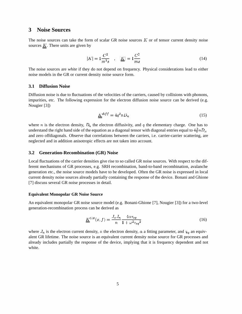
3 Noise Sources

The noise sources can take the form of scalar GR noise sources � or of tensor current density noisesources � . There units are given by

��

��, ��

��

�(14)

The noise sources are white if they do not depend on frequency. Physical considerations lead to eithernoise models in the GR or current density noise source form.

3.1 Diffusion Noise

Diffusion noise is due to fluctuations of the velocities of the carriers, caused by collisions with phonons,impurities, etc. The following expression for the electron diffusion noise source can be derived (e.g.Nougier [3])

�� (15)

where � is the electron density, �� the electron diffusivity, and � the elementary charge. One has tounderstand the right hand side of the equation as a diagonal tensor with diagonal entries equal to ��

and zero offdiagonals. Observe that correlations between the carriers, i.e. carrier-carrier scattering, areneglected and in addition anisotropic effects are not taken into account.

3.2 Generation-Recombination (GR) Noise

Local fluctuations of the carrier densities give rise to so called GR noise sources. With respect to the dif-ferent mechanisms of GR processes, e.g. SRH recombination, band-to-band recombination, avalanchegeneration etc., the noise source models have to be developed. Often the GR noise is expressed in localcurrent density noise sources already partially containing the response of the device. Bonani and Ghione[7] discuss several GR noise processes in detail.

Equivalent Monopolar GR Noise Source

An equivalent monopolar GR noise source model (e.g. Bonani-Ghione [7], Nougier [3]) for a two-levelgeneration-recombination process can be derived as

��

�!�� !��

(16)

where �� is the electron current density, � the electron density, � a fitting parameter, and !�� an equiv-alent GR lifetime. The noise source is an equivalent current density noise source for GR processes andalready includes partially the response of the device, implying that it is frequency dependent and notwhite.

5

Bulk Flicker GR-Noise

Taking a range of GR lifetimes into account a flicker GR noise model can be derived (van der Ziel [8],p. 125 ff)

��

��"� � �!�#!��

�$%&�$�� !�� $%&�$�� !�� (17)

where �� is a parameter, � �"� , and the time constants fulfill !� ' !�. With increasing frequencythe noise source changes from constant to �#� behavior close at the frequency �� #!�, and finally atfrequency �� #!� to a �#�� range.

4 Noise Figure

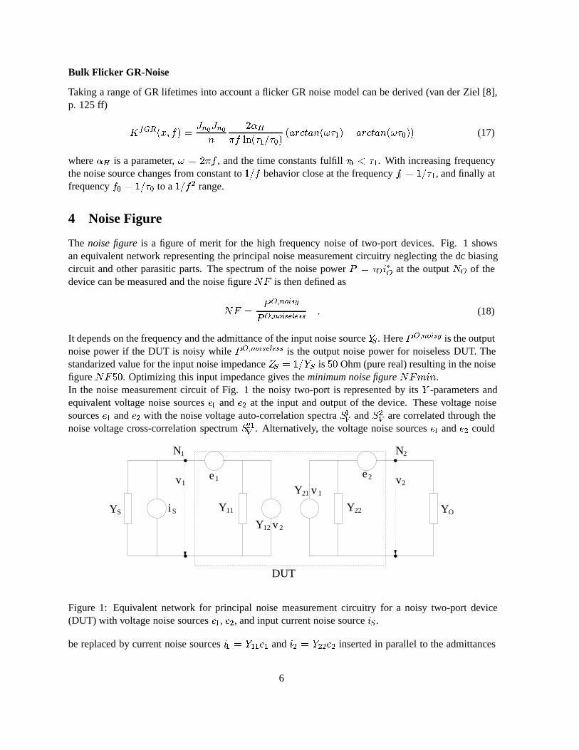
The noise figure is a figure of merit for the high frequency noise of two-port devices. Fig. 1 showsan equivalent network representing the principal noise measurement circuitry neglecting the dc biasingcircuit and other parasitic parts. The spectrum of the noise power ( � )�*

�

� at the output �� of thedevice can be measured and the noise figure �� is then defined as

�� (��

(��. (18)

It depends on the frequency and the admittance of the input noise source +� . Here (�� is the outputnoise power if the DUT is noisy while (�� is the output noise power for noiseless DUT. Thestandarized value for the input noise impedance �� #+� is �� Ohm (pure real) resulting in the noisefigure ��. Optimizing this input impedance gives the minimum noise figure �� *�.In the noise measurement circuit of Fig. 1 the noisy two-port is represented by its + -parameters andequivalent voltage noise sources ,� and ,� at the input and output of the device. These voltage noisesources ,� and ,� with the noise voltage auto-correlation spectra �� and �� are correlated through thenoise voltage cross-correlation spectrum �� . Alternatively, the voltage noise sources ,� and ,� could

Y11 Y22

N1 N2

e1 e2

21 1Y v

12 2Y v

1v 2v

iS

DUT

SY OY

Figure 1: Equivalent network for principal noise measurement circuitry for a noisy two-port device(DUT) with voltage noise sources ,�, ,�, and input current noise source *� .

be replaced by current noise sources *� � +��,� and *� � +��,� inserted in parallel to the admittances

6

+�� and +��, respectively. The auto-correlation spectra of these current noise sources are �� +��

and �� +�� , respectively, and their cross-correlation is given by �� +��+

�

�� .

The noisy input admittance +� has a current noise spectrum �� -�.�,�+�� and is thereforecomplemented by the input current noise source *� .The noise figure �� can be derived as

��

��

��

��+� � +��+��

�� ,

�+� � +��+��

��

�. (19)

The noise figure �� has exactly one mimimum for positive real part �,�+�� of the input admittance.Minimizing the noise figure �� wrt the input admittance +� gives the optimal input admittance +��

as

�,�+��

��

��,�+�� ,�� +

�

��

� �+��

��

��

��

(20)

/ �+�� / �+��

��/ �� +

�

�� . (21)

5 Numerical Approach

For the numerical computation of the device Green functions for each observation node an efficientalgorithm based on a block decomposition of the (Fourier transformed) Jacobian matrix is used. Thealgorithm is based on the approach of Bonani, Ghione, Pinto and Smith reported in [2] and extended tobe used in the mixed-mode framework of Dessis-�� thereby taking all the different contact boundaryconditions into account.We describe the algorithm for the situation of one noisy physical device furnished with a spatial dis-cretization grid of � internal vertices. The discretized (Fourier transformed) equation (3) has then theform �

� 0 �

��Æ�Æ1

��

��

�(22)

where the complex matrix � is the Jacobian of the internal device equations wrt the internal variables,0 the coupling of these equations to the circuit variables. � and are the Jacobians of the circuitresp. boundary condition equations wrt the circuit/boundary resp. the internal device variables. Therhs ��

��

� represents the discretized Æ-function at one vertex of the grid, and Æ��

Æ�Æ1

� is the

perturbated solution splitted into the internal part Æ� and the boundary and circuit part Æ1.To compute the potential Green functions wrt perturbations in one continuity equation for one obser-vation node we have to solve the given system for � different rhs corresponding to the discretizedÆ-functions in all grid vertices. This can be written in the matrix form�

� 0 �

��Æ2Æ+

��

�(�(�

�(23)

where ( ��

�(�(�

�has � columns, each representing a discretized Æ-function at one grid point. Using

a blocked decomposition method the numerical burden can be drastically reduced. Instead of solving

7

the complete linear system one reduces the system due to the fact that one is only interested in certainvalues of Æ1. The Schur decomposition of the matrix results in the equation�

� ��0� � � ��0

��Æ2Æ+

��

��(�

(� � ��(�

�(24)

or looking only onto the second component � � ��0

�Æ+ � (� � �

��(� (25)

With the substitution + �� we solve the equation

� + � (26)

followed by the solution of the reduced equation (25). The Green function for a circuit node * is thengiven by

��!� � Æ+ �! . (27)

Suitable choices of the perturbation matrix ( give the necessary potential Green function�� and �wrt both continuity equations for each observation node.The same procedure is performed in the case of mixed-mode simulations with several physical noisydevices. In this situation the matrix � is block diagonal, i.e.

� �

�� 3 3 3 �...

. . ....

� 3 3 3 ��

�� (28)

and the perturbation matrix ( is extended by discretizations of Æ-functions for all grid points of all noisydevices.The whole algorithm is interfaced to both the direct linear solvers Pardiso-�� and Super-�� and the it-erative solver Slip-�� of Dessis-�� . Besides the real extended formulation of the linear equations alsothe complex formulation can be assembled. This allows to put the complex mode of Pardiso-�� intoaction, which is most efficiently used in the case of up to several thousand vertices.

8

6 Noise Simulation with Dessis-��

6.1 General Remarks

The noise analysis capabilities in Dessis-�� can be used by selecting observation nodes (via the key-word ObservationNode within an ACCoupled solve-statement) and several noise source models in thephysics-sections of the physical devices (via the keyword Noise).

6.2 Noisy ACCoupled

The observation nodes are selected in an ACCoupled solve statement, where also the noise extractionfile and the fileprefix for noise plots are specified. A typical noisy ACCoupled looks like the followingexample:

ACCoupled (StartFrequency = 1.e8 EndFrequency 1.e11NumberOfPoints = 7 DecadeNode ( n_drain n_gate )Exclude ( v_drain v_gate )ObservationNode ( n_drain n_gate )ACExtraction = "mos"NoiseExtraction = "mos"NoisePlot = "mos") {poisson electron hole contact circuit

}

The keyword ObservationNode enables the noise analysis. Please observe that in the current implemen-tation the observation nodes have to be a subset of the nodes specified in Node ( ... ).The noise auto- and cross-correlation spectral densities for all observation nodes are plotted into the file

'noise-extraction4 noise des.plt .If not specified the default ”noiseextraction noise des.plt” is used.The 'noise-plot4 string serves as a prefix for device specific plots and refers to the NoisePlot sectionfor each device (see 6.5). For the auto-correlation noise data the filenames

'noise-plot4 'device-name4 'ob-node4 'number4 acgf des.datare created while for the cross-correlation noise data the filenames

'noise-plot4 'device-name4 'ob-node-14 'ob-node-24 'number4 acgf des.datare used, where 'ob-node4 is the observation node name, and the 'number4 is increased for eachcomputed frequency. The default is to write these files compressed (extension .Z). This can explicitly bespecified or switched off with the keyword [-] Compressed.The selection of the frequencies for which the noise analysis is performed is like in the ac analysis.With the Exclude statement the type of boundary conditions for non observation nodes can be modified.For the observation nodes the strong couplings to voltage sources is ”excluded” because otherwise theobserved noise voltage is zero.

9

6.3 Green Functions

The most cpu consuming part within the noise analysis is the computation of the complex (Fouriertransformed) Green functions. For the currently implemented noise source models only the PoissonGreen function wrt perturbations in both continuity equations at the specified observation nodes are of

interest, i.e.�� and

� .

The real and imaginary (Re/Im) part of the complex potential (Po) Green functions wrt perturbations in

the electron continuity (EC) equation�� can be plotted into the auto-correlation noise plot file as

PoECReACGreenFunction and PoECImACGreenFunctionfor all devices and given observation nodes. The terms

GradPoECReACGreenFunction and GradPoECImACGreenFunction

refer to the corresponding parts of the vector Green function�� , while

Grad2PoECACGreenFunction

refers to the absolute square of�� . Corresponding expressions are valid for perturbations in the hole

continuity (HC) equation.

6.4 Noise Sources

The noise sources of section 3 can be enabled for all physical devices in the physics section of theDessis-�� -command file

Physics {...Noise ( DiffusionNoise MonopolarGRNoise FlickerGRNoise )

}

and specified like the other physical parameters for regions resp. for materials. The standard inheritanceof physics parameters applies.

6.4.1 Diffusion Noise

The implemented diffusion noise source DiffusionNoise uses the Einstein relation � � 0 5 in equation(15) and results for electrons in the expression

�� -�.5� (29)

for the term on the diagonal, where � is the electron density, 5� the electron mobility, and T the latticeor electron temperature. The corresponding expression is used for holes. With the specification

DiffusionNoise ( <temp> )

where 'temp4 is one of LatticeTemperature, eTemperature, hTemperature, or e h Temperature, theused temperature in the expression can be chosen. Default is LatticeTemperature. For example eTem-perature uses the electron temperature for the the electron noise source while the lattice temperature isused for the hole noise source; the specification e h Temperature uses for the carrier noise source thecorresponding carrier temperature.

10

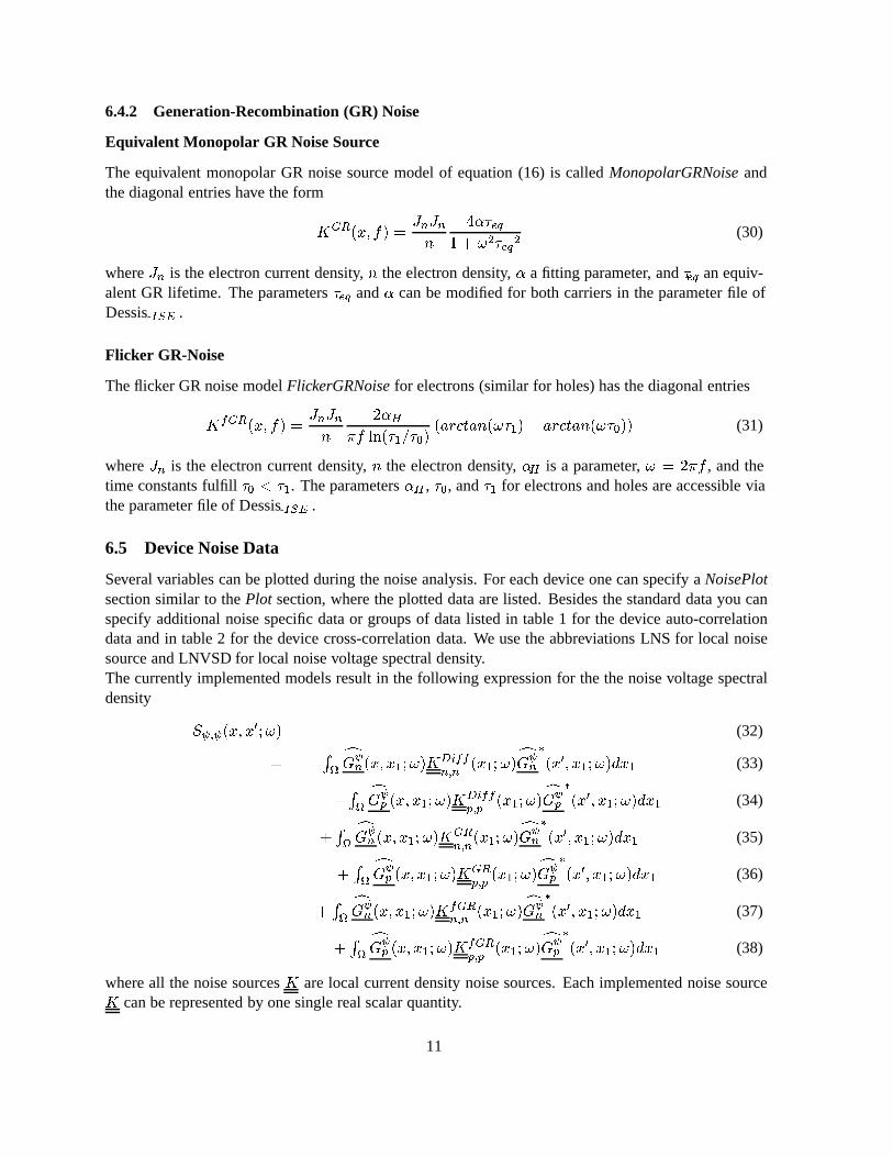
6.4.2 Generation-Recombination (GR) Noise

Equivalent Monopolar GR Noise Source

The equivalent monopolar GR noise source model of equation (16) is called MonopolarGRNoise andthe diagonal entries have the form

��

�!�� !��

(30)

where �� is the electron current density, � the electron density, � a fitting parameter, and !�� an equiv-alent GR lifetime. The parameters !�� and � can be modified for both carriers in the parameter file ofDessis-�� .

Flicker GR-Noise

The flicker GR noise model FlickerGRNoise for electrons (similar for holes) has the diagonal entries

��

��"� � �!�#!��

�$%&�$�� !�� $%&�$�� !�� (31)

where �� is the electron current density, � the electron density, �� is a parameter, � �"� , and thetime constants fulfill !� ' !�. The parameters �� , !�, and !� for electrons and holes are accessible viathe parameter file of Dessis-�� .

6.5 Device Noise Data

Several variables can be plotted during the noise analysis. For each device one can specify a NoisePlotsection similar to the Plot section, where the plotted data are listed. Besides the standard data you canspecify additional noise specific data or groups of data listed in table 1 for the device auto-correlationdata and in table 2 for the device cross-correlation data. We use the abbreviations LNS for local noisesource and LNVSD for local noise voltage spectral density.The currently implemented models result in the following expression for the the noise voltage spectraldensity

�� (32)

��

��

"��

��

�

�� (33)

��

� ��

"��

��

�

�� (34)

��

��

��

��

�

�� (35)

��

� ��

��

��

�

�� (36)

��

��

��

��

�

�� (37)

��

� ��

��

��

�

�� (38)

where all the noise sources � are local current density noise sources. Each implemented noise source� can be represented by one single real scalar quantity.

11

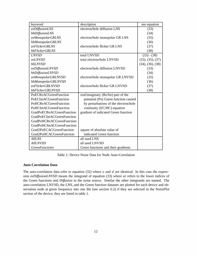
keyword description see equationeeDiffusionLNS electron/hole diffusion LNS (33)hhDiffusionLNS (34)eeMonopolarGRLNS electron/hole monopolar GR LNS (35)hhMonopolarGRLNS (36)eeFlickerGRLNS electron/hole flicker GR LNS (37)hhFlickerGRLNS (38)LNVSD total LNVSD (33) - (38)eeLNVSD total electron/hole LNVSD (33), (35), (37)hhLNVSD (34), (36), (38)eeDiffusionLNVSD electron/hole diffusion LNVSD (33)hhDiffusionLNVSD (34)eeMonopolarGRLNVSD electron/hole monopolar GR LNVSD (35)hhMonopolarGRLNVSD (36)eeFlickerGRLNVSD electron/hole flicker GR LNVSD (37)hhFlickerGRLNVSD (38)PoECReACGreenFunction real/imaginary (Re/Im) part of thePoECImACGreenFunction potential (Po) Green function causedPoHCReACGreenFunction by perturbations of the electron/holePoHCImACGreenFunction continuity (EC/HC) equationGradPoECReACGreenFunction gradient of indicated Green functionGradPoECImACGreenFunctionGradPoHCReACGreenFunctionGradPoHCImACGreenFunctionGrad2PoECACGreenFunction square of absolute value ofGrad2PoHCACGreenFunction indicated Green functionAllLNS all used LNSAllLNVSD all used LNVSDGreenFunctions Green functions and their gradients

Table 1: Device Noise Data for Node Auto-Correlation

Auto-Correlation Data

The auto-correlation data refer to equation (32) where � and �� are identical. In this case the expres-sion eeDiffusionLNVSD means the integrand of equation (33) where ee refers to the lower indices ofthe Green functions and Diffusion to the noise source. Similar the other integrands are named. Theauto-correlation LNVSD, the LNS, and the Green function datasets are plotted for each device and ob-servation node at given frequency into one file (see section 6.2) if they are selected in the NoisePlotsection of the device; they are listed in table 1.

12

keyword descriptionReLNVXVSD re/im part of total cross LNVSDImLNVXVSDReeeLNVXVSD re/im part of e/h cross LNVSDImeeLNVXVSDRehhLNVXVSDImhhLNVSDReeeDiffusionLNVXVSD re/im part ofImeeDiffusionLNVXVSD e/h diffusion cross LNVSDRehhDiffusionLNVXVSDImhhDiffusionLNVSDReeeMonopolarGRLNVXVSD re/im part ofImeeMonopolarGRLNVXVSD e/h monopolar GR cross LNVSDRehhMonopolarGRLNVXVSDImhhMonopolarGRLNVSDReeeFlickerGRLNVXVSD re/im part ofImeeFlickerGRLNVXVSD e/h flicker GR cross LNVSDRehhFlickerGRLNVXVSDImhhFlickerGRLNVSDAllLNVXVSD all used LNVXVSD

Table 2: Device Noise Data for Node Cross-Correlation

Cross-Correlation Data

In the case of � �� the node cross-correlation spectra are computed and the integrands becomecomplex. ReeeDiffusionLNVXVSD and ImeeDiffusionLNVXVSD refer to the real resp. imaginary partof the integrand of equation (33). A list of the node cross-correlation device data is given in table 2. Thecross-correlation LNVSD are plotted for each device and pair of observation nodes at given frequencyinto one file (see section 6.2) if they are selected in the NoisePlot section of the device; they are listedin table 2.

6.6 Node Noise Data

The noise analysis extracts for all given observation nodes the basic noise data and for all pairs ofobservation nodes the basic cross noise data. For each ACCoupled one file is generated accordingthe specification 'noise-extraction4 (see section 6.2). Table 3 lists all the data which are plotted foreach observation node, while table 4 lists all the possible cross noise data. The noise plot file can bepostprocessed to derive noise figures NF and NFmin (and additional features).

13

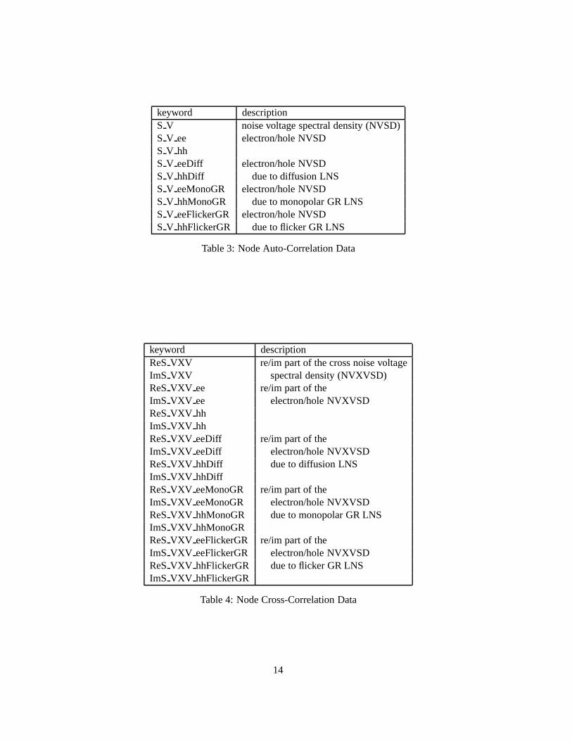
keyword descriptionS V noise voltage spectral density (NVSD)S V ee electron/hole NVSDS V hhS V eeDiff electron/hole NVSDS V hhDiff due to diffusion LNSS V eeMonoGR electron/hole NVSDS V hhMonoGR due to monopolar GR LNSS V eeFlickerGR electron/hole NVSDS V hhFlickerGR due to flicker GR LNS

Table 3: Node Auto-Correlation Data

keyword descriptionReS VXV re/im part of the cross noise voltageImS VXV spectral density (NVXVSD)ReS VXV ee re/im part of theImS VXV ee electron/hole NVXVSDReS VXV hhImS VXV hhReS VXV eeDiff re/im part of theImS VXV eeDiff electron/hole NVXVSDReS VXV hhDiff due to diffusion LNSImS VXV hhDiffReS VXV eeMonoGR re/im part of theImS VXV eeMonoGR electron/hole NVXVSDReS VXV hhMonoGR due to monopolar GR LNSImS VXV hhMonoGRReS VXV eeFlickerGR re/im part of theImS VXV eeFlickerGR electron/hole NVXVSDReS VXV hhFlickerGR due to flicker GR LNSImS VXV hhFlickerGR

Table 4: Node Cross-Correlation Data

14

6.7 Noise Figure

For two-port devices the noise figure �� can be extracted as well as minimized wrt to the input admit-tance, resulting in the mimimum noise figure �� *� and the optimized value +��.The extraction is based on a single device simulation to extract both the + -parameters of the two-portand the open-circuit equivalent noise voltage auto- and cross-correlation spectra for the input and outputnodes. An example simulation for a MOSFET is given in Appendix C. With the specified node list the+ -parameters are extracted under the condition of grounded source and substrate nodes, while for theinput (gate) and output (drain) the appropriate boundary conditions are imposed. The specification forthe observation nodes allows the computation of the auto- and cross-correlation spectra of the equivalentopen-circuit noise voltages at input and output node.The noise figure extraction script (see Appendix D) performs the computation of the auto- and cross-correlation noise current spectra �� , �� , and �� , the noise figure �� , the optimized input admittance+��, and the minimum noise figure �� *�. The user has to adjust the extraction script to the actualsimulation:

names of the actual ac and noise simulation files

names of the input and output nodes

selection of the displayed curves.

With the command

inspect -f nf_ins.cmd

Inspect-�� is invoked and displays the selected curves. Observe that the sequence of the creation ofcurves should not be changed because the computation of the curves (partially) depends on the existenceof preceding ones.

15

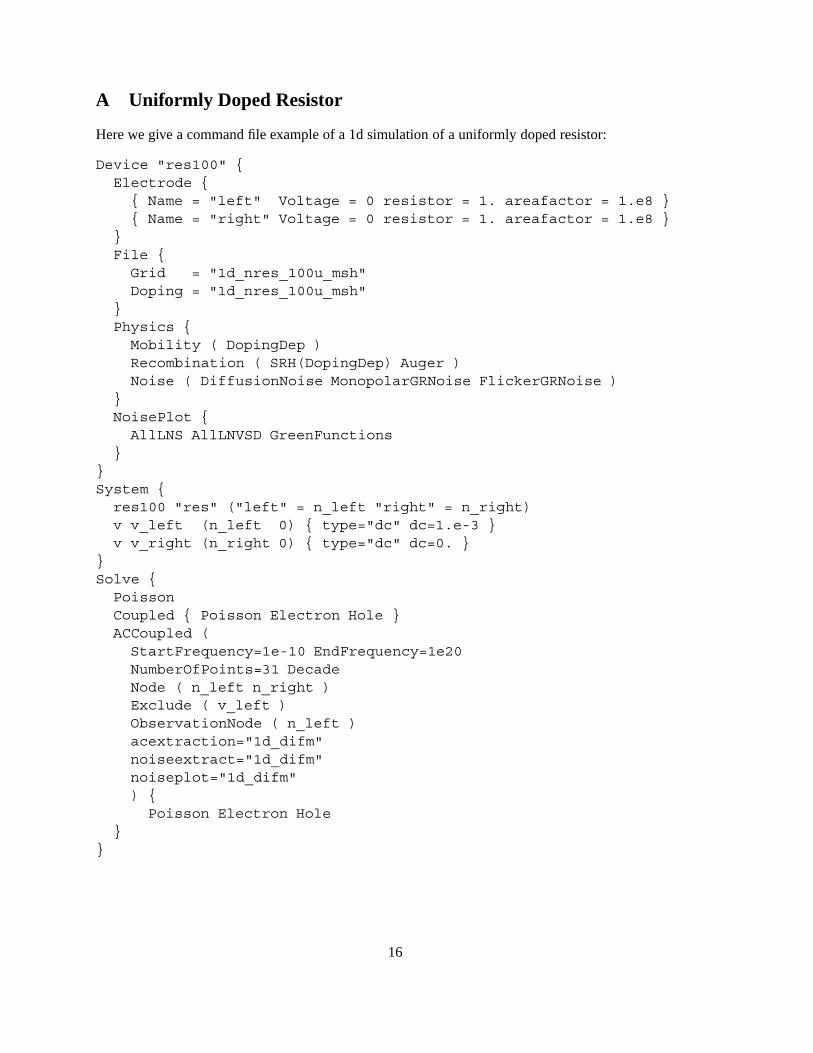
A Uniformly Doped Resistor

Here we give a command file example of a 1d simulation of a uniformly doped resistor:

Device "res100" {Electrode {{ Name = "left" Voltage = 0 resistor = 1. areafactor = 1.e8 }{ Name = "right" Voltage = 0 resistor = 1. areafactor = 1.e8 }

}File {Grid = "1d_nres_100u_msh"Doping = "1d_nres_100u_msh"

}Physics {Mobility ( DopingDep )Recombination ( SRH(DopingDep) Auger )Noise ( DiffusionNoise MonopolarGRNoise FlickerGRNoise )

}NoisePlot {AllLNS AllLNVSD GreenFunctions

}}System {res100 "res" ("left" = n_left "right" = n_right)v v_left (n_left 0) { type="dc" dc=1.e-3 }v v_right (n_right 0) { type="dc" dc=0. }

}Solve {PoissonCoupled { Poisson Electron Hole }ACCoupled (StartFrequency=1e-10 EndFrequency=1e20NumberOfPoints=31 DecadeNode ( n_left n_right )Exclude ( v_left )ObservationNode ( n_left )acextraction="1d_difm"noiseextract="1d_difm"noiseplot="1d_difm") {Poisson Electron Hole

}}

16

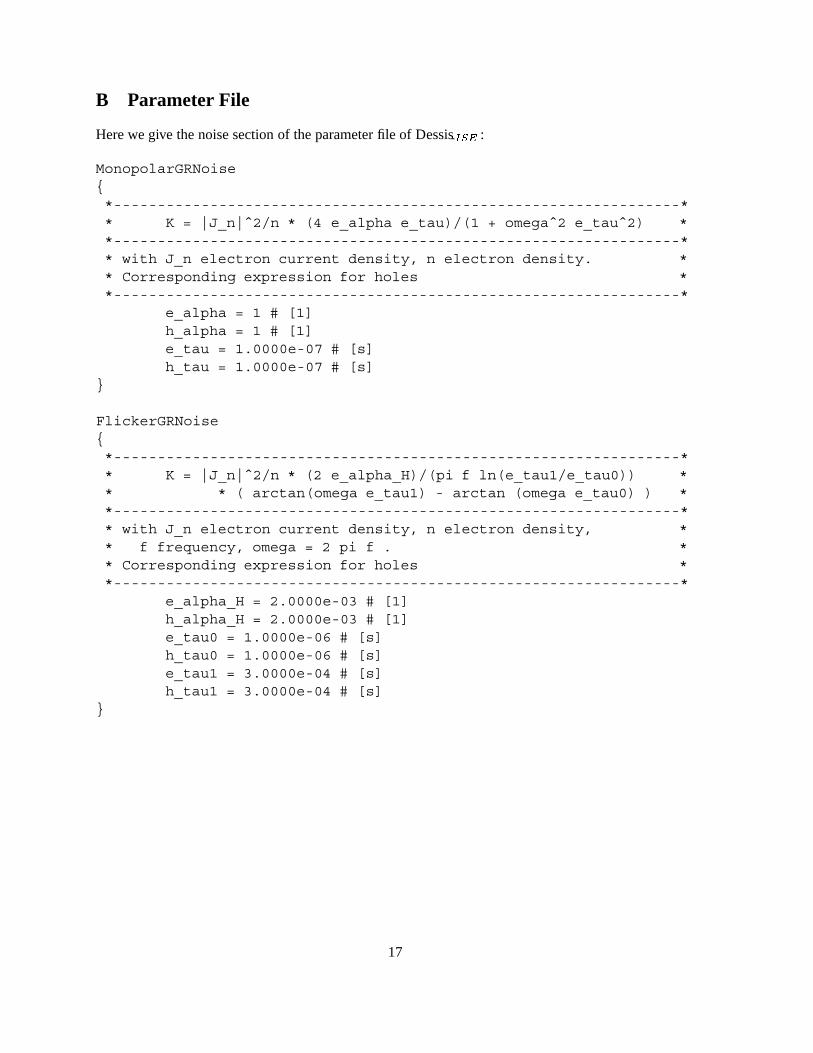
B Parameter File

Here we give the noise section of the parameter file of Dessis-�� :

MonopolarGRNoise{*-----------------------------------------------------------------** K = |J_n|ˆ2/n * (4 e_alpha e_tau)/(1 + omegaˆ2 e_tauˆ2) **-----------------------------------------------------------------** with J_n electron current density, n electron density. ** Corresponding expression for holes **-----------------------------------------------------------------*

e_alpha = 1 # [1]h_alpha = 1 # [1]e_tau = 1.0000e-07 # [s]h_tau = 1.0000e-07 # [s]

}

FlickerGRNoise{*-----------------------------------------------------------------** K = |J_n|ˆ2/n * (2 e_alpha_H)/(pi f ln(e_tau1/e_tau0)) ** * ( arctan(omega e_tau1) - arctan (omega e_tau0) ) **-----------------------------------------------------------------** with J_n electron current density, n electron density, ** f frequency, omega = 2 pi f . ** Corresponding expression for holes **-----------------------------------------------------------------*

e_alpha_H = 2.0000e-03 # [1]h_alpha_H = 2.0000e-03 # [1]e_tau0 = 1.0000e-06 # [s]h_tau0 = 1.0000e-06 # [s]e_tau1 = 3.0000e-04 # [s]h_tau1 = 3.0000e-04 # [s]

}

17

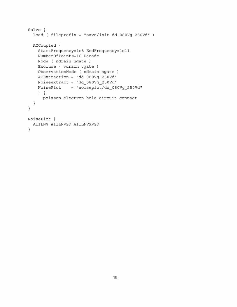
C NF Simulation of a MOSFET

Here we give an example for a HF simulation of a MOSFET suitable for a noise figure extraction:

Device "nmos" {Electrode {{ name=source voltage=0. resistance=1. AreaFactor=200 }{ name=gate voltage=0. resistance=1. AreaFactor=200

barrier=-0.45}{ name=drain voltage=0. resistance=1. AreaFactor=200 }{ name=bulk voltage=0. resistance=1. AreaFactor=200 }

}Physics {Recombination ( SRH(DopingDep) Auger Avalanche(Lackner) )Mobility ( DopingDep Enormal HighFieldSaturation )Noise ( DiffusionNoise )

}InterfaceConditions {{ region = (0,1) RecombVelocity = 500 Charge = 4e10 }

}File {Grid = "n21_mdr.grd"Doping = "n21_mdr.dat"param = "nmos.par"

}}

Math {Method = BlockedSubmethod = PardisoDerivativesAvalDerivativesNewDiscretization

}

System {nmos "NMOS" ( "source" = nsource "gate" = ngate

"drain" = ndrain "bulk" = nbulk )

v vgate ( ngate 0 ) { type="dc" dc=0. }v vsource ( nsource 0 ) { type="dc" dc=0. }v vbulk ( nbulk 0 ) { type="dc" dc=0. }v vdrain ( ndrain 0 ) { type="dc" dc=0. }

}

18

Solve {load ( fileprefix = "save/init_dd_080Vg_250Vd" )

ACCoupled (StartFrequency=1e8 EndFrequency=1e11NumberOfPoints=16 DecadeNode ( ndrain ngate )Exclude ( vdrain vgate )ObservationNode ( ndrain ngate )ACExtraction = "dd_080Vg_250Vd"Noiseextract = "dd_080Vg_250Vd"NoisePlot = "noiseplot/dd_080Vg_250Vd") {poisson electron hole circuit contact

}}

NoisePlot {AllLNS AllLNVSD AllLNVXVSD

}

19

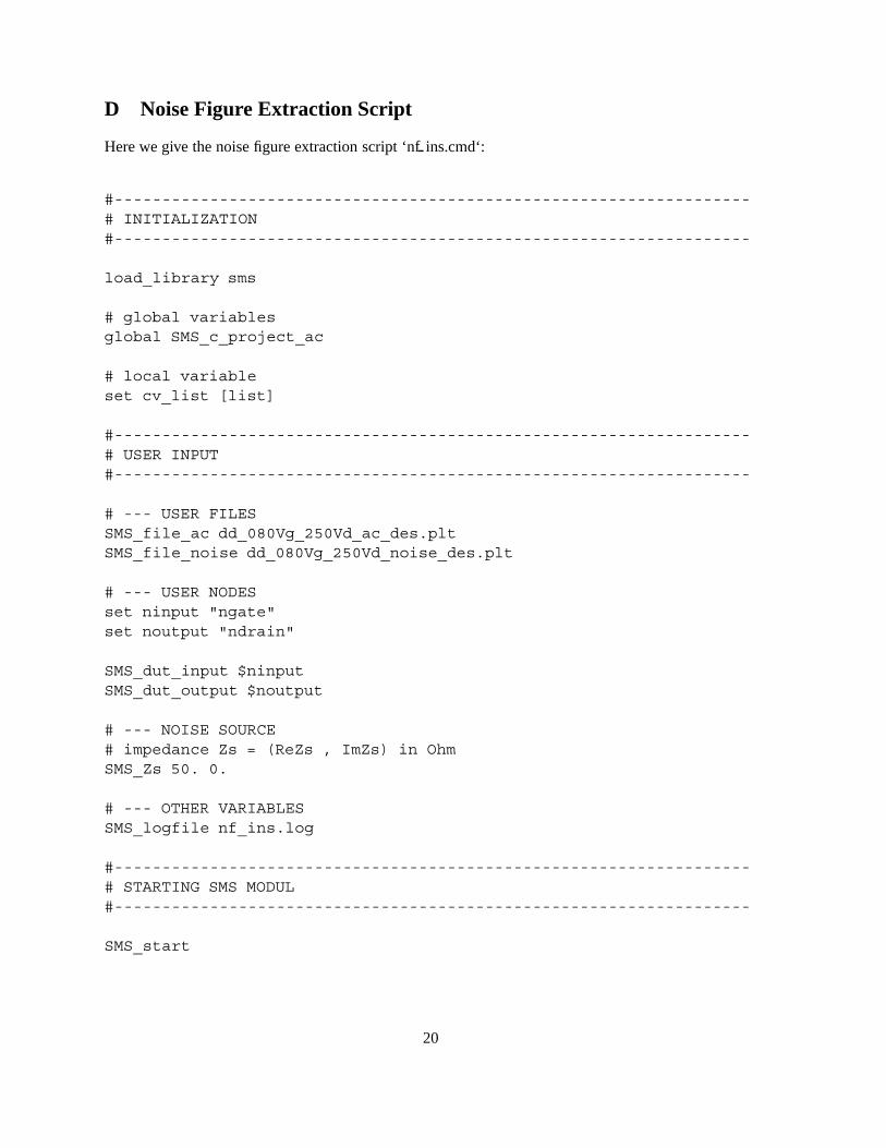
D Noise Figure Extraction Script

Here we give the noise figure extraction script ‘nf ins.cmd‘:

#-------------------------------------------------------------------# INITIALIZATION#-------------------------------------------------------------------

load_library sms

# global variablesglobal SMS_c_project_ac

# local variableset cv_list [list]

#-------------------------------------------------------------------# USER INPUT#-------------------------------------------------------------------

# --- USER FILESSMS_file_ac dd_080Vg_250Vd_ac_des.pltSMS_file_noise dd_080Vg_250Vd_noise_des.plt

# --- USER NODESset ninput "ngate"set noutput "ndrain"

SMS_dut_input $ninputSMS_dut_output $noutput

# --- NOISE SOURCE# impedance Zs = (ReZs , ImZs) in OhmSMS_Zs 50. 0.

# --- OTHER VARIABLESSMS_logfile nf_ins.log

#-------------------------------------------------------------------# STARTING SMS MODUL#-------------------------------------------------------------------

SMS_start

20

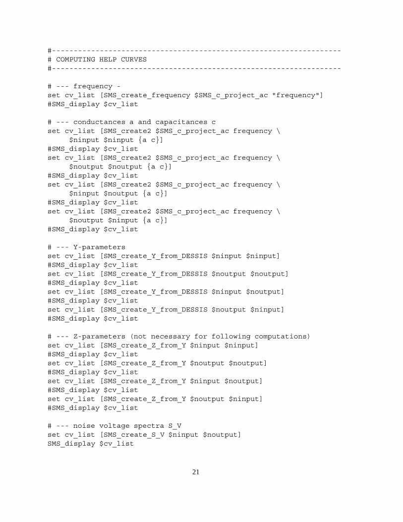
#-------------------------------------------------------------------# COMPUTING HELP CURVES#-------------------------------------------------------------------

# --- frequency -set cv_list [SMS_create_frequency $SMS_c_project_ac "frequency"]#SMS_display $cv_list

# --- conductances a and capacitances cset cv_list [SMS_create2 $SMS_c_project_ac frequency \

$ninput $ninput {a c}]#SMS_display $cv_listset cv_list [SMS_create2 $SMS_c_project_ac frequency \

$noutput $noutput {a c}]#SMS_display $cv_listset cv_list [SMS_create2 $SMS_c_project_ac frequency \

$ninput $noutput {a c}]#SMS_display $cv_listset cv_list [SMS_create2 $SMS_c_project_ac frequency \

$noutput $ninput {a c}]#SMS_display $cv_list

# --- Y-parametersset cv_list [SMS_create_Y_from_DESSIS $ninput $ninput]#SMS_display $cv_listset cv_list [SMS_create_Y_from_DESSIS $noutput $noutput]#SMS_display $cv_listset cv_list [SMS_create_Y_from_DESSIS $ninput $noutput]#SMS_display $cv_listset cv_list [SMS_create_Y_from_DESSIS $noutput $ninput]#SMS_display $cv_list

# --- Z-parameters (not necessary for following computations)set cv_list [SMS_create_Z_from_Y $ninput $ninput]#SMS_display $cv_listset cv_list [SMS_create_Z_from_Y $noutput $noutput]#SMS_display $cv_listset cv_list [SMS_create_Z_from_Y $ninput $noutput]#SMS_display $cv_listset cv_list [SMS_create_Z_from_Y $noutput $ninput]#SMS_display $cv_list

# --- noise voltage spectra S_Vset cv_list [SMS_create_S_V $ninput $noutput]SMS_display $cv_list

21

# --- noise current spectra S_Iset cv_list [SMS_create_S_I $ninput $noutput]SMS_display $cv_list

#-------------------------------------------------------------------# NOISE FIGURES NF and NFmin and OPTIMIZED INPUT ADMITTANCE Ymin#-------------------------------------------------------------------# you can choose one (or more) of following branches# (A) NF computation# (B) NFmin computation#-------------------------------------------------------------------

# --- (A) NF computation -set cv_list [SMS_create_NF $ninput $noutput]SMS_display $cv_list

set cv_list [SMS_create_NF_db20 $ninput $noutput]#SMS_display $cv_list

#-------------------------------------------------------------------

# --- (B) NFmin computation -set cv_list [SMS_create_Ymin $ninput $noutput]#SMS_display $cv_list

set cv_list [SMS_create_NFmin $ninput $noutput]SMS_display $cv_list

set cv_list [SMS_create_NFmin_db20 $ninput $noutput]#SMS_display $cv_list

#-------------------------------------------------------------------# END OF SMS MODUL#-------------------------------------------------------------------

22

References

[1] W. Shockley, J. A. Copeland, and R. P. James, “The impedance field method of noise calculation inactive semiconductor devices,” in Quantum Theory of Atoms, Molecules and the Solid State (P.-O.Loewdin, ed.), pp. 537–563, Academic Press, 1966.

[2] F. Bonani, G. Ghione, M. R. Pinto, and R. K. Smith, “An efficient approach to noise analysis throughmultidimensional physics-based models,” IEEE Trans. Electron Devices, vol. 45, pp. 261–269, Jan.1998.

[3] J.-P. Nougier, “Fluctuations and noise of hot carriers in semiconductor materials and devices,”IEEE Trans. Electron Devices, vol. 41, pp. 2034–2049, Nov. 1994.

[4] A. Kunzmann, “Simulation of noise in semiconductor devices,” Tech. Rep. 98/7, Integrated SystemsLaboratory, Swiss Federal Institute of Technology Zurich, Switzerland, 1998.

[5] T. C. McGill, M.-A. Nicolet, and K. K. Thornber, “Equivalence of the Langevin method and theimpedance-field method of calculating noise in devices,” Solid-State Eletronics, vol. 17, pp. 107–108, 1974.

[6] C. M. van Vliet, “Macroscopic and microscopic methods for noise in devices,” IEEE Trans. Elec-tron Devices, vol. 41, pp. 1902–1915, Nov. 1994.

[7] F. Bonani and G. Ghione, “Generation-recombination noise modelling in semiconductor devicesthrough population or approximate equivalent current density fluctuations,” Solid-State Eletronics,vol. 43, pp. 285–295, 1999.

[8] A. van der Ziel, Noise in Solid State Devices and Circuits. A Wiley-Interscience Publication, JohnWiley & Sons, Inc., 1986.

23

Simulation of Noise in Semiconductor Devices with Dessis ...schenk/noiseTechRep2.pdf · modern...

Documents

Transcript of Simulation of Noise in Semiconductor Devices with Dessis ...schenk/noiseTechRep2.pdf · modern...