Simulation of Lumbar Spine Biomechanics Using Abaqus€¦ · Simulation of Lumbar Spine...

Simulation of Lumbar Spine Biomechanics Using Abaqus

Dana Coombs*, Milind Rao†, Michael Bushelow*, James Deacy†, Peter Laz, and Paul Rullkoetter†

*Synthes Spine, West Chester, PA †University of Denver, Denver, CO

Abstract: Biomechanics testing of the lumbar spine, using cadaveric specimens, has the advantage of using actual tissue, but has several disadvantages including variability between specimens and difficultly acquiring measures such as disc pressure, bone strain, and facet joint contact pressure. A simulation model addresses all of these disadvantages. The objective of this work is to develop a method to simulate the biomechanics of the lumbar spine.

A process is currently being used to convert a CT scan of a lumbar spine into a simulation model. The process includes converting the CT scan to a geometry file, creating a mesh of the bone and soft tissue, and assigning material properties to each element of the bone based on the bone density. Finally, the model is solved using Abaqus Explicit. Optimization techniques are used to tune uncertain material properties to match the kinematics of the simulation model to actual cadaveric test results.

In addition, techniques have been explored to greatly reduce the computational time for the model. The soft tissue, discs, and ligaments were replaced with simplified mechanical constrains (ball-in-socket joints and non-linear, 3 dimensional torsional springs) and the vertebrae are rigid. This technique can be used for all or a portion of the spine.Further efforts are being pursued to simplify the workflow from CT scan to simulation model.

This model can be used to simulate the performance of implants including total disc replacement and fusion techniques such as interbody spacers with rods and pedicle screws.

Keywords: Spine, Biomechanics, Explicit, Kinematics, Disc, Vertebrae, Vertebral Body, Lumbar, CT Scan, Experimental Validation, Motion Tracking

1. Introduction

Biomechanics testing of the spine is currently used to evaluate the performance of spine implants such as total disc replacements and fusion systems. This is typically done by applying loads such as compression and moments to multi-segmental spine or a functional spinal unit (FSU). The intact condition is tested first, and then the spine is instrumented with implants and tested again. Kinematic measures such at rotation and translation are measured for each level of the spine using a motion tracking system. Axial, shear and moment loads are measured with a six degree of freedom load cell. Other metrics can be calculated from these measures such as the instant center

2011 SIMULIA Customer Conference 1

Visit the SIMULIA Resource Center for more customer examples.


http://www.3ds.com/products/simulia/resource-center/by-industry/


of rotation between two vertebrae. These measures are used to compare implants to each other and to the intact spine.

Biomechanics testing of the spine using cadaver tissue has several challenges and disadvantages. The first challenge relates to acquiring and selecting the cadaveric specimens to plan a relevant test. Criterion for selection often includes the quality of bone and amount of osteoporosis, the amount and grade of disc degeneration, disc height, and overall specimen size. Even with careful specimen selection, there is always significant variability between specimens, which makes comparisons less reliable. Also, some measures, in addition to the ones mentioned above, are difficult or impossible to acquire. These include bone strain, disc pressure, and facet contact pressure or reaction load. Finally, biomechanics testing is very time consuming and expensive.

Based on these challenges, a simulation model of the spine becomes a very attractive alternative. Several validated simulation models for varying disease states can be useful to design implants virtually. A simulation model can be used to evaluate and drive the design of implants before they are fully detailed and prototyped. All of the challenging measures mentioned above can be extracted from the model and all the variability in real tissue is removed. However, a simulation model must be properly validated based on actual biomechanics data.

2. Materials and Methods

A CT scan of a healthy 48 year old female lumbar spine, as shown in Figure 1, was used to develop the IGES geometry for the model. ScanIP (Simpleware, Exeter, UK) was used to do this conversion. The geometry was then imported into HyperMesh (Altair, Troy, MI). For the situations when the spine was instrumented with an implant, the CAD file was also imported into HyperMesh. BoneMat was used to determine the Young’s modulus for each element in the mesh. This is done by correlating the Hounsfield unit from the CT scan to Young’s modulus of the bone (Morgan, 2003). Figure 2 shows the material property variation for each element in the mesh. The disc was defined with annular rings to represent the annulus fibrosis, which were divided into four quadrants and meshed with 8-noded hexahedral elements and embedded crisscross fibers represented as spring elements. The nucleus pulposus was modeled as a fluid filled cavity. Figure 2 shows the model of the disc. All the major ligaments of the spine were modeled as two-noded 3D connector elements (CONN3D2). These include the Anterior Longitudinal Ligament (ALL), the Posterior Longitudinal Ligament (PLL), The Superspinous Ligament (SSL), the Intraspinous ligament (ISL), the Intratransverse Ligament (ITL), Ligamentum Flavum (LF), and the Facet Capsular Ligament (FCL). Reference nodes were placed at the center of the vertebral bodies at each end of the spine (L1 and L5) for the purposes of applying boundary conditions. The nodes at the end plates of the L1 and L5 vertebrae were tied to corresponding reference node with beam elements. Figure 3 shows the model in Abaqus CAE. The inferior vertebra, L5, was constrained in all degrees of freedom at the reference node. The superior vertebra, L1, was loaded with pure moments to cause flexion and extension. Other moments could be applied to cause lateral bending and axial rotation. All cartilage was rigid and meshed with 8-noded hexahedral elements. Contact was defined with a pressure-overclosure relationship based on prior computational efficiency studies. “(Rao, 2009).” Finally, the input files were created and the model was solved using Abaqus/Explicit (Simulia, Providence, RI). Figure 4 shows the work flow.

2 2011 SIMULIA Customer Conference

Figure 1. CT scan of lumbar spine.


Figure 2. Variation of element properties and model of disc.


Figure 3. Full lumbar model in Abaqus CAE.


CT scan

Scan IPInput: dicomOutput: STL

HypermeshInput: STLOutput: inp

Abaqus Solver

C

Input: STLOutput: odb

Abaqus CAE/PostInput: odb

Output: txt, bmp, xls, avi

AD ImplantInput: igs

BoneMatInput: cct, inp

Python Custom ScriptsInput: odb

Output: txt, xls

Figure 4. Scan to model workflow.

A manual optimization was performed on the flexion/extension torque-rotation behavior of the FSU and the entire lumbar spine by varying the mechanical properties of the soft tissues, while staying within the range of values reported in the literature for the structures. A summary of the properties used for the vertebrae, ligaments, annulus fibrosis, and nucleus pulposis are summarized in table 1.

Table 1. Properties of structures.

Structure Properties Reference Vertebral Bodies L4-L5 Material Mapped “(Morgan, 2003)” Ground Matrix (Annulus Fibrosis)

Hyperelastic (Neo-Hookean) with constants c1=0.25, c2=0.3

“(Eberlein, 2000)”

Nucleus Pulposis Fluid density=1370 kg/m3 Fluid bulk modulus=2.2E3 MPa

“(Eberlein, 2000)”

Intervertebral disc fibers Force-deflection curve “(Sharma, 1995)” Ligaments Force-deflection curve “(Chazal, 1985)” Facet cartilage Optimized pressure-overclosure relationship for rigid “(Mesfar, 2005)”

Two types of load cases were used. Pure flexion/extension, lateral bending, and axial rotation moments were applied to the spine. The second case was a combination of the pure moments with a “follower load”. A “follower load” is a compression load along the curvature of the lumbar spine (Patwardhan, 1999).

Another approach was used to greatly increase the efficiency of the solver run times. An analogue spine was used “(Laz, 2010)”, which represented the soft tissue as ball-in-socket joints and 3 rotational degree of freedom, non-linear springs. The center of the ball-in-socket was located at the average center of rotation from the fully deformable model. Figure 5 shows the computationally efficient model with emphasis on the disc. In addition, the vertebrae were modeled as rigid bodies. This approach could be used for most of the spine and detailed modeling could be used at the levels of interest. For this study, the disc and ligaments between L4 and L5


were fully modeled and the L4 and L5 vertebra were flexible while the rest of the spine was rigid with ball-in-socket joints.

Figure 5. Image of computationally efficient spine (zoom in on disc).

3. Results

Validations were performed on the whole spine under a variety of loading conditions. The endpoint of the loading cycle was used for comparisons with reported ranges of motion. Root mean square errors and the maximum absolute errors were computed between model predictions and available literature (experimental or model) data. Table 2 summarizes the comparison. In addition, the entire torque-rotation curve was compared (when available) in the current study in order to also consider potential non-linearity in behavior.


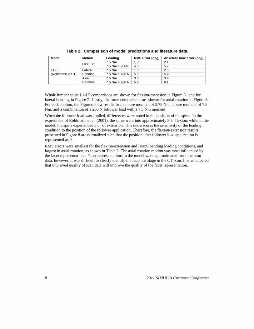
Table 2. Comparison of model predictions and literature data.

Model Motion Loading RMS Error (deg) Absolute max error (deg) 7.5 Nm 1.3 2.1

Flex-Ext 7.5 Nm + 280N 4.3 5.7 7.5 Nm 1.0 2.5 Lateral

Bending 7.5 Nm + 280 N 5.5 5.9 L1-L5

7.5 Nm 3.0 3.9 (Rohlmann 2001)

Axial Rotation 7.5 Nm + 280 N 5.6 6.1

Whole lumbar spine L1-L5 comparisons are shown for flexion-extension in Figure 6. and for lateral bending in Figure 7. Lastly, the same comparisons are shown for axial rotation in Figure 8. For each motion, the Figures show results from a pure moment of 3.75 Nm, a pure moment of 7.5 Nm, and a combination of a 280 N follower load with a 7.5 Nm moment.

When the follower load was applied, differences were noted in the position of the spine. In the experiment of Rohlmann et al. (2001), the spine went into approximately 5.5° flexion, while in the model, the spine experienced 3.0° of extension. This underscores the sensitivity of the loading condition to the position of the follower application. Therefore, the flexion-extension results presented in Figure 8 are normalized such that the position after follower load application is represented as 0.

RMS errors were smallest for the flexion-extension and lateral bending loading conditions, and largest in axial rotation, as shown in Table 2. The axial rotation motion was most influenced by the facet representations. Facet representations in the model were approximated from the scan data; however, it was difficult to clearly identify the facet cartilage in the CT scan. It is anticipated that improved quality of scan data will improve the quality of the facet representation.


Figure 6. Comparison of intact results for flexion/extension between L1-L5.


Figure 7. Comparison of intact results for lateral bending between L1-L5.


Based on flexion and extension with pure moments of 8Nm, the instant center of rotation (ICR) was determined based on the full range of motion and used to determine the “ball-in-socket” location for the surrogate model. Figure 8 shows the location of the ICR for each level of the lumbar spine. The surrogate model with a deformable L4-L5 disc compared well to the fully deformable model. The vertebral body rotations were within 0.11°, as shown in Figure 9. The disc pressure at L4-L5 were within 0.024 MPa and the annulus strain pattern was similar, as shown in Figure 10. The facet contact forces were within 3.4%, as shows in Figure 11, and the ligament recruitment pattern was similar. Finally, the computation time for the surrogate model with a deformable L4-L5 disc was less than 15% of the fully deformable model. When the surrogate model had a ball-in-socket joint for L4-L5, the computation time was less than 1% “(Laz 2010)”.

Figure 8. Location of ICR, • = instant center


Figure 9. Comparison of surrogate to fully deformable model – vertebral body rotation.

-8

-4

0

4

8

-4 -2 0 2 4 6 8

Figure 10. Comparison of surrogate to fully deformable model – disc pressure and annulus strain.

Fully deformable

Flex. -Ext.

Lat. Bend.

Axial Rot.

Rotation [Deg]

-6

Torque [Nm]

Combined


Flex. Ext. Lat.Bend.

AxialRot.

Pre

ssu

re [

MP

a]0.3

0.2

0.1

00

25

50

75

100

125

Flexion Extension Lateral bend Axial rotation

Fac

et c

onta

ct f

orce

[N

]

L4-L5125

100

75

50

25

0Flex. Ext. Lat.

Bend.Axial

Fully deformable

Combined

L4-L5

Fl i E i L lB di A i l R i

Rot.

Figure 11. Comparison of surrogate to fully deformable model – Disc Pressure and facet contact forces.

4. Discussion

In general, FE model predictions agreed well with available data from the literature. Experimental data contained significant levels of variability due to inter-subject differences (e.g. Bowden et al., 2008). Comparisons were made for the whole lumbar L1-L5 under a variety of loading conditions depending on the available literature data.

The differences in accuracy between the various literature comparisons highlight the challenge of trying to tune a single specimen model to literature results for a variety of specimens. By tuning a specimen-specific model to experimental data collected on that specimen, the effects of inter-specimen variability can be greatly reduced and the fidelity of the model can be improved.

The surrogate model with a deformable disc, at the level of interest, proves to be a functionally equivalent model. The savings in computation time allows the model to be used for early design phase simulation of spine implant performance. The model can also be used for probabilistic and sensitivity studies related to implant position and implant size.

5. Conclusion

A simulation model eliminates the variability, cost and biohazards of cadaveric tissue. It is also able to provide data on measures that are difficult or impossible to acquire in a cadaveric tissue, such as disc pressure or bone strain. The simulation model can vary from fully deformable to computationally efficient, fully rigid with simplified ball-in-socket joints. These models must be validated according to actual biomechanics data to have confidence in predictability.

A simulation model of the lumbar spine is a powerful tool to predict biomechanics performance, and to design orthopedic implants. This can be done without using costly and time consuming cadaveric biomechanics tests. Some examples include total disc replacements, interbody fusion devices, pedicle screw and rod systems, and interspinous spacers.


6. References

1. Bowden, A.E., Guerin, H., Villarraga, M.L., Patwardhan, A.G., Ochoa, J.A., “Quality of motion considerations in numerical analysis of motion restoring implants of the spine,” Clinical Biomechanics 23: 536-44, 2008.

2. Chazal, J., Tanguy, A., Bourges, M., Gaurel, G., Escande, G., “Biomechanical properties of spinal ligaments and a histological study of the supraspinal ligament in traction,” Journal of Biomechanics 18: 167-76, 1985.

3. Eberlein, R., Holzapfel, G.A., Schulze-Bauer, C.A.J., “An anisotropic model for annulus tissue and enhanced finite element analyses of intact lumbar disc bodies,” Computer Methods in Biomechanics and Biomedical Engineering 4: 209-29, 2000.

4. Laz, P. J., Deacy, J., Patrella, A. J., Rao. M., “Combined rigid deformable surrogate model for computationally-efficient evaluation of spine mechanics,” ORS 2010.

5. Mesfar, W., Shirazi-Adl, A.,”Biomechanics of the knee joint in flexion under various quadriceps forces,” Knee 12, 424-434, 2005.

6. Morgan, E.F., Bayraktar, H.H., Keaveny, T.M., “Trabecular bone modulus-density relationships depend on anatomic site,” Journal of Biomechanics 36: 897–904, 2003.

7. Patwardhan A. G., Havey R. M., Meade K. P., Lee B., and Dunlap B., “A Follower Load Increases the Load-Carrying Capacity of the Lumbar Spine in Compression”, Spine, vol. 24, pp. 1003–1009, 1999.

8. Sharma, M., Langrana, N., Rodriguez, J., “Role of ligaments and facets in lumbar spinal stability,” Spine 20: 887-900, 1995.

9. Rao, M., Petrella, A.J., Baldwin, M.A., Laz, P.J., Rullkoetter, P.J., “Efficient probabilistic finite element modeling for evaluation of spinal mechanics.” Transactions of the ORS 34: 1771, 2009.




Simulation of Lumbar Spine Biomechanics Using Abaqus€¦ · Simulation of Lumbar Spine...

Documents

Transcript of Simulation of Lumbar Spine Biomechanics Using Abaqus€¦ · Simulation of Lumbar Spine...