Transportation Research Record 806

2 .

3.

4 .

5.

6 .

7 .

8 .

9.

Vehicle Weights and Dimensions. 141, 1973.

NCHRP, Rept.

Transportation and Development Around the Pa­cific. ASCE, New York, 1980. A Policy on Geometric Design of Rural High­ways. AASHO, Washington, DC, 1966. AASHTO. A Policy on Geometric Design of High­ways and Streets. NCHRP, Project 20-7, Task 14, Review Draft 2, Dec. 1979. D.E. Peterson and R. Gull. Triple Trailer Evaluation in Utah. Utah Department of Trans­portation, Salt Lake City, Final Rept., 1975. Report on the Testing of Triple Trailer Combi­nations in Alberta. Alberta Department of Highways and Transport, Edmonton, Alberta, Canada, 1970. Triple Trailer Study in California. California Division of Highways, Sacramento, 1972. Theoretical Evaluation of the Relative Braking Performance, Stability, and Hitch Point Forces of Articulated Vehicles. Research Institute, Illinois Institute of Technology, Chicago, 1976. Operations and Procedures Manual. Texas State Department of Highways and Public Transporta­tion, Austin, 1976.

21

10. Manual on Uniform Traffic Control Devices. AASHO, Washington, DC, 1970.

11. Offtracking Characteristics of Trucks and Truck Combinations. Western Highway Institute, San Francisco, Research Committee Rept. 3, 1970.

12. Horsepower Considerations for Trucks and Truck Combinations. Western Highway Institute, San Francisco, 1978.

13. A. Taragin. Effect of Roadway Width on Vehicle Operation. Public Roads, Vol. 24, No. 6, 1945.

14. State Law and Regulations on Truck Size, Weight, and Speed. R.J. Hansen Associates, Inc., Rockville, MD, 1978.

15. Roy Jorgensen Associates, Inc. Cost and Safety Effectiveness of Highway Design Elements. NCHRP, Rept. 197, 1978.

16. Federal Highway Administration. Highway Per-formance Monitoring System: Field Implementa­tion Manual. u.s. Government Printing Office, 1979.

Publication of this paper sponsored by Committee on Geometric Design.

Simulation of H ighway Traffic on Two-Lane, Two-Way

Rural Highways SHIE-SHIN WU AND CLINTON L. HEIMBACH

A summary is presented of research undertaken to develop a rural two-lane, two-way computer simulation model that could be used by the highway design practitioner to measure and evaluate traffic-flow consequences for various alternatives considered during the roadway design process. To this end, a microscopic computer simulation model written in FORTRAN was developed. For the simulation roadway, the model can incorporate vertical grades, inter­secting side roads, climbing lanes, and no-passing zones. Traffic and speed data used by the model include driver desired speeds, overall posted speed for the highway, localized speed restrictions, individual main-road traffic lane volumes, side-road traffic volumes, vehicle composition in five categories, and vehicle acceleration and deceleration characteristics. Throughput statistics for use in design evaluation include distributions of space mean speed and speed change and a traffic-flow quality index. Effects on traffic flow of spot improvements in roadway geometry or traffic control can be obtained by placing windows in the program at specified locations. Output data are summarized and reported at user-specified time intervals. By using a FORTRAN level H compiler, the simulation model has been run on an IBM 370/166 computer. For an 8000-m (4.9-mile) long roadway and a real-time simulation of 3600 s, as two-way traffic volume varied from 400 to 800 vehicles/h, the actual computer time varied from 28.3 to 62.3 s. Model vali­dation tests were performed and the results were found to be consistent with actual traffic-flow patterns. In addition, the model was applied to an actual field site, where the base condition and three redesign alternatives were simulated.

Highway engineers normally develop a number of pre­liminary design alternatives. These alternatives are then evaluated on the basis of environmental im­pact, cost, and traffic operation. The impact of an alternative on the environment is analyzed by com­paring the "before highway location" situation with the "after highway location" situation. The cost study is a general economic analysis and involves an estimation of construction costs and vehicle operat­ing costs. Traffic operation studies for prelimi-

nary design alternatives include estimation of traf­fic performance resulting from vehicle-roadway interactions. Due to its complexity and its often random nature, traffic flow on highways cannot be characterized in a straightforward manner. The highway engineer resorts to empirical relations based on real-world observations. Even though these relations provide a general idea of the nature of traffic operations, they are not sensitive enough to detect either roadway traffic-flow interactions for any individual design alternative or the differences in these interactions between two or more alterna­tive designs.

Since the development of large-scale, high-speed computers, engineers have had available a technique for simulating those systems that require empirical study. In 1954, the first traffic simulation model in the United States was processed on a digital com­puter. Since then, many computer simulation models have been developed to describe traffic flow at either the macro or micro level. None of the models developed in the past, however, is able to simulate traffic flow on a rural two-lane roadway without ma­jor restrictions on the input roadway.

The object of the research reported in this paper was to develop a computer model for microsimulation of traffic flow on two-lane, two-way highways for the roadway and traffic volumes that are normally found on this class of highway. The following func­tional capabilities were deemed to be desirable in the computer model:

1. The model should be able to vary the direc­tional distribution of traffic volumes and to accom-

22

modate a number of different types of automobiles and trucks.

2. The headways assigned to vehicles should rep­resent those found on two-lane highways.

3. The model should have the potential to incor­porate minor crossroads where vehicles can either enter or leave the main simulation roadway.

4. The model should have the capability to per­mit individual vehicles to overtake and pass each other.

5. The user of the model should be able to de­fine no-passing zones where vehicle overtaking and passing are prohibited.

6. The model should permit the user to place spot-speed restrictions at specific locations due to sharp curves, narrow pavement, or minor road inter­sections or at any other location where safety or vehicle operation requires a reduced speed.

1. The vertical grades on the simulation roadway should have the capability to interact with the per­formance characteristics of vehicles and affect vehicle operation where appropriate.

a. The model should be able to handle simulation roadway lengths normally found in roadway design.

It is anticipated that the model developed in this study will provide engineers with a useful and efficient method for evaluating roadway design al­ternatives. After the preliminary design stage, when design alternatives are formulated, engineers can use the model to simulate traffic operations on each alternative. The output from the model can provide statistics for the evaluation of traffic operations, level of service, air pollution, and road user costs. This output information can be used to evaluate each alternative by itself as well as in comparison with other alternatives. This evaluation process can be used to provide additional information for the decision maker who is choosing among alternatives.

REVIEW OF LITERATURE

Gerlough (1) has suggested that there are two meth­ods avail;ble for simulating traffic flow. The first method is a physical representation in which each vehicle is portrayed as a binary one and the roadway is portrayed as a group of memory cells. Rules are interjected to regulate the movement of the vehicles. The second method is the memorandum method, in which each vehicle on the simulation roadway carries a file that contains all the physi­cal information on the vehicle, such as position co­ordinates, speed, gap, and traveling time. These files are periodically updated. Since the second method requires less computer time than the first, it was the one chosen for this study.

Computer Simulation Models for Two-Lane, Tw_o-Way Highways

Janoff and Cassel (1) of the Franklin Institute Re­search Laboratories developed a computer traffic­flow model that simulated vehicle movement on a two­lane highway. The roadway configuration includes no-passing zones, sight-distance restrictions, and grades for each traffic lane at any given location along the simulation roadway. Vehicle speeds and headways are generated according to volume-speed and volume-headway relations taken from the 1965 Highway Capacity Manual (HCMJ <ll. Using roadway and traf­fic data as input, the model simulates traffic move­ment according to the conditions surrounding a par­ticular vehicle. Output data from the model can be summarized for any desired time interval during the simulated real-time period.

Transportation Research Record 806

Heimbach and others (!) modified the Franklin In­stitute simulation model and developed the North Carolina State University (NCSU) model for the pur­pose of investigating the no-passing-zone conf igura­tion on rural two-lane highways in relation to throughput volumes. Two subroutines, designated Truck-On-Grade and Car-Exit, and one main routine, called Speed-Headway, were added to the Franklin In­stitute model. The Truck-On-Grade subroutine makes it possible to duplicate the existing range of grades on two-lane rural primary roadways in North Carolina. The Speed-Headway program resulted from a need to generate speed and headway distributions for simulation that would match those found in the field. After comparing headway field data collected from several sections of primary highways in North Carolina with output data from calibrated headway distribution models such as the Negative Exponen­tial, Pearson Type III, Schuhl, Schuhl-Pear'son Type III, Schuhl-Negative Exponential, and Modified Schuhl models, they found the Schuhl model best fitted the data collected from the field. This study indicated that, when the NCSU model is used, field and simulation data can be closely matched.

Boal (5) presented a paper at the Seventh Con­ference of the Australian Road Research Board in 1974 on his computer simulation model for a two-lane highway. In his model, the simulation roadway is assumed to be straight and flat. The model is able to simulate the passing-overtaking maneuver.

Stock and May (§) used a simulation model to evaluate the capacity of a two-lane road. The model they used is able to handle a simulation road that has high-design standards only. For example, speed restrictions due to design features cannot be simu­lated. Because the only interaction between the two opposite traffic flows is the passing maneuver, the passing gap acceptance is a function of the · mean speed of the opposite flow. To simplify the simula­tion process, only one direction of traffic is ex­plicitly simulated. The other direction of traffic moves at a constant speed with random headways.

Driver-Vehicle-Highway Relations

To support the development of a microsimulation model, there must be sufficient knowledge regarding vehicle behavior and performance on real-world high­ways. In this respect, the journals are replete with articles indicating a number of driver-vehicle­highway relations that are useful in the development of a simulation model.

Schuhl (7) has suggested that headways on two­lane highways appear to consist of two subsets, one related to free-flowing cars and the other related to cars whose performance is constrained by the traffic ahead. Driver-vehicle behavior in a traffic platoon where there is no passing has been char­acterized as a stimulus-response situation. In stimulus-response models, the response of any driver in uni ts of instantaneous acceleration is hypothe­sized to be a function of the difference in velocity between his or her vehicle and the vehicle immedi­ately ahead rn.> • Leonq (.2,) studied the free-flow speed of vehicles on two-lane, two-way highways in New South Wales and found that desired speeds could be represented by a normal distribution density function. St. John and Kobett (10) analyzed the ac­celeration rate used by drivers and found that, if acceleration is not constrained by vehicle perfor­mance limits, drivers seem to choose an acceleration that can be expressed as a linear function of the difference between the driver's desired speed and current speed. Gerlough and Hubert (11) have noted that, at a "stop-controlled" intersection, the driver's gap-acceptance distribution can be char-

Transportation Research Record 806

acterized by either an Erlang or loqnormal distribu­tion. Finally, the work of Taragin (1£) suggests that the relation between highway operational speed and the degree of a horizontal curve is approxi­mately linear.

conclusions from Lite rature Review

From the literature reviewed, it can be concluded that, although much effort has been devoted to the development of computer models for the simulation of traffic flow since 1954, very few of these models are applicable to two-lane, two-way highways. The few exceptions are the Franklin Institute model, the NCSU model, the Boal model, and the Stock and May model. These models are able to simulate traffic on a rural two-lane highway with varying grades and no-passing-zone configurations. These models are limited, however, to minimal traffic entering or leaving the main roadway.

Finally, there does appear to be sufficient knowledge concerning real-world discrete vehicle be­havior on a roadway to make it possible to model this behavior mathematically.

TRAFFIC-FLOW SIMULATION MODEL

In setting about to develop a computer simulation model for two-lane roadways, we developed a more ex­plicit set of functional specifications. It was felt that the model should

1. Be capable of being understood well enough by the roadway design practitioner that he or she would feel comfortable in using it to test design alterna­tives;

2. Permit the user to locate speed restriction zones, no-passing zones, vertical grades, horizontal curves, . minor side-road intersections, and passing bays or climbing lanes at any point along the simu­lation;

3. Accept a simulation roadway up to 13 km (8.1 miles) in length;

4. Be able to acconunodate traffic leaving and entering the main simulation roadway via minor side roads;

5. Be able to simulate maximum hourly traffic volumes and directional distribution by traffic lanes that are found in the field;

6. Be able to acconunodate vehicle overtaking and passing maneuvers;

7. Be able to simulate a number of different types of passenger cars and trucks, each with dif­ferent acceleration and deceleration characteristics;

8. Permit the user to input typical speed and headway distributions found in the field;

9. Provide for interaction between the vehicle acceleration and deceleration characteristics and the horizontal and vertical alignment design and traffic control specified for the simulation roadway;

10. Have the capacity for at least 75 min of real-time simulation;

11. Provide real-time simulation that is effi­cient in terms of consumption of actual computer time;

12. Express throughput data characterizing simu­lation in statistics that are readily understood and usable by the roadway design practitioner in evalua­tion of design alternatives;

13. Make sununarized, aggregate throughput data available for a few seconds' duration to at least 1 h of time; and

14. Enable the user to output simulation data for a number of spot locations throughout the simulation roadway.

23

Characteristics

By using the functional specifications outlined above, a computer model was developed that simulated traffic flow on a general two-lane, two-way roadway on a vehicle-by-vehicle basis. The Simulation of Vehicular Traffic (SOVT) model is written in FORTRAN and has been tested on an IBM 370/165 computer. The model permits vehicles to follow each other in the same direction in an orderly fashion and also per­mits vehicles that are moving faster to overtake and pass slower-moving vehicles. In the latter case, the decision to pass is based on the oncoming-traf­fic situation.

The upper limit for simulation traffic volumes is a function of traffic density and roadway length. For example, assuming a two-way traffic volume of 2000 vehicles/h and a throughput speed of 88 km/h (60 miles/h), the simulation roadway can be as long as 12 km (7.4 miles). Any directional distribution of traffic volume is acceptable. Any percentage distribution of five vehicle types is also accept­able. Acceleration and deceleration characteristics for these vehicles are defined by the user. Indi­vidual input speed distribution for each type of vehicle is also defined by the user.

With respect to the simulation roadway, the model accepts roadway lengths of 2-12 km (1. 25-7. 5 miles). At any point along the roadway, the user is able to specify for each traffic lane the location of speed-restriction zones. These restrictions may be due to sharp horizontal curves, narrow roadway widths, sight-distance restrictions, or school zones. The user is also able to specify the magni­tude of vertical gradients, both positive and nega­tive, and no-passing zones. The latter can be a section where sight distance is less than the mini­mum passing sight distance or an area where passing is prohibited to ensure safe vehicle operation. The model provides for interaction between the vehicle and the simulation roadway where individual vehicles encounter speed restrictions, vertical grades, or no-passing barriers.

The user is also able to designate as many as eight minor stop- controlled crossroads along the simulation section . Vehicles from the major roadway are able to exit onto the minor roadway by executing either a right or left turn. Vehicles from the minor roadway can also enter the major roadway by executing a right or left turn. The user can spec­ify the total volume and vehicle composition of all vehicles entering and leaving the roadway as well as the percentage of directional turning movements at each minor intersection. Within the simulation roadway, the user has the option of designating the location of any passing bays or climbing lanes that permit traffic in one direction to operate over two traffic lanes in the same direction.

Total simulation time for the model is defined by the user. Due to the variation of hourly traffic distribution, prolonged real-time simulation time is unrealistic. A total real time of not more than 1.5 h is reasonable. Within the total real time being simulated, the user is able to specify intermediate time intervals for which aggregate throughput sta­tist i cs can be summarized and reported.

Description

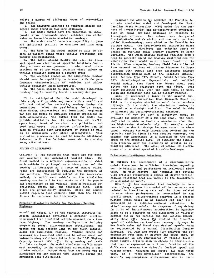
There are two main steps in the simulation process. Figure 1 shows a simplified diagram that illustrates the functional processing steps for the SOVT model. In the first step; three sets of data are input into the Speed-Headway Proqram. These data include traf­fic data (traffic volume, maximum headway, and vehicle composition), roadway data (length of simu-

24

Figure 1. Processing steps for SOVT model.

ROADWAY DATA

SPEED HEADWAY PROGRAM

VEHICLE QUEU ES

TRAFFIC SIMULATION PROGRAM

TRAFFIC OPERATION SUMMARY

TRAFFIC DATA

ROADWAY DATA

lation roadway, number of minor crossroads, and turning movements), and instructional data (simula­tion time and an initial random number). For each traffic lane, a headway distribution is generated in a manner that corresponds to the Schuhl model. The sequence of these headways is then arranged randomly to form an entering queue. Desired speed, which is generated by a normal d i stribution generator, and type of vehicle are assigned to each of the vehicles in the entering queue. One entering queue is gener­ated for each lane. These queues are then pooled into one entering queue according to entering time in chronological order. This queue is stored in a temporary file for later use.

In the second step, two types of data are input to the Traffic Simulation Program : (a) instruction data, including the number of times that simulation is to be repeated, the output printout interval, the maximum simulation time, the length of the simula­tion section, the throughput percentile speed for output data, and the number of no-passing zones, vertical grade sections, crossroads, speed-restric­tion zones, climbing lanes, and check stationsi and (b) roadway data, including the coordinates of speed-restriction zones, no-passing zones, vertical grades, turning zones, climbing lanes, crossroads, and check stations. Vehicle information, generated by the Speed-Headway Program, is read, and vehicles that have entering times equal to zero are placed on the simulation roadway and the clock is set xo zero. The program will proceed with the simulation routine until maximum simulation time is reached and the program is terminated. At each one of the user­defined output printout times, the program sum­mar izes and prints out speed-change cycles, headway distribution, speed distribution, passing and over­taking information, average traveling speed, travel time, instantaneous speed at every check station, and the instantaneous configuration of the traffic stream.

Transportation Research Record 806

By using FORTRAN H-level compiler, this model has been run on an IBM 370/165 computer. On an 8000-m (4.9-mile) roadway and with a simulation time of 3600 s, as traffic volume varies from 400 to 800 vehicles/h, the actual computer time varies from 28.3 to 62.3 s.

MODEL VALIDATION

The purpose of model validation is to verify that the computer model developed is so structured that the movement of vehicles on the simulation roadway approximates that of vehicles on an actual roadway. Because of financial limitations, no field data were collected to validate this model. Instead, a hypo­thetical 8000-m (26 250-ft) roadway section is used to check the reasonablene s s of simulation output. Different sets of data a re input i nto the model to simulate traffic flow. The results of these simula­tion runs are compared to verify that the model does indeed generate traffic-flow data that have a pat­tern similar to that normally found on actual high­ways. Four check stations are located at 1000, 3000 , 5000, ;:rnd 7000 m (3280, 9843, 16 404, and 22 966 ft), respectively, from the beginning of the roadway section.

Desired Speed Ve rsus Throughput Speed

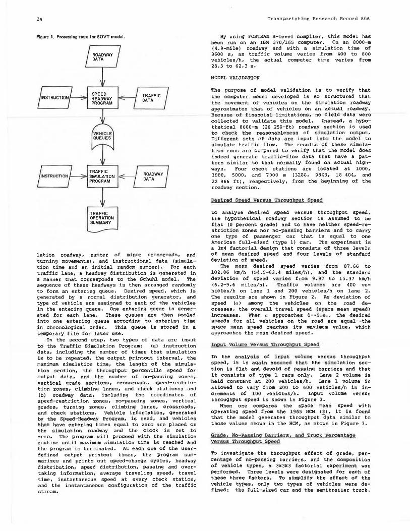
To analyze desired speed versus throughput speed, the hypothetical roadway section is assumed to be flat (0 percent grade) and to have neither speed-re­striction zones nor no-passing barriers a nd to carry one type of passenger c ar that is e qual to one American full-sized (type 1) car. The experiment is a 3x4 factorial design that consists of three levels of mean desired speed and four levels of standard deviation of speed.

The mean desired speed varies from 87.66 to 102.06 km/h (54.5-63.4 miles/h), and the standard deviation of speed varies from 9 . 97 to 15.37 km/h (6.2-9.6 miles/h). Traff ic volumes are 400 ve­hicles/h on lane 1 and 200 vehicles/h on lane 2. The results are shown in Figure 2. As deviation of speed (a) among the vehicles on the road de­creases, the overall travel speed (space mean speed) increases. When a approaches 0--i.e ., the desired speeds for all vehicles on the road are equal--the space mean speed reaches its maximum value, which approaches the mean desired speed.

Input Volume Versus Throug hput Speed

In the analysis of i nput vol ume ve i:sus throughput speed, it is again a ssumed that the simulation sec­tion is flat and devoid of passing barriers and that it consists of type 1 cars only. Lane 2 volume is held constant at 200 vehicles/h. Lane 1 volume is allowed to vary from 200 to 600 vehicles/h in in­crements of 100 vehicles/h. Input volume versus throughput speed is shown in Figure 3.

When one compares the space mean speed with operating speed from the 1965 HCM (3), it is found that the model generates throughput data similar to those values shown in the HCM, as shown in Figure 3.

Gr ade, No-Pass ing Barriers , and Truc k Pe rcent age Versus Throughput Speed

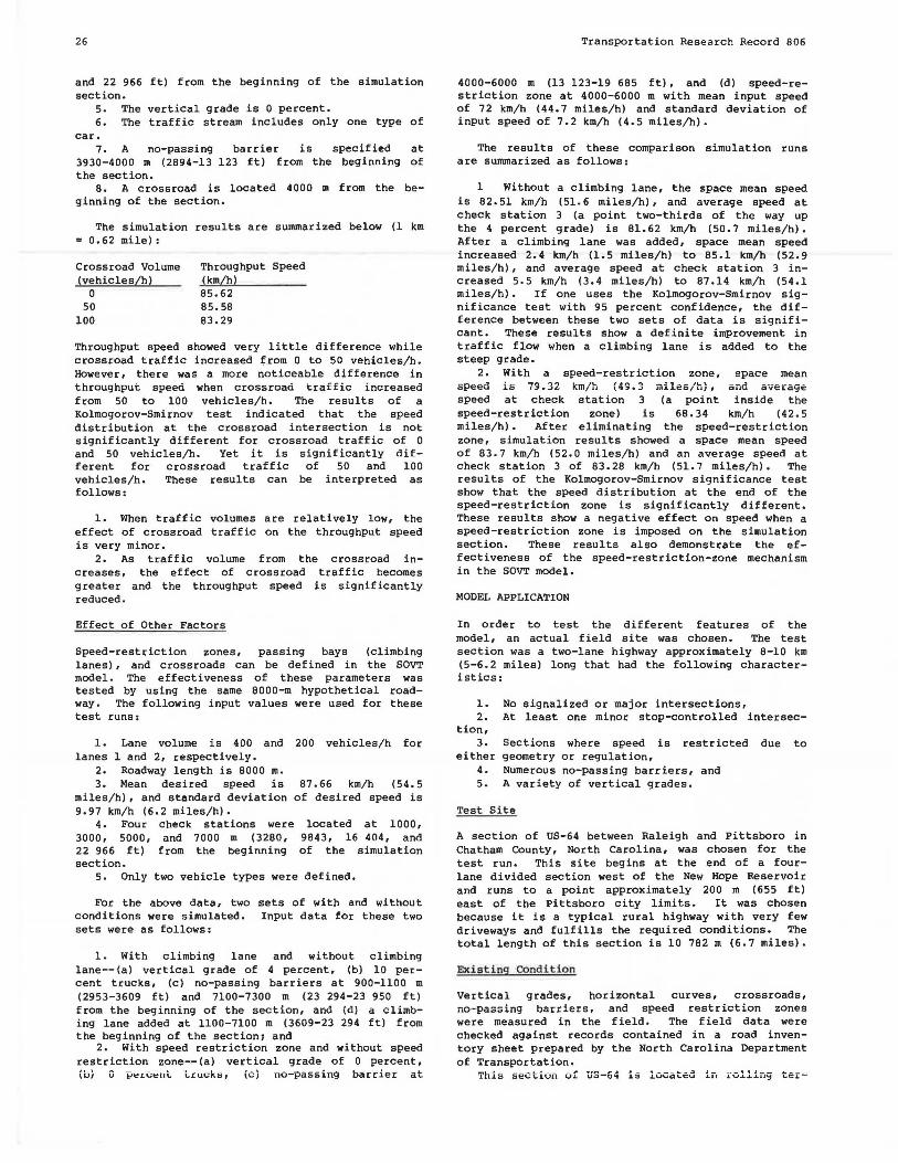
To investigate the throughput effect of grade, per­centage of no - passing barriers, and the composition of vehicle t ypes , a 3x3x3 factorial experiment was performed. Three levels were designated for each of these three factors. To simplify the effect of the vehicle types, only two types of vehicles were de­fined i the full-s ized car and the semitrailer truck.

Transportation Research Record 806

The three levels of vehicle composition of cars and trucks were 100 percent cars and 0 percent trucks, 95 percent cars and 5 percent trucks, and 90 percent cars and 10 percent trucks. The three levels of vertical grades were O, 2, and 4 percent, and the three levels of no-passing barriers were O, 20, and 40 percent. Input traffic volumes were held constant throughout these simulations. Lane 1 vol­ume was set at 400 vehicles/h and lane 2 volume at 200 vehicles/h. The results of these simulation runs are shown in Figure 4. From the middle and right-hand graphs, it is obvious that the interac­tions between grade and percentage of no-passing barriers and between percentage of no-passing bar-

Figure 2. Space mean throughput speed versus mean input speed.

IOO :I: ..... :i; ~

0 95 w w a.. en f--::::> a.. ::::> a: :I: f--

z <t

85 w :i;

w (.)

it en

eo

PRESET CONOITIONS, 0% GRADE

0% NO· PASSING 600 VPH

ONE TYPE OF VEHICLE

Note: 1 km = 0.62 mile.

85 90

CT= 0

er= STANDARD DEVIATION OF INPUT SPEED

95 100

MEAN INPUT SPEED (KM/H)

Figure 4. Space mean throughput speed versus (left) percentage of trucks and vertical grade, (middle) percentage of no-passing barriers and vertical grade, and (right) percentage of no-passing barriers and percentage of trucks.

85

::c i 80 ~

0

"" "" Bi 75 z

"' "" :IE

"" u

~ 70

• G=O%

·----.._, G=2°/o .

\ •G=4°/o

PERCENT TRUCKS

25

riers and percentage of trucks are minor. The left-hand graph shows that, as grades become steeper, the effect of truck percentage on through­put speed is greater. This can be explained by the restriction of truck acceleration capability due to steep grade.

Crossroad Traffic Volume Versus Throughput Speed

To investigate the effect of crossroad traffic, the same 8000-m hypothetical roadway is used. The fol­lowing input data are used for these test runs:

1. Lane volume is 400 and 200 vehicles/h for lanes 1 and 2, respectively.

2. The three levels of crossroad traffic volume are O, 50, and 100 vehicles/h.

3. Mean desired speed is 87.66 km/h (54.5 miles/h), and standard deviation of desired speed is 9.97 km/h (6.2 miles/h) on the main roadway.

4. Four internal check stations were located at 1000, 3950, 4050, and 7000 m (3280, 12 963, 13 283,

Figure 3. Input volume versus output speed.

C B5th PERCENTILE SPEED 0 SPACE MEAN SPEED

PRESET CONDITIONS, 0% GRADE 0°/o NO-PASSING ONE TYPE OF VEHICLE

Note: 1 km = 0.62 mile.

6 TIME MEAN SPEED - AT, END OF SIMULATION SECTION

x OPERATING SPEED - FROM "1965 HIGHWAY CAPACITY MANUAL

11

FIG. I0-2b PAGE 310

4 0

20 40 20 40 PERCENT NO PASSING ZONE PERCENT NO PASSING ZONE

26

and 22 966 ft) from the beginning of the simulation section.

5. The vertical grade is 0 percent. 6. The traffic stream includes only one type of

car. 7. A no-passing barrier is specified at

3930-4000 m (2894-13 123 ft) from the beginning of the section.

8. A crossroad is located 4000 m from the be­ginning of the section.

The simulation results are summarized below (1 km 0.62 mile):

Crossroad Volume (vehicles/h)

Throughput Speed (km/h)

0 so

100

85.62 85. 58 83.29

Throughput speed showed very little difference while crossroad traffic increased ~rom 0 to 50 vehicles/h. However, there was a more noticeable difference in throughput speed when crossroad traffic increased from 50 to 100 vehicles/h. The results of a Kolmogorov-Smirnov test indicated that the speed distribution at the crossroad intersection is not significantly different for crossroad traffic of 0 and 50 vehicles/h. Yet it is significantly dif­ferent for crossroad traffic of 50 and 100 vehicles/h. These results can be interpreted as follows:

1. When traffic volumes are relatively low, the effect of crossroad traffic on the throughput speed is very minor.

crossroad in­traff ic becomes

is significantly

2. As traffic volume from the creases, the effect of crossroad greater and the throughput speed reduced.

Effect of Other Factors

Speed-restriction zones, passing bays (climbing lanes), and crossroads can be defined in the SOVT model. The effectiveness of these parameters was tested by using the same 8000-m hypothetical road­way. The following input values were used for these test runs:

1. Lane volume is 400 and lanes l and 2, respectively.

2. Roadway length is 8000 m. 3. Mean desired speed is

miles/h) , and standard deviation 9.97 km/h (6.2 miles/h).

4. Four check stations were 3000, 5000, and 7000 m (3280, 22 966 ft) from the beginning section.

200 vehicles/h for

87. 66 km/h (54.5 of desired speed is

located at 1000, 9843, 16 404, and of the simulation

s. Only two vehicle types were defined.

For the above data, two sets of with and without conditions were simulated. Input data for these two sets were as follows:

1. With climbing lane and without climbing lane--(a) vertical grade of 4 percent, (b) 10 per­cent trucks, (c) no-passing barriers at 900-1100 m (2953-3609 ft) and 7100-7300 m (23 294-23 950 ft) from the beginning of the section, and (d) a climb­ing lane added at 1100-7100 m (3609-23 294 ft) from the beginning of the section: and

2. With speed restriction zone and without speed restriction zone--(a) vertical grade of O percent, (bj 0 percent trucks, (cj no-passing barrier at

Transportation Research Record 806

4000-6000 m (13 123-19 685 ft), and (d) speed-re­striction zone at 4000-6000 m with mean input speed of 72 km/h (44. 7 miles/h) and standard deviation of input speed of 7.2 km/h (4.5 miles/h).

The results of these comparison simulation runs are summarized as follows:

l Without a climbing lane, the space mean speed is 82.51 km/h (51.6 miles/h), and average speed at check station 3 (a point two-thirds of the way up the 4 percent grade) is BL 62 km/h (50. 7 miles/h). After a climbing lane was added, space mean speed increased 2.4 km/h (1.5 miles/h) to 85.l km/h (52.9 miles/h) , and average speed at check station 3 in­creased 5.5 km/h (3.4 miles/h) to 87.14 km/h (54.l miles/h). If one uses the Kolmogorov-Smirnov sig­nificance test with 95 percent confidence, the dif­ference between these two sets of data is signifi­cant. These results show a definite improvement in traffic flow when a climbing lane is added to the steep grade.

2. With a speed-restriction zone, space mean speed is 79.32 km/h (49.3 miles/h), and average speed at check station 3 (a point inside the speed-restriction zone) is 68.34 km/h (42.5 miles/h). After eliminating the speed-restriction zone, simulation results showed a space mean speed of 83.7 km/h (52.0 miles/h) and an average speed at check station 3 of 83.28 km/h (51.7 miles/h). The results of the Kolmogorov-Smirnov significance test show that the speed distribution at the end of the speed-restriction zone is significantly different. These results show a negative effect on speed when a speed-restriction zone is imposed on the simulation section. These results also demonstrate the ef­fectiveness of the speed-restriction-zone mechanism in the SOVT model.

MODEL APPLICATION

In order to test the different features of the model, an actual field site was chosen. The test section was a two-lane highway approximately 8-10 km (5-6. 2 miles) long that had the following character­istics:

1. No signalized or major intersections, 2. At least one minor stop-controlled intersec­

tion, 3. Sections where speed is restricted due to

either geometry or regulation, 4. Numerous no-passing barriers, and 5. A variety of vertical grades.

Test Site

A section of US-64 between Raleigh and Pittsboro in Chatham County, North Carolina, was chosen for the test run. This site begins at the end of a four­lane divided section west of the New Hope Reservoir and runs to a point approximately 200 m (655 ft) east of the Pittsboro city limits. It was chosen because it is a typical rural highway with very few driveways and fulfills the required conditions. The total length of this section is 10 782 m (6.7 miles).

Existing Condition

Vertical grades, horizontal curves, crossroads, no-passing barriers, and speed restriction zones were measured in the field. The field data were checked against records contained in a road inven­tory sheet prepared by the North Carolina Department of Transportation.

This section of US-64 is located in rolling teL~

Transportation Research Record 806

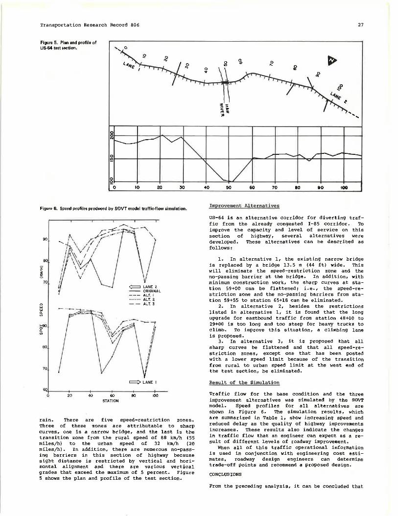
Figure 5. Plan and profile of US-64 test section.

27

.. .....

~1--~-t-~----f~~-+-~--t~--===t--.L~--+~~+-~--+-~~+-~-4--~~ 0 10 zo

Figure 6. Speed profiles produced by SOVT model traffic-flow simulation.

0

"' "' "-

"'

90

80

70

l;ilO Q.

VI

80

70

0

--... r.. ~ - _....._ --"\. " .r~:-- - - '\.

---.. J_ \ ,I/ I /~\/I / 1/'~ I / /1 \ ~ I \ I

I ' I f v' I

I

40 60 STATION

~LANE I

80 100

rain. There are five speed-restriction zones. Three of these zones are attributable to sharp curves, one is a narrow bridge, and the last is the transition zone from the rural speed of 88 km/h (55 miles/hl to the urban speed of 32 km/h ( 20 miles/h). In addition, there are numerous no-pass­ing barriers in this section of highway because sight distance is restricted by vertical and hori­zontal alignment and there are various vertical grades that exceed the maximum of 5 percent. Figure 5 shows the plan and profile of the test section.

40 60 70 10 10 100

Improvement Alternatives

US-64 is an alternative corridor for diverting traf­fic from the already congested I-85 corridor. To improve the capacity and level of service on this section of highway, several alternatives were developed. These alternatives can be described as follows:

1. In alternative 1, the existing narrow bridge is replaced by a bridge 13.5 m (44 ft) wide. This will eliminate the speed-restriction zone and the no-passing barrier at the bridge. In addition, with minimum construction work, the sharp curves at sta­tion 59+00 can be flattenedi i.e., the speed-re­striction zone and the no-passing barriers from sta­tion 59+55 to station 65+18 can be eliminated.

2. In alternative 2, besides the restrictions listed in alternative 1, it is found that the long upgrade for eastbound traffic from station 48+00 to 29+00 is too long and too steep for heavy trucks to climb. To improve this situation, a climbing lane is proposed.

3. In alternative 3, it is proposed that all sharp curves be flattened and that all speed-re­striction zones, except one that has been posted with a lower speed limit because of the transition from rural to urban speed limit at the west end of the test section, be eliminated.

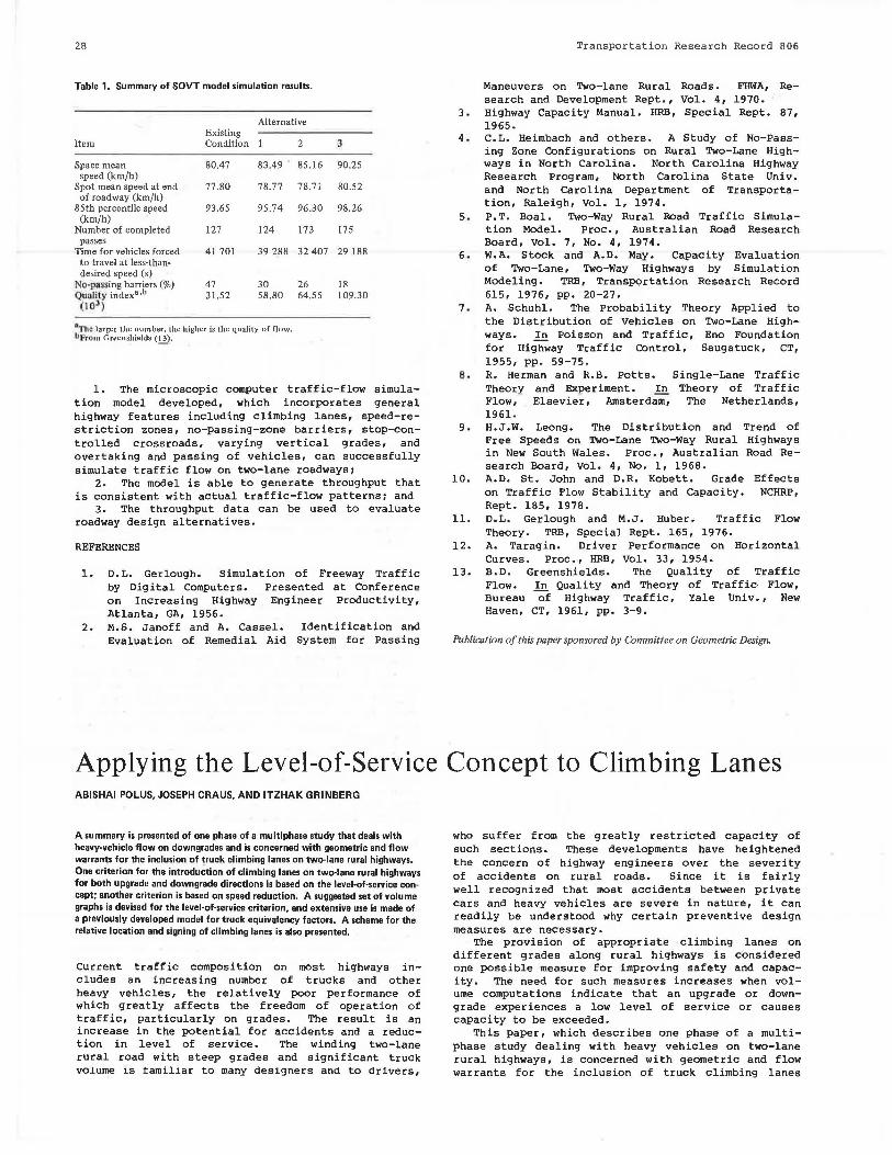
Result of the Simulation

Traffic flow for the base condition and the three improvement alternatives was simulated by the SOVT model. Speed profiles for all alternatives are shown in Figure 6. The simulation results, which are summarized in Table 1, show increasing speed and reduced delay as the quality of highway improvements increases. These results also indicate the changes in traffic flow that an engineer can expect as a re­sult of different levels of roadway improvement.

When all of this traffic operational information is used in conjunction with engineering cost esti­mates, roadway design engineers can determine trade-off points and recommend a proposed design.

CONCLUSIONS

From the preceding analysis, it can be concluded that

28

Table 1. Summary of SOVT model simulation results.

Item

Space mean speed (km/h)

Spot mean speed at end of road way (km/h)

85th percentile speed (km/h)

Number of completed passes

Time for vehicles forced to travel at less-than­desired speed (s)

No-passing barriers(%) Quality index• ,b

(!OJ)

Alternative Existing Condition 2 3

80.47 83.49 . 85.16 90.25

77 .80 78.77 78.71 80.52

93.65 95.74 96.30 98.26

127 124 173 175

41 701

47 31.52

39 288 32 407 29 188

30 26 18 58.80 64.55 109.30

*Tho. 1arger the number, the higher is the quality of flow. bf'rom Greenshields (£:>·

1. The microscopic computer traffic-flow simula­tion model developed, which incorporates general highway features including climbing lanes, speed-re­striction zones, no-passing-zone barriers, stop-con­trolled crossroads, varying vertical grades, and overtaking and passing of vehicles, can successfully simulate traffic flow on two-lane roadwaysi

2. The model is able to generate throughput that is consistent with actual traffic-flow patternsi and

3. The throughput data can be used to evaluate roadway design alternatives.

REFERENCES

1. D. L. Gerlough. Simulation of Freeway Traffic by Digital Computers. Presented at Conference on Increasing Highway Engineer Productivity, Atlanta, GA, 1956.

2. M.S. Janoff and A. Cassel. Identification and Evaluation of Remedial Aid System for Passing

Transportation Research Record 806

Maneuvers on Two-lane Rural Roads. FHWA, Re­search and Development Rept., Vol. 4, 1970.

3. Highway Capacity Manual. HRB, Special Rept. 87, 1965.

4 . C.L. Heimbach and others. A Study of No-Pass­ing Zone Configurations on Rural Two-Lane High­ways in North Carolina. North Carolina Highway Research Program, North Carolina State Univ. and North Carolina Department of Transporta­tion, Raleigh, Vol. 1, 1974.

5 . P.T. Boal. Two-Way Rural Road Traffic Simula­tion Model. Proc., Australian Road Research Board, Vol. 7, No. 4, 1974.

6. W.A. Stock and A.O. May. Capacity Evaluation of Two-Lane, Two-Way Highways by Simulation Modeling. TRB, Transportation Research Record 615, 1976, pp. 20-27.

7 . A. Schuh!. The Probability Theory Applied to the Distribution of Vehicles on Two-Lane High­ways. In Poisson and Traffic, Eno Foundation for Highway Traffic Control, Saugatuck, CT, 1955, pp. 59-75.

8. R. Herman and R.B. Potts. Single-Lane Traffic Theory and Exp eriment. In Theory of Traffic Flow, Elsevier, Amsterdam, The Netherlands, 1961.

9. H.J.W. Leong. The Distribution and Trend of Free Speeds on Two-Lane Two-Way Rural Highways in New South Wales. Proc., Australian Road Re­search Board, Vol. 4, No. 1, 1968.

10. A.O. St. John and D.R. Kobett. Grade Effects on Traffic Flow Stability and Capacity. NCHRP, Rept. 185, 1978.

11. D.L. Gerlough and M.J. Huber. Traffic Flow Theory. TRB, Special Rept. 165, 1976.

12. A. Taragin. Driver Performance on Horizontal Curves. Proc., HRB, Vol. 33, 1954.

13. B.D. Greenshields. The Quality of Traffic Flow. In Quality and Theory of Traffic Flow, Bureau of Highway Traffic, Yale Univ., New Haven, CT, 1961, pp. 3-9.

Publication of this paper sponsored by Committee on Geometric Design.

Applying the Level-of-Service Concept to Climbing Lanes ABISHAI POLUS, JOSEPH CRAUS, AND ITZHAK GRINBERG

A summary is presented of one phase of a multiphase study that deals with heavy-vehicle flow on downgrades and is concerned with geometric and flow warrants for the inclusion of truck climbing lanes on two-lane rural highways. One criterion for the introduction of climbing lanes on two-lane rural highways for both upgrade and downgrade directions is based on the level-of-service con­cept; another criterion is based on speed reduction. A suggested set of volume graphs is devised for the level-of-service criterion, and extensive use is made of a previously developed model for truck equivalency factors. A scheme for the relative location and signing of climbing lanes is also presented.

Current traffic composition on most highways in­cludes an increasing number of trucks and other heavy vehicles, the relatively poor performance of which greatly affects the freedom of operation of traffic, particularly on grades. The result is an increase in the potential for accidents and a reduc­tion in level of service. The winding two-lane rural road with steep grades and significant truck volume is familiar to many designers and to drivers,

who suffer from the greatly restricted capacity of such sections. These developments have heightened the concern of highway engineers over the severity of accidents on rural roads. Since it is fairly well recognized that most accidents between private cars and heavy vehicles are severe in nature, it can readily be understood why certain preventive design measures are necessary.

The provision of appropriate climbing lanes on different grades along rural highways is considered one possible measure for improving safety and capac­ity. The need for such measures increases when vol­ume computations indicate that an upgrade or down­grade experiences a low level of service or causes capacity to be exceeded.

This paper, which describes one phase of a multi­phase study dealing with heavy vehicles on two-lane rural highways, is concerned with geometric and flow warrants for the inclusion of truck climbing lanes