Simulation of fractional Brownian motion - Columbia Universityad3217/fbm/thesis.pdf · Simulation...
77
Simulation of fractional Brownian motion Ton Dieker [email protected] CWI P.O. Box 94079 1090 GB Amsterdam The Netherlands and University of Twente Department of Mathematical Sciences P.O. Box 217 7500 AE Enschede The Netherlands
Transcript of Simulation of fractional Brownian motion - Columbia Universityad3217/fbm/thesis.pdf · Simulation...
Simulation offractional Brownian motion
CWIP.O. Box 940791090 GB AmsterdamThe Netherlands
and
University of TwenteDepartment of Mathematical SciencesP.O. Box 2177500 AE EnschedeThe Netherlands

Preface
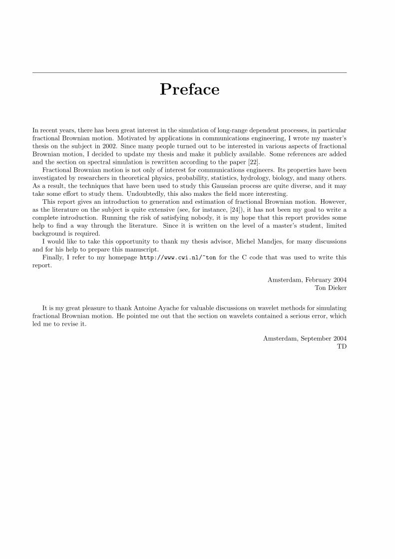
In recent years, there has been great interest in the simulation of long-range dependent processes, in particularfractional Brownian motion. Motivated by applications in communications engineering, I wrote my master’sthesis on the subject in 2002. Since many people turned out to be interested in various aspects of fractionalBrownian motion, I decided to update my thesis and make it publicly available. Some references are addedand the section on spectral simulation is rewritten according to the paper [22].
Fractional Brownian motion is not only of interest for communications engineers. Its properties have beeninvestigated by researchers in theoretical physics, probability, statistics, hydrology, biology, and many others.As a result, the techniques that have been used to study this Gaussian process are quite diverse, and it maytake some effort to study them. Undoubtedly, this also makes the field more interesting.
This report gives an introduction to generation and estimation of fractional Brownian motion. However,as the literature on the subject is quite extensive (see, for instance, [24]), it has not been my goal to write acomplete introduction. Running the risk of satisfying nobody, it is my hope that this report provides somehelp to find a way through the literature. Since it is written on the level of a master’s student, limitedbackground is required.
I would like to take this opportunity to thank my thesis advisor, Michel Mandjes, for many discussionsand for his help to prepare this manuscript.
Finally, I refer to my homepage http://www.cwi.nl/~ton for the C code that was used to write thisreport.
Amsterdam, February 2004Ton Dieker
It is my great pleasure to thank Antoine Ayache for valuable discussions on wavelet methods for simulatingfractional Brownian motion. He pointed me out that the section on wavelets contained a serious error, whichled me to revise it.
Amsterdam, September 2004TD

Contents
1 Introduction and motivation 1
1.1 A closer look at network traffic . . . . . . . . . . . . . . . . . . . . . . . . . . . . . . . . . . . . 11.1.1 Analysis of traffic traces . . . . . . . . . . . . . . . . . . . . . . . . . . . . . . . . . . . . 11.1.2 Self-similarity and long-range dependence . . . . . . . . . . . . . . . . . . . . . . . . . . 3
1.2 Fractional Brownian motion and fractional Gaussian noise . . . . . . . . . . . . . . . . . . . . . 41.2.1 Definitions and basic properties . . . . . . . . . . . . . . . . . . . . . . . . . . . . . . . . 51.2.2 Spectral densities . . . . . . . . . . . . . . . . . . . . . . . . . . . . . . . . . . . . . . . . 71.2.3 Another long-range dependent process . . . . . . . . . . . . . . . . . . . . . . . . . . . . 9
1.3 Implications for network models . . . . . . . . . . . . . . . . . . . . . . . . . . . . . . . . . . . . 101.4 Outline and scientific contribution . . . . . . . . . . . . . . . . . . . . . . . . . . . . . . . . . . 11
2 Simulation methods 13
2.1 Exact methods . . . . . . . . . . . . . . . . . . . . . . . . . . . . . . . . . . . . . . . . . . . . . 132.1.1 The Hosking method . . . . . . . . . . . . . . . . . . . . . . . . . . . . . . . . . . . . . . 132.1.2 The Cholesky method . . . . . . . . . . . . . . . . . . . . . . . . . . . . . . . . . . . . . 142.1.3 The Davies and Harte method . . . . . . . . . . . . . . . . . . . . . . . . . . . . . . . . 15
2.2 Approximate methods . . . . . . . . . . . . . . . . . . . . . . . . . . . . . . . . . . . . . . . . . 172.2.1 Stochastic representation method . . . . . . . . . . . . . . . . . . . . . . . . . . . . . . . 172.2.2 Aggregating packet processes . . . . . . . . . . . . . . . . . . . . . . . . . . . . . . . . . 172.2.3 (Conditionalized) Random Midpoint Displacement . . . . . . . . . . . . . . . . . . . . . 182.2.4 Spectral simulation, the Paxson method and the approximate circulant method . . . . . 192.2.5 Wavelet-based simulation . . . . . . . . . . . . . . . . . . . . . . . . . . . . . . . . . . . 242.2.6 Other methods . . . . . . . . . . . . . . . . . . . . . . . . . . . . . . . . . . . . . . . . . 27
Appendix: Proof of ξ(`)n → ξn in L2 . . . . . . . . . . . . . . . . . . . . . . . . . . . . . . . . . . . . . 29
3 Estimation and testing 31
3.1 Estimation . . . . . . . . . . . . . . . . . . . . . . . . . . . . . . . . . . . . . . . . . . . . . . . 313.1.1 Aggregated variance method . . . . . . . . . . . . . . . . . . . . . . . . . . . . . . . . . 313.1.2 Absolute moments method . . . . . . . . . . . . . . . . . . . . . . . . . . . . . . . . . . 333.1.3 Discrete variations . . . . . . . . . . . . . . . . . . . . . . . . . . . . . . . . . . . . . . . 333.1.4 The Higuchi method . . . . . . . . . . . . . . . . . . . . . . . . . . . . . . . . . . . . . . 343.1.5 Periodogram method . . . . . . . . . . . . . . . . . . . . . . . . . . . . . . . . . . . . . . 343.1.6 Variance of the regression residuals . . . . . . . . . . . . . . . . . . . . . . . . . . . . . . 363.1.7 R/S analysis . . . . . . . . . . . . . . . . . . . . . . . . . . . . . . . . . . . . . . . . . . 363.1.8 Whittle’s method . . . . . . . . . . . . . . . . . . . . . . . . . . . . . . . . . . . . . . . . 383.1.9 Wavelet method . . . . . . . . . . . . . . . . . . . . . . . . . . . . . . . . . . . . . . . . 38
3.2 Testing . . . . . . . . . . . . . . . . . . . . . . . . . . . . . . . . . . . . . . . . . . . . . . . . . 403.2.1 A goodness-of-fit test for the spectral density . . . . . . . . . . . . . . . . . . . . . . . . 403.2.2 A chi-square test for fractional Gaussian noise . . . . . . . . . . . . . . . . . . . . . . . 41
4 Evaluation of approximate simulation methods 43
4.1 Error analysis . . . . . . . . . . . . . . . . . . . . . . . . . . . . . . . . . . . . . . . . . . . . . . 434.1.1 The approximate circulant method . . . . . . . . . . . . . . . . . . . . . . . . . . . . . . 444.1.2 The RMDl,r method . . . . . . . . . . . . . . . . . . . . . . . . . . . . . . . . . . . . . . 484.1.3 The wavelet method . . . . . . . . . . . . . . . . . . . . . . . . . . . . . . . . . . . . . . 51
4.2 Stationarity and covariance analysis . . . . . . . . . . . . . . . . . . . . . . . . . . . . . . . . . 524.3 Testing the approximate samples . . . . . . . . . . . . . . . . . . . . . . . . . . . . . . . . . . . 57
4.3.1 The goodness-of-fit test for the spectral density . . . . . . . . . . . . . . . . . . . . . . . 57
4.3.2 The chi-square test . . . . . . . . . . . . . . . . . . . . . . . . . . . . . . . . . . . . . . . 584.4 Long-range dependence in approximate samples . . . . . . . . . . . . . . . . . . . . . . . . . . . 58
4.4.1 The Wilcoxon test . . . . . . . . . . . . . . . . . . . . . . . . . . . . . . . . . . . . . . . 604.4.2 The Freund-Ansari-Bradley test . . . . . . . . . . . . . . . . . . . . . . . . . . . . . . . 604.4.3 Estimation of H for the approximate methods . . . . . . . . . . . . . . . . . . . . . . . 61
4.5 Time complexity analysis . . . . . . . . . . . . . . . . . . . . . . . . . . . . . . . . . . . . . . . 64
5 Conclusions 67
Bibliography 69

CHAPTER 1
Introduction and motivation
Queueing theory plays an important role in the design of telecommunication networks. Classical queueingmodels often give insightful results, for example on (long-term) delays, packet losses, and buffer contentdistributions. However, research has shown that the assumptions in traditional models are not valid insome cases. Unfortunately, these cases are particularly important for data communication networks. Thoseassumptions concern mainly the arrival process of data packets.
In this report, we will study a random process, fractional Brownian motion, that models the arrivals ofnetwork packets better than classical models (at least for some types of traffic), but is parsimonious in thesense that only few parameters describe its statistical behavior. Research has shown that the use of fractionalBrownian motion instead of a traditional model has impact on queueing behavior; it affects several aspectsof queueing theory (e.g., buffer sizing, admission control and congestion control). The use of conventionalmodels (e.g., Poisson-type models) results in optimistic performance predictions and an inadequate networkdesign.
Since traditional models have extensively been studied in the past decades, relatively much is knownabout their properties, although there are still many open problems. In contrast, few theoretical results existfor queueing models based on fractional Brownian motion. Simulation studies that make use of generatedfractional Brownian motion traces are therefore of crucial importance, especially for complex queueing systems.
It is the aim of this report to evaluate several simulation methods for fractional Brownian motion. Althoughsome methods that simulate fractional Brownian motion are known, methods that simulate this process‘approximately’ have been proposed to reduce the computation time. Therefore, we will focus on the questionin what respect the approximate differ from exact samples.
In this first chapter, we start with the analysis of real network traffic traces to clarify that conventionalassumptions do not hold. Thereafter, we define fractional Brownian motion and study its basic properties.In Section 1.3, we get some feeling for the impact of the use of fractional Brownian motion in a teletrafficframework by studying a simple but insightful queueing model. Section 1.4 outlines this report, and addressesits scientific contribution.
1.1 A closer look at network traffic
1.1.1 Analysis of traffic traces
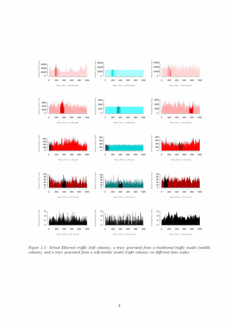
Willinger et al. [57] have analyzed high-quality Local Area Network (LAN) Ethernet traces. During morethan one day, every 10 milliseconds was measured how many packets and bytes passed the monitoring systemat Bellcore Research. (Data is sent in packets of bytes across the network.)
By studying the data, the authors find arguments for the presence of so-called self-similarity and long-range dependence. Before giving definitions, we will make this intuitively clear by the plots in Figure 1.1,which are taken from [57]. Starting with a time unit of 100 seconds (the upper row), each subsequent row isobtained from the previous one by increasing the time resolution by a factor of 10 and by concentrating ona randomly chosen subinterval, indicated by a shade. The lower row corresponds to the finest time scale (10milliseconds). The plots are made for actual Ethernet traffic (left column), a synthetic trace generated froma Poisson-type traffic model (middle column), and a synthetic trace generated from an appropriately chosenself-similar traffic model with a single parameter (right column). For a given time resolution (or, equivalently,interval length), the number of data packets arriving in each interval is computed and depicted as tiny bins.
1
0 200 400 600 800 1000
0
20000
40000
60000
0 200 400 600 800 1000
0
20000
40000
60000
0 200 400 600 800 1000
0
20000
40000
60000
0 200 400 600 800 1000
0
2000
4000
6000
0 200 400 600 800 1000
0
2000
4000
6000
0 200 400 600 800 1000
0
2000
4000
6000
0 200 400 600 800 1000
0200 400 600 800
0 200 400 600 800 1000
0
200
400
600
800
0 200 400 600 800 1000
0
200
400
600
800
0 200 400 600 800 1000
020406080
100
0 200 400 600 800 1000
020406080
100
0 200 400 600 800 1000
020 40 60 80 100
0 200 400 600 800 1000
0
5
10
15
0 200 400 600 800 1000
0
5
10
15
0 200 400 600 800 1000
0
5
10
15PSfrag replacements
Packets/T
ime
Unit
Packets/T
ime
Unit
Packets/T
ime
Unit
Packets/T
ime
Unit
Packets/T
ime
Unit
Packets/T
ime
Unit
Packets/T
ime
Unit
Packets/T
ime
Unit
Packets/T
ime
Unit
Packets/T
ime
Unit
Packets/T
ime
Unit
Packets/T
ime
Unit
Packets/T
ime
Unit
Packets/T
ime
Unit
Packets/T
ime
Unit
Time Unit = 100 SecondsTime Unit = 100 SecondsTime Unit = 100 Seconds
Time Unit = 10 SecondsTime Unit = 10 SecondsTime Unit = 10 Seconds
Time Unit = 1 SecondTime Unit = 1 SecondTime Unit = 1 Second
Time Unit = 0.1 SecondTime Unit = 0.1 SecondTime Unit = 0.1 Second
Time Unit = 0.01 SecondTime Unit = 0.01 SecondTime Unit = 0.01 Second
Figure 1.1: Actual Ethernet traffic (left column), a trace generated from a traditional traffic model (middlecolumn), and a trace generated from a self-similar model (right column) on different time scales.
2
Apart from the upper left plot, which suggests the presence of a daily cycle (the LAN is observed for 27hours), the plots in the left column look ‘similar’ in distributional sense: it is not possible to determine whatthe time unit is used by just looking at the shape of the plotted bins.
However, for a conventional model as in the middle column of Figure 1.1 (a batch Poisson model wassimulated to generate the traffic), the number of packets per bin has a very low standard deviation at thecoarsest time scale: the plot looks like a solid bar. By increasing the resolution, more ‘randomness’ shows up.This is caused by the fact that (independent) interarrival and service times have finite variance in traditionalqueueing models, e.g., exponential or Erlang distributions. The amount of traffic in disjoint time intervals isthen mutual independent if the size of the intervals is large enough. We will make the limiting behavior moreprecise for an (ordinary) Poisson arrival process in Section 1.3. Note that the plots in the middle column looksignificantly different from those in the left column.
On the contrary, the plots in the right column (generated by a self-similar model) are visually almostindistinguishable from those in the left column. The only clear difference is that in the upper plot nocyclical behavior is present. However, when desirable, this daily behavior can be incorporated by addingsome deterministic or stochastic trend.
We cannot just rely on one specific network trace of 27 hours to state that all LAN network traffic isself-similar. Therefore, Willinger et al. also study traces that are observed in other months and in a differentnetwork layout, making their conclusions more robust.
In another paper, Willinger et al. [58] tried to explain the self-similar nature of Ethernet LAN trafficby studying the source level, i.e., looking at the activity of all possible source-destination pairs in the LAN.They assume that each such pair is either sending bytes (‘ON’) or inactive (‘OFF’), where the ON- andOFF-periods strictly alternate. It is assumed that the lengths of the ON- and OFF-periods are independentand identical distributed (i.i.d.) and that all ON- and OFF-periods are also independent from one another.The authors find that the so-called ‘Noah Effect’ (high variability) can explain in some sense the self-similarphenomena that are observed on the aggregate level. The Noah effect is synonymous with infinite variance;it was empirically observed that many naturally occurring phenomena can well be described by distributionswith infinite variance. The authors study the cumulative amount of packets (or bytes) when many sourcesare present. When this Noah effect is present in the ON- or OFF-periods, the cumulative amount of packets(after rescaling time) is described by a simple transformation of fractional Brownian motion.
The same self-similar behavior as in LAN Ethernet traffic is also discovered in wide area networks (WANs)[40], variable bit rate (VBR) video [10], etc. Many work is going on to show its presence in different kinds ofdata traffic.
1.1.2 Self-similarity and long-range dependence
We will now make mathematically precise what we mean by self-similarity and long-range dependence. Itwill be no surprise that these two concepts are related to fractional Brownian motion, but we will first definethem in the framework of general stationary stochastic processes.
Let X = Xk : k = 0, 1, 2, . . . be a stationary discrete-time stochastic process, meaning that the vectors(Xk1
, . . . , Xkd) and (Xk1+n, . . . , Xkd+n) have the same distribution for all integers d, n ≥ 1 and k1, . . . , kd ≥ 0.
For Gaussian processes, it is equivalent to require that γ(k) := Cov(Xn, Xn+k) does not depend on n. Thesetwo notions are sometimes referred to as strict stationarity and second-order stationarity, respectively. Thefunction γ(·) is called the autocovariance function.
In Figure 1.1, we saw that summing up the amount of packets in the first 10 bins gives (up to scale) thesame plot in distributional sense. This is also valid for the next 10 bins and so on. Suppose that this reasoningapplies to a general factor m ≥ 1, not necessarily a power of 10. Mathematically, we then have for everyk ≥ 0,
Xkm + . . .+X(k+1)m−1 = amXk, (1.1)
where the equality is in the sense of equality in distribution. Although the scaling factor am > 0 is still not
defined by this intuitive reasoning, we first define a new process X (m) = X(m)k : k = 0, 1, 2, . . . for every
m ≥ 1:
X(m)k =
1
m
(
Xkm + . . .+X(k+1)m−1
)
.
Following Cox [16], we call a discrete-time stochastic process X self-similar with Hurst parameter 0 <H < 1 if X and m1−HX(m) have the same finite-dimensional distributions for all m ≥ 1. This means that forevery d ≥ 1 and 0 ≤ k1 < . . . < kd the vector
(Xk1, . . . , Xkd
)
3
has the same distribution as the vector
(m1−HX(m)k1
, . . . ,m1−HX(m)kd
),
implying that the correlation function r(·) = γ(·)/Var(X1) of X equals de correlation function r(m)(·) of X(m)
for all m. Thus, (1.1) holds with am = mH if X is self-similar with Hurst parameter H.The above definitions can easily be extended to continuous-time stochastic processes. A continuous-time
stochastic process Y = Y (t) : 0 ≤ t < ∞ is called self-similar with Hurst parameter 0 < H < 1 ifY (at) : 0 ≤ t <∞ and aHY (t) : 0 ≤ t <∞ have identical finite-dimensional distributions for all a > 0.
Weaker notions than self-similarity also exist. A process is second-order self-similar if the finite dimensionaldistributions of X and m1−HX(m) have equal mean and covariance structure. If this is only true as m→ ∞,the process is called asymptotically second-order self-similar, see [16].
Next we introduce the definition of long-range dependence. A stationary discrete-time processes X issaid to be a process with long-range dependence, long memory, or strong dependence when its autocovariancefunction γ(·) decays so slowly that
∑∞k=0 γ(k) = ∞ (in contrast to processes with summable covariances,
which are called processes with short-range dependence, short memory, or weak dependence). Intuitively,when long-range dependence is present, high-lag correlations may be individually small, but their cumulativeeffect is significant.
As pointed out by Beran [9], such a covariance structure has an important impact on usual statisticalinference. As an example, assume we have n observations of some random variable X with finite variance.The standard deviation of the mean is then proportional to n1/2 if the observations are uncorrelated. If thecovariances decay exponentially (as is the case with a so-called AR(1) process), the covariances are summableand similar behavior is observed: the standard deviation of the mean is proportional to n1/2 for sufficientlylarge n, although the proportionality constant is different. Suppose, on the other hand, that the covariancefunction γ(·) decays hyperbolically:
γ(k) ∼ cγ |k|−α (1.2)
as |k| tends to infinity for some 0 < α < 1 and a finite positive constant cγ . [In this report, we followthe notational convention that f(x) ∼ g(x) as x → X ∈ [−∞,∞] stands for limx→X f(x)/g(x) = 1.] It isreadily checked that the process is long-range dependent if (1.2) holds. Under this long-range dependence,the standard deviation of the mean is proportional to n−α/2! Of course, this affects confidence intervals forthe mean of X and all related test statistics. Moreover, the standard estimator for the variance of X becomesbiased. This bias does not disappear when the sample size increases, as is the case for short-range dependentprocesses.
It is important to note that Equation (1.2) determines only the decay of the correlations. It is very wellpossible that there are some specific lags for which γ(k) is particularly large, which makes the detectingof long-range dependence more difficult. In fact, it is theoretically impossible to conclude that long-rangedependence is present in a finite sample.
In general, self-similarity and long-range dependence are not equivalent. As an example, the incrementsof a standard Brownian motion are self-similar with Hurst parameter H = 1/2, but clearly not long-rangedependent (the increments are even independent). However, under the restriction 1/2 < H < 1, long-rangedependence is equivalent to asymptotic second-order self-similarity for stationary processes.
Before investigating the influence of fractional Brownian motion in a queueing framework, we will firstdefine this process and derive its basic properties.
1.2 Fractional Brownian motion and fractional Gaussian noise
Since we will shortly see that fractional Brownian motion is a Gaussian process, its covariance structure isone of its most important features. Therefore, the key subjects of this section are the covariance structure offractional Brownian motion and its incremental process, fractional Gaussian noise. Moreover, the propertiesof fractional Gaussian noise in the so-called frequency domain are described. Finally, another long-rangedependent process is presented for later use.
4

1.2.1 Definitions and basic properties
Fractional Brownian motion
In the pioneering work by Mandelbrot and van Ness [42], fractional Brownian motion is defined by its stochasticrepresentation
BH(t) :=1
Γ(H + 12 )
(∫ 0
−∞
[(t− s)H−1/2 − (−s)H−1/2]dB(s) +
∫ t
0
(t− s)H−1/2dB(s)
)
, (1.3)
where Γ represents the Gamma function Γ(α) :=∫∞
0xα−1 exp(−x)dx and 0 < H < 1 is called the Hurst
parameter (we soon see the connection with the Hurst parameter for self-similar processes). The integratorB is a stochastic process, ordinary Brownian motion. Note that B is recovered by taking H = 1/2 in(1.3). For later use, we assume that B is defined on some probability space (Ω,F , P ). We remark that thisrepresentation in terms of an integral with respect to Brownian motion is non-unique; see, e.g., p. 140 of [52]for a different representation. One point should be clarified in more detail: how to interpret an integral withrandom integrator B.
The notation suggests that this integral can be seen as a Lebesgue-Stieltjes integral. One could thereforethink that the integral can pathwise be computed in a Lebesgue-Stieltjes sense (recall that B can be regardedas a random function). However, this is impossible, since the paths of Brownian motion are highly irregular.For example, though the trajectories are continuous, they are almost surely non-differentiable and, moreimportantly in this case, the paths do not have bounded variation with probability 1. This property preventsus from calculating the integral as a pathwise Lebesgue-Stieltjes integral.
Having observed this, we have still not solved the interpretation problem. In fact, the integral is a so-calledstochastic integral with respect to usual Brownian motion. We will briefly explain its definition, but we willomit many details. For details on stochastic integration, the reader is referred to one of the many textbookson stochastic calculus, e.g., Karatzas and Shreve [37].
Avoiding technicalities caused by an unbounded integration interval, we will only discuss the definition ofthe stochastic integral
∫ b
a
φ(s)dB(s)
for finite a and b. This integral has a natural definition when the integrand φ is a so-called simple function,which means that there exists an integer ` > 0 and a strictly increasing sequence of real numbers (tj)
`j=0 with
t0 = a and t` = b, as well as a sequence of real numbers (φj)`−1j=0 such that φ(s) can be written as φ(s) = φj
for s ∈ (tj , tj+1] (the value at a turns out to have no influence). For such a simple function φ, the stochasticintegral has the following natural definition:
∫ b
a
φ(s)dB(s) =`−1∑
j=0
φj(B(tj+1) −B(tj)). (1.4)
A sequence of (Lebesgue) square integrable functions (ψn) is said to converge in L2–norm to a squareintegrable function ψ if
limn→∞
∫
(ψ(s) − ψn(s))2ds = 0.
The integration interval is again [a, b], which is sometimes made explicit by calling this convergence inL2([a, b])–norm. It is known that every square integrable function can be written as a limit in L2–normof a sequence of simple functions. Assume therefore that ψn is a simple function for every n. A possibledefinition for
∫
ψ(s)dB(s) would be limn→∞
∫
ψn(s)dB(s). Unfortunately, this limit only exists almost surelywhen ψ satisfies very restrictive conditions.
Since∫ b
aψn(s)dB(s) has a finite second moment, it is known that there exists a square integrable random
variable Z on our probability space (Ω,F , P ) with the property
limn→∞
E
(
Z −∫ b
a
ψn(s)dB(s)
)2
= 0, (1.5)
where E denotes the expectation operator with respect to P . This random variable Z is sometimes referredto as the L2 limit of approximating stochastic integrals of simple functions, and the type of convergence iscalled convergence in L2–norm (note the subtle difference in notation with the previous L2–norm). If ψ issquare integrable, this random variable is unique in the sense that another random variable that satisfies (1.5)
5
is almost sure equal to Z. This makes it possible to take this Z as the definition of the stochastic integral∫
ψ(s)dB(s). Moreover, it can be shown that Z is independent of the approximating sequence (ψn)n, implyingthat if a given sequence of simple functions (ψn)n converges in L2–norm to ψ, the corresponding sequence ofstochastic integrals
(∫
ψn(s)dB(s))
nconverges in L2–norm to
∫
ψ(s)dB(s). We will use this fact in Chapter2.
Note that∫
ψ(s)dB(s) is only defined for square integrable ψ by this reasoning. The integral Z is writtenas∫
ψ(s)dB(s), but it has nothing to do with other types of integrals with the same notation, althoughsome of the usual properties of integrals are shared, e.g., linearity. Also note that some specific properties ofBrownian motion are used in the way we defined the stochastic integral. Extensions to other processes arepossible using the same arguments, although the definition of the stochastic integral is still a topic of researchfor interesting processes that do not fit in this framework.
Omitting details, the second moments of the stochastic integral in (1.3) can be computed by a standardformula, which leads to the fact that the variance of BH(t) is VHt
2H for some constant VH . From now on,we will always assume that we deal with normalized (or standardized) fractional Brownian motion, which hasexactly variance t2H . We will use the same notation for the normalized process as before.
A normalized fractional Brownian motion BH = BH(t) : 0 ≤ t < ∞ with 0 < H < 1 is uniquelycharacterized by the following properties, cf., e.g., [45]:
• BH(t) has stationary increments;
• BH(0) = 0, and EBH(t) = 0 for t ≥ 0;
• EB2H(t) = t2H for t ≥ 0;
• BH(t) has a Gaussian distribution for t > 0.
We always suppose that we deal with a version of BH with continuous sample paths (such a version exists bythe Kolmogorov criterion for continuity of sample paths). From the first three properties it follows that thecovariance function is given by
ρ(s, t) = EBH(s)BH(t) =1
2
t2H + s2H − (t− s)2H
(1.6)
for 0 < s ≤ t. For Gaussian processes, the mean and covariance structure determine the finite-dimensionaldistributions uniquely. Therefore, we conclude from (1.6) that BH(at) : 0 ≤ t <∞ and aHBH(t) : 0 ≤ t <∞ have the same finite-dimensional distributions: fractional Brownian motion with Hurst parameter H isself-similar with Hurst parameter H. In fact, fractional Brownian motion is the only Gaussian process withstationary increments that is self-similar [16].
Besides communications engineering, fractional Brownian motion has applications in other areas, such asfinance, physics, and bioengineering, to name but a few. In bioengineering for instance, fractional Brownianmotion is used to model regional flow distributions in the heart, the lung and the kidney [7].
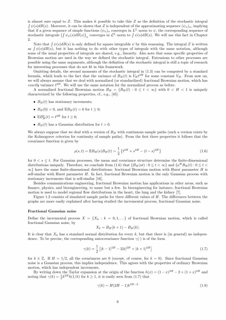
Figure 1.2 consists of simulated sample paths for three different values of H. The differences between thegraphs are more easily explained after having studied the incremental process, fractional Gaussian noise.
Fractional Gaussian noise
Define the incremental process X = Xk : k = 0, 1, . . . of fractional Brownian motion, which is calledfractional Gaussian noise, by
Xk = BH(k + 1) −BH(k).
It is clear that Xk has a standard normal distribution for every k, but that there is (in general) no indepen-dence. To be precise, the corresponding autocovariance function γ(·) is of the form
γ(k) =1
2
[
|k − 1|2H − 2|k|2H + |k + 1|2H]
(1.7)
for k ∈ Z. If H = 1/2, all the covariances are 0 (except, of course, for k = 0). Since fractional Gaussiannoise is a Gaussian process, this implies independence. This agrees with the properties of ordinary Brownianmotion, which has independent increments.
By writing down the Taylor expansion at the origin of the function h(x) = (1− x)2H − 2 + (1 + x)2H andnoting that γ(k) = 1
2k2Hh(1/k) for k ≥ 1, it is easily seen from (1.7) that
γ(k) ∼ H(2H − 1)k2H−2 (1.8)
6
0 200 400 600 800 1000−6
−4−2
02
4
0 200 400 600 800 1000
020
4060
0 200 400 600 800 1000
−200
−100
050
PSfrag
replacem
ents
H=
0.2
H=
0.5
H=
0.8
Figure 1.2: Samples of fractional Brownian motion for H = 0.2, H = 0.5 and H = 0.8.
as k → ∞. This implies long-range dependence for 1/2 < H < 1:∑∞
k=0 γ(k) = ∞. It is important to knowthat the measurements on real traffic traces indeed suggest that 1/2 < H < 1, see [57].
Since we have noted that long-range dependence is closely related to self-similarity for 1/2 < H < 1, itis natural to study whether fractional Gaussian noise is also a self-similar process. To make sure that thisis indeed the case, it suffices to show that mX(m) and mHX have the same finite-dimensional distributions.Since we have already seen that fractional Brownian motion is self-similar, the following holds:
Cov(Xkm + . . .+X(k+1)m−1, Xlm + . . .+X(l+1)m−1)
= Cov(BH((k + 1)m) −BH(km), BH((l + 1)m) − BH(lm))?= Cov(mH(BH(k + 1) −BH(k)),mH(BH(l + 1) −BH(l)))
= Cov(mHXk,mHXl).
At the equality?=, we used the fact that the vectors (BH(mk), BH(m(k + 1)), BH(ml), BH(m(l + 1))) and
(mHBH(k),mHBH(k + 1),mHBH(l),mHBH(l + 1)) have the same distribution for k 6= l, because all finite-dimensional (particularly four-dimensional) distributions are equal (since fractional Brownian motion is self-similar). A similar argument shows that this is also the case for k = l. Because of the normality, it suffices tohave equal means and covariances to conclude that the finite-dimensional distributions of mX (m) and mHXare equal: fractional Gaussian noise is self-similar.
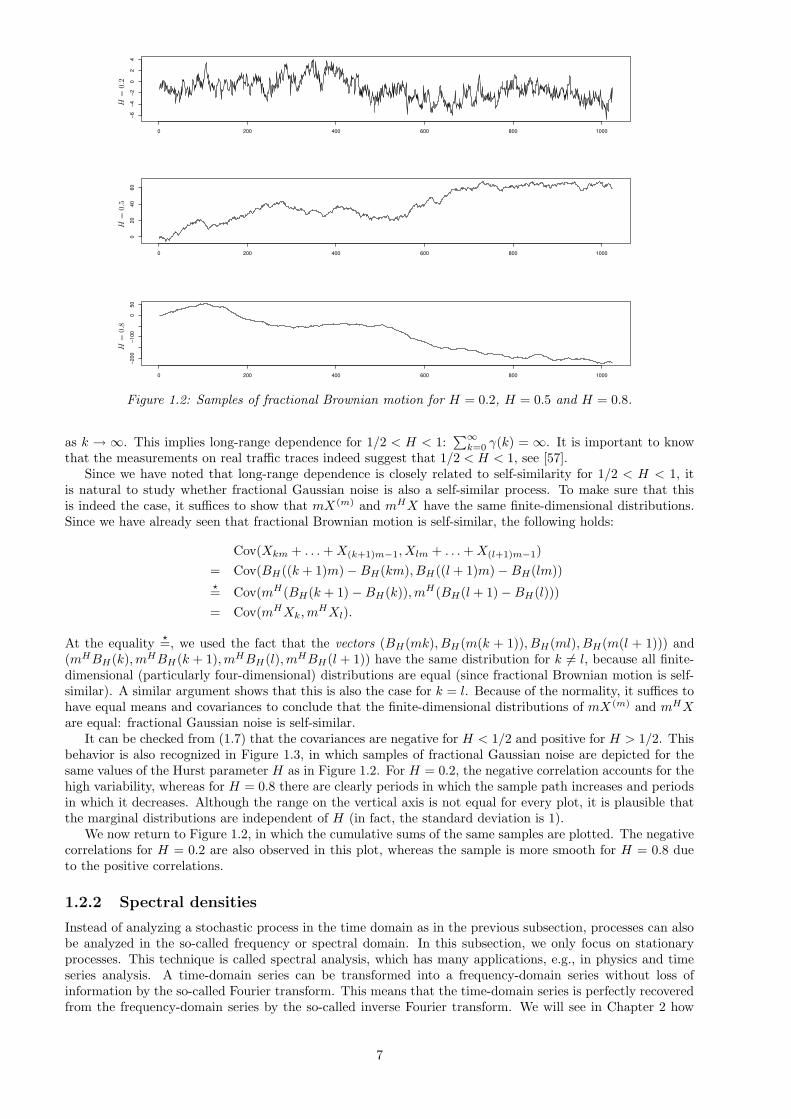
It can be checked from (1.7) that the covariances are negative for H < 1/2 and positive for H > 1/2. Thisbehavior is also recognized in Figure 1.3, in which samples of fractional Gaussian noise are depicted for thesame values of the Hurst parameter H as in Figure 1.2. For H = 0.2, the negative correlation accounts for thehigh variability, whereas for H = 0.8 there are clearly periods in which the sample path increases and periodsin which it decreases. Although the range on the vertical axis is not equal for every plot, it is plausible thatthe marginal distributions are independent of H (in fact, the standard deviation is 1).
We now return to Figure 1.2, in which the cumulative sums of the same samples are plotted. The negativecorrelations for H = 0.2 are also observed in this plot, whereas the sample is more smooth for H = 0.8 dueto the positive correlations.
1.2.2 Spectral densities
Instead of analyzing a stochastic process in the time domain as in the previous subsection, processes can alsobe analyzed in the so-called frequency or spectral domain. In this subsection, we only focus on stationaryprocesses. This technique is called spectral analysis, which has many applications, e.g., in physics and timeseries analysis. A time-domain series can be transformed into a frequency-domain series without loss ofinformation by the so-called Fourier transform. This means that the time-domain series is perfectly recoveredfrom the frequency-domain series by the so-called inverse Fourier transform. We will see in Chapter 2 how
7
0 200 400 600 800 1000
−3−1
01
23
0 200 400 600 800 1000
−20
24
0 200 400 600 800 1000
−3−1
01
23
PSfrag
replacem
ents
H=
0.2
H=
0.5
H=
0.8
Figure 1.3: Samples of fractional Gaussian noise for H = 0.2, H = 0.5 and H = 0.8.
‘approximate’ fractional Brownian motion can be simulated by generating a frequency-domain sample andthen transforming the resulting series. The required theoretical background is described in this subsection.
Fourier proved that a (deterministic) periodic function can be written as a unique linear combination oftrigonometric functions with different frequencies, making it thus possible to describe this function completelyby the amount in which each frequency is present. It is possible and useful to extend this idea to non-periodicfunctions; a deterministic function (or a realization of a stochastic process) can be thought to consist oftrigonometric functions with different frequencies. The information to which extend each frequency is presentin the signal is then summarized in the so-called spectral density, also called power spectrum density becauseof its interpretation in physics.
When analyzing stochastic processes in a frequency framework, it is impossible to study every realizationindividually. However, it turns out (see, e.g., [51]) that for stationary processes the expected frequencyinformation is contained in the autocovariance function.
For stationary stochastic processes, the spectral density is computed as follows for frequencies −π ≤ λ ≤ π:
f(λ) =
∞∑
j=−∞
γ(j) exp(ijλ), (1.9)
where γ(·) again denotes the autocovariance function. The autocovariance function is recovered by the inver-sion formula
γ(j) =1
2π
∫ π
−π
f(λ) exp(−ijλ)dλ. (1.10)
In this report, we are particularly interested in the spectral density of fractional Gaussian noise. It can beseen [9] that this density is given by
f(λ) = 2 sin(πH)Γ(2H + 1)(1 − cosλ)[
|λ|−2H−1 +B(λ,H)]
, (1.11)
with
B(λ,H) =∞∑
j=1
(2πj + λ)−2H−1 + (2πj − λ)−2H−1
for −π ≤ λ ≤ π. Since very high frequencies correspond to ‘waves’ between the sample points 0, 1, . . ., it isonly useful to define the density for a range of frequencies of length 2π (see [51] for details).
Unfortunately, no closed form of the spectral density for fractional Gaussian noise is known, but a quiteuseful result is the proportionality of this spectral density to |λ|1−2H near λ = 0, checked by noting that1 − cos(λ) = 1
2λ2 + O(λ4) as |λ| → 0. Therefore, f has a pole at zero for H > 1/2. For H < 1/2, f is
non-differentiable at zero. The spectral density is plotted for several values of H > 1/2 in Figure 1.4. Notethat a pole of the spectral density at zero is equivalent to long-range dependence (see Equation (1.9) andSection 1.1.2).
8
−1.0 −0.5 0.0 0.5 1.0
24
68
1012
PSfrag
replacem
ents
H = 0.6H = 0.7H = 0.8
λ
f(λ
)
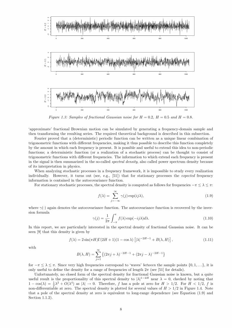
Figure 1.4: The spectral density for H = 0.6, H = 0.7 and H = 0.8.
A low frequency (i.e., small λ) corresponds to a long wavelength. Intuitively, a frequency λ has moreimpact when f(λ) is larger. Thus, the larger H, the larger the low frequency component in the spectraldensity, as seen in Figure 1.4. We recognize this in Figure 1.3, where bigger ‘waves’ are present in the plotfor H = 0.8.
To evaluate the spectral density numerically, the infinite sum in Equation (1.11) must be truncated.When the truncation parameter is chosen quite large, the function evaluation becomes computationally verydemanding. Paxson [47] suggests and tests a useful approximation to overcome this problem. The keyobservation is that
∞∑
j=1
h(j) ≈k∑
j=1
h(j) +1
2
∫ k+1
k
h(x)dx+
∫ ∞
k+1
h(x)dx,
for every increasing integrable function h and k = 0, 1, . . .. With ‘≈’ is meant that the right hand side is areasonable approximation for the left hand side. It is shown [47] that this is already a good approximationfor k = 3. In that case, the approximation becomes
B3(λ,H) =
3∑
j=1
(a+j )−2H−1 + (a−j )−2H−1
+(a+
3 )−2H + (a−3 )−2H + (a+4 )−2H + (a−4 )−2H
8Hπ, (1.12)
where a±j = 2πj ± λ. The author analyzes the relative error of this approximation, and then corrects themean absolute error and linear variation in λ by fitting. As final approximation for B(λ,H), he arrives atB(λ,H)′, where
B(λ,H)′ = (1.0002 − 0.000134λ)
B3(λ,H) − 2−7.65H−7.4
.
Some problems arise when computing a spectral density for fractional Brownian motion, being a non-stationary process: there exists no autocovariance function and Equation (1.9) is thus not applicable. Clearly,a time-independent density (as in the fractional Gaussian noise case) is unsuitable. We will not use thespectral density of fractional Brownian motion in this report, but the interested reader is referred to Flandrin[28] for a discussion.
1.2.3 Another long-range dependent process
Another widely used process with long-range dependence is fractional ARIMA. Since we will encounter thisprocess only sideways, we discuss it briefly. The parameters of this model control the long-range dependenceas well as the short term behavior. The fractional ARIMA model is based on the ARMA model.
An ARMA(p, q) process W = Wk : k = 0, 1, . . . is a short memory process that is the solution of
φ(L)Wk = θ(L)εk,
where φ and θ are polynomials of order p and q respectively and ε is a white noise process, i.e., the εk arei.i.d. standard normal random variables. The lag operator L is defined as LWk = Wk−1.
A generalization of this model is the ARIMA(p, d, q) process for d = 0, 1, . . ., defined by the propertythat (1 − L)dWk is an ARMA(p, q) process. As implied by its name, the fractional ARIMA model admits a
9
fractional value for the parameter d. For this, we have to know how (1 − L)dWk is defined for fractional d.This is formally done by the binomial expansion:
(1 − L)dWk =
∞∑
n=0
(
d
n
)
(−L)nWk,
where the binomial coefficient is defined as(
d
k
)
=Γ(d+ 1)
Γ(d− k + 1)Γ(k + 1).
Since the case d > 1/2 can be reduced to the case −1/2 < d ≤ 1/2 by taking appropriate differences, thelatter case is particularly interesting. W is a stationary process for −1/2 < d < 1/2. Long-range dependenceoccurs for 0 < d < 1/2, implying that the process is also asymptotically second order self-similar in this case.The corresponding Hurst parameter is H = 1/2 + d.
For simulation issues, we refer to [32].
1.3 Implications for network models
Now that it is clear that fractional Brownian motion is a self-similar process with a long-range dependentincremental process (under the restriction H > 1/2), we base a network traffic model on fractional Brownianmotion.
Norros [45] defines fractional Brownian traffic as
A(t) = Mt+√aMBH(t). (1.13)
Here, A(t) represents the number of bits (or data packets) that is offered in the time interval [0, t]. This processhas three parameters M , a and H. M > 0 is interpreted as the mean input rate, a > 0 as a variance coefficient,and 1/2 ≤ H < 1 as the Hurst parameter of de fractional Brownian motion BH . Note that ordinary Browniantraffic (i.e., fractional Brownian traffic with H = 1/2) is a special case, but that no long-range dependence ispresent in the incremental process for H = 1/2.
It may seem a bit surprising that the square root of the mean input rate√M is present in (1.13) as a
scaling factor for the fractional Brownian motion BH(t). Norros motivates this by a superposition property:
the sum A(t) =∑K
i=1A(i)(t) of K independent fractional Brownian traffics with common parameters a and
H but individual mean rates Mi can then be written as A(t) =∑K
i=1Mi +√
a∑K
i=1MiBH(t), where BH is
again a fractional Brownian motion with parameter H.An obvious weakness of this traffic model is that a trajectory of the process may decrease. Since A(t)
represents the cumulative ‘traffic’ in [0, t], the amount of traffic arriving in an interval [t, t+T ] is A(t+T )−A(t),which can be negative. However, this problem is considered of secondary importance. The probability of decayin an interval [t, t + T ] is time-independent and may be quite small, depending on the choice of a and M .To make this more precise, we compute this probability explicitly using the stationarity of the increments offractional Brownian motion and the self-similarity:
P (A(t+ T ) −A(t) < 0) = P (√aM(BH(t+ T ) −BH(t)) +MT < 0)
= P (√aMBH(T ) +MT < 0)
= P (BH(T ) < −√
M/aT )
= P (BH(1) < −√
M/aT 1−H)
= Φ(−√
M/aT 1−H),
where Φ denotes the cumulative distribution function of the standard normal distribution. It is now clearthat this probability rapidly decreases in the interval length T and the factor M/a. This means that negativetraffic is no big issue as long as the timescale (sampling interval) and mean arrival rate (relative to the variancecoefficient) are not too small.
Besides the possibility of negative traffic, the number of bits arriving in a time interval may not be integer-valued. This is also no big problem as long as the number of arrivals in each interval is not too small; potentialfractional values are small compared to this number, which implies that only a small ‘error’ is made. Again,this is a result of the choice of the interval length, the variance coefficient a and arrival rate per time unit M .
10
Norros [44] studies a storage model with fractional Brownian traffic input. The work that is generated bythe traffic process is offered to a server with a fixed capacity of C bits (or data packets) in one time unit. Thework in the system V (t) at time t is called fractional Brownian storage and is defined as
V (t) = sups≤t
(A(t) −A(s) − C(t− s))
for t ≥ 0. Note that this so-called workload process is non-negative, and negative traffic (i.e., a decreasingA) causes no problems for defining the workload process. The following logarithmic asymptotics for the tailbehavior of the distribution of V (t) are obtained:
logP (V (t) > v) ∼ − (C −M)2H
2H2H(1 −H)2−2HaMv2−2H (1.14)
as v → ∞. Thus, the (tail) distribution can be approximated by a Weibull-type distribution. For exactasymptotics of P (V (0) > v), the reader is referred to [35]; see also [50].
For the Brownian case H = 1/2, a = 1 and when C = 1, (1.14) reduces to an exponential tail behavior:1v logP (V (t) > v) ∼ −2(1 −M)/M . As pointed out by the author [44], this coincides with the heavy trafficasymptotics of the M/D/1 system.
This may be illustrated by the fact that fractional Brownian traffic (1.13) with H = 1/2 is (in some sense)the limit of a Poisson process. We will make this precise by studying a Poisson process P = P (t) : t ≥ 0with parameter M . For such a Poisson process,
Q(α)(t) =1√αM
[P (αt) −Mαt]
converges in distribution to a Gaussian variable with variance t as α → ∞. This is a result of the CentralLimit Theorem, the fact that P (αt) =
∑αj=1[P (jt) − P ((j − 1)t)] and the independence of Poisson process
increments. We choose d ≥ 1 time epochs 0 ≤ t1 < . . . < td and set t0 = 0 for notational convenience.
Using the stationarity of the Poisson process, we define Q(α)j = Q(α)(tj) − Q(α)(tj−1) and deduce that Q
(α)j
converges in distribution to a Gaussian random variable with variance tj − tj−1 for j = 1, . . . , d. In addition,(
Q(α)1 , . . . , Q
(α)d
)
has independent elements for fixed α, again by the independence of Poisson process incre-
ments. This independence is asymptotically retained, as can most easily be seen by considering cumulativedistribution functions. For every x1, . . . , xd ∈ R it holds that
F“
Q(α)1 ,...,Q
(α)d
”(x1, . . . , xd) = FQ
(α)1
(x1) · · ·FQ(α)d
(xd)
→ Φt1−t0(x1) · · ·Φtd−td−1(xd) = ΦBM(x1, . . . , xd), (1.15)
where Φσ2(·) denotes the cumulative distribution function of a Gaussian variable with variance σ2. Thelast expression in (1.15) is the cumulative distribution function of the increments of Brownian motion. Weconclude that (P (αt)−αMt)/
√αM converges in finite-dimensional distribution to ordinary Brownian motion.
This suggests the approximation A(t) ≈Mt+√MB(t), which is fractional Brownian traffic with parameters
H = 1/2 and a = 1.Obviously, different techniques (and underlying arrival processes) are required to view fractional Brownian
motion with Hurst parameter H 6= 1/2 as a limiting process. We will briefly come back to this in Chapter 2.
The example of a simple queueing system with fractional Brownian traffic input is very important, becausecompletely different behavior of quantities is observed when a long-range dependent arrival process is modeledinstead of a traditional (e.g., Poisson) process. Much work is done nowadays to address this issue for differentmodels.
For more complicated and realistic systems, simulation becomes an attractive approach. Especially wheninvestigating the tail behavior of random variables (e.g., the number of packets in a buffer), very smallprobabilities have to be simulated. For this, importance sampling or quick simulation (often based on a largedeviation result) may be useful. Fast simulation for long-range dependent processes is a relatively new area,but some work has been done by Huang et al. [33].
1.4 Outline and scientific contribution
As pointed out before, the evaluation of several simulation methods for fractional Brownian motion is themain issue of this report. However, it is often more convenient to work with the (stationary) incremental
11

process of fractional Brownian motion, fractional Gaussian noise (see Section 1.2). Some algorithms to simulatefractional Brownian motion (or fractional Gaussian noise) are described in Chapter 2. The first part addressesthe available exact methods (i.e., the output of the method is a sampled realization of fractional Brownianmotion). Several approximate methods are presented in the second part. A number of methods based onthe so-called Fast Fourier Transformation (FFT) are included in this survey. By the uniform presentation,some insight is gained into the connections between these methods. The Paxson method, which was originallyproposed by Paxson [47] using purely intuitive and asymptotic arguments, thus lacking a real theoreticalfoundation, is shown to fit in a general theoretical framework. This finding does not only clarify manyempirical observations, it also leads to an important improvement of the method. In addition, it is shownthat this FFT-based Paxson method and a generalization of the method, the approximate circulant method,are asymptotically exact in the sense that the variance of the approximation error decays to zero for everysample point as the sample size increases. It also turns out that this approximate circulant method is closelyrelated to an exact method, the Davies and Harte method. From this observation is benefited to study theperformance of this method.
To evaluate approximate simulation methods, we should know if generated approximate samples havethe same properties as exact samples. Statistical estimation and testing techniques that can be used toinvestigate this are discussed in Chapter 3. Although most of the estimation techniques are standard toolsin the analysis of long-range dependent processes, a number of recent estimation methods, based on discretevariations and wavelets, are also reviewed. In addition, a test is proposed that is perfectly suitable for ourevaluation purposes. However, the test is time- and memory-consuming and its power is unknown.
The final chapter, Chapter 4, consists of the actual analysis of the most promising approximate simu-lation methods. First, an error analysis is performed using the insights of Chapter 2. When possible, thecovariance structure of approximate samples is compared to the exact covariance structure. For the so-calledConditionalized Random Midpoint Displacement method, it is described how the covariances of the samplecan numerically be computed. In the original paper, this was only done for the two simplest cases.
Then, the approximate methods are evaluated by an approach that is different from the approaches takenin previous studies. The accuracy of new simulation methods is mostly studied by estimating the Hurstparameter using a number of estimation methods. Note that the Hurst parameter determines the covariancestructure completely, see (1.6). However, these estimation methods are in general based on only one propertyof an exact fractional Gaussian noise sample, thus limiting the conclusive power of the estimates. We canpartially overcome this problem by estimating the Hurst parameter with several estimators. However, we stillcannot be sure that the sample is fractional Gaussian noise when all available estimators produce ‘satisfactory’estimates.
An additional problem is that most estimators are biased. We deal with this in Chapter 4 by usingnonparametric inference techniques.
12
CHAPTER 2
Simulation methods
In the previous chapter, we have seen that the fractional Brownian motion, a Gaussian self-similar process,models some types of data traffic better and more realistically than conventional models. Since few theoret-ical results are known about queueing systems with a fractional Brownian motion-type arrival process, it isimportant to know how this process can be simulated. Therefore, an important role is played by simulationstudies, especially for complex queueing systems. It is the aim of this chapter to describe some simulationmethods for fractional Brownian motion, exact as well as approximate.
Since it is only possible to simulate in discrete time, we adapt a discrete time notation Y0, Y1, . . . for thevalues of the fractional Brownian motion at the discrete time epochs 0, 1, . . .. Once this fractional Brownianmotion sample is simulated, a realization on another equispaced grid is obtained by using the self-similarityproperty.
2.1 Exact methods
2.1.1 The Hosking method
The Hosking method (also known as the Durbin or Levinson method) is an algorithm to simulate a generalstationary Gaussian process; therefore, we will focus on the simulation of fractional Gaussian noise X0, X1, . . ..Recall that a fractional Brownian motion sample Y0, Y1, . . . is obtained from a fractional Gaussian noise sampleby taking cumulative sums. The method generates Xn+1 given Xn, . . . , X0 recursively. It does not use specificproperties of fractional Brownian motion nor fractional Gaussian noise; the algorithm can be applied to anystationary Gaussian process. The key observation is that the distribution of Xn+1 given the past can explicitlybe computed.
Write γ(·) for the covariance function of the (zero-mean) process, that is
γ(k) := EXnXn+k,
for n, k = 0, 1, 2, . . .. Assume for convenience that γ(0) = 1. Furthermore, let Γ(n) = (γ(i − j))i,j=0,...,n bethe covariance matrix and c(n) be the (n + 1)–column vector with elements c(n)k = γ(k + 1), k = 0, . . . , n.Define the (n + 1) × (n + 1) matrix F (n) = (1(i = n − j))i,j=0,...,n, where 1 denotes the indicator function.Note that premultiplying this matrix with a column vector or postmultiplying with a row vector ‘flips’ thisvector.
The matrix Γ(n+ 1) can be splitted as follows:
Γ(n+ 1) =
(
1 c(n)′
c(n) Γ(n)
)
(2.1)
=
(
Γ(n) F (n)c(n)c(n)′F (n) 1
)
, (2.2)
where the prime denotes vector transpose.We next compute the conditional distribution of Xn+1 given Xn, . . . , X0. In fact, we show that this
distribution is Gaussian with expectation µn and variance σ2n given by
µn := c(n)′Γ(n)−1
Xn
...X1
X0
, σ2n := 1 − c(n)′Γ(n)−1c(n). (2.3)
13
Define d(n) = Γ(n)−1c(n) for convenience. It is left to the reader to check with (2.1) and (2.2) that thefollowing two expressions for the inverse of Γ(n+ 1) hold:
Γ(n+ 1)−1 =1
σ2n
(
1 −d(n)′
−d(n) σ2nΓ(n)−1 + d(n)d(n)′
)
(2.4)
=1
σ2n
(
σ2nΓ(n)−1 + F (n)d(n)d(n)′F (n) −F (n)d(n)
−d(n)′F (n) 1
)
, (2.5)
From (2.4) is readily deduced that for each x ∈ Rn+1 and y ∈ R:
(
y x′)
Γ(n+ 1)−1
(
yx
)
=(y − d(n)′x)2
σ2n
+ x′Γ(n)−1x. (2.6)
This implies that the distribution of Xn+1 given Xn, . . . , X0 is indeed Gaussian with expectation µn andvariance σ2
n.Now that we know this distribution, the required sample is found by generating a standard normal random
variable X0 and simulate Xn+1 recursively for n = 0, 1, . . .. Of course, the difficulty is to organize thecalculations to avoid matrix inversion in each step. The algorithm proposed by Hosking [32] computes d(n)recursively. The algorithm is presented here in a slightly different but faster way than in the original article.
Suppose we know µn, σ2n and τn := d(n)′F (n)c(n) = c(n)′F (n)d(n). Using (2.5), it is easy to see that σ2
n
satisfies the recursion
σ2n+1 = σ2
n − (γ(n+ 2) − τn)2
σ2n
.
A recursion for d(n+ 1) = Γ(n+ 1)−1c(n+ 1) is also obtained from (2.5):
d(n+ 1) =
(
d(n) − φnF (n)d(n)φn
)
,
with
φn =γ(n+ 2) − τn
σ2n
.
The first n elements of the (n+2)–row vector d(n+1) can thus be computed from d(n) and φn. Given d(n+1),it is clear how to compute µn+1, σ
2n+1 and τn+1. We start the recursion with µ0 = γ(1)X0, σ
20 = 1 − γ(1)2
and τ0 = γ(1)2. Note that cumulative sums have to be computed when a sample fractional Brownian motionY0, Y1, . . . is required.
An approach that is closely related to the Hosking algorithm is the innovations algorithm. Instead ofrecursively generating Xn+1 given Xn, . . . , X0, this method simulates the innovation Xn+1 − µn given Xn −µn−1, . . . , X1 − µ0, X0. An advantage of this algorithm is that it can also be applied to non-stationaryprocesses. For details we refer to [11].
Because of the computations in the recursions of d(n), µn and τn, the algorithm’s complexity is of orderN2 for a sample of size N . As an example, the computation of d(n) − φnF (n)d(n) for given φn and d(n)requires order n computer flops. Doing this for n = 1, 2, . . . , N requires order N 2 flops.
An advantage of the Hosking method is that traces can be generated on-the-fly. This means that thesample size does not need to be known in advance. This occurs for example when a simulation should stopat some random time.
Another strength of this method is its extreme simplicity. This is used in Huang et al. [33] to expresssome likelihoods in terms of by-products of the algorithm, like φn. Based on these likelihoods, an algorithmfor fast simulation in a queueing framework is given.
When more than one trace is needed, as in simulation studies with more than one run, most of thecomputations need not be done again. However, because the calculation of µn depends on the generatedpoints X0, . . . , Xn, the number of computer flops is still of order N 2; the time complexity is thus not reduced.
2.1.2 The Cholesky method
Not surprisingly, the Cholesky method (e.g., [4]) makes use of the so-called Cholesky decomposition of thecovariance matrix. This means that the covariance matrix Γ(n) can be written as L(n)L(n)′, where L(n) isan (n+ 1)× (n+ 1) lower triangular matrix. Denoting element (i, j) of L(n) by lij for i, j = 0, . . . , n, L(n) issaid to be lower triangular if lij = 0 for j > i. It can be proven that such a decomposition exists when Γ(n)is a symmetric positive definite matrix.
14
Unlike the Hosking method, the Cholesky method can be applied to non-stationary Gaussian processes,but we assume stationarity for notational reasons.
The elements of L(n) can be computed by noting that element (i, j) of L(n)L(n)′ and Γ(n) should beequal for j ≤ i (then also for j > i because of the symmetry). That is,
γ(i− j) =
j∑
k=0
likljk, j ≤ i. (2.7)
This equation reduces to γ(0) = l200 for i = j = 0. For i = 1 we get the two equations
γ(1) = l10l00, γ(0) = l210 + l211
determining l10 and l11. Since it is clear from this that lij cannot depend on n, L(n + 1) can be computedfrom L(n) by adding a row (and some zeros to make L(n+ 1) lower triangular) determined by
ln+1,0 =γ(n+ 1)
l00
ln+1,j =1
ljj
(
γ(n+ 1 − j) −j−1∑
k=0
ln+1,kljk
)
, 0 < j ≤ n
l2n+1,n+1 = γ(0) −n∑
k=0
l2n+1,k.
From these formulas follows that L(n) is unique under the additional restriction that the elements on themain diagonal are strictly positive. When Γ(n+1) is a positive definite matrix, the non-negativity of l2n+1,n+1
is guaranteed, so that the matrix L(n+ 1) is real.Denote by V (n) = (Vi)i=0,...,n an (n + 1)–column vector of i.i.d. standard normal random variables, and
construct V (n + 1) from V (n) by padding a standard normal random variable. The key idea is to simulateX(n) = L(n)V (n) recursively. For every n ≥ 0, X(n) has zero mean and covariance matrix
Cov(L(n)V (n)) = L(n)Cov(V (n))L(n)′ = L(n)L(n)′ = Γ(n).
Summarizing, Xn+1 can quite easily be simulated once L(n+ 1) is computed:
Xn+1 =n+1∑
k=0
ln+1,kVk. (2.8)
Like the Hosking method, one does not need to set the time horizon in advance. The drawback of themethod is that it becomes slow (order N 3 for N points) and demanding in terms of storage, because thematrix L(n), that grows in every step of the recursion, has to be kept in memory.
When more than one sample is needed, a lot of computing time can be saved by calculating L(n) onlyonce. In fact, every additional sample then requires order N 2 computer flops.
Although not obvious by comparing the algorithms, the Hosking method is essentially equivalent to theCholesky method (but faster!) in the sense that the Hosking method computes implicitly the same matrixL(n). Indeed, in the Hosking method, Xn+1 is generated by µn +σnVn+1 and µn only depends on Xn, . . . , X0.Analogously, Xn is generated by µn−1 + σn−1Vn, where µn−1 only depends on Xn−1, . . . , X0. Repeating this,Xn+1 is generated by some linear combination of n+ 1 i.i.d. standard normal random variables:
Xn+1 =
n+1∑
k=0
hn+1,kVk,
where we know that hn+1,n+1 = σn > 0. The analogy with (2.8) is now clear: just like the Cholesky method,the sample is generated by multiplying a vector with i.i.d. standard normal components with a square lowertriangular matrix. But the matrices must then be equal, as the Cholesky decomposition is unique if theelements on the main diagonal are positive!
2.1.3 The Davies and Harte method
This algorithm was originally proposed by Davies and Harte [19] and was later simultaneously generalized byDietrich and Newsam [23] and Wood and Chan [59]. Like the Hosking and the Cholesky method, the method
15
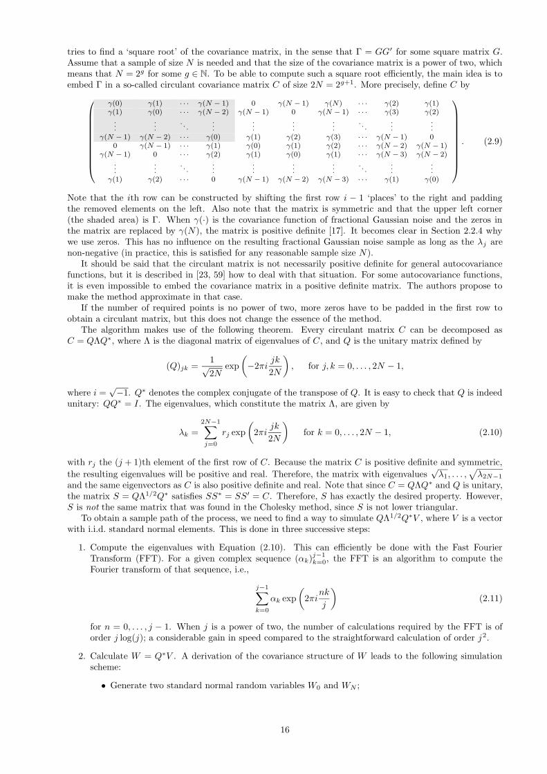
tries to find a ‘square root’ of the covariance matrix, in the sense that Γ = GG′ for some square matrix G.Assume that a sample of size N is needed and that the size of the covariance matrix is a power of two, whichmeans that N = 2g for some g ∈ N. To be able to compute such a square root efficiently, the main idea is toembed Γ in a so-called circulant covariance matrix C of size 2N = 2g+1. More precisely, define C by
γ(0) γ(1) · · · γ(N − 1) 0 γ(N − 1) γ(N) · · · γ(2) γ(1)γ(1) γ(0) · · · γ(N − 2) γ(N − 1) 0 γ(N − 1) · · · γ(3) γ(2)
.
.....
. . ....
.
.....
.
... . .
.
.....
γ(N − 1) γ(N − 2) · · · γ(0) γ(1) γ(2) γ(3) · · · γ(N − 1) 00 γ(N − 1) · · · γ(1) γ(0) γ(1) γ(2) · · · γ(N − 2) γ(N − 1)
γ(N − 1) 0 · · · γ(2) γ(1) γ(0) γ(1) · · · γ(N − 3) γ(N − 2)...
..
.. . .
..
....
..
....
. . ....
..
.γ(1) γ(2) · · · 0 γ(N − 1) γ(N − 2) γ(N − 3) · · · γ(1) γ(0)
. (2.9)
Note that the ith row can be constructed by shifting the first row i − 1 ‘places’ to the right and paddingthe removed elements on the left. Also note that the matrix is symmetric and that the upper left corner(the shaded area) is Γ. When γ(·) is the covariance function of fractional Gaussian noise and the zeros inthe matrix are replaced by γ(N), the matrix is positive definite [17]. It becomes clear in Section 2.2.4 whywe use zeros. This has no influence on the resulting fractional Gaussian noise sample as long as the λj arenon-negative (in practice, this is satisfied for any reasonable sample size N).
It should be said that the circulant matrix is not necessarily positive definite for general autocovariancefunctions, but it is described in [23, 59] how to deal with that situation. For some autocovariance functions,it is even impossible to embed the covariance matrix in a positive definite matrix. The authors propose tomake the method approximate in that case.
If the number of required points is no power of two, more zeros have to be padded in the first row toobtain a circulant matrix, but this does not change the essence of the method.
The algorithm makes use of the following theorem. Every circulant matrix C can be decomposed asC = QΛQ∗, where Λ is the diagonal matrix of eigenvalues of C, and Q is the unitary matrix defined by
(Q)jk =1√2N
exp
(
−2πijk
2N
)
, for j, k = 0, . . . , 2N − 1,
where i =√−1. Q∗ denotes the complex conjugate of the transpose of Q. It is easy to check that Q is indeed
unitary: QQ∗ = I. The eigenvalues, which constitute the matrix Λ, are given by
λk =
2N−1∑
j=0
rj exp
(
2πijk
2N
)
for k = 0, . . . , 2N − 1, (2.10)
with rj the (j + 1)th element of the first row of C. Because the matrix C is positive definite and symmetric,
the resulting eigenvalues will be positive and real. Therefore, the matrix with eigenvalues√λ1, . . . ,
√
λ2N−1
and the same eigenvectors as C is also positive definite and real. Note that since C = QΛQ∗ and Q is unitary,the matrix S = QΛ1/2Q∗ satisfies SS∗ = SS′ = C. Therefore, S has exactly the desired property. However,S is not the same matrix that was found in the Cholesky method, since S is not lower triangular.
To obtain a sample path of the process, we need to find a way to simulate QΛ1/2Q∗V , where V is a vectorwith i.i.d. standard normal elements. This is done in three successive steps:
1. Compute the eigenvalues with Equation (2.10). This can efficiently be done with the Fast FourierTransform (FFT). For a given complex sequence (αk)j−1
k=0, the FFT is an algorithm to compute theFourier transform of that sequence, i.e.,
j−1∑
k=0
αk exp
(
2πink
j
)
(2.11)
for n = 0, . . . , j − 1. When j is a power of two, the number of calculations required by the FFT is oforder j log(j); a considerable gain in speed compared to the straightforward calculation of order j2.
2. Calculate W = Q∗V . A derivation of the covariance structure of W leads to the following simulationscheme:
• Generate two standard normal random variables W0 and WN ;
16
• For 1 ≤ j < N , generate two independent standard normal random variables V(1)j and V
(2)j and let
Wj =1√2(V
(1)j + iV
(2)j )
W2N−j =1√2(V
(1)j − iV
(2)j ).
The resulting vector W has the same distribution as Q∗V .
3. Compute Z = QΛ1/2W :
Zk =1√2N
2N−1∑
j=0
√
λjWj exp
(
−2iπjk
2N
)
. (2.12)
Again, this calculation is best done with the Fast Fourier Transform for maximum speed. In summary,the sequence (Zk)2N−1
k=0 is the Fourier transform of
wk :=
√
λk
2N V(1)k k = 0;
√
λk
4N
(
V(1)k + iV
(2)k
)
k = 1, . . . , N − 1;√
λk
2N V(1)k k = N ;
√
λk
4N
(
V(1)2N−k − iV
(2)2N−k
)
k = N + 1, . . . , 2N − 1,
(2.13)
A sample of fractional Gaussian noise is obtained by taking the first N elements of Z. It is left to thereader to check that Z is real by construction.
Looking at (2.9), we see that the last N elements of Z also have the desired covariance structure. So in thissetup, we get a second sample ‘for free’. However, these two samples may not be put together to obtain adouble-sized sample, because the correlation structure between the two samples is not according to fractionalGaussian noise. Since the two samples are moreover not independent, this second sample is mostly useless.
The main advantage of this method is the speed. More precisely, the number of computations is of orderN log(N) for N sample points. When more traces are needed, the eigenvalues need only to be calculated once.However, the calculations in the second step should be done separately for each trace. Because of this, thenumber of computations is still of order N log(N).
2.2 Approximate methods
2.2.1 Stochastic representation method
As we saw in Section 1.2.1, Mandelbrot and van Ness [42] defined fractional Brownian motion by a stochasticintegral with respect to ordinary Brownian motion. A natural idea is to approximate this integral by Riemann-type sums to simulate the process.
When approximating (1.3) by sums, the first integral should be truncated, say at −b. The approximationBH(n) is for n = 1, . . . , N given by
BH(n) = CH
(
0∑
k=−b
[(n− k)H−1/2 − (−k)H−1/2]B1(k) +
n∑
k=0
(n− k)H−1/2B2(k)
)
, (2.14)
where B1 resp. B2 are vectors of b+1 resp. N+1 i.i.d. standard normal variables, mutually independent. Theconstant CH in (2.14) is not equal to the constant in (1.3), since we switched to study normalized fractionalBrownian motion.
The approximation can be made better by increasing the truncation parameter b and choosing a finer gridfor the Riemann sums. In [14], it is suggested to choose b = N 3/2. This method is only interesting from ahistorical point of view and is considered no good way to generate fractional Brownian motion.
2.2.2 Aggregating packet processes
A possible explanation for the self-similarity in LAN traffic is the presence of the Noah effect in the packetprocesses of individual source-destination pairs, cf. Section 1.1.1. We can therefore simulate processes on themicro-scale and aggregate them to obtain Brownian traffic.
17
For this, we first have to gain more insight into this aggregation result. This section is mainly based onWillinger et al. [58].
Suppose there are S i.i.d. sources. Each source s has active and inactive periods, which is modeled bya stationary binary time series W (s)(t) : t ≥ 0. W (s)(t) = 1 means that the source is sending a packetat time t and this is not the case if W (s)(t) = 0. The lengths of the active (‘ON’) periods are i.i.d., thoseof the inactive periods (‘OFF’) are i.i.d., and the lengths of the ON- and OFF-periods are independent. AnOFF-period follows an ON-period and the ON- and OFF-period lengths may have different distributions.Rescaling time by a factor T , let
WS(Tt) =
∫ Tt
0
(
S∑
s=1
W (s)(u)
)
du,
be the aggregated cumulative packet counts in the interval [0, T t].For simplicity, let the distributions of the ON- and OFF-periods both be Pareto with joint parameter
1 < α < 2. Recall that a random variableX has a Pareto distribution with parameter α > 0 if P (X > t) = t−α
for t ≥ 1. Note that the ON- and OFF-periods have infinite variance as a result of 1 < α < 2.It is pointed out in [58] that the following limit result holds for WS(Tt) : 0 ≤ t <∞:
limT→∞
limS→∞
T−HS−1/2
(
WS(Tt) − 1
2TSt
)
= σBH(t) (2.15)
for some σ > 0, where H = (3 − α)/2 and BH(t) denotes fractional Brownian motion with Hurst parameterH. The limits are limits in the sense of finite-dimensional distributions. A similar result holds when otherkinds of heavy-tailed distributions for the ON- and OFF-periods are chosen.
We should interpret this asymptotic result with care, because (2.15) is not valid when the order of thelimits is reversed. Forgetting about this, we can intuitively say that WS(Tt) closely resembles
1
2TSt+ TH
√SσBH(t),
which is fractional Brownian traffic with parameters M = 12TS and a = 2σ2T 2H−1 in the notation of Section
1.3.The above result can be used for simulation purposes, by aggregating a large number of sources with Pareto
ON- and OFF-periods. This results in an order N algorithm when N sample points are needed. However, thenumber of sources that have to be aggregated to get proper output may be quite large, which may result ina serious slowdown. Moreover, there is no clue how many sources are required to produce reasonable results.In fact, because of the mentioned problem with the reversal of the limits, we have to be very suspicious aboutthe obtained sample.
Another aggregation method for simulating long-range dependent processes uses the M/G/∞ queueingmodel, where customers arrive according to a Poisson process and have service times drawn from a distributionwith infinite variance. When Xt denotes the number of customers in the system at time t, Xt : t ≥ 0 isasymptotically self-similar [40]. Again, one must trade off length of computation for degree of self-similarity.
2.2.3 (Conditionalized) Random Midpoint Displacement
The Hosking and Cholesky method generate a fractional Gaussian noise sample recursively. Instead of sim-ulating Xn+1 given the whole past, the generation may be sped up by simulating Xn+1 given the last mgenerated values for some m ≥ 1. However, the long-term correlations are then destroyed, which makes thisapproach not suitable for generating long-range dependent processes.
The idea behind the Random Midpoint Displacement (RMD) method is to generate the Xn in anotherorder, so that conditioning on only one already generated sample point preserves some long-range dependence.The suitability of the RMD method in a teletraffic framework was first investigated in [39].
A generalization of the RMD method, the Conditionalized RMD method [46], generates the sample in thesame order as the RMD method, but more sample points are used in the conditioning. The method has twointeger-valued truncation parameters, l ≥ 0 and r ≥ 1. We construct a sample of fractional Brownian motionon [0, 1] for notational reasons. Note that this sample can be scaled onto an interval of any desired lengthusing the self-similarity property.
Denote Xij = BH(j2−i) − BH((j − 1)2−i) for i = 0, 1, 2, . . ., j = 1, . . . , 2i. For fixed i, Xi = Xij : j =1, . . . , 2i can be considered a scaled sample of fractional Gaussian noise of size 2i. However, there is a strongcorrelation between these samples for different i:
Xi−1,j = Xi,2j +Xi,2j+1. (2.16)
18
The Conditionalized RMD algorithm makes use of this recursive structure by simulating the processesX0,X1, . . . until the desired resolution, say N = 2g, is reached. A fractional Brownian motion sample isthen found by taking cumulative sums of Xg. We will refer to the Conditionalized RMD method with trun-cation parameters l and r as RMDl,r.
Assume that we have obtained realizations of X0,X1, . . . ,Xi−1. To obtain a realization of Xi as well, itsuffices to generate Xi,j for odd j because of (2.16). Note that the realization of Xi−1 contains all generatedinformation so far. Let us proceed from left to right, and assume that Xi1, . . . , Xi,2k have been generated(k = 0, 1, . . . , 2i−1−1). When we continue to generateXi,2k+1 by conditioning on all past values Xi1, . . . , Xi,2k
in Xi and all values of Xi−1 that are still relevant, Xi−1,k+1, . . . , Xi−1,2i−1 , no approximation is involved. Thealgorithm stays then exact but also becomes very slow. Therefore, Norros et al. [46] propose to use only thelast l values of Xi1, . . . , Xi,2k (if possible) and the first r values of Xi−1,k+1, . . . , Xi−1,2i−1 (if possible). Forl = 0 and r = 1, the algorithm reduces to the original RMD method described in [39].
Putting this mathematically, we set
Xi,2k+1 = e(i, k)(
Xi,(2k−l+1)∨1, . . . , Xi,2k, Xi−1,k+1, . . . , Xi−1,(k+r)∧2i−1
)′+√
v(i, k)Uik,
where Uik : i = 0, 1, . . . ; k = 0, . . . , 2i−1 − 1 is a set of independent standard Gaussian variables, e(i, k) is arow vector such that
e(i, k)(
Xi,(2k−l+1)∨1, . . . , Xi,2k, Xi−1,k+1, . . . , Xi−1,(k+r)∧2i−1
)′
= E[
Xi,2k+1|Xi,(2k−l+1)∨1, . . . , Xi,2k, Xi−1,k+1, . . . , Xi−1,(k+r)∧2i−1
]
,
and v(i, k) is the scalar given by
Var[
Xi,2k+1|Xi,(2k−l+1)∨1, . . . , Xi,2k, Xi−1,k+1, . . . , Xi−1,(k+r)∧2i−1
]
,
following the convention a∨b = max(a, b) and a∧b = min(a, b). The quantities e(i, k) and v(i, k) are computedwith a slight modification of the technique that was used in the derivation of the Hosking algorithm, Equation(2.6). The covariances that are needed for this are computed by straightforward substituting the definition ofXij and applying (1.6).
By the stationarity of the increments of BH and by self-similarity, e(i, k) is independent of i and kwhen 2k ≥ l and k ≤ 2i−1 − r. Moreover, it does not depend on l and r when 2i < l + 2r. Thus, thenumber of vectors e(i, k) that needs to be known up to stage j, where j is the smallest integer greaterthan log2(l + 2r), is the total number of vectors that should be computed. This number is not larger than1 + 2 + 22 + . . .+ 2j−1 = 2j − 1 < 2l + 4r. The same holds for the scalars v(i, k), except that ‘independencewith respect to i’ is replaced by scaling a constant factor 2−2Hi.
Some optimizing may be done to calculate the needed vectors e(i, k) and scalars v(i, k) (e.g., in a recursiveapproach like Hosking’s method rather than explicit matrix inversion), but since 2l + 4r is typically quitesmall and since the sizes of the matrices are therefore also quite small, not much computational gain shouldbe expected from this (if at all).
It is clear that the algorithm as described above is unsuitable for on-the-fly generation of the sample,because the time horizon should be known in advance. It is, however, not necessary to generate the splits inexactly the same order as above. That is, instead of generating each resolution completely before moving tothe finer one, we can have several unfinished resolutions at the same time. For details we refer to [46].
The complexity of this algorithm is of order N when a sample of size N is needed. Note that this is fasterthan the fastest exact method. Therefore, the conditionalized RMD algorithm is extremely interesting forsimulation purposes. In Chapter 4, we compare the output this method for several values of l and r to see ifa reasonable trade-off between speed and precision is made.
2.2.4 Spectral simulation, the Paxson method and the approximate circulantmethod
Spectral simulation is a method to simulate stationary Gaussian processes using spectral analysis. Whenextracting an algorithm out of spectral considerations, the Fast Fourier Transform (FFT) plays a major role.
First, we describe the general principle of spectral simulation, which was already briefly touched in Section1.2.2. The idea of spectral simulation is to simulate a process in the frequency domain and transform theresulting series to the time domain. Although it is not possible to obtain an exact fractional Brownian motionsample when this approach is followed, we will shortly see that the accuracy increases as the sample sizegrows.
In the course of the exposition, it becomes clear that spectral simulation is closely related to the Paxsonmethod and the Davies and Harte method. The resulting modification of the Davies and Harte method(making the exact algorithm approximate to speed up the simulation) will be called the approximate circulantmethod.
19
Spectral simulation
We have already seen that unambiguous spectral analysis of stochastic processes is only possible for stationaryprocesses. Throughout this subsection, we assume that the required sample size N is a power of two. We dealwith a general real-valued stationary Gaussian process with spectral density f(λ), possibly with a singularityat 0 (as in the case of fractional Gaussian noise, on which we will focus). See Section 1.2.2 for a review ofspectral densities. The considerations in this subsection are mainly based on the theory of spectral analysis,see, e.g., [41, 51]. The results of this subsection have been published as [22].
The spectral analysis of a stationary discrete-time Gaussian process X = Xn : n = 0, . . . , N − 1 showsthat it can be represented in terms of the spectral density as
Xn =
∫ π
0
√
f(λ)
πcos(nλ)dB1(λ) −
∫ π
0
√
f(λ)
πsin(nλ)dB2(λ), (2.17)
where the equality is to be understood as equality in distribution. This result is called the spectral theorem.The two integrators are mutually independent (ordinary) Brownian motions; for the definition of such astochastic integral, see Section 1.2.1. Using elementary stochastic calculus and (1.10), its validity is easilychecked by showing that the right-hand side of (2.17) has covariance function (1.7).
Spectral simulation is based on approximating Equation (2.17); the integrand is replaced by a simplefunction. Define ξn(λ) :=
√
f(λ)/π cos(nλ) and fix some integer `. After setting tk = πk/` for k = 0, . . . , `−1,
we define a simple function ξ(`)n on [0, π] for 0 ≤ n ≤ N − 1 by
ξ(`)n (λ) :=
√
f(t1)
πcos(nt1)10(λ) +
`−1∑
k=0
√
f(tk+1)
πcos(ntk+1)1(tk,tk+1](λ). (2.18)
Let θ(`)n (λ) be defined as ξ
(`)n (λ), but with the cosine terms replaced by sine terms. The first integral in
(2.17) is approximated by∫ π
0ξ(`)n (λ)dB1(λ), which can be computed using Equation (1.4). Since a similar
approximation can be made for the second integral, we arrive at the following approximation X(`)n of Xn:
X(`)n :=
`−1∑
k=0
√
f(tk+1)
`
[
cos(ntk+1)U(0)k − sin(ntk+1)U
(1)k
]
, (2.19)
where U(i)k are again i.i.d. standard normal random variables for k = 0, . . . , ` − 1. The two vectors U (0) and
U (1) should also be mutually independent, since B1 and B2 are independent as well.It should be noted that for H > 1/2, we approximate the spectral density by functions that have no
pole at 0. As already pointed out, this pole is equivalent to long-range dependence. Hence, we approximatea long-range dependent process by a short-range dependent process. Still, we may obtain a sample with acovariance structure that approximates the structure determined by (1.7) and (1.8) very well. This issue isexplored further in Section 4.2.
The FFT can be used to calculate (2.19) efficiently. To this end, we define the sequence (ak)k=0,...,2`−1 by
ak :=
0 k = 0;12
(
U(0)k−1 + iU
(1)k−1
)
√
f(tk)/` k = 1, . . . , `− 1;
U(0)k−1
√
f(tk)/` k = `;12
(
U(0)2`−k−1 − iU
(1)2`−k−1
)
√
f(t2`−k)/` k = `+ 1, . . . , 2`− 1.
(2.20)
Using (2.11), one can check that the Fourier transform of (ak) is real and equals (2.19).
Since ξ(`)n approximates ξn better for larger `, an interesting question is whether the approximate sample
converges to an exact sample as ` → ∞. However, different types of convergence of random variables andprocesses exist; it is at first sight not clear in what sense the approximate sample converges. In the remainderof this subsection, we deal with this convergence issue.
Convergence
We start by deriving the covariance structure of X(`). From (2.19) it follows that the covariance between X(`)m
and X(`)n for n,m = 0, . . . , N − 1 is given by
Cov(X(`)m , X(`)
n ) =
`−1∑
k=0
f(tk+1)
`cos((m− n)tk+1), (2.21)
20
which depends only on m − n. Hence, the spectral simulation method produces stationary approximatesamples. Moreover, the covariances approach their exact values as `→ ∞:
`−1∑
k=0
f(tk+1)
`cos(ntk+1) → 2
∫ π
0
f(λ)
2πcos(nλ)dλ =
1
2π
∫ π
−π
f(λ) exp(−inλ)dλ = γ(n), (2.22)
where the last equality is (1.10). A more detailed numerical analysis of the covariance structure is deferredto Chapter 4.
It is readily checked with (1.10) that Cov(X(`)m , X
(`)n ) converges to γ(|m − n|) as ` → ∞. From this fact,
it is not difficult to deduce that the finite-dimensional distributions of X(`) converge in distribution to thecorresponding finite-dimensional distributions of X as ` → ∞. However, we will not prove this, since we can
prove an even stronger convergence result: every sample point X(`)n converges in L2–norm to the corresponding
exact sample point Xn as `→ ∞.The proof of this fact is based on the definition of the stochastic integral appearing in (2.17). Because f
is integrable, the function ξn is certainly square integrable for 0 ≤ n ≤ N − 1. Recall that the discussion on
stochastic integration showed that if the sequence of simple functions (ξ(`)n )` satisfies, for fixed 0 ≤ n ≤ N −1,
lim`→∞
∫ π
0
[
ξn(λ) − ξ(`)n (λ)]2
dλ = 0, (2.23)
then∫ π
0ξ(`)n (λ)dB1(λ) converges in L2–norm to
∫ π
0ξn(λ)dB1(λ) as `→ ∞. It is indeed true that (2.23) holds;
a similar result holds for the second integrand of (2.17). A proof of these facts can be found in the appendix
of this chapter. By the independence of B1 and B2, we deduce that every sample point X(`)n converges to Xn
in L2–norm, i.e., in mean square sense.
Since the ‘error’ X(`)n −Xn is a centered Gaussian variable for every n (with a variance that decays to zero
in `), we have
E|X(`)n −Xn|p =
Γ((p+ 1)/2)√π
[
2E|X(`)n −Xn|2
]p/2
. (2.24)
Thus, X(`)n converges to Xn in Lp–norm for every p ≥ 1! Because of the normality, this is equivalent to
convergence in probability. This convergence of the individual sample points is readily extended to a jointconvergence result: the finite-dimensional distributions of X(`) converge in probability to the correspondingfinite-dimensional distributions of X as `→ ∞.
An interesting question is at what rate the convergence takes place. By the way the stochastic integralis constructed, this rate is related to the rate of convergence of (2.23) and its θn-counterpart. Let ε > 0 bearbitrary, and suppose that H > 1/2. As
√
f(λ)/(2π) cos(nλ) behaves like C|λ|1−2H near λ = 0, one has on[0, π/`], for large `,
(C − ε)λ1/2−H ≤√
f(λ)
2πcos(nλ) ≤ (C + ε)λ1/2−H .
Set C ′ := [(C + ε)/(C − ε)]1/(1/2−H) < 1, then
σ2
X(`)n −Xn
= ‖ξn − ξ(`)n ‖2 + ‖θn − θ(`)n ‖2
≥∫ π/`
0
(√
f(λ)
2πcos(nλ) −
√
f(π/`)
2πcos(nπ/`)
)2
dλ
≥∫ C′π/`
0
(
(C − ε)λ1/2−H − (C − ε)(C ′π/`)1/2−H)2
dλ
∼ K`2H−2,
where K denotes some constant. Thus, the rate of convergence is quite slow.Since the length of the output sequence of the FFT algorithm applied to (2.20) must be at least the sample
size N , the smallest possible choice for ` is N/2, although better results are obtained for larger `. For ` = N/2,the spectral simulation approach is closely related to the Paxson method, as will now be made clear.
The Paxson method
Paxson [47] proposes a rather intuitive method for simulating fractional Gaussian noise. By studying theoutput statistically, he tests if the resulting samples have indeed the desired properties. Unfortunately, the
21
paper lacks a thorough justification of the proposed procedure, and it remains unclear why the obtainedsample should be (close to) Gaussian.
However, with the formulas above, it is possible to make the arguments precise. In the Paxson method,the approximate fGn sample is the Fourier transform of
bk :=
0 k = 0;√
Rkf(tk)N exp(iΦk) k = 1, . . . , N/2;
b∗N−k k = N/2 + 1, . . . , N − 1,
where Rk are independent exponentially distributed random variables with mean 1 for k ≥ 1, and the as-terisk denotes the complex conjugate. Besides ΦN/2, which is set to zero, the Φk are independent uniformlydistributed random variables on [0, 2π] for k ≥ 1, also independent of the Rk. In this case, tk equals 2πk/N .Note that the obtained sample is real by construction.
Because Rk is exponentially distributed with mean 1,√
2Rk exp(iΦk) has the same distribution as U(0)k +
iU(1)k , where U
(0)k and U
(1)k are independent standard normal random variables in the usual notation. This
fact is also used in the well-known Box-Muller algorithm to simulate Gaussian random variables (e.g., [4]).Let us now compare this with the spectral simulation method for ` = N/2. In that case, the sample is the
Fourier transform of (see (2.20))
b′k :=
0 k = 0;√
f(tk)2N
(
U(0)k−1 + iU
(1)k−1
)
k = 1, . . . , N/2 − 1;√
2f(tk)N U
(0)k−1 k = N/2;
√
f(tk)2N
(
U(0)N−k−1 − iU
(1)N−k−1
)
k = N/2 + 1, . . . , N − 1,
(2.25)
where the U(i)k have their usual meaning. At this point it becomes clear what the relation is between the
spectral method and the Paxson method; by comparing bk to b′k, we see that the value of bN/2 is the only
difference (of course, the indexing of the random variables U (i) differs, but this has no impact). However,this effect will vanish for ‘large’ N ; it is readily checked that it does not affect the convergence result of theprevious subsection. Thus, the accuracy of the Paxson method increases with the sample size N , and is evenexact as N → ∞ in the sense that each sample point converges to an ‘exact’ sample point in probability.
We can now argue that Paxson’s suggestion to set ΦN/2 = 0 is not useful, since this destroys the normalityof bN/2, which is reflected in every sample point, cf. (2.11). This is the reason that Paxson finds in some casesthat the resulting sample points have a ‘nearly’ normal distribution. Therefore, we set
bN/2 =
√
f(tN/2)
2NU
(0)N/2,
although (as before) the imaginary part has no influence on the sample. In the remaining of this paper, wecall this improved Paxson method simply the Paxson method.
The method is faster than the Davies and Harte method, although still of order N log(N). This is becausethe Paxson method requires just one Fourier transform of a sequence of size N , instead of two transformsof size 2N . Hence, the Paxson method is approximately four times faster than the exact Davies and Hartemethod, provided N is large. It may thus offer a good alternative to exact simulation when large sample sizesare required. A more detailed runtime comparison is made in Chapter 4.
The fBm samples produced with Paxson fGn samples have the special property that the end point isalways 0. This property is easily seen by using the definition of the FFT transform (2.11):
N−1∑
n=0
N−1∑
k=0
bk exp
(
2πink
N
)
=
N−1∑
k=0
bk
N−1∑
n=0
exp
(
2πink
N
)
= Nb0 = 0.
This highly undesirable property of Paxson fBm samples can be regarded as a fractional Brownian bridge-effect.
Having recognized that the Paxson method equals the spectral simulation method with ` = N/2, a naturalquestion is what can be said about spectral simulation with ` = N . The next subsection shows that there isa connection with the Davies and Harte method.
The approximate circulant method; connection with the Davies and Harte method
We now make the observation that the spectral simulation approach is related to the circulant diagonalizationalgorithm of Davies and Harte. In that algorithm, the λk are calculated with (2.11), which can be rewritten
22
as
λk =N−1∑
j=0
γ(j) exp
(
2πijk
2N
)
+N−1∑
j=1
γ(j) exp
(
2πi(2N − j)k
2N
)
=N−1∑
j=−N+1
γ(j) exp
(
2πijk
2N
)
. (2.26)
Letting tk = πk/N , this can be approximated by the infinite sum∑∞
j=−∞ γ(j) exp(ijtk) when N is ‘large’.Note that this is just the spectral density (1.9). In that case, we approximate λk with f(tk) for k = 0, 1, . . . , Nand with f(t2N−k) for k = N + 1, . . . , 2N − 1. To avoid problems with the pole, f(0) has to be approximatedby a finite value. Since we can compute λ0 directly from (2.26) using (1.7), the choice f(0) = λ0 = N2H −(N − 1)2H seems justified.
Instead of using the exact λk, we investigate what happens when the approximations f(tk) are used in theDavies and Harte algorithm to generate a sample. The FFT is then applied to (see (2.13))
ck :=
√
f(tk)2N U
(0)k k = 0;
√
f(tk)4N
(
U(0)k + iU
(1)k
)
k = 1, . . . , N − 1;√
f(tk)2N U
(0)k k = N ;
√
f(t2N−k)4N
(
U(0)2N−k − iU
(1)2N−k
)
k = N + 1, . . . , 2N − 1.
(2.27)
The first N coefficients of the Fourier transform constitute an approximate fGn sample. Because the onlydifference with the Davies and Harte method (that was based on a circulant matrix) is the use of approximateλk, we will refer to this method as approximate circulant method. The input coefficients (ck) closely resemble(2.20) with ` = N ; the differences are the coefficients for k = 0 and k = N . Again, the effects of this differencevanish as the sample size N grows, which indicates that the method is asymptotically exact in the sensedescribed earlier.
Moreover, we can now measure how the spectral simulation method with ` = N performs in the spectraldomain for finite N : it can be calculated what ‘spectral’ error is made by using the spectral density (1.9)rather than the λk. A further investigation of this issue is found in Chapter 4.
By approximating λk with the value of the spectral density at tk, the number of applications of the FFTon a sequence of size 2N is halved. Instead, the spectral density is evaluated in 2N points; this is done inorder N time. Therefore, the spectral simulation method with ` = 2N is theoretically twice as fast as theexact Davies and Harte method for large N . However, the method is in practice only a bit faster than theexact method for reasonable sample sizes.
This observation indicates that it makes no sense to increase ` further to 2N in the spectral simulationmethod. Still, sometimes (e.g. in time series analysis) the autocovariances of some relevant process areunknown, although the spectral density has some known closed form. Then, it is an interesting option tosimulate such a process with the approximate spectral simulation method with ` = 2N . Note that the proofin the appendix indicates that the convergence result holds for any stationary Gaussian process with spectraldensity f(·).
Improvements
We have seen that the function ξ(`)n defined in (2.18) converges to ξn in the sense of (2.23), which led to all
theoretical results in the current section. A natural question is if this simple function is the only possiblechoice for which this type of convergence holds. A glance at the proof indicates that the answer is negative.
The function ξ(`)n was constructed by evaluating the spectral density in the rightmost point of each interval
of the grid. Looking at (2.21), another interesting possiblity is to replace f(tk+1)/` by
∫ tk+1
tk
f(λ)
πdλ. (2.28)
Unfortunately, it depends on the spectral density f(·) whether this integral can be computed (efficiently).In the fGn case, this integral cannot be computed directly, but should be approximated (e.g., by integratingf numerically). For k = 0, the integral can be approximated accurately by replacing f(λ) by its Taylorexpansion sin(πH)Γ(2H + 1)λ1−2H , cf. (1.11).
Instead of using computationally intensive numerical integration techniques to calculate (2.28), it is alsopossible to interpolate f(·) linearly between the grid points (this is impossible for k = 0 when H > 1/2
23
because of the pole at 0, but the Taylor based approximation can then be used). This variant is similar tothe approach described above; the spectral density is evaluated at the middle point of each interval on thegrid, instead of the rightmost point.
2.2.5 Wavelet-based simulation
An approach that is related to spectral simulation is wavelet-based simulation. Like spectral simulation, theidea is to simulate a process of which the transformed version can be regarded as an approximate sampleof fractional Brownian motion. However, this is not the only resemblance between wavelet and spectralsimulation; in both cases, frequency information is stored in coefficients. A small example makes the differencesclear. Suppose we have a sample with only one frequency (e.g., a scaled sine or cosine). Its Fourier transformis then a spike at that particular frequency. Construct a new double-sized sample by letting the first half equalthe original sample, and letting the second half be constant, e.g., zero. Still, the Fourier transform of this newsample has a major spike at the original input frequency, but other frequencies are also considered present ina small amount to account for the second half of the sample. Thus, although the coefficients in the spectralcase (i.e., the Fourier transform of a time-domain sample) determine the time-domain sample uniquely, theuntransformed coefficients do not provide information on the location of these frequencies in time.
Moreover, it is desirable in applications to have more time resolution (i.e., time information) for highfrequencies than for low frequencies. Wavelet coefficients have this property. Thus, instead of simulatingthe Fourier transform, it is also possible to simulate the wavelet coefficients of a fractional Brownian motionsample. The time-domain sample is then found by transforming the wavelet coefficients.
To understand the basics of wavelets, we will have to go through some theory and technicalities. For moredetails, we refer to Traas et al. [56, in Dutch] or the more technical wavelet lectures by Daubechies [18].
Denote the space of all real-valued square-integrable functions (in Lebesgue sense) on R by L2(R). Elementsof these spaces are best thought of as classes of functions. Two functions in this space are of the same classif they are almost everywhere equal, i.e., equal up to a set of points with zero Lebesgue measure. As anexample, 0 denotes all functions that are almost everywhere zero. An inner-product in this space is definedby
〈f, g〉 =
∫
R
f(t)g(t)dt,
for f, g ∈ L2(R), and a (pseudo-)norm by ‖f‖2 = 〈f, f〉, to which we refer as the L2–norm on R. Notethat this norm is different from the previously encountered L2–norm, because that norm was a norm on ourprobability space (Ω,F , P ), whereas the L2–norm is a norm on the function space L2(R).
A collection of functions fk : k ∈ K is called orthonormal if 〈fi, fj〉 = 1(i = j) for all i, j ∈ K. It iscalled a basis for some subset A of L2(R) if every element f ∈ A can uniquely be written as
f =∑
k∈K
αkfk
for some αk. When K is infinite but countable, e.g., K = Z,∑
k∈Zαkfk is the unique (in almost everywhere
sense) function for which limN→∞ ‖f −∑Nk=−N αkfk‖ = 0. In this section, orthonormal bases will play an
important role, but the results hold (with some minor modifications) as well when a weaker notion thanorthonormal basis is used. These ‘weaker’ bases are called Riesz bases. To keep things simple, we refer forthe details on the use of Riesz bases to [56].
Instead of a spectral analysis as in the spectral simulation case, a multiresolution analysis (MRA) isperformed in the wavelet case. A multiresolution analysis consists of a collection of nested subspaces Vj :j ∈ Z and a function φ. Each space Vj is a linear subspace of L2(R). The subspaces satisfy the following setof properties:
1. Vj ⊂ Vj−1 for j ∈ Z;
2.⋂
j∈ZVj = 0;
3. Any function f ∈ L2(R) can be approximated by functions in Vj to arbitrary precision in L2–norm, i.e.,given f ∈ L2(R) there exists a sequence g` ⊂ ⋃j∈Z
Vj such that lim`→−∞ ‖g` − f‖ = 0;
4. x ∈ Vj if and only if x(2j ·) ∈ V0;
5. φ ∈ V0 and φ(· − k) : k ∈ Z is an orthonormal basis for V0.
24
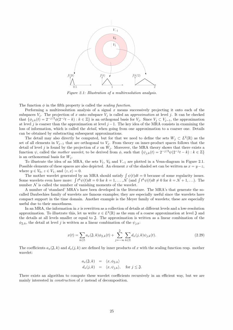
PSfrag replacements
V0
V1
V−1
f (2t) f (t) f (t/2)
210.5
Figure 2.1: Illustration of a multiresolution analysis.
The function φ in the fifth property is called the scaling function.Performing a multiresolution analysis of a signal x means successively projecting it onto each of the
subspaces Vj . The projection of x onto subspace Vj is called an approximation at level j. It can be checkedthat φj,k(t) = 2−j/2φ(2−jt − k) : k ∈ Z is an orthogonal basis for Vj . Since Vj ⊂ Vj−1, the approximationat level j is coarser than the approximation at level j−1. The key idea of the MRA consists in examining theloss of information, which is called the detail, when going from one approximation to a coarser one. Detailscan be obtained by substracting subsequent approximations.
The detail may also directly be computed, but for that we need to define the sets Wj ⊂ L2(R) as theset of all elements in Vj−1 that are orthogonal to Vj . From theory on inner-product spaces follows that thedetail of level j is found by the projection of x on Wj . Moreover, the MRA theory shows that there exists afunction ψ, called the mother wavelet, to be derived from φ, such that ψj,k(t) = 2−j/2ψ(2−jt − k) : k ∈ Zis an orthonormal basis for Wj .
To illustrate the idea of an MRA, the sets V1, V0 and V−1 are plotted in a Venn-diagram in Figure 2.1.Possible elements of these spaces are also depicted. An element x of the shaded set can be written as x = y−z,where y ∈ V0, z ∈ V1, and 〈z, x〉 = 0.
The mother wavelet generated by an MRA should satisfy∫
ψ(t)dt = 0 because of some regularity issues.Some wavelets even have more:
∫
tkψ(t)dt = 0 for k = 1, . . . ,N (and∫
tkψ(t)dt 6= 0 for k = N + 1, . . .). Thenumber N is called the number of vanishing moments of the wavelet.
A number of ‘standard’ MRA’s have been developed in the literature. The MRA’s that generate the so-called Daubechies family of wavelets are famous examples; they are especially useful since the wavelets havecompact support in the time domain. Another example is the Meyer family of wavelets; these are especiallyuseful due to their smoothness.
In an MRA, the information in x is rewritten as a collection of details at different levels and a low-resolutionapproximation. To illustrate this, let us write x ∈ L2(R) as the sum of a coarse approximation at level J andthe details at all levels smaller or equal to J. The approximation is written as a linear combination of theφJ,k, the detail at level j is written as a linear combination of the ψj,k:
x(t) =∑
k∈Z
ax(J, k)φJ,k(t) +
J∑
j=−∞
∑
k∈Z
dx(j, k)ψj,k(t). (2.29)
The coefficients ax(J, k) and dx(j, k) are defined by inner products of x with the scaling function resp. motherwavelet:
ax(J, k) = 〈x, φJ,k〉dx(j, k) = 〈x, ψj,k〉, for j ≤ J.
There exists an algorithm to compute these wavelet coefficients recursively in an efficient way, but we aremainly interested in construction of x instead of decomposition.
25
Application to fractional Brownian motion
In the fractional Brownian motion case, dBH(j, k) is computed by
dBH(j, k) = 〈BH , ψj,k〉 =
∫
R
BH(t)ψj,k(t)dt. (2.30)
Omitting details, the integral is defined as a limit (in L2–norm) of stochastic integrals of approximating simpleprocesses. See Section 1.2.1 for a related procedure.
The covariance structure of dBH(j, k) is studied in Flandrin [29]. The variance of dBH
(j, k) is σ22j(2H+1)
for some constant σ2 > 0. When H > 1/2, the covariances of the wavelet coefficients are quite small, buttheir decay depends heavily on the mother wavelet ψ (mainly through the number of its vanishing moments).Note that the coefficients are (almost) independent if the covariances are very close to zero. As an example,it is shown that the simplest orthonormal wavelet basis, the Haar system (N = 1), for which
ψ(t) =
+1 for 0 ≤ t < 1/2−1 for 1/2 ≤ t < 10 otherwise
,
the assumption of independence of the wavelet coefficients is severely violated. Nevertheless, when a waveletwith more than one vanishing moment is used, the wavelet coefficients are ‘approximately’ independent.
When we want to use the above considerations to simulate fractional Brownian motion, it is natural toanalyze BH(t) in an MRA framework. Note that a finite fractional Brownian motion sample is with probability1 an element of L2(R). An approximate generation method may then be based on (2.29), as suggested inWornell [60]. The author defines the process
BH(t) = limJ→∞
J∑
j=−∞
∑
k∈Z
dBH(j, k)2−j/2ψ(2−jt− k), (2.31)
where dBH(j, k) are independent Gaussian random variables with variance σ22j(2H+1) (the limit in (2.31) is
again to be understood as the limit in L2–norm). The author shows that this process has spectral propertieslike fractional Brownian motion. Therefore, BH is a fractional Brownian motion-like process which can be usedas an approximation for real fractional Brownian motion. In fact, the quality of the approximation improvesas N increases. However, the speed of the method is often affected when a wavelet with more vanishingmoments is chosen. The Daubechies wavelets are widely used; the Daubechies N wavelet has N vanishingmoments, and can be characterized by only 2N numbers, a so-called filter. It can be shown that a waveletcorresponding to a filter of size 2N has at most N vanishing moments, and moreover that the Daubechies Nwavelet is the only wavelet with this property. In practice, the Daubechies 10 wavelet is considered to be agood choice.
It is argued by Abry and Sellan [2] that this method has two major drawbacks. The first is that thecoarsest level approximation is just set to zero, because the infinite sum in (2.31) should be truncated. Theirargument is that the coarse approximation includes the low-frequency behavior of the sample, whereas thedetails describe the high-frequency behavior. Forgetting about the coarse approximation means forgettingabout the long-range dependence and self-similarity, which is clearly not desirable. Moreover, they argue thatthe use of independent wavelet coefficients with orthonormal wavelets results in an approximate correlationstructure.
However, they describe another wavelet-based method that is proposed by Sellan and Meyer [53]. Tounderstand the method, one needs some theory of generalized processes (or tempered distributions). Usingthese notions, one can define a ‘derivative’ of Brownian motion (although its paths are almost surely non-differentiable!). This derivative, sometimes called white noise, can be written as follows:
W (t) =∑
k
µkφ(t− k) +∑
j≤0
∑
k
λj,kψj,k(t), (2.32)
where µk and λj,k are i.i.d. and standard normally distributed. Based on this representation, one obtains afractional Brownian motion in two steps. First, one fractionally integrates (2.32) to obtain a continuous-timeanalog of fractional Gaussian noise (which again only exists in a ‘generalized process’ sense). The resultingprocess is then integrated to get the fractional Brownian motion (in the generalized process sense); a finalargument then shows that this is an ordinary stochastic process with continuous sample paths. For details onfractional integration, we refer to [49].
26
The following representation is obtained from (2.32):
BH(t) =∑
k
bH(k)φ(s)0,k(t) +
∑
j≤0
∑
k
λj,k4−s2jsψ(s)j,k(t), (2.33)
where s = H+1/2, λj,k are again i.i.d. Gaussian random variables, bH(k) is a fractional ARIMA(0, s, 0) process(cf. Section 1.2.3), and φ(s) and ψ(s) are a suitably defined fractional scaling function and wavelet function,
to be derived from φ and ψ. As before, we set φ(s)j,k(t) = 2−j/2φ(s)(2−jt − k) and ψ
(s)j,k(t) = 2−j/2ψ(s)(2−jt −
k). Note that since the first term (the coarse approximation) accounts for the long-term behavior, thisapproximation is expected to have better long-range dependent properties than the Wornell wavelet method.
For the details how to construct these fractional scaling and wavelet function, the reader is referred to[2]. The authors make use of reconstruction algorithms for Riesz bases. Their idea is to calculate the gener-ating sequences of the fractional scaling and wavelet function. These generating sequences fully characterizethe corresponding function. To be precise, the generating sequence for the fractional scaling function resp.fractional wavelet function are the sequences that satisfy
φ(s)(t/2)/√
2 =∑
k
u(s)k φ(s)(t− k)
ψ(s)(t/2)/√
2 =∑
k
v(s)k ψ(s)(t− k).
The generating sequences of the fractional scaling function and wavelet function u(s) and v(s) are computedusing the generating sequences u and v of φ and ψ. The sequences u and v are tabulated, e.g., in [18]. TheARIMA(0, s, 0) process is constructed by manipulating Gaussian white noise using the same techniques thatwere used to compute u(s) from u and v(s) from v. However, this leads to an approximate ARIMA(0, s, 0)sample.
When the coefficients in (2.33) are generated, the so-called fast pyramidal Mallat filter bank algorithmcan be applied to compute (2.33) in an efficient way. For this, the infinite sum has to be truncated at a finitenumber −J . The authors claim to obtain already relevant approximations for J = 5 or J = 6 using theDaubechies 10 wavelet.
As usual, denote the required sample size by N . The finest resolution that is present in a sample of sizeN is determined by 2Jf = N , but a truncation parameter of J = 5 or J = 6 may be interesting to limit thecomputation time. An approximate sample based on (2.33) is found by starting with a fractional ARIMA
sample bH of size N2−J . The sum∑
k bH(k)φ(s)0,k(t) is then computed for t = 2−J , . . . , N2−J . Since the
number of summation terms in∑
k λj,k4−s2jsψ(s)j,k(t) is N2−J−j , this results in an order N2 algorithm when
(2.33) is directly calculated. An additional complication is that no explicit expression for φ(s)(t) exists (evenfor φ and ψ in the Daubechies 10 case it does not exist). However, only the generating sequences need tobe known for the reconstruction, since these sequences serve as input in the pyramidal filter bank algorithm.This algorithm depends heavily on the convolution operation, which can efficiently be implemented using theFast Fourier Transform (FFT). The complexity is then reduced to N logN . Whereas the generating sequenceof the Daubechies 10 wavelet has length 20, the generating sequence of φ(s) and ψ(s) is in general infinite andshould be truncated. Obviously, this has an impact on the speed as well.
There is one more thing to take care of. An important operation in the algorithm is the convolution ofsequences. When convolving two sequences, the begin and end points of the resulting sequence are polluted bythe lack of data; the so-called border effects. These are dealt with by increasing the required sample size witha safety margin and truncating the output sequence (on both sides!). This makes it hard to make theoreticalstatements on the required amount of time. We investigate the time complexity empirically in Chapter 4.
Just before completion of this report, we found some related wavelet decompositions in the literature. InMeyer et al. [43], it is noted that (2.33) is incorrect and that a so-called infrared correction must be added. InChapter 4, we analyze samples simulated using (2.33); the bad performance observed there might be causedby the lack of the infrared correction, although this does not seem to be a plausible explanation. We alsorefer to the recent papers by Ayache and Taqqu [5] and [34] for further details on the wavelet method.
2.2.6 Other methods
Numerous other methods have been proposed as an approximate synthesis method for fractional Brownianmotion. In this section, we will describe a few and discuss their advantages and drawbacks. Of course, thelist is not claimed to be exhaustive.
27
Chaotic maps
The chaotic maps approach (Erramilli et al. [27]) is a method to simulate the source level behavior. Givenan initial random value x0 and a deterministic function f , a deterministic sequence is constructed by therecursion xn+1 = f(xn). The active and inactive periods are determined by the observed sequence, e.g., thesource is active at time n when 0 < xn < 1/2. The chaos (irregular or seemingly stochastic behavior) arisesfrom a property known as Sensitive dependence on Initial Conditions. This means that a small deviation fromthe initial condition results in a completely different sequence. In fact, the absolute difference in xn increasesexponentially in n.
It is shown that simple nonlinear chaotics maps already capture some of the behavior of real teletraffic.However, the maps fail to have a direct interpretation. Therefore, several chaotic maps are tried, hoping thatsatisfactory results for traffic simulation are obtained. Moreover, the output has to be aggregated, whichcauses the same problems as with the Aggregating packet processes approach (see Section 2.2.2).
The Decreusefond and Lavaud method
The Decreusefond and Lavaud method [20] is based on the following representation of fractional Brownianmotion:
BH(t) =
∫ t
0
KH(t, s)dB(s)
for some function KH(t, s), where B denotes ordinary Brownian motion as in Chapter 1.Assume that we need a fractional Brownian motion sample on the interval [0, 1], this interval is then split
in N smaller intervals of equal length. Set tn = n/N for n = 0, 1, . . . , N .We estimate point n of the trace by
BH(tn) =n∑
i=0
1
ti+1 − ti
∫ ti+1
ti
KH(tn, s)ds (B(ti+1) −B(ti)) . (2.34)
The integral∫ ti+1
tiKH(tn, s)ds may not be approximated by KH(tn, ti) or KH(tn, ti+1), because KH(tn, t) is
not continuous with respect to t on [0, tn]. The approximation would then not converge to an exact tracewhen N is large. In [20], the authors describe a rather technical way to overcome this.
Although this method is not really evaluated and tested, the main advantage is clearly that the integral in(2.34) should only be computed once when more than one trace is needed. However, the number of integralsto be calculated is of order N 2 when a sample of length N is needed. All these values should be stored, whichis a drawback of the method. Exact methods that are much faster than this method are also known (seeSection 2.1.3), so the method is not very useful in practice.
The Dzhaparidze and van Zanten methods
Dzhaparidze and van Zanten have proven a number of interesting series representations, as applications ofspectral theory for fractional Brownian motion.
The first [26] involves the positive real zeros x1 < x2 < . . . of the Bessel function J−H of the first kind oforder −H, and the positive zeros y1 < y2 < . . . of J1−H . One then has, in the sense of equality in distribution,
BH(t) =
∞∑
n=1
sinxnt
xnXn +
∞∑
n=1
1 − cos ynt
ynYn,
where X1, X2, . . . and Y1, Y2, . . . are independent centered Gaussian random variables. Their variances aregiven by
VarXn = 2c2Hx−2Hn J−2
1−H(xn), VarYn = 2c2Hy−2Hn J−2
−H(yn),
where c2H = π−1Γ(1+2H) sinπH. Both series converge absolutely and uniformly in t ∈ [0, 1] with probabilityone [26].
The reason why this method is particularly interesting for simulation purposes is that efficient algorithmsexist to compute the zeros of Bessel functions. Moreover, these zeros only have to be computed once, regardlessthe number of traces that need to be simulated. Of course, the series have to be truncated at some level.The question raises what level is appropriate; we do not discuss this issue in this report, but we note that thefollowing estimate holds [25]:
lim supN→∞
NH
√logN
E supt∈[0,1]
∣
∣
∣
∣
∣
∑
n>N
sin xnt
xnXn +
∑
n>N
1 − cos ynt
ynYn
∣
∣
∣
∣
∣
<∞.
28
It turns out that N−H√
logN is the ‘best’ possible rate for a series expansion of fractional Brownian motion[38].
Interestingly, since the xi and yi increase, truncation only concerns the high frequencies. Therefore, themethod is expected to work especially well if the Hurst parameter H is close to one, cf. Figure 1.2. Noticethat the high frequencies (details) are also truncated in the wavelet method.
The second series representation is similar, but only involves the zeros of a single Bessel function, J1−H .For n ∈ N, define σn by
σ−1n =
1 −H
H
Γ2(1 −H)Γ(3/2 −H)
Γ(H + 1/2)Γ(3 − 2H)
(ωn
2
)2H
J2−H(ωn)T 2−2H ,
where ω1 < ω2 < . . . are the positive zeros of J1−H . Let X,Y1, Y2, . . . , Z1, Z2, . . . be i.i.d. standard normalvariables. Then with probability one the series
t√2 − 2H
X +∞∑
n=1
sin 2ωnt/T
ωn/T
√σnYn +
∞∑
n=1
cos 2ωnt/T − 1
ωn/T
√σnZn
converges uniformly in t ∈ [0, T ] and defines a fractional Brownian motion with Hurst parameter H. As thefirst method, one can prove rate-optimality of this expansion.
Appendix: Proof of (2.23)
In this subsection, we prove that for n = 0, 1, 2, . . .:
lim`→∞
∫ π
0
[√
f(λ)
πcos(nλ) − ξ(`)n (λ)
]2
dλ = 0 and (2.35)
lim`→∞
∫ π
0
[√
f(λ)
πsin(nλ) − θ(`)
n (λ)
]2
dλ = 0, (2.36)
where f denotes the spectral density of fractional Gaussian noise for some 0 < H < 1 and (with tk = kπ/`)
ξ(`)n (λ) =
√
f(t1)
πcos(nt1)10(λ) +
`−1∑
k=0
√
f(tk+1)
πcos(ntk+1)1(tk,tk+1](λ) and
θ(`)n (λ) =
√
f(t1)
πsin(nt1)10(λ) +
`−1∑
k=0
√
f(tk+1)
πsin(ntk+1)1(tk,tk+1](λ).
We keep n fixed throughout the proof, and start by showing that θ(`)n converges to θn :=
√
f(λ)π sin(nλ) in
L2–norm as ` → ∞. Note that f has a pole at 0, but that the sine-term compensates this pole. Thus, θn(λ)
is continuous on [0, π] for every Hurst parameter 0 < H < 1. It follows that [θn(λ)]2 is Riemann integrable on
[0, π], which implies that lim`→∞
∫ π
0
[
θ(`)n (λ)
]2
dλ =∫ π
0[θn(λ)]2 dλ. Since θ
(`)n (λ) → θn(λ) for every 0 ≤ λ ≤ π
as `→ ∞, we have the desired convergence of θ(`)n to θn in L2–norm, see for instance Theorem 4.5.4 of Chung
[13].More care is needed to prove (2.35). When 0 < H ≤ 1/2, the same reasoning as above applies. However,
ξn :=√
f(λ)π cos(nλ) has a pole at 0 for 1/2 < H < 1. Still, f is (Riemann) integrable because f is a spectral
density; in fact,∫ π
0f(λ)dλ = π. For any ε > 0, this makes it possible to find a δ > 0 (independent of `) such
that
∫ δ
0
[
ξ(`)n (λ) − ξn(λ)]2
dλ ≤∫ δ
0
[
ξ(`)n (λ) + ξn(λ)]2
dλ ≤ 4
∫ δ
0
[ξn(λ)]2 dλ
≤ 4
∫ δ
0
f(λ)dλ < ε/2,
where the first two inequalities use the fact that ξn(λ) ≥ ξ(`)n (λ) ≥ 0 for small λ. As before, we have
ξ(`)n (λ) → ξn(λ) for every δ ≤ λ ≤ π, and the Riemann integrability of [ξn(λ)]2 on [δ, π], which implies
29
that lim`→∞
∫ π
δ
[
ξ(`)n (λ)
]2
dλ =∫ π
δ[ξn(λ)]2 dλ. Hence, it is possible to find an ` with the property that
∫ π
δ
[
ξ(`)n (λ) − ξn(λ)
]2
dλ < ε/2 and the claim is proven.
Note that the arguments of the proof apply for a general spectral density, not necessarily the spectraldensity of fGn.
30
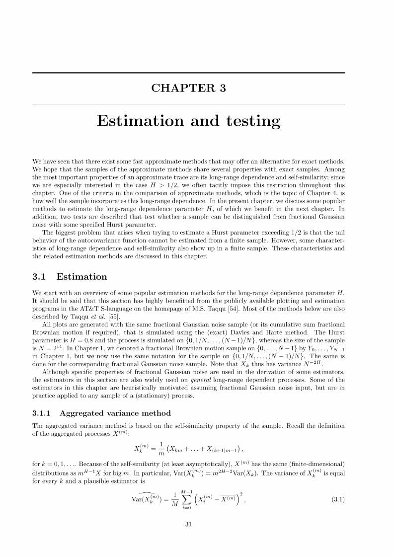
CHAPTER 3
Estimation and testing
We have seen that there exist some fast approximate methods that may offer an alternative for exact methods.We hope that the samples of the approximate methods share several properties with exact samples. Amongthe most important properties of an approximate trace are its long-range dependence and self-similarity; sincewe are especially interested in the case H > 1/2, we often tacitly impose this restriction throughout thischapter. One of the criteria in the comparison of approximate methods, which is the topic of Chapter 4, ishow well the sample incorporates this long-range dependence. In the present chapter, we discuss some popularmethods to estimate the long-range dependence parameter H, of which we benefit in the next chapter. Inaddition, two tests are described that test whether a sample can be distinguished from fractional Gaussiannoise with some specified Hurst parameter.
The biggest problem that arises when trying to estimate a Hurst parameter exceeding 1/2 is that the tailbehavior of the autocovariance function cannot be estimated from a finite sample. However, some character-istics of long-range dependence and self-similarity also show up in a finite sample. These characteristics andthe related estimation methods are discussed in this chapter.
3.1 Estimation
We start with an overview of some popular estimation methods for the long-range dependence parameter H.It should be said that this section has highly benefitted from the publicly available plotting and estimationprograms in the AT&T S-language on the homepage of M.S. Taqqu [54]. Most of the methods below are alsodescribed by Taqqu et al. [55].
All plots are generated with the same fractional Gaussian noise sample (or its cumulative sum fractionalBrownian motion if required), that is simulated using the (exact) Davies and Harte method. The Hurstparameter is H = 0.8 and the process is simulated on 0, 1/N, . . . , (N −1)/N, whereas the size of the sampleis N = 214. In Chapter 1, we denoted a fractional Brownian motion sample on 0, . . . , N−1 by Y0, . . . , YN−1
in Chapter 1, but we now use the same notation for the sample on 0, 1/N, . . . , (N − 1)/N. The same isdone for the corresponding fractional Gaussian noise sample. Note that Xk thus has variance N−2H .
Although specific properties of fractional Gaussian noise are used in the derivation of some estimators,the estimators in this section are also widely used on general long-range dependent processes. Some of theestimators in this chapter are heuristically motivated assuming fractional Gaussian noise input, but are inpractice applied to any sample of a (stationary) process.
3.1.1 Aggregated variance method
The aggregated variance method is based on the self-similarity property of the sample. Recall the definitionof the aggregated processes X(m):
X(m)k =
1
m
(
Xkm + . . .+X(k+1)m−1
)
,
for k = 0, 1, . . .. Because of the self-similarity (at least asymptotically), X (m) has the same (finite-dimensional)
distributions as mH−1X for big m. In particular, Var(X(m)k ) = m2H−2Var(Xk). The variance of X
(m)k is equal
for every k and a plausible estimator is
Var(X
(m)k ) =
1
M
M−1∑
i=0
(
X(m)i −X(m)
)2
, (3.1)
31
0.0 0.5 1.0 1.5 2.0 2.5 3.0 3.5
−1.5
−1.0
−0.5
0.0
PSfrag
replacem
ents
log10(m)
log 1
0
(
V
ar(X
(m)
k))
Figure 3.1: The aggregated variance method.
where X(m) denotes the sample average of X(m):
X(m) =1
M
M−1∑
i=0
X(m)i .
In both formulas, M is the integer part of N/m. The estimator of H is obtained by plotting
Var(X(m)k ) versus
m on a log-log scale. When the estimates of the variances were equal to their real values, all the points wouldlie on a straight line with slope 2H − 2. In practice, the slope is estimated by fitting a straight line throughthe points. The estimate for H is found from the estimate of the slope.
However, this is very naive, since estimator (3.1) is biased in the presence of non-zero correlations, partic-ularly long-range dependence. It is pointed out in Beran [9] that this bias disappears when M is large (i.e.,N is large and m is small), but that this happens very slowly for samples with long-range dependence. Infact, it holds that
E
(
Var(X
(m)k )
)
∼ Var(X(m)k )
[
1 − CM2H−2]
, (3.2)
for some constant C and M → ∞. In the presence of positive correlations (i.e., H > 1/2), C is positive
and
Var(X(m)k ) tends to underestimate Var(X
(m)k ) for small M . This leads also to an underestimate of H
(assuming that the estimator of the slope is not too much biased). Moreover, we see that this bias increasesin H, which is also found in the empirical study by Taqqu et al. [55].
In addition to the already mentioned problems for small M (i.e., ‘large’ m), the estimates of the variancesare based on only few observations and therefore unreliable. To avoid these observations from spoiling theestimate for H, those estimates are simply not used in the fitting procedure. The same is done for theobservations for ‘small’ m, because those may be based on the short-term correlation structure (althoughthese are high-quality estimates if no short-range dependence is present, as in the fractional Gaussian noisecase).
From the theory on least-squares fitting, it is known that the estimator of the slope (and thus for H)is unbiased under some conditions on the so-called disturbance term. Among others, the independence and
normality of log
(
Var(X
(m)k )
)
for a range of values of m should be studied in more detail. If m is large (M
small), the normality is questionable, see (3.1). Independence will not occur in general, since the whole series
is used to compute
Var(X(m)k ) for every m. Because all line-fitting estimators in this chapter share these
problems, they are all biased.In Figure 3.1, the log-log plot is given for our sample. The observations that are used in the fitting of
the line are dotted. From this plot, the estimated Hurst parameter is 0.7889, quite close to the real valueof 0.8. As expected, the estimate is indeed lower than its real value. A weakness of the method is thatthe fitting region may arbitrarily be chosen (in our plot from 0.7 to 2.5 on a log10 scale), which results in anon-robust estimate. For our sample, the estimated variances for small m lie also on the fitted line, becauseour sample was an exact fractional Gaussian noise sample without special short-term behavior. The dashedline corresponds to a Hurst parameter of 0.5.
32
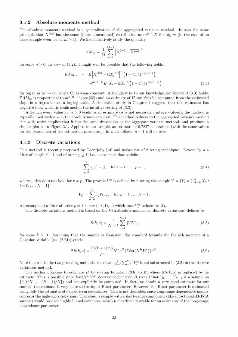
3.1.2 Absolute moments method
The absolute moments method is a generalization of the aggregated variance method. It uses the sameprinciple that X(m) has the same (finite-dimensional) distribution as mH−1X for big m (in the case of anexact sample even for all m ≥ 1). We first intuitively study the quantity
AMm =1
M
M−1∑
i=0
∣
∣
∣X
(m)i −X(m)
∣
∣
∣
n
for some n > 0. In view of (3.2), it might well be possible that the following holds:
EAMm ∼ E
∣
∣
∣X
(m)i − EX
(m)i
∣
∣
∣
n (
1 − CnMn(H−1)
)
= mn(H−1)E |Xi − EXi|n(
1 − CnMn(H−1)
)
, (3.3)
for big m as M → ∞, where Cn is some constant. Although it is, to our knowledge, not known if (3.3) holds,EAMm is proportional to mn(H−1) (see [55]) and an estimate of H can thus be computed from the estimatedslope in a regression on a log-log scale. A simulation study in Chapter 4 suggests that this estimator hasnegative bias, which is confirmed in the intuitive setting of (3.3).
Although every value for n > 0 leads to an estimate (n is not necessarily integer-valued), the method istypically used with n = 1, the absolute moments case. The method reduces to the aggregated variance methodif n = 2, which implies that it has the same drawbacks as the aggregate variance method, and produces asimilar plot as in Figure 3.1. Applied to our sample, an estimate of 0.7827 is obtained (with the same valuesfor the parameters of the estimation procedure). In what follows, n = 1 will be used.
3.1.3 Discrete variations
This method is recently proposed by Coeurjolly [14] and makes use of filtering techniques. Denote by a afilter of length `+ 1 and of order p ≥ 1, i.e., a sequence that satisfies
∑
q=0
aqqr = 0, for r = 0, . . . , p− 1, (3.4)
whereas this does not hold for r = p. The process V a is defined by filtering the sample Y = Yi =∑i
k=0Xk :i = 0, . . . , N − 1:
V ak =
∑
q=0
aqYk−q, for k = `, . . . , N − 1.
An example of a filter of order p = 1 is a = (−1, 1), in which case V ak reduces to Xk.
The discrete variations method is based on the k-th absolute moment of discrete variations, defined by
S(k, a) =1
N − `
N−1∑
i=`
|V ai |k , (3.5)
for some k > 0. Assuming that the sample is Gaussian, the standard formula for the kth moment of aGaussian variable (see (2.24)) yields
ES(k, a) =Γ((k + 1)/2)√
πN−kH2Var(NHV a
1 )k/2. (3.6)
Note that unlike the two preceding methods, the mean 1N−`
∑N−1i=` V a
i is not substracted in (3.5) in the discretevariations method.
The author proposes to estimate H by solving Equation (3.6) to H, where ES(k, a) is replaced by itsestimate. This is possible since Var(NHV a
1 ) does not depend on H (recall that Y0, . . . , YN−1 is a sample on0, 1/N, . . . , (N − 1)/N) and can explicitly be computed. In fact, we obtain a very good estimate for oursample; the estimate is very close to the input Hurst parameter. However, the Hurst parameter is estimatedusing only the estimates of ` short term covariances. This is not desirable, since long-range dependence mainlyconcerns the high-lag correlations. Therefore, a sample with a short-range component (like a fractional ARIMAsample) would produce highly biased estimates, which is clearly undesirable for an estimator of the long-rangedependence parameter.
33
0.5 1.0 1.5 2.0 2.5 3.0
−6−5
−4−3
PSfrag
replacem
ents
log10(m)
log 1
0(S
(k,a
))
Figure 3.2: The discrete variations method.
A second estimation method that is based on S(k, a) (also proposed in [14]) can be regarded as a gen-eralization of the absolute moments method. Let us define the sequence of filters (am)1≤m≤M for some Mby
ami =
aj for i = jm0 otherwise
.
Using (3.4) and (3.6) for r = 0, it is readily checked that ES(k, am) = mHkES(k, a). An estimator of H isthus deduced from a linear regression of log S(k, am) : 1 ≤ m ≤ M on k log(m) : 1 ≤ m ≤ M. Thismethod reduces to the absolute moments method for a = (−1, 1) (up to the substraction of the mean, whichis close to zero).
More importantly, the author proves that this estimator converges at a rate of√N to a zero-mean Gaussian
distribution with variance σ2(k, a) for some σ2(k, a) > 0. He also shows that this variance is minimal fork = 2. Although it is not clear that we can neglect the influence of the substraction of the mean, this suggeststhat the estimator of the method of moments is inferior to the estimator of the method of aggregated variance,possibly only for large sample sizes.
Note that it is assumed that the sample is Gaussian, or at least that (3.6) holds for a given k. Theperformance of this method has not been investigated for non-Gaussian samples, but this is no problem forour fractional Brownian motion setting.
To eliminate the impact of short term behavior on the estimator, it is also possible to use only the filtersam with M1 ≤ m ≤ M2 for some M1,M2 in the regression. Applied to our sample, this produces a plot asgiven in Figure 3.2. The bounds M1 and M2 are chosen as in Section 3.1.1, whereas the used filter is theDaubechies 4 filter (see Daubechies [18]) for which p = 2. The resulting estimate for the Hurst parameter is0.7913 (k = 2).
3.1.4 The Higuchi method
As suggested by its name, this method was proposed by Higuchi [31]. The method is quite similar to themethod of absolute moments with n = 1. Instead of using non-intersecting blocks, a sliding window is used,which makes the method computationally much more intensive than the above methods.
The quantity on which the Higuchi method is based is
L(m) =N − 1
m3
m∑
i=1
1
Mi
Mi∑
k=1
∣
∣
∣
∣
∣
∣
i+km∑
j=i+(k−1)m+1
Xj
∣
∣
∣
∣
∣
∣
,
where Mi signifies the integer part of (N − i)/m. The estimate of H is found by plotting L(m) in a log-logplot versus m and adding 2 to the slope of the fitted straight line.
Again, small and large values of m should not be used in the fitting. For our sample, the method gives anestimate of 0.7865, see Figure 3.3.
3.1.5 Periodogram method
The periodogram method estimates the Hurst parameter by fitting a straight line in the spectral domain.This is based on the observation that the spectral density (1.11) behaves like cf |λ|1−2H for |λ| → 0.
34
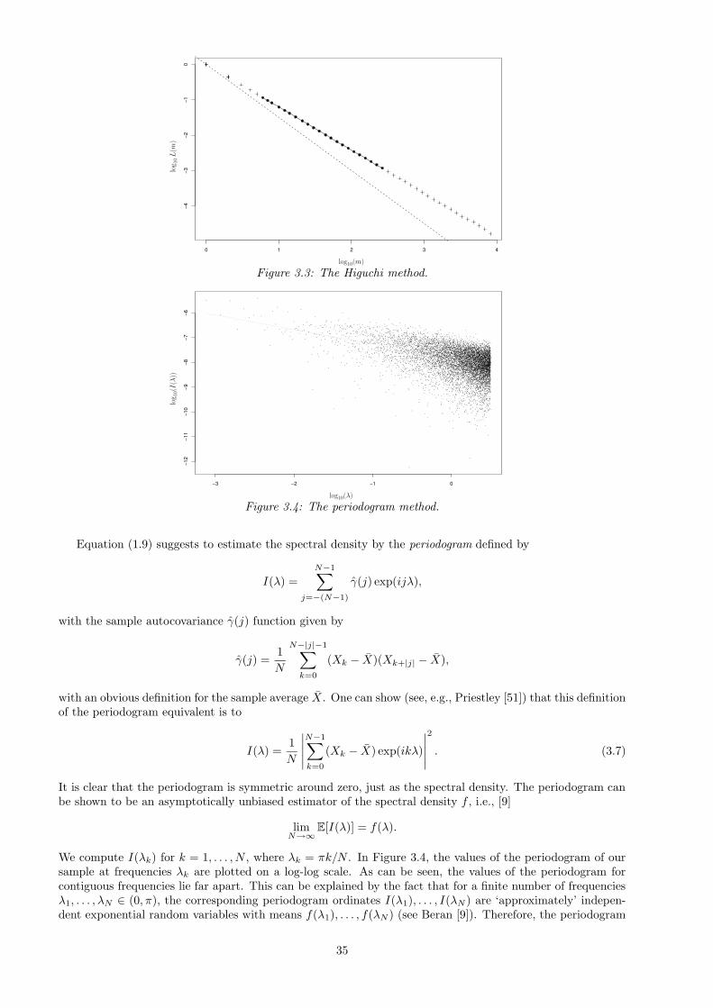
0 1 2 3 4
−4−3
−2−1
0
PSfrag
replacem
ents
log10(m)
log 1
0L
(m)
Figure 3.3: The Higuchi method.
−3 −2 −1 0
−12
−11
−10
−9−8
−7−6
PSfrag
replacem
ents
log10 (m
)
log10(λ)
log 1
0(I
(λ))
Figure 3.4: The periodogram method.
Equation (1.9) suggests to estimate the spectral density by the periodogram defined by
I(λ) =N−1∑
j=−(N−1)
γ(j) exp(ijλ),
with the sample autocovariance γ(j) function given by
γ(j) =1
N
N−|j|−1∑
k=0
(Xk − X)(Xk+|j| − X),
with an obvious definition for the sample average X. One can show (see, e.g., Priestley [51]) that this definitionof the periodogram equivalent is to
I(λ) =1
N
∣
∣
∣
∣
∣
N−1∑
k=0
(Xk − X) exp(ikλ)
∣
∣
∣
∣
∣
2
. (3.7)
It is clear that the periodogram is symmetric around zero, just as the spectral density. The periodogram canbe shown to be an asymptotically unbiased estimator of the spectral density f , i.e., [9]
limN→∞
E[I(λ)] = f(λ).
We compute I(λk) for k = 1, . . . , N , where λk = πk/N . In Figure 3.4, the values of the periodogram of oursample at frequencies λk are plotted on a log-log scale. As can be seen, the values of the periodogram forcontiguous frequencies lie far apart. This can be explained by the fact that for a finite number of frequenciesλ1, . . . , λN ∈ (0, π), the corresponding periodogram ordinates I(λ1), . . . , I(λN ) are ‘approximately’ indepen-dent exponential random variables with means f(λ1), . . . , f(λN ) (see Beran [9]). Therefore, the periodogram
35
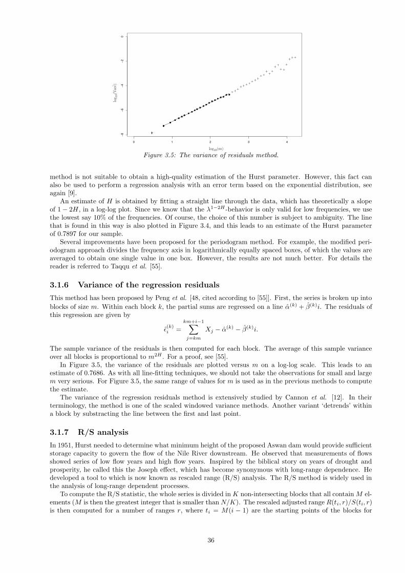
0 1 2 3 4
−8−6
−4−2
0
PSfrag
replacem
ents
log10(m)
log 1
0(V
ar¯ ε)
Figure 3.5: The variance of residuals method.
method is not suitable to obtain a high-quality estimation of the Hurst parameter. However, this fact canalso be used to perform a regression analysis with an error term based on the exponential distribution, seeagain [9].
An estimate of H is obtained by fitting a straight line through the data, which has theoretically a slopeof 1 − 2H, in a log-log plot. Since we know that the λ1−2H -behavior is only valid for low frequencies, we usethe lowest say 10% of the frequencies. Of course, the choice of this number is subject to ambiguity. The linethat is found in this way is also plotted in Figure 3.4, and this leads to an estimate of the Hurst parameterof 0.7897 for our sample.
Several improvements have been proposed for the periodogram method. For example, the modified peri-odogram approach divides the frequency axis in logarithmically equally spaced boxes, of which the values areaveraged to obtain one single value in one box. However, the results are not much better. For details thereader is referred to Taqqu et al. [55].
3.1.6 Variance of the regression residuals
This method has been proposed by Peng et al. [48, cited according to [55]]. First, the series is broken up into
blocks of size m. Within each block k, the partial sums are regressed on a line α(k) + β(k)i. The residuals ofthis regression are given by
ε(k)i =
km+i−1∑
j=km
Xj − α(k) − β(k)i.
The sample variance of the residuals is then computed for each block. The average of this sample varianceover all blocks is proportional to m2H . For a proof, see [55].
In Figure 3.5, the variance of the residuals are plotted versus m on a log-log scale. This leads to anestimate of 0.7686. As with all line-fitting techniques, we should not take the observations for small and largem very serious. For Figure 3.5, the same range of values for m is used as in the previous methods to computethe estimate.
The variance of the regression residuals method is extensively studied by Cannon et al. [12]. In theirterminology, the method is one of the scaled windowed variance methods. Another variant ‘detrends’ withina block by substracting the line between the first and last point.
3.1.7 R/S analysis
In 1951, Hurst needed to determine what minimum height of the proposed Aswan dam would provide sufficientstorage capacity to govern the flow of the Nile River downstream. He observed that measurements of flowsshowed series of low flow years and high flow years. Inspired by the biblical story on years of drought andprosperity, he called this the Joseph effect, which has become synonymous with long-range dependence. Hedeveloped a tool to which is now known as rescaled range (R/S) analysis. The R/S method is widely used inthe analysis of long-range dependent processes.
To compute the R/S statistic, the whole series is divided in K non-intersecting blocks that all contain M el-ements (M is then the greatest integer that is smaller than N/K). The rescaled adjusted range R(ti, r)/S(ti, r)is then computed for a number of ranges r, where ti = M(i − 1) are the starting points of the blocks for
36
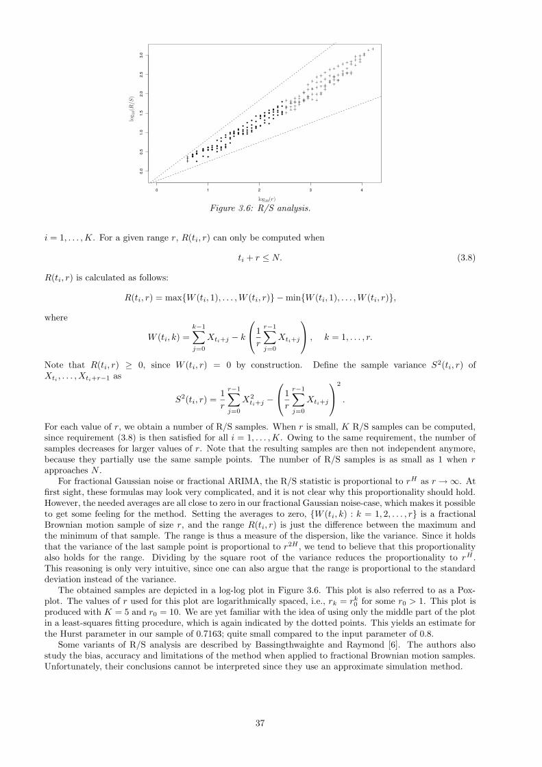
0 1 2 3 4
0.0
0.5
1.0
1.5
2.0
2.5
3.0
PSfrag
replacem
ents
log10 (m
)
log10(r)
log 1
0(R
/S)
Figure 3.6: R/S analysis.
i = 1, . . . ,K. For a given range r, R(ti, r) can only be computed when
ti + r ≤ N. (3.8)
R(ti, r) is calculated as follows:
R(ti, r) = maxW (ti, 1), . . . ,W (ti, r) − minW (ti, 1), . . . ,W (ti, r),
where
W (ti, k) =k−1∑
j=0
Xti+j − k
1
r
r−1∑
j=0
Xti+j
, k = 1, . . . , r.
Note that R(ti, r) ≥ 0, since W (ti, r) = 0 by construction. Define the sample variance S2(ti, r) ofXti
, . . . , Xti+r−1 as
S2(ti, r) =1
r
r−1∑
j=0
X2ti+j −
1
r
r−1∑
j=0
Xti+j
2
.
For each value of r, we obtain a number of R/S samples. When r is small, K R/S samples can be computed,since requirement (3.8) is then satisfied for all i = 1, . . . ,K. Owing to the same requirement, the number ofsamples decreases for larger values of r. Note that the resulting samples are then not independent anymore,because they partially use the same sample points. The number of R/S samples is as small as 1 when rapproaches N .
For fractional Gaussian noise or fractional ARIMA, the R/S statistic is proportional to rH as r → ∞. Atfirst sight, these formulas may look very complicated, and it is not clear why this proportionality should hold.However, the needed averages are all close to zero in our fractional Gaussian noise-case, which makes it possibleto get some feeling for the method. Setting the averages to zero, W (ti, k) : k = 1, 2, . . . , r is a fractionalBrownian motion sample of size r, and the range R(ti, r) is just the difference between the maximum andthe minimum of that sample. The range is thus a measure of the dispersion, like the variance. Since it holdsthat the variance of the last sample point is proportional to r2H , we tend to believe that this proportionalityalso holds for the range. Dividing by the square root of the variance reduces the proportionality to rH .This reasoning is only very intuitive, since one can also argue that the range is proportional to the standarddeviation instead of the variance.
The obtained samples are depicted in a log-log plot in Figure 3.6. This plot is also referred to as a Pox-plot. The values of r used for this plot are logarithmically spaced, i.e., rk = rk
0 for some r0 > 1. This plot isproduced with K = 5 and r0 = 10. We are yet familiar with the idea of using only the middle part of the plotin a least-squares fitting procedure, which is again indicated by the dotted points. This yields an estimate forthe Hurst parameter in our sample of 0.7163; quite small compared to the input parameter of 0.8.
Some variants of R/S analysis are described by Bassingthwaighte and Raymond [6]. The authors alsostudy the bias, accuracy and limitations of the method when applied to fractional Brownian motion samples.Unfortunately, their conclusions cannot be interpreted since they use an approximate simulation method.
37
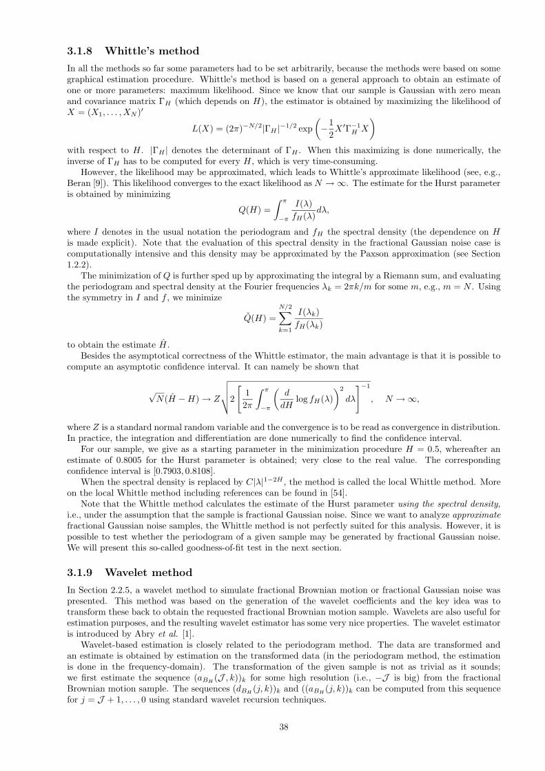
3.1.8 Whittle’s method
In all the methods so far some parameters had to be set arbitrarily, because the methods were based on somegraphical estimation procedure. Whittle’s method is based on a general approach to obtain an estimate ofone or more parameters: maximum likelihood. Since we know that our sample is Gaussian with zero meanand covariance matrix ΓH (which depends on H), the estimator is obtained by maximizing the likelihood ofX = (X1, . . . , XN )′
L(X) = (2π)−N/2|ΓH |−1/2 exp
(
−1
2X ′Γ−1
H X
)
with respect to H. |ΓH | denotes the determinant of ΓH . When this maximizing is done numerically, theinverse of ΓH has to be computed for every H, which is very time-consuming.
However, the likelihood may be approximated, which leads to Whittle’s approximate likelihood (see, e.g.,Beran [9]). This likelihood converges to the exact likelihood as N → ∞. The estimate for the Hurst parameteris obtained by minimizing
Q(H) =
∫ π
−π
I(λ)
fH(λ)dλ,
where I denotes in the usual notation the periodogram and fH the spectral density (the dependence on His made explicit). Note that the evaluation of this spectral density in the fractional Gaussian noise case iscomputationally intensive and this density may be approximated by the Paxson approximation (see Section1.2.2).
The minimization of Q is further sped up by approximating the integral by a Riemann sum, and evaluatingthe periodogram and spectral density at the Fourier frequencies λk = 2πk/m for some m, e.g., m = N . Usingthe symmetry in I and f , we minimize
Q(H) =
N/2∑
k=1
I(λk)
fH(λk)
to obtain the estimate H .Besides the asymptotical correctness of the Whittle estimator, the main advantage is that it is possible to
compute an asymptotic confidence interval. It can namely be shown that
√N(H −H) → Z
√
√
√
√2
[
1
2π
∫ π
−π
(
d
dHlog fH(λ)
)2
dλ
]−1
, N → ∞,
where Z is a standard normal random variable and the convergence is to be read as convergence in distribution.In practice, the integration and differentiation are done numerically to find the confidence interval.
For our sample, we give as a starting parameter in the minimization procedure H = 0.5, whereafter anestimate of 0.8005 for the Hurst parameter is obtained; very close to the real value. The correspondingconfidence interval is [0.7903, 0.8108].
When the spectral density is replaced by C|λ|1−2H , the method is called the local Whittle method. Moreon the local Whittle method including references can be found in [54].
Note that the Whittle method calculates the estimate of the Hurst parameter using the spectral density,i.e., under the assumption that the sample is fractional Gaussian noise. Since we want to analyze approximatefractional Gaussian noise samples, the Whittle method is not perfectly suited for this analysis. However, it ispossible to test whether the periodogram of a given sample may be generated by fractional Gaussian noise.We will present this so-called goodness-of-fit test in the next section.
3.1.9 Wavelet method
In Section 2.2.5, a wavelet method to simulate fractional Brownian motion or fractional Gaussian noise waspresented. This method was based on the generation of the wavelet coefficients and the key idea was totransform these back to obtain the requested fractional Brownian motion sample. Wavelets are also useful forestimation purposes, and the resulting wavelet estimator has some very nice properties. The wavelet estimatoris introduced by Abry et al. [1].
Wavelet-based estimation is closely related to the periodogram method. The data are transformed andan estimate is obtained by estimation on the transformed data (in the periodogram method, the estimationis done in the frequency-domain). The transformation of the given sample is not as trivial as it sounds;we first estimate the sequence (aBH
(J , k))k for some high resolution (i.e., −J is big) from the fractionalBrownian motion sample. The sequences (dBH
(j, k))k and ((aBH(j, k))k can be computed from this sequence
for j = J + 1, . . . , 0 using standard wavelet recursion techniques.
38
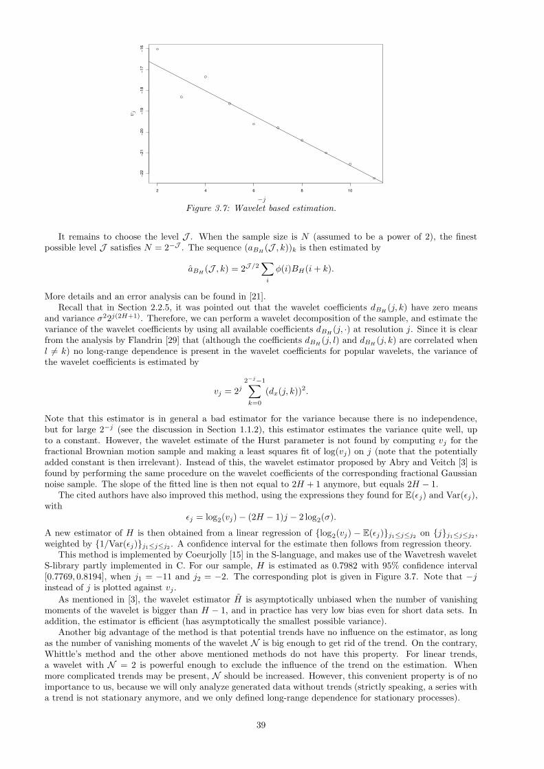
2 4 6 8 10
−22
−21
−20
−19
−18
−17
−16
PSfrag
replacem
ents
log10 (m
)
v j
−j
Figure 3.7: Wavelet based estimation.
It remains to choose the level J . When the sample size is N (assumed to be a power of 2), the finestpossible level J satisfies N = 2−J . The sequence (aBH
(J , k))k is then estimated by
aBH(J , k) = 2J /2
∑
i
φ(i)BH(i+ k).
More details and an error analysis can be found in [21].Recall that in Section 2.2.5, it was pointed out that the wavelet coefficients dBH
(j, k) have zero meansand variance σ22j(2H+1). Therefore, we can perform a wavelet decomposition of the sample, and estimate thevariance of the wavelet coefficients by using all available coefficients dBH
(j, ·) at resolution j. Since it is clearfrom the analysis by Flandrin [29] that (although the coefficients dBH
(j, l) and dBH(j, k) are correlated when
l 6= k) no long-range dependence is present in the wavelet coefficients for popular wavelets, the variance ofthe wavelet coefficients is estimated by
vj = 2j2−j−1∑
k=0
(dx(j, k))2.
Note that this estimator is in general a bad estimator for the variance because there is no independence,but for large 2−j (see the discussion in Section 1.1.2), this estimator estimates the variance quite well, upto a constant. However, the wavelet estimate of the Hurst parameter is not found by computing vj for thefractional Brownian motion sample and making a least squares fit of log(vj) on j (note that the potentiallyadded constant is then irrelevant). Instead of this, the wavelet estimator proposed by Abry and Veitch [3] isfound by performing the same procedure on the wavelet coefficients of the corresponding fractional Gaussiannoise sample. The slope of the fitted line is then not equal to 2H + 1 anymore, but equals 2H − 1.
The cited authors have also improved this method, using the expressions they found for E(εj) and Var(εj),with
εj = log2(vj) − (2H − 1)j − 2 log2(σ).
A new estimator of H is then obtained from a linear regression of log2(vj) − E(εj)j1≤j≤j2 on jj1≤j≤j2 ,weighted by 1/Var(εj)j1≤j≤j2 . A confidence interval for the estimate then follows from regression theory.
This method is implemented by Coeurjolly [15] in the S-language, and makes use of the Wavetresh waveletS-library partly implemented in C. For our sample, H is estimated as 0.7982 with 95% confidence interval[0.7769, 0.8194], when j1 = −11 and j2 = −2. The corresponding plot is given in Figure 3.7. Note that −jinstead of j is plotted against vj .
As mentioned in [3], the wavelet estimator H is asymptotically unbiased when the number of vanishingmoments of the wavelet is bigger than H − 1, and in practice has very low bias even for short data sets. Inaddition, the estimator is efficient (has asymptotically the smallest possible variance).
Another big advantage of the method is that potential trends have no influence on the estimator, as longas the number of vanishing moments of the wavelet N is big enough to get rid of the trend. On the contrary,Whittle’s method and the other above mentioned methods do not have this property. For linear trends,a wavelet with N = 2 is powerful enough to exclude the influence of the trend on the estimation. Whenmore complicated trends may be present, N should be increased. However, this convenient property is of noimportance to us, because we will only analyze generated data without trends (strictly speaking, a series witha trend is not stationary anymore, and we only defined long-range dependence for stationary processes).
39

3.2 Testing
Except for a few estimators, the estimation methods described in the previous section can be used to estimatethe Hurst parameter of general long-range dependent samples. In this section on testing techniques, wefocus on fractional Gaussian noise. It is possible to test statistically if our sample can be distinguished fromfractional Gaussian noise. One could think that this is precisely what we need to evaluate simulation methodsof fractional Gaussian noise and fractional Brownian motion, and thus question why all above mentionedestimation methods are needed for our analysis. Before we discuss this, we need to know more about thehypotheses of the tests.
We will study two tests. The null hypothesis is in one case that the spectral density is given by (1.11), inthe other case that the covariances of the sample are in accordance with fractional Gaussian noise for somespecified Hurst parameter; in both cases, the alternative is that the null hypothesis does not hold. This is thefirst drawback, because a test where the null and alternative hypothesis are swapped is much more powerful.We would then have statistical evidence against the hypothesis that the sample is not fractional Gaussiannoise.
Moreover, it is unimaginable to summarize the sample in one number (the test statistic or p-value) andnot to lose information on how it was produced. Therefore, it is still useful to have a look at the othermethods that estimate the long-range dependence parameter H. By doing this, it is easier to find out whatthe particular weaknesses of the simulation method are; every estimation method is namely based on someproperty that a ‘proper’ fractional Gaussian noise (or fractional Brownian motion) sample should have. Inother words, we get some feeling for the approximate methods when we see which properties are incorporatedin the sample and which are not.
When two approximate methods are performing quite well, we cannot value the two methods by meansof the test statistic or its p-value of only one sample, because this value is subject to coincidence. This is anadditional problem in the use of these tests, which makes it necessary to extract more information from thesample. In fact, we can also exploit the possibility that we can generate as many samples as we like. Theconclusions of the tests are then more robust.
3.2.1 A goodness-of-fit test for the spectral density
Beran [8] proposed a goodness-of-fit test statistic based on the spectral properties in the sample. In fact, it istested whether the sample spectral density (i.e., the periodogram) could be generated by a process with somespecified spectral density (which is in our case the spectral density of fractional Gaussian noise with the trueH).
However, some problems are involved when this is tested. The observed frequencies in the sample arecompared to the expected spectral information contained in f , but nothing is said about the distribution ofthese frequencies in time. Therefore, it is possible that a non-stationary series has spectral properties thatforce the test to accept the null hypothesis.
Moreover, the comparison of spectral densities involves only the correlation structure. Recall that thespectral density is defined as fH(λ) =
∑∞j=−∞ γ(j) exp(ijλ), where γ(·) is the autocovariance function (note
that the dependence on H is again made explicit in the notation). Therefore, it is possible to have a non-centered process that has exactly the same spectral density as fractional Gaussian noise. In addition, somenon-Gaussian process may also have the same spectral density. However, this is no problem in our setup,since it is clear from the structure of all approximate generation methods under consideration that a Gaussianzero-mean sample is produced.
The goodness-of-fit statistic is defined as
TN (H) =AN (H)
BN (H)2, (3.9)
where
AN (H) =4π
N
N/2∑
k=1
I(λk)
fH(λk)
2
and BN (H) =
4π
N
N/2∑
k=1
I(λk)
fH(λk)
2
.
Here, I(·) denotes the periodogram (see (3.7)) of the observed data and fH(·) the spectral density of fractionalGaussian noise with the real H. Both are evaluated at the Fourier frequencies λk = 2πk/N .
It is shown in [8] that, under the null hypothesis,√N(AN (H)−µ1, BN (H)−µ2) converges in distribution
to a bivariate Gaussian random variable with mean 0 and covariance matrix Σ as N → ∞ for some knownµ1, µ2 and Σ. Using the so-called Delta method, the author deduces that TN (H) is approximately normally
40
distributed with mean π−1 and variance 2π−2N−1. It is claimed that the approximation of TN (H) by such aGaussian random variable is already good for moderately large sample sizes.
From a practical point of view, one of the strengths of this goodness-of-fit test is that the asymptoticdistribution of the test statistic is not affected when the Whittle estimated Hurst parameter is substituted in(3.9), see again [8]. However, this is of no importance to us, since we are interested whether an approximatesample can be distinguished from fractional Gaussian noise with the input Hurst parameter.
Beran has also implemented this test, and made the code publicly available. For our sample, the teststatistic is 0.3213, which corresponds to an asymptotic p-value of 0.3916 (i.e., in this case 2P (TN (H) >0.3213) = 0.3916, since the test is two-sided). This means that the null hypothesis of a spectral density withHurst parameter H = 0.8 is accepted at any reasonable confidence level. Recall that the p-value has to becompared with a given confidence level, e.g., 5%.
However, testing whether this sample is fractional Gaussian noise with Hurst parameter 0.76 leads to ap-value of 0.1158, still accepting the null hypothesis even at a 10% confidence level. This makes us slightlysuspicious about the power of this test.
3.2.2 A chi-square test for fractional Gaussian noise
As indicated in the discussion of the goodness-of-fit test for the spectral density, it is desirable to testwhether the finite-dimensional distributions are in accordance with fractional Gaussian noise. Althoughseveral goodness-of-fit tests exist to test the marginal distribution [9, Sec. 10.1], we restrict ourselves to achi-square test for the joint distribution. Under the null hypothesis, the sample has zero mean and its auto-covariance function γ(·) is given by (1.7). Recall from Chapter 2 that the covariance matrix Γ determined byγ(·) has a Cholesky decomposition Γ = LL′. Denoting again the sample size by N , we can ‘standardize’ a frac-tional Gaussian noise sample X = (X0, . . . , XN−1)
′ by computing Z = L−1X, such that Z has independentstandard normal elements. A chi-square test can be based on this fact.
Letting Z = (Z0, . . . , ZN−1), the test statistic is
CN (H) =
N−1∑
k=0
Z2k , (3.10)
which is chi-square distributed with N degrees of freedom under the null hypothesis. Again, the dependenceon H is emphasized in the notation (note that Γ and therefore L also depend on H). For a given confidencelevel α, the hypothesis is rejected when CN (H) is larger than the upper α-quantile of the χ2
N distribution.Unlike the goodness-of-fit test, it is (to our knowledge) not known if the asymptotic distribution of the
test statistic is affected when Z is computed by substituting a consistent estimator H for H: more researchhas to be done to see if
CN (H) −N√2N
converges in distribution to a standard normal variable as N → ∞.The power of the test against alternatives can also be studied in more detail. It is a desirable property
of a test that the distribution of the test statistic under alternatives is very different from the distributionunder the null hypothesis. The null hypothesis is then rejected with a relatively high probability when thealternative is true. This is called the power of the test. In other words, it is desirable that the distribution ofCN (H) ‘differs’ from χ2
N when the elements of Z do not have unit variance and are not independent.A serious problem of the test is that the matrix L should be computed and be kept in memory to make
it possible to invert the matrix. Because the inversion can be done quite fast using backward-substitution,the memory problem is more serious. For instance, it was not possible to obtain a test value for our sample,because it was not possible to allocate the necessary memory space. Without giving the details, the teststatistic can also be calculated once the eigenvalues of L are known. As the computation of these eigenvaluesis very time-consuming due to the size of L, this is no good option either.
It is possible to solve the memory problem, although the test loses power against specific types of alterna-tives. Assume that no memory problems are involved when the sample size is K. This K should be chosen aslarge as possible, and we assume that both K and the sample size N > K are powers of two. We then splitour sample in N/K blocks, and compute the test statistic for each block. Under the null hypothesis, the sumof all obtained test statistics over the K blocks has again a χ2
N distribution, which is easy to see. By followingthis procedure, some of the correlations in the sample are not taken into account in the test. We should keepin mind that this has no influence when these correlations are zero, but that the modified test statistic givesthe same result when these correlations are non-zero. The modified test yields a p-value of 0.4439 for oursample (K = 29).
41
Since we are able to simulate approximate samples, we can also simulate the distribution of the teststatistic using a certain approximate simulation method. It is possible to test if this distribution equals theχ2
N (null)distribution, which provides a means to draw more robust conclusions than a chi-square test on onlyone simulated sample. The well-known one-sample Kolmogorov-Smirnov test (see, e.g., Gibbons [30]) is thetechnique that can be used to test if a sample is drawn from a specified distribution.
42
CHAPTER 4
Evaluation of approximate simulationmethods
When proposing a new simulation method for fractional Brownian motion, the inventors of the methodrelate their method to existing ones. Besides the speed, an important aspect of the method is whether theresulting samples are long-range dependent with the right Hurst parameter. This is checked by estimatingthe Hurst parameter H, mostly with the Whittle method, and comparing these estimates to the input valueof the sample. To the author’s knowledge, no articles exists in which attention is paid to the impact of theestimation procedure; the estimates may be biased. Although we will shortly see that simulation resultssuggest that the Whittle estimator is (asymptotically) unbiased, it should first be checked whether the samplecorresponds indeed to fractional Gaussian noise, in particular its spectral properties (see Chapter 3).
When an approximate sample incorporates the right long-range dependent behavior, there is still no reasonto assume that the sample is a realization of fractional Gaussian noise or fractional Brownian motion. Forinstance, we also need that the mean is zero and that the sample is Gaussian. In fact, we know precisely whatelse is needed: fractional Brownian motion is characterized by the properties on page 6.
We start this chapter with a study on the errors that are made by the approximate simulation methods,using the theory of Chapter 2. After this preliminary study, the structure of this chapter follows closelythe properties on page 6. The stationarity of the approximate (incremental) samples is thus checked first,although the detection of stationarity is very difficult. We can regard EB2
H(t) = t2H as the self-similarityor long-range dependence property, which enables us to use the estimation techniques presented in Chapter3. Before it is possible to estimate the Hurst parameter, it should be first tested if the samples cannot bedistinguished from fractional Gaussian noise, as already mentioned. The requirement that the paths shouldbe continuous is of no interest to us, since we have discrete-time (sampled) versions of the paths. This is alsothe case for the normality property, since all approximate simulation methods that we will study generatezero-mean Gaussian sample paths.
The evaluation of approximate simulation methods has been no subject of extensive study. Jennane et al.[36] review some methods and test statistically the normality of the process, the stationarity of the increments(essentially only the variance-stationarity) and the self-similarity of the resulting samples. In that respect,the structure of this chapter is closely related to their approach. However, the statistical methods to checkthe validity of these properties differ. As an example, they use a chi-square test to check the self-similarityproperty, thus assuming independence that is not present. Moreover, some promising simulation methods arenot studied in their article.
Coeurjolly [15] discusses a number of interesting simulation and estimation methods, but does not evaluatethese in the detail we will do.
Unless stated otherwise, all plots in this chapter are produced with a Hurst parameter H = 0.8.
4.1 Error analysis
The error analysis is first performed on the approximate circulant method, since the requires ideas are alreadydiscussed (see Chapter 2). Unfortunately, it is impossible to compute errors of Paxson samples, since noexact reference sample is available. Since the Paxson method and the approximate circulant method are bothspecial cases of the spectral simulation method, we expect that the results concerning convergence are alsotrue for the Paxson method, although it may require larger sample sizes.
43
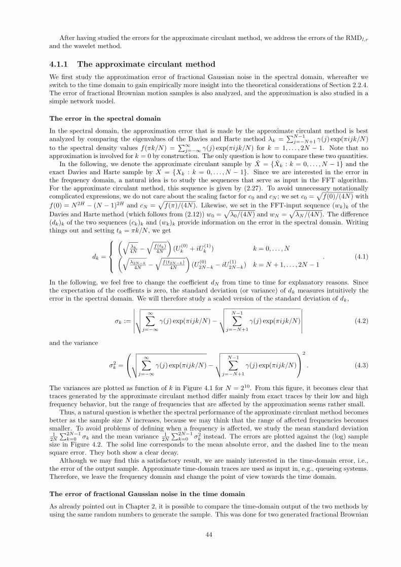
After having studied the errors for the approximate circulant method, we address the errors of the RMDl,r
and the wavelet method.
4.1.1 The approximate circulant method
We first study the approximation error of fractional Gaussian noise in the spectral domain, whereafter weswitch to the time domain to gain empirically more insight into the theoretical considerations of Section 2.2.4.The error of fractional Brownian motion samples is also analyzed, and the approximation is also studied in asimple network model.
The error in the spectral domain
In the spectral domain, the approximation error that is made by the approximate circulant method is bestanalyzed by comparing the eigenvalues of the Davies and Harte method λk =
∑N−1j=−N+1 γ(j) exp(πijk/N)
to the spectral density values f(πk/N) =∑∞
j=−∞ γ(j) exp(πijk/N) for k = 1, . . . , 2N − 1. Note that noapproximation is involved for k = 0 by construction. The only question is how to compare these two quantities.
In the following, we denote the approximate circulant sample by X = Xk : k = 0, . . . , N − 1 and theexact Davies and Harte sample by X = Xk : k = 0, . . . , N − 1. Since we are interested in the error inthe frequency domain, a natural idea is to study the sequences that serve as input in the FFT algorithm.For the approximate circulant method, this sequence is given by (2.27). To avoid unnecessary notationallycomplicated expressions, we do not care about the scaling factor for c0 and cN ; we set c0 =
√
f(0)/(4N) with
f(0) = N2H − (N − 1)2H and cN =√
f(π)/(4N). Likewise, we set in the FFT-input sequence (wk)k of the
Davies and Harte method (which follows from (2.12)) w0 =√
λ0/(4N) and wN =√
λN/(4N). The difference(dk)k of the two sequences (ck)k and (wk)k provide information on the error in the spectral domain. Writingthings out and setting tk = πk/N , we get
dk =
(
√
λk
4N −√
f(tk)4N
)
(U(0)k + iU
(1)k ) k = 0, . . . , N
(
√
λ2N−k
4N −√
f(t2N−k)4N
)
(U(0)2N−k − iU
(1)2N−k) k = N + 1, . . . , 2N − 1
. (4.1)
In the following, we feel free to change the coefficient dN from time to time for explanatory reasons. Sincethe expectation of the coeffients is zero, the standard deviation (or variance) of dk measures intuitively theerror in the spectral domain. We will therefore study a scaled version of the standard deviation of dk,
σk :=
∣
∣
∣
∣
∣
∣
√
√
√
√
∞∑
j=−∞
γ(j) exp(πijk/N) −
√
√
√
√
N−1∑
j=−N+1
γ(j) exp(πijk/N)
∣
∣
∣
∣
∣
∣
(4.2)
and the variance
σ2k =
√
√
√
√
∞∑
j=−∞
γ(j) exp(πijk/N) −
√
√
√
√
N−1∑
j=−N+1
γ(j) exp(πijk/N)
2
. (4.3)
The variances are plotted as function of k in Figure 4.1 for N = 210. From this figure, it becomes clear thattraces generated by the approximate circulant method differ mainly from exact traces by their low and highfrequency behavior, but the range of frequencies that are affected by the approximation seems rather small.
Thus, a natural question is whether the spectral performance of the approximate circulant method becomesbetter as the sample size N increases, because we may think that the range of affected frequencies becomessmaller. To avoid problems of defining when a frequency is affected, we study the mean standard deviation1
2N
∑2N−1k=0 σk and the mean variance 1
2N
∑2N−1k=0 σ2
k instead. The errors are plotted against the (log) samplesize in Figure 4.2. The solid line corresponds to the mean absolute error, and the dashed line to the meansquare error. They both show a clear decay.
Although we may find this a satisfactory result, we are mainly interested in the time-domain error, i.e.,the error of the output sample. Approximate time-domain traces are used as input in, e.g., queueing systems.Therefore, we leave the frequency domain and change the point of view towards the time domain.
The error of fractional Gaussian noise in the time domain
As already pointed out in Chapter 2, it is possible to compare the time-domain output of the two methods byusing the same random numbers to generate the sample. This was done for two generated fractional Brownian
44
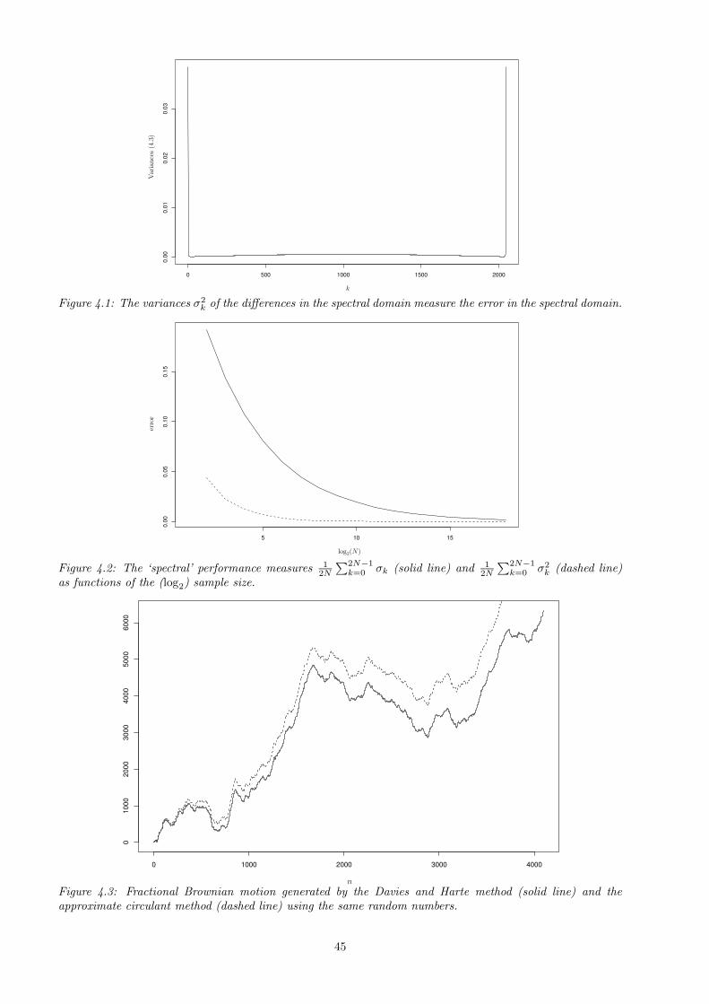
0 500 1000 1500 2000
0.00
0.01
0.02
0.03
PSfrag
replacem
ents
log2 (N
)n
k
Var
iance
s(4
.3)
Figure 4.1: The variances σ2k of the differences in the spectral domain measure the error in the spectral domain.
5 10 15
0.00
0.05
0.10
0.15
PSfrag
replacem
ents
log2(N)nk
erro
r
Figure 4.2: The ‘spectral’ performance measures 12N
∑2N−1k=0 σk (solid line) and 1
2N
∑2N−1k=0 σ2
k (dashed line)as functions of the (log2) sample size.
0 1000 2000 3000 4000
010
0020
0030
0040
0050
0060
00
PSfrag
replacem
ents
log2 (N
)
n
k
Figure 4.3: Fractional Brownian motion generated by the Davies and Harte method (solid line) and theapproximate circulant method (dashed line) using the same random numbers.
45
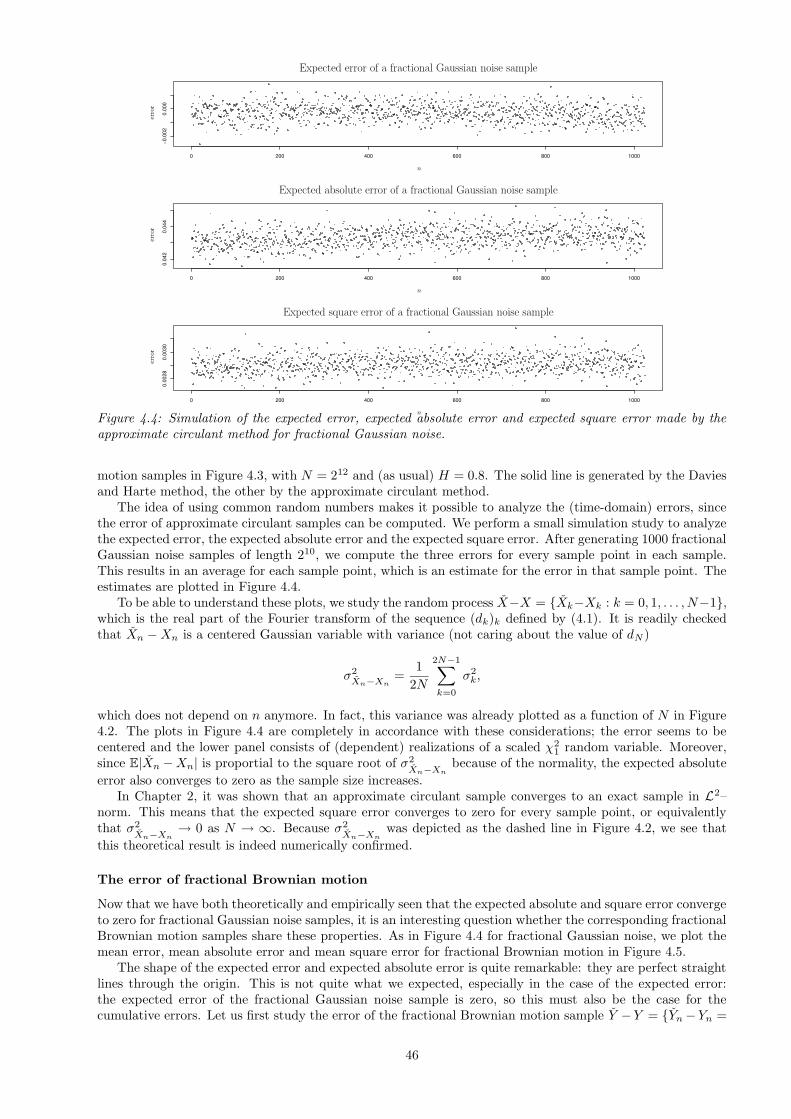
0 200 400 600 800 1000−0
.002
0.00
0
0 200 400 600 800 1000
0.04
20.
044
0 200 400 600 800 1000
0.00
280.
0030
PSfrag
replacem
ents
log2 (N
)nk
Expected error of a fractional Gaussian noise sample
Expected absolute error of a fractional Gaussian noise sample
Expected square error of a fractional Gaussian noise sample
erro
rer
ror
erro
r
n
n
n
Figure 4.4: Simulation of the expected error, expected absolute error and expected square error made by theapproximate circulant method for fractional Gaussian noise.
motion samples in Figure 4.3, with N = 212 and (as usual) H = 0.8. The solid line is generated by the Daviesand Harte method, the other by the approximate circulant method.
The idea of using common random numbers makes it possible to analyze the (time-domain) errors, sincethe error of approximate circulant samples can be computed. We perform a small simulation study to analyzethe expected error, the expected absolute error and the expected square error. After generating 1000 fractionalGaussian noise samples of length 210, we compute the three errors for every sample point in each sample.This results in an average for each sample point, which is an estimate for the error in that sample point. Theestimates are plotted in Figure 4.4.
To be able to understand these plots, we study the random process X−X = Xk−Xk : k = 0, 1, . . . , N−1,which is the real part of the Fourier transform of the sequence (dk)k defined by (4.1). It is readily checkedthat Xn −Xn is a centered Gaussian variable with variance (not caring about the value of dN )
σ2Xn−Xn
=1
2N
2N−1∑
k=0
σ2k,
which does not depend on n anymore. In fact, this variance was already plotted as a function of N in Figure4.2. The plots in Figure 4.4 are completely in accordance with these considerations; the error seems to becentered and the lower panel consists of (dependent) realizations of a scaled χ2
1 random variable. Moreover,since E|Xn −Xn| is proportial to the square root of σ2
Xn−Xnbecause of the normality, the expected absolute
error also converges to zero as the sample size increases.In Chapter 2, it was shown that an approximate circulant sample converges to an exact sample in L2–
norm. This means that the expected square error converges to zero for every sample point, or equivalentlythat σ2
Xn−Xn→ 0 as N → ∞. Because σ2
Xn−Xnwas depicted as the dashed line in Figure 4.2, we see that
this theoretical result is indeed numerically confirmed.
The error of fractional Brownian motion
Now that we have both theoretically and empirically seen that the expected absolute and square error convergeto zero for fractional Gaussian noise samples, it is an interesting question whether the corresponding fractionalBrownian motion samples share these properties. As in Figure 4.4 for fractional Gaussian noise, we plot themean error, mean absolute error and mean square error for fractional Brownian motion in Figure 4.5.
The shape of the expected error and expected absolute error is quite remarkable: they are perfect straightlines through the origin. This is not quite what we expected, especially in the case of the expected error:the expected error of the fractional Gaussian noise sample is zero, so this must also be the case for thecumulative errors. Let us first study the error of the fractional Brownian motion sample Y −Y = Yn −Yn =
46
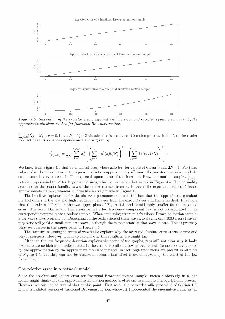
0 200 400 600 800 1000
0.0
0.5
1.0
1.5
2.0
2.5
0 200 400 600 800 1000
010
2030
40
0 200 400 600 800 1000
050
015
0025
00
PSfrag
replacem
ents
log2 (N
)nk
Expected error of a fractional Brownian motion sample
Expected absolute error of a fractional Brownian motion sample
Expected square error of a fractional Brownian motion sample
erro
rer
ror
erro
r
n
n
n
Figure 4.5: Simulation of the expected error, expected absolute error and expected square error made by theapproximate circulant method for fractional Brownian motion.
∑nj=0(Xj −Xj) : n = 0, 1, . . . , N − 1. Obviously, this is a centered Gaussian process. It is left to the reader
to check that its variance depends on n and is given by
σ2Yn−Yn
=1
2N
2N−1∑
k=0
σ2k
n∑
j=0
cos2(πjk/N)
2
+
n∑
j=0
sin2(πjk/N)
2
.
We know from Figure 4.1 that σ2k is almost everywhere zero but for values of k near 0 and 2N − 1. For these
values of k, the term between the square brackets is approximately n2, since the sine-term vanishes and thecosine-term is very close to 1. The expected square error of the fractional Brownian motion sample σ2
Yn−Yn
is thus proportional to n2 for large sample sizes, which is precisely what we see in Figure 4.5. The normalityaccounts for the proportionality to n of the expected absolute error. However, the expected error itself shouldapproximately be zero, whereas it looks like a straight line in Figure 4.5.
The intuitive explanation for the observed phenomenon lies in the fact that the approximate circulantmethod differs in the low and high frequency behavior from the exact Davies and Harte method. First notethat the scale is different in the two upper plots of Figure 4.5, and considerably smaller for the expectederror. The exact Davies and Harte sample has a low frequency component that is not incorporated in thecorresponding approximate circulant sample. When simulating errors in a fractional Brownian motion sample,a big wave shows typically up. Depending on the realizations of these waves, averaging only 1000 errors (waves)may very well yield a small ‘non-zero wave’, although the ‘expectation’ of that wave is zero. This is preciselywhat we observe in the upper panel of Figure 4.5.
The intuitive reasoning in terms of waves also explains why the averaged absolute error starts at zero andwhy it increases. However, it fails to explain why this results in a straight line.
Although the low frequency deviation explains the shape of the graphs, it is still not clear why it lookslike there are no high frequencies present in the errors. Recall that low as well as high frequencies are affectedby the approximation by the approximate circulant method. In fact, high frequencies are present in all plotsof Figure 4.5, but they can not be observed, because this effect is overshadowed by the effect of the lowfrequencies.
The relative error in a network model
Since the absolute and square error for fractional Brownian motion samples increase obviously in n, thereader might think that this approximate simulation method is of no use to simulate a network traffic process.However, we can not be sure of that at this point. First recall the network traffic process A of Section 1.3.It is a translated version of fractional Brownian motion, where A(t) represented the cumulative traffic in the
47
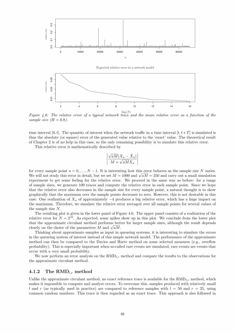
0 10000 20000 30000 40000 50000 600000.
00.
10.
20.
3
2 4 6 8 10 12 14 16
0.01
0.03
0.05
PSfrag
replacem
ents
log2(N)
n
k
rela
tive
erro
rre
lati
veer
ror
Expected relative error in a network model
Figure 4.6: The relative error of a typical network trace and the mean relative error as a function of thesample size (H = 0.8).
time interval [0, t]. The quantity of interest when the network traffic in a time interval [t, t+T ] is simulated isthus the absolute (or square) error of the generated value relative to the ‘exact’ value. The theoretical resultof Chapter 2 is of no help in this case, so the only remaining possibility is to simulate this relative error.
This relative error is mathematically described by
∣
∣
∣
∣
∣
√aM(Xn − Xn)
M +√aMXn
∣
∣
∣
∣
∣
for every sample point n = 0, . . . , N − 1. It is interesting how this error behaves as the sample size N varies.We will not study this error in detail, but we set M = 1000 and
√aM = 250 and carry out a small simulation
experiment to get some feeling for the relative error. We proceed in the same way as before: for a rangeof sample sizes, we generate 100 traces and compute the relative error in each sample point. Since we hopethat the relative error also decreases in the sample size for every sample point, a natural thought is to showgraphically that the maximum over the sample points decreases to zero. However, this is not desirable in thiscase. One realization of Xn of approximately −4 produces a big relative error, which has a huge impact onthe maximum. Therefore, we simulate the relative error averaged over all sample points for several values ofthe sample size N .
The resulting plot is given in the lower panel of Figure 4.6. The upper panel consists of a realization of therelative error for N = 216. As expected, some spikes show up in this plot. We conclude from the lower plotthat the approximate circulant method performs better for larger sample sizes, although the result dependsclearly on the choice of the parameters M and
√aM .
Thinking about approximate samples as input in queueing systems, it is interesting to simulate the errorsin the queueing system of interest instead of this simple network model. The performance of the approximatemethod can then be compared to the Davies and Harte method on some selected measures (e.g., overflowprobability). This is especially important when so-called rare events are simulated; rare events are events thatoccur with a very small probability.
We now perform an error analysis on the RMDl,r method and compare the results to the observations forthe approximate circulant method.
4.1.2 The RMDl,r method
Unlike the approximate circulant method, no exact reference trace is available for the RMDl,r method, whichmakes it impossible to compute and analyze errors. To overcome this, samples produced with relatively smalll and r (as typically used in practice) are compared to reference samples with l = 50 and r = 25, usingcommon random numbers. This trace is then regarded as an exact trace. This approach is also followed in
48
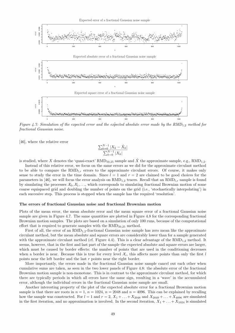
0 200 400 600 800 1000
−0.0
040.
002
0.00
6
0 200 400 600 800 1000
0.01
00.
020
0.03
0
0 200 400 600 800 1000
0.00
050.
0015
PSfrag
replacem
ents
log2 (N
)nk
Expected error of a fractional Gaussian noise sample
Expected absolute error of a fractional Gaussian noise sample
Expected square error of a fractional Gaussian noise sample
erro
rer
ror
erro
r
n
n
n
Figure 4.7: Simulation of the expected error and the expected absolute error made by the RMD1,2 method forfractional Gaussian noise.
[46], where the relative error∑N−1
k=0 |Xk − Xk|∑N−1
k=0 |Xk|
is studied, where X denotes the ‘quasi-exact’ RMD50,25 sample and X the approximate sample, e.g., RMD1,2.Instead of this relative error, we focus on the same errors as we did for the approximate circulant method
to be able to compare the RMDl,r errors to the approximate circulant errors. Of course, it makes onlysense to study the error in the time domain. Since l = 1 and r = 2 are claimed to be good choices for theparameters in [46], we will focus the error analysis on RMD1,2 traces. Recall that an RMDl,r sample is foundby simulating the processes X0,X1, . . ., which corresponds to simulating fractional Brownian motion of somecoarse equispaced grid and doubling the number of points on the grid (i.e., ‘stochastically interpolating’) ineach succesive step. This process is stopped when the sample has the required ‘resolution’.
The errors of fractional Gaussian noise and fractional Brownian motion
Plots of the mean error, the mean absolute error and the mean square error of a fractional Gaussian noisesample are given in Figure 4.7. The same quantities are plotted in Figure 4.8 for the corresponding fractionalBrownian motion samples. The plots are based on a simulation of only 100 runs, because of the computationaleffort that is required to generate samples with the RMD50,25 method.
First of all, the error of an RMD1,2-fractional Gaussian noise sample has zero mean like the approximatecirculant method, but the mean absolute and square errors are considerably lower than for a sample generatedwith the approximate circulant method (cf. Figure 4.4). This is a clear advantage of the RMD1,2 method. Itseems, however, that in the first and last part of the sample the expected absolute and square errors are larger,which must be caused by border effects: the number of points that are used in the conditioning decreaseswhen a border is near. Because this is true for every level Xi, this affects more points than only the first lpoints near the left border and the last r points near the right border.
More importantly, the errors made in the fractional Gaussian noise sample cancel out each other whencumulative sums are taken, as seen in the two lower panels of Figure 4.8: the absolute error of the fractionalBrownian motion sample is non-monotone. This is in contrast to the approximate circulant method, for whichthere are typically periods in which all errors have the same sign, resulting in a ‘wave’ in the accumulatederror, although the individual errors in the fractional Gaussian noise sample are small.
Another interesting property of the plot of the expected absolute error for a fractional Brownian motionsample is that there are roots in n = 1, n = 1024, n = 2048 and n = 4096. This can be explained by recallinghow the sample was constructed. For l = 1 and r = 2, X1 + . . .+X2048 and X2049 + . . .+X4096 are simulatedin the first iteration, and no approximation is involved. In the second iteration, X1 + . . .+X1024 is simulated
49
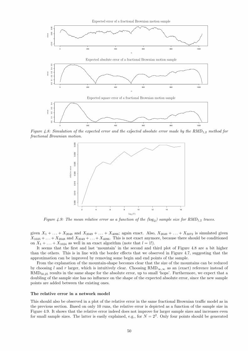
0 200 400 600 800 1000−0
.10
0.00
0.05
0 200 400 600 800 1000
0.0
0.1
0.2
0.3
0.4
0.5
0 200 400 600 800 1000
0.0
0.1
0.2
0.3
0.4
PSfrag
replacem
ents
log2 (N
)nk
Expected error of a fractional Brownian motion sample
Expected absolute error of a fractional Brownian motion sample
Expected square error of a fractional Brownian motion sample
erro
rer
ror
erro
r
n
n
n
Figure 4.8: Simulation of the expected error and the expected absolute error made by the RMD1,2 method forfractional Brownian motion.
2 4 6 8 10 12 14 16
0.00
50.
010
0.01
50.
020
0.02
50.
030
0.03
5
PSfrag
replacem
ents
log2(N)
nk
rela
tive
erro
r
Figure 4.9: The mean relative error as a function of the (log2) sample size for RMD1,2 traces.
given X1 + . . . + X2048 and X2049 + . . . + X4096; again exact. Also, X2049 + . . . + X3072 is simulated givenX1025 + . . .+X2048 and X2049 + . . .+X4096. This is not exact anymore, because there should be conditionedon X1 + . . .+X1024 as well in an exact algorithm (note that l = 1!).
It seems that the first and last ‘mountain’ in the second and third plot of Figure 4.8 are a bit higherthan the others. This is in line with the border effects that we observed in Figure 4.7, suggesting that theapproximation can be improved by removing some begin and end points of the sample.
From the explanation of the mountain-shape becomes clear that the size of the mountains can be reducedby choosing l and r larger, which is intuitively clear. Choosing RMD∞,∞ as an (exact) reference instead ofRMD50,25 results in the same shape for the absolute error, up to small ‘hops’. Furthermore, we expect that adoubling of the sample size has no influence on the shape of the expected absolute error, since the new samplepoints are added between the existing ones.
The relative error in a network model
This should also be observed in a plot of the relative error in the same fractional Brownian traffic model as inthe previous section. Based on only 10 runs, the relative error is depicted as a function of the sample size inFigure 4.9. It shows that the relative error indeed does not improve for larger sample sizes and increases evenfor small sample sizes. The latter is easily explained, e.g., for N = 22. Only four points should be generated
50
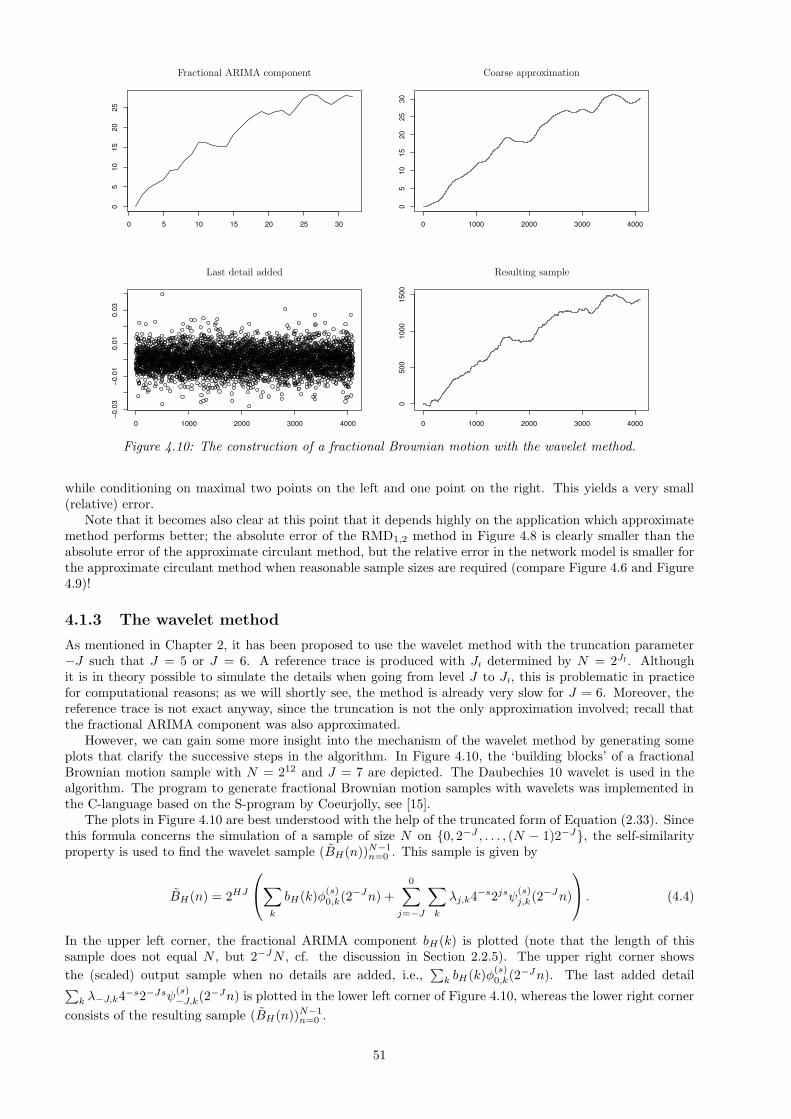
0 5 10 15 20 25 30
05
1015
2025
0 1000 2000 3000 4000
05
1015
2025
30
0 1000 2000 3000 4000
−0.0
3−0
.01
0.01
0.03
0 1000 2000 3000 4000
050
010
0015
00
PSfrag
replacem
ents
log2 (N
)nk
Fractional ARIMA component Coarse approximation
Last detail added Resulting sample
Figure 4.10: The construction of a fractional Brownian motion with the wavelet method.
while conditioning on maximal two points on the left and one point on the right. This yields a very small(relative) error.
Note that it becomes also clear at this point that it depends highly on the application which approximatemethod performs better; the absolute error of the RMD1,2 method in Figure 4.8 is clearly smaller than theabsolute error of the approximate circulant method, but the relative error in the network model is smaller forthe approximate circulant method when reasonable sample sizes are required (compare Figure 4.6 and Figure4.9)!
4.1.3 The wavelet method
As mentioned in Chapter 2, it has been proposed to use the wavelet method with the truncation parameter−J such that J = 5 or J = 6. A reference trace is produced with Jf determined by N = 2Jf . Althoughit is in theory possible to simulate the details when going from level J to Jf, this is problematic in practicefor computational reasons; as we will shortly see, the method is already very slow for J = 6. Moreover, thereference trace is not exact anyway, since the truncation is not the only approximation involved; recall thatthe fractional ARIMA component was also approximated.
However, we can gain some more insight into the mechanism of the wavelet method by generating someplots that clarify the successive steps in the algorithm. In Figure 4.10, the ‘building blocks’ of a fractionalBrownian motion sample with N = 212 and J = 7 are depicted. The Daubechies 10 wavelet is used in thealgorithm. The program to generate fractional Brownian motion samples with wavelets was implemented inthe C-language based on the S-program by Coeurjolly, see [15].
The plots in Figure 4.10 are best understood with the help of the truncated form of Equation (2.33). Sincethis formula concerns the simulation of a sample of size N on 0, 2−J , . . . , (N − 1)2−J, the self-similarityproperty is used to find the wavelet sample (BH(n))N−1
n=0 . This sample is given by
BH(n) = 2HJ
∑
k
bH(k)φ(s)0,k(2−Jn) +
0∑
j=−J
∑
k
λj,k4−s2jsψ(s)j,k(2−Jn)
. (4.4)
In the upper left corner, the fractional ARIMA component bH(k) is plotted (note that the length of thissample does not equal N , but 2−JN , cf. the discussion in Section 2.2.5). The upper right corner shows
the (scaled) output sample when no details are added, i.e.,∑
k bH(k)φ(s)0,k(2−Jn). The last added detail
∑
k λ−J,k4−s2−Jsψ(s)−J,k(2−Jn) is plotted in the lower left corner of Figure 4.10, whereas the lower right corner
consists of the resulting sample (BH(n))N−1n=0 .
51
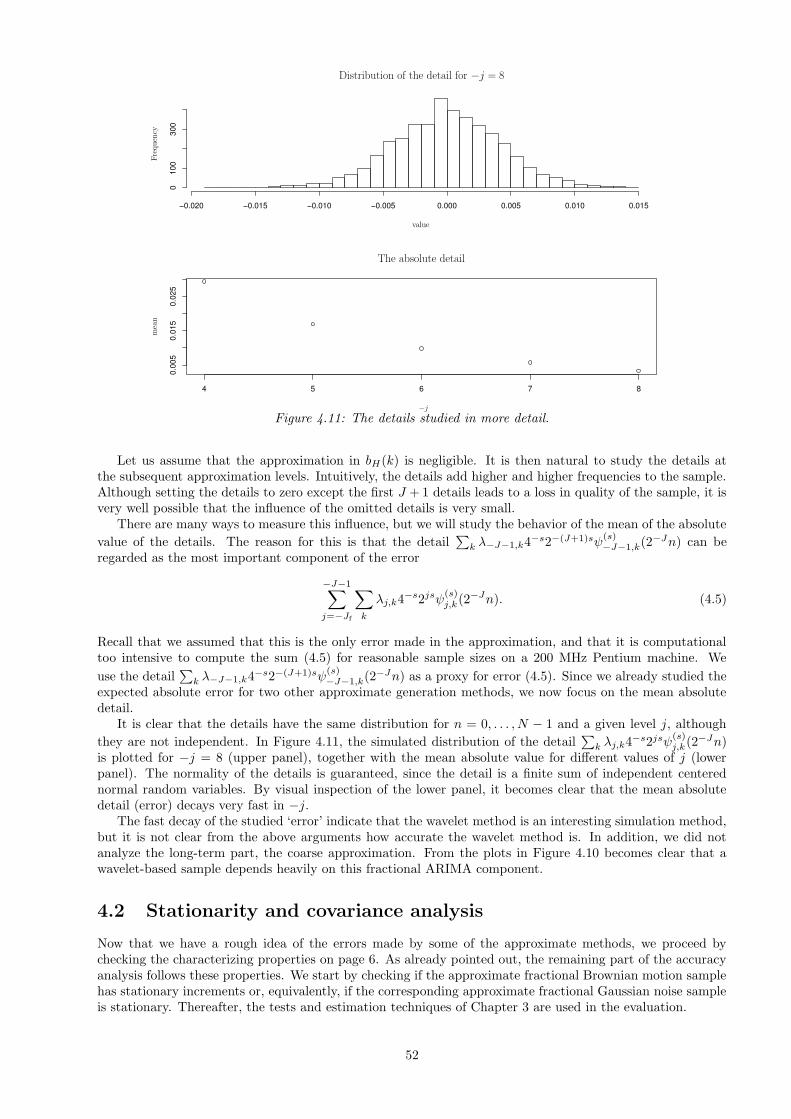
−0.020 −0.015 −0.010 −0.005 0.000 0.005 0.010 0.015
010
030
0
4 5 6 7 8
0.00
50.
015
0.02
5
PSfrag
replacem
ents
log2 (N
)nk
Distribution of the detail for −j = 8
The absolute detail
−j
value
Fre
quen
cym
ean
Figure 4.11: The details studied in more detail.
Let us assume that the approximation in bH(k) is negligible. It is then natural to study the details atthe subsequent approximation levels. Intuitively, the details add higher and higher frequencies to the sample.Although setting the details to zero except the first J + 1 details leads to a loss in quality of the sample, it isvery well possible that the influence of the omitted details is very small.
There are many ways to measure this influence, but we will study the behavior of the mean of the absolute
value of the details. The reason for this is that the detail∑
k λ−J−1,k4−s2−(J+1)sψ(s)−J−1,k(2−Jn) can be
regarded as the most important component of the error
−J−1∑
j=−Jf
∑
k
λj,k4−s2jsψ(s)j,k(2−Jn). (4.5)
Recall that we assumed that this is the only error made in the approximation, and that it is computationaltoo intensive to compute the sum (4.5) for reasonable sample sizes on a 200 MHz Pentium machine. We
use the detail∑
k λ−J−1,k4−s2−(J+1)sψ(s)−J−1,k(2−Jn) as a proxy for error (4.5). Since we already studied the
expected absolute error for two other approximate generation methods, we now focus on the mean absolutedetail.
It is clear that the details have the same distribution for n = 0, . . . , N − 1 and a given level j, although
they are not independent. In Figure 4.11, the simulated distribution of the detail∑
k λj,k4−s2jsψ(s)j,k(2−Jn)
is plotted for −j = 8 (upper panel), together with the mean absolute value for different values of j (lowerpanel). The normality of the details is guaranteed, since the detail is a finite sum of independent centerednormal random variables. By visual inspection of the lower panel, it becomes clear that the mean absolutedetail (error) decays very fast in −j.
The fast decay of the studied ‘error’ indicate that the wavelet method is an interesting simulation method,but it is not clear from the above arguments how accurate the wavelet method is. In addition, we did notanalyze the long-term part, the coarse approximation. From the plots in Figure 4.10 becomes clear that awavelet-based sample depends heavily on this fractional ARIMA component.
4.2 Stationarity and covariance analysis
Now that we have a rough idea of the errors made by some of the approximate methods, we proceed bychecking the characterizing properties on page 6. As already pointed out, the remaining part of the accuracyanalysis follows these properties. We start by checking if the approximate fractional Brownian motion samplehas stationary increments or, equivalently, if the corresponding approximate fractional Gaussian noise sampleis stationary. Thereafter, the tests and estimation techniques of Chapter 3 are used in the evaluation.
52
It is in general extremely difficult to show statistically that a sample is stationary (more precisely: that asample is a realization of a stationary process). Many tests are only suitable in certain cases. In addition, muchliterature on tests for stationarity deal with testing if one particular sample can be regarded as stationary,assuming a specific form of the underlying stochastic process. In the presence of long-range dependence, it iseven more difficult to distinguish a stationary process with long memory from a non-stationary process; thereappear to be local trends and cycles, which are spurious and disappear after some time [9]. In our situation,we can simulate as many samples as we like, which may be exploited in the stationarity check.
Instead of testing the stationarity statistically, we investigate theoretically whether an approximate methodproduces stationary samples.
Spectral methods
An example of a method for which it is possible to show that stationary samples are produced is the spectralsimulation method (see Section 2.2.4).
Although the spectral simulation method, the Paxson, and approximate circulant method are closelyrelated, we cannot conclude from this fact that Paxson and approximate circulant samples are also stationary.Whereas we could afford some sloppiness with respect to some input FFT-coeffients in the error analysis, itis possible that these coefficients distort the stationarity.
Fortunately, this is not the case. Direct computations for the Paxson method using (2.25) show that forPaxson samples holds that
Cov(Xm, Xn) =
N/2−1∑
k=1
f(2πk/N)
N/2cos(2π(m− n)k/N) +
f(π)
2N(−1)m+n, (4.6)
which depends only on m − n, since (−1)m+n = (−1)m−n. We write γP(·) for the resulting autocovariancefunction. Similar computations for the approximate circulant method show that
Cov(Xm, Xn) =
N−1∑
k=1
f(πk/N)
Ncos(π(m− n)k/N) +
N2H − (N − 1)2H
2N+f(π)
2N(−1)m−n. (4.7)
From this expression it becomes clear that approximate circulant samples are stationary as well. The resultingautocovariance function is denoted by γAC(·).
Some problems arise for the Paxson method at this point. Recall that in a sample of size N , the covariancesγ(0), . . . , γ(N − 1) are approximated by γP(0), . . . , γP(N − 1). From (1.7) follows that the autocovariancefunction γ(k) decreases in k for H > 1/2, but this is not the case for the approximation γP(k), since thisfunction is symmetrical around k = N/2.
To illustrate this problem, the autocovariance function γP is plotted together with the autocovariancefunction γ for H = 0.8 and N = 28 in the upper panel of Figure 4.12. The lower panel consists of thefunctions γAC and γ.
Besides the symmetry problem of γP, the differences with the exact autocovariance function are relativelylarge; even negative covariances are present in Paxson samples. Still, the Paxson method passed many checks(see Paxson [47]), even without the normality improvement of Chapter 2. This shows how much care should betaken in the evaluation of approximate simulation methods! It should be said that γP approximates γ betteras the sample size N increases, which is probably the reason for Paxson’s empirical finding that satisfactorysamples are obtained for N = 215.
The autocovariance function γAC of the approximate circulant method is more promising, indicated bythe plot in the lower panel of Figure 4.12. Except for high-lag autocovariances, the function is almostindistinguishable from γ, which even improves for N → ∞. In fact, from Equation (4.6) and (4.7) it becomesclear that γP as well as γAC converge to γ as N → ∞ (compare (2.22)):
γP/AC(k) → 2
∫ π
0
f(λ)
2πcos(kλ)dλ = γ(k).
However, we are particularly interested in the rate of convergence to zero of γAC, which cannot be observedin this plot1. For a long-range dependent process with Hurst parameter H = 0.8, the graph of γ on a log-logscale is a straight line with slope 2H − 2 = −0.4 for large k.
To check if this is the case for the autocovariance function of the approximate circulant method withH = 0.8, the log-log plot is given in Figure 4.13 for N = 211 and N = 213. Since we are only interested in thetail behavior, the plot of the autocovariance function starts with k = 210.
1I am grateful to Marius Ooms for pointing this out to me.
53
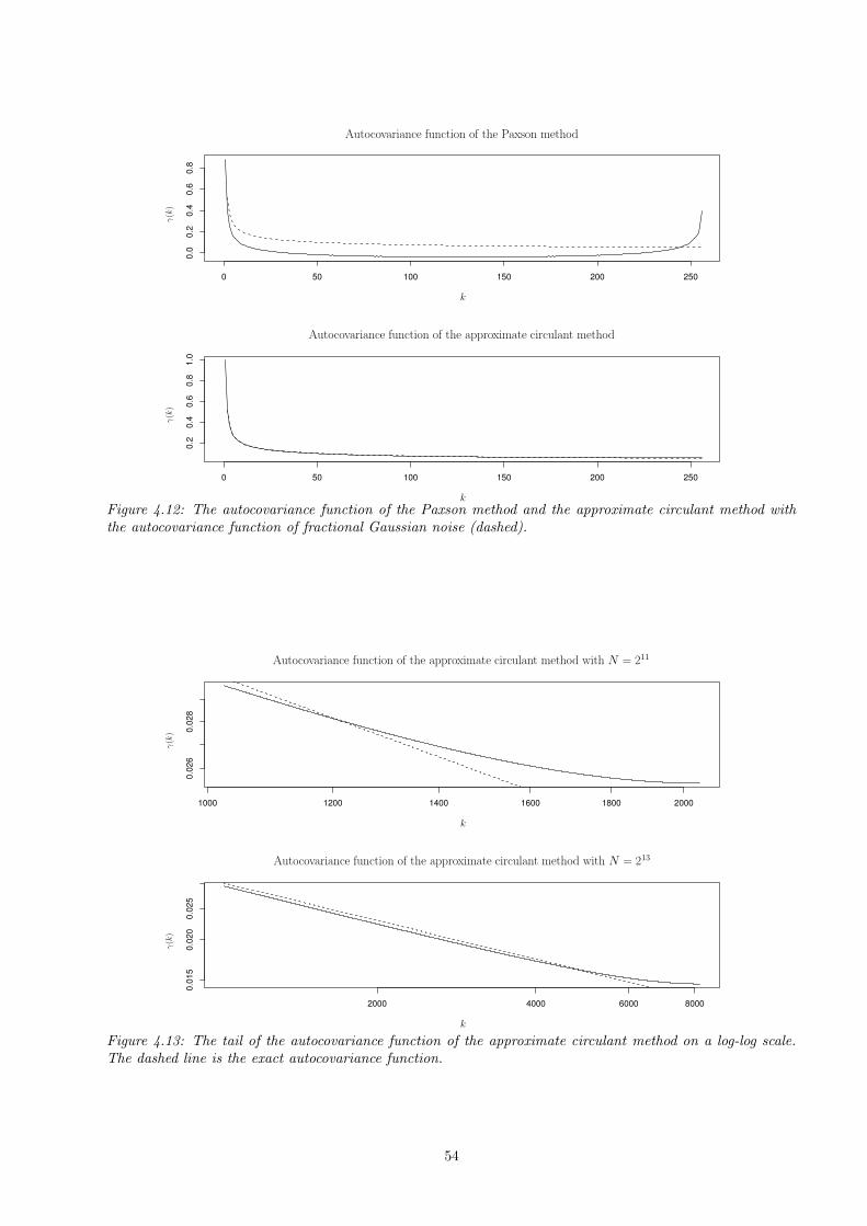
0 50 100 150 200 250
0.0
0.2
0.4
0.6
0.8
0 50 100 150 200 250
0.2
0.4
0.6
0.8
1.0
PSfrag
replacem
ents
log2 (N
)nk
Autocovariance function of the Paxson method
Autocovariance function of the approximate circulant method
γ(k
)γ(k
)
k
k
Figure 4.12: The autocovariance function of the Paxson method and the approximate circulant method withthe autocovariance function of fractional Gaussian noise (dashed).
1000 1200 1400 1600 1800 2000
0.02
60.
028
2000 4000 6000 8000
0.01
50.
020
0.02
5
PSfrag
replacem
ents
log2 (N
)nkAutocovariance function of the approximate circulant method with N = 211
Autocovariance function of the approximate circulant method with N = 213
γ(k
)γ(k
)
k
k
Figure 4.13: The tail of the autocovariance function of the approximate circulant method on a log-log scale.The dashed line is the exact autocovariance function.
54
We see that the exact autocovariance function is indeed a straight line, but that this is not the case for theautocovariance function of the approximate circulant method. The differences at the left end of the graph arequite small, and can presumably even be made smaller by implementing one of the suggested improvementsof Section 2.2.4. It is more interesting that the solid line curves upwards for the approximate circulantmethod. Because the graph was depicted on a log-log scale, this involves many high-lag autocovariances.From these plots it becomes indeed plausible that the autocovariance function converges pointwise to theexact autocovariance function, although in each case approximately half of the autocovariances is badlyapproximated. If a sample of size N is needed, an obvious improvement is thus to take the first N elementsof an approximate circulant sample of size 2N . This also makes the method twice as slow.
The RMDl,r method
It is not always possible to find an explicit expression for the covariance function. For instance, it is notclear how the covariances of the wavelet method can be computed. Norros et al. [46] make a plot of thecovariance matrices of the RMD0,1 and RMD1,1 method. From this becomes clear that the RMDl,r methodapproximates the covariance matrix by a non-stationary ‘terrace architecture’. However, it is not discussed in[46] how to compute the covariance matrix of the RMDl,r method for general l ≥ 0 and r ≥ 1. We will nowdescribe how this covariance matrix can numerically be found. Since the same techniques are used as in thegeneration method, we will only discuss the main idea in a small example.
Recall that Xi = Xij = BH(j2−i) − BH((j − 1)2−i) : j = 1, . . . , 2i. Consider the probability densityfX2,1,X2,2,X2,3,X2,4
of the random vector (X2,1, X2,2, X2,3, X2,4). This density can be computed by noting that(assume that l ≥ 1 and r ≥ 2)
fX2,1,X2,2,X2,3,X2,4(x1, x2, x3, x4) = fX2,1,X2,1+X2,2,X2,3,X2,3+X2,4
(x1, x1 + x2, x3, x3 + x4)
= fX2,1,X2,3|X2,1+X2,2=x1+x2,X2,3+X2,4=x3+x4(x1, x3)fX2,1+X2,2,X2,3+X2,4
(x1 + x2, x3 + x4)
= fX2,1,X2,3|X1,1=x1+x2,X1,2=x3+x4(x1, x3)fX1,1,X1,2
(x1 + x2, x3 + x4)
= fX2,1|X1,1=x1+x2,X1,2=x3+x4(x1)fX2,3|X2,1=x1,X2,2=x2,X1,2=x3+x4
(x3)
·fX1,1,X1,2(x1 + x2, x3 + x4).
In the notation of Section 2.2.3, it is readily checked that the previous formula implies that
(x1, x2, x3, x4)Γ−12 (x1, x2, x3, x4)
′ =(x1 − e(2, 0)(x1 + x2, x3 + x4)
′)2
v(2, 0)
+(x3 − e(2, 1)(x1, x2, x3 + x4)
′)2
v(2, 1)
+ (x1 + x2, x3 + x4)Γ−11 (x1 + x2, x3 + x4)
′.
From this, the inverse Γ−12 of the covariance matrix of (X2,1, X2,2, X2,3, X2,4) is determined uniquely and
can be computed once the inverse Γ−11 of the covariance matrix of (X1,1, X1,2) is known. This is done by
writing every term on the right hand side in the form (x1, x2, x3, x4)A(x1, x2, x3, x4)′ for some matrix A, thus
rewriting the whole right hand side in this form, which gives the matrix Γ−12 . The same idea can be used
to compute Γ−13 , Γ−1
4 , and so on. The truncation parameters l and r show up when for instance r = 1 andfX2,1|X1,1=x1+x2,X1,2=x3+x4
(x1) is approximated by fX2,1|X1,1=x1+x2(x1).
When the covariance matrix of the RMDl,r method for a sample size N = 2g should be computed, thisprocess is stopped once Γ−1
g is known. The inverse of Γ−1g is then the required covariance matrix.
In Figure 4.14, the covariance matrices of the RMD1,1 and RMD1,2 method are plotted. In the terminologyof [46], the ‘terrace architecture’ is clearly present in the RMD1,1 matrix, whereas it seems to have disappearedin the RMD1,2 matrix. The RMD1,2 matrix is visually almost indistinguishable from the exact covariancematrix. However, the matrices are not equal. As already pointed out, the approximate covariance matrix doesnot correspond to a stationary process. Therefore, it is impossible to analyze the covariances of the RMDl,r
method in the same way as we did for the spectral methods: the diagonal and its parallel vectors do not haveconstant elements anymore. Therefore, we plot the minimum and maximum value of each ‘diagonal’ vector.From this, we can still get an idea about the decay of the elements in the covariance matrix. The resultingplot is given in Figure 4.15 for the RMD1,2 and RMD3,3 methods with sample size N = 28.
Note that no information is provided by Figure 4.15 on the distribution of the ‘diagonal’ vectors; it is wellpossible that all covariances are exact, except for two covariances: the minimum and the maximum value. Infact, the lines that correspond to the first and third quartile of this distribution lie very close to the exactvalue except for the rightmost part (these quartile-lines were not depicted to prevent them from spoiling thevisual effect of the plot). Like the observations in the error analysis, this suggests that these methods are very
55
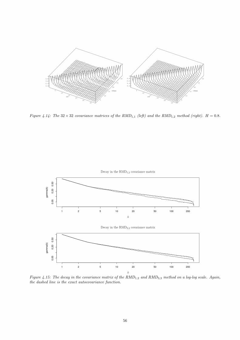
5
10
15
20
25
30
5
10
15
20
25
30
0.2
0.4
0.6
0.8
1
PSfrag
replacem
ents
log2 (N
)nk
row
column 5
10
15
20
25
30
5
10
15
20
25
30
0.2
0.4
0.6
0.8
1
PSfrag
replacem
ents
log2 (N
)nk
row
column
Figure 4.14: The 32× 32 covariance matrices of the RMD1,1 (left) and the RMD1,2 method (right). H = 0.8.
1 2 5 10 20 50 100 200
0.05
0.20
0.50
gam
ma(
k)
1 2 5 10 20 50 100 200
0.05
0.20
0.50
gam
ma(
k)
PSfrag
replacem
ents
log2 (N
)nk Decay in the RMD1,2 covariance matrix
Decay in the RMD3,3 covariance matrix
γ(k
)
k
k
Figure 4.15: The decay in the covariance matrix of the RMD1,2 and RMD3,3 method on a log-log scale. Again,the dashed line is the exact autocovariance function.
56

Davies RMD1,2 RMD2,1 RMD3,3 Paxson approx. wavelet wavelet
& Harte circulant J = 6 J = 7
mean 0.008159 0.008615 0.01958 0.008291 0.1090 0.04486 0.02084 0.02144
max 0.04359 0.05154 0.1961 0.05010 0.3458 0.08606 0.5157 0.3549
Table 4.1: Sample mean and maximum absolute value of the elements in the error matrix.
interesting for simulation purposes. Although the minimum and maximum value of the RMD3,3 method seemsto lie closer to the exact value, the differences between the RMD1,2 and the RMD3,3 method are definitelynot so large. An important observation is that the rightmost part of the graph curves downwards, which isnot desirable. As already suggested in the error analysis, this may be solved by removing some sample pointsat the beginning and the end of the trace.
The wavelet method; a simulation experiment
To gain more insight into the approximation of the covariance structure of the wavelet method, we performa simulation experiment to estimate the covariances. This sample covariance matrix is then compared to thetheoretical covariance matrix determined by the autocovariance function γ(·).
To find a sample covariance matrix, we generate n samples of size N with the wavelet method. Denote
the ith sample by X(i) = X(i)k : k = 0, . . . , N − 1. From these samples, we estimate element (l, k) of the
covariance matrix by
1
n− 1
(
n−1∑
i=0
X(i)l X
(i)k − 1
n
[
n−1∑
i=0
X(i)l
n−1∑
i=0
X(i)k
])
,
for l, k = 0, . . . , N − 1. After that, the theoretical covariance matrix is substracted from the estimated matrixto obtain the ‘sample error’ matrix.
The average absolute value and the largest absolute value of the elements in the error matrix provideinformation on how well the wavelet method performs. To make it possible to compare the wavelet errormatrix, the procedure is also followed for the Davies and Harte method and the other approximate methods.The largest absolute error and the mean absolute error are tabulated in Table 4.1. All samples are of sizeN = 28 and were generated with input Hurst parameter H = 0.8. The number of simulation runs is n = 10000.We see that the performance of the RMD2,1 method is rather disappointing, whereas the RMD1,2 and RMD3,3
methods have estimated covariance matrices quite close to the real covariance matrices, as already suggestedby the previous theoretical covariance analysis. This is especially true for the RMD3,3 method, in which moresample points are used in the conditioning. The resulting (non-stationary) samples have covariances that areeven closer to the required covariances than the (stationary) approximate circulant samples! As expected, theapproximate circulant method performs better than the Paxson method, which is reflected by smaller valuesin Table 4.1. In fact, the ‘max’ value is close to the maximum absolute distance between the two covariancefunctions in the upper panel of Figure 4.12, 0.3456. The two wavelet methods perform quite badly, indicatedby the large values in the table. However, we should keep in mind that the covariance matrix was simulated,which makes it hard to draw robust conclusions.
4.3 Testing the approximate samples
According to the properties on page 6 that outline the structure of this accuracy analysis, we should testif long-range with the right Hurst parameter is present in the approximate samples. However, we will firsttest if the approximate simulation methods produce samples that can be regarded as fractional Gaussiannoise. Because it is an assumption in the Whittle estimation procedure that the sample is fractional Gaussiannoise (see Section 3.1.8), this must be done before the Hurst parameter is estimated. To test this assumptionstatistically, we have the two tests described in Chapter 3 at our disposal.
4.3.1 The goodness-of-fit test for the spectral density
The first is Beran’s goodness-of-fit test for the spectral density, which is especially important since the Whittleestimator is also based on a ‘spectral’ approximation of the likelihood function. Using several approximatemethods, 1000 samples of length N = 213 are generated for H = 0.5, H = 0.65 and H = 0.8. For thesesamples, the test statistic is computed and compared to its theoretical (asymptotic) Gaussian distributionusing the Kolmogorov-Smirnov test. Although no problems will emerge for the exact Davies and Harte
57
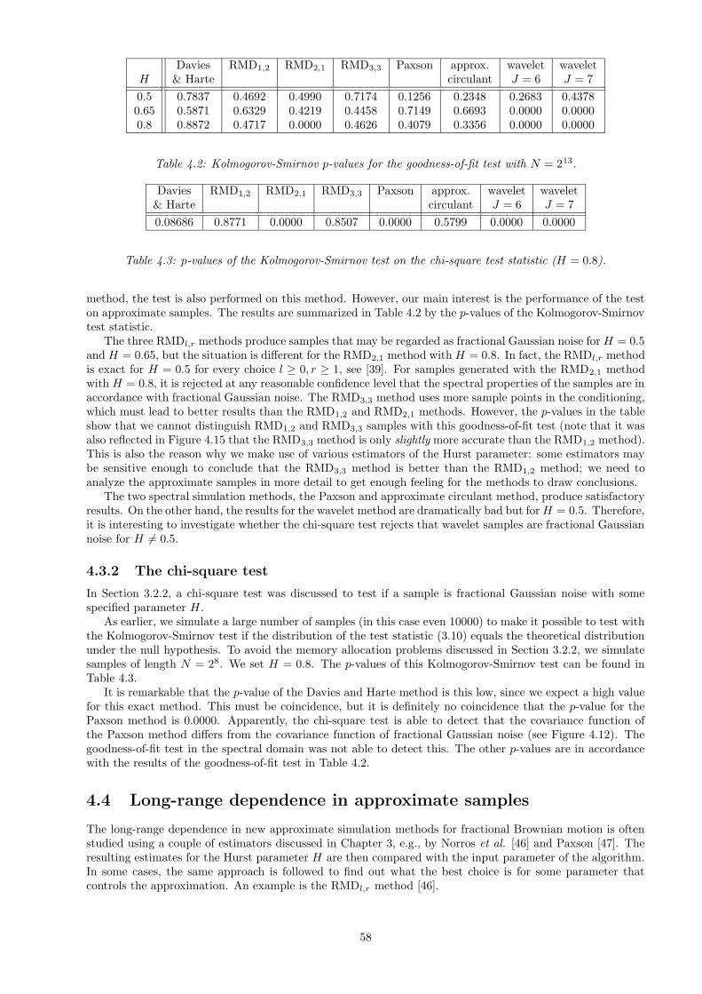
Davies RMD1,2 RMD2,1 RMD3,3 Paxson approx. wavelet waveletH & Harte circulant J = 6 J = 7
0.5 0.7837 0.4692 0.4990 0.7174 0.1256 0.2348 0.2683 0.43780.65 0.5871 0.6329 0.4219 0.4458 0.7149 0.6693 0.0000 0.00000.8 0.8872 0.4717 0.0000 0.4626 0.4079 0.3356 0.0000 0.0000
Table 4.2: Kolmogorov-Smirnov p-values for the goodness-of-fit test with N = 213.
Davies RMD1,2 RMD2,1 RMD3,3 Paxson approx. wavelet wavelet& Harte circulant J = 6 J = 7
0.08686 0.8771 0.0000 0.8507 0.0000 0.5799 0.0000 0.0000
Table 4.3: p-values of the Kolmogorov-Smirnov test on the chi-square test statistic (H = 0.8).
method, the test is also performed on this method. However, our main interest is the performance of the teston approximate samples. The results are summarized in Table 4.2 by the p-values of the Kolmogorov-Smirnovtest statistic.
The three RMDl,r methods produce samples that may be regarded as fractional Gaussian noise for H = 0.5and H = 0.65, but the situation is different for the RMD2,1 method with H = 0.8. In fact, the RMDl,r methodis exact for H = 0.5 for every choice l ≥ 0, r ≥ 1, see [39]. For samples generated with the RMD2,1 methodwith H = 0.8, it is rejected at any reasonable confidence level that the spectral properties of the samples are inaccordance with fractional Gaussian noise. The RMD3,3 method uses more sample points in the conditioning,which must lead to better results than the RMD1,2 and RMD2,1 methods. However, the p-values in the tableshow that we cannot distinguish RMD1,2 and RMD3,3 samples with this goodness-of-fit test (note that it wasalso reflected in Figure 4.15 that the RMD3,3 method is only slightly more accurate than the RMD1,2 method).This is also the reason why we make use of various estimators of the Hurst parameter: some estimators maybe sensitive enough to conclude that the RMD3,3 method is better than the RMD1,2 method; we need toanalyze the approximate samples in more detail to get enough feeling for the methods to draw conclusions.
The two spectral simulation methods, the Paxson and approximate circulant method, produce satisfactoryresults. On the other hand, the results for the wavelet method are dramatically bad but forH = 0.5. Therefore,it is interesting to investigate whether the chi-square test rejects that wavelet samples are fractional Gaussiannoise for H 6= 0.5.
4.3.2 The chi-square test
In Section 3.2.2, a chi-square test was discussed to test if a sample is fractional Gaussian noise with somespecified parameter H.
As earlier, we simulate a large number of samples (in this case even 10000) to make it possible to test withthe Kolmogorov-Smirnov test if the distribution of the test statistic (3.10) equals the theoretical distributionunder the null hypothesis. To avoid the memory allocation problems discussed in Section 3.2.2, we simulatesamples of length N = 28. We set H = 0.8. The p-values of this Kolmogorov-Smirnov test can be found inTable 4.3.
It is remarkable that the p-value of the Davies and Harte method is this low, since we expect a high valuefor this exact method. This must be coincidence, but it is definitely no coincidence that the p-value for thePaxson method is 0.0000. Apparently, the chi-square test is able to detect that the covariance function ofthe Paxson method differs from the covariance function of fractional Gaussian noise (see Figure 4.12). Thegoodness-of-fit test in the spectral domain was not able to detect this. The other p-values are in accordancewith the results of the goodness-of-fit test in Table 4.2.
4.4 Long-range dependence in approximate samples
The long-range dependence in new approximate simulation methods for fractional Brownian motion is oftenstudied using a couple of estimators discussed in Chapter 3, e.g., by Norros et al. [46] and Paxson [47]. Theresulting estimates for the Hurst parameter H are then compared with the input parameter of the algorithm.In some cases, the same approach is followed to find out what the best choice is for some parameter thatcontrols the approximation. An example is the RMDl,r method [46].
58

0.70 0.75 0.80 0.85 0.90
050
100
150
200
PSfrag
replacem
ents
log2 (N
)nk
Fre
quen
cy
H
Figure 4.16: Histogram of the periodogram estimates for exact traces.
Without knowing what the properties of the estimator are, this may lead to wrong conclusions, e.g., whenthe estimator is biased. Assume that the estimator has negative bias; the estimate of the Hurst parameterin exact samples is structural lower than the input parameter H. Let us also assume that we have twoapproximate methods. One produces samples with exact Hurst parameter H, and one the other producessamples with a Hurst parameter H > H. Typically, the estimated Hurst parameter is smaller than H forthe first approximate method. It is possible that the estimate of the Hurst parameter of the second methodequals approximately H. The naive conclusion is then that the second approximate method is better!
It is mostly impossible to study the properties (e.g., bias) of the estimator theoretically. As an example, weconsider the periodogram estimator. If the disturbance term in the linear fitting is a centered Gaussian variablewith equal variance for every sample point and moreover independent, the resulting least-square estimatoris unbiased and normally distributed. However, the distribution of the disturbance term is exponential (seeBeran [9]), so we can not be sure that the estimator is unbiased and Gaussian. The histogram of 1000estimates for the Davies and Harte method is given in Figure 4.16 (H = 0.8, N = 214), and suggests that theestimator is indeed Gaussian, although slightly biased.
In some cases, it is possible to derive a theoretical result concerning the limiting distribution of theestimator. As an example, Coeurjolly [15] uses the asymptotical distribution of his discrete variations estimator(see Section 3.1.3) in his comparison of some approximate simulation methods.
As with all estimators in this section, the parameters of the estimation procedures are chosen as in Chapter3, unless stated otherwise.
To overcome the problem that the distribution of the estimator under the null hypothesis (that the traceshave the right Hurst parameter) is not known, we simply simulate this distribution. After simulating thisdistribution for each approximate simulation method as well, it is tested whether the distributions are equal.In this section, we simulate the distributions of the estimators of Chapter 3 and perform the test of equalityin distribution. This makes it possible to draw conclusions using estimators that are highly biased, whichsolves the earlier mentioned problem.
Several nonparametric tests are available to test the equality of distributions.
Assume we have two populations, X and Y , with cumulative distribution functions denoted by FX andFY , respectively. We have an independent sample of size m drawn from the X population, X1, . . . , Xm andanother independent sample of size n drawn independently from the Y population, Y1, . . . , Yn (note that thism and n have nothing to do with the previously used notation). It is assumed that there are no ties, whichis a reasonable assumption in our case, since we are dealing with continuous distributions. We would like totest the hypothesis that the two samples are drawn from the same distribution, FX(x) = FY (x) for all x.The most general two-sided alternative hypothesis is simply FX(x) 6= FY (x) for some x, but the availabletests under this hypothesis, like the Kolmogorov-Smirnov two-sample test, have little power against smalldeviations in the distribution.
In our case, we expect the differences in the two samples to be rather small, so we should make some
59

concessions and restrict the alternative hypothesis a bit more: we will test against differences in location(mean/median) and scale (interquartile range/variance).
For this, the Wilcoxon test and the Freund-Ansari-Bradley will be used. More details on these tests andsome other nonparametric tests with this null hypothesis can be found in Gibbons [30], on which the followingtwo subsections are based.
4.4.1 The Wilcoxon test
The Wilcoxon test is based on a so-called linear rank statistic. The rank r of an observation is the rank ofthe observation in the combined sample (i.e., a sample of size N = n+m) after sorting. This means
r(Xi) =
m∑
k=1
1(Xi ≥ Xk) +
n∑
k=1
1(Xi ≥ Yk)
r(Yi) =
m∑
k=1
1(Yi ≥ Xk) +
n∑
k=1
1(Yi ≥ Yk).
It is easier to denote the rank in terms of a vector of indicator random variables as follows. Let
Z = (Z1, Z2, . . . , ZN ),
where Zk = 1 if the kth random variable in the combined ordered sample is an X-observation and Zk = 0otherwise. A linear rank statistic is a linear combination of the elements of the vector Z.
The Wilcoxon test tests the null hypothesis of equality in distribution of the X and Y sample against thealternative of a shift in location:
H1 : FX(x) = FY (x− s) for all x and some s 6= 0.
The idea is that the ranks of the X-observations will generally be larger or smaller than the ranks of the Y -observations when the samples have a shift in location. When an X-observation has rank k in the combinedsample, the rank may be computed from Z by kZk. The Wilcoxon test statistic is
WN =
N∑
k=1
kZk.
The probability distribution of WN may be computed by enumeration or recursion (see [30]), but for largersample sizes (as in our case) a normal approximation to the distribution is very accurate. The expectationand variance of WN can easily be computed, but we will not go into details.
The test can shown to be consistent, which means that the probability of rejecting the null hypothesisapproaches 1 as the sample size increases if the alternative is true. Although the test statistic is not efficient,it has a relatively low asymptotic variance when the samples are Gaussian.
4.4.2 The Freund-Ansari-Bradley test
Once the equality of the location parameter of the two samples is not rejected, we test whether the samplesdiffer in scale. A nonparametric test that is designed for this is the Freund-Ansari-Bradley test. This test hasan alternative hypothesis of a shift in scale:
H1 : FX−M(x) = FY −M (sx) for all x and some s > 0, s 6= 1,
where M denotes the (common) median of the X- and Y -observations. The idea of the test is that thedeviation of the rank of the kth ordered variable about its mean rank (N + 1)/2 provides information on thevariability of the X-observations relative to the Y -observations. When the X-observations are more spreadout around the median, the deviation about the mean rank is bigger. The Freund-Ansari-Bradley test statisticis
FN =
N∑
k=1
(
N + 1
2−∣
∣
∣
∣
k − N + 1
2
∣
∣
∣
∣
)
Zk.
Again, the exact distribution of FN can be found by enumeration and recursion. A normal approximation isalready suitable for relatively moderate sample sizes. Moreover, the test is consistent.
We will use these tests to study whether the approximate simulation methods produce samples with thesame long-range dependent behavior as exact samples.
60
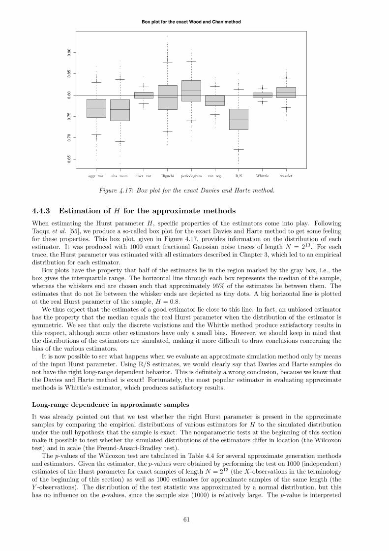
0.65
0.70
0.75
0.80
0.85
0.90
Box plot for the exact Wood and Chan method
PSfrag
replacem
ents
log2 (N
)nk
aggr. var. abs. mom. discr. var. Higuchi periodogram var. reg. R/S Whittle wavelet
Figure 4.17: Box plot for the exact Davies and Harte method.
4.4.3 Estimation of H for the approximate methods
When estimating the Hurst parameter H, specific properties of the estimators come into play. FollowingTaqqu et al. [55], we produce a so-called box plot for the exact Davies and Harte method to get some feelingfor these properties. This box plot, given in Figure 4.17, provides information on the distribution of eachestimator. It was produced with 1000 exact fractional Gaussian noise traces of length N = 213. For eachtrace, the Hurst parameter was estimated with all estimators described in Chapter 3, which led to an empiricaldistribution for each estimator.
Box plots have the property that half of the estimates lie in the region marked by the gray box, i.e., thebox gives the interquartile range. The horizontal line through each box represents the median of the sample,whereas the whiskers end are chosen such that approximately 95% of the estimates lie between them. Theestimates that do not lie between the whisker ends are depicted as tiny dots. A big horizontal line is plottedat the real Hurst parameter of the sample, H = 0.8.
We thus expect that the estimates of a good estimator lie close to this line. In fact, an unbiased estimatorhas the property that the median equals the real Hurst parameter when the distribution of the estimator issymmetric. We see that only the discrete variations and the Whittle method produce satisfactory results inthis respect, although some other estimators have only a small bias. However, we should keep in mind thatthe distributions of the estimators are simulated, making it more difficult to draw conclusions concerning thebias of the various estimators.
It is now possible to see what happens when we evaluate an approximate simulation method only by meansof the input Hurst parameter. Using R/S estimates, we would clearly say that Davies and Harte samples donot have the right long-range dependent behavior. This is definitely a wrong conclusion, because we know thatthe Davies and Harte method is exact! Fortunately, the most popular estimator in evaluating approximatemethods is Whittle’s estimator, which produces satisfactory results.
Long-range dependence in approximate samples
It was already pointed out that we test whether the right Hurst parameter is present in the approximatesamples by comparing the empirical distributions of various estimators for H to the simulated distributionunder the null hypothesis that the sample is exact. The nonparametric tests at the beginning of this sectionmake it possible to test whether the simulated distributions of the estimators differ in location (the Wilcoxontest) and in scale (the Freund-Ansari-Bradley test).
The p-values of the Wilcoxon test are tabulated in Table 4.4 for several approximate generation methodsand estimators. Given the estimator, the p-values were obtained by performing the test on 1000 (independent)estimates of the Hurst parameter for exact samples of length N = 213 (the X-observations in the terminologyof the beginning of this section) as well as 1000 estimates for approximate samples of the same length (theY -observations). The distribution of the test statistic was approximated by a normal distribution, but thishas no influence on the p-values, since the sample size (1000) is relatively large. The p-value is interpreted
61
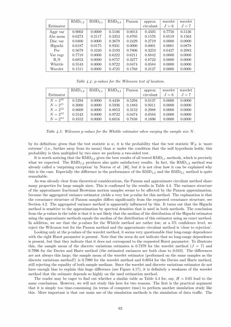
RMD1,2 RMD2,1 RMD3,3 Paxson approx. wavelet waveletEstimator circulant J = 6 J = 7
Aggr var 0.9002 0.0009 0.5106 0.0013 0.4505 0.7750 0.5136Abs mom 0.6273 0.2117 0.2352 0.8705 0.1576 0.0519 0.1563Disc var 0.0400 0.0000 0.2679 0.2429 0.2719 0.0000 0.0000Higuchi 0.6187 0.0175 0.9331 0.0000 0.0001 0.0001 0.0878
Per 0.5679 0.4240 0.2193 0.7806 0.3253 0.0427 0.2983Var regr 0.7718 0.0000 0.6222 0.6211 0.8842 0.0000 0.0000
R/S 0.6853 0.0000 0.8757 0.3277 0.8722 0.0000 0.0000Whittle 0.5543 0.0000 0.9722 0.0474 0.0584 0.0000 0.0000Wavelet 0.1511 0.0000 0.4725 0.1768 0.2127 0.0000 0.0000
Table 4.4: p-values for the Wilcoxon test of location.
RMD1,2 RMD2,1 RMD3,3 Paxson approx. wavelet waveletEstimator circulant J = 6 J = 7
N = 210 0.5294 0.0000 0.4438 0.5294 0.0137 0.0000 0.0000N = 211 0.3000 0.0000 0.5936 0.1883 0.9311 0.0000 0.0000N = 212 0.8609 0.0000 0.8853 0.3152 0.2988 0.0000 0.0000N = 213 0.5543 0.0000 0.9722 0.0474 0.0584 0.0000 0.0000N = 214 0.4552 0.0000 0.6016 0.7838 0.1696 0.0000 0.0000
Table 4.5: Wilcoxon p-values for the Whittle estimator when varying the sample size N .
by its definition; given that the test statistic is w, it is the probability that the test statistic WN is ‘moreextreme’ (i.e., further away from its mean) than w under the condition that the null hypothesis holds; thisprobability is then multiplied by two since we perform a two-sided test.
It is worth noticing that the RMD3,3 gives the best results of all tested RMDl,r methods, which is preciselywhat we expected. The RMD1,2 produces also quite satisfactory results. In fact, the RMD1,2 method wasalready called a ‘surprising exception’ by Norros et al. [46], but it is not clear how it can be explained whythis is the case. Especially the difference in the performance of the RMD1,2 and the RMD2,1 method is quiteremarkable.
As was already clear from theoretical considerations, the Paxson and approximate circulant method sharemany properties for large sample sizes. This is confirmed by the results in Table 4.4. The variance structureof the approximate fractional Brownian motion samples seems to be affected by the Paxson approximation,because the aggregated variance estimator yields a very low p-value for this method. The explanation is thatthe covariance structure of Paxson samples differs significantly from the requested covariance structure, seeSection 4.2. The aggregated variance method is apparently influenced by this. It turns out that the Higuchimethod is sensitive to the approximation by spectral densities that is used in both methods. The conclusionfrom the p-values in the table is that it is not likely that the median of the distribution of the Higuchi estimatorusing the approximate methods equals the median of the distribution of this estimator using an exact method.In addition, we see that the p-values for the Whittle method are rather low; at a 5% confidence level, wereject the Wilcoxon test for the Paxson method and the approximate circulant method is ‘close to rejection’.
Looking only at the p-values of the wavelet method, it seems very questionable that long-range dependencewith the right Hurst parameter is present. Note that the zeros do not indicate that no long-range dependenceis present, but that they indicate that it does not correspond to the requested Hurst parameter. To illustratethis, the sample mean of the discrete variations estimates is 0.7379 for the wavelet method (J = 7) and0.7996 for the Davies and Harte method (the estimated variances are both close to 0.010). The differencesare not always this large; the sample mean of the wavelet estimator (performed on the same samples as thediscrete variations method!) is 0.7980 for the wavelet method and 0.8054 for the Davies and Harte method,still rejecting the equality of both sample medians. Since the wavelet and discrete variations estimator do nothave enough bias to explain this huge difference (see Figure 4.17), it is definitely a weakness of the waveletmethod that the estimate depends so highly on the used estimation method.
The reader may be eager to find out whether a similar table as Table 4.4 for, say, H = 0.65 lead to thesame conclusions. However, we will not study this here for two reasons. The first is the practical argumentthat it is simply too time-consuming (in terms of computer time) to perform another simulation study likethis. More important is that our main use of the simulation methods is the simulation of data traffic. The
62
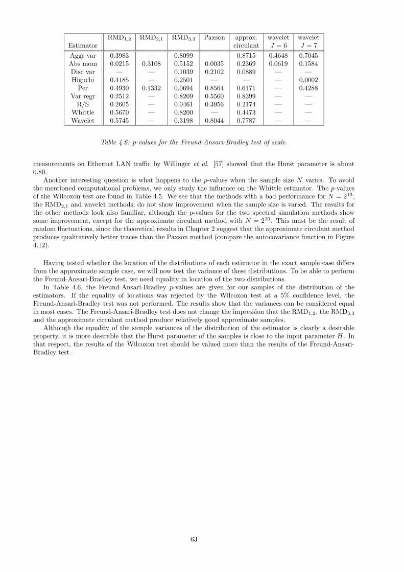
RMD1,2 RMD2,1 RMD3,3 Paxson approx. wavelet waveletEstimator circulant J = 6 J = 7
Aggr var 0.3983 — 0.8099 — 0.8715 0.4648 0.7045Abs mom 0.0215 0.3108 0.5152 0.0035 0.2369 0.0619 0.1584Disc var — — 0.1039 0.2102 0.0889 — —Higuchi 0.4185 — 0.2501 — — — 0.0002
Per 0.4930 0.1332 0.0694 0.8564 0.6171 — 0.4288Var regr 0.2512 — 0.8209 0.5560 0.8399 — —
R/S 0.2605 — 0.0461 0.3956 0.2174 — —Whittle 0.5670 — 0.8200 — 0.4473 — —Wavelet 0.5745 — 0.3198 0.8044 0.7787 — —
Table 4.6: p-values for the Freund-Ansari-Bradley test of scale.
measurements on Ethernet LAN traffic by Willinger et al. [57] showed that the Hurst parameter is about0.80.
Another interesting question is what happens to the p-values when the sample size N varies. To avoidthe mentioned computational problems, we only study the influence on the Whittle estimator. The p-valuesof the Wilcoxon test are found in Table 4.5. We see that the methods with a bad performance for N = 213,the RMD2,1 and wavelet methods, do not show improvement when the sample size is varied. The results forthe other methods look also familiar, although the p-values for the two spectral simulation methods showsome improvement, except for the approximate circulant method with N = 210. This must be the result ofrandom fluctuations, since the theoretical results in Chapter 2 suggest that the approximate circulant methodproduces qualitatively better traces than the Paxson method (compare the autocovariance function in Figure4.12).
Having tested whether the location of the distributions of each estimator in the exact sample case differsfrom the approximate sample case, we will now test the variance of these distributions. To be able to performthe Freund-Ansari-Bradley test, we need equality in location of the two distributions.
In Table 4.6, the Freund-Ansari-Bradley p-values are given for our samples of the distribution of theestimators. If the equality of locations was rejected by the Wilcoxon test at a 5% confidence level, theFreund-Ansari-Bradley test was not performed. The results show that the variances can be considered equalin most cases. The Freund-Ansari-Bradley test does not change the impression that the RMD1,2, the RMD3,3
and the approximate circulant method produce relatively good approximate samples.Although the equality of the sample variances of the distribution of the estimator is clearly a desirable
property, it is more desirable that the Hurst parameter of the samples is close to the input parameter H. Inthat respect, the results of the Wilcoxon test should be valued more than the results of the Freund-Ansari-Bradley test.
63
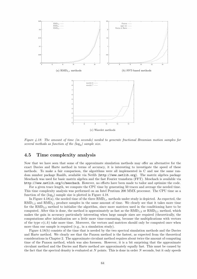
0
0.05
0.1
0.15
0.2
0.25
4 6 8 10 12 14
PSfrag
replacem
ents
log2 (N
)nk
RMD1,2
RMD2,1
RMD3,3
(a) RMDl,r methods
0
0.5
1
1.5
2
2.5
4 6 8 10 12 14
PSfrag
replacem
ents
log2 (N
)nkR
MD
1,2R
MD
2,1R
MD
3,3
Paxsonappr circ
Davies & Harte
(b) FFT-based methods
0
1
2
3
4
5
6
7
8
9
4 6 8 10 12 14
PSfrag
replacem
ents
log2 (N
)nkR
MD
1,2R
MD
2,1R
MD
3,3Paxson
appr
circD
avies&
Harte
wavelet 6wavelet 7
(c) Wavelet methods
Figure 4.18: The amount of time (in seconds) needed to generate fractional Brownian motion samples forseveral methods as function of the (log2) sample size.
4.5 Time complexity analysis
Now that we have seen that some of the approximate simulation methods may offer an alternative for theexact Davies and Harte method in terms of accuracy, it is interesting to investigate the speed of thesemethods. To make a fair comparison, the algorithms were all implemented in C and use the same ran-dom number package Ranlib, available via Netlib (http://www.netlib.org). The matrix algebra packageMeschach was used for basic matrix algebra and the fast Fourier transform (FFT). Meschach is available viahttp://www.netlib.org/c/meschach. However, no efforts have been made to tailor and optimize the code.
For a given trace length, we compute the CPU time by generating 50 traces and average the needed time.This time complexity analysis was performed on an Intel Pentium 200 MMX processor. The CPU time as afunction of the (log2) sample size is plotted in Figure 4.18.
In Figure 4.18(a), the needed time of the three RMDl,r methods under study is depicted. As expected, theRMD1,2 and RMD2,1 produce samples in the same amount of time. We clearly see that it takes more timefor the RMD3,3 method to initialize the algorithm, since more matrices used in the conditioning have to becomputed. After this is done, the method is approximately as fast as the RMD1,2 or RMD2,1 method, whichmakes the gain in accuracy particularly interesting when large sample sizes are required (theoretically, thecomputations after initialization are a little more time-consuming, because the multiplications with vectorsof the type e(i, k) take more time. Moreover, the vectors and matrices should only be computed once whenmore than one sample is required (e.g., in a simulation study).
Figure 4.18(b) consists of the time that is needed by the two spectral simulation methods and the Daviesand Harte method. We clearly see that the Paxson method is the fastest, as expected from the theoreticalconsiderations in Chapter 2. The approximate circulant method requires about twice the amount of computingtime of the Paxson method, which was also foreseen. However, it is a bit surprising that the approximatecirculant method and the Davies and Harte method are approximately equally fast. This must be caused bythe fact that the spectral density is evaluated at N points. This is done in order N seconds, but it only speeds
64

-8
-7
-6
-5
-4
-3
-2
-1
4 6 8 10 12 14
PSfrag
replacem
ents
log2 (N
)nk
RMD1,2
RMD2,1
RMD3,3
(a) RMDl,r methods
-10
-8
-6
-4
-2
0
2
4 6 8 10 12 14 16 18 20
PSfrag
replacem
ents
log2 (N
)nkR
MD
1,2R
MD
2,1R
MD
3,3
Paxsonappr circ
Davies & Harte
(b) FFT-based methods
Figure 4.19: A function of the amount of time such that a straight line should appear for large N .
up the algorithm when N is large enough (since an FFT operation of order N log(N) seconds is saved). Wealso see this in the plot, because the curve for the Davies and Harte method is steeper for larger sample sizes.
At first sight, the plot of the computing time for the wavelet method in Figure 4.18(c) looks a bit strange,but it is possible to explain its most important features. For small sample sizes, the graph looks almost flat andincreases only a bit. In fact, the length of the fractional ARIMA trace that is used as input in the algorithmincreases only by a small amount when the number of required sample points is doubled. This has to do withthe fact that this input trace has to be convolved a couple of times. When convolving sequences, one hasto deal with border effects, i.e., the effect that the resulting sequence is spoiled by the lack of data at the‘border’ of the sequences. To avoid these border effects from influencing the sample, the length of the inputfractional ARIMA trace is increased by a fixed amount; we can think of this as a safety margin. This safetymargin is relatively large for small sample sizes, whereas its influence on the speed vanishes asymptotically.
Although this may sound reasonable, it is not plausible that this causes such a flat behavior in thecomputing time. Something else must play a role, which has to do with the convolution operation as well.This convolution was implemented with the FFT algorithm, but the lengths of the input sequences are notnecessarily a power of two. When this is not the case, zeros have to be padded to make the length a power oftwo. It is very well possible that an increase in the requested sample size has then no influence on the lengthof the extended (i.e., padded) sequences. This explains that the computation time doubles instantaneouslyfor certain sample sizes. It can not be observed in the plot that this happens instantaneously, since the graphwas interpolated; the time complexity was only computed for N = 24, 25, . . . , 215.
Theoretically, the RMDl,r method is an order N algorithm. However, this can not be checked from the plotin Figure 4.18(a). It can also not be observed for the FFT-based methods and the wavelet method that theircomplexity is N log(N). Still, we can graphically check these assertions for the RMDl,r and the FFT-basedmethods. For this, plots that should yield straight lines (at least for large N) are most suitable, see Figure4.19.
Instead of the time, the log time is plotted against the log sample size for the RMDl,r method in Figure4.19(a), yielding indeed a straight line for ‘large’ log(N). To achieve the same for the FFT-based methods,log log(N) is substracted from the log time. A plot for the wavelet method is not included in Figure 4.19,because only three ‘efficient’ data points are available, since much computing time is spoiled by the paddedzeros in the FFT algorithm. These efficient data points are the points at which the graph in Figure 4.18(c)‘jumps’.
A clear straight line can be observed in Figure 4.19(a) for large N , which is also true for the Paxson andapproximate circulant method in Figure 4.19(b). Note that the sample size ranges from N = 24 to N = 220
to make it possible to see a similar behavior for the Davies and Harte method, although it may require evenlarger sample sizes to make it more clear. Recall from Chapter 2 that for very large N , the approximatecirculant method should be about twice as fast as the Davies and Harte method. Since the Paxson methodis twice as fast as the approximate circulant method, the approximate circulant line should lie exactly in themiddle between the Davies and Harte line and the Paxson line. This is not the case (yet) for N = 220.
Now that we have understood the shape of the time complexity graphs, we are able to draw conclusionson the accuracy-speed trade-off.
65


CHAPTER 5
Conclusions
In this report, several methods to simulate fractional Brownian motion were described and discussed. Thethree (theoretically) most promising ‘families’ of methods were evaluated:
• The RMDl,r method proposed by Norros et al. [46];
• The Paxson method proposed by Paxson [47] and a generalization of the Paxson method, the approxi-mate circulant method;
• A wavelet-based simulation method by Abry and Sellan [2].
A fair comparison between different methods is a difficult task. Almost any method can be favoured abovethe others by changing the comparison criterion. In this report, the comparison was made by an error analysisand by checking theoretically or statistically a number of properties that fully characterize fractional Brownianmotion: besides that the sample should be centered and Gaussian, its increments should be stationary. Theproperty that the variance at time t should be t2H was checked by estimating the Hurst parameter withvarious estimators.
We arrive at the following conclusions:
• So-called spectral simulation provides the theoretical foundation for the Paxson method, which clarifiesmany empirical observations and leads to an important improvement of the method. Moreover, a naturalextension of the Paxson method, the approximate circulant method, has a direct connection with theexact Davies and Harte method. The obtained insights show that the accuracy of both methods increasesas the sample size grows, and that the methods are even asymptotically exact in the sense that thefinite-dimensional distributions of the approximate sample converge in probability to the correspondingdistributions of the exact sample.
• These insights make it also possible to perform an error analysis for the approximate circulant method,in which the theoretical results are confirmed. The same errors can be analyzed for the RMD1,2 method,which shows better performance.
• The covariance structure of approximate Paxson samples, approximate circulant samples and RMDl,r
samples can numerically be calculated. Since all approximate methods under study produce zero-meanGaussian samples, these covariances fully characterize the approximate method. While the errors in thecovariances are quite big for the Paxson method (although they vanish asymptotically), the autocovari-ance function of the approximate circulant method is visually almost indistinguishable from the exactautocovariance function. Still, this autocovariance function does not show the desired hyperbolical tailbehavior.
• Since the RMDl,r produces in general non-stationary samples, it takes more effort to study the tailbehavior of the covariances. We showed how the covariances of an RMDl,r sample can numerically becomputed for general l ≥ 0 and r ≥ 1. An analysis of these covariances of the RMD1,2 and the RMD3,3
method showed that these methods also do not have the desired decay in the covariances. This can beimproved by removing some begin and end points in the approximate RMDl,r sample.
• The overall impression from the accuracy analysis is that only the RMD1,2, the RMD3,3, and theapproximate circulant method are reasonable alternatives for the exact Davies and Harte method.
67
• The wavelet method studied in this report is disappointing, in terms of both speed and accuracy,although theoretically the time complexity is approximately N log(N).
• The RMDl,r method is the only studied method of which the time complexity grows linearly in thetrace length. Since the extra time needed by the RMD3,3 compared to the RMD1,2 method is almostnegligible, the RMD3,3 method is the most interesting.
• The Paxson method is faster than the exact Davies and Harte method, while the approximate circulantmethod is only faster for relatively large sample sizes. As mentioned earlier, their accuracy also improvesas the trace length grows. Since they are based on the FFT, these methods have time complexityN log(N).
From these observations, a final choice is readily made: the RMD3,3 method. Moreover, it is possibleto generate RMD3,3 samples on-the-fly, which is an advantage that is not shared by the Davies and Hartemethod (nor by the two spectral methods). In both methods it is possible to ‘recycle’ some computationswhen more samples of the same size are needed, but the RMD3,3 method stays an order N method, and theDavies and Harte an order N log(N) method.
However, in a simulation study, for instance, it may be far more desirable to know that the samples areexact. Therefore, the Davies and Harte method should be used in principle. When long traces or manyruns are needed in a simulation study, it may computationally be impossible to generate exact samples. TheRMD3,3 method is then a good alternative.
Before celebrating the RMDl,r method too much, we have also seen in a study of the relative error in anetwork model that the approximate circulant method performs in this model better than the RMD1,2 methodfor reasonable sample sizes. This indicates that our conclusions are not as robust as they may seem. If theapproximate method is not first evaluated in the framework in which it is used, it is quite risky to just use anapproximate method. This is particularly the case when rare events are simulated, e.g., loss probabilities inqueues. The use of approximate methods should thus be avoided, especially since a quite fast exact algorithmexists.
68
Bibliography
[1] P. Abry, P. Goncalves, and P. Flandrin, Wavelets, spectrum analysis and 1/f processes, inWavelets and statistics, A. Antoniadis and G. Oppenheim, eds., vol. 103 of Lecture Notes in Statis-tics, Springer-Verlag, New York, 1995, pp. 15–30.
[2] P. Abry and F. Sellan, The wavelet-based synthesis for fractional Brownian motion proposed by F.Sellan and Y. Meyer: remarks and fast implemention, Applied and computational harmonic analysis, 3(1996), pp. 377–383.
[3] P. Abry and D. Veitch, Wavelet analysis of long range dependent traffic, IEEE Transactions onInformation Theory, 44 (1998), pp. 2–15.
[4] S. Asmussen, Stochastic simulation with a view towards stochastic processes. Notes of a ConcentratedAdvance Course at MaPhySto, Aarhus, Denmark, February 1999.
[5] A. Ayache and M. S. Taqqu, Approximating fractional Brownian motion by a random wavelet series:the rate optimality problem. To appear in J. Fourier Anal. Appl., 2003.
[6] J.B. Bassingthwaighte and G.M. Raymond, Evaluating rescaled range analysis for time series,Annals of Biomedical Engineering, 22 (1994), pp. 432–444.
[7] , Evaluation of the dispersional analysis method for fractal time series, Annals of Biomedical Engi-neering, 23 (1995), pp. 491–505.
[8] J. Beran, A goodness-of-fit test for time series with long range dependence, J. R. Statist. Soc. B, 54(1992), pp. 749–760.
[9] , Statistics for long-memory processes, no. 61 in Monographs on statistics and applied probability,Chapman and Hall, 1994.
[10] J. Beran, R. Sherman, M.S. Taqqu, and W. Willinger, Long-range dependence in variable-bit-ratevideo traffic, IEEE Trans. on Communications, 43 (1995), pp. 1566–1579.
[11] P.J. Brockwell and R.A. Davis, Time series: Theory and methods, Springer-Verlag, New York,1987.
[12] M.J. Cannon, D.B. Percival, D.C. Caccia, G.M. Raymond, and J.B. Bassingthwaighte,Evaluating scaled windowed variance methods for estimating the Hurst coefficient of time series, PhysicaA, 241 (1997), pp. 606–626.
[13] K. L. Chung, A Course in Probability Theory, Academic Press, San Diego, third ed., 2001.
[14] J.F. Coeurjolly, Inference statistique pour les mouvements browniens fractionnaires et multifraction-naires, PhD thesis, Universite Joseph Fourier, Dec. 2000.
[15] , Simulation and identification of the fractional Brownian motion: a bibliographical and comparativestudy, Journal of Stat. Software, 5 (2000). Available from http://www.jstatsoft.org.
[16] D.R. Cox, Long-range dependence: a review, in Statistics: an appraisal, H.A. David and H.T. David,eds., Iowa State University Press, 1984, pp. 55–74.
[17] M. S. Crouse and R. G. Baraniuk, Fast, exact synthesis of Gaussian and nonGaussian long-rangedependent processes. Submitted to IEEE Transactions on Information Theory, 1999.
[18] I. Daubechies, Ten lectures on wavelets, CBMS-NSF Regional Conference Series, SIAM, 1992.
69
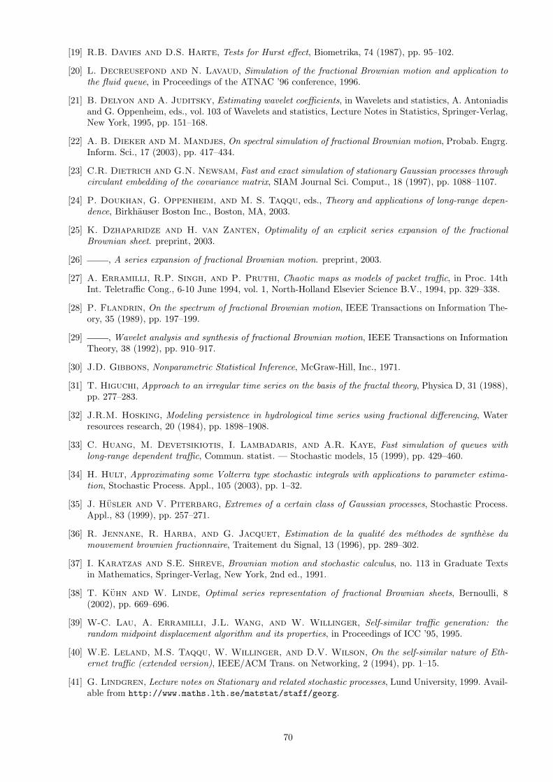
[19] R.B. Davies and D.S. Harte, Tests for Hurst effect, Biometrika, 74 (1987), pp. 95–102.
[20] L. Decreusefond and N. Lavaud, Simulation of the fractional Brownian motion and application tothe fluid queue, in Proceedings of the ATNAC ’96 conference, 1996.
[21] B. Delyon and A. Juditsky, Estimating wavelet coefficients, in Wavelets and statistics, A. Antoniadisand G. Oppenheim, eds., vol. 103 of Wavelets and statistics, Lecture Notes in Statistics, Springer-Verlag,New York, 1995, pp. 151–168.
[22] A. B. Dieker and M. Mandjes, On spectral simulation of fractional Brownian motion, Probab. Engrg.Inform. Sci., 17 (2003), pp. 417–434.
[23] C.R. Dietrich and G.N. Newsam, Fast and exact simulation of stationary Gaussian processes throughcirculant embedding of the covariance matrix, SIAM Journal Sci. Comput., 18 (1997), pp. 1088–1107.
[24] P. Doukhan, G. Oppenheim, and M. S. Taqqu, eds., Theory and applications of long-range depen-dence, Birkhauser Boston Inc., Boston, MA, 2003.
[25] K. Dzhaparidze and H. van Zanten, Optimality of an explicit series expansion of the fractionalBrownian sheet. preprint, 2003.
[26] , A series expansion of fractional Brownian motion. preprint, 2003.
[27] A. Erramilli, R.P. Singh, and P. Pruthi, Chaotic maps as models of packet traffic, in Proc. 14thInt. Teletraffic Cong., 6-10 June 1994, vol. 1, North-Holland Elsevier Science B.V., 1994, pp. 329–338.
[28] P. Flandrin, On the spectrum of fractional Brownian motion, IEEE Transactions on Information The-ory, 35 (1989), pp. 197–199.
[29] , Wavelet analysis and synthesis of fractional Brownian motion, IEEE Transactions on InformationTheory, 38 (1992), pp. 910–917.
[30] J.D. Gibbons, Nonparametric Statistical Inference, McGraw-Hill, Inc., 1971.
[31] T. Higuchi, Approach to an irregular time series on the basis of the fractal theory, Physica D, 31 (1988),pp. 277–283.
[32] J.R.M. Hosking, Modeling persistence in hydrological time series using fractional differencing, Waterresources research, 20 (1984), pp. 1898–1908.
[33] C. Huang, M. Devetsikiotis, I. Lambadaris, and A.R. Kaye, Fast simulation of queues withlong-range dependent traffic, Commun. statist. — Stochastic models, 15 (1999), pp. 429–460.
[34] H. Hult, Approximating some Volterra type stochastic integrals with applications to parameter estima-tion, Stochastic Process. Appl., 105 (2003), pp. 1–32.
[35] J. Husler and V. Piterbarg, Extremes of a certain class of Gaussian processes, Stochastic Process.Appl., 83 (1999), pp. 257–271.
[36] R. Jennane, R. Harba, and G. Jacquet, Estimation de la qualite des methodes de synthese dumouvement brownien fractionnaire, Traitement du Signal, 13 (1996), pp. 289–302.
[37] I. Karatzas and S.E. Shreve, Brownian motion and stochastic calculus, no. 113 in Graduate Textsin Mathematics, Springer-Verlag, New York, 2nd ed., 1991.
[38] T. Kuhn and W. Linde, Optimal series representation of fractional Brownian sheets, Bernoulli, 8(2002), pp. 669–696.
[39] W-C. Lau, A. Erramilli, J.L. Wang, and W. Willinger, Self-similar traffic generation: therandom midpoint displacement algorithm and its properties, in Proceedings of ICC ’95, 1995.
[40] W.E. Leland, M.S. Taqqu, W. Willinger, and D.V. Wilson, On the self-similar nature of Eth-ernet traffic (extended version), IEEE/ACM Trans. on Networking, 2 (1994), pp. 1–15.
[41] G. Lindgren, Lecture notes on Stationary and related stochastic processes, Lund University, 1999. Avail-able from http://www.maths.lth.se/matstat/staff/georg.
70
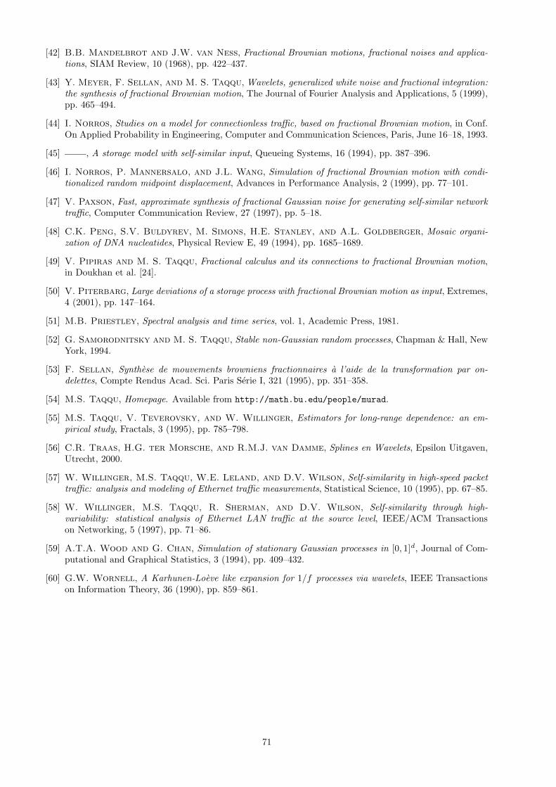
[42] B.B. Mandelbrot and J.W. van Ness, Fractional Brownian motions, fractional noises and applica-tions, SIAM Review, 10 (1968), pp. 422–437.
[43] Y. Meyer, F. Sellan, and M. S. Taqqu, Wavelets, generalized white noise and fractional integration:the synthesis of fractional Brownian motion, The Journal of Fourier Analysis and Applications, 5 (1999),pp. 465–494.
[44] I. Norros, Studies on a model for connectionless traffic, based on fractional Brownian motion, in Conf.On Applied Probability in Engineering, Computer and Communication Sciences, Paris, June 16–18, 1993.
[45] , A storage model with self-similar input, Queueing Systems, 16 (1994), pp. 387–396.
[46] I. Norros, P. Mannersalo, and J.L. Wang, Simulation of fractional Brownian motion with condi-tionalized random midpoint displacement, Advances in Performance Analysis, 2 (1999), pp. 77–101.
[47] V. Paxson, Fast, approximate synthesis of fractional Gaussian noise for generating self-similar networktraffic, Computer Communication Review, 27 (1997), pp. 5–18.
[48] C.K. Peng, S.V. Buldyrev, M. Simons, H.E. Stanley, and A.L. Goldberger, Mosaic organi-zation of DNA nucleatides, Physical Review E, 49 (1994), pp. 1685–1689.
[49] V. Pipiras and M. S. Taqqu, Fractional calculus and its connections to fractional Brownian motion,in Doukhan et al. [24].
[50] V. Piterbarg, Large deviations of a storage process with fractional Brownian motion as input, Extremes,4 (2001), pp. 147–164.
[51] M.B. Priestley, Spectral analysis and time series, vol. 1, Academic Press, 1981.
[52] G. Samorodnitsky and M. S. Taqqu, Stable non-Gaussian random processes, Chapman & Hall, NewYork, 1994.
[53] F. Sellan, Synthese de mouvements browniens fractionnaires a l’aide de la transformation par on-delettes, Compte Rendus Acad. Sci. Paris Serie I, 321 (1995), pp. 351–358.
[54] M.S. Taqqu, Homepage. Available from http://math.bu.edu/people/murad.
[55] M.S. Taqqu, V. Teverovsky, and W. Willinger, Estimators for long-range dependence: an em-pirical study, Fractals, 3 (1995), pp. 785–798.
[56] C.R. Traas, H.G. ter Morsche, and R.M.J. van Damme, Splines en Wavelets, Epsilon Uitgaven,Utrecht, 2000.
[57] W. Willinger, M.S. Taqqu, W.E. Leland, and D.V. Wilson, Self-similarity in high-speed packettraffic: analysis and modeling of Ethernet traffic measurements, Statistical Science, 10 (1995), pp. 67–85.
[58] W. Willinger, M.S. Taqqu, R. Sherman, and D.V. Wilson, Self-similarity through high-variability: statistical analysis of Ethernet LAN traffic at the source level, IEEE/ACM Transactionson Networking, 5 (1997), pp. 71–86.
[59] A.T.A. Wood and G. Chan, Simulation of stationary Gaussian processes in [0, 1]d, Journal of Com-putational and Graphical Statistics, 3 (1994), pp. 409–432.
[60] G.W. Wornell, A Karhunen-Loeve like expansion for 1/f processes via wavelets, IEEE Transactionson Information Theory, 36 (1990), pp. 859–861.
71