Simulation of Droplet Dynamics and Mixing in … of Droplet Dynamics and Mixing in ... is an...

Sensors & Transducers Journal, Vol.0, Issue 0, Month 2009, pp.

SSSeeennnsssooorrrsss &&& TTTrrraaannnsssddduuuccceeerrrsss

ISSN 1726-5479© 2009 by IFSA

http://www.sensorsportal.com

Simulation of Droplet Dynamics and Mixing in Microfluidic Devices using a VOF-Based Method

Anurag CHANDORKAR, Shayan PALIT

Flow Science Inc., 683 Harkle Rd, Ste A, Santa Fe, NM 87505, USA Phone: 505-982-0088, Fax: 505-982-5551, Email: [email protected]

Received: /Accepted: /Published: Abstract: This paper demonstrates that the Volume of Fluid (TruVOF®) method in FLOW-3D® (a general purpose CFD software) is an effective tool for studying droplet dynamics and mixing in microfluidic devices. The first example studied is a T-junction where flow patterns for both droplet generation and passive mixing are analyzed. The second example studied is a co-flowing device where the formation and breakup of bubbles is simulated. The effect of viscosity on bubble formation is also analyzed. For a T-junction the bubble size is corroborated with experimental data. Both the bubble size and frequency are studied and corroborated with experimental data for a co-flowing device. The third example studied is the electrowetting phenomenon observed in a small water droplet resting on a dielectric material. The steady-state contact angle is plotted against the voltage applied. The results are compared with both the Young-Lippmann curve and experimental results. Keywords: droplet-based microfluidic devices, co-flowing devices, T-junction, electrowetting, volume of fluid method 1. Introduction There has been considerable interest in the study of droplet formation and passive mixing in microfluidics devices recently. These devices have several applications, for example, on-chip separation, chemical reactions and biochemical synthesis [1]. A related phenomenon that has also garnered much interest recently is electrowetting. This phenomenon can be used to manipulate small liquid droplets on solid surfaces. Applications include Lab on a Chip devices, electronic displays and adjustable lenses [2]. In this paper we will show a Volume of Fluid (VOF) based algorithm to be an effective simulation tool for studying and characterizing the dynamics of droplets in these micro-scale devices.


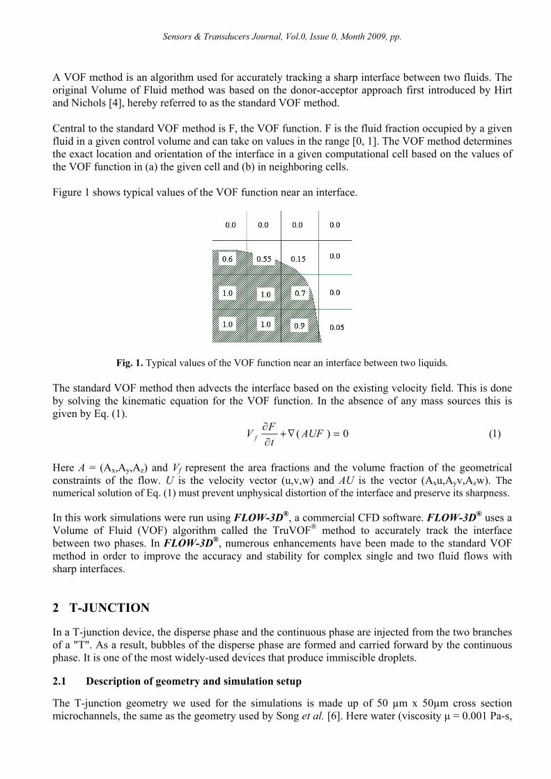
A VOF method is an algorithm used for accurately tracking a sharp interface between two fluids. The original Volume of Fluid method was based on the donor-acceptor approach first introduced by Hirt and Nichols [4], hereby referred to as the standard VOF method. Central to the standard VOF method is F, the VOF function. F is the fluid fraction occupied by a given fluid in a given control volume and can take on values in the range [0, 1]. The VOF method determines the exact location and orientation of the interface in a given computational cell based on the values of the VOF function in (a) the given cell and (b) in neighboring cells. Figure 1 shows typical values of the VOF function near an interface.

Fig. 1. Typical values of the VOF function near an interface between two liquids.

The standard VOF method then advects the interface based on the existing velocity field. This is done by solving the kinematic equation for the VOF function. In the absence of any mass sources this is given by Eq. (1).

)1(0)(∇∂∂ =+ AUF

tFV f

Here A = (Ax,Ay,Az) and Vf represent the area fractions and the volume fraction of the geometrical constraints of the flow. U is the velocity vector (u,v,w) and AU is the vector (Axu,Ayv,Azw). The numerical solution of Eq. (1) must prevent unphysical distortion of the interface and preserve its sharpness. In this work simulations were run using FLOW-3D®, a commercial CFD software. FLOW-3D® uses a Volume of Fluid (VOF) algorithm called the TruVOF® method to accurately track the interface between two phases. In FLOW-3D®, numerous enhancements have been made to the standard VOF method in order to improve the accuracy and stability for complex single and two fluid flows with sharp interfaces. 2 T-JUNCTION

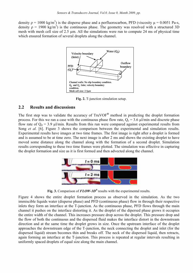
In a T-junction device, the disperse phase and the continuous phase are injected from the two branches of a "T". As a result, bubbles of the disperse phase are formed and carried forward by the continuous phase. It is one of the most widely-used devices that produce immiscible droplets.

2.1 Description of geometry and simulation setup

The T-junction geometry we used for the simulations is made up of 50 µm x 50µm cross section microchannels, the same as the geometry used by Song et al. [6]. Here water (viscosity μ = 0.001 Pa-s,


density ρ = 1000 kg/m3) is the disperse phase and a perfluorocarbon, PFD (viscosity μ = 0.0051 Pa-s, density ρ = 1900 kg/m3) is the continuous phase. The geometry was resolved with a structured 3D mesh with mesh cell size of 2.5 µm. All the simulations were run to compute 24 ms of physical time which ensured formation of several droplets along the channel.

PFD (Qc)

Water (Qd)Velocity boundary (Inlet)

Channel walls: No slip boundary condition.Qd and Qc: Inlet, velocity boundary condition.Mesh cell size: 2.5µm

Outflow boundaryPFD

(Qc)

Water (Qd)Velocity boundary (Inlet)

Channel walls: No slip boundary condition.Qd and Qc: Inlet, velocity boundary condition.Mesh cell size: 2.5µm

Outflow boundary

Fig. 2. T-junction simulation setup.

2.2 Results and discussions

The first step was to validate the accuracy of TruVOF® method in predicting the droplet formation process. For this we ran a case with the continuous phase flow rate, Qc = 3.6 µl/min and discrete phase flow rate of Qd = 3.9 µl/min. Results from this run were compared against experimental results from Song et al. [6]. Figure 3 shows the comparison between the experimental and simulation results. Experimental results have images at two time frames. The first image is right after a droplet is formed and is assumed to be at time zero. The next image is after 2 ms and shows the existing droplet to have moved some distance along the channel along with the formation of a second droplet. Simulation results corresponding to these two time frames were plotted. The simulation was effective in capturing the droplet formation and size as it is first formed and then advected along the channel.

Fig. 3. Comparison of FLOW-3D® results with the experimental results.

Figure 4 shows the entire droplet formation process as observed in the simulation. As the two immiscible liquids water (disperse phase) and PFD (continuous phase) flow in through their respective inlets they form an interface at the T-junction. As the continuous phase, PFD flows through the main channel it pushes on the interface distorting it. As the droplet of the dipersed phase grows it occupies the entire width of the channel. This increases pressure drop across the droplet. This pressure drop and the flow of both the continuous and the dispersed fluid makes the interface distort in the downstream direction and at the same time the droplet grows in size. Once the upstream interface of the droplet approaches the downstream edge of the T-junction, the neck connecting the droplet and inlet (for the dispersed liquid) stream becomes thin and breaks off. The neck of the dispersed liquid, then retracts, again forming an interface at the T-junction. This process is repeated at regular intervals resulting in uniformly spaced droplets of equal size along the main channel.


Fig. 4. Droplet formation process in a T-junction.

The next step was to study the effect of the Qd/Qc ratio on droplet length and frequency. The Qd/Qc ratio was varied by changing the flow rate of continuous phase (Qc) from 1.8 µl/min to 7.2 µl/min while the flow rate of the disperse phase (Qd) was kept constant at (Qd = 3.9 µl/min). The simulation results in Fig. 5 show that droplet length decreases as the flow rate of the continuous phase (Qc) increases. This behavior results from the increased shearing force of the continuous phase with increased velocity. Garstecki et al. [5] conducted several experiments for a T-junction geometry and proposed a scaling law as shown in Eq. 2 to correlate the droplet length (L) and droplet width (W) with the Qd/Qc ratio. The equation has two constant parameters α and ω whose values depend on the geometry.

)(2QQα+=

wL

c

dω

Fig. 5. Increase in continuous phase flow rate (Qc) decreases bubble length. (a: Qc = 1.8 µl/min, b: Qc = 2.7 µl/min, c: Qc = 3.6 µl/min, d: Qc = 7.2 µl/min)

Qd = 3.9 µl/min for all cases.

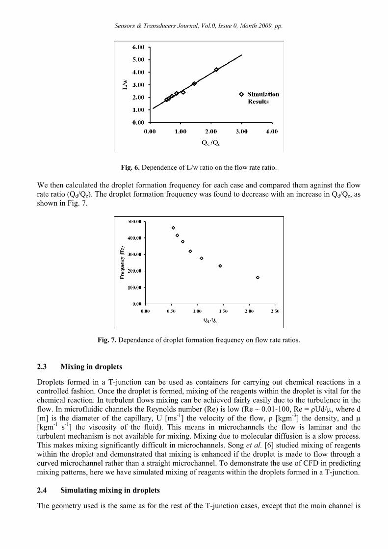
We compared the simulations results against the scaling law and found that for our T-junction geometry α is equal to 1.48 and ω is equal to 1.0. This has been shown in Fig. 6.

a b c d

e f g h

a b

c d


Fig. 6. Dependence of L/w ratio on the flow rate ratio.

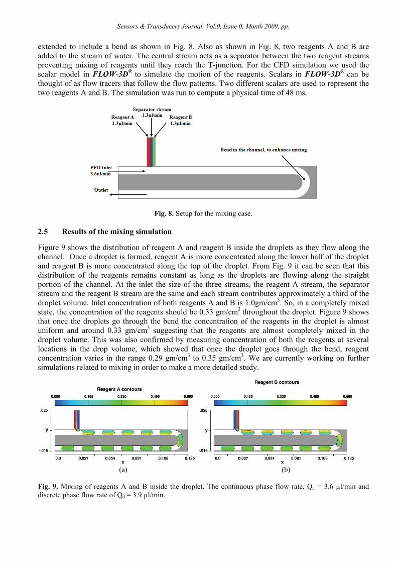
We then calculated the droplet formation frequency for each case and compared them against the flow rate ratio (Qd/Qc). The droplet formation frequency was found to decrease with an increase in Qd/Qc, as shown in Fig. 7.

Fig. 7. Dependence of droplet formation frequency on flow rate ratios.

2.3 Mixing in droplets

Droplets formed in a T-junction can be used as containers for carrying out chemical reactions in a controlled fashion. Once the droplet is formed, mixing of the reagents within the droplet is vital for the chemical reaction. In turbulent flows mixing can be achieved fairly easily due to the turbulence in the flow. In microfluidic channels the Reynolds number (Re) is low (Re ~ 0.01-100, Re = ρUd/µ, where d [m] is the diameter of the capillary, U [ms-1] the velocity of the flow, ρ [kgm-3] the density, and µ [kgm-1 s-1] the viscosity of the fluid). This means in microchannels the flow is laminar and the turbulent mechanism is not available for mixing. Mixing due to molecular diffusion is a slow process. This makes mixing significantly difficult in microchannels. Song et al. [6] studied mixing of reagents within the droplet and demonstrated that mixing is enhanced if the droplet is made to flow through a curved microchannel rather than a straight microchannel. To demonstrate the use of CFD in predicting mixing patterns, here we have simulated mixing of reagents within the droplets formed in a T-junction. 2.4 Simulating mixing in droplets

The geometry used is the same as for the rest of the T-junction cases, except that the main channel is


extended to include a bend as shown in Fig. 8. Also as shown in Fig. 8, two reagents A and B are added to the stream of water. The central stream acts as a separator between the two reagent streams preventing mixing of reagents until they reach the T-junction. For the CFD simulation we used the scalar model in FLOW-3D® to simulate the motion of the reagents. Scalars in FLOW-3D® can be thought of as flow tracers that follow the flow patterns. Two different scalars are used to represent the two reagents A and B. The simulation was run to compute a physical time of 48 ms.

Fig. 8. Setup for the mixing case.

2.5 Results of the mixing simulation

Figure 9 shows the distribution of reagent A and reagent B inside the droplets as they flow along the channel. Once a droplet is formed, reagent A is more concentrated along the lower half of the droplet and reagent B is more concentrated along the top of the droplet. From Fig. 9 it can be seen that this distribution of the reagents remains constant as long as the droplets are flowing along the straight portion of the channel. At the inlet the size of the three streams, the reagent A stream, the separator stream and the reagent B stream are the same and each stream contributes approximately a third of the droplet volume. Inlet concentration of both reagents A and B is 1.0gm/cm3. So, in a completely mixed state, the concentration of the reagents should be 0.33 gm/cm3 throughout the droplet. Figure 9 shows that once the droplets go through the bend the concentration of the reagents in the droplet is almost uniform and around 0.33 gm/cm3 suggesting that the reagents are almost completely mixed in the droplet volume. This was also confirmed by measuring concentration of both the reagents at several locations in the drop volume, which showed that once the droplet goes through the bend, reagent concentration varies in the range 0.29 gm/cm3 to 0.35 gm/cm3. We are currently working on further simulations related to mixing in order to make a more detailed study.

(a) (b) Fig. 9. Mixing of reagents A and B inside the droplet. The continuous phase flow rate, Qc = 3.6 µl/min and discrete phase flow rate of Qd = 3.9 µl/min.


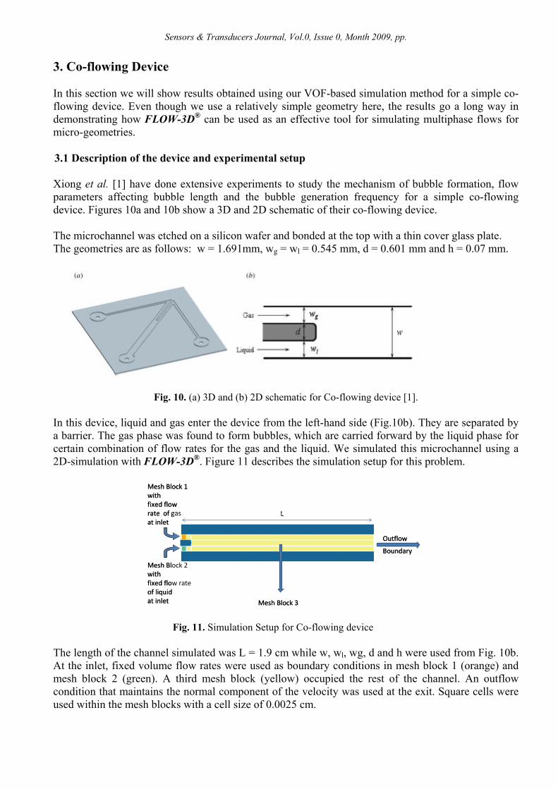
3. Co-flowing Device In this section we will show results obtained using our VOF-based simulation method for a simple co-flowing device. Even though we use a relatively simple geometry here, the results go a long way in demonstrating how FLOW-3D® can be used as an effective tool for simulating multiphase flows for micro-geometries. 3.1 Description of the device and experimental setup Xiong et al. [1] have done extensive experiments to study the mechanism of bubble formation, flow parameters affecting bubble length and the bubble generation frequency for a simple co-flowing device. Figures 10a and 10b show a 3D and 2D schematic of their co-flowing device. The microchannel was etched on a silicon wafer and bonded at the top with a thin cover glass plate. The geometries are as follows: w = 1.691mm, wg = wl = 0.545 mm, d = 0.601 mm and h = 0.07 mm.

Fig. 10. (a) 3D and (b) 2D schematic for Co-flowing device [1]. In this device, liquid and gas enter the device from the left-hand side (Fig.10b). They are separated by a barrier. The gas phase was found to form bubbles, which are carried forward by the liquid phase for certain combination of flow rates for the gas and the liquid. We simulated this microchannel using a 2D-simulation with FLOW-3D®. Figure 11 describes the simulation setup for this problem.

L

Mesh Block 1 withfixed flow rate of gasat inlet

Mesh Block 2 with fixed flow rate of liquidat inlet Mesh Block 3

Outflow

Boundary

L

Mesh Block 1 withfixed flow rate of gasat inlet

Mesh Block 2 with fixed flow rate of liquidat inlet Mesh Block 3

Outflow

Boundary

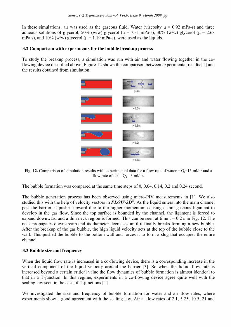
Fig. 11. Simulation Setup for Co-flowing device The length of the channel simulated was L = 1.9 cm while w, wl, wg, d and h were used from Fig. 10b. At the inlet, fixed volume flow rates were used as boundary conditions in mesh block 1 (orange) and mesh block 2 (green). A third mesh block (yellow) occupied the rest of the channel. An outflow condition that maintains the normal component of the velocity was used at the exit. Square cells were used within the mesh blocks with a cell size of 0.0025 cm.


In these simulations, air was used as the gaseous fluid. Water (viscosity μ = 0.92 mPa-s) and three aqueous solutions of glycerol, 50% (w/w) glycerol (μ = 7.31 mPa-s), 30% (w/w) glycerol (μ = 2.68 mPa s), and 10% (w/w) glycerol (μ = 1.19 mPa-s), were used as the liquids. 3.2 Comparison with experiments for the bubble breakup process To study the breakup process, a simulation was run with air and water flowing together in the co-flowing device described above. Figure 12 shows the comparison between experimental results [1] and the results obtained from simulation.

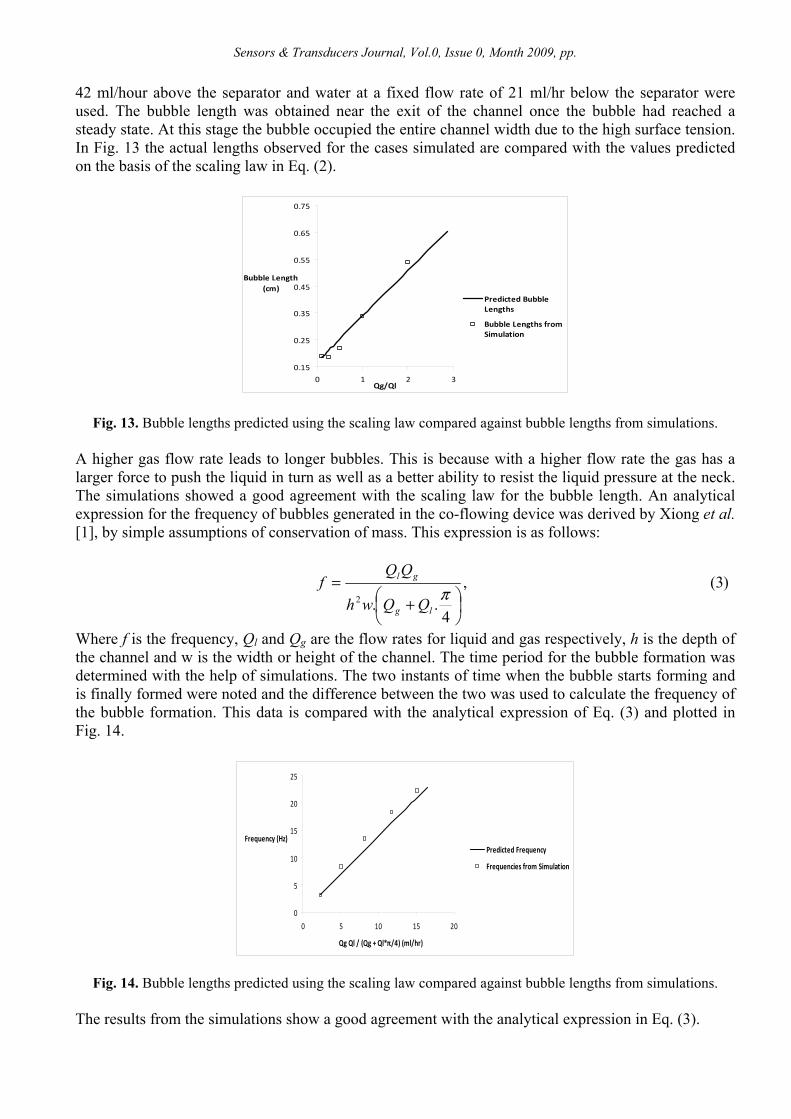
Fig. 12. Comparison of simulation results with experimental data for a flow rate of water = Ql=15 ml/hr and a flow rate of air = Qg =3 ml/hr.

The bubble formation was compared at the same time steps of 0, 0.04, 0.14, 0.2 and 0.24 second. The bubble generation process has been observed using micro-PIV measurements in [1]. We also studied this with the help of velocity vectors in FLOW-3D®. As the liquid enters into the main channel past the barrier, it pushes upward due to the higher momentum causing a thin gaseous ligament to develop in the gas flow. Since the top surface is bounded by the channel, the ligament is forced to expand downward and a thin neck region is formed. This can be seen at time t = 0.2 s in Fig. 12. The neck propagates downstream and its diameter decreases until it finally breaks forming a new bubble. After the breakup of the gas bubble, the high liquid velocity acts at the top of the bubble close to the wall. This pushed the bubble to the bottom wall and forces it to form a slug that occupies the entire channel. 3.3 Bubble size and frequency When the liquid flow rate is increased in a co-flowing device, there is a corresponding increase in the vertical component of the liquid velocity around the barrier [3]. So when the liquid flow rate is increased beyond a certain critical value the flow dynamics of bubble formation is almost identical to that in a T-junction. In this regime, experiments in a co-flowing device agree quite well with the scaling law seen in the case of T-junctions [1]. We investigated the size and frequency of bubble formation for water and air flow rates, where experiments show a good agreement with the scaling law. Air at flow rates of 2.1, 5.25, 10.5, 21 and


42 ml/hour above the separator and water at a fixed flow rate of 21 ml/hr below the separator were used. The bubble length was obtained near the exit of the channel once the bubble had reached a steady state. At this stage the bubble occupied the entire channel width due to the high surface tension. In Fig. 13 the actual lengths observed for the cases simulated are compared with the values predicted on the basis of the scaling law in Eq. (2).

0.15

0.25

0.35

0.45

0.55

0.65

0.75

0 1 2 3Qg/Ql

Bubble Length (cm)

Predicted BubbleLengths

Bubble Lengths fromSimulation

Fig. 13. Bubble lengths predicted using the scaling law compared against bubble lengths from simulations. A higher gas flow rate leads to longer bubbles. This is because with a higher flow rate the gas has a larger force to push the liquid in turn as well as a better ability to resist the liquid pressure at the neck. The simulations showed a good agreement with the scaling law for the bubble length. An analytical expression for the frequency of bubbles generated in the co-flowing device was derived by Xiong et al. [1], by simple assumptions of conservation of mass. This expression is as follows:

)3(,

4..2 ⎟

⎠⎞

⎜⎝⎛ +

=π

lg

gl

QQwh

QQf

Where f is the frequency, Ql and Qg are the flow rates for liquid and gas respectively, h is the depth of the channel and w is the width or height of the channel. The time period for the bubble formation was determined with the help of simulations. The two instants of time when the bubble starts forming and is finally formed were noted and the difference between the two was used to calculate the frequency of the bubble formation. This data is compared with the analytical expression of Eq. (3) and plotted in Fig. 14.

0

5

10

15

20

25

0 5 10 15 20

Qg Ql / (Qg + Ql*π/4) (ml/hr)

Frequency (Hz)Predicted Frequency

Frequencies from Simulation

Fig. 14. Bubble lengths predicted using the scaling law compared against bubble lengths from simulations. The results from the simulations show a good agreement with the analytical expression in Eq. (3).


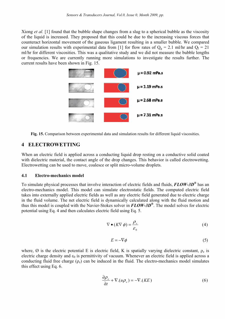
Xiong et al. [1] found that the bubble shape changes from a slug to a spherical bubble as the viscosity of the liquid is increased. They proposed that this could be due to the increasing viscous forces that counteract horizontal movement of the gaseous ligament resulting in a smaller bubble. We compared our simulation results with experimental data from [1] for flow rates of Qg = 2.1 ml/hr and Ql = 21 ml/hr for different viscosities. This was a qualitative study and we did not measure the bubble lengths or frequencies. We are currently running more simulations to investigate the results further. The current results have been shown in Fig. 15.

Fig. 15. Comparison between experimental data and simulation results for different liquid viscosities.

4 ELECTROWETTING

When an electric field is applied across a conducting liquid drop resting on a conductive solid coated with dielectric material, the contact angle of the drop changes. This behavior is called electrowetting. Electrowetting can be used to move, coalesce or split micro-volume droplets.

4.1 Electro-mechanics model

To simulate physical processes that involve interaction of electric fields and fluids, FLOW-3D® has an electro-mechanics model. This model can simulate electrostatic fields. The computed electric field takes into externally applied electric fields as well as any electric field generated due to electric charge in the fluid volume. The net electric field is dynamically calculated along with the fluid motion and thus this model is coupled with the Navier-Stokes solver in FLOW-3D®. The model solves for electric potential using Eq. 4 and then calculates electric field using Eq. 5.

)4()∇(∇0ε

ρφ eK =•

)5(φ−∇=E

where, Ø is the electric potential E is electric field, K is spatially varying dielectric constant, ρe is electric charge density and ε0 is permittivity of vacuum. Whenever an electric field is applied across a conducting fluid free charge (ρe) can be induced in the fluid. The electro-mechanics model simulates this effect using Eq. 6.

)6().().( KEut e

e −∇=∇+∂

∂ ρρ


The model can also take into account force acting on electrically charged fluid volume in the presence of electric field (electrophoresis) and this force (Fe) is calculated using Eq. 7.

)7(EF ee ρ= Another important electric force resulting from gradient in dielectric constant is the dielectrophoresis force (Fd) which is calculated using Eq. 8.

4.2 Electrowetting simulation

We chose an electrowetting case for a hemispherical drop of water (viscosity μ = 0.001 Pa-s, density ρ = 1000 kg/m3). As shown in Fig. 16, the geometry for the simulations consists of a 500 μm diameter hemispherical drop of water placed on a plate coated with a dielectric material having a dielectric constant of 4.5. The static contact angle of the water drop on the coating is 120° and it has an electrical conductivity of 2.5e-5 S/m. A micro-needle electrode is inserted into the top of the drop to apply an electric field across the drop. The steady-state contact angle was measured for the droplet for several voltages from 0 to 25 V.

Fig. 16. Electrowetting simulation setup.

4.3 Results and discussion

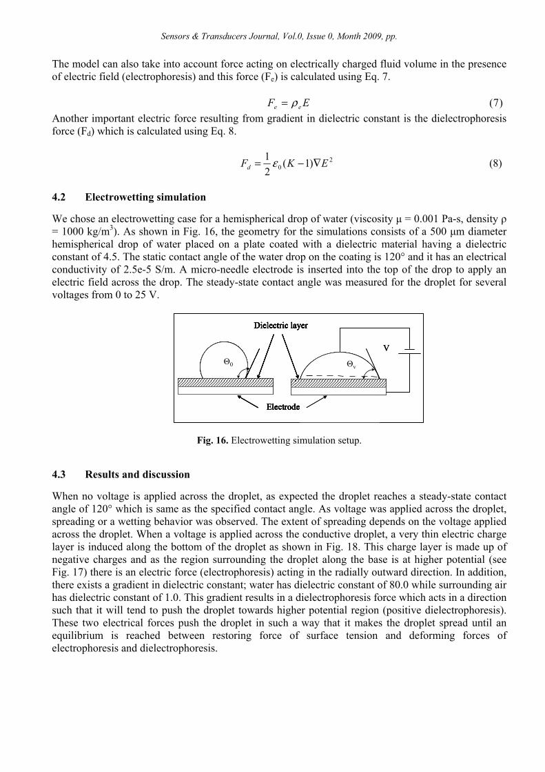
When no voltage is applied across the droplet, as expected the droplet reaches a steady-state contact angle of 120° which is same as the specified contact angle. As voltage was applied across the droplet, spreading or a wetting behavior was observed. The extent of spreading depends on the voltage applied across the droplet. When a voltage is applied across the conductive droplet, a very thin electric charge layer is induced along the bottom of the droplet as shown in Fig. 18. This charge layer is made up of negative charges and as the region surrounding the droplet along the base is at higher potential (see Fig. 17) there is an electric force (electrophoresis) acting in the radially outward direction. In addition, there exists a gradient in dielectric constant; water has dielectric constant of 80.0 while surrounding air has dielectric constant of 1.0. This gradient results in a dielectrophoresis force which acts in a direction such that it will tend to push the droplet towards higher potential region (positive dielectrophoresis). These two electrical forces push the droplet in such a way that it makes the droplet spread until an equilibrium is reached between restoring force of surface tension and deforming forces of electrophoresis and dielectrophoresis.

VΘv

Dielectric layer

Θ0

Electrode

Θv

VΘv

Dielectric layer

Θ0

Electrode

VΘv

Dielectric layer

Θ0

Electrode

Dielectric layer

Θ0

Electrode

Dielectric layer

Θ0

Electrode

Dielectric layer

Θ0

Electrode

Dielectric layer

Θ0

Electrode

Dielectric layer

Θ0Θ0

Electrode

Θv

)8()1(21 2

0 EKFd ∇−= ε


Fig. 17. Comparison of drop shape: a: No electric field, b: 20 V electric field.

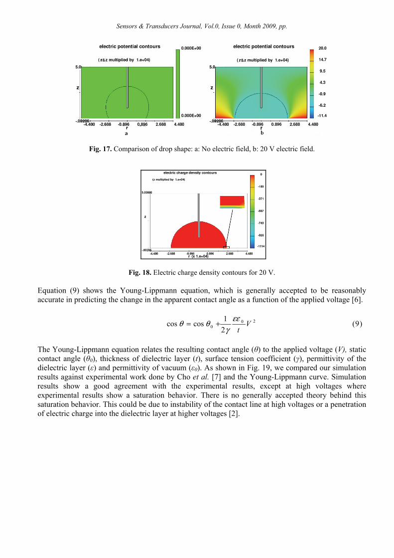
Fig. 18. Electric charge density contours for 20 V. Equation (9) shows the Young-Lippmann equation, which is generally accepted to be reasonably accurate in predicting the change in the apparent contact angle as a function of the applied voltage [6].

)9(21coscos 20

0 Vt

εεγ

θθ +=

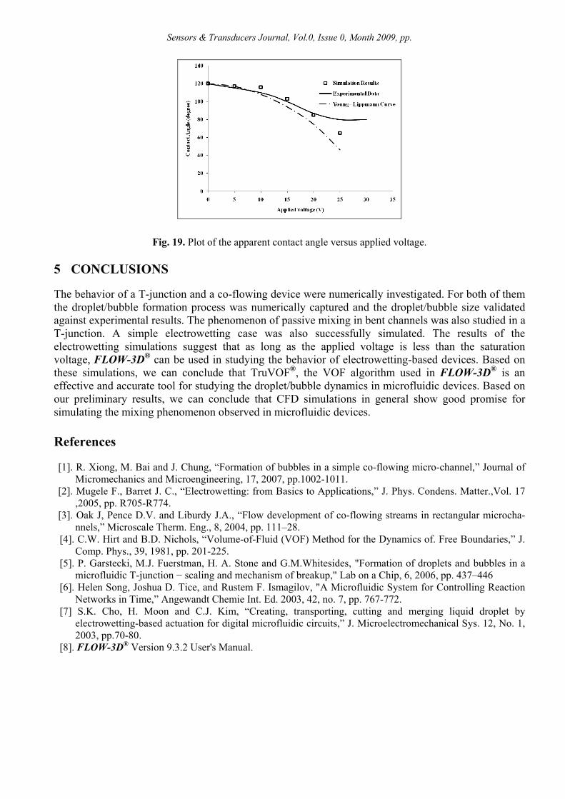
The Young-Lippmann equation relates the resulting contact angle (θ) to the applied voltage (V), static contact angle (θ0), thickness of dielectric layer (t), surface tension coefficient (γ), permittivity of the dielectric layer (ε) and permittivity of vacuum (ε0). As shown in Fig. 19, we compared our simulation results against experimental work done by Cho et al. [7] and the Young-Lippmann curve. Simulation results show a good agreement with the experimental results, except at high voltages where experimental results show a saturation behavior. There is no generally accepted theory behind this saturation behavior. This could be due to instability of the contact line at high voltages or a penetration of electric charge into the dielectric layer at higher voltages [2].


Fig. 19. Plot of the apparent contact angle versus applied voltage.

5 CONCLUSIONS

The behavior of a T-junction and a co-flowing device were numerically investigated. For both of them the droplet/bubble formation process was numerically captured and the droplet/bubble size validated against experimental results. The phenomenon of passive mixing in bent channels was also studied in a T-junction. A simple electrowetting case was also successfully simulated. The results of the electrowetting simulations suggest that as long as the applied voltage is less than the saturation voltage, FLOW-3D® can be used in studying the behavior of electrowetting-based devices. Based on these simulations, we can conclude that TruVOF®, the VOF algorithm used in FLOW-3D® is an effective and accurate tool for studying the droplet/bubble dynamics in microfluidic devices. Based on our preliminary results, we can conclude that CFD simulations in general show good promise for simulating the mixing phenomenon observed in microfluidic devices. References [1]. R. Xiong, M. Bai and J. Chung, “Formation of bubbles in a simple co-flowing micro-channel,” Journal of

Micromechanics and Microengineering, 17, 2007, pp.1002-1011. [2]. Mugele F., Barret J. C., “Electrowetting: from Basics to Applications,” J. Phys. Condens. Matter.,Vol. 17

,2005, pp. R705-R774. [3]. Oak J, Pence D.V. and Liburdy J.A., “Flow development of co-flowing streams in rectangular microcha-

nnels,” Microscale Therm. Eng., 8, 2004, pp. 111–28. [4]. C.W. Hirt and B.D. Nichols, “Volume-of-Fluid (VOF) Method for the Dynamics of. Free Boundaries,” J.

Comp. Phys., 39, 1981, pp. 201-225. [5]. P. Garstecki, M.J. Fuerstman, H. A. Stone and G.M.Whitesides, "Formation of droplets and bubbles in a

microfluidic T-junction − scaling and mechanism of breakup," Lab on a Chip, 6, 2006, pp. 437–446 [6]. Helen Song, Joshua D. Tice, and Rustem F. Ismagilov, "A Microfluidic System for Controlling Reaction

Networks in Time,” Angewandt Chemie Int. Ed. 2003, 42, no. 7, pp. 767-772. [7] S.K. Cho, H. Moon and C.J. Kim, “Creating, transporting, cutting and merging liquid droplet by

electrowetting-based actuation for digital microfluidic circuits,” J. Microelectromechanical Sys. 12, No. 1, 2003, pp.70-80.

[8]. FLOW-3D® Version 9.3.2 User's Manual.

Simulation of Droplet Dynamics and Mixing in … of Droplet Dynamics and Mixing in ... is an...

Documents

Transcript of Simulation of Droplet Dynamics and Mixing in … of Droplet Dynamics and Mixing in ... is an...