Simulation of Cracks in a Cosserat

Medium using the eXtended Finite

Element Method

by

Maria Kapiturova

A thesis

presented to the University of Waterloo

in fulfillment of the

thesis requirement for the degree of

Master of Applied Science

in

Civil Engineering

Waterloo, Ontario, Canada, 2013

c© Maria Kapiturova 2013

Author’s Declaration

I hereby declare that I am the sole author of this thesis. This is a true copy of the thesis,

including any required final revisions, as accepted by my examiners.

I understand that my thesis may be made electronically available to the public.

ii

Abstract

This research investigates fracture behaviour in the Cosserat materials. The Cosserat

elasticity description of the materials incorporates a characteristic length scale (e.g. grains,

particles, fibres, etc.) into the model. The characteristic length scale in such materials is

known to significantly influence the macroscopic behaviour of the whole body. Simulation

of the fracture processes, such as crack opening and propagation, in Cosserat materials still

remains a challenge for the scientific community. The goal of this thesis is to propose and

validate a two dimensional extended finite element method model of edge cracks within

the Cosserat elasticity theory framework.

The crack modelling was conducted using the Finite Element Method (FEM) and eX-

tended Finite Element Method (XFEM) implemented in the Matlab code. The strong and

weak formulations of the problem and the discrete XFEM equations are presented in the

thesis. Mode I and II edge crack models in a Cosserat medium are discussed and verified

through a series of patch and convergence tests. In addition, the numerical evaluation of

the J-integral for the Cosserat medium is presented, and the J-integral for the Cosserat

medium is compared to the J-integral for the classical elasticity.

The XFEM/Cosserat method is shown to be robust and able to effectively model the

edge crack problems in a Cosserat medium. Moreover, the elastic parameter α is found to

be a powerful coupling tool between the microrotations and the translations. The Cosserat

J-integral differs from the classical J-integral by 2% to 40%, for a given crack depending

on the micropolar elastic coupling constant α.

iii

Acknowledgements

I would like to thank my supervisors, Dr. Robert Gracie and Dr. Stanislav Potapenko,

for their guidance and support during my study at the University of Waterloo.

I would like to thank my mom, my grand mom, my brother and his family for their

enormous love, care and encouragement.

I would like to thank my dear friends for being supportive and providing warm envi-

ronment during these two years.

iv

Dedication

This thesis is dedicated to my parents, Roman Kapiturov and Svetlana Kapiturova.

v

Table of Contents

List of Tables ix

List of Figures x

1 Introduction 1

1.1 Background . . . . . . . . . . . . . . . . . . . . . . . . . . . . . . . . . . . 1

1.2 Scope and objectives . . . . . . . . . . . . . . . . . . . . . . . . . . . . . . 2

1.3 Organization of the thesis . . . . . . . . . . . . . . . . . . . . . . . . . . . 3

2 Literature Review 5

2.1 Cosserat continuum . . . . . . . . . . . . . . . . . . . . . . . . . . . . . . . 5

2.1.1 Cosserat materials . . . . . . . . . . . . . . . . . . . . . . . . . . . 5

2.1.2 Development of the Cosserat theory of elasticity . . . . . . . . . . . 9

2.1.3 Description of the Cosserat model . . . . . . . . . . . . . . . . . . . 12

2.2 Modelling of discontinuities . . . . . . . . . . . . . . . . . . . . . . . . . . 16

2.2.1 Existing models of discontinuities . . . . . . . . . . . . . . . . . . . 16

2.2.2 Methods of numerical modelling of cracks . . . . . . . . . . . . . . 18

2.3 Linear elastic fracture mechanics . . . . . . . . . . . . . . . . . . . . . . . 20

vi

2.3.1 Fracture mechanics in the classical theory of elasticity . . . . . . . . 20

2.3.2 Fracture mechanics in the Cosserat theory of elasticity . . . . . . . 24

2.4 Cosserat models coupled with the Finite Element Method . . . . . . . . . . 28

2.5 Cosserat models coupled with the eXtended Finite Element Method . . . . 30

3 Overview of the FEM 32

3.1 Overview . . . . . . . . . . . . . . . . . . . . . . . . . . . . . . . . . . . . . 32

3.2 Shape functions construction . . . . . . . . . . . . . . . . . . . . . . . . . . 33

3.3 Gauss quadrature . . . . . . . . . . . . . . . . . . . . . . . . . . . . . . . . 37

3.4 Convergence of FEM . . . . . . . . . . . . . . . . . . . . . . . . . . . . . . 38

3.4.1 Errors in the approximation . . . . . . . . . . . . . . . . . . . . . . 38

3.4.2 Measures of the errors . . . . . . . . . . . . . . . . . . . . . . . . . 38

3.4.3 Accuracy of the solution . . . . . . . . . . . . . . . . . . . . . . . . 39

3.5 Verification of FEM . . . . . . . . . . . . . . . . . . . . . . . . . . . . . . . 40

3.5.1 Computation scheme for the error evaluation of the XFEM solution

with the FEM exact solution . . . . . . . . . . . . . . . . . . . . . . 41

4 XFEM Model of the Crack in the Cosserat Elastic Material 43

4.1 Governing equations . . . . . . . . . . . . . . . . . . . . . . . . . . . . . . 43

4.2 Weak form . . . . . . . . . . . . . . . . . . . . . . . . . . . . . . . . . . . . 46

4.3 Discrete equations . . . . . . . . . . . . . . . . . . . . . . . . . . . . . . . . 46

4.4 Numerical integration . . . . . . . . . . . . . . . . . . . . . . . . . . . . . . 52

4.5 Crack opening model . . . . . . . . . . . . . . . . . . . . . . . . . . . . . . 56

4.6 Computation scheme of the J-integral evaluation . . . . . . . . . . . . . . . 57

vii

5 Numerical Examples 58

5.1 Introduction . . . . . . . . . . . . . . . . . . . . . . . . . . . . . . . . . . . 58

5.2 Convergence study of the FEM/Cosserat solution for the domain without a

crack with α 6= 0 . . . . . . . . . . . . . . . . . . . . . . . . . . . . . . . . 59

5.3 Convergence study of the XFEM/Cosserat solution of the edge crack prob-

lem in the domain with the prescribed analytical solution on the boundaries

with α = 0 . . . . . . . . . . . . . . . . . . . . . . . . . . . . . . . . . . . . 61

5.4 Convergence study of the XFEM/Cosserat solution of the edge crack prob-

lem with α 6= 0 . . . . . . . . . . . . . . . . . . . . . . . . . . . . . . . . . 67

5.4.1 Mode I edge crack . . . . . . . . . . . . . . . . . . . . . . . . . . . 67

5.4.2 Mode II edge crack . . . . . . . . . . . . . . . . . . . . . . . . . . . 70

5.5 Calculation of the J-integral in a Cosserat medium . . . . . . . . . . . . . 72

5.5.1 Verification of the J-integral calculation . . . . . . . . . . . . . . . . 72

5.5.2 Comparison of the J-integral for the Cosserat elastic medium and

classical elastic medium . . . . . . . . . . . . . . . . . . . . . . . . 76

6 Conclusions and Recommendations 80

6.1 Concluding remarks . . . . . . . . . . . . . . . . . . . . . . . . . . . . . . . 80

6.2 Recommendations for the future development . . . . . . . . . . . . . . . . 81

APPENDICES 83

A Matrix definitions 84

References 90

viii

List of Tables

3.1 Nodal coordinates in the parametric element domain. . . . . . . . . . . . . 36

ix

List of Figures

2.1 Cosserat materials: (a) layered rock (ipb.ac.rs), (b) rock mass (qusterre.com),

(c) porous concrete ( soa.utexas.edu). . . . . . . . . . . . . . . . . . . . . . 7

2.2 Cosserat materials: (a) polymer (sbio.uct.ac.za), (b) composite (fz-juelich.de),

(c) cellular solid (web.mit.edu), (d) bone (mhhe.com). . . . . . . . . . . . . 8

2.3 The representation of the degrees of freedom in the Cosserat model. . . . . 12

2.4 Representation of the force balance in (a) classical elasticity, and (b) Cosserat

elasticity. . . . . . . . . . . . . . . . . . . . . . . . . . . . . . . . . . . . . 13

2.5 Moment equilibrium in 2D. . . . . . . . . . . . . . . . . . . . . . . . . . . . 15

2.6 Weak discontinuities: (a) material interface (materialinterface.com), (b) in-

clusion (skywalker.cochise.edu). . . . . . . . . . . . . . . . . . . . . . . . . 17

2.7 Strong discontinuities: (a) crack (msnbc.msn.com), (b) dislocation (Loudet

J.C. et al., 2001). . . . . . . . . . . . . . . . . . . . . . . . . . . . . . . . . 17

2.8 Representation of the coordinate systems: (x1, x2) - global coordinates,

(x1, x2) - local crack coordinates, (r, θ) - polar coordinates. . . . . . . . . . 21

2.9 The representation of distribution of KI

KIas a function of α

E, parametrized by

γ (Diegele et al., 2004). . . . . . . . . . . . . . . . . . . . . . . . . . . . . . 26

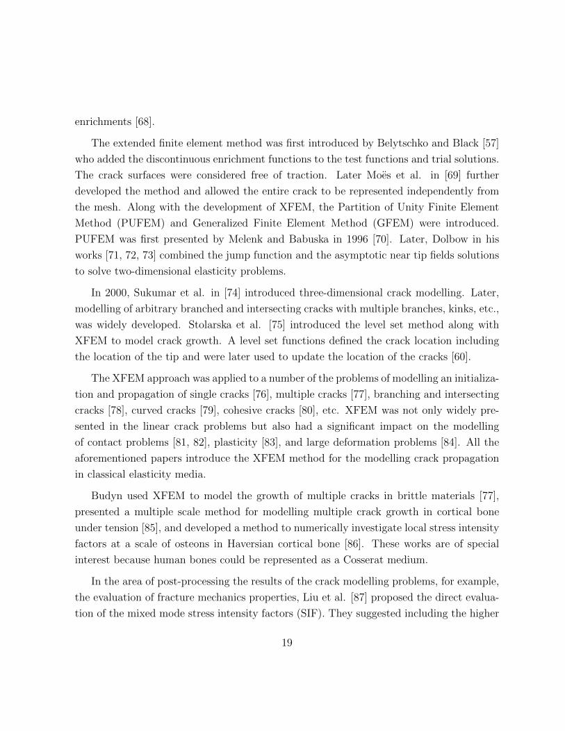
2.10 The representation of distribution of LI as a function of αE

, parametrized by

γ (Diegele et al., 2004). . . . . . . . . . . . . . . . . . . . . . . . . . . . . . 27

3.1 The representation of the shape functions for the two-node element. . . . . 33

x

3.2 The representation of the shape functions for the rectangular element in 2D. 35

3.3 Mapping from the parent coordinates to the physical coordinates (Fish,

Belytschko. A First Course in Finite Elements). . . . . . . . . . . . . . . . 36

4.1 Body with external and internal boundaries subjected to loads. . . . . . . . 44

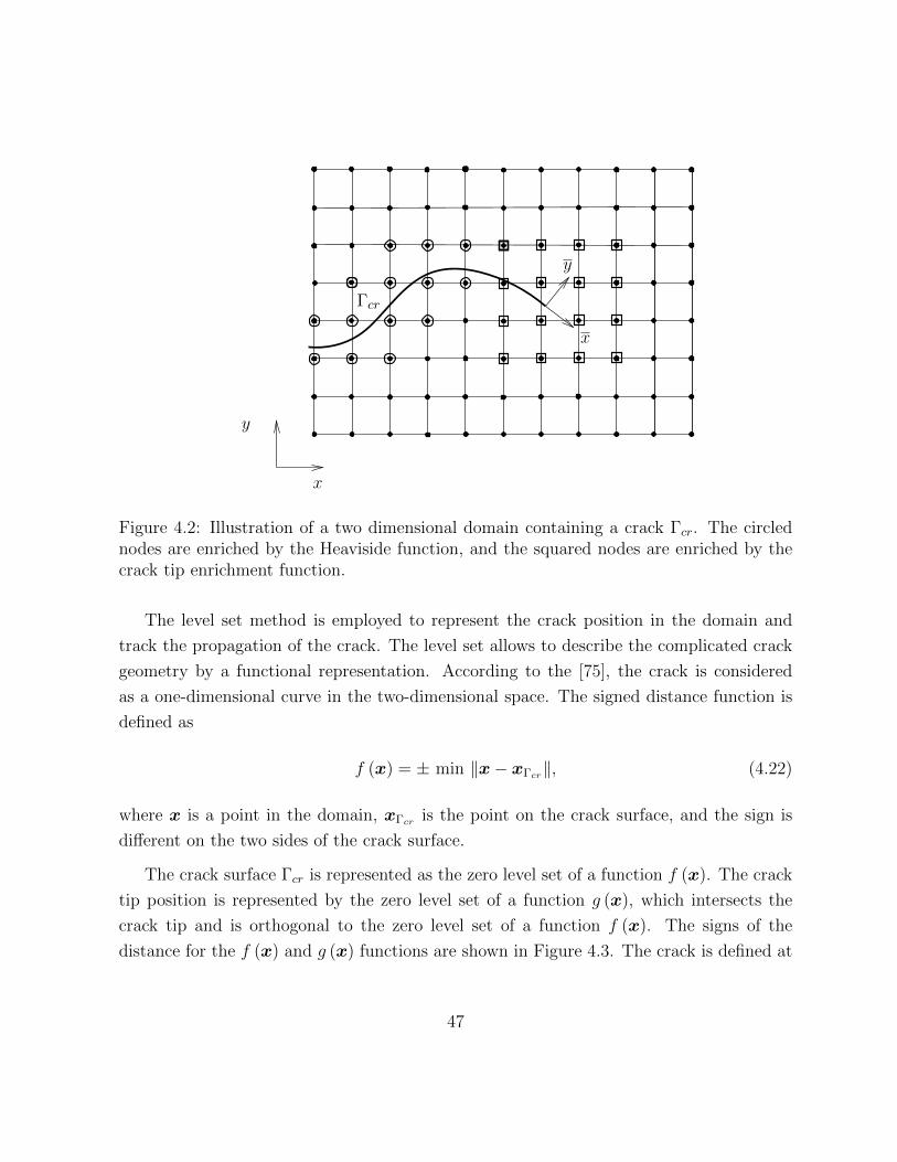
4.2 Illustration of a two dimensional domain containing a crack Γcr. The circled

nodes are enriched by the Heaviside function, and the squared nodes are

enriched by the crack tip enrichment function. . . . . . . . . . . . . . . . . 47

4.3 Level set method for the crack growth modelling. . . . . . . . . . . . . . . 48

4.4 The representation of the Gauss quadrature rule in the element containing

crack tip. . . . . . . . . . . . . . . . . . . . . . . . . . . . . . . . . . . . . 53

4.5 Selected elements for the geometrical enrichment with the number of ele-

ments: (a) 11×11, (b) 51×51. . . . . . . . . . . . . . . . . . . . . . . . . . 54

4.6 Selected elements for the topological enrichment with the number of ele-

ments: (a) 11×11, (b) 51×51. . . . . . . . . . . . . . . . . . . . . . . . . . 55

5.1 The square domain without a crack. . . . . . . . . . . . . . . . . . . . . . . 59

5.2 Convergence rates of the FEM solutions for the α=0, 100, 1000. . . . . . . 60

5.3 Edge crack in a finite domain. . . . . . . . . . . . . . . . . . . . . . . . . . 61

5.4 Convergence study of the Mode I edge crack problem in a Cosserat medium

with α = 0. . . . . . . . . . . . . . . . . . . . . . . . . . . . . . . . . . . . 63

5.5 Convergence study for the coupled Mode I edge crack case solved by XFEM

with topological tip enrichment with varying number of enriched nodes layers

from 1 to 4. . . . . . . . . . . . . . . . . . . . . . . . . . . . . . . . . . . . 65

5.6 Convergence study for the coupled Mode I edge crack case solved by XFEM

with geometrical tip enrichment with varying radius from L/5 to L/20. . . 66

5.7 The domain with an edge crack under tension. . . . . . . . . . . . . . . . . 67

xi

5.8 Convergence rates of the XFEM solutions of the edge crack problem under

the tension loading with α=1000. . . . . . . . . . . . . . . . . . . . . . . . 69

5.9 The square domain with an edge crack under shear loading. . . . . . . . . 70

5.10 Convergence rates of the FEM solutions of the edge crack problem under

the shear loading for the α=1000. . . . . . . . . . . . . . . . . . . . . . . . 71

5.11 The domain with an edge crack. The asymptotic field solutions are pre-

scribed on the boundaries. . . . . . . . . . . . . . . . . . . . . . . . . . . . 72

5.12 The representation of the J-integral dependence on the contour radius. . . 73

5.13 The representation of dependence of J-integral from KI with LI = 0. . . . 75

5.14 The domain with an edge crack under shear. . . . . . . . . . . . . . . . . . 76

5.15 The J-integral versus the crack length. . . . . . . . . . . . . . . . . . . . . 78

5.16 The normalized J-integral with respect to the crack length. . . . . . . . . . 79

xii

Chapter 1

Introduction

1.1 Background

The classical linear theory of elasticity began developing in 1820, based on the original

works of Cauchy and Navier [1, 2]. The theory deals with the elastic deformations of solid

materials and has numerous applications in engineering. In 1880-1890, Voigt and Duhem

made the first attempts to generalize the conventional theory of elasticity by introducing

an independent moment vector and polar medium, where the stress tensor is not symmet-

ric. The first complete theory based on these assumptions was presented by the Cosserat

brothers in 1909 and was named Cosserat theory of elasticity. Unfortunately, the proposed

theory was not widely accepted by the scientific society due to its unclear formulation and

generality (the theory considered the problems of fluid mechanics, electrodynamics and

magnetism, in addition to the elasticity problems). However, in 1970-1980, with the inven-

tion and development of new materials, such as composites, polymers, etc., the Cosserat

theory was reconsidered. A large number of experimental and theoretical studies have

shown that the behaviour of some materials cannot be described by the classical elastic-

ity explicitly. The studies of Roderic Lakes in 1980s’ have had a significant impact on

the development and understanding of the Cosserat theory. In his works, he classified

human and bovine bones as a Cosserat material, conducted experimental research on the

Cosserat elastic parameters, and proved the advantages of the Cosserat theory over the

1

classical theory for describing the materials with a complex microstructure. Later, the in-

vention of such powerful technique as the Finite Element Method (FEM) made it possible

to conduct the numerical modelling of Cosserat materials behaviour, although mostly in

the geomechanical area [3, 4, 5, 6].

The Cosserat model is classified as a generalized continuum model, having additional

degrees of freedom (also called higher-order continuum model). Therefore, the model can

be used for a research of numerous recently developed materials. For example, Cosserat

medium may be considered as a model for granular materials, describing the development

of shear bands with the help of rotational degrees of freedom. It can also be considered as

a homogenized continuum for discrete and layered materials, and materials with periodic

or random microstructures. Also, the Cosserat theory may predict size-effect in bone-like

structures and cellular media. There is a big potential for research in the area of modelling

materials with complex microstructure behaviour using the Cosserat theory of elasticity.

In this research, the Cosserat theory of elasticity is considered as a new and promising

way to describe fracture processes such as crack opening in a Cosserat medium. However,

there are a few challenges in the fracture analysis of Cosserat materials due to a lack of

studies of fracture parameters such as stress intensity factors and their relations with the

J-integral.

1.2 Scope and objectives

The scope of this thesis is to develop an effective fracture model in a Cosserat elastic

medium. The numerical tools used for the research are the Finite Element Method and the

eXtended Finite Element Method. Matlab was used as a numerical computing environment

to model crack opening problems. The XFEM/Cosserat model was verified by comparing

the obtained numerical solution with the known analytical solution and the exact FEM

solution, as well as by conducting convergence studies.

The objectives of the thesis are to:

• conduct a literature review to understand the Cosserat elasticity theory, fracture

mechanics concepts, and numerical methods used in the research;

2

• describe the Cosserat model, the derivation of the strong and weak forms, and the

discrete equations for the numerical methods;

• provide examples showing the verification, convergence and effectiveness of the model;

• present the verified calculation of the J-integral for Cosserat solids;

• compare the J-integral for Cosserat elastic solid and classical elastic solid;

• show the dependence of the Cosserat J-integral on the crack sizes; and

• discuss the results of fracture modelling in Cosserat media, giving further recommen-

dation for the development and proposing the possible practical applications of the

model.

1.3 Organization of the thesis

Chapter 2 provides an introduction and a literature review of the Cosserat elasticity theory

and the history of its development. The concepts of Linear Elastic Fracture Mechanics for

the classical and Cosserat elasticity theories are described. The types of discontinuities and

numerical methods for the modelling are overviewed. The existing papers on the Cosserat

problems solved by the Finite Element Method and the eXtended Finite Element Method

are discussed.

Chapter 3 gives an overview of the Finite Element Method formulation. The construc-

tion of approximations and trial solutions are presented. The error estimation method is

discussed.

Chapter 4 describes the eXtended Finite Element Method model of the crack opening

problem in a Cosserat medium. The strong and weak forms of the problem are stated.

The derivation of the governing equations and the discrete equations are presented. Nu-

merical integration scheme, the algorithm of the crack opening problem, and the J-integral

computation scheme are described.

3

Chapter 5 presents the numerical modelling of the fracture processes in a Cosserat

material: the crack opening problems, the verification and convergence tests, and the

discussion of the obtained results. In addition, the numerical evaluation of J-integral is

presented.

Chapter 6 constitutes the conclusion of the research project and offers the recommen-

dations for the future development of the topic.

4

Chapter 2

Literature Review

This section describes the historical perspective and provides an up-to-date overview of

the Cosserat theory. The current methods of modelling discontinuities in classical and

Cosserat materials are presented.

2.1 Cosserat continuum

2.1.1 Cosserat materials

A number of modern materials have complex microstructures, which generally involve

characteristic length scales. Examples of the characteristic length scales are grains, par-

ticles, fibres, cells, etc. [7]. Conventional classical continuum mechanics approaches do

not incorporate the effect of the intrinsic length into the models, whereas the description

of such materials as a Cosserat continuum takes that effect into account. The Cosserat

theory of elasticity was developed in the beginning of the twentieth century and is also

known as the micropolar theory of elasticity [8, 9, 10]. Numerous experiments conducted

by the researchers in the 1970s and 1980s [11, 12, 13] showed that the Cosserat theory of

elasticity described the mechanical behaviour of the materials with characteristic length

scales explicitly, while the classical theory of elasticity was not capable of doing so. Due

5

to these observations, the Cosserat theory became especially interesting for the researchers

who were developing advanced technologies and materials. For example, these materials

are carbon-fibre-reinforced composite materials that are used in aerospace components and

in spacecraft construction [14], porous concrete used in civil engineering [15], orthopaedic

implants used in biomechanics [16], etc.

The examples of the materials that could be described by the Cosserat theory of elas-

ticity are presented in Figures 2.1 and 2.2. The characteristic microstructure can be easily

recognized for each of the shown materials.

6

(a) (b)

(c)

Figure 2.1: Cosserat materials: (a) layered rock (ipb.ac.rs), (b) rock mass (qusterre.com),(c) porous concrete ( soa.utexas.edu).

7

(a) (b)

(c) (d)

Figure 2.2: Cosserat materials: (a) polymer (sbio.uct.ac.za), (b) composite (fz-juelich.de),(c) cellular solid (web.mit.edu), (d) bone (mhhe.com).

8

2.1.2 Development of the Cosserat theory of elasticity

Since the classical theory of elasticity [17] was not able to accurately describe the mechan-

ical behaviour of the materials with complex microstructures, the new extended theory of

elasticity began to be considered by scientists. In 1886, Voigt described the medium where

an independent moment vector, in addition to a conventional force vector, was introduced

to transfer the loading through the surface of the body [18]. According to this assumption,

the stress and strain tensors were asymmetric. Then, in 1893, Duhem suggested that the

materials could be visualized and described as the sets of points having vectors attached

to them, named oriented or polar medium [19].

Later, the first complete extended elasticity theory based on Voigt’s assumptions was in-

troduced by the brothers Francois and Eugene Cosserat in 1909 [9]. The authors described

the material transformation by translations (displacements) and infinitesimal microrota-

tions at each point of the body. They also derived the equations of balance of forces and

balance of angular momentum. The Cosserat brothers created a unified theory to describe

solid and fluid mechanics, elastodynamics, and magnetism; however, that theory was too

sophisticated for that time. The simplified Cosserat theory with the constrained microrota-

tions was suggested by Truesdell and Toupin in [20, 21], and, later, described by Kupradze

in [22]. The name of the developed theory with constrained rotations was the couple stress

theory or Cosserat pseudo continuum theory. The rotation vector was dependent on the

displacement vector; therefore, the deformation of the body was described solely by the

conventional displacement field. However, the stress tensor remained asymmetric so that

the equilibrium with the generating couple stresses was preserved. Meanwhile, the research

on the Cosserat theory with the independent rotations was conducted by Gunter [23] and

Shaefer [24, 25], Aero and Kuvshinsky [26], and Palmov [27].

Eringen further developed the Cosserat theory of elasticity in 1966. He showed that

the classical theory of elasticity and the couple stress theory are the special cases of the

Cosserat elasticity theory [8, 28]. At the same time, a full description of the Cosserat

theory was presented by Nowacki in [10]. In his works, Nowacki introduced the broad

description of the static problems of asymmetric elasticity, problems of thermoelasticity

and thermopiezoelectricity in a micropolar medium. The Cosserat medium descriptions of

9

Eringen and Nowacki differ insignificantly in terms of Cosserat elastic constants presented

in the governing equations and constitutive relations.

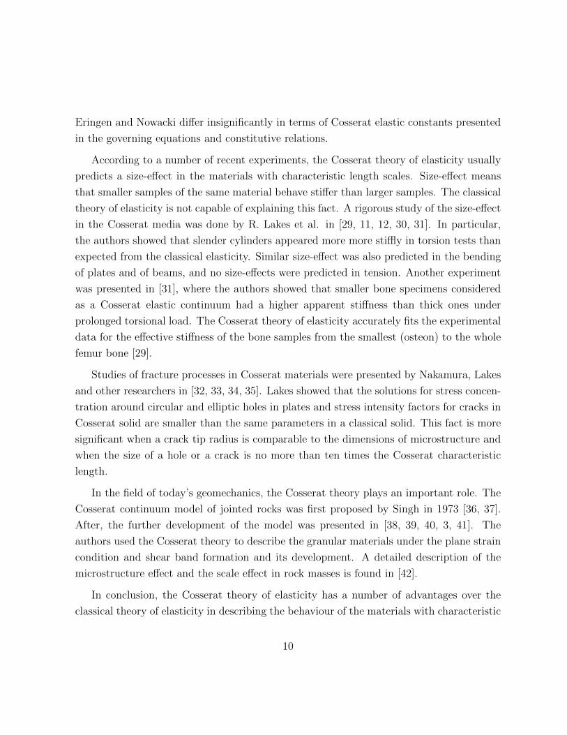
According to a number of recent experiments, the Cosserat theory of elasticity usually

predicts a size-effect in the materials with characteristic length scales. Size-effect means

that smaller samples of the same material behave stiffer than larger samples. The classical

theory of elasticity is not capable of explaining this fact. A rigorous study of the size-effect

in the Cosserat media was done by R. Lakes et al. in [29, 11, 12, 30, 31]. In particular,

the authors showed that slender cylinders appeared more more stiffly in torsion tests than

expected from the classical elasticity. Similar size-effect was also predicted in the bending

of plates and of beams, and no size-effects were predicted in tension. Another experiment

was presented in [31], where the authors showed that smaller bone specimens considered

as a Cosserat elastic continuum had a higher apparent stiffness than thick ones under

prolonged torsional load. The Cosserat theory of elasticity accurately fits the experimental

data for the effective stiffness of the bone samples from the smallest (osteon) to the whole

femur bone [29].

Studies of fracture processes in Cosserat materials were presented by Nakamura, Lakes

and other researchers in [32, 33, 34, 35]. Lakes showed that the solutions for stress concen-

tration around circular and elliptic holes in plates and stress intensity factors for cracks in

Cosserat solid are smaller than the same parameters in a classical solid. This fact is more

significant when a crack tip radius is comparable to the dimensions of microstructure and

when the size of a hole or a crack is no more than ten times the Cosserat characteristic

length.

In the field of today’s geomechanics, the Cosserat theory plays an important role. The

Cosserat continuum model of jointed rocks was first proposed by Singh in 1973 [36, 37].

After, the further development of the model was presented in [38, 39, 40, 3, 41]. The

authors used the Cosserat theory to describe the granular materials under the plane strain

condition and shear band formation and its development. A detailed description of the

microstructure effect and the scale effect in rock masses is found in [42].

In conclusion, the Cosserat theory of elasticity has a number of advantages over the

classical theory of elasticity in describing the behaviour of the materials with characteristic

10

length scales. A good summary of general applications of the Cosserat theory is found in

[43, 44]. The Cosserat theory of elasticity may be a replacement for a granular assembly,

masonry or blocky structures, where the particle rotations are known to be important in

the development of shear bands. In geomechanics, this ability allows to get a large-scale

response of the media. The Cosserat theory also allows researchers to homogenize continua

for the discrete structural elements and media with periodic and random microstructure.

In addition, the Cosserat theory is capable of predicting size-effect in particular mechan-

ical tests (bending and torsion) and of describing the fracture behaviour of the foam-like

structures more accurately.

11

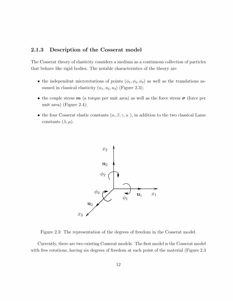
2.1.3 Description of the Cosserat model

The Cosserat theory of elasticity considers a medium as a continuous collection of particles

that behave like rigid bodies. The notable characteristics of the theory are

• the independent microrotations of points (φ1, φ2, φ3) as well as the translations as-

sumed in classical elasticity (u1, u2, u3) (Figure 2.3);

• the couple stress m (a torque per unit area) as well as the force stress σ (force per

unit area) (Figure 2.4);

• the four Cosserat elastic constants (α, β, γ, κ ), in addition to the two classical Lame

constants (λ, µ).

u1

u3

u2

x2

φ2

x1

x3

φ3φ1

Figure 2.3: The representation of the degrees of freedom in the Cosserat model.

Currently, there are two existing Cosserat models. The first model is the Cosserat model

with free rotations, having six degrees of freedom at each point of the material (Figure 2.3

12

tmtσ

bm

bσ

x1

x2

x3

tσ

bσ

(a)

tm

tσ

bmbσ

x1

x2

x3

(b)

Figure 2.4: Representation of the force balance in (a) classical elasticity, and (b) Cosseratelasticity.

[45]). The second model is the Cosserat model with constrained rotations, where particles

have only three conventional degrees of freedom (translations). Although the stress tensor

is not symmetric, as it is in the first model, the couple stresses are presented to satisfy

equilibrium [26]. The Cosserat model with free rotations is described below in detail and

is used in this research.

In order for the specific internal energy function to remain positive, the Cosserat ma-

terial parameters must obey the following inequalities [45]:

3λ+ 2µ ≥ 0, µ ≥ 0, α ≥ 0,

3β + 2γ ≥ 0, γ ≥ 0, κ ≥ 0. (2.1)

An important characteristic for Cosserat media is the coupling number N , which ranges

in value from 0 (classical elasticity theory, corresponds to κ = 0) to 1 (indeterminate couple

stress theory, corresponds to κ→∞) [46]:

N =

(κ

2 (µ+ κ)

)1/2

=

(κ (1 + ν)

E + κ (1 + ν)

)1/2

(2.2)

13

The original technical elasticity constants could be expressed through the Cosserat

elastic constants [8, 47]:

Young’s modulus E =(2µ+ κ) (2λ+ 2µ+ κ)

(2λ+ 2µ+ κ), (2.3)

Shear modulus G =(2µ+ κ)

2, (2.4)

Poisson’s ratio ν =λ

(2λ+ 2µ+ κ). (2.5)

Materials with complex microstructures (granular, fibrous, porous, etc.) have a number

of intrinsic length scales. In the two-dimensional context, the internal length scale is

identified as the characteristic length for bending or torsion that is defined through the

material constants [30]. The characteristic length for bending is

lb =

(γ

2µ+ 2κ

)1/2

=

(γ (1 + ν)

2E

)1/2

(2.6)

and for torsion is

lt =

(β + γ

2µ+ κ

)1/2

. (2.7)

In the classical solids, the internal characteristic length scale is of the order of the

atomic distance; therefore, couple forces do not produce any macroscopic effect. However,

in the Cosserat materials, the characteristic length scale is of the order of microns, and

couple stresses may influence the mechanical behaviour of the whole body. For instance,

the characteristic length scale for steel is 0.05 mm; for bone, 1 mm; and for masonry or

rock masses, 100 mm [7].

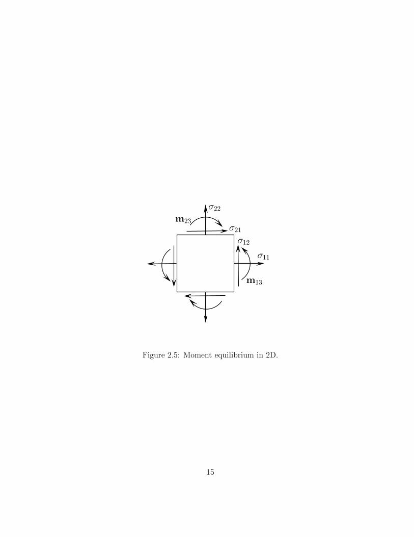
One of the essential features of the Cosserat continuum is that the stress tensor is not

symmetric, and asymmetric shear stresses are equilibrated by the couple stresses (Fig-

ure 2.5).

14

σ22

σ11

σ21σ12

m13

m23

Figure 2.5: Moment equilibrium in 2D.

15

2.2 Modelling of discontinuities

This section presents an overview of the types and models of discontinuities, as well as the

description of the numerical methods of modelling.

2.2.1 Existing models of discontinuities

There are two main types of discontinuities:

• weak - the displacement field remains continuous, and the strain field may or may

not be continuous;

• strong - both the displacement and strain fields are discontinuous.

Weak discontinuities are mainly continuous problems such as material interfaces and

inclusions (Figure 2.6), and strong discontinuities are cracks, dislocations, and voids (Fig-

ure 2.7).

In the current research, the crack opening in a Cosserat medium is modelled based on

the concepts of fracture mechanics and the extended finite element method. In general,

crack simulation may be described by the non-local model [48], the continuous smeared

crack model [49], the discrete crack model [50], etc.

Non-local models allow researchers to avoid mesh dependency for the simulation of the

crack propagation [51]. The model assumes that the fracture behaviour of each point is

affected by the stress state at that point and a number of surrounding points. The smeared

crack model simulates the mechanics of the crack in terms of stiffness and strength reduc-

tion instead of the geometrical modelling of the crack. However, the smeared crack model

does not require remeshing while the crack propagates only in the case of the predefined

crack path. In the discrete crack model, the discontinuity is defined along the finite element

edges or along the sub-mesh inside the elements. Subsequently, the method is expensive

and time-consuming because of remeshing. In this research, the discrete crack model is

used at one of the stages to simulate crack opening using the Finite Element Method.

16

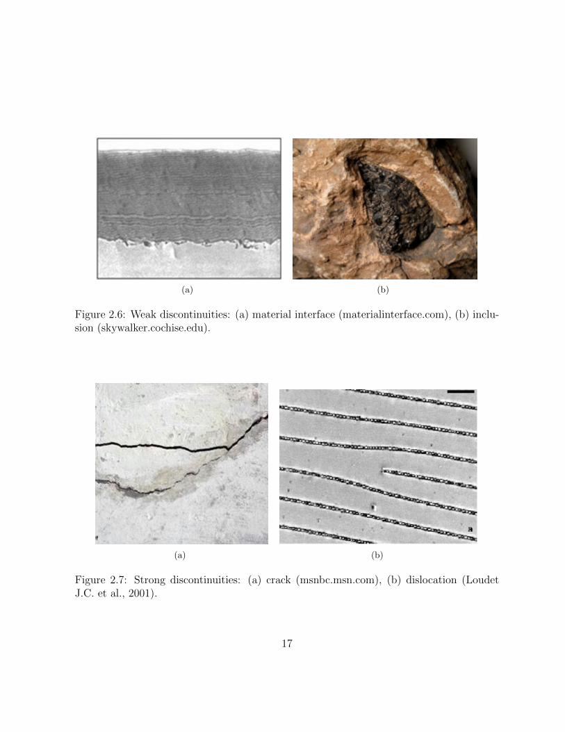
(a) (b)

Figure 2.6: Weak discontinuities: (a) material interface (materialinterface.com), (b) inclu-sion (skywalker.cochise.edu).

(a) (b)

Figure 2.7: Strong discontinuities: (a) crack (msnbc.msn.com), (b) dislocation (LoudetJ.C. et al., 2001).

17

2.2.2 Methods of numerical modelling of cracks

A number of methods for the simulation of the opening and propagation of cracks exist

[51]: analytical, semi-analytical, and numerical approaches that have been developed in

the past years. Numerical methods include the boundary integral method [52, 53], the

boundary element method [54, 55], the finite element method [56], the extended finite

element method [57], the discrete element based method [58], and the meshless method

[59].

The basis of the boundary integral method (BIM) is the development of a boundary

constraint equation that relates all boundary displacements to all boundary tractions. Both

the boundary integral method and the boundary element method (BEM) are restricted to

the particular types of problems to which boundary elements can be applied usefully. These

are problems with a small surface-volume ratio. However, for many engineering problems,

the BEM and BIM are significantly less efficient than the methods such as finite element

method. In contrast, the most attractive feature of FEM is its ability to model complicated

geometries and boundaries. The finite element method is a powerful numerical tool for the

analysis of engineering and physical problems.

The problem of crack modelling in a micropolar medium that is solved in this research

is based on the extended finite element method. The method has been already successfully

applied for the modelling of different kinds of discontinuities in solids such as cracks [60],

interfaces [61], inclusions [62], dislocations [63, 64, 65, 66], etc. The XFEM is a numerical

method to model internal (or external) boundaries without requiring the mesh to conform

to the boundaries. The technique allows modelling the entire crack geometry independently

of the mesh and avoiding the need to re-mesh while the crack propagates. The main

idea is to introduce special enrichment functions (for instance, Heaviside function, branch

functions, etc.) that depend on the nature of the discontinuity into the standard finite

element approximation. Hansbo and Hansbo [67] developed a slightly different method:

the phantom node method. This method is based on doubling nodes for every element that

is crossed by a discontinuity. The deformation field is interpolated independently on both

sides of the discontinuity. The difference between the phantom node method and XFEM

lies only in the implementation; however, XFEM is more compatible with the singularity

18

enrichments [68].

The extended finite element method was first introduced by Belytschko and Black [57]

who added the discontinuous enrichment functions to the test functions and trial solutions.

The crack surfaces were considered free of traction. Later Moes et al. in [69] further

developed the method and allowed the entire crack to be represented independently from

the mesh. Along with the development of XFEM, the Partition of Unity Finite Element

Method (PUFEM) and Generalized Finite Element Method (GFEM) were introduced.

PUFEM was first presented by Melenk and Babuska in 1996 [70]. Later, Dolbow in his

works [71, 72, 73] combined the jump function and the asymptotic near tip fields solutions

to solve two-dimensional elasticity problems.

In 2000, Sukumar et al. in [74] introduced three-dimensional crack modelling. Later,

modelling of arbitrary branched and intersecting cracks with multiple branches, kinks, etc.,

was widely developed. Stolarska et al. [75] introduced the level set method along with

XFEM to model crack growth. A level set functions defined the crack location including

the location of the tip and were later used to update the location of the cracks [60].

The XFEM approach was applied to a number of the problems of modelling an initializa-

tion and propagation of single cracks [76], multiple cracks [77], branching and intersecting

cracks [78], curved cracks [79], cohesive cracks [80], etc. XFEM was not only widely pre-

sented in the linear crack problems but also had a significant impact on the modelling

of contact problems [81, 82], plasticity [83], and large deformation problems [84]. All the

aforementioned papers introduce the XFEM method for the modelling crack propagation

in classical elasticity media.

Budyn used XFEM to model the growth of multiple cracks in brittle materials [77],

presented a multiple scale method for modelling multiple crack growth in cortical bone

under tension [85], and developed a method to numerically investigate local stress intensity

factors at a scale of osteons in Haversian cortical bone [86]. These works are of special

interest because human bones could be represented as a Cosserat medium.

In the area of post-processing the results of the crack modelling problems, for example,

the evaluation of fracture mechanics properties, Liu et al. [87] proposed the direct evalua-

tion of the mixed mode stress intensity factors (SIF). They suggested including the higher

19

order terms of the crack tip asymptotic field for enriching the finite element approximation

of the nodes in the vicinity of the crack tip and applying a penalty function method.

The problem of evaluating the stress intensity factors for thermoelastic cracks was

solved in the work of Zamani et al. [88], where the authors used higher order terms

of the thermoelastic asymptotic crack tip fields to enrich the approximation space of the

temperature and the displacement fields in the vicinity of the crack tip. This paper showed

that SIFs were significantly more accurate when they were computed using the interaction

integral for both straight and curved cracks.

In conclusion, due to the described advantages of XFEM, it was used as a main numer-

ical tool to model crack opening in the Cosserat material in this research.

2.3 Linear elastic fracture mechanics

In this section, the basic concepts of linear elastic fracture mechanics (LEFM) for the

classical elasticity and the crack growth criteria are presented, and the fracture parameters

for the Cosserat elasticity are described.

2.3.1 Fracture mechanics in the classical theory of elasticity

Linear elastic fracture mechanics deals with the materials that are elastic except in a small

region around a crack tip. This zone exists due to the fact that the stresses at a crack tip

are infinite and that some kind of inelasticity takes place in the immediate vicinity of the

crack tip. However, if the size of this zone is small relative to the linear dimensions of the

body, the model could be verified exactly [89]. The condition is LD ≥ 8rp, where LD is

any linear dimension of the problem domain, and rp is the plastic zone size.

There are three types of crack opening modes: normal-opening mode (Mode I), in-

plane mode (Mode II), and out-of-plane shear mode (Mode III). The current research

emphasizes Mode I due to the generality of the model. The opening mode stresses at the

region asymptotically close to a crack tip for the classical elastic materials are [51]

20

σxx =KI√2πr

cosθ

2

(1− sin

θ

2sin

3θ

2

)+ h.o.t.,

σyy =KI√2πr

cosθ

2

(1 + sin

θ

2sin

3θ

2

)+ h.o.t., (2.8)

σxy =KI√2πr

cosθ

2cos

3θ

2sin

θ

2+ h.o.t.,

where KI is a stress intensity factor, r and θ are the polar coordinates with the origin at

a crack tip, and higher order terms are omitted. From equations (2.8), it is clear that, as

the crack tip is approaching zero at r → 0, the presence of term of 1√r

leads to singular

stresses.

x1

x2

x1

x2θ

r

a

Figure 2.8: Representation of the coordinate systems: (x1, x2) - global coordinates, (x1, x2)- local crack coordinates, (r, θ) - polar coordinates.

The way a crack propagates through the material indicates the fracture mechanism.

21

The most common mechanisms are fatigue fracture and shear fracture. During the fatigue

fracture, a crack is subjected to cyclic loading, the crack tip travels a short distance in each

loading cycle, and the stress is not high enough to cause a sudden global fracture. Shear

fracture is caused by the movement and multiplication of dislocations. This fact leads to

the growth of voids and their transfer to the macroscopic cracks. Therefore, a large number

of cycles are needed before the total fracture occurs. The loading conditions are important

for the crack propagation mechanism as well. They are static, quasi-static, and dynamic.

The quasi-static crack growth means that time and inertial mass are irrelevant, i.e., the

kinetic energy of the structure is equal to zero, and that the only energy consuming process

is fracture. Dynamic fracture means that the energy available exceeds the energy required.

Thus, the structure is unstable, and the crack is growing dynamically. In the current

research, only the quasi-static process is considered. However, in the possible applications

of the method, for example, to the hydraulic fracture, the dynamic crack growth may be

modelled.

The development of the brittle fracture hypothesis was initialized by Griffith around

80 years ago [90]. He showed that the product of the far field stress, the square root of

the crack length, and the certain material properties control the crack extension in brittle

materials. The product was shown to be related to the energy release rate G, which

represents the elastic energy per unit crack of surface area required for a crack extension.

The Griffith fracture criterion approach states that G = 2γ = R, where γ represents the

energy required to form the unit of new material surface (the material constant), and R is

the crack growth resistance.

Another form of expressing the energy release rate is the J-integral, developed by

Cherepanov in 1967 [91] and independently by Rice in 1968 [92]. The path-independent

J-integral is a way to calculate the energy per unit fracture surface area. The J-integral

vector is defined by integration along a path in a two-dimensional plane:

Jk =

∫Γ

(Wδjk − σijui,k)njdΓ, (2.9)

where i, j, k are the Einstein indices, Jk is the component of the J-integral for the crack

opening in the xk direction, W is the elastic energy density, δjk is the Kronecker delta,

22

σij is the stress component, ui,k is the derivative of the ith component of the displacement

vector with respect to the k, and nj is j-component of outward normal. The importance of

the J-integral is aligned with the fact that it is independent of the path around a crack and

that it can be used as a fracture criterion and also can be related to the crack-tip opening

displacement. Under opening-mode loading, the criterion for the crack initiation takes the

form of J = Jc, where Jc is a material property for a given thickness under the specified

conditions [93].

The concept of stress intensity factor was introduced by Irwin in 1957 [94]. SIF is

a measure of the magnitude of the stress field near the crack tip and depends on the

geometrical configuration and the applied loading conditions of the body. Three types of

SIFs are associated with each of the three crack opening modes. The first stress intensity

factor is KI = limr→∞,θ=0 σyy√

2πr, which can be simplified to KI = σ∞√πa for the central

crack of width 2a in an infinite domain and KI = 1.12σ∞√πa for the edge crack of length a

in an infinite domain. The unstable fracture occurs when one of the stress intensity factors

Ki reaches its critical value Kic. The critical value Kic is called fracture toughness and

represents the potential ability of the material to withstand a given stress field at the tip

of a crack [51]. The described SIF-based crack growth criterion is called Irwin’s approach.

In linear elastic fracture mechanics, the stress and displacement components at the

crack tip are characterized by the stress intensity factors KI , KII , and KIII . Considering

mixed-mode loading and the integration over the circle with the crack as its center, the

J-integral is related to the stress intensity factors [93]:

J1 =(k + 1) (1 + ν)

4E

(K2I +K2

II

)+

(1 + ν)

EK2III , (2.10)

J2 =(k + 1) (1 + ν)

2EKIKII , (2.11)

where k + 1 = 4 (1 + ν) for plane stress and k + 1 = 4 − 4ν for plane strain. For the

23

Mode I crack loading, J-integral is equivalent to the energy release rate G:

J1 = J =(k + 1) (1 + ν)

4EK2I = G. (2.12)

In general, the J-integral is equal to the energy release rate G if the non-elastic zone

reduces to a point at the interior of the integral boundary, the crack faces are traction-free,

and the crack is plane and extends in its own direction [95].

2.3.2 Fracture mechanics in the Cosserat theory of elasticity

In the area of linear elastic fracture mechanics for the Cosserat materials, several important

works should be mentioned: analytical studies of the path-independent integrals and higher

order crack modes for Cosserat continua [96, 97], experimental studies of short cracks and

stress concentration factors in bones [35, 11], and analytical studies of the asymptotic

fields solutions in the vicinity of a crack tip [98, 99, 100, 101]. Nevertheless, due to the

specifics and complexity of the problem, the computations of the stress intensity factors

and the relations between SIFs and the J-integral are not presented in full in these works.

The absence of these relations causes difficulties for the numerical implementation of the

fracture concepts in the Cosserat model. In the current work, the edge crack opening model

in the Cosserat material is presented, the methods of implementation are discussed, and

the dependence of the solution from the coupling level is introduced.

There are two approaches to consider cracks in the micropolar materials. The first

approach, which is adopted in this study, is based on the classical linear elastic fracture

mechanics and assumes conventional I-III crack opening modes [102]. According to the

second approach, the presence of the additional degrees of freedom leads to the cracks of

higher modes IV-VI, also called bending cracks [96, 97]. These crack modes describe the

discontinuities in the corresponding components of the Cosserat rotations and produce the

concentrations of the moment stresses at a crack tip. However, the latter theory does not

have sufficient information about fracture parameters for the higher mode cracks, such as

additional stress intensity factors.

24

The asymptotic fields for the displacements near a crack tip for Mode I crack opening

in a Cosserat medium are presented by Diegele et al. in [98]:[utiprutipθ

]=

√r

2π

KI

µ [µ+ α (3− 2ν)]

[cos θ

2µ (1− 2ν)− α + [µ+ α (7− 6ν)] sin2 θ

2

− sin θ2

[2 (µ+ α) (1− ν)− [µ+ α (7− 6ν)] cos2 θ

2

]

+ rkI2µ

[2 (cos2 θ − ν)

− sin (2θ)

]+

[O(r3/2)

O(r3/2) ] , (2.13)

φtip =

√2r

π

LIγ + δ

sinθ

2+O

(r3/2), (2.14)

where KI and LI are the Mode I stress intensity factors for micropolar elasticity, and kI is

a second order stress intensity factor. An interesting observation is that the couple stresses

for the Mode I crack are singular, but the couple stresses for the Mode II are regular. SIFs

are introduced in that work as

KI := limr→0√

2πrTθθ (r, θ) |θ = 0, (2.15)

LI := limr→0√

2πrMzθ (r, θ) |θ = 0. (2.16)

The degree of coupling for the translations and rotations is governed by elastic constant

α. For α = 0 and α → ∞, the problem reduces to the classical linear elasticity and to

the couple stress linear elasticity, respectively. Typical values for α for real materials vary

from α = 10−1 to α = 105 [98].

It is important to mention that KI and LI are not independent [102, 103]. As well,

it should be stressed that the special stress intensity factors for the micropolar theory of

elasticity KI and KII are distinct from the stress intensity factors of the classical theory

25

of elasticity. The effect of material parameters on the KI

KIand LI is presented in [98].

Depending on the α and γ values, the deviation of KI from KI varies from 14% to 26%.

The distributions of KI

KIand LI as a functions of α

E, parametrized by γ, are presented in

Figures 2.9-2.10. In addition, the studies of the Mode II stress intensity factors ( KII

KII) are

presented in this paper.

Figure 2.9: The representation of distribution of KI

KIas a function of α

E, parametrized by γ

(Diegele et al., 2004).

The first investigation in the area of fracture parameters in the Cosserat materials, such

as stress concentration at the crack tip, was introduced in [103, 102]. In both papers, the

authors discussed the effect of the couple stresses on the stress concentration at a crack tip

and the mechanical behaviour in the vicinity of a crack tip. The main conclusion in [103]

26

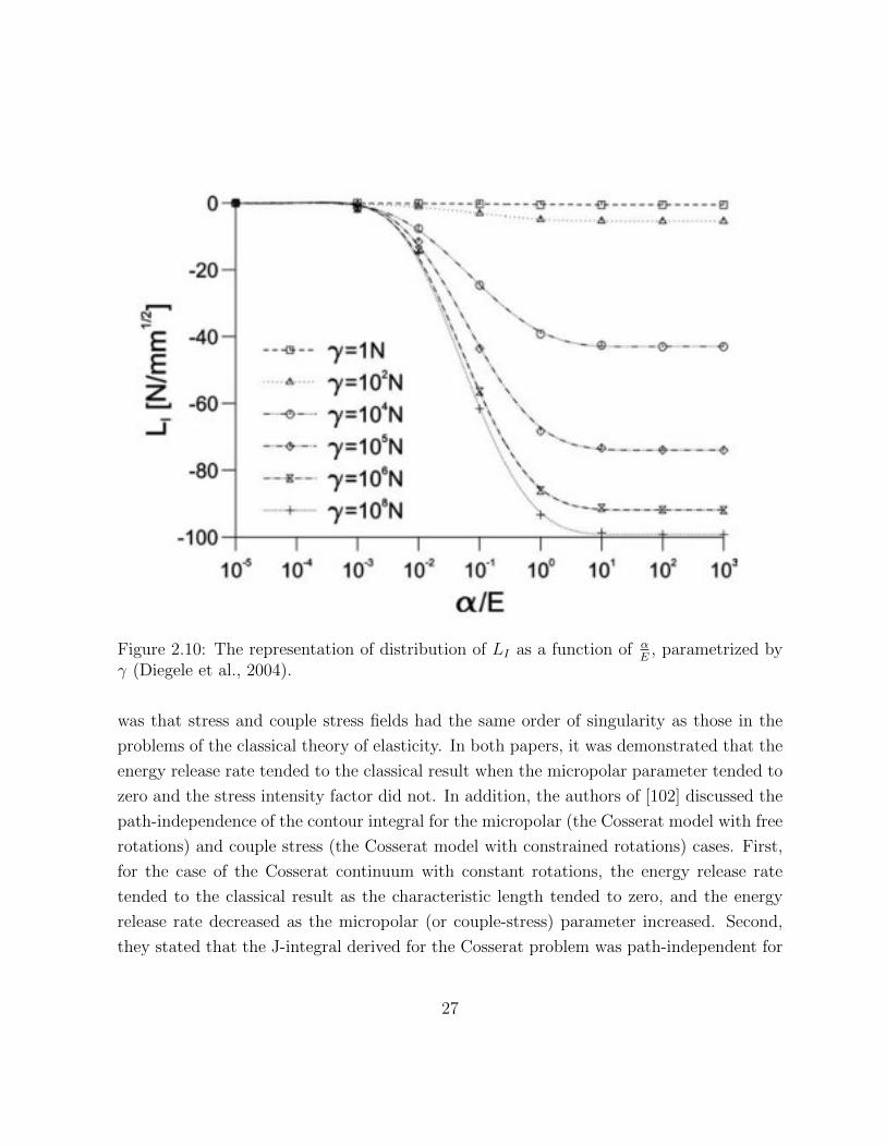
Figure 2.10: The representation of distribution of LI as a function of αE

, parametrized byγ (Diegele et al., 2004).

was that stress and couple stress fields had the same order of singularity as those in the

problems of the classical theory of elasticity. In both papers, it was demonstrated that the

energy release rate tended to the classical result when the micropolar parameter tended to

zero and the stress intensity factor did not. In addition, the authors of [102] discussed the

path-independence of the contour integral for the micropolar (the Cosserat model with free

rotations) and couple stress (the Cosserat model with constrained rotations) cases. First,

for the case of the Cosserat continuum with constant rotations, the energy release rate

tended to the classical result as the characteristic length tended to zero, and the energy

release rate decreased as the micropolar (or couple-stress) parameter increased. Second,

they stated that the J-integral derived for the Cosserat problem was path-independent for

27

both the micropolar and couple-stress problems. Another important observation was that

the energy release rate tended to the classical elastic result as γ parameter tended to zero.

The Cosserat equivalent to the J-integral has been derived in numerous ways [96, 97,

104, 105]. Following the derivation presented in [104], the energy release rate in the absence

of the body forces and body moments for plane strain micropolar elasticity is

Ji =

∫Γ

PjinjdΓ, (2.17)

where i and j are the Einstein indices, Γ is the contour about the crack tip, and n is the

normal to the contour Γ. P is the energy momentum tensor [106]:

Pij = Wδuj − σikuk,j −mi3φ3,j, (2.18)

where W is elastic energy per unit volume; σik and mi3 are the components of the stress

and couple stress tensors, respectively; uk,j = ∂uk/∂xj and φ3,j = ∂φ3/∂xj are derivatives

of the translations and rotations with respect to xj, respectively. The elastic energy is

defined as

W =1

2σijεij +

1

2mijκij, (2.19)

where εij and κij are the components of the strain and curvature tensors.

2.4 Cosserat models coupled with the Finite Element

Method

In contrast to the coupled FEM/Cosserat models, the implementation of XFEM to the

Cosserat elasticity models is not widely presented yet. Providas and Kattis in [107] in-

troduced the solution of the boundary value problem in two dimensional linear isotropic

Cosserat elasticity based on FEM. They reduced the three dimensional theory to the prob-

28

lem of the plane strain expressing it in the rectilinear coordinates. After examining three

types of elements, they showed that six-node quadratic/linear triangles produced a more

accurate result than standard three-node linear triangles and the six-node quadratic trian-

gles. Yang and Huang in [108] studied the effect of the technical constants of the micropolar

medium (i.e., micropolar Young’s modulus Em, Poisson’s ratio νm, characteristic length l,

coupling factor N , and micropolar elastic constants λ, µ, α, β, γ, κ) on the Poisson’s ratio ν

for a rectangular plate using the finite element method. They identified few dependencies

among the parameters: only the micropolar Poisson’s ratio νm could alter the Poisson’s

ratio ν of the deformed plate, and changing of any of the other three micropolar elastic con-

stants led to the change of the Poisson’s ratio. Also, either a positive or negative Poisson’s

ratio ν of the deformed plate may be obtained by changing the micropolar Poisson’s ratio

νm due to the restrictions on the elastic constants. This result is useful for understanding

the effect of the four Cosserat constants on the model.

Another important and wide implementation of the FEM/Cosserat models is found

in the field of geomechanics. The FEM/Cosserat methods can effectively model the de-

formations in layered geomaterials, where the internal length scale is associated with the

distance between the layers and their characteristics [109, 110, 111]. For these types of

problems, it is necessary to use higher-order gradient theories, such as the Cosserat theory

of elasticity, to incorporate a discontinuity in deformation at the interface of the layers and

the consequent internal length scale into the governing equations. Riahi and Curran [6]

introduced a successful implementation of the Cosserat continuum coupled with the FEM

model to simulate layered materials. In that paper, the full three-dimensional elasto-plastic

formulation of the Cosserat theory of elasticity was performed in the finite element code,

and the dependence of accuracy of the result and model parameters (such as thickness,

interaction of layers, number of layers, mesh size, boundary conditions) was studied. The

main result showed good consistency with the analytical solution predicted by the plate

theory and by the discrete element method technique. This method was capable of pre-

dicting the natural response of the layered geomaterials. The comparison of the Cosserat

model and the explicit joint finite element model was presented in [111], and the extension

of the Cosserat model to the elasto-plastic response of layered rocks was described in [112].

Another important benchmark in this field is three dimensional finite element modelling

29

of shear band localizations using the Cosserat continuum developed by Khoei et al. [5].

The history-dependent micropolar material of elasto-plasticity was examined in this paper.

The authors showed the capability of the FEM/Cosserat models to solve strain-softening

problems and compared of the classical and the Cosserat models. With a decrease of the

internal length parameter to zero, the solution converged to the classical elasticity result.

However, with the non-zero internal length parameter, the Cosserat results were more

accurate than those of the classical model.

2.5 Cosserat models coupled with the eXtended Fi-

nite Element Method

Further implementation of the Cosserat models was done by coupling them with the ex-

tended finite element method.

Khoei and Karimi [4] proposed the combined Cosserat/XFEM model to simulate the

strain localization in elasto-plastic solids. They enriched normal to the discontinuity dis-

placement and assumed the tangential displacement and micro-rotations to be continuous.

The proposed computational method was able to capture the strain localization even on

the regular basic grid. In addition, Khoei et al. [113] simulated the non-linear behaviour

of the materials (2D/3D large plasticity deformations) by representing independent of the

finite element mesh material interfaces and accomplishing the process by integrating en-

riched elements with a larger number of Gauss points whose positions were fixed in the

element.

Modelling of fracture processes in quasi-brittle materials, such as pervious concrete

and rock masses, is an important area of the research. Simulation of cracks in a solid

body is based on the continuum description. The material can be described using elasto-

plastic, damage mechanics, or coupled constitutive laws. The above mentioned materials

have discontinuous structure, which can be described as a homogenized medium using the

Cosserat elasticity theory. These models account for the elementary inter-block bending

and provide a large-scale response of a medium. This fact is important for geomechanics

problems. The characteristic length of the microstructure should be incorporated into the

30

constitutive model and leads to the necessity to use the higher-order continuum models

such as the Cosserat model. No coupled Cosserat/XFEM simulations for the cracks in the

elastic body has been done to date.

In the current research, the combined Cosserat/XFEM model is presented to perform

the fracture analysis in the Cosserat elastic solids.

31

Chapter 3

Overview of the FEM

This section describes the construction of the approximations (the weight functions and

trial solutions) for two dimensional elasticity problems.

3.1 Overview

The partial differential equations for the multi-dimensional practical problems in engineer-

ing generally have complex boundary conditions. Therefore, numerical approximation is

often the only possible way to solve these equations. The finite element method is proven

to be an effective modelling technique for a number of engineering problems.

The main approach of the finite element method is to approximate the weight functions

and trial solutions by the finite element shape functions. The important characteristic of

the FEM solution is that the quality of the solution improves with mesh refinement, or

as polynomial order of the shape functions is increased. The FEM solution converges

to the exact solution when the conditions of continuity and completeness are fulfilled.

Continuity means that the trial solutions and weight functions are sufficiently smooth.

For second order differential equations the weight functions and the trial solutions should

be C0 continuous at every point in the domain, including the interfaces of the elements.

Completeness means that the trial and weight functions and their derivatives approximate

32

the given smooth function with arbitrary accuracy, i.e are capable of assuming constant

values. For example, in the context of elasticity, the finite elements should be able to

represent rigid body motion and constant strain states exactly.

3.2 Shape functions construction

Consider an one dimensional element having two nodes, one at each end. The shape

functions for the two-node element are shown in Figure 3.1. The linear polynomial ap-

proximation has the following form [114]:

θe (x) = ae0 + ae1x. (3.1)

The approximation can be rewritten as

θe (x) = N e (x)de, (3.2)

where N e (x) = [N e1 (x) N e

2 (x)] is the element shape function matrix, and de = [θe1 θe2] is

the element nodal displacement matrix.

x

N (x)

0

1

x1 x2

N1 (x) N2 (x)

Figure 3.1: The representation of the shape functions for the two-node element.

The fundamental property of the shape functions is the interpolation property. This

33

property means that the shape functions could be used as the interpolants to fit any data.

The shape functions also obey Kronecker delta property:

N eI (xeJ) = δIJ , (3.3)

where xeJ is the coordinate of the J-node of the element and δIJ is the Kronecker delta

defined as

δIJ = 1 if I = J

0 if I 6= J. (3.4)

In two dimensional problems, the two types of the finite elements often used are triangu-

lar elements and quadrilateral elements. The three-node triangular elements or four-node

quadrilateral elements have the nodes only at their vertices. The higher order elements

have additional nodes on the edges.

The quadrilateral element is used to discretize the problem domain in the current

research. The nodes are usually numbered counterclockwise in the quadrilateral element,

starting with the left bottom node. Considering the rectangular element, the element

approximation function of the spacial coordinates (x, y) is

θe (x, y) = ae0 + ae1x+ ae2y + ae3xy, (3.5)

where the ae0, ae1, a

e2, a

e3 are the coefficient of the polynomial, chosen so that the C0 continuity

between the two elements is satisfied.

The element shape functions N e for the rectangular element are constructed by the

tensor product method. They are obtained by the product of the one dimensional shape

functions obeying the Kronecker delta property:

N e[I,J ] = N e

I (x)N eJ (y) , (3.6)

where I=1,2 and J=1,2.

34

Two dimensional shape functions for the rectangular element are

N e1 (x, y) =

1

Ae(x− xe2) (y − ye4) , (3.7)

N e2 (x, y) = − 1

Ae(x− xe1) (y − ye4) , (3.8)

N e3 (x, y) =

1

Ae(x− xe1) (y − ye1) , (3.9)

N e4 (x, y) = − 1

Ae(x− xe2) (y − ye1) , (3.10)

where Ae is the area of the element and xe and ye are the coordinates of the element nodes.

The representation of the rectangular element shape functions is shown in Figure 3.2.

1 2

34

1 2

34

1 21 2

34 3

21

4

N e1 N e2

N e3 N e4

Figure 3.2: The representation of the shape functions for the rectangular element in 2D.

FEM may employ parametric or isoparametric representation of the functions [114].

If the functions are linear along the edges of an arbitrary element and the C0 continuity

between the element is held between the two common nodes, the parametric (or direct)

construction of the shape functions may be employed, as discusses above. To construct

quadrilateral elements or the elements with the curved sides, the isoparametric shape

functions should be used. This method allows to model the structures with the complex

geometries, which is especially important for the practical engineering.

The isoparametric concept is described as the method of mapping from the parent (η, ξ)

to the physical Cartesian coordinates (x, y) (Figure 3.3). The approximation function θ

35

Node I ξI ηI1 −1 −12 1 −13 1 14 −1 1

Table 3.1: Nodal coordinates in the parametric element domain.

is presented in terms of the parent coordinates first, rather than in terms of the global

coordinates (x, y):

θe (η, ξ) = ae0 + ae1ξ + ae2η + ae3ξη. (3.11)

Figure 3.3: Mapping from the parent coordinates to the physical coordinates (Fish, Be-lytschko. A First Course in Finite Elements).

The shape functions have form of

N4QI (η, ξ) =

1

4(1 + ξIξ) (1 + ηIη) , (3.12)

where (ηI , ξI) are the nodal coordinates in the parent element, presented in Table 3.2.

The trial solution is

θe (η, ξ) = N 4Q (η, ξ)de, (3.13)

where de is the nodal displacement vector.

36

The physical coordinates are mapped by the same functions as those for the approxi-

mation. This property is an essential feature of the isoparametric element:

x (η, ξ) = N 4Q (η, ξ)xe, (3.14)

y (η, ξ) = N 4Q (η, ξ)ye, (3.15)

where xe and ye denotes the x and y coordinates of the element nodes.

The approximation constructed by quadrilateral elements is uniquely determined along

the edge of the element and is C0 continuous [114, 115].

3.3 Gauss quadrature

Gauss quadrature is the numerical integration technique for the polynomial or nearly poly-

nomial functions. The Gauss integration technique and formulas for the parent domain

(η, ξ) are presented in [114]. Following this technique, first, the physical domain (x, y)

should be mapped to the parent domain. Consider the integral over the domain Ω:

I =

∫Ωe

f (η, ξ) dΩ. (3.16)

After the integration over the ξ and η and summation over the domain Ω, the equation

(3.16) is evaluated as

I =

ngp∑i=1

ngp∑j=1

WiWj|J e (ξi, ηj) |f (ξi, ηj) , (3.17)

where ngp is number of Gauss quadrature points, Wi and Wj are the weights of the corre-

sponding quadrature points, and J e is Jacobian matrix defined as

J e = det

[∂x∂ξ

∂y∂ξ

∂x∂η

∂y∂η

]. (3.18)

37

Gauss quadrature weights and points are defined for all of the major types of the

elements and could be found in [114].

3.4 Convergence of FEM

3.4.1 Errors in the approximation

The errors of the finite element solution of a differential equation can be grouped into three

main categories [115]:

• Boundary errors due to the approximation of the domain. They occur in the two di-

mensional problems on the non rectangular domain, for which the solution is obtained

on the modified domain.

• Errors due to the numerical evaluation of the integrals and numerical computation or

round-off errors, which occur in the computation of the stiffness matrix, force vectors

and in the post-processing.

• Errors due to the approximation of the solution.

First type of errors approaches zero with the mesh refinement, because the domain is

being more accurately presented. Errors of the second type are small comparing to the

approximation errors in the most linear problems. Therefore, the approximation error is

an important quantity, which mainly defines the accuracy and the convergence properties

of the FEM/XFEM solution.

3.4.2 Measures of the errors

The evaluation of the error in the solution is generally performed with the help of norms.

The norm is the distance between two functions - the finite element approximated solution

and the exact solution. In order to calculate the difference between these two functions

the L2 and energy norms are employed.

38

The L2 norm is defined separately for translations and rotations as

‖uex − uh‖L2 =

(∫Ω

(uex − uh)2

)1/2

=

(∫Ω

((u1ex − u1h)

2 + (u2ex − u2h)2) dΩ

)1/2

,

(3.19)

‖φex − φh‖L2 =

(∫Ω

(φex − φh)2dΩ

)1/2

, (3.20)

where uex and φex are the analytical solutions, and uh and φh are the corresponding

numerical solutions.

The energy norm is defined as

‖uex − uh‖E =

(0.5

∫Ω

(εex − εh)>Du (εex − εh) dΩ + 0.5

∫Ω

(κex − κh)>Dφ (κex − κh) dΩ

)1/2

,

(3.21)

where u, ε and κ with the superscript ”ex” are the exact solutions of displacement, strain

and curvature, and with the superscript ”h” are the corresponding numerical solutions.

The L2 norm and the energy norm are normalized, respectively, as

‖uex − uh‖L2

‖uex‖L2

, (3.22)

‖uex − uh‖E‖uex‖E

. (3.23)

3.4.3 Accuracy of the solution

Error estimation shows how rapidly the approximated solution is converging to the exact

solution [114]. Consider the function to be approximated as a complete polynomial of order

p. Using the L2-norm, the error in the function could be presented as:

‖e‖L2= Chp+1. (3.24)

39

Using the energy norm, the error in the function could be presented as:

‖e‖E = Chp. (3.25)

Considering the domain without the discontinuities, for the finite element approxima-

tion with the linear element (the order of polynomial p = 1), the optimal convergence rate

is 2 in L2-norm and 1 in energy norm.

The crack in domain introduces the singularities in the stress and strain fields. This

fact leads to the reduced convergence rates of 1 in the L2-norm and 0.5 in the energy

norm in the FEM solution. On the other hand, the XFEM solution achieves the optimal

convergence rate of 2 in the L2-norm and 1 in the energy norm [116].

3.5 Verification of FEM

In order to verify the finite element code the following test may be conducted:

• Multielement displacement patch test

• Multielement force patch test

• Patch test with the known exact solution or the manufactured solution

• Convergence study

In order to fulfil the requirements of the compatibility, the multielement patch test is

introduced. The patch is a set of elements attached to a given node, which is called a patch

node. The main idea of the patch test is that the simple problem must be solved exactly

by the proper elements. The simple problem could be introduced as a displacement or

force patch test. The displacement patch test applies the boundary displacement to the

patch and verifies that the patch reproduces exactly the rigid body motion and constant

strain state. The force patch test applies the boundary forces and verifies that the patch

reproduces the exact constant stress state.

40

For more complicated problems, the patch test with the known analytical solution

or manufactured solution should be employed. In this case, the exact displacements are

applied on the boundaries of the two dimensional domain, and the finite element approx-

imation should reproduce the exact solution inside the domain. The convergence study

then shows how close the approximation is to the exact solution with the help of the error

measure, introduced above. With the mesh refinement the approximated solution must

tend to the exact solution with the optimal convergence rate for a given problem.

3.5.1 Computation scheme for the error evaluation of the XFEM

solution with the FEM exact solution

In the present research, the error evaluation of the XFEM solution was performed according

to the following steps:

1. Defining the model Define the boundary of the physical model, the boundary and

loading condition, the material model.

2. Front tracking Define the crack geometry (front) using level set method.

3. FEM solver Obtain the FEM solution of the problem for a very fine mesh.

4. Saving FEM results Save the reference results of the FEM computation: nodes in-

formation, connectivity matrix, assigned degrees of freedom, displacement vector.

5. XFEM solver Define mesh sizes sequence.

6. Obtain the XFEM solution of the problem for a given mesh.

7. Post-processing Load the FEM solution results. Load the XFEM solution results.

8. For n = 1 to number of elements, define the element quadrature order depending on

the element enrichment type (Heaviside enrichment, branch functions enrichment, no

enrichment).

41

9. For q = 1 to number of quadrature points in the element, obtain the global coordinates

of the quadrature point.

XFEM FEM

Obtain the vector of element nodal Define the element in the FEM mesh containing

displacements from the XFEM the point, using the global coordinates

solution (step 6). of the quadrature point.

Calculate the strain and the curvature Obtain the vector of element nodal displacements

at the point - approximated values. from the FEM solution (step 3).

Calculate the strain and the curvature - exact values.

Calculate the relative error in the energy using the equation (3.21).

10. Got to the step 9.

11. Go to the step 8.

12. Go to the next mesh for the XFEM solver (step 6).

42

Chapter 4

XFEM Model of the Crack in the

Cosserat Elastic Material

In this section, the governing equations are presented, the strong and the weak forms for

a crack in a Cosserat medium are developed, the discrete equations are derived, the crack

opening model in a Cosserat medium is described, and the J-integral computational scheme

is presented.

4.1 Governing equations

Consider the two dimensional domain Ω bounded by Γ, as shown in Figure 4.1. Boundary

Γ consists of the sets Γu, Γφ, Γt, and Γm, where displacements u, microrotations φ, surface

forces (traction) t, and surface couple forces (moment) M are prescribed, respectively. The

internal surface of crack is denoted by Γcr. Boundary properties are as follows:

Γu ∩ Γt = ∅ and Γu ∪ Γt = Γ, (4.1)

Γφ ∩ ΓM = ∅ and Γφ ∪ ΓM = Γ. (4.2)

The case of plane strain is considered. The components of displacement and rotations

43

Γu

Γφ

ΓtΓM

Γcr

φu

M

t

Ω

Γ

Figure 4.1: Body with external and internal boundaries subjected to loads.

are u ≡ (u1, u2, 0) and φ ≡ (0, 0, φ3), respectively.

In two dimensions, governing equilibrium equations are

∇ · σ + bσ = 0, (4.3)

∇ ·m + bm + σ = 0, (4.4)

where σ is the Cauchy stress, bσ is the external forces, m is the couple force stress, bm is

the external moment, and σ = σ21 − σ12.

The Neumann boundary conditions are

σ · n = t on Γt, (4.5)

m · n = M on ΓM , (4.6)

where n is the unit outward normal to Γ.

The Dirichlet boundary conditions are

u = u on Γu, (4.7)

φ = φ on Γϕ. (4.8)

44

The boundary conditions on the crack surface are

σ · ncr = 0 and m · ncr = 0 on Γcr, (4.9)

where ncr is the normal to the crack surface Γcr.

The translations, u, and the microrotations, φ, are taken to be the independent vari-

ables. The strain, ε, and the curvature, κ, vectors have the following relationships with

these variables:

ε = ∇u− φ, (4.10)

κ = ∇φ, (4.11)

where φ =

[0 −φ3

φ3 0

].

The linear constitutive equations for the coupled model are

σ = Du : ε, (4.12)

m = Dφ : κ, (4.13)

whereDu andDφ are the elastic moduli tensors which for an isotropic material are defined

as

Du =

2µ+ λ λ 0 0

λ 2µ+ λ 0 0

0 0 µ− α µ+ α

0 0 µ+ α µ− α

(4.14)

and

Dφ =

[γ + κ 0

0 γ + κ

], (4.15)

where µ, λ, α, γ and κ are material constants.

45

4.2 Weak form

The spaces of admissible displacement fields are

U =u ∈ H1,u = u on Γu,u is discontinuous on Γcr

, (4.16)

Φ =φ ∈ H1, φ = φ on Γφ, φ is discontinuous on Γcr

. (4.17)

The test functions spaces are

U0 =w ∈ H1,w = 0 on Γu

, (4.18)

Φ0 =v ∈ H1, v = 0 on Γφ

. (4.19)

The weak forms of the equilibrium equations are constructed by multiplying the govern-

ing equations (4.3) and (4.4) by an arbitrary functions w ∈ U0 and v ∈ Φ0, respectively,

and integrating over the domain Ω. After integrating by parts and substituting the consti-

tutive model for the stresses (4.12) and (4.13), we have the weak form of coupled boundary

value problem of Cosserat elasticity: Find u ∈ U and φ ∈ Φ such that∫Ω

∇w : σdΩ =

∫Ω

w · bσdΩ +

∫Γt

w · tdΓ, ∀w ∈ U0, (4.20)∫Ω

∇v ·mdΩ =

∫Ω

v bmdΩ +

∫ΓM

v MdΓ, ∀v ∈ Φ0. (4.21)

It was shown in [57] that the weak form is equivalent to the strong form.

4.3 Discrete equations

In the following subsection we will develop the discrete equations for a domain with a single

crack. The extension to the case of multiple cracks follows in a straightforward manner.

Consider a crack Γcr passing through a discretized domain, as shown in Figure 4.2.

46

y

x

y

x

Γcr

Figure 4.2: Illustration of a two dimensional domain containing a crack Γcr. The circlednodes are enriched by the Heaviside function, and the squared nodes are enriched by thecrack tip enrichment function.

The level set method is employed to represent the crack position in the domain and

track the propagation of the crack. The level set allows to describe the complicated crack

geometry by a functional representation. According to the [75], the crack is considered

as a one-dimensional curve in the two-dimensional space. The signed distance function is

defined as

f (x) = ± min ‖x− xΓcr‖, (4.22)

where x is a point in the domain, xΓcr is the point on the crack surface, and the sign is

different on the two sides of the crack surface.

The crack surface Γcr is represented as the zero level set of a function f (x). The crack

tip position is represented by the zero level set of a function g (x), which intersects the

crack tip and is orthogonal to the zero level set of a function f (x). The signs of the

distance for the f (x) and g (x) functions are shown in Figure 4.3. The crack is defined at

47

Γcr

xtip

f(x) = 0

g(x) = 0

f(x) > 0

f(x) < 0

g(x) > 0

g(x) < 0

Figure 4.3: Level set method for the crack growth modelling.

the locations where the following conditions are true:

f (x) = 0, (4.23)

g (x) ≤ 0. (4.24)

This method allows to assign discrete values of level set functions at each node of the

elements. Thus, the level set functions fh (x) and gh (x) are the approximations of the

signed distance functions f (x) and g (x):

fh (x) =∑I

NI (x)f I , (4.25)

gh (x) =∑I

NI (x) gI , (4.26)

where N (x) are the standard bilinear finite element shape function.

The level set function representing the initial crack is constructed by computing the

signed-distance function for the crack. The initial crack is then extended tangentially from

its tip, and the signed-distance function is constructed from this extended crack. Crack

growth is modelled by appropriately updating the f (x) and g (x) functions.

48

Following a procedure similar to the original XFEM [69]:

uh(x) =∑I∈S

NI(x)duI +∑J∈Scr

NJ(x)[H(f(x))−H(f(xJ))]auJ+

+∑

K∈Stip

NK(x)M∑m=1

[Fm(r, θ)− Fm(rn, θn)]bumK , ∀x ∈ Ω, (4.27)

φh(x) =∑I∈S

NφI (x)dφI +

∑J∈Scr

NφJ (x)[H(f(x))−H(f(xJ))]aφJ+

+∑

K∈Stip

NφK(x)[F φ(r, θ)− F φ(rn, θn)]bφK , ∀x ∈ Ω, (4.28)

where S is the set of all nodes, Scr is the set of nodes with support crossed by the crack

faces, Stip is the set of nodes inside the predefined area around the crack tip, NI are

the standard finite element shape functions for the vector field (translations), NφI are the

standard finite element shape functions for the scalar field (microrotations), f(x) is signed

distance to Γcr, duI and dφI are the standard FEM nodal translational and rotational degrees

of freedom, auJ and aφJ are the Heaviside function enriched degrees of freedom, and buK and

bφK are the branch function enriched degrees of freedom. Scr and Stip are the sets of circled

and squared nodes,respectively (Figure 4.2):

Stip =K|f 2(xK) + g2(xK) 6 r2

tip

, (4.29)

Scr = J |min(f(xJ)) ·max(f(xJ)) 6 0 and max(g(xJ)) > 0, J /∈ Stip , (4.30)

where rtip is predefined radius of a domain around the crack tip to be enriched with a

special tip enrichment functions.

Careful analysis of the asymptotic crack tip solution for a Cosserat material [98] reveals

that these solutions are spanned by the same functions as those from William’s series

expansion. Therefore, as in the standard XFEM, it is convenient to enrich the translation

49

field in the crack tip domain using the branch functions:

Fm = √r sin

θ

2,√r cos

θ

2,√r sin

θ

2sin θ,

√r cos

θ

2sin θ, (4.31)

where (r, θ) are the local polar coordinates with origin at the crack tip.

A similar analysis shows that the crack tip field for the microrotations is spanned by

the function:

F φm =

√r sin

θ

2. (4.32)

The Heaviside step function (discontinuous function) is defined in local coordinate

system and given by

H(z) =

1 if z > 0

0 otherwise. (4.33)

The jump in displacement (both translation and microrotation) across the crack Γcr is

[|u|] = u+(x)− u−(x), x ∈ Γcr, (4.34)

[|φ|] = φ+(x)− φ−(x), x ∈ Γcr, (4.35)

where u+ and u− (φ+ and φ−) are the translations (rotations) above and below the crack,

respectively.

Substituting the displacement approximation (4.27) and (4.28) into the (4.34) and

(4.35) and simplifying, we have

[|u|] =∑J∈Scr

NJauJ on Γcr, (4.36)

[|φ|] =∑J∈Scr

NJaφJ on Γcr. (4.37)

These equations mean that solution is discontinuous across the crack; auJ shows the

50

opening of the crack.

Following Galerkin approach, the test functions w and v are taken in the same form as

for the translations (4.27) and rotations (4.28), respectively:

wh(x) =∑I∈S

NI(x)δwI +∑J∈Scr

NJ(x)[H(f(x))−H(f(xJ))]δauJ+

+∑

K∈Stip

NK(x)M∑m=1

[Fm(r, θ)− Fm(rn, θn)]δbumK , ∀x ∈ Ω, (4.38)

vh(x) =∑I∈S

NφI (x)δvI +

∑J∈Scr

NφJ (x)[H(f(x))−H(f(xJ))]δaφJ+

+∑

K∈Stip

NφK(x)[F φ(r, θ)− F φ(rn, θn)]δbφK , ∀x ∈ Ω. (4.39)

Substituting the approximations for the displacements (4.27), (4.28) and the test func-

tions (4.38), (4.39) into the weak forms of the equilibrium equations (4.20) and (4.21) the

following discrete equation are obtained:

K11 K12 K13 K14 K15 K16

K21 K22 K23 K24 K25 K26

K31 K32 K33 K34 K35 K36

K41 K42 K43 K44 K45 K46

K51 K52 K53 K54 K55 K56

K61 K62 K63 K64 K65 K66

du

dφ

au

aφ

bu

bφ

=

fext1

fext2

fext3

fext4

fext5

fext6

(4.40)

where du and dφ are the standard displacement nodal degrees of freedom that correspond

to the translation and rotation, respectively, au and aφ are the vectors of additional degrees

of freedom due to Heaviside enrichment term in the approximations, and bu and bφ are the

vectors of the additional degrees of freedom due to the crack tip enrichment. Sub-matrices

K11, ...,K66 and fext1 , ..., fext6 are defined in the Appendix A.

Remark 1. K is not symmetric, unlike in FEM/XFEM classical elasticity.

51

Remark 2. The length of vectors au, aφ,bu and bφ are very small compared to vectors

du and dφ, so XFEM does not significantly increase the cost of solving (4.40).

4.4 Numerical integration

Several aspects that are crucial in order to obtain accurate results and optimal convergence

rates are listed below [117]:

• Numerical integration is an important issue in the XFEM. The proper integration

rules in the elements cut by a crack and containing a crack tip should be considered.

• The fixed enrichment area around a crack tip (geometrical enrichment) is crucial to

obtain optimal convergence rates. It allows to get twice better energy convergence

rate than in case of the topological enrichment, when only particular number of nodes

layers are enriched.

• Blending elements allows for the smooth transition between enriched and unenriched

subdomains by using the special weight function with compact support.

The considerable amount of works on the research of numerical integration for the

XFEM is presented in [118]. There are two difficulties for the integration in the XFEM.

First, in elements cut by the interface, the shape functions may be discontinuous. Second,

if the element contains a crack tip, the enriching functions and their gradients are singular.

That means that the integration scheme depends on whether the element is enriched and on

the type of enrichment. The integration of unenriched elements is done in the standard way

using Gauss quadrature of the required order. If the element is fully cut by the interface,

i.e. enriched by the Heaviside step function, the sub-integration is employed. The element

is divided into triangles in such a way that the crack surface is aligned with the edges

of two triangles [69]. In the present research, for both unenriched elements and elements

enriched with the Heaviside function the Gauss quadrature of order 2 is employed. The

subintegration is used in the latter case.

52

If the element contains the crack tip, the element is divided into the several sub-triangles

having one vertex at the crack tip [119]. In each triangle the higher order Gauss quadrature

is used. This creates the concentration of integration points near the node of the triangle

located at the crack tip. This technique with the Gauss quadrature of order 15 is employed

in the present research (Figure 4.4).

−1 −0.8 −0.6 −0.4 −0.2 0 0.2 0.4 0.6 0.8 1−1

−0.8

−0.6

−0.4

−0.2

0

0.2

0.4

0.6

0.8

1

Figure 4.4: The representation of the Gauss quadrature rule in the element containingcrack tip.

Considering the branch function zone enrichment, there are two ways to define the

branch functions enrichment zone around the crack tip: the geometrical enrichment and

the topological enrichment. First approach defines the enriched nodes within the constant

radius. The second approach defines the enriched nodes in the particular number of nodes

layers around the crack tip. To get optimal behaviour in energy norm for the XFEM, the

geometrical enrichment should be considered. In the case of the geometrical enrichment,

the branch function enrichment area is independent of the mesh size. Two types of crack

tip zone enrichment are illustrated in Figure 4.5-4.6.

Another important issue in the XFEM is the blending elements. The blending elements

are those that have some of the nodes enriched and some of them unenriched [116]. The

standard enrichment can add parasitic terms to the approximation space of the blending

elements, i.e. the reproducing property of the partition of unity is lost. No difficulties

occurs in the blending of the shifted Heaviside enrichment, because the enrichment is

53

only considered for the elements cut by crack. However, for the tip enrichment zone, the

blending might play an important role to reduce the error value.

Concluding, the use of proper integration rules, depending on the type of elements is

crucial for the accuracy of the solution and obtaining optimal convergence rates. The dif-

ferences in convergence rates of the finite element method, extended finite element method

with topological and geometrical tip enrichments, and without tip enrichment are shown

further in Chapter ”Numerical Examples”.

0 10 20 30 40 50 60 70 80 90 1000

10

20

30

40

50

60

70

80

90

100

(a)

0 10 20 30 40 50 60 70 80 90 1000

10

20

30

40

50

60

70

80

90

100

(b)

Figure 4.5: Selected elements for the geometrical enrichment with the number of elements:(a) 11×11, (b) 51×51.

54

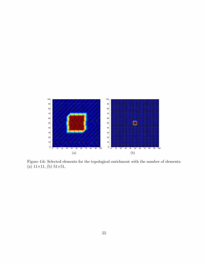
0 10 20 30 40 50 60 70 80 90 1000

10

20

30

40

50

60

70

80

90

100

(a)

0 10 20 30 40 50 60 70 80 90 1000

10

20

30

40

50

60

70

80

90

100

(b)

Figure 4.6: Selected elements for the topological enrichment with the number of elements:(a) 11×11, (b) 51×51.

55

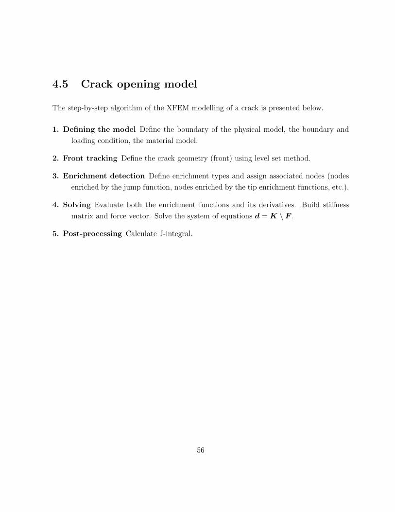
4.5 Crack opening model

The step-by-step algorithm of the XFEM modelling of a crack is presented below.

1. Defining the model Define the boundary of the physical model, the boundary and

loading condition, the material model.

2. Front tracking Define the crack geometry (front) using level set method.

3. Enrichment detection Define enrichment types and assign associated nodes (nodes

enriched by the jump function, nodes enriched by the tip enrichment functions, etc.).

4. Solving Evaluate both the enrichment functions and its derivatives. Build stiffness

matrix and force vector. Solve the system of equations d = K \ F .

5. Post-processing Calculate J-integral.

56

4.6 Computation scheme of the J-integral evaluation

1. Load FEM/XFEM solution and the crack information to the Postprocessor.

2. Define the contour radius and location, number of sectors.

3. For n = 1 to number of sector, calculate Jacobian and define the Gauss quadrature

order.

4. For q = 1 to number of quadrature points, obtain the global coordinates of the quadra-

ture point, define the element of the mesh containing the point, obtain the vector

of element nodal displacements from the displacement vector, define a normal to a

contour at a point; calculate stress, strain, curvature components, derivatives of the

displacements, and strain energy at the point; calculate J-integral at a point and sum

the value to the global J-integral.

5. Go to step 4.

6. Go to step 3.

57

Chapter 5

Numerical Examples

In this chapter, the numerical examples of cracks under the assumption of the plane strain

in two-dimensional Cosserat elastic medium are presented. The series of patch tests and

convergence studies in the first three examples verify the method and demonstrate the

convergence properties of the FEM and the XFEM solutions of the edge crack problem

in a Cosserat elastic medium. The convergence properties of the XFEM solution of the

edge crack problem under tension and shear loading are demonstrated. The forth example

presents the verification of the contour J-integral calculation. In the fifth example a com-

parison of the J-integral for the Cosserat elasticity and the classical elasticity is presented

and discussed.

5.1 Introduction

As stated in [98], the Cosserat parameter α varies from 0 (classical linear elasticity) to ∞(couple stress linear elasticity) and has a huge impact on the asymmetrical properties of

the stress and strain tensors. Several problems with α 6= 0 were solved to demonstrate the

effectiveness of the developed XFEM/Cosserat method.

In order to perform convergence studies in the following examples, the normalized

energy norms are employed, see Section 3.4.2 for details. For the following examples, the

58

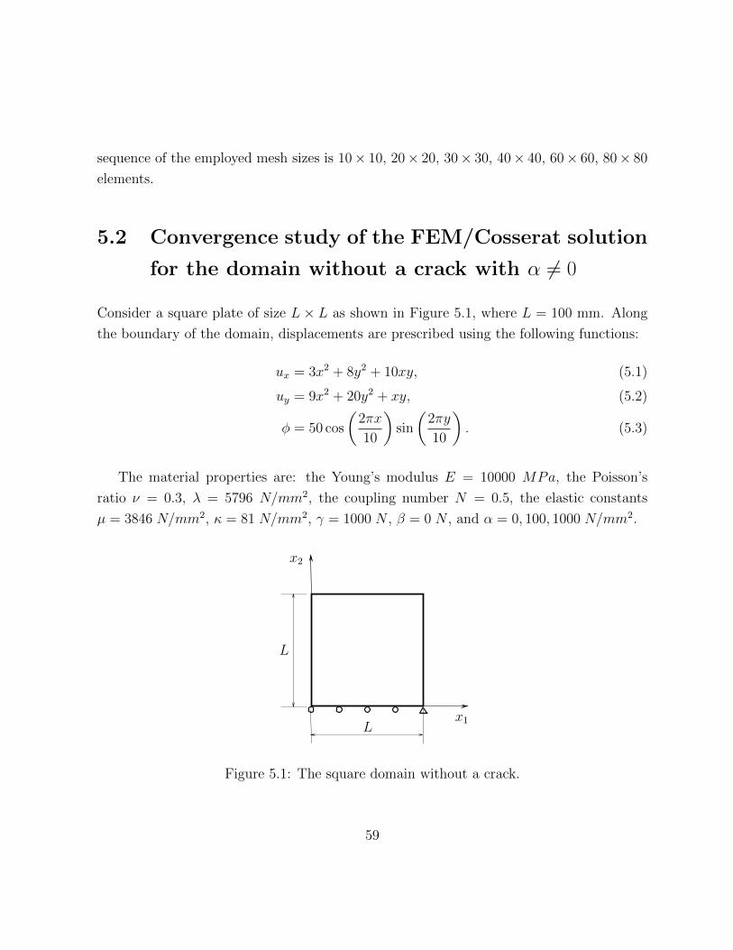
sequence of the employed mesh sizes is 10× 10, 20× 20, 30× 30, 40× 40, 60× 60, 80× 80

elements.

5.2 Convergence study of the FEM/Cosserat solution

for the domain without a crack with α 6= 0

Consider a square plate of size L × L as shown in Figure 5.1, where L = 100 mm. Along

the boundary of the domain, displacements are prescribed using the following functions:

ux = 3x2 + 8y2 + 10xy, (5.1)

uy = 9x2 + 20y2 + xy, (5.2)

φ = 50 cos

(2πx

10

)sin

(2πy

10

). (5.3)

The material properties are: the Young’s modulus E = 10000 MPa, the Poisson’s

ratio ν = 0.3, λ = 5796 N/mm2, the coupling number N = 0.5, the elastic constants

µ = 3846 N/mm2, κ = 81 N/mm2, γ = 1000 N , β = 0 N , and α = 0, 100, 1000 N/mm2.

x2

L

L

x1

Figure 5.1: The square domain without a crack.

59

As shown in Figure 5.2, the obtained convergence rates for various α are in order of

≈ 1 in the energy norm, which is the optimal convergence rates for the domain without a

crack. This example shows that the FEM solution of the Cosserat problem with α 6= 0 is

correct and could be used as the exact solution for the following convergence test of the

XFEM problem.

100

101

10−3

10−2

10−1

element size

rela

tive

erro

r

Energy norm

FEM alpha=0 (slope 1.000)FEM alpha=100 (slope 0.995)FEM alpha=1000 (slope 0.989)

Figure 5.2: Convergence rates of the FEM solutions for the α=0, 100, 1000.

60

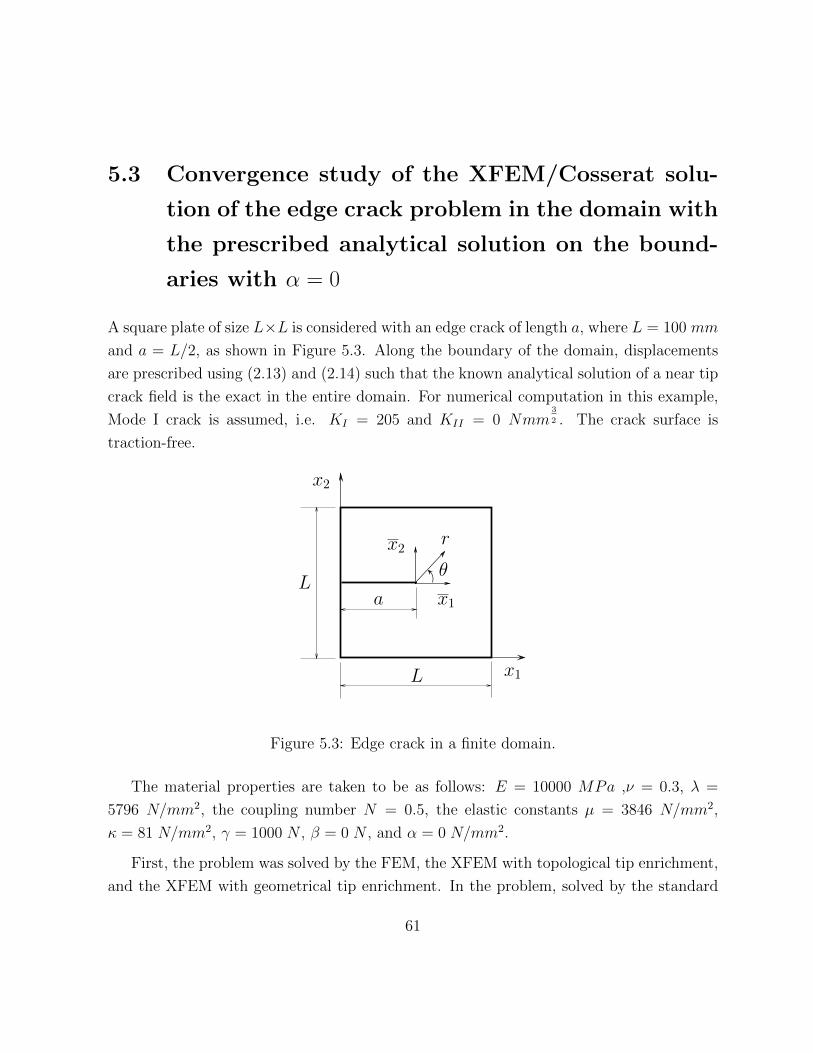
5.3 Convergence study of the XFEM/Cosserat solu-

tion of the edge crack problem in the domain with

the prescribed analytical solution on the bound-

aries with α = 0

A square plate of size L×L is considered with an edge crack of length a, where L = 100 mm

and a = L/2, as shown in Figure 5.3. Along the boundary of the domain, displacements

are prescribed using (2.13) and (2.14) such that the known analytical solution of a near tip

crack field is the exact in the entire domain. For numerical computation in this example,

Mode I crack is assumed, i.e. KI = 205 and KII = 0 Nmm3

2 . The crack surface is

traction-free.

x1

x2

x1

x2θ

r

a

L

L

Figure 5.3: Edge crack in a finite domain.

The material properties are taken to be as follows: E = 10000 MPa ,ν = 0.3, λ =

5796 N/mm2, the coupling number N = 0.5, the elastic constants µ = 3846 N/mm2,

κ = 81 N/mm2, γ = 1000 N , β = 0 N , and α = 0 N/mm2.

First, the problem was solved by the FEM, the XFEM with topological tip enrichment,

and the XFEM with geometrical tip enrichment. In the problem, solved by the standard

61

FEM, the crack surface is aligned with the element edges, and the crack tip is located at

the node. In the XFEM computation discontinuity is presented independently of the mesh.

The results of the convergence study of the Mode I edge crack in the square domain are

presented in Figure 5.4. The sub-optimal convergence rates of ≈0.5 in energy norm are

obtained. The convergence rates of the FEM solution are reduced due to the presence of

singularity in the vicinity of the crack tip. The problem solved by the XFEM technique

with the geometrical tip enrichment shows optimal convergence rates of ≈1 in energy

norm. The convergence of the XFEM solution with the topological tip enrichment is

studied, as well. The suboptimal convergence rate of ≈0.5 in energy norm is obtained by

that method, as expected. The crucial issues for obtaining the optimal convergence rates

are the use of special integration methods in the crack-tip element and the element cut

by crack, branch function enrichment of the fixed area around the crack tip (so called,

geometrical enrichment) and the specific treatment of the blending elements. All of the

above mentioned techniques are described in detail in Section 4.4 ”Numerical integration”.

Analogous convergence study was performed for the Mode II edge crack problem, i.e.

KI = 0 and KII = 200 Nmm3

2 . Similarly to the presented results of the Mode I edge

crack, the optimal convergence rates are obtained by the XFEM with the geometrical tip

enrichment.

62

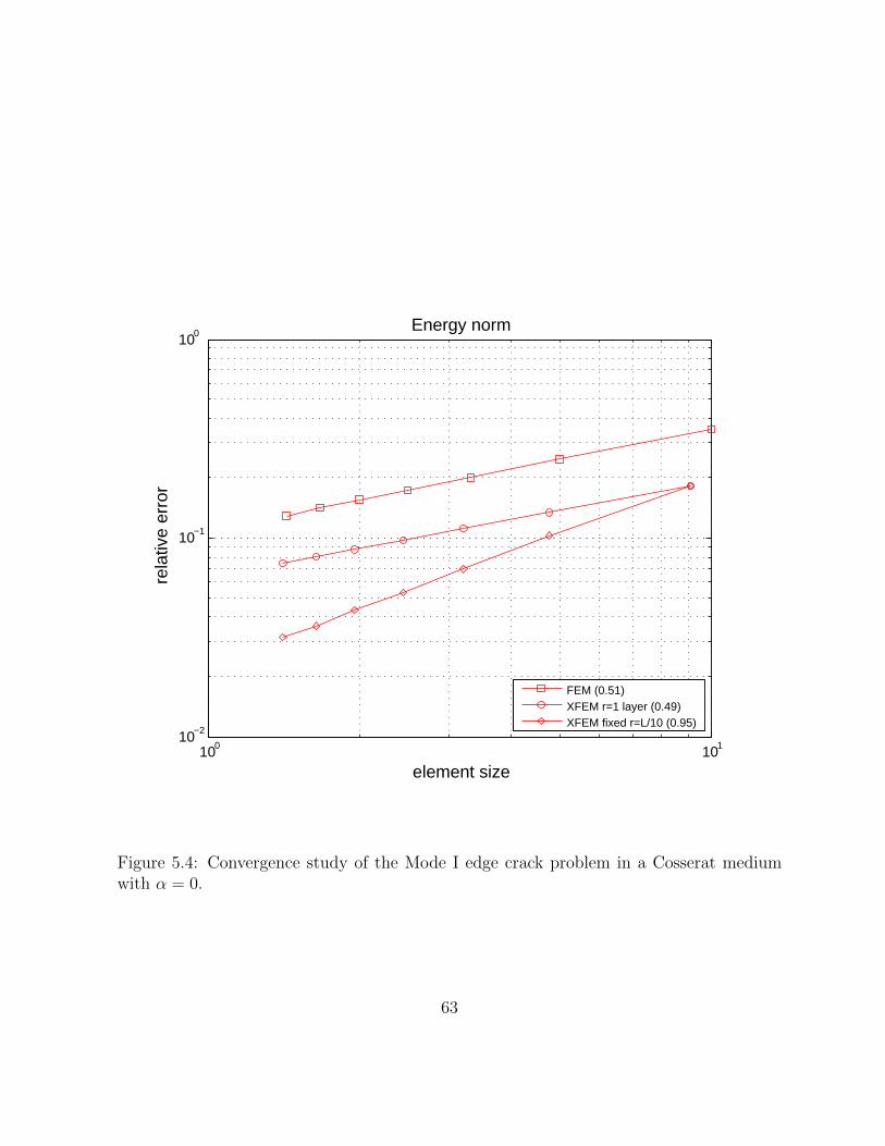
100 10110−2

10−1

100

element size

rela

tive

erro

r

Energy norm

FEM (0.51)XFEM r=1 layer (0.49)XFEM fixed r=L/10 (0.95)

Figure 5.4: Convergence study of the Mode I edge crack problem in a Cosserat mediumwith α = 0.

63

Second, the tip enrichment types were studied to find the optimal way to asymptotically

enrich the nodes in the vicinity of the crack tip. Considering the topological tip enrichment,

Figure 5.5 shows the dependence of the error values on the number of the enriched with

the branch functions nodes layers around the crack tip. With the increasing number of

enriched nodes layers, the error value is getting smaller. This is explained by the fact that

larger area is enriched with the known asymptotic solution.

Considering the geometrical tip enrichment, the studies of the convergence rates de-

pending on the asymptotic enrichment radius are presented in the Figure 5.6. Although,

the error value is getting smaller for the bigger tip radius enrichment, this causes the dra-

matically increased computational time. With the increased radius of tip enrichment, the

number of enriched nodes and elements with higher order Gauss quadrature are getting

larger. On the other hand, the radius of tip enrichment zone equal or smaller than L/15

causes the less accurate solution. Taking into account all of these observations, the optimal

enrichment radius of L/10 is adopted for the further modelling.

64

100.2 100.3 100.4 100.5

10−1

element size

rela

tive

erro

r

Energy norm

XFEM r=1 layer (0.493)XFEM r=2 layers (0.485)XFEM r=3 layers (0.47)XFEM r=4 layers (0.461)

Figure 5.5: Convergence study for the coupled Mode I edge crack case solved by XFEMwith topological tip enrichment with varying number of enriched nodes layers from 1 to 4.

65

100.2 100.3 100.4 100.510−2

10−1

element size

rela

tive

erro

r

Energy norm

XFEM r=L/5 (1.02)XFEM r=L/10 (0.995)XFEM r=L/15 (0.983)XFEM r=L/20 (1.173)

Figure 5.6: Convergence study for the coupled Mode I edge crack case solved by XFEMwith geometrical tip enrichment with varying radius from L/5 to L/20.

66

5.4 Convergence study of the XFEM/Cosserat solu-

tion of the edge crack problem with α 6= 0

5.4.1 Mode I edge crack

A square plate of size L × L is considered with an edge crack of length a as shown in

Figure 5.7, where L = 100 mm and a = L/2. The domain is fixed at the bottom, and the

displacement u2 = 5 mm in x2 direction is prescribed along the top edge. The microro-

tations φ = 0 are prescribed along the bottom and top edges of the domain, which allows

for the microrotations to emerge around the crack tip. The crack surface is traction-free.

The plain strain condition is assumed. The material properties are: the Young’s modulus

E = 10000 MPa, the Poisson’s ratio ν = 0.3, λ = 5796 N/mm2, the elastic constants

µ = 3846 N/mm2, κ = 81 N/mm2, γ = 1000 N , β = 0 N . As it was mentioned above,

α = 0 reduces the problem to the one of the classical elasticity, and α → ∞ implies the

couple stress elasticity problem. For this example, α was taken to be 103 N/mm2.

x2

x1

x2θ

r

a

L

L

u2

x1

Figure 5.7: The domain with an edge crack under tension.

In order to perform the convergence study for the Mode I and II edge crack problems,

the normalized energy norm is employed as a convergence criterion. The employed mesh

67

sizes are 11 × 11, 21 × 21, 31 × 31, 41 × 41, 51 × 51,71 × 71 elements. The solution of

the addressed Mode I edge crack problem by the Finite Element Method with the mesh of

40,000 elements was taken to be the exact solution. Two types of the tip enrichment zones

were considered for the convergence study of the XFEM: the topological tip enrichment

of the one layer of nodes around the crack tip, the geometrical tip enrichment of the size

L/10. Figure 5.8 shows three convergence curves and the corresponding convergence rates

for the Mode I edge crack solution in a Cosserat medium.

As expected, the optimal convergence rate of ≈1 in the energy norm for the XFEM

with geometrical enrichment is obtained. The suboptimal convergence rates of ≈0.5 in

energy norm are obtained for the XFEM solutions with topological tip enrichment and for

the FEM solution.

68

100

101

10−2

10−1

element size

rela

tive

erro

r

FEM (0.58)XFEM r=1 layer (0.528)XFEM r=L/10 (0.953)

Figure 5.8: Convergence rates of the XFEM solutions of the edge crack problem under thetension loading with α=1000.

69

5.4.2 Mode II edge crack

In the second example, Mode II edge crack problem is studied. Consider a square plate

of size L × L with an edge crack of length a, as shown in Figure 5.9. The length of

the plate is L = 100 mm, and the crack size is a = L/2. The domain is fixed at the

bottom. The displacement u1 = 5 mm in x1 direction is prescribed along the top edge.

The microrotations are prescribed to be φ = 0 along the bottom and top edges of the

domain. The crack surface is traction-free. The plain strain condition is assumed. The

material properties are: the Young’s modulus E = 10000 MPa, the Poisson’s ratio ν = 0.3,

λ = 5796 N/mm2, the elastic constants µ = 3846 N/mm2, κ = 81 N/mm2, γ = 1000 N ,

β = 0 N .

x2

x1

x2θ

r

a

L

L

u1

x1

Figure 5.9: The square domain with an edge crack under shear loading.

The convergence rates are shown in Figure 5.10. For the Mode II edge crack problem in

a Cosserat medium, the optimal convergence rate of ≈ 1 in energy norm was obtained for

the XFEM solution with the geometrical tip enrichment, and the suboptimal convergence

rate of ≈ 0.5 in energy norm was obtained for the XFEM solution with the topological tip

enrichment.

For both Mode I and II edge crack problems, the slight decrease in the convergence

rates from the optimal values is observed, but expected. In order to get higher convergence

70

100 10110−2

10−1

element size

rela

tive

erro

rEnergy norm

FEM (0.5)XFEM r=1 layer (0.52)XFEM r=L/10 (0.916)

Figure 5.10: Convergence rates of the FEM solutions of the edge crack problem under theshear loading for the α=1000.

rates, the very fine mesh should be considered for the exact FEM solution. Although, the

computational time will increase drastically.

Concluding, the results of the convergence studies for the cracks of Modes I and II in

the Cosserat medium allows us to rely on the developed XFEM model with confidence.

71

5.5 Calculation of the J-integral in a Cosserat medium

5.5.1 Verification of the J-integral calculation

Consider a square plate of size L × L, with an edge crack of length a, L = 100 mm and

a = L/2, as shown in Figure 5.11. The known asymptotic displacement field solutions

(2.13-2.14) are prescribed on the boundaries of the domain. The crack surface is traction-

free. The material properties are: the Young’s modulus E = 10000 MPa, the Poisson’s

ratio ν = 0.3, λ = 5796 N/mm2, the coupling number N = 0.5, the elastic constants

µ = 3846 N/mm2, κ = 81 N/mm2, γ = 1000 N , β = 0 N , and α = 0 N/mm2.

x1

x2

x1

x2θ

r

a

L

L

Figure 5.11: The domain with an edge crack. The asymptotic field solutions are prescribedon the boundaries.

First, the path-independence of the J-integral is studied. The path-independence is

the important characteristic of the contour integral. In this research, the contour of the

J-integral is assumed to be a circle with its center coinciding with the crack tip. Figure 5.12

shows that the calculated J-integral is converging and path-independent. The case with

geometrical tip enrichment of radius L/10 gives more accurate values and smooth behaviour

of the J-integral curve. The kink at the R = 10mm corresponds to the end of the tip

enrichment radius 10. As well, the slight disinclination of the J-integral values is observed

72

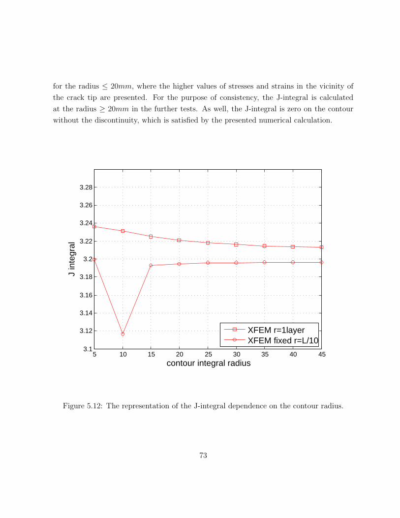
for the radius ≤ 20mm, where the higher values of stresses and strains in the vicinity of

the crack tip are presented. For the purpose of consistency, the J-integral is calculated

at the radius ≥ 20mm in the further tests. As well, the J-integral is zero on the contour

without the discontinuity, which is satisfied by the presented numerical calculation.

5 10 15 20 25 30 35 40 453.1

3.12

3.14

3.16

3.18

3.2

3.22

3.24

3.26

3.28

contour integral radius

J in

tegr

al

XFEM r=1layerXFEM fixed r=L/10

Figure 5.12: The representation of the J-integral dependence on the contour radius.

73

Second test compares the numerically calculated for the reduced to the classical case

J-integral with the one obtained analytically. In the classical theory of elasticity, J-integral

for the Mode I crack is calculated in the following way:

J =KI

2

E∗, (5.4)

where E∗ = E1−ν2 for the plane strain case and E∗ = E for the plane stress case. Only the

Cosserat model, reduced to the classical, could be tested this way, as there is no known

relationship between LI and J. The numerical values of the J-integral was found to be less

than 1% different from the analytically obtained values.

In addition, the J-integral can be approximated as the change in the energy of the do-

main due to crack length increment, i.e4U/4a. Considering a mesh of 101×101 elements

with the crack increment 4a = 3mm, for the Mode I crack case the deviation from the

analytical value was of 4%, and for the Mode II crack case the deviation was of 5%. Taking

into account the fact that this approximation is valid for the crack increment approaching

zero 4a → 0, the obtained results are accurate enough to consider the calculation of the

J-integral in the Cosserat elastic medium to be correct.

Forth, the dependence of the J-integral from KI is studied and shown in Figure 5.13.

The slope of the line is 2, and the y-intercept is 7.58×10−5, which corresponds to the value

of KI2 (1− ν2), as expected from the power law (5.4) for the case of plane strain.

The obtained results verify the most important characteristics of the contour J-integral,

which allow us to proceed to the study of the energy release rate for the Cosserat medium.

74

100 101 102 10310−5

10−4

10−3

10−2

10−1

100

101

KI

J in

tegr

al

XFEM r=1layerXFEM fixed r=L/10

Figure 5.13: The representation of dependence of J-integral from KI with LI = 0.

75

5.5.2 Comparison of the J-integral for the Cosserat elastic medium

and classical elastic medium

Consider the domain illustrated in Figure 5.14. A plate of height L and width W contains

an edge crack of length a, where L/W = 2, W = 100 mm and a has varying value. The

bottom edge of the domain is fixed. The stress σ = 3 MPa is applied at the top edge

of the domain. The Young’s modulus is E = 10000 MPa, the Poisson’s ratio is ν = 0.3,

and the material constants are: λ = 5796 N/mm2, µ = 3846 N/mm2, κ = 81 N/mm2,

γ = 1000 N , β = 0 N .

In this example, the effect of the crack size on the J-integral is analysed. Several cases

are considered depending on the values of the Cosserat elastic constant α, which influences

the level of asymmetry of the stress and strain tensors. For this study, parameter α is

chosen to be α = 10−1, 102, 103, 104 N/mm2, which is attributed to the Cosserat elastic

theory. The mesh size is 101×101 elements. The elements to be enriched by the asymptotic

field are chosen within the geometrical tip enrichment zone of size L/10.

x2

a

W

L

σ

x1

Figure 5.14: The domain with an edge crack under shear.

The calculated J-integral for the Cosserat elasticity is compared to the one of the

classical elasticity. The exact stress intensity factor solution of the addressed problem for

76

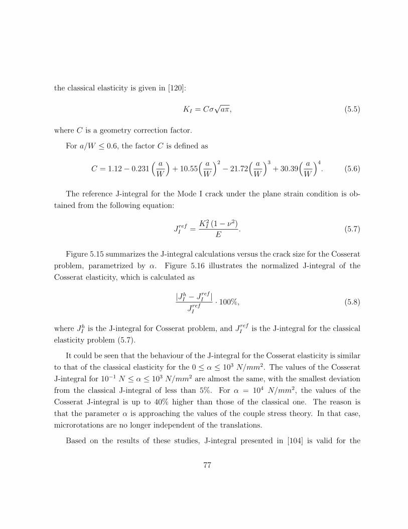
the classical elasticity is given in [120]:

KI = Cσ√aπ, (5.5)

where C is a geometry correction factor.

For a/W ≤ 0.6, the factor C is defined as

C = 1.12− 0.231( aW

)+ 10.55

( aW

)2

− 21.72( aW

)3

+ 30.39( aW

)4

. (5.6)

The reference J-integral for the Mode I crack under the plane strain condition is ob-

tained from the following equation:

JrefI =K2I (1− ν2)

E. (5.7)

Figure 5.15 summarizes the J-integral calculations versus the crack size for the Cosserat

problem, parametrized by α. Figure 5.16 illustrates the normalized J-integral of the

Cosserat elasticity, which is calculated as

|JhI − JrefI |

JrefI

· 100%, (5.8)

where JhI is the J-integral for Cosserat problem, and JrefI is the J-integral for the classical

elasticity problem (5.7).

It could be seen that the behaviour of the J-integral for the Cosserat elasticity is similar

to that of the classical elasticity for the 0 ≤ α ≤ 103 N/mm2. The values of the Cosserat

J-integral for 10−1 N ≤ α ≤ 103 N/mm2 are almost the same, with the smallest deviation

from the classical J-integral of less than 5%. For α = 104 N/mm2, the values of the

Cosserat J-integral is up to 40% higher than those of the classical one. The reason is

that the parameter α is approaching the values of the couple stress theory. In that case,

microrotations are no longer independent of the translations.

Based on the results of these studies, J-integral presented in [104] is valid for the

77

0.1 0.15 0.2 0.25 0.3 0.35 0.4 0.45 0.50

0.2

0.4

0.6

0.8

1

1.2

a/W

J I

ClassicalCosserat alpha=1

Cosserat alpha=102

Cosserat alpha=103

Cosserat alpha=104

Figure 5.15: The J-integral versus the crack length.

calculations of the energy release rate in a Cosserat medium. In addition, the higher

values of J-integral are obtained for the problems with the microrotations involved.

78

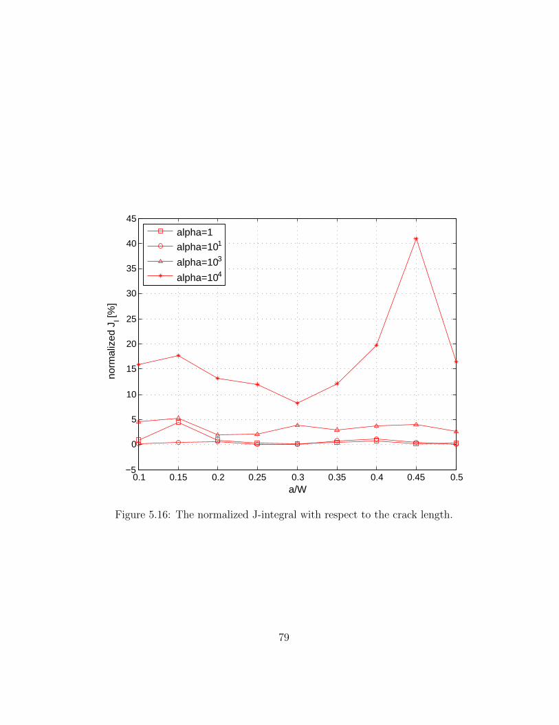
0.1 0.15 0.2 0.25 0.3 0.35 0.4 0.45 0.5−5

0

5

10

15

20

25

30

35

40

45

a/W

norm

aliz

ed J

I [%]

alpha=1

alpha=101

alpha=103

alpha=104

Figure 5.16: The normalized J-integral with respect to the crack length.

79

Chapter 6

Conclusions and Recommendations

This chapter summarizes the main conclusions of the conducted research and makes rec-

ommendations for the future development of fracture modelling in a Cosserat medium.

6.1 Concluding remarks

Several objectives of the present research on crack opening simulation in Cosserat materials

were identified at the beginning of the thesis. The main results and accomplishments of

the research, addressing these objectives, are listed below:

• The primary goal of the research was to develop a robust and efficient method to

simulate cracks in a Cosserat medium. The governing and discrete equations of the

XFEM/Cosserat model were derived and presented in Chapter 4. The model was

verified through the series of patch and convergence tests.

• The convergence study for the Finite Element Method and eXtended Finite Element

Method were presented in Chapter 5. The optimal convergence rates for the XFEM

solution of the Mode I and II edge crack problems were obtained. In addition,

several cases depending on the tip enrichment zone (topological and geometrical)

80

were investigated to get the optimal way to enrich the tip area for the further crack

simulation.

• The calculation of J-integral was verified, allowing for reliance on the developed

numerical technique. Particularly, under a wide range of input parameters, such

as number of elements, the radius of the contour and the number of segments on

the contour, the J-integral calculation exhibits consistent behaviour and predicts the

same exact result.

• The J-integral for the Cosserat elastic medium was compared to the J-integral for the

classical elastic medium, considering the example of the edge crack problem under

tension. It was found that the values of the J-integral of the Cosserat medium were up

to 5% higher than those of the classical elastic medium when the micropolar material

parameter α < 104 N/mm2 was employed. For α ≥ 104 N/mm2, the difference

between the Cosserat and classical J-integral was up to 40% for the same problem.

As mentioned above, parameter α governs the coupling level between translations

and rotations with α = 0 corresponding to the classical elastic problem and α→∞corresponding to the couple stress problem.

6.2 Recommendations for the future development

The proposed XFEM model of an edge crack in a Cosserat medium can be extended in

the several aspects described below.

First, further development of the proposed numerical XFEM/Cosserat model should

address the improvement of the accuracy of the solution. It would be advisable to com-

pare the convergence rates of the method considering various enrichment functions. The

enrichment of the microrotation field is of special interest due to the lack of information

about it in the literature.

Second, the presented model has the simple geometry of a straight line, and only the

opening of the crack is considered; however, real cracks have more complicated geometry.

81

The growth of the curved cracks, multiple and branching cracks in Cosserat media could

be modelled.

Third, the initial XFEM/Cosserat crack model could be extended to the cohesive crack

model. The presented model considers the fracture process zone to be small compared to

the relevant dimensions of the specimen. This assumption neglects detailed description

of what is happening in the fracture process zone. However, in reality, a small plastic

zone will be formed around the crack tip. The cohesive crack model is able to transfer

stress from one crack surface to another and describes the progressive fracture zone in full.

The cohesive cracks in a Cosserat medium have not been studied or modelled in scientific

community.

Considering the possible practical applications, the presented research may be a depar-

ture point to develop an accurate and realistic method for modelling fracture in geome-

chanics. In particular, these are problems of hydraulic fracture in materials such as shale

rocks. The interest in development of the continuous model for the discontinuous rock

masses is that, for the practical applications, a homogenized continuum model describes a

large-scale response of the medium. Moreover, classical continuum theories cannot account

for the elementary bending due to inter-block slip and may considerably overestimate the

deformation [121]. For example, the discontinuous structure of shale rocks may be con-

sidered as the equivalent homogenized continuum using the Cosserat theory. This method

takes into account the physical behaviour of material with a complex microstructure; it

also considers the bending effect between the particles of material during the deformation

by incorporating the intrinsic length scale into the governing equations of the system. The

XFEM/Cosserat model along with the J-integral evaluation technique could be used to

model full fracture process in the shale rock formations.

82

APPENDICES

83

Appendix A

Matrix definitions

The submatrices from the system (4.40) are

K11 =

∫Ω

B>DuBdΩ, (A.1)

K12 =

∫Ω

B>DuTNφdΩ, (A.2)

K13 =

∫Ω

B>DuBdΩ, (A.3)

K14 =

∫Ω

B>DuTNφdΩ, (A.4)

K15 =

∫Ω

B>DuBdΩ, (A.5)

K16 =

∫Ω

B>DuTNφdΩ, (A.6)

84

K21 = −∫Ω

Nφ>T>DuBdΩ, (A.7)

K22 =

∫Ω

(Bφ>DφBφ −Nφ>T>DuTNφ)dΩ, (A.8)

K23 = −∫Ω

Nφ>T>DuBdΩ, (A.9)

K24 =

∫Ω

(Bφ>DφBφ −Nφ>T>DuTN

φ)dΩ, (A.10)

K25 = −∫Ω

Nφ>T>DuBdΩ, (A.11)

K26 =

∫Ω

(Bφ>DφBφ −Nφ>T>DuTNφ)dΩ, (A.12)

K31 =

∫Ω

B>DuBdΩ, (A.13)

K32 =

∫Ω

B>DuTNφdΩ, (A.14)

K33 =

∫Ω

B>DuBdΩ, (A.15)

K34 =

∫Ω

B>DuTN

φdΩ, (A.16)

K35 =

∫Ω

B>DuBdΩ, (A.17)

K36 =

∫Ω

B>DuTNφdΩ, (A.18)

85

K41 = −∫Ω

Nφ>

T>DuBdΩ, (A.19)

K42 =

∫Ω

(Bφ>

DφBφ −Nφ>

T>DuTNφ)dΩ, (A.20)

K43 = −∫Ω

Nφ>

T>DuBdΩ, (A.21)

K44 =

∫Ω

(Bφ>

DφBφ −N

φ>T>DuTN

φ)dΩ, (A.22)

K45 = −∫Ω

Nφ>

T>DuBdΩ, (A.23)

K46 =

∫Ω

(Bφ>

DφBφ −Nφ>

T>DutNφ)dΩ, (A.24)

K51 =

∫Ω

B>DuBdΩ, (A.25)

K52 =

∫Ω

B>DuTNφdΩ, (A.26)

K53 =

∫Ω

B>DuBdΩ, (A.27)

K54 =

∫Ω

B>DuTNφdΩ, (A.28)

K55 =

∫Ω

B>DuBdΩ, (A.29)

K56 =

∫Ω

B>DuTNφdΩ, (A.30)

86

K61 = −∫Ω

Nφ>T>DuBdΩ, (A.31)

K62 =

∫Ω

(Bφ>DφBφ − Nφ>T>DuTNφ)dΩ, (A.32)

K63 = −∫Ω

Nφ>TDuBdΩ, (A.33)

K64 =

∫Ω

(Bφ>DφBφ − Nφ>T>DuTN

φ)dΩ, (A.34)

K65 = −∫Ω

Nφ>T>DuBdΩ, (A.35)

K66 =

∫Ω

(Bφ>DφBφ − Nφ>T>DuTNφ)dΩ, (A.36)

f1 =

∫Γt

N>tdΓ +

∫Ω

N>bσdΩ, (A.37)

f2 =

∫ΓM

Nφ>MdΓ +

∫Ω

Nφ>bmdΩ, (A.38)

f3 =

∫Γt

N>tdΓ +

∫Ω

N>bσdΩ, (A.39)

f4 =

∫ΓM

Nφ>

MdΓ +

∫Ω

Nφ>

bmdΩ, (A.40)

f5 =

∫Γt

N>tdΓ +

∫Ω

N>bσdΩ, (A.41)

f6 =

∫ΓM

Nφ>MdΓ +

∫Ω

Nφ>bmdΩ, (A.42)

where

87

T =

0

0

−1

1

, (A.43)

BI =

NI(x),x 0

0 NI(x),y

0 NI(x),x

NI(x),y 0

, ∀I ∈ SH ,

BφI =

[NI(x),x

NI(x),y

], ∀I ∈ SH ,

BJ =

NJ(x),x(H(f(x))−H(f(xJ))) 0

0 NJ(x),y(H(f(x))−H(f(xJ)))

0 NJ(x),x(H(f(x))−H(f(xJ)))

NJ(x),y(H(f(x))−H(f(xJ))) 0

, ∀J ∈ Scr,

Bφ

J =

[NJ(x),x(H(f(x))−H(f(xJ)))

NJ(x),y(H(f(x))−H(f(xJ)))

], ∀J ∈ Scr,

88

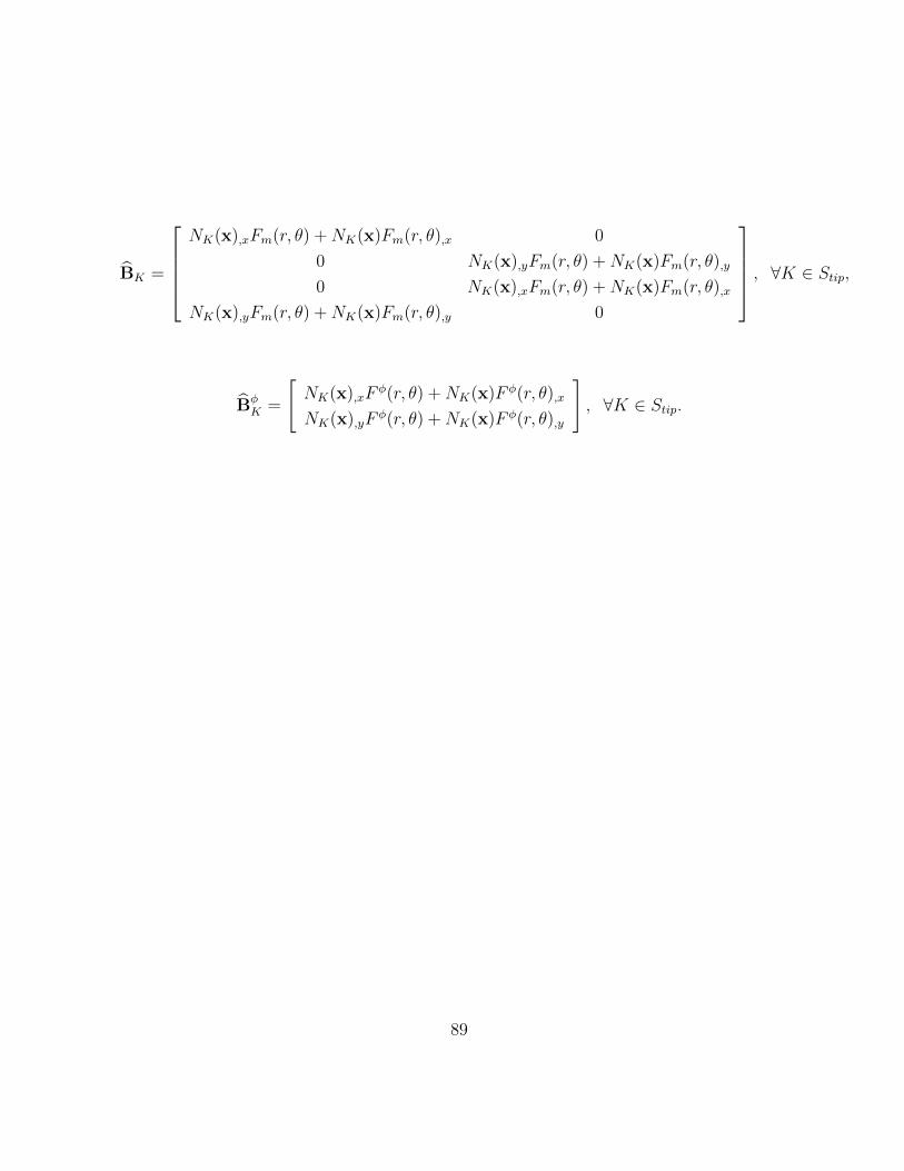
BK =

NK(x),xFm(r, θ) +NK(x)Fm(r, θ),x 0

0 NK(x),yFm(r, θ) +NK(x)Fm(r, θ),y

0 NK(x),xFm(r, θ) +NK(x)Fm(r, θ),x

NK(x),yFm(r, θ) +NK(x)Fm(r, θ),y 0

, ∀K ∈ Stip,

BφK =

[NK(x),xF

φ(r, θ) +NK(x)F φ(r, θ),x

NK(x),yFφ(r, θ) +NK(x)F φ(r, θ),y

], ∀K ∈ Stip.

89

References

[1] A.L. Cauchy. Cours d’analyse de l’Ecole Royale Polytechnique. Imprimerie royale,

1821.

[2] C.L.M.H. Navier. Resume des lecons donnees a l’Ecole royale des ponts et chaussees

sur l’application de la mecanique a l’etablissement des constructions et des machines.

Didot, 1826.

[3] C. Dai, H. Muhlhaus, J. Meek, and M.D. Fama. Modelling of blocky rock masses

using the cosserat method. In International Journal of Rock Mechanics and Mining

Sciences & Geomechanics Abstracts, volume 33, pages 425–432. Pergamon, 1996.

[4] A.R. Khoei and K. Karimi. An enriched-fem model for simulation of localization phe-

nomenon in cosserat continuum theory. Computational Materials Science, 44(2):733–

749, 2008.

[5] A.R. Khoei, S. Yadegari, and S.O.R. Biabanaki. 3d finite element modeling of shear

band localization via the micro-polar cosserat continuum theory. Computational

Materials Science, 49(4):720–733, 2010.

[6] A. Riahi and J.H. Curran. Full 3d finite element cosserat formulation with application

in layered structures. Applied Mathematical Modelling, 33(8):3450–3464, 2009.

[7] M. Gei, M. Rovati, and D. Veber. Effect of internal length scale on optimal topologies

for cosserat continua. In IUTAM Symposium on Topological Design Optimization of

Structures, Machines and Materials, pages 157–166. Springer, 2006.

90

[8] A.C. Eringen. Linear theory of micropolar elasticity. Journal of Mathematics and

Mechanics, 15:909–923, 1966.

[9] E. Cosserat, F. Cosserat, M. Brocato, and K. Chatzis. Theorie des corps deformables.

A. Hermann, 1909.

[10] W. Nowacki. Theory of micropolar elasticity. Springer, 1972.

[11] J.F.C. Yang and R.S. Lakes. Experimental study of micropolar and couple stress

elasticity in compact bone in bending. Journal of biomechanics, 15(2):91–98, 1982.

[12] R.S. Lakes. Size effects and micromechanics of a porous solid. Journal of materials

science, 18(9):2572–2580, 1983.

[13] N.P. Kruyt. Statics and kinematics of discrete cosserat-type granular materials.

International journal of solids and structures, 40(3):511–534, 2003.

[14] I. Munch, P. Neff, and W. Wagner. Transversely isotropic material: nonlinear cosserat

versus classical approach. Continuum Mechanics and Thermodynamics, 23(1):27–34,

2011.

[15] J. Yang and G. Jiang. Experimental study on properties of pervious concrete pave-

ment materials. Cement and Concrete Research, 33(3):381–386, 2003.

[16] J. Fatemi, F. Van Keulen, and PR Onck. Generalized continuum theories: Applica-

tion to stress analysis in bone. Meccanica, 37(4):385–396, 2002.

[17] S.P. Timoshenko and J.N. Goodier. Theory of Elasticity. McGraw-Hill, 1970.

[18] W. Voigt. Theoretische studien fiber die elastizitatsverhiltnisse der kristalle (theoret-

ical studies on the elasticity relationships of crystals). Abh. Gesch. Wissenschaften,

34, 1887.

[19] P. Duhem. Physique et metaphysique. Polleunis, 1893.

[20] R.A. Toupin. Elastic materials with couple-stresses. Archive for Rational Mechanics

and Analysis, 11(1):385–414, 1962.

91

[21] C. Truesdell and R. Toupin. The classical field theories. Springer, 1960.

[22] V.D. Kupradze, T.G. Gelelia, M.O. Basheleıshvili, and T.V. Burchuladze. Three-

dimensional problems in the mathematical theory of elasticity and thermoelasticity:

Classical and micropolar theory. statics, harmonic oscillations, dynamics. fundamen-

tals and solution methods//(russian book). Moscow, Izdatel’stvo Nauka, 1976. 664,

1976.

[23] W. Gunther. Zur statik und kinematik des cosseratschen kontinuums. 1958.

[24] H. Schaefer. Das cosserat kontinuum. ZAMM-Journal of Applied Mathematics and

Mechanics/Zeitschrift fur Angewandte Mathematik und Mechanik, 47(8):485–498,

1967.

[25] H. Schaefer. Analysis der motorfelder im cosserat-kontinuum. ZAMM-Journal of

Applied Mathematics and Mechanics/Zeitschrift fur Angewandte Mathematik und

Mechanik, 47(5):319–328, 1967.

[26] E.L. Aero and E.V. Kuvshinski. Continuum theory of asymmetric elasticity. equilib-

rium of an isotropic body. Solid State Physics, 6(9):2689–2699, 1964.

[27] V.A. Palmov. Fundamental equations of the theory of nonsymmetric elasticity. Prikl.

Math. Mech., 1964.

[28] A.C. Eringen and E.S. Suhubi. Nonlinear theory of simple micro-elastic solids i.

International Journal of Engineering Science, 2(2):189–203, 1964.

[29] R. Lakes. On the torsional properties of single osteons. Journal of biomechanics,

28(11):1409–1409, 1995.

[30] R.S. Lakes. Experimental methods for study of cosserat elastic solids and other

generalized elastic continua. Continuum models for materials with microstructure,

pages 1–25, 1995.

[31] R.S. Lakes and J.F.C. Yang. Micropolar elasticity in bone: rotation modulus κ.

In Proceedings 18th Midwest Mechanics Conference, Iowa City, Developments in

Mechanics, volume 12, pages 239–242, 1983.

92

[32] S. Nakamura and R.S. Lakes. Finite element analysis of stress concentration around

a blunt crack in a cosserat elastic solid. Computer methods in applied mechanics and

engineering, 66(3):257–266, 1988.

[33] P.N. Kaloni and T. Ariman. Stress concentration effects in micropolar elasticity.

Zeitschrift fur Angewandte Mathematik und Physik (ZAMP), 18(1):136–141, 1967.

[34] B.S. Kim. Stress distribution around an elliptic hole in an infinite micropolar elastic

plate. Technical report, DTIC Document, 1973.

[35] R.S. Lakes, S. Nakamura, J.C. Behiri, and W. Bonfield. Fracture mechanics of bone

with short cracks. Journal of biomechanics, 23(10):967–975, 1990.

[36] B. Singh. Continuum characterization of jointed rock masses: Part ithe constitutive

equations. 10(4):311–335, 1973.

[37] B. Singh. Continuum characterization of jointed rock masses: Part iisignificance of

low shear modulus. 10(4):337–349, 1973.

[38] H.B. Muhlhaus. Continuum models for materials with microstructure. Wiley, 1995.

[39] H.B. Muhlhaus and I. Vardoulakis. The thickness of shear bands in granular mate-

rials. Geotechnique, 37(3):271–283, 1987.

[40] C. Dai, H. Muhlhaus, M. Duncan Fama, and J. Meek. Finite element analysis of

cosserat theory for layered rock masses. Computers and Geotechnics, 15(3):145–162,

1993.

[41] H. Yang and K. Wang. Combined identification of constitutive parameters and in-

situ stresses for an elastic cosserat model of an excavation in a layered rock mass.

International Journal of Rock Mechanics and Mining Sciences, 46(3):659–664, 2009.

[42] J. Sulem, I. Vardoulakis, and E. Papamichos. Microstructure and scale effect in gran-

ular rocks. Continuum Models for Materials with Microstructure, H.-B. Muhlhaus,

Ed.(J. Wiley & Sons, Chichester, 1995) pp, pages 200–237, 1995.

93

[43] E. Papamichos. Continua with microstructure: Cosserat theory. European Journal

of Environmental and Civil Engineering, 14(8-9):1011–1029, 2010.

[44] P. Neff. Cosserat theory, 2010.

[45] AC Eringen. Microcontinuum field theories. i. foundations and solids. 1999.

[46] R.S. Lakes. A pathological situation in micropolar elasticity. Journal of applied

mechanics, 52(1):234–235, 1985.

[47] R.D. Gauthier and W.E. Jahsman. A quest for micropolar elastic constants. In

Journal of Applied Mechanics, number 42, pages 369–374, 1975.

[48] J. Ozbolt and Z.P. Bazant. Numerical smeared fracture analysis: Nonlocal microcrack

interaction approach. International Journal for Numerical Methods in Engineering,

39(4):635–662, 1996.

[49] K. Willam, E. Pramono, and S. Sture. Fundamental issues of smeared crack models.

In Proc. SEM-RILEM International Conference on Fracture of Concrete and Rock,

pages 192–207. SEM, Bethel, 1987.

[50] M. Prasad and C.S. Krishnamoorthy. Computational model for discrete crack growth

in plain and reinforced concrete. Computer methods in applied mechanics and engi-

neering, 191(25-26):2699–2725, 2002.

[51] S. Mohammadi. Extended finite element method. Chichester, West Sussex, England:

John Wiley & Sons, 2008.

[52] M. Chaudonneret. On the discontinuity of the stress vector in the boundary in-

tegral equation method for elastic analysis. Recent advances in boundary element

methods.(A 79-38851 16-64) London, Pentech Press, Ltd., pages 185–194, 1978.

[53] S. Potapenko and E. Shmoylova. Solvability of weak solutions to anti-plane cosserat

elasticity by means of boundary integral equations. Mathematics and Mechanics of

Solids, 15(2):209–228, 2010.

94

[54] E. Shmoylova, S. Potapenko, and L. Rothenburg. Boundary element analysis of stress

distribution around a crack in plane micropolar elasticity. International journal of

engineering science, 45(2):199–209, 2007.

[55] A. Portela, M.H. Aliabadi, and D.P. Rooke. The dual boundary element method:

effective implementation for crack problems. International Journal for Numerical

Methods in Engineering, 33(6):1269–1287, 1992.

[56] T. Belytschko and T. Black. Elastic crack growth in finite elements with minimal

remeshing. International Journal for Numerical Methods in Engineering, 45:601–620,

1999.

[57] T. Belytschko and T. Black. Elastic crack growth in finite elements with minimal

remeshing. International Journal for Numerical Methods in Engineering, 45(5):601–

620, 1999.

[58] P.A. Cundall and O.D.L. Strack. A discrete numerical model for granular assemblies.

Geotechnique, 29(1):47–65, 1979.

[59] T. Belytschko, Y. Krongauz, D. Organ, M. Fleming, and P. Krysl. Meshless methods:

an overview and recent developments. Computer methods in applied mechanics and

engineering, 139(1-4):3–47, 1996.

[60] T. Belytschko, N. Moes, S. Usui, and C. Parimi. Arbitrary discontinuities in finite

elements. International Journal for Numerical Methods in Engineering, 50(4):993–

1013, 2001.

[61] T. Belytschko and R. Gracie. On xfem applications to dislocations and interfaces.

International Journal of Plasticity, 23(10-11):1721–1738, 2007.

[62] N. Sukumar, D.L. Chopp, N. Moes, and T. Belytschko. Modeling holes and inclusions

by level sets in the extended finite-element method. Computer Methods in Applied

Mechanics and Engineering, 190:6183–6200, 2001.

95

[63] R. Gracie, G. Ventura, and T. Belytschko. A new fast method for dislocations

based on interior discontinuities. International Journal for Numerical Methods in

Engineering, 69:423–441, 2007.

[64] R. Gracie and T. Belytschko. Concurrently coupled atomistic and xfem models for

dislocations and cracks. International Journal for Numerical Methods in Engineering,

78(3):354–378, 2009.

[65] J. Oswald, R. Gracie, R. Khare, and T. Belytschko. An extended finite element

method for dislocations in complex geometries: thin films and nanotubes. Computer

Methods in Applied Mechanics and Engineering, 198(21-26):1872–1886, 2009.

[66] R. Gracie, J. Oswald, and T. Belytschko. On a new extended finite element method

for dislocations: core enrichments. Journal of the Mechanics and Physics of Solids,

56:200–214, 2008.

[67] Hansbo A. and Hansbo P. A finite element method for the simulation of strong and

weak discontinuities in solid mechanics. Computer Methods in Applied Mechanics

and Engineering, 193:3523–3540, 2004.

[68] T. Belytschko, R. Gracie, and G. Ventura. A review of extended/generalized fi-

nite element methods for material modeling. Modelling and Simulation in Materials

Science and Engineering, 17:043001, 2009.

[69] N. Moes, J. Dolbow, and T. Belytschko. A finite element method for crack growth

without remeshing. International Journal for Numerical Methods in Engineering,

46:131–150, 1999.

[70] J.M. Melenk and I. Babuska. The partition of unity finite element method: Basic

theory and applications. Computer Methods in Applied Mechanics and Engineering,

139:290–314, 1996.

[71] J.E. Dolbow. An extended finite element method with discontinuous enrichment for

applied mechanics. Northwestern University, 1999.

96

[72] J. Dolbow, N. Moes, and T. Belytschko. Discontinuous enrichment in finite elements

with a partition of unity method. Finite Elements in Analysis and Design, 36(3-

4):235–260.

[73] J. Dolbow, N. Moes, and T. Belytschko. Modeling fracture in mindlin–reissner plates

with the extended finite element method. International Journal of Solids and Struc-

tures, 37(48):7161–7183, 2000.

[74] N. Sukumar, N. Moes, B. Moran, and T Belytschko. Extended finite element method

for three-dimensional crack modelling. International Journal for Numerical Methods

in Engineering, 48:1549–1570, 2000.

[75] M. Stolarska, D. L. Chopp, N. Moes, and T. Belytschko. Modelling crack growth by

level sets in the extended finite element method. International Journal for Numerical

Methods in Engineering, 51(8):943–960, 2001.

[76] C. Daux, N. Moes, J. Dolbow, N. Sukumar, and T. Belytschko. Arbitrary branched

and intersecting cracks with the extended finite element method. International Jour-

nal for Numerical Methods in Engineering, 48(12):1741–1760, 2000.

[77] E. Budyn, G. Zi, N. Moes, and T. Belytschko. A method for multiple crack growth

in brittle materials without remeshing. International journal for numerical methods

in engineering, 61(10):1741–1770, 2004.

[78] N. Sukumar and T. Belytschko. Arbitrary branched and intersecting cracks with

the extended finite element method. International Journal for Numerical Methods

in Engineering, 48:1741–1760, 2000.

[79] F.L. Stazi, E. Budyn, J Chessa, and T. Belytschko. An extended finite element

method with higher-order elements for curved cracks. Computational Mechanics,

31:38–48, 2003.

[80] N. Moes and T. Belytschko. Extended finite element method for cohesive crack

growth. Engineering Fracture Mechanics, 69(7):813–833, 2002.

97

[81] J. Dolbow, N. Moes, and T. Belytschko. An extended finite element method for mod-

eling crack growth with frictional contact. Computer Methods in Applied Mechanics

and Engineering, 190(51-52):6825–6846, 2001.

[82] A.R. Khoei and M. Nikbakht. Contact friction modeling with the extended finite

element method (x-fem). Journal of materials processing technology, 177(1):58–62,

2006.

[83] T. Elguedj, A. Gravouil, and A. Combescure. Appropriate extended functions for

x-fem simulation of plastic fracture mechanics. Computer Methods in Applied Me-

chanics and Engineering, 195(7-8):501–515, 2006.

[84] G. Legrain, E. Verron, and N. Moes. Numerical simulation of large strain frac-

ture problems using x-fem. In Constitutve models for rubber-proceedings, volume 4,

page 59. Balkema, 2005.

[85] E. Budyn, T. Hoc, and J. Jonvaux. Fracture strength assessment and aging signs

detection in human cortical bone using an x-fem multiple scale approach. Computa-

tional Mechanics, 42(4):579–591, 2008.

[86] E. Budyn and T. Hoc. Analysis of micro fracture in human haversian cortical bone

under transverse tension using extended physical imaging. International Journal for

Numerical Methods in Engineering, 82(8):940–965, 2010.

[87] X.Y. Liu, Q.Z. Xiao, and B.L. Karihaloo. XFEM for direct evaluation of mixed mode

SIFs in homogeneous and bi-materials. International Journal for Numerical Methods

in Engineering, 59:1103–1118, 2004.

[88] A. Zamani, R. Gracie, and M.R. Eslami. Higher order tip enrichment of extended

finite element method in thermoelasticity. Computational Mechanics, pages 1–16,

2010.

[89] E.E. Gdoutos. Fracture mechanics: an introduction, volume 123. Kluwer Academic

Pub, 2005.

[90] A.A. Griffith. The theory of rupture. 1997.

98

[91] G.P. Cherepanov. The propagation of cracks in a continuous medium. Journal of

Applied Mathematics and Mechanics, 31(3):503–512, 1967.

[92] J.R. Rice. A path independent integral and the approximate analysis of strain con-

centration by notches and cracks. Technical report, DTIC Document, 1967.

[93] T. Anderson. Fracture mechanics: fundamentals and Applications. CRC Press, 1995.

[94] G.R. Irwin. Analysis of stresses and strains near the end of a crack traversing a plate.

J. appl. Mech., 1957.

[95] Z.P. Bazant and J. Planas. Fracture and size effect in concrete and other quasibrittle

materials. CRC, 1998.

[96] H.B. Muhlhaus and E. Pasternak. Path independent integrals for cosserat continua

and application to crack problems. International journal of fracture, 113(4):21–26,

2002.

[97] E. Pasternak, A.V. Dyskin, and H.B. Muhlhaus. Cracks of higher modes in cosserat

continua. International journal of fracture, 140(1):189–199, 2006.

[98] E. Diegele, R. ElsAßer, and C. Tsakmakis. Linear micropolar elastic crack-tip fields

under mixed mode loading conditions. International journal of fracture, 129(4):309–

339, 2004.

[99] G. Exadaktylos, I. Vardoulakis, and E. Aifantis. Cracks in gradient elastic bodies

with surface energy. International Journal of Fracture, 79(2):107–119, 1996.

[100] Y. Huang, L. Zhang, TF Guo, and K.C. Hwang. Mixed mode near-tip fields for cracks

in materials with strain-gradient effects. Journal of the Mechanics and Physics of

Solids, 45(3):439–465, 1997.

[101] L. Zhang, Y. Huang, JY Chen, and KC Hwang. The mode iii full-field solution

in elastic materials with strain gradient effects. International Journal of Fracture,

92(4):325–348, 1998.

99

[102] C. Atkinson and F.G. Leppington. The effect of couple stresses on the tip of a crack.

International Journal of Solids and Structures, 13(11):1103–1122, 1977.

[103] E. Sternberg and R. Muki. The effect of couple-stresses on the stress concentration

around a crack. International Journal of Solids and Structures, 3(1):69–95, 1967.

[104] V.A. Lubarda and X. Markenscoff. On conservation integrals in micropolar elasticity.

Philosophical Magazine, 83(11):1365–1377, 2003.

[105] C. Atkinson and F.G. Leppington. Some calculations of the energy-release rate g

for cracks in micropolar and couple-stress elastic media. International Journal of

Fracture, 10(4):599–602, 1974.

[106] J.D. Eshelby. The elastic energy-momentum tensor. Journal of Elasticity, 5(3):321–

335, 1975.

[107] E. Providas and M.A. Kattis. Finite element method in plane cosserat elasticity. CS,

80(27-30):2059–2069, 2002.

[108] D.U. Yang and F.Y. Huang. Analysis of poissons ratio for a micropolar elastic rectan-

gular plate using the finite element method. Engineering Computations, 18(7):1012–

1030, 2001.

[109] E. Papamichos, I. Vardoulakis, and H.B. Muhlhaus. Buckling of layered elastic

media: A cosserat-continuum approach and its validation. International Journal

for Numerical and Analytical Methods in Geomechanics, 14(7):473–498, 1990.

[110] I. Vardoulakis and E.C. Aifantis. On the role of microstructure in the behavior of

soils: effects of higher order gradients and internal inertia. Mechanics of materials,

18(2):151–158, 1994.

[111] D.P. Adhikary and A.V. Dyskin. A cosserat continuum model for layered materials.

Computers and Geotechnics, 20(1):15–45, 1997.

[112] DP Adhikary and H. Guo. An orthotropic cosserat elasto-plastic model for layered

rocks. Rock mechanics and rock engineering, 35(3):161–170, 2002.

100

[113] A.R. Khoei, M. Anahid, and K. Shahim. An extended arbitrary lagrangian-eulerian

finite element method for large deformation of solid mechanics. Finite Elements in

Analysis and Design, 44(6-7):401–416, 2008.

[114] J. Fish and T. Belytschko. Front Matter. Wiley Online Library, 2007.

[115] J.N. Reddy. An introduction to the finite element method, volume 2. McGraw-Hill

New York, 1993.

[116] T.P. Fries. A corrected xfem approximation without problems in blending elements.

International Journal for Numerical Methods in Engineering, 75(5):503–532, 2008.

[117] G. Ventura, R. Gracie, and T. Belytschko. Fast integration and weight function

blending in the extended finite element method. International Journal for Numerical

Methods in Engineering, 77(1):1–29, 2009.

[118] E. Bechet, H. Minnebo, N. Moes, and B. Burgardt. Improved implementation and

robustness study of the X-FEM for stress analysis around cracks. International

Journal for Numerical Methods in Engineering, 64(8):1033–1056, 2005.

[119] P. Laborde, J. Pommier, Y. Renard, and M. Salaun. High-order extended finite

element method for cracked domains. International Journal for Numerical Methods

in Engineering, 64(3):354–381, 2005.

[120] H. Tada, P.C. Paris, G.R. Irwin, and H. Tada. The stress analysis of cracks handbook,

volume 130. ASME press New York, 2000.

[121] I. Stefanou and J. Sulem. Continuum modeling of discontinuous rock structures.

European Journal of Environmental and Civil Engineering, 14(8-9):1199–1217, 2010.

101